Resource Allocation in Future Green Wireless Networks ...

Resource Allocation in Future Green Wireless Networks:Applications and Challenges

by

Ha Vu TRAN

MANUSCRIPT-BASED THESIS PRESENTED TO ÉCOLE DE

TECHNOLOGIE SUPÉRIEURE IN PARTIAL FULFILLMENT FOR THE

DEGREE OF DOCTOR OF PHILOSOPHY

Ph.D.

MONTREAL, DECEMBER 12, 2019

ÉCOLE DE TECHNOLOGIE SUPÉRIEUREUNIVERSITÉ DU QUÉBEC

Ha Vu Tran, 2019

This Creative Commons license allows readers to download this work and share it with others as long as the

author is credited. The content of this work cannot be modified in any way or used commercially.

BOARD OF EXAMINERS

THIS THESIS HAS BEEN EVALUATED

BY THE FOLLOWING BOARD OF EXAMINERS

M. Georges Kaddoum, Thesis Supervisor

Département de génie électrique, École de Technologie Supérieure

M. Mohamed Faten Zhani, President of the Board of Examiners

Département de génie logiciel et des TI, École de Technologie Supérieure

M. Ghyslain Gagnon, Member of the jury

Département de génie électrique, École de Technologie Supérieure

Mme Gunes Karabulut Kurt, External Independent Examiner

Faculty of Electrical and Electronics Engineering, Istanbul Technical University

THIS THESIS WAS PRESENTED AND DEFENDED

IN THE PRESENCE OF A BOARD OF EXAMINERS AND THE PUBLIC

ON "DECEMBER 4, 2019"

AT ÉCOLE DE TECHNOLOGIE SUPÉRIEURE

FOREWORD

This dissertation is written based on the author’s PhD research outcomes under the supervision

of Professor Georges Kaddoum from September 2015 to August 2019. This work is financially

supported by the Natural Sciences and Engineering Research Council of Canada under Discov-

ery Grant 435243-2013. The main theme of this dissertation focuses on the emerging topic of

resource allocation for green communications for future networks. This dissertation is written

as a monograph based on five published IEEE journal papers and two submitted IEEE journal

papers as the first author.

In this dissertation, the first two chapters present the introduction and the literature review of

green wireless communication networks. Futher, the next seven chapters are wrote based on

my research journal papers. Finally, the conclusion and the recommendation for future work

are given in the last chapter.

ACKNOWLEDGEMENTS

Foremost, I would like to express my most genuine gratefulness to my doctoral supervisor,

Professor Georges Kaddoum, for his support to my PhD study as well as for his patience,

motivation, and encouragement. Actually, I think myself very lucky to have his guidance.

He always shows unrivaled faith in my abilities and gives me the best atmosphere for doing

research. Especially, he knows how to challenge and motivate me to show my best performance

without putting any pressures. I would never have been able to complete my dissertation at its

best without his guidance.

I would like to truly thank all my PhD committee members, Professor Mohamed Faten Zhani,

and Professor Ghyslain Gagnon, for reviewing and giving many constructive comments for

my dissertation. I would also like to thank Professor Gunes Karabulut Kurt for serving as the

external examiner to my PhD defense.

I would like to sincerely thank Dr. Hung Tran and Professor Kien T. Truong for guiding me

at the very first stage of my PhD with helpful advices and making remarkable contributions to

my publications.

My sincere thanks go to my fellow labmates in LACIME. Especially, many thanks to Hamza

Tayeb and Poulmanogo Illy for helping me translate the abstract into French.

I would like to take this oppurtunity to acknowlegde Professor Een-Kee Hong, Dr. Vu Van

Thanh Le, Dr. Hieu Thanh Nguyen, and Dr. Dac-Binh Ha for guiding my research for the past

several years and helping me to develop my background in mathematics, and wireless commu-

nications. I would like to thank my friend, Mr. Duc-Dung Tran, who has been collborating

with me in many research papers.

Last but not least, my sincere thanks go to my parents, younger sister, and all family members

for their endless support and encouragement. Most important than ever, I would never have

been able to finish this long journey without my wife, Dr. Huong Thi Lan Nguyen. Thanks a

million for her understanding when I must be apart from her right away after our marriage due

VIII

to taking up my PhD study in Canada while she was doing her PhD in South Korea. She has

always been supporting, encouraging, cheering me up and stood by me through the good and

bad time. Especially, no words could express my appreciation to her for bringing me “a little

angel” in the next February.

Allocation optimale des ressources dans les futures réseaux sans fil verts : Applicationset défis

Ha Vu TRAN

RÉSUMÉAu cours des récentes dernières années, les réseaux sans fil vertes sont devenues un sujet

émergent vu que l’empreinte carbone des technologies de l’information et de la communica-

tion (TIC) devrait, selon les prévisions, augmenter annuellement de 7,3%, puis dépasser 14%

l’empreinte globale d’ici 2040. De plus, la croissance explosive des TICs, par exemple la cin-

quième génération de réseaux mobiles (5G), prévoit d’atteindre dix fois plus de durée de vie

pour les batteries des appareils et mille fois plus de trafics de données dans les réseaux mobiles

par rapport à la quatrième génération de réseaux mobiles (4G). Les demandes d’augmentation

du débit de données et de la durée de vie des batteries tout en réduisant l’empreinte carbone des

réseaux sans fil de nouvelles générations requièrent une utilisation plus efficace de l’énergie et

bien d’autres ressources. Pour relever ce défi, les concepts de small-cell, energy harvesting,

et les transferts sans fil de données et d’énergie électrique devraient être considérés comme

solutions prometteuses pour reverdir le monde.

Dans cette thèse, les contributions techniques en termes de réduction du coût économique, de

protection des environnements et de garantie de la santé humaine sont fournies. Plus spéci-

fiquement, de nouveaux scénarios de communication sont proposés pour minimiser la con-

sommation d’énergie et ainsi réduire les coûts économiques. De plus, des techniques de re-

cueillement de l’énergie (EH) sont utilisées pour exploiter des ressources vertes disponibles

afin de réduire l’empreinte carbone et ainsi protéger l’environnement. Dans les endroits où

les appareils utilisateurs implémentés ne pourraient pas récupérer l’énergie directement des

ressources naturelles, les stations de base pourraient récupérer et stocker l’énergie verte et

ensuite utiliser cette énergie pour alimenter sans fil les appareils. Cependant, les techniques

de transfert sans fil d’énergie électrique (WPT) devraient être utilisées de manière prudente

pour éviter la pollution électromagnétique et ainsi garantir la santé humaine. Pour atteindre

tous les aspects simultanément, cette thèse propose des schémas prometteurs pour la gestion et

l’allocation optimale des ressources dans les réseaux futurs.

Dans la première partie, le chapitre 2 étudie principalement un schéma de minimisation de la

puissance de transmission pour un réseau 2-tiers hétérogène sur des canaux à évanouissements

selectifs en frequence. De plus, l’interconnexion de réseaux hétérogènes n’est pas capable de

supporter un débit suffisant pour communiquer un échange d’informations entre deux tiers.

Une idée novatrice est introduite dans laquelle la technique “time reversal (TR) beamforming”

est utilisée sur une femtocellule, tandis que la technique “zero-forcing-based beamforming” est

déployée sur une macrocellule. Ainsi, un schéma de minimisation de la puissance de liaison

descendante est proposé et des solutions analytiques optimales sont fournies.

Dans la deuxième partie, les chapitres 3, 4 et 5 se concentrent sur le EH et le transfert sans

fil d’informations et d’énergie électrique en utilisant des signaux fréquence radio (RF). Plus

X

précisément, le chapitre 3 présente un aperçu des progrès récents en matière de radiocommu-

nications vertes et examine les technologies potentielles pour certains thèmes émergents sur

les plateformes EH et WPT. Le chapitre 4 développe une nouvelle architecture intégrée de

récepteurs d’information et d’énergie basée sur l’utilisation directe du courant alternatif pour

le calcul. Il est des montré que l’approche proposée améliore non seulement la capacité de

calcul, mais également l’efficacité énergétique par rapport à l’approche conventionnelle. En

outre, le chapitre 5 propose un nouveau schéma d’allocation de ressources dans les réseaux

de transfert sans fil simultané d’information et d’énergie électrique où trois problèmes cruci-

aux sont traités conjointement: l’amélioration de l’efficacité énergétique, la garantie d’équité

des utilisateurs et l’atténuation de l’effet de réciprocité de canal non idéal. Par conséquent,

de nouvelles méthodes permettant de déduire des solutions optimales et sous-optimales seront

fournies.

Dans la troisième partie, les chapitres 6, 7 et 8 se concentrent sur le transfert simultané d’infor-

mation par ondes lumineuses et énergie électrique (SWIPT) pour des applications intérieures,

en tant que technologie complémentaire au SWIPT RF. Dans cette recherche, le chapitre 6

étudie un réseau à cellules ultra-petites de communication hybride radio fréquence/lumière

visible dans lequel des émetteurs optiques acheminent l’information et l’énergie électrique en

utilisant la lumière visible, tandis qu’un point d’accès radio fréquence travaille comme un sys-

tème complémentaire de transfert d’énergie électrique. Ainsi, un nouveau schéma d’allocation

de ressource exploitant la radio fréquence et la lumière visible pour le transfert d’énergie élec-

trique est conçu. Le chapitre 7 propose l’utilisation du transfert d’énergie par ondes lumineuses

pour permettre la mise en place future et durable des réseaux sans-fil basés sur le Federated

Learning (FL). FL est une nouvelle technique de protection de la confidentialité des données

pour entrainer des modèles d’apprentissage automatique partagés dans une approche distribuée.

Toutefois, l’intégration d’appareils mobiles à contraintes énergétiques pour la construction des

modèles d’apprentissage partagés peut réduire considérablement leur durée de vie. L’approche

proposée peut prendre en charge le réseau sans fil basé sur le FL pour palier le problème de

limitation d’énergie dans les appareils mobiles. Le chapitre 8 présente une nouvelle approche

pour le transfert collaboratif d’énergie électrique par ondes lumineuses et radio fréquence pour

les réseaux de communications sans fil. Les contraintes de puissance de transmission, fixées

par les règles de sécurité, engendrent des défis importants pour améliorer la performance de

transfert d’énergie électrique. Ainsi, l’étude de technologies complémentaires au SWIPT RF

conventionnel est essentielle. Pour faire face à ce problème, ce chapitre propose une nou-

velle technologie collaborative de transfert d’énergie électrique par ondes lumineuses et radio

fréquence pour les réseaux sans fil de prochaine génération.

Mots-clés: communications vertes, réseau hétérogène, recueillement de l’énergie, transfert

sans fil d’énergie électrique, Internet des objets.

Resource Allocation in Future Green Wireless Networks: Applications and Challenges

Ha Vu TRAN

ABSTRACTOver the past few years, green radio communication has been an emerging topic since the foot-

print from the Information and Communication Technologies (ICT) is predicted to increase

7.3% annually and then exceed 14% of the global footprint by 2040. Moreover, the explosive

progress of ICT, e.g., the fifth generation (5G) networks, has resulted in expectations of achiev-

ing 10-fold longer device battery lifetime, and 1000-fold higher global mobile data traffic over

the fourth generation (4G) networks. Therefore, the demands for increasing the data rate and

the lifetime while reducing the footprint in the next-generation wireless networks call for more

efficient utilization of energy and other resources. To overcome this challenge, the concepts

of small-cell, energy harvesting, and wireless information and power transfer networks can be

evaluated as promising solutions for re-greening the world.

In this dissertation, the technical contributions in terms of saving economical cost, protect-

ing the environment, and guaranteeing human health are provided. More specifically, novel

communication scenarios are proposed to minimize energy consumption and hence save eco-

nomic costs. Further, energy harvesting (EH) techniques are applied to exploit available green

resources in order to reduce carbon footprint and then protect the environment. In locations

where implemented user devices might not harvest energy directly from natural resources,

base stations could harvest-and-store green energy and then use such energy to power the de-

vices wirelessly. However, wireless power transfer (WPT) techniques should be used in a wise

manner to avoid electromagnetic pollution and then guarantee human health. To achieve all

these aspects simultaneously, this thesis proposes promising schemes to optimally manage and

allocate resources in future networks.

Given this direction, in the first part, Chapter 2 mainly studies a transmission power mini-

mization scheme for a two-tier heterogeneous network (HetNet) over frequency selective fad-

ing channels. In addition, the HetNet backhaul connection is unable to support a sufficient

throughput for signaling an information exchange between two tiers. A novel idea is intro-

duced in which the time reversal (TR) beamforming technique is used at a femtocell while

zero-forcing-based beamforming is deployed at a macrocell. Thus, a downlink power mini-

mization scheme is proposed, and optimal closed-form solutions are provided.

In the second part, Chapters 3, 4, and 5 concentrate on EH and wireless information and power

transfer (WIPT) using RF signals. More specifically, Chapter 3 presents an overview of the

recent progress in green radio communications and discusses potential technologies for some

emerging topics on the platforms of EH and WPT. Chapter 4 develops a new integrated infor-

mation and energy receiver architecture based on the direct use of alternating current (AC) for

computation. It is shown that the proposed approach enhances not only the computational abil-

ity but also the energy efficiency over the conventional one. Furthermore, Chapter 5 proposes

a novel resource allocation scheme in simultaneous wireless information and power trans-

XII

fer (SWIPT) networks where three crucial issues: power-efficient improvement, user-fairness

guarantee, and non-ideal channel reciprocity effect mitigation, are jointly addressed. Hence,

novel methods to derive optimal and suboptimal solutions are provided.

In the third part, Chapters 6, 7, and 8 focus on simultaneous lightwave information and power

transfer (SLIPT) for indoor applications, as a complementary technology to RF SWIPT. In

this research, Chapter 6 investigates a hybrid RF/visible light communication (VLC) ultra-

small cell network where optical transmitters deliver information and power using the visible

light, whereas an RF access point works as a complementary power transfer system. Thus, a

novel resource allocation scheme exploiting RF and visible light for power transfer is devised.

Chapter 7 proposes the use of lightwave power transfer to enable future sustainable Federated

Learning (FL)-based wireless networks. FL is a new data privacy protection technique for

training shared machine learning models in a distributed approach. However, the involvement

of energy-constrained mobile devices in the construction of the shared learning models may

significantly reduce their lifetime. The proposed approach can support the FL-based wireless

network to overcome the issue of limited energy at mobile devices. Chapter 8 introduces a

novel framework for collaborative RF and lightwave power transfer for wireless communica-

tion networks. The constraints on the transmission power set by safety regulations result in

significant challenges to enhance the power transfer performance. Thus, the study of technolo-

gies complementary to conventional RF SWIPT is essential. To cope with this isue, this chapter

proposes a novel collaborative RF and lightwave power transfer technology for next-generation

wireless networks.

Keywords: green communication, heterogeneous networks, energy harvesting, wireless power

transfer, and IoT.

TABLE OF CONTENTS

Page

INTRODUCTION . . . . . . . . . . . . . . . . . . . . . . . . . . . . . . . . . . . . . . . . . . . . . . . . . . . . . . . . . . . . . . . . . . . . . . . . . . . . . . . . 1

CHAPTER 1 LITERATURE REVIEW OF GREEN WIRELESS NETWORKS:

SMALL-CELL, ENERGY HARVESTING, AND WIRELESS

INFORMATION AND POWER TRANSFER . . . . . . . . . . . . . . . . . . . . . . . . . . . . . 11

1.1 Small-Cell Networks . . . . . . . . . . . . . . . . . . . . . . . . . . . . . . . . . . . . . . . . . . . . . . . . . . . . . . . . . . . . . . . . . . . . 11

1.1.1 The Concept of Small-Cell Networks . . . . . . . . . . . . . . . . . . . . . . . . . . . . . . . . . . . . . . . . 11

1.1.2 Recent Approaches to Green Small-Cell Networks . . . . . . . . . . . . . . . . . . . . . . . . . 12

1.1.2.1 Energy-Efficient Small-Cell Networks . . . . . . . . . . . . . . . . . . . . . . . . . . . 12

1.1.2.2 Transmit Power Minimization in Small-Cell Networks . . . . . . . . . 13

1.1.2.3 Self-Organizing Small-Cell Networks . . . . . . . . . . . . . . . . . . . . . . . . . . . 14

1.2 Energy Harvesting . . . . . . . . . . . . . . . . . . . . . . . . . . . . . . . . . . . . . . . . . . . . . . . . . . . . . . . . . . . . . . . . . . . . . . 16

1.2.1 The Concept of Energy Harvesting . . . . . . . . . . . . . . . . . . . . . . . . . . . . . . . . . . . . . . . . . . 16

1.2.2 Ambient Energy Sources . . . . . . . . . . . . . . . . . . . . . . . . . . . . . . . . . . . . . . . . . . . . . . . . . . . . . 17

1.2.2.1 Solar Energy . . . . . . . . . . . . . . . . . . . . . . . . . . . . . . . . . . . . . . . . . . . . . . . . . . . . . . . 17

1.2.2.2 Wind Energy . . . . . . . . . . . . . . . . . . . . . . . . . . . . . . . . . . . . . . . . . . . . . . . . . . . . . . 17

1.2.2.3 Mechanical Energy . . . . . . . . . . . . . . . . . . . . . . . . . . . . . . . . . . . . . . . . . . . . . . . . 18

1.2.2.4 Thermal Energy . . . . . . . . . . . . . . . . . . . . . . . . . . . . . . . . . . . . . . . . . . . . . . . . . . . 18

1.2.2.5 Radio Frequency Energy . . . . . . . . . . . . . . . . . . . . . . . . . . . . . . . . . . . . . . . . . 18

1.2.2.6 Indoor Artificial Light Energy . . . . . . . . . . . . . . . . . . . . . . . . . . . . . . . . . . . . 19

1.2.3 Energy Harvesting Architectures . . . . . . . . . . . . . . . . . . . . . . . . . . . . . . . . . . . . . . . . . . . . . 19

1.2.3.1 Harvest-Use Architecture . . . . . . . . . . . . . . . . . . . . . . . . . . . . . . . . . . . . . . . . . 20

1.2.3.2 Harvest-Store-Use Architecture . . . . . . . . . . . . . . . . . . . . . . . . . . . . . . . . . . 20

1.2.4 Recent Trends for EH Networks . . . . . . . . . . . . . . . . . . . . . . . . . . . . . . . . . . . . . . . . . . . . . 22

1.2.4.1 EH Networks with Hybrid Natural and On-Grid

Energy Sources . . . . . . . . . . . . . . . . . . . . . . . . . . . . . . . . . . . . . . . . . . . . . . . . . . . . 22

1.2.4.2 EH Networks with RF Sources . . . . . . . . . . . . . . . . . . . . . . . . . . . . . . . . . . . 24

1.3 Wireless Information and Power Transfer . . . . . . . . . . . . . . . . . . . . . . . . . . . . . . . . . . . . . . . . . . . . . 25

1.3.1 The Concept of Wireless Information and Power Transfer . . . . . . . . . . . . . . . . . 25

1.3.1.1 Wireless Power Transfer . . . . . . . . . . . . . . . . . . . . . . . . . . . . . . . . . . . . . . . . . . 25

1.3.2 Wireless Information and Power Transfer . . . . . . . . . . . . . . . . . . . . . . . . . . . . . . . . . . . 28

1.3.3 SWIPT Receiver Architectures . . . . . . . . . . . . . . . . . . . . . . . . . . . . . . . . . . . . . . . . . . . . . . . 29

1.3.3.1 Antenna-Switching Receiver Architecture . . . . . . . . . . . . . . . . . . . . . . . 29

1.3.3.2 Time-Switching Receiver Architecture . . . . . . . . . . . . . . . . . . . . . . . . . . 30

1.3.3.3 Power-switching Receiver Architecture . . . . . . . . . . . . . . . . . . . . . . . . . 31

1.3.3.4 Integrated Receiver Architecture . . . . . . . . . . . . . . . . . . . . . . . . . . . . . . . . . 31

1.3.3.5 Ideal Receiver Architecture . . . . . . . . . . . . . . . . . . . . . . . . . . . . . . . . . . . . . . . 32

1.3.3.6 Comparison between Receiver Designs . . . . . . . . . . . . . . . . . . . . . . . . . . 33

1.3.4 Recent Works in terms of SWIPT Networks . . . . . . . . . . . . . . . . . . . . . . . . . . . . . . . . 34

1.3.4.1 Beamforming Designs for SWIPT Networks . . . . . . . . . . . . . . . . . . . . 34

XIV

1.3.4.2 Cooperative Relay Schemes in SWIPT Networks . . . . . . . . . . . . . . . 36

1.3.4.3 SWIPT Receiver Operation . . . . . . . . . . . . . . . . . . . . . . . . . . . . . . . . . . . . . . . 38

CHAPTER 2 DOWNLINK POWER OPTIMIZATION FOR HETEROGENEOUS

NETWORKS WITH TIME REVERSAL-BASED TRANSMISSION

UNDER BACKHAUL LIMITATION . . . . . . . . . . . . . . . . . . . . . . . . . . . . . . . . . . . . . . . 41

2.1 Introduction . . . . . . . . . . . . . . . . . . . . . . . . . . . . . . . . . . . . . . . . . . . . . . . . . . . . . . . . . . . . . . . . . . . . . . . . . . . . . . 41

2.2 System Model . . . . . . . . . . . . . . . . . . . . . . . . . . . . . . . . . . . . . . . . . . . . . . . . . . . . . . . . . . . . . . . . . . . . . . . . . . . 46

2.3 Beamforming Designs for the MBS and the FBS . . . . . . . . . . . . . . . . . . . . . . . . . . . . . . . . . . . . . 50

2.3.1 Beamformer design following the zero-forcing technique for the

MBS . . . . . . . . . . . . . . . . . . . . . . . . . . . . . . . . . . . . . . . . . . . . . . . . . . . . . . . . . . . . . . . . . . . . . . . . . . . 50

2.3.2 Time Reversal beamforming technique for the FBS . . . . . . . . . . . . . . . . . . . . . . . . 52

2.4 Proposed Power Allocation Approach . . . . . . . . . . . . . . . . . . . . . . . . . . . . . . . . . . . . . . . . . . . . . . . . . 53

2.4.1 Subproblem 1: Power allocation for the FBS . . . . . . . . . . . . . . . . . . . . . . . . . . . . . . . 55

2.4.2 Subproblem 2: Power loading problem for the MBS . . . . . . . . . . . . . . . . . . . . . . . 58

2.5 Worst-case Robust Optimization for TR Femtocell Network . . . . . . . . . . . . . . . . . . . . . . . . . 63

2.5.1 Worst-case lower-bound of signal power component . . . . . . . . . . . . . . . . . . . . . . . 65

2.5.2 Worst-case upper-bound on the ISI power component . . . . . . . . . . . . . . . . . . . . . . 66

2.5.3 Worst-case upper bound on the co-tier interference and objective

function . . . . . . . . . . . . . . . . . . . . . . . . . . . . . . . . . . . . . . . . . . . . . . . . . . . . . . . . . . . . . . . . . . . . . . . . 68

2.6 Numerical Results . . . . . . . . . . . . . . . . . . . . . . . . . . . . . . . . . . . . . . . . . . . . . . . . . . . . . . . . . . . . . . . . . . . . . . . 69

2.6.1 The Proposed Power Allocation Strategy . . . . . . . . . . . . . . . . . . . . . . . . . . . . . . . . . . . . 71

2.6.2 Comparison between TR and zero-forcing techniques . . . . . . . . . . . . . . . . . . . . . . 73

2.6.3 Worst-case Optimization Problem and Performance of Proposed

Upper-bounds . . . . . . . . . . . . . . . . . . . . . . . . . . . . . . . . . . . . . . . . . . . . . . . . . . . . . . . . . . . . . . . . . 74

2.7 Conclusion . . . . . . . . . . . . . . . . . . . . . . . . . . . . . . . . . . . . . . . . . . . . . . . . . . . . . . . . . . . . . . . . . . . . . . . . . . . . . . . 76

CHAPTER 3 RF-WIRELESS POWER TRANSFER: RE-GREENING FUTURE

NETWORKS . . . . . . . . . . . . . . . . . . . . . . . . . . . . . . . . . . . . . . . . . . . . . . . . . . . . . . . . . . . . . . . . . 79

3.1 Introduction . . . . . . . . . . . . . . . . . . . . . . . . . . . . . . . . . . . . . . . . . . . . . . . . . . . . . . . . . . . . . . . . . . . . . . . . . . . . . . 79

3.2 Energy Harvesting and Green RF Wireless Power Transfer . . . . . . . . . . . . . . . . . . . . . . . . . . 80

3.2.1 EH Models . . . . . . . . . . . . . . . . . . . . . . . . . . . . . . . . . . . . . . . . . . . . . . . . . . . . . . . . . . . . . . . . . . . . 80

3.2.2 Green RF Wireless Power Transfer . . . . . . . . . . . . . . . . . . . . . . . . . . . . . . . . . . . . . . . . . . 81

3.3 A Vision of Future Green and EH Networks . . . . . . . . . . . . . . . . . . . . . . . . . . . . . . . . . . . . . . . . . . 83

3.3.1 A predicted model of future green networks with EH . . . . . . . . . . . . . . . . . . . . . . 83

3.3.2 Green radio communications: Main concepts and discussions . . . . . . . . . . . . . 85

3.3.2.1 Full-duplex networks . . . . . . . . . . . . . . . . . . . . . . . . . . . . . . . . . . . . . . . . . . . . . 85

3.3.2.2 Millimeter-wave networks . . . . . . . . . . . . . . . . . . . . . . . . . . . . . . . . . . . . . . . . 85

3.3.2.3 Wireless sensor networks . . . . . . . . . . . . . . . . . . . . . . . . . . . . . . . . . . . . . . . . . 86

3.3.2.4 Cooperative relay networks . . . . . . . . . . . . . . . . . . . . . . . . . . . . . . . . . . . . . . . 87

3.4 Future Research Issues . . . . . . . . . . . . . . . . . . . . . . . . . . . . . . . . . . . . . . . . . . . . . . . . . . . . . . . . . . . . . . . . . . 88

3.4.1 When full-duplex communications meet mm-wave SWIPT

networks? . . . . . . . . . . . . . . . . . . . . . . . . . . . . . . . . . . . . . . . . . . . . . . . . . . . . . . . . . . . . . . . . . . . . . 88

XV

3.4.2 What are potential scenarios for SWIPT and EH HetNets with the

full-duplex technique? . . . . . . . . . . . . . . . . . . . . . . . . . . . . . . . . . . . . . . . . . . . . . . . . . . . . . . . . 89

3.4.3 What are the main concerns of wirelessly powering Internet of

Things networks? . . . . . . . . . . . . . . . . . . . . . . . . . . . . . . . . . . . . . . . . . . . . . . . . . . . . . . . . . . . . . 90

3.5 Concluding Remarks . . . . . . . . . . . . . . . . . . . . . . . . . . . . . . . . . . . . . . . . . . . . . . . . . . . . . . . . . . . . . . . . . . . . 91

CHAPTER 4 ROBUST DESIGN OF AC COMPUTING-ENABLED RECEIVER

ARCHITECTURE FOR SWIPT NETWORKS . . . . . . . . . . . . . . . . . . . . . . . . . . . . 93

4.1 Introduction . . . . . . . . . . . . . . . . . . . . . . . . . . . . . . . . . . . . . . . . . . . . . . . . . . . . . . . . . . . . . . . . . . . . . . . . . . . . . . 93

4.2 System Model . . . . . . . . . . . . . . . . . . . . . . . . . . . . . . . . . . . . . . . . . . . . . . . . . . . . . . . . . . . . . . . . . . . . . . . . . . . 95

4.3 Problem Formulation and Proposed Solution . . . . . . . . . . . . . . . . . . . . . . . . . . . . . . . . . . . . . . . . . . 97

4.3.1 Worst-case Problem Formulation . . . . . . . . . . . . . . . . . . . . . . . . . . . . . . . . . . . . . . . . . . . . 97

4.3.2 Proposed Closed-form Optimal Solution . . . . . . . . . . . . . . . . . . . . . . . . . . . . . . . . . . . . 98

4.3.2.1 Finding w� for a given φ and ρ . . . . . . . . . . . . . . . . . . . . . . . . . . . . . . . . . . 99

4.3.2.2 Finding ρ� and φ� with solved w� . . . . . . . . . . . . . . . . . . . . . . . . . . . . . .100

4.4 Numerical Results . . . . . . . . . . . . . . . . . . . . . . . . . . . . . . . . . . . . . . . . . . . . . . . . . . . . . . . . . . . . . . . . . . . . . .101

4.5 Conclusion . . . . . . . . . . . . . . . . . . . . . . . . . . . . . . . . . . . . . . . . . . . . . . . . . . . . . . . . . . . . . . . . . . . . . . . . . . . . . .103

CHAPTER 5 RESOURCE ALLOCATION IN SWIPT NETWORKS UNDER

A NON-LINEAR ENERGY HARVESTING MODEL: POWER

EFFICIENCY, USER FAIRNESS, AND CHANNEL NON-

RECIPROCITY . . . . . . . . . . . . . . . . . . . . . . . . . . . . . . . . . . . . . . . . . . . . . . . . . . . . . . . . . . . . .105

5.1 Introduction . . . . . . . . . . . . . . . . . . . . . . . . . . . . . . . . . . . . . . . . . . . . . . . . . . . . . . . . . . . . . . . . . . . . . . . . . . . . .105

5.2 System Model . . . . . . . . . . . . . . . . . . . . . . . . . . . . . . . . . . . . . . . . . . . . . . . . . . . . . . . . . . . . . . . . . . . . . . . . . .109

5.2.1 Channel Model of Non-ideal Reciprocity . . . . . . . . . . . . . . . . . . . . . . . . . . . . . . . . . .111

5.2.2 Signal Model . . . . . . . . . . . . . . . . . . . . . . . . . . . . . . . . . . . . . . . . . . . . . . . . . . . . . . . . . . . . . . . . .112

5.2.3 Non-Linear Energy Harvesting Model . . . . . . . . . . . . . . . . . . . . . . . . . . . . . . . . . . . . . .113

5.3 Problem Formulation and Proposed Approach . . . . . . . . . . . . . . . . . . . . . . . . . . . . . . . . . . . . . . .114

5.4 Solutions to the Cross-Layer Multi-Level Optimization Problem . . . . . . . . . . . . . . . . . .118

5.4.1 Solving Upper-Layer Problem OP2 . . . . . . . . . . . . . . . . . . . . . . . . . . . . . . . . . . . . . . . . .119

5.4.2 Solving Second-Level Problem SL1 . . . . . . . . . . . . . . . . . . . . . . . . . . . . . . . . . . . . . . . .123

5.4.3 Analysis of non-linear EH and ID performances on Non-Ideal

Channel Reciprocity . . . . . . . . . . . . . . . . . . . . . . . . . . . . . . . . . . . . . . . . . . . . . . . . . . . . . . . . .125

5.4.4 Optimal and Sub-optimal Solutions for the Problem OP1 . . . . . . . . . . . . . . . . .127


5.5.1 Designing the serving plan at the upper layer . . . . . . . . . . . . . . . . . . . . . . . . . . . . . .133

5.5.2 Performance of the proposed resource allocation scheme . . . . . . . . . . . . . . . . .134

5.5.3 Performance loss due to user mobility, and the suboptimal

solution . . . . . . . . . . . . . . . . . . . . . . . . . . . . . . . . . . . . . . . . . . . . . . . . . . . . . . . . . . . . . . . . . . . . . . .137

5.6 Conclusion . . . . . . . . . . . . . . . . . . . . . . . . . . . . . . . . . . . . . . . . . . . . . . . . . . . . . . . . . . . . . . . . . . . . . . . . . . . . . .140

CHAPTER 6 ULTRA-SMALL CELL NETWORKS WITH COLLABORATIVE

RF AND LIGHTWAVE POWER TRANSFER . . . . . . . . . . . . . . . . . . . . . . . . . . .141

6.1 Introduction . . . . . . . . . . . . . . . . . . . . . . . . . . . . . . . . . . . . . . . . . . . . . . . . . . . . . . . . . . . . . . . . . . . . . . . . . . . . .141

XVI

6.2 System Model . . . . . . . . . . . . . . . . . . . . . . . . . . . . . . . . . . . . . . . . . . . . . . . . . . . . . . . . . . . . . . . . . . . . . . . . . .146

6.2.1 Optical Angle-diversity Transmitters with Color Allocation . . . . . . . . . . . . . .146

6.2.2 VLC Channel Model . . . . . . . . . . . . . . . . . . . . . . . . . . . . . . . . . . . . . . . . . . . . . . . . . . . . . . . . .147

6.2.3 RF Channel Model . . . . . . . . . . . . . . . . . . . . . . . . . . . . . . . . . . . . . . . . . . . . . . . . . . . . . . . . . . .148

6.2.4 Signal Models . . . . . . . . . . . . . . . . . . . . . . . . . . . . . . . . . . . . . . . . . . . . . . . . . . . . . . . . . . . . . . . .149

6.2.4.1 Visible Light Communication . . . . . . . . . . . . . . . . . . . . . . . . . . . . . . . . . . .149

6.2.4.2 VLC Energy Harvesting . . . . . . . . . . . . . . . . . . . . . . . . . . . . . . . . . . . . . . . . .150

6.2.4.3 RF Wireless Power Transfer and Energy Harvesting . . . . . . . . . . .151

6.3 Problem Formulation . . . . . . . . . . . . . . . . . . . . . . . . . . . . . . . . . . . . . . . . . . . . . . . . . . . . . . . . . . . . . . . . . .152

6.4 Proposed Solutions . . . . . . . . . . . . . . . . . . . . . . . . . . . . . . . . . . . . . . . . . . . . . . . . . . . . . . . . . . . . . . . . . . . . .156

6.4.1 Decomposing Problem OP1 without Loss of Optimality . . . . . . . . . . . . . . . . . .156

6.4.2 Solution to Sub-problem SubRF . . . . . . . . . . . . . . . . . . . . . . . . . . . . . . . . . . . . . . . . . . . .158

6.4.3 Optimal Solution to Sub-problems SubVLC . . . . . . . . . . . . . . . . . . . . . . . . . . . . . . .159

6.4.4 Solution to Problem OP2 . . . . . . . . . . . . . . . . . . . . . . . . . . . . . . . . . . . . . . . . . . . . . . . . . . . .162

6.4.5 Suboptimal Solution to SubVLC and Proposed Semi-Decentralized

Approach . . . . . . . . . . . . . . . . . . . . . . . . . . . . . . . . . . . . . . . . . . . . . . . . . . . . . . . . . . . . . . . . . . . . .163


6.6 Conclusion and Future Potential Research . . . . . . . . . . . . . . . . . . . . . . . . . . . . . . . . . . . . . . . . . . . .170

CHAPTER 7 LIGHTWAVE POWER TRANSFER FOR FEDERATED LEARNING-

BASED WIRELESS NETWORKS . . . . . . . . . . . . . . . . . . . . . . . . . . . . . . . . . . . . . . . .173

7.1 Introduction . . . . . . . . . . . . . . . . . . . . . . . . . . . . . . . . . . . . . . . . . . . . . . . . . . . . . . . . . . . . . . . . . . . . . . . . . . . . .173

7.2 System Model . . . . . . . . . . . . . . . . . . . . . . . . . . . . . . . . . . . . . . . . . . . . . . . . . . . . . . . . . . . . . . . . . . . . . . . . . .174

7.2.1 Optical Downlink Wireless Power Transfer . . . . . . . . . . . . . . . . . . . . . . . . . . . . . . . .175

7.2.1.1 Channel Model . . . . . . . . . . . . . . . . . . . . . . . . . . . . . . . . . . . . . . . . . . . . . . . . . . .175

7.2.1.2 Lightwave Energy Harvesting . . . . . . . . . . . . . . . . . . . . . . . . . . . . . . . . . . .176

7.2.2 FL Computation Model . . . . . . . . . . . . . . . . . . . . . . . . . . . . . . . . . . . . . . . . . . . . . . . . . . . . . .177

7.2.3 Radio Frequency Uplink Information Transmission . . . . . . . . . . . . . . . . . . . . . . .177

7.3 Problem Formulation and Proposed Solution . . . . . . . . . . . . . . . . . . . . . . . . . . . . . . . . . . . . . . . . .178

7.3.1 Problem Formulation . . . . . . . . . . . . . . . . . . . . . . . . . . . . . . . . . . . . . . . . . . . . . . . . . . . . . . . .178

7.3.2 Proposed Optimal Solution . . . . . . . . . . . . . . . . . . . . . . . . . . . . . . . . . . . . . . . . . . . . . . . . . .179

7.3.2.1 Optimal Receive Beamformers w�j . . . . . . . . . . . . . . . . . . . . . . . . . . . . . .179

7.3.2.2 Decomposing problem OP1 into subproblems . . . . . . . . . . . . . . . . . .179

7.3.2.3 Optimal Transmission Time T �transj . . . . . . . . . . . . . . . . . . . . . . . . . . . . .181

7.3.2.4 Optimal Power P�1, j . . . . . . . . . . . . . . . . . . . . . . . . . . . . . . . . . . . . . . . . . . . . . . .182


7.5 Conclusion . . . . . . . . . . . . . . . . . . . . . . . . . . . . . . . . . . . . . . . . . . . . . . . . . . . . . . . . . . . . . . . . . . . . . . . . . . . . . .184

CHAPTER 8 COLLABORATIVE RF AND LIGHTWAVE POWER TRANSFER

FOR NEXT-GENERATION WIRELESS NETWORKS . . . . . . . . . . . . . . . . .185

8.1 Introduction . . . . . . . . . . . . . . . . . . . . . . . . . . . . . . . . . . . . . . . . . . . . . . . . . . . . . . . . . . . . . . . . . . . . . . . . . . . . .185

8.2 RF and Lightwave Power Transfer and Related Health Concerns . . . . . . . . . . . . . . . . . . .187

8.2.1 RF Wireless Power Transfer . . . . . . . . . . . . . . . . . . . . . . . . . . . . . . . . . . . . . . . . . . . . . . . . .187

8.2.2 Lightwave Power Transfer: Visible and Infrared Light . . . . . . . . . . . . . . . . . . . .188

XVII

8.3 Enabling Collaborative RF and Lightwave Power Transfer . . . . . . . . . . . . . . . . . . . . . . . . .190

8.3.1 Collaborative RF and Lightwave Power Transfer Architectures . . . . . . . . . .190

8.3.2 Information and Power Transfer Protocols . . . . . . . . . . . . . . . . . . . . . . . . . . . . . . . . .191

8.3.3 Performance of Collaborative RF and Lightwave Power Transfer . . . . . . . .193

8.4 Future Research Opportunities . . . . . . . . . . . . . . . . . . . . . . . . . . . . . . . . . . . . . . . . . . . . . . . . . . . . . . . .195

8.4.1 Indoor Applications . . . . . . . . . . . . . . . . . . . . . . . . . . . . . . . . . . . . . . . . . . . . . . . . . . . . . . . . . .195

8.4.1.1 Secure Wireless Powered Communication Networks . . . . . . . . . .195

8.4.1.2 E-Healthcare . . . . . . . . . . . . . . . . . . . . . . . . . . . . . . . . . . . . . . . . . . . . . . . . . . . . .196

8.4.2 Outdoor Applications . . . . . . . . . . . . . . . . . . . . . . . . . . . . . . . . . . . . . . . . . . . . . . . . . . . . . . . .197

8.4.2.1 Unmanned aerial vehicles . . . . . . . . . . . . . . . . . . . . . . . . . . . . . . . . . . . . . . .197

8.4.2.2 Underwater Communication and Power Transfer . . . . . . . . . . . . . .197

8.5 Conclusion . . . . . . . . . . . . . . . . . . . . . . . . . . . . . . . . . . . . . . . . . . . . . . . . . . . . . . . . . . . . . . . . . . . . . . . . . . . . . .198

CONCLUSION AND RECOMMENDATIONS . . . . . . . . . . . . . . . . . . . . . . . . . . . . . . . . . . . . . . . . . . . . . .199

9.1 Conclusion and Learned Lessons . . . . . . . . . . . . . . . . . . . . . . . . . . . . . . . . . . . . . . . . . . . . . . . . . . . . . .199

9.2 Recommendations: Energy Transfer and Harvesting for 6G networks . . . . . . . . . . . . . .202

9.2.1 Mobile Energy Internet . . . . . . . . . . . . . . . . . . . . . . . . . . . . . . . . . . . . . . . . . . . . . . . . . . . . . .202

9.2.2 Deep Learning for Resource Allocation in Green Wireless

Communications . . . . . . . . . . . . . . . . . . . . . . . . . . . . . . . . . . . . . . . . . . . . . . . . . . . . . . . . . . . . .202

9.2.3 Reinforcement Learning for Self-Organizing Green Wireless

Communications . . . . . . . . . . . . . . . . . . . . . . . . . . . . . . . . . . . . . . . . . . . . . . . . . . . . . . . . . . . . .203

9.2.4 New Green Sources: Invisible Light . . . . . . . . . . . . . . . . . . . . . . . . . . . . . . . . . . . . . . . .203

APPENDIX I APPENDIX OF CHAPTER 2 . . . . . . . . . . . . . . . . . . . . . . . . . . . . . . . . . . . . . . . . . . . . . .205

APPENDIX II APPENDIX OF CHAPTER 4 . . . . . . . . . . . . . . . . . . . . . . . . . . . . . . . . . . . . . . . . . . . . . .211

APPENDIX III APPENDIX OF CHAPTER 5 . . . . . . . . . . . . . . . . . . . . . . . . . . . . . . . . . . . . . . . . . . . . . .213

APPENDIX IV APPENDIX OF CHAPTER 6 . . . . . . . . . . . . . . . . . . . . . . . . . . . . . . . . . . . . . . . . . . . . . .219

BIBLIOGRAPHY . . . . . . . . . . . . . . . . . . . . . . . . . . . . . . . . . . . . . . . . . . . . . . . . . . . . . . . . . . . . . . . . . . . . . . . . . . . . . .223

LIST OF TABLES

Page

Table 1.1 A comparison of three WPT techniques . . . . . . . . . . . . . . . . . . . . . . . . . . . . . . . . . . . . . . . . 27

Table 2.1 The CSI required at MBS. . . . . . . . . . . . . . . . . . . . . . . . . . . . . . . . . . . . . . . . . . . . . . . . . . . . . . . . 56

Table 2.2 ITU indoor office. . . . . . . . . . . . . . . . . . . . . . . . . . . . . . . . . . . . . . . . . . . . . . . . . . . . . . . . . . . . . . . . . 70

Table 2.3 ITU vehicular. . . . . . . . . . . . . . . . . . . . . . . . . . . . . . . . . . . . . . . . . . . . . . . . . . . . . . . . . . . . . . . . . . . . . 70

Table 2.4 ITU outdoor to indoor and pedestrian. . . . . . . . . . . . . . . . . . . . . . . . . . . . . . . . . . . . . . . . . . . 70

Table 2.5 Important parameters . . . . . . . . . . . . . . . . . . . . . . . . . . . . . . . . . . . . . . . . . . . . . . . . . . . . . . . . . . . . 71

Table 5.1 Important parameters . . . . . . . . . . . . . . . . . . . . . . . . . . . . . . . . . . . . . . . . . . . . . . . . . . . . . . . . . . .132

Table 7.1 Important parameters . . . . . . . . . . . . . . . . . . . . . . . . . . . . . . . . . . . . . . . . . . . . . . . . . . . . . . . . . . .182

Table 8.1 RF and lightwave WPT in industry . . . . . . . . . . . . . . . . . . . . . . . . . . . . . . . . . . . . . . . . . . . .188

LIST OF FIGURES

Page

Figure 0.1 ICT footprint as a percentage of total footprint projected through

2040 using both an exponential and linear fits . . . . . . . . . . . . . . . . . . . . . . . . . . . . . . . . . 2

Figure 0.2 Paradigm of the thesis contributions. . . . . . . . . . . . . . . . . . . . . . . . . . . . . . . . . . . . . . . . . . . . 7

Figure 1.1 Harvest-Use Architecture. . . . . . . . . . . . . . . . . . . . . . . . . . . . . . . . . . . . . . . . . . . . . . . . . . . . . . . 20

Figure 1.2 Harvest-Store-Use Architecture . . . . . . . . . . . . . . . . . . . . . . . . . . . . . . . . . . . . . . . . . . . . . . . . 21

Figure 1.3 Wireless Charging Models: (a) inductive coupling, (b) magnetic

resonance coupling, (c) RF wireless energy transfer . . . . . . . . . . . . . . . . . . . . . . . . . . 26

Figure 1.4 SWIPT System . . . . . . . . . . . . . . . . . . . . . . . . . . . . . . . . . . . . . . . . . . . . . . . . . . . . . . . . . . . . . . . . . . 28

Figure 1.5 Antenna-switching receiver . . . . . . . . . . . . . . . . . . . . . . . . . . . . . . . . . . . . . . . . . . . . . . . . . . . . 30

Figure 1.6 Time-switching receiver . . . . . . . . . . . . . . . . . . . . . . . . . . . . . . . . . . . . . . . . . . . . . . . . . . . . . . . . 30

Figure 1.7 Power-switching receiver . . . . . . . . . . . . . . . . . . . . . . . . . . . . . . . . . . . . . . . . . . . . . . . . . . . . . . . 31

Figure 1.8 Integrated receiver . . . . . . . . . . . . . . . . . . . . . . . . . . . . . . . . . . . . . . . . . . . . . . . . . . . . . . . . . . . . . . 32

Figure 1.9 Comparison between receiver designs . . . . . . . . . . . . . . . . . . . . . . . . . . . . . . . . . . . . . . . . . 33

Figure 2.1 A two-tier system model including a macrocell and a femtocell . . . . . . . . . . . . . 46

Figure 2.2 A comparsion between the approaches . . . . . . . . . . . . . . . . . . . . . . . . . . . . . . . . . . . . . . . . 55

Figure 2.3 Performance of power allocation schemes. . . . . . . . . . . . . . . . . . . . . . . . . . . . . . . . . . . . . 71

Figure 2.4 Impact of imperfect{

h10in}N1,N0

j=1,n=1on the performance at a MU . . . . . . . . . . . . . 72

Figure 2.5 A comparison between TR and zero-forcing . . . . . . . . . . . . . . . . . . . . . . . . . . . . . . . . . . 73

Figure 2.6 A comparison between worst-case upper-bounds . . . . . . . . . . . . . . . . . . . . . . . . . . . . . 74

Figure 2.7 Probability distribution per a femtocell user. . . . . . . . . . . . . . . . . . . . . . . . . . . . . . . . . . . 75

Figure 2.8 Transmit power of femtocell with worst-case upper-bounds . . . . . . . . . . . . . . . . . 75

Figure 3.1 Green RF-WPT . . . . . . . . . . . . . . . . . . . . . . . . . . . . . . . . . . . . . . . . . . . . . . . . . . . . . . . . . . . . . . . . . 81

Figure 3.2 A Future Green Network . . . . . . . . . . . . . . . . . . . . . . . . . . . . . . . . . . . . . . . . . . . . . . . . . . . . . . . 83

XXII

Figure 3.3 Mm-wave SWIPT networks with full-duplex communications . . . . . . . . . . . . . . 88

Figure 3.4 SWIPT and EH HetNets with the full-duplex technique . . . . . . . . . . . . . . . . . . . . . . 89

Figure 3.5 RF-WPT Internet of Things networks . . . . . . . . . . . . . . . . . . . . . . . . . . . . . . . . . . . . . . . . . 90

Figure 4.1 Integrated ID and EH Receiver with AC computing . . . . . . . . . . . . . . . . . . . . . . . . . 95

Figure 4.2 Power splitting-based EH receiver architecture with AC computing

. . . . . . . . . . . . . . . . . . . . . . . . . . . . . . . . . . . . . . . . . . . . . . . . . . . . . . . . . . . . . . . . . . . . . . . . . . . . . . . . . . . 97

Figure 4.3 Rate-Energy region, P0 = P−Pcirc = 10 dBm, ψ = 0 . . . . . . . . . . . . . . . . . . . . . . .102

Figure 4.4 Impact of imperfect CSI, P0 = P−Pcirc and ε = 0.2 . . . . . . . . . . . . . . . . . . . . . . . .103

Figure 5.1 An illustration of the SWIPT system including 3 groups of users . . . . . . . . . .110

Figure 5.2 Responsibility for each objective function and each constraint . . . . . . . . . . . . .119

Figure 5.3 The proposed resource allocation scenario . . . . . . . . . . . . . . . . . . . . . . . . . . . . . . . . . .119

Figure 5.4 The trade-off between the two objectives . . . . . . . . . . . . . . . . . . . . . . . . . . . . . . . . . . . . .133

Figure 5.5 Variation of the coverage probability of EH at each user . . . . . . . . . . . . . . . . . . . .134

Figure 5.6 EH performance enhancement (γ = 2 dB) . . . . . . . . . . . . . . . . . . . . . . . . . . . . . . . . . . . .134

(a) EH performance of the overall system. . . . . . . . . . . . . . . . . . . . . . . . . . . . . . . . . . . . . . . .134

(b) EH performance of user 6 in group 3. . . . . . . . . . . . . . . . . . . . . . . . . . . . . . . . . . . . . . . . .134

Figure 5.7 The performance of EH and SINR at user 1 (γ = 2 dB) . . . . . . . . . . . . . . . . . . . . .135

Figure 5.8 A comparison between the proposed scheme and others . . . . . . . . . . . . . . . . . . . .137

Figure 5.9 Performance with the approximations . . . . . . . . . . . . . . . . . . . . . . . . . . . . . . . . . . . . . . . .137

Figure 5.10 Performance loss of the average SINR and the EH . . . . . . . . . . . . . . . . . . . . . . . . . .138

Figure 5.11 Performance loss at near and far users . . . . . . . . . . . . . . . . . . . . . . . . . . . . . . . . . . . . . . . .139

Figure 5.12 A comparison between the optimal and suboptimal solutions (γ =

5). . . . . . . . . . . . . . . . . . . . . . . . . . . . . . . . . . . . . . . . . . . . . . . . . . . . . . . . . . . . . . . . . . . . . . . . . . . . . . . .139

Figure 6.1 An illustration of the network with color allocation . . . . . . . . . . . . . . . . . . . . . . . . .147

Figure 6.2 Visible light communication channel . . . . . . . . . . . . . . . . . . . . . . . . . . . . . . . . . . . . . . . .148

Figure 6.3 The receiver structure of the device with a multi-homing capability . . . . . . .149

XXIII

Figure 6.4 The scenario of solving problems OP1 and OP2 . . . . . . . . . . . . . . . . . . . . . . . . . . . . .154

Figure 6.5 Flowchart of handling OP1. . . . . . . . . . . . . . . . . . . . . . . . . . . . . . . . . . . . . . . . . . . . . . . . . . .162

Figure 6.6 An example of the proposed decentralized scenario . . . . . . . . . . . . . . . . . . . . . . . . .164

Figure 6.7 SNR-EH region at each user . . . . . . . . . . . . . . . . . . . . . . . . . . . . . . . . . . . . . . . . . . . . . . . . . .166

Figure 6.8 Outperformance of the hybrid RF and lightwave power transfer

network . . . . . . . . . . . . . . . . . . . . . . . . . . . . . . . . . . . . . . . . . . . . . . . . . . . . . . . . . . . . . . . . . . . . . . . .167

Figure 6.9 Impact of EH rate allocation, θ RF = 5 and θ = 4 . . . . . . . . . . . . . . . . . . . . . . . . . . .167

Figure 6.10 Transmit power at the RF AP . . . . . . . . . . . . . . . . . . . . . . . . . . . . . . . . . . . . . . . . . . . . . . . . .168

Figure 6.11 Suboptimality of the solution given in Lemma 2 to problem

{SubVLC} . . . . . . . . . . . . . . . . . . . . . . . . . . . . . . . . . . . . . . . . . . . . . . . . . . . . . . . . . . . . . . . . . . . . .169

Figure 6.12 Illuminance in the considered area . . . . . . . . . . . . . . . . . . . . . . . . . . . . . . . . . . . . . . . . . . .170

Figure 7.1 Scenario of lightwave power transfer for FL-based networks . . . . . . . . . . . . . .175

Figure 7.2 Total transmit IRL power versus the uplink rate . . . . . . . . . . . . . . . . . . . . . . . . . . . . .183

Figure 7.3 Transmission time vs. computation time ({θ j}= θ ) . . . . . . . . . . . . . . . . . . . . . . . .184

Figure 8.1 An illustration of the proposed collaborative RF and lightwave

power transfer network . . . . . . . . . . . . . . . . . . . . . . . . . . . . . . . . . . . . . . . . . . . . . . . . . . . . . . .190

Figure 8.2 Proposed transceiver design . . . . . . . . . . . . . . . . . . . . . . . . . . . . . . . . . . . . . . . . . . . . . . . . . . .191

(a) Transmitter architecture . . . . . . . . . . . . . . . . . . . . . . . . . . . . . . . . . . . . . . . . . . . . . . . . . . . . . . .191

(b) Receiver architecture . . . . . . . . . . . . . . . . . . . . . . . . . . . . . . . . . . . . . . . . . . . . . . . . . . . . . . . . . .191

Figure 8.3 Information and power transfer protocols . . . . . . . . . . . . . . . . . . . . . . . . . . . . . . . . . . . .192

Figure 8.4 Heat map of the RF radiation . . . . . . . . . . . . . . . . . . . . . . . . . . . . . . . . . . . . . . . . . . . . . . . . .194

Figure 8.5 Scenarios of collaborative RF and lightwave power transfer . . . . . . . . . . . . . . . .195

(a) Rate-energy region of each approach . . . . . . . . . . . . . . . . . . . . . . . . . . . . . . . . . . . . . . . . .195

(b) Rate-energy region of the proposed protocols . . . . . . . . . . . . . . . . . . . . . . . . . . . . . . . .195

LIST OF ALGORITHMS

Page

Algorithm 2.1 Algorithm to solve umn . . . . . . . . . . . . . . . . . . . . . . . . . . . . . . . . . . . . . . . . . . . . . . . . . . . . . 52

Algorithm 6.1 Algorithm to find B� . . . . . . . . . . . . . . . . . . . . . . . . . . . . . . . . . . . . . . . . . . . . . . . . . . . . . . .161

LIST OF ABREVIATIONS

4G the fourth generation

5G the fifth generation

AC alternating current

ADC analog-to-digital

AN artifical noise

AP access point

AWGN additive white Gaussian noise

BS base station

CEE channel estimation error

CRN cognitive radio network

CIR channel impulse response

CSI channel state information

DC direct current

DRHSCN disaster-resilient heterogeneous small cell network

EH energy harvesting

EIRP equivalent isotropically radiated power

ETSI European Telecommunications Standards Institute

EMF electromagnetic field

FBS femtocell base station

XXVIII

FU femtocell user

GSMA Global Systems for Mobile Communications Association

H-CRAN heterogeneous cloud access radio access networks

HetNet heterogeneous network

HPN high power node

ICF interference channel

ICT information and communication technology

ID information decoding

IoT internet of things

ISI inter-symbol interference

ITU international telecommunication union

MABC multiple acces broadcast

MBS macrocell base station

ML machine learning

MMSE minimum mean square error

mm-wave milimeter wave

MIMO multiple input multiple output

OFDMA orthogonal frequency-division multiple access

OWC optical wireless communication

RF radio frequency

XXIX

RRH remote radio heads

SC super capacitor

SCN small-cell network

SINR signal-to-interference-plus-noise ratio

SISO single input single output

SLIPT simultaneous lightwave information and power transfer

SWIPT simultaneous wireless information and power transfer

TDBC time division broadcast

TDD time division duplex

TDMA time division multiple access

TR time reversal

VLC visible light communication

WPT wireless power transfer

WSN wireless sensor network

ZF zero forcing

LISTE OF SYMBOLS AND UNITS OF MEASUREMENTS

a vector

A matrix

AT the transpose of matrix A

AH the transpose conjugate of matrix A

A† Moore-Penrose generalized inverse of matrix A, A† =(AT A

)−1 AT

tr(A) trace of a matrix A

diag(A) diagonal of matrix A

‖A‖F Frobenius norm

Rm+ the sets of m-dimensional nonnegative real vector

Cm×n the sets of m×n complex matrix

ℜ{.} the real part

ℑ{.} the imaginary part

INTRODUCTION

Motivation, problem statement, and research objective

Future wireless networks, e.g., the fifth generation (5G) networks, are expected to support

multimedia applications to achieve 10-fold longer device battery lifetime and 1000-fold higher

global mobile data traffic, which would surpass 100 ExaBytes (EB) by 2023 Ericsson (2017).

This will escalate the power consumption by which leads to the increasing emission of the

carbon footprint since existing wireless communication systems are mainly supplied by con-

ventional carbon-based power sources.. More specifically, the overall carbon footprint from in-

formation and communication technology (ICT) services, e.g., computer, cell phone, and satel-

lite networks, is predicted to triple in from 2007 to 2020 Fehske, A., Fettweis, G., Malmodin,

J. & Biczok, G. (2011), and to exceed 14% of the global footprint by 2040, as shown in Fig.

0.1. In this context, resource management often faces a dilemma between network perfor-

mance improvement and avoidance of the negative impacts on the natural environment and

human health. Therefore, breakthroughs in information and power transfer to satisfy the wire-

less field are becoming more essential than ever due to the growing demand for more efficient

exploitation of radio frequency (RF) resources. In this context, a challenging topic so-called

next-generation green wireless networks has been emerged in which small-cell, energy harvest-

ing (EH), and wireless information and power transfer (WIPT) concepts have been promoted as

key enabling technologies to reduce the energy consumption and enhance the lifetime of future

networks whereas exploiting green energy sources Agiwal, M., Roy, A. & Saxena, N. (2016);

Buzzi, S., I, C.-L., Klein, T. E., Poor, H. V., Yang, C. & Zappone, A. (2016); Lu, X., Wang, P.,

D., N., Kim, D. I. & Han, Z. (2015b); Wu, Q., Li, G. Y., Chen, W., Ng, D. W. K. & Schober,

R. (2017).

In 5G, the design of new cellular networks tends toward a large-scale deployment of small-

cells, which can potentially realize significant energy savings Wu et al. (2017). Small-cell

2

Figure 0.1 ICT footprint as a percentage of total footprint

projected through 2040 using both an exponential and linear fits

Taken from Belkhir, L. & Elmeligi, A. (2018)

networks (SCNs), which are low-power base stations (BSs) covering a short-range wireless

access for mobile devices, can be classified into distinct types including femtocell, microcell,

and picocell. It has been shown that the small-cell approach can attain a promising gain in

terms of spectral and energy efficiencies due to low power consumption and good ubiquitous

connectivities Agiwal et al. (2016); Hossain, E., Rasti, M., Tabassum, H. & Abdelnasser, A.

(2014). Nevertheless, due to the network densification, multi-tier SCNs face the problems

associated with the management of available resources to avoid resource collisions Buzzi et al.

(2016). Therefore, the power allocation in the SCNs becomes more challenging compared to

conventional single-tier networks.

Considering the SCNs, to further reduce the power consumption constituting the carbon foot-

print, EH has been considered as a promising solution Lu et al. (2015b); Wu et al. (2017). In

principle, the EH paradigm harnesses green energy from natural sources, e.g., solar and wind,

and converts it into electrical current used to supply wireless networks and prolong the lifetime

of smart user devices. Thus, it decreases the overall footprint and then improves the quality

3

of the surrounding environment. Particularly, EH plays an extremely important role in various

applications, including reducing battery replacement costs of wireless sensors working in toxic

environments Ulukus, S., Yener, A., Erkip, E., Simeone, O., Zorzi, M., Grover, P. & Huang,

K. (2015). Nevertheless, the performance of conventional EH is unstable. In more detail, the

amount of harvested energy from natural resources, such as solar and wind, may vary randomly

over time and depend on the locations and weather conditions which are not controllable, sus-

tainable, and always available. For example, there is insufficient sunlight at night to generate

energy, or it is difficult for indoor devices to harvest solar energy.

This motivated the use of a WIPT paradigm Clerckx, B., Zhang, R., Schober, R., Ng, D. W. K.,

Kim, D. I. & Poor, H. V. (2019) where base stations harvest-and-store green energy from

outdoor and then wirelessly transfer energy to indoor devices using RF signals. Hence, battery-

constrained terminal devices can receive information and energy from RF signals whenever it

is necessary. Even though WIPT is a disruptive approach, the performance of RF wireless

power transfer drastically suffers from path loss Clerckx et al. (2019); Niyato, D., Kim, D. I.,

Maso, M. & Han, Z. (2017). Besides, there exist tight restrictions imposed on the transmitted

power since the intensity of microwave radiation can harm human health. Indeed, wireless

devices must satisfy the equivalent isotropically radiated power (EIRP) requirement ruled by

the Federal Communications Commission WHO (2007). For example, a maximum of 36 dBm

EIRP is limited on the 2.4 GHz band.

The discussed issues regarding SCNs, EH, and WIPT are challenging the research community.

Taking those issues into account, this dissertation aims to find solutions for the critical question

of “how to minimize the power consumption and improve the lifetime of future networks while

exploiting green energy sources and retaining electromagnetic pollution?” Different from the

4G network, future wireless communication systems are expected to be a mixture of various

new system concepts, such as RF wireless power transfer (WPT), Li-Fi, Internet of Things

4

(IoT), etc.. Thus, the existing operational schemes also need to be renovated and/or redesigned

to accommodate the advancements of new transmission technologies as well as network appli-

cations.

Contributions and Outline

The organization of this dissertation, which includes 8 chapters, is structured and detailed as

follows. Chapter 1 presents the comprehensive literature review of SCNs, EH, and WIPT in the

scope of next-generation green wireless networks. In this vein, these technologies and hence

the trends for energy-aware communications are presented. Additionally, the review of related

recent works is given.

Chapter 2 presents the first article studying an application of two different beamforming tech-

niques and propose a novel downlink power minimization scheme for a two-tier heterogeneous

network (HetNet) model. In this context, the time reversal (TR) technique is employed at a

femtocell base station, whereby a zero-forcing-based algorithm is used at a macrocell base

station, and the communication channels are subject to frequency selective fading. Addition-

ally, the HetNet backhaul connection is unable to support a sufficient throughput for signaling

and information exchange between two tiers. Given the considered HetNet model, a downlink

power minimization scheme is proposed and closed-form expressions of the optimal solution

are provided in two cases of perfect and imperfect channel estimation at TR-employed femto-

cell.

Chapter 3 presents the second article discussing potential technologies for the emerging topic

of green radio communication where EH and WPT networks are evaluated as promising ap-

proaches. In this article, an overview of recent trends for future green networks on the plat-

forms of EH and WPT is provided. By rethinking the application of RF-WPT, a new concept,

namely green RF-WTP, is introduced. Accordingly, open challenges and promising combina-

5

tions among current technologies, such as small-cell, millimeter (mm) wave, and Internet of

Things (IoT) networks, are discussed in details to seek solutions for the question of how to

re-green the future networks?

Chapter 4 presents the third article developing a novel integrated information and energy re-

ceiver architecture for SWIPT networks inspired by the direct use of alternating current (AC)

for computation. In this context, the AC computing method, in which wirelessly harvested AC

energy is directly used to supply the computing block of receivers, enhances not only com-

putational ability but also the energy efficiency over the conventional direct current (DC) one.

Further, we aim to manage the trade-off between the information decoding (ID) and energy

harvesting (EH) optimally while taking imperfect channel estimation into account. It results

in a worst-case optimization problem of maximizing the data rate under the constraints of an

EH requirement, the energy needed for supplying the AC computational logic, and a transmit

power budget. Then, we propose a method to derive closed-form optimal solutions.

Chapter 5 presents the fourth article proposing a novel resource allocation scheme in SWIPT

networks where three crucial issues: (i) power efficiency improvement, (ii) user-fairness guar-

antee, and (iii) non-ideal channel reciprocity effect mitigation, are jointly addressed. A re-

source allocation scheme jointly addressing such issues can be potentially devised by using

the multi-objective optimization framework. However, the resulting problem might be com-

plex to solve since the three issues hold different characteristics. Therefore, we propose a

novel method to design the resource allocation scheme. In particular, the principle of our

method relies on mathematically structuralizing the issues into a cross-layer multi-level opti-

mization problem. On this basis, we then devise solving algorithms and closed-form solutions.

Moreover, we propose a closed-form suboptimal solution to instantly adapt the CSI changes in

practice while reducing computational burdens.

6

Chapter 6 presents the fifth article investigating the potential of RF and lightwave power trans-

fer in a hybrid RF/visible light communication (VLC) ultra-small cell network. In the network,

the optical transmitters play the primary role and are responsible for delivering information and

power over the visible light, while the RF AP acts as a complementary power transfer system.

Thus, we propose a novel collaborative RF and lightwave resource allocation scheme for hybrid

RF/VLC ultra-small cell networks. The proposed scheme aims to maximize the communica-

tion quality-of-service provided by the VLC under a constraint of total RF and light energy

harvesting performance, while keeping illumination constant and ensuring health safety. This

scheme leads to the formulation of two optimization problems that correspond to the resource

allocation at the optical transmitters and the RF AP. Both problems are optimally solved by

appropriate algorithms. Moreover, we propose a closed-form suboptimal solution with high

accuracy to tackle the optical transmitters’ resource allocation problem, as well as an efficient

semi-decentralized method.

Chapter 7 presents the sixth article proposing the use of lightwave power transfer to enable new

possibilities for the sustainability of future Federated Learning (FL)-based wireless networks.

FL has been recently presented as a new technique for training shared machine learning models

in a distributed manner while respecting data privacy. However, implementing FL in wireless

networks may significantly reduce the lifetime of energy-constrained mobile devices due to

their involvement in the construction of the shared learning models. To handle this issue, we

propose a novel approach at the physical layer based on the application of lightwave power

transfer in the FL-based wireless network and a scheme design to manage the network’s power

efficiency. Hence, we formulate the corresponding optimization problem and then propose a

method to obtain the optimal solution. Numerical results reveal that: with the infrared light

transmit power of 4 W, a mobile device can process data and achieve the uplink rate of 40 kbps

which is sufficient for doing FL tasks, without using the power from the device battery. Hence,

7

the proposed approach can support the FL-based wireless network to overcome the issue of

limited energy at mobile devices.

Chapter 8 presents the seventh article introducing a novel framework for collaborative RF

and lightwave power transfer for wireless communication networks. Relying solely on RF

resources to cope with the expectations of next-generation wireless networks, such as longer

device lifetimes and higher data rates, may no longer be possible. Thus, the investigation of

technologies complementary to conventional RF SWIPT is of critical importance. In this chap-

ter, we propose a novel collaborative RF and lightwave power transfer technology for future

networks where both the RF and lightwave bands can be entirely exploited. We develop the

corresponding system architecture, and design four corresponding collaborative communica-

tion and power transfer protocols in which the use of RF and lightwave can be combined and

optimized over the time and power domains. Further, we show simulation results, and present

potential future research directions.

For convenience, the big picture of this thesis is shown in Fig. 0.2.

Nex

t-gen

erat

ion

gree

n w

irele

ss n

etw

ork

Small-cell heterogeneous network

Energy Harvesting

Wireless Information and Power Transfer

Chapter 2

Chapter 3

Chapter 5

Chapter 6

Chapter 7

Chapter 8

Chapter 4

1

2

3

1

1 2 3

2 3

2 3

1 2 3

2 3

1 2 3

Figure 0.2 Paradigm of the thesis contributions.

8

Author’s Publications

The outcomes of the author’s PhD research are the articles listed below published and submitted

in IEEE journals.

H-V. Tran, Georges Kaddoum, Panagiotis D. Diamantoulakis, Chadi Abou-Rjeily, and George

K. Karagiannidis (2019), Ultra-small Cell Networks with Collaborative RF and Lightw-

ave Power Transfer, IEEE Transactions on Communications, early access.

H-V. Tran and Georges Kaddoum (2019), Robust Design of AC Computing-enabled Receiver

Architecture for SWIPT Networks, IEEE Wireless Communications Letters, 8(3), 801 -

804.

H-V. Tran, G. Kaddoum, and Kien T. Truong (2018), Resource Allocation in SWIPT Networks

under a Nonlinear Energy Harvesting Model: Power Efficiency, User Fairness, and Cha-

nnel Nonreciprocity, IEEE Transactions on Vehicular Technology, 67(9), 8466 - 8480.

H-V. Tran, and G. Kaddoum (2018), RF-wireless power transfer: Re-greening future networks,

IEEE Potentials Magazine, 37(2), 35 - 41.

H-V. Tran, G. Kaddoum, H. Tran, and E.K. Hong (2017), Downlink optimization for heteroge-

neous networks with time reversal-based transmission under backhaul limitation, IEEEAccess, 5, 755-770.

H-V. Tran, Georges Kaddoum, Hany Elgala, Chadi Abou-Rjeily, and Hemani Kaushal (2019),

Lightwave Power Transfer for Federated Learning-based Wireless Networks, OSA Opt-tics Express, under review.

H-V. Tran, Georges Kaddoum, Panagiotis D. Diamantoulakis, Chadi Abou-Rjeily, and George

K. Karagiannidis (2019), Collaborative RF and Lightwave Power Transfer for Next-Gen-

eration Wireless Networks, IEEE Communications Magazine, under review.

Beside the above articles that contribute to the main contents of this dissertation, other publi-

cations that the author was involved in and which are not included in this dissertation are

9

D-D Tran, H-V. Tran (corresponding author), D-B Ha and G. Kaddoum (2019), Secure Trans-

mit Antenna Selection Protocol for MIMO NOMA Networks over Nakagami-m chann-

els, IEEE Systems Journal, early access.

G. Kaddoum, H-V. Tran, L. Kong, and M. Atallah (2017), Design of simultaneous wireless inf-

ormation and power transfer for short reference DCSK communication system, IEEE T-

ransactions on Communications, 65(1), 431-443.

H-V. Tran, and G. Kaddoum (2018), Green cell-less design for RF wireless power transfer net-

works, IEEE Wireless Communications and Networking Conference (WCNC), Barcelona,

Spain.

H-V. Tran, G. Kaddoum, H. Tran, DD Tran, and DB Ha (2016), Time reversal SWIPT networks

with an active eavesdropper: SER-Energy region analysis, IEEE 84th Vehicular Techno-logy Conference (VTC), Montreal, Canada.

H-V. Tran, Hung Tran, G. Kaddoum, Duc-Dung Tran, and Dac-Binh Ha (2015), Effective sec-

recy-SINR analysis of time reversal-employed systems over correlated multi-path chan-

nel, 11th IEEE International Conference on Wireless and Mobile Computing, Network-ing and Communications (WiMob), pp. 527-532.

DD. Tran, H-V. Tran, DB Ha, and G. Kaddoum (2018), Cooperation in NOMA networks under

limited user-to-user communications: solution and analysis, IEEE Wireless Communica-tions and Networking Conference (WCNC), Barcelona, Spain.

Hung Tran, Quach Xuan Truong, H-V. Tran, Elisabeth Uhlemann (2017), Optimal Energy Ha-

rvesting Time and Power Allocation Policy in CRN Under Security Constraints from E-

avesdroppers, IEEE International Symposium on Personal, Indoor and Mobile Radio C-ommunications (PIMRC), Montreal, Canada.

DD. Tran, H-V. Tran, DB Ha, H. Tran, and G. Kaddoum (2016), Performance analysis of two-

way relaying system with RF-EH and multiple antennas, IEEE 84th Vehicular Technol-ogy Conference (VTC), Montreal, Canada.

CHAPTER 1

LITERATURE REVIEW OF GREEN WIRELESS NETWORKS: SMALL-CELL,ENERGY HARVESTING, AND WIRELESS INFORMATION AND POWER

TRANSFER

1.1 Small-Cell Networks

1.1.1 The Concept of Small-Cell Networks

Contemporarily, the world has witnessed the prompt development of wireless technologies.

This appears with the exponentially increasing demands of heterogeneous wireless commu-

nication services over broadband channels. Thus, cellular networks have been developed to

cope with the rising demand for high achievable throughput, seamless coverage, and reason-

able installation costs. Nevertheless, this trend significantly increases the power consumption

of wireless networks. Indeed, the energy cost and CO2 emissions have been promptly growing

due to the operation of cellular networks. Thus, this results in an emerging demand of energy

saving in future wireless networks.

In 5G networks, the concept of small-cell networks has been considered as a promising solu-

tion to enhance the throughput and to overcome the drawbacks of traditional cellular networks

Hossain et al. (2014); Xu, Z., Yang, C., Li, G., Liu, Y. & Xu, S. (2014), such as the inefficient

usage of spectrum and power, dynamic spectrum access, and indoor coverage. In heteroge-

neous small-cell networks, the macrocell serves a large number of users in a wide area whereas

densely deployed low-power cells, such as femtocells, picocells, and microcells, handle a sub-

stantially smaller number of users. Following this approach, not only the coverage range,

throughput, and reliability but also power efficiency can be improved significantly Hossain

et al. (2014); Liu, Y., Zhang, Y., Yu, R. & Xie, S. (2015); Wu et al. (2017).

12

1.1.2 Recent Approaches to Green Small-Cell Networks

1.1.2.1 Energy-Efficient Small-Cell Networks

With restrictions applied on the maximum transmit power, this trend focuses on optimizing

the resource allocation such that the transmit power is fully exploited to improve the energy

efficiency of networks.

The problem of maximizing energy efficiency for downlink orthogonal frequency-division

multiple access (OFDMA) in a HetNet scenario was addressed in Zhang, Z., Zhang, H., Zhao,

Z., Liu, H., Wen, X. & Jing, W. (2013). In the system model, macrocell and femtocell work on

different spectrums, thus there was no cross-tier interference. To reduce the complexity, power

control and subchannel allocation were separated into two stages. The power control was for-

mulated in terms of a non-cooperative game while the subchannel allocation had a common

energy efficiency problem. On this basis, the authors solved the problems with a distributed

algorithm. Obtained results indicate that the proposed algorithm had a lower complexity than

Round-Robin Scheduling and the conventional noncooperative energy-efficient optimization

algorithm.

In Venturino, L., Zappone, A., Risi, C. & Buzzi, S. (2015), the authors studied the problems

of maximizing the global energy efficiency, the weighted sum of the energy efficiencies and

exponentially-weighted multiplication of the energy efficiencies on each subcarrier for a cellu-

lar OFDMA network. In addition, the transmit power allocated for each subcarrier should not

be larger than the ratio of total transmit power at the base station (BS) to the number of subcar-

riers. Accordingly, the algorithms to solve these problems was provided. Precisely, globally

optimal solutions were given for the asymptotic noise-limited regime. The authors claimed that

a proper reduction of the spectral efficiency might result in substantial energy saving in case of

large values of the maximum transmit power.

A scenario of heterogeneous cloud access radio access networks (H-CRANs) was studied in

Peng, M., Zhang, K., Jiang, J., Wang, J. & Wang, W. (2015). To mitigate interference and

13

enhance the energy efficiency, user association with remote radio heads (RRHs)/high power

node (HPN) and the enhancement of traditional soft fractional frequency reuse (S-FFR) is

considered. On this basis, the optimization problem of energy efficiency was formulated to

address the resource allocation. The authors relaxed the original non-convex problem into a

convex one; then they provided the closed-form solution using the Lagrange dual decompo-

sition method. The paper showed that the H-CRAN system model and the resulting resource

allocation could substantially improve the energy efficiency.

In Jiang, Y., Zou, Y., Guo, H., Tsiftsis, T. A., Bhatnagar, M. R., de Lamare, R. C. & Yao, Y.-D.

(2019), the paper investigated an energy efficiency maximization problem for heterogeneous

small-cell networks where a macro BS and a number of low-power small-cell stations serve a

macro-cell user and small-cell users. The authors proposed a joint transmit power and chan-

nel bandwidth allocation scheme to maximize the energy efficiency of small cells constrained

by transmit power and quality-of-service (QoS). Since the formulated optimization problem

is nonconvex, the authors presented a novel two-tier algorithm to achieve optimal solutions.

They demonstrated that their proposed approach outperforms conventional ones with respect

to energy efficiency maximization.

1.1.2.2 Transmit Power Minimization in Small-Cell Networks

In small-cell networks, minimizing the transmit power leads to a significant reduction of the

overall power consumption at the base stations, hence leading to a power efficient design.

The work in Lakshminarayana, S., Assaad, M. & Debbah, M. (2015) focused on transmit power

minimization under time average QoS constraints in an SCN where multiple users are served

in each cell. On this basis, a stochastic optimization problem was formulated to find optimal

downlink beamformers per each time slot. The authors tackled the problem by using Lyapunov

optimization. They further investigated the impact of delays due to information exchange be-

tween small-cell BSs. Moreover, the authors considered additional constraints of channel state

information (CSI) feedback, which result in a joint CSI feedback and beamforming optimiza-

14

tion scheme. Based on simulation results, they claimed that: in modern wireless applications,

such as multimedia apps, where delay tolerance is adjustable, considering the time average

QoS constraints might result in better power savings than using instantaneous QoS constraints.

In Bonnefoi, R., Moy, C. & Palicot, J. (2018), the authors studied the power control scheme

and the cell discontinuous transmission issue in an SCN. They proposed a policy for energy

consumption minimization at each BS for a multi-small-cell network. The simulation results

showed that the proposed policy outperforms other policies. Additionally, it can provide a 6%

performance gain in energy compared to a policy without power control. Furthermore, this

gain can reach up to 11% when the maximum transmit power at each BS is decreased.

In Liu, Z., Zhang, P., Chan, K. Y., Ma, K. & Li, L. (2019), a two-tier femtocell network, where

the communication environment is time-varying and the CSI is imperfect, was considered. The

authors proposed a power control scheme in which a Fuzzy logic system is used to capture the

instantaneous channel gain and the dynamics of the changing channel. Then, in contrast to pre-

vious existing methods, the proposed scheme does not require the knowledge of channel gain

contribution. On this basis, a transmit power minimization is formulated under constraints of

the transmission rate and a power budget. The authors solved this problem by an iterative fast-

convergent algorithm. Simulation results show that the proposed scheme outperforms existing

methods.

1.1.2.3 Self-Organizing Small-Cell Networks

In cellular networks, the traffic load depends on the location and time. For instance, the traf-

fic load might be higher in office areas compared with residential areas during the daytime,

whereas the converse holds during nighttime. Thus, there always exist cells, that are either

underloaded or overloaded. This motivates network-level management in which multiple BSs

can coordinate with each other.

Specifically, since the BS operation consumes a significant amount of energy, selectively switch-

ing some BSs off according to their traffic load can be a promising approach for saving energy.

15

The coverage area of cells in sleep mode can be served by active neighbor cells. This approach

is known as self-organizing networks introduced in the 3GPP standard (3GPP TS 32.521). In

Americas, G. (2009), the different architecture approaches of self-configuring, self-optimizing,

and self-healing were studied for the first time to save costs and enhance network performance

and flexibility.

Moreover, the work in Jo, H.-S., Mun, C., Moon, J. & Yook, J.-G. (2010) proposed a novel

coverage coordination scheme to deal with any unexpected handover of outdoor users. This

scheme was based on the statistic of the interferences and desired signals of femtocell downlink

transmission. Both the self-optimization and the self-configuration were considered for the

pilot transmit power at a femtocell BS. Regarding self-configuration, the femtocell base station

decides the amount of transmit power relying on the strength of interference from neighbor BSs

to guarantee a nearly constant cell coverage. Further, the femtocell performs self-optimization

to control the transmit power such that the femtocell signals are not leaked to the outdoor area

while satisfying system performance.

The network architecture of disaster-resilient heterogeneous small cell networks (DRHSCNs)

was described for the first time in Zhang, H., Jiang, C., Hu, R. Q. & Qian, Y. (2016). On this

basis, self-optimizing techniques, in terms of capacity, mobility robustness, and coverage op-

timization, were proposed. Additionally, self-configuring methods regarding power, neighbor

cell list, and physical cell ID were studied in DRHSCNs. Thus, according to detailed simula-

tion results, the authors showed that the proposed techniques can improve the performance of

the DRHSCNs significantly.

In Amiri, R., Almasi, M. A., Andrews, J. G. & Mehrpouyan, H. (2019), the authors studied

the application of reinforcement learning to a self-organizing HetNet system model, including

macrocells and denser small cells. A distributed power allocation based on Q-learning was

proposed as a self-organization scheme. Extensive simulations with different learning config-

urations are conducted to illustrate the network performance. It was shown that the proposed

16

method can tackle the transmit power minimization problem in the network, whereas remark-

ably decreasing power usage and therefore the interference.

1.2 Energy Harvesting

1.2.1 The Concept of Energy Harvesting

The aim to exploit available green resources in order to reduce carbon footprint and then protect

environments is a global trend towards re-greening the world. This motivates the utilization of

EH to decrease the footprint due to the wireless network operation. EH is the process of

harnessing energy from surrounding environments or mechanical sources (foot strike, finger

strokes), and then converting the latter into electrical energy. The generated electrical current

is then used to power wireless devices. Furthermore, EH has been recognized as a disruptive

paradigm to extend the lifetime of wireless networks Ng, D. W. K. & Schober, R. (2015);

Ulukus et al. (2015); Wu et al. (2017).

There are many reasons to support the applications of EH. For instance, in specific locations,

such as Northern Canada and Africa, bringing fuels to such locations is a challenge. In general,

each BS consumes on average 30,000 liters of diesel per year. The effort of transporting the

fuel to the site can add a significant cost. As a solution, EH from renewable energy resources,

such as solar and wind, is appealing in order to reduce the expenditure of networks as well as

CO2 emissions. Over the last few years, a project entitled “Green Power for Mobile” has been

started by 25 companies under the Global Systems for Mobile Communications Association

(GSMA) Gre (2014). The goal of this project is to exploit green energy sources in developing

countries. 2.5 billion liters of diesel and 6.8 million tons of carbon emissions are expected

to be cut annually. Although the implementation cost of network systems using renewable

energy resources is expensive. Nevertheless, according to the report by GSMA, this cost can

be compensated after less than three years of operation Gre (2014). This reveals that this

green power technology can be a feasible and attractive solution in both technical and financial

aspects.

17

1.2.2 Ambient Energy Sources

Demands for energy is scaling up day by day and therefore exploiting new and efficient en-

ergy resources is one of the primary trends today. In this subsection, we briefly present the

characteristics of some primary energy sources.

1.2.2.1 Solar Energy

Solar energy can be obtained by converting from sunlight into electricity using photovoltaic or

concentrated solar EH techniques. In more details, the photovoltaic method exploits the photo-

electric effect to transform sunlight into electrical current. On the other hand, the concentrated

solar energy method is to focus light into a sharp beam resulting in a heat source. In fact, solar

power is one of the most popular forms of EH. However, the drawback of this approach is that

the energy is generated only when there exists a sufficient sunlight source. Indeed, the use

of solar energy has been employed in many applications in wireless sensor networks Alippi,

C. & Galperti, C. (2008); Hande, A., Polk, T., Walker, W. & Bhatia, D. (2007) and cellular

networks Ng & Schober (2015); Wu et al. (2017).

1.2.2.2 Wind Energy

Wind power has been considered as an efficient source of green energy over the last decade.

Indeed, it even appears before petroleum economy. Wind power can be harvested by deploying

wind turbine farms. Specifically, up to 800 MW can be achieved by a massive turbine farm,

whereas 3 kW can be attained using small residential turbines. In principle, the wind turbine

generator is responsible for converting mechanical energy into electrical energy. Additionally,

the success of harnessing depends on two critical factors, i.e., wind direction and speed. The

American Wind Energy Association evaluates that the wind turbines can generate electrical

power sufficient for over 15 million homes in the USA. This energy is predicted to exceed the

nation’s electricity requirements by more than ten times Onl.

18

1.2.2.3 Mechanical Energy

Mechanical energy is created according to the vibration effects, the motion of living beings, and

noise. Thus, such energy can be harvested from three primary sources, which are machinery

vibrations, human movements, and flow-induced vibrations. In this concern, piezoelectric ma-

terials are utilized to transform the mechanical energy into electrical current or voltage Ammar,

Y., Buhrig, A., Marzencki, M., Charlot, B., Basrour, S., Matou, K. & Renaudin, M. (2005);

Vijayaraghavan, K. & Rajamani, R. (2007). More specifically, this kind of materials helps

convert the effects of pressure, vibrations, and forces into electricity. Particularly, piezoelec-

tric materials are capable of producing an electrical charge when energy storage is available.

However, the main disadvantage relies on their fragility and the potential leakage of charge.

1.2.2.4 Thermal Energy

In principle, thermal energy harvesting exploits a temperature difference, such as the difference

between the human body and the surrounding environment, to produce an electrical current.

For instance, a device located on the human body can harvest the energy generated from the

body using thermogenerators Mateu, L., Codrea, C., Lucas, N., Pollak, M. & Spies, P. (2006).

In general, the phenomena of converting heat energy into electricity is the thermoelectricity.

Nowadays, thermoelectric devices have been employed in various contexts, such as space and

terrestrial applications. For example, the design of microstructured thermoelectric devices is

investigated to address the concern of telecommunication systems in Bottner, H. & et al. (2004).

1.2.2.5 Radio Frequency Energy

Radio signals belonging to a frequency range from 3 kHz to 300 GHz can be used to carry

energy over the air. Different from the mentioned sources, the characteristics of RF sources

can be listed as follows:

- RF sources are controllable and sustainable,

19

- The energy harvested at a receiver is foreseeable,

- The amount of harvested energy depends on the transmit power, propagation loss, and wave-

length.

Therefore, the RF source is one of the most interesting candidates for future applications. In

fact, it has been widely exploited in many interesting forms, such as wireless sensor networks,

implanted body devices, and cellular networks Le, T., Kaddoum, G. & Shin, O. (2018); Lu, X.,

Niyato, D., Wang, P., Kim, D. I. & Han, Z. (2015a); Lu et al. (2015b); Ng & Schober (2015);

Wu et al. (2017).

1.2.2.6 Indoor Artificial Light Energy

Harvesting indoor artificial light energy is an attractive topic in recent years. It relies on that

fact that indoor light sources, i.e., LED bulbs, provide “free” energy to wireless networks since

no extra power is needed from the lighting system. Nevertheless, the intensity of indoor light

is lower than that of the outdoor light, making the applications of indoor light EH challenging.

In more detail, it is 104 times less than the 1000 W/m2 which is the intensity of 1-sun standard

test conditions. Although the amount of achievable harvested indoor light energy is small,

it is enough to supply wireless sensors, as demonstrated in Mathews, I., King, P. J., Stafford,

F. & Frizzell, R. (2016). Moreover, a transparent solar panel named as Wysips Reflect, recently

developed by Sunpartner Technologies wys (2019), can be integrated into phone screens. It

promises to improve the indoor light EH performance substantially.

1.2.3 Energy Harvesting Architectures

Generally speaking, EH architectures can be classified into two types which are (i) Harvest-

Use: Energy is harvested and then is used instantly, and (ii) Harvest-Store-Use: Energy is

harvested as much as possible and then stored for future use.

20

1.2.3.1 Harvest-Use Architecture

Harvesting System

Devices

Harvest-Use

Figure 1.1 Harvest-Use Architecture

Fig. 1.1 illustrates the Harvest-Use architecture. In this case, the EH system directly supplies

a device. Havest-Use EH systems can be implemented to exploit mechanical energy sources,

i.e. pedaling, walking, etc. For example, piezoelectric materials which are placed in a shoe can

deform to distinct extents when running or even walking. Then, the produced energy can be

used to convey RFID signals with respect to tracking the shoe-wearer Shenck, N. & Paradiso,

J. (2001); Starner, T. (1996).

To guarantee the operation of the devices, the power output of the EH system should be higher

than the minimum working threshold. Otherwise, the devices would be disabled since there

is not enough power supplied. As a consequence, the main drawback is that: the unantici-

pated fluctuations of harvested energy close to the threshold might yield the working devices

to vacillate between ON and OFF states.

1.2.3.2 Harvest-Store-Use Architecture

The Harvest-Store-Use architecture is shown in Fig. 1.2. The model is composed of a harvest-

ing system and a component storing harvested energy. In fact, the energy storage is helpful

when the harvested energy is more than the needed energy for the devices’ usage. Such en-

ergy is stored for later uses when there is a lack of produced energy, or the devices need to

21

increase the working performance. The storage component might include two parts of primary

and secondary storages. In this context, the secondary storage can be seen as a backup one. In

particular, the Harvest-Store-Use system can make non-stable but foreseeable energy sources,

such as solar and wind, more favorable in uses Raghunathan, V., Kansal, A., Hsu, J., Friedman,

J. & Srivastava, M. (2005); Taneja, J., Jeong, J. & Culler, D. (2008).

Harvesting System Devices

Harvest-Store-Use

Primary Storage

Secondary Storage

Figure 1.2 Harvest-Store-Use Architecture

Furthermore, the storage technology and recharge techniques are critical since they can affect

system performance significantly. In EH systems, the rechargeable battery, which can be cre-

ated by several technologies using chemical compositions, is the most suitable choice for the

energy storage. In principle, it can be seen as a storage cell that can be recharged by reversing

internal chemical reactions. Nowadays, there exist some popular rechargeable batteries, such

as Lithium Ion (Li-ion), Nickel Cadmium (NiCd), Nickel Metal, Sealed Lead Acid (SLA),

and Hydride (NiMH). Specifically, NiMH and Li-on, two kinds of batteries, can be evaluated

as great choices for EH systems since they are immune from memory effect-loss on energy

capacity, caused by shallow recharge referring to recharging a partially discharged battery.

22

1.2.4 Recent Trends for EH Networks

1.2.4.1 EH Networks with Hybrid Natural and On-Grid Energy Sources

A hybrid energy source can be defined as a combination of a constant energy source and a har-

vesting energy source such as solar, wind, etc. Therefore, designing power allocation schemes

for wireless systems with hybrid energy sources is challenging.

Considering a peer-to-peer communication where the EH transmitter is equipped with a hybrid

energy supply, power allocation schemes in both online and offline fashions were proposed

in Ahmed, E., Eltawil, A. M. & Sabharwal, A. (2013). The objective of the schemes is to

minimize the contribution of the constant energy source. In this context, the energy harvested

from the natural sources was fully exploited to transmit data packets over defined time slots.

Regarding the power allocation scheme, this work shows that the offline fashion outperforms

the online one.

In Ozel, O., Shahzad, K. & Ulukus, S. (2014), the authors studied the data transmission in

an EH system model where a transmitter has hybrid storage with an inefficient battery and a

super-capacitor (SC). The battery has unlimited capacity, whereas the SC has limited storage.

The transmitter can choose either SC or battery to store the harvested energy. The consumed

energy can be drained from the battery and SC at the same time. Given these settings, the

authors provided solutions for the problems of offline throughput maximization in the cases

of (i) a conventional point-to-point communication and (ii) an additive time-linear processing

cost.

The work in Ng & Schober (2015) investigated the resource allocation problem addressing

renewable energy harvesting, secure information, and power transfer in distributed antenna

systems. The central processor plays the role of a core unit connected with all distributed re-

mote radio heads. In this concern, backhaul connections are supposed to be capacity-limited.

The authors assumed that the central processor is supplied by a constant energy source whereas

the distributed RRHs are integrated with conventional energy harvesters. Particularly, the har-

23

vested energy can be shared between the RRHs and the central processor over a micropower

grid. Hence, the RRHs can transmit information and energy to receivers over RF signals. On

this basis, an optimization problem aiming to minimize the transmit power is formulated under

Quality of Service (QoS) constraints in terms of efficient power transfer and secure communi-

cation. The authors provided an algorithm to solve this problem. Importantly, they concluded

that the proposed system can save much more power than the conventional centralized one.

Considering downlink OFDMA networks with a non-ideal hybrid energy supply, to achieve the

minimal grid energy cost, the utilization of a data buffer at user devices and an energy storage

at a BS was proposed to adapt to the unstable nature of renewable energy sources in Chiang,

P., Guruprasad, R. B. & Dey, S. (2018). Further, a low-complexity online management scheme

relying on Lyapunov optimization is developed. It is able to give an asymptotically optimal

performance bound without the knowledge of the stochastic distribution. The numerical results

showed that the proposed approach can substantially reduce the grid power consumption and

improve the QoS compared to other existing schemes.

To reduce the utilization of on-grid energy in HetNets supplied with hybrid energy sources, the

authors in Fletscher, L. A., Suarez, L. A., Grace, D., Peroni, C. V. & Maestre, J. M. (2019)

improved the energy efficiency over short- and long-timescale by using reactive and proactive

management strategies. While there is no storage infrastructure available in the short-timescale

case, a model predictive controller of the RF source behavior with storage support is considered

in the other case. The proposed strategies were analyzed with the data of solar estimations and

wind measurements from Valle de Aburra, Medellin, Colombia and from the Moscow region,

Russian Federation, respectively. Numerical results show that: for the short-term case, the

on-grid energy consumption can be reduced by up to 34%, which is better than other methods.

Meanwhile, for the long-term case, using the model predictive controller can save up to 22%

regarding the on-grid only macro-BS approach.

24

1.2.4.2 EH Networks with RF Sources

Natural resources might not always be available for terminal devices to harvest energy. For

instance, the locations or weather conditions play a crucial role in deciding how much energy

can be harnessed. On the contrary, the user devices in RF-EH networks benefit from stable

and controllable RF energy sources, e.g., base stations. In the following, some recent works on

RF-EH networks are summarized.

Two relaying protocols were proposed for an RF-EH relay node in Nasir, A. A., Zhou, X.,

Durrani, S. & Kennedy, R. A. (2013). These protocols are based on time-switching and

power-splitting with perfect CSI available at the destination node. Thus, the paper studied

both the delay-limited and non-delay-limited transfers, and provided closed-form expressions

of the outage capacity and the ergodic capacity. Further, the authors devised the optimal time-

switching and power-splitting ratios for the two relaying protocols. On this basis, they claimed

that considering the throughput performance, the relaying protocol based on time-switching

outperforms the one based on power-splitting.

In Ju, H. & Zhang, R. (2014b), an extension of the harvest-then-transmit protocol was pro-

posed to deal with the doubly near-far problem using user cooperation. The authors studied

a two-user time division multiple access (TDMA) RF-EH network. Given this model, during

the allocated time slot, the near user is responsible for using its harvested energy to forward

the information of the distant user before conveying its own data. Thus, the time and power

allocation schemes are optimized to maximize the weighted sum-rate. Using user cooperation,

the authors show that the proposed scheduling scheme improves both the user fairness and

throughput significantly.

The work in Krikidis, I., Sasaki, S., Timotheou, S. & Ding, Z. (2014a) investigated the config-

uration of the antenna array at the relay node over MIMO relay communication channels. A

dynamic antenna switching scheme was proposed to schedule a number of the best channels for

information decoding or EH while allocating the remaining channels for EH or information de-

coding. The closed-form outage probability expression for the proposed scheme was derived.

25

Further, the scheme was investigated in the case of co-channel interference and a zero-forcing

receiver employed at the relay node.

A downlink scheduling scheme for an RF-EH network was studied in Morsi, R., Michalopou-

los, D. S. & Schober, R. (2015). This scheme schedules a user for information reception and

the others for harvesting energy in each time slot. Thus, the authors provided two schemes to

manage the information and energy tradeoff. Specifically, the first scheme works based on the

order of normalized SNR whereas the second one chooses the user according to throughput and

SNR criteria. Both schemes were proven to attain user fairness regarding the EH performance.

The work showed the tradeoff between the average EH performance and ergodic capacity un-

der different the orders of SNR. Further, the closed-form expressions of the average harvested

energy and capacity were derived for fading channels.

Particularly, the very recent work in Salman, E., Stanacevic, M., Das, S. & Djuric, P. M. (2018);

Wan, T., Karimi, Y., Stanacevic, M. & Salman, E. (2017,1) proposed and developed a novel AC

computing methodology for wireless powered-IoT devices. Conventionally, the computational

logic component is supplied by DC, resulting in an AC-to-DC conversion loss. The proposed

approach enables the direct use of AC for computation based on charge-recycling theory. It can

decrease the energy consumption, one of the difficulties in realizing the global expandability

of IoT.

1.3 Wireless Information and Power Transfer

1.3.1 The Concept of Wireless Information and Power Transfer

1.3.1.1 Wireless Power Transfer

Conventional EH methods depend on ambient renewable energy sources, such as solar energy

and wind energy, which are unstable and even unforeseeable in some situations. Thus, har-

vesting energy from intentionally generated electromagnetic (EM) sources is a promising al-

26

ternative approach. This motivates the concept of WPT initiated by Nikola Tesla in the 1910’s.

WPT can be defined as a method to convey the electrical energy from a source to wireless de-

vices without using solid wires or conductors. Fig. 1.3 shows the principle of three main WPT

techniques, namely inductive coupling, magnetic resonance coupling, and RF power transfer.

.

.

. Receiver Transmitter

(a) (b)

(c)

Magnetism

Magnetism

Primary Coil

Secondary Coil

Capacitance Primary Coil

Secondary Coil

RF input DC output

Figure 1.3 Wireless Charging Models: (a) inductive coupling,

(b) magnetic resonance coupling, (c) RF wireless energy transfer

Considering the first two techniques, the inductive coupling technique Covic, G. A. & Boys,

J. T. (2013) relies on the magnetic field induction that carries the energy between a primary

coil and a secondary coil. Next, another technique, so-called the magnetic resonance coupling

Kurs, A., Karalis, A., Moffatt, R., Joannopoulos, J. D., Fisher, P. & Soljacic, M. (2007), uti-

lizes an evanescent-wave coupling to generate and transfer the electrical energy between two

resonators. Each resonator is created by using an additional capacitance on an induction coil.

In fact, both the inductive coupling and the magnetic resonance coupling techniques are used

for the applications with near-field wireless transmissions. Therefore, they might not be suit-

27

able for mobile and remote replenishment/charging over a long range, such as wireless sensor

networks and cellular networks.

Unlike the two above techniques, RF power transfer Visser, H. & Vullers, R. (2013) can be seen

as a solution for far-field transmission. In this context, the RF signals with a frequency range

between 3kHz and 300 GHz are used to carry the energy. On this basis, the RF power transfer

is able to remotely recharge a number of wireless devices working in a wide area. However, the

signal strength degrades according to the propagation loss, such as the transmission distance,

fading effects, etc.

Furthermore, Table I shows a comparison between the three primary WPT techniques. We can

observe that the RF WPT technique outperforms the others on the effective energy transfer dis-

tance. However, the main drawback is that it has low energy efficiency in RF-to-DC conversion

due to the propagation loss.

Table 1.1 A comparison of three WPT techniques

WPT Techniques Propagation Charging Distance Applications

Inductive Coupling Non-radiativeFrom a few millimeters

to a few centimeters

Wireless sensor net-

works, mobile elec-

tronics (e.g, smart

phones and tablets)

Magnetic Resonance

CouplingNon-radiative

From a few centime-

ters to a few meters

Mobile electronics,

home appliances,

cell phone charging,

electric vehicle

charging

RF Power Transfer Radiative

Up to several kilome-

ters. Typically, it de-

pends on the perfor-

mance of RF harvest-

ing receiver, the fading

effects, ect.

Cell phone charging,

cellular networks,

wireless sensors,

implanted body de-

vices, plug-in hybrid

electric vehicle

28

1.3.2 Wireless Information and Power Transfer

Indeed, WPT is a very promising technology and might bring many great conveniences for

future wireless networks. However, it comes with some challenging problems, such as spec-

trum sharing between information transmission and power transfer. The reason for this is that

the power transfer occupies a part of the spectrum used for the information transmission. To

avoid the interference to information transmission, we can use orthogonal frequency channels

to transmit information and energy at the same time. Nevertheless, this solution is inefficient.

To overcome the above problem, SWIPT is designed to save the spectrum by using the same

waveform to convey the information and energy simultaneously. Its principle relies on the fact

that any waveforms for the information signal also carry energy which can be converted to the

electrical power. As a consequence, there exists a trade-off between the quality of decoded

information and the amount of harvested energy.

Energy & Information

BS

.

.

.

ID Receiver

ID-EH Receiver

Information Decoding Zone

Energy Harvesting Zone

EH Receiver

Figure 1.4 SWIPT System

A basic SWIPT network system, as illustrated in Fig. 1.4, consists of one multi-antenna trans-

mitter able to transmit jointly the energy and information signals, one ID receiver, one EH

29

receiver, and one ID-EH receiver which is not only able to decode the information but also

harvest the energy.

As shown in Fig. 1.4, the solid and dashed arrows represent the information and energy flows,

respectively. Further, the solid and the dashed curves divide the network area into EH and ID

zones. The reason for this is that the operating power level of EH is much higher than that of

ID. More specifically, the specific ID and EH receivers work under much distinct power sensi-

tivities, i.e., −10 dBm and−60 dBm for the energy and the information receivers, respectively

Zhang, R. & Ho, C. K. (2013). The devices in the information zone can successfully decode the

information sent by the transmitter, whereas the devices in the EH zone can do both harvesting

and decoding efficiently.

1.3.3 SWIPT Receiver Architectures

In practice, there are two challenging issues when it comes to SWIPT systems. First, the

current circuit designs cannot extract the RF energy from the decoded information signals.

Any energy carried by the received RF signals is lost during the decoding process. Second, the

conventional information receiver is optimal for information reception only, not for EH. This

is due to a big gap that exists between power sensitivities of the ID and the EH receivers. Thus,

the design of the receiver architecture plays a vital role in the achievable performance. In the

following, we present an overview of receiver structures used in SWIPT systems.

1.3.3.1 Antenna-Switching Receiver Architecture

Fig. 1.5 depicts a fundamental model of an antenna-switching receiver architecture. In this

architecture, the energy harvester and the information decoder have their own separated an-

tenna(s). Specifically, the antenna array is divided into two sets, and each set is connected to

either the ID or the EH receivers. The most interesting feature of this architecture relies on its

capability of conducting the EH and the ID processes independently. According to the various

30

CSIs observed at the antennas, the antenna-switching scheme can exploit the channel diversity

and flexibly maximize either the performance of the ID or EH.

EH Receiver

Information Receiver

Figure 1.5 Antenna-switching receiver

1.3.3.2 Time-Switching Receiver Architecture

EH Receiver


Time Switching

T

Figure 1.6 Time-switching receiver

A time-switching receiver architecture composed of an ID receiver, an EH receiver and a time-

switcher is shown in Fig. 1.6. Its structure allows the wireless receiver to switch between the

ID receiver or the EH receiver to obtain RF signals. At the transmitter side, the BS decomposes

the transmission block into two separated time slots, one for conveying the energy and the other

31

for transmitting data. At each time slot, different transmit waveforms can be used to optimize

either the energy or information transmission performances. Furthermore, the receiver can

switch the working mode periodically between the harvesting energy and decoding information

phases. Therefore, various rate-energy trade-offs could be achieved by adjusting the length of

such time slots, i.e., the factor α .

1.3.3.3 Power-switching Receiver Architecture

EH Receiver


Power Switching

P

(1 )P

Figure 1.7 Power-switching receiver

The components of a power splitting receiver are illustrated as in Fig. 1.7. In the power-

splitting architecture, the received RF signals are decomposed into two flows for the ID and

EH receivers with different power levels. In this concern, one stream with power ratio β

(0 ≤ β ≤ 1) is used for EH while the rest, with power ratio (1−β ), is used for ID. However,

the BS cannot optimize the transmitted signals for both ID and the EH performanced at the

same time where different rate-energy trade-offs are achieved by adjusting the value of β .

1.3.3.4 Integrated Receiver Architecture

The work in Zhou, X., Zhang, R. & Ho, C. K. (2013) developed an integrated receiver (IntRx)

architecture as shown in Fig. 1.8. Unlike the time-switching and power-switching receivers

that process the RF signals in the RF band, the IntRx splits the signals after converting them

32

into DC. In this case, the information decoder does not need to install low pass filter which

work as an RF band-to-baseband conversion module, since this operation has been integrated

into the energy receiver. In more details, after passing through the dynamic power splitter, the

baseband signal is sampled and then digitalized using an analog-to-digital converter (ADC).

Thus, the integrated receiver architecture has a reduced form. Note that the dynamic power

splitter can work as a time switcher or power splitter.

EH Receiver


Analog-to-Digital Conversion

Decoder

Diode Low-pass filter Battery

Dynamic Power

Splitting

Figure 1.8 Integrated receiver

1.3.3.5 Ideal Receiver Architecture

Some pioneer works in Fouladgar, A. & Simeone, O. (2012); Grover, P. & Sahai, A. (2010);

Popovski, P., Fouladgar, A. & Simeone, O. (2013); Varshney, L. (2008) considered ideal re-

ceiver architectures to provide the theoretical upper bound of receiver’s performance. In view

of the ideal receiver architecture, they assume that the receiver can extract the RF energy from

the decoded signals. However, this assumption is not feasible in practice. The existing circuit

designs cannot extract RF energy from the decoded information carrier concurrently yet. In

33

other words, the total energy carried by the RF message-bearing signals is lost during the ID

process.

1.3.3.6 Comparison between Receiver Designs

Figure 1.9 Comparison between receiver designs

Taken from Bi, S., Ho, C. & Zhang, R. (2015)

As shown in Fig. 1.9, the authors Bi et al. (2015) gave an example to illustrate the key char-

acteristics of the rate-energy regions. Moreover, they investigated three practical receivers and

one ideal receiver in a point-to-point additive white Gaussian noise (AWGN) channel. One can

see that the rate-energy region of the ideal receiver is rectangular since no design tradeoff is in-

volved in this case. A similar rate-energy region is also observed for IntRx. This is because the

optimal strategy uses an infinitesimally small amount of DC for the ID and the remaining DC

for the EH. The rate-energy region of the time-switching receiver is a straight line connecting

the two optimal operating points for EH and ID, respectively. Compared to the time-switching

receiver, the power-switching receiver has a strictly larger rate-energy region.

Indeed, the optimal EH-ID receiver is still unknown. It is unclear whether the non-trivial rate-

energy region between the ideal and the introduced practical receivers could be achieved or

34

not, which is left for future exploration likely involving different domains, such as physics,

circuits, and information theories.

1.3.4 Recent Works in terms of SWIPT Networks

1.3.4.1 Beamforming Designs for SWIPT Networks

Due to the property of spatial multiplexing, multiple antennas and beamforming techniques

can improve the power transfer efficiency significantly, while guaranteeing the high spectral

efficiency of the information transmission. Indeed, beamforming has been considered as a key

technique for feasible implementations of SWIPT networks.

For the first time, the work in Zhang & Ho (2013) addressed the beamforming optimization for

SWIPT systems. The authors considered a SWIPT MIMO wireless broadcast system, includ-

ing a BS and one or two active users. They assumed that the wireless channel is a quasi-static

fading environment and the BS has perfect channel knowledge. For the scenario of two users,

when a user obtains the information from the transmitter, the other one operates as a harvesting

receiver. The work provided the optimal transmission strategy with the trade-off between the

achieved information and energy. A semi-closed-form expression for the optimal covariance

matrix is derived to satisfy rate-energy requirements. For the case of only one working user, the

user harvests energy and decodes information using the same signal simultaneously. An outer

bound for the achievable rate-energy region is shown for practical designs, such as time switch-

ing and power splitting. It is found that the performance bound cannot be generally achieved

due to the fact that the EH receiver cannot decode the information directly. Furthermore, the

wireless powered communication networks benefit from the interferences which increase the

amount of harvested energy. Therefore, this leads to the issue of handling the compromise

between information, harvested energy and interference.

Due to the distributed nature of wireless environments, the message-bearing signal can be

easily eavesdropped and extracted by eavesdroppers. Therefore, secure transmission in MISO

35

SWIPT systems is an extremely important issue. In Ng, D., Lo, E. & Schober, R. (2014), a mul-

tiuser MISO SWIPT system which consists of a transmitter, multiple legitimate receivers, and

multiple passive eavesdroppers was considered. The legitimate receivers were classified into

two types, namely desired receivers and idle receivers. They are able to decode the information

and harvest the energy from RF signals. Particularly, the authors treated the idle receivers as

potential eavesdroppers due to secrecy issues. In this work, a dual use of both the artificial

noise and the energy signals is proposed to enhance energy transfer efficiency and ensure com-

munication security. In particular, when incomplete CSI of the eavesdroppers is available at the

transmitter, the artificial noise and the energy signals are very useful in scaling down the signal

performance at the eavesdroppers. The design of a resource allocation algorithm considering

both artificial noise and energy signals is formulated as a non-convex optimization problem.

Its objective function is to minimize the total transmit power, whereas the constraints take var-

ious requirements into account. To tackle this problem, the authors replaced a non-convex

probabilistic constraint by a tractable convex deterministic one. The reformulated non-convex

optimization problem is solved by a semidefinite programming-based resource allocation algo-

rithm. Furthermore, a suboptimal scheme with low computational complexity is also provided.

Furthermore, accounting for exploiting the spatial degrees of freedom of the channel, the re-

search in Timotheou, S., Krikidis, I., Karachontzitis, S. & Berberidis, K. (2015) investigated a

new technique for MIMO SWIPT systems. In contrast to the well-known time-switching and

power-switching approaches, their technique does not refer to the antenna elements Krikidis

et al. (2014a); Liu, L., Zhang, R. & Chua, K.-C. (2013). Using singular value decomposition

(SVD), the MIMO communication links can be transformed into eigenchannels that can con-

vey either the information or the energy. Considering the practical assumption of imperfect

CSI, the authors assumed that there exists channel estimation error in the decomposition pro-

cess. This generates interference to the eigenchannels, and hence the interference between the

eigenchannels is also addressed. Accordingly, the authors formulated an optimization problem

minimizing the total transmit power with maximum power per eigenchannel, information, and

energy constraints. The problem can be considered as a mixed-integer nonlinear program. The

36

authors provided the optimal solution as well as very close to optimal solutions with robust

computational performance. An optimal polynomial complexity algorithm is further provided

for the problem with no maximum power per eigenchannel constraint. Particularly, using La-

grange theory, a water filling-like procedure for the optimal power allocation is derived when

the eigenchannel assignment is known. Then, a low polynomial complexity algorithm which

induces a near-optimal solution for a broad range of parameter configurations is presented.

In another work, the authors Lee, H., Lee, S., Lee, K., Kong, H. & Lee, I. (2015) considered

the beamforming optimization for SWIPT in MISO interference channels (IFCs). The system

model consisted of an information transmitter, an information receiver, an energy transmitter,

and an energy receiver. The paper proposed two cooperation categories. The first one con-

sidered a partial cooperation (PCoop) scheme, in which only CSI was available at transmitters

and receivers (except the signal waveform). The second one addressed IFC with full signal

cooperation (SCoop), where both the CSI and the signal waveforms were known by transmit-

ters and receivers, was examined. They constituted the non-convex optimization problems for

IFC-PCoop and IFC-SCoop, respectively, where the information rate was maximized under

minimum required harvested energy constraints to obtain the Pareto boundary. To solve these

problems, the original problem was separated into two subproblems with the introduction of

two new parameters so-called energy splitting and power splitting metrics, for the IFC-PCoop

and the IFCSC, respectively. Accordingly, the closed-form solutions were provided by using

the line search method.

1.3.4.2 Cooperative Relay Schemes in SWIPT Networks

The cooperative relaying technique is one of the best solutions to overcome the attenuation

and fading effects by using the help of intermediate relay stations. By applying cooperative

relaying, the network’s reliability and efficiency can be improved. Therefore, this technique is

highly useful in SWIPT networks where the path loss is one of the most important issues.

37

A SWIPT relay network, in which source-destination (S-D) pairs communicate with each other

with the help of the assigned EH relays, was investigated in Chen, H. H., Li, Y., Jiang, Y., Ma,

Y. & Vucetic, B. (2015). At each relay (R), the received signal was split into two streams

dedicated for either information forwarding or energy harvesting. With the aim of improving

network-wide performance, the authors used the game theory to develop a scheme of dis-

tributed power splitting for the considered system model. In this context, each S-R-D link

was considered as a strategic player who tried to maximize the corresponding individual rate.

Further, the formulated games were studied in terms of Nash equilibriums. After that, the

authors studied the extension of mixed amplify-and-forward and decode-and-forward relays.

To this end, they showed that the proposed algorithm can attain near-optimal solutions for the

network-wide performance.

In Zeng, Y. & Zhang, R. (2016), the authors studied a wireless-powered amplify-and-forward

relay system where a multi-antenna source node transmits information to a single-antenna des-

tination node with the help of a multi-antenna full-duplex relay node. The proposed protocol

can be described as follows. In the first phase, the source node transmits information to the

relay node. In the second phase, at the same time, the relay forwards the amplified information

signal to the destination and receives the energy signal from the source node. The proposed

protocol takes two main advantages: (i) uninterrupted information transmission is guaranteed

since there is no time and power-sharing/switching, and (ii) self-energy recycling is exploited,

i.e., at the relay node, a part of the transmit signal interfering with the receive antennas can be

harvested and re-used. Given the system model and the protocol, the authors devised the opti-

mal power allocation and beamformers for the relay node. The paper showed that the protocol

can achieve a significant throughput enhancement compared to the conventional time-switching

relay protocol.

The authors Ding, Z., Krikidis, I., Sharif, B. & Poor, H. V. (2014) considered a SWIPT cooper-

ative network in which decode-forward relays are randomly located. In the first scenario, one

S-D pair and multiple EH relays were studied. Three different relay configurations were taken

into account. Accordingly, by means of stochastic geometry, the performances regarding diver-

38

sity enhancement and outage probability are depicted. Based on analytical results, the authors

claimed that wisely chosen EH relays can attain the same diversity gain as the self-powered

relays. Nonetheless, the outage probability in the case of EH relays is higher than the one in

the conventional case. In the second scenario, the authors considered the presence of multiple

sources. In particular, such sources compete with each other in order to obtain the help of

the EH relays. This competition is formulated as a coalition formation game. Accordingly, to

address this problem, two game theory-based algorithms were proposed relying on different

payoff functions.

1.3.4.3 SWIPT Receiver Operation

In principle, ID-EH receivers use the same antenna array for both information reception and

EH. Thus, most of the existing works follow the time-switching and power-splitting designs.

Moreover, they have mainly investigated the trade-off in various circumstances to satisfy spe-

cific performance goals. In what follows, some recent works are summarized.

In Liu et al. (2013), a time-switching based policy for a time-varying fading channel was

investigated. First, for the case with unknown CSI at the BS, a time-switching policy was

proposed to leverage the ID and EH performances opportunistically. Second, when the CSI

was available at the BS, the authors jointly designed a transmit power allocation and receiver

policy. The policy coordinates the receiver to harvest energy when channel gain is higher than

a preset threshold and to decode information otherwise. Some complexity-reduced policies

were also provided, one of them works according to co-channel interference. Importantly,

the authors concluded that optimal trade-off between ID and EH performances implies that

allocating the best channels to energy transfer is preferred to information transmission.

The work in Zhou et al. (2013) developed an integrated receiver architecture by generalizing

the time-switching and power-splitting cases. The receiver policy allows the RF signal to be

dynamically split into two streams over time for ID and EH. Further, a special case of the

policy, so-called on-off power-splitting, was proposed. In the off mode, all RF signals are fed

39

to the energy harvester. On the other hand, the receiver works as a power splitter in the on

mode. Based on the analytical and simulation results, the authors concluded that the on-off is

optimal for co-located and integrated receivers when circuit power consumption is taken into

account.

The paper Zhou, X. (2014) investigated how to achieve the maximal ergodic capacity for a

power-splitting receiver by designing a training phase. The authors proposed using a block-

wise transmission scheme including training and transmission phases. On this basis, an op-

timal power-splitting scheme was designed for both phases to maximize the ergodic capacity

whereas satisfying the EH requirements. Further, the authors provided non-adaptive/adaptive

power-splitting schemes in which the splitting factors were fixed/adjusted in all blocks during

the transmission phase. They showed that both schemes can achieve optimal solutions. In

particular, the adaptive scheme outperforms the non-adaptive one with respect to the capacity

where the performance gap is higher when more EH rate is required.

CHAPTER 2

DOWNLINK POWER OPTIMIZATION FOR HETEROGENEOUS NETWORKSWITH TIME REVERSAL-BASED TRANSMISSION UNDER BACKHAUL

LIMITATION

Ha-Vu Tran1, Georges Kaddoum1, Hung Tran2, and Een-Kee Hong3

1 Department of Electrical Engineering, École de Technologie Supérieure,

1100 Notre-Dame west, Montreal, Canada H3C 1K3.2 School of Innovation, Design and Engineering,

Mälardalen University, Västerås, Sweden 721 23.3 School of Electronics and Information, Kyung Hee University,

Yongin, South Korea 449-701.

Paper published in IEEE Access, vol. 5, pp. 755-770, January 2017.

2.1 Introduction

Recently, heterogeneous network (HetNet) has been considered as a promising solution to

enhance the throughput and to overcome the drawbacks of traditional cellular networks Buzzi

et al. (2016); Hossain, E. & Hasan, M. (2015); Zahir, T., Arshad, K., Nakata, A. & Moessner,

K. (2013), such as the inefficient usage of spectrum and dynamic spectrum access. According

to the heterogeneous network (HetNet) concept, the macrocell serves a large number of users in

a wide area while low power cells such as femtocells, picocells and microcells handle a smaller

number of users. Following this approach, not only the coverage range is expanded but also the

throughput and reliability can be improved significantly. More specifically, the works reported

in Andrews, J., Claussen, H., Dohler, M., Rangan, S. & Reed, M. (2012); Buzzi et al. (2016);

Hossain & Hasan (2015); Zahir et al. (2013) have investigated a HetNet model in which an

original cellular network is decomposed into multi-tier networks, and each tier is responsible

for a specific zone. These approaches have expanded the coverage ranges over the dead zones

and hot zones of traditional cellular networks. Therefore, the femtocell is considered as one

of the most cost-efficient provisioning for cellular network services Bennis, M., Giupponi, L.,

Diaz, E., Lalam, M., Maqbool, M., Strinati, E., De Domenico, A. & Latva-aho, M. (2011).

42

Regarding the radio environment, the signal power is often degraded due to path-loss effects

and multipath propagation, and such an issue becomes more severe in the frequency selective

fading. On the other hand, many techniques have been employed to mitigate the adverse effects

of frequency selective channels such as: equalizers, multiple-input multipleoutput (MIMO)

and time reversal (TR) techniques. When applied to wireless receivers, the first two techniques

provide significant enhancement to the received signal-to-noise ratio (SNR). However, from the

implementation point of view, these techniques are high-cost and require complex equipment

which make them less interesting to be used at the subscriber end where limited energy and

processing resources are the major constraints.

However, a special class of beamforming technique, namely the time reversal (TR), which

was mainly used in acoustics and underwater communication systems, has been proposed in

Bouzigues, M.-A., Siaud, I., Helard, M. & Ulmer-Moll, A.-M. (2013); Chen, Y., Wang, B.,

Han, Y., Lai, H.-Q., Safar, Z. & Liu, K. R. (2016b); Kaiser, T. & Zheng, F. (2010); Maaz,

M., Helard, M., Mary, P. & Liu, M. (2015); Pitarokoilis, A., Mohammed, S. & Larsson, E.

(2015); Siaud, I., Ulmer-Moll, A.-M., Bouzigues, M.-A. & Cassiau, N. (2015); Tran-Ha, V.,

Vu, Q.-D. & Hong, E.-K. (2015); Viteri-Mera, C. A., Teixeira, F. L. & Sainath, K. (2015) to

wireless communications, e.g. ultra-wideband, large-scale antenna, and millimeter-wave sys-

tems. This techique provides a promising solution to save the processing cost and to combat

the adverse effects of frequency selective fading channels. Benefiting from the reciprocal prop-

erties of wireless channels, the TR technique principles rely on using the time-reversed form of

a channel impulse response (CIR) to pre-filter the transmitted signal which leads to the power

convergence of this latter in the time and space domains at the receiver side. Specifically, the

CIR at the transmitter side is estimated by virtue of a pilot signal sent from the receiver.

Particularly, some works have addressed the designs of TR beamforming. In Bouzigues et al.

(2013), the authors have provided an analysis of the TR technique for green radio communica-

tions employed to WiFi-certified technologies. The work Viteri-Mera, C. A. & Teixeira, F. L.

(2016) proposes three forms of space-time block diagonalization on the platform of the TR

technique. Further, Yang et.al. Yang, Y.-H., Wang, B., Lin, W. & Liu, K. (2013) propose a

43

novel TR waveform to maximize the sum-rate of a multi-user system. In addition, the paper

Yoon, E., Kim, S.-Y. & Yun, U. (2015) introduces a design of a TR-based waveform using

predistortion to combat inter-symbol interference (ISI). In fact, encouraging results obtained in

Bouzigues et al. (2013); Chen et al. (2016b); Maaz et al. (2015) show that the TR-based trans-

mission is an ideal paradigm for green wireless communications. Moreover, the experiments

in Henty, B. E. & Stancil, D. D. (2004); Nguyen, H. T., Pedersen, J., Kyritsi, P. & Eggers, P.

(2006) confirm that the TR technique is feasible for broadband systems including femtocell

networks.

In our paper, we focus on studying a realistic scenario of heterogeneous network (HetNet)

system consisting of macrocell base station (MBS) and femtocell base station (FBS) and their

users under backhaul limitation. The different channels in this network are subject to frequency

selective fading. In our model, it is assumed that different cellular stations are equipped with

multiple antennas whereas each receiver has one antenna due to the limited resources at the user

end. Conventionally, a central controller, likely MBS, is responsible to compute the beamform-

ers and power vectors for each base station (BS) located in the HetNet. Hence, this process

requires a solid backhaul connections that must be always available to accommodate the cen-

tral controller with all channel state information (CSI) of the different users located in different

cells Andrews et al. (2012); Tolli, A., Pennanen, H. & Komulainen, P. (2011). However, in a re-

alistic case that backhaul connection endures congestion in which obtaining sufficient amount

of CSI might become infeasible. Therefore, given the system model, this work aims at seeking

solutions for the question that how to mitigate the frequency selectivity of fading channels, and

to deal with the limited backhaul connection while taking the processing burden of the macro-

cell and the transmit power restriction of the femtocell network into account? In the following,

the potential proposed methods are discussed.

In this vein, one of our novelties consists of applying zero-forcing and TR techniques to MBS

and FBS respectively to combat channel selectivity and to enhance network performance. In

fact, zero-forcing is one of the most efficient beamforming techniques, and it is an interesting

solution for macrocell networks Rozé, A., Hélard, M., Crussière, M. & Langlais, C. (2015);

44

Vu, Q.-D., Tran, L.-N., Farrell, R. & Hong, E.-K. (2016). However, in a femtocell working

environment where FBS’s transmit power is limited, zero-forcing might not be a promising

approach due to the transmit power restriction and hardware limitation Peel, C., Hochwald,

B. & Swindlehurst, A. (2005); Rozé et al. (2015); Zahir et al. (2013). In this case, the TR

which offers an alternative low-cost beamforming technique, is proposed to provide a better

system performance for femtocell networks.

Moreover, we propose a novel optimal power allocation method, assuming that the backhaul

connection may only convey a limited throughput for signaling exchange. In single-tier multi-

cell networks, the concept of cross-interference management has been introduced to deal with

backhaul limitation Tolli et al. (2011). However, this approach might not be applied to multi-

tier HetNets directly since macrocell users (MUs) and femtocell users (FUs) have different

priorities. Besides, there are several previous works addressing the issue of backhaul limita-

tion for HetNets Joeng, Y., Quek, T. Q. & Shin, H. (2011); Nguyen, D., Le, L. B. & Le-Ngoc, T.

(2015). In principle, these works focus on splitting the conventional optimization problem into

two subproblems (i.e. one for the macrocell and the other for the femtocell) in which solutions

can be achieved with a reduced amount of required CSI. In our work, decoupling the original

problem is adopted in a different manner to deal with backhaul limitation. In particular, the

proposed scheme only requires the minimized cross-tier interference sent from the femtocell.

This latter reduces the signaling overhead in the network compared with the scheme proposed

in Joeng et al. (2011), and releasing the FUs from the task of measuring cross-interference

caused by the MBS compared with the another work Nguyen et al. (2015). Moreover, impor-

tantly, our scheme can control the priority of MUs by using a preset threshold of the cross-tier

interference that the MBS causes to the FUs. On this basis, the network operator can flexi-

bly manage the overall network performance. Especially, we solve the considered macrocell

and femtocell problems by devising optimal closed-form solutions which do not appear in the

literature.

Furthermore, most of previous publications Bouzigues et al. (2013); Maaz et al. (2015); Viteri-

Mera & Teixeira (2016); Yoon et al. (2015) address the designs of TR beamforming under

45

the assumption of perfect channel estimations. There are no existing works which consider

the worst-case robust beamforming for the TR technique. Given this conern, the robust de-

sign is formulated into a non-convex problem. To transform such a problem into a tractable

formulation to solve, the effects of channel estimation errors (CEE) on TR-based systems are

analyzed in terms of the worst-case boundaries of desired signal and interference components.

Especially, to tackle this case, a well-known Young’s inequality Young, W. H. (1912) is able to

bring an efficient solution dealing with the boundaries of ISI and co-tier interference. However,

a novel tighter boundary formulation is derived to enhance the performance of power allocation

strategy. On this basis, the robust optimization problem is relaxed into a convex problem that

can be solved by closed-form expressions.

According to the discussed content, the main contributions of this work are summarized as

follows

- The application of TR technique for the femtocell network is proposed,

- A novel downlink optimization method dealing with limited backhaul connections is pro-

vided,

- Closed-form optimal solutions are derived for both the downlink power minimization prob-

lems of macrocell and femtocell,

- A robust worst-case power allocation problem of TR-employed femtocell under the effects

of imperfect CSI is analyzed.

Given this outline, the remainder of this paper is organized as follows: In Section 2.2, the

system model is described. The beamforming designs for MBS and FBS are discussed in

Section 2.3. In Section 2.4, the proposed power allocation manner is presented. In Section 2.5,

the worst-case robust problem is formulated and analyzed. In Section 2.6, numerical results

and discussions are provided. Finally, concluding remarks are put forward in Section 2.7.

Notation: The notation Rm+ and C

m×n denote the sets of m-dimensional nonnegative real vector

and m× n complex matrix, respectively. The boldface lowercase a and uppercase A indicate

46

vectors and matrices, respectively. The superscripts AT and AH represent the transpose and

transpose conjugate, respectively. In addition, symbols |.|, ‖.‖, and ‖.‖1 stand for the absolute

value, vector Euclidean norm and vector l1-norm, respectively. For a complex value, we denote

ℜ{.} and ℑ{.} to be the real and imaginary part, respectively.

2.2 System Model

As shown in Fig. 2.1, a two-tier HetNet system including one MBS and one FBS is considered.

For convenient notation, we denote the MBS as B0 and the FBS as B1. We assume that Bk

(k = {0,1}) is equipped with Mk antennas and serves Nk users. On the other hand, FUs and

MUs are equipped with a single antenna and a single tap diversity combiner.

Let hkri j ∈ C

L×1 (k, r = {0,1}, 0 ≤ i ≤ Mk, 0 ≤ j ≤ Nr) denote the CIR between the ith

transmission antenna of Bk and the jth user of Br. Moreover, L denotes the maximum length of

each CIR, and the superscript k is used to represent superscript kk for convenience in notation,

(e.g. h0j is used to denote h00

j ).

Interference Direct Transmission

Macrocell Femtocell

Macrocell

Figure 2.1 A two-tier system model including a macrocell

and a femtocell

47

Therefore, the transmitted signals at B0 and B1 can be formulated, respectively, as

x0n =√

p0n

[u1n . . . uM0n

]s0

n,(x0n ∈ C

L×M0) (2.1)

x1j =√

p1j

[g1 j . . . gM1 j

]s1

j ,(x1j ∈ C

L×M1) (2.2)

where s0n and s1

j are scalars representing the unit power transmitted symbols for the nth MU

and the jth FU, respectively. We define pk =[

pk1 pk

2 . . . pkNk

]T ∈ RNk×1+ as the transmit

power vector of the Bk. Furthermore, umn ∈ CL×1 is the beamformer for the nth MU used at

the mth transmission antenna, and gi j ∈CL×1 is the beamformer for the jth FU employed at the

ith transmit antenna. Specifically, umn follows a zero-forcing-based algorithm whereas gi j has

the formulation of TR beamformer. The design of two such beamforming vectors is thoroughly

discussed in Section 2.4.1 and Section 2.4.2.

In our paper, we consider the downlink communication scenario in which the MBS and the

FBS transmit their signals to their corresponding users simultaneously and none of these com-

municate with its BS during this phase of communication. Accordingly, the received signal at

the nth MU can be written as

y0n =

M0

∑m=1

√p0

numn ∗h0mns0

n +N0

∑n′=1n′ �=n

M0

∑m=1

√p0

n′umn′ ∗h0mns0

n′

+N1

∑j=1

M1

∑i=1

√p1

jgi j ∗h10in s1

j +nM,(y0n ∈ C

(2L−1)×1) (2.3)

where nM is additive white Gaussian noise (AWGN), and ∗ is the convolution operator. It is

noted that the first term in (2.3) is the received signal of the nth MU while the second term is

the co-tier interference in the macrocell and the third term is the cross-tier interference from

the femtocell.

Hence, at the nth MU, we define P(sig)0n, P(isi)

0n, P(co)

0n, and P(cross)

0n as the power of desired

signal, ISI, co-tier interference power and cross-tier interference from femtocell, respectively,

48

as indicated in (2.4)-(2.7).

P(sig)0n =

∣∣∣∣∣(

M0

∑m=1

√p0

numn ∗h0mn

)[α]

∣∣∣∣∣2

, (2.4)

P(isi)0n =

2L−1

∑l �=α

∣∣∣∣∣(

M0

∑m=1

√p0

numn ∗h0mn

)[l]

∣∣∣∣∣2

, (2.5)

P(co)0n =

N0

∑n′=1n′ �=n

∥∥∥∥∥M0

∑m=1

√p0

n′umn′ ∗h0mn

∥∥∥∥∥2

, (2.6)

P(cross)0n =

N1

∑j=1

∥∥∥∥∥M1

∑i=1

√p1

jgi j ∗h10in

∥∥∥∥∥2

, (2.7)

where α represents the position of the selected tap.

Accordingly, the signal-to-interference-plus-noise ratio (SINR) at the nth MU can be formu-

lated as

SINR0n

(α,p0,{umn}N0

n=1 ,P(cross)0n

)=

P(sig)0n

P(isi)0n +P(co)

0n +P(cross)

0n +‖nM[α]‖2

, (2.8)

On the other hand, the received signal at the jth FU can be expressed as

y1j =

M1

∑i=1

√p1

jgi j ∗h1i js

1j +

N1

∑j′=1

j′ �= j

M1

∑i=1

√p1

j′gi j′ ∗h1i js

1j′

+N0

∑n=1

M0

∑m=1

√p0

numn ∗h01m js

0n +nF ,(y1

j ∈ C(2L−1)×1) (2.9)

49

where nF is AWGN. Here, the first term in (2.9) is the received signal for the jth FU, the second

term is the co-tier interference in the femtocell, and the third term is the cross-tier interference

from the macrocell.

Similarly, P(sig)1j , P(isi)

1j , P(co)

1j , and P(cross)

1j , i.e. (2.10)-(2.13), represent the power of the

desired signal, ISI, co-tier interference and cross-tier interference from macrocell, respectively.

P(sig)1j =

∣∣∣∣∣(

M1

∑i=1

√p1

jgi j ∗h1i j

)[β ]

∣∣∣∣∣2

, (2.10)

P(isi)1j =

2L−1

∑l=1l �=β

∣∣∣∣∣(

M1

∑i=1

√p1

jgi j ∗h1i j

)[l]

∣∣∣∣∣2

, (2.11)

P(co)1j =

N1

∑j′=1

j′ �= j

∥∥∥∥∥M1

∑i=1

√p1

j′gi j′ ∗h1i j

∥∥∥∥∥2

, (2.12)

P(cross)1j =

N0

∑n=1

∥∥∥∥∥M0

∑m=1

√p0

numn ∗h01m j

∥∥∥∥∥2

, (2.13)

where β denotes the position of selected tap. Note that the problem of selecting the values of

α and β is discussed in the following Section IV.

Thus, the SINR of the jth FU can be expressed as

SINR1j

(β , p1,

{g1

i j}M1,N1

i=1, j=1,P(cross)

1j

)

=P(sig)

1j

P(isi)1j +P(co)

1j +P(cross)

1j +‖nF [β ]‖2

. (2.14)

50

2.3 Beamforming Designs for the MBS and the FBS

This section provides the beamforming designs for FBS and MBS over frequency selective fad-

ing channels. In more details, MBS uses a zero-forcing-based algorithm whereas FBS employs

the TR technique.

2.3.1 Beamformer design following the zero-forcing technique for the MBS

It is well-known that the zero-forcing technique mainly aims to suppress the interference com-

ponents. Also, such a technique leads to the fact that the desired signal strength might only

reach a limited level. However, this issue can be overcome by using a high transmit power.

Given this concern, the signal strength can be significantly improved whereas the interference

is cancelled. Due to the avaibility of power at MBS, zero-forcing beamforming technique is

preferred as an efficient solution in such an environment. On the other hand, user receivers

take only one sample at a particular tap. For the lth case, we specifically treat the lth tap as

the desired tap whereas the other taps can be considered as the ISI taps respectively. The cor-

responding beamformer must be designed following the zero-forcing scheme to suppress both

ISI and co-tier interference. Thereupon, we obtain (2L−1) relevant beamformers. Finally, we

finger out the beamformer among these candidates that yields the best SINR at the user. In the

following content, the zero-forcing-based algorithm is discussed in details.

Let us start with a beamforming design based on the well-known zero-forcing technique over

macrocell environments by re-arranging values of{

h0mn[l]

}M0

m=1into a new form hln ∈ C

1×M0

as follows

hln =[

h01n [l] h0

2n [l] . . . h0M0n [l]

]. (2.15)

51

Further, we define a matrix Hn ∈ C(2L−1)×M0L as

Hn =

⎡⎢⎢⎢⎢⎢⎢⎢⎢⎢⎢⎢⎢⎢⎢⎢⎣

h1n 0 0

h2n h1n... h2n

hLn...

. . . h1n

hLn h2n. . .

...

0 hLn

⎤⎥⎥⎥⎥⎥⎥⎥⎥⎥⎥⎥⎥⎥⎥⎥⎦

. (2.16)

Note that the matrix Hn is derived following the formulation of the Sylvester matrix of (h0mn)

T

[pp. 28, Trott, M. (2007)]. For each sampled tap α th, let us define umn,α ∈ CL×1 as the α th

candidate for the beamformer umn.

On the basis of zero-forcing principle, the beamformer of MBS can be derived according to a

computation as follows

vec([u1n,α u2n,α . . . uM0n,α ]) = cn,αH†zn,α , (2.17)

where zn,α =[

0T . . . 0T sα 0T . . . 0T]T

, in which sα is the n-th vector of zn,α , H =[HT

1 HT2 . . . HT

N0

]T, cn,α is a normalization factor, and sα =

[0 . . . 0 1 0 . . . 0

]T

∈R(2L−1)×1+ (the 1 is located at the α th index), and (·)† denotes Moore-Penrose pseudo-inverse

operator.

Thus, the α th candidate for the beamformer component given in (2.1) can be represented as

[u1n,α u2n,α . . . uM0n,α ] = vec−1(cn,αH†zn,α), (2.18)

52

Specifically, in the case that the matrix H has a right-inverse, the inteference components are

completely cancelled. Hence, the received signal at nth MU can be simplified as

y0n =√

p0ncn,αsαs0

n +N1

∑j=1

M1

∑i=1

√p1

jgi j ∗h10in s1

j +nM, (2.19)

On the other hand, for mathematical simplification, we define a factor Γn,α shown in (2.20).

This factor is to evaluate the ratio between the power of the main tap and that of the interfer-

ences. To this end, we present the details of the beamforming design in Algorithm 2.1 for a

comprehensive idea.

Algorithm 2.1 Algorithm to solve umn

1 Set α = 1.

2 Loop3 Compute umn,α by (2.17).

4 Calculate Γn,α by (2.20).

5 Update α ← α +1.

6 Until α = 2L−1.

7 Find α with α = argmaxα{{Γn,α}2L−1

α=1 }.8 The chosen beamformer umn can be inferred from umn,α .

Γn,α =

∣∣∣∣(

M0

∑m=1

umn,α ∗h0mn

)[α]

∣∣∣∣2

2L−1

∑l �=α

∣∣∣∣(

M0

∑m=1

umn,α ∗h0mn

)[l]∣∣∣∣2

+N0

∑n′ �=n

2L−1

∑l=1

∣∣∣∣(

M0

∑m=1

umn,α ∗h0mn′

)[l]∣∣∣∣2

+1

. (2.20)

2.3.2 Time Reversal beamforming technique for the FBS

Unlike MBS, FBS is a low-power cellular station with limited hardware resources Andrews

et al. (2012); Zahir et al. (2013). This limitation is due to the fact that the zero-forcing beam-

53

former includes the component of matrix inversion, with a huge computational burden that

becomes extremely heavy in cases of many users and lengthy CIRs. Furthermore, the trans-

mit power level of FBS is restricted Zahir et al. (2013). Therefore, the zero-forcing technique

might not be an interesting solution for femtocell networks.

In this paper, we propose employing the TR technique to FBS to achieve a better system per-

formance with a much reduced cost. Indeed, the location signature-specific property of the TR

can be utilized to mitigate the ISI, the co-tier interference and the cross-tier interference to the

macrocell Bouzigues et al. (2013); Yoon et al. (2015).

According to (2.2), the FBS beamformer can be expressed by

[g1 j . . . gM1 j

]=

⎡⎢⎢⎢⎢⎢⎢⎣

g1 j[1] . . . gM0 j[1]

g1 j[2] . . . gM0 j[2]...

......

g1 j[L] . . . gM0 j[L]

⎤⎥⎥⎥⎥⎥⎥⎦. (2.21)

In TR principle, the time-reversed form of CIR is employed as FBS beamformer, thus each

element of gi j can be calculated as

gi j[l] =h1H

i j [L+1− l]√M1

∑i=1

∥∥∥h1i j

∥∥∥2

. (2.22)

Benefiting from the signal focalization property of the TR technique, FU receivers need only

to select the central tap to take a sample, i.e. β = L. As one can evaluate, the TR technique has

a much lower computational complexity in comparison to the zero-forcing one.

2.4 Proposed Power Allocation Approach

In this section, we propose a novel downlink power allocation scheme for the considered Het-

Net taking into account the fact that the backhaul connection is unable to convey all user CSI

54

from femtocell to macrocell. We start with briefly presenting the centralized power allocation

approach in order to understand this concept and compare its performance to the proposed ap-

proach. In the centralized method, a central controller, likely MBS, is responsible of computing

the beamforming and power allocation vectors for all BSs in the HetNet. Assuming that all the

CSI of MUs and FUs are available at the MBS, the power control problem which minimizes

the total transmit power of BSs with SINR constraints can be formulated as

OP0 :minp0,p1

1

∑k=0

Nk

∑r=1

pkr

s.t. SINRkr ≥ γk

r ,( ∀k ∈ {0,1};1≤ r ≤ Nk),

(2.23)

herein γkr is the preset threshold for the rth user of Bk. Since we divide the downlink power

allocation and the beamforming procedures into distinct processes, the optimization problem

in (2.23) becomes convex on pk and the optimal solution can be conveniently found Bengts-

son, M. & Ottersten, B. (2001); Chandrasekhar, V., Andrews, J. G., Muharemovic, T., Chen,

Z. & Gatherer, A. (2009).

Given this centralized approach, the femtocell needs to send all FU CSI to the macrocell via the

backhaul link. Therefore, signaling overheads as well as computational burdens at the macro-

cell are heavy when the network size is large. However, in case of link congestion, obtaining

sufficient CIR becomes intractable. Due to these drawbacks, a novel scheme is proposed for

the considered HetNet. In this vein, the original optimization problem OP0 given in equation

(2.23) is decomposed into two subproblems, i.e. MBS subproblem and FBS subproblem, to (i)

share computational burden to all BSs and (ii) reduce the dependence on backhaul links. Dif-

ferent from previous works Joeng et al. (2011); Nguyen et al. (2015); Tolli et al. (2011), our

proposed optimization method can perform as follows: (i) To reduce the amount of signaling

information, the FBS computes first the beamforming vector for its own users, then optimizes

the corresponding transmission power to mitigate the cross-tier interference to the MUs and

finally transfers the minimized value of the cross-tier interference power to the MBS. (ii) Af-

terwards, the MBS initiates computing its own beamformer and power allocation vector once

55

it receives the specific information sent by the FBS. Hence, this method limits the signaling

overhead since only a minimized value of the cross-tier interference power is required at the

MBS side. In addition, the FUs are released from the task of measuring the cross-interference

caused by the MBS. Importantly, our scheme can allow the operator to control the priority of

MUs, shown in subsection 2.4.1. Furthermore, the optimal closed-form solutions are derived

for such subproblems. A comparison between two the centralized and proposed approaches is

shown in Fig. 2.2. In this regard, the required amount of signaling exchange between two tiers

becomes much smaller (i.e. Table 2.1), and the proposed scheme can achieve near optimal per-

formance. To this end, the subproblems for femtocell and macrocell are thoroughly discussed

in the following subsections.

Macrocell

Femtocell

CSI (FBS-FU, FBS-MU)

Power vectors, beamformers

Macrocell

Femtocell

The Centralized Approach The Proposed Approach

Information of the minimized

cross-interference

1 2

Macrocell Macrocell

Figure 2.2 A comparsion between the approaches

2.4.1 Subproblem 1: Power allocation for the FBS

In HetNet, both MUs and FUs frequently endure the cross-tier interference, but MUs have a

higher priority than FUs in communication such that optimization designs must satisfy MUs

56

Table 2.1 The CSI required at MBS

Kinds of CSI Centralized approach Proposed approachMBS - MU required required

MBS - FU required required

FBS - MU required not required

FBS - FU required not required

quality of service (QoS). Therefore, to give priority to MUs, the femtocell should minimize

the interference that it causes to MUs. On the other hand, to reduce the CSI sent to MBS, the

femtocell starts the communication by providing an optimized power allocation with respect

to a tolerable level of cross-tier interference that is set for each FU as P(tol)01j . Accordingly, the

downlink power control problem for the FBS can be interpreted as

OP1: minp1

N1

∑j=1

⎛⎝ N0

∑n=1

∥∥∥∥∥M1

∑i=1

gi j ∗h10in

∥∥∥∥∥2

p1j

⎞⎠

s.t. SINR1j

(L, p1,

{gi j}M1,N1

i=1, j=1, P(tol)

01j

)≥ γ1

j .

(1≤ j ≤ N1)

(2.24)

Hence, the tolerable cross-tier interference implies that

P(cross)1j =

N0

∑n=1

∥∥∥∥∥M0

∑m=1

√p0

numn ∗h01m j

∥∥∥∥∥2

≤ P(tol)01j . (2.25)

Moreover, the inequality given in (2.25) is set as a constraint of the MBS’s power allocation

problem, i.e. see (2.34).

In fact, although MUs are primary users, there should be restrictions applied in the cross-

interference that MBS cause to FUs due to flexible management for operators. Given this

scheme, the operator might manage the priority level of MUs by adjusting the tolerable thresh-

old, i.e. {P(tol)01j }. This makes the proposed scheme more flexible than the previous works

Joeng et al. (2011); Nguyen et al. (2015).

57

It is easy to see that the considered optimization problem requires the CSI at femtocells only,

and the objective function aims to minimize the cross interference to MUs, i.e. P(cross)0n. On

the other hand, it is visible that the problem OP1 is a linear programming problem. Thus, the

solution of problem OP1 is summarized in Lemma 1 below.

Lemma 1. Let p�1 denote the optimal value of p1. Based on preliminaries in [18.4 Bengts-

son & Ottersten (2001)], [eq. (4) Chandrasekhar et al. (2009)], the closed-form expression of

p�1 can be given by

p�1 = diag(ηηη)−1[IN1−diag(ηηη)D

(B◦ (ηηη−11T

N1×1))]−1 z, (2.26)

where ◦ denotes Hadamard product, IN1is an N1×N1 identity matrix, B is a N1×N1 matrix

whose the ( j, j′)th entry is defined as

(B) j′ j =

⎧⎪⎪⎨⎪⎪⎩

0, j = j′∥∥∥∥M1

∑i=1

gi j′ ∗h1i j

∥∥∥∥2

, j �= j′,(2.27)

in addition,

ηηη =ηηη‖ηηη‖ , (2.28)

in which each element of the vector ηηη ∈ CN1 is

η j =N0

∑n=1

∥∥∥∥∥Mk

∑i=1

gi j ∗h10in

∥∥∥∥∥2

, (2.29)

and D is a N1×N1 matrix which is presented by

D = diag

{γ1

1

ϕ1; . . . ;

γ1N1

ϕN1

}, (2.30)

58

where

ϕ j =

∣∣∣∣∣(

M1

∑i=1

gi j ∗h1i j

)[L]

∣∣∣∣∣2

− γ1j

2L−1

∑l=1l �=L

∣∣∣∣∣(

M1

∑i=1

gi j ∗h1i j

)[l]

∣∣∣∣∣2

, (2.31)

and z is a vector z = [z1 z2 . . . zN1]T with each element given as

z j = P01(tol) j +‖nF [L]‖2 . (2.32)

Proof: See Appendix I.1.

In the proposed scheme, when the femtocell tackles the optimization problem OP1, the value

of{

P�(cross)

0n

}N0

n=1given in equation (2.33) is sent to the macrocell instead of the information of

p�1,{

h1i j

}M1,N1

i=1, j=1and{

h10in}N1,N0

j=1,n=1via the backhaul link.

P�(cross)

0n =

N1

∑j=1

∥∥∥∥∥M1

∑i=1

√p�1

j gi j ∗h10in

∥∥∥∥∥2

. (2.33)

It is worth reminding that h10in denotes the CIR between the femtocell and the nth macrocell

user. In other words, h10in is the local CSI of the femtocell network. In our paper, h10

in is assumed

to be available at the femtocell in both the centralized and the proposed approaches.

Therefore, in the proposed power allocation, one can conclude that the amount of overhead

used for signaling information is significantly reduced.

2.4.2 Subproblem 2: Power loading problem for the MBS

In this part, we present our derivation methodology of the downlink power allocation for MBS.

Our aim is to minimize the total transmit power with the interference constraint to FUs. To

actively guarantee the performance for MU, the MBS computes the beamforming and power

allocation vectors once it receives the signaling information of{

P�(cross)

0n

}N0

n=1given by (2.33)

59

from the femtocell. Hence, the optimization problem involving the SINR and interference

constraints is formulated as

OP2: minp0

N0

∑n=1

p0n

s.t. SINR0n

(α,p0,{umn}M0,N0

m=1,n=1 , P�(cross)

0n

)≥ γ0

n .∥∥∥∥∥M0

∑m=1

√p0

numn ∗h01m j

∥∥∥∥∥2

≤ P(tol)01j ,

(2.34)

The above problem is a linear programming problem which can be solved by interior-point

method. To reduce the computational burden, we aim at solving OP2 by closed-form expres-

sions. Since the objective function and the constrains of OP2 are not differentiable, it is infea-

sible to solve OP2 through its the Lagrangian dual. To deal with this issue, we endeavour to

transform the problem OP2 into an equivalent formulation solvable by the Lagrange multiplier

method.

In this context, we start with applying the uplink-downlink duality property to the SINR0n con-

straint of the OP2. It is observed that the SINR0n constraint can be considered as a function of

P(co)0n. According to the property of uplink-downlink duality, the virtual uplink SINR0

n deriva-

tion denoted by SINR0n has the same structure as SINR0

n expression, however, P(co)0n is replaced

by P(co)0n, with

P(co)0n =

N0

∑n′=1n′ �=n

∥∥∥∥∥M0

∑m=1

√p0

numn ∗h0mn′

∥∥∥∥∥2

. (2.35)

Δn =

2L−1

∑l �=α

∣∣∣∣(

M0

∑m=1

umn ∗h0mn

)[l]∣∣∣∣2

+N0

∑n′=1n′ �=n

∥∥∥∥ M0

∑m=1

umn ∗h0mn′

∥∥∥∥2

∣∣∣∣(

M0

∑m=1

umn ∗h0mn

)[α]

∣∣∣∣2

. (2.36)

60

Since p0n is a non-negative vector, it can be re-written in the new form

exp(ξn) = p0n. (2.37)

On this basis, the inversion of SINR0n can be computed as

(SINR

0n

)−1= Δn +∇n exp(−ξn) , (2.38)

where Δn is defined as in (2.36) and

∇n =P�(cross)

0n +‖nM‖2

∣∣∣∣(

M0

∑m=1

umn ∗h0mn

)[α]

∣∣∣∣2. (2.39)

Without loss of generality, the problem OP2 is reformulated into a more tractable formulation

such as

OP3: min{ξn}N0

n=1

N0

∑n=1

exp(ξn)

s.t. log(Δn +∇n exp(−ξn))≤ log1

γ0n,∥∥∥∥∥

M0

∑m=1

umn ∗h01m j

∥∥∥∥∥2

exp(ξn)≤ P(tol)01j .

(2.40)

Indeed, the problem OP3 is convex and it is solvable by use of Lagrange multiplier method

Grant, M. & Boyd, S. (2009). Considering the relationship between OP2 and OP3, it is clear

that the optimal solution of OP2 can be calculated according to that of OP3, i.e. p�0n = exp(ξ �

n )

where ξ �n is the optimal solution of OP3.

In the continuity, following Lagrange multiplier method, let {μn} and {λn} be the dual vari-

ables associated with the SINR and interference constraints, respectively. After some mathe-

61

matical manipulations, the Lagrangian function of OP3 can be given by

L ({ξn} ,{μn} ,{λn}) =N0

∑n=1

exp(ξn)

+N0

∑n

μn

(log(Δn +∇n exp(−ξn))− log

1

γ0n

)

+N0

∑n=1

λn

⎛⎝∥∥∥∥∥

M0

∑m=1

umn ∗h01m j

∥∥∥∥∥2

exp(ξn)−P(tol)01j

⎞⎠ . (2.41)

For convenience, we focus on the following simplified form of (2.41)

Ln (ξn,μn,λn) = exp(ξn)+μn log(Δn +∇n exp(−ξn))

+λn

∥∥∥∥∥M0

∑m=1

umn ∗h01m j

∥∥∥∥∥2

exp(ξn) . (2.42)

Accordingly, the dual function and the dual problem can explicitly be formulated as (2.43) and

(2.44), respectively

D ({ξn} ,{μn} ,{λn}) =N0

∑n=1

minξn

Ln (ξn,μn,λn) (2.43)

−N0

∑n=1

μn

(log

1

γ0n

)−

N0

∑n=1

λn(P(tol)

01j),

OP4:{μn},{λn}

max D ({μn} ,{λn}) (2.44)

s.t. {μn} ≥ 0, {λn} ≥ 0. ∀n

It is a fact that the problem OP3 is a convex optimization problem, thus strong duality holds,

i.e. the duality gap between primal problem and dual problem is zero. According to Karush-

Kuhn-Tucker condition, the optimal transmit power can be obtained through the first derivative

62

of the Lagrangian function with respect to ξn as

∂Ln (ξn,μn,λn)

∂ξn= 0. (2.45)

Specifically, the optimal solution p�0n can be achieved by the closed-form derivation

p�0n = exp(ξ �

n )

=

2μn∇nλ−1n

∥∥∥∥ M0

∑m=1

umn ∗h01m j

∥∥∥∥−2

⎛⎜⎜⎜⎝∇n +

√√√√√∇2n +

4∇nΔnμn

λn

∥∥∥∥ M0

∑m=1

umn ∗h01m j

∥∥∥∥2

⎞⎟⎟⎟⎠. (2.46)

The final step in this method is to provide optimal Lagrangian multipliers, i.e. μn and λn

by solving the dual problem OP4. In this way, the optimal solution of OP3 is obtained once

exp(ξn), μn and λn are iteratively updated until convergence. The subgradient iteration algo-

rithm is then applied to update the Lagrangian multipliers as

μn (t) = [μn (t−1)+νn (t)X1]+ , (2.47)

λn (t) = [λn (t−1)+κn (t)X2]+ , (2.48)

where νn (t) and κn (t) are step sizes, while X1 and X2 are defined as

X1 = log(Δn +∇n exp(−ξn))− log1

γ0n, (2.49)

X2 =

∥∥∥∥∥M0

∑m=1

umn ∗h01m j

∥∥∥∥∥2

exp(ξn)−P(tol)01j . (2.50)

The subgradient iterative algorithm is ensured to converge to the optimal value with a suffi-

ciently small step size Grant & Boyd (2009).

63

2.5 Worst-case Robust Optimization for TR Femtocell Network

In this section, we extend the downlink power minimization problem for the TR femtocell by

considering imperfect CSI. It is worth noting that this work considers for the first time the

worst-case robust optimization for TR femtocell network.

Accounting for error model, we assume that the maximum error quantity of the femtocell can

be known, such that the imperfect CIR model can be referred to as

h1i j = h1

i j + e1i j, (2.51)

where e1i j represents a channel uncertainty defined by a feasible set as

F 1i j =

{e1

i j ∈ CL×1 :

∥∥e1i j∥∥2 ≤ ψ

∥∥h1i j∥∥2}, (2.52)

and ψ is named as error factor. We also suppose that h1i j and e1

i j are identically and indepen-

dently distributed variables. Under the influence of CEE, we devise the robust optimization

methodologies to guarantee the QoS requirement. Following the worst-case approach, the

power allocation design of the femtocells may be formulated as

OP5: minp1

maxe10

in

N1

∑j=1

⎛⎝ N0

∑n=1

∥∥∥∥∥M1

∑i=1

gi j ∗h10in

∥∥∥∥∥2

p1j

⎞⎠ (2.53)

s.t. mine1

i j,e1i j′

SINR1j

(L, p1,

{g1

i j}M1,N1

i=1, j=1,P(tol)

01j

)≥ γ1

j

(e10

in ∈F 10in ,e1

i j ∈F 1i j,e

1i j′ ∈F 1

i j′).

Unluckily, the problem OP5 is intractable since the objective function and constraint include

the convolution operator. However, it can be transformed into a convex one by approximating

the latters. Indeed, one can see that it is challenging to obtain an exact closed-form SINR

expression in the constraint.

64

To tackle this problem, we apply an approximation presented as (2.54) in which Pl(sig)1j ,

Pu(isi)1j and Pu(co)

1j are the worst-case lower-bound of central signal power, the worst-case

upper-bound of ISI power, and worst-case upper-bound of co-tier interference power, respec-

tively.

mine1

i j,e1i j′

SINR1j

(β , p1,

{g1

i j}M1,N1

i=1, j=1,P(tol)

01j

)

≈Pl(sig)

1j

(p1

j , gi j

)Pu(isi)

1j

(p1

j , gi j

)+Pu(co)

1j

({p1

j′ , gi j′}N1

j′=1, j′ �= j

)+P(tol)

01j +‖nF [L]‖2

. (2.54)

Pl(sig)1j = min

e1i j∈F 1

i j

∣∣∣∣∣M1

∑i=1

(gi j ∗h1i j)[L]

√p1

j

∣∣∣∣∣2

, (2.55)

Pu(isi)1j = max

e1i j∈F 1

i j

∥∥∥∥∥M1

∑i=1

gi j ∗h1i j

∥∥∥∥∥2

−Pl(sig)1j , (2.56)

Pu(co)1j = max

e1i j′∈F 1

i j′

N1

∑j′=1

j′ �= j

∥∥∥∥∥M1

∑i=1

√p1

j′ gi j′ ∗h1i j

∥∥∥∥∥2

, (2.57)

where gi j is the beamformer corresponding to the estimated channel h1i j, and it has a similar

structure to gi j shown in (2.22). Note that the derivation of Pu(isi)1j can be expressed as a

substraction between the upper-bound of the power of all taps and the lower-bound of the

power of central tap. Our aim is to derive such these boundaries into formulations that can be

expressed in term of estimated values solely, e.g. gi j, h1i j.

65

2.5.1 Worst-case lower-bound of signal power component

This part of the paper is dedicated to the derivation of the worst-case lower-bound of signal

power given in equation (2.55).

With an erroneous channel estimation, the power of the central tap at the intended user becomes

∣∣∣∣∣M1

∑i=1

(gi j ∗h1

i j)[L]

∣∣∣∣∣2

=

∣∣∣∣M1

∑i=1

(L∑

l=1h1

i j[l]h∗1i j [l]+

L∑

l=1e1

i j[l]h∗1i j [l])∣∣∣∣

2

M1

∑i=1

∥∥∥h1i j

∥∥∥2

=

∣∣∣∣M1

∑i=1

(∥∥∥h1i j

∥∥∥2+(e1

i j)Hh1

i j

)∣∣∣∣2

M1

∑i=1

∥∥∥h1i j

∥∥∥2, (2.58)

where we have

∥∥h1i j∥∥2

=∥∥h1

i j∥∥2

+∥∥e1

i j∥∥2

+2ℜ{(e1

i j)Hh1

i j}. (2.59)

One can evaluate that while∥∥∥h1

i j

∥∥∥2is fixed, if

∥∥∥e1i j

∥∥∥2increases then

∥∥∥h1i j

∥∥∥2decreases. Con-

sidering (2.58), the increasing level of (e1i j)

Hh1i j is generally lower than the decreasing level of∥∥∥h1

i j

∥∥∥2. Therefore, the CEE effect monotonically reduces the power of desired signal, and the

power focalization is decreased. Lemma 2 below determines Pl(sig)1j based on (2.58).

Lemma 2. The worst-case lower-bound on the signal power component can be stated as

Pl(sig)1j =

∣∣∣∣∣M1

∑i=1

(gi j ∗ h1i j)[L]

∣∣∣∣∣2

p1j(

1−√ψ)2. (2.60)

Proof: The proof is listed in Appendix I.2.

66

2.5.2 Worst-case upper-bound on the ISI power component

In order to find out worst-case upper-bound on the ISI term, the maximum of Euclidean norm

ofM1

∑i=1

gi j ∗h1i j, i.e. max

e1i j∈F 1

i j

∥∥∥∥M1

∑i=1

gi j ∗h1i j

∥∥∥∥2

needs to be discovered first. This problem is non-trivial

since only the knowledge of the norm constraint of the estimation error is available, see (2.52).

Fortunately, thanks to Young’s inequality Young (1912), [eq (3.9.4) Bogachev & I., V. (2007)]

the upper-bound can be derived. In this vein, the norm of convolution between the given two

vectors can be bounded by Young’s inequality as

∥∥∥∥∥M1

∑i=1

gi j ∗h1i j

∥∥∥∥∥2

≤ cM

∑i=1

∥∥h1i j∥∥2∥∥gi j

∥∥2

1(2.61)

+ cM1

∑i=1

M1

∑i′=1i′ �=i

∥∥h1i j∥∥∥∥gi j

∥∥1

∥∥∥h1i′ j

∥∥∥∥∥gi j∥∥

1,

where ‖·‖1 denotes the l1–norm and c is a constant. One can see that the resulting boundary

can be computed as a function of the norm of these two vectors only. Concerning the worst

possible error case, based on the defined feasible set given in (2.52), we have

maxe1

i j∈F 1i j

∥∥∥∥∥M1

∑i=1

gi j ∗h1i j

∥∥∥∥∥2

= cM1

∑i=1

∥∥∥h1i j

∥∥∥2∥∥∥gi j

∥∥∥2

1(1−√ψ

)2(2.62)

+ cM1

∑i=1

M1

∑i′=1i′ �=i

∥∥∥h1i j

∥∥∥∥∥∥gi j

∥∥∥1

∥∥∥h1i′ j

∥∥∥∥∥∥gi′ j

∥∥∥1(

1−√ψ)2

.

On the other hand, the objective function and Pu(iui)1j also contain the worst-case boundary of

the norm of convolution between two vectors. It is a fact that the tight degree of the boundary

plays an important role in limiting the waste of the transmit power allocation. For a long time,

the designation of a value to the constant c in (2.61) that can improve the tightness of Young’s

inequality was a challenge for researchers. Eventually, Beckner Beckner, W. (1975) provided

the best possible constant c and the work in Bobkov, S., Madiman, M. & Wang, L. (2011)

generalized Young’s inequality, the value of c designed by Beckner (1975); Bobkov et al.

67

(2011) has no effect in the case considered in our work, i.e. c is equal to 1. This motivates us

to derive a tighter worst-case upper-bound on the ISI component through Lemma 3.

Lemma 3. Considering the worst-case boundary of the norm of convolution between two vec-

tors, we introduce a new formulation as follows

maxe1

i j∈F 1i j

∥∥∥∥∥M1

∑i=1

gi j ∗h1i j

∥∥∥∥∥2

=M1

∑i=1

∥∥gi j ∗ h�1i j∥∥2

+

∣∣∣∣∣∣M1

∑i=1

M1

∑i=1i′ �=i

(gi j ∗ h�1

i j)H(

gi′ j ∗ h�1i′ j

)∣∣∣∣∣∣ . (2.63)

in which,

h�1i j =

(ΦΦΦ�1

i j) ∥∥∥h1

i j

∥∥∥(1−√ψ

) , (2.64)

where ΦΦΦ�1i j can be obtained by computing the orthonormal eigenvector corresponding to the

largest eigenvalue of the matrix

⎛⎜⎝Gi j

(Gi j

)H

∥∥∥h1i j

∥∥∥2

(1−√ψ

)2

⎞⎟⎠, and

Gi j ∈ C(2L−1)×L =⎡

⎢⎢⎢⎢⎢⎢⎢⎢⎢⎢⎢⎢⎢⎢⎢⎢⎢⎢⎢⎢⎢⎢⎢⎢⎣

gi j [1] 0 0 0 0

gi j [2] gi j [1] · · · ......

gi j [3] gi j [2] · · · 0 0... gi j [3] · · · gi j [1] 0

gi j [L−1]... · · · gi j [2] gi j [1]

gi j [L] gi j [L−1]...

... gi j [2]

0 gi j [L] · · · gi j [L−2]...

0 0 · · · gi j [L−1] gi j [L−2]...

...... gi j [L] gi j [L−1]

0 0 0 · · · gi j [L]

⎤⎥⎥⎥⎥⎥⎥⎥⎥⎥⎥⎥⎥⎥⎥⎥⎥⎥⎥⎥⎥⎥⎥⎥⎥⎦

. (2.65)

Proof: Please refer to Appendix I.3.

68

Accordingly, the proposed upper-bound on P(isi)1j can be calculated as

Pu(isi)1j =

M1

∑i=1

∥∥∥√p1j gi j ∗ h�1

i j

∥∥∥2

−Pl(sig)1j +

∣∣∣∣∣∣M1

∑i=1

M1

∑i=1i′ �=i

(√p1

j gi j ∗ h�1i j

)H (√p1

j′ gi′ j ∗ h�1i′ j

)∣∣∣∣∣∣ . (2.66)

2.5.3 Worst-case upper bound on the co-tier interference and objective function

Similarly, the upper bound on the co-tier interference may be presented as follows

Pu(co)1j =

N1

∑j′=1

j′ �= j

(M1

∑i=1

∥∥∥gi j′ ∗ h�1i j

∥∥∥2p1

j′

)+

N1

∑j′=1

j′ �= j

∣∣∣∣∣∣M1

∑i=1

M1

∑i=1i′ �=i

(gi j′ ∗ h�1

i j

)H (gi′ j′ ∗ h�1

i′ j

)p1

j′

∣∣∣∣∣∣ . (2.67)

and the upper bound on the objective function is developed as

maxe10

in ∈F 10in

N1

∑j=1

⎛⎝ N0

∑n=1

∥∥∥∥∥M1

∑i=1

gi j ∗h10in

∥∥∥∥∥2

p1j

⎞⎠

=N1

∑j=1

(N0

∑n=1

M1

∑i=1

∥∥gi j ∗ h�10in∥∥2

p1j

)

+N1

∑j=1

∣∣∣∣∣∣∣N0

∑n=1

M1

∑i=1

M1

∑i′=1i′ �=i

(gi j ∗ h�10

in)H(

gi′ j ∗ h�10i′n

)p1

j

∣∣∣∣∣∣∣= Ω

(p1). (2.68)

69

Following the worst-case approach and results from (A I-14) and (2.66), (2.67), and (2.68), the

problem OP6 can be approximately relaxed as problem OP6

OP6: minp1

Ω(p1)

s.t.Pl(sig)

1j

Pu(isi)1j +Pu(co)

1j +P(tol)

01j +‖nF‖2

≥ γkj . (2.69)

This problem can be solved by the use of a similar approach adopted to tackle OP1.

2.6 Numerical Results

The impact of the proposed power allocation strategy on the system performance is analyzed

in this section. Without other statements, the system parameters are set following the ITU-R

channel model Hernandez, M., Li, H.-B., Dotlic, I. & Miura, R. (2012) which is applicable

for vehicular and indoor communication environments where the macrocell and femtocell are

implemented, respectively.

In the HetNet, the radii of MBS and FBS are dm = 300 m and d f = 30 m respectively. FBS

is uniformly distributed in a circle of dm f = 100 m far from MBS. MUs and FUs are also

uniformly distributed in the served areas of MBS and FBS, respectively. Specifically, the

marcocell, femtocell and the the cross-tier channels are considered as the ITU vehicular (Table

2.2), the ITU indoor (Table 2.3), the ITU outdoor to indoor (Table IV) models, repectively.

Moreover, we assume that

- The outdoor link pathloss exponent is set to 4, thus each tap of MBS-to-MU links is

C N (0,∣∣h0

mn[l]∣∣2) where

∣∣h0mn[l]

∣∣2 = σ20mn,l/d4

0n and d0n is the distance between MBS and

the n-th MU (0≤ d0n ≤ dm).

- The indoor link pathloss exponent is set to 3, thus each tap of FBS-to-FU links is C N

(0,∣∣∣h1

i j[l]∣∣∣2) where

∣∣∣h1i j[l]∣∣∣2 = σ2

1i j,l/d31 j and d1 j is the distance between FBS and the j-th

FU (0≤ d1 j ≤ d f ).

70

- The outdoor-to-indoor link pathloss exponent is set to 3.5, thus each tap of MBS-to-FU

links is C N (0,∣∣∣h01

m j[l]∣∣∣2) where

∣∣∣h01m j[l]

∣∣∣2 = σ201m j,l/d3.5

01 j and d01 j is the distance between

MBS and the j-th FU (0≤ d01 j ≤ d f ).

- The indoor-to-outdoor links are assumed to be similar to the outdoor-to-indoor links.

It is worth noting that there exist no correlations between the channels and between their taps.

Table 2.2 ITU indoor office

Tap Relative Delay (ns) Average Power (dBm)1 0 0

2 50 -3

3 100 -10

4 170 -18

5 290 -26

6 310 -32

Table 2.3 ITU vehicular


2 310 -1

3 710 -9

4 1090 -10

5 1730 -15

6 2510 -20

Table 2.4 ITU outdoor to indoor and pedestrian


2 110 -9.7

3 190 -19.2

4 410 -22.8

For convenience, we set the SINR thresholds for FBS as{

γ1j

}N1

j=1= γF and for MBS as{

γ0n}N0

n=1= γM. In addition, the Gaussian noise power is set to 10−12 W and other parame-

ters are adjusted as listed in Table 2.4.

71

Table 2.5 Important parameters

Parameters System valuesNumber of taps, L 6

Number of antennas at MBS, M0 4

Number of antennas at FBS, M1 4

Number of users at MBS, N0 2

Number of users at FBS, N1 2-4

Tolerable level of cross-interference, P(tol)01j -10 dBm

Bandwidth, W 20 MB

2.6.1 The Proposed Power Allocation Strategy

γF (dB)-8 -7 -6 -5 -4 -3 -2 -1 0 1 2

Tota

l Tra

nsm

it Po

wer

(dBm

)

39

40

41

42

43

44

45HetNet

Centralized SchemeProposed Scheme

γM = 1 dB

γM = -1 dB

γM = -3 dB

Figure 2.3 Performance of power allocation schemes

In Fig. 5.12, we investigate the transmit power of the HetNet system with the proposed op-

timization approach, and the scheme using centralized manner. The simulation is carried out

with 1000 random locations of MBS, FBS and users in the considered HetNet environment.

Since MUs are frequently located far from its own base station, the distance between MBS and

MUs is much larger compared with the distance between FBS and FUs. Therefore, the amount

of transmit power allocated for MUs constitutes a major part of the total transmit power of

HetNet. As a result, the total transmit power slightly increases when the SINR threshold of

72

FUs scales up. Fig. 5.12 also shows the comparison between the centralized and the proposed

approaches. In more details, the power gap at γF = 2 dB is roughly 0.6 dB, 0.5 dB and 0.4

dB in cases of γM = 1 dB, −1 dB and −3 dB, respectively. Furthermore, the gap scales up as

the SINR threshold of FUs increases. This is because the FBS aims at minimizing the inter-

ference to MUs, instead of solely minimizing the transmit power as in the case of centralized

approach. More specifically, the proposed scheme sacrifices an additional amount of transmit

power for (i) a much smaller amount of required signaling information and (ii) a reduced inter-

ference to MU. Note that only{

P�(cross)

0n

}N0

n=1is sent via backhaul to the macrocell instead of

p�1,{

h1i j

}M1,N1

i=1, j=1and{

h10in}N1,N0

j=1,n=1, the signaling overhead is significantly reduced. Indeed,

based on Fig. 5.12, one can conclude that the proposed optimization algorithm can achieve

tight results to the centralized strategy which validates and verifies our strategy.

Achievable SINR (dB)-5 -4 -3 -2 -1 0 1 2 3

Prob

abilit

y of

ach

ieva

ble

SIN

R

0

0.1

0.2

0.3

0.4

0.5

0.6

0.7

ξ = 0.03ξ = 0.01threshold

Figure 2.4 Impact of imperfect{

h10in}N1,N0

j=1,n=1on the

performance at a MU

Moreover, in practice, obtaining the perfect information of cross channels, such as{

h10in}M1,N0

i=1,n=1

and{

h01m j

}M0,N1

m=1, j=1, is a challenge. Although many previous works Chandrasekhar et al.

(2009); Joeng et al. (2011); Nguyen et al. (2015) assume that the information is available at the

base station or the computation node, this motivates us to further consider the impact of imper-

73

fect{

h10in}N1,N0

j=1,n=1on the SINR performance achieved at MUs. The latter represents the case

in which FBS imperfectly estimate the CSI of{

h10in}N1,N0

j=1,n=1, and then it sends the "inaccurate"

information of minimized interference to MBS. In this concern, we use a general imperfect

channel model as h10in = h10

in + e10in , where e10

in is a channel uncertainty and∥∥e10

in

∥∥2 ≤ ξ h10in . In

fact, the inexact information of{

h10in}N1,N0

j=1,n=1might lead to the fact that the achieved SINR

performance at each MU is not guaranteed to meet the preset threshold. In Fig. 2.4, the impact

of imperfect CSI is shown in terms of the probability of the achievable SINR at a MU. As

expected, given the threshold of −1 dB, it is clear that the outage probability increases when

the error component scales up.

2.6.2 Comparison between TR and zero-forcing techniques

γF (dB)-10 -8 -6 -4 -2 0 2

Tran

smit

Pow

er o

f Fem

toce

ll (d

Bm)

5

10

15

20

25

30Femtocell

TR Beamformer - N1 = 2Zero-forcing Beamformer - N1 = 2 TR Beamformer - N1 = 4 Zero-forcing Beamformer - N1 = 4

Limited threshold

Figure 2.5 A comparison between TR and zero-forcing

In Fig. 2.5, we compare the effectiveness of TR-based beamformer with that of zero-forcing-

based beamformer (Algorithm 1). Concerning channels, the ITU-R indoor model is still uti-

lized, however, we arrange a distance of 15 meters between FBS and FUs. From Fig. 2.5, it is

visible that for a transmit power range lower than 23 dBm and 25 dBm for cases of N1 = 2 users

and N1 = 4 users, respectively, TR beamforming outperforms zero-forcing one and converse

74

holds for the entire transmit power regions. Specifically, it can be explained that zero-forcing

scheme mainly deals with canceling the ISI, co-tier interference and cross-tier interference,

whereas TR technique aims at both focusing signal power on the central tap, and reducing the

ISI and co-tier interferences. As a result, the interference is ineliminable completely in TR-

applying systems, and the interference power increases as transmit power scales up. Therefore,

there exist working ranges in which either TR or zero-forcing techniques can dominate the

other one regarding SINR metric. In practice, however, FBS is a low-power cellular station

whose transmit power is limited to 20dBm in order to curb the effects of co- and cross-tier in-

terferences Zahir et al. (2013). Indeed, in perspective of a small-cell system configured with a

limited level of transmit power, such as femtocell operating environments, it can be concluded

that the TR technique is more desirable than the zero-forcing.

2.6.3 Worst-case Optimization Problem and Performance of Proposed Upper-bounds

M1

1 2 3 4 5 6 7

Aver

age

Pow

er (d

Bm)

-32

-30

-28

-26

-24

-22

-20

-18

-16

Exact, ψ = 0ψ = 0.1ψ = 0.05

Proposed Boundary

Boundary - Beckner, W. (1975); Bobkov, S., Madiman, M. & Wang, L. (2011).

Figure 2.6 A comparison between worst-case upper-bounds

In subsection 2.5, we have proposed a novel worst-case upper-bound to provide a greater so-

lution to the robust downlink power allocation for the TR femtocell. First, for simplicity, we

observe the term

∥∥∥∥M1

∑i=1

gi j ∗h1i j

∥∥∥∥2

to evaluate the performance of the proposed boundary and

75

Young’s inequality-based boundary. Simulations are carried out in indoor channels with a

fixed pathloss similar to the prior investigation. Fig. 2.6 clearly demonstrates that the proposed

boundary is approximately 5dB tighter than Young’s inequality-based boundary at M1 = 4 for

both cases of error factor ψ = 0.05,0.1.

Achievable SINR (dB)-22 -20 -18 -16 -14 -12 -10 -8 -6 -4

Prob

abilit

y of

ach

ieva

ble

SIN

R

0

0.02

0.04

0.06

0.08

0.1

0.12

0.14

0.16

0.18

0.2Non-robust designRobust design - Boundary Beckner, W. (1975);Bobkov, S., Madiman, M. & Wang, L. (2011).Robust design - Proposed boundary

Figure 2.7 Probability distribution per a femtocell user

γF (dB)-20 -19.5 -19 -18.5 -18 -17.5 -17 -16.5 -16 -15.5 -15

Tran

smit

Pow

er o

f Fem

toce

ll (d

Bm)

0

2

4

6

8

10

12

14Non-robust optimizationRobust optimization - Boundary Beckner, W. (1975); Bobkov, S., Madiman, M. & Wang, L. (2011). Robust optimization - Proposed boundary

ψ = 0.04

ψ = 0.02

Figure 2.8 Transmit power of femtocell with worst-case

upper-bounds

76

Concerning the worst case robust design, Fig. 2.7 and Fig. 2.8 demonstrate the transmission

power in terms of worst-case approaches using: (i) the Young’s inequality-based boundary as

well as (ii) the proposed boundary, under similar error conditions. In more details, Fig. 2.7

exhibits the probability distribution of achievable SINR per FU obtained by non-robust design

(OP1) and robust design (OP6). This result is achieved by use of 100000 randomly generated

realizations for the simulation. For the channel error factor ψ = 0.04, our simulation shows that

two robust designs can keep the outage probability equal to 0 by accounting the worst possible

error case. Nevertheless, the probability distribution of the design employing the proposed

boundary is closer to the preset threshold than that of Young’s inequality-based design. It

can be explained that FBS can save the radiated energy in obtaining the same desired SINR

performance when applying the proposed boundary.

Moreover, as a reference, we plot the average transmit power of non-robust and robust man-

ners in Fig. 2.8 and exhibit the amount of additional power that is needed to achieve a zero

outage probability. It can be concluded that the advantage of our boundary makes the trans-

mit power allocation more effective in the worst-case approach by curbing the waste of power

transmission.

2.7 Conclusion

In this paper, we propose the application of TR technique to femtocell networks, and a novel

power allocation scheme for the considered HetNet in which the backhaul connection pro-

vides only a limited throughput for signaling exchange. In perfect channel estimation cases,

we tackle the beamformer designs and optimization problems of downlink power control for

both macrocell and femtocell over frequency selective fading channels. Our analysis shows

that the proposed allocation schemes require a higher increment in transmit power compared

to the conventional approach but demands a lower amount of signaling exchange between the

MBS and FBS. This important advantage makes our approach very promising to deal with lim-

ited backhaul connection drawbacks. Furthermore, under imperfect CSI assumption, we tackle

the robust design following the worst-case approach. To relax the original formulation into

77

a solvable convex problem, the worst-case boundaries of concerning components are derived.

In particular, we propose the novel tighter worst-case upper-bound of the ISI, co-tier interfer-

ence and objective function to improve the system performance. Moreover, numerical results

demonstrate that the TR technique outperforms the zero-forcing beamforming over femtocell

working environments.

CHAPTER 3

RF-WIRELESS POWER TRANSFER: RE-GREENING FUTURE NETWORKS

Ha-Vu Tran1, and Georges Kaddoum1


1100 Notre-Dame west, Montreal, Canada H3C 1K3.

Paper published in IEEE Potentials Magazine, vol. 37, issue 2, pp. 35-41, March-April, 2018.

3.1 Introduction

Over past few years, green radio communication has drawn much attention from the research

community, and it has a strong impact on various aspects, such as telecom businesses, wireless

technologies, and natural environments. Specifically, the cost of electricity and CO2 emissions

have been increasing due to wireless network operation. For instance, the number of base

stations (BSs) is more than 4 million, and each BS consumes an average of 25 MWh/year (an

estimated approximate of 80% of the total network’s power consumption). Bearing in mind

the environmental perspective, generating sufficient power to supply the networks causes a

significant CO2 footprint. Particularly, the overall footprint of information and communication

technology (ICT) services (e.g., computer, cell phone, and satellite networks) is predicted to

triple by 2020.

Recently, in moving toward a future green world, energy-harvesting (EH) techniques have

shown the potential to deal with the problem of energy inefficiency. There are two main ad-

vantages to this approach. First, the EH techniques harness green energy from natural sources,

(e.g., solar and wind). As a result, it contributes to reducing the overall footprint and helps pro-

tect surrounding environments. Currently, the popularity of using conventional energy sources,

e.g., diesel, still dominates the use of green sources. However, although the overall implemen-

tation cost of EH solutions is higher than that of conventional ones, this cost might be more

palatable after several years of operation.

80

Another main challenge with future networks is prolonging the lifetime of smart user devices.

Given this concern, EH networks have a tremendous advantage in various applications. For

instance, EH is an efficient solution for reducing battery replacement costs in wireless sensor

networks. Also, it can recharge the devices working in areas where the traditional power supply

is infeasible (e.g., robotic devices working in toxic environments).

Nevertheless, the amount of harvested energy from natural resources, such as solar and wind,

may vary randomly over time and depend on locations and weather conditions. So, harvest-

ing energy from these sources is not controllable and sustainable. For instance, there exists

insufficient sunlight at night to generate energy, and it is difficult for indoor devices to harvest

solar energy. In this context, radio-frequency (RF) wireless power transfer (WPT) might be a

promising approach to overcome such a drawback. In this article, we provide a comprehensive

review to address the topic of regreening the future world.

3.2 Energy Harvesting and Green RF Wireless Power Transfer

In this section, an overview of EH models and a discussion on green RF wireless power transfer

are shown.

3.2.1 EH Models

EH methodology might be described as harnessing energy from surrounding environments or

thermal and mechanical sources and converting the latter into electrical energy. The generated

electrical current can be used to supply devices by RF-WPT. Generally speaking, EH models

can be classified into two architectures: harvest-use and harvest-store-use. In harvest-use,

energy is harvested and is used instantly. With harvest-store-use, energy is harvested as much

as possible and then stored for future use.

In the harvest-use architecture, the EH systems directly supply devices. To guarantee the op-

eration of the devices, the power output of the EH systems should be higher than the threshold

of minimum working requirements, otherwise, the devices would be disabled because there is

81

not enough power supplied. As a consequence, unanticipated fluctuation in harvesting capacity

close to the threshold causes the working devices to vacillate in ON and OFF states.

The harvest-store-use model includes a component that stores harvested energy and also pow-

ers the connected devices. Thanks to the storage, the energy can be harvested until it is suffi-

cient for supplying the devices. Moreover, such energy might be stored for later use when there

is a lack of produced energy or if the devices need to increase their performance. The storage

component might include primary and secondary storage. In this context, the secondary stor-

age can be viewed as a backup. In particular, the harvest-store-use system can make nonstable

but foreseeable energy sources, such as solar and wind, more favorable.

3.2.2 Green RF Wireless Power Transfer

Base Station

Green RF energy Gree

Natural Resources

Figure 3.1 Green RF-WPT

Over the last decade, solar, wind, mechanical, and thermal energy have been the most efficient

resources in generating green energy that can be used in wireless networks. However, the

main drawback of such sources is a lack of stability. In the quest for an alternative solution, the

research community has explored that radio signals belonging to a frequency range from 3 kHz

to 300 GHz can be used to carry energy over the air. On this basis, a transmitter can proactively

82

recharge wireless devices by sending energy-bearing RF signals whenever it is necessary. This

is the principle of the RF-WPT technique.

It is well known that EH is a green technique since it helps to reduce our carbon footprint.

However, in a shared vision, the RF-WPT technique seems to be harmful to surrounding en-

vironments because it requires electricity to generate RF signals and causes electromagnetic

pollution to the human body as well as interference to data transmission. By rethinking the

role of the RF-WTP technique, we suggest that RF-WTP can be seen as green if

1) The RF signal carrying energy is generated using power harvested from green resources (for

example, BSs are connected with outdoor energy harvesters to harvestand- store green energy

and then use such energy to wirelessly recharge indoor devices using RF signals)

2) A tight restriction is applied for increasing the transmit power [i.e., following the equivalent

isotropically radiated power (EIRP) requirement approved by the U.S. Federal Communica-

tions Commission].

In our work, the RF-WTP satisfying such two conditions is the so-called green RF-WTP. The

characteristics of the green RF-WPT (Fig. 1) technique are as follows.

- The green RF-WPT technique plays a role as a bridge between green energy sources and

energy-hunger devices,

- The energy harvested at a receiver is foreseeable,

- The amount of harvested energy belongs to transmit power, propagation loss, and wave-

length.

It is expected that the green RF resource will be one of the most interesting candidates for

future applications.

83

3.3 A Vision of Future Green and EH Networks

3.3.1 A predicted model of future green networks with EH

D2D

Natural Resources

Industrial Plant Macrocell

Mm-wave Picocell

Relay Node

IoT Femtocell

Core Network

Natural Resources

s

Natural Resources

Information Transmission Energy Transfer

IoT

Figure 3.2 A Future Green Network

Future networks (e.g., fifth generation) are expected to support multimedia applications to

achieve 1,000-fold-higher throughput, 1,000-fold-higher mobile data per unit area, and ten-

fold-longer lifetime of devices over the fourth-generation networks. To adapt this progress, the

design of new cellular networks tends to be a new form, embracing a large-scale deployment of

small cells. Generally, the small cells can be classified into distinct types: femtocell, microcell,

and picocell. The multitier HetNet attains a promising gain in terms of spectral and energy

efficiencies due to low power consumption and good ubiquitous connectivities.

On the other hand, the development of wireless networks has exceeded the limits of power

consumption, especially in cellular networks. Moreover, the energy cost and CO2 emissions

have been promptly growing due to network operation. This has inspired researchers with a

challenging topic: future green wireless networks. As a promising solution, EH techniques

84

exploit natural sources and then contribute to reducing the overall footprint and extending the

network lifetime. Nevertheless, natural resources may not always be available to all devices.

For instance, it is difficult for indoor devices to harvest solar energy. This yields another trend

- BSs connected with outdoor harvesters that can harvest and store green energy when natural

resources are available. Then, BSs use such energy to wirelessly charge user devices using RF

signals.

Another approach to future green networks is the concept of the green Internet of Things (IoT).

The IoT is an emerging trend where billions of identified low-power devices (e.g., sensor

nodes) are connected to each other without the need for human interaction. It can provide

solutions to cut CO2 emissions, reduce electromagnetic pollution, and improve energy effi-

ciency. For instance, with the tracking of motion sensors, the lights in rooms would be turned

off when no one is inside. Also, green IoT technology can monitor energy use in hightech

buildings to reduce waste.

The green IoT is expected to enhance all technical, economical, and environmental benefits. In

particular, IoT network architectures mainly rely on the platforms of wireless sensor networks

(WSNs) and cooperative networks to connect devices together. In this area, battery recharging

for a large number of IoT devices is challenging. Therefore, enabling the green IoT concept

for future networks requires advanced solutions of prolonging a device’s lifetime, resource

management, and energy-efficient communication protocols.

Taking all of these challenges into account, in the following sections, we further discuss several

potential concepts to move toward green future networks (Fig. 2). Specifically, challenges in

implementing each concept are identified.

85

3.3.2 Green radio communications: Main concepts and discussions

3.3.2.1 Full-duplex networks

As mentioned previously, indoor devices that might not harvest green energy directly can be

wirelessly powered by RF signals sent from BSs. This has inspired a combination of the full-

duplex and simultaneous wireless information and power transfer (SWIPT) techniques. At

the same time, the devices can receive energy in the downlink transmission while conveying

information in the uplink connections to boost spectral efficiency.

We will discuss two potential research issues of full-duplex SWIPT systems. First, the antennas

at the full-duplex node are conventionally divided into transmit and receive sets. To improve

the performance of SWIPT systems, an advanced form of the full-duplex technique that each

antenna can simultaneously send information/energy and receive energy/information in the

same frequency band is highly desirable. This approach mainly depends on new hardware

designs and the innovation of self-interference cancellation techniques. Second, fullduplex

the SWIPT small-cell BS can provide a promising approach regarding wireless backhauls in

HetNets. In downlinks, the small-cell BS can receive information from the macrocell and

transmit information/energy to users simultaneously. In uplinks, the small-cell BS can receive

information/ energy and send information to the macrocell at the same time. On this basis, the

small-cell BSs do not require a separate frequency band of backhaul connections. As a result,

resources and implementing costs are reduced.

3.3.2.2 Millimeter-wave networks

Benefitting from millimeter-wave (mm-wave) transmission, the overall electromagnetic field

(EMF) exposure and power consumption per bit transmitted of networks are reduced due to

a higher free-space attenuation at the mm-wave frequency, high-directive antennas, and short

distance links. Therefore, mm-wave communication is considered a primary candidate for

future green cellular networks. This approach is expected to achieve multigigabit data rates due

86

to large spectrum resources at an ultrahigh frequency band. Specifically, EH devices can extract

energy from incident RF signals. Moreover, in mm-wave systems, many BSs are densely

deployed to ensure proper coverage for ultrahigh frequency networks. This is attractive for EH

devices to potentially harvest sufficient energy.

In ultrahigh-frequency bands, the mm-wave signals mainly suffer from the propagation loss,

such as poor penetration and diffraction. To make mm-wave networks more favorable for

SWIPT, beamforming techniques are a promising solution to increase the network coverage

and system performance. Moreover, in mm-wave networks, although the small wavelength

signals allow large antenna arrays to offer high beamforming gains, they require the alignment

between transmit and receive beams to reach the highest possible performance. With these

concerns, there is a nontrivial problem of the beamwidth design. In practice, the length of

beam-searching overhead is directly proportional to the number of beamformer candidates.

The narrower the beamwidth, the greater the number of beamformer candidates, and the longer

the overhead. This leads the time of data transmission to be decreased. In constrast, a wider

beamwidth means that it is easier for transmit and receive beams to be aligned, and the beam-

searching process is sped up, however, the beamforming gain is reduced. Therefore, future

works should consider the impact of beamwidth in various contexts to maximize the SWIPT

system performance.

3.3.2.3 Wireless sensor networks

Over the last few years, the trend toward WSNs is one of the most attractive options due to

flexible installation and convenient maintenance. Accordingly, many standards such as Wire-

lessHART, WIA-PA, and ISA100.11a have been proposed. Particularly, the IoT technology is

mainly implemented on the WSN platform. With an integration of the IoT with sensors, sensor

devices can be interconnected with the global Internet to provide solutions for future networks,

such as reducing wasted energy in high-tech buidings.

87

Specifically, replacing or charging the batteries in IoT WSNs may take time and additional

costs due to a large number of sensors, and this process becomes dangerous in hazardous

environments. As a result, EH from natural resources and RF signals for WSNs have been

considered a promising solution to prolong the sensor’s lifetime.

The main distinction from conventional WSNs is that EH-WSNs require new criteria regard-

ing information transfer and EH requirements. In fact, the network can fail to adapt the EH

requirement while ensuring other system performances, such as throughput, delay, or packet

loss. As a result, leveraging data transmission and EH is one of the critical concerns in design-

ing EH-WSNs. Therefore, efficient resource allocation schemes should take this problem into

account to achieve high energy efficiency for EH-WSNs.

3.3.2.4 Cooperative relay networks

Recently, cooperative relay networks have been evaluated as one of the main core networks for

the IoT technology where IoT nodes can communicate with each other and forward informa-

tion and energy to remote nodes. Up until now, many mature research works of cooperative

communication have clearly shown that the relay can be implemented not only to extend the

coverage range but also to improve the performance of wireless communications. Further-

more, the concept of EH/WPT relay networks has been proposed and studied to enhance the

lifetime of devices and overall performance of wireless networks. In cooperative EH/WPT

relay networks, improving performance gain on the physical layer is one of the main research

directions.

Considering the existing challenges, the enhancement for both spectral and energy efficiencies

in cooperative relay networks with the green RF-WTP is remarkable. In this area, full-duplex or

two-way relaying methods may be a promising solution. It is suggested that developed resource

allocation schemes should consider the inf luence of incomplete channel state information

(CSI) (e.g., the relay nodes have a partial users’ CSI) and the energy status at the relay nodes

88

and users (e.g., the available energy, current power consumption, predicted energy harvested

from natural resources or RF signals, among others) on system performance.

3.4 Future Research Issues

In the previous section, several challenges of each concept were presented. In future networks,

since wireless communication systems are expected to be a mixture of various novel system

concepts to enhance both the spectral and energy efficiencies, we discuss some interesting

combinations of the existing concepts.

3.4.1 When full-duplex communications meet mm-wave SWIPT networks?

Uplink TransmissionDownlink Transmission

Figure 3.3 Mm-wave SWIPT networks with

full-duplex communications

A combination of mm-wave and fullduplex SWIPT systems, as shown in Fig. 3.3, is interest-

ing. Most of the recent research on ful l-duplex SWIPT systems mainly address the commu-

nications in conventional frequency bands. However, in mmwave frequency bands, there are

two main challenges that must be discussed. First, the practical implementation of mm-wave

full-duplex SWIPT should be investigated with a bandwidth of several gigahertz. Second, in

mm-wave networks, the communication is inherently directional. Therefore, at both the trans-

mission and reception sides, the directional antenna should be used. As a result, the node

structure should be reconsidered according to the characteristics of mm-wave signals. To re-

89

duce the cost of antennas (i.e., parabolic antennas), one of the efficient solutions is to employ

transmit and receive beams to limit self-interference. Therefore, the future objectives should

address

- Studying how the beamwidth affects the beam alignment, beamforming gain and beam-

searching process,

- Investigating the performance trade-off between self-interference and data transmission

time,

- Properly allocating available resources to optimize system performance.

3.4.2 What are potential scenarios for SWIPT and EH HetNets with the full-duplextechnique?

Natural Resources

Industrial Plant Macrocell

ces

Femtocell

Natural Resources

Uplink Transmission Downlink Transmission

Figure 3.4 SWIPT and EH HetNets with the

full-duplex technique

Full-duplex EH-SWIPT HetNets may bring a bright (however, challenging) approach. Given

this concern, in Fig. 3.4, a macro cell BS harvests energy from natural sources and then com-

municates with a smallcell BS. On the other hand, whereas the small-cell BS receives infor-

mation from the macro cell, it transmits information/energy to the users at the same time. In

another case, the small cell BS transmits information to the macro cell while it receives infor-

mation from the user simultaneously.

90

Given these scenarios, the system benefits from an enhanced spectral efficiency, however, many

interference sources (e.g., self, intercell and intracell) appear due to full-duplex communica-

tions. Specifically, dealing with downlink-to-uplink interference is a big challenge, since the

downlink power dominates the uplink one, in general. Therefore, using optimization frame-

works, future works need to focus on

- Designing new self-interference cancellation techniques,

- Managing the downlink-to-uplink interference,

- Allocating resources to optimize the system performance in terms of the information and

power transfer.

3.4.3 What are the main concerns of wirelessly powering Internet of Things networks?

.

.

.

Wireless Energy Transfer Link

Information Transmission Link

HAP Natural Resources

Figure 3.5 RF-WPT Internet of Things networks

Due to large-scale deployments of IoT networks, replacing or recharging a device’s battery is

one of the main challenges. Specifically, a large number of IoT sensors are implemented in

indoor locations where natural resources might not be available to harvest. In this context,

the green RF-WPT is a promising candidate for prolonging the lifetime of IoT low-power

devices. This implies a scenario, as illustrated in Fig. 3.5, where a sink node is responsible for

91

harvesting energy from natural resources and then wirelessly transferring power to devices in a

IoT wireless sensor network. In addition, the devices can communicate with each other. Given

the model, some important concerns need to be addressed including

- Scheduling the power transfer to energy-hungry users according to the harvested energy at

the sink node,

- Exploiting interference from ambient environments to improve the EH performance,

- Maximizing the information performance while satisfying EH requirements.

3.5 Concluding Remarks

In this article, we presented a review of the promising trends toward future green networks.

Based on the platform of EH techniques, several potential concepts such as HetNet, mm-wave,

and IoT networks, have been discussed. In particular, we focused on a promising architecture:

the green RF-WPT, which plays a crucial role as a bridge between natural energy resources and

smart energy-hungry devices. Accordingly, we have shown a vision of future green networks

in which smart devices can be recharged by green resources even when they cannot harvest

energy directly.

Furthermore, to facilitate the regreening process while adopting intensive system performance

required in future networks, the combinations of techniques, such as SWIPT, mmwave, and

full-duplex, can produce outstanding outcomes. It is expected that the green RF-WPT-based

approaches can be one of the potential solutions for regreening the future ICT world.

Read more about it

A. Fehske, G. Fettweis, J. Malmodin, and G. Biczok (2011), The global footprint of mobile co-

mmunications: The ecological and economic perspective, IEEE Commun. Mag., 49(8),

55–62.

R. Mahapatra, Y. Nijsure, G. Kaddoum, N. U. Hassan, and C. Yuen (2016), Energy efficiency

92

tradeoff mechanism towards wireless green communication: A survey, IEEE Commun.Surveys Tutorials, 18(1), 686–705.

X. Lu, P. Wang, D. Niyato, D. I. Kim, and Z. Han (2015), Wireless networks with RF energy

harvesting: A contemporary survey, IEEE Commun. Surveys Tutorials, 17(2), 757–789.

E. Hossain and M. Hasan (2015), 5G cellular: Key enabling technologies and research challen-

ges, IEEE Instrum. Meas. Mag., 18(3), 11–21.

A. Gupta and R. K. Jha (2015), A survey of 5G network: Architecture and emerging technolo-

gies, IEEE Access, 3, pp. 1206–1232.

H-V. Tran, G. Kaddoum, H. Tran, DD Tran, and DB Ha (2016), Time reversal SWIPT networks

with an active eavesdropper: SER-Energy region analysis, IEEE 84th Vehicular Techno-logy Conference (VTC), Montreal, Canada.

G. Kaddoum, H-V. Tran, L. Kong, and M. Atallah (2017), Design of simultaneous wireless inf-

ormation and power transfer for short reference DCSK communication system, IEEE T-

ransactions on Communications, 65(1), 431-443.

H-V. Tran, G. Kaddoum, H. Tran, and E.K. Hong (2017), Downlink optimization for heteroge-

neous networks with time reversal-based transmission under backhaul limitation, IEEEAccess, 5, 755-770.

Internet of things: Wireless sensor networks, White Paper, IEC. [Online]. Available: http:// w

ww.iec.ch/whitepaper/pdf/iecWPinternetofthings- LR-en.pdf

C. Zhu, V. C. M. Leung, L. Shu, and E. C.-H. Ngai (2015), Green Internet of things for smart

world, IEEE Access, 3, 2151–2162.

CHAPTER 4

ROBUST DESIGN OF AC COMPUTING-ENABLED RECEIVER ARCHITECTUREFOR SWIPT NETWORKS

Ha-Vu Tran1, and Georges Kaddoum1

1Department of Electrical Engineering, École de Technologie Supérieure,

1100 Notre-Dame west, Montreal, Canada H3C 1K3.

Paper published in IEEE Wireless Communications Letters, vol. 8, issue 3,

pp. 801 - 804, June 2019.

4.1 Introduction

Internet of Things (IoT) has been known as an innovative platform for which billions of identi-

fied low-power devices, such as sensor nodes, are connected to each other without the need for

human interactions Al-Fuqaha, A., Guizani, M., Mohammadi, M., Aledhari, M. & Ayyash, M.

(2015). It is expected that the number of connected IoT devices will exceed 50 billion by 2021

Sorrell, S. (2018). This gives rise to the challenging issue of replacing the batteries for IoT

devices since this task is very time consuming and expensive. Among wireless power transfer

approaches using electromagnetic waves Lu et al. (2015b), RF simultaneous wireless informa-

tion and power transfer (SWIPT) technology, which can support far-field transmission Krikidis,

I., Timotheou, S., Nikolaou, S., Zheng, G., Ng, D. W. K. & Schober, R. (2014b), have opened

up the opportunity for wirelessly recharging and then prolonging the lifetime of IoT networks

Clerckx et al. (2019); Krikidis et al. (2014b); Lu et al. (2015b); Tran, H.-V. & Kaddoum, G.

(2018a); Zhang & Ho (2013); Zhou et al. (2013).

In SWIPT networks, the integrated information and energy receiver architecture of wireless

devices, such as power-splitting, and time-switching architectures, plays a critically important

role in managing the fundamental trade-off between information decoding (ID) and energy

harvesting (EH) performances. Conventionally, the RF signals directed to an energy harvester,

having an AC voltage, is rectified to obtain the form of a direct current (DC) voltage. This DC

94

can be used to supply wireless devices. However, the rectified voltage amplitude, determining

the computational ability of devices, is often low Wan et al. (2017). Motivated by this issue, E.

Salman et al. have recently developed a promising approach for computing circuits, that can

be directly powered by AC in Salman et al. (2018); Wan et al. (2017). On this basis, not only

the computing efficiency’s energy is improved but the part of AC-to-DC conversion loss for

computing blocks is also eliminated. The promise of the approach has been demonstrated in

previous works Salman et al. (2018); Wan et al. (2017). However, this approach calls for the

redesign of existing architectures and managing strategies at the receiver.

In this work, we propose a novel receiver architecture, based on power splitting, which enables

AC computing for the SWIPT ID-EH receiver. Accordingly, we consider a SWIPT system

model where a multi-antenna transmitter conveys information and energy wirelessly to a sin-

gle antenna receiver using RF signals. With the proposed architecture, we aim to derive a

strategy to handle the fundamental trade-off between ID and EH performances optimally while

accounting for imperfect downlink channel estimation. Hence, it raises an interesting problem

on optimizing robust beamformers at the transmitter side and the power splitting ratios for the

information decoder, the energy harvester, and the AC computational logic at the receiver side.

Also, the data rate is maximized under the constraints of an EH requirement, the energy needed

for supplying the AC computational logic, and a transmit power budget. The resulting problem

is difficult to solve because it has the form of convex-convex ratio maximization with multi-

variable coupling in the constraints. Then, we propose a method to tackle such a problem using

closed-form optimal solutions. The main contributions of this work can be summarized by

- Proposing the information and energy receiver architecture with AC computational logic

for SWIPT networks,

- Developing closed-form optimal solutions to solve the optimization problem.

95

4.2 System Model

We consider a SWIPT network where an M-antenna transmitter aims to recharge one single-

antenna receiver over RF signals. Particularly, the device can decode information and harvest

energy from RF signals. Moreover, it is integrated with a recently proposed AC computational

logic Salman et al. (2018), directly supplied by AC.

More specifically, the high-level architecture of the device can be represented as in Fig. 4.1.

The obtained RF signal is split into two flows for ID and EH. Different from conventional

energy harvesters Lu et al. (2015b); Zhou et al. (2013), the EH module in Fig. 4.1 includes not

only a voltage multiplier to convert AC to DC but also signal conditioning blocks to produce

the required AC signals for AC computational logic Salman et al. (2018). Further, the energy

management block is responsible for handling the task of energy distribution to the ID and the

control blocks. Based on the amount of harvested RF energy, the management block decides

to draw energy from the storage or to convey excessive energy to the storage for future use.

According to Fig. 4.1, we propose an RF EH receiver architecture with AC computational

logic, based on power splitting, as shown in Fig. 4.2. Compared with the conventional power-

splitting architecture Lu et al. (2015b); Zhou et al. (2013), the proposed one has an extra splitter

to direct the AC energy to the AC computational logic.

Energy HarvestingEnergy

ManagementEnergy Storage

AC computational

logic

AC

DC

Information exchange

signals

Information

Decoding

Data &

CommunicationsControl

Figure 4.1 Integrated ID and EH Receiver with AC computing

We assume imperfect channel state information (CSI) is estimated at the transmitter, denoted by

(h)H (i.e., h ∈CM). Similar to Le, T. A., Vien, Q.-T., Nguyen, H. X., Ng, D. W. K. & Schober,

96

R. (2017), the channel model can be modelled as

h = h+ e, (4.1)

where h is the actual channel, e represents a channel uncertainty defined by e ∈ CM with

‖e‖2 ≤ ψ∥∥h∥∥2

, where ψ is named as an error factor. Thus, the received signal is

y = (h)Hws+n0, (4.2)

where w ∈ CM×1 is the beamforming vector, s is the complex-valued signal with unit power,

modeled as an independent and identically distributed random variable (s ∈ C) Clerckx et al.

(2019), and n0 is the additive white Gaussian noise (AWGN), i.e. n0 ∼ C N (0,σ20 ).

According to the architecture given in Fig. 4.2, the data rate (in bps/Hz) can be computed as

R = log

⎛⎝1+

∣∣(h)Hw∣∣2

σ20 +

σ21

1−ρ

⎞⎠ , (4.3)

where σ21 is the variance of the AWGN noise introduced by the information decoder, and ρ

(0 < ρ < 1) is a power spitting ratio. Hence, the AC signal power dedicated for supplying the

AC computational logic is

SPAC = ρ(1−φ)∣∣(h)Hw

∣∣2 , (4.4)

where φ (0< φ < 1) is a power spitting ratio. Further, we consider the non-linear EH model for

DC Boshkovska, E., Ng, D. W. K., Zlatanov, N., Koelpin, A. & Schober, R. (2017); Clerckx,

B. & Bayguzina, E. (2016); Tran, H.-V., Kaddoum, G. & Truong, K. T. (2018); Xiong, K.,

Wang, B. & Liu, K. J. R. (2017), thus the DC EH performance can be calculated as

EHDC =

MEH

1+e−a(EHDC−b) − MEH

1+eab

1− 11+eab

, (4.5)

97

where EHDC = ρφ∣∣(h)Hw

∣∣2, and MEH is a constant representing the maximum harvested en-

ergy at a user when the RF EH circuit meets saturation. In addition, a and b are constants

regarding circuit specifications Boshkovska et al. (2017); Clerckx & Bayguzina (2016); Tran

et al. (2018); Xiong et al. (2017).

Figure 4.2 Power splitting-based EH receiver architecture with

AC computing

4.3 Problem Formulation and Proposed Solution

4.3.1 Worst-case Problem Formulation

We aim at maximizing the data rate, subject to the constraints of the energy directed to the

energy management unit, the energy dedicated for the AC computational logic, and transmit

power. Accordingly, the corresponding optimization problem can be formulated as follows:

OP1: maxw,ρ,φ

mine

R (4.6a)

s.t.: mine

SPAC ≥ θ (4.6b)

mine

EHDC ≥ ε, (4.6c)

|w|2 +Pcirc ≤ P, (4.6d)

0 < φ < 1, (4.6e)

0 < ρ < 1, (4.6f)

98

where constraint (7.9b) is to ensure that the energy directed to the AC computational logic is

larger than the threshold θ . Also, constraint (7.9c) implies that the energy conveyed to the

management unit is larger than the threshold ε . Further, Pcirc is circuit power consumption,

and the transmit power is limited by a budget, denoted by P, through constraint (7.9e).

In this context, we denote w�, φ� and ρ� as the optimal values of w, ρ , and φ , respectively.

Different from the previous works Clerckx et al. (2019); Zhang & Ho (2013), problem OP1

has one more variable and one more constraint due to taking the AC computing into account,

resulting in an intractable form of maximization of the ratio of two convex functions. Further-

more, variables w, ρ , and φ are coupled in constraints (7.9b) and (7.9c). Hence, solving OP1

is challenging.

4.3.2 Proposed Closed-form Optimal Solution

To solve OP1, we need to have the expressions of mine

R, mine

SPAC, and mine

EHDC first. Based

on (4.3), (4.4), and (6.14), the expressions can be obtained through finding mine

∣∣(h)Hw∣∣2,

computed below

mine|(h)Hw|2 = (1−√ψ)2|(h)Hw|2, (4.7)

when e =−√ψh. By substituting (4.7) into (7.9a), (7.9b), and (7.9c), the expressions of these

constraints are then achieved.

Further, to deal with the difficulty of solving problem OP1 mentioned in subsection III.A, we

propose a two-step method to deal with it as follows. First, we find the closed-form derivation

of the optimal beamformer w� while considering φ and ρ as constants. Second, we substitute

the derivation of w� into the problem and then optimize ρ and φ . More details are depicted

subsequently.

99

4.3.2.1 Finding w� for a given φ and ρ

In the first step, we aim to solve problem OP1 while treating φ and ρ as constants. For conve-

nience, we reformulate constraints (7.9b) and (7.9c) respectively as

|(h)Hw|2 ≥ θρ(1−φ)(1−√ψ)2

, (4.8)

and

|(h)Hw|2 ≥ ερφ(1−√ψ)2

, (4.9)

where ε = b− 1a ln(

eab(MEH−ε)eabε+MEH

).

Since log is an increasing function, problem OP1 can be equivalently represented as

SubOP1: maxw

|(h)Hw|2

s.t.: (4.8), (4.9), (7.9e), and (7.9f). (4.10)

For given constants φ , ρ , θ , and ε , it can be seen that SubOP1 is feasible if and only if there is

a large enough value of P which allows |(h)Hw|2 to satisfy constraints (4.8) and (4.9).

We continue solving SubOP1 by assuming that SubOP1 is feasible. It implies that constraints

(4.8) and (4.9) are satisfied and then can be neglected. Therefore, SubOP1 simply becomes the

maximization of |(h)Hw|2 with |w|2 = P−Pcirc. Thus, w� can be computed by the following

closed-form expression

w� =√

P−Pcircv, (4.11)

where v is the orthonormal eigenvector corresponding to the largest eigenvalue λlargest

(h(h)H).

Thus, we can draw a significant remark as follows

100

Remark 1. It is found that the optimal beamformer w� can be derived as a closed-form ex-

pression not including ρ and φ . In other words, we could have w� without solving ρ� and

φ�.

4.3.2.2 Finding ρ� and φ� with solved w�

In the second step, by substituting w� into problem OP1, we then find ρ� and φ�. Initially,

for convenience, let (1−√ψ)2∣∣(h)Hw�

∣∣2 = (1−√ψ)2(P−Pcirc)∣∣(h)Hv

∣∣2 = Γ, where Γ is a

constant. Next, we reformulate constraints (7.9b) and (7.9c), respectively, as

ρ ≥ θΓ(1−φ)

, (4.12)

and

ρ ≥ εφΓ

. (4.13)

By combining (4.12) and (4.13), we have

ρ ≥max{

θΓ(1−φ) ,

εφΓ

}. (4.14)

Considering objective (7.9a), the objective can be seen as maximizing 1− ρ . Furthermore,

maximizing 1− ρ with 0 < ρ < 1 is equivalent to minimizing ρ . Accordingly, also taking

(4.14) into account, problem OP1 can be equivalently transformed into OP2 as

OP2: minφ

maxφ

{θ

Γ(1−φ) ,ε

φΓ

}s.t.: (7.9f). (4.15)

101

In general, problem OP2 is still in an intractable formulation to solve. However, since 0< φ < 1

and the objective function is in the form of max{

f ( 11−φ ),g(

1φ )}

, we have found an interesting

property for problem OP2, presented as follows.

Lemma 1. The optimal value of φ , denoted by φ�, should satisfy the equation below

θ(1−φ�)Γ

=ε

Γφ�. (4.16)

Proof: See Appendix II.1.

Thus, according to Lemma 1, the closed-form optimal solutions of OP2 can be calculated as

φ� =ε

θ + ε, (4.17)

and then

ρ� =ε

Γφ�. (4.18)

To this end, we provide an important remark below

Remark 2. It can be seen that every step solving OP1 is derived without the loss of generality.

Then, our method does not yield any optimality loss. Notably, it is clear that our closed-form

solutions only require simple calculations.

For the extension of multiple users, since the closed-form solution of beamformers may not

be achieved, it is suggested that an iterative algorithm may be required to update one variable

while fixing the others until convergence.


In this section, the number of transmit antenna is set to M = 4, and the receiver is located 4m far

away from the transmitter. Specifically, the channels between the transmitter and the user are

102

assumed to have Rician distribution in which the Rician factor is set to 6 dB and the pathloss

exponent factor is set to 2.6. Moreover, we set σ20 =−111 dBm and σ2

1 = 35 dBm. Regarding

the nonlinear EH model, we set MEH = 3.9 mW, a = 1500 and b = 0.0022 Boshkovska et al.

(2017); Xiong et al. (2017). Particularly, we set θ = 0.04764 mW and θ = 0.00027 mW

Salman et al. (2018) which are the energy needed for supplying conventional DC computing

and AC computing blocks, respectively. The simulation is carried out using 10000 channel

realizations.

Rate (bit/s/Hz)0 2 4 6 8 10 12

EH (m

W)

0

0.2

0.4

0.6

0.8

1

1.2

EH without AD-to-DC conversion lossnon-linear EH with DC computingnon-linear EH with AC computing

Figure 4.3 Rate-Energy region, P0 = P−Pcirc = 10 dBm, ψ = 0

In Fig. 4.3, a performance comparison between the conventional architecture and the one with

AC computing is shown under the perfect CSI condition, for a fair observation. It is observed

that using the proposed AC computing-enabled architecture results in a significantly larger rate-

energy region. It can be explained by the facts that (i) there is no AC-DC conversion needed

for the AC computational logic, and (ii) supplying the AC computing block also requires less

energy than the DC computing one. This outcome is consistent with the measurement results

in Salman et al. (2018); Wan et al. (2017) where the AC computing outperforms the DC one.

Fig. 4.4 presents the impact of channel error factor ψ on the data rate in the cases with AC and

DC computing blocks. It can be seen that the data rate increases as the transmit power scales

103

up. Further, at the same transmit power, addressing a higher ψ results in a lower data rate. It is

because all the constraints require more energy to be satisfied, and then less energy is dedicated

to the ID purpose.

P0 (dBm)12 12.5 13 13.5 14 14.5 15 15.5 16 16.5 17

Rat

e (b

it/s/

Hz)

9

9.5

10

10.5

11

11.5

12

12.5

13

13.5

14

AC computing - ψ = 0AC computing - ψ = 0.02AC computing - ψ = 0.06DC computing - ψ = 0DC computing - ψ = 0.02DC computing - ψ = 0.06

Figure 4.4 Impact of imperfect CSI, P0 = P−Pcirc and ε = 0.2

4.5 Conclusion

In this work, we proposed a novel integrated information and energy receiver architecture,

based on power splitting, to enable the AC computing methodology for SWIPT users. Ac-

counting for the imperfect CSI, we devised the robust strategy to maximize the data rate under

the constraints of the harvested AC and DC energies and the transmit power budget. We pro-

vided a simple closed-form optimal solution to the problem to facilitate the solving process.

The numerical results indicate that the proposed architecture significantly improves the rate-

energy region. Therefore, it can be evaluated as one of the principal candidates in developing

smarter IoT devices with more powerful computational capability and longer lifetime.

CHAPTER 5

RESOURCE ALLOCATION IN SWIPT NETWORKS UNDER A NON-LINEARENERGY HARVESTING MODEL: POWER EFFICIENCY, USER FAIRNESS, AND

CHANNEL NON-RECIPROCITY

Ha-Vu Tran1, Georges Kaddoum1, and Kien T. Truong2


1100 Notre-Dame west, Montreal, Canada H3C 1K3.2 Wireless Systems and Applications Laboratory, Posts and Telecommunications Institute of

Technologies, Hanoi, Vietnam.

Paper published in IEEE Transactions on Vehicular Technology, vol. 67 , issue 9,

pp. 8466 - 8480, September 2018.

5.1 Introduction

The explosive progress of information and communication technologies (ICT), such as the

fifth generation (5G) networks, has resulted in a tremendous demand for energy to prolong the

lifetime of devices in wireless networks Buzzi et al. (2016); Gupta, A. & Jha, R. K. (2015b);

Hossain & Hasan (2015). Energy harvesting (EH) techniques can be a promising solution,

however, one of the main drawbacks of conventional EH networks is the dependence on unsta-

ble energy resources, such as solar and wind energy. To overcome this issue, a radio frequency

(RF) wireless power transfer technique has been proposed due to the fact that the RF signals

having a frequency range from 3 kHz to 300 GHz can be used to carry energy Grover & Sahai

(2010); Lu et al. (2015b); Niyato et al. (2017). In RF wireless power transfer (WPT) networks,

a transmitter can proactively convey RF signals to recharge energy-hungry devices whenever

necessary. Especially, by integrating RF wireless power transfer techniques into traditional

wireless communications, the research community has witnessed the prompt development of

simultaneous wireless information and power transfer (SWIPT) technique Buzzi et al. (2016);

Hossain & Hasan (2015); Lu et al. (2015b); Niyato et al. (2017). Over past few years, the

SWIPT technique has showed its bright potential of prolonging the lifetime of wireless devices

in many applications, such as cellular, wireless sensor, cognitive radio and Internet-of-Things

106

networks Kaddoum, G., Tran, H.-V., Kong, L. & Atalla, M. (2017); Le et al. (2017); Lu et al.

(2015b); Tran & Kaddoum (2018a); Tuan, P. V. & Koo, I. (2017).

In SWIPT networks, the performance of RF energy transfer drastically suffers from path loss.

In this concern, resource allocation, whose the principle relies on taking advantages of users’

diversity to improve the system performance under limited availabe resources, is one of the key

solutions. In Shi, Q., Liu, L., Xu, W. & Zhang, R. (2014); Zhang & Ho (2013), the authors

have addressed beamforming optimization for SWIPT systems. Recently, researchers have

developed a non-linear EH model for which analytical EH results tightly match the measured

ones in practical systems Boshkovska, E., Ng, D. W. K., Zlatanov, N. & Schober, R. (2015);

Boshkovska et al. (2017). More specifically, Boshkovska et al. (2017); Jiang, R., Xiong, K.,

Fan, P., Zhang, Y. & Zhong, Z. (2017) have shown a scheme of joint time and power allocation

and a scheme of joint beamforming optimization and power splitting for SWIPT networks,

respectively, taking a non-linear EH model into account. In Xiong et al. (2017), the authors

have investigated rate-energy trade-off behaviour for MIMO SWIPT networks under a non-

linear EH model.

In recent years, several articles Chingoska, H., Hadzi-Velkov, Z., Nikoloska, I. & Zlatanov, N.

(2016); Diamantoulakis, P. D. & Karagiannidis, G. K. (2017); Diamantoulakis, P. D., Pappi,

K. N., Karagiannidis, G. K., Xing, H. & Nallanathan, A. (2017); Ju, H. & Zhang, R. (2014a);

Tuan & Koo (2017) have exploited the property of channel reciprocity to develop resource

allocation schemes for SWIPT and wireless powered communication (WPC) networks. Ac-

cording to channel reciprocity, reversed time division duplex (TDD)-based systems can benefit

from the fact that the downlink CSI can be achieved by estimating the uplink channels. One

of the main advantages of applying TDD to SWIPT systems is that the energy consumption

of channel estimation at user receivers is reduced and then the user lifetime can be prolonged

consequently. In practice, the antennas at the transmitter and receiver sides have distinct RF

chains, and need to be calibrated. However, imperfectly calibrating these antennas can impair

the channel reciprocity. Thus, designing robust beamformers taking this issue into account is

107

one of the primary solutions. To the best of our knowledge, there has been little prior work on

the impact of non-ideal channel reciprocity for SWIPT systems.

Furthermore, in conventional communication systems, it is well-known that the users with the

worse channel quality consumes more energy for uplink transmissions than the ones with the

better channel condition. Indeed, this phenomenon becomes more prominent in WPC networks

where distant users who are often associated with worse channel quality not only have less

chance to harvest suffcient energy but also spend more energy for uplink transmission than

near users do. Some earlier papers Ju & Zhang (2014a); Liu, L., Zhang, R. & Chua, K.-C.

(2014); Mishra, D., De, S. & Krishnaswamy, D. (2017); Tabassum, H., Hossain, E., Ogundipe,

A. & Kim, D. I. (2015) have studied this phenomenon under the doubly near-far effect point of

view. More specifically, most of them have dealt with the unfairness between distant and near

users in WPCNs by jointly managing power transfer in downlinks and information transmission

in uplinks. Particularly, in those works, the user fairness is improved following channel gains.

Nevertheless, this might result in inflexible fairness controls for network operators. The issue of

user fairness in WPCNs has inspired us to rethink the resource allocation in SWIPT networks.

So far, to the best of our knowledge, most of the previous works Boshkovska et al. (2017);

Jiang et al. (2017); Le et al. (2017); Shi et al. (2014); Tuan & Koo (2017); Xiong et al. (2017);

Zhang & Ho (2013) only address the management of downlink SWIPT to meet ID and EH

targets without further prediction of energy demands. In practical SWIPT networks however,

after receiving information and harvesting energy in downlinks, the users might need to send

pilot and information-bearing signals to the BS via uplinks. Similar to WPCNs, this raises an

issue of user unfairness in SWIPT networks, referring that distant users spend more energy to

connect to the BS than near users do. Therefore, this motivates us to take into account such

an issue when designing resource allocation schemes for downlink SWIPT networks. In fact,

considering a practical SWIPT network with a non-linear EH model, flexibly guaranteeing

the user fairness between users located at different communication ranges while minimizing

transmit power and taking the non-ideal channel reciprocity into account is a challenge.

108

In this paper, we address the above issues for a SWIPT system under a non-linear EH model

in which a multi-antenna BS and multiple single-antenna users are considered. Each user

employs a power splitter to coordinate the processes of information decoding (ID) and EH. In

this model, downlink CSI is estimated at the BS side via an uplink TDD scheme to exploit the

channel reciprocity. Moreover, the channels are assumed to be flat fading. Specifically, this

work focuses on designing a novel resource allocation scheme able to jointly (i) save energy by

minimizing transmit power, (ii) account for the user fairness by maximizing the weighted sum

of the coverage probability of EH (under the calibration error), and (iii) mitigate the non-ideal

channel reciprocity by minimizing the effect of calibration error on ID performance. Recently,

multi-objective optimization has been promoted as an efficient approach to handle resource

allocation in SWIPT networks Bjornson, E., Jorswieck, E. A., Debbah, M. & Ottersten, B.

(2014); Marler, R. & Arora, J. (2004); Ng, D. W. K., Lo, E. S. & Schober, R. (2016); Sun, Y.,

Ng, D. W. K., Zhu, J. & Schober, R. (2016). However, since the considered objectives (i.e. (i),

(ii) and (iii)) have different characteristics, the algorithms in previous works Ng et al. (2016);

Sun et al. (2016) based on the weighted Tchebycheff method Marler & Arora (2004) might not

be adopted for the considered SWIPT system.

In this work, we propose a novel method in which such objectives are structured on a cross-

layer multi-level optimization problem. In our method, objectives (i) and (iii) can be addressed

by a physical-layer optimization problem with a multi-level structure. More specifically, ob-

jectives (i) and (iii) are formulated into a first-level and a second-level problems, respectively.

Besides, objective (ii) is transformed into a set of constraints of the physical-layer problem

whose threshold values are designed by an upper-layer optimization problem. The overall

problem formulation would be thoroughly presented in section III. On this basis, we reformu-

late the upper-layer problem into a quadratic optimization problem, and then solve it using

a closed-form optimal solution. After that, considering the multi-level problem, we develop a

manner to relax the second-level problem into a set of constraints of the first-level one. Accord-

ingly, the resulting multi-level problem is convex and can be conveniently tackled by solvers

Grant & Boyd (2009). In practice, the CSI changes with time, due to user mobility, yielding

109

the need of updating and resolving the problem. Thus, to maintain a stable system performance

while reducing computational burdens at the BS, we further propose a closed-form suboptimal

solution to tackle the problem. Our main contributions can be stated as follows

- Proposing a novel resource allocation scheme for SWIPT networks based on structuralizing

multiple objectives with different characteristics into the cross-layer multi-level optimiza-

tion approach,

- Deriving the closed-form approximate expressions of the average SINR, and the coverage

probability of EH under the effect of the non-ideal channel reciprocity,

- Developing a method to solve the cross-layer multi-level optimization problem,

- Providing a closed-form suboptimal solution with low complexity to deal with time-varying

channels.

The remainder of this paper is organized as follows: In Section 5.2, the system model is de-

scribed. The overall idea of the proposed resource allocation scheme is discussed in Section

5.3. In Section 5.4, optimal and suboptimal solutions of the cross-layer multi-level optimiza-

tion problem are presented. In Section 5.5, numerical results and discussions are provided.

Finally, concluding remarks are put forward in Section 5.6.

Notation: The notation Rm+ and C

m×n represent the sets of m-dimensional nonnegative real

vector and m× n complex matrix, respectively. The boldface lowercase a and uppercase A

denote vectors and matrices, respectively. The superscripts AT and AH indicate the transpose

and transpose conjugate, respectively. Moreover, symbols |.|, and ‖.‖ stand for the absolute

value, vector Euclidean norm, respectively.

5.2 System Model

Consider a multiuser SWIPT system when an M-antenna BS serves N single-antenna users.

The users are randomly located in the cell area such that some users have more severe channel

conditions than the other. For example, the users located far from the BS experience higher

110

distance-dependent path-losses than those located near the BS. This might lead to a form of

the doubly near-far problem in which distant users not only have less chance to harvest energy

but also spend more energy for uplink transmission than near users do. In fact, the effort to

improve the EH performance for distant users can lead to some diffculties in managing the ID

performance of the overall system since near users might be exposed to denser interference

than distant users. Thus, resource allocation is the key solution to this issue.

Group 1

Group 2

Group 3

Figure 5.1 An illustration of the SWIPT system including 3

groups of users

Therefore, to take into account the doubly near-far problem in providing fairness among users

in the cell, we divide the users into G disjoint groups, based on communication ranges, as

illustrated in Fig. 5.1. Here, group g, g = 1, · · · ,G, has Ng users is assigned a unique priority

parameter bg. The advantage of prioritizing users can be described as follows. In the previous

works of Ju & Zhang (2014a); Liu et al. (2014); Tabassum et al. (2015), the EH performance of

a user is improved according to channel gains. In practice, however, the channel gain approach

may not meet the energy demands exactly, it may offer less or more energy than required. For

instance, farthest users whose batteries run out faster may need to harvest more energy than the

amount estimated by the channel-gain-based approach. Additionally, when a user is exposed to

RF radiation over safety limits, this issue might be diffcult to manage using the channel-gain-

based approach. In the approach proposed in this work, the network operator can take other

concerns into account and then flexibly manage the priority to balance system performance.

111

5.2.1 Channel Model of Non-ideal Reciprocity

We assume that the channels are flat-fading. Let hgn ∈ C

M×1 and ugn ∈ C

M×1 be the downlink

channel vector and the uplink channel vector between the BS and user n, n = 1, · · · ,Ng, in the

group g, respectively. According to 3GPP (2009), the downlink and uplink channels can be

respectively modelled as

hgm,n = tmvg

m,nrgn, (5.1)

ugm,n = rmvg

m,ntgn , (5.2)

where vgn,m, m = 1, · · · ,M, is the wireless channel coefficient between transmit antenna m of

the BS and user n in group g; tm and rm are the equivalent transmit and receive antenna gains

of antenna m of the BS, respectively; tgn and rg

n are the equivalent receive and transmit circuit

gains of user n in group g, respectively.

Let us define cgm,n such that

hgm,n

ugm,n

=tmrg

n

rmtgn= cg

m,n. If antennas are perfectly calibrated, then

cg1,n = cg

2,n = · · ·= cgM,n = cg

n, where cgn is a constant number 3GPP (2009). In this case, channel

reciprocity holds and the BS is able to estimate the downlink channels based on uplink pilots

perfectly. In fact, some papers on TDD channel reciprocity observe that the difference between

the uplinks and downlinks, i.e. cgn, does not affect the designs of beamforming/precoding/detec-

tor in multi-user multi-input multi-output (MIMO) systems Vieira, J., Rusek, F. & Tufvesson,

F. (2014).

However, there are always hardware calibration errors in practice. Thus, according to one of the

most common approaches 3GPP (2009), the downlink channels can be modelled considering

calibration errors as follows

hgn = (IM +Cg

n)ugn, (5.3)

where IM is an M×M identity matrix, and Cgn = diag{cg

1,n,cg2,n, · · · ,cg

M,n} is a matrix presenting

calibration errors and cgm,n ∼ C N (0,σ2

cal).

112

In practice, users may have more than one antenna. Thus, we provide a brief discussion on

the extension of channel model as follows. Since both the BS and users are equipped multiple

antennas, the hardware calibration might be complex. In light of 3GPP (2009), to reduce the

compexity, it is suggested calibration be mainly performed at the BS side while the antennas

at the user side are pre-calibrated such thatrg

n,l

tgn,l

= λ gn (∀l) where the index l indicates antenna

l at a user and λ gn is a constant. Hence, we obtain an expression

hgm,n,l

ugm,n,l

=tmrg

n,l

rmtgn,l

= cgm,n. Note

that index l does not appear in cgm,n since antenna l has been pre-calibrated. Then, similar to

the case of single-antenna user, the channel model can be formulated as

[hgn,1 ... hg

n,L] = (IM +Cgn)[u

gn,1 ... ug

n,L]. (5.4)

5.2.2 Signal Model

On the downlink, the received signal at user n in group g could be expressed as

ygn = (hg

n)T wg

nsgn +

Ng

∑n′=1(n′ �=n)

(hgn)

T wgn′s

gn′ (5.5)

+G

∑g′=1

(g′ �=g)

Ng

∑n=1

(hgn)

T wg′n sg′

n +n0,

where wgn is the beamforming vector for user n in group g, and sg

n is the unit power transmit

symbol. The first term is the desired signal, the second term is the interference in the same

group, the third term is the interference from the other groups, and the fourth term n0 is the

additive white Gaussian noise (AWGN), i.e. n0 ∼ C N (0,σ20 ).

Further, the received signal at user n in group g is split to the information decoder and the

energy harvester by a power spitter, which divides an ρgn (0 ≤ ρg

n ≤ 1) portion of the signal

power to the information decoder, and the remaining (1−ρgn ) portion of power to the energy

113

harvester. As a result, the signal split to the information decoder is expressed as

yID,gn =

√ρg

n ygn +n1, (5.6)

where n1 is the AWGN introduced by the ID, i.e. n1 ∼ C N (0,σ21 ). Due to calibration errors,

the BS has imperfect downlink CSI, and the instantaneous signal-to-interference-plus-noise

ratio (SINR) values are not available. Alternatively, to evaluate ID performance, the average

SINR at user n in group g can be given by

E [SINRgn]

Δ=

E

[ρg

n∣∣(hg

n)T wg

n∣∣2]

E

[ρg

n

(I g

n + |n0|2)+ |n1|2

] , (5.7)

where I gn is the interference component which can be presented as below

I gn =

Ng

∑n′=1(n′ �=n)

∣∣(hgn)

T wgn′∣∣2 + G

∑g′=1

(g′ �=g)

Ng

∑n′=1

∣∣∣(hgn)

T wg′n′

∣∣∣2 . (5.8)

It is worth noting that we apply a relaxation for computing the average SINR given in (5.7) due

to further conveniences.

5.2.3 Non-Linear Energy Harvesting Model

Further, the signal split to the energy harvester is

yEH,gn =

√(1−ρg

n )ygn. (5.9)

Conventionally, in linear EH models, the harvested energy, denoted by Egn, can be computed

as a linear function of input energy, i.e. Egn = ξ g

n Egn in which ξ g

n (0 ≤ ξ gn ≤ 1) is the energy

114

conversion efficiency and Egn is the input energy defined by

Egn = (1−ρg

n )G

∑g′=1

Ng

∑n′=1

∣∣∣(hgn)

T wg′n′

∣∣∣2 . (5.10)

Note that the contribution of n0 and n1 is neglected Ng et al. (2014); Zhang & Ho (2013).

However, in practice, it has been shown that the RF energy conversion efficiency varies with

different levels of input energy. The linear model is only proper for the specific scenario when

the received powers at users are constant. Thus, in this work, we consider a non-linear EH

model that can give more accurate results to practical systems. According to Boshkovska et al.

(2017); Jiang et al. (2017); Xiong et al. (2017), the non-linear model can be described as

Egn =

MEH

1+ e−a(Egn−b) −

MEH

1+ eab

1− 1

1+ eab

, (5.11)

where MEH is maximum harvested energy at a user when the EH circuit meets saturation. In

addition, a and b are constants regarding circuit specifications, e.g. the resistance, capacitance,

and diode turn-on voltage Boshkovska et al. (2017); Jiang et al. (2017); Xiong et al. (2017).

In this work, to characterize the chance of harvesting energy at a user, the coverage probability

of harvested energy regarding calibration errors Upton, G. & Cook, I. (2014) is given by

Pr (Egn ≥ θ g

n ) , (5.12)

where θ gn is a threshold.

5.3 Problem Formulation and Proposed Approach

This section describes the overall idea of the proposed resource allocation scheme and presents

the related problem formulation.

115

We start with discussing the considered objectives for resource allocation in the SWIPT system.

First, one of the important objectives is transmit power saving, namely objective (i). Second,

the overall EH performance should be maximized taking the user fairness into account, namely

objective (ii). Third, the effect of non-ideal channel reciprocity on ID performance should be

minimized, namely objective (iii). To handle this task, although multi-objective optimization

seems to be promising Bjornson et al. (2014); Marler & Arora (2004), directly applying it

might bring non-trivial computing difficulites. For instance, one of the most popular methods,

so-called weighted sum method Marler & Arora (2004), might not be a suitable choice since

the characteristic of the objectives are not the same. Indeed, the metrics of objectives (i), (ii),

and (iii) are Watt(s), percentage(s), and dB. This leads to difficulties of choosing weighted

values Marler & Arora (2004). Further, another multi-objective optimization method, namely

lexicographic method Marler & Arora (2004), can deal with this drawback. However, the

resulting problem is highly complex and hard to solve.

In this work, we propose a novel method o jointly solve these objectives. In fact, objective (ii)

can be represented by maximizing the weighted sum of coverage probability of EH according

to the group priorities. In this concern, distant users with a higher priority can be managed to

have more chance to harvest energy than near users. Thus, our idea exploits this point and then

proposes a cross-layer design in terms of a cooperation between the physical and the upper

layers. In this concern, objectives (i) and (iii) are jointly formulated into the physical-layer

problem. Besides, objective (ii) is translated into the EH coverage probability constraints of

the physical-layer problem whose threshold values are planned by an upper-layer optimization

problem, namely OP2. After solving OP2, the designed plan of the thresholds is conveyed to

the physical layer. The proposed approach has many advantages, of which we include three.

First, the issue of dissimilarity of characteristics between the objectives can be properly relaxed

when the objective (ii) is separately tackled at the upper layer. Second, the computation burden

is shared between the processing units of the layers. Third, network operators can flexibly

manage the user fairness and balance the system performance since they can check the designed

116

plan before conveying it to the processing unit at the physical layer. The detailed formulation

is shown below.

Accounting for problem OP2, we consider a realistic situation where the network operator has

an existing serving plan regarding the thresholds of the EH coverage probability constraints.

This plan might be created according to user demands or registered Quality of Service (QoS)

only. It does not take the user fairness into account. Thus, re-designing the plan is to address

this task. Moreover, in practice, the network operator might not want the new plan to deviate

too much from an existing plan. In this concern, the first aim is to maximize the weighted sum

of the threshold with the purpose of guaranteeing the user fairness, whereas the second one is

to minimize the 0-norm of the difference between the existing plan and the re-designed one.

Thus, based on the user-prioritized system model, re-designing the plan can be represented by

a multi-objective optimization problem as follows

OP2 : max{αg

n}

G

∑g=1

Ng

∑n=1

bgαgn & min

{αgn}

‖ααα−q‖0 (5.13a)

s.t.:G

∑g=1

Ng

∑n=1

αgn =

G

∑g=1

Ng

∑n=1

qgn, (5.13b)

0≤ αgn ≤ 1, ∀g,n, (5.13c)

in which, {qgn} and {αg

n} represent the threshold values of coverage probabilites set in the

existing and desired plans, respectively. Also, ααα = [α11 . . .α

GN ]

T and q = [q11 . . .q

GN ]

T . It is

worth mentioning that bg is the priority factor associated with group g. Additionally, constraint

(5.13b) is to keep the total coverage probability (i.e. the total offered QoS of the system) given

in the two plans equal.

Considering the physical-layer problem, on one hand, objective (i) can be formulated by min-

imizing total transmit power. On the other hand, to combat the channel reciprocity effect on

the ID performance (i.e. objective (iii)), it is desirable to design robust beamformers to max-

imize the average SINR obtained at each user. However, since the beamforming vectors for

multiple users in the expression of the average SINR are coupled. This might make this multi-

117

objective problem intractable. Thus, we propose an alternative manner to manage objectives

(i) and (iii) using a multi-level structure. More specifically, the first-level problem, namely

OP1, is to account for objective (i), whereas the second-level problem, namely SL1, is to ad-

dress objective (iii). However, even in this case, achieving the beamformers such that the beam

direction and beam power are jointly optimized is difficult. Thus, considering problem SL1, it

is suggested that only the beam directions of beamformers are designed to maximize the av-

erage signal-to-leakage ratio (SLR) on calibration errors at each user with setting the average

SINR as constraints. In this concern, specifically, SLR beamforming is also known by another

name, transmit minimum mean square error (MMSE) beamforming [Remark 3.2, Bjornson,

E. & Jorswieck, E. (2013)]. Its principle relies on minimizing the effect of calibration errors on

the desired signal performance. Besides, it is well-known that the leakage or the interference

can be useful in improving EH performance. Thus, the SLR criterion might be non-preferred

to EH. In fact, dealing with non-ideal channel reciprocity to improve ID performance, in its na-

ture, affects the EH performance. This can be seen as a performance trade-off between ID and

EH. However, benefting from the cross-layer approach, the EH performance can be guaranteed

through the thresholds designed by upper-level problem OP2.

For further concerns, detailed problem formulations can be presented as follows

OP1: min{wg

n,ρgn}

G

∑g=1

Ng

∑n=1

‖wgn‖2 (5.14a)

s.t.: {wgn} ∈F , (5.14b)

E [SINRgn] = γg

n , ∀g,n, (5.14c)

Pr (Egn ≥ θ g

n )≥ αgn , ∀g,n, (5.14d)

0 < ρgn < 1, ∀g,n, (5.14e)

where {γgn}, {θ g

n }, and {αgn} are the thresholds of the average SINR, the EH, and the coverage

probability of EH, respectively. In particular, the values of {αgn} are designed by the upper

layer, i.e. problem OP2, such that the weighted sum of the threshold values is maximized.

{αgn} can be affected by the method used to solve multi-objective problem OP2, determined by

118

network operators. Additionally, the values of {γgn} and {θ g

n } can be also assigned by network

operators. In practice, the network operators can determine these thresholds based on several

concerns, such as user requests and the registered QoS at the user side. Further, F is a set

defined by the second-level problem SL1.

Regarding the formulation of second-level problem SL1, the beamformer should be designed

to maximize the average SLR at each user. Accordingly, problem SL1 can be formulated as

below

SL1 :

{max

wgn

SLRgn

}, ∀n,g (5.15)

where

SLRgn = (5.16)

(wgn)

HE[hg

n(hgn)

H]wgn

(wgn)HE

⎡⎢⎣ N

∑n′=1(n′ �=n)

hgn′(h

gn′)

H +G∑

g′=1

(g′ �=g)

N∑

n=1hg′

n (hg′n )H

⎤⎥⎦wg

n

. (5.17)

in which, the numerator includes the desired signal power while the denominator consists of

the total interference power. In principle of the multi-level problem Caramia, M. & Dell’Olmo,

P. (2008), constraint (7.9b) implies that any optimal solutions {wgn} of the first-level problem

must belong to the set of the optimizers of second-level problem SL1, i.e. F . In other words,

optimal beamformers, i.e. {w�gn }, should have the beam directions designed by problem SL1.

For convenience, responsibility of each problem and an illustration of the overall proposed

scheme are shown in Figs. 5.2 and 5.3, respectively.

5.4 Solutions to the Cross-Layer Multi-Level Optimization Problem

This section is to present a novel method to tackle the cross-layer multi-level problem.

119

User fairness

Constraint (14c)

Objective function

Constraint (14d)

Power efficiency

Channel non-reciprocity

Channel non-reciprocityUser fairness

Channel non-reciprocityAll components

All components

Figure 5.2 Responsibility for each objective function

and each constraint

The upper layer The new plan

Solve

The existing plan

Beamformers, power-splitting

factors

2OP

Solve 1,OP

Processing Unit

Processing Unit

The physical layer

1SL

Network Operator

Figure 5.3 The proposed resource allocation scenario

5.4.1 Solving Upper-Layer Problem OP2

On one hand, it is obvious that our aim is to design a new serving plan taking the user fairness

into account. This is hence formulated into OP2 which is a multi-objective optimization prob-

lem. Due to the aim of the new plan, the first objective, i.e. maximizing the weighted-sum of

the coverage probabilities, should be treated more importantly than the second objective, i.e.

minimizing the difference between the two plans.

120

On the other hand, actually, solving a single-objective problem with the l0-norm is difficult.

This is even more challenging when considering this issue in the form of a multi-objective

problem. In principle, the l0-norm handles the plan difference through the number of dissimilar

elements between the two plans. However, this approach results in a strongly NP-hard problem

which is highly complex and computationally intractable to solve Baraniuk, R. (2007); Ge,

D., Jiang, X. & Ye, Y. (2011). The main difficulty is due to the sparsity property of the l0-

norm. Several previous works proposed methods to relax the l0-norm into a higher-order norm

problem Chen, F. & Zhang, Y. (2013); Iordache, M.-D., Bioucas-Dias, J. M. & Plaza, A.

(2014). However, it is still difficult to adopt directly those methods to the multi-objective

problem.

As discussed, since the second objective is less important than the first one, our idea is to

exploit this point to relax the sparsity property required in the second objective and then make

problem OP2 more tractable. In this concern, we propose minimizing the l2-norm of the plan

difference as an alternative approach. In fact, the l2-norm might not measure the sparsity of

the plan difference, however, it can measure the sum of the plan difference which the l0-norm

might not do. Particularly, the previous work [Agarwal, D., Chen, B.-C., Elango, P. & Wang,

X. (2012), pp. 488] managed the plan difference by minimizing the squared variance (i.e.

a form of the l2-norm) between the two plans. Thus, we focus on minimizing the squared

variance, instead of minimizing the l0-norm of the plan difference. Accordingly, problem OP2

is reformulated as follows

OP2 : max{αg

n}

G

∑g=1

Ng

∑n=1

bgαgn & min

{αgn}

G

∑g=1

Ng

∑n=1

(αgn −qg

n)2 (5.18a)

s.t.:G

∑g=1

Ng

∑n=1

αgn=

G

∑g=1

Ng

∑n=1

qgn, (5.18b)

0≤ αgn ≤ 1, ∀g,n. (5.18c)

121

Based on suggested methods given in Marler & Arora (2004), multi-objective problem OP2

can be solved by using the weighted-sum approach. In this regard, we introduce a parameter R

(0 < R < 1) to represent the relative importance between the two objectives. Hence, OP2 can

be re-written as

OP2−1 : maxαg

n

(1−R)G

∑g=1

Ng

∑n=1

bgαgn −R

G

∑g=1

Ng

∑n=1

(αgn −qg

n)2 (5.19)

s.t.: (5.18b), (5.18c).

By modifying R, a trade-off between the objective functions can be evaluated. On this basis,

a resource allocation scheme can be reasonably designed, according to network requirements.

To derive the closed-form solution, the Lagrangian function is derived as

L s2(

ααα,μs2,δδδ s21 ,δδδ s2

2

)

=−αααT f+RαααTααα +μs2

(αααT 1NG−

G

∑g=1

Ng

∑n=1

qgn

)

+G

∑g=1

Ng

∑n=1

(qgn)

2 +(δδδ s21 )T (ααα−1NG)− (δδδ s2

2 )Tααα. (5.20)

where f =[

f 11 . . . f 1

NG. . . f G

1 . . . f GNG

]T ∈ CNG×1 in which f g

n = (1−R)bg +2Rqgn,

ααα =[α1

1 . . .α1NG

. . .αG1 . . .αG

NG

]T ∈ CNG×1, μs2 ∈ R, δδδ s2

1 ∈ RNG×1 and δδδ s2

2 ∈ RNG×1 are dual

variables. After some manipulations, the optimal solution, i.e. ααα�, can be obtained by

ααα� =1

2R

(f−μs21−δδδ s2

1 +δδδ s22

). (5.21)

By substituting ααα� into the Lagrangian function, we can obtain the dual problem. To make

mathematical presentation favorable, we re-arrange the dual variables into only one vector, and

122

then re-write the above equation in a more convenient form as follows

ααα� =1

2R(f+Bd) , (5.22)

in which B = [−1NG − ING ING] and d =[μs2 (δδδ s2

1 )T (δδδ s22 )T]T

. Next, we plug ααα�

back into the Lagrangian function given in (5.20). After some manipulations, we have

L s2(

ααα�,μs2,δδδ s21 ,δδδ s2

2

)= sT d− 1

4R(f+Bd)T (f+Bd) , (5.23)

where s =[−(

∑Gg=1 ∑Ng

n=1 qgn

)−1T

NG 0TNG

]T. Accordingly, the dual problem can be for-

mulated as

mind

sT d− 1

4R(f+Bd)T (f+Bd) (5.24a)

s.t. d� 0. (5.24b)

Since problem OP2−1 is quadratic convex and all constraints are convex, there never exists a

duality gap Boyd, S. & Vandenberghe, L. (2004).

In order to transform (5.24) into a more tractable form, we let B = BT B/R and f = s−BT f/R.

On this basis, the above problem can be represented in the well-known form as

mind

1

4dT Bd− fT d (5.25a)

s.t. d� 0. (5.25b)

Indeed, problem (5.25) is derived in a convex formulation. However, due to nonnegativity

constraint (5.25b), there might not exist analytical solutions of optimal d�. Hence, an iterative

algorithm would be needed. Conventionally, gradient iteration algorithm is applied to update

the Lagrangian multipliers. However, the work of Sha, F., Lin, Y., Saul, L. K. & Lee, D. D.

(2007) has proven that multiplicative updates can enhance the value of the problem objective

123

at each iteration and hence monotonically converge to the optimal solution. This motivates us

to construct an algorithm in terms of multiplicative updates to tackle the problem (5.25). Then,

we define B• and B◦ as follows

B•i j =

⎧⎨⎩ Bi j if Bi j ≥ 0,

0 if otherwise,(5.26)

B◦i j =

⎧⎨⎩ |Bi j| if Bi j ≤ 0,

0 if otherwise,(5.27)

On this basis, the iterations of multiplicative updates can be shown as

di ← di

⎛⎝ fi +

√f 2i +(B•d)i(B◦d)i

(B•d)i

⎞⎠ , ∀i. (5.28)

The convergence of the iterative algorithm is ensured Sha et al. (2007). Through achieving

optimal solution d�, the optimal values of Lagrangian multipliers, i.e. μ�s2,δδδ �s21 ,δδδ �s2

2 , can be

conveniently found. As a result, optimal value ααα� is determined.

5.4.2 Solving Second-Level Problem SL1

In fact, the beamforming vector can be decomposed into two components which are the beam

power and the beam direction. In the mathematical presentation, this can be shown as

wgn =

√pg

nνννgn, ∀g,n, (5.29)

where∥∥νννg

n∥∥2

= 1. Without loss of generality, we can eleminate parameter pgn at both the

numerator and denominator of the average SLR given in (5.16). Accordingly, problem SL1 can

124

be equivalently reformulated as below

SL1 :

{max

νννgn

SLRgn

}, ∀n,g (5.30a)

s.t.:‖νννgn‖2 = 1, ∀g,n, (5.30b)

where

SLRgn = (5.31)

(νννgn)

HE[hg

n(hgn)

H]νννgn

(νννgn)HE

⎡⎢⎣ N

∑n′=1(n′ �=n)

hgn′(h

gn′)

H +G∑

g′=1

(g′ �=g)

N∑

n=1hg′

n (hg′n )H

⎤⎥⎦νννg

n

. (5.32)

To gain insight into problem SL1, we analyze the average channel gains on calibration errors,

shown as follows

E[hg

n(hgn)

H]= E[(IM +Cg

n)ugn((IM +Cg

n)ugn)

H] , (5.33a)

= Ugn + Ug

nCgn, (5.33b)

= Agn, (5.33c)

where Ugn ∈ C

M×M = ugn(ug

n)H , and Cg

n ∈ RM×M = E

[Cg

n(Cgn)

H]= diag{

σ2cal,σ

2cal, ...,σ

2cal

}.

In light of the above result, the average SLR can be re-written as

SLRgn =

(νννgn)

HAgnνννg

n

(νννgn)H

⎛⎜⎝ N

∑n′=1(n′ �=n)

Agn′+

G∑

g′=1

(g′ �=g)

N∑

n=1Ag′

n

⎞⎟⎠νννg

n

. (5.34)

125

Relying on the Rayleight-Ritz quotient Parlett, B. N. (1998), the optimal values of {νννgn} to

maximize the average SLR can be given by

ννν�gn =ΦΦΦg

n, (5.35)

where ΦΦΦgn can be obtained by computing the orthonormal eigenvector corresponding to the

largest eigenvalue of the matrix pair

⎛⎜⎝Ag

n,N∑

n′=1(n′ �=n)

Agn′+

G∑

g′=1

(g′ �=g)

N∑

n=1Ag′

n

⎞⎟⎠.

5.4.3 Analysis of non-linear EH and ID performances on Non-Ideal Channel Reciprocity

In this subsection, we present the closed-form expressions of the coverage probability of EH,

and the average SINR under the calibration errors.

First, we analyze constraint (7.9d). In light of previous work Xiong et al. (2017) and (5.10),

(6.14) and (5.12), the formulation regarding the non-linear EH model can be dealt with as

follows

Pr (Egn ≥ θ g

n ) = Pr

(G

∑g′=1

Ng

∑n′=1

∣∣∣(hgn)

T wg′n′

∣∣∣2 ≥ θ gn

(1−ρgn )

),

(5.36)

where

θ gn = b− 1

aln

(eab(MEH−θ g

n )

eabθ gn +MEH

). (5.37)

According to (5.29) and (5.36), constraint (7.9d) can be represented by

Pr

(−

G

∑g′=1

Ng

∑n′=1

pg′n′

∣∣∣(νννg′n′)

T hgn

∣∣∣2 ≥ θ gn

(ρgn −1)

)≤ 1−α�g

n . (5.38)

126

It is worth reminding that α�gn is the optimal value of αg

n derived in subsection IV.A.

Indeed, the distribution of hgn under the calibration errors is C N (ug

n,σ2calU

gn), where Ug

n =

diag{|ugn[1]|2, ..., |ug

n[M]|2}. This leads to the fact that it is difficult to obtain the exact closed-

form expression of (5.38). Additionally, the expression should be derived in a favorable for-

mulation to the concept of the convex optimization. Therefore, this motivates us to provide an

approximation of (5.38) through Lemma 1.

Lemma 1. The closed-form approximate derivation of constraint (7.9d) can be given by

ϕϕϕgn({pg

n},ρgn )

=G

∑g′=1

Ng

∑n′=1

√(1/(1−α�g

n )−1)

var[|(νννg′

n′)T hg

n|2]

pg′n′

−G

∑g′=1

Ng

∑n′=1

E

[∣∣∣(νννg′n′)

T hgn

∣∣∣2] pg′n′ −

θ gn

(ρgn −1)

≤ 0. (5.39)

Proof: See Appendix III.1.

It can be observed that the above constraint is convex over variables {pgn} and ρg

n since the term

− θ gn

(ρgn−1)

is convex (i.e. the second-order condition Boyd & Vandenberghe (2004)). Further, it

is clear that such a closed-form derivation is a function of the expectation and variance of

|(νννg′n′)

T hgn|2 for which the closed-form expressions are provided in Lemma 2.

Lemma 2. The closed-form expressions of the expectation and variance of∣∣∣(νννg′

n′)T hg

n

∣∣∣2 can be

derived respectively as follows

μg′gn′n = E

[∣∣∣(νννg′n′)

T hgn

∣∣∣2]= tr(

Vg′n′U

gnσ2

cal

)+(ug

n)HVg′

n′ugn, (5.40)

υg′gn′n = var

[∣∣∣(νννg′n′)

T hgn

∣∣∣2]= tr(

Vg′n′U

gnσ2

cal

)2+2σ2

cal(ugn)

HVg′n′UVg′

n′ugn. (5.41)


127

Second, we take constraint (7.9g) into account. On the basis of (5.7), the average SINR can be

computed by Lemma 3 as follows

Lemma 3. According to (5.7), the closed-form derivation of the approximate average SINR

can be given by

E [SINRgn]

Δ=

ρgn μgg

nn pgn

ρgn(I g

n +σ20

)+σ2

1

. (5.42)

where I gn =

Ng

∑n′=1(n′ �=n)

μggn′n pg

n′+G∑

g′=1

(g′ �=g)

Ng

∑n′=1

μg′gn′n pg′

n′ .

Proof: By substituting (5.40) into (5.7), we obtain (5.42) as in Lemma 3.

5.4.4 Optimal and Sub-optimal Solutions for the Problem OP1

Since problem SL1 has been relaxed, and the closed-form derivations regarding the EH and

SINR metrics have been provided; problem OP1 given by (5.18) can be reformulated as

min{pg

n,ρgn}

G

∑g=1

Ng

∑n=1

pgn,

s.t.: {wgn} ∈F , F �

{wg

n|wgn =

√pg

nννν�gn ,(∀g,n)

},

Ng

∑n′=1(n′ �=n)

μggn′n pg

n′+G

∑g′=1

(g′ �=g)

Ng

∑n′=1

μg′gn′n pg′

n′+1

γgn

μggnn pg

n

= σ20 +

σ21

ρgn, ∀g,n,

ϕϕϕgn({pg

n},ρgn )≤ 0, ∀g,n,

0 < ρgn < 1, ∀g,n,

pgn ≥ 0, ∀g,n. (5.43)

It can be observed that problem (5.43) is not convex due to the equality symbol in the second

constraint. However, given the problem, the second constraint can be relaxed by replacing the

128

equality symbol by an inequality one (i.e. ≥). Hence, the resulting problem becomes convex

and easy to solve Grant & Boyd (2009).

In practice, since the CSI changes with time, the BS needs to update the CSI and then resolve

the problem to maintain the system performance. However, this task might bring a heavily

computational burden. Therefore, a sub-optimal solution that can be achieved with a much

reduced complexity plays an important role. In the following, we present a method resulting in

a closed-form sub-optimal solution.

First, we simplify problem (5.43) by setting ρgn = ρ (∀g,n). This implies that all users employ

the same power-splitting factor. In fact, this system configuration has been adopted for multi-

user SWIPT networks Ng et al. (2014). Thus, the resulting problem of (5.43) can be given

by

min{pg

n},ρ

G

∑g=1

Ng

∑n=1

pgn,

s.t.: {wgn} ∈F , F �

{wg

n|wgn =

√pg

nννν�gn ,(∀g,n)

},

Ng

∑n′=1(n′ �=n)

μggn′n pg

n′+G

∑g′=1

(g′ �=g)

Ng

∑n′=1

μg′gn′n pg′

n′+1

γgn

μggnn pg

n

= σ20 +

σ21

ρ, ∀g,n,

ϕϕϕgn({pg

n},ρ)≤ 0, ∀g,n,

0 < ρ < 1, ∀g,n,

pgn ≥ 0, ∀g,n. (5.44)

Second, we propose a method to facilitate the speed of solving problem (5.44). Obviously, the

more the variables and constraints are, the longer is the computation time required for finding

solutions is. Thus, a novel transformation for problem (5.44) in which only one variable of ρ

exists is proposed.

129

Our idea can be explained by eliminating the variable of p (p = [p11...p

GN ]

T ) as follows. We

start with considering the second constraint of problem (5.44). By representing this constraint

in terms of a matrix formulation [Bengtsson & Ottersten (2001), 18.4], [Chandrasekhar et al.

(2009), eq. (2)], [Tran, H.-V., Kaddoum, G., Tran, H. & Hong, E.-K. (2017), eq. (26)] , the

value of p should satisfy

p = (I−Lϒϒϒ)−1ΔΔΔ(σ20 +σ2

1 ρρρ), (5.45)

where

L ∈ CNG×NG = diag{γ1

1 , . . . ,γ1N , . . . ,γ

G1 , . . . ,γ

GN }. (5.46)

Moreover, ϒϒϒ ∈ CNG×NG is a zero-diagonal matrix with

(ϒϒϒ)(k−1)G+m,(g−1)G+n =Ξk,g

m,n

Ξk,gm,m

, (5.47)

where

Ξk,gm,n = tr

(νννk

m(νννkm)

HUgn(σ

2cab +1)

). (5.48)

In addition, ΔΔΔ is a diagonal matrix, in which

ΔΔΔ = diag

{1

Ξ1,11,1

, . . . ,1

Ξg,gm,m

, . . . ,1

ΞG,GM,M

}L. (5.49)

Also,

ρρρ =1NG

ρ. (5.50)

130

For convenience, we re-express (5.45) in terms of vector components as

pgn = Λg,n(1/ρ), ∀g,n, (5.51)

where function Λg,n(1/ρ) can be obtained by the ((g− 1)G + n)th row of the matrix (I−Lϒϒϒ)−1ΔΔΔ(σ2

0 +σ21 ρρρ).

Moreover, since 0 < ρ < 1, the constraint pgn ≥ 0 (∀g,n) can be replaced by (I−Lϒϒϒ)−1 � 0

Bambos, N., Chen, S. C. & Pottie, G. J. (2000). Now, we subsitute (5.51) into the problem

(5.44) and then obtain the new formulation as

minρ

G

∑g=1

Ng

∑n=1

Λg,n(1/ρ), (5.52a)

s.t.: ϕϕϕgn({Λg,n(1/ρ)},1/ρ)≤ 0, (5.52b)

0 < ρ < 1, (5.52c)

(I−Lϒϒϒ)−1 � 0. (5.52d)

Furthermore, to reduce computational burden, we aim at solving the above problem using

closed-form solution through Lemma 4 as follows.

Lemma 4. Without loss of generality, constraint (5.52b) can be transformed into a convex form

as follows

(μμμgn−υυυg

n)T aσ2

0 ρ2−κgn ρ− (μμμg

n−υυυgn)

T aσ21 ≤ 0, (5.53)

131

in which,

a = (I−Lϒϒϒ)−1ΔΔΔ1NG, (5.54a)

μμμgn = [μ1g

1n ...μGgNn ]

T , (5.54b)

αgn = (1/(1−α�g

n )−1) , (5.54c)

υυυgn = [

√αg

n υ1g1n ...

√αg

n υGgNn ]

T , (5.54d)

κgn = (μμμg

n−υυυgn)

T a(σ20 −σ2

1 )− θ gn . (5.54e)

By replacing (5.52b) by (5.53), problem (5.52) is convex. Thus, the closed-form solution of

problem (5.52) can be given by

ρ� = min1≤n≤N1≤g≤G

⎧⎨⎩

κgn +√

(κgn )2 +4((μμμg

n−υυυgn)T a)2σ2

0 σ21

2(μμμgn−υυυg

n)T aσ20

⎫⎬⎭ , (5.55)


Based on the proof of Lemma 4 in Appendix C, the feasibility of problem (5.52) can be checked

through two conditions as below. The problem is feasible if and only if

(I−Lϒϒϒ)−1 � 0, (5.56)

and

μμμgn ≥ υυυg

n. (5.57)

In practice, since the variance of calibration errors is much smaller than 1, i.e. σ2cal � 1,

condition (6.7) could be neglected for simplicity.

In summary, the principle of our method relies on exploiting the problem structure of (5.44)

to reduce the number of variables. Specifically, the equality constraint is utilized to eliminate

132

variable p without loss of generality. Since p can be calculated as a function of ρ , i.e. ΛΛΛ(ρ),

the objective function and the constraints are transformed in terms of ρ and ΛΛΛ(ρ). In this

concern, the equality constraint causing some difficulties due to its nonconvexity is also elimi-

nated. As aforementioned, problem (5.52) is convex over ρ , thus the optimal value of ρ can be

conveniently obtained.


In this section, the performance of the proposed resource allocation strategy is analyzed. With-

out loss of generality, we assume that there exist 6 users classified into 3 groups. Specifically,

group 1 includes three users (i.e. users 1, 2, and 3) located 1.5 meters far away from the BS.

Group 2 consists of two users (i.e. users 4, and 5) located 3.5 meters far away from the BS.

Also, group 3 contains one user whose distance to the BS is 5.5 meters (i.e. user 6). The users

are randomly located in the defined ranges. Channels are assumed to have Rician distribution

in which Rician factor is set to 2 dB and pathloss exponent factor is set to 2.6, i.e. in offices

with soft partition Rappaport, T. & Sandhu, S. (1994). Regarding the nonlinear EH model, we

set MEH = 24 mW, a = 150 and b = 0.014 Boshkovska et al. (2017); Jiang et al. (2017). For

convenience, we set the SINR thresholds as γgn = γ , the EH thresholds as θ g

n = θ , and the vari-

ance of calibration error as σ2cal = 0.01. Other parameters are listed in Table I. The simulation

is carried out using 1000 channel realizations. In each iteration, results are averaged on 100000

random calibration errors.


Parameters System valuesNumber of antennas at the BS, M 6

AWGN, σ20 10(−12) W

AWGN, σ21 10(−8) W

The existing plan of EH, [q11q1

2q13q2

1q22q3

1] [0.9 0.9 0.9 0.8 0.8 0.7]

Group priorities, [b11b1

2b13b2

1b22b3

1] [0.1 0.1 0.1 0.2 0.2 0.3]

133

5.5.1 Designing the serving plan at the upper layer

Relative Importance Factor, R0.1 0.2 0.3 0.4 0.5 0.6 0.7 0.8 0.9

We

igh

ted

su

m o

f c

ov

era

ge

pro

ba

bil

itie

s

0.8

0.85

0.9

Varia

nce

betw

een

the

two

plan

s

0

0.2

0.4

Variance

Weighted sum

Figure 5.4 The trade-off between the two objectives

In this work, one of the main goals is to maximize the weighted sum of the coverage prob-

ability of EH. This can be achieved by designing a new serving plan through the upper-level

optimization problem OP2. Thus, by using the method mentioned in subsection IV.A to solve

OP2, the trade-off between the two objectives is analysed and shown in Fig. 5.4. As observed,

increasing the factor R represents that minimizing the variance between the two plans is being

preferred over maximizing the weighted sum of the coverage probabilities, i.e. the higher R,

the lower the weighted sum of the probabilities and the lower the variance. Based on this re-

sult, the network operator can select an appropriate value of R for system setting according to

specific network situations.

Additionally, in Fig. 5.5, the varying trend for the coverage probabilities at each user in the

new plan, i.e. {αgn}, is illustrated with respect to R. When R is close to 1, the values of {αg

n}are close to {qg

n}, the original plan. When R tends to 0, this means the trend for maximizing

the weighted sum of {αgn} becomes more important. Thus, the user with a higher priority is

allocated with a higher coverage probability in the new plan. This implies that distant users

may have more chances to harvest sufficient energy than nearer ones.

134

Factor, R0.1 0.2 0.3 0.4 0.5 0.6 0.7 0.8 0.9

Thre

shol

ds o

f Ach

ieva

lbe

Prob

abilit

y of

EH

Rat

e

0.65

0.7

0.75

0.8

0.85

0.9

0.95

1

User 1 - Group 1User 2 - Group 1User 3 - Group 1User 4 - Group 2User 5 - Group 2User 6 - Group 3

Figure 5.5 Variation of the coverage probability of EH

at each user

5.5.2 Performance of the proposed resource allocation scheme

In this section, by setting R = 0.3, we obtain the new plan as [α�11 α�1

2 α�13 α�2

1 α�22 α�3

1 ] =

[0.8 0.8 0.8 0.85 0.85 0.9].

Thresholds of EH Rate (mW/s)1 1.5 2 2.5 3 3.5 4 4.5 5W

eigh

ed S

um o

f Ach

ieva

lbe

Prob

abilit

y of

EH

Rat

e

0

0.1

0.2

0.3

0.4

0.5

0.6

0.7

0.8

0.9

1

Proposed resource allocationBenchmark 1 Jiang, R. et al. (2017)Benchmark 2 Shi, Q. et al. (2014)

a) EH performance of the overall system.

Thresholds of EH Rate (mW/s)1 1.5 2 2.5 3 3.5 4 4.5 5

Achi

evab

le P

roba

bilit

y of

EH

Rat

e

0

0.1

0.2

0.3

0.4

0.5

0.6

0.7

0.8

0.9

1

Proposed resource allocationBenchmark 1 Jiang, R. et al. (2017)Benchmark 2 Shi, Q. et al. (2014)Target

b) EH performance of user 6 in group 3.

Figure 5.6 EH performance enhancement (γ = 2 dB)

Accordingly, Figs. 8.1a-8.1b show the performance enhancement by a comparison between the

proposed resource allocation scheme and the benchmarks Jiang et al. (2017); Shi et al. (2014).

135

In this simulation, it is worth noting that, for a fair comparison, the scheme in benchmark Shi

et al. (2014) considering a linear EH model is adopted to the nonlinear EH model. It can be

seen that the two benchmarks achieve the same performance since they consider similar opti-

mization problem and instantaneous EH and SINR constraints. As observed, the weighted sum

of the probability can achieve approximately 1 and 0.6 in the cases of the proposed approach

and the benchmarks, respectively. This represents a significant overall improvement of the EH

performance for the considered overall system. Furthermore, in the following, we investigate

the EH performance achieved at user 6, as shown in Fig. 8.1b. Given this concern, our resource

allocation scheme can guarantee the coverage probability of EH rate above the preset target.

On the other hand, in the case of the benchmarks, the probability performance at user 6 is 0.54

because the user is far from the BS. It is worth noting that the trend for the probabilities keeps

constant over various EH rates. This is because the values of the probabilities mainly depend

on the variance of calibration error, i.e. σ2cal , which is unchanged in this simulation. The result

with different value of σ2cal is shown in Fig. 5.7.

Thresholds of EH Rate (mW/(X)

5

4

3

2

1-1-0.5

0

Average SINR (dB)(Y)

0.51

1.52

1

0.8

0.6

0.4

0.2

0

Achi

evab

le P

roba

bilit

y of

EH

Rat

e(Z

)

The proposed resource allocation schemeBenchmarks Shi, Q. et al. (2014) and Jiang, R. et al. (2017) - σe

2 = 0.05

Benchmarks Shi, Q. et al. (2014) and Jiang, R. et al. (2017) - σe2 = 0.1

X: 4Y: 2Z: 1

X: 1Y: 0.4703Z: 0.7715

X: 1Y: 2Z: 1

X: 4Y: 0.4712Z: 0.775

X: 4Y: -0.544Z: 0.755

X: 1Y: -0.5454Z: 0.7515

Figure 5.7 The performance of EH and SINR at user 1

(γ = 2 dB)

In the continuity, the effectiveness of our scheme on combating the non-channel reciprocity

property is shown in Fig. 5.7. On one hand, the average SINR on the calibration error can be

136

ensured to reach SINR threshold γ by applying the proposed resource allocation. This can be

explained by the fact that the second level problem SL1 produces robust beamformers to deal

with the non-channel reciprocity property efficiently. On the other hand, the SINR performance

does not meet the requirement by employing the benchmarks. The more the SINR is reduced

when the more the calibration error is considered. Based on Figs. 8.1a, 8.1b and 5.7, it can be

concluded that not only the user fairness but the effect of the non-ideal channel reciprocity can

also be properly managed.

Fig. 5.8 provides a comparison in terms of the transmit power between the proposed resource

allocation scheme, the existing benchmarks and a baseline. To highlight the effect of nonlinear

and linear EH models, we show the transmit power for the proposed scheme and the bench-

marks Jiang et al. (2017); Shi et al. (2014). Note that the energy conversion effciency is set to

0.5 when considering the linear EH model. Here, we can evaluate the mismatch between the

linear EH model and the practical nonlinear EH model. In particular, it is observed that the pro-

posed scheme sacrifices 2.7 dB more than the benchmarks in both of the models to maintain the

required ID and EH performances. Further, a comparison with a baseline that consists of the

well-known zero-forcing beamformer is shown. A gap of approximately 2.9 dB between the

baseline and the proposed resource allocation scheme exists. This is because the interference

caused by the SLR beamformer can be useful for EH performance. So, the proposed scheme

requires less transmit power to achieve the same targeted system performance than the baseline

does.

Additionally, the closed-form approximate expressions of the average SINR and the coverage

probability of EH, shown in Lemmas 1 and 3, play an important role in the performance of the

proposed scheme. In Fig. 5.9, the tightness of the approximations is verified. It is evaluated

that there exists a gap of approximately 1.9 dB regarding the transmit power. Since the exact

closed-form expressions are not available, using the derived approximation can be an efficient

choice.

137


Tran

smit

Pow

er (d

Bm)

24

26

28

30

32

34

36

Proposed resource allocation - linear EH modelProposed resource allocation - nonlinear EH modelBaseline - zeroforcingBenchmark 1 - nonlinear EH model Jiang, R. et al. (2017)Benchmark 2 - linear EH model Shi, Q. et al. (2014)

Figure 5.8 A comparison between the proposed scheme

and others


Tran

smit

Pow

er (d

Bm)

24

25

26

27

28

29

30

31

32

33

34

Proposed scheme with the approximationProposed scheme with the exact value (no closed-form expression)Benchmark 1 Jiang, R. et al. (2017)

Figure 5.9 Performance with the approximations

5.5.3 Performance loss due to user mobility, and the suboptimal solution

This part of the simulation is to investigate performance loss due to the user mobility, and then

highlight the role of the suboptimal solution. Assuming that users 1, 4, and 6 are moving,

Fig. 5.10 depicts the system performance loss due to the user mobility in each group. In the

138

simulation and for the sake of convenience, we consider a mobility scenario in which each user

moves to a new random location keeping its distance to the BS unchanged. In other words,

the corresponding propagation loss and the assigned user group are unaffected. Particularly,

since the actual CSI is unknown at the BS, this inspires us to simulate user mobility using a

correlation model. In this concern, the difference between the actual CSI and the estimated one

at the BS can be measured by correlation coefficients. Thus, the simulation can be carried out

by generating CSI correlated with the estimated CSI. In fact, the motion of the users can lead

the estimated CSI at the BS to be outdated promptly. The latter results in a non-trivial reduction

of the SINR and EH performances. On this basis, Figs. 5.10 and 5.11 indicate the average

SINR degrade with respect to the correlation where the smaller correlation implies the higher

user mobility and yields the higher average SINR loss. Further, Figs. 5.10 and 5.11 illustrate

a reduction of the achievable coverage probability of EH rate at each user. Especially, it seems

that the EH performance at user 1 unchanged even when there is no correlation between the

actual and estimated CSI. Besides, it can be observed that the shorter the distance between the

users and the BS is, the worse the SINR performance is at each moving user. This is because

nearer users are exposed by denser interferences compared to farther users.

-8-6-4

Average SINR (dB)(Y)

-202460

0.2

0.4

0.6

Correlation(X)

0.8

0

0.2

0.6

0.8

1

0.4

1

Achi

evab

le P

roba

bilit

y of

EH

Rat

e(Z

)

Group 1 - User 1Group 2 - User 4Group 3 - User 6

X: 0Y: -6.16Z: 1

X: 0Y: -0.7309Z: 0.6559

X: 0Y: -3.528Z: 0.9925

X: 0.5Y: -3.772Z: 1

X: 0.5Y: 2.464Z: 0.8284

X: 0.4Y: -1.425Z: 0.9973

Figure 5.10 Performance loss of the average SINR and the EH

139

Correlation0 0.1 0.2 0.3 0.4 0.5 0.6 0.7 0.8 0.9 1

Aver

age

SIN

R (d

B)

-10

-5

0

5

10

Correlation0 0.1 0.2 0.3 0.4 0.5 0.6 0.7 0.8 0.9 1

Achi

evab

le P

roba

bilit

y of

EH

Rat

e

0

0.5

1

Baseline - Static Users 1 and 6User 1User 6

Figure 5.11 Performance loss at near and far users

Transmit Power (dBm)27 28 29 30 31 32 33 34

Thre

shol

ds o

f EH

Rat

e (m

W/s

)

1

1.5

2

2.5

3

3.5

4

4.5

5Optimal resource allocationSuboptimal resource allocation

Figure 5.12 A comparison between the optimal and suboptimal

solutions (γ = 5)

As shown in Fig. 5.10, the system performance decreases significantly due to the user mobility.

When the users move, the BS should update the CSI and then re-compute the power vectors,

the beamformers and the power-splitting factors. This task might bring a heavily computational

burden to the BS, especially in the case where the user mobility is high. Thus, the proposed

suboptimal solution for which its closed-form derivation provided in this work can be very well

140

considered as an efficient alternative approach. In this concern, Fig. 5.12 shows a performance

comparison between the optimal and suboptimal solutions. On this basis, it can be evaluated

that there exists a power gap of approximate 0.75 dBm between two approaches. Indeed, using

the suboptimal approach implies sacrificing an additional amount of transmit power, however,

this also significantly reduces computational burden.

5.6 Conclusion

In this paper, we propose a novel approach to allocate resources for the SWIPT system under

a nonlinear EH model, in which multiple critical requirements, such as minimizing transmit

power, maximizing the weighted sum of coverage probability of EH and minimizing the ef-

fect of calibration error on the ID performance, need to be concurrently managed. Such re-

quirements are mathematically structured on the cross-layer multi-level formulation where the

upper-layer and physical layer problems are devised. On this basis, we provide the algorithms

and the closed-form solutions to tackle these problems. The obtained numerical results show

that not only the user fairness but the effect of the non-ideal channel reciprocity can also be

properly managed using the proposed resource allocation scheme. A comparison between the

proposed scheme, the existing benchmarks, and the baseline has been provided to highlight the

effectiveness of our work. Particularly, the results imply that when users are moving, farther

users can obtain a better SINR performance than nearer users. This is because the nearer users

are more susceptible to interferences. To this end, the suboptimal solution can be considered

as an efficient alternative to maintain the system performance in the case of fast time-varying

channels.

CHAPTER 6

ULTRA-SMALL CELL NETWORKS WITH COLLABORATIVE RF ANDLIGHTWAVE POWER TRANSFER

Ha-Vu Tran1, Georges Kaddoum1, Panagiotis D. Diamantoulakis2, Chadi Abou-Rjeily3, and

George K. Karagiannidis2


1100 Notre-Dame west, Montreal, Canada H3C 1K3.2Department of Electrical and Computer Engineering, Aristotle University of Thessaloniki,

Thessaloniki, Greece 541 24.3Department of Electrical and Computer Engineering of the Lebanese American University,

Beirut, Lebanon.

Paper published in IEEE Transactions on Communications, May 2019, early access.

6.1 Introduction

To cope with the exponentially growing demand for data traffic, the design of future cellular

networks, i.e., the fifth generation (5G) networks, is tending to a new form, embracing a large-

scale deployment of small cells Gupta & Jha (2015b); Hossain & Hasan (2015). In this context,

a potential paradigm shift of 5G networks appeared, so-called optical attocell networks, devel-

oped on the platform of visible light communication (VLC), lifting the small cell concept to

a new level of ultra-small cells Chen, C., Basnayaka, D. A. & Haas, H. (2016a); Chen, Z.,

Basnayaka, D. A. & Haas, H. (2017); Haas, H. (2017). In particular, the advantages of this

optical network are related to the fact that the visible light spectrum is 1000-fold wider than

the entire radio frequency (RF) spectrum. Moreover, artificial light sources, i.e., light emit-

ting diode (LED) bulbs, can be densely deployed in indoor areas, such as houses, offices, etc.,

with a conveniently lower cost than their RF counterparts, i.e., WiFi access points Ayyash, M.,

Elgala, H., Khreishah, A., Jungnickel, V., Little, T., Shao, S., Rahaim, M., Schulz, D., Hilt,

J. & Freund, R. (2016); Pathak, P. H., Feng, X., Hu, P. & Mohapatra, P. (2015).

Furthermore, while moving toward future networks, another main challenge is prolonging the

network lifetime. More specifically, the lifetime of mobile devices is expected to be 10-fold

142

longer, while the overall network power consumption should not exceed 10 percent of the cur-

rent usage Hossain & Hasan (2015); Niyato et al. (2017). To cope with these expectations,

energy harvesting (EH), wireless power transfer (WPT), and simultaneous wireless informa-

tion and power transfer (SWIPT) can be considered as primary solutions Clerckx et al. (2019);

Hossain & Hasan (2015); Lu et al. (2015b); Niyato et al. (2017); Tran & Kaddoum (2018a).

Particularly, SWIPT, when properly optimized, can result in significant gains in terms of spec-

tral efficiency, time delay, energy consumption, and interference management, by superposing

information and power transfer Krikidis et al. (2014b); Timotheou, S., Krikidis, I., Zheng,

G. & Ottersten, B. (2014).

While RF WPT is a well explored technology, recently, along with the development of VLC

Arnon, S. (2015); Kavehrad, M. (2010); Ma, H., Lampe, L. & Hranilovic, S. (2015); Mossaad,

M. S. A., Hranilovic, S. & Lampe, L. (2015); Wang, Z., Tsonev, D., Videv, S. & Haas,

H. (2015), optical WPT and EH from artificial light have gained increasing attention from

the research community Basnayaka, D. A. & Haas, H. (2017); Carvalho, C. & Paulino, N.

(2014); Diamantoulakis, P. D., Karagiannidis, G. K. & Ding, Z. (2018); Fakidis, J., Videv,

S., Kucera, S., Claussen, H. & Haas, H. (2016); Mathews et al. (2016); Nasiri, A., Zabalawi,

S. A. & Mandic, G. (2009); Pan, G., Ye, J. & Ding, Z. (2017); Rakia, T., Yang, H.-C., Gebali,

F. & Alouini, M.-S. (2016); Tabassum, H. & Hossain, E. (2018). It has been shown that wireless

users in VLC EH networks can benefit from the illumination, data communication and light

EH simultaneously. In the literature, there are some fundamental works providing measure-

ment results regarding optical wireless power transfer Fakidis et al. (2016) as well as EH from

indoor artificial light Carvalho & Paulino (2014); Mathews et al. (2016); Nasiri et al. (2009).

Further, the work in Rakia et al. (2016) has considered a dual-hop hybrid VLC/RF communica-

tion system; the relay harvests energy over the VLC first-hop link by taking the DC component

out of the received signal and uses this energy for retransmitting the signal over the RF second-

hop link. Some scenarios of hybrid VLC/RF networks with multiple RF access points (APs)

and multiple optical transmiters have been studied and analyzed in Basnayaka & Haas (2017);

Tabassum & Hossain (2018). In Pan et al. (2017), the authors have proposed a secure scheme in

143

which the harvested energy from indoor artificial light via downlinks is used for uplink commu-

nication. Moreover, the framework of simultaneous lightwave information and power transfer

was introduced for the first time in Diamantoulakis et al. (2018). Particularly, according to

Diamantoulakis et al. (2018); Pan et al. (2017), the light energy harvested in VLC systems is

around 1.5 mW which can provide enough operating energy for low-power devices, such as

IoT sensors Torfs, T., Sterken, T., Brebels, S., Santana, J., van den Hoven, R., Spiering, V.,

Bertsch, N., Trapani, D. & Zonta, D. (2013). However, it might only supply 11% of the energy

needed to smartphones. Precisely, a smartphone requires an EH rate of 13.69 mW1. Indeed,

the energy demand is more than the energy offered by conventional VLC systems. Neverthe-

less, it is noted that the indoor light provides free energy since no extra power is needed from

the lighting system. Moreover, a transparent solar panel named as Wysips Reflect, recently

developed by Sunpartner Technologies wys (2019), can be integrated into phone screens. It

promises to remarkably enhance the light EH performance. Therefore, the previous works wys

(2019); Basnayaka & Haas (2017); Carvalho & Paulino (2014); Diamantoulakis et al. (2018);

Fakidis et al. (2016); Mathews et al. (2016); Nasiri et al. (2009); Pan et al. (2017); Rakia et al.

(2016); Tabassum & Hossain (2018) have shown the promising performance of using visible

light for communications and power transfer.

Nevertheless, in VLC systems, there are three major issues of EH from indoor light. First, the

amount of indoor light energy is limited. This is due to the fact that the intensity of LED light

is lower than the one of solar light, even in well-illuminated areas, such as drafting tables or

workshops Mathews et al. (2016). Second, during the non-working time at night, LED bulbs

in office buildings are often turned off or dimmed to save energy. Thus, the EH performance

is significantly decreased. Third, the illumination in indoor living environments should re-

spect eye safety standards. Therefore, LED light bulbs might not change flexibly their emitting

directions or optical beamforming to maximize the EH performance. Different from visible

light, RF is more flexible, and its well-known application, RF WPT, has been well studied in

1 In the provision of continuous services, it is expected that smartphones can always be rechared with

sufficient energy for the phone call service. According to ?, a phone consumes 1054.3 mW averaged

over 77 seconds for a call which corresponds that 13.69 mW of harvested power is needed.

144

the literature Boshkovska et al. (2015,1); Clerckx & Bayguzina (2016); Jiang et al. (2017);

Ju & Zhang (2014a); Kaddoum et al. (2017); Ku, M.-L., Li, W., Chen, Y. & Liu, K. J. R.

(2016); Liu et al. (2014); Niyato et al. (2017); Tabassum et al. (2015); Tran, H.-V. & Kad-

doum, G. (2018b); Tran, H. V. & Kaddoum, G. (2019); Tran et al. (2018); Xiong et al. (2017).

Thus, a combination between optical and RF WPTs can provide an efficient solution in both

power and data transmisions, since it becomes evident that RF and lightwave wireless power

transfer approaches are complementary rather than competing technologies. Indeed, the coop-

eration between the two technologies seems to be a particularly promising direction that can

fundamentally extend the efficacy of single-band WPT (i.e., either RF or lightwave), while

respecting the power constraints per band for safety and consistent illumination reasons.

Motivated by the aforementioned issues, in this paper, we consider a hybrid RF/VLC network

consisting of multiple optical transmitters, one multi-antenna RF AP, and multiple terminal

devices. Each optical transmitter, composed of multiple LED elements, can generate multiple

narrow beams simultaneously, known as optical angle-diversity transmitters Chen et al. (2017).

This configuration in terms of spatial division can enhance the bandwidth resource and elimi-

nate intercell interference in attocell networks Chen et al. (2017). Further, each terminal device

is equipped with one single antenna and one photodetector. We assume that the devices have

a multi-homing capability that allows to aggregate resources received from the optical trans-

mitters and the RF AP Kashef, M., Ismail, M., Abdallah, M., Qaraqe, K. A. & Serpedin, E.

(2016). Due to the limitations of light EH, the network can fail to ensure the desirable light EH

performance while guaranteeing information decoding (ID) performance. On this basis, this

work aims at proposing a novel collaborative RF and lightwave resource allocation scheme to

enhance the EH performance of the overall network.

In the proposed scheme, the optical transmitters play the primary role and are responsible for

delivering both information and energy over only visible light while the RF AP is a helper

which is liable for transferring wireless power using RF. In the system model, the communica-

tion quality of service (QoS) is maximized for all users, in terms of VLC signal-to-noise ratios

(SNRs), under a constraint of the sum of light and RF EH performance at each user, while

145

keeping illumination constant and ensuring health safety in the network area. In this concern,

the RF AP is configured to minimize its power budget while contributing a certain amount of

the RF EH performance to the overall network. Thus, we formulate two corresponding opti-

mization problems associated with the group of the optical transmitters and the RF AP, whose

solving process are tightly related to each other. Hence, we devise algorithms to handle and

optimally solve the two problems. Moreover, to reduce the computational burden, we derive a

closed-form suboptimal solution to the problem of the group of the optical transmitters. Finally,

considering the case where each optical transmitter is capable of calculating the suboptimal so-

lution using the low complex closed-form expression, we further propose a semi-decentralized

method to further facilitate the solving process.

In summary, the main contributions of our work can be summarized as follows:

- Proposing a novel collaborative RF and lightwave resource allocation scheme for hybrid

RF/VLC ultra-small cell networks with simultaneous power and data transmission,

- Devising algorithms to solve the optimization problems of the optical transmitters and the

RF AP optimally,

- Providing a closed-form suboptimal solution with high accuracy and low complexity to the

problems of the optical transmitters,

- Developing a semi-decentralized method to tackle the problems of the network.

The remainder of this paper is organized as follows: In Section 6.2, the system model is pre-

sented. The proposed collaborative resource allocation scheme and its formulation are shown

in Section 6.3. The optimal and the suboptimal solutions are given in Section 6.4. In Section

6.5, numerical results are provided and discussed. Finally, the conclusion is put forward in

Section 6.6.

146

6.2 System Model

6.2.1 Optical Angle-diversity Transmitters with Color Allocation

In this work, we consider the optical transmitters composed of multiple LED elements which

can generate multiple narrow beams simultaneously as in Chen et al. (2017). Each LED ele-

ment points in a distinct direction. The angle diversity transmitter, whose layout is described in

Chen et al. (2017), covers the same area and provides the same white illumination as conven-

tional single-element transmitters. However, since the beam of each LED element can inter-

fere with the others, multi-color white LED lamps, e.g. RGB white LEDs, can be a promising

candidate to overcome this issue. Specifically, one of the three colors is selected to convey

communication data whereas the others are used to keep illumination constant. Since the three

colors are orthogonal, the interference can be canceled by properly selecting a color for each

LED element. Further, the unselected colors operate at zero alternating current (AC) and non-

zero direct current (DC) bias. Consequently, they have no impact on the information detection

of neighboring receivers.

Given the use of the optical angle-diversity with color allocation, we consider a system model

consisting of one RF AP with MT antennas, O optical transmitters with MI-element angle-

diversity, and J terminal devices, as shown in Fig. 6.1. The optical transmitters are placed on

the ceiling to provide illumination and communication at the same time. Each multi-homing

terminal device is equipped with a single antenna and a solar panel. We assume that each

device is served by an optical transmitter.

In Fig. 6.1, an illustration of the network with 7-element angle diversity optical transmitters

is shown where the information-carrying colors are interleavedly allocated to circular areas to

eliminate interference. Further, to avoid inter-transmitter interference, two vertically consecu-

tive transmitters are adjusted to guarantee a shift of 360MI

degrees between them. Particularly, it

is worth noting that the light intensity or the radiance angle at half-power in the covered area

is the same regardless of the values of MI Chen et al. (2017). Under this condition, increasing

147

the number of elements ME improves the spectral efficiency and increases the number of users

able to be simultaneously served Chen et al. (2017), however, it does not impact the lightwave

WPT performance.

Figure 6.1 An illustration of the network with color allocation

6.2.2 VLC Channel Model

The total received optical power at a receiver can be composed of line-of-sight (LOS) and

non-line-of-sight (NLOS) components. However, the contribution of the second component is

much smaller than that of the first one Diamantoulakis et al. (2018); Pan et al. (2017). In this

work, for simplicity, we consider only the VLC channels with the LOS component. Thus, the

VLC channel between LED element i (1 ≤ i ≤MI) of optical transmitter o (1 ≤ o ≤ O) and

the photodetector of device j (1 ≤ j ≤ J), denoted by hoi, j, can be given as Diamantoulakis

et al. (2018); Pan et al. (2017)

hoi, j =Ar j(mi +1)

2πd2oi, j

cosmoi(φoi, j)Ts(ψoi, j)g(ψoi, j)cos(ψoi, j), (6.1)

148

where Ar j is the active area of the photodetector, doi, j is the distance between the LED element

to the photodetector of device j, φoi, j is the irradiation angle, ψoi, j is the incident angle of light

radiation, Ts(ψoi, j) is the optical band-pass filter gain of transmission, moi is the Lambert’s

mode number, and g(ψoi, j) is the optical concentrator gain. The different parameters of the

VLC channel are shown in Fig. 6.2. Furthermore, φoi,1/2 is the LED semi-angle at half-power,

and ψoi, j,c ≤ π/2 is the field of view (FOV). These two paramteters are used to compute moi

and g(ψoi, j) Diamantoulakis et al. (2018); Pan et al. (2017).

,oi j�

,o jd

, ,oi j c�,oi j�

LED element i

Photodetector of device j

,1/2oi�

Optical Transmitter o

Figure 6.2 Visible light communication channel

6.2.3 RF Channel Model

In this paper, we consider the Rician channel model for RF links. The transmission channel

between the RF AP and device j is given by

g j =

√R

1+Rg j,0 +

√1

1+Rg j,1, (6.2)

where g j,0 ∈ C N MT×1 denotes the line of sight component, g j,1 ∈ C N MT×1 represents the

non-line of sight fading component, and R is the Rician factor.

149

6.2.4 Signal Models

Figure 6.3 The receiver structure of the device with a

multi-homing capability

Adapted from Kashef et al. (2016)

We consider a receiver structure of the device with a multi-homing capability, as shown in Fig.

6.3.

6.2.4.1 Visible Light Communication

Considering the transmitted optical signals, one of the three colors in S= {Blue, Green, Red},denoted by s ∈ S, is selected to convey communication data whereas the others, denoted by

c ∈ S (S = S\{s}), are used to keep illumination constant. The optical signal from LED

element i of optical transmitter o to device j can be expressed as

xoi, j = NsVs[Asoi, jsoi, j +Bs

oi, j]hoi, j + ∑c∈S

NcVcBcoi, jhoi, j, (6.3)

where Ns and Nc are the numbers of LEDs at each element dedicated for the selected and

other colors, respectively. Vs and Vc are the LED voltages of the selected and the other colors,

respectively. Additionally, soi, j denotes the modulated electrical signal with zero mean and a

unity variance Chen et al. (2016a), Asoi, j is the AC component of the selected color associated

with soi, j, Bsoi, j and Bc

oi, j represent the DC bias components used for the selected and the other

colors respectively. In this concern, Bsoi, j ∈ [IL, IH ] and Bc

oi, j ∈ [IL, IH ], where [IL, IH ] are the

minimum and the maximum input bias currents. Further, to mitigate the effect of clipping

150

distortion, the limitation applied on Asoi, j can be shown as

Asoi, j ≤min

{Bs

oi, j− IL, IH−Bsoi, j}. (6.4)

To ensure white illumination, the average light intensity of the three colors should be the same

NsVs(Asi jE[soi, j]+Bs

oi, j) = NcVcBcoi, j

(∀c ∈ S,∀o,∀i,∀ j). (6.5)

Particularly, since E[soi, j]= 0 Chen et al. (2016a), the intensity is determined by the DC

component, therefore we have the following condition

NsVsBsoi, j = NcVcBc

oi, j (∀c ∈ S,∀o,∀i,∀ j). (6.6)

In particular, for convenience, we generalize Ns = {Nc} = NLED (∀c ∈ S), and Vs = {Vc} =VLED (∀c ∈ S). Thus, condition (6.6) can be simplified as

Bsoi, j = Bc

oi, j = B, (∀c ∈ S,∀o,∀i,∀ j). (6.7)

Since the AC component is used for the ID, the SNR expression can be derived as

SNRsoi, j =

(νNLEDVLEDhoi, jAs

oi, j

)2

σ2, (6.8)

where ν is photodetector responsivity and σ2 is the noise power.

6.2.4.2 VLC Energy Harvesting

It is obvious that the VLC signals include the DC component, which is separated and then

conveyed to the energy harvester, as shown in Fig. 6.3. The VLC harvested energy at device j

151

can be computed as Diamantoulakis et al. (2018)

EHV LCj = f I j,GVj,c, (6.9)

where f is the fill factor Li, C., Jia, W., Tao, Q. & Sun, M. (2011), and I j,G is the light generated

current. Particularly, since the three colored lights contribute to the EH performance and a

device can benefit from multiple light sources, I j,G can be calculated as

I j,G = 3νNLEDVLEDBO

∑o

MI

∑i

hoi, j, (6.10)

and Vj,c is the open circuit voltage, computed as

Vj,c =V0ln

(1+

I j,G

ID

), (6.11)

where V0 is the thermal voltage and ID is the dark saturation current.

6.2.4.3 RF Wireless Power Transfer and Energy Harvesting

On the other hand, RF signals beamed to device j can be given by

xRFj = sRF

j gHj w j, (6.12)

where sRFj is the unit energy signal and w j ∈ C

MT×1 is the beamforming vector.

Thus, the RF harvested energy input at device j can be expressed as

EHRFj =

J

∑j′=1

∣∣gHj w j′

∣∣2 . (6.13)

Considering conventional linear RF EH models, the actual harvested energy, denoted by EHRFj ,

can be computed as a linear function of the input energy, i.e. EHRFj = ξ RF

j EHRFj in which ξ RF

j

(0 ≤ ξ RFj ≤ 1) is the energy conversion efficiency. Nevertheless, in practice, the RF energy

152

conversion efficiency is not a constant, its value depends on the strength of the input energy.

Hence, a practical non-linear RF EH model is considered in this work. Based on Boshkovska

et al. (2015,1); Clerckx & Bayguzina (2016); Jiang et al. (2017); Ku et al. (2016); Tabassum

et al. (2015); Xiong et al. (2017), the non-linear model is

EHRFj =

MEH

1+ e−a(EHRFj −b)

− MEH

1+ eab

1− 1

1+ eab

, (6.14)

where MEH is a positive constant representing the maximum harvested energy at a user when

the RF EH circuit meets saturation. In addition, a and b are positive constants related to the

circuit’s specifications, e.g. the resistance, capacitance, and diode turn-on voltage Boshkovska

et al. (2015,1); Clerckx & Bayguzina (2016); Jiang et al. (2017); Xiong et al. (2017).

6.3 Problem Formulation

In this section, we explain the aim of the proposed resource allocation scheme and then show

the corresponding problem formulation.

In VLC systems, there are some major limitations on the light EH performance. First, indoor

light EH might be limited, compared with outdoor solar light EH Mathews et al. (2016). Sec-

ond, the light EH performance might not be stable during non-working times, such as at night.

Third, at the transmitter side, the transmit power and the light beam of the LED elements might

not be flexibly changed due to maintaining consistent illumination, a very important criteria.

These limitations lead to the fact that the VLC network can fail in managing a high information

performance whereas ensuring the EH requirement.

Thus, we propose the combination of optical and RF WPTs to overcome these drawbacks.

In this regard, the group of optical transmitters aims to (i) maximize the minimum of the

VLC SNRs under a total EH constraint at each user. Meanwhile, the RF AP intends to (ii)

minimize its transmit power while contributing a certain amount of RF EH performance to the

153

overall network to help improve the achievable VLC SNR performance. In this work, since

our main goal is to improve the VLC performance, we prioritize objective (i) over objective

(ii). Therefore, we propose a scheme in which, first, the group of optical transmitters actively

allocates resources to achieve objective (i) without considering objective (ii) and then decides

the amount of RF EH contributed by the RF AP. Second, the RF AP should allocate RF energy

to each user according to the RF EH requirement.

To achieve this, there should be a central processing unit in the hybrid RF/VLC network to

handle the scheme. In the first step, the optical transmitters convey the information of {hoi, j}to the central unit, responsible of tackling the problem for the group of the optical transmitters,

namely OP1, given as

OP1:

max{B,As

oi, j,EHRFj }

minαoi, j

(νNLEDVLEDhoi, jAs

oi, j

)2

σ2, (6.15a)

s.t.: EHV LCj +EHRF

j ≥ θ , (∀ j) (6.15b)

Bsoi, j = B, (∀o,∀i,∀ j) (6.15c)

Asoi, j ≤ IH−Bs

oi, j, (∀o,∀i,∀ j) (6.15d)

IL + IH

2≤ B≤ IH , (6.15e)

EHRFj ≤ θ RF , (∀ j) (6.15f)

where {αoi, j} ∈ {0;1} with αoi, j = 1 indicating that LED element i of optical transmitter o

serves user j which are known as a priori, and these values are determined by the operator

according to the users’ geographical position. Further, θ is the preset threshold of the total EH.

Constraint (6.15c) ensures that the transmit power of the three colors is the same for the white

illumination. Further, the restriction on Asoi, j, given in (6.4), implies that there are two possible

values of Bsoi, j resulting in the same As

oi, j. These two values fall in two ranges, IL≤Bsoi, j <

IL+IH2

and IL+IH2 ≤ Bs

oi, j ≤ IH , respectively. As mentioned earlier, the indoor light EH in its nature is

limited. Since we aim to exploit the light energy and maintain a reasonable illumination in the

154

covered area, we only consider the values of B in the higher range (i.e. IL+IH2 ≤ Bs

oi, j ≤ IH)

as feasible solutions. Thus, constraints (6.15d) and (6.15e) are formulated. Moreover, θ RF

is the threshold of the RF EH that the RF AP contributes to each user. In this context, it is

well-known that the efforts to convey energy wirelessly might lead to RF pollution, resulting

in human health issues. There is a restriction on the RF absorption rate applied to the human

body IEE (2005); Tran & Kaddoum (2018b). Accordingly, this issue is also imposed through

(6.15f).

Figure 6.4 The scenario of solving problems OP1 and OP2

155

Remark 1. The solution of OP1, which is optimal in terms of the initial objective (i.e., max-

min SNR), also maximizes the VLC SNR for any user in the network. This is because an

increase of the SNR for any user directly leads to higher SNRs for all users (due to equal DC

component for each LED element). On this basis, choosing the max-min SNR objective for

managing QoS implies maximizing the sum and the minimum achievable throughput of the

network, with the latter being an increasing function of the SNR for each user Lapidoth, A.,

Moser, S. M. & Wigger, M. A. (2009). This is an important observation, since these objectives

are the most commonly used, when the channel knowledge is available at the transmitter.

Next, in our scheme, the central unit tackles problem OP1 and then distributes the optimal

values, B� and {A�soi, j}, to each optical transmitter while conveying the optimal values {EH�RF

j }to the RF AP. Therefore, the RF AP is responsible of allocating the energy resources such that

the RF EH at each user achieves {EH�RFj } obtained from OP1. The optimization problem of the

RF AP, namely OP2, is

OP2: minw j

J

∑j=1

∥∥w j∥∥2

(6.16a)

s.t.: EHRFj ≥ EH�RF

j , (∀ j) (6.16b)

where EH�RFj is the optimal value of EHRF

j , obtained from solving problem OP1. For conve-

nience, Fig. 6.4 shows that how problems OP1 and OP2 are handled.

Remark 2. In realistic scenarios, when the network needs to update solutions, the network

operator can exclude B from re-solving OP1 and include it again whenever necessary (i.e., when

it is suitable to change the illumination level to increase/decrease system performance). This

helps to actively maintain the constant lighting level in covered areas. This further highlights

the crucial role of RF AP in fulfilling performance requirements under the changes of the

network.

In general, it is difficult to solve problem OP1. In this regard, considering the objective func-

tion, the maximization of a convex function is not a convex problem. Further, constraint (6.15b)

156

is nonconvex since it can be seen that EHV LCj is concave while EHRF

j is convex (i.e. the second-

order condition Boyd & Vandenberghe (2004)). Therefore, problem OP1 is nonconvex. Fur-

thermore, problem OP2 is nonconvex because constraint (6.16b) has the form of a convex

function larger than a constant. To overcome these issues, we propose novel methods to solve

these problems optimally and suboptimally, presented in the next section.

6.4 Proposed Solutions

This section presents our methods to tackle problems OP1 and OP2. First, we propose a method

to decompose problem OP1 without the loss of optimality and then solve the corresponding

subproblems. Second, we tackle problem OP2. Lastly, we derive a suboptimal solution with

low complexity and then introduce a semi-decentralized approach to handle OP1 and OP2.

6.4.1 Decomposing Problem OP1 without Loss of Optimality

In light of Remark 1, it is worth emphasizing that since all the DC components of the LED

elements are the same, increasing the VLC SNR for any user leads to increasing the VLC SNR

for all users. On this basis, considering problem OP1, there is an interesting characteristic,

given in Proposition 1 below

Proposition 1. Constraint (6.15b) implies that, to improve the VLC SNR, the contribution of

VLC EH to the overall EH performance should be lowered through increasing RF EH. Since

maximizing the minimum of VLC SNRs is equivalent to maximizing the VLC SNR at the user

with the worst VLC SNR, the RF EH allocated to the user with the worst VLC SNR determines

the value of B for all the users.

Proof: See Appendix IV.1.

Based on Proposition 1, we propose an approach to decompose problem OP1 into two sub-

problems without loss of optimality. The resource allocation can be divided into two stages:

First, considering user j (where j is the user with the worst VLC SNR), the optimal values of

157

{EHRFj } denoted by {EH�RF

j }, need to be determined. Second, by replacing {EHRFj } by {EH�RF

j }in OP1, the optimal values of {As

oi, j} and B are then found. It is clear that the optimality of this

decomposition is preserved.

To excute the first stage, we omit the parts unrelated with {EHRFj } in OP1. Accordingly, the

corresponding problem, namely SubRF, can be formulated as

SubRF: max{B,As

oi, j,EHRFj }

(νNLEDVLEDhoi, jA

soi, j

)2

σ2, (6.17a)

s.t.: EHV LCj +EHRF

j ≥ θ (6.17b)

EHRFj ≤ θ RF , (6.17c)

In the second stage, we substitute {EH�RFj } into OP1. The resulting problem, namely SubVLC,

can be written as

SubVLC: maxB,As

oi, j,EHRFj

minαoi, j

(νNLEDVLEDhoi, jAs

oi, j

)2

σ2, (6.18a)

s.t.: EHV LCj ≥ θ −EH�RF

j , (6.18b)

EHV LCj ≥ θ −EHRF

j ,(∀ j, j �= j) (6.18c)

Asoi, j ≤ IH−B,(∀o,∀i,∀ j) (6.18d)

IL + IH

2≤ B≤ IH . (6.18e)

Generally, since the principle of optimally allocating the resources is unveiled through Remark

1 and Proposition 1, it is obvious that EH�RFj , the optimal solution of problem SubRF, is also

the optimal one of problem OP1. Thus, the optimality of our method is guaranteed.

158

6.4.2 Solution to Sub-problem SubRF

To solve problem SubRF, we start with finding the feasible range of EHV LCj through its maxi-

mum and minimum, denoted as {maxEHV LCj } and {minEHV LC

j }, respectively. It is clear that,

according to (6.7), EHV LCj in problem SubRF achieves its maximum when {As

oi, j} = 0 and

B = IH . Thus, we have

maxEHV LCj = f I jGV0ln(1+

I j,G

ID), (6.19)

where

I j,G = 3νNLEDVLEDIH

O

∑o

MI

∑i

hoi, j. (6.20)

Next, EHV LCj in problem SubRF achieves the minimum when {As

oi, j} reach the maximum, i.e.,

(6.4). In more details, the maximum of {Asoi, j} and the corresponding values of B in problem

SubRF can be computed, respectively, as follows

Asoi, j =

IH + IL

2, (6.21)

B =IH− IL

2. (6.22)

Based on (6.21) and (6.22), minEHV LCj can be given by

minEHV LCj = f I j,GV0ln(1+

I j,G

ID), (6.23)

where

I j,G = 3νNLEDVLEDBO

∑o

MI

∑i

hoi, j. (6.24)

159

In general, the feasibility of problem SubRF can be confirmed using the condition below. Prob-

lem SubRF is feasible if and only if

θ −maxEHV LCj ≤ θ RF . (6.25)

After some mathematical calculations, the optimal solution can be computed as follow

EH�RFj = min{θ −minEHV LC

j ,θ RF}. (6.26)

6.4.3 Optimal Solution to Sub-problems SubVLC

One can observe that sub-problem SubVLC is subject to the class of maximizing a convex

function. Conventionally, the sub-problem can be solved by applying successive convex ap-

proximation (SCA) methods Beck, A., Ben-Tal, A. & Tetruashvili, L. (2010). However, this

approach can bring a significant computational burden. In this work, we show a method to

transform the sub-problem into a convex formulation by exploiting the sub-problem’s charac-

teristics.

According to Proposition 1, solving SubVLC can be achieved by tackling two alternative sub-

problems, namely SubVLC j and SubVLC j, with respect to user j and the other users, respec-

tively. Thus, the optimization problem associated with user j can be formulated as

SubVLC j: maxB,As

oi, j

(νNLEDVLEDhoi, jA

soi, j

)2

σ2(6.27a)

s.t.: EHV LCj ≥ θ −EH�RF

j , (6.27b)

Asoi, j ≤ IH−B, (6.27c)

IL + IH

2≤ B≤ IH . (6.27d)

160

Further, the optimization problem with respect to the other users (∀ j, j �= j) is

SubVLC j: maxAs

oi, j

αoi, j

(νNLEDVLEDhoi, jAs

oi, j

)2

σ2(6.28a)

s.t.: Asoi, j ≤ IH−B�. (6.28b)

It is worth noting that B� is the optimal value of B, obtained from solving sub-problem SubVLC j.

Also, we obtain

EH�RFj = θ −EHV LC

j (B�). (6.29)

We start with solving SubVLC j. According to (6.8), maximizing SNRsoi, j can be achieved by

maximizing Asoi, j. Moreover, considering constraints (6.18c) and (6.18d), one can observe the

relationship between Asoi, j, and B. Constraint (6.18d) always holds with equality at the optimal

values of {Asoi, j}. Hence, maximizing As

oi, j is equivalent to minimizing B. In light of this

discussion, solving problem SubVLC j can be equivalently reformulated into two steps. First,

the optimal solution of B, denoted by B�, in problem SubVLC j can be found by solving the

problem below

minB

B (6.30a)

s.t.: EHV LCj ≥ θ j−EH�RF

j , (6.30b)

IH− IL

2≤ B≤ IH . (6.30c)

Second, the optimal value of Asoi, j in sub-problem SubVLC j can be given by

A�soi, j = IH−B�. (6.31)

161

Following (7.3) and (7.4), constraint (6.30b) needs to be represented into a more tractable form,

given by

ln

(1+

I j,G(B)ID

)≥

θ j−EH�RFj

fV0I j,G(B), (6.32)

where, for convenience, I j,G(B) denotes that I j,G is a function of B. Accordingly, replacing

(6.30b) by (7.20), problem (6.30) becomes convex. In particular, solving problem (6.30) can

be achieved by a bisection-based algorithm as follows

Algorithm 6.1 Algorithm to find B�

1 Set Bmin =IH− IL

2, Bmax = IH , and a solution accuracy ς ≥ 0.

2 Repeat3 If constraint (7.20) is satisfied with B = Bmin+Bmax

24 then Bmin = B5 Else Bmax = B.

6 Until Bmax−Bmin ≤ ς .

7 The output B is the desired solution.

After obtaining B�, we consider sub-problem SubVLC j. It can be seen that constraint (6.27b)

holds optimality with equality. Therefore, the optimal solution SubVLC j can be calculated as

A�soi, j = IH−B�, (∀ j, j �= j). (6.33)

Combining (6.31) and (6.33), for all users, we have

A�soi, j = IH−B�, (∀ j). (6.34)

For convenience, a flowchart of handling problem OP1 is shown in Fig. 6.5.

162

��

��

��

��

��

��

Figure 6.5 Flowchart of handling OP1.

6.4.4 Solution to Problem OP2

In this subsection, we propose an efficient method to solve OP2.

To deal with problem OP2, first, we can transform the constraint into a more tractable form

based on Jiang et al. (2017). Next, by defining W j = w jwHj and G j = g j(g j)

H , problem OP2

can be equivalently reformulated as

min{W j}

J

∑j=1

tr(W j) (6.35a)

s.t.:J

∑j′=1

tr(W j′G j)≥ θ j, (∀ j), (6.35b)

W j � 0, (∀ j), (6.35c)

Rank(W j) = 1, (∀ j). (6.35d)

in which, from (6.14),

θ j = b− 1

aln

(eab(MEH−EH�RF

j )

eabEH�RFj +MEH

). (6.36)

The constraint Rank(W j) = 1 is set to guarantee that W j = w jwHj holds after optimizing W j.

163

Problem OP2 has been transformed into a form of semi-definite programming (SDP). Also,

it is still non-convex due to the rank-one constraint. However, we can demonstrate that the

rank-one condition always holds in problem OP2 through Lemma 1 as follows

Lemma 5. Considering problem (6.35), the constraint of rank one condition, i.e. Rank(W j) =

1 (∀ j), always does hold.


Accordingly, we can omit constraint (6.35d) and then tackle (6.35) using SDP solvers, such as

CVX Grant & Boyd (2009).

6.4.5 Suboptimal Solution to SubVLC and Proposed Semi-Decentralized Approach

In the continuity, to facilitate the solving process and to reduce the computational burden at

the central control unit, we present a suboptimal solution to sub-problem SubVLC j through

Lemma 2 below

Lemma 6. The closed-form suboptimal solution to problem SubVLC, denoted by A×soi, j and

B×, can be calculated by

B× = min{max{ϒ, IL}, IH} , (6.37)

A×soi, j = IH−B×, (∀ j) (6.38)

where

ϒ =θ −EH�RF

j

3νNLEDVLED fV0W

(θ−EH�RF

jfV0ID

)O∑o

MI∑i

hoi, j

, (6.39)

where W (.) is the Lambert function.


164

Indeed, the suboptimal solution can be calculated with low complexity. Assuming that each

optical transmitter is capable of computing the suboptimal solution of SubVLC j (i.e., it is

equipped with a micro controller), we propose a semi-decentralized approach for the network

as follows.

Instead of solving OP1, the control unit solves only problem SubRF and then distributes the

information of EH�RFj and h j

(h j =

O∑o

MI∑i

hoi, j

)to the optical transmitters and the RF AP. Af-

terwards, each optical transmitter tackles its own problem SubVLC j by using the closed-form

expression provided in Lemma 2. Also, the RF AP solves problem OP2 to get the optimal

beamformers.

Figure 6.6 An example of the proposed decentralized scenario

For convenience, our decentralizing method is illustrated in Fig. 6.6. The advantages of this

approach can be listed as: (i) all the computation burden is no longer put on the control unit but

shared between the optical transmitters, (ii) the optical transmitters can adapt to the changes

of the networks (i.e. users’ position) instantly, and (iii) since the Lambert function W (.) is a

simple well-known function and is easy to compute within nano seconds using average CPUs

Fukushima, T. (2013), it can be seen that the closed-form suboptimal solution has low com-

165

plexity. The performance of this approach relies on the sub-optimality of the solution which is

verified in the numerical section.


Regarding the simulation, we consider a hybrid RF/VLC network consisting of one 6-antenna

RF AP, four 7-angle-diversity optical transmitters and five user devices. We consider an office

environment, as shown in Fig. 6.1, with a size of 5× 5× 3 m3. The locations of the four

optical transmitters are (1.5,1.5,3), (1.5,3.5,3), (3.5,3.5,3), and (3.5,1.5,3), respectively.

The distance between the transmitters and the receiver plane is 2 meters. The RF AP is located

at (2.5,2.5,3).

Regarding VLC channels, based on pioneering works Chen et al. (2017); Diamantoulakis et al.

(2018); Pan et al. (2017); Rakia et al. (2016), we set Ts(ψoi, j) = 1 , φoi,1/2 = 17◦, n = 1.5,

ψoi, j,c = 60◦, IL = 2 mA, IH = 12 mA, B = IH , ID = 10−9 A, σ2 = 10−15 . The distances

between the five users and their corresponding optical transmitters are 2.05 m, 2.10 m, 2 m,

2.11 m, and 2.08 m, respectively. Particularly, similar to Chen et al. (2017), with φoi,1/2 = 17◦

for each LED element, the 7-element angle-diversity transmitters are designed to have a LED

semiangle at half-power equal to 60◦ which is equivalent to the one in conventional single-

element transmitters. Further, according to Wysips Reflect wys (2019), a solar pannel can

be integrated into the phone screen, thus we can set Ar j = 85 cm2 (i.e. the screen size of a

Samsung Galaxy S8). Also, ν = 0.4, and f = 0.75. In addtion, we also set the number of LEDs

as NLED = 40 and the LED voltage as VLED = 2.25 V Larimore, B. (2013). All the optical

transmitters have the same settings.

Additionally, considering the RF channels, we set the Rician factor R = 6 dB and the exponent

path loss factor to 2.6, suitable for office environments Rappaport & Sandhu (1994). Also,

we investigate the system performance for θ RF ≤ 6 mW which is the limit for human health

safety Tran & Kaddoum (2018b). Regarding the nonlinear RF EH model, we set MEH = 24

mW, a= 150 and b= 0.014 based on the mathematical analysis of the practical nonlinear RF

166

EH model provided in Boshkovska et al. (2015,1); Jiang et al. (2017); Xiong et al. (2017). On

this basis, the numerical results are shown and discussed as follows.

Fig. 6.7 exhibits the VLC SNR-EH regions for all the users without the help of the RF AP.

It is obvious that a user with a shorter VLC transmission distance has a larger VLC SNR-EH

region. Particularly, as observed, the minimum VLC EH is always larger than zero for all users.

This can be explained by the restriction applied on the values of the AC components {Asoi, j},

mathematically represented by (6.4), which implies that the maximum {Asoi, j} is less than IL,

and therefore {Bsoi, j} is always positive. On this basis, the VLC EH is always greater than zero

for all users.

EH Rate (mW)0.5 1 1.5 2 2.5 3 3.5 4

VLC

SN

R (d

B)

-40

-20

0

20

40

60

80

100

User 1User 2User 3User 4User 5

Figure 6.7 SNR-EH region at each user

In Fig. 6.8, the outperformance of the collaborative RF and lightwave resource allocation is

shown. We explore the SNR-EH region of problem OP1 over threshold θ . Without the help of

the RF AP, solving problem OP1 becomes infeasible when θ is larger than 2.1 mW/s. This is

because user 4 has the lowest SNR range and its maximum VLC EH is 2.1 mW, as observed

from Fig. 6.7. One can see that the SNR-EH region is significantly enlarged when a higher

level of θ RF is given by the RF AP. In fact, the greater the amount of RF wireless power is, the

167

more extensive the feasible region is. This implies a significant outperformance of the hybrid

approach over the pure VLC one.

Threshold of Total EH Rate, θ (mW)0 1 2 3 4 5 6 7 8 9

Min

imum

of V

LC S

NR

s (d

B)

-150

-100

-50

0

50

100

Without the help of RF AP, θRF = 0 (mW)With the help of RF AP, θRF = 2 (mW)Without the help of RF AP, θRF = 6 (mW)

SNR-EH region

Figure 6.8 Outperformance of the hybrid RF and lightwave

power transfer network

Device Index, j0.5 1 1.5 2 2.5 3 3.5 4 4.5 5 5.5

Allo

cate

d R

F EH

(mW

)

0

0.5

1

1.5

2

2.5

3

3.5

4

4.5

5

With optimal RF EH AllocationWith RF EH-max Allocation

Figure 6.9 Impact of EH rate allocation, θ RF = 5 and θ = 4

168

In Fig. 6.9, the importance of problem SubRF regarding the EH rate allocation is highlighted.

Indeed, the manner of allocating all possible RF EH budget, termed as RH EH-max allocation,

to each user is wasteful. Fig. 6.9 shows the optimal RH EH needed at each user to achieve

the same minimum VLC SNR performance. In general, the optimal RF EH allocation can help

avoid the transfer of redundant wireless power. It directly results in saving a significant amount

of RF transmit power, which is clarified in the next simulation.

Fig. 6.10 illustrates the amount of transmit power at the RF AP spent to supply the users with

the preset EH threshold θ RF . In this simulation, the impact of the EH models and the RF

EH allocation on transmit power is revealed. It is obvious that employing the optimal RH EH

allocation leads to more power saving. Regarding the linear EH model, the energy conversion

efficiency is set to 0.5. In this concern, it is observed that the power efficiency of the non-linear

EH model is considerably higher than the idealistic linear model, which indicates the suitability

of the proposed analysis for the applications of practical systems.

Supported RF EH, θRF (mW)2 2.5 3 3.5 4 4.5 5 5.5 6

Tran

smit

Pow

er o

f the

RF

AP (d

Bm)

15

16

17

18

19

20

21

Non-linear EH - Optimal RF EH AllocationNon-linear EH - RF EH-max AllocationLinear EH - Optimal RF EH AllocationLinear EH - RF EH-max Allocation

Figure 6.10 Transmit power at the RF AP

Fig. 6.11 presents the effectiveness of the suboptimal solution given in Lemma 2 of {SubVLC j}.

As observed, the suboptimal minimum of SNRs is slightly lower than the optimal one. In other

words, the closed-form suboptimal solution can provide a very close system performance com-

169

pared with the optimal solution. This can be explained by the fact that the approximation given

in (50) is very tight since ID � I j,G(B), i.e., ID = 10−9 while I j,G(B) ≈ 10−3 . Thus, the opti-

mality loss is negligible. Therefore, it is confirmed that the proposed suboptimal solution has

not only low complexity but also high accuracy.

In Fig. 6.12, the illumination in the served area is shown to justify the practicality of the

proposed system. Actually, the hybrid RF/VLC system should provide enough illumination

for working or studying in the considered office environment.. In this regard, the illuminance

can be calculated by a multiplication of the transmitted power and the typical efficacy of a LED.

The transmitted power can be calculated by NLED ∗VLED ∗B with B = 0.0085 A. According to

Phi, the typical efficacy is 90 lm/W. By observing Fig. 6.12, it can be seen that the achieved

illuminance is approximately 920 lx at the center. Also, the illuminance in most of the area is

more than 500 lx, which is the minimum value specified for office workers typing and reading

documents by the European lighting standard Eur. Moreover, we can see that (i) different

places in the room have different values of illumination, thus, some receivers cannot harvest

sufficient energy, and (ii) the harvested energy by solely using VLC is limited.

θRF (mW)

1 1.5 2 2.5 3 3.5 4 4.5 5 5.5 6

Min

imum

of V

LC S

NR

s (d

B)

-200

-150

-100

-50

0

50

100

SubVLCj - Optimal solution, θ = 3SubVLCj - Suboptimal solution, θ = 3SubVLCj - Optimal solution, θ = 4SubVLCj - Suboptimal solution, θ = 4

2 2.0000 2.0000

91.1771

91.1771

91.1771

91.1771

Figure 6.11 Suboptimality of the solution given in Lemma 2 to

problem {SubVLC}

170

Distance (m)0 1 2 3 4 5

Dis

tanc

e (m

)

0

0.5

1

1.5

2

2.5

3

3.5

4

4.5

5

200

300

400

500

600

700

800

900

Figure 6.12 Illuminance in the considered area

6.6 Conclusion and Future Potential Research

In this work, we proposed a novel collaborative RF and lightwave resource allocation scheme

for hybrid RF/VLC ultra-small cell networks. In the proposed scheme, the optical transmitters

play the main role and deliver both the lightwave information and energy signals whereas the

RF AP is an assistant and transfers wireless power over RF signals. Thus, the minimum of the

VLC SNRs is maximized under the constraints of the sum of light and RF EH performances.

On this basis, we provide the algorithms to solve the problems associated with the group of the

optical transmitters and the RF AP optimally. Further, we derive a simple closed-form subopti-

mal solution to the optical transmitters’ problem to facilitate the solving process. Particularly,

the suboptimal solution can be seen as an efficient low-complexity alternative with high accu-

racy when the network needs to update solutions instantly. The numerical results indicate that

the collaborative scheme significantly improves the overall network performance in terms of

VLC SNR and EH metrics while maintaining an appropriate illumination in the area.

For future research, an extended scenario, in which multiple RF AFs cooperate with multiple

optical transmitters, should be considered to improve both ID and EH performances and reduce

171

the transmit power. However, this scenario might lead to the increase in the hardness of finding

optimal and suboptimal resource allocations. Furthermore, the system model in this work can

also be developed with invisible light as an additional energy and information source, such

as infrared light. Managing the invisible light band might be more flexbile than the visible

one since it does not affect illumination. Nevertheless, resource allocation schemes need to

carefully take human eye safety regulations into account.

CHAPTER 7

LIGHTWAVE POWER TRANSFER FOR FEDERATED LEARNING-BASEDWIRELESS NETWORKS

Ha-Vu Tran1, Georges Kaddoum1, Hany Elgala2, Chadi Abou-Rjeily3, and Hemani Kaushal4


1100 Notre-Dame west, Montreal, Canada H3C 1K3.2 Electrical and Computer Engineering Department, University at Albany-State University of

New York, Albany, NY, USA 12222.3 Department of Electrical and Computer Engineering of the Lebanese American University,

Beirut, Lebanon.4 University of North Florida, Jacksonville, FL, USA.

Paper submitted to OSA Optics Express, November 2019.

7.1 Introduction

Recently, the concept of Federated Learning (FL) has been introduced by Google goo; Konecny,

J., McMahan, H. B., Ramage, D. & Richtarik, P. (2016). The main idea behind FL is to build

a shared learning model based on data sets that reside across multiple terminal devices while

protecting data privacy. In FL networks, each device computes the gradient updates based on

its local training data. The updates are then sent to a central server in order to be aggregated in

the current global shared model. Afterward, the central server feedbacks the new global model

to all devices. By doing so, raw local training data are not leaked.

In the past few years, FL has attracted increasing attention from the research community

Konecny et al. (2016); Tran, N. H., Bao, W., Zomaya, A., Nguyen, M. N. H. & Hong, C. S.

(2019); Yang, Q., Liu, Y., Chen, T. & Tong, Y. (2019). Nevertheless, the following critical

issue was overlooked in the literature: in FL-based wireless networks, the mobile devices are

energy-constrained and, hence, the energy consumed for executing FL might decrease the de-

vices’ lifetime significantly Tran et al. (2019). To overcome this issue, prolonging the devices’

lifetime performed at the physical layer can be a prominent solution. In this regard, wireless

lightwave energy recharging, through visible light (VL) and infrared light (IRL), has recently

174

gained great interest from both academia and industry Lig; wys (2019). Its high potential in

enabling continuous wireless recharging has been confirmed in several reported works Dia-

mantoulakis et al. (2018); Fakidis et al. (2016); Pan et al. (2017).

In this work, we propose the use of lightwave power transfer to enable new possibilities for

the sustainability of future FL-based wireless networks. Accordingly, we consider a FL-based

network scenario where each terminal device harvests energy from lightwave from from VL

and IRL transmitted by an optical transmitter and then uses this energy for: (i) computing the

gradient updates based on its local training data and (ii) conveying them to an access point (AP)

via radio frequency (RF) uplink communication. On this basis, we aim to derive the resource

allocation scheme to handle the power efficiency in the network. In this regard, optimizing

the transmit light power from the optical transmitter, the time-slots of computation and uplink

transmission at each device and the receive beamformers at the RF AP consitute interesting

open research problems. In addition, the total energy consumption for executing FL is restricted

by the harvested energy, and the uplink rate and the transmit power budget are constrained by

preset thresholds. The resulting optimization problem is difficult to solve because multiple

variables are coupled in constraints. Then, we propose a method to tackle the problem in an

efficient way. The contributions of our work can be summarized as proposing, for the first time,

the application of power transfer through light in FL-based wireless networks and deriving the

optimal solution for the resulting problem.

7.2 System Model

We consider the network model depicted in Fig. 7.1 where one optical transmitter aims to

recharge J terminal devices by using VL and IRL in downlink transmission Lig while the

devices communicate with an M-antenna RF AP through RF uplink transmissions. Each device

is equipped with a single antenna, and a transparent solar panel integrated into the device’s

screen wys (2019). We consider the FL-based scenario described as follows:

175

- The terminal devices harvest energy from downlink VL and IRL. This energy will be used

for accomplishing the FL tasks of computation and RF uplink transmission,

- Each device computes the gradient update to build a learning shared model based on its

local training data. Next, the devices send their updates to the RF AP over the RF uplinks.

Since the gradient updates must be synchronously aggregated at the RF AP, the devices

need to finish their uplink transmissions at the same time.

Wired Connection

Visible light covered area

Infrared light beam

Mobile Phone

Optical Transmitter RF Transmitter

Downlinks

RF uplinks

Downlink Wireless Power Transfer – Visible and infrared lights

Optical Transmitter

Mobile Device

Computation Time RF Uplink Transmission Time

Figure 7.1 Scenario of lightwave power transfer for

FL-based networks

7.2.1 Optical Downlink Wireless Power Transfer

7.2.1.1 Channel Model

We consider optical channels with only the line-of-sight (LOS) component since the contri-

bution of a non-line-of-sight (NLOS) component to the mission of power transfer could be

neglected Diamantoulakis et al. (2018); Pan et al. (2017). Thus, the optical channel between

the optical transmitter and the photodetector of device j (1 ≤ j ≤ J), denoted by hi, j (i.e.,

176

i = {0;1}, where h0, j and h1, j represent the visible light and infrared light channels, respec-

tively), is given by Diamantoulakis et al. (2018):

hi, j =A j(mi +1)

2πd2j

cosmi(φi, j)Ts(ψi, j)g(ψi, j)cos(ψi, j), (7.1)

where A j is the photodetector’s active area, mi is the Lambert’s mode number, d j is the distance

between the optical transmitter and device j, φi, j is the irradiation angle, ψi, j is the angle of

incidence, Ts(ψi, j) is the optical band-pass filter gain, and g(ψi, j) is the optical concentrator

gain. Moreover, mi and g(ψi, j) are computed according to the LED semi-angle at half-power,

denoted by φi,1/2, and the field of view (FOV), denoted by ψi, j,c ≤ π/2, as in Diamantoulakis

et al. (2018).

7.2.1.2 Lightwave Energy Harvesting

The optical harvested energy at device j is

EH j = ∑i=0,1

EHi, j, (7.2)

where EHi, j can be computed as Diamantoulakis et al. (2018)

EHi, j = foptIi, j,GVi, j,c, (7.3)

in which fopt is the fill factor and Ii, j,G is the generated DC current which can be calculated as

Ii, j,G = νPi, jhi, j, (7.4)

where ν is the photodetector responsivity, Pi, j is the transmit power of the DC component, and

Vi, j,c is the open circuit voltage computed as

Vi, j,c =Vt ln

(1+

Ii, j,G

Id

), (7.5)

177

where Vt is the thermal voltage and Id is the dark saturation current.

7.2.2 FL Computation Model

Each device keeps a local data set, denoted by D. In the supervised learning setting, the data

may include D input-output pairs, so that the task of each device is to find the model parameter

that maps an input to an output. We denote the number of CPU cycles needed for each device

to process one input-output pair by c. In particular, the value of c can be computed offline

Miettinen, A. P. & Nurminen, J. K. (2010).

Thus, the CPU energy consumption of each device to process all its data for one local iteration

can be expressed as follows Tran et al. (2019)

Ecompj =

α2

cD( f CPUj )2 =

α2(cD)3 1

(T compj )2

. (7.6)

where α2 is the effective capacitance coefficient of each device’s computing chipset and f CPU

j is

the CPU-cycle frequency. Furthermore, the computation time per local iteration of each device

is defined as T compj = cD

f CPUj

.

7.2.3 Radio Frequency Uplink Information Transmission

We denote the uplink transmission channel between device j and the RF AP by g j ∈ CM.

Accordingly, for a given transmission time T transj , the achievable uplink data rate of device j

can be computed as

RU, j = T transj Blog2

⎛⎜⎜⎜⎜⎝1+

∣∣∣gHj w j

∣∣∣2 PU, j

wHj

(∑

j′ �= jg j′gH

j′ +σ20 I

)w j

⎞⎟⎟⎟⎟⎠, (7.7)

where B is the bandwidth, w j ∈ CM denotes the receive beamforming vector at the RF AP for

device j, PU, j is the transmit power of device j, σ20 is the variance of the additive white Gaussian

178

noise (AWGN), I is the indentity matrix and (.)H stands for the Hermitian. Furthermore, the

transmission energy consumption at user j is

E transj = T trans

j PU, j. (7.8)

7.3 Problem Formulation and Proposed Solution

7.3.1 Problem Formulation

We aim to minimize the IRL transmit power, subject to the constraints of the RF uplink rate,

the total energy consumption used for computation and transmission, and the power budget.

Particularly, since illumination must be kept constant in the served area, the VL transmit power

should not be considered as a variable in the problem formulation. Hence, the corresponding

optimization problem can be formulated as follows:

OP1: minw j ,P1, j ,PU, j ,

f compj ,T trans

j

∑∀ j

P1, j (7.9a)

s.t.: RU, j ≥ θ j, (∀ j) (7.9b)

Ecompj +E trans

j ≤ EH j, (∀ j) (7.9c)

0≤ P1, j ≤ P j, (∀ j) (7.9d)

T compj +T trans

j = 1, (∀ j) (7.9e)

f minj ≤ f CPU

j ≤ f maxj , (∀ j) (7.9f)∣∣w j

∣∣2 = 1, (∀ j) (7.9g)

where constraint (7.9b) is set to ensure that the uplink rate of device j is equal or larger than the

threshold θ j. Constraint (7.9c) implies that the energy consumed for the computation and the

uplink transmission should be lower than the harvested energy from the downlinks. The IRL

transmit power is constrained in (7.9d) by the power budget P j. In constraint (7.9e), the sum of

179

the computation time and the transmission time is normalized to one for simplicity. Constraint

(7.9f) imposes the CPU-frequency range of the devices. Finally, constraint (7.9g) implies that

the receive beamforming vectors have unit power.

It can be observed that OP1 has an intractable form since variables w j,P1, j,PU, j, f CPUj , and

T transj are coupled in constraints (7.9b), (7.9c), and (7.9f). Hence, solving OP1 is challenging.

7.3.2 Proposed Optimal Solution

7.3.2.1 Optimal Receive Beamformers w�j

We start by observing constraints (7.9b) and (7.9c). In this regard, we notice that (i) optimizing

w j does not impact optimizing w j′ (∀ j′ �= j), and (ii) since the procedure for solving problem

OP1 implies minimizing the sum of Ecompj and E trans

j , the optimal value of w j is the one maxi-

mizing RU, j to reduce T transj and PU, j, following from equations (7.7) and (7.8). In light of this

discussion and (7.9g), the optimal value of w j can be computed as

w�j = arg max

|w j|2=1

RU, j (∀ j). (7.10)

Hence, based on Rayleight-Ritz quotient Parlett (1998), w�j is the eigenvector corresponding to

the largest eigenvalue of the matrix g jgHj

(∑ j′ �= j g j′gH

j′ +σ20 I)−1

.

7.3.2.2 Decomposing problem OP1 into subproblems

To make problem OP1 more tractable, we aim to eleminate variables f compj and T comp

j . Ac-

cording to (7.6), and (7.9e), Ecompj can be derived as

Ecompj =

α2 (cD)3(

1−T transj

)2. (7.11)

180

Next, let Γ j =|gH

j w�j |2

w�Hj

(∑

j′ �= jg j′gH

j′+σ20 I

)w�

j

. Hence, (7.7) and (7.9b) can be rewritten as

PU, j =2

θ jT trans

j B −1

Γ j. (7.12)

Thus, (7.8) can be rewritten as

E transj = T trans

j2

θ jT trans

j B −1

Γ j. (7.13)

By substituting (7.11) and (7.13) into (7.9c), constraint (7.9c) can be further expressed as

α2 (cD)3(

1−T transj

)2+T trans

j2

θ jT trans

j B −1

Γ j≤ EH j. (7.14)

Furthermore, in light of (7.6) and (7.9e), constraint (7.9f) can be rewritten as

0 < 1− cDf min

j≤ T trans

j ≤ 1− cDf max

j< 1. (∀ j) (7.15)

Based on the characteristic of OP1, one can observe that minimizing the sum of optical powers

is equivalent to minimizing the individual ones. This follows from the fact that the variables

associated with each user are not coupled. Moreover, it can be seen that EH j is an increasing

function of P1, j, seeking to be minimized. Thus, this implies that P1, j reaches its minimum

when the part on the left side of (7.14) reaches its minimum over variable T transj . Without loss

of optimality, we decompose OP1 into the two following subproblems

SubOP j1: minT trans

j

Ψ(T transj ) (7.16a)

s.t.: eq. (7.15),

181

SubOP j2: minP1, j

P1, j (7.17a)

s.t.: EH j = ε�j , (7.17b)

(7.9d),

where ε�j =α2 (cD)3(

1−T �transj

)2+ T �trans

j2

θ jT�trans

j B−1Γ , T �trans

j is obtained by solving SubOP j1, and

Ψ(T transj ) =

α2 (cD)3(

1−T transj

)2+T trans

j2

θ jT trans

j B −1

Γ j.

7.3.2.3 Optimal Transmission Time T �transj

Considering SubOP j1, it is convex in the genernal sense. The convexity of SubOP j1 can be

verified by evaluating the second derivative as follows

d2Ψ(T transj )

d(T transj )2

=3α(cD)3(

1−T transj

)4+

θ 2j 2

θ j

T transj B

B2(T transj )3Γ j

, (7.18)

which is larger than 0 under constraint (7.15). SubOP j1 can be solved using the Golden-section

search method Press, W. H., Teukolsky, S. A., Vetterling, W. T. & Flannery, B. P. (2007) in

which T transj is updated until convergence with the following rule:

If Ψ(an+1)≤Ψ(bn+1) then T transj ∈ [an,bn+1].

Else T transj ∈ [an+1,bn].

Herein, an+1 = an +ρ(bn−an), bn+1 = an +(1−ρ)(bn−an), ρ = 3−√52 , a0 = 1− cD

f minj

, b0 =

1− cDf max

j.

182

7.3.2.4 Optimal Power P�1, j

Constraint (7.17b) can be rewritten as

EH1, j = ε�j −EH0, j, (∀ j) (7.19)

Following from (7.3), (7.4), and (7.5), constraint (7.17b) can be further reformulated as

ln

(1+

Ii, j,G(P1, j)

Id

)≥ ε�j −EH0, j

foptVtIi, j,G(P1, j), (7.20)

where Ii, j,G(P1, j) denotes that Ii, j,G is a function of P1, j. Accordingly, replacing (7.17b) by

(7.20), problem SubOP j2 can be tackled by a bisection-based algorithm Press et al. (2007). By

setting Pmin = 0 and Pmax = P j, P1, j is updated until convergence through the rule below:

If (7.20) is satisfied with P1, j =Pmin +Pmax

2,

then Pmin = P1, j. Else Pmax = P1, j.



Parameters System valuesThe optical band-pass filter gain, Ts(ψi, j) 1

The field of view, ψi, j,c 70◦The LED semiangle at half-power, φ0,1/2 60◦

The photodetector’s active area, A j 85 cm2 (phone screens)

Distances, [d1 d2 d3] [2.2 2.1 2]VL and IRL transmit power, P0, j and P1, j 28 W ? and 15 W Lig

Regarding the uplink RF channels, we set M = 4 and the three devices, namely 1, 2, and 3,

are located 3.3 m, 3 m, and 2.7 m away from the RF AP, respectively. Further, the uplink

RF channels are assumed to have a Rician distribution with the Rician factor equal to 8 dB

and the pathloss exponent factor equal to 2.6. For the optical downlink channels, important

183

parameters are listed in Table 1. For the uplink rate, B = 1 MHz, and σ20 = 10−10 W. For the

light EH model, Id = 10−9 mA, fopt = 0.75, and ν = 0.4 A/W (i.e. silicon solar cell). For the

computation model, α = 2∗10−28, c = 20, D = 10 Mb, f maxj = 1.5 GHz, and f min

j = 0.3 GHz

Tran et al. (2019). The simulation is carried out over 10000 channel realizations.

Uplink Rate Achieved at Each User (Kbps)30 35 40 45 50 55 60

Tota

l Tra

nsm

it Po

wer

of I

RL

(W)

0

5

10

15

20

25

30

353 users - φ1,1/2 = 6°

3 users - φ1,1/2 = 8°

1 user (user 2) - φ1,1/2 = 6°

1 user (user 2) - φ1,1/2 = 8°

Figure 7.2 Total transmit IRL power versus the uplink rate

Fig. 7.2 presents the variation of the total transmit IRL power with respect to the uplink rate

threshold {θ j} for different values of φ1,1/2. It can be observed that the higher the uplink rate is,

the higher the IRL power that needs to be transferred by the optical transmitter. Furthermore,

using a lower φ1,1/2 (which implies a narrower IRL beam) reduces the required transmit power

while maintaining the same uplink rates. With the used system settings, the uplink rate needed

for the FL updates is 36 Kbps Tran et al. (2019). Therefore, the proposed approach can support

the mobile devices in handling the FL tasks without expending any power from their batteries.

In Fig. 7.3, the optimal ratios of {T transj } to {T comp

j } at the devices are shown with different

values of the uplink rate. It is observed that device 3, the nearest device to the RF AP, has the

shortest transmission time. This can be explained that a longer distance requires a higher E transj

and hence a higher T transj following from (7.8). Further, setting a higher θ requires not only

a higher transmit power (as in fig. 7.2) but also a longer transmission time. In these cases,

184

since the computation tasks are the same for all the devices, the optimal management implies

increasing the transmission time rather than the computation time.

User Index (n)1 2 3

Tim

e

0

0.1

0.2

0.3

0.4

0.5

0.6

0.7

0.8

0.9

1θ = 40 kbps

Computation TimeTransmission Time

User Index (n)1 2 3

Tim

e

0

0.1

0.2

0.3

0.4

0.5

0.6

0.7

0.8

0.9

1θ = 55 kbps

Computation TimeTransmission Time

Figure 7.3 Transmission time vs. computation time ({θ j}= θ )

7.5 Conclusion

In this work, we proposed for the first time the application of the lightwave power transfer to

the FL-based wireless networks. On this basis, we devised a strategy to manage the power

efficiency of the network and formulated the corresponding optimization problem. Moreover,

we provided the algorithms to tackle the problem optimally. The numerical results indicate

that the proposed scenario can sufficiently replenish energy for the terminal devices to open up

new opportunities for sustainable FL-based wireless networks.

CHAPTER 8

COLLABORATIVE RF AND LIGHTWAVE POWER TRANSFER FORNEXT-GENERATION WIRELESS NETWORKS

Ha-Vu Tran1, Georges Kaddoum1, and Chadi Abou-Rjeily2


1100 Notre-Dame west, Montreal, Canada H3C 1K3.2Department of Electrical and Computer Engineering of the Lebanese American University,

Beirut, Lebanon.

Paper submitted to IEEE Communications Magazine, June 2019.

8.1 Introduction

The rise of the information and communication technology (ICT) era has led to the massive

deployment of wireless devices in diverse networks, including the fifth generation (5G) cellu-

lar, Internet-of-Things (IoT), and E-healthcare networks Kamel, M., Hamouda, W. & Youssef,

A. (2016). Generally, a substantial burden is on these devices, where their constant provision

of wireless access and the fact that they are battery operated, and thus energy-constrained,

severely affects their operational lifetime. Replacing the battery may seem like a simple task;

however, given the ever-increasing number of devices and their limited accessibility in some

applications (e.g., in hazardous environments), battery replacement is often operationally ex-

pensive or infeasible.

To cope with this issue, simultaneous wireless information and power transfer (SWIPT) tech-

nology has been proposed, which enables wireless devices to be continuously recharged via

electromagnetic waves Clerckx et al. (2019); Diamantoulakis et al. (2018), and opens new

possibilities for the sustainability of future networks. SWIPT based on transmitted radio fre-

quency (RF) waves is an interesting solution; however, due to the inevitable spectrum crunch,

solely relying on RF may not be possible due to the need to jointly meet the expectations of

(i) 10-fold longer device battery lifetime Gupta, A. & Jha, R. K. (2015a), and (ii) global mo-

186

bile data traffic in excess of 100 exabytes Ericsson (2017), while respecting the transmit power

constraints imposed due to various safety concerns WHO (2007).

Recently, optical wireless communication (OWC) has emerged as a complementary technol-

ogy to RF for the provisioning of indoor wireless links Pathak et al. (2015). On the platform

of OWC, wireless energy recharging over lightwave, i.e., visible light (VL) and infrared light

(IRL), has recently attracted a surge of attention from both academia and industry. The high po-

tential of lightwave power transfer techonology has been confirmed in several previous works

Diamantoulakis et al. (2018); Fakidis et al. (2016); Pan et al. (2017). However, this technology

may only be used if a line-of-sight (LoS) is available in order to transfer a sufficient amount

of power for energy harvesting (EH). In addition, VL is constrained by the requirement to

maintain constant illumination while IRL is restricted by eye- and skin-safety conditions saf

(2001).

It is apparent from their relative advantages and disadvantages that RF and lightwave wireless

power transfer approaches are complementary rather than competitive technologies. Since the

combination of lightwave and RF can entirely exploit the efficacy of both the RF and lightwave

bands for wireless power transfer (WPT), it is possible to retain RF pollution lower than the safe

limit while increasing the WPT performance. Therefore, the novel combination and the joint

optimization of the RF and lightwave power transfer has the potential to efficiently provide

safe and reliable WPT technology for next-generation networks.

This article focuses on the applications of the RF and lightwave power transfer for indoor wire-

less communication networks. Its core contents are described as follows: First, a brief overview

of the current RF and lightwave-based WPT techniques are presented and the associated health

and safety concerns are discussed. We then present a novel framework for collaborative RF and

lightwave power transfer, consisting of a transceiver architecture witcomplementary rather than

competitive technologies. Since the combination of lightwave and RF can entirely exploit the

efficacy of both the RF and lightwave bands for wireless power transfer (WPT), it is possible

to retain RF pollution lower than the safe limit while increasing the WPT performance. There-

187

fore, the novel combination and the joint optimization of the RF and lightwave power transfer

has the potential to efficiently provide safe and reliable WPT technology for next-generation

neth four communication and power transfer protocols. Finally, future research directions are

comprehensively discussed.

8.2 RF and Lightwave Power Transfer and Related Health Concerns

Although both RF and lightwave communications have revolutionized our world, they can have

detrimental effects on the health of individuals and hence must be deployed with care. In this

section, we provide a brief overview of RF and lightwave power transfer, and discuss some

related health concerns.

8.2.1 RF Wireless Power Transfer

RF WPT is a technique that wirelessly delivers electrical energy over RF signals to recharge

the devices in next-generation cellular, wireless body area, and IoT networks. Deploying RF

WPT systems introduces several new concerns for human health due to RF radiation. In RF

WPT systems, the operating power level of an EH receiver, i.e., −10 dBm, is much higher

than that of a conventional information decoding (ID) receiver, i.e., −60 dBm Clerckx et al.

(2019). To enable RF WPT, manufacturers and network operators need to increase the transmit

power levels to achieve a reasonable EH performance at the receiver side. In addition, since

RF WPT systems are often deployed in buildings where people could be stationary or moving,

human bodies may unexpectedly block the transmission. This not only causes a significant

EH performance loss at the intended devices but may also result in adverse human health

effects due to exposure to RF fields WHO (2007). These effects include localized heating or

stimulation of excitable tissue.

More specifically, according to the IEEE C95.1-2005 Standard, regarding the continuous and

long-term exposure of individuals to RF signals, the fundamental restriction of the specific

absorption rate (SAR) for frequencies between 100 kHz and 3 GHz is 0.08 W/kg, averaged

188

over any 6-minute-reference-period (IEE, 2005, pp. 20). Concretely, assuming a body mass of

60 kg, there is a SAR limit of 4.8 W averaged over a period of 6 minutes that can be applied

on a human body. This limit guarantees that there is no risk of any adverse effects on human

health.

Although the RF WPT approach has gained much support from the industry over the past few

years, the safety concern is considered by only few companies yet, as shown in Table 8.1.

However, it is obvious that addressing the human safety results in a strict limit for the wire-

less energy beamed to devices. Moreover, in practical scenarios, the actual harvested energy

might be much lower than the beamed energy due to energy conversion losses. Thus, novel

technologies must be considered for the realistic implementation of WPT in future networks.

Table 8.1 RF and lightwave WPT in industry

Company RF WPT RF EH Light WPT Light EH Health SafetyPowercast � � �

Energous Corp � � �Samsung Electronics Co Ltd �

Intel IP Corp �Drayson Technologies (europe) Ltd � �

Qorvo US Inc � �RF Micro Devices Inc � �

BlackBerry Ltd � �Rakuvisions LLC � �

Kim Jae Beom �International Business Machines Corp �

Ossia Inc � �Origin Wireless �

Qualcomm �Wi-Charge � � �

Sunpartner Technologies �

8.2.2 Lightwave Power Transfer: Visible and Infrared Light

Inspired by the high potential of OWC technology, lightwave WPT and EH from artificial

light is attracting increasing attention. This new approach has already been invested by several

companies, as shown in Table 8.1.

189

There are two main research directions of lightwave power transfer: using VL and using IRL.

In the case of visible lightwave power transfer, which uses the 30−770 THz spectrum band, the

achievable EH performance for indoor visible light communication (VLC) networks is quite

limited. The reason behind this is twofold: (i) the intensity of LED lights is lower than that

of solar light and LED bulbs in buildings are not always turned on, and (ii) the illumination

in indoor living environments should be from 200 luminous flux (lx) to 1000 lx to respect

the eye safety standard Eur. Meanwhile, the main advantage of VLC is that the indoor light

brings free energy since there is no extra transmit power needed from the lighting system.

Moreover, a recently developed transparent solar panel, Wysips Crystal wys (2019), promises

to significantly improve light EH performance. This renders the implementation of lightwave

power transfer remarkably practical.

On the other hand, the infrared spectrum (300− 400 THz band) causes no light pollution to

human eyes, and therefore is less constrained. Nonetheless, incautiously handling the light

emission in this band could cause injuries to humans. Thus, network operators need to obey the

safety standard of the irradiance on eyes and skin, i.e., for example, 0.005 W/m2 at wavelength

905 nm for long-time exposures saf (2001). This limitation is general for IRL-applied wireless

networks and not particularly related to IRL power transfer. Meanwhile, since IRL does not

cause light pollution to human eyes; to improve the efficiency of EH, the optical transmitter

can form very narrow light beams with high intensity over the safety standard but must keep

the light beams away from the human body. Particularly, IRL can be interrupted when the link

is blocked by using the distributed resonating laser method Liu, Q., Wu, J., Xia, P., Zhao, S.,

Chen, W., Yang, Y. & Hanzo, L. (2016), which can diminish any possible health risks. Indeed,

the high potential of this approach has been demonstrated. For instance, as an impressive

progress in the field, the Wi-Charge company has recently developed a product, the LIGHTS

transmitter, able to deliver 5 W over 5 meters using IRL Lig.

Rather than the above discussion, the combination of RF and lightwave power transfer is im-

portant even when only using RF is sufficient to not provoke any health risks. To this end, it

can be seen that the lightwave and RF WPT are complementary technologies. In the next sec-

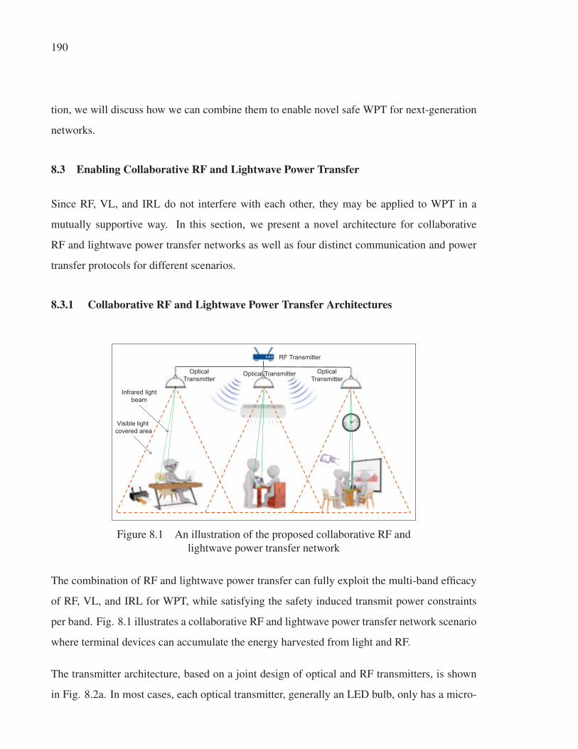
190

tion, we will discuss how we can combine them to enable novel safe WPT for next-generation

networks.

8.3 Enabling Collaborative RF and Lightwave Power Transfer

Since RF, VL, and IRL do not interfere with each other, they may be applied to WPT in a

mutually supportive way. In this section, we present a novel architecture for collaborative

RF and lightwave power transfer networks as well as four distinct communication and power

transfer protocols for different scenarios.

8.3.1 Collaborative RF and Lightwave Power Transfer Architectures


Infrared light beam

RF Transmitter

Optical Transmitter

Optical Transmitter

Optical Transmitter

Figure 8.1 An illustration of the proposed collaborative RF and

lightwave power transfer network

The combination of RF and lightwave power transfer can fully exploit the multi-band efficacy

of RF, VL, and IRL for WPT, while satisfying the safety induced transmit power constraints

per band. Fig. 8.1 illustrates a collaborative RF and lightwave power transfer network scenario

where terminal devices can accumulate the energy harvested from light and RF.

The transmitter architecture, based on a joint design of optical and RF transmitters, is shown

in Fig. 8.2a. In most cases, each optical transmitter, generally an LED bulb, only has a micro-

191

controller. Therefore, all computational tasks are processed at the RF transmitter, which is

often equipped with a powerful digital baseband unit.

The proposed receiver architecture is shown in Fig. 8.2b. In this architecture, the photodetector

is responsible of receiving both data and energy from the light which is then conveyed to an

alternating current (AC)-to-direct current (DC) separator in order to extract the DC component

from the light signals for the EH purpose. The separation can be performed in the time domain

or the power domain Diamantoulakis et al. (2018) and will be further described in Subsection

III.B. Moreover, RF signals, received from antennas, are split into two parts for information

decoding (ID) and EH. The part for ID is conveyed to the information receiver, while the one for

EH is directed to the EH unit where it is converted to DC form. Based on the harvested energy

from both RF and light and concurrent energy consumption, the energy management module

decides either to draw energy from the storage or convey excessive energy to the storage for

future use.

Internet

Wired Connection


Infrared light beam

Mobile Phone

Optical Transmitter

RF Transmitter

a) Transmitter architecture

Photodetector Antenna

AC-DC separator

Information receiver

Energy Management Storage

DC

AC

Splitter

RF energy harvester

AC AC

DC

b) Receiver architecture

Figure 8.2 Proposed transceiver design

8.3.2 Information and Power Transfer Protocols

Indeed, there are many possible combinations of using VL, IRL, and RF according to network

requirements. However, to maximize total power transfer performance while maintaining in-

192

formation transmission, our idea is to allocate the primary function of delivering information

and power to IRL, while the RF and the VL act as complimentary wireless power sources. It

can be explained by that IRL are able to provide significantly higher data rates than RF Pathak

et al. (2015). Additionally, the IRL band is more convenient than the VL band for transferring

energy because there are no constraints on consistent lighting in covered areas.

Protocol for the case of transmit power efficiency

(c)

Antenna

Energy (IRL)

Information & Energy & Illumination (VL)

Energy (RF)

Photodetector

Antenna

Protocol for the case of dimmed light

Photodetector Photodetector

Power splitting-based collaborative protocol

Time switching-based collaborative protocol

(b) (a) (d)

Photodetector

Antenna

Adjustable – controlled at the transmitter side Fixed – controlled at the transmitter side

Max Information (IRL) Energy (IRL) Min Energy (IRL)

Energy (RF)

Energy & Illumination (VL)

Information (IRL) Energy (IRL)

Energy (RF)

Max Information (VL) Min Energy & Illumination (VL)

Energy & Illumination (VL)

Antenna Energy (RF)

Information & Energy (IRL)

Figure 8.3 Information and power transfer protocols

In this context, motivated by the fact that the ID and EH performances can be managed in the

time and power domains, we first introduce two preliminary protocols, namely (a) and (b), as

follows.

Protocol (a): A power splitting-based collaborative protocol is shown in Fig. 8.3a, where

the RF only deliver energy, IRL conveys both information and energy, and VL maintains the

illumination in the served area and also contribute to EH performance. In this context, AC and

DC-biased components of the IRL signals determine the ID and EH performance, respectively.

Thus, managing the ID and EH performances can be achieved by adjusting the ratio between

the AC and DC powers.

Protocol (b): The IRL carries both information and power whereas the RF and VL convey

energy and illumination, respectively. This protocol is quite similar to protocol (a); however,

the management of the ID and EH associated to the IRL relies on time switching as shown in

Fig. 8.3b. In this context, the time frame is divided into two time-slots for information trans-

mission and power transfer, where the performances of information and energy are maximized,

193

respectively. Particularly, since IRL signals always include a DC-biased component; the light

energy can also be harvested in the time-slot dedicated to information transmission.

Furthermore, on this basis of protocols (a) and (b), we then present two more protocols (c)

and (d) to address the specific cases where the served areas have strong background light and

dimmed light, respectively, in the following.

Protocol (c): This protocol, presented in Fig. 8.3c, is designed for the case of transmit power

efficiency. The main motivation behind this protocol is due to the fact that although IRL can

deliver data at very high rates as VL, it consumes additional transmit power. However, as

mentioned, no extra transmit power needed from the lighting system for VL to convey either

information or energy. Hence, in protocol (c), we propose releasing IRL from the task of

information transmission. More specifically, IRL and RF is in charge of transferring power

while VL is responsible of delivering information, power, and proper illumination by using

either the similar power-splitting or time switching manner given in protocols (a) and (b).

Protocol (d): In contrast with protocol (c), this protocol addresses the scenario of dimmed

light in the served areas, e.g., a bedroom during rest time. The use of VL, in this case, is set in

a dimmable configuration that only focuses on maximizing ID performance with low-intensity

light. This is mainly due to the fact that although the light intensity can be enough to ensure a

reasonable data rate, it might be insufficient for harvesting energy. In this protocol, IRL and RF

play a complementary role to improve the ID or EH performance whenever necessary. Also,

IRL can be handled by either the power-splitting or time switching manner.

Note that in the proposed protocols, the ratio between AC and DC components and the RF

power-splitting factor can be optimized according to various requirements of the network.

8.3.3 Performance of Collaborative RF and Lightwave Power Transfer

We simulate a network consisting of a four-antenna RF transmitter, an optical transmitter, and

three single-antenna terminal deivces equipped with a solar pannel.

194

First, in order to visualize the safety level of the standalone RF WPT, a heat map of RF radiation

with respect to transmit power levels is shown in Fig. 8.4. In this simulation, the channel model

is subjected to the Rician fading with the Rician factor equal to 6 dB and the pathloss exponent

equal to 2.6. The devices are 4 meters far from the RF transmitter. For simplicity, maximal

ratio transmission (MRT) beamformer is used and the transmit power is equally allocated to

each device. According to the IEEE C95.1-2005 Standard, there is a SAR limit applied on

a person with 60 kg body mass which implies that only 13.3 mW EH rate can be beamed

towards the person. On this basis, in Fig. 8.4, the green areas indicate the safe zones for a

person. In practice, the safe zone might be rather small because of the existence of numerous

RF transmitters.

Distance (m)2 3 4 5 6 7 8

Tran

smit

Pow

er (d

Bm)

11

12

13

14

15

16

17

18

19

20

5

10

15

20

25

30

35

40

Beamedpower (mW)

Figure 8.4 Heat map of the RF radiation

As observed in Fig. 8.5a, VL and IRL can offer a much higher data rate than RF. Never-

theless, RF outperforms VL when considering the EH performance. Further, the achievable

performance of the four proposed protocols is depicted in Fig. 8.5b. According to LIGHTS

transmitter Lig, the IRL can be used to transfer watts of energy. However, in our application,

we consider the case of IoT devices where only milliwatts are harvested. In general, the com-

bined use of RF, VL, and IRL expands the rate-energy region significantly compared to the

sole use of either of the three resources. In Fig. 8.5b, the RF transmit power is reduced to 16

dB, implying a wider safe zone. However, the achievable EH of any protocol still outperforms

195

the EH of any individual approaches in Fig. 8.5a. In fact, the collaborative RF and lightwave

power transfer approach allows us to reduce the RF radiation while maintaining a decent EH

performance.

EH Rate (mW)0 5 10 15 20 25 30 35

Rat

e (b

its/H

z/s)

0

5

10

15

20

25

30

35

40

Power Splitting - VLTime Switching - VLPower Splitting - RFTime Splitting - RFPower Splitting - IRLTime Switching - IRL

a) Rate-energy region of each approach

EH Rate (mW)15 20 25 30 35 40 45

Rat

e (b

its/H

z/s)

0

10

20

30

40

50

60

70

Protocol (a)Protocol (b)Protocol (c)Protocol (d)

b) Rate-energy region of the proposed protocols

Figure 8.5 Scenarios of collaborative RF and lightwave power transfer

8.4 Future Research Opportunities

Since RF, VL, and IRL are complementary to each other, their combination can be applied to

many interesting applications in next-generation networks. In the following, we discuss some

future research opportunities.

8.4.1 Indoor Applications

8.4.1.1 Secure Wireless Powered Communication Networks

Beside the benefits of data rate, wireless energy transfer, and illumination; the applications of

the proposed collaborative approach, in nature, can also offer high security at the physical layer

of wireless networks. In other words, the combination of RF, VL, and IRL can be extensively

exploited to design new secure WPT scenarios to better protect information while transfering

data and wireless energy to devices. More specifically, it is motivated due to the fact that since

196

light cannot pass through opaque structures, the information it carries is secured from users

in other rooms or buildings. However, even though security is one of the main advantages of

OWC, dealing with the circumstance when eavesdroppers exist in the covered network area,

i.e., in the same room, is challenging. For instance, assume that eavesdroppers are able to

detect optical and RF signals. If the eavesdroppers are passive, the design of angle-diversity

optical transmitters with color allocation may help improve the network security, whereas RF

can play a role as artificial noise to decrease the eavesdropping performance while enhancing

the EH performance at the device. If the eavesdroppers are active and jam the network using

either RF or IRL (they may not use VL to jam the network since this manner will be able

to reveal their position), the network may use VL for secure communications while jamming

back the eavesdropper using RF and IRL. Additionally, as a consequence, the EH performance

is improved.

8.4.1.2 E-Healthcare

With the development of ICT, doctors can diagnose patients remotely. Thus, data transferred

from medical devices to the doctors should be accurate and timely because it might be crit-

ical to the lives of patients. The use of the lightwave for downlink can replenish energy for

medical or security devices such as handheld medical instruments, sensors, and smart locks

for health monitoring, and indoor localization. Indeed, this technology is a promising candi-

date for E-Healthcare, particularly in Telemedicine and Mobile Health (mHealth) applications

where patients can be connected with doctors and nurses in hospitals, at home, or anywhere

through one secure platform. Further, in these indoor applications, one of the main challenges

is providing high quality services while accounting for human eye safety regulations carefully

and maintaing consistent illumination in served areas.

197

8.4.2 Outdoor Applications

8.4.2.1 Unmanned aerial vehicles

In a disaster situation, such as an earthquake, providing continuous wireless communication is

vital for rescuing victims. In such situations, unmanned aerial vehicles (UAVs) could act as

a relay to convey information as well as to recharge devices over the air. A group of UAVs

can maintain communication and simultaneously recharge some devices, while searching for

victims in devastated buildings. In this hazardous circumtance, RF can be used to provide

continuous transmission for alert and command signals, which are not in need of high data

rate communication. Otherwise, lightwave is employed. Regarding wireless power transfer, in

the presence of LoS transmission, since narrow light beams can be created more conveniently

than narrow RF beams, the lightwave power transfer is preferred. Otherwise, RF is a more

suitable option. In this scenario, optimizing the position of the group of UAVs to improve

energy transfer efficiency is one of the most crucial challenges. Further, the health safety of

victims and rescue staffs should be guaranteed while delivering wireless power.

8.4.2.2 Underwater Communication and Power Transfer

While RF is an efficient approach for terrestrial communications, its use for underwater com-

munications faces many difficulties due to dramatic absorption losses. Generating RF signals

for underwater communications requires a considerable antenna size and a tramendous trans-

mit power, namely in hundreds of Watts, to achieve a 100 Mbps data rate. Further, the use of

RF for wireless power transfer is very challenging. On the other hand, narrow light beams can

be generated at a low cost and only need several Watts to achieve Gbps data rates. Therefore,

lightwave outperforms RF for underwater applications. However, this scenario might entail

a big challenge in terms of dealing with pointing errors due to bore-sight and jitter effects to

maintain a reasonable EH performance under when both transmitters and receiver are moving.

Hence, a hybrid scheme, where lightwave is used to transmit power and information at high

data rates over shorter range whereas RF is employed to send command and control signals

198

(i.e., not requiring high data rates) over the longer range, is a promising future direction for

this field.

8.5 Conclusion

In this article, we presented a brief overview of RF and optical power transfer techniques. Fur-

thermore, we introduced a framework for collaborative RF and lightwave power transfer. In

this regard, we developed a transceiver architecture suitable for hybrid RF and optical WPT.

Moreover, four communication and power transfer protocols for distinct scenarios were pro-

posed and challenged through simulations. We showed that supplemental performance gains

can be achieved by intelligently combining RF and lightwave technologies. Finally, several

future research directions have been highlighted to foster continuous advancement in this area.

It is firmly believed that this will become a fruitful research topic in the very near future. We

hope this article will inspire future research on this topic.

CONCLUSION AND RECOMMENDATIONS

9.1 Conclusion and Learned Lessons

Contemporarily, the world has witnessed the explosive development of ICT where 5G and IoT

are the key technologies. Due to the explosive progress of smart devices, such as Android and

Apple mobile phones, and the success of social networks, such as Instagram and Facebook, the

demands of heterogeneous wireless communication services have been exponentially increas-

ing. Nevertheless, generating sufficient power to supply ICT will produce carbon footprint

and then pollute the environment. For example, the electricity consumption by Facebook is

equivalent to by New York city. Also, in 2012, the CO2 emission in Quebec is 78.3 metric tons

carbon dioxide equivalent (Mt CO2 eq.) and is expected that the emissions achieve 20% below

1990 levels by 2020 Can (2015). Particularly, the ICT industry, one of the topics gaining the

top-most priority identified by the government of Quebec, generates a significant amount of

CO2. Indeed, the energy cost and CO2 emissions have been promptly growing due to the ICT

network operation. The aim to future green networks is not only an emerging issue in Quebec,

but also a global trend towards re-greening the world.

Over past few years, green radio communication has attracted much research work on en-

ergy saving to reduce the footprint from the ICT. Indeed, regreening future networks can be

identified as a crucial element in the action dealing with the climate change because it can

facilitate substantial cuts in global greenhouse gas emissions. Generally speaking, this disser-

tation focuses on four aspects: (i) minimizing power consumption, (ii) extending the lifetime

of wireless devices, (iii) exploiting available green natural resources and recyling RF and in-

door light signals in order to reduce carbon footprint, (iv) reducing electromagnetic pollution

to protect human health. In this vein, various resource allocation approaches for future green

wireless networks have been studied. To achieve all the aspects simultaneously, this thesis pro-

200

posed promising schemes to optimally manage and allocate resources in future networks. To

be specific, the thesis contributions are summarized as follows:

- In Chapter 2, we proposed the utilization of the TR technique in femtocell networks and de-

signed a new efficient power allocation scheme for HetNets where the backhaul connection

provides only an insufficient capacity for signaling exchange. Numerical results confirm a

siginificant transmit power saving in femtocell working environments.

- Chapter 3 presented an overview of some promising trends in future green networks. Ac-

cording to the principles of EH techniques, various concepts such as HetNet, mm-wave,

and IoT networks, have been considered. In particular, we concentrated on a promising ar-

chitecture: the green RF-WPT, which plays a vital role as a bridge between natural energy

resources and smart energy-hungry devices.

- Chapter 4 proposed an innovative integrated information and energy receiver architecture

based on the AC computing methodology. It was shown that the proposed architecture not

only improves the computational ability of IoT devices but also the energy efficiency.

- Chapter 5 introduced a novel approach for allocating resources in SWIPT systems under a

nonlinear EH model, where various crucial requirements related to the power consumption

minimization, RF EH performance and the effect of calibration error, need to be concur-

rently operated. Thus, the algorithms and the closed-form solutions to tackle these problems

were provided. In order to highlight the effectiveness of our work, the proposed scheme was

then compared with existing benchmarks and baseline.

- Chapter 6 proposed a novel collaborative RF and lightwave resource management design

for hybrid RF/VLC ultra-small cell networks. Further, we derived optimal solutions and a

simple closed-form suboptimal solution to aid the solving process. It was demonstrated that

the collaborative scheme significantly enhances the overall power efficiency and reduces RF

pollution while supporting an appropriate illumination in the area.

201

- In Chapter 7, we proposed the employment of lightwave power transfer in FL-based wire-

less networks. In this vein, we introduced a scheme to handle the network power efficiency.

It was indicated that the proposed scheme can sufficiently recharge energy for the terminal

devices to execute FL tasks.

- Chapter 8 presented a framework for collaborative RF and lightwave power transfer. In

more detail, we developed a transceiver architecture suitable for hybrid RF and optical

WPT. Furthermore, four protocols to handle communication and power transfer for different

scenarios were introduced through simulations. It was shown that substantial performance

gains can be attained by cleverly combining RF and lightwave technologies.

This dissertation aims at proposing novel solutions with the purpose of satisfying all the tech-

nical, economic, and environmental perspectives of future networks. Particularly, according to

the conducted research, there are some interesting learned lessons as follows:

- Interference management is the key solution to handle the system performance of wire-

less information transmission and power transfer networks. It is because wisely exploiting

interference can improve the EH performance significantly.

- Solely using RF signals may be not sufficient to power wireless devices due to the propa-

gation loss, RF-DC conversion efficiency, and safety threshold.

- Optimal solutions are important but suboptimal ones with low-complexity are more necces-

sary to wireless networks.

- AI-powered wireless networks where the network could make correct decisions automati-

cally would be the future.

202

9.2 Recommendations: Energy Transfer and Harvesting for 6G networks

According to Saad, W., Bennis, M. & Chen, M. (2019), 6G could be the first cellular network

generation that can realize wirelessly recharging energy for terminal devices. Since WPT tech-

nology is ripening, it is believable to envision that 6G BSs would be able to provide essential

power transfer for devices. Hence, some potential directions for future research are discussed

below.

9.2.1 Mobile Energy Internet

It is well-known that the evolution from Fixed Internet to Mobile Internet on the 2G to 5G

platforms has actualized wireless information propagation and determines the barrier of last-

kilometer information transmission. Thus, inspired by this success, the concept of Mobile

Energy Internet has been introduced in Liu, M., Xiong, M., Deng, H., Liu, Q., Wu, J. & Xia, P.

(2018) to overcome the boundaries of fixed power transfer with the conventional power grid.

This approach promises to solve the issue of last-meter power transfer and transition power

delivery into a mobile realm.

9.2.2 Deep Learning for Resource Allocation in Green Wireless Communications

An innovative deep learning-based approach for wireless resource management is promising.

The main idea behind it is to handle a given optimization algorithm as a “black box” and then

attempt to determine its input/output relation by adopting a deep neural network (DNN). The

key improvement is that the DNN has distinguished real-time computational efficiency com-

pared with conventional iterative optimization algorithms. In more detail, its run-time stage

excludes numerical optimization tasks and only requires some basic calculations, such as ma-

trix multiplication/addition. If the training stage can produce an approximator of the algorithm

which is accurately sufficient, then simple real-time resource allocation is conceivable.

203

9.2.3 Reinforcement Learning for Self-Organizing Green Wireless Communications

Self-organization is one of the primary features of future cellular networks which is becoming

more heterogeneous and densified through the form of small cells. In this vein, reinforcement

learning (RL) is a promising solution to support this feature. In principle, RL is a learning

strategy where an agent can repeatedly make decisions, analyze the outcomes, and hence au-

tomatically modify its policy to achieve a specific goal. One of the main advantages of RL

compared with supervised learning methods is that there is no need for correct input/output

data in the training phase.

9.2.4 New Green Sources: Invisible Light

The utilization of invisible light, such as infrared light, as a supplementary energy and informa-

tion source will be very promising. Regulating the invisible light band might be more adaptable

than the visible one since it does not influence illumination. Nonetheless, resource allocation

designs require to thoroughly consider human eye safety standards.

APPENDIX I

APPENDIX OF CHAPTER 2

1. Proof of Lemma 1

To solve this problem OP1, we start with introducing a new parameter for the objective function

as follows

N1

∑j=1

⎛⎝ N0

∑n=1

∥∥∥∥∥M1

∑i=1

gi j ∗h10in

∥∥∥∥∥2

p1j

⎞⎠= ηηηT p1, (A I-1)

where ηηη are defined in Lemma 1.

Next, the expression of SINR1j in (2.14) can be re-written as

SINR1j

(L, p1,

{g1

i j}M1,N1

i=1, j=1,P(cross)

1j

)(A I-2)

=

⎛⎝∣∣∣∣(

M1

∑i=1

gi j ∗h1i j

)[L]∣∣∣∣2

− γ1j

2L−1

∑l=1l �=L

∣∣∣∣(

M1

∑i=1

gi j ∗h1i j

)[l]∣∣∣∣2⎞⎠ p1

j

P(co)1j +P(cross)

1j +‖nF [β ]‖2

.

Accordingly, in form of matrix-vector notation, the OP1 can be formulated as follows

OP1−1: minp1

ηηηT p1

s.t. p1 � DBp1 + z,(A I-3)

in which, the structures of D, B, and z are defined in Lemma 1.

Considering the objective function of OP1−1, it is a fact that

ηηηT p1 = ‖ηηη‖Tr(diag(ηηη)p1

), (A I-4)

206

where ηηη is the normalized form of ηηη which can be computed as ηηη =ηηη‖ηηη‖ .

On this basis, we aim at deriving the constraint of OP1−1 as a function of(diag(ηηη)p1

). After

some manipulations, the constraint can be shown in a new equivalent formulation as

p1 � DBp1 + z

⇔ diag(ηηη)p1 � diag(ηηη)D(B◦ (ηηη−11T

N1×1))

diag(ηηη)p1 + z. (A I-5)

Hence, the OP1−1 can be re-formulated as

OP1−2: minp1

‖ηηη‖Tr(diag(ηηη)p1

)s.t. diag(ηηη)p1 � diag(ηηη)D

(B◦ (ηηη−11T

N1×1))

×diag(ηηη)p1 + z.

(A I-6)

Therefore, the closed-form expression of p�1 can be given by

p�1 = diag(ηηη)−1[IN1−diag(ηηη)D

(B◦ (ηηη−11T

N1×1))]−1 z. (A I-7)

Relying on Perron-Frobenius theory, the optimal value p�1 is guaranteed to be a nonnegative

vector if and only if the spectral radius of diag(ηηη)D(

B◦ (ηηη−11TN1×1)

)is less than unity.

Furthermore, in a special case where η1 = η2 = ... = ηN1= η , the above problem can be

written in a simplified form as

OP1−3: minp1

ηITN1

p1

s.t. p1 � DBp1 + z.(A I-8)

207

Then, the optimal solution of OP1−2 can be given as

p�1 = (I−DB)−1 z. (A I-9)

One can see that the result of (A I-9) is in agreement with that of the work in Chandrasekhar

et al. (2009). In final, the proof is completed.

2. Proof of Lemma 2

According to (2.58), we can write down that

mine1

i j∈F 1i j

∣∣∣∣∣M1

∑i=1

(gi j ∗h1i j)[L]

∣∣∣∣∣2

= mine1

i j∈F 1i j

∣∣∣∣M1

∑i=1

(∥∥∥h1i j

∥∥∥2+(e1

i j)Hh1

i j

)∣∣∣∣2

M1

∑i=1

∥∥∥h1i j

∥∥∥2

(a)=

∣∣∣∣M1

∑i=1

(∥∥∥e1i j

∥∥∥2(

1−√ψψ

))∣∣∣∣2

M1

∑i=1

∥∥∥h1i j

∥∥∥2. (A I-10)

The equality in (a) is due to the fact that the quantity of

(∥∥∥h1i j

∥∥∥2+(e1

i j)Hh1

i j

)reaches the

minimum if and only if e1i j =−

√ψh1i j.

Next, by substituting e1i j =−

√ψh1i j to (2.59), we can obtain the following derivation

∥∥e1i j∥∥2

=ψ

(1−√ψ)2

∥∥h1i j∥∥2

. (A I-11)

Thus, we infer that

mine1

i j∈F 1i j

∣∣∣∣∣M1

∑i=1

(gi j ∗h1i j)[L]

∣∣∣∣∣2

=

M1

∑i=1

∥∥∥h1i j

∥∥∥2

(1−ψ)2. (A I-12)

208

On the other hand, the estimated signal power can be given as

∣∣∣∣∣M1

∑i=1

(gi j ∗ h1i j)[L]

∣∣∣∣∣2

=M1

∑i=1

∥∥h1i j∥∥2. (A I-13)

Accordingly, the worst-case lower-bound of signal power component can be constituted as

Pl(sig)1j =

∣∣∣∣∣M1

∑i=1

(gi j ∗ h1i j)[L]

∣∣∣∣∣2

p1j(

1−√ψ)2. (A I-14)

This completes the proof of Lemma 2.

3. Proof of Lemma 3

We consider the worst-case upper-bound of∥∥∥gi j ∗h1

i j

∥∥∥2for simplicity. To investigate a tighter

upper-bound than the value suggested in Beckner (1975); Young (1912), we introduce a novel

approach in which we start with letting h1i j be a virtual channel, and we aim at investigating the

optimal value h�1i j that makes

∥∥∥gi j ∗ h1i j

∥∥∥2achieve maximal quantity. Accordingly, the problem

becomes

maxh1

i j

∥∥gi j ∗ h1i j∥∥2

s.t.∥∥h1

i j∥∥2 ≤ max

e1i j∈F 1

i j

∥∥h1i j∥∥2

. (A I-15)

As observed, the problem (A I-15) is hard to solve directly due to the convolution operator.

Thus, we factorize (A I-15) into two steps. In the first step, we let Gi j to be a (2L− 1)× L

Toeplitz matrix form of gi j, i.e. (2.65)

209

Additionally, we let ΦΦΦ1i j =

h1i j√

maxe1

i j∈F 1i j

∥∥∥h1i j

∥∥∥2. Based on the representation of convolution with

Toeplitz matrix form, the above problem can be equivalently re-formulated as

maxΦΦΦ1

i j

∥∥∥∥∥(√

maxe1

i j∈F 1i j

∥∥∥h1i j

∥∥∥2Gi j

)ΦΦΦ1

i j

∥∥∥∥∥2

s.t.∥∥ΦΦΦ1

i j∥∥2 ≤ 1. (A I-16)

The closed-form derivation of optimal solution ΦΦΦ�1i j can be obtained by computing the orthonor-

mal eigenvector corresponding to the largest eigenvalue of the matrix

(Gi j

(Gi j

)Hmax

e1i j∈F 1

i j

∥∥∥h1i j

∥∥∥2)

.

Since the norm of ΦΦΦ�1i j is equal to 1, to make a fair normalization, we devise that

h�1i j =

(ΦΦΦ�1

i j) ∥∥∥h1

i j

∥∥∥(1−√ψ

) , (A I-17)

where h�1i j is the optimal value regarding to the achievement the maximum of

∥∥∥gi j ∗ h1i j

∥∥∥2, and

maxe1

i j∈F 1i j

∥∥∥h1i j

∥∥∥2=

∥∥∥h1i j

∥∥∥2

(1−√ψ

)2.

Therefore, we can obtain a new boundary from (A I-17) as

maxe1

i j∈F 1i j

∥∥∥∥∥M1

∑i=1

gi j ∗h1i j

∥∥∥∥∥2

(A I-18)

=M1

∑i=1

∥∥gi j ∗ h�1i j∥∥2

+

∣∣∣∣∣∣M1

∑i=1

M1

∑i=1i′ �=i

(gi j ∗ h�1

i j)H(

gi′ j ∗ h�1i′ j

)∣∣∣∣∣∣ .

Thus, the proof of Lemma 3 is completed.

APPENDIX II


1. Proof of Lemma 1

We assume that there is a value of φ0 such that

θ(1−φ0)Γ

=ε

Γφ0= Ξ. (A II-1)

Next, by increasing φ0 with a (a > 0 and 0 < a+φ0 < 1), it can be observed that

max

{θ

Γ(1− (φ0 +a)),

εΓ(φ0 +a)

}=

θΓ(1− (φ0 +a))

> Ξ. (A II-2)

Furthermore, by decreasing φ0 with b (b > 0 and 0 < φ0−b < 1)

max

{θ

Γ(1− (φ0−b)),

εΓ(φ0−b)

}=

εΓ(φ0−b)

> Ξ. (A II-3)

Thus, (A II-2) and (A II-3) imply that either increasing φ or decreasing φ results in a scale up

of the objective function of OP3. Therefore, φ0 is the optimal solution of OP3 (i.e., φ� = φ0),

and the proof of Lemma 1 is completed.

APPENDIX III


1. Proof of Lemma 1

To compute an approximation for (5.38), we begin with considering the simplified form (setting

G = N1 = 1) as follows

Pr

(−p1

1

∣∣(ννν11)

T h11

∣∣2 ≥ θ 11

(ρ11 −1)

)≤ 1−α�1

1 . (A III-1)

Following the one-sided Chebyshev-inequality, we have

Pr(−p1

1

∣∣(ννν11)

T h11

∣∣2 +E

[p1

1

∣∣(ννν11)

T h11

∣∣2]≥ t)

≤ 1

1+ t2/var[

p11

∣∣(ννν11)

T h11

∣∣2] , (A III-2)

where t ≥ 0. By taking

t =θ 1

1

(ρ11 −1)

+E

[p1

1

∣∣(ννν11)

T h11

∣∣2] , (A III-3)

one can see that the expression (A III-1) is equivalent to the one (A III-2). On this basis, we

obtain

Pr

(−p1

1

∣∣(ννν11)

T h11

∣∣2 ≥ θ 11

(ρ11 −1)

)

≤var[

p11

∣∣(ννν11)

T h11

∣∣2]

var[

p11

∣∣(ννν11)

T h11

∣∣2]+( θ 11

ξ 11 (ρ

11 −1)

+E

[p1

1

∣∣(ννν11)

T h11

∣∣2])2. (A III-4)

214

As a result, the inequality

var[

p11

∣∣(ννν11)

T h11

∣∣2]

var[

p11

∣∣(ννν11)

T h11

∣∣2]+(

θ 11

(ρ11 −1)

+E

[p1

1

∣∣(ννν11)

T h11

∣∣2])2

≤ 1−α�11 . (A III-5)

implies the probability inequality given in (A III-1).

Additionally, since t ≥ 0, the expression in (A III-5) can be re-written by

√var[

p11

∣∣(ννν11)

T h11

∣∣2](1/(1−α�11 )−1

)≤ E

[p1

1

∣∣(ννν11)

T h11

∣∣2]+ θ 11

(ρ11 −1)

. (A III-6)

By generalizing (A III-1)-(A III-6),

√√√√(1/(1−α�gn )−1

) G

∑g′=1

Ng

∑n′=1

var[|(νννg′

n′)T hg

n|2](pg′

n′)2

≤G

∑g′=1

Ng

∑n′=1

E

[∣∣∣(νννg′n′)

T hgn

∣∣∣2] pg′n′+

θ gn

(ρgn −1)

. (A III-7)

Also, it is known that

√√√√ G

∑g′=1

Ng

∑n′=1

var[|(νννg′

n′)T hg

n|2](pg′

n′)2

≤G

∑g′=1

Ng

∑n′=1

√var[|(νννg′

n′)T hg

n|2]

pg′n′ . (A III-8)

215

Thus, (A III-7) can be approximated as follows

G

∑g′=1

Ng

∑n′=1

√(1/(1−α�g

n )−1)

var[|(νννg′

n′)T hg

n|2]

pg′n′

≤G

∑g′=1

Ng

∑n′=1

E

[∣∣∣(νννg′n′)

T hgn

∣∣∣2] pg′n′+

θ gn

(ρgn −1)

. (A III-9)

This completes our proof.

2. Proof of Lemma 2

To calculate E

[∣∣∣(νννg′n′)

T hgn

∣∣∣2], it is useful to represent it into a formulation regarding the trace

operator as follows

E

[∣∣∣(νννg′n′)

T hgn

∣∣∣2]= E

[tr(

Vg′n′h

gn(h

gn)

H)]

. (A III-10)

Due to the facts that (i) both E [.] and tr are linear operators and (ii) hgn ∼ C N (ug

n,σ2calU

gn),

where Ugn = diag{|ug

n[1]|2, ..., |ugn[M]|2}, we can derive

E

[tr(

Vg′n′h

gn(h

gn)

H)]

= tr(

Vg′n′E[hg

n(hgn)

H])= tr(

Vg′n′U

gnσ2

cal

)+(ug

n)HVg′

n′ugn. (A III-11)

On the other hand, one can observe that computing the variance of∣∣∣(νννg′

n′)T hg

n

∣∣∣2 is quite compli-

cated. Fortunately, based on the work in [Chapter 2, ?], after some manipulations, the cumulant

generating function (CGF) of∣∣∣(νννg′

n′)T hg

n

∣∣∣2 can be given by

CGFk

(|(νννg′

n′)T hg

n|2)= (k−1)!

[tr(

Vg′n′U

gnσ2

cal

)k

+k(ugn)

HVg′n′(

σ2calU

gnVg′

n′)k−1

ugn

]. (A III-12)

216

Particularly, by setting k = 2, the variance of∣∣∣(νννg′

n′)T hg

n

∣∣∣2 can be shown as

var

[∣∣∣(νννg′n′)

T hgn

∣∣∣2]= tr(

Vg′n′U

gnσ2

cal

)2

+2σ2cal(u

gn)

HVg′n′UVg′

n′ugn. (A III-13)


3. Proof of Lemma 4

First, we consider constraint (5.52b). According to (5.39), the constraint can be re-expressed

as

(μμμgn−υυυg

n)T a(σ2

0 +σ2

1

ρ)≥ θ g

n

(1−ρ), (A III-14)

where

a = (I−Lϒϒϒ)−1ΔΔΔ1NG, (A III-15a)

μμμgn = [μ1g

1n ...μGgNn ]

T , (A III-15b)

αgn = (1/(1−α�g

n )−1) , (A III-15c)

υυυgn = [

√αg

n υ1g1n ...

√αg

n υGgNn ]

T . (A III-15d)

By inverting both sides, we can obtain the derivation as below

ρρ(μμμg

n−υυυgn)T aσ2

0 +(μμμgn−υυυg

n)T aσ21

≤ (1−ρ)θ g

n. (A III-16)

After some manipulations, the constraint can be further transformed into a second-order in-

equation as

(μμμgn−υυυg

n)T aσ2

0 ρ2−κgn ρ− (μμμg

n−υυυgn)

T aσ21 ≤ 0, (A III-17)

217

in which,

κgn = (μμμg

n−υυυgn)

T a(σ20 −σ2

1 )− θ gn . (A III-18)

In particular, according to (A III-14), it can be induced that (μμμgn−υυυg

n)T a≥ 0 to make the prob-

lem feasible. This yields that (A III-17) is a convex quadratic constraint Boyd & Vandenberghe

(2004). In other words, constraint (5.52b) has been transformed into a convex formulation.

Second, we analyze the convexity of the objective function of problem (5.52). Taking (5.45),

(5.50), and (5.51) into account, it can be evaluated that since matrix (I−Lϒϒϒ)−1ΔΔΔ is positive

element-wise Bambos et al. (2000), Λg,n(1/ρ) is convex. Thus, the objective function of prob-

lem (5.52) can be seen as a summation of convex functions. Therefore, the objective function

is convex.

Based on the above discussion, it can be concluded that problem (5.52) is convex.

Next, since the objective function of problem (5.52) is non-increasing, the closed-form solution

can be given by

ρ� = min1≤n≤N1≤g≤G

⎧⎨⎩

κgn +√

(κgn )2 +4((μμμg

n−υυυgn)T a)2σ2

0 σ21

2(μμμgn−υυυg

n)T aσ20

⎫⎬⎭ . (A III-19)


APPENDIX IV


1. Proof of Proposition 1

For convenience, we use SNRsoi, j(B) to denote that the VLC SNR at any user is a function of B.

Our aim is to maximize the minimum of the VLC SNRs, i.e., max min SNRsoi, j(B).

Since SNRsoi, j(B) is an increasing function, inreasing B leads to increasing the VLC SNRs at all

the users. Thus, maximizing the minimum of VLC SNRs is equivalent to simply maximizing

the VLC SNR at the user with the worst VLC SNR, mathematically represented as

max min SNRsoi, j(B) = max SNRsoi, j(B), (A IV-1)

where j denotes the user with the worst VLC SNR.

Furthemore, according to (6.15b), there is a relationship between the VLC SNR and the VLC

EH. It can be seen that maximizing the VLC SNR implies minimizing the VLC EH. Hence,

we have

max SNRsoi, j(B) = min EHV LCj (B). (A IV-2)

Next, due to constraint (6.15b), reducing EHV LCj (B) is achieved by adding more EHRF

j . Gener-

ally speaking, increasing the RF EH reduces the contribution of the VLC EH, and increases

the achievable amount of the VLC SNRs. Therefore, the RF EH allocated to the user with

the worst VLC SNR determines the value of the minimum of the VLC SNRs, and therefore

determines B for all the users. This completes the proof.

220

2. Proof of Lemma 1

To demonstrate the rank-one issue, we can have some following expressions based on the

Karush-Kuhn-Tucker (KKT) condition as Boyd & Vandenberghe (2004)

I− γ jG j−ΞΞΞ j = 0, (A IV-3)

W jΞΞΞ j = 0, (A IV-4)

where γ j and ΞΞΞ j are dual variables associated with constraints (6.35b) and (6.35c), respectively.

On one hand, according to (6.35b), (6.35c), and (A IV-4), it is implied that W j �= 0. Thus, we

infer that

rank(ΞΞΞ j)≤MT −1. (A IV-5)

On the other hand, based on (A IV-3), we have

rank(ΞΞΞ j) = rank(I− γ jG j)≥MT −1. (A IV-6)

Taking (A IV-5) and (A IV-6) into account, it is clear that

rank(ΞΞΞ j) = MT −1. (A IV-7)

Next, in light of (A IV-4), the rank of W j can be calculated by

rank(W j)≤MT − rank(ΞΞΞ j). (A IV-8)

Since rank(W j) �= 0 due to W j �= 0, we conclude that

rank(W j) = 1. (A IV-9)

221


3. Proof of Lemma 2

The key to achieving a closed-form solution for problem (6.30) relies on dealing with constraint

(7.20). We recall the constraint as follows

fV0I j,G(B)ln(

1+I j,G(B)

ID

)≥ θ −EH�RF

j . (A IV-10)

Initially, we aim to transform the constraint into a simplified form of B greater than a constant.

Unfortunately, this is difficult to achieve. Then, deriving a closed-form optimal solution is

intractable. However, a closed-form suboptimal solution can be obtained by relaxing constraint

(7.20). Our method is presented as follows.

Since ID � I j,G(B) in practice, we can have an approximation as

ln

(1+

I j,G(B)ID

)≈ ln

(I j,G(B)

ID

). (A IV-11)

Thus, (A IV-10) becomes

I j,G(B)ln(

I j,G(B)ID

)≥

θ −EH�RFj

fV0, (A IV-12)

After some manipulations, I j,G(B) can be computed as

I j,G(B)≥θ −EH�RF

j

fV0W

(θ−EH�RF

jfV0ID

) (A IV-13)

222

where W (.) is the Lambert function. Accordingly, we have

B≥θ −EH�RF

j

3νNLEDVLED fV0W

(θ−EH�RF

jfV0ID

)O∑o

MI∑i

hoi, j

= ϒ. (A IV-14)

Accordingly, problem (6.30) becomes

minB

B (A IV-15a)

s.t.: B≥ ϒ, (A IV-15b)

IH + IL

2≤ B≤ IH . (A IV-15c)

As observed, the closed-form suboptimal solution can be computed as follows

B× = min{max{ϒ, IL}, IH} , (A IV-16)

A×soi, j = B−B×. (∀ j) (A IV-17)

Thus, our proof is completed.

REFERENCES

The European lighting standard – EN12464-1:2011. Light and lighting – Lighting of work

places – Part 1: Indoor work places.

LIGHTS Transmitter. Consulted at https://www.wi-charge.com/product_category/reference

-integrations/.

How to Harvest and Store Wind Energy. Consulted at http://www.ctmmagnetics.com/wind

-power-basics-how-to-harvest-and-store-wind-energy/.

Philips. All in 1 LED Lighting Solutions Guide. Consulted at PhilipsLumileds.com.

Google. Federated Learning: Collaborative Machine Learning without Centralized Training

Data. Consulted at https://ai.googleblog.com/2017/04/federated-learning-collaborative

.html.

IEC. (2001). Safety of laser products - Part 1: Equipment classification, requirements and

user’s guide.

IEEE. (2005). IEEE Standard for Safety Levels With Respect to Human Exposure to Radio

Frequency Electromagnetic Fields, 3 kHz to 300 GHz.

(2007). Extremely Low Frequency Fields, Environmental Health Criteria 238. Geneva,

Switzerland.

(2014). Green Power for Mobile. Consulted at https://www.gsma.com/mobilefordevelopment/

wp-content/uploads/2015/01/140617-GSMA-report-draft-vF-KR-v7.pdf.

CBC. (2015). How Canada’s provinces are tackling greenhouse gas emis-

sions. Consulted at http://www.cbc.ca/news/canada/how-canada-s-provinces-are

-tackling-greenhouse-gas-emissions-1.3030535.

(2019). Wysips Reflect. Consulted at https://sunpartnertechnologies.fr/en/objets-connectes/

produits/.

3GPP. (2009). Hardware calibration requirement for dual layer beamforming (Report n◦R1-

091794).

Agarwal, D., Chen, B.-C., Elango, P. & Wang, X. (2012, August). Personalized click shap-

ing through lagrangian duality for online recommendation. the 35th International ACMSIGIR Conference on Research and Development in Information Retrieval.

Agiwal, M., Roy, A. & Saxena, N. (2016). Next Generation 5G Wireless Networks: A Com-

prehensive Survey. IEEE Communications Surveys & Tutorials, 18(3), 1617 – 1655.

224

Ahmed, E., Eltawil, A. M. & Sabharwal, A. (2013). Self-interference cancellation with phase

noise induced ICI suppression for full-duplex systems. in Proc. IEEE Global Commun.Conf. (GLOBECOM), pp. 3384–3388.

Al-Fuqaha, A., Guizani, M., Mohammadi, M., Aledhari, M. & Ayyash, M. (2015). Internet

of Things: A Survey on Enabling Technologies, Protocols, and Applications. IEEECommunications Surveys & Tutorials, 17(4), 2347 – 2376.

Alippi, C. & Galperti, C. (2008). An Adaptive System for Optimal Solar Energy Harvesting

in Wireless Sensor Network Nodes. IEEE Transactions on Circuits and Systems, 55(6),

742–1750.

Americas, G. (2009). The benefits of son in LTE: Self-optimizing and selforganizing networks.

White Paper.

Amiri, R., Almasi, M. A., Andrews, J. G. & Mehrpouyan, H. (2019). Reinforcement Learning

for Self Organization and Power Control of Two-Tier Heterogeneous Networks. IEEETransactions on Wireless Communications. early access.

Ammar, Y., Buhrig, A., Marzencki, M., Charlot, B., Basrour, S., Matou, K. & Renaudin,

M. (2005, October). Wireless sensor network node with asynchronous architecture

and vibration harvesting micro power generator. Proc. of Joint sOc-EUSAI conference,

pp. 287–292.

Andrews, J., Claussen, H., Dohler, M., Rangan, S. & Reed, M. (2012). Femtocells: Past,

Present, and Future. IEEE Journal on Selected Areas in Communications, 30(3), 497–

508.

Arnon, S. (Ed.). (2015). Visible Light Communication. Cambridge University Press.

Ayyash, M., Elgala, H., Khreishah, A., Jungnickel, V., Little, T., Shao, S., Rahaim, M., Schulz,

D., Hilt, J. & Freund, R. (2016). Coexistence of WiFi and LiFi Toward 5G: Concepts,

Opportunities, and Challenges. IEEE Communications Magazine, 54(2), 64 – 71.

Bambos, N., Chen, S. C. & Pottie, G. J. (2000). Channel Access Algorithms with Active

Link Protection for Wireless Communication Networks with Power Control. IEEE/ACMTransactions on Networking, 5(8), 583–597.

Baraniuk, R. (2007). Compressive Sensing. IEEE Signal Processing Magazine, 24(4), 118 –

121.

Basnayaka, D. A. & Haas, H. (2017). Design and Analysis of a Hybrid Radio Frequency and

Visible Light Communication System. IEEE Transactions on Communications, 65(10),

4334 – 4347.

225

Beck, A., Ben-Tal, A. & Tetruashvili, L. (2010). A sequential parametric convex approxima-

tion method with applications to nonconvex truss topology design problems. Journal ofGlobal Optimization, 47(1), 29 – 51.

Beckner, W. (1975). Inequalities in Fourier analysis. Ann. of Math., 102(1), 159–182.

Belkhir, L. & Elmeligi, A. (2018). Assessing ICT global emissions footprint: Trends to 2040

& recommendations. Journal of Cleaner Production, 177, 448–463.

Bengtsson, M. & Ottersten, B. (2001). Optimal and Suboptimal Transmit Beamforming. CRC

Press.

Bennis, M., Giupponi, L., Diaz, E., Lalam, M., Maqbool, M., Strinati, E., De Domenico,

A. & Latva-aho, M. (2011). Interference management in self-organized femtocell net-

works: The BeFEMTO approach. Proc. of 2nd International Conference on WirelessCommunication, Vehicular Technology, Information Theory and Aerospace & ElectronicSystems Technology (Wireless VITAE), pp. 1–6.

Bi, S., Ho, C. K. & Zhang, R. (2014). Recent advances in joint wireless energy and information

transfer. Proc. IEEE Information Theory Workshop (ITW 2014), pp. 341–345.

Bi, S., Ho, C. & Zhang, R. (2015). Wireless powered communication: opportunities and

challenges. IEEE Communications Magazine, 53(4), 117–125.

Bjornson, E. & Jorswieck, E. (2013). Optimal resource allocation in coordinated multi-cell

systems. Foundations and Trends in Communications and Information Theory, 9(2-3),

113–381.

Bjornson, E., Jorswieck, E. A., Debbah, M. & Ottersten, B. (2014). Multiobjective Signal

Processing Optimization: The way to balance conflicting metrics in 5G systems. IEEESignal Processing Magazine, 31(6), 14 – 23.

Bobkov, S., Madiman, M. & Wang, L. (2011). Fractional generalizations of Young and Brunn-

Minkowski inequalities. Contemporary Mathematics, 545.

Bogachev & I., V. (2007). Measure Theory I. New York: Springer-Verlag.

Bonnefoi, R., Moy, C. & Palicot, J. (2018). Power Control and Cell Discontinuous Transmis-

sion Used As a Means of Decreasing Small-Cell Networks’ Energy Consumption. IEEETransactions on Green Communications and Networking, 2(6), 899 – 914.

Boshkovska, E., Ng, D. W. K., Zlatanov, N. & Schober, R. (2015). Practical Non-Linear Energy

Harvesting Model and Resource Allocation for SWIPT Systems. IEEE CommunicationsLetters, 19(12), 2082 – 2085.

226

Boshkovska, E., Ng, D. W. K., Zlatanov, N., Koelpin, A. & Schober, R. (2017). Robust

Resource Allocation for MIMO Wireless Powered Communication Networks Based on

a Non-linear EH Model. IEEE Transactions on Communications, 65(5), 1984 – 1999.

Bottner, H. & et al. (2004). New Thermoelectric Components Using Microsystem Technolo-

gies. Journal of Microelectromechanical Systems, 13(3), 414–420.

Bouzigues, M.-A., Siaud, I., Helard, M. & Ulmer-Moll, A.-M. (2013). Turn Back the Clock:

Time Reversal for Green Radio Communications. IEEE Vehicular Technology Magazine,

8(1), 49–56.

Boyd, S. & Vandenberghe, L. (2004). Convex Optimization. Cambridge University Press.

Buzzi, S., I, C.-L., Klein, T. E., Poor, H. V., Yang, C. & Zappone, A. (2016). A Survey of

Energy-Efficient Techniques for 5G Networks and Challenges Ahead. IEEE Journal onSelected Areas in Communications, 34(4), 697–709.

Caramia, M. & Dell’Olmo, P. (2008). Multi-objective management in freight logistics: Increas-ing capacity, service level and safety with optimization algorithms. Springer Science &

Business Media.

Carvalho, C. & Paulino, N. (2014). On the Feasibility of Indoor Light Energy Harvesting for

Wireless Sensor Networks. Procedia Technology, 17, 343–350.

Chandrasekhar, V., Andrews, J. G., Muharemovic, T., Chen, Z. & Gatherer, A. (2009). Power

control in two-tier femtocell networks. IEEE Transactions on Wireless Communications,

8(8), 4316–4328.

Chen, C., Basnayaka, D. A. & Haas, H. (2016a). Downlink Performance of Optical Attocell

Networks. IEEE/OSA J. Lightw. Technol., 34(1), 137 – 156.

Chen, F. & Zhang, Y. (2013). Sparse Hyperspectral Unmixing Based on Constrained lp - l2

Optimization. IEEE Geoscience and Remote Sensing Letters, 10(6), 1142 – 1146.

Chen, H. H., Li, Y., Jiang, Y., Ma, Y. & Vucetic, B. (2015). Distributed Power Splitting

for SWIPT in Relay Interference Channels Using Game Theory. IEEE Transactions onWireless Communications, 14(1), 410–420.

Chen, Y., Wang, B., Han, Y., Lai, H.-Q., Safar, Z. & Liu, K. R. (2016b). Why Time Reversal for

Future 5G Wireless? [Perspectives]. IEEE Signal Processing Magazine, 33(2), 17–26.

Chen, Z., Basnayaka, D. A. & Haas, H. (2017). Space Division Multiple Access for Optical

Attocell Network Using Angle Diversity Transmitters. IEEE/OSA J. Lightw. Technol.,35(11), 2118 – 2131.

227

Chiang, P., Guruprasad, R. B. & Dey, S. (2018). Optimal Use of Harvested Solar, Hybrid

Storage and Base Station Resources for Green Cellular Networks. IEEE Transactions onGreen Communications and Networking, 2(3), 707–720.

Chingoska, H., Hadzi-Velkov, Z., Nikoloska, I. & Zlatanov, N. (2016). Resource Allocation

in Wireless Powered Communication Networks With Non-Orthogonal Multiple Access.

IEEE Wireless Communications Letters, 5(6), 684 – 687.

Clerckx, B. & Bayguzina, E. (2016). Waveform Design for Wireless Power Transfer. IEEETransactions on Signal Processing, 64(23), 6313–6328.

Clerckx, B., Zhang, R., Schober, R., Ng, D. W. K., Kim, D. I. & Poor, H. V. (2019). Fundamen-

tals of Wireless Information and Power Transfer: From RF Energy Harvester Models to

Signal and System Designs. IEEE Journal on Selected Areas in Communications, 37(1),

4–33. Consulted at https://arxiv.org/abs/1803.07123.

Covic, G. A. & Boys, J. T. (2013). Inductive Power Transfer. Proceedings of the IEEE, 101(6),

1276–1289.

Diamantoulakis, P. D. & Karagiannidis, G. K. (2017). Maximizing Proportional Fairness in

Wireless Powered Communications. IEEE Wireless Communications Letters, 6(2), 202

– 205.

Diamantoulakis, P. D., Pappi, K. N., Karagiannidis, G. K., Xing, H. & Nallanathan, A. (2017).

Joint Downlink/Uplink Design for Wireless Powered Networks With Interference. IEEEAccess, 5, 1534 – 1547.

Diamantoulakis, P. D., Karagiannidis, G. K. & Ding, Z. (2018). Simultaneous Lightwave

Information and Power Transfer (SLIPT). IEEE Transactions on Green Communicationsand Networking, 2(3), 764–773.

Ding, Z., Krikidis, I., Sharif, B. & Poor, H. V. (2014). Wireless Information and Power Transfer

in Cooperative Networks With Spatially Random Relays. IEEE Transactions on WirelessCommunications, 13(8), 4440–4453.

Ericsson. (2017). Mobile data traffic growth outlook. Consulted at https://www.ericsson.com/

en/mobility-report/reports/november-2017/mobile-data-traffic-growth-outlook.

Evangelista, J. V. C., Sattar, Z., Kaddoum, G. & Chaaban, A. (2019). Fairness and Sum-Rate

Maximization via Joint Subcarrier and Power Allocation in Uplink SCMA Transmission.

IEEE Transactions on Wireless Communications, 18(12), 5855–5867.

Fakidis, J., Videv, S., Kucera, S., Claussen, H. & Haas, H. (2016). Indoor Optical Wireless

Power Transfer to Small Cells at Nighttime. IEEE/OSA Journal of Lightwave Technol-ogy, 34(13), 3236–3258.

228

Fehske, A., Fettweis, G., Malmodin, J. & Biczok, G. (2011). The global footprint of mo-

bile communications: the ecological and economic perspective. IEEE CommunicationsMagazine, 49(8), 55–62.

Fletscher, L. A., Suarez, L. A., Grace, D., Peroni, C. V. & Maestre, J. M. (2019). Energy-

Aware Resource Management in Heterogeneous Cellular Networks With Hybrid Energy

Sources. IEEE Transactions on Network and Service Management, 16(1), 279–293.

Fouladgar, A. & Simeone, O. (2012). On the Transfer of Information and Energy in Multi-User

Systems. IEEE Communications Letters, 16(11), 1733–1736.

Fukushima, T. (2013). Precise and fast computation of Lambert W-functions without transcen-

dental function evaluations. Journal of Computational and Applied Mathematics, 244,

77–89.

Ge, D., Jiang, X. & Ye, Y. (2011). A Note on the Complexity of Lp Minimization. Mathemat-ical Programming, 129(2), 285–299.

Grant, M. & Boyd, S. (2009). CVX: Matlab software for disciplined convex programming.

Grover, P. & Sahai, A. (2010). Shannon meets Tesla: Wireless information and power transfer.

IEEE International Symposium on Information Theory Proceedings (ISIT), pp. 2363–

2367.

Gupta, A. & Jha, R. K. (2015a). A Survey of 5G Network: Architecture and Emerging

Technologies. IEEE Access, 3, 1206 – 1232.

Gupta, A. & Jha, R. K. (2015b). A Survey of 5G Network: Architecture and Emerging

Technologies. IEEE Access, 3, 1206 – 1232.

Haas, H. (2017). LiFi is a paradigm-shifting 5G technology. Reviews in Physics, 3, 26-31.

Hande, A., Polk, T., Walker, W. & Bhatia, D. (2007). Indoor solar energy harvesting for sensor

network router nodes. Microprocessors and Microsystems, 31(6), 420–432.

Henty, B. E. & Stancil, D. D. (2004). Multipath-enabled super-resolution for RF and mi-

crowave communication using phase-conjugate arrays. Physical Review Letters, 93(24),

243904.

Hernandez, M., Li, H.-B., Dotlic, I. & Miura, R. (2012). Channel models for TG8. Consulted

at https://mentor.ieee.org/802.15/dcn/12/15-12-0459-06-0008-tg8-channel-models.doc.

Hossain, E. & Hasan, M. (2015). 5G Cellular: Key Enabling Technologies and Research

Challenges. IEEE Instrumentation and Measurement Magazine, 18(3), 11–21.

229

Hossain, E., Rasti, M., Tabassum, H. & Abdelnasser, A. (2014). Evolution toward 5G multi-

tier cellular wireless networks: An interference management perspective. IEEE WirelessCommunications Magazine, 21(3), 118–127.

Iordache, M.-D., Bioucas-Dias, J. M. & Plaza, A. (2014). Collaborative Sparse Regression for

Hyperspectral Unmixing. IEEE Geoscience and Remote Sensing Letters, 12(1), 341 –

354.

Jiang, R., Xiong, K., Fan, P., Zhang, Y. & Zhong, Z. (2017). Optimal design of SWIPT

systems with multiple heterogeneous users under non-linear energy harvesting model.

IEEE Access, 5, 11479 – 11489.

Jiang, Y., Zou, Y., Guo, H., Tsiftsis, T. A., Bhatnagar, M. R., de Lamare, R. C. & Yao, Y.-

D. (2019). Joint Power and Bandwidth Allocation for Energy-Efficient Heterogeneous

Cellular Networks. IEEE Transactions on Communications. early access.

Jo, H.-S., Mun, C., Moon, J. & Yook, J.-G. (2010). Self-Optimized Coverage Coordination

in Femtocell Networks. IEEE Transactions on Wireless Communications, 9(10), 2977–

2982.

Joeng, Y., Quek, T. Q. & Shin, H. (2011). Beamforming Optimization for Multiuser Two-Tier

Networks. Journal of Communications and Networks, 13(4).

Ju, H. & Zhang, R. (2014a). Throughput Maximization for Wireless Powered Communication

Networks. IEEE Transactions Wireless Communications, 13(1), 418–428.

Ju, H. & Zhang, R. (2014b). User Cooperation in Wireless Powered Communication Networks.

Proc. of IEEE Global Communications Conference (GLOBECOM), pp. 1430–1435.

Kaddoum, G., Tran, H.-V., Kong, L. & Atalla, M. (2017). Design of Simultaneous Wireless

Information and Power Transfer Scheme for Short Reference DCSK Communication

Systems. IEEE Transactions on Communications, 65(1), 431 – 443.

Kaiser, T. & Zheng, F. (2010). Ultra-wideband Systems with MIMO. Wiley.

Kamel, M., Hamouda, W. & Youssef, A. (2016). Ultra-Dense Networks: A Survey. IEEECommunications Surveys & Tutorials, 18(4).

Kashef, M., Ismail, M., Abdallah, M., Qaraqe, K. A. & Serpedin, E. (2016). Energy Effi-

cient Resource Allocation for Mixed RF/VLC Heterogeneous Wireless Networks. IEEEJournal on Selected Areas in Communications, 34(4), 883 – 893.

Kavehrad, M. (2010). Sustainable Energy-Efficient Wireless Applications Using Light. IEEECommunications Magazine, 48(12), 66–73.

230

Kim, H., Hirayama, H., Kim, S., Han, K. J., Zhang, R. & Choi, J. (2017). Review of Near-

Field Wireless Power and Communication for Biomedical Applications. IEEE Access,

5, 21264–21285.

Konecny, J., McMahan, H. B., Ramage, D. & Richtarik, P. (2016). Federated Optimization:

Distributed Machine Learning for On-Device Intelligence. CoRR abs/1610.02527. Con-

sulted at https://arxiv.org/pdf/1610.02527.pdf.

Krikidis, I., Sasaki, S., Timotheou, S. & Ding, Z. (2014a). A low complexity antenna switch-

ing for joint wireless information and energy transfer in MIMO relay channels. IEEETransactions on Communications, 62(5), 1577–1587.

Krikidis, I., Timotheou, S., Nikolaou, S., Zheng, G., Ng, D. W. K. & Schober, R. (2014b). Si-

multaneous wireless information and power transfer in modern communication systems.

IEEE Communications Magazine, 52(11), 104 –110.

Ku, M.-L., Li, W., Chen, Y. & Liu, K. J. R. (2016). Advances in Energy Harvesting Com-

munications: Past, Present, and Future Challenges. IEEE Communications Surveys &Tutorials, 18(2), 1384 – 1412.

Kurs, A., Karalis, A., Moffatt, R., Joannopoulos, J. D., Fisher, P. & Soljacic, M. (2007).

Wireless power transfer via strongly coupled magnetic resonances. Science, 317(5834),

83-86.

Lakshminarayana, S., Assaad, M. & Debbah, M. (2015). Transmit Power Minimization in

Small Cell Networks Under Time Average QoS Constraints. IEEE Journal on SelectedAreas in Communications, 33(10), 2087 – 2103.

Lapidoth, A., Moser, S. M. & Wigger, M. A. (2009). On the Capacity of Free-Space Optical

Intensity Channels. IEEE Transactions on Information Theory, 55(10), 4449–4461.

Larimore, B. (2013). LED Lighting and DC-DC Conversion Control Integrated on One C2000Microcontroller (Report n◦SPRABR2).

Le, T., Kaddoum, G. & Shin, O. (2018). Joint Channel Resources Allocation and Beamforming

in Energy Harvesting Systems. IEEE Wireless Communications Letters, 7(5), 884–887.

Le, T. A., Vien, Q.-T., Nguyen, H. X., Ng, D. W. K. & Schober, R. (2017). Robust Chance-

Constrained Optimization for Power-Efficient and Secure SWIPT Systems. IEEE Trans-actions on Green Communications and Networking, 1(3), 333 - 346.

Lee, H., Lee, S., Lee, K., Kong, H. & Lee, I. (2015). Optimal Beamforming Designs for Wire-

less Information and Power Transfer in MISO Interference Channels. IEEE Transactionson Wireless Communications, 14(9), 4810–4821.

231

Li, C., Jia, W., Tao, Q. & Sun, M. (2011). Solar Cell Phone Charger Performance in Indoor

Environment. IEEE 37th Annual Northeast Bioengineering Conference (NEBEC), pp. 1–

2.

Liu, L., Zhang, R. & Chua, K.-C. (2013). Wireless Information Transfer with Opportunistic

Energy Harvesting. IEEE Transactions on Wireless Communications, 12(1), 288–300.

Liu, L., Zhang, R. & Chua, K.-C. (2014). Multi-Antenna Wireless Powered Communica-

tion With Energy Beamforming. IEEE Transactions on Communications, 62(12), 4349–

4361.

Liu, M., Xiong, M., Deng, H., Liu, Q., Wu, J. & Xia, P. (2018). Mobile Energy Internet. arXiv.

Consulted at https://arxiv.org/abs/1802.01570.

Liu, Q., Wu, J., Xia, P., Zhao, S., Chen, W., Yang, Y. & Hanzo, L. (2016). Charging Unplugged:

WillDi stributed Laser Charging for Mobile Wireless Power Transfer Work ? IEEEVehicular Technology Magazine, 2(4), 36–45.

Liu, Y., Zhang, Y., Yu, R. & Xie, S. (2015). Integrated energy and spectrum harvesting for 5G

wireless communications. IEEE Network, 29(3), 75–81.

Liu, Z., Zhang, P., Chan, K. Y., Ma, K. & Li, L. (2019). Robust Power Allocation for Femtocell

Networks Using Fuzzy Estimation of Dynamic Channel States. IEEE Access, 7, 22872

– 22883.

Lopez-Perez, D., Chu, X., Vasilakos, A. V. & Claussen, H. (2014). Power Minimization Based

Resource Allocation for Interference Mitigation in OFDMA Femtocell Networks. IEEEJournal on Selected Areas in Communications, 32(2), 333 – 344.

Lu, X., Wang, P., Niyato, D., Kim, D. I. & Han, Z. (2016). Wireless Charging Technologies:

Fundamentals, Standards, and Network Applications. IEEE Communications SurveysTutorials, 18(2), 1413–1452.

Lu, X., Niyato, D., Wang, P., Kim, D. I. & Han, Z. (2015a). Wireless charger networking for

mobile devices: fundamentals, standards, and applications. IEEE Wireless Communica-tions, 22(2), 126–135.

Lu, X., Wang, P., D., N., Kim, D. I. & Han, Z. (2015b). Wireless Networks With RF Energy

Harvesting: A Contemporary Survey. IEEE Communications Surveys & Tutorials, 17(2),

757–789.

Ma, H., Lampe, L. & Hranilovic, S. (2015). Coordinated Broadcasting for Multiuser Indoor

Visible Light Communication Systems. IEEE Transactions on Communications, 63(9),

3313–3324.

232

Maaz, M., Helard, M., Mary, P. & Liu, M. (2015, May). Performance Analysis of Time-

Reversal Based Precoding Schemes in MISO-OFDM Systems. Proc. IEEE 81st Vehicu-lar Technology Conference (VTC Spring), pp. 1–6.

Marler, R. & Arora, J. (2004). Survey of multi-objective optimization methods for engineering.

Structural and Multidisciplinary Optimization, 26, 369–395.

Mateu, L., Codrea, C., Lucas, N., Pollak, M. & Spies, P. (2006). Energy harvesting for wireless

communication systems using thermogenerators. Proc. of the XXI Conference on Designof Circuits and Integrated Systems (DCIS), pp. 22–24.

Mathews, I., King, P. J., Stafford, F. & Frizzell, R. (2016). Performance of III-V Solar Cells as

Indoor Light Energy Harvesters. IEEE J. of Photovoltaics, 6(1), 230–235.

Miettinen, A. P. & Nurminen, J. K. (2010, Jun.). Energy Efficiency of Mobile Clients in

Cloud Computing. Proceedings of the 2nd USENIX conference on Hot topics in cloudcomputing (USENIX HotCloud’10).

Mishra, D., De, S. & Krishnaswamy, D. (2017). Dilemma at RF Energy Harvesting Relay:

Downlink Energy Relaying or Uplink Information Transfer? IEEE Transactions onWireless Communications, 16(8), 4939 – 4955.

Morsi, R., Michalopoulos, D. S. & Schober, R. (2015). Multi-User Scheduling Schemes

for Simultaneous Wireless Information and Power Transfer Over Heterogeneous Fading

Channels. IEEE Transactions on Wireless Communications, 14(4), 1967 –1982.

Mossaad, M. S. A., Hranilovic, S. & Lampe, L. (2015). Visible Light Communications Using

OFDM and Multiple LEDs. IEEE Transactions on Communications, 63(11), 4304–4313.

Nasir, A. A., Zhou, X., Durrani, S. & Kennedy, R. A. (2013). Relaying protocols for wireless

energy harvesting and information processing. IEEE Transactions on Wireless Commu-nications, 12(7), 3622–3636.

Nasiri, A., Zabalawi, S. A. & Mandic, G. (2009). Indoor Power Harvesting using Photovoltaic

Cells for Low-Power Applications. IEEE Transactions on Industrial Electronics, 56(11),

4502–4509.

Ng, D. W. K. & Schober, R. (2015). Secure and Green SWIPT in Distributed Antenna Net-

works With Limited Backhaul Capacity. IEEE Transactions on Wireless Communica-tions, 14(9), 5082–5097.

Ng, D. W. K., Lo, E. S. & Schober, R. (2016). Multiobjective Resource Allocation for Se-

cure Communication in Cognitive Radio Networks With Wireless Information and Power

Transfer. IEEE Transactions on Vehicular Technology, 65(5), 3166 – 3184.

233

Ng, D., Lo, E. & Schober, R. (2014). Robust Beamforming for Secure Communication in

Systems With Wireless Information and Power Transfer. IEEE Transactions on WirelessCommunications, 13(8), 4599–4615.

Nguyen, D., Le, L. B. & Le-Ngoc, T. (2015). Multiuser Admission Control and Beamforming

Optimization Algorithms for MISO Heterogeneous Networks. IEEE Access, 3, 759–773.

Nguyen, H. T., Pedersen, J., Kyritsi, P. & Eggers, P. (2006). Time reversal in wireless commu-

nications: a measurement based investigation. IEEE Transactions on Wireless Commu-nications, 5(8), 2242–2252.

Niyato, D., Kim, D. I., Maso, M. & Han, Z. (2017). Wireless Powered Communication

Networks: Research Directions and Technological Approaches. IEEE Wireless Commu-nications, 24(6), 88–97.

Niyato, D., Kim, D. I., Maso, M. & Han, Z. (2017). Wireless Powered Communication

Networks: Research Directions and Technological Approaches. IEEE Wireless Commu-nications Magazine, 24(6), 88 – 97.

Ozel, O., Shahzad, K. & Ulukus, S. (2014). Optimal Energy Allocation for Energy Harvesting

Transmitters With Hybrid Energy Storage and Processing Cost. IEEE Transactions onSignal Processing, 62(12), 3232–3245.

Pan, G., Ye, J. & Ding, Z. (2017). Secure Hybrid VLC-RF Systems With Light Energy

Harvesting. IEEE Transactions on Communications, 65(10), 4348 – 4359.

Parlett, B. N. (1998). The symmetric eigenvalue problem. NJ, USA: Prentice-Hall, Inc. Upper

Saddle River.

Pathak, P. H., Feng, X., Hu, P. & Mohapatra, P. (2015). Visible Light Communication, Net-

working, and Sensing: A Survey, Potential and Challenges. IEEE Communications Sur-veys & Tutorials, 17(4), 2047 – 2077.

Peel, C., Hochwald, B. & Swindlehurst, A. (2005). A vector-perturbation technique for near-

capacity multiantenna multiuser communication-part I: channel inversion and regular-

ization. IEEE Transactions on Communications, 53(1), 195–202.

Peng, M., Zhang, K., Jiang, J., Wang, J. & Wang, W. (2015). Energy-Efficient Resource As-

signment and Power Allocation in Heterogeneous Cloud Radio Access Networks. IEEETransactions on Vehicular Communications, 64(11), 5275 – 5287.

Pitarokoilis, A., Mohammed, S. & Larsson, E. (2015). Uplink Performance of Time-Reversal

MRC in Massive MIMO Systems Subject to Phase Noise. IEEE Transactions on WirelessCommunications, 14(2), 711–723.

234

Popovski, P., Fouladgar, A. & Simeone, O. (2013). Interactive Joint Transfer of Energy and

Information. IEEE Transactions on Communications, 61(5), 2086–2097.

Press, W. H., Teukolsky, S. A., Vetterling, W. T. & Flannery, B. P. (2007). Numerical Recipes3rd Edition: The Art of Scientific Computing. New York: Cambridge University Press.

Raghunathan, V., Kansal, A., Hsu, J., Friedman, J. & Srivastava, M. (2005, April). Design

Considerations for Solar Energy Harvesting Wireless Embedded Systems. Fourth Inter-national Symposium on Information Processing in Sensor Networks, pp. 457–462.

Rakia, T., Yang, H.-C., Gebali, F. & Alouini, M.-S. (2016). Optimal Design of Dual-Hop VL-

C/RF Communication System With Energy Harvesting. IEEE Communications Letters,

20(10), 1979 – 1982.

Rappaport, T. & Sandhu, S. (1994). Radio-wave propagation for emerging wireless personal-

communication systems. IEEE Antennas and Propagation Magazine, 36(5), 14–24.

Rozé, A., Hélard, M., Crussière, M. & Langlais, C. (2015). Linear Precoder Performance for

Massive MIMO Systems in near LOS Environments: Application to mmWave Transmis-

sion. Proc. of 21th European Wireless Conference, pp. 1–6.

Saad, W., Bennis, M. & Chen, M. (2019). A Vision of 6G Wireless Systems: Applications,

Trends, Technologies, and Open Research Problems. arXiv.

Salman, E., Stanacevic, M., Das, S. & Djuric, P. M. (2018). Leveraging RF Power for In-

telligent Tag Networks. Proceedings of the 2018 on Great Lakes Symposium on VLSI,(GLSVLSI ’18), 329–334.

Sha, F., Lin, Y., Saul, L. K. & Lee, D. D. (2007). Multiplicative Updates for Nonnegative

Quadratic Programming. Journal Neural Computation, 19(8), 2004 – 2031.

Shenck, N. & Paradiso, J. (2001). Energy Scavenging with Shoe-mounted Piezoelectrics.

IEEE Micro, 21(3), 30–42.

Shi, Q., Liu, L., Xu, W. & Zhang, R. (2014). Joint transmit beamforming and receive power

splitting for MISO SWIPT systems. IEEE Transactions on Wireless Communications,

13(6), 3269–3280.

Siaud, I., Ulmer-Moll, A.-M., Bouzigues, M.-A. & Cassiau, N. (2015, 4-7 Oct). Adaptive and

Spatial Processing for Millimeter Wave Backhaul Architectures. Proc. IEEE Interna-tional Conference on Ubiquitous Wireless Broadband (ICUWB).

Sorrell, S. (2018). The Internet of Things: Consumer, Industrial & Public Services 2018-2023. Juniper. Consulted at https://www.juniperresearch.com/press/press-releases/iot

-connections-to-grow-140-to-hit-50-billion.

235

Starner, T. (1996). Human-powered Wearable Computing. IBM Systems Journal, 35(3–4),

618–629.

Sun, Y., Ng, D. W. K., Zhu, J. & Schober, R. (2016). Multi-Objective Optimization for Ro-

bust Power Efficient and Secure Full-Duplex Wireless Communication Systems. IEEETransactions on Wireless Communications, 15(8), 5511 – 5526.

Tabassum, H. & Hossain, E. (2018). Coverage and Rate Analysis for Co-Existing RF/VLC

Downlink Cellular Networks. IEEE Transactions on Wireless Communications, 16(4),

2588 – 2601.

Tabassum, H., Hossain, E., Ogundipe, A. & Kim, D. I. (2015). Wireless-Powered Cellular

Networks: Key Challenges and Solution Techniques. IEEE Communications Magazine,

53(6), 63 – 71.

Taneja, J., Jeong, J. & Culler, D. (2008). Design, Modeling, and Capacity Planning for Micro-

solar Power Sensor Networks. Proc. 7th International Conference on Information Pro-cessing in Sensor Networks, pp. 407–418.

Timotheou, S., Krikidis, I., Zheng, G. & Ottersten, B. (2014). Beamforming for MISO In-

terference Channels with QoS and RF Energy Transfer. IEEE Transactions on WirelessCommunications, 13(5), 2646–2658.

Timotheou, S., Krikidis, I., Karachontzitis, S. & Berberidis, K. (2015). Spatial Domain Si-

multaneous Information and Power Transfer for MIMO Channels. IEEE Transactionson Wireless Communications, 14(8), 4115–4128.

Tolli, A., Pennanen, H. & Komulainen, P. (2011). Decentralized Minimum Power Multi-

Cell Beamforming with Limited Backhaul Signaling. IEEE Transactions on WirelessCommunications, 10(2), 570–580.

Torfs, T., Sterken, T., Brebels, S., Santana, J., van den Hoven, R., Spiering, V., Bertsch, N.,

Trapani, D. & Zonta, D. (2013). Low power wireless sensor network for building moni-

toring. IEEE Sensors Journal, 13(3), 909–915.

Tran, H.-V. & Kaddoum, G. (2018a). RF Wireless Power Transfer: Regreening Future Net-

works. IEEE Potentials, 37(2), 35 – 41.

Tran, H.-V. & Kaddoum, G. (2018b, Apr.). Green Cell-less Design for RF-Wireless Power

Transfer Networks. Proc. of IEEE Wireless Communications and Networking Conference(WCNC), pp. 1–6.

Tran, H. V. & Kaddoum, G. (2019). Robust Design of AC Computing-enabled Receiver

Architecture for SWIPT Networks. IEEE Wireless Communications Letters, 8(3), 801–

804.

236

Tran, H.-V., Kaddoum, G., Tran, H. & Hong, E.-K. (2017). Downlink Power Optimization

for Heterogeneous Networks with Time Reversal-based Transmission under Backhaul

Limitation. IEEE Access, 5, 755 – 770.

Tran, H.-V., Kaddoum, G. & Truong, K. T. (2018). Resource Allocation in SWIPT Net-

works Under a Nonlinear Energy Harvesting Model: Power Efficiency, User Fairness,

and Channel Nonreciprocity. IEEE Transactions on Vehicular Technology, 67(9), 8466

– 8480.

Tran, N. H., Bao, W., Zomaya, A., Nguyen, M. N. H. & Hong, C. S. (2019, 29 April - 2 May).

Federated Learning over Wireless Networks: Optimization Model Design and Analysis.

IEEE International Conference on Computer Communications (INFOCOM).

Tran-Ha, V., Vu, Q.-D. & Hong, E.-K. (2015). Time Reversal-Based Transmissions with Dis-

tributed Power Allocation for Two-Tier Networks. Proc. of IEEE 29th International Con-ference on Advanced Information Networking and Applications Workshops (WAINA),pp. 181–186.

Trott, M. (2007). The Mathematica guidebook for symbolics. Springer Science & Business

Media.

Tuan, P. V. & Koo, I. (2017). Optimal Multiuser MISO Beamforming for Power-Splitting

SWIPT Cognitive Radio Networks. IEEE Access, 5, 14141 – 14153.

Ulukus, S., Yener, A., Erkip, E., Simeone, O., Zorzi, M., Grover, P. & Huang, K. (2015).

Energy Harvesting Wireless Communications: A Review of Recent Advances. IEEEJournal on Selected Areas in Communications, 33(3), 360–381.

Upton, G. & Cook, I. (2014). A Dictionary of Statistics (ed. third). Oxford University Press.

Varshney, L. (2008). Transporting information and energy simultaneously. Information Theory,2008. ISIT 2008. IEEE International Symposium on, pp. 1612–1616.

Venturino, L., Zappone, A., Risi, C. & Buzzi, S. (2015). Energy-Efficient Scheduling and

Power Allocation in Downlink OFDMA Networks With Base Station Coordination.

IEEE Transactions on Wireless Communications, 14(1), 1–14.

Vieira, J., Rusek, F. & Tufvesson, F. (2014, December). Reciprocity calibration methods for

massive MIMO based on antenna coupling. IEEE Global Communications Conference.

Vijayaraghavan, K. & Rajamani, R. (2007, July). Active Control based Energy Harvesting

for Battery-less Wireless Traffic Sensors: Theory and Experiments. Proc. of AmericanControl Conference, pp. 4579–4584.

237

Visser, H. & Vullers, R. (2013). RF Energy Harvesting and Transport for Wireless Sensor

Network Applications: Principles and Requirements. Proceedings of the IEEE, 101(6),

1410–1423.

Viteri-Mera, C. A., Teixeira, F. L. & Sainath, K. (2015). Interference-Nulling Time-Reversal

Beamforming for mm-Wave Massive MIMO Systems. Proc. IEEE Int. Conf. Microw.,Commun., Antennas Electron. Syst. (COMCAS), pp. 1–5.

Viteri-Mera, C. A. & Teixeira, F. L. (2016). Space-Time Block Diagonalization for Frequency-

Selective MIMO Broadcast Channels. IEEE Access, 4, 6602–6613.

Vu, Q.-D., Tran, L.-N., Farrell, R. & Hong, E.-K. (2016). Energy-Efficient Zero-Forcing

Precoding Design for Small-cell Networks. IEEE Transactions on Communications,

64(2), 790 – 804.

Wan, T., Karimi, Y., Stanacevic, M. & Salman, E. (2017). Perspective Paper–Can AC Com-

puting Be an Alternative for Wirelessly Powered IoT Devices? IEEE Embedded SystemsLetters, 9(1), 13–16.

Wan, T., Karimi, Y., Stanacevic, M. & Salman, E. (2019). AC Computing Methodology for

RF-Powered IoT Devices. IEEE Transactions on Very Large Scale Integration (VLSI)Systems, 27(5), 1017–1028.

Wang, Z., Tsonev, D., Videv, S. & Haas, H. (2015). On the Design of a Solar-Panel Receiver for

Optical Wireless Communications with Simultaneous Energy Harvesting. IEEE Journalon Selected Areas in Communications, 33(8), 1612–1623.

Wu, Q., Li, G. Y., Chen, W., Ng, D. W. K. & Schober, R. (2017). An Overview of Sustainable

Green 5G Networks. IEEE Wireless Communications, 24(4), 72–80.

Xiong, K., Wang, B. & Liu, K. J. R. (2017). Rate-energy region of SWIPT for MIMO broad-

casting under nonlinear energy harvesting model. IEEE Transactions on Wireless Com-munications, 16(8), 5147 – 5161.

Xu, Z., Yang, C., Li, G., Liu, Y. & Xu, S. (2014). Energy-efficient CoMP precoding in

heterogeneous networks. IEEE Transactions on Signal Processing, 62(4), 1005–1017.

Yang, Q., Liu, Y., Chen, T. & Tong, Y. (2019). Federated Machine Learning: Concept and

Applications. ACM Transactions on Intelligent Systems and Technology, 10(2), Article

12. 19 pages.

Yang, Y.-H., Wang, B., Lin, W. & Liu, K. (2013). Near-Optimal Waveform Design for Sum

Rate Optimization in Time-Reversal Multiuser Downlink Systems. IEEE Transactionson Wireless Communications, 12(1), 346–357.

238

Yoon, E., Kim, S.-Y. & Yun, U. (2015). A Time-Reversal-Based Transmission Using Predis-

tortion for Intersymbol Interference Alignment. IEEE Transactions on Communications,

63(2), 455–465.

Young, W. H. (1912). On the multiplication of successions of fourier constants. Proc. Roy.Soc. Lond. Series A, 87, 331–339.

Zahir, T., Arshad, K., Nakata, A. & Moessner, K. (2013). Interference management in femto-

cells. IEEE Communications Surveys & Tutorials, 15(1), 293–311.

Zeng, Y. & Zhang, R. (2016). Full-Duplex Wireless-Powered Relay With Self-Energy Recy-

cling. IEEE Wireless Commun. Lett., 4(2), 201–204.

Zhang, H., Jiang, C., Hu, R. Q. & Qian, Y. (2016). Self-Organization in Disaster-Resilient

Heterogeneous Small Cell Networks. IEEE Network, 116–122.

Zhang, R. & Ho, C. K. (2013). MIMO Broadcasting for Simultaneous Wireless Information

and Power Transfer. IEEE Transactions on Wireless Communications, 12(5), 1989–2001.

Zhang, Z., Zhang, H., Zhao, Z., Liu, H., Wen, X. & Jing, W. (2013). Low complexity energy-

efficient resource allocation in downlink dense femtocell networks. Proc. IEEE 24th Int.Symp. on PIMRC.

Zhou, X. (2014). Training-Based SWIPT: Optimal Power Splitting at the Receiver. IEEETransactions on Vehicular Technology, 64(9), 4377–4382.

Zhou, X., Zhang, R. & Ho, C. K. (2013). Wireless Information and Power Transfer: Architec-

ture Design and Rate-Energy Tradeoff. IEEE Transactions on Communications, 61(11),

4754–4767.

Resource Allocation in Future Green Wireless Networks ...

Documents

Transcript of Resource Allocation in Future Green Wireless Networks ...