Algorithms and Optimization for Wireless Networks · Algorithms and Optimization for Wireless...

Algorithms and Optimization for Wireless Networks

Yi Shi

Dissertation submitted to the Faculty of the

Virginia Polytechnic Institute and State University

in partial fulfillment of the requirements for the degree of

Doctor of Philosophy

in

Computer Engineering

Prof. Y. Thomas Hou, Chair

Prof. R. Michael Buehrer

Prof. Scott F. Midkiff

Prof. Hanif D. Sherali

Prof. Yaling Yang

October 25, 2007

Blacksburg, Virginia

Keywords: Wireless networks, optimization, algorithm, cross-layer design

c� Copyright 2007, Yi Shi

Algorithms and Optimization for Wireless Networks

Yi Shi

ABSTRACT

Recently, many new types of wireless networks have emerged for both civil and military ap-

plications, such as wireless sensor networks, ad hoc networks, among others. To improve the

performance of these wireless networks, many advanced communication techniques have been de-

veloped at the physical layer. For both theoretical and practical purposes, it is important for a

network researcher to understand the performance limits of these new wireless networks. Such

performance limits are important not only for theoretical understanding, but also in that they can

be used as benchmarks for the design of distributed algorithms and protocols. However, due to

some unique characteristics associated with these networks, existing analytical technologies may

not be applied directly. As a result, new theoretical results, along with new mathematical tech-

niques, need to be developed. In this dissertation, we focus on the design of new algorithms and

optimization techniques to study theoretical performance limits associated with these new wireless

networks.

In this dissertation, we mainly focus on sensor networks and ad hoc networks. Wireless sensor

networks consist of battery-powered nodes that are endowed with a multitude of sensing modal-

ities. A wireless sensor network can provide in-situ, unattended, high-precision, and real-time

observation over a vast area. Wireless ad hoc networks are characterized by the absence of infras-

tructure support. Nodes in an ad hoc network are able to organize themselves into a multi-hop

network. An ad hoc network can operate in a stand-alone fashion or could possibly be connected

to a larger network such as the Internet (also known as mesh networks).

For these new wireless networks, a number of advanced physical layer techniques, e.g., ultra

wideband (UWB), multiple-input and multiple-output (MIMO), and cognitive radio (CR), have

been employed. These new physical layer technologies have the potential to improve network

performance. However, they also introduce some unique design challenges. For example, CR is

capable of reconfiguring RF (on the fly) and switching to newly-selected frequency bands. It is

much more advanced than the current multi-channel multi-radio (MC-MR) technology. MC-MR

remains hardware-based radio technology: each radio can only operate on a single channel at a

time and the number of concurrent channels that can be used at a wireless node is limited by the

number of radio interfaces. While a CR can use multiple bands at the same time. In addition, an

MC-MR based wireless network typically assumes there is a set of “common channels” available

for all nodes in the network. While for CR networks, each node may have a different set of

frequency bands based on its particular location. These important differences between MC-MR

and CR warrant that the algorithmic design for a CR network is substantially more complex than

that under MC-MR.

Due to the unique characteristics of these new wireless networks, it is necessary to consider

models and constraints at multiple layers (e.g., physical, link, and network) when we explore

network performance limits. The formulations of these cross-layer problems are usually in very

complex forms and are mathematically challenging. We aim to develop some novel algorithmic

design and optimization techniques that provide optimal or near-optimal solutions.

The main contributions of this dissertation are summarized as follows.

1. Node lifetime and rate allocation We study the sensor node lifetime problem by con-

sidering not only maximizing the time until the first node fails, but also maximizing the

lifetimes for all the nodes in the network. For fairness, we maximize node lifetimes under

the lexicographic max-min (LMM) criteria. Our contributions are two-fold. First, we de-

velop a polynomial-time algorithm based on a parametric analysis (PA) technique, which

has a much lower computational complexity than an existing state-of-the-art approach. We

also present a polynomial-time algorithm to calculate the flow routing schedule such that

the LMM-optimal node lifetime vector can be achieved. Second, we show that the same

approach can be employed to address a different but related problem, called LMM rate al-

location problem. More important, we discover an elegant duality relationship between the

LMM node lifetime problem and the LMM rate allocation problem. We show that it is suf-

iii

ficient to solve only one of the two problems and that important insights can be obtained by

inferring the duality results.

2. Base station placement Base station location has a significant impact on sensor network

lifetime. We aim to determine the best location for the base station so as to maximize the

network lifetime. For a multi-hop sensor network, this problem is particularly challenging

as data routing strategies also affect the network lifetime performance. We present an ap-

proximation algorithm that can guarantee ��-optimal network lifetime performance with

any desired error bound � � �. The key step is to divide the continuous search space into

a finite number of subareas and represent each subarea with a “fictitious cost point” (FCP).

We prove that the largest network lifetime achieved by one of these FCPs is �� -optimal.

This approximation algorithm offers a significant reduction in complexity when compared

to a state-of-the-art algorithm, and represents the best known result to this problem.

3. Mobile base station The benefits of using a mobile base station to prolong sensor net-

work lifetime have been well recognized. However, due to the complexity of the problem

(time-dependent network topology and traffic routing), theoretical performance limits and

provably optimal algorithms remain difficult to develop. Our main result hinges upon a

novel transformation of the joint base station movement and flow routing problem from the

time domain to the space domain. Based on this transformation, we first show that if the

base station is allowed to be present only on a set of pre-defined points, then we can find

the optimal sojourn time for the base station on each of these points so that the overall net-

work lifetime is maximized. Based on this finding, we show that when the location of the

base station is un-constrained (i.e., can move to any point in the two-dimensional plane), we

can develop an approximation algorithm for the joint mobile base station and flow routing

problem such that the network lifetime is guaranteed to be at least �� of the maximum

network lifetime, where � can be made arbitrarily small. This is the first theoretical result

with performance guarantee on this problem.

4. Spectrum sharing in CR networks Cognitive radio is a revolution in radio technology that

iv

promises unprecedented flexibility in radio communications and is viewed as an enabling

technology for dynamic spectrum access. We consider a cross-layer design of scheduling and

routing with the objective of minimizing the required network-wide radio spectrum usage to

support a set of user sessions. Here, scheduling considers how to use a pool of unequal size

frequency bands for concurrent transmissions and routing considers how to transmit data

for each user session. We develop a near-optimal algorithm based on a sequential fixing

(SF) technique, where the determination of scheduling variables is performed iteratively

through a sequence of linear programs (LPs). Upon completing the fixing of these scheduling

variables, the value of the other variables in the optimization problem can be obtained by

solving an LP.

5. Power control in CR networks We further consider the case of variable transmission

power in CR networks. Now, our objective is minimizing the total required bandwidth foot-

print product (BFP) to support a set of user sessions. As a basis, we first develop an inter-

ference model for scheduling when power control is performed at each node. This model

extends existing so-called protocol models for wireless networks where transmission power

is deterministic. As a result, this model can be used for a broad range of problems where

power control is part of the optimization space. An efficient solution procedure based on the

branch-and-bound framework and convex hull relaxations is proposed to provide �� -

optimal solutions. This is the first theoretical result on this important problem.

v

Acknowledgments

I would like to take this opportunity to acknowledge all the people that made a difference in my

Ph.D. life at Virginia Tech.

First and foremost, I express my sincere gratitude to Prof. Y. Thomas Hou, for all his help,

guidance, support, and encouragement. I can say without hesitation that he has made a profound

influence on me as a teacher and researcher. I thank him for the countless hours he has spent

with me, helping me to identify many interesting and important research topics during the past five

years, sharpening my skills as a competent researcher, and helping me out in my research writing.

I also acknowledge the contributions and help given by the rest of my thesis committee. I

especially thank Prof. Hanif D. Sherali for taking a genuine interest in my work and working with

me throughout my Ph.D. years. Without his invaluable help and advice on my research, I could

not have achieved so much progress over these years. I have learnt so much from him, and he is

a role model for me in many ways. I also want to thank Prof. Scott F. Midkiff, for many advice

and useful materials that he has given me. I thank Prof. R. Michael Buehrer for discussions on

advanced wireless communication techniques, which helped me better understand physical layer

issues. I thank Prof. Yaling Yang for her comments and suggestions on my thesis.

I want to thank Dr. Shiwen Mao for all his friendship and discussions. In addition, I would

like to thank Xiaolin Cheng, Sastry Kompella, Jia Liu, Tong Liu, Xiaojun Wang, and many other

graduate students for all their assistance. Their friendship has made my Ph.D. experience both fun

and rewarding.

vi

I thank my parents Qingxiao Shi and Tingyao Zhu for everything they have offered me in my

life. They taught me the value of knowledge, the joy of love, and the importance of family. I

always believe that it is important to have an early good start and right attitude on study even

during childhood. I also want to thank my brother, Lei Shi, for all his support. Finally, I would like

to thank my wife, Meiyu Zheng. Although she entered my life in my last year as Ph.D. student,

her impact on my personal life cannot be simply stated in words. I thank her for all she has done

to make my life full of joy.

vii

Contents

1 Introduction 1

1.1 Motivation and Objective . . . . . . . . . . . . . . . . . . . . . . . . . . . . . . . 1

1.2 Summary of Contributions . . . . . . . . . . . . . . . . . . . . . . . . . . . . . . 3

1.2.1 Node Lifetime and Rate Allocation for Sensor Networks . . . . . . . . . . 3

1.2.2 Base Station Placement for Sensor Networks . . . . . . . . . . . . . . . . 4

1.2.3 Mobile Base Station for Sensor Networks . . . . . . . . . . . . . . . . . . 5

1.2.4 Optimal Spectrum Sharing for CR Networks . . . . . . . . . . . . . . . . 6

1.2.5 Optimal Power Control for CR Networks . . . . . . . . . . . . . . . . . . 8

1.3 Dissertation Outline . . . . . . . . . . . . . . . . . . . . . . . . . . . . . . . . . . 8

2 Node Lifetime and Rate Allocation Problems for Wireless Sensor Networks 11

2.1 Introduction . . . . . . . . . . . . . . . . . . . . . . . . . . . . . . . . . . . . . . 11

2.2 System Modeling and Problem Formulation . . . . . . . . . . . . . . . . . . . . . 14

2.2.1 Reference Network Architecture . . . . . . . . . . . . . . . . . . . . . . . 14

2.2.2 Energy Model . . . . . . . . . . . . . . . . . . . . . . . . . . . . . . . . . 17

2.2.3 The Lexicographic Max-Min Node Lifetime Problem . . . . . . . . . . . . 17

viii

2.3 An Efficient Algorithm Based on Parametric Analysis . . . . . . . . . . . . . . . . 20

2.3.1 Link-based Formulation . . . . . . . . . . . . . . . . . . . . . . . . . . . 22

2.3.2 Minimum Node Set Determination with Parametric Analysis . . . . . . . . 23

2.3.3 LMM-Optimal Routing Solution . . . . . . . . . . . . . . . . . . . . . . . 27

2.3.4 Computational Complexity Analysis . . . . . . . . . . . . . . . . . . . . . 31

2.4 Extension to LMM Rate Allocation Problem . . . . . . . . . . . . . . . . . . . . . 33

2.4.1 The LMM Rate Allocation Problem . . . . . . . . . . . . . . . . . . . . . 33

2.4.2 Solution . . . . . . . . . . . . . . . . . . . . . . . . . . . . . . . . . . . . 34

2.5 Duality Theorem . . . . . . . . . . . . . . . . . . . . . . . . . . . . . . . . . . . 35

2.6 Numerical Investigation . . . . . . . . . . . . . . . . . . . . . . . . . . . . . . . . 37

2.6.1 Network Configurations and Parameter Settings . . . . . . . . . . . . . . . 38

2.6.2 SLP-PA Algorithm to the LMM Node Lifetime Problem . . . . . . . . . . 38

2.6.3 Duality Results . . . . . . . . . . . . . . . . . . . . . . . . . . . . . . . . 45

2.7 Related Work . . . . . . . . . . . . . . . . . . . . . . . . . . . . . . . . . . . . . 47

2.8 Conclusions . . . . . . . . . . . . . . . . . . . . . . . . . . . . . . . . . . . . . . 48

3 Base Station Placement for Wireless Sensor Networks 49

3.1 Introduction . . . . . . . . . . . . . . . . . . . . . . . . . . . . . . . . . . . . . . 49

3.2 Network Model and Problem Description . . . . . . . . . . . . . . . . . . . . . . 51

3.2.1 Network Model . . . . . . . . . . . . . . . . . . . . . . . . . . . . . . . . 51

3.2.2 Problem Description . . . . . . . . . . . . . . . . . . . . . . . . . . . . . 52

3.3 An Approximation Algorithm . . . . . . . . . . . . . . . . . . . . . . . . . . . . 53

ix

3.3.1 Our Approach . . . . . . . . . . . . . . . . . . . . . . . . . . . . . . . . . 53

3.3.2 Subarea Division and Fictitious Cost Points . . . . . . . . . . . . . . . . . 55

3.3.3 Summary of Algorithm and Example . . . . . . . . . . . . . . . . . . . . 59

3.3.4 Proof and Complexity Analysis . . . . . . . . . . . . . . . . . . . . . . . 63

3.4 Numerical Results . . . . . . . . . . . . . . . . . . . . . . . . . . . . . . . . . . . 66

3.5 Related Work . . . . . . . . . . . . . . . . . . . . . . . . . . . . . . . . . . . . . 70

3.6 Conclusions . . . . . . . . . . . . . . . . . . . . . . . . . . . . . . . . . . . . . . 71

4 Mobile Base Station for Wireless Sensor Networks 72

4.1 Introduction . . . . . . . . . . . . . . . . . . . . . . . . . . . . . . . . . . . . . . 72

4.2 Network Model and Problem Formulation . . . . . . . . . . . . . . . . . . . . . . 74

4.2.1 Network Model . . . . . . . . . . . . . . . . . . . . . . . . . . . . . . . . 74

4.2.2 Problem Description . . . . . . . . . . . . . . . . . . . . . . . . . . . . . 75

4.3 From Time Domain to Space Domain . . . . . . . . . . . . . . . . . . . . . . . . 77

4.4 Optimal Solution to the C-MB Problem . . . . . . . . . . . . . . . . . . . . . . . 83

4.5 An Approximation Algorithm to the U-MB Problem . . . . . . . . . . . . . . . . 85

4.5.1 Subareas and Fictitious Cost Points . . . . . . . . . . . . . . . . . . . . . 85

4.5.2 Design of Approximation Algorithm . . . . . . . . . . . . . . . . . . . . . 86

4.5.3 Summary of Algorithm and Example . . . . . . . . . . . . . . . . . . . . 91

4.5.4 Numerical Results . . . . . . . . . . . . . . . . . . . . . . . . . . . . . . 94

4.6 Related Work . . . . . . . . . . . . . . . . . . . . . . . . . . . . . . . . . . . . . 101

4.7 Conclusions . . . . . . . . . . . . . . . . . . . . . . . . . . . . . . . . . . . . . . 102

x

5 Optimal Spectrum Sharing for CR Networks 103

5.1 Introduction . . . . . . . . . . . . . . . . . . . . . . . . . . . . . . . . . . . . . . 103

5.2 CR Network Model and Problem Formulation . . . . . . . . . . . . . . . . . . . . 105

5.2.1 Modeling of Multi-layer Characteristics . . . . . . . . . . . . . . . . . . . 106

5.2.2 Problem Formulation . . . . . . . . . . . . . . . . . . . . . . . . . . . . . 112

5.3 A Lower Bound for the Objective Function . . . . . . . . . . . . . . . . . . . . . 114

5.4 A Near-Optimal Algorithm Based on Sequential Fixing . . . . . . . . . . . . . . . 115

5.4.1 Basic Algorithm . . . . . . . . . . . . . . . . . . . . . . . . . . . . . . . 115

5.4.2 An Iteration-Speedup Technique . . . . . . . . . . . . . . . . . . . . . . . 117

5.5 Simulation Results . . . . . . . . . . . . . . . . . . . . . . . . . . . . . . . . . . 117

5.6 Related Work . . . . . . . . . . . . . . . . . . . . . . . . . . . . . . . . . . . . . 122

5.7 Conclusions . . . . . . . . . . . . . . . . . . . . . . . . . . . . . . . . . . . . . . 124

6 Optimal Power Control for CR Networks 125

6.1 Introduction . . . . . . . . . . . . . . . . . . . . . . . . . . . . . . . . . . . . . . 125

6.2 Related Work . . . . . . . . . . . . . . . . . . . . . . . . . . . . . . . . . . . . . 128

6.3 Power Control . . . . . . . . . . . . . . . . . . . . . . . . . . . . . . . . . . . . . 129

6.3.1 Transmission and Interference Ranges . . . . . . . . . . . . . . . . . . . . 129

6.3.2 Necessary and Sufficient Condition for Successful Transmission . . . . . . 130

6.3.3 Impact of Power Control . . . . . . . . . . . . . . . . . . . . . . . . . . . 132

6.4 Mathematical Modeling . . . . . . . . . . . . . . . . . . . . . . . . . . . . . . . . 135

6.4.1 Scheduling and Power Control . . . . . . . . . . . . . . . . . . . . . . . . 135

xi

6.4.2 Flow Routing . . . . . . . . . . . . . . . . . . . . . . . . . . . . . . . . . 139

6.5 Problem Formulation . . . . . . . . . . . . . . . . . . . . . . . . . . . . . . . . . 140

6.6 A Solution Procedure . . . . . . . . . . . . . . . . . . . . . . . . . . . . . . . . . 142

6.6.1 Overview . . . . . . . . . . . . . . . . . . . . . . . . . . . . . . . . . . . 142

6.6.2 Linear Relaxation . . . . . . . . . . . . . . . . . . . . . . . . . . . . . . . 146

6.6.3 Local Search Algorithm . . . . . . . . . . . . . . . . . . . . . . . . . . . 148

6.6.4 Selection of Partition Variables . . . . . . . . . . . . . . . . . . . . . . . . 148

6.7 Numerical Results . . . . . . . . . . . . . . . . . . . . . . . . . . . . . . . . . . . 150

6.7.1 Power Control and Level of Granularity on BFP . . . . . . . . . . . . . . . 153

6.7.2 Results on Scheduling Feasibility and Bandwidth Efficiency . . . . . . . . 154

6.8 Conclusions . . . . . . . . . . . . . . . . . . . . . . . . . . . . . . . . . . . . . . 156

7 Summary and Future Work 157

7.1 Summary . . . . . . . . . . . . . . . . . . . . . . . . . . . . . . . . . . . . . . . 157

7.2 Future Research Direction . . . . . . . . . . . . . . . . . . . . . . . . . . . . . . 160

Bibliography 162

Vita 172

xii

List of Figures

2.1 Reference architecture for a two-tier wireless sensor network. . . . . . . . . . . . . 15

2.2 Node lifetime curves under the three approaches. . . . . . . . . . . . . . . . . . . 42

3.1 A schematic diagram showing that optimal base station location must be within SED. 54

3.2 A sequence of circles with increasing costs at centering node �. . . . . . . . . . . . 56

3.3 An example of subareas within disk � that are obtained by intersecting arcs from

different circles. . . . . . . . . . . . . . . . . . . . . . . . . . . . . . . . . . . . . 58

3.4 The SED is divided into �� subareas in the example sensor network. . . . . . . . . 62

3.5 A schematic showing the routing solution for the small ��-node network. . . . . . 67

3.6 A schematic showing the routing solution for the ��-node network. . . . . . . . . . 68

3.7 Network topology for ��-node and ��-node networks. . . . . . . . . . . . . . . . 69

4.1 A simple example illustrating time-varying flow routing under � in Lemma 5. . . . 79

4.2 A space-dependent flow routing under � in Lemma 5. . . . . . . . . . . . . . . . . 80

4.3 Comparison of network lifetimes under different solutions used to construct ��-

optimal solution. . . . . . . . . . . . . . . . . . . . . . . . . . . . . . . . . . . . 86

4.4 The subareas for the example sensor network. . . . . . . . . . . . . . . . . . . . . 93

xiii

4.5 Results for the small ��-node network. . . . . . . . . . . . . . . . . . . . . . . . . 96

4.6 A ��-node network. . . . . . . . . . . . . . . . . . . . . . . . . . . . . . . . . . . 98

4.7 A ��-node network used in numerical investigation. . . . . . . . . . . . . . . . . . 99

4.8 A ��-node network used in numerical investigation. . . . . . . . . . . . . . . . . 100

5.1 A schematic illustrating bands and sub-bands concepts in spectrum sharing. . . . . 107

5.2 An example illustrating interference among links. . . . . . . . . . . . . . . . . . . 110

5.3 Sequential fixing (SF) algorithm. . . . . . . . . . . . . . . . . . . . . . . . . . . . 116

5.4 Normalized cost (with respect to lower bound) for �� data sets of ��-node networks.119

5.5 Normalized cost (with respect to lower bound). . . . . . . . . . . . . . . . . . . . 121

6.1 A -link example network. . . . . . . . . . . . . . . . . . . . . . . . . . . . . . . 131

6.2 Illustration of branch-and-bound solution procedure. . . . . . . . . . . . . . . . . 143

6.3 A general framework of the branch-and-bound solution procedure. . . . . . . . . . 144

6.4 Illustration of convex hull for a discrete term. . . . . . . . . . . . . . . . . . . . . 146

6.5 A local search algorithm. . . . . . . . . . . . . . . . . . . . . . . . . . . . . . . . 149

6.6 A ��-node ad hoc network. . . . . . . . . . . . . . . . . . . . . . . . . . . . . . . 151

6.7 Total cost as a function of discretization levels of power control. . . . . . . . . . . 153

6.8 Routing topology for the � communication sessions in the ��-node network. . . . . 155

xiv

List of Tables

1.1 General notation. . . . . . . . . . . . . . . . . . . . . . . . . . . . . . . . . . . . 9

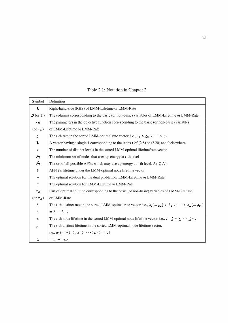
2.1 Notation in Chapter 2. . . . . . . . . . . . . . . . . . . . . . . . . . . . . . . . . . 21

2.2 Duality relationship between LMM node lifetime problem �� and LMM rate allo-

cation problem ��. . . . . . . . . . . . . . . . . . . . . . . . . . . . . . . . . . . 36

2.3 Locations (in meters) for each AFN in a ��-node network. . . . . . . . . . . . . . 38

2.4 Locations (in meters) for each AFN in a ��-node network. . . . . . . . . . . . . . 39

2.5 Node lifetime (in days) under the three approaches for the ��-node network. . . . . 39

2.6 Node lifetime (in days) under the three approaches for the ��-node network. . . . . 41

2.7 Numerical results verifying the duality relationship � � �� between the

LMM rate allocation problem �� and the LMM node lifetime problem �� for the

10-node network. . . . . . . . . . . . . . . . . . . . . . . . . . . . . . . . . . . . 45

2.8 Numerical results verifying the duality relationship � � �� between the

LMM rate allocation problem �� and the LMM node lifetime problem �� for the

20-node network. . . . . . . . . . . . . . . . . . . . . . . . . . . . . . . . . . . . 46


3.2 Each node’s location, data rate, and initial energy of the example sensor network. . 61

xv

3.3 Each node’s location, data rate and initial energy for a small ��-node network. . . . 66

3.4 Each node’s location, data rate and initial energy for a ��-node network. . . . . . . 68


4.2 Sensor locations, data rate, and initial energy of the example sensor network . . . . 92

4.3 Each node’s location, data rate, and initial energy for a small ��-node network. . . 95

4.4 �� -optimal result for the small ��-node network with � � ��. . . . . . . . . 97

4.5 Each node’s location, data rate, and initial energy for a ��-node network. . . . . . . 97

4.6 �� -optimal result for the ��-node network with � � ��. . . . . . . . . . . . 98




5.2 Available bands among all nodes in the network in the simulation study. . . . . . . 118

5.3 Simulation results for the first 40 data sets of ��-node networks. . . . . . . . . . . 120


6.2 Each node’s location and available frequency bands for the ��-node network. . . . 152

6.3 Source node, destination node, and rate requirement of the � sessions. . . . . . . . 152

xvi

Chapter 1

Introduction

1.1 Motivation and Objective

In recent years, there has been significant advances in wireless networking. Such advances are

fueled by the demand of new civil and military applications as well as advances in wireless com-

munication technology at the physical layer. These new advances at upper and lower layers have

brought many new research problems for networking researchers. Among these problems, a funda-

mental problem is to determine performance limits and to design a system to achieve these limits.

Due to new requirements (performance metrics) by these new applications and unique character-

istics (constraints) associated with these wireless networks, traditional analytical approaches are

no longer adequate. In this dissertation, we will develop several new approaches to study the

performance limits for wireless sensor networks and ad hoc networks.

Wireless ad hoc networks can be used to quickly build a network for peer-to-peer communi-

cation without first establishing a fixed infrastructure. Nodes in an ad hoc network are able to

organize themselves into a multi-hop network for wireless communications. Ad hoc networks can

be used where communication infrastructure is not available. On the other hand, wireless sensor

networks are dedicated to in-situ, unattended, and real-time surveillance and monitoring appli-

1

2

cations. Such network consists of battery-powered nodes that are endowed with a multitude of

sensing modalities [1]. Although there have been significant improvements in processor design

and computing, advances in battery technology still lag behind, making energy resource the funda-

mental challenge in wireless sensor networking. As a consequence of the energy constraint, a new

performance metric, namely, network lifetime, has become a vitally important performance metric

for wireless sensor networks.

Recent advances in physical layer technologies, e.g., ultra wideband (UWB), multiple-input

and multiple-output (MIMO), and cognitive radio (CR), have made profound impact on wireless

networks. In this dissertation, we consider CR, which is a revolution in radio technology. CR is

enabled by recent advances in RF design, signal processing, and communication software [83].

Fundamental characteristics of CR are that transmitted waveforms are defined by software and that

received waveforms are demodulated by software. This is in contrast to traditional hardware based

radios in which processing is done entirely in custom-made hardware circuitry. CR promises

unprecedented flexibility in radio communications and is viewed as an enabling technology for

dynamic spectrum access (DSA). For CR networks, we need to consider spectrum sharing among

CR nodes. A new metric, called bandwidth footprint product (BFP) is proposed to measure CR

nodes’ resource usage in both spectrum and space.

To explore the performance limits of these new wireless networks, it is necessary to consider

characteristics and constraints at multiple layers (i.e., power control at the physical layer, schedul-

ing at the link layer, and routing at the network layer). Such problems are typically very complex,

involving nonlinear, possibly non-convex relationship or constraints. As a result, developing the-

oretical results for these problems are very challenging and previous work are mostly heuristics

without any performance guarantee. In this dissertation, we will develop several efficient algo-

rithms to provide optimal or near-optimal solutions for these problems. These results are im-

portant not only for theoretical understanding, but also for providing guidelines to measure the

performance of any proposed distributed algorithm and protocol.

3

1.2 Summary of Contributions

In this dissertation, I will present solutions to a number of challenging problems in wireless sensor

networks and CR-based ad hoc networks.

1.2.1 Node Lifetime and Rate Allocation for Sensor Networks

We consider an overarching problem that encompasses both network lifetime (e.g., [17, 18]) and

network capacity (e.g., [56]). There have been active research efforts recently at the networking

layer on devising flow routing algorithms to maximize network lifetime [10, 11, 13, 17–19, 55,

115]. However, the network lifetime objective in most of these efforts has been centered around

maximizing the time until the first node fails. For wireless sensor networks that are primarily

designed for environmental monitoring or surveillance, the loss of a single node will only affect

the coverage of one particular area and will not affect the monitoring or surveillance capabilities of

the remaining nodes in the network. Consequently, it is important to investigate how to maximize

the lifetime for, not only the first node, but also all the nodes in the network. For fairness, we

maximize node lifetimes under the lexicographic max-min (LMM) criteria. Informally, the LMM

node lifetime problem attempts to maximize the time until a set of nodes drain up their energy

(which we call “drop point”) while minimizing the number of nodes that drain up their energy at

each drop point.

Recently, Brown et al. [15] studied the so-called “maximum node lifetime curve” problem,

which is equivalent to the LMM node lifetime problem. A key step in their solution procedure is

to use multiple independent linear programs (LPs) to determine the minimum set of nodes at each

drop point. We call this approach “serial LP with slack variable analysis” (SLP-SV). Although this

approach can solve the LMM node lifetime problem, its computational complexity is shown to be

exponential.

Motivated by Brown et al.’s work, we develop a polynomial-time algorithm to derive the LMM-

optimal node lifetime vector. We demonstrate that, for any given network configuration and initial

4

condition, our approach is always computationally more efficient than the slack variable (SV)

based approach in [15]. The computational effectiveness of our approach accrues from two impor-

tant techniques. First, we employ a link-based problem formulation, which significantly reduces

the problem size in comparison with a flow-based formulation in [15]. Second, we exploit the

so-called parametric analysis (PA) technique at each drop point to determine the minimum set of

nodes that use up their energy. PA is extremely simple and has a linear time complexity per node in

contrast to the SV-based approach in [15], which requires solving multiple additional LPs at each

drop point.

In addition to providing an efficient polynomial-time algorithm for the LMM-optimal node

lifetime vector computation, we also show how to obtain a corresponding flow routing solution

among the remaining active nodes at each stage, such that the LMM-optimal node lifetime vector

can indeed be achieved.

Another significant contribution in this work is that we extend our solution to the LMM node

lifetime problem to study the LMM rate allocation problem. In particular, we study the network

capacity (or rate allocation) problem under a given network lifetime requirement and the LMM

criterion. We show how to apply the PA technique to solve the LMM rate allocation problem.

Further, we show that there exists a simple and elegant duality relationship between the LMM

node lifetime problem and the LMM rate allocation problem. As a result, it is sufficient to solve

only one of these two problems. Important insights can be obtained by inferring duality results for

the other problem.

1.2.2 Base Station Placement for Sensor Networks

Network lifetime is highly dependent upon the physical topology of the wireless sensor network.

This is because energy expenditure at a node to transmit data to another node not only depends on

the data bit rate, but also on the physical distance between these two nodes. Consequently, it is

important to understand the impact of location related issues on network lifetime performance and

5

to optimize topology during network deployment stage.

We propose an approximation algorithm for base station placement problem to maximize the

network lifetime. The main idea in our approximation algorithm is to discretize cost parameters

(associated with energy consumption) with tight bounds under a given small error bound �. As a

result, we can divide the continuous search space into a finite number of subareas. By further ex-

ploiting the cost property of each subarea, we conceive a novel idea to represent each subarea with

a so-called “fictitious cost point” (FCP), which is a cost vector with each component representing

the upper bound of cost to a sensor node in the network. Based on these ideas, we have success-

fully reduced an infinite search space for base station location into a finite set of “points.” For each

point, we can apply an LP to find the corresponding achievable network lifetime and data routing

solution. By comparing the maximum achievable network lifetime among all the FCPs, we choose

the largest one and prove that locating the base station at any point in the subarea corresponding to

this best FCP is �� -optimal. We analyze the complexity of our approximation algorithm and

show that it is significantly lower than a state-of-the-art algorithm proposed in [32].

1.2.3 Mobile Base Station for Sensor Networks

The benefits of using mobile base station to prolong sensor network lifetime have been well recog-

nized [62, 110]. A mobile base station can alleviate the traffic aggregation burden from a fixed set

of sensor nodes near the base station to the rest of sensor nodes in the network, and it is possible

to extend the network lifetime significantly.

Although the potential benefit of using a mobile base station to prolong sensor network lifetime

is significant, the theoretical difficulty of this problem is tremendous. There are two components

that are tightly coupled in this problem. First, the location of the base station is now a function of

time. That is, at different time instances, we have a different physical network topology, with the

sink node being at different positions. Second, the traffic (or flow) routing behavior may change

with both time as well as the location of the base station. As a result, to maximize the network

6

lifetime, we need to consider both base station movement and time-dependent flow routing.

We offer an in-depth study on network lifetime performance when a mobile base station is

employed. As a first step, we show that as far as network lifetime objective is concerned, flow

routing only needs to be dependent on the base station location, regardless of when the base station

is present at this location. Further, the specific time instances for the base station to visit a location

is not important, as long as the total sojourn time for the base station to be present at this location

is fixed. With this finding, we make a novel transformation from a time-dependent problem formu-

lation to location (space)-dependent problem formulation. As a second step, we show that when

base station is only allowed to be present at a finite set of pre-determined points (called constrained

mobile base station (C-MB) problem), we can find the optimal time duration for the base station

to stay on each of these points (as well as the corresponding flow routing solution) via a single LP.

Building upon these results, we show that for the un-constrained mobile base station (U-MB)

problem, i.e., the base station can be present at any point in the two dimensional plane, we can

develop a polynomial-time approximation algorithm to provides a ��-optimal solution, where �

can be made arbitrarily small depending on required precision. The main idea in this approximation

algorithm is again to divide the search space into subareas and to represent each subarea by an FCP.

As a result, we can apply the LP approach developed for the C-MB problem on these FCPs and

develop provably ��-optimal solution. This is the first theoretical result on mobile base station

problem.

1.2.4 Optimal Spectrum Sharing for CR Networks

A cognitive radio (CR) is a frequency-agile data communication device with a rich control and

monitoring (spectrum sensing) interface. It capitalizes advances in signal processing and radio

technology, as well as recent advancements in spectrum policy [69, 83]. A frequency-agile radio

module is capable of reconfiguring RF and switching to newly-selected frequency bands. Thus, a

CR can be programmed to tune to and operate on specific frequency bands over a wide range of

7

spectrum [83].

We focus on the multi-hop networking problem for a CR-based wireless ad hoc network. In

such a network, each node has a set of spectrum bands that it can use. Due to the unequal size of

spectrum bands, it may be necessary to further divide each band into sub-bands for transmission

and reception. Suppose there are a set of user sessions in the network that is characterized by a

set of source-destination pairs each having certain rate requirement. We consider how to perform

spectrum allocation, scheduling and interference avoidance, and multi-hop multi-path routing such

that the required network-wide radio spectrum resource is minimized.

There are two reasons that we propose to investigate this problem. First, the cross-layer con-

straints that we will present is general and characterize common agreed behaviors of packet radio

networks. Therefore, the solution procedure can be easily modified to address other performance

objectives (e.g., rates or capacity). Second, it has been shown in [61] that so-called space band-

width product is an extremely useful performance metric in the context of multi-hop CR networks.

In the absence of power control, this metric degenerates into our performance objective.

To formulate the problem mathematically, we characterize the behavior and constraints from

multiple layers for a general multi-hop CR network. Special attention is given to modeling of

spectrum sharing and (unequal size) sub-band division, scheduling and interference modeling, and

multi-path routing. We formulate an optimization problem with the objective of minimizing the

required network-wide radio spectrum resource for a set of source-destination pair rate require-

ments. Since such a problem formulation is a mixed integer nonlinear program, which is NP-hard

in general [40], we aim to develop a near-optimal solution. We first develop a lower bound by us-

ing a linear relaxation. This lower bound can be used as a measure for the quality of any solution.

The proposed algorithm is based on a novel sequential fixing (SF) procedure where the determina-

tion of integer variables is performed iteratively through a sequence of LPs. Upon completing the

fixing of the integer variables, the value of the other variables in the optimization problem can be

obtained by solving an LP. Simulations show that the results obtained by the SF algorithm are very

close to the lower bound, thus suggesting that the solutions obtained by the SF algorithm are even

8

closer to the optimum and thus near-optimal.

1.2.5 Optimal Power Control for CR Networks

We further consider how to support a set of user communication sessions (each with a rate require-

ment) by jointly optimizing power control, scheduling, and routing such that the required radio

resource and interference area in the network are minimized. We follow the so-called “protocol

model” [44] for interference modeling. Since power control directly affects the signal power at the

receiving node and the interference power at other nodes, we find that it has profound impact on

scheduling feasibility, bandwidth efficiency, and problem complexity.

We develop a formal mathematical model for scheduling when power control is employed.

Along the line of protocol interference modeling, we develop a formal mathematical model for

power control and scheduling. This model extends existing deterministic interference model and

can be used for a range of problems where power control is part of the optimization space.

Based on this model, we formulate a joint power control, scheduling, and routing problem to

support a set of user communication sessions with the objective of minimizing radio resource re-

quirement and interference area. Subsequently, we develop an efficient solution procedure based

on the branch-and-bound framework and convex hull relaxations to solve this cross-layer optimiza-

tion problem. The solution obtained via our approach yields a �� -optimal solution, where �

is a small positive constant reflecting our desired accuracy in the final solution. By applying the

solution procedure on sample random networks, we demonstrate quantitatively that power control

has significant impact on scheduling feasibility, bandwidth efficiency, and BFP.

1.3 Dissertation Outline

The remainder of this dissertation is organized as follows. Chapter 2 presents efficient serial LP

algorithm based on parametric analysis (SLP-PA) for the LMM node lifetime problem and the

9

Table 1.1: General notation.

Symbol Definition Symbol Definition

� The search space for the base station � The set of nodes in the network

�� The �-th subarea in the search space �� The center of �

� The base station in a sensor network �� Data rate at node �

�� Distance from node � to node � �� Data rate of session �

�� Destination node of session � � The radius of �

� Initial energy at node � �� Source node of session �

�� Data rate from on link �� Network lifetime

�� Data rate that is attributed to session � � �� The set of nodes that can use band �

on link �� to transmit to node �

�� Propagation gain from node � to node � ��

� �� , the set of nodes that can

�� Number of circles at sensor node � transmit to node �

under a given � �� The total bit volume from node � to �

�� The set of nodes that can use band � � Path loss index

and make non-neglectable interference �rec Power consumption coefficient

at node � for receiving data

� The set of active sessions in the network �� Constant terms in power consumption

� The number of pre-determined locations coefficient for transmitting data

or the number of subareas �� Coefficient of power consumption

�� The set of available bands at a cognitive for transmitting data from node � to �

radio (CR) node � �min�� max

�� Lower and upper bounds of ��

� �� , the set of available bands �� , the transmission cost

in a CR network for the �-th circle

��

�� , the set of available bands � Desired small error bound, � � �

for link �� Ambient Gaussian noise density

� The number of nodes in the network �� A �� -optimal solution

10

LMM rate allocation problem. We also show the duality relationship between these two problems.

In Chapter 3, we present an approximation algorithm based on fictitious cost point (FCP) for the

base station placement problem such that the network lifetime is at least �� of the optimum.

Chapter 4 presents an approximation algorithm for the mobile base station problem that provides

a �� -optimal network lifetime. In Chapter 5, we present a sequential fixing (SF) algorithm

for a multi-hop CR network to minimize the total required spectrum for a given set of communi-

cation sessions. In Chapter 6, we first develop a detailed mathematical model for power control,

scheduling, and routing. Then, we develop a branch-and-bound solution procedure to minimize

network-wide BFP for the given set of communication sessions. Table 1.1 lists the general nota-

tion used in this dissertation.

Chapter 2

Node Lifetime and Rate Allocation

Problems for Wireless Sensor Networks

2.1 Introduction

Wireless sensor networks [1] consist of battery-powered nodes that are endowed with a multitude

of sensing modalities including multimedia (e.g., video, audio) and scalar data (e.g., temperature,

pressure, light, magnetometer, infrared). The demand for sensor networks is spurred by numerous

applications that require in-situ, unattended, high-precision, and real-time observations over a vast

area. Although there have been significant improvements in processor design and computing, ad-

vances in battery technology still lag behind, making energy resource the fundamental challenge in

wireless sensor networking. Consequently, there have been active research efforts on performance

limits of wireless sensor networks. These performance limits include, among others, network life-

time (e.g., [17,18]) and network capacity (e.g., [56]). Network lifetime refers to the maximum time

limit that nodes in the network remain alive until one or more nodes drain up their energy, while

network capacity typically refers to the maximum amount of bit volume that can be successfully

delivered to the base station (“sink node”) by all the nodes in the network.

11

12

In this chapter, we consider an overarching problem that encompasses both performance met-

rics. There have been active research efforts recently at the networking layer on devising flow

routing algorithms to maximize network lifetime [10, 11, 13, 17–19, 55, 115]. However, the net-

work lifetime objective in most of these efforts has been centered around maximizing the time

until the first node fails. Although the time until the first node fails is an important measure from

the complete network coverage point of view, this performance metric alone cannot measure the

lifetime performance behavior for all nodes in the network. For wireless sensor networks that are

primarily designed for environmental monitoring or surveillance, the loss of a single node will

only affect the coverage of one particular area and will not affect the monitoring or surveillance

capabilities of the remaining nodes in the network. This is because the remaining nodes in the

network can adjust their transmission power (via power control) and reconfigure themselves into

a new network routing (relay) topology so that information collected at the remaining nodes can

still be delivered successfully to the base station. Consequently, it is important to investigate how

to maximize the lifetime for, not only the first node, but also all the other nodes in the network.

For fairness, we maximize node lifetimes under the lexicographic max-min (LMM) criteria, which

will be formally defined in Section 2.2.3. We call this the LMM node lifetime problem.

Recently, Brown et al. [15] studied this problem under the so-called “maximum node lifetime

curve” problem, which is equivalent to the LMM node lifetime problem. Informally, the maximum

node life curve attempts to maximize the time until a set of nodes drain up their energy (which we

call the drop point) while minimizing the number of nodes that drain up their energy at each drop

point. The main contribution by Brown et al. [15] is the development of a procedure to solve the

maximum node lifetime curve problem. A key step in their procedure is to use multiple indepen-

dent linear programming (LP) calculations to determine the minimum set of nodes at each drop

point, which we call “serial LP with slack variable analysis” (SLP-SV). Although this approach can

solve the LMM node lifetime problem, its computational complexity is shown to be exponential,

which could be a potential problem for large-scale networks.

Inspired by Brown et al.’s work on the LMM node lifetime problem, in this chapter, we de-

velop a polynomial-time algorithm to derive the LMM-optimal node lifetime vector. In addition,

13

we demonstrate that, for any given network configuration and initial condition, our approach is

always significantly computationally more efficient than the slack variable (SV) based approach

in [15]. Consequently, this leads to an even stronger performance guarantee than the commonly

used worst case complexity criteria. The computational effectiveness of our approach accrues from

two important techniques. First, we employ a link-based problem formulation, which significantly

reduces the problem size in comparison with a flow-based formulation used in [15]. Second, which

is also the most significant contribution in this chapter, we exploit the so-called parametric analysis

(PA) technique at each drop point to determine the minimum set of nodes that use up their energy.

We show that this technique is a powerful tool in determining the minimum node set for each drop

point. When the problem is non-degenerate, it is extremely simple and has a linear time complexity

per node in contrast with the SV-based approach proposed in [15], which requires solving multiple

additional LPs at each drop point. Even for the rare case, when the problem is degenerate, using

the PA technique still is more efficient than the SV-based approach as it decreases the number of

additional LPs that need to be solved at each drop point.

In addition to providing an efficient polynomial-time algorithm for the LMM-optimal node

lifetime vector computation, we also develop a simple polynomial-time algorithm that provides a

corresponding flow routing solution among the remaining alive nodes at each stage such that the

LMM-optimal node lifetime vector can indeed be achieved. A nice property about this algorithm

is that it can be executed in parallel (instead of in serial) for all the stages.

We also extend the PA technique for the LMM node lifetime problem to address the LMM

rate allocation problem. In particular, we study the network capacity (or rate allocation) problem

under a given network lifetime requirement. Again, for fairness, we use of the LMM criterion in

rate allocation. In addition to solve the LMM rate allocation problem, we show that there exists a

simple and elegant duality relationship between the LMM node lifetime problem and the LMM rate

allocation problem. As a result, it is sufficient to solve only one of these two problems. Important

insights can be obtained by inferring duality results for the other problem.

The remainder of this chapter is organized as follows. In Section 2.2, we describe the system

14

model and problem statement for this research, including the reference network architecture, nodal

power dissipation behavior, and the LMM node lifetime problem description. We also describe

a naive approach to address this problem and discuss why it usually gives an incorrect solution.

Section 2.3 presents the link-based LMM problem formulation and our efficient serial LP algo-

rithm based on parametric analysis, which we call SLP-PA. We also analyze the complexity of

our algorithm and compares it with that in [15]. In Section 2.4, we introduce the LMM rate al-

location problem and apply the SLP-PA algorithm to solve it. Section 2.5 shows an interesting

duality relationship between the LMM node lifetime problem and the LMM rate allocation prob-

lem. Numerical results using the SLP-PA approach, the corresponding flow routing solution, and

the duality relationship are given in Section 2.6. Section 2.7 reviews related work and Section 2.8

concludes this chapter.

2.2 System Modeling and Problem Formulation

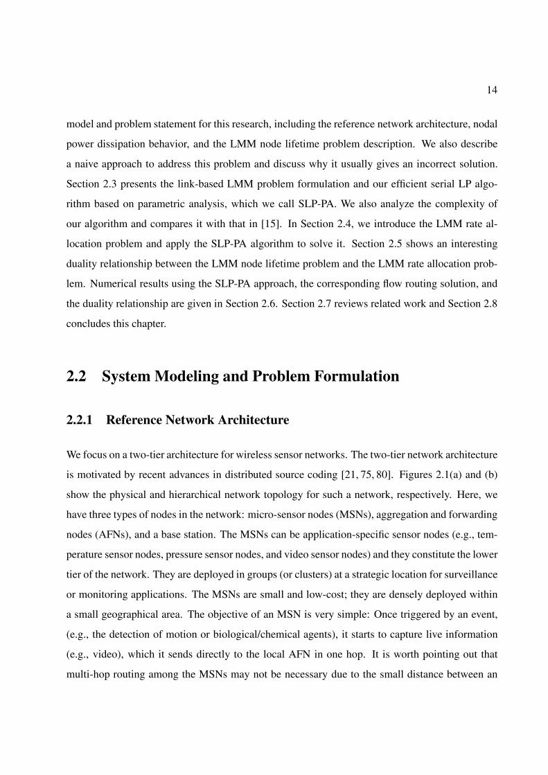
2.2.1 Reference Network Architecture

We focus on a two-tier architecture for wireless sensor networks. The two-tier network architecture

is motivated by recent advances in distributed source coding [21, 75, 80]. Figures 2.1(a) and (b)

show the physical and hierarchical network topology for such a network, respectively. Here, we

have three types of nodes in the network: micro-sensor nodes (MSNs), aggregation and forwarding

nodes (AFNs), and a base station. The MSNs can be application-specific sensor nodes (e.g., tem-

perature sensor nodes, pressure sensor nodes, and video sensor nodes) and they constitute the lower

tier of the network. They are deployed in groups (or clusters) at a strategic location for surveillance

or monitoring applications. The MSNs are small and low-cost; they are densely deployed within

a small geographical area. The objective of an MSN is very simple: Once triggered by an event,

(e.g., the detection of motion or biological/chemical agents), it starts to capture live information

(e.g., video), which it sends directly to the local AFN in one hop. It is worth pointing out that

multi-hop routing among the MSNs may not be necessary due to the small distance between an

15

Base Station

Aggregation and Forwarding Node(AFN) Micro−Sensor Node

(MSN)

(a) Physical network topology.

Lower tier

Upper tier

Base Station

AFN

MSN

(b) An instance of routing topology among AFNs.

Figure 2.1: Reference architecture for a two-tier wireless sensor network.

16

MSN and its AFN. By deploying these inexpensive MSNs in clusters, and within proximity of a

strategic location, it is possible to obtain a comprehensive view of the area situation by exploring

the correlation among the scenes collected at each MSN [21]. Furthermore, the reliability of area

surveillance capability can also be improved through redundancy among the MSNs in the same

cluster.

For each cluster of MSNs, there is one AFN, which is different from an MSN in terms of both

its physical properties and functions. The primary functions of an AFN are: (1) data aggregation

(or “fusion”) for information flows coming from the local cluster of MSNs, and (2) forwarding

(or relaying) the aggregated information to the next hop AFN toward the base station. For data

fusion, an AFN analyzes the content of each data stream (e.g., video) it receives, from which it

composes a complete scene by exploiting the correlation among each individual data stream from

the MSNs. An AFN also serves as a relay node for other AFNs to carry traffic toward the base

station. Although an AFN is expected to be provisioned with much more energy than an MSN,

it also consumes energy at a substantially higher rate (due to wireless communication over large

distances). Consequently, an AFN has limited lifetime. Upon the depletion of energy at an AFN,

we expect that the coverage for the particular area under surveillance will be lost, despite the fact

that some of the MSNs within the cluster may still have remaining energy.1

The third component in the two-tier architecture is the base station. The base station is, es-

sentially, the sink node for all the AFNs in the network. A base station may be assumed to have

a sufficient battery resource provision, or its battery may be re-provisioned during its course of

operation. Therefore, its power dissipation is not a concern in our investigation.

In summary, the main functions of the lower tier MSNs are data acquisition and compression

while the upper-tier AFNs are used for data fusion and relaying the information to the base station.

The routing topology can be controlled by the power level of a node’s transmitter [43,78,86,105],

which in turn controls the distance coverage of an AFN. Consequently, by adjusting the power

level of an AFN’s transmitter, we can form different network routing topologies.

1We assume that each MSN can only forward information to its local AFN for processing (e.g., video fusion).

17

2.2.2 Energy Model

For an AFN, the power consumption by data communication (i.e., receiving and transmitting) is

the dominant factor [1]. The power dissipation at the transmitter can be modeled as:

t�� (2.1)

where t�� is the power dissipated at node when it is transmitting to node �, �� is the bit rate

transmitted from node to node �, and �� is the power consumption cost of radio link � � and

is given by

�� (2.2)

where � and � are two constant terms, �� is the distance between these two nodes, and � is the

path loss index, with � � � � � [82]. The power dissipation at a receiver can be modeled as [82]:

r� � rec �

��

�� (2.3)

where rec is a constant.

The above transmission and reception energy model assumes a contention-free MAC protocol,

where interference from simultaneous transmissions can be effectively avoided. For deterministic

rate traffic pattern model in this chapter, a contention-free MAC protocol is fairly easy to design

(e.g., [93]) and its discussion is beyond the scope of this chapter.

2.2.3 The Lexicographic Max-Min Node Lifetime Problem

For a network having a set � of AFNs, suppose that AFN � generates data stream at a rate

��, and that the initial energy at this node is given by ��. For an AFN, the power consumption

by data communication (i.e., receiving and transmitting) is the dominant factor [1]. Then, it is

straightforward to use a linear programming (LP) approach to find an optimal routing solution

18

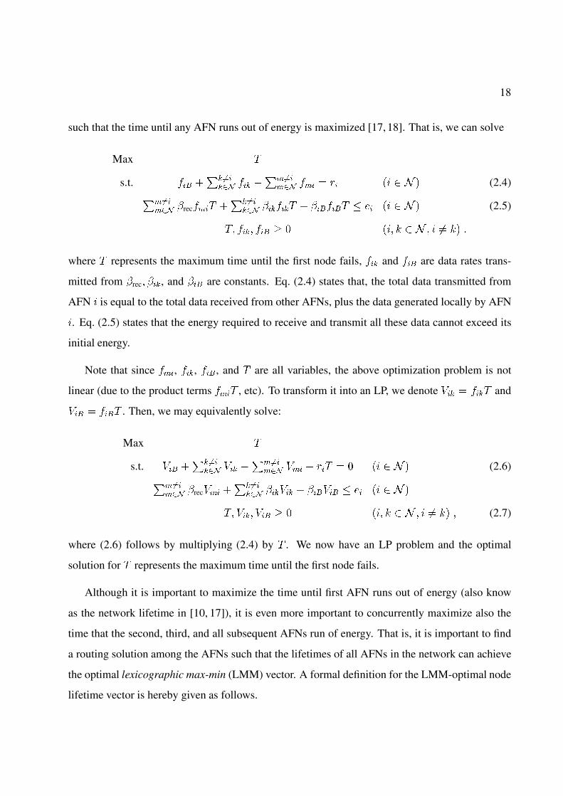
such that the time until any AFN runs out of energy is maximized [17, 18]. That is, we can solve

Max �

s.t. ��

��

�� (2.4)�� rec��

�� (2.5)

��

where � represents the maximum time until the first node fails, �� and �� are data rates trans-

mitted from rec� ��, and �� are constants. Eq. (2.4) states that, the total data transmitted from

AFN is equal to the total data received from other AFNs, plus the data generated locally by AFN

. Eq. (2.5) states that the energy required to receive and transmit all these data cannot exceed its

initial energy.

Note that since ��, ��, �� , and � are all variables, the above optimization problem is not

linear (due to the product terms �� , etc). To transform it into an LP, we denote �� and

�� . Then, we may equivalently solve:

Max �

s.t. ��

��

�� (2.6)�� rec��

��

�� (2.7)

where (2.6) follows by multiplying (2.4) by � . We now have an LP problem and the optimal

solution for � represents the maximum time until the first node fails.

Although it is important to maximize the time until first AFN runs out of energy (also know

as the network lifetime in [10, 17]), it is even more important to concurrently maximize also the

time that the second, third, and all subsequent AFNs run of energy. That is, it is important to find

a routing solution among the AFNs such that the lifetimes of all AFNs in the network can achieve

the optimal lexicographic max-min (LMM) vector. A formal definition for the LMM-optimal node

lifetime vector is hereby given as follows.

19

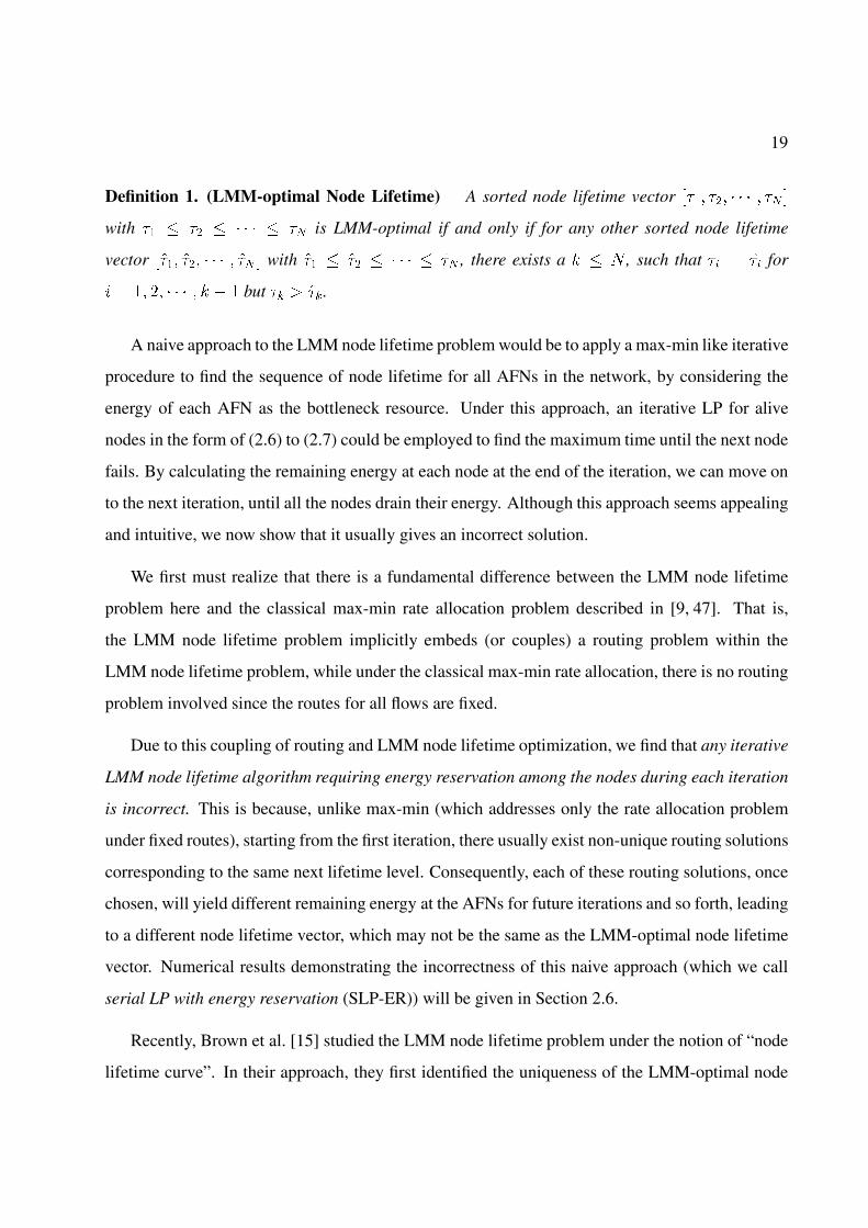
Definition 1. (LMM-optimal Node Lifetime) A sorted node lifetime vector ��

with �� is LMM-optimal if and only if for any other sorted node lifetime

vector �� with �� , there exists a � � � , such that �� for

� �� but �� .

A naive approach to the LMM node lifetime problem would be to apply a max-min like iterative

procedure to find the sequence of node lifetime for all AFNs in the network, by considering the

energy of each AFN as the bottleneck resource. Under this approach, an iterative LP for alive

nodes in the form of (2.6) to (2.7) could be employed to find the maximum time until the next node

fails. By calculating the remaining energy at each node at the end of the iteration, we can move on

to the next iteration, until all the nodes drain their energy. Although this approach seems appealing

and intuitive, we now show that it usually gives an incorrect solution.

We first must realize that there is a fundamental difference between the LMM node lifetime

problem here and the classical max-min rate allocation problem described in [9, 47]. That is,

the LMM node lifetime problem implicitly embeds (or couples) a routing problem within the

LMM node lifetime problem, while under the classical max-min rate allocation, there is no routing

problem involved since the routes for all flows are fixed.

Due to this coupling of routing and LMM node lifetime optimization, we find that any iterative

LMM node lifetime algorithm requiring energy reservation among the nodes during each iteration

is incorrect. This is because, unlike max-min (which addresses only the rate allocation problem

under fixed routes), starting from the first iteration, there usually exist non-unique routing solutions

corresponding to the same next lifetime level. Consequently, each of these routing solutions, once

chosen, will yield different remaining energy at the AFNs for future iterations and so forth, leading

to a different node lifetime vector, which may not be the same as the LMM-optimal node lifetime

vector. Numerical results demonstrating the incorrectness of this naive approach (which we call

serial LP with energy reservation (SLP-ER)) will be given in Section 2.6.

Recently, Brown et al. [15] studied the LMM node lifetime problem under the notion of “node

lifetime curve”. In their approach, they first identified the uniqueness of the LMM-optimal node

20

lifetime vector. Based on this property, they developed an iterative procedure to solve the LMM

node lifetime problem. In particular, they developed a revised simplex method to calculate the

maximum node lifetime curve (equivalent to the LMM-optimal node lifetime vector). A key step

in their procedure is to use multiple independent LPs to maximize the sum of slack variables in

order to determine the minimum node set at each lifetime level. During each iteration, only the

lifetime level and the corresponding minimum set of nodes are determined, and there is no resource

reservation process among the nodes. Although their proposed approach solves the LMM node

lifetime problem, there still remain significant issues to be addressed. Among others, the problem

formulation proposed in [15] is shown to be of exponential computational complexity, which could

become problematic when the scale of the network becomes large.

2.3 An Efficient Algorithm Based on Parametric Analysis

In this section, we present an efficient algorithm for the LMM node lifetime problem. Unlike

the serial LP with slack variable analysis (SLP-SV) approach in [15], our approach results in a

polynomial running time. Moreover, for any given network configuration and initial condition, our

approach is much simpler than the slack variable (SV) based approach in [15]. The computational

effectiveness of our approach hinges upon two important techniques. First, we employ a link-based

problem formulation that significantly reduces the problem size in comparison with a flow-based

formulation adopted in [15]. Second, we invoke a parametric analysis (PA) procedure at each

stage to determine the minimum node set at each lifetime level. For non-degenerate problems,

this parametric analysis results in only a linear time computational complexity per node, while

the SV-based approach in [15] requires the solution of multiple independent LPs to determine the

minimum set of nodes at each lifetime level. Even for the rare case when the problem is degenerate,

using our parametric analysis technique is still more efficient than the SV-based approach because

it decreases the number of additional LPs that needs to be solved at each lifetime level. In the

remainder of this section, we elaborate on the details of our serial LP algorithm based on parametric

analysis (SLP-PA). Table 2.1 shows the notation that are used only in this chapter.

21

Table 2.1: Notation in Chapter 2.

Symbol Definition

� Right-hand-side (RHS) of LMM-Lifetime or LMM-Rate

(or ) The columns corresponding to the basic (or non-basic) variables of LMM-Lifetime or LMM-Rate

�� The parameters in the objective function corresponding to the basic (or non-basic) variables

(or �� ) of LMM-Lifetime or LMM-Rate

�� The �-th rate in the sorted LMM-optimal rate vector, i.e., ��

�� A vector having a single 1 corresponding to the index � of (2.8) or (2.20) and 0 elsewhere

� The number of distinct levels in the sorted LMM-optimal lifetime/rate vector

�� The minimum set of nodes that uses up energy at �-th level

�� The set of all possible AFNs which may use up energy at �-th level, ��

�� AFN �’s lifetime under the LMM-optimal node lifetime vector

� The optimal solution for the dual problem of LMM-Lifetime or LMM-Rate

� The optimal solution for LMM-Lifetime or LMM-Rate

�� Part of optimal solution corresponding to the basic (or non-basic) variables of LMM-Lifetime

(or �� ) or LMM-Rate

�� The �-th distinct rate in the sorted LMM-optimal rate vector, i.e., ��

Æ� � ��

� The �-th node lifetime in the sorted LMM-optimal node lifetime vector, i.e., � � � � � � � � �

!� The �-th distinct lifetime in the sorted LMM-optimal node lifetime vector,

i.e., !�� !� � � � � � !��

"� � !� � !��

22

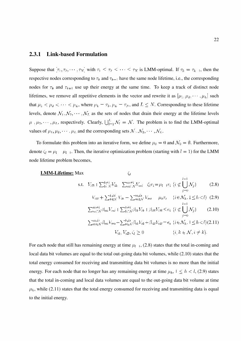
2.3.1 Link-based Formulation

Suppose that �� with �� is LMM-optimal. If �� , then the

respective nodes corresponding to �� and �� have the same node lifetime, i.e., the corresponding

nodes for �� and �� use up their energy at the same time. To keep a track of distinct node

lifetimes, we remove all repetitive elements in the vector and rewrite it as �� such

that �� , where �� , �� , and � � � . Corresponding to these lifetime

levels, denote �� as the sets of nodes that drain their energy at the lifetime levels

�� , respectively. Clearly,��

�� . The problem is to find the LMM-optimal

values of �� and the corresponding sets �� .

To formulate this problem into an iterative form, we define �� and �� . Furthermore,

denote � � � � ��. Then, the iterative optimization problem (starting with � � �) for the LMM

node lifetime problem becomes,

LMM-Lifetime: Max �

s.t. ��

��

��

�� (2.8)

��

��

�� (2.9)

��rec��

��

��

�� (2.10)

��rec��

�� (2.11)

��

For each node that still has remaining energy at time ��, (2.8) states that the total in-coming and

local data bit volumes are equal to the total out-going data bit volumes, while (2.10) states that the

total energy consumed for receiving and transmitting data bit volumes is no more than the initial

energy. For each node that no longer has any remaining energy at time ��, � � � � �, (2.9) states

that the total in-coming and local data volumes are equal to the out-going data bit volume at time

��, while (2.11) states that the total energy consumed for receiving and transmitting data is equal

to the initial energy.

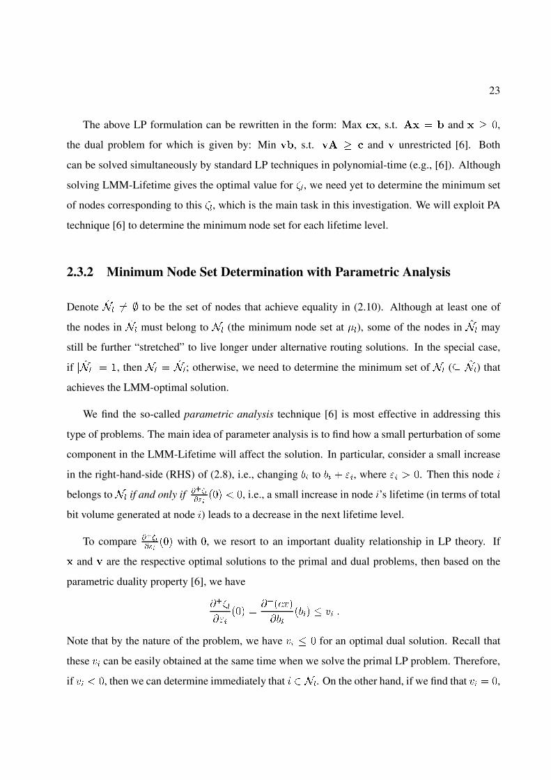
23

The above LP formulation can be rewritten in the form: Max ��, s.t. �� and � �,

the dual problem for which is given by: Min ��, s.t. �� and � unrestricted [6]. Both

can be solved simultaneously by standard LP techniques in polynomial-time (e.g., [6]). Although

solving LMM-Lifetime gives the optimal value for �, we need yet to determine the minimum set

of nodes corresponding to this �, which is the main task in this investigation. We will exploit PA

technique [6] to determine the minimum node set for each lifetime level.

2.3.2 Minimum Node Set Determination with Parametric Analysis

Denote �� to be the set of nodes that achieve equality in (2.10). Although at least one of

the nodes in �� must belong to � (the minimum node set at �), some of the nodes in �� may

still be further “stretched” to live longer under alternative routing solutions. In the special case,

if �� , then � � ��; otherwise, we need to determine the minimum set of � (� ��) that

achieves the LMM-optimal solution.

We find the so-called parametric analysis technique [6] is most effective in addressing this

type of problems. The main idea of parameter analysis is to find how a small perturbation of some

component in the LMM-Lifetime will affect the solution. In particular, consider a small increase

in the right-hand-side (RHS) of (2.8), i.e., changing �� to �� , where �� . Then this node

belongs to� if and only if ��

�� , i.e., a small increase in node ’s lifetime (in terms of total

bit volume generated at node ) leads to a decrease in the next lifetime level.

To compare ��

�� with �, we resort to an important duality relationship in LP theory. If

� and � are the respective optimal solutions to the primal and dual problems, then based on the

parametric duality property [6], we have

��

��

��

Note that by the nature of the problem, we have �� for an optimal dual solution. Recall that

these �� can be easily obtained at the same time when we solve the primal LP problem. Therefore,

if �� , then we can determine immediately that �. On the other hand, if we find that �� ,

24

it is not clear whether ��

�� is strictly negative or � and further analysis is thus needed.

For each node with �� , we must perform a complete PA to see whether this RHS can be

further increased without changing the objective value of LMM-Lifetime. If there is no change,

then we can determine that node � �; otherwise, �.

Assume that the optimal solution is ��, where �� and �� denote the set of basic and non-

basic variables; � and � denote the columns corresponding to the basic and non-basic variables;

�� and �� denote the objective function coefficient vectors for the basic and non-basic variables;

and denotes the objective value. Then the corresponding canonical equations yield [6]

� ��

��

��

If � is replaced by � � ��, where the column vector �� has a single � corresponding to node in

the set of constraints (2.8) and has � elements otherwise, then the only change in the constraints

due to this perturbation is that �� will be replaced by ��. Consequently, the objective

value for the current basis becomes �� . Furthermore, as long as �� is

nonnegative, the current basis remains optimal. Denote � � �� and �� and let �� be

an upper bound for �� such that the current basis remains optimal, we have

��

�

��

� �� (2.12)

If �� , the optimal objective value varies according to �� for � � �� . Since

� � �� and �� , we have ��

�� . Thus, the objective value will not change

for �� , and consequently, the lifetime for node can be “stretched” to last longer beyond

current lifetime level �. That is, node does not belong to the minimum node set �.

For most practical problems, this directly yields whether � or � � for all ��. But in

the rare event where �� , the problem is degenerate. To develop a polynomial-time algorithm,

denote � as the set of all nodes with �� and � the set of all nodes with �� and �� .

25

Then we solve the following LP to maximize the slack variables for nodes in �.

MSV: Max�

��

s.t. ��

��

��

��

��

��

��

��

��

��

��

�� rec��

��

��

��

��

�� rec��

��

��

��

��

��

If the optimal objective value is �, then no node in � can have a positive ��, i.e., these nodes should

all belong to �. That is, these nodes should all belong to � and we have � � � � �. On the

other hand, if the optimal objective value is positive, then some nodes in � must have positive ��,

i.e., these nodes should not belong to �. Consequently, we remove these nodes from � and if

� �� , we solve another MSV. This procedure will terminate when the optimal objective value is

� or � � �.

In a nutshell, the complete PA procedure for the determination of whether or not a node ��

belongs to the minimum node set � can be summarized as follows.

Algorithm 1. (Minimum Node Set Determination with PA)

1. Initialize � � � and � � �.

2. For each node ��,

(a) if �� , add node to �;

(b) otherwise, using �� (which is readily available after solving an LMM-Lifetime), com-

pute � � ��, �� , and �� according to (2.12). If �� , add to �.

26

3. If � � �, let� � � and stop, else build and solve an MSV.

4. If the optimal objective value is �, let � � � � � and stop. Otherwise, remove all nodes

with �� from � and go to Step 3.

The following lemma establishes an important property for the minimum node set obtained at

each lifetime level.

Lemma 1. Under the LMM-optimal solution, the set of nodes in the minimum node set at each

lifetime level is unique.

Proof. By the definition of LMM-optimal node lifetime vector (Definition 1), the optimal node

lifetimes (� values) are unique and the corresponding number of nodes in the minimum node set

( � values) are also unique. To show that the group of physical nodes in each � is also unique,

we employ the parametric simplex approach to determine the minimum node set as follows.

In essence, the parametric simplex approach solely relies on PA technique without resorting

the SV approach even when the problem is degenerate. That is, when the problem is degenerate,

i.e., for some node ��, we have �� and �� , then the basis can change while the optimal

objective value remains unchanged. We can analyze �� and �� under the new basis to determine

whether or not node belongs to the minimum node set �. If we still have �� and �� ,

the basis can change again with the same optimal objective value. To prevent cycling back to a

previous basis, we can use a de-cycling rule [6]. Thus, this procedure is guaranteed to terminate

within a finite number of steps and we can determine whether or not node indeed belongs to the

minimum node set �.

Note that in the above parametric simplex approach, the set of physical nodes corresponding to

� is uniquely determined since the analysis is conducted independently for each node. Therefore,

upon the completion of all stages, the group of physical nodes in each minimum node set is unique.

27

2.3.3 LMM-Optimal Routing Solution

Non-uniqueness of Routing Solution. The solution to the LMM node lifetime problem would

not be complete without a corresponding routing solution. The first question to ask is whether

such a routing solution is unique. We show that, although the set of physical nodes corresponding

to the minimum node set at each stage is unique (Lemma 1), the routing solution is non-unique.

This is because upon the completion of the last LMM-Lifetime in SLP-PA, there usually exist non-

unique bit volume solutions (�� and �� values along each radio link), all of which can achieve

the same unique objective values (�� values). As the bit volumes (�� and �� values) along each

radio link are non-unique, the corresponding routing solution is, as a result, also non-unique. This

observation is formally stated in the following lemma.

Lemma 2. The routing solution corresponding to the LMM-optimal node lifetime vector can be

non-unique.

Incidentally, this result corrects an error in [15] (Lemma 3.2), which incorrectly states that such

a routing solution is unique.

An Optimal Routing Solution. Given that the optimal routing solution is non-unique, there are

potentially many possible routing solutions that achieve the LMM-optimal node lifetime vector. In

this section, we present a simple approach that provides an LMM-optimal routing solution.

The main task in this algorithm is to define flows from the bit volumes (�� and �� values),

which are obtained upon the completion of the last LMM-Lifetime in our SLP-PA approach. Note

that the bit volumes obtained here represent the total amount of bit volume being transported be-

tween the nodes during �� , where �� is the time that the last set of nodes drain their

energy. The main result here is that if we let the total amount of out-going flow at a node be dis-

tributed proportionally to the bit volumes on each out-going link for all the remaining alive nodes

at each stage, then we can achieve the drop points �� as well as the corresponding

minimum node sets �� . The algorithm is formally described as follows.

28

Algorithm 2. (An Optimal Flow Routing Solution) Upon the completion of the SLP-PA algo-

rithm for the LMM node lifetime vector, we have the drop points (in strictly increasing order)

�� , the corresponding minimum physical node sets �� , and the total

amount of bit volume on each radio link (i.e., �� and ��). The following algorithm gives an

LMM-optimal flow routing solution for the corresponding time interval �� , where ��

and � � �� .

1. Denote � � � ��

��, with �� . Initialize all flows to zero, i.e., � �� , � ��

��

for � � � � �� .

2. If � � �, then stop, else choose a node from � such that2

� either node does not receive data from any other node, or

� all nodes from which node receives data are not in �.

3. The flow routing at node during �� is then defined as

��

��

��

��

��

��

��

� ��

��

��

��

��

� ��

�

where the �� values, if not zero, have all been defined before calculating the flow routing

for node .

4. Let � � � � � � and go to Step 2.

As shown in this algorithm, for each time interval �� , � � �� , we initialize

� as the set of remaining alive nodes at this stage, which is represented by � � � ��

��.

For these nodes, we compute a flow routing by starting with the “boundary” nodes and then move

2Such a node must exist when �� , since there is no cycle in an LMM-optimal solution, i.e., we do nothave �� . Otherwise, by reducing these volumes a little further, we can increase thecorresponding nodes’ lifetimes.

29

to the “interior” nodes. More precisely, we will calculate the flow routing for a node if and only

if we have calculated the flow routing for each node ! that has traffic coming into node . The

out-going flow at node is calculated by distributing the aggregated in-coming flow proportionally

according to the overall bit volume along its out-going radio links. As an example, suppose that

during �� , node � receives an aggregated flow of rate � kb/s and generates �� kb/s amount of

data locally. Assume that �� kb, �� kb, and �� kb over �� . Then the

out-going flow at node � is routed as follows: � �� kb/s, � ��

� � �� kb/s, and �� kb/s.

We now give a formal proof that the flow routing solution defined by Algorithm 2 will indeed

give the LMM-optimal node lifetime vector.

Proof. For � �� , denote �� and ��

�� , � � �� ; "��

for � � �� and "�� for � � ��. To show that the flow routing solution defined in Algorithm 2

indeed gives the LMM-optimal node lifetime vector, it is sufficient to show that each node �

has lifetime �� under this flow routing solution, i.e.,

� ��

��

��

rec��

� ��

��

�� (2.13)

To show that (2.13) is true, it is sufficient to show that ��

�� , ��

�� ,

and ��

�� hold. This is equivalent to showing that

� �

��

�� (2.14)� �

��

�� (2.15)� �

��

�� (2.16)

and

�� for � � ��, (2.17)

�� for � � ��, (2.18)

�� for � � ��. (2.19)

30

We first prove (2.17), (2.18), and (2.19) hold. For � � ��, suppose that � �� . Then we

have �� . Since under Algorithm 2, positive flow routing for �� and �

�� are only defined

for �� , we have �� and �

�� . Consequently, �� and �� for � � ��,

i.e., (2.18) and (2.19) both hold. Now we show that (2.17) also holds. If �� , then ��

for � � �� holds trivially. If �� , we must have �� under the LMM-optimal solution,

otherwise we can obtain a better solution by decreasing �� while increasing �� . Since we have

�� , then �� . Consequently, �� for � � �� by the flow routing construction

in Algorithm 2.

To show that (2.14) holds, it is sufficient to show that (2.15) holds for � � � � �� . We now

show that this is true.

1. Suppose that node is a “boundary” node that does not receive any flow from other nodes.

Hence, we have �� , and so, �� . Consequently,

� �

��

��

� ��

��

��

��

��

� "��

��

� ��

��

��

��

��

� "��

��

��

��

� ��

��

��

��

��

� ��

��

��

The second equality holds since for � � �, we have �� . Thus, we have �� .

The third equality holds since "�� for � �� and "�� otherwise. The fourth

equality follows since the bit volumes �� and �� must meet the volume balance property

at node .

2. Now, let us suppose that node is not a “boundary” node and thus will receive flow from

some nodes !. Based on the selection of node , node !’s out-going flows have already

been defined. Moreover, it is supposed that node ! has already met the criteria in (2.14),

31

particularly, �

�� . Based on the definition for flow routing in Algorithm 2,

we have

� �

��

��

� ��

��

��

��

��

��

�� "��

��

��

� ��

��

��

��

��

��

�� "��

��

��

��

��

��

��

�

��

��

��

��

� ��

��

��

The second equality holds since for ! � �, we have �� by (2.18) and for � � �, we

have �� . The third equality holds since �

�� (which we have proved)

and �

��"�� . The fourth equation holds since the bit volumes �� and �� must

meet the volume balance property at node .

Combining (i) and (ii), we have proved that (2.15) holds for � � � � �� . Following the

same argument, we can prove that (2.16) also holds for � .

An important property is that the flow routing solution during each interval �� , � �

�� , can be calculated independently. Consequently, this property enables a parallel

computation of the flow routing solution, i.e., for computing the flow routing for all � intervals at

the same time.

2.3.4 Computational Complexity Analysis

Complexity of SLP-PA. We now analyze the complexity of our SLP-PA approach to solve the

LMM node lifetime problem. First we consider the complexity of finding each node’s lifetime

and the total bit volume transmitted along each link. At each stage, we solve an LP problem.

After solving an LP at each stage, we need to determine whether or not a node that just reached

32

its energy binding constraint belongs to the minimum node set for this stage. Note that � and

�� can be readily obtained when we solve the primal LP problem. To determine whether a

node, say belongs to the minimum node set, we examine ��. If �� , then node belongs to the

minimum node set and the complexity is #��. On the other hand, if �� , we need to further

examine whether �� or not. Based (2.12), the computation for �� is #��. So at each stage,

the complexity in PA for each node is #��. The total complexity of PA at each stage for the node

set is thus �� #�� or #�� #�� for the non-degenerate case, which is smaller than

the complexity of an LP. Thus, the major complexity at each stage is solving an LP. As there are at

most � stages, the overall complexity is at most of solving � LPs.

For the degenerate case, upon the completion of Step 2 in Algorithm 1, we denote � �� .

Since we need to solve at most � �� LPs. Hence, the complexity at each stage is at

most solving � LPs. Since there are at most � stages, the overall complexity is at most of solving

�� LPs.

We now analyze the complexity to find the routing solution. At each stage �, we first need

to compute �� and �

�� with complexity #��. Since there are at most � stages, the overall

complexity is � �#�� #��, which is smaller than the complexity of an LP. Now combining

the complexity of both parts in our approach, the overall complexity is at most of solving � LPs

for the non-degenerate case and of solving �� LPs for the degenerate case. Both are polynomial.

Comparison of SLP-SV. We now compare the complexity of our approach with the SLP-

SV approach in [15]. First of all, SLP-SV needs to keep track of each sub-flow along its route

from the source node toward the base station. Such a flow-based (or more precisely, sub-flow

based) approach usually makes the size of the LP coefficient matrix exponential, which leads to

an exponential-time algorithm even with the most efficient LP technique [6].3 Second, even if a

link-based LP formulation such as ours is adopted in [15], the computational efficiency of SV-

based approach would be still worse than SLP-PA. This is because that at each stage, the SV-based

approach in [15] solves several additional LPs (up to �� ) to determine �, in contrast with

3Incidentally, the revised simplex method proposed in [15] is not as efficient as that in [6] and is itself exponential.

33

the simpler parametric analysis for the SLP-PA approach, which only involves #�� effort for

the non-degenerate case. Even for the degenerate case, the number of additional LPs is up to

� �� (� �� ). Consequently, for any problem, our approach is computationally more

efficient than the SLP-SV approach in [15].

Finally, we discuss a hybrid link-flow approach mentioned in [15]. This approach requires a

sub-flow accounting on each link and results in an order of magnitude more constraints than the

link-based approach proposed in this chapter. Although this approach can solve the LMM node

lifetime problem in polynomial-time (e.g., using interior point methods [6]), the overall complexity

is still orders of magnitude higher than that for our proposed SLP-PA approach. Furthermore, there

remains the additional burden associated with the SLP-SV approach for solving the additional LPs

even using the hybrid link-flow based approach.

2.4 Extension to LMM Rate Allocation Problem

In this section, we show that our SLP-PA algorithm can be used to solve the LMM rate allocation

problem.

2.4.1 The LMM Rate Allocation Problem

The LMM rate allocation problem considers the following scenario. For a network with a set �

of AFNs, with a network lifetime requirement � and initial energy �� for AFN � , how can we

maximize the data rate for all AFNs in the network?

More formally, denote �� the rate for each AFN � . Note that � is fixed here, while

��’s are the optimization variables, which are different from the LMM node lifetime problem that

we studied in the last section. Denote $�� $�� $� � as the sorted sequence of the �� values in

nondecreasing order. Then LMM-optimal rate vector can be defined as follows.

Definition 2. (LMM-optimal Rate Allocation) A sorted rate vector $�� $�� $� � with $� �

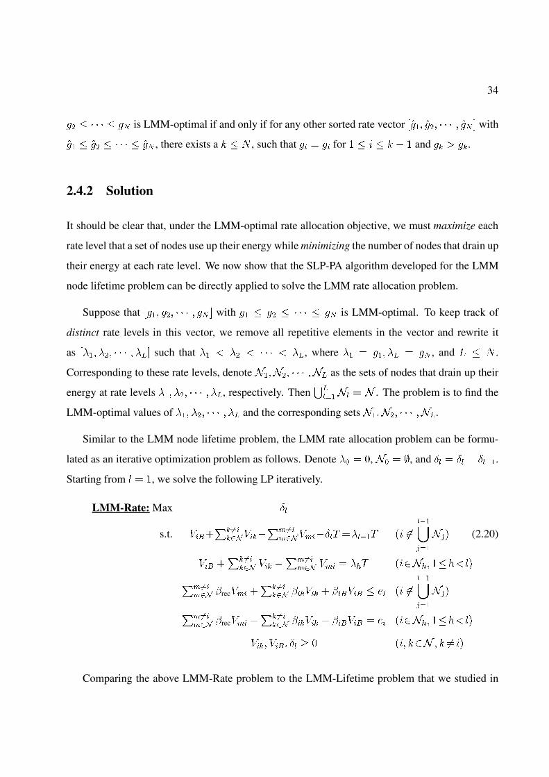
34

$� � � � � � $� is LMM-optimal if and only if for any other sorted rate vector �$�� $�� $� � with

�$� � �$� � � � � � �$� , there exists a � � � , such that $� � �$� for � � � � � � and $� � �$�.

2.4.2 Solution

It should be clear that, under the LMM-optimal rate allocation objective, we must maximize each

rate level that a set of nodes use up their energy while minimizing the number of nodes that drain up

their energy at each rate level. We now show that the SLP-PA algorithm developed for the LMM

node lifetime problem can be directly applied to solve the LMM rate allocation problem.

Suppose that $�� $�� $� � with $� � $� � � � � � $� is LMM-optimal. To keep track of

distinct rate levels in this vector, we remove all repetitive elements in the vector and rewrite it

as %�� %�� %�� such that %� � %� � � � � � %�, where %� � $�� %� � $� , and � � � .

Corresponding to these rate levels, denote �� as the sets of nodes that drain up their

energy at rate levels %�� %�� %�, respectively. Then��

�� . The problem is to find the

LMM-optimal values of %�� %�� %� and the corresponding sets �� .

Similar to the LMM node lifetime problem, the LMM rate allocation problem can be formu-

lated as an iterative optimization problem as follows. Denote %� � �, �� , and Æ � Æ � Æ��.

Starting from � � �, we solve the following LP iteratively.

LMM-Rate: Max Æ

s.t. ��

��

��Æ� �%��

�� (2.20)

��

��

�� %��

�� rec��

��

��

��

�� rec��

��

�� Æ � � � ��

Comparing the above LMM-Rate problem to the LMM-Lifetime problem that we studied in

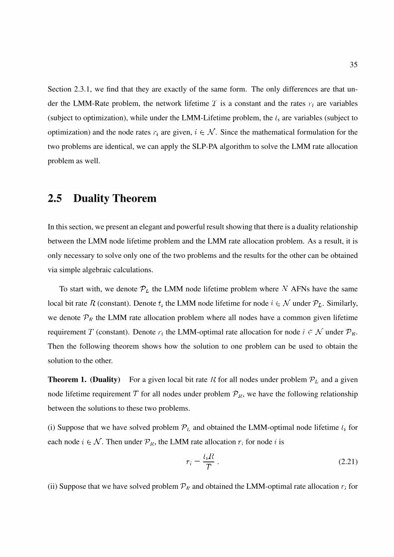
35

Section 2.3.1, we find that they are exactly of the same form. The only differences are that un-

der the LMM-Rate problem, the network lifetime � is a constant and the rates �� are variables

(subject to optimization), while under the LMM-Lifetime problem, the �� are variables (subject to

optimization) and the node rates �� are given, � . Since the mathematical formulation for the

two problems are identical, we can apply the SLP-PA algorithm to solve the LMM rate allocation

problem as well.

2.5 Duality Theorem

In this section, we present an elegant and powerful result showing that there is a duality relationship

between the LMM node lifetime problem and the LMM rate allocation problem. As a result, it is

only necessary to solve only one of the two problems and the results for the other can be obtained

via simple algebraic calculations.

To start with, we denote �� the LMM node lifetime problem where � AFNs have the same

local bit rate � (constant). Denote �� the LMM node lifetime for node � under ��. Similarly,

we denote �� the LMM rate allocation problem where all nodes have a common given lifetime

requirement � (constant). Denote �� the LMM-optimal rate allocation for node � under ��.

Then the following theorem shows how the solution to one problem can be used to obtain the

solution to the other.

Theorem 1. (Duality) For a given local bit rate � for all nodes under problem �� and a given

node lifetime requirement � for all nodes under problem ��, we have the following relationship

between the solutions to these two problems.

(i) Suppose that we have solved problem �� and obtained the LMM-optimal node lifetime �� for

each node � . Then under ��, the LMM rate allocation �� for node is

��

�� (2.21)

(ii) Suppose that we have solved problem �� and obtained the LMM-optimal rate allocation �� for

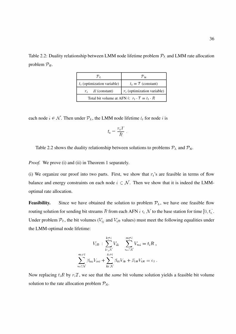
36

Table 2.2: Duality relationship between LMM node lifetime problem �� and LMM rate allocation

problem ��.

� ��

�� (optimization variable) �� (constant)

�� (constant) �� (optimization variable)

Total bit volume at AFN �: ��

each node � . Then under ��, the LMM node lifetime �� for node is

��

��

Table 2.2 shows the duality relationship between solutions to problems �� and ��.

Proof. We prove (i) and (ii) in Theorem 1 separately.

(i) We organize our proof into two parts. First, we show that ��’s are feasible in terms of flow

balance and energy constraints on each node � . Then we show that it is indeed the LMM-

optimal rate allocation.

Feasibility. Since we have obtained the solution to problem ��, we have one feasible flow

routing solution for sending bit streams � from each AFN � to the base station for time �� .

Under problem ��, the bit volumes (�� and �� values) must meet the following equalities under

the LMM-optimal node lifetime:

��

� ��

��

��

��

��

rec��

� ��

��

Now replacing �� by �� , we see that the same bit volume solution yields a feasible bit volume

solution to the rate allocation problem ��.

37

Optimality. To prove that ��’s obtained via (2.21) are indeed LMM-optimal for problem ��, we

sort ��’s in non-decreasing order and denote it as �� . We also introduce a node index

& � �� for �� . For example, � � means that � actually corresponds to

the lifetime of AFN �, i.e., � � ��.

Since �� is proportional to �� through the relationship (�� ), listing ��’s according to & �

�� will yield a sorted (in non-decreasing order) rate list, denoted as $�� $�� $� �.

We now prove that $�� $�� $� � is indeed LMM-optimal for problem ��.

Our proof is based on contradiction. Suppose that $�� $�� $� � is not LMM-optimal for

problem ��. Assume that the LMM-optimal rate vector to problem �� is �$�� $�� $� � (sorted

in non-decreasing order) with the corresponding node index being �& � � �� . Then, by

Definition 1, there exists a � � � such that �$ � $ for � � ' � � � � and �$� � $�.

We now claim that �� obtained via ��

, � �� , is also a feasible solution to

problem ��. The proof to this claim follows identically as above. Using this result, we can obtain

a corresponding feasible solution �� with ��

and the node index �& for problem

��. Hence we have ��

��

��

�� for � � ' � � � � but ��

��

�� . That is,

�� is not LMM-optimal and this leads to a contradiction.

(ii) The proof for this part follows the same token as the above proof for (i) and is thus omitted

here.

2.6 Numerical Investigation

In this section, we use numerical results to illustrate the solution of LMM node lifetime problem

and compare our SLP-PA to some other approaches. In particular, we will compare SLP-PA with

the naive approach (see Section 2.2) that uses a serial LP “blindly” to solve the LMM node lifetime

problem. We call this naive approach SLP-ER (serial LP with energy reservation). As discussed in

Section 2.2, the naive SLP-ER approach requires energy reservation at each stage and cannot give

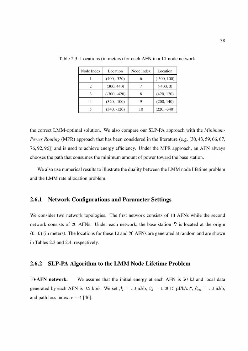
38

Table 2.3: Locations (in meters) for each AFN in a ��-node network.

Node Index Location Node Index Location

1 (400, -320) 6 (-500, 100)

2 (300, 440) 7 (-400, 0)

3 (-300, -420) 8 (420, 120)

4 (320, -100) 9 (200, 140)

5 (340, -120) 10 (220, -340)

the correct LMM-optimal solution. We also compare our SLP-PA approach with the Minimum-

Power Routing (MPR) approach that has been considered in the literature (e.g. [30, 43, 59, 66, 67,

76, 92, 96]) and is used to achieve energy efficiency. Under the MPR approach, an AFN always

chooses the path that consumes the minimum amount of power toward the base station.

We also use numerical results to illustrate the duality between the LMM node lifetime problem

and the LMM rate allocation problem.

2.6.1 Network Configurations and Parameter Settings

We consider two network topologies. The first network consists of �� AFNs while the second

network consists of �� AFNs. Under each network, the base station ( is located at the origin

�� (in meters). The locations for these �� and �� AFNs are generated at random and are shown

in Tables 2.3 and 2.4, respectively.

2.6.2 SLP-PA Algorithm to the LMM Node Lifetime Problem

��-AFN network. We assume that the initial energy at each AFN is �� kJ and local data

generated by each AFN is �� kb/s. We set � � �� nJ/b, � � �� pJ/b/!�, rec � �� nJ/b,

and path loss index � � � [46].

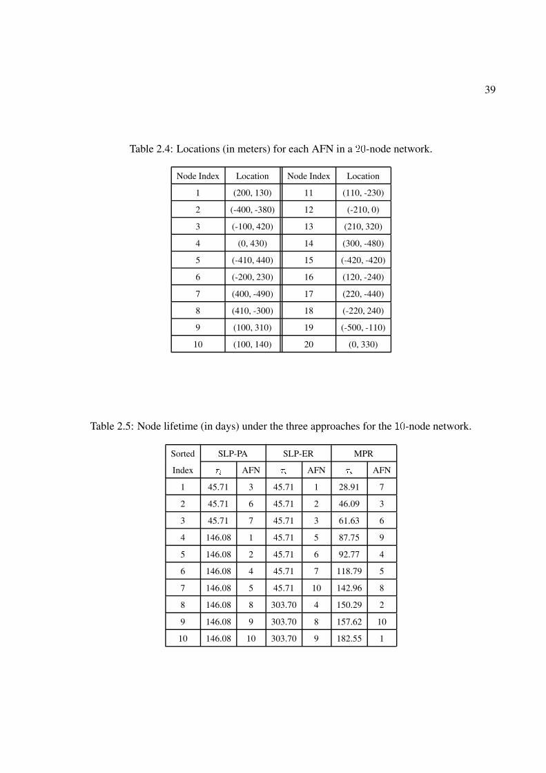
39

Table 2.4: Locations (in meters) for each AFN in a ��-node network.

Node Index Location Node Index Location

1 (200, 130) 11 (110, -230)

2 (-400, -380) 12 (-210, 0)

3 (-100, 420) 13 (210, 320)

4 (0, 430) 14 (300, -480)

5 (-410, 440) 15 (-420, -420)

6 (-200, 230) 16 (120, -240)

7 (400, -490) 17 (220, -440)

8 (410, -300) 18 (-220, 240)

9 (100, 310) 19 (-500, -110)

10 (100, 140) 20 (0, 330)

Table 2.5: Node lifetime (in days) under the three approaches for the ��-node network.

Sorted SLP-PA SLP-ER MPR

Index � AFN � AFN � AFN

1 45.71 3 45.71 1 28.91 7

2 45.71 6 45.71 2 46.09 3

3 45.71 7 45.71 3 61.63 6

4 146.08 1 45.71 5 87.75 9

5 146.08 2 45.71 6 92.77 4

6 146.08 4 45.71 7 118.79 5

7 146.08 5 45.71 10 142.96 8

8 146.08 8 303.70 4 150.29 2

9 146.08 9 303.70 8 157.62 10

10 146.08 10 303.70 9 182.55 1

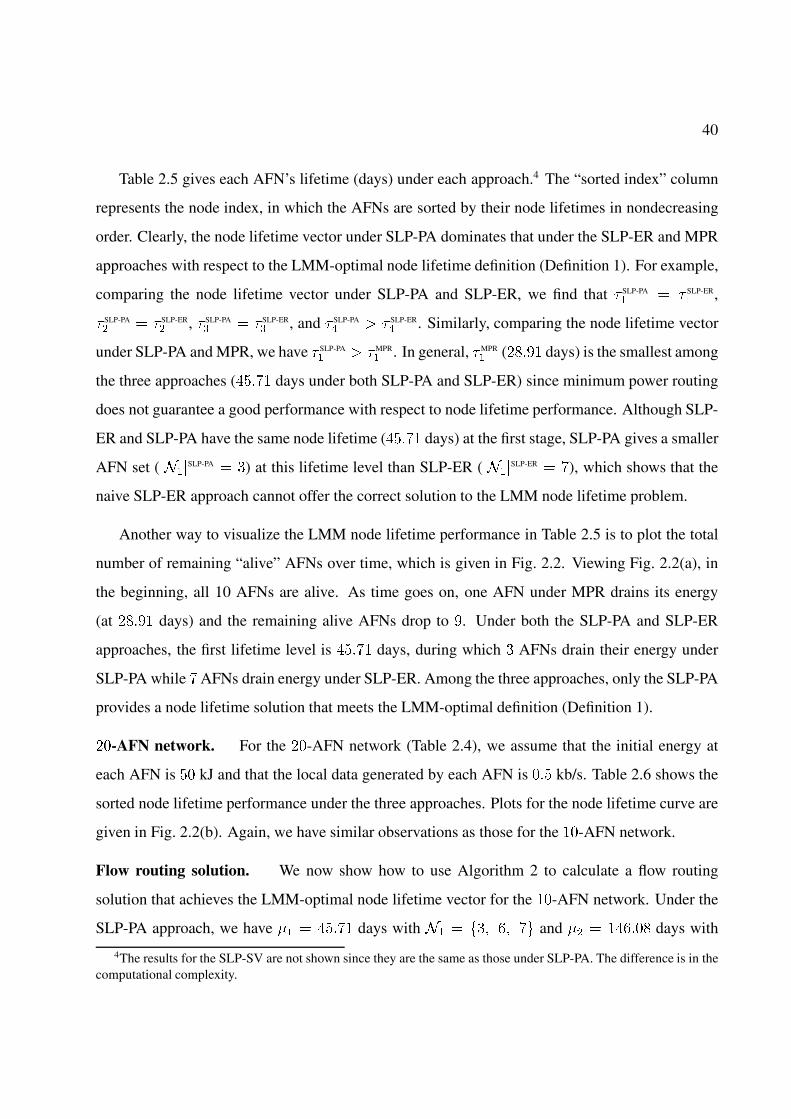
40

Table 2.5 gives each AFN’s lifetime (days) under each approach.4 The “sorted index” column

represents the node index, in which the AFNs are sorted by their node lifetimes in nondecreasing

order. Clearly, the node lifetime vector under SLP-PA dominates that under the SLP-ER and MPR

approaches with respect to the LMM-optimal node lifetime definition (Definition 1). For example,

comparing the node lifetime vector under SLP-PA and SLP-ER, we find that � SLP-PA� � � SLP-ER

� ,

� SLP-PA� � � SLP-ER

� , � SLP-PA � � SLP-ER

, and � SLP-PA� � � SLP-ER

� . Similarly, comparing the node lifetime vector

under SLP-PA and MPR, we have � SLP-PA� � �MPR

� . In general, �MPR� (�� days) is the smallest among

the three approaches (�� days under both SLP-PA and SLP-ER) since minimum power routing

does not guarantee a good performance with respect to node lifetime performance. Although SLP-

ER and SLP-PA have the same node lifetime (�� days) at the first stage, SLP-PA gives a smaller

AFN set ( �� SLP-PA � ) at this lifetime level than SLP-ER ( ��

SLP-ER � �), which shows that the

naive SLP-ER approach cannot offer the correct solution to the LMM node lifetime problem.

Another way to visualize the LMM node lifetime performance in Table 2.5 is to plot the total

number of remaining “alive” AFNs over time, which is given in Fig. 2.2. Viewing Fig. 2.2(a), in

the beginning, all 10 AFNs are alive. As time goes on, one AFN under MPR drains its energy

(at �� days) and the remaining alive AFNs drop to �. Under both the SLP-PA and SLP-ER

approaches, the first lifetime level is �� days, during which AFNs drain their energy under

SLP-PA while � AFNs drain energy under SLP-ER. Among the three approaches, only the SLP-PA

provides a node lifetime solution that meets the LMM-optimal definition (Definition 1).

��-AFN network. For the ��-AFN network (Table 2.4), we assume that the initial energy at

each AFN is �� kJ and that the local data generated by each AFN is �� kb/s. Table 2.6 shows the

sorted node lifetime performance under the three approaches. Plots for the node lifetime curve are

given in Fig. 2.2(b). Again, we have similar observations as those for the ��-AFN network.

Flow routing solution. We now show how to use Algorithm 2 to calculate a flow routing

solution that achieves the LMM-optimal node lifetime vector for the ��-AFN network. Under the

SLP-PA approach, we have �� days with �� and �� days with

4The results for the SLP-SV are not shown since they are the same as those under SLP-PA. The difference is in thecomputational complexity.

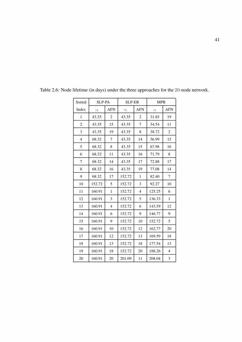
41

Table 2.6: Node lifetime (in days) under the three approaches for the ��-node network.

Sorted SLP-PA SLP-ER MPR

Index � AFN � AFN � AFN

1 43.35 2 43.35 2 31.85 19

2 43.35 15 43.35 7 34.54 11

3 43.35 19 43.35 8 38.72 2

4 68.32 7 43.35 14 56.99 15

5 68.32 8 43.35 15 67.98 16

6 68.32 11 43.35 16 71.79 8

7 68.32 14 43.35 17 72.88 17

8 68.32 16 43.35 19 77.08 14

9 68.32 17 152.72 1 82.40 7

10 152.72 5 152.72 3 92.27 10

11 160.91 1 152.72 4 125.25 6

12 160.91 3 152.72 5 136.33 1

13 160.91 4 152.72 6 143.59 12

14 160.91 6 152.72 9 146.77 9

15 160.91 9 152.72 10 152.72 5

16 160.91 10 152.72 12 162.77 20

17 160.91 12 152.72 13 169.59 18

18 160.91 13 152.72 18 177.54 13

19 160.91 18 152.72 20 188.26 4

20 160.91 20 201.09 11 208.04 3

42

0 30 60 90 120 150 180 210 240 270 300 3300

1

2

3

4

5

6

7

8

9

10

11

12

Node Lifetime (days)

Num

ber

of A

live

Nod

es

SLP−ER

MPR

SLP−PA

(a) ��-node network.

0 20 40 60 80 100 120 140 160 180 200 2200

2

4

6

8

10

12

14

16

18

20

22

Node Lifetime (days)

Num

ber

of A

live

Nod

es

SLP−ER

MPR

SLP−PA

(b) �-node network.

Figure 2.2: Node lifetime curves under the three approaches.

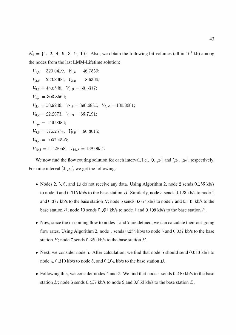
43

�� . Also, we obtain the following bit volumes (all in �� kb) among

the nodes from the last LMM-Lifetime solution:

�� , �� ;

�� , �� ;

�� , �� ;

�� ;

�� , �� , �� ;

�� , �� ;

�� ;

�� , �� ;

� �� ;

�� , �� .

We now find the flow routing solution for each interval, i.e., �� and �� , respectively.

For time interval �� , we get the following.

� Nodes �, , �, and �� do not receive any data. Using Algorithm 2, node � sends �� kb/s

to node � and �� kb/s to the base station (. Similarly, node sends �� kb/s to node �

and �� kb/s to the base station (; node � sends �� kb/s to node � and �� kb/s to the

base station (; node �� sends �� kb/s to node � and �� kb/s to the base station (.

� Now, since the in-coming flow to nodes � and � are defined, we can calculate their out-going

flow rates. Using Algorithm 2, node � sends �� kb/s to node � and �� kb/s to the base

station (; node � sends �� kb/s to the base station (.

� Next, we consider node �. After calculation, we find that node � should send �� kb/s to

node �, �� kb/s to node �, and �� kb/s to the base station (.

� Following this, we consider nodes � and �. We find that node � sends �� kb/s to the base

station (; node � sends �� kb/s to node � and �� kb/s to the base station (.

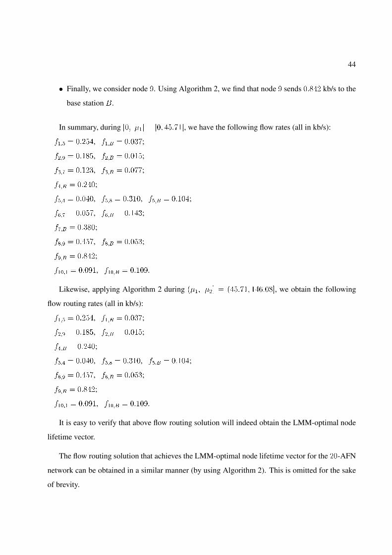
44

� Finally, we consider node �. Using Algorithm 2, we find that node � sends �� kb/s to the

base station (.

In summary, during �� , we have the following flow rates (all in kb/s):

�� , �� ;

�� , �� ;

�� , �� ;

�� ;

�� , �� , �� ;

�� , �� ;

�� ;

�� , �� ;

� �� ;

�� , �� .

Likewise, applying Algorithm 2 during �� , we obtain the following

flow routing rates (all in kb/s):

�� , �� ;

�� , �� ;

�� ;

�� , �� , �� ;

�� , �� ;

� �� ;

�� , �� .

It is easy to verify that above flow routing solution will indeed obtain the LMM-optimal node

lifetime vector.

The flow routing solution that achieves the LMM-optimal node lifetime vector for the ��-AFN

network can be obtained in a similar manner (by using Algorithm 2). This is omitted for the sake

of brevity.

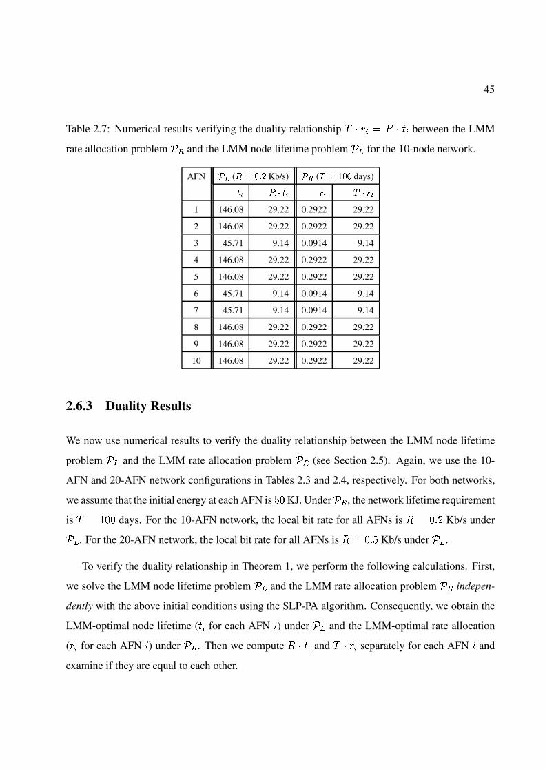
45

Table 2.7: Numerical results verifying the duality relationship � � �� between the LMM

rate allocation problem �� and the LMM node lifetime problem �� for the 10-node network.

AFN � ( � �# Kb/s) �� ( � �� days)

��

1 146.08 29.22 0.2922 29.22

2 146.08 29.22 0.2922 29.22

3 45.71 9.14 0.0914 9.14

4 146.08 29.22 0.2922 29.22

5 146.08 29.22 0.2922 29.22

6 45.71 9.14 0.0914 9.14

7 45.71 9.14 0.0914 9.14

8 146.08 29.22 0.2922 29.22

9 146.08 29.22 0.2922 29.22

10 146.08 29.22 0.2922 29.22

2.6.3 Duality Results

We now use numerical results to verify the duality relationship between the LMM node lifetime

problem �� and the LMM rate allocation problem �� (see Section 2.5). Again, we use the 10-

AFN and 20-AFN network configurations in Tables 2.3 and 2.4, respectively. For both networks,

we assume that the initial energy at each AFN is �� KJ. Under��, the network lifetime requirement

is � � �� days. For the 10-AFN network, the local bit rate for all AFNs is � � �� Kb/s under

��. For the 20-AFN network, the local bit rate for all AFNs is � � �� Kb/s under ��.

To verify the duality relationship in Theorem 1, we perform the following calculations. First,

we solve the LMM node lifetime problem �� and the LMM rate allocation problem �� indepen-

dently with the above initial conditions using the SLP-PA algorithm. Consequently, we obtain the

LMM-optimal node lifetime (�� for each AFN ) under �� and the LMM-optimal rate allocation

(�� for each AFN ) under ��. Then we compute � � �� and � � �� separately for each AFN and

examine if they are equal to each other.

46

Table 2.8: Numerical results verifying the duality relationship � � �� between the LMM

rate allocation problem �� and the LMM node lifetime problem �� for the 20-node network.

AFN � ( � �#� Kb/s) �� ( � �� days)

��

1 160.91 80.46 0.8046 80.46

2 43.35 21.68 0.2168 21.68

3 160.91 80.46 0.8046 80.46

4 160.91 80.46 0.8046 80.46

5 152.72 76.36 0.7636 76.36

6 160.91 80.46 0.8046 80.46

7 68.32 34.16 0.3416 34.16

8 68.32 34.16 0.3416 34.16

9 160.91 80.46 0.8046 80.46

10 160.91 80.46 0.8046 80.46

11 68.32 34.16 0.3416 34.16

12 160.91 80.46 0.8046 80.46

13 160.91 80.46 0.8046 80.46

14 68.32 34.16 0.3416 34.16

15 43.35 21.68 0.2168 21.68

16 68.32 34.16 0.3416 34.16

17 68.32 34.16 0.3416 34.16

18 160.91 80.46 0.8046 80.46

19 43.35 21.68 0.2168 21.68

20 160.91 80.46 0.8046 80.46

47

The results for the LMM-optimal node lifetime (��, � �� ) and the LMM-optimal

rate allocation (��, � �� ) for the ��-AFN network are shown in Table 2.7. We find that

� � �� and � � �� are exactly equal for all AFNs, precisely as we would expect under Theorem 1.

Similarly, the results for the 20-AFN network are shown in Table 2.8.

2.7 Related Work

Due to energy constraints in wireless sensor networks, there has been active research on exploring

the performance limits of such networks. These performance limits include, among others, network

lifetime and network capacity. Network lifetime refers to the maximum time that the nodes in

the network remain alive before one or more nodes deplete their energy, while network capacity

typically refers to the maximum amount of bit volume that can be successfully delivered to the

base station (“sink node”) by all the nodes in the network.

The network lifetime problem and network capacity problem have so far been studied disjointly

in the literature. For example, in many other efforts (e.g., [11, 13, 18, 55, 115]), the focus was on

how to maximize the time until the first node drains up its energy. While, in [56], the problem of

how to maximize network capacity via routing was studied.

In this chapter, we study the important overarching problem that considers both network life-

time and network capacity. The notion of network lifetime for wireless sensor networks has been

studied in [10, 11, 13, 17–19, 55, 115]. The notion of network lifetime discussed in these work fo-

cuses on the time until the first node fails without further consideration of the remaining nodes in

the network. As wireless sensor networks will typically remain useful even if some nodes run out

of energy, it is essential to further investigate how to maximize the lifetime for all the remaining

nodes in the network, which is the focus of the LMM node lifetime problem. Under the LMM

node lifetime problem, we studied how to maximize the lifetime for all nodes when the local bit

rate for each node is given. The closest work related to the LMM node lifetime problem is that

in [15], which has been discussed in detail in this chapter.

48

Under the LMM rate allocation problem, we studied how to maximize rate allocations for all

the nodes in the network under a given network lifetime requirement. The LMM rate allocation

criterion effectively mitigates the unfairness issue when the objective is to maximize the total bit

volume generated by the network. Although the LMM rate allocation is somewhat similar to the

classical max-min strategy [9], there is a fundamental difference between the two. In particular,

the LMM rate allocation problem implicitly embeds (or couples) a flow routing problem within

rate allocation, while under the classical max-min rate allocation, there is no routing problem

involved since the routes for all flows are given. Due to this coupling of flow routing and rate

allocation, a solution approach (i.e., SLP-PA) to the LMM rate allocation problem is much more

challenging than that for the classical max-min. In [94], Srinivasan et al. applied game theory and

Nash equilibrium among the nodes to forward packets such that the total throughput (capacity)

can achieve an optimal operating point subject to a common lifetime requirement on all nodes.

However, the fairness issue in information collection was not considered.

2.8 Conclusions

In this chapter, we considered the problem of how to maximize the lifetime for all the nodes in a

wireless sensor network. We formally defined this optimization problem as the lexicographic max-

min (LMM) node lifetime problem and investigated approaches to solve it. The main contributions

in this problem are two-fold. First, we developed a polynomial-time algorithm to obtain the LMM-

optimal node lifetime vector, which improves upon the computational complexity associated with

a state-of-the-art algorithm. Second, we discussed how to obtain the routing solution among the

AFNs such that the LMM-optimal node lifetime vector can be achieved. We show that the SLP-PA

can also be employed to address the LMM rate allocation problem. More important, we discovered

a simple and elegant duality relationship between the LMM node lifetime problem and the LMM

rate allocation problem, which enables us to develop solutions and insights on both problems

by solving one of the two problems. The results in this chapter help lay the essential algorithmic

foundation for studying network lifetime problems in energy-constrained wireless sensor networks.

Chapter 3

Base Station Placement for Wireless Sensor

Networks

3.1 Introduction

An important characteristic for wireless sensor networks is the so-called network lifetime perfor-

mance, which is highly dependent upon the physical topology of the network. This is because

energy expenditure at a node to transmit data to another node not only depends on the data bit

rate, but also on the physical distance between these two nodes. Consequently, it is important to

understand the impact of location related issues on network lifetime performance and to optimize

topology during network deployment stage.

This chapter considers the important problem of base station placement for a given sensor

network such that network lifetime can be maximized. Specifically, we consider the following

problem. Given a sensor network with each node producing data at a rate of ��, where should

we place the base station in this sensor network such that all the data can be forwarded to the base

station (via multi-hop and multi-path if necessary) such that the network lifetime is maximized?

In Section 3.5, we give a comprehensive review of related work on network lifetime and node

49

50

placement problems and contrast their differences with this work. The most important work on this

problem is done by Efrat et al. [32], which represents the state-of-the-art result on this problem.

However, the computational complexity associated with the algorithm in [32] is higher than the

one to be presented in this chapter for most cases.

The main idea in our approximation algorithm is to exploit a clever way to discretize cost

parameters associated with energy consumption with tight upper and lower bounds. As a result, we

can divide the continuous search space into a finite number of subareas. By further exploiting the

cost property of each subarea, we conceive a novel idea to represent each subarea with a so-called

“fictitious cost point” (FCP), which is an � -tuple cost vector with each component representing the

upper bound of cost to a sensor node in the network. Based on these ideas, we have successfully

reduced an infinite search space for base station location into a finite “points” upon which we

can apply a linear program (LP) to find the corresponding achievable network lifetime and data

routing solution. By comparing the achievable network lifetime among all the FCPs, we show

that the largest one is �� -optimal. We also prove that locating the base station at any point

in the subarea corresponding to the best FCP is �� -optimal. We analyze the complexity of

our approximation algorithm and show that it is practically faster than the algorithm proposed

in [32] for most cases, which was the best known result on this problem. As a result, the algorithm

presented in this chapter represents the best known result to the base station placement problem.

The remainder of the chapter is organized as follows. Section 3.2 presents the network model

used in this study and describes the base station placement problem. Section 3.3 presents the main

result of this chapter, which is a �� -approximation algorithm for the base station placement

problem. In Section 3.4, we present some numerical results illustrating the efficacy of the proposed

algorithm. Section 3.5 reviews related work and Section 3.6 concludes this chapter.

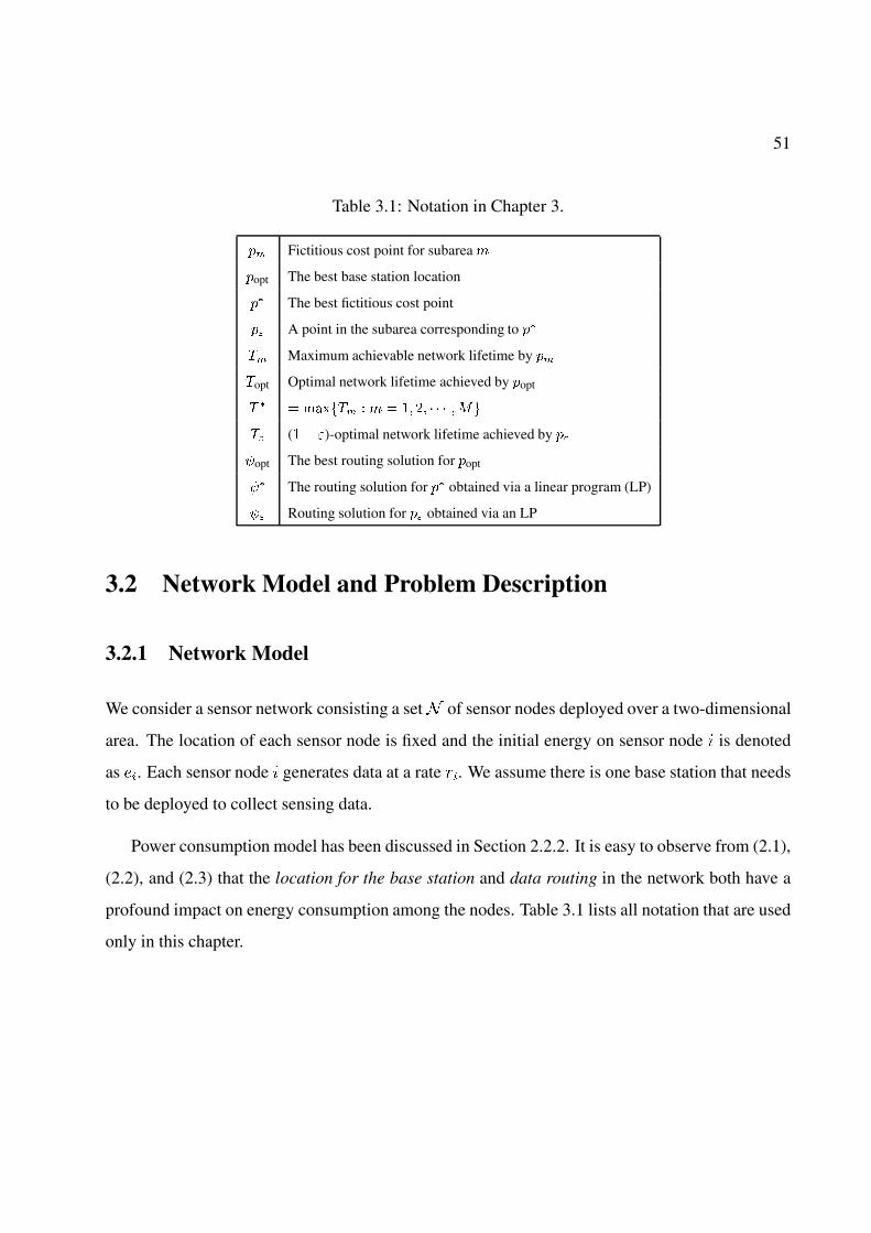
51


�� Fictitious cost point for subarea �

�opt The best base station location

�� The best fictitious cost point

�� A point in the subarea corresponding to ��

� Maximum achievable network lifetime by ��

opt Optimal network lifetime achieved by �opt

� � � ��

� (�� )-optimal network lifetime achieved by ��

�opt The best routing solution for �opt

�� The routing solution for �� obtained via a linear program (LP)

�� Routing solution for �� obtained via an LP

3.2 Network Model and Problem Description

3.2.1 Network Model

We consider a sensor network consisting a set� of sensor nodes deployed over a two-dimensional

area. The location of each sensor node is fixed and the initial energy on sensor node is denoted

as ��. Each sensor node generates data at a rate ��. We assume there is one base station that needs

to be deployed to collect sensing data.

Power consumption model has been discussed in Section 2.2.2. It is easy to observe from (2.1),

(2.2), and (2.3) that the location for the base station and data routing in the network both have a

profound impact on energy consumption among the nodes. Table 3.1 lists all notation that are used

only in this chapter.

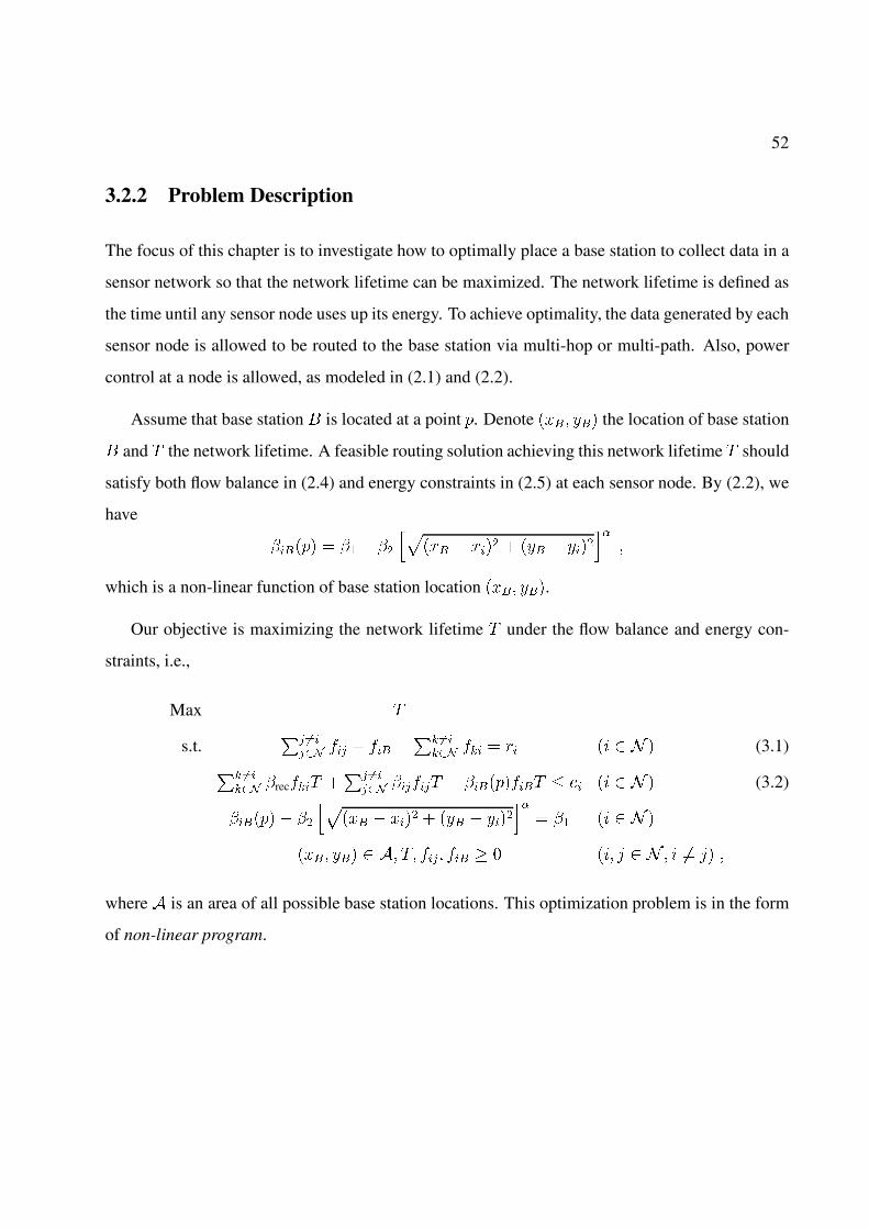
52

3.2.2 Problem Description

The focus of this chapter is to investigate how to optimally place a base station to collect data in a

sensor network so that the network lifetime can be maximized. The network lifetime is defined as

the time until any sensor node uses up its energy. To achieve optimality, the data generated by each

sensor node is allowed to be routed to the base station via multi-hop or multi-path. Also, power

control at a node is allowed, as modeled in (2.1) and (2.2).

Assume that base station ( is located at a point . Denote �� )�� the location of base station

( and � the network lifetime. A feasible routing solution achieving this network lifetime � should

satisfy both flow balance in (2.4) and energy constraints in (2.5) at each sensor node. By (2.2), we

have

��

�� )� � )��

��

which is a non-linear function of base station location �� )��.

Our objective is maximizing the network lifetime � under the flow balance and energy con-

straints, i.e.,

Max �

s.t.� ��

��

�� (3.1)�� rec��

� �� (3.2)

��

�� )� � )��

��

�� )�� ' � � �� '� �

where � is an area of all possible base station locations. This optimization problem is in the form

of non-linear program.

53

3.3 An Approximation Algorithm

3.3.1 Our Approach

As discussed earlier, network lifetime depends on both base station location and data routing. To

start with, we show that for a given base station location, we can find the corresponding maximum

achievable network lifetime and optimal routing via a single linear program (LP) as follows.

The objective function is network lifetime � and the constraints are given in (3.1) and (3.2).

Multiply both sides of (3.1) by � and denote �� and �� , where �� (or ��) can

be interpreted as the total data volume from sensor node to sensor node ' (or base station (). We

have

Max �

s.t.��

��

�� rec��

� ��

�� ' � � �� '�

It should be note that for a given base station location, ��’s are constants. Once we solve the

above LP, we can obtain optimal routing solution for �� and �� by ��

and ��

.

Although for a given base station location, we can find the corresponding maximum achievable

network lifetime via a single LP, it is not possible to examine all points (infinite) in the two-

dimensional plane and select the point with the maximum network lifetime among all the points.

Our approach to this search problem is to narrow down the search space to a finite set of points,

among which there exist at least one point with �� -optimal network lifetime.

As a first step, we show that it is only necessary to consider points inside the so-called smallest

enclosing disk (SED) [106],1 which is a unique disk with the smallest radius that contains all the

1In fact, we can consider points in an even smaller area, i.e., the convex hull of all sensor nodes. However, usingconvex hull cannot reduce the order of complexity of our algorithm. On the other hand, the use of SED can simplifythe discussion.

54

A

OA

pi

q

R

Figure 3.1: A schematic diagram showing that optimal base station location must be within SED.

� sensor nodes in the network and can be found in #�� time [25]. This is formally stated in the

following lemma.

Lemma 3. To maximize network lifetime, the base station location must be within the smallest

enclosing disk� that covers all sensor nodes in the network.

Proof. The proof is based on contradiction. That is, if the base station location is not in SED, then

its network lifetime can be further increased and thus this location cannot be maximum.

Assume that the optimal base station location is at point , which is outside SED �. Denote

#� the center of SED (see Fig. 3.1). Let be the intersecting point between the line segment

� #�� and the circle of SED. Then for any sensor (all in �), we have �� . Consequently,

�� . As a result, we can save transmission energy on every sensor node � by relocating

to and thereby increase network lifetime. This completes the proof.

Now we have narrowed down the search space for base station ( from a two-dimensional plane

to SED �. However, the number of points in � remains infinite. It is tempting to divide � into

55

small subareas (e.g., a grid-like structure), �� , up to say �� , i.e.,

� ��

��

��

When each subarea is sufficiently small (i.e., * is sufficiently large), we can use some point

� �� to represent ��, ! � �� * . By applying an LP on each of the * points, we

can find the best location and obtain a good solution for base station placement. However, such

approach is heuristic at best and does not provide any theoretical guarantee on performance.

The key to provide a theoretical guarantee on performance is to divide SED � in such a way

that certain bounds can be imposed on any point in a subarea. If this is possible, then we can ex-

ploit such properties and develop an approximation algorithm that yields provably �� -optimal

network lifetime performance. In the following section, we show a novel technique to divide SED

� into subareas where each subarea can be represented by a point with a set of tight bounds.

Consequently, a �� -optimal approximation algorithm can be developed.

3.3.2 Subarea Division and Fictitious Cost Points

Subarea Division

The proposed subarea division (with guaranteed performance bounds) hinges upon discretization

of the cost parameters. A close look at the energy constraint in (3.2) suggests that the location of

the base station is embedded in the cost parameter ��’s. In other words, if we can discretize

these cost parameters, we may also discretize the location for the base station.

Since the search space is narrowed down to the SED �, we can limit the range for the distance

between a sensor node to the possible location for the base station. Denote #� and �� the origin

and radius of the SED �. For each sensor node � , denote �� the distance from sensor

node to the origin of disk � (see node 4 in Fig. 3.2 as an example). Denote �min�� and �max

�� the

minimum and maximum distances between sensor node and possible location for the base station

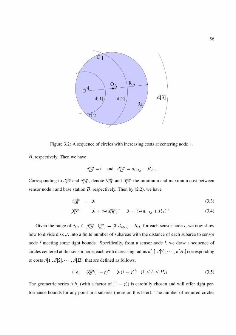
56

OARA

4

1

2

3d[1] d[2] d[3]

Figure 3.2: A sequence of circles with increasing costs at centering node �.

(, respectively. Then we have

�min�� and �max

��

Corresponding to �min�� and �max

�� , denote min�� and max

�� the minimum and maximum cost between

sensor node and base station (, respectively. Then by (2.2), we have

min�� (3.3)

max��

max��

� � (3.4)

Given the range of �� min�� max

�� for each sensor node , we now show

how to divide disk � into a finite number of subareas with the distance of each subarea to sensor

node meeting some tight bounds. Specifically, from a sensor node , we draw a sequence of

circles centered at this sensor node, each with increasing radius � �� +�� corresponding

to costs �� +�� that are defined as follows.

�� min�� +�� (3.5)

The geometric series �� (with a factor of �� ) is carefully chosen and will offer tight per-

formance bounds for any point in a subarea (more on this later). The number of required circles

57

+� can be determined by having the last circle in the sequence (with radius � +��) to completely

contain disk �, i.e. � +�� max�� , or equivalently, +�� max

�� . This will set the limit +� as

+� �

��max

�� ,min��

��

��

��

��

��

��

�� (3.6)

For example, for node � in Fig. 3.2, we have +� � , i.e., � � is the circle centered at node � that

will completely contain the disk. As a result, with sensor node as center, we have a total of +�

circles, each with cost ��, � � �� +�.

The above partitioning of SED � is in respect to a specific node . We now perform the above

process for all sensor nodes. These intersecting circles will cut disk � into a finite number of

non-uniform subareas, with the boundaries of each subarea being either an arc (with a center at

some sensor node and some cost ��, � � � � +�) or an arc from SED �. As an example, the

SED � in Fig. 3.3 is now divided into �� subareas.

Now we claim that under this subarea partitioning technique, for any point in a given subarea,

its cost to each sensor node in the network can be tightly bounded. This is because with respect to

each sensor node , a subarea �� must be enclosed within some ring centered at at sensor node .

Denote the index of this ring (w.r.t. sensor node ) as ��. So when the base station ( is at any

point ��, we have

�� (3.7)

where we define �� min�� . Since ��

�� by (3.5), we have a very tight upper

and lower bounds for �� (now we see the benefit of our discretization technique for cost and

distance).

Fictitious Cost Point

We now introduce a novel concept called fictitious cost point (FCP). It will be used to represent

upper bound of cost for any point in a subarea ��, ! � �� * .

58

4

q3q1

1

2

3

q2

Figure 3.3: An example of subareas within disk � that are obtained by intersecting arcs from

different circles.

Definition 3. Denote the fictitious cost point for subarea �� (! � �� * ) as �, which is

represented by an � -tuple vector �� , with its -th element ( � )

being upper cost bound for any point in subarea �� to sensor node , i.e.,

�� (3.8)

where �� is determined by (3.7).

As an example, the FCP for subarea with corner points � �� in Fig. 3.3 can be represented

by �-tuple cost vector �� , where the

first component �� represents an upper bound of cost for any point in this subarea to sensor node

�, the second component � represents an upper bound of cost (which is loose here) for any point

in this subarea to sensor node �, and so forth.

We emphasize that the reason we use the word “fictitious” is that an FCP � may not be

59

mapped to a physical point within the corresponding subarea ��. This happens when there does

not exist a physical point in subarea �� that has its costs to all the � sensor nodes equal (one

by one) to the respective � -tuple cost vector embodied by � simultaneously. As an example,

any point within the dark subarea bounded by corner points �, �, and cannot have its costs

to the four sensor nodes in the network equal to the respective element in ��

simultaneously, where �� is the cost vector of the FCP for this subarea.

Using “fictitious” points to represent subareas and to construct a finite search space is a key

step in design our low complexity approximation algorithm. As a contrast, in [32], the authors

use physical points to construct a finite search space. Thus, they cannot discretize cost directly.

Instead, they consider how to discretize transmission energy, flow rate, and network lifetime such

that cost can be discretized. The number of discretized costs is the product of the numbers of dis-

cretized transmission energies, flow rates, and network lifetimes. We will show that the complexity

associated with the algorithm in [32] is higher than ours for most cases.

The following important property for FCP � will be used in the proof of �� -optimality

of the approximation algorithm.

Property 1. Denote � the FCP for subarea ��, ! � �� * . For any point ��, we

have

��

Proof. By definition of FCP � in (3.8), we have

��

��

��

��

��

��

��

��

where the inequality follows from (3.7). This completes the proof.

3.3.3 Summary of Algorithm and Example

By discretizing the cost parameters and the corresponding distances, we have partitioned the search

space (SED �) into a finite number (* ) subareas. By introducing the concept of FCP, we can

60

represent each subarea with a point. As a result, we can now readily apply the LP approach

discussed in Section 3.3.1 to examine each point and choose the point that offers the maximum

network lifetime. The complete approximation algorithm is outlined below. The correctness proof

of �� -optimality is given in Section 3.3.4.

Algorithm 3. (A �� -Approximation Algorithm)

1. Find the smallest enclosing disk � that covers all � nodes.

2. Within �, compute the lower and upper cost bounds min�� and max

�� for each node � by

(3.3) and (3.4).

3. For a given � � �, define a sequence of costs ��, �� +�� by (3.5), where +� can

by calculated by (3.6).

4. For each node , draw a sequence of +� � � circles corresponding to cost �� centered at

node , � � � � +�. The intersection of these circles within disk � will divide � into *

subareas ��, �� .

5. For each subarea ��, � � ! � * , define an FCP �, which embodies an � -tuple cost

vector �� , where �� is defined in (3.8).

6. For each of these * FCPs, apply the LP in Section 3.3.1 and obtain the maximum achievable

network lifetime.

7. Choose the FCP that offers the maximum network lifetime among these * FCPs. The

base station can be placed at any point � within the subarea corresponding to .

8. For point �, apply the LP in Section 3.3.1 and obtain a routing solution -� with �� -

optimal network lifetime ��.

Remark. Note that the above algorithm can be easily extended to accommodate any additional

area constraint on base station placement. That is, we can define � in Step � to be the intersection

between SED and the allowed area for base station placement.

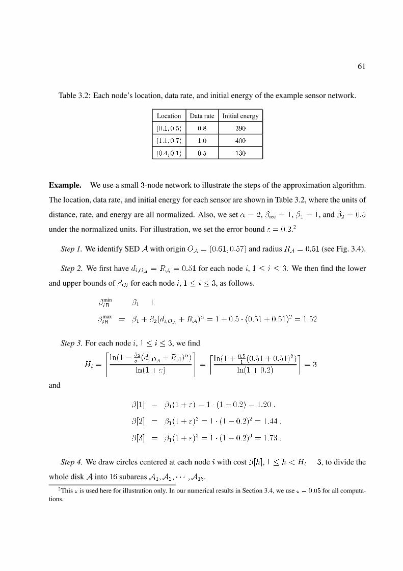
61

Table 3.2: Each node’s location, data rate, and initial energy of the example sensor network.

Location Data rate Initial energy

��#�� #�� #� ��

��#�� #�� #� ��

��#�� #�� #� ��

Example. We use a small -node network to illustrate the steps of the approximation algorithm.

The location, data rate, and initial energy for each sensor are shown in Table 3.2, where the units of

distance, rate, and energy are all normalized. Also, we set � � �, rec � �, � � �, and � � ��

under the normalized units. For illustration, we set the error bound � � ��.2

Step 1. We identify SED� with origin #� � �� and radius �� (see Fig. 3.4).

Step 2. We first have �� for each node , � � � . We then find the lower

and upper bounds of �� for each node , � � � , as follows.

min��

max��

� � � � ��

Step 3. For each node , � � � , we find

+� �

��

��

��

��

��

��

��

��

��

and

��

��

� � ��

Step 4. We draw circles centered at each node with cost ��, � � � � +� � , to divide the

whole disk � into �� subareas �� .2This � is used here for illustration only. In our numerical results in Section 3.4, we use � � �#�� for all computa-

tions.

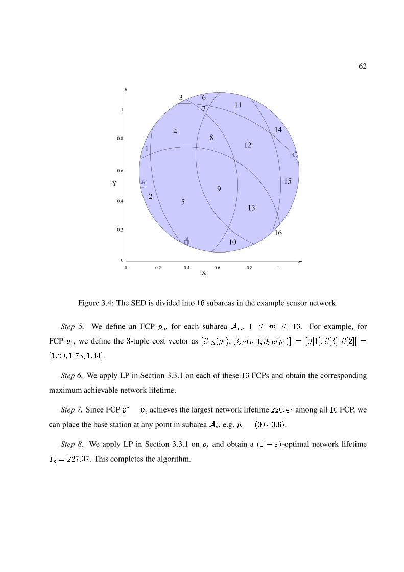
62

0 0.2 0.4 0.6X

0.8 1

0

0.2

0.4

0.6

0.8

1

Y

3

4

5

6

7

8

9

10

11

12

13

14

15

16

1

2

Figure 3.4: The SED is divided into �� subareas in the example sensor network.

Step 5. We define an FCP � for each subarea ��, � � ! � ��. For example, for

FCP �, we define the -tuple cost vector as ��, ��

�� .

Step 6. We apply LP in Section 3.3.1 on each of these �� FCPs and obtain the corresponding

maximum achievable network lifetime.

Step 7. Since FCP � achieves the largest network lifetime �� among all �� FCP, we

can place the base station at any point in subarea � , e.g. � � �� .

Step 8. We apply LP in Section 3.3.1 on � and obtain a �� -optimal network lifetime

�� . This completes the algorithm.

63

3.3.4 Proof and Complexity Analysis

In this section, we give a formal proof that the solution obtained by Algorithm 3 is �� -optimal

and analyze its complexity.

Denote opt the optimal location for base station placement and �opt and -opt the correspond-

ing maximum network lifetime and data routing solution, all of which are unknown. Denote

the best FCP among the * FCPs, based on their maximum achievable network lifetime perfor-

mance. Denote � and - the corresponding network lifetime and data routing solution, i.e.,

� � �� ! � �� *�.

Based on Step 7 in Algorithm 3, we choose a physical point � in the subarea corresponding to

for base station placement. For point �, denote the maximum achievable network lifetime as

�� and corresponding routing solution as -�.

Our roadmap for the proof is as follows. In Theorem 2, we will prove that � for the best FCP

is at least �� of the optimum, i.e., � �� opt. Subsequently, in Theorem 3, we will

show that for the physical point �, the corresponding network lifetime �� is also at least ��

of the optimum, i.e., �� opt.

Theorem 2. For � and �opt as defined, we have � �� opt.

To prove Theorem 2, we first present the following lemma, which is a general case for the

theorem.

Lemma 4. For any given base station location , the corresponding optimal routing solution �,

and the network lifetime � , denote �� the subarea that contains . Then for the corresponding

FCP �, the achievable network lifetime �� is at least �� of � , i.e., �� .

Proof. Instead of considering the optimal routing solution for FCP �, we use the same routing �

on �, which is clearly sub-optimal. That is, denoting �� the network lifetime for FCP � under

�, we have �� .

64

Now we show �� . At time �� , the total consumed energy on a node

� under � is

� ��

rec��

��

��

�

� ��

rec��

��

��

�

� ��

rec��

��

��

The first inequality holds via Property 1. The last inequality holds by the energy constraint in

routing solution � for point . Thus, the network lifetime �� for FCP � under routing solution �

is at least �� . As a result, we have �� . This completes the proof.

With this Lemma 4, we are ready to prove Theorem 2.

Proof. Consider the special case of Lemma 4 that the given base station location is the opti-

mal location opt, with corresponding optimal data routing solution -opt, and maximum network

lifetime �opt. Follow the same token in Lemma 4, we can find a corresponding subarea �� that

contains point opt and corresponding FCP �. As a result, for FCP �, we have �� opt.

Thus, for the best FCP among all FCPs, we have � �� opt. This completes the

proof.

Theorem 2 guarantees that the best network lifetime among the * FCPs is at least �� of

�opt. Now consider a point � in the subarea represented by the best FCP . We have the following

theorem.

Theorem 3. For �� and �opt as defined, we have �� opt.

Proof. Denote �� the network lifetime for point � under the same routing solution - for point

. Since - is a sub-optimal routing for �, we have �� . Thus, to show �� opt, we

only need to show �� opt, where the second inequality follows from Theorem 2.

65

For each sensor node � , the total consumed energy under - by time � is

� ��

rec��

��

��

�

� ��

rec��

��

��

� ��

The first inequality holds by (3.7) and (3.8). The second inequality holds by the energy constraint

on under routing solution -. Thus, the network lifetime �� for location � under - is at

least � . As a result, the maximum achievable network lifetime �� for location � is at least

�� opt. This completes the proof.

The complexity of Algorithm 3 can be measured by the number of LPs that need to be solved,

which is equal to the number of subareas * . Note that the boundaries of each subarea being either

an arc centered at some sensor node (with some cost ��, � � � � +�, where +� is defined in

(3.6)) or an arc of disk �. Since there are +� � � circles radiating from each sensor node and

one circle for disk �, the number of circles is . � � ��

�� +� � ��. The maximum number of

subareas that can be obtained by . circles is upper bounded by [25]

* � .� �. � � � #�.�� #

��

��

+�

�� #

��

�

��

� (3.9)

As for comparison, the complexity of the approximation algorithm proposed in [32] can also

be measured by the number of LPs that need to be solved, which is

��

�

��

�� ,��

��/

�

��

��

�� ,��

�� ,��

�� #

�� ,��

��

�� (3.10)

We now compare (3.9) and (3.10). For a �� -approximation algorithm, it is important to

have a low complexity for small error bound �, such that we can obtain a solution that is very close

to the optimum. For a given network (� is fixed), our algorithm has a much lower complexity than

the algorithm in [32], i.e., #�� is better than #�� for � � � � �. It is also important

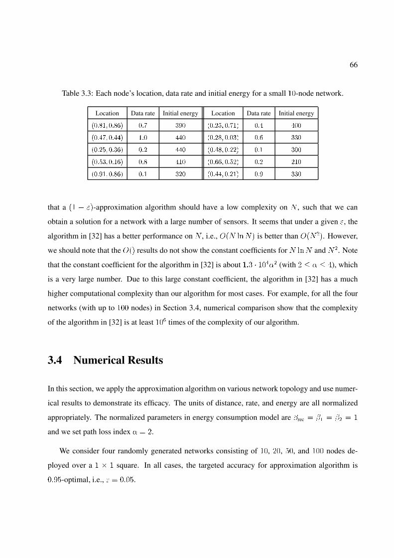
66

Table 3.3: Each node’s location, data rate and initial energy for a small ��-node network.

Location Data rate Initial energy Location Data rate Initial energy

��#�� #�� #� �� #�� #�� #� ��

��#�� #�� #� �� #�� #�� #� ��

��#�� #�� # �� #�� #� �#� ��

��#�� #�� #� �� #�� #�� # ��

��#�� #�� #� �� #�� #�� #� ��

that a �� -approximation algorithm should have a low complexity on � , such that we can

obtain a solution for a network with a large number of sensors. It seems that under a given �, the

algorithm in [32] has a better performance on � , i.e., #�� is better than #��. However,

we should note that the #�� results do not show the constant coefficients for � �� and ��. Note

that the constant coefficient for the algorithm in [32] is about �� (with � � � � �), which

is a very large number. Due to this large constant coefficient, the algorithm in [32] has a much

higher computational complexity than our algorithm for most cases. For example, for all the four

networks (with up to �� nodes) in Section 3.4, numerical comparison show that the complexity

of the algorithm in [32] is at least �� times of the complexity of our algorithm.

3.4 Numerical Results

In this section, we apply the approximation algorithm on various network topology and use numer-

ical results to demonstrate its efficacy. The units of distance, rate, and energy are all normalized

appropriately. The normalized parameters in energy consumption model are rec � � � � � �

and we set path loss index � � �.

We consider four randomly generated networks consisting of ��, ��, ��, and �� nodes de-

ployed over a � � � square. In all cases, the targeted accuracy for approximation algorithm is

��-optimal, i.e., � � ��.

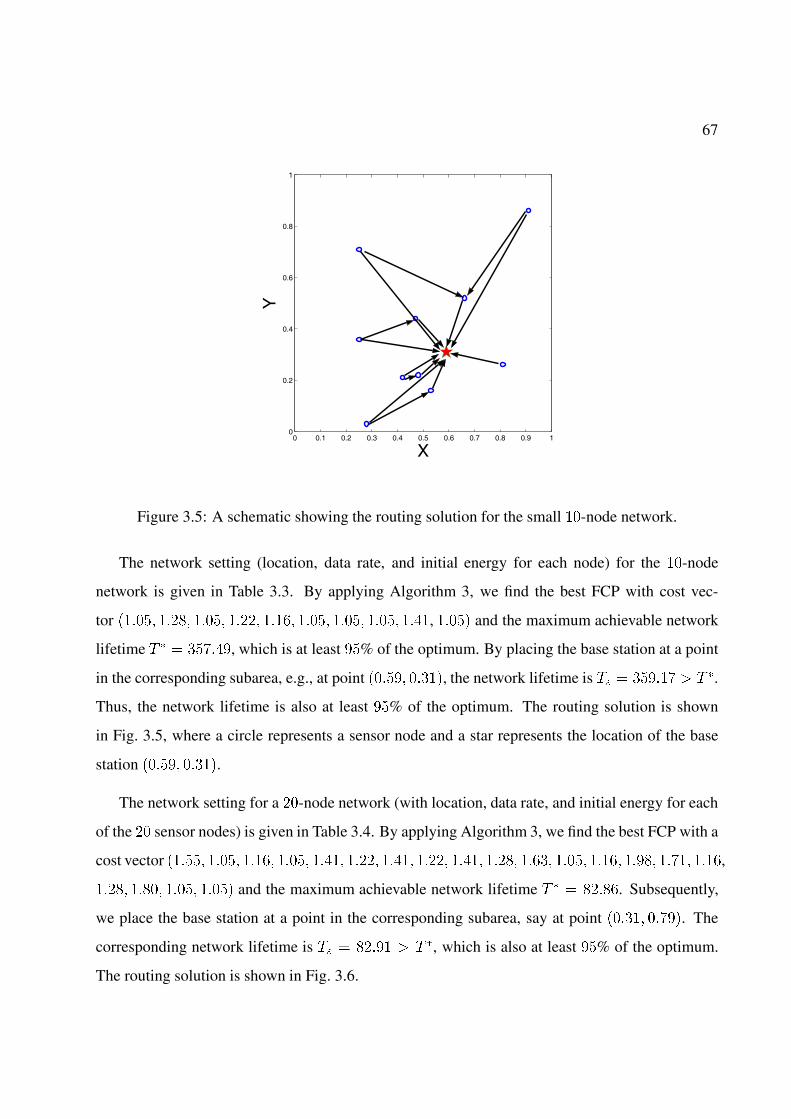
67

0 0.1 0.2 0.3 0.4 0.5 0.6 0.7 0.8 0.9 10

0.2

0.4

0.6

0.8

1

X

Y

Figure 3.5: A schematic showing the routing solution for the small ��-node network.

The network setting (location, data rate, and initial energy for each node) for the ��-node

network is given in Table 3.3. By applying Algorithm 3, we find the best FCP with cost vec-

tor �� , �� and the maximum achievable network

lifetime � � ��, which is at least ��% of the optimum. By placing the base station at a point

in the corresponding subarea, e.g., at point �� , the network lifetime is �� .

Thus, the network lifetime is also at least ��% of the optimum. The routing solution is shown

in Fig. 3.5, where a circle represents a sensor node and a star represents the location of the base

station �� .

The network setting for a ��-node network (with location, data rate, and initial energy for each

of the �� sensor nodes) is given in Table 3.4. By applying Algorithm 3, we find the best FCP with a

cost vector �� ,

�� and the maximum achievable network lifetime � � ��. Subsequently,

we place the base station at a point in the corresponding subarea, say at point �� . The

corresponding network lifetime is �� , which is also at least ��% of the optimum.

The routing solution is shown in Fig. 3.6.

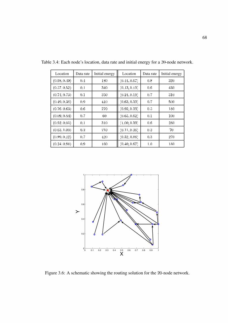
68

Table 3.4: Each node’s location, data rate and initial energy for a ��-node network.


��#�� #�� #� �� #�� #�� #� ��

��#�� #�� #� �� #�� #�� #� ��

��#�� #�� #� �� #�� #�� #� ��

��#�� #�� #� �� #�� #�� #� ��

��#�� #�� #� �� #�� #�� #� ��

��#�� #�� #� �� #�� #�� #� ��

��#�� #�� #� �� #�� #�� #� ��

��#�� #�� # �� #�� #�� #� ��

��#�� #�� #� �� #�� #�� #� ��

��#�� #�� #� �� #�� #�� #� ��

0 0.1 0.2 0.3 0.4 0.5 0.6 0.7 0.8 0.9 10

0.2

0.4

0.6

0.8

1

X

Y

Figure 3.6: A schematic showing the routing solution for the ��-node network.

69

0 0.1 0.2 0.3 0.4 0.5 0.6 0.7 0.8 0.9 10

0.2

0.4

0.6

0.8

1

X

Y

(a) A ��-node network.

0 0.1 0.2 0.3 0.4 0.5 0.6 0.7 0.8 0.9 10

0.2

0.4

0.6

0.8

1

X

Y

(b) A ��-node network.

Figure 3.7: Network topology for ��-node and ��-node networks.

For the ��-node and ��-node networks, the positions of the nodes and location for the base

station are shown in Fig. 3.7(a) and (b), respectively. The data rate and initial energy for each node

are randomly generated between �� and �� , respectively. For the 50-node network, we

obtain a �� -optimal solution with �� when the base station is placed at �� ;

for the 100-node network, the �� -optimal solution is �� when the base station is

placed at �� .

We now compare the complexity of our algorithm with the approximation algorithm proposed

in [32] for the ��, ��, ��, and ��-node network considered in this section. Corresponding to each

network topology, based on (3.9) and (3.10), we find that the complexity of the approximation

algorithm in [32] is �� , �� , �� , and �� times of the complexity of our

approximation algorithm.

70

3.5 Related Work

Due to energy constraint, network lifetime for a wireless sensor network is limited. As a re-

sult, there is a flourish of research activities in this area in recent years. Many of these efforts

(e.g., [11,15,55,111]) studied lifetime problem under given network topology and without explicit

consideration on the impact of node placement on network performance.

Among the body research on node placement, researchers have studied sensor node place-

ment [29, 103, 107, 114], relay node placement [49, 109], and base station placement [14, 32, 73].

The main focus of sensor node placement has been on coverage in order to have either better

geographical coverage of the area or better connectivity in the network. Relay node placement

deals with how to place special auxiliary nodes within a sensor network so that network per-

formance (e.g., connectivity, lifetime) can be improved. Related work in relay node placement

(e.g., [49,109]) have been limited to heuristic algorithm instead of providing performance guaran-

tee.

Related work on base station placement include [14, 32, 73]. In [14], Bogdanov et al. studied

how to place base station so that the network flow is proportionally maximized subject to link

capacity. The authors show that although it is possible to find optimal solutions for special network

topology (e.g., grid), the base station placement problem for an arbitrary network is NP-complete.

The authors also pointed out that an approximation algorithm with any guarantee was not known

at the time of their paper and subsequently proposed two heuristic algorithms. In [73], Pan et al.

studied base station placement problem to maximize network lifetime. The optimal location is

only determined for the simple case where only single-hop routing is allowed. The more difficult

problem involving multi-hop routing was not addressed.

In [32], Efrat et al. proposed the first �� -optimal approximation algorithm to the base

station placement problem. However, since they constructed a finite search space of physical

points, the computational complexity of their algorithm is higher than the one proposed in this

chapter for most cases, as illustrated in Section 3.3.4.

71

3.6 Conclusions

In this chapter, we investigated the base station placement problem for a multi-hop sensor network.

The main result is an approximation algorithm that can guarantee �� -optimal network lifetime

performance for base station placement problem with any desired error bound � � �. The proposed

�� -approximation algorithm was based on several novel techniques such as discretization

of cost parameters (and distances), division of search space into finite number of subareas, and

representation of subareas with fictitious cost points (with nice bounding properties on costs).

We gave a proof that the proposed approximation algorithm is �� -optimal. The proposed

approximation algorithm offers significant complexity reduction when compared to a state-of-the-

art algorithm and represents the best known result to the described base station placement problem.

Chapter 4

Mobile Base Station for Wireless Sensor

Networks

4.1 Introduction

The benefits of using mobile base station to prolong sensor network lifetime have been well rec-

ognized [62, 110]. Since base station is the sink node for data generated by all the sensor nodes in

the network, this approach aims to alleviate the traffic aggregation burden from a fix set of sensor

nodes near the base station to other sensor nodes in the network, and it is possible to extend the

network lifetime significantly.

Indeed, although the practical feasibility of using a mobile base station is still considered far-

fetched a few years ago, such capabilities are nowadays reality, thanks to recent breakthrough in

unmanned autonomous vehicle (UAV) competition by DARPA’s Grand Challenge program [24]

and advances in customized robotics for sensors [91]. It has now become entirely plausible to

consider that an unmanned vehicle be employed to serve as a mobile base station for sensor data

collection.

Although the potential benefit of using mobile base station to prolong sensor network lifetime

72

73

is significant, the theoretical difficulty of this problem is enormous. There are two components

that are tightly coupled in this problem. First, the location of the base station is now a function of

time, i.e., at different time instances, we have a different physical network topology, with the sink

node being at different positions. Second, the traffic (or flow) routing behavior may change with

both time as well as the location of the base station. As a result, an optimization problem with the

objective of maximizing the network lifetime needs to consider both base station location (time-

dependent) and flow routing. Due to these difficulties, existing solutions to this problem remain

heuristic at best (e.g., [62, 110]) and cannot provide provably optimal solution to network lifetime

performance.

To fill in this theoretical gap, this chapter offers an in-depth study on the network lifetime

performance limit when mobile base station is employed. We formulate an optimization problem

with base station movement and flow routing as part of the constraints. As a first step, we show

that as far as network lifetime objective is concerned, flow routing only needs to be dependent on

the base station location, regardless of when the base station is present at this location. Further,

the specific time instances for the base station to visit a location is not important, as long as the

total sojourn time for the base station to be present at this location is fixed. With this finding, we

show how to make a novel transformation from a time-dependent problem formulation to location

(space)-dependent problem formulation.

As a second step, we show that when base station is only allowed to be present at a finite

set of pre-determined points (called constrained mobile base station (C-MB) problem), we can

find the optimal sojourn time for the base station to stay on each of these points (as well as the

corresponding flow routing solution) such that the overall network lifetime (i.e., sum of the sojourn

times) is maximized via a single linear program (LP).

Building upon these results, the main result in this chapter (Section 4.5) shows that for the un-

constrained mobile base station (U-MB) problem, i.e., the base station can be present at any point

in the two dimensional plane, we can develop a provably �� -optimal algorithm that provides a

solution with network lifetime guaranteed to be at least �� of the maximum network lifetime

74

(albeit it is unknown), where � can be made arbitrarily small depending on required precision. The

main idea in this approximation algorithm is to exploit a clever way of dividing the search space

into subareas, with each of its link cost having some nice properties that are related to �� -

optimal. A novel idea in the design of �� -optimal algorithm is to represent each subarea with

so-called “fictitious cost point,” which is an � -tuple cost vector with each component representing

an upper bound of cost to the respective node. As a result, we can apply the LP approach developed

for the C-MB problem on the fictitious cost points and develop provably �� -optimal solution.

The remainder of this chapter is organized as follows. In Section 4.2, we describe the network

model and introduce the mobile base station problem. In Section 4.3, we present a novel trans-

formation that enables to transform a time-dependent problem to a space-dependent problem. In

Section 4.4, we develop optimal solution for the constrained mobile base station (C-MB) problem.

Section 4.5 presents the main result of this chapter, which is an algorithm for the unconstrained

mobile base station (U-MB) problem with provably �� -optimal network lifetime. Section 4.6

reviews related work and Section 4.7 concludes this chapter.

4.2 Network Model and Problem Formulation

4.2.1 Network Model

We consider a set � of nodes deployed over a two-dimensional area, with the location of each

sensor node � being at a point �� )��. We assume each node generates data at a rate of ��.

There is a base station ( for the sensor network and it serves as the sink node for all data. Data

generated by each sensor node can be transmitted via single or multi-hop toward the base station.

Each node � is initially provisioned with an amount of energy ��. The base station is

not constrained with energy. In this study, network lifetime is defined as the first time instance

when any of the sensor nodes runs out of energy. Power consumption model has been discussed

in Section 2.2.2. From (2.1), (2.2), and (2.3), it is easy to understand that the location of the base

75


�� Flow rate from node � to node � when base station � is at point �

�� Flow rate from node � to node � at time �

�C-MB The maximum network lifetime achieved by ��C-MB

U-MB �� -optimal network lifetime achieved by �U-MB

$ �� Sojourn time for the base station to be present at point �

$ �%�� Sojourn time for the base station to be present in subarea %�

�&� '�� Location of base station � at time �

�&�� '�� Location of sensor node �

�� Cost for transmitting data from sensor � to base station � at time �

�� Cost for transmitting data from sensor node � to base station � when � is at point �

��C-MB An optimal solution to the C-MB problem

�U-MB �� -optimal solution to the U-MB problem

station and the corresponding flow routing among the nodes will determine energy consumption

behavior at each node and thus the network lifetime. Table 4.1 lists all notation that are used only

in this chapter.

4.2.2 Problem Description

The focus of this chapter is to investigate how to optimally move a mobile base station to collect

real time data in a sensor network so that the network lifetime can be maximized. Note that the

network lifetime problem has attracted great interest even for static (fixed) base station problem

(e.g., [15, 17, 18, 87]).

As a first step, we consider the case when the base station is only allowed to be present at a

set of pre-determined * positions, denoted as �� . We call this problem as constrained

mobile base station (C-MB) problem. Results on C-MB problem will help us devise solution to

the general problem where the base station is allowed to roam anywhere on the two-dimensional

plane. We term the latter problem unconstrained mobile base station (U-MB) problem.

76

Denote �� )�� the position of base station ( at time � and � the network lifetime (which is

an optimization variable). Then a feasible flow routing solution realizing this network lifetime �

must satisfy both flow balance and energy constraints at each sensor node. These constraints can

be formally stated as follows. Denote �� and �� the data rates from node to node ' and

base station ( at time �, respectively. Then the flow balance for each sensor node � at any

time � �� is� ��

��

��

��

i.e., the sum of total incoming flow rates plus self-generated data rate is equal to the sum of total

outgoing flow rates at time � �� . The energy constraint for each sensor node � is

� �

�

��

�rec��

��

��

��

i.e., total consumed energy due to reception and transmission over time � cannot exceed its initial

energy ��. By (2.2), we have

��

�� )�� )��

��

Denote � the search space for the base station, which can be narrowed down to the smallest

enclosing disk for all nodes in the network (see Lemma 3). The general U-MB problem can be

formulated as follows.

Max �

s.t.��

��

��

�

�� rec��

� ��

��

��

�� )�� )��

��

�� )��

�� ' � � ��'� ��

In the above formulation, the base station location (i.e., �� )�� for � � � � � ) and the

corresponding flow routing (i.e., �� and �� for � � � � � ) form a joint optimization space

77

for the objective � . This formulation is in the form of non-polynomial program. Since even a

simpler non-linear programming problem is NP-hard in general [40], we conclude that the above

formulation is also NP-hard in general.

4.3 From Time Domain to Space Domain

The difficulty of the formulated problem in last section resides in that base station location �� )��

and flow routing �� and �� are all functions of time. In this section, we show that as far as

network lifetime performance is concerned, such dependency on time can be relaxed. Specifically,

we will show (Theorem 4) that the flow routing only needs to be dependent on the location of the

base station and independent of when the base station is present at this location. Further, as long

as the total sojourn time for this location is the same, “when” the base station visits this location is

not important.

To start with, we define the indicator function ��event� as � if event is true and � otherwise.

Denote 0 �� the cumulative time periods for the base station ( to be present at location under

a solution �, i.e.,

0 ��

� �

�

�� )�� (4.1)

We have the following theorem.

Theorem 4. Denote � the maximum network lifetime achieved by an optimal solution � with a

base station moving path �� )�� and a flow routing �� and ��. There exists an equivalent

solution � with 0 �� and time-independent flow rates � �� and � �� that yields the same

maximum network lifetime. Under � �� and � ��, as long as 0 �� remain the same, the

network lifetime � will remain unchanged regardless of the specific time instances when the base

station visits each point .

The proof of Theorem 4 is based on the Lemmas 5 and 6.

78

Lemma 5. Given a feasible solution � with a specific base station moving path �� )��, a time-

varying flow routing �� and ��, and a corresponding network lifetime � , we can find a

solution � with location-dependent flow rates �� and �� for each point in path �� )��

that yields the same network lifetime � by having the base station following the same moving path

and setting the flow routing on any point in this path as

��

�

�� )��

0 ��

��

�

��

�� )��

0 ��

In essence, Lemma 5 focus on flow routing component and shifts the flow routing’s dependency

from time domain to space domain. We use the following simple example to illustrate this idea.

Example 1. For illustration purpose, we consider a simple -node sensor network shown in

Fig. 4.1. Each node generates data at a bit rate of �. We assume all units are normalized ap-

propriately. The network lifetime is �� under a solution �, where the base station stays at �

during periods �� and �� , and stays at � during �� . The flow routing for each

period is given in Fig. 4.1(a)–(d), with bit rate of each flow marked on the respective flow arrow.

Note that the flow routing for periods �� and �� are different, despite that the base

station is located at � during both periods. Further, during �� , the flow routing changes

between periods �� and �� while the base station is at �.

Under �, we show that as far as achieving the same network lifetime, flow routing only needs

to be dependent on the base station’s location. For example, under �, the total time that the base

station stays at � is �� (� �� ). During the time periods when the base station is at �,

�� when � � � � �� and �� when �� . Thus, the average

rate on link � ( when the base station stays at � is �� ,�� . We

can set �� under �. Similarly, we obtain the average rate �� and

�� , respectively. This lead to a new flow routing shown in Fig. 4.2(a) for periods

�� and �� . Following the same token, we can convert the flow routing in Fig. 4.1(b) and

(c) to that in Fig. 4.2(b), i.e., �� , �� , �� , and �� .

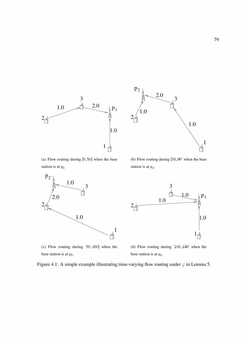
79

1.0

1.0

1

3

2

p12.0

(a) Flow routing during �� when the base

station is at ��.

2

1.0

1.0

2.0

2

1

3

p

(b) Flow routing during �� when the base

station is at ��.

2

1.0

1.0

2.02

1

3

p

(c) Flow routing during �� when the

base station is at ��.

1.0

1

3

1

2

p

1.0

1.0

(d) Flow routing during �� when the


Figure 4.1: A simple example illustrating time-varying flow routing under � in Lemma 5.

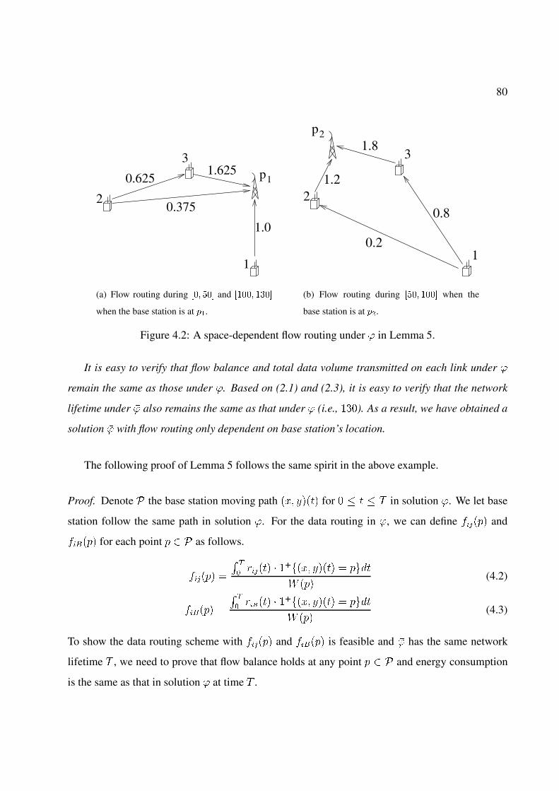
80

0.625

0.375

1

3

2

p1

1.0

1.625

(a) Flow routing during �� and ��

when the base station is at ��.

0.2

0.8

1.8

1.22

1

3

p2

(b) Flow routing during �� when the


Figure 4.2: A space-dependent flow routing under � in Lemma 5.

It is easy to verify that flow balance and total data volume transmitted on each link under �

remain the same as those under �. Based on (2.1) and (2.3), it is easy to verify that the network

lifetime under � also remains the same as that under � (i.e., ��). As a result, we have obtained a

solution � with flow routing only dependent on base station’s location.

The following proof of Lemma 5 follows the same spirit in the above example.

Proof. Denote � the base station moving path �� )�� for � � � � � in solution �. We let base

station follow the same path in solution �. For the data routing in �, we can define �� and

�� for each point � as follows.

��

�

��

�� )��

0 ��(4.2)

��

�

�� )��

0 ��(4.3)

To show the data routing scheme with �� and �� is feasible and � has the same network

lifetime � , we need to prove that flow balance holds at any point � and energy consumption

is the same as that in solution � at time � .

81

For flow balance when base station is at any point � , we have

� ��

��

� ��

�

�� )��

0 ��

�

�� )��

0 ��

�

�

�

��

� �� )��

0 ��

�

�

�

��

� �� )��

0 ��

�

��

�

�� )��

0 ��

�

�� )��

0 ��

�

��

��

The first equality holds by (4.2). The third equality holds by the flow balance in solution �. The

last equality holds by (4.2) and (4.3).

For energy consumption at time � , we first have�

� �

�

�� )��

�

�

��

� �

�

�� )��

�

�

��

�

��

�� )��

0 ��

� �

�

�� )��

�

�

��

� �

�

�� )��

�

�

� �

�

�� )��

�

�

� �

�

�� )��

�

� �

�

�� (4.4)

for any node � . The second equality holds by (4.3). The third equality holds by (4.1).

Similarly, we have �

� �

�

�� )��

� �

�

�� (4.5)

82

for any � ' � � �� '. Thus, we have

�

� �

�

��

rec��

��

��

� �� )��

�

� ��

rec

�

� �

�

�� )��

��

�

�

� �

�

�� )��

�

�

� �

�

�� )��

�

� ��

� �

�

rec��

��

� �

�

��

� �

�

��

The second equality holds by (4.4) and (4.5). The last inequality holds due to the energy constraint

under �. Thus, the data routing with �� and �� is feasible and has the same network lifetime

� . This completes the proof.

The following lemma further extends Lemma 5 and says that the specific time instances for the

base station to visit a particular point is not important. As long as 0 �� remain the same, the

network lifetime remains unchanged. For example, in the transformed solution � in Fig. 4.2, as

long as the base station stays at point � for a time period of �� (� �� ) and point � for a

time period of ��, the exact time instances when the base station is present at this location is not

important in terms of achieving the same network lifetime.

Lemma 6. Given a feasible solution � with a base station moving path �� )��, a flow routing

�� and ��, and a network lifetime � , we can compute 0 �� by (4.1) and define base station

location-dependent flow routing �� and �� as in Lemma 5. Under �� and ��, as

long as 0 �� remain the same, the network lifetime � will remain unchanged regardless of the

ordering and frequency of the base station’s presence at each point .

Lemma 6 can be easily proved by analyzing the energy consumption behavior at each node

over time � . We omit its proof here. Combining Lemmas 5 and 6 and considering the special case

that � is optimal, we have Theorem 4.

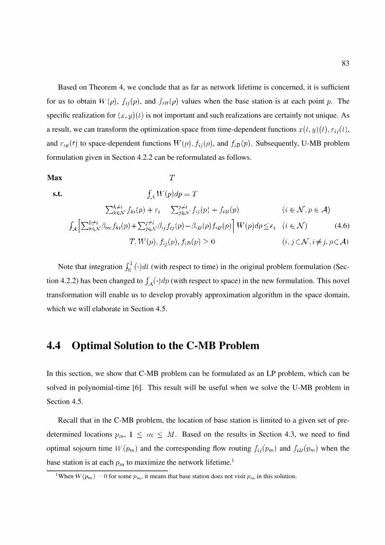
83

Based on Theorem 4, we conclude that as far as network lifetime is concerned, it is sufficient

for us to obtain 0 ��, ��, and �� values when the base station is at each point . The

specific realization for �� )�� is not important and such realizations are certainly not unique. As

a result, we can transform the optimization space from time-dependent functions �� )�� ,

and �� to space-dependent functions 0 �� , and ��. Subsequently, U-MB problem

formulation given in Section 4.2.2 can be reformulated as follows.

Max �

s.t.�0 ��

��

��

�� rec��

� ��

0 �� (4.6)

��0 �� '� � ��'� ��

Note that integration �

�� (with respect to time) in the original problem formulation (Sec-

tion 4.2.2) has been changed to�� (with respect to space) in the new formulation. This novel

transformation will enable us to develop provably approximation algorithm in the space domain,

which we will elaborate in Section 4.5.

4.4 Optimal Solution to the C-MB Problem

In this section, we show that C-MB problem can be formulated as an LP problem, which can be

solved in polynomial-time [6]. This result will be useful when we solve the U-MB problem in

Section 4.5.

Recall that in the C-MB problem, the location of base station is limited to a given set of pre-

determined locations �, � � ! � * . Based on the results in Section 4.3, we need to find

optimal sojourn time 0 �� and the corresponding flow routing �� and �� when the

base station is at each � to maximize the network lifetime.1

1When $ �� for some ��, it means that base station does not visit �� in this solution.

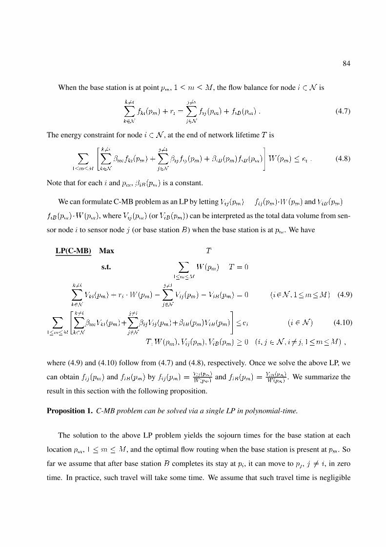
84

When the base station is at point �, � � ! � * , the flow balance for node � is

� ��

��

��

�� (4.7)

The energy constraint for node � , at the end of network lifetime � is

��

��

rec��

��

��

0 �� (4.8)

Note that for each and �, �� is a constant.

We can formulate C-MB problem as an LP by letting �� 0 �� and ��

�� 0 ��, where �� (or ��) can be interpreted as the total data volume from sen-

sor node to sensor node ' (or base station () when the base station is at �. We have

LP(C-MB) Max �

s.t.�

��

0 ��

� ��

�� 0 ��

��

�� !�*� (4.9)

��

��

rec��

��

��

�� (4.10)

��0 �� ' � � ��'� ��!�*� �

where (4.9) and (4.10) follow from (4.7) and (4.8), respectively. Once we solve the above LP, we

can obtain �� and �� by ��

� ��and ��

��

. We summarize the

result in this section with the following proposition.

Proposition 1. C-MB problem can be solved via a single LP in polynomial-time.

The solution to the above LP problem yields the sojourn times for the base station at each

location �, � � ! � * , and the optimal flow routing when the base station is present at �. So

far we assume that after base station ( completes its stay at �, it can move to , ' �� , in zero

time. In practice, such travel will take some time. We assume that such travel time is negligible

85

comparing with the time scale of network lifetime (typically several months). It can be shown that

if buffering is available at sensor node, the maximum network lifetime can still be achieved. In

this case, each node needs to slightly delay its transmission until the base station arrives at its new

location.

4.5 An Approximation Algorithm to the U-MB Problem

Building upon the results in the previous sections, we are now ready to present the main result of

this chapter.

4.5.1 Subareas and Fictitious Cost Points

Under the U-MB problem, the base station can move to any point in the two-dimensional plane.

Clearly, in order to maximize network lifetime, we would expect that the location for the base

station can be narrowed down to the smallest enclosing disk (SED) [106]. The proof is similar to

that for Lemma 3.

Although we have narrowed down the search space for base station ( from an infinite two-

dimensional plane to SED �, there still exist infinite number of points in �. To obtain a finite

search space, we follow the same approach in Section 3.3.2 to divide SED into subareas and to

represent each subarea by a fictitious cost point (FCP).

Suppose we have the set of * non-uniform subareas that are represented by * FCPs. We now

readily apply the LP approach discussed in Section 4.4 to formulate an optimization problem on

these * FCPs. In next section, we will show that an optimal solution to the C-MB problem on

FCPs can be used to construct a �� -optimal solution to the U-MB problem.

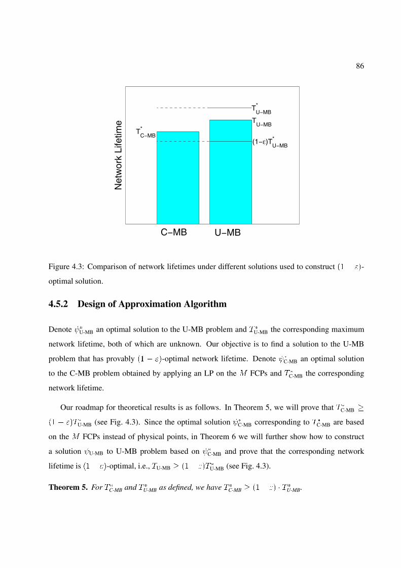
86

Net

wor

k Li

fetim

e

C−MB U−MB

TC−MB*

TU−MB

TU−MB*

(1−ε)TU−MB*

Figure 4.3: Comparison of network lifetimes under different solutions used to construct �� -

optimal solution.

4.5.2 Design of Approximation Algorithm

Denote -U-MB an optimal solution to the U-MB problem and � U-MB the corresponding maximum

network lifetime, both of which are unknown. Our objective is to find a solution to the U-MB

problem that has provably �� -optimal network lifetime. Denote -C-MB an optimal solution

to the C-MB problem obtained by applying an LP on the * FCPs and � C-MB the corresponding

network lifetime.

Our roadmap for theoretical results is as follows. In Theorem 5, we will prove that � C-MB

�� U-MB (see Fig. 4.3). Since the optimal solution -C-MB corresponding to � C-MB are based

on the * FCPs instead of physical points, in Theorem 6 we will further show how to construct

a solution -U-MB to U-MB problem based on -C-MB and prove that the corresponding network

lifetime is �� -optimal, i.e., �U-MB �� U-MB (see Fig. 4.3).

Theorem 5. For � C-MB and � U-MB as defined, we have � C-MB �� U-MB.

87

To prove that Theorem 5 is true, we need the following lemma, where subareas �� and FCPs

�, � � ! � * are defined the same as in Section 3.3.2 for a given � � �. Denote 0 ��

the cumulative time period when the base station ( is present within subarea �� for the U-MB

problem. We have

0 ��

��

0 �� (4.11)

Lemma 7. Suppose we have a given solution �U-MB to the U-MB problem with 0 ��, ��,

��, and a network lifetime �U-MB. For a given � � �, we can always construct a solution �C-MB

to C-MB problem on these FCPs such that network lifetime �C-MB �� U-MB by having the

base station spend 0 �� amount of time on FCP �, where

0 �� 0 �� (4.12)

and setting the flow routing on � as

��

��

��0 ��

0 �� (4.13)

��

��

��0 ��

0 �� (4.14)

Proof. We will show solution �C-MB is feasible, i.e., flow balance holds at each point, and the

network lifetime of �C-MB is at least �� U-MB.

For flow balance when the base station location is �, we have� ��

��

� ��

��

��0 ��

0 ��

��

��0 ��

0 ��

�

��

��

0 ��

0 ��

�

��

��

0 ��

0 ��

�

��

��

��

0 ��

��

��

0 ��

�

��

��

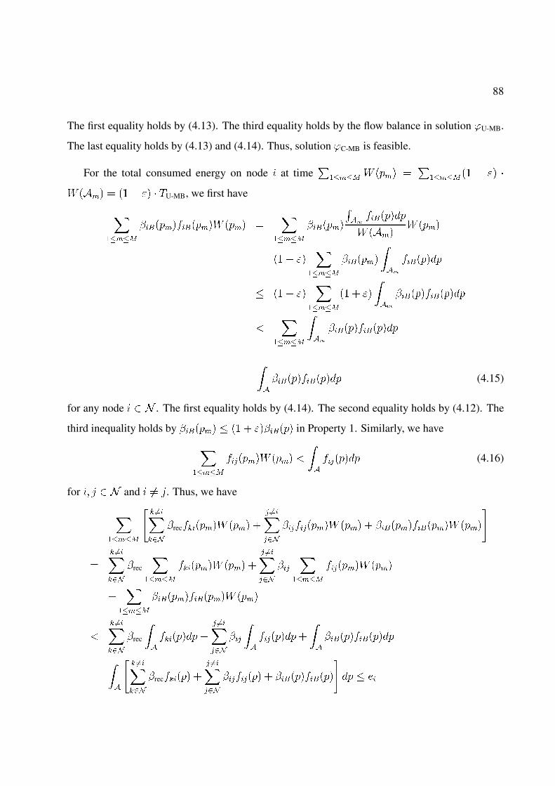
88

The first equality holds by (4.13). The third equality holds by the flow balance in solution �U-MB.

The last equality holds by (4.13) and (4.14). Thus, solution �C-MB is feasible.

For the total consumed energy on node at time�

�� 0 ��

��

0 �� U-MB, we first have

��

��0 ��

��

��

��

��

0 ��0 ��

� ��

��

��

��

��

� ��

��

��

��

��

��

��

��

��

�

��

�� (4.15)

for any node � . The first equality holds by (4.14). The second equality holds by (4.12). The

third inequality holds by �� in Property 1. Similarly, we have

��

��0 ��

��

�� (4.16)

for � ' � and �� '. Thus, we have

��

��

rec��0 ��

��

��0 �� 0 ��

�

� ��

rec

��

��0 ��

��

��

��

��0 ��

��

��

��0 ��

�

� ��

rec

��

��

��

�

��

��

��

��

�

��

��

rec��

��

��

� � ��

89

The first equality holds by (4.15) and (4.16). The last inequality holds by the energy constraint

in solution �U-MB. Thus, the network lifetime of solution �C-MB is at least �� U-MB. This

completes the proof.

Lemma 7 is a powerful result. It states that for any given solution �U-MB to the U-MB problem,

we can find a solution �C-MB for the set of FCPs (corresponding to a given �), such that the network

lifetime �C-MB is at least �� of �U-MB.

Now we are ready to prove Theorem 5.

Proof. Considering the special case of Lemma 7 that the given solution to U-MB problem is an

optimal solution with network lifetime � U-MB, we can transform it into a solution to C-MB problem

on FCPs with network lifetime at least �� U-MB, i.e., there is a solution to C-MB problem on

FCPs with network lifetime of at least �� U-MB. Thus, the solution -C-MB to C-MB problem

on FCPs must have a network lifetime � C-MB �� U-MB.

Theorem 5 guarantees that the network lifetime obtained from the LP solution on the * FCPs

is at least �� of � U-MB. As discussed in Section 3.3.2, the � -tuple vector embodied by an

FCP only represents the upper cost bound for any point in the corresponding subarea to the �

nodes in the network and an FCP may not be mapped to a physical point, which is required in the

final solution. In the following theorem, we show that if we have an optimal solution to the C-MB

problem based on FCPs, we can construct a solution with each point being physically realizable.

Further, the network lifetime for this constructed solution is greater than or equal to the maximum

network lifetime for the C-MB problem, i.e., �U-MB � C-MB. As a result, this new solution is

�� -optimal.

Theorem 6. For a given � � �, define subareas �� and FCPs �, � � ! � * , as discussed in

Section 3.3.2. Obtain an optimal solution -C-MB on these * FCPs with 0 ��, � ��, ��,

and corresponding network lifetime � C-MB as discussed in Section 4.4. A �� -optimal solution

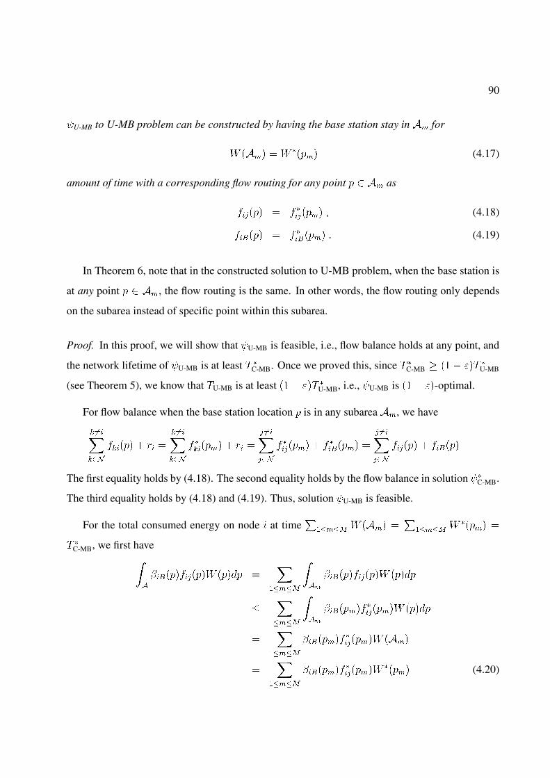
90

-U-MB to U-MB problem can be constructed by having the base station stay in �� for

0 �� 0 �� (4.17)

amount of time with a corresponding flow routing for any point �� as

�� (4.18)

�� (4.19)

In Theorem 6, note that in the constructed solution to U-MB problem, when the base station is

at any point ��, the flow routing is the same. In other words, the flow routing only depends

on the subarea instead of specific point within this subarea.

Proof. In this proof, we will show that -U-MB is feasible, i.e., flow balance holds at any point, and

the network lifetime of -U-MB is at least � C-MB. Once we proved this, since � C-MB �� U-MB

(see Theorem 5), we know that �U-MB is at least �� U-MB, i.e., -U-MB is �� -optimal.

For flow balance when the base station location is in any subarea ��, we have

� ��

��

� ��

� ��

��

� ��

��

��

The first equality holds by (4.18). The second equality holds by the flow balance in solution -C-MB.

The third equality holds by (4.18) and (4.19). Thus, solution -U-MB is feasible.

For the total consumed energy on node at time�

�� 0 ��

�� 0 ��

� C-MB, we first have��

��0 ��

��

��

��0 ��

��

��

��

��0 ��

��

��

��0 ��

��

��

��0

�� (4.20)

91

for any node � . The second inequality holds by (4.19) and �� in Property 1.

The third equality holds by (4.11). The last equality holds by (4.17). Similarly, we have��

��0 ��

��

� ��0�� (4.21)

for � ' � and �� '. Thus, we have

��

��

rec��0 ��

��

��0 �� 0 ��

�

�

� ��

rec

��

��0 ��

��

�

��

��0 ��

��

��0 ��

�

� ��

rec

��

� ��0��

��

��

��

� ��0��

��

��

��0

��

� ��

The first equality holds by (4.20) and (4.21). The second equality holds by the energy constraint

in solution -C-MB. Thus, the network lifetime of solution -U-MB is at least � C-MB �� U-MB.

This completes the proof.

4.5.3 Summary of Algorithm and Example

The design of the �� -optimal algorithm are given in Sections 4.5.1 and 4.5.2. We now sum-

marize it into the following algorithm.

Algorithm 4. (A �� -Optimal Algorithm)

1. Narrow down the search space for base station within smallest enclosing disk �.

2. Within the smallest enclosing disk �, compute the lower and upper cost bounds min�� and

max�� for each node � by (3.3) and (3.4).

92

Table 4.2: Sensor locations, data rate, and initial energy of the example sensor network

Node Index Location Data rate Initial energy

1 ��#�� #�� #� ��

2 ��#�� #�� #� ��

3 ��#�� #�� #� ��

3. For a given � � �, define a sequence of costs ��, �� +�� by (3.5), where +� is

defined by (3.6).

4. For each node � , draw a sequence of �+�� circles corresponding to cost �� centered

at node , � � � � +�. The intersection of these circles within disk � will divide � into *

subareas ��, �� .

5. For each subarea��, � � ! � * , define an FCP �, which is represented by � -tuple cost

vector �� , where �� is defined in (3.8).

6. For the C-MB problem on these * FCPs, apply the LP formulation in Section 4.4 and obtain

an optimal solution -C-MB with 0 ��, � ��, and � ��.

7. Construct a �� -optimal solution -U-MB to U-MB problem based on -C-MB using the

procedure in Theorem 6.

In the above algorithm, Step 6 has the highest complexity (solving an LP). By (3.9), the total

number of subareas * is upper bounded by #��,��. Thus, the LP in Step 6 has polynomial

size and the complexity of the above algorithm is polynomial.

Example 2. To illustrate the steps in Algorithm 4, we solve a small -sensor network problem as

an example. The location, data rate, and initial energy for each sensor are shown in Table 4.2,

where the units of distance, rate, and energy are all normalized. We use � � � in this example and

the network setting are � � �, � � �� and rec � � under normalized units. For illustration, we

93

2

3

4

5

6

7

9

10

11

12

13

14

15

16

17

0 0.2 0.4 0.6X

0.8 1

0

0.2

0.4

0.6

0.8

1

Y

81

Figure 4.4: The subareas for the example sensor network.

set � � ��.2

In Step 1, we identify SED � with origin #� � �� and radius �� (see

Fig. 4.4).

In Step 2, We have 1�� for each node , � � � . We then find the lower and

upper bounds of �� for each node as follows.

min��

max�� 1��

� � � � ��

In Step 3, for � � ��, we find

+� �

��

��1��

��

��

��

��

��

��

��

2In Section 4.5.4, we use � � �#�� for all numerical results.

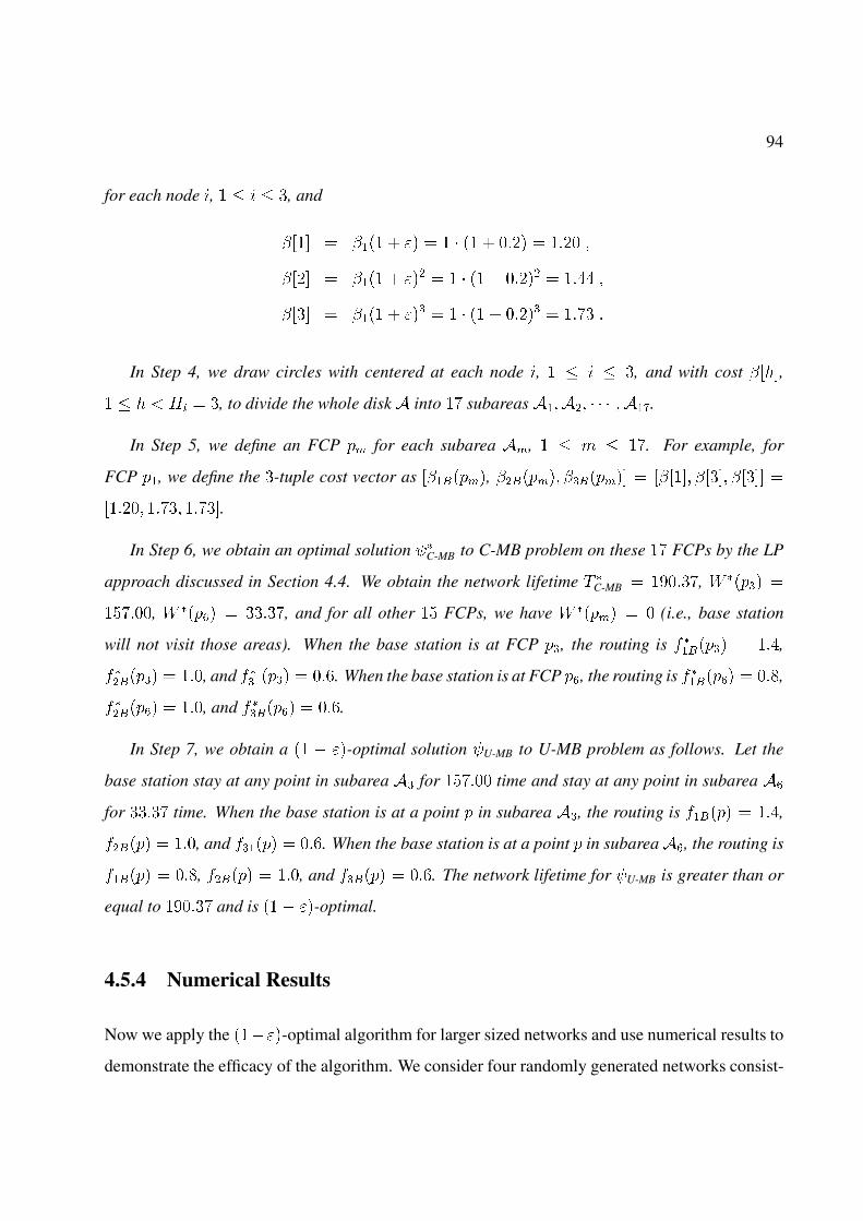
94

for each node , � � � , and

��

��

� � ��

In Step 4, we draw circles with centered at each node , � � � , and with cost ��,

� � � � +� � , to divide the whole disk � into �� subareas �� .

In Step 5, we define an FCP � for each subarea ��, � � ! � ��. For example, for

FCP �, we define the -tuple cost vector as ��, ��

�� .

In Step 6, we obtain an optimal solution -C-MB to C-MB problem on these �� FCPs by the LP

approach discussed in Section 4.4. We obtain the network lifetime � C-MB � ��, 0 ��

��, 0 �� , and for all other �� FCPs, we have 0 �� (i.e., base station

will not visit those areas). When the base station is at FCP , the routing is � �� ,

� �� , and � �� . When the base station is at FCP �, the routing is � �� ,

� �� , and � �� .

In Step 7, we obtain a �� -optimal solution -U-MB to U-MB problem as follows. Let the

base station stay at any point in subarea � for �� time and stay at any point in subarea ��

for �� time. When the base station is at a point in subarea �, the routing is �� ,

�� , and �� . When the base station is at a point in subarea��, the routing is

�� , �� , and �� . The network lifetime for -U-MB is greater than or

equal to �� and is �� -optimal.

4.5.4 Numerical Results

Now we apply the �� -optimal algorithm for larger sized networks and use numerical results to

demonstrate the efficacy of the algorithm. We consider four randomly generated networks consist-

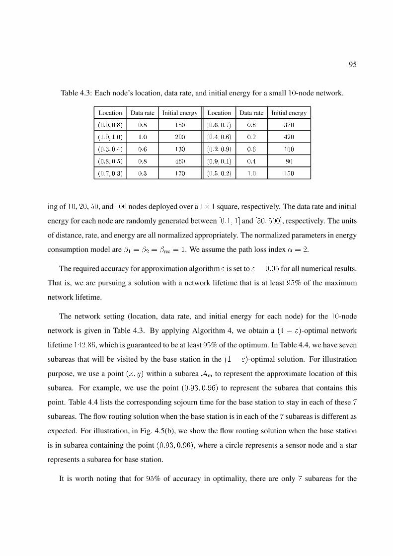
95

Table 4.3: Each node’s location, data rate, and initial energy for a small ��-node network.


��#�� #�� #� �� #�� #�� #� ��

��#�� #�� #� �� #�� #�� # ��

��#�� #�� #� �� #� �#�� #� ��

��#�� #�� #� �� #�� #�� #� ��

��#�� #�� #� �� #�� #� �#� ��

ing of ��, ��, ��, and �� nodes deployed over a �� square, respectively. The data rate and initial

energy for each node are randomly generated between �� and �� , respectively. The units

of distance, rate, and energy are all normalized appropriately. The normalized parameters in energy

consumption model are � � � � rec � �. We assume the path loss index � � �.

The required accuracy for approximation algorithm � is set to � � �� for all numerical results.

That is, we are pursuing a solution with a network lifetime that is at least ��% of the maximum

network lifetime.

The network setting (location, data rate, and initial energy for each node) for the ��-node

network is given in Table 4.3. By applying Algorithm 4, we obtain a �� -optimal network

lifetime ��, which is guaranteed to be at least ��% of the optimum. In Table 4.4, we have seven

subareas that will be visited by the base station in the �� -optimal solution. For illustration

purpose, we use a point �� )� within a subarea �� to represent the approximate location of this

subarea. For example, we use the point �� to represent the subarea that contains this

point. Table 4.4 lists the corresponding sojourn time for the base station to stay in each of these �

subareas. The flow routing solution when the base station is in each of the � subareas is different as

expected. For illustration, in Fig. 4.5(b), we show the flow routing solution when the base station

is in subarea containing the point �� , where a circle represents a sensor node and a star

represents a subarea for base station.

It is worth noting that for ��% of accuracy in optimality, there are only � subareas for the

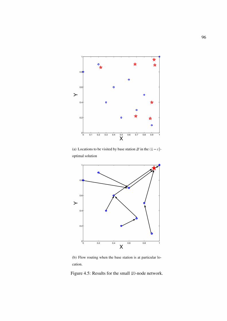
96

0 0.1 0.2 0.3 0.4 0.5 0.6 0.7 0.8 0.9 10

0.2

0.4

0.6

0.8

1

X

Y

(a) Locations to be visited by base station � in the �� -

optimal solution

0 0.2 0.4 0.6 0.8 10

0.2

0.4

0.6

0.8

1

X

Y

(b) Flow routing when the base station is at particular lo-

cation.

Figure 4.5: Results for the small ��-node network.

97

Table 4.4: �� -optimal result for the small ��-node network with � � ��.

��&� '� $ �� &� '� $ ��

��#�� #�� #� ��#�� #�� #��

��#�� #�� #�� #�� #�� #��

��#�� #� ��#�� #�� #�� #��

��#�� #�� #��

Table 4.5: Each node’s location, data rate, and initial energy for a ��-node network.


��#�� #�� #� �� #�� #�� #� ��

��#�� #�� #� �� #�� #�� #� ��

��#�� #�� #� �� #�� #�� #� ��

��#�� #�� #� � ��#�� #�� #� ��

��#�� #�� #� �� #�� #�� #� �

��#�� #�� #� �� #�� #�� #� ��

��#�� #�� #� �� #�� #�� #� ��

��#�� #�� #� �� #�� #�� # ��

��#�� #�� #� �� #�� #�� #� ��

��#�� #�� #� �� #�� #�� #� ��

base station to visit. It turns out that for ��, ��, and �� node networks, the number of subareas

that needs to be visited by the base station is still very small (� subareas for ��-node network, �

subareas for ��-node network, and �� subareas for ��-node network). This new observation is

not obvious. But it is a good news as it hints that the base station does not need to be involved in

frequent movement to achieve near-optimal solution.

The network setting for a ��-node network (with location, data rate, and initial energy for each

of the �� sensor nodes) is given in Table 4.5. By applying Algorithm 4, we obtain the �� -

optimal network lifetime ��, which is guaranteed to be at least within ��% of the optimal.

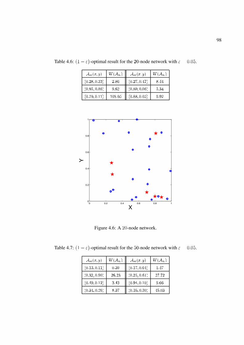
98

Table 4.6: �� -optimal result for the ��-node network with � � ��.

��&� '� $ �� &� '� $ ��

��#�� #�� #�� #�� #�� #��

��#�� #�� #� ��#�� #�� #��

��#�� #�� #�� #�� #�� #�

0 0.2 0.4 0.6 0.8 10

0.2

0.4

0.6

0.8

1

X

Y

Figure 4.6: A ��-node network.


��&� '� $ �� &� '� $ ��

��#�� #�� #�� #�� #�� #��

��#�� #�� #� ��#�� #�� #�

��#�� #�� #�� #�� #�� #��

��#�� #�� #�� #�� #�� #��

99

0 0.2 0.4 0.6 0.8 10

0.2

0.4

0.6

0.8

1

X

Y

Figure 4.7: A ��-node network used in numerical investigation.

Again, we use a point within the chosen subarea � to represent the approximate location of this

subarea. For this particular ��-node network setting, we have � subarea in the final solution, with

the corresponding sojourn time in each subarea listed in Table 4.6.

For the ��-node network, the positions of the nodes are shown in Fig. 4.7, where a circle

represents a sensor node and a star represents an optimal subarea for base station. The data rate

and initial energy for each node are randomly generated between �� and �� , respectively.

By applying Algorithm 4, we obtain a �� -optimal network lifetime ��. Again, we use a

point within a subarea�� to represent the approximate location of this subarea. For this particular

��-node network setting, we have � subareas that the base station should visit in the final solution,

with the corresponding sojourn time in each subarea listed in Table 4.7.

Finally, we consider a ��-node network shown in Fig. 4.8. The data rate and initial energy for

each node are again randomly generated between �� and �� , respectively. By applying

Algorithm 4, we have a �� -optimal network lifetime ��. For this particular ��-node

network setting, we have �� subareas that the base station should visit in the solution, with the

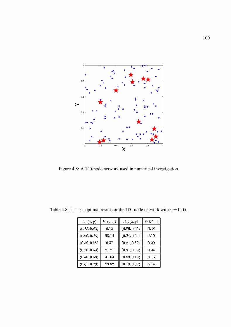
100

0 0.2 0.4 0.6 0.8 10

0.2

0.4

0.6

0.8

1

X

Y

Figure 4.8: A ��-node network used in numerical investigation.


��&� '� $ �� &� '� $ ��

��#�� #�� #�� #�� #�� #��

��#�� #�� #�� #�� #�� #��

��#�� #�� #�� #�� #�� #��

��#�� #�� #� ��#�� #�� #��

��#�� #�� #�� #�� #�� #��

��#�� #�� #� ��#�� #�� #��

101

corresponding sojourn time in each subarea listed in Table 4.8.

4.6 Related Work

Energy efficient routing has been an active area of research for sensor network in recent years

(e.g., [86,92,96,105]). It is now well understood that energy efficient routing differs from lifetime-

optimal routing as the former advocates the use of minimum energy-cost path, which may overload

nodes along some common shared path, leading to poor performance in network lifetime.

Routing algorithms to maximize network lifetime has been an active area of research even for

fixed base station location (see, e.g., [15, 17, 18, 87] and references therein). The focus is mainly

devoted to how to split traffic flow along different routes and how to adjust power level at each node

so that some optimal flow routing topology can be set up to maximize network lifetime. These

early work have laid foundation on the importance of power control and flow routing topology on

network lifetime performance.

There are some recent work on optimal base station placement [32, 73]. The focus on these

efforts is on finding an optimal fixed position for the base station so that network lifetime can be

maximized. However, as pointed out in [62,110], network lifetime can be substantially increased if

the optimization space can be expanded to include movement of the base station during the course

of sensor network operation.

Relevant work in the area of mobile base station for network lifetime problems include [5,

37, 62, 104, 110]. In [5, 37, 104], the locations of base station are constrained on a set of “pre-

determined” locations. In [110], Younis et al. show that mobile base station can increase network

lifetime. In [62], Luo and Hubaux propose to minimize the maximum load on a node among all

the nodes in the network, which can be considered as an equivalent problem to maximize network

lifetime. The results in [62, 110] are heuristic, and thus do not provide any theoretical bound on

network lifetime performance.

102

Note that the mobile base station problem considered in this chapter differs fundamentally

from the delay-tolerant network (DTN) (e.g., [53, 113]). DTN is assumed to experience frequent

and long duration partition. The focus is to leverage storage at the intermediate nodes over long

period of time and perform intermittent routing “over time” (i.e., delay tolerant) so as to achieve

“eventual delivery”. Network lifetime is not a major performance objective in the context of DTN.

4.7 Conclusions

The benefits of employing mobile base station to prolong sensor network lifetime are significant.

However, due to the complexity of the problem (time-dependent network topology and traffic

routing), provably optimal theoretical results have remained an open research area before this

chapter. This chapter fills in this important gap by contributing a provably optimal algorithm

regarding the movement of a mobile base station. The foundation of our result hinges upon a novel

time-to-space transformation for problem formulation. Based on this transformation, we present

an intermediate result which says that when the location of the base station are constrained to be on

a set of pre-determined points, then the optimal solution can be obtained via a single LP. Building

upon this intermediate result, our main result addressed the general mobile base station problem

where the location of the base station is un-constrained. We developed a provably �� -optimal

algorithm for the mobile base station problem such that the network lifetime is guaranteed to be

at least �� of the maximum network lifetime, where � � � can be made arbitrarily small

depending on required precision.

Chapter 5

Optimal Spectrum Sharing for CR

Networks

5.1 Introduction

Recent studies sponsored by the FCC have shown that traditional fixed spectrum allocation policy

is becoming inadequate in addressing today’s rapidly evolving wireless communications. Studies

show that many allocated spectrum blocks are not used in certain geographical areas and are idle

most of the time. These frequency bands are called the spectrum “white space” or “hole” (a

bandwidth is considered white space if it is wider than � MHz and remains unoccupied for at least

�� minutes). Measurements conducted by the Shared Spectrum Company [63] find that even in

the most crowded area near downtown Washington, DC, where both government and commercial

spectrum use is intensive, 62% of the spectrum remain white space. Another measurement, also

conducted by the Shared Spectrum Company [64], shows that even during the 2004 Republican

National Convention in New York City (perhaps the most heavily-congested area in the U.S. at

that time), there was still significant white space available in the public sector spectrum. These

studies have prompted the FCC to explore new innovative policies to encourage dynamic access to

the under-utilized spectrum [35]. Wireless devices are allowed to sense and explore a wide range

103

104

of the frequency spectrum and identify currently unused spectrum blocks for data communication.

This approach is also called dynamic spectrum access (DSA).

The enabling physical layer technology to realize DSA is cognitive radio (CR), which is a

frequency-agile data communication device that has a rich control and monitoring (spectrum sens-

ing) interface [45,69]. It capitalizes advances in signal processing and radio technology, as well as

recent advancements in spectrum policy [83]. A frequency-agile radio module is capable of sens-

ing the available bands [16, 38, 39, 68, 85, 102], reconfiguring RF, and switching to newly-selected

frequency bands. Thus, a CR can be programmed to tune and operate on specific frequency bands

over a wide spectrum range [83]. An even more profound advance in CR technology is that there

is no requirement that selected frequencies/channels be contiguous: the radio can send packets

over non-contiguous frequency bands. From an application perspective, CR allows a single radio

to provide a wide variety of functions, acting as a cell phone, broadcast receiver, GPS receiver,

wireless data terminal, etc.

In this chapter, we focus on the multi-hop networking problem for a CR-based wireless net-

work. For such a network, each node senses a set of spectrum bands that it can use. Due to the

unequal size of spectrum bands, it is necessary to further divide each band into sub-bands (likely

of unequal size) to schedule transmission and reception. There are many fundamental problems

that can be posed for such a wireless network in the context of rates and capacity. In this chapter,

we consider the following problem. Suppose there is a set of user sessions in the network that is

characterized by a set of source-destination pairs each having a certain rate requirement. Then,

how can we perform spectrum allocation, scheduling and interference avoidance, and multi-hop

multi-path routing such that the required network-wide radio spectrum resource is minimized?

To formulate the problem mathematically, we characterize behaviors and constraints from mul-

tiple layers for a general multi-hop CR network. Special attention is given to modeling of spectrum

sharing and unequal (non-uniform) sub-band division, scheduling and interference modeling, and

multi-path routing. We formulate an optimization problem with the objective of minimizing the

required network-wide radio spectrum resource for a set of source-destination pair rate require-

105

ments. Since such a problem formulation is a mixed-integer non-linear program (MINLP), which

is NP-hard in general [40], we aim to derive a near-optimal solution.

We present a near-optimal algorithm for the formulated MINLP problem. First, we develop

a lower bound for the objective by relaxing the integer variables and employing a linearization

technique. This lower bound will be used as a measure for the quality of any solution. Then

we present a novel sequential fixing (SF) solution procedure where the determination of integer

variables is performed iteratively through a sequence of linear programs (LPs). Upon fixing all the

integer variables, other variables in the optimization problem can be solved using an LP. Since the

solution obtained by the proposed SF algorithm represents an upper bound for the objective, we

compare it to the lower bound developed earlier. Simulations show that the results obtained by the

SF algorithm are very close to the lower bound, thus suggesting that (1) the lower bound is very

tight; and (2) the solution obtained by the SF algorithm is even closer to the optimum and thus

is near-optimal. The significance of this theoretical work is to provide a performance benchmark

which can be used to evaluate protocols and distributed algorithms for real implementation.

The remainder of this chapter is organized as follows. In Section 5.2, we characterize the be-

havior of CR networks from multiple layers and formulate them as mathematical constraints. We

also elaborate on the optimal radio resource sharing problem and formulate it as an MINLP prob-

lem. In Section 5.3, we develop a lower bound for this MINLP problem by relaxing integer vari-

ables and using linearization. In Section 5.4, we describe the proposed SF algorithm. Section 5.5

presents simulation results and demonstrates the near-optimal performance of the SF algorithm.

In Section 5.6, we review related work on CR and state-of-the-art on cross-layer optimization for

MC-MR networks. Section 5.7 concludes this chapter.

5.2 CR Network Model and Problem Formulation

We consider an ad hoc network consisting of a set � of nodes. Among these nodes, there are a

set � of uni-cast communication sessions. Denote 2�� and �� the source and destination nodes

106


Symbol Definition

(�� Number of sub-bands in band �

� The number of available bands in the network

) Transmission power spectral density at a transmitter

)� The minimum threshold of power spectral density to decode a transmission at a receiver

) The maximum threshold of power spectral density for interference to be negligible at a receiver

� � Transmission range and interference range, respectively

*�� The fraction of bandwidth for the +-th sub-band in band �

$ �� Bandwidth of band �

&�� Binary indicator to mark whether or not sub-band �� +� is used by link �� .

of session � �, and �� the rate requirement (in b/s) of session �. Table 5.1 lists all notation that

are used only in this chapter.

5.2.1 Modeling of Multi-layer Characteristics

Modeling of Spectrum Sharing and Sub-band Division. This mathematical modeling feature

and constraints are unique to CR networks and do not exist in MC-MR networks. In a multi-hop

CR network, the available spectrum bands at one node may be different from another node in the

network. Given a set of available frequency bands at a node, the size (or bandwidth) of each band

may differ drastically. For example, among the least-utilized spectrum bands found in [64], the

bandwidth between �� MHz (allocated to amateur radio) is �� MHz, while bandwidth

between �� MHz (allocated to mobile satellites, GPS systems, and meteorological appli-

cations) is �� MHz. Such large difference in bandwidths among the available bands suggests the

need for further division of the larger bands into smaller sub-bands for more flexible and efficient

frequency allocation. Since equal sub-band division of the available spectrum band is likely to

yield sub-optimal performance, an unequal division is desirable.

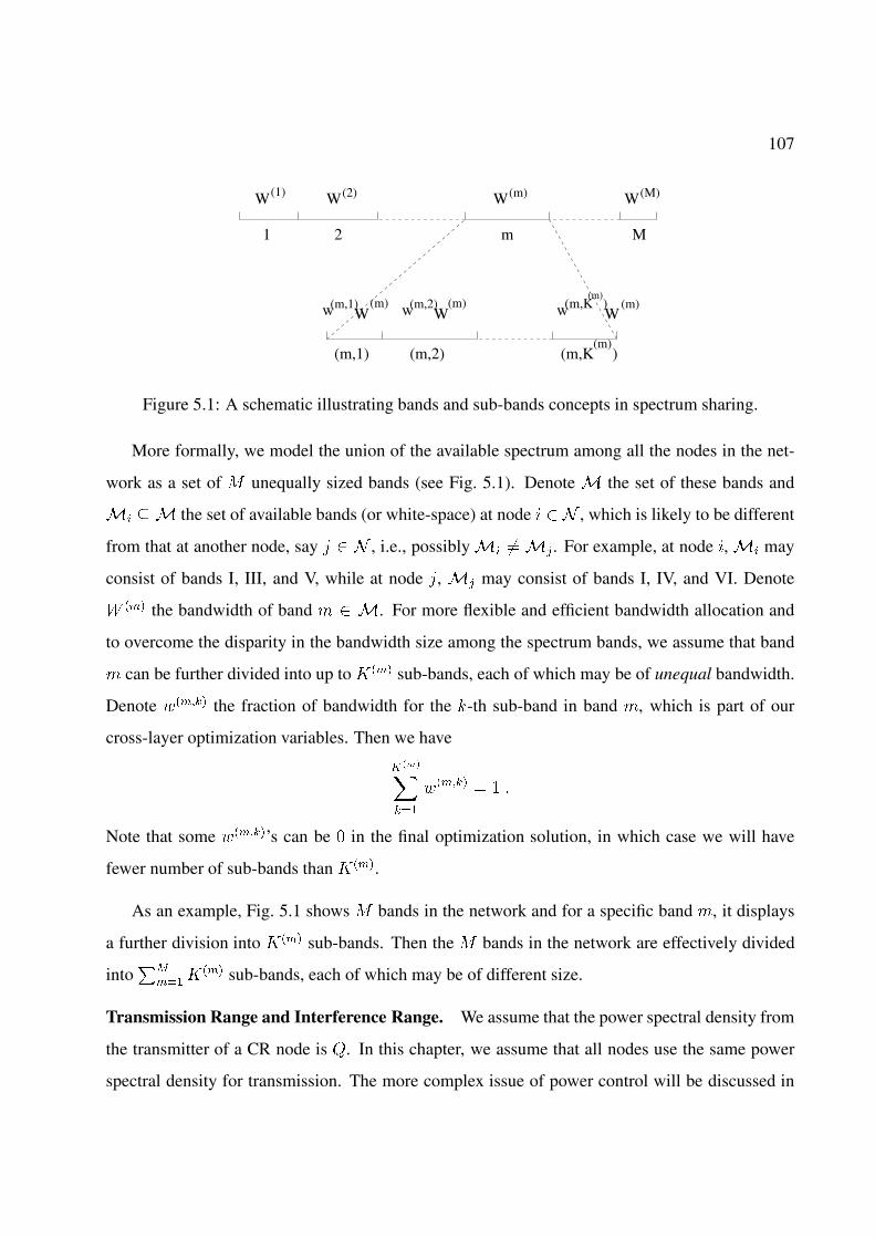
107

(1) WW(2) (m) (M)

(m)(m,K )

(m)(m,K )w(m,1)w W

(m)W

(m)(m,2)w (m)W

21 m M

(m,1) (m,2)

W W

Figure 5.1: A schematic illustrating bands and sub-bands concepts in spectrum sharing.

More formally, we model the union of the available spectrum among all the nodes in the net-

work as a set of * unequally sized bands (see Fig. 5.1). Denote � the set of these bands and

�� the set of available bands (or white-space) at node � , which is likely to be different

from that at another node, say ' � , i.e., possibly �� . For example, at node , �� may

consist of bands I, III, and V, while at node ', � may consist of bands I, IV, and VI. Denote

0 �� the bandwidth of band ! �. For more flexible and efficient bandwidth allocation and

to overcome the disparity in the bandwidth size among the spectrum bands, we assume that band

! can be further divided into up to .�� sub-bands, each of which may be of unequal bandwidth.

Denote 3�� the fraction of bandwidth for the �-th sub-band in band !, which is part of our

cross-layer optimization variables. Then we have

��

3��

Note that some 3��’s can be � in the final optimization solution, in which case we will have

fewer number of sub-bands than .��.

As an example, Fig. 5.1 shows * bands in the network and for a specific band !, it displays

a further division into .�� sub-bands. Then the * bands in the network are effectively divided

into��

�� .�� sub-bands, each of which may be of different size.

Transmission Range and Interference Range. We assume that the power spectral density from

the transmitter of a CR node is 4. In this chapter, we assume that all nodes use the same power

spectral density for transmission. The more complex issue of power control will be discussed in

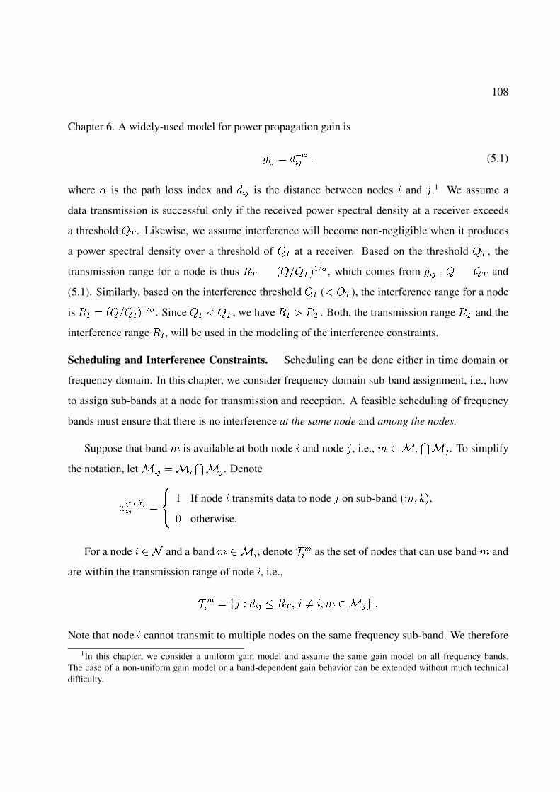
108

Chapter 6. A widely-used model for power propagation gain is

$� � �� (5.1)

where � is the path loss index and �� is the distance between nodes and '.1 We assume a

data transmission is successful only if the received power spectral density at a receiver exceeds

a threshold 4� . Likewise, we assume interference will become non-negligible when it produces

a power spectral density over a threshold of 4� at a receiver. Based on the threshold 4� , the

transmission range for a node is thus �� 4,4� ��, which comes from $� � 4 � 4� and

(5.1). Similarly, based on the interference threshold 4� (� 4� ), the interference range for a node

is �� 4,4��. Since 4� � 4� , we have �� . Both, the transmission range �� and the

interference range �� , will be used in the modeling of the interference constraints.

Scheduling and Interference Constraints. Scheduling can be done either in time domain or

frequency domain. In this chapter, we consider frequency domain sub-band assignment, i.e., how

to assign sub-bands at a node for transmission and reception. A feasible scheduling of frequency

bands must ensure that there is no interference at the same node and among the nodes.

Suppose that band ! is available at both node and node ', i.e., ! ��

� . To simplify

the notation, let ��

�. Denote

��

!"# � If node transmits data to node ' on sub-band �!� ��,

� otherwise.

For a node � and a band ! ��, denote � �� as the set of nodes that can use band ! and

are within the transmission range of node , i.e.,

� �� ' � �� ' �� ! ��

Note that node cannot transmit to multiple nodes on the same frequency sub-band. We therefore

1In this chapter, we consider a uniform gain model and assume the same gain model on all frequency bands.The case of a non-uniform gain model or a band-dependent gain behavior can be extended without much technicaldifficulty.

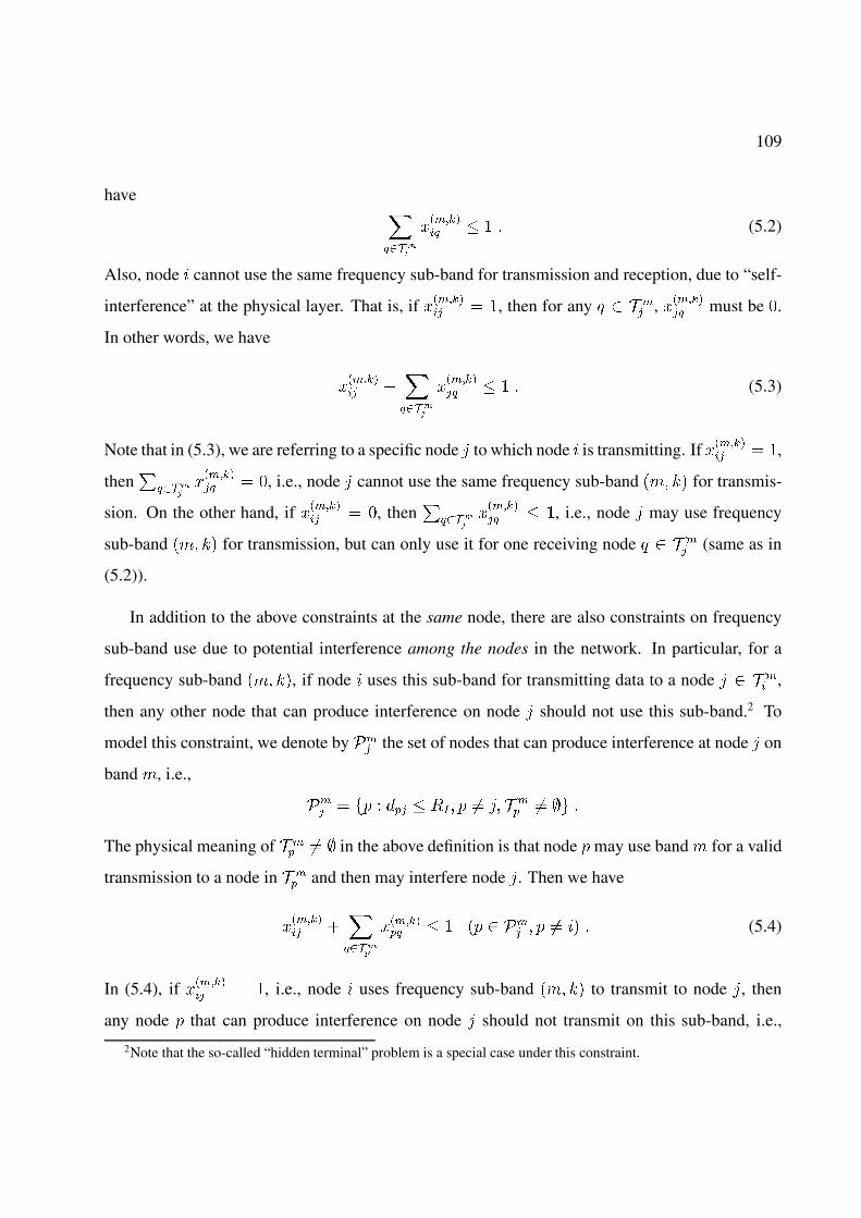
109

have ��

�

�� (5.2)

Also, node cannot use the same frequency sub-band for transmission and reception, due to “self-

interference” at the physical layer. That is, if �� , then for any � �

, �� must be �.

In other words, we have

��

��

�

�� (5.3)

Note that in (5.3), we are referring to a specific node ' to which node is transmitting. If �� ,

then�

��

�� , i.e., node ' cannot use the same frequency sub-band �!� �� for transmis-

sion. On the other hand, if �� , then

��

�� , i.e., node ' may use frequency

sub-band �!� �� for transmission, but can only use it for one receiving node � � (same as in

(5.2)).

In addition to the above constraints at the same node, there are also constraints on frequency

sub-band use due to potential interference among the nodes in the network. In particular, for a

frequency sub-band �!� ��, if node uses this sub-band for transmitting data to a node ' � �� ,

then any other node that can produce interference on node ' should not use this sub-band.2 To

model this constraint, we denote by �� the set of nodes that can produce interference at node ' on

band !, i.e.,

�� '� � �

� ��

The physical meaning of � �� in the above definition is that node may use band ! for a valid

transmission to a node in � �� and then may interfere node '. Then we have

��

��

�

��

� �� (5.4)

In (5.4), if �� , i.e., node uses frequency sub-band �!� �� to transmit to node ', then

any node that can produce interference on node ' should not transmit on this sub-band, i.e.,

2Note that the so-called “hidden terminal” problem is a special case under this constraint.

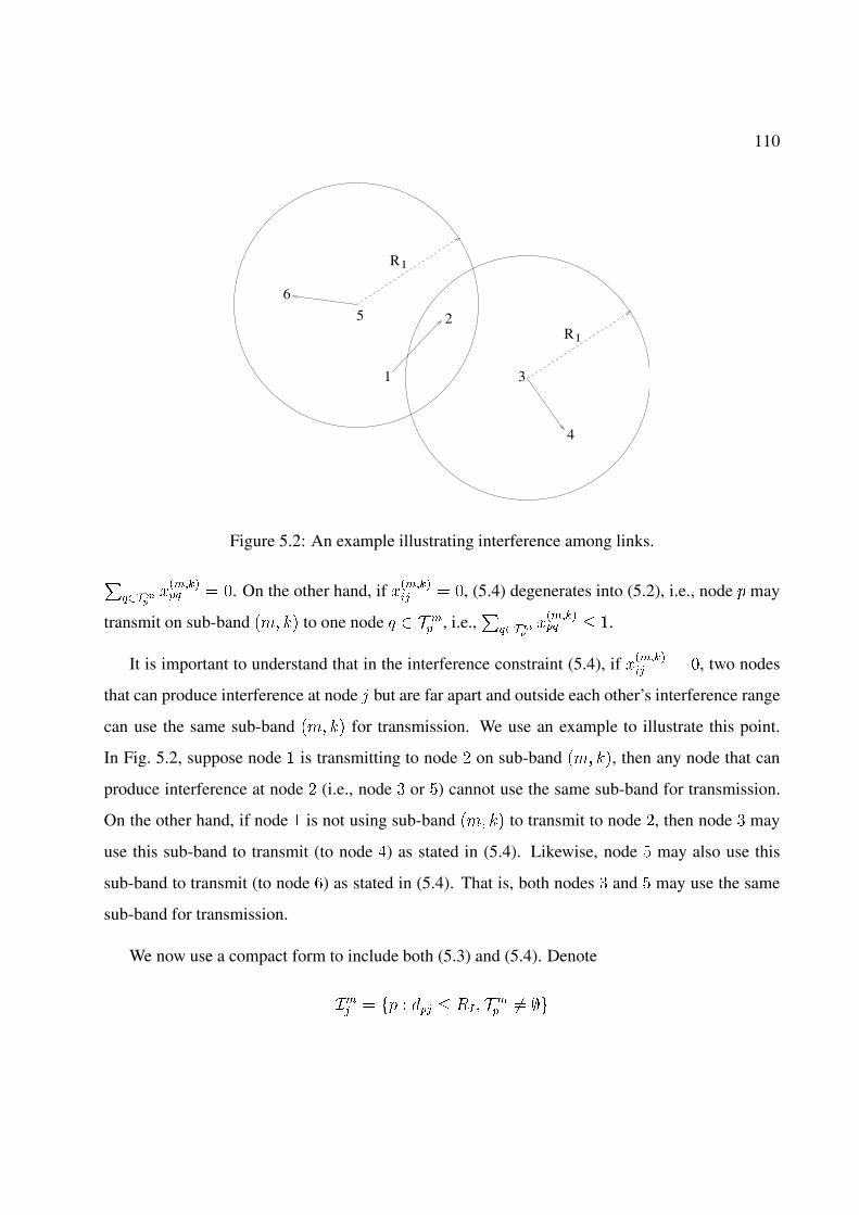
110

3

I

R I

1

2

6

5

4

R

Figure 5.2: An example illustrating interference among links.

��

�� . On the other hand, if ��

� � �, (5.4) degenerates into (5.2), i.e., node may

transmit on sub-band �!� �� to one node � �� , i.e.,

��

�� .

It is important to understand that in the interference constraint (5.4), if �� , two nodes

that can produce interference at node ' but are far apart and outside each other’s interference range

can use the same sub-band �!� �� for transmission. We use an example to illustrate this point.

In Fig. 5.2, suppose node � is transmitting to node � on sub-band �!� ��, then any node that can

produce interference at node � (i.e., node or �) cannot use the same sub-band for transmission.

On the other hand, if node � is not using sub-band �!� �� to transmit to node �, then node may

use this sub-band to transmit (to node �) as stated in (5.4). Likewise, node � may also use this

sub-band to transmit (to node �) as stated in (5.4). That is, both nodes and � may use the same

sub-band for transmission.

We now use a compact form to include both (5.3) and (5.4). Denote

��

111

which is equivalent to

��

!"# ��

��'� If � �

��

�� otherwise �

Thus, both (5.3) and (5.4) can be described by the following constraint.

��

��

�

��

Routing. At the network level, a source node may need a number of relay nodes to route the data

stream toward its destination node. Clearly, a route having a single path may be overly restrictive

and is not able to take advantage of load balancing. A set of paths (or multi-path) is more flexible

to route the traffic from a source node to its destination. Mathematically, this can be modeled as

follows.

Denote �� the data rate on link � ' that is attributed to session �, where � � ' ��

� �� , and � �. To simplify the notation, let ��

��

� �� . If node is the source node

of session �, i.e., � 2��, then

��

�� (5.5)

If node is an intermediate relay node for session �, i.e., �� 2�� and �� , then

��

��

��

�� (5.6)

If node is the destination node of session �, i.e., � ��, then

��

�� (5.7)

It can be easily verified that if (5.5) and (5.6) are satisfied, then (5.7) must be satisfied. As a result,

it is sufficient to list only (5.5) and (5.6) in the formulation.

In addition to the above flow balance equations at each node for each session �, the aggregate

flow rates on each radio link cannot exceed this link’s capacity. To model this mathematically, we

112

need to first find the capacity on link � � '� in sub-band �!� ��. If node sends data to node ' on

sub-band �!� ��, i.e., �� , then the capacity on link � ' in sub-band �!� �� is

�� 3��0 ��

��

$�4

5

��

where 5 is the ambient Gaussian noise density. Note that the denominator inside the log function

contains only 5. This is due to one of our interference constraints stated earlier, i.e., when node

is transmitting to node ' on sub-band �!� ��, then all the other neighbors of node ' within its in-

terference range are prohibited from using this sub-band. This interference constraint significantly

helps to simplify the calculation of the link capacity �� . When �

�� , we have �

�� .

Thus, �� can be written in the following compact form.

��

�� 3��0 ��

��

$�4

5

�� (5.8)

Now, returning to our earlier requirement that the aggregate data rates on each link � '

cannot exceed the link’s capacity, we have,

��

��

��

��

��

��

��

�� 3��0 ��

��

$�4

5

��

5.2.2 Problem Formulation

For the multi-hop CR networks that we are investigating, various performance objectives can be

used. In this chapter, we use the total required radio resource to support the user sessions as our

performance objective. The radio resource can be measured in terms of the total bandwidth used

by all nodes in the network, which is the simplified form of the so-called space-bandwidth product

proposed in [61] when the transmission power spectral density is fixed. It is not hard to see that

the solution procedure in this chapter can be applied when other performance objectives are used.

To re-cap, we are given a set of source-destination pairs (user sessions) in the network, each

with a certain rate requirement. Each node in the network has a set of available frequency bands

that it can use for communication. We want to find an optimal solution to divide the set of avail-

able frequency bands at each node, the scheduling of sub-bands for transmission and reception,

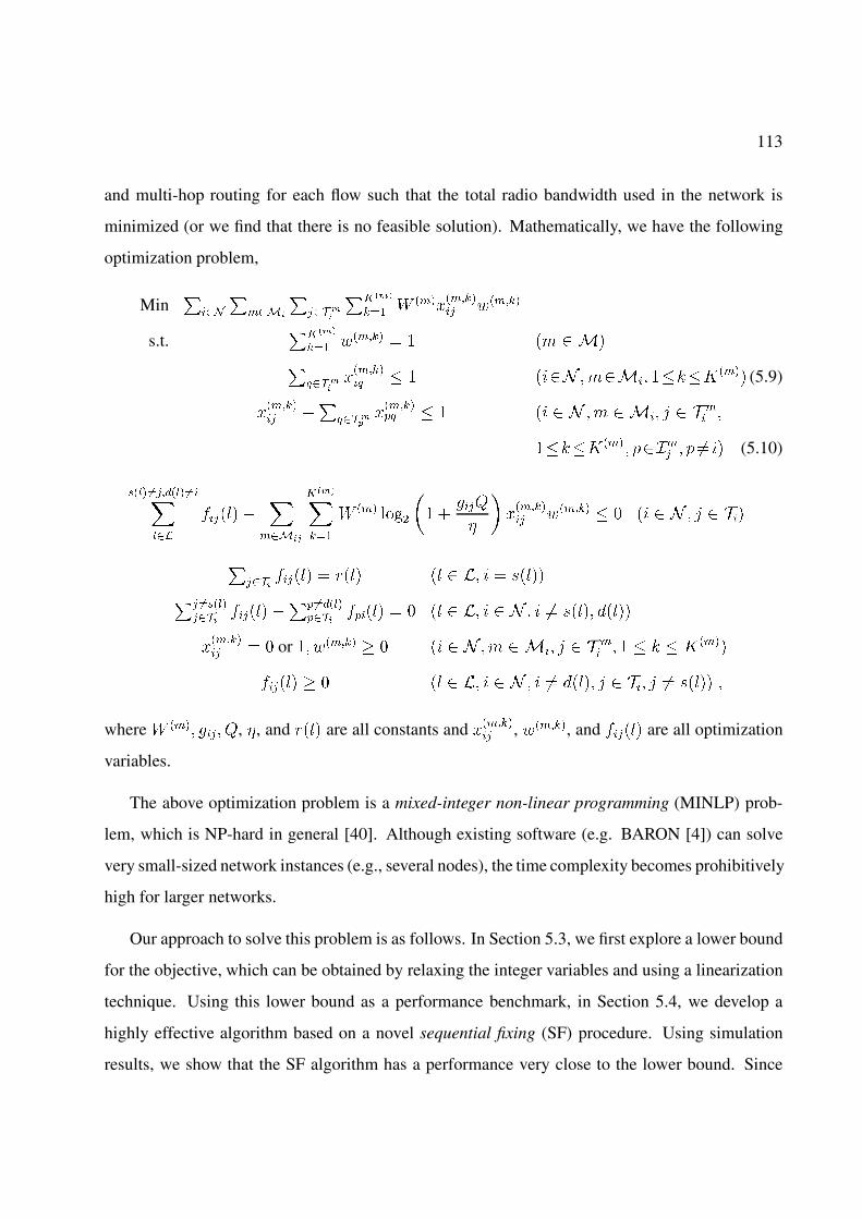
113

and multi-hop routing for each flow such that the total radio bandwidth used in the network is

minimized (or we find that there is no feasible solution). Mathematically, we have the following

optimization problem,

Min�

��

��

��

�

��

�� 0 �� 3��

s.t.��

�� 3�� ! ��

�� !�� .�� (5.9)

��

��

�� ! �� ' �

��

��.�� (5.10)

��

��

��

��

0 ��

��

$�4

5

�� 3�� ' ��

��

�� 2��

��

�� 2��

�� or �� 3�� ! �� ' �

�� .��

�� ' �� ' �� 2��

where 0 �� $�� 4, 5, and �� are all constants and �� , 3��, and �� are all optimization

variables.

The above optimization problem is a mixed-integer non-linear programming (MINLP) prob-

lem, which is NP-hard in general [40]. Although existing software (e.g. BARON [4]) can solve

very small-sized network instances (e.g., several nodes), the time complexity becomes prohibitively

high for larger networks.

Our approach to solve this problem is as follows. In Section 5.3, we first explore a lower bound

for the objective, which can be obtained by relaxing the integer variables and using a linearization

technique. Using this lower bound as a performance benchmark, in Section 5.4, we develop a

highly effective algorithm based on a novel sequential fixing (SF) procedure. Using simulation

results, we show that the SF algorithm has a performance very close to the lower bound. Since

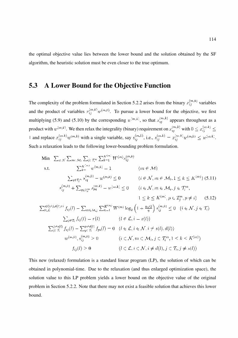
114

the optimal objective value lies between the lower bound and the solution obtained by the SF

algorithm, the heuristic solution must be even closer to the true optimum.

5.3 A Lower Bound for the Objective Function

The complexity of the problem formulated in Section 5.2.2 arises from the binary �� variables

and the product of variables �� 3��. To pursue a lower bound for the objective, we first

multiplying (5.9) and (5.10) by the corresponding 3��, so that �� appears throughout as a

product with 3��. We then relax the integrality (binary) requirement on �� with � � �

��

� and replace �� 3�� with a single variable, say 2��

� , i.e., 2��

� 3�� 3��.

Such a relaxation leads to the following lower-bounding problem formulation.

Min�

��

��

��

��

�� 0 ��2��

s.t.��

�� 3�� ! ��

�2�� 3�� ! �� .�� (5.11)

2��

��

�2�� 3�� ! �� ' �

��

� � � � .�� (5.12)��

��

��

�� 0 ��

��

��!

"

�2�� ' ��

�� 2��

��

��

�� 2��

3�� 2�� ! �� ' �

�� .��

�� ' �� ' �� 2��

This new (relaxed) formulation is a standard linear program (LP), the solution of which can be

obtained in polynomial-time. Due to the relaxation (and thus enlarged optimization space), the

solution value to this LP problem yields a lower bound on the objective value of the original

problem in Section 5.2.2. Note that there may not exist a feasible solution that achieves this lower

bound.

115

Nevertheless, this lower bound offers a benchmark to measure the quality of a feasible solution,

which we will develop in the next section. It turns out that this lower bound is extremely tight (see

results in Section 5.4). This can be explained by the convex hull results presented by Sherali et

al. [88].

5.4 A Near-Optimal Algorithm Based on Sequential Fixing

5.4.1 Basic Algorithm

We now take a closer look at the original MINLP problem formulation in Section 5.2.2. Observe

that once the binary values for all � variables are determined, i.e., whether or not a node will

indeed use a particular sub-band to send data to another node, then this MINLP reduces to an LP,

which can be solved in polynomial-time. In other words, the key obstacle in solving this MINLP

problem lies in the determination of the binary values for the � variables. To this end, we propose a

two-step solution procedure: i) fix the binary values for � variables iteratively through a sequence

of LPs; ii) once all the � variables are fixed, find a solution (to determine how to divide sub-bands

and flow routing) corresponding to this set of � values. Such a two-step approach will yield a sub-

optimal (upper bound) solution to the original MINLP problem. The quality of this algorithm can

be assessed by how close its solution is to the lower bound we developed in the previous section.

As said, the key to the two-step approach resides in the determination of the binary values

for all the � variables. Our main idea is to fix (set) the values of the � variables sequentially

through solving a series of relaxed LP problems, with each iteration setting at least one binary

value for some �� . Specifically, during the first iteration, we relax all binary variables �

�� to

� � �� as in Section 5.3 to obtain an LP. Upon solving this LP, we have a solution with

each �� 2

�� ,3�� being a value between � and �. Among all the � values, suppose some

�� has the largest value. Then we fix (set) this particular ��

� to 1. As a result of this fixing,

by (5.9), we also need to fix �� for � �

� and �� '. By (5.10), we also fix �� to �

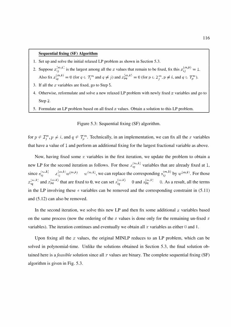
116

Sequential fixing (SF) Algorithm

1. Set up and solve the initial relaxed LP problem as shown in Section 5.3.

2. Suppose �� is the largest among all the � values that remain to be fixed, fix this ��

� � �.

Also fix �� (for � � � �

� and � �� ) and �� (for � �� , and � � � �

� ).

3. If all the � variables are fixed, go to Step �.

4. Otherwise, reformulate and solve a new relaxed LP problem with newly fixed � variables and go to

Step �.

5. Formulate an LP problem based on all fixed � values. Obtain a solution to this LP problem.

Figure 5.3: Sequential fixing (SF) algorithm.

for �� , and � �� . Technically, in an implementation, we can fix all the � variables

that have a value of � and perform an additional fixing for the largest fractional variable as above.

Now, having fixed some � variables in the first iteration, we update the problem to obtain a

new LP for the second iteration as follows. For those �� variables that are already fixed at �,

since 2��

� 3�� 3��, we can replace the corresponding 2�� by 3��. For those

�� and �

�� that are fixed to �, we can set 2��

�� and 2�� . As a result, all the terms

in the LP involving these 2 variables can be removed and the corresponding constraint in (5.11)

and (5.12) can also be removed.

In the second iteration, we solve this new LP and then fix some additional � variables based

on the same process (now the ordering of the � values is done only for the remaining un-fixed �

variables). The iteration continues and eventually we obtain all � variables as either � and �.

Upon fixing all the � values, the original MINLP reduces to an LP problem, which can be

solved in polynomial-time. Unlike the solutions obtained in Section 5.3, the final solution ob-

tained here is a feasible solution since all � values are binary. The complete sequential fixing (SF)

algorithm is given in Fig. 5.3.

117

5.4.2 An Iteration-Speedup Technique

In the SF algorithm, we need to solve a sequence of LPs. The complexity of SF is polynomial.

By exploiting the space and frequency dimensions involved in radio resource allocation, we may

decrease the number of LPs by fixing more � variables during each iteration in Fig. 5.3. As a

result, the complexity can be further decreased. From a space dimension viewpoint, a sub-band

usage will only have an impact within the interference range and the same sub-band can be used by

other links outside this range. Thus, for the same sub-band �!� ��, we can then fix multiple links

that have non-overlapping interference ranges within a single iteration of the sequential fixing

algorithm. From the frequency dimension viewpoint, the transmission in one sub-band will not

interfere with the transmission in a different sub-band. Thus, for the same link � ', we can

then fix multiple sub-bands within a single iteration of the SF algorithm. Specifically, we can use

a threshold � � �� in this fixing process and fix all the � variables that exceeds � to � in a single

iteration. Note that in (5.9) and (5.10), it is required that at most one binary variable ��

while in the relaxed problem, there is at most one fraction 2�� ,6�� . Thus, � � ��

ensures that both the constraints (5.9) and (5.10) (interference constraints at each node and among

the nodes) will hold during the SF procedure.3 In the case that none of the � variables exceed �,

we will fall back to the basic algorithm in Fig. 5.3 and simply choose the largest valued � variable.

5.5 Simulation Results

In this section, we present simulation results for our SF algorithm and compare them to the lower

bounds obtained in Section 5.3. The units for distance, rate, and power density satisfy (5.1) and

(5.8) and are all normalized with appropriate dimensions. We consider � � �� or �� nodes

in a ��x�� area. Among these nodes, there are � � � active sessions, each with a rate within

�� .

We assume that there are * � � bands that can be used for the entire network (see Table 5.2).

3We use � � �#�� in our simulation results.

118

Table 5.2: Available bands among all nodes in the network in the simulation study.

Band Index Spectrum Range (MHz) Bandwidth (MHz)

I �� #�

II �� #�

III �� #�

IV �� #�� #�

V �� #�

Bands I and II are among the least-utilized (less than 2%) spectrum bands found in [64] and bands

III, IV, and V are unlicensed ISM bands used for 802.11. Recall that available bands at each CR

node is a subset of these five bands based on its location and the available bands at any two nodes

in the network may not be identical. In the simulation, this is done by randomly selecting a subset

of bands from the pool of five bands for each node. Further, we assume bands I to V can be divided

into up to � �� , and � sub-bands although other desirable divisions can be used. Note that the

size of each sub-band may be unequal and is part of the optimization problem.

We assume that the transmission range at each node is �� and that the interference range is �,

although other settings can be used. The path loss index � is assumed to be �. The threshold 4�

is assumed to be 5. Thus, we have 4� �$��

%�4� � ��

��5 and the transmission power spectral

density 4 � ��4� � �� 5.

Note that it is possible that there is no feasible solution for a specific data set. This could be

attributed to dis-connectivity in the network (due to random network topology), resource bottleneck

in a hot area, etc. Thus, we only report results based on those data sets that have feasible solutions.

We first present simulation results for �� data sets for ��-node networks that can produce

feasible solutions. For each data set, the network topology, source/destination pair and bit rate of

each session, and available frequency bands at each node are randomly generated. We use the SF

Algorithm to determine the cost, which is the total required bandwidth in the objective function.

As discussed, we compare this result with the lower bound developed in Section 5.3. The running

119

1 10 20 30 40 50 60 70 80 90 1000

0.2

0.4

0.6

0.8

1

1.2

1.4

1.6

1.8

2

Set Index

Nor

mal

ized

Cos

t(w

.r.t.

Low

er B

ound

)

Figure 5.4: Normalized cost (with respect to lower bound) for �� data sets of ��-node networks.

time for each simulation is less than �� seconds on a Pentium �� GHz machine.

Figure 5.4 shows the normalized costs obtained by the SF algorithm with respect to the lower

bound costs for �� data sets. The average normalized cost among the �� simulations is �� and

the standard derivation is ��. There are two observations that can be made from this figure. First,

since the ratio of the solution obtained by SF (upper bound of optimal solution) to the lower bound

solution is close to � (in many cases, they coincide with each other), the gap between them is very

small. Second, since the optimal solution (unknown) is between the solution obtained by the SF

algorithm and the lower bound, the lower bound is very tight; more importantly, the SF solution

must be even closer to the optimum.

To get a sense of how the actual (rather than normalized) numerical results appear in the simula-

tions, we list the first �� sets of results in Table 5.3. Note that in many cases, the result obtained by

the SF algorithm is identical to the respective lower bound obtained via relaxation. This indicates

that the solution found by SF is optimal.

Simulation results for �� random data sets for �-node and ��-node networks that produce

feasible solutions are displaced in Figs. 5.5(a) and (b), respectively. For �-node networks, the

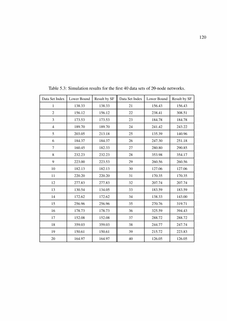
120

Table 5.3: Simulation results for the first 40 data sets of ��-node networks.

Data Set Index Lower Bound Result by SF Data Set Index Lower Bound Result by SF

1 138.33 138.33 21 156.43 156.43

2 156.12 156.12 22 238.41 308.51

3 173.53 173.53 23 184.78 184.78

4 189.70 189.70 24 241.42 243.22

5 203.05 213.18 25 135.39 140.96

6 184.37 184.37 26 247.30 251.18

7 160.45 182.33 27 280.80 290.85

8 232.23 232.23 28 353.98 354.17

9 223.00 223.53 29 260.56 260.56

10 182.13 182.13 30 127.06 127.06

11 220.20 220.20 31 170.35 170.35

12 277.83 277.83 32 207.74 207.74

13 130.54 134.05 33 183.59 183.59

14 172.62 172.62 34 138.33 143.00

15 256.96 256.96 35 270.76 319.71

16 178.73 178.73 36 325.59 394.43

17 152.08 152.08 37 288.72 288.72

18 359.03 359.03 38 244.77 247.74

19 150.61 150.61 39 215.72 223.83

20 164.97 164.97 40 126.05 126.05

121

1 10 20 30 40 50 60 70 80 90 1000

0.2

0.4

0.6

0.8

1

1.2

1.4

1.6

1.8

2

Set Index

Nor

mal

ized

Cos

t(w

.r.t.

Low

er B

ound

)

(a) �� data sets of ��-node networks.

1 10 20 30 40 50 60 70 80 90 1000

0.2

0.4

0.6

0.8

1

1.2

1.4

1.6

1.8

2

Set Index

Nor

mal

ized

Cos

t(w

.r.t.

Low

er B

ound

)

(b) �� data sets of ��-node networks.

Figure 5.5: Normalized cost (with respect to lower bound).

122

average normalized cost among the �� simulations is �� and the standard derivation is ��. For

��-node networks, the average normalized cost among the �� simulations is �� and the standard

derivation is ��. Thus, the SF solutions are also close to the optimal solutions.

5.6 Related Work

CR is based on software defined radio (SDR) [83]. Since its inception, SDR development has

witnessed rapid advances. Standards bodies such as IEEE 802 Standards Committee, the SDR Fo-

rum, the Object Management Group have been instrumental in promoting open standards for SDR

commercialization. Among others, the Software Communications Architecture core framework is

the result from standardization efforts on SDR. The IEEE 802.22 working group is in the process

of developing a standard for a CR interface for license-exempt devices on a non-interfering basis

in spectrum that is allocated to the TV Broadcast Service. CR employs all the SDR technologies,

plus the additional capability of spectrum sensing and cognition (learning and adaptation).

In CR research community, there have been extensive activities devoted to effective sharing

of spectrum or spectrum allocation. For a multi-user single-hop communication in a network

environment, a number of approaches have been proposed. For example, in [22, 72], game theory

was applied to study spectrum sharing, while in [50, 51], pricing mechanism was used. In [34],

Etkin et al. studied a utility maximization problem and solved it under certain condition. In [74],

Peng et al. studied the spectrum assignment problem with the aim of maximizing the total utility.

In these efforts, routing is not part of the problem.

For the multi-hop networking problem with CRs, there is limited amount of work to date avail-

able in the literature. In [112], Zhao et al. designed a distributed coordination approach for

spectrum sharing. They showed that this approach offers throughput improvement over a dedi-

cated channel approach. In [101], Ugarte and McDonald studied the network capacity problem for

multi-hop CR networks and found an upper bound, although it is not clear how tight this bound is.

In [108], Xin et al. studied how to assign frequency bands at each node to form a topology such

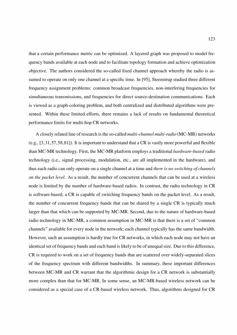
123

that a certain performance metric can be optimized. A layered graph was proposed to model fre-

quency bands available at each node and to facilitate topology formation and achieve optimization

objective. The authors considered the so-called fixed channel approach whereby the radio is as-

sumed to operate on only one channel at a specific time. In [95], Steenstrup studied three different

frequency assignment problems: common broadcast frequencies, non-interfering frequencies for

simultaneous transmissions, and frequencies for direct source-destination communications. Each

is viewed as a graph-coloring problem, and both centralized and distributed algorithms were pre-

sented. Within these limited efforts, there remains a lack of results on fundamental theoretical

performance limits for multi-hop CR networks.

A closely related line of research is the so-called multi-channel multi-radio (MC-MR) networks

(e.g., [3,31,57,58,81]). It is important to understand that a CR is vastly more powerful and flexible

than MC-MR technology. First, the MC-MR platform employs a traditional hardware-based radio

technology (i.e., signal processing, modulation, etc., are all implemented in the hardware), and

thus each radio can only operate on a single channel at a time and there is no switching of channels

on the packet level. As a result, the number of concurrent channels that can be used at a wireless

node is limited by the number of hardware-based radios. In contrast, the radio technology in CR

is software-based; a CR is capable of switching frequency bands on the packet level. As a result,

the number of concurrent frequency bands that can be shared by a single CR is typically much

larger than that which can be supported by MC-MR. Second, due to the nature of hardware-based

radio technology in MC-MR, a common assumption in MC-MR is that there is a set of “common

channels” available for every node in the network; each channel typically has the same bandwidth.

However, such an assumption is hardly true for CR networks, in which each node may not have an

identical set of frequency bands and each band is likely to be of unequal size. Due to this difference,

CR is required to work on a set of frequency bands that are scattered over widely-separated slices

of the frequency spectrum with different bandwidths. In summary, these important differences

between MC-MR and CR warrant that the algorithmic design for a CR network is substantially

more complex than that for MC-MR. In some sense, an MC-MR-based wireless network can be

considered as a special case of a CR-based wireless network. Thus, algorithms designed for CR

124

networks can be tailored to address MC-MR networks, while the converse is not true.

5.7 Conclusions

In this chapter, we conducted a systematic study on the important problem of multi-hop networking

with CR nodes. The nature of the problem calls for a characterization and modeling of multi-

layer behaviors and constraints. We characterized behaviors and constraints for a multi-hop CR

network from multiple layers, including the modeling of spectrum sharing and sub-band division,

scheduling and interference constraints, and flow routing. We formulated an optimization problem

with the objective of minimizing the required network-wide radio spectrum resource for a set

of user sessions. Since the problem formulation is an MINLP, we developed a lower bound to

estimate the objective function. Subsequently, we developed a novel sequential fixing algorithm

to the cross-layer optimization problem. Simulation results showed that results obtained by this

algorithm are very close to the lower bound, thus confirming that they are near-optimal.

Chapter 6

Optimal Power Control for CR Networks

6.1 Introduction

Cognitive radio (CR) is a revolution in radio technology and is enabled by recent advances in RF

design, signal processing, and communication software [83]. Fundamental characteristics of CR

are that transmitted waveforms are defined by software and that received waveforms are demod-

ulated by software. This is in contrast to traditional hardware-based radios in which processing

is done entirely by custom-made hardware circuitry. CR promises unprecedented flexibility in ra-

dio communications and is viewed as an enabling technology for dynamic spectrum access. Its

capability has been recognized by the military and commercial sector and is now under intensive

research and development by the DoD’s Joint Tactical Radio System (JTRS) program [54] and

wireless industry.

Since transmitted waveform is defined by software, a CR is capable of reconfiguring RF (on

the fly) and switching to newly-selected frequency bands. From networking perspective, the emer-

gence of CR offers new challenges in algorithm and protocol design. It is important to realize that

a CR is vastly more powerful and flexible than the so-called multi-channel multi-radio (MC-MR)

technology that has been actively researched in recent years (see e.g., [3, 31, 57, 58, 81] and refer-

125

126

ence therein). Note that MC-MR remains hardware-based radio technology: each radio can only

operate on a single channel at a time and the number of concurrent channels that can be used at

a wireless node is limited by the number of radio interfaces. In addition, an MC-MR based wire-

less network typically assumes there is a set of “common channels” available for all nodes in the

network. This assumption is hardly true for CR networks since each node may have a different set

of frequency bands based on its particular location. These important differences between MC-MR

and CR warrant that the algorithm design for a CR network is substantially more complex than

that under MC-MR. From algorithm design perspective, an MC-MR based wireless network can

be viewed as a special case of a CR-based wireless network. Thus, algorithms designed for CR

networks can be easily tailored to address MC-MR networks while the converse is not true.

In this chapter, we consider how to jointly perform power control, scheduling, and flow rout-

ing for a CR-based multi-hop wireless network. Specifically, we consider how to support a set

of user communication sessions (each with a rate requirement) by jointly optimizing power con-

trol, scheduling, and flow routing such that the required radio resource and interference area in the

network is minimized. We extend the current “protocol model” for interference modeling (more

discussion in Section 6.2). Since power control directly affects a node’s transmission range and

interference range, we find that it has profound impact on scheduling feasibility, bandwidth effi-

ciency, and problem complexity. We develop a formal mathematical model for scheduling feasibil-

ity under the influence of power control. Based on this model, the joint power control, scheduling,

and flow routing problem is subsequently formulated as a mixed integer nonlinear programming

(MINLP) problem. We develop a solution procedure based on the so-called branch-and-bound

technique. Using numerical results, we validate this solution procedure and offer additional in-

sights on the impact of power control and variable transmission/interference range on CR-based

wireless networks.

The main contributions of this chapter are the following:

� By extending the existing protocol interference model, we have developed a formal math-

ematical model for scheduling feasibility under the influence of power control (constraints

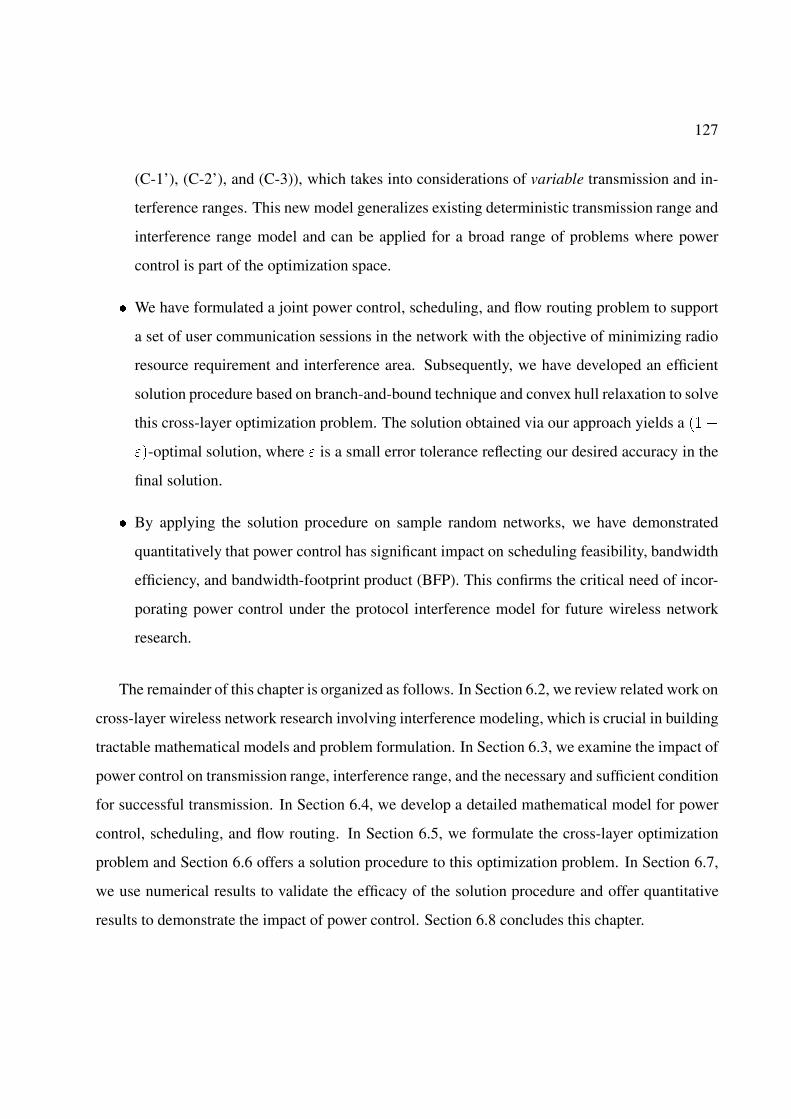
127

(C-1’), (C-2’), and (C-3)), which takes into considerations of variable transmission and in-

terference ranges. This new model generalizes existing deterministic transmission range and

interference range model and can be applied for a broad range of problems where power

control is part of the optimization space.

� We have formulated a joint power control, scheduling, and flow routing problem to support

a set of user communication sessions in the network with the objective of minimizing radio

resource requirement and interference area. Subsequently, we have developed an efficient

solution procedure based on branch-and-bound technique and convex hull relaxation to solve

this cross-layer optimization problem. The solution obtained via our approach yields a ��

��-optimal solution, where � is a small error tolerance reflecting our desired accuracy in the

final solution.

� By applying the solution procedure on sample random networks, we have demonstrated

quantitatively that power control has significant impact on scheduling feasibility, bandwidth

efficiency, and bandwidth-footprint product (BFP). This confirms the critical need of incor-

porating power control under the protocol interference model for future wireless network

research.

The remainder of this chapter is organized as follows. In Section 6.2, we review related work on

cross-layer wireless network research involving interference modeling, which is crucial in building

tractable mathematical models and problem formulation. In Section 6.3, we examine the impact of

power control on transmission range, interference range, and the necessary and sufficient condition

for successful transmission. In Section 6.4, we develop a detailed mathematical model for power

control, scheduling, and flow routing. In Section 6.5, we formulate the cross-layer optimization

problem and Section 6.6 offers a solution procedure to this optimization problem. In Section 6.7,

we use numerical results to validate the efficacy of the solution procedure and offer quantitative

results to demonstrate the impact of power control. Section 6.8 concludes this chapter.

128

6.2 Related Work

Related work on MC-MR and its relationship with CR-based networks have been discussed in

Section 6.1. In the rest of this section, we focus our review on cross-layer wireless network research

involving interference modeling, which is crucial in building mathematical models and problem

formulation.

Currently, there are two popular models for interference in wireless networks, namely, the

physical model and the protocol model. Under the physical model (see, e.g., [8,20,23,33,44,58]),

a transmission is considered successful if and only if the signal to interference and noise ratio

exceeds a certain threshold, where the interference includes all other concurrent transmissions.

Since the calculation of a link’s capacity involves not only the transmission power on this link, but

also the transmission power on interference links, it is quite difficult to obtain an optimal solution

whenever link capacity is involved. In [8], Behzad and Rubin found that for the special case when

each node uses the same transmission power, then maximum transmission power should be used.

However, for the general case where each node can adjust its transmission power independently,

optimal solution is not available. In [33], Elbatt and Ephremides proposed a two-step approach

with the aim of using a minimum power vector while supporting as many users as possible; routing

is given a priori instead of being part of the optimization problem. In [20], Chen and Lee proposed

a layered (de-coupled) approach for QoS scheduling and power control; while in [23], Cruz and

Santhanam proposed a two-step approach to minimize a power cost function that first optimizes

link scheduling and power control, and then optimizes routing. Due to de-coupling in the solution

procedure, these approaches only yield sub-optimal solutions. In [44, 58], although the lower and

upper bounds for transport capacity are obtained (asymptotically), the exact optimal value remains

unknown.

Under the so-called protocol model [44], a transmission is considered successful if and only

if the receiving node is in the transmission range of the corresponding transmitting node and is

out of the interference range of all other transmitting nodes. Under the protocol model, related

work can be classified into two categories. In the first category, e.g., [44, 58] (under the so-called

129

“random networks”) and [3, 52, 57, 61, 79, 98], the transmission power is fixed. This corresponds

to the special case of 4 � � to be discussed later in this chapter. Since both the transmission

range and interference range are fixed here, the interference relationship among the links are easy

to identify. In the second category, i.e., [44,58] (under the so-called “arbitrary networks”) and [12],

power control is considered but only for wireless networks with certain special assumptions that

may not reflect wireless networks considered in practice. For example, although power control

is considered in [12], there is an assumption that hopping sequences (scheduling) for different

link transmissions is already performed such that there is no interference between different links.

In [44, 58], power control is considered for the so-called “arbitrary networks,” within which the

location for each node and its traffic pattern can be arbitrarily changed to optimize transport capac-

ity. Although results for arbitrary networks do yield some theoretical insights, they are far from

reflecting what happens for wireless networks in practice, which are mostly random networks [44].

In this chapter, we consider the case of power control under the protocol model for general

wireless networks (without any special assumptions), i.e., random networks [44]. Such approach

captures the most general characteristics of wireless network encountered in practice.

6.3 Power Control

In this section, we examine the impact of power control on scheduling feasibility, bandwidth ef-

ficiency, and problem complexity in a multi-hop CR network. But first, we need to have a clear

understanding on the notion of transmission and interference ranges in a wireless network as well

as the necessary and sufficient condition for successful transmission.

6.3.1 Transmission and Interference Ranges

We follow the protocol model as discussed in Section 6.2. In a wireless network, each node is

associated with a transmission range and an interference range. Both transmission and interference

130

ranges directly depend on a node’s transmission power and propagation gain. In this context, we

assume a data transmission from node to node ' is successful only if the received power at node

' exceeds a power threshold, say 7� . Suppose node ’s transmission power is and denote the

transmission range of this node as �� . Then based on $� � 7� and (5.1), we can calculate

the transmission range of this node as follows:

��

�

7�

��

� (6.1)

Similarly, we assume that an interference power is non-negligible only if it exceeds a threshold,

say 7� at a receiver. Denote the interference range of a node as ��. Then following the same

taken as the derivation for the transmission range, we can obtain the interference range of a node

as follows:

��

�

7�

��

� (6.2)

Note that the interference range is greater than the transmission range at a node, i.e., ��

�� since 7� � 7� . As an example, in Fig. 6.1(a), we have three unicast communication links

� � �� , and � � �. For each transmitting node (�, , and �), there are two circles centered

around it, with the inner circle (dashed) representing transmission range and the outer circle (solid)

representing interference range.

6.3.2 Necessary and Sufficient Condition for Successful Transmission

Scheduling for transmission at each node in the network can be done either in time domain or

frequency domain. In this chapter, we consider scheduling in the frequency domain in the form

of frequency bands. In a CR network, each node has a set of frequency bands that it may use

for transmission and receiving. Suppose that band ! is available at both node and node ' and

denote �� the transmission power from node to node ' in frequency band !. Then to schedule

a successful transmission from node to node ', the following necessary and sufficient condition,

expressed as two constraints, must be met. The first constraint (C-1) is that receiving node ' must

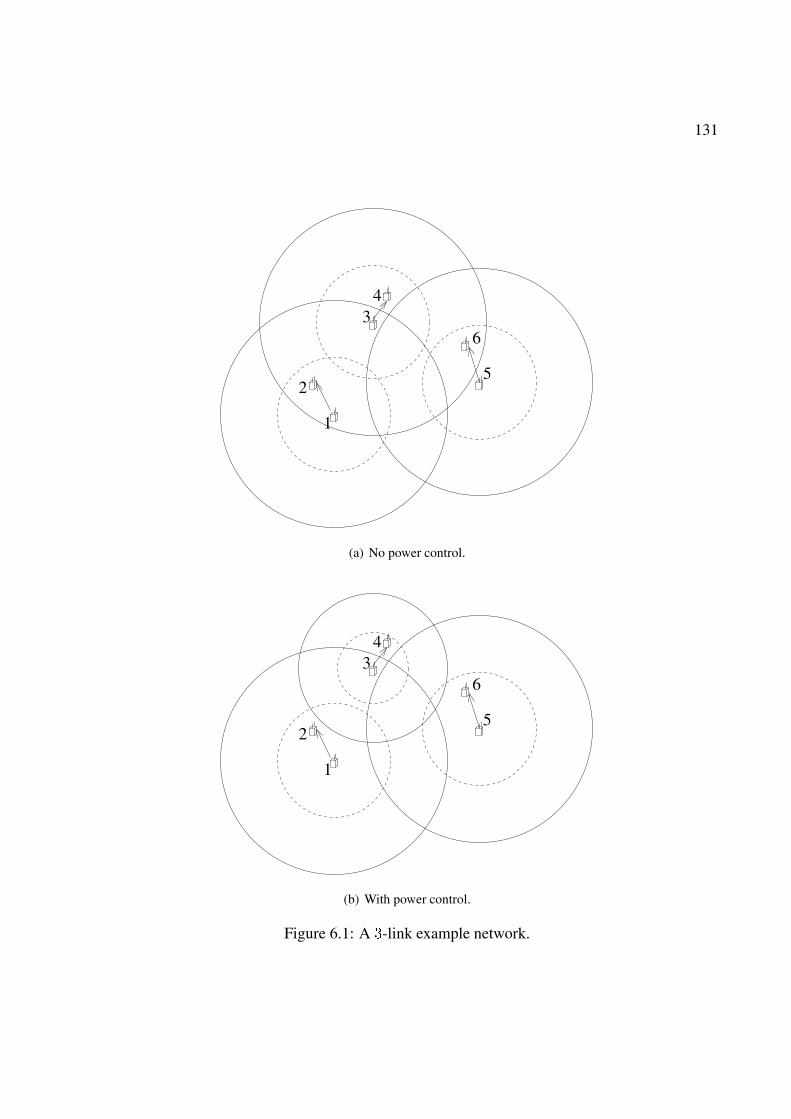
131

4

5

63

2

1

(a) No power control.

4

5

63

2

1

(b) With power control.

Figure 6.1: A -link example network.

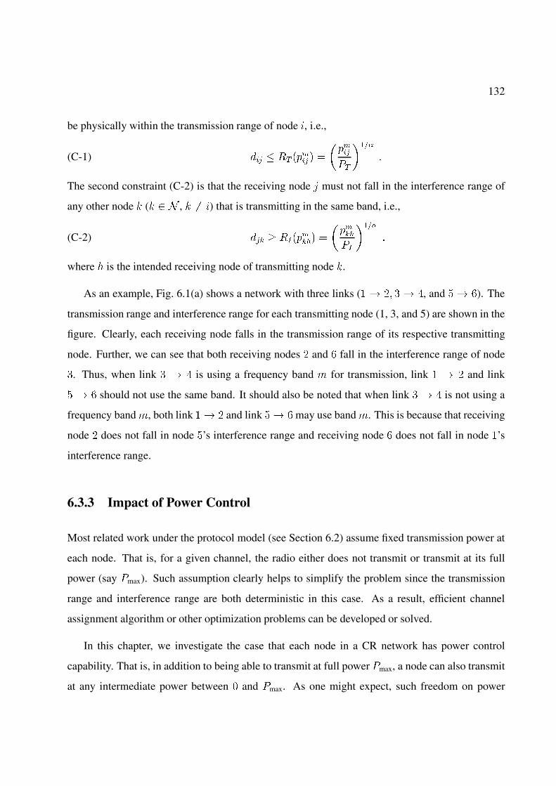
132

be physically within the transmission range of node , i.e.,

(C-1) ��

��7�

��

�

The second constraint (C-2) is that the receiving node ' must not fall in the interference range of

any other node � (� � , � �� ) that is transmitting in the same band, i.e.,

(C-2) ��

��7�

��

�

where � is the intended receiving node of transmitting node �.

As an example, Fig. 6.1(a) shows a network with three links (� � �� , and � � �). The

transmission range and interference range for each transmitting node (1, 3, and 5) are shown in the

figure. Clearly, each receiving node falls in the transmission range of its respective transmitting

node. Further, we can see that both receiving nodes � and � fall in the interference range of node

. Thus, when link � � is using a frequency band ! for transmission, link � � � and link

� � � should not use the same band. It should also be noted that when link � � is not using a

frequency band !, both link �� and link �� may use band !. This is because that receiving

node � does not fall in node �’s interference range and receiving node � does not fall in node �’s

interference range.

6.3.3 Impact of Power Control

Most related work under the protocol model (see Section 6.2) assume fixed transmission power at

each node. That is, for a given channel, the radio either does not transmit or transmit at its full

power (say 7max). Such assumption clearly helps to simplify the problem since the transmission

range and interference range are both deterministic in this case. As a result, efficient channel

assignment algorithm or other optimization problems can be developed or solved.

In this chapter, we investigate the case that each node in a CR network has power control

capability. That is, in addition to being able to transmit at full power 7max, a node can also transmit

at any intermediate power between � and 7max. As one might expect, such freedom on power

133

control has significant impact on design space. In the rest of this section, we illustrate the impact

of power control on scheduling feasibility, bandwidth efficiency, and problem complexity.

Scheduling Feasibility. Constraint (C-2) says that a receiving node ' (corresponding to trans-

mitting node on band !) must not fall in the interference range of any other transmitting node �

that is transmitting in the same band. In the absence of power control, the interference ranges for

all the nodes in the network are fixed and there is hardly much we can do once we encounter an

infeasibility scenario in scheduling. On the other hand, when power control capability is available,

we could adjust the transmission power and thus reduce the interference range of some node so as

to achieve scheduling feasibility.

We use an example to illustrate this important point. Recall that in Fig. 6.1(a), where there

is no power control (and thus the transmission ranges and interference ranges for transmitting

nodes �, , and � are deterministic and shown in the figure), once link � � is active (i.e., in

transmission) in a frequency band !, then neither link � � � nor link � � � shall be active in

the same frequency band. If frequency band ! is the only band available for these links, then it

is impossible to schedule transmissions on links � � � and � � �. Now consider that each node

has the power control capability and can adjust transmission power anywhere in �� 7max�. In this

setting, node could reduce its transmission power while still maintaining data transmission to

node � (see Fig. 6.1(b)). Now receiving nodes � and � are no longer in node ’s interference range.

As a result of this, both transmitting nodes � and � can transmit in the same frequency band !

simultaneously. In other words, power control could enable scheduling feasibility.

Bandwidth Efficiency. Power control capability has the additional benefit of reducing spectrum

bandwidth requirement in the network. This is a direct consequence of the scheduling feasibility

benefit discussed above.

Continuing the previous example, in Fig. 6.1(a), when there is no power control, one frequency

band is inadequate to support all three links and we need at least two frequency bands in the

network. However, when there is power control, in Fig. 6.1(b), we only need one frequency band to

support all three links. In general, one should expect once power control is employed, the spectrum

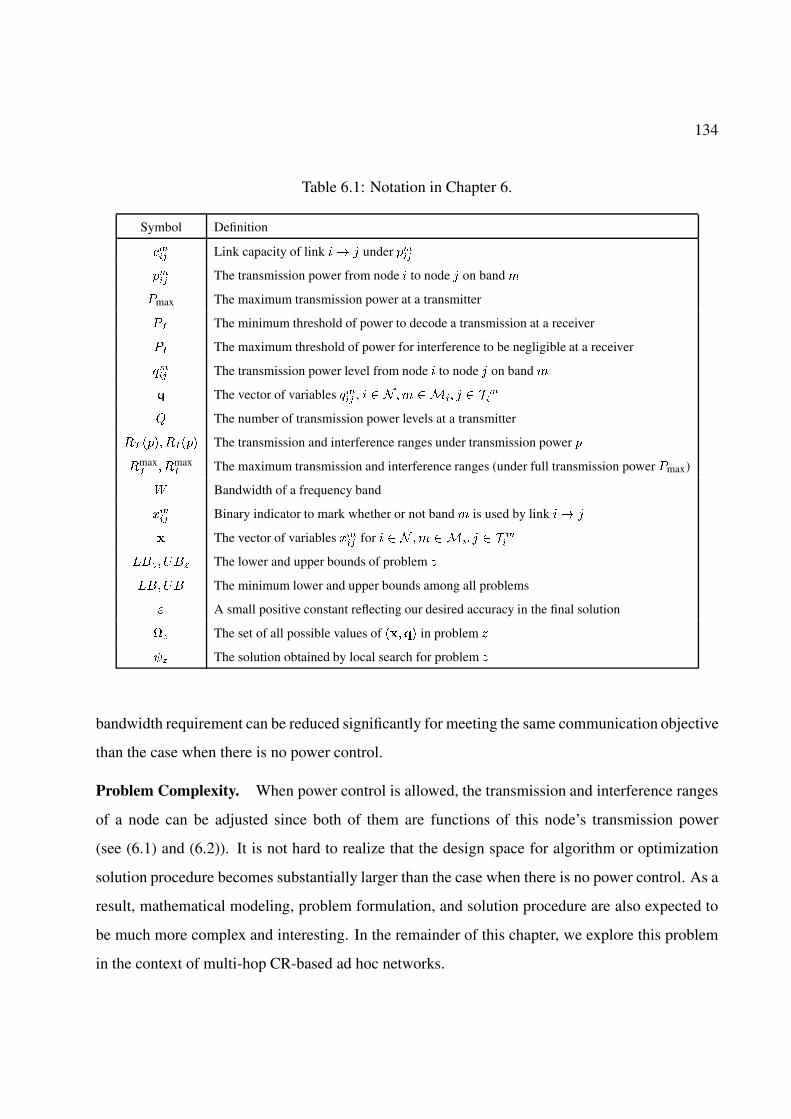
134


Symbol Definition

,�� Link capacity of link �� under ��

�� The transmission power from node � to node � on band �

-max The maximum transmission power at a transmitter

-� The minimum threshold of power to decode a transmission at a receiver

- The maximum threshold of power for interference to be negligible at a receiver

.�� The transmission power level from node � to node � on band �

� The vector of variables .�� , � � � ��

) The number of transmission power levels at a transmitter

� �� The transmission and interference ranges under transmission power �

max� � max

The maximum transmission and interference ranges (under full transmission power -max)

$ Bandwidth of a frequency band

&�� Binary indicator to mark whether or not band � is used by link ��

� The vector of variables &�� for � � � ��

�� /�� The lower and upper bounds of problem 0

��/� The minimum lower and upper bounds among all problems

� A small positive constant reflecting our desired accuracy in the final solution

�� The set of all possible values of �� in problem 0

�� The solution obtained by local search for problem 0

bandwidth requirement can be reduced significantly for meeting the same communication objective

than the case when there is no power control.

Problem Complexity. When power control is allowed, the transmission and interference ranges

of a node can be adjusted since both of them are functions of this node’s transmission power

(see (6.1) and (6.2)). It is not hard to realize that the design space for algorithm or optimization

solution procedure becomes substantially larger than the case when there is no power control. As a

result, mathematical modeling, problem formulation, and solution procedure are also expected to

be much more complex and interesting. In the remainder of this chapter, we explore this problem

in the context of multi-hop CR-based ad hoc networks.

135

6.4 Mathematical Modeling

We consider an ad hoc network consisting of a set � of nodes. Unlike MC-MR networks where

the set of available frequency bands at each node is identical, in a CR network, the set of available

frequency bands at each node depends on its location and may not be the same. For example, at

node , its available frequency bands may consist of bands I, III, and V while at a different node

', its available frequency bands may consist of bands I, IV, and VI, and so forth. More formally,

denote�� the set of available frequency bands at node . For simplicity, we assume the bandwidth

of each frequency band is 0 .1 Denote � the set of all frequency bands present in the network,

i.e., � ��

�� . Table 6.1 lists all notation that are used only in this chapter.

6.4.1 Scheduling and Power Control

In Section 6.3, we discussed the necessary and sufficient condition for successful transmission and

impact of power control on scheduling feasibility. In this section, we formalize these ideas into a

mathematical model in the general context of multi-hop CR networks.

Suppose that band ! is available at both node and node ', i.e., ! ��, where ��

��

�. Denote

��

!"# � If node transmits data to node ' on frequency band !,

� otherwise.

As mentioned earlier, we consider scheduling in the frequency domain and thus once a band !

�� is used by node for transmission to node ', this band cannot be used again by node to

transmit to a different node. That is,

(C-3)��

�

��

where � �� is the set of nodes that are within the transmission range from node under full power

7max on band !.1The case of heterogeneous bandwidth for each frequency band can be easily extended.

136

Denote �max� the maximum transmission range of a node when it transmits at full power 7max.

Then based on (6.1), we have

�max� � �� 7max� �

�7max

7�

��

�

Thus, we have

7� �7max

��max� ��

�

Then for a node transmitting at a power �� 7max�, its transmission range is

��

�

7�

��

�

��max

� ��

7max

��

�

�

7max

��

�max� � (6.3)

Similarly, denote �max� the maximum interference range of a node when it transmits at full power

7max. Then following the same token, we have

�max� � ��7max� �

�7max

7�

��

7� �7max

��max� ��

�

For a node transmitting at a power �� 7max�, its interference range is

��

�

7max

��

�max� � (6.4)

Recall that � �� denotes the set of nodes that are within the transmission range from node under

full power 7max on band !. More formally, we have � �� ' � �� max

� � ' �� ! ��.

Similarly, denote �� the set of nodes that can make interference on node ' on band ! under full

power 7max, i.e., �� max� � � �

� �� . The physical meaning of � �� in the above

definition for �� is that the interfering node � can use band ! for a valid transmission to a node

in � �� .

Note that the definitions of � �� and �� are both based on full transmission power 7max.

When power level is below 7max, the corresponding transmission and interference ranges will

be smaller. As a result, it is necessary to keep track of the set of nodes fall in the transmission

137

range and the set of nodes that can produce interference whenever transmission power changes at

a node.

Recall the two constraints (C-1) and (C-2) for successful transmission from node to node '

and (6.3) and (6.4), respectively, we have

��

��7max

��

�max� (6.5)

��

��7max

��

�max� ��

� � � (6.6)

Based on (6.5) and (6.6), we have the following requirements for the transmission link � '

and interfering link � � �:

��

!"#

��

�max�

��7max� 7max

If �� ,

� � If �� .

��

!"#�

��max

��7max If �� ,

7max If �� .��

� � �

Mathematically, these requirements can be re-written as

(C-1’) ��

&��max

�

��

7max�� 7max�

��

'

(C-2’) �� 7max �

��

��max

�

��7max�

��

� � �

Recall that we consider scheduling in the frequency domain and in (C-3), we state that once

a band ! is used by node for transmission to node ', this band cannot be used again by node

to transmit to a different node. In addition, for successful scheduling in frequency domain, the

following two constraints must also hold.

(C-4) For a band ! � that is available at node ', this band cannot be used for both transmis-

sion and receiving. That is, if band ! is used at node ' for transmission (or receiving), then

it cannot be used for receiving (or transmission).

138

(C-5) Similar to constraint (C-3) on transmission, node ' cannot use the same band ! � for

receiving from multiple nodes.

Note that (C-4) can be viewed as “self-interference” avoidance constraint where at the same

node ', its transmission to another node � on band ! interferes its reception from node in the

same band. It turns out that the above two constraints are mathematically embedded in (C-1’) and

(C-2’). That is, once (C-1’) and (C-2’) are satisfied, then both constraints (C-4) and (C-5) are also

satisfied. This result is formally stated in the following lemma.

Lemma 8. If transmission powers on every transmission link and interference link satisfy (C-1’)

and (C-2’) in the network, then (C-4) and (C-5) are also satisfied.

Proof. We first prove that (C-1’) and (C-2’) leads to (C-4).

� To show that (C-1’) and (C-2’) lead to (C-4), we first let � � ' in (C-2’). Then (C-2’)

degenerates into �� 7max � 7max�� since � � �. If node ' is receiving from node on

band !, i.e., �� , then �� 7max � 7max�� . Since ��

� ��max�

�#7max�

�� in

(C-1’), we have that �� must be �. That is, if node ' is receiving from node on band !,

then node ' cannot transmit to a node � in the same band.

� Now suppose node ' is transmitting to node � on band !, i.e., �� . We will show that

this will lead to �� . This can be proved by contradiction. That is, if �� , then

we have just proved in the above paragraph that �� . But this contradicts our initial

assumption that �� . Therefore, �� must be �. That is, if node ' is transmitting to node

� on band !, then node ' cannot use the same band for receiving from a node .

Combining the above two results, we have shown that (C-4) holds.

We now prove that (C-1’) and (C-2’) also leads to (C-5). Again the proof is based on contra-

diction. Suppose that (C-5) does not hold. Then node ' can receive from two different nodes

and � on the same band !, i.e., �� and �� . Note that link � � ' can be viewed as an

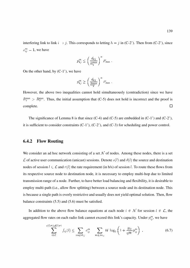
139

interfering link to link � '. This corresponds to letting � � ' in (C-2’). Then from (C-2’), since

�� , we have

��

��max

�

��

7max �

On the other hand, by (C-1’), we have

��

��max

�

��

7max �

However, the above two inequalities cannot hold simultaneously (contradiction) since we have

�max� � �max

� . Thus, the initial assumption that (C-5) does not hold is incorrect and the proof is

complete.

The significance of Lemma 8 is that since (C-4) and (C-5) are embedded in (C-1’) and (C-2’),

it is sufficient to consider constraints (C-1’), (C-2’), and (C-3) for scheduling and power control.

6.4.2 Flow Routing

We consider an ad hoc network consisting of a set � of nodes. Among these nodes, there is a set

� of active user communication (unicast) sessions. Denote 2�� and �� the source and destination

nodes of session � � and �� the rate requirement (in b/s) of session �. To route these flows from

its respective source node to destination node, it is necessary to employ multi-hop due to limited

transmission range of a node. Further, to have better load balancing and flexibility, it is desirable to

employ multi-path (i.e., allow flow splitting) between a source node and its destination node. This

is because a single path is overly restrictive and usually does not yield optimal solution. Then, flow

balance constraints (5.5) and (5.6) must be satisfied.

In addition to the above flow balance equations at each node � for session � �, the

aggregated flow rates on each radio link cannot exceed this link’s capacity. Under �� , we have

��

��

��

��

��

0 ��

��

$�50

��

�� (6.7)

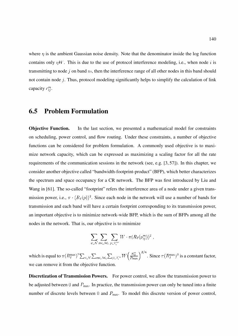
140

where 5 is the ambient Gaussian noise density. Note that the denominator inside the log function

contains only 50 . This is due to the use of protocol interference modeling, i.e., when node is

transmitting to node ' on band !, then the interference range of all other nodes in this band should

not contain node '. Thus, protocol modeling significantly helps to simplify the calculation of link

capacity �� .

6.5 Problem Formulation

Objective Function. In the last section, we presented a mathematical model for constraints

on scheduling, power control, and flow routing. Under these constraints, a number of objective

functions can be considered for problem formulation. A commonly used objective is to maxi-

mize network capacity, which can be expressed as maximizing a scaling factor for all the rate

requirements of the communication sessions in the network (see, e.g. [3, 57]). In this chapter, we

consider another objective called “bandwidth-footprint-product” (BFP), which better characterizes

the spectrum and space occupancy for a CR network. The BFP was first introduced by Liu and

Wang in [61]. The so-called “footprint” refers the interference area of a node under a given trans-

mission power, i.e., / � ��. Since each node in the network will use a number of bands for

transmission and each band will have a certain footprint corresponding to its transmission power,

an important objective is to minimize network-wide BFP, which is the sum of BFPs among all the

nodes in the network. That is, our objective is to minimize

��

��

��

�

0 � /��

� �

which is equal to /��max� ��

��

��

��

�0�

��$max

��#. Since /��max

� �� is a constant factor,

we can remove it from the objective function.

Discretization of Transmission Powers. For power control, we allow the transmission power to

be adjusted between � and 7max. In practice, the transmission power can only be tuned into a finite

number of discrete levels between � and 7max. To model this discrete version of power control,

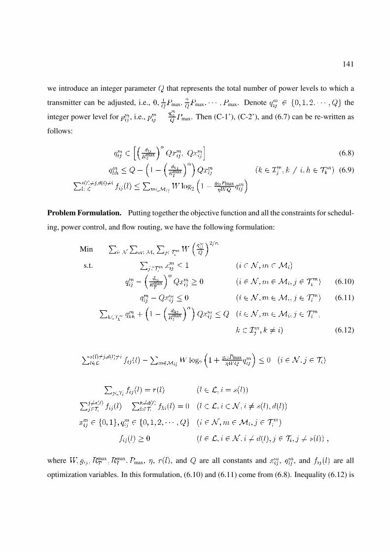
141

we introduce an integer parameter 4 that represents the total number of power levels to which a

transmitter can be adjusted, i.e., �� !7max�

�!7max� � � � � 7max. Denote �� 4� the

integer power level for �� , i.e., �� !7max. Then (C-1’), (C-2’), and (6.7) can be re-written as

follows:

��

��max�

��4�� 4��

(6.8)

�� 4��

� ��max

��4��

� � (6.9)��

��

0 ��

��

��$max"�!

��

�

Problem Formulation. Putting together the objective function and all the constraints for schedul-

ing, power control, and flow routing, we have the following formulation:

Min�

��

��

��

�0��!

��s.t.

��

�� ! ��

��

��max�

��4�� ! �� ' �

�� (6.10)

�� 4�� ! �� ' �� (6.11)�

��

��

� ��max

��4�� 4 � � � ! �� ' �

��

� �� (6.12)

��

��

0 ��

�� $max

"�! ��

�� ' ��

��

�� 2��

��

�� 2��

�� 4� � � � ! �� ' �

��

�� ' �� ' �� 2��

where 0� $�� max� � �max

� � 7max, 5, ��, and 4 are all constants and �� , �� , and �� are all

optimization variables. In this formulation, (6.10) and (6.11) come from (6.8). Inequality (6.12) is

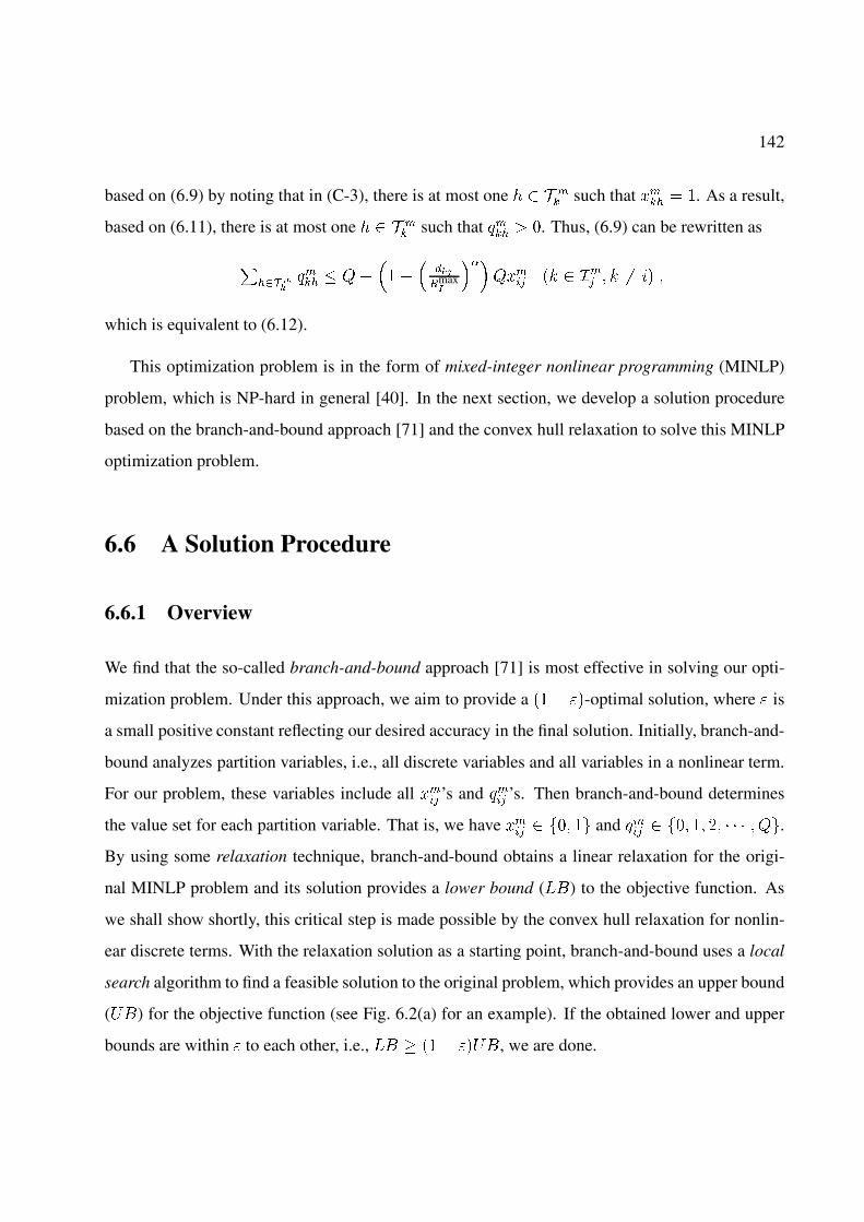
142

based on (6.9) by noting that in (C-3), there is at most one � � �� such that �� . As a result,

based on (6.11), there is at most one � � �� such that �� . Thus, (6.9) can be rewritten as

��

� �� 4�

��

� ��max

��4��

which is equivalent to (6.12).

This optimization problem is in the form of mixed-integer nonlinear programming (MINLP)

problem, which is NP-hard in general [40]. In the next section, we develop a solution procedure

based on the branch-and-bound approach [71] and the convex hull relaxation to solve this MINLP

optimization problem.

6.6 A Solution Procedure

6.6.1 Overview

We find that the so-called branch-and-bound approach [71] is most effective in solving our opti-

mization problem. Under this approach, we aim to provide a �� -optimal solution, where � is

a small positive constant reflecting our desired accuracy in the final solution. Initially, branch-and-

bound analyzes partition variables, i.e., all discrete variables and all variables in a nonlinear term.

For our problem, these variables include all �� ’s and �� ’s. Then branch-and-bound determines

the value set for each partition variable. That is, we have �� and �� 4�.

By using some relaxation technique, branch-and-bound obtains a linear relaxation for the origi-

nal MINLP problem and its solution provides a lower bound (�() to the objective function. As

we shall show shortly, this critical step is made possible by the convex hull relaxation for nonlin-

ear discrete terms. With the relaxation solution as a starting point, branch-and-bound uses a local

search algorithm to find a feasible solution to the original problem, which provides an upper bound

(8() for the objective function (see Fig. 6.2(a) for an example). If the obtained lower and upper

bounds are within � to each other, i.e., �( �� 8(, we are done.

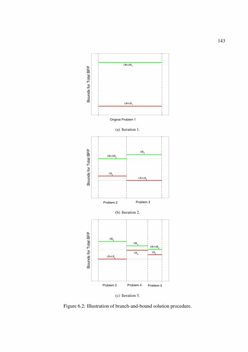
143

Bou

nds

for

Tot

al B

FP

Original Problem 1

LB=LB1

UB=UB1

(a) Iteration 1.

Bou

nds

for

Tot

al B

FP

Problem 2 Problem 3

LB2

UB3

UB=UB2

LB=LB3

(b) Iteration 2.

Bou

nds

for

Tot

al B

FP

Problem 2 Problem 4 Problem 5

LB=LB2

LB5LB

4

UB2

UB4

UB=UB5

(c) Iteration 3.

Figure 6.2: Illustration of branch-and-bound solution procedure.

144

Branch-and-bound Procedure

1. Initialization:

2. Let the initial best solution �� and the initial upper bound � ��.

3. Determine initial value set for each partition variable.

4. Let the initial problem list include only the original problem, denoted as problem �.

5. Build a linear relaxation and obtain the relaxation solution ��.

6. The objective value of �� is a lower bound �� to problem �.

7. Iteration:

8. Suppose problem � has the minimum ��% among all problems in the problem list.

9. Update lower bound �� % .

10. Find a feasible solution �% from �% via a local search algorithm and denote its objective value

11. as �% .

12. If ( �% � �) �

13. Update �� % and � � �% .

14. If �� , we stop with the �� -optimal solution ��.

15. Otherwise, remove all problems �� with ��%� �� from the problem list. �

16. Select a variable with the maximum relaxation error and divide its value set into two sets by

17. its value in �% .

18. Build two new problems �� and �� based on these two sets.

19. Remove problem � from the problem list.

20. Obtain ��%� and ��%� for problems �� and �� via their linear relaxations.

21. If ��%� � �� , add problem �� into the problem list.

22. If ��%� � �� , add problem �� into the problem list.

23. If the problem list is empty, we stop with the �� -optimal solution ��.

24. Otherwise, go to the next iteration.

Figure 6.3: A general framework of the branch-and-bound solution procedure.

145

If the relaxation errors for nonlinear terms are not small, then the upper bound 8( could be far

away from the lower bound �(. To close this gap, we must have a tighter linear relaxation, i.e.,

with smaller relaxation errors. This could be achieved by further narrowing down the value sets of

partition variables. Specifically, branch-and-bound selects a partition variable with the maximum

relaxation error and divides its value set into two sets by its value in the relaxation solution (see

Fig. 6.2(b)). Then the original problem (denoted as problem �) is divided into two new problems

(denoted as problem � and problem ). Again, branch-and-bound performs relaxation and local

search on these two new problems. Now we have lower bounds �(� and �( for problems � and ,

respectively. We also have feasible solutions that provide upper bounds 8(� and 8( for problems

� and , respectively. Since the relaxations in problems � and are both tighter than that in problem

�, we have ��8(�� 8(� � 8(� and �(�� ( �(�. For a minimization problem, the

lower bound of the original problem is updated from �( � �(� to �( � ��(�� (�. Also,

the best feasible solution to the original problem is the solution with a smaller 8(�. Then the

upper bound of the original problem is updated from 8( � 8(� to 8( � ��8(�� 8(�.

As a result, we now have smaller gap between 8( and �(. If �( �� 8(, we are done.

Otherwise, we choose a problem with the minimum lower bound (Problem in Fig. 6.2(b)) and

perform partition for this problem.

Note that during the iteration process for branch-and-bound, if we find a problem 9 with �(%

��8(, then we can conclude that this problem cannot provide much improvement on 8( (see

problem � in Fig. 6.2(c)). That is, further branch on this problem will not yield much improvement

and we can thus remove this problem from further consideration. Eventually, once we find �(

�� 8(, branch-and-bound procedure terminates. It has been shown that under very general

conditions, a branch-and-bound solution procedure always converges [89]. Moreover, although the

worst-case complexity of such a procedure is exponential, the actual running time could be fast if

all partition variables are integer variables (e.g., the problem considered in this chapter).

Figure 6.3 shows the general framework of branch-and-bound procedure. Several key com-

ponents in the branch-and-bound procedure are problem specific and remain to be solved. These

include

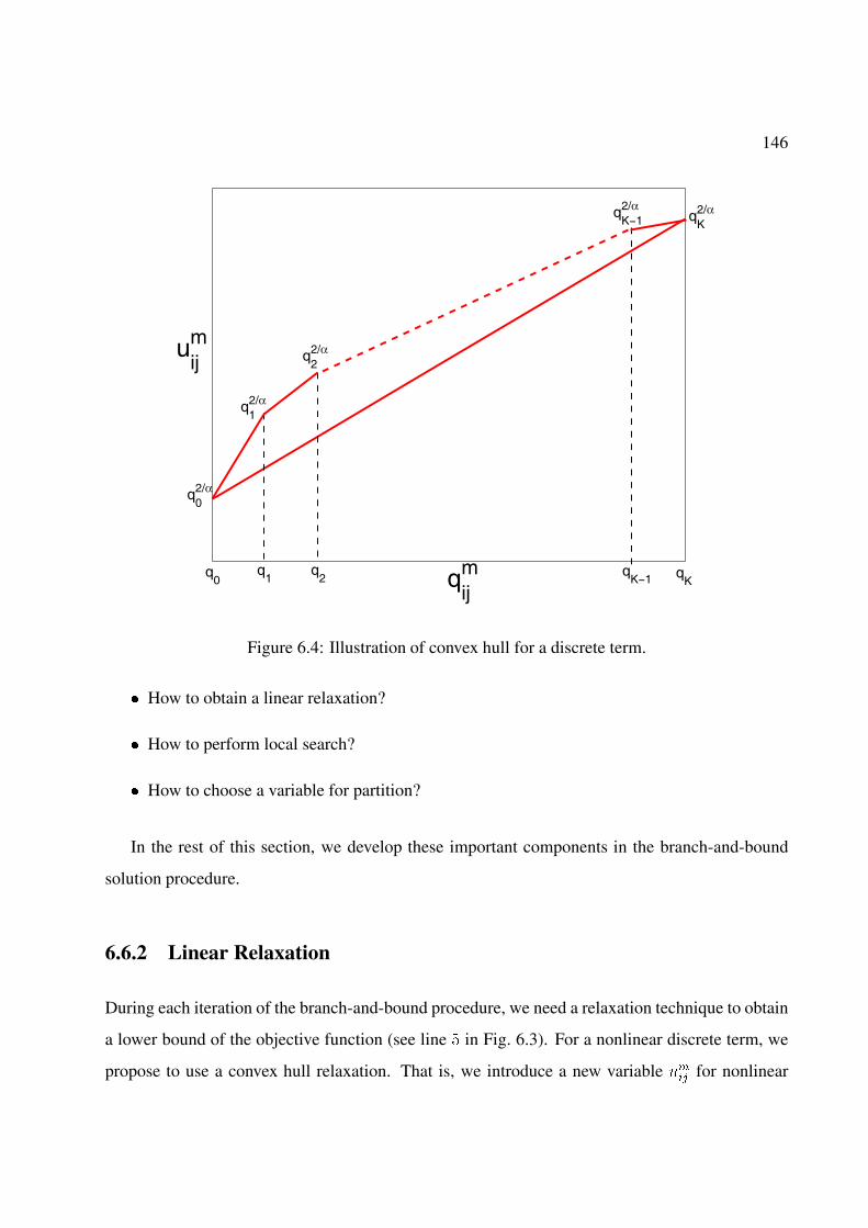
146

qijm

uijm

q0 q

K

q02/α

q1 q

2 qK−1

q12/α

q22/α

qK−12/α

qK2/α

Figure 6.4: Illustration of convex hull for a discrete term.

� How to obtain a linear relaxation?

� How to perform local search?

� How to choose a variable for partition?

In the rest of this section, we develop these important components in the branch-and-bound

solution procedure.

6.6.2 Linear Relaxation

During each iteration of the branch-and-bound procedure, we need a relaxation technique to obtain

a lower bound of the objective function (see line � in Fig. 6.3). For a nonlinear discrete term, we

propose to use a convex hull relaxation. That is, we introduce a new variable 6�� for nonlinear

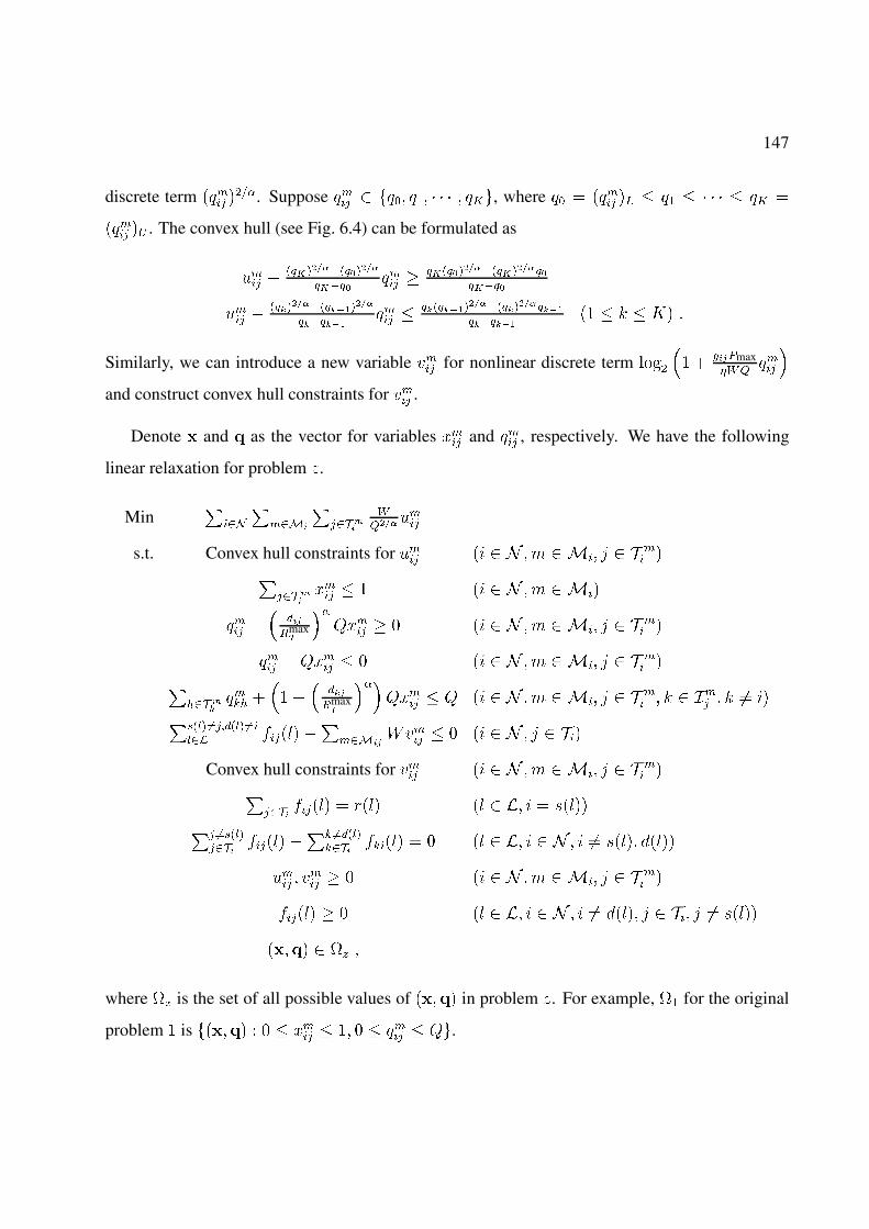
147

discrete term � �� . Suppose �� , where � � � ��

� �� & . The convex hull (see Fig. 6.4) can be formulated as

6��

��

��

��

6��

��

��

��

��

��

�� .� �

Similarly, we can introduce a new variable �� for nonlinear discrete term ��

�� $max

"�! ��

�and construct convex hull constraints for �� .

Denote � and � as the vector for variables �� and �� , respectively. We have the following

linear relaxation for problem 9.

Min�

��

��

��

�!�� 6

��

s.t. Convex hull constraints for 6�� ! �� ' �

��

�� ! ��

��

��max�

��4�� ! �� ' �

��

�� 4�� ! �� ' ��

��

��

� ��max

��4�� 4 � � � ! �� ' �

��

��

�� 0�� ' ��

Convex hull constraints for �� ! �� ' ��

�� 2��

��

��

�� 2��

6��

�� ! �� ' �

��

�� ' �� ' �� 2��

�� % �

where �% is the set of all possible values of �� in problem 9. For example, �� for the original

problem � is �� 4�.

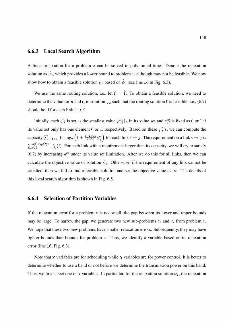
148

6.6.3 Local Search Algorithm

A linear relaxation for a problem 9 can be solved in polynomial time. Denote the relaxation

solution as �-%, which provides a lower bound to problem 9, although may not be feasible. We now

show how to obtain a feasible solution -% based on �-% (see line �� in Fig. 6.3).

We use the same routing solution, i.e., let � � �� . To obtain a feasible solution, we need to

determine the value for � and � in solution -% such that the routing solution � is feasible, i.e., (6.7)

should hold for each link � '.

Initially, each �� is set as the smallest value � �� in its value set and �� is fixed as � or � if

its value set only has one element � or �, respectively. Based on these �� ’s, we can compute the

capacity�

�� 0 ��

�� $max

"�! ��

�for each link � '. The requirement on a link � ' is��

�� . For each link with a requirement larger than its capacity, we will try to satisfy

(6.7) by increasing �� under its value set limitation. After we do this for all links, then we can

calculate the objective value of solution -% . Otherwise, if the requirement of any link cannot be

satisfied, then we fail to find a feasible solution and set the objective value as �. The details of

this local search algorithm is shown in Fig. 6.5.

6.6.4 Selection of Partition Variables

If the relaxation error for a problem 9 is not small, the gap between its lower and upper bounds

may be large. To narrow the gap, we generate two new sub-problems 9� and 9� from problem 9.

We hope that these two new problems have smaller relaxation errors. Subsequently, they may have

tighter bounds than bounds for problem 9. Thus, we identify a variable based on its relaxation

error (line ��, Fig. 6.3).

Note that � variables are for scheduling while � variables are for power control. It is better to

determine whether to use a band or not before we determine the transmission power on this band.

Thus, we first select one of � variables. In particular, for the relaxation solution �-%, the relaxation

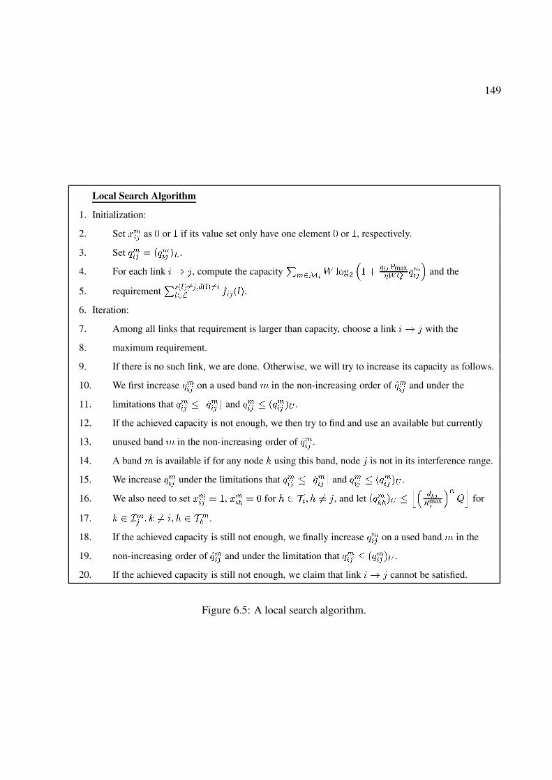
149

Local Search Algorithm

1. Initialization:

2. Set �� as � or � if its value set only have one element � or �, respectively.

3. Set �� .

4. For each link �� , compute the capacity�

��

��

��$max"�! ��

and the

5. requirement��

�� .

6. Iteration:

7. Among all links that requirement is larger than capacity, choose a link �� with the

8. maximum requirement.

9. If there is no such link, we are done. Otherwise, we will try to increase its capacity as follows.

10. We first increase �� on a used band � in the non-increasing order of �� and under the

11. limitations that �� and �� & .

12. If the achieved capacity is not enough, we then try to find and use an available but currently

13. unused band � in the non-increasing order of �� .

14. A band � is available if for any node � using this band, node is not in its interference range.

15. We increase �� under the limitations that �� and �� & .

16. We also need to set �� , �� for � � �� , and let ��& ��

��max

��

for

17. � � �� .

18. If the achieved capacity is still not enough, we finally increase �� on a used band � in the

19. non-increasing order of �� and under the limitation that �� & .

20. If the achieved capacity is still not enough, we claim that link �� cannot be satisfied.

Figure 6.5: A local search algorithm.

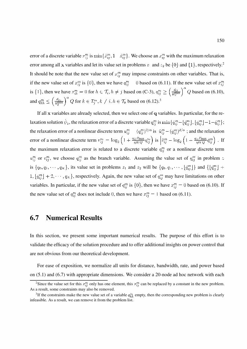
150

error of a discrete variable �� is �� . We choose an �� with the maximum relaxation

error among all � variables and let its value set in problems 9� and 9� be �� and ��, respectively.2

It should be note that the new value set of �� may impose constraints on other variables. That is,

if the new value set of �� is ��, then we have �� based on (6.11). If the new value set of ��

is ��, then we have �� for � �� ' based on (C-3), ��

��max�

��4 based on (6.10),

and ��

��max

��4 for � �� based on (6.12).3

If all � variables are already selected, then we select one of � variables. In particular, for the re-

laxation solution �-% , the relaxation error of a discrete variable �� is ��

�� ;

the relaxation error of a nonlinear discrete term 6��

�� is �6��

�� ; and the relaxation

error of a nonlinear discrete term ��

�� $max

"�! ��

�is(((��

�� $max

"�!� ��

�(((. If

the maximum relaxation error is related to a discrete variable �� or a nonlinear discrete term

6�� or �� , we choose �� as the branch variable. Assuming the value set of �� in problem 9

is � �� , its value set in problems 9� and 9� will be � �� and ��

�� , respectively. Again, the new value set of �� may have limitations on other

variables. In particular, if the new value set of �� is ��, then we have �� based on (6.10). If

the new value set of �� does not include �, then we have �� based on (6.11).

6.7 Numerical Results

In this section, we present some important numerical results. The purpose of this effort is to

validate the efficacy of the solution procedure and to offer additional insights on power control that

are not obvious from our theoretical development.

For ease of exposition, we normalize all units for distance, bandwidth, rate, and power based

on (5.1) and (6.7) with appropriate dimensions. We consider a 20-node ad hoc network with each

2Since the value set for this &�� only has one element, this &�� can be replaced by a constant in the new problem.As a result, some constraints may also be removed.

3If the constraints make the new value set of a variable .�� empty, then the corresponding new problem is clearlyinfeasible. As a result, we can remove it from the problem list.

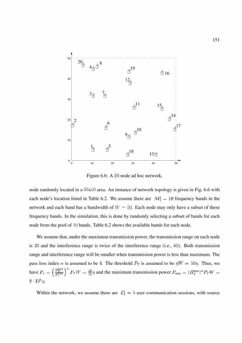
151

4

00

10

20

40

50

30

10 20 30 40 50

3

8

6

518

9

11

10

1612

1920

7

13

15

14

17

1

2

Figure 6.6: A ��-node ad hoc network.

node randomly located in a ��x�� area. An instance of network topology is given in Fig. 6.6 with

each node’s location listed in Table 6.2. We assume there are � � �� frequency bands in the

network and each band has a bandwidth of 0 � ��. Each node may only have a subset of these

frequency bands. In the simulation, this is done by randomly selecting a subset of bands for each

node from the pool of �� bands. Table 6.2 shows the available bands for each node.

We assume that, under the maximum transmission power, the transmission range on each node

is �� and the interference range is twice of the interference range (i.e., ��). Both transmission

range and interference range will be smaller when transmission power is less than maximum. The

pass loss index � is assumed to be �. The threshold 7� is assumed to be 50 � ��5. Thus, we

have 7� ��max�

�max

��7�0 � �

��5 and the maximum transmission power 7max � ��max

� ��7�0 �

� � ��5.

Within the network, we assume there are � � � user communication sessions, with source

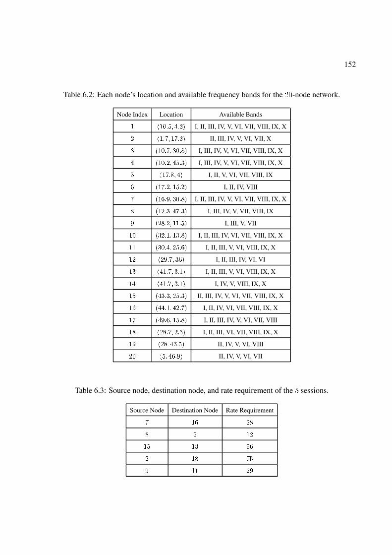
152

Table 6.2: Each node’s location and available frequency bands for the ��-node network.

Node Index Location Available Bands

� ��#�� #�� I, II, III, IV, V, VI, VII, VIII, IX, X

��#�� #�� II, III, IV, V, VI, VII, X

� ��#�� #�� I, III, IV, V, VI, VII, VIII, IX, X

� ��#� ��#�� I, III, IV, V, VI, VII, VIII, IX, X

� ��#�� I, II, V, VI, VII, VIII, IX

� ��#� ��#� I, II, IV, VIII

� ��#�� #�� I, II, III, IV, V, VI, VII, VIII, IX, X

� ��#�� #�� I, III, IV, V, VII, VIII, IX

� ��#� ��#�� I, III, V, VII

�� #�� #�� I, II, III, IV, VI, VII, VIII, IX, X

�� #�� #�� I, II, III, V, VI, VIII, IX, X

� ��#�� I, II, III, IV, VI, VI

�� #�� #�� I, II, III, V, VI, VIII, IX, X

�� #�� #�� I, IV, V, VIII, IX, X

�� #�� #�� II, III, IV, V, VI, VII, VIII, IX, X

�� #�� #�� I, II, IV, VI, VII, VIII, IX, X

�� #�� #�� I, II, III, IV, V, VI, VII, VIII

�� #�� #�� I, II, III, VI, VII, VIII, IX, X

�� #�� II, IV, V, VI, VIII

� �� #�� II, IV, V, VI, VII

Table 6.3: Source node, destination node, and rate requirement of the � sessions.

Source Node Destination Node Rate Requirement

� ��

� � �

��

��

� ��

153

1 3 5 7 9 11 13 150

100

200

300

400

500

600

Q

Tot

al C

ost

Figure 6.7: Total cost as a function of discretization levels of power control.

node and destination node randomly selected and the rate of each session is randomly generated

within �� . Table 6.3 specifies an instance of the source node, destination node, and rate

requirement for the 5 sessions in the network.

We set the desired approximation error bound � to be �� in the solution procedure (Sec-

tion 6.6), which guarantees that the obtained solution is within �% from the optimum.

6.7.1 Power Control and Level of Granularity on BFP

In this set of numerical results, we apply the solution procedure to the 20-node network described

above for different level of power control granularity (4). Note that 4 � � corresponds to the

case that there is no power control, i.e., a node uses its peak power 7max for transmission. When

4 is sufficiently large, the discrete nature of power control diminishes and power control becomes

continuous between �� 7max�.

Figure 6.7 shows the results from our solution procedure. First, we note that power control has a

significant impact on BFP. Comparing the case when there is no power control (4 � �) and the case

154

of 4 � ��, we find that there is nearly a ��% reduction in the total cost (objective value). Second,

the cost (objective) is a non-increasing function of 4. However, when 4 becomes sufficiently

large (e.g., �� in this network setting), further increase in 4 will not have much reduction on cost.

This suggests that for practical purpose, the number of required granularity levels to achieve a

reasonably good result does not need to be a large number.

To illustrate the difference in routing under different 4, we record the flow routing topology

for 4 � � (no power control) and 4 � �� in Fig. 6.8 (a) and (b), respectively. In addition to

the obvious difference in flow routing topology starting from node �, we also notice that, due to

power control, the frequency band used on some link in Fig. 6.8(a) and (b) are also different. For

example, in Fig. 6.8(a), we plot the transmission range and interference range for nodes � and ��.

Since there is no power control, node �� has to use the maximum transmission power 7max even

to its neighboring node ��. Since node is in the interference range of node ��, nodes � and ��

cannot use the same frequency band. On the contrary, in Fig. 6.8(b), since each node is capable of

adjusting transmission power (4 � ��), both nodes � and node �� can use smaller transmission

powers to achieve the same connectivity and bit rates. As a result, in Fig. 6.8(b), node is no

longer in the interference range of node ��. Thus, in the solution to 4 � ��, both nodes � and ��

are allowed to use the same frequency band. This observation from numerical results validate the

benefit on scheduling feasibility brought by power control.

6.7.2 Results on Scheduling Feasibility and Bandwidth Efficiency

To better understand the impact of power control on scheduling feasibility and bandwidth effi-

ciency, we change the available frequency bands in Table 6.2 into the following setting. Each node

in the ��-node network has an identical set of frequency bands, i.e., �� . This special case

is the setting for MC-MR.

Clearly, when � is very small, feasible solution may not exist for either power control case

(4 � ��) or no power control case (4 � �). We now increase the available frequency bands �

155

17

00

10

20

40

50

30

10 20 30 40 50

3

8

1

6

518

9

11

10

1612

1920

2

4

7

13

15

14

(a) No power control () � �)

20

00

10

20

40

50

30

10 20 30 40 50

3

14

5

6

9

12

1710

1

2

4

7

8

11

13

15

16

18

19

(b) With power control () � ��)

Figure 6.8: Routing topology for the � communication sessions in the ��-node network.

156

at each node and find that starting from � � �, we can obtain a feasible solution for the power

control case (4 � ��). However, for � � �, there is still no feasible solution for the no power

control case (4 � �).

It is not hard to see that if we continue to add available frequency bands into the network, we

will eventually have a feasible solution for the no power control case (4 � �). In our numerical

results, we find that only when � � �, we find a first feasible solution for the no power control

case. Recall that we only need � � � for a feasible solution with power control. This example

verifies that not only power control offers greater design space for scheduling feasibility, it also

conserves the number of frequency bands for the network.

6.8 Conclusions

In this chapter, we investigated how to support user communication sessions by jointly perform-

ing power control, scheduling, and flow routing for a CR-based multi-hop wireless network. We

developed a formal mathematical model for scheduling feasibility under the influence of power

control. This model extends the existing so-called protocol model for wireless networks (where

transmission range and interference range are deterministic) and thus can be used for a broad

class of problems where power control (and thus transmission range and interference range) is

part of the optimization space. We formulated a cross-layer optimization problem encompass-

ing power control, scheduling, and flow routing and developed an efficient solution procedure

based on branch-and-bound technique and convex hull relaxation. Through numerical results, we

demonstrated quantitatively that power control and variable transmission/interference range have

significant impact on scheduling feasibility, bandwidth efficiency, and bandwidth-footprint prod-

uct. These results affirm the critical need of incorporating power control under the existing protocol

interference modeling for future wireless network research.

Chapter 7

Summary and Future Work

7.1 Summary

Recently, many new types of wireless networks have emerged for both civil and military applica-

tions. Among these new types of wireless networks, we focus on wireless sensor networks and

ad hoc networks. Wireless sensor networks consist of battery-powered nodes to provide in-situ,

unattended, high-precision, and real-time observation over a vast area. Wireless ad hoc networks

are characterized by the absence of infrastructure support. Nodes in an ad hoc network are able to

self-organize into a multi-hop network.

For these new wireless networks, many advanced physical layer technologies have been de-

veloped to improve performance. In particular, CR has the ability of sensing available bands and

switching among bands. It is enabled by recent advances in RF design, signal processing, and

communication software. CR promises unprecedented flexibility in radio communications and is

viewed as an enabling technology for dynamic spectrum access.

Due to the unique characteristics of these new networks, it is necessary to consider new per-

formance limits, e.g., network lifetime for sensor networks and bandwidth footprint product for

CR networks. Such performance limits are important as they can be used as benchmarks for the

157

158

design of distributed algorithms and protocols. However, due to some unique requirements at the

application layer as well as some unique characteristics associated at the physical layer, existing

analytical approaches developed for traditional wireless networks are not adequate. In this disser-

tation, we focus on the design of new algorithms and optimization techniques to address theoretical

performance limits associated with these new wireless networks.

For these new wireless networks, we find that it is necessary to consider constraints at multiple

layers, e.g., power control at the physical layer, scheduling at the link layer, and routing at the

network layer. The formulation of these problems are usually in very complex form (nonlinear or

non-convex) and are mathematically challenging. In this dissertation, we address these difficult

problems via the development of some novel algorithms that are both efficient and optimal (or

near-optimal). The main contributions of this dissertation are the following.

1. For node lifetime problem, we show how to equitably maximize node lifetime for each

node in a sensor network under the lexicographic max-min (LMM) criteria. We develop a

polynomial-time algorithm based on the parametric analysis (PA) technique, which is com-

putationally more efficient than the slack variable based approach in previous work. In addi-

tion to providing an efficient polynomial-time algorithm for the LMM-optimal node lifetime

vector computation, we also show how to obtain a corresponding routing solution among

the remaining alive nodes at each stage such that the LMM-optimal node lifetime vector

can indeed be achieved. Another contribution of this work is that our approach can also be

employed to address the LMM rate allocation problem, which is similar in structure to the

LMM node lifetime problem. More important, we find a duality relationship between the

LMM node lifetime problem and the LMM rate allocation problem, which enables one to

develop solutions to both problems by solving only one of the two problems.

2. For base station placement problem, we aim to optimally place the base station to maximize

sensor network lifetime. We design a �� -approximation algorithm for this problem,

which is based on subarea division and fictitious cost point (FCP) representation. Under the

given small error bound �, we first divide the infinite search space for base station location

159

into a finite number of subareas. We then represent each subarea by an FCP, which is an � -

tuple cost vector with each component representing the upper bound of cost to a sensor node

in the network. The achievable network lifetime for each FCP can be obtained by a linear

program (LP). We prove that any point in the subarea corresponding the best FCP is a ��-

optimal solution for base station placement. The complexity of our approximation algorithm

is significantly lower than the state-of-the-art algorithm proposed in previous work.

3. For mobile base station problem, we aim to find the optimal base station moving trajectory

as well as time-dependent flow routing solution to maximize lifetime of sensor networks.

We contribute an approximation algorithm regarding the movement of a mobile base station.

The foundation of our result hinges upon a novel time-to-space transformation for problem

formulation. That is, to achieve the maximum network lifetime, we only need to determine

the sojourn time for the base station at each point and the flow routing solution when the base

station is at this point. Based on this transformation, we present an intermediate result which

says that when the location of the base station is constrained to be on a set of pre-determined

points, then the optimal solution can be obtained via an LP. For the general mobile base

station problem where the location of the base station is un-constrained, we transform this

infinite search space into a finite set of FCPs based on the given small error bound �. Then we

can obtain the sojourn time at each FCP (or the corresponding subarea) and the flow routing

solution when base station is at this FCP. We prove that such a solution is �� -optimal.

This is the first theoretical result on mobile base station problem.

4. We consider how to minimize the total required bandwidth in a CR network to support a

given set of communication sessions. For this problem, it is necessary to consider a cross-

layer design, which includes spectrum allocation, scheduling and interference avoidance, and

multi-hop multi-path routing. This problem can be formulated as a mixed integer nonlinear

program (MINLP). To solve this problem, we propose a sequential fixing (SF) procedure to

fix scheduling variables iteratively. Once we have fixed all scheduling variables, the values

to all other variables can be obtained by an LP. Simulation results show that the solutions

160

obtained by SF algorithm are close to a lower bound developed in this work. Thus, these

solutions are even closer to the minimum required bandwidth and are near-optimal.

5. We further consider the case that each CR node has power control capability. That is, in

addition to scheduling and routing, power control is also part of the optimization space. In

this case, we aim to minimize the total required bandwidth footprint product (BFP) to sup-

port a set of user sessions. We follow the so-called protocol model and develop a formal

mathematical model for scheduling with power control. This model extends existing deter-

ministic interference model and can be used for a wide range of problems. Based on this

model, we have formulated a joint power control, scheduling, and routing problem. Our

efficient solution procedure to this cross-layer optimization problem is based on the branch-

and-bound framework and convex hull relaxation. The solution obtained via our approach

yields a �� -optimal solution, where � is a small positive constant reflecting our desired

accuracy in the final solution. This is the first theoretical result on this problem.

7.2 Future Research Direction

The following problems remain open and will be my future research.

� There are two major interference models for wireless networks, i.e., the protocol model (see

Chapters 5 and 6) and the physical model. Under the protocol model, we focus on the

interference relationship between two transmissions, i.e., a receiver is interfered by another

transmitter if the interference from this transmitter cannot be neglected (over a threshold).

Under the physical model, we consider signal to interference plus noise ratio (SINR) directly,

i.e., a receiver is interfered if SINR at this receiver is below a threshold. A common agreed

understanding is that the physical model is more accurate, despite that it is more complex. In

our future work, we will consider how to determine the performance limit under the physical

model via nonlinear optimization techniques. We will explore the relationship between the

physical model and the protocol model. Another question we would like to answer is that

161

whether it is possible to set up a suitable threshold for the protocol model such that it yields

a similar performance to the physical model.

� Distributed algorithms are very important in network implementation. We will consider how

to develop distributed algorithms for the solutions presented in this dissertation. A promising

direction for distributed cross-layer optimization problem is subgradient method [7]. The

essence of this approach is that for these performance limit problems, the subgradient method

may be decomposed into sub-components, each of which is suitable for local computation.

However, if the optimization problem is non-convex, the subgradient method may not be

able to find the global optimal solution. We will explore some innovative ideas based on

subgradient method to provide optimal or near-optimal solutions.

Bibliography

[1] I.F. Akyildiz, W. Su, Y. Sankarasubramaniam, and E. Cayirci, “Wireless sensor networks: Asurvey,” Computer Networks (Elsevier), vol. 38, no. 4, pp. 393–422, 2002.

[2] S.M. Alamouti, “A simple transmit diversity technique for wireless communications,” IEEEJournal on Selected Areas in Communications, vol. 16, issue 8, pp. 1451–1458, Oct. 1998.

[3] M. Alicherry, R. Bhatia, and L. Li, “Joint channel assignment and routing for throughputoptimization in multi-radio wireless mesh networks,” in Proc. ACM Mobicom, pp. 58–72,Cologne, Germany, Aug. 28–Sep. 2, 2005.

[4] BARON Global Optimization Software, http://www.andrew.cmu.edu/user/ns1b/baron/baron.html.

[5] S. Basagni, A. Carosi, E. Melachrinoudis, C. Petrioli, and Z.M. Wang, “A new MILP for-mulation and distributed protocols for wireless sensor networks lifetime maximization,” inProc. IEEE International Conference on Communications, pp. 3517–3524, Istanbul, Turkey,June 11–15, 2006.

[6] M.S. Bazaraa, J.J. Jarvis, and H.D. Sherali, Linear Programming and Network Flows, thirdedition, John Wiley & Sons, 2004.

[7] M.S. Bazaraa, H.D. Sherali, and C.M. Shetty, Nonlinear Programming: Theory and Algo-rithms, third edition, John Wiley & Sons, Inc., New York, NY, 2006.

[8] A. Behzad and I. Rubin, “Impact of power control on the performance of ad hoc wirelessnetworks,” in Proc. IEEE Infocom, pp. 102–113, Miami, FL, March 13–17, 2005.

[9] D. Bertsekas and R. Gallager, Data Networks, Prentice Hall, Englewood Cliffs, NJ, 1992.

[10] M. Bhardwaj, T. Garnett, and A.P. Chagdrakasan, “Upper bounds on the lifetime of sen-sor networks,” in Proc. IEEE International Conference on Communications, pp. 785–790,Helsinki, Finland, June 11–13, 2001.

162

163

[11] M. Bhardwaj and A.P. Chandrakasan, “Bounding the lifetime of sensor networks via optimalrole assignments,” in Proc. IEEE Infocom, pp. 1587–1596, New York, NY, June 23–27, 2002.

[12] R. Bhatia and M. Kodialam, “On power efficient communication over multi-hop wirelessnetworks: joint routing, scheduling and power control,” in Proc. IEEE Infocom, pp. 1457–1466, Hong Kong, China, March 7–11, 2004.

[13] D. Blough and S. Paolo, “Investigating upper bounds on network lifetime extension for cell-based energy conservation techniques in stationary ad hoc networks,” in Proc. ACM Mobi-com, pp. 183–192, Atlanta, GA, Sep. 23–28, 2002.

[14] A. Bogdanov, E. Maneva, and S. Riesenfeld, “Power-aware base station positioning for sensornetworks,” in Proc. IEEE Infocom, pp. 575–585, Hong Kong, China, March 7–11, 2004.

[15] T.X. Brown, H.N. Gabow, and Q. Zhang, “Maximum flow-life curve for a wireless ad hocnetwork,” in Proc. ACM Mobihoc, pp. 128–136, Long Beach, CA, Oct. 4–5, 2001.

[16] D. Cabric, S.M. Mishra, and R.W. Brodersen, “Implementation issues in spectrum sensing forcognitive radios,” in Proc. IEEE Asilomar Conference on Signals, Systems and Computers,pp. 772–776, Pacific Grove, CA, Nov. 7–10, 2004.

[17] J.-H. Chang and L. Tassiulas, “Routing for maximum system lifetime in wireless ad-hoc net-works,” in Proc. Allerton Conference on Communication, Control, and Computing, pp. 22–31, Monticello, IL, Sep. 22–24, 1999.

[18] J.-H. Chang and L. Tassiulas, “Energy conserving routing in wireless ad-hoc networks,” inProc. IEEE Infocom, pp. 22–31, Tel Aviv, Israel, March 26–30, 2000.

[19] J.-H. Chang and L. Tassiulas, “Fast approximate algorithms for maximum lifetime routing inwireless ad-hoc networks,” in Proc. IFIP-TC6 Networking Conference, pp. 702–713, Paris,France, May 14–19, 2000.

[20] C.C. Chen and D.S. Lee, “A joint design of distributed QoS scheduling and power control forwireless networks,” in Proc. IEEE Infocom, Barcelona, Catalunya, Spain, April 23–29, 2006.

[21] J. Chou, D. Petrovis, and K. Ramchandran, “A distributed and adaptive signal process-ing approach to reducing energy consumption in sensor networks,” in Proc. IEEE Infocom,pp. 1054–1062, San Francisco, CA, March 30–April 3, 2003.

[22] N. Clemens and C. Rose, “Intelligent power allocation strategies in an unlicensed spectrum,”in Proc. IEEE Symposium on New Frontiers in Dynamic Spectrum Access Networks, pp. 37–42, Baltimore, MD, Nov. 8–11, 2005.

[23] R.L. Cruz and A.V. Santhanam, “Optimal routing, link scheduling and power control in multi-hop wireless networks,” in Proc. IEEE Infocom, pp. 702–711, San Francisco, CA, March 30–April 3, 2003.

164

[24] DARPAR Grand Challenge 2005, URL: http://www.darpa.mil/grandchallenge/index.html.

[25] M. de Berg, M. van Kreveld, M. Overmars, and O. Schwarzkopf, Computational Geometry:Algorithms and Applications, second edition, Chapter 4, Springer–Verlag, New York, NY,1998.

[26] M.F. Demirkol and M.A. Ingram, “Power-controlled capacity for interfering MIMO links,”in Proc. IEEE Vehicular Technology Conference, pp. 187–191, Atlantic City, NJ, Oct. 7–11,2001.

[27] M.F. Demirkol and M.A. Ingram, “Stream control in network with interfering MIMO links,”in Proc. IEEE Wireless Communications and Networking Conference, pp. 343–348, NewOrleans, LA, March 16–20, 2003.

[28] P. Desnoyers, D. Ganesan, and P. Shenoy, “TSAR: A two tier sensor storage architectureusing interval skip graphs,” in Proc. ACM Embedded Networked Sensor Systems, pp. 39–50,San Diego, CA, Nov. 2–4, 2005.

[29] S.S. Dhillon and K. Chakrabarty, “Sensor placement for effective coverage and surveillancein distributed sensor networks,” in Proc. IEEE Wireless Communications and NetworkingConference, pp. 1609–1614, New Orleans, LA, March 16–20, 2003.

[30] S. Doshi, S. Bhandare, and T.X. Brown, “An on-demand minimum energy routing protocolfor a wireless ad hoc network,” ACM Mobile Computing and Communications Review, vol. 6,no. 3, pp. 50–66, July 2002.

[31] R. Draves, J. Padhye, and B. Zill, “Routing in multi-radio, multi-hop wireless mesh net-works,” in Proc. ACM Mobicom, pp. 114–128, Philadelphia, PA, Sep. 26–Oct. 1, 2004.

[32] A. Efrat, S. Har-Peled, and J. Mitchell, “Approximation algorithms for two optimal locationproblems in sensor networks,” in Proc. IEEE Broadband Communications, Networks, andSystems, pp. 714–723, Boston, MA, Oct. 3–7, 2005.

[33] T. Elbatt and A. Ephremides, “Joint scheduling and power control for wireless ad-hoc net-works,” in Proc. IEEE Infocom, pp. 976–984, New York, NY, June 23–27, 2002.

[34] R. Etkin, A. Parekh, and D. Tse, “Spectrum sharing for unlicensed bands,” in Proc. IEEESymposium on New Frontiers in Dynamic Spectrum Access Networks, pp. 251–258, Balti-more, MD, Nov. 8–11, 2005.

[35] FCC, “Facilitating opportunities for flexible, efficient, and reliable spectrum use employingcognitive radio technologies, notice of proposed rule making and order,” FCC 03-322.

[36] G.J. Foschini and M.J. Gans, “On limits of wireless communications in a fading environmentwhen using multiple antennas,” Wireless Personal Communications, vol. 6, no. 3, pp. 311–355, March 1998.

165

[37] S.R. Gandham, M. Dawande, R. Prakash, and S. Venkatesan, “Energy efficient schemesfor wireless sensor networks with multiple mobile base stations,” in Proc. IEEE Globecom,pp. 377–381, San Francisco, CA, Dec. 1–5, 2003.

[38] G. Ganesan and Y.G. Li, “Cooperative spectrum sensing in cognitive radio networks,” inProc. IEEE Symposium on New Frontiers in Dynamic Spectrum Access Networks, pp. 137–143, Baltimore, MD, Nov. 8–11, 2005.

[39] A. Gashemi and E. Sousa, “Collaborative spectrum sensing for opportunistic access in fadingenvironments,” in Proc. IEEE Symposium on New Frontiers in Dynamic Spectrum AccessNetworks, pp. 131–136, Baltimore, MD, Nov. 8–11, 2005.

[40] M.R. Garey and D.S. Johnson, Computers and Intractability: A Guide to the Theory of NP-completeness, W.H. Freeman and Company, New York, NY, 1979.

[41] D. Gesbert, M. Shafi, D. Shiu, P.J. Smith, and A. Naguib, “From theory to practice: anoverview of MIMO space-time coded wireless systems,” IEEE Journal on Selected Areas inCommunications, vol. 21, issue 3, pp. 281–302, April 2003.

[42] A. Goldsmith, S.A. Jafar, N. Jindal, and S. Vishwanath, “Capacity limits of MIMO channels,”IEEE Journal on Selected Areas in Communications, vol. 21, issue 1, pp. 684–702, June 2003.

[43] B. Gomez, A.T. Campbell, M. Naghshineh, and C. Bisdikian, “Conserving transmissionpower in wireless ad hoc networks,” in Proc. IEEE International Conference on NetworkProtocols, pp. 24–34, Riverside, CA, Nov. 11–14, 2001.

[44] P. Gupta and P.R. Kumar, “The capacity of wireless networks,” IEEE Transactions on Infor-mation Theory, vol. 46, no. 2, pp. 388–404, March 2000.

[45] S. Haykin, “Cognitive radio: Brain-empowered wireless communications,” IEEE Journal onSelected Areas in Communications, vol. 23, issue 2, pp. 201–220, Feb. 2005.

[46] W. Heinzelman, Application-specific Protocol Architectures for Wireless Networks, Ph.D.thesis, Dept. of Electrical Engineering and Computer Science, Massachusetts Institute ofTechnology, June 2000.

[47] Y.T. Hou, H. Tzeng, and S.S. Panwar, “A generalized max-min rate allocation policy and itsdistributed implementation using the ABR flow control mechanism,” in Proc. IEEE Infocom,pp. 1366–1375, San Francisco, CA, March 29–April 2, 1998.

[48] Y.T. Hou, Y. Shi, and H.D. Sherali, “Rate allocation in wireless sensor networks with networklifetime requirement,” in Proc. ACM Mobihoc, pp. 67–77, Roppongi Hills, Tokyo, Japan,May 24–26, 2004.

166

[49] Y.T. Hou, Y. Shi, H.D. Sherali, and S.F. Midkiff, “Prolonging sensor network lifetime withenergy provisioning and relay node placement,” in Proc. IEEE Communications Society Con-ference on Sensor and Ad Hoc Communications and Networks, pp. 295–304, Santa Clara,CA, Sep. 26–29, 2005.

[50] J. Huang, R.A. Berry, and M.L. Honig, “Spectrum sharing with distributed interference com-pensation,” in Proc. IEEE Symposium on New Frontiers in Dynamic Spectrum Access Net-works, pp. 88–93, Baltimore, MD, Nov. 8–11, 2005.

[51] O. Ileri, D. Samardzija, T. Sizer, and N.B. Mandayam, “Demand responsive pricing andcompetitive spectrum allocation via a spectrum server,” in Proc. IEEE Symposium on NewFrontiers in Dynamic Spectrum Access Networks, pp. 194–202, Baltimore, MD, Nov. 8–11,2005.

[52] K. Jain, J. Padhye, V. Padmanabhan, and L. Qiu, “Impact of interference on multi-hop wire-less network performance,” in Proc. ACM Mobicom, pp. 66–80, San Diego, CA, Sep. 14–19,2003.

[53] S. Jain, K. Fall, and R. Patra, “Routing in a delay tolerant network,” in Proc. ACM Sigcomm,pp. 145–158, Portland, OR, Aug. 30–Sep. 3, 2004.

[54] Joint Tactical Radio System, http://jtrs.army.mil/.

[55] K. Kalpakis, K. Dasgupta, and P. Namjoshi, “Maximum lifetime data gathering and aggre-gation in wireless sensor networks,” in Proc. IEEE International Conference on Networking,pp. 685–696, Atlanta, GA, Aug. 26–29, 2002.

[56] K. Kar, M. Kodialam, T.V. Lakshman, and L. Tassiulas, “Routing for network capacity max-imization in energy-constrained ad-hoc networks,” in Proc. IEEE Infocom, pp. 673–681, SanFrancisco, CA, Mar. 30–Apr. 3, 2003.

[57] M. Kodialam and T. Nandagopal, “Characterizing the capacity region in multi-radio multi-channel wireless mesh networks,” in Proc. ACM Mobicom, pp. 73–87, Cologne, Germany,Aug. 28–Sep. 2, 2005.

[58] P. Kyasanur and N.H. Vaidya, “Capacity of multi-channel wireless networks: impact of num-ber of channels and interfaces,” in Proc. ACM Mobicom, pp. 43–57, Cologne, Germany,Aug. 28–Sep. 2, 2005.

[59] Q. Li, J. Aslam, and D. Rus, “Online power-aware routing in wireless Ad-hoc networks,” inProc. ACM Mobicom, pp. 97–107, Rome, Italy, July 16–21, 2001.

[60] J. Liu, F. Zhao, P. Cheung, and L. Guibas, “Apply geometric duality to energy-efficientnon-local phenomenon awareness using sensor networks,” IEEE Wireless Communications,vol. 11, issue 6, pp. 62–68, Dec. 2004.

167

[61] X. Liu and W. Wang, “On the characteristics of spectrum-agile communication networks,” inProc. IEEE Symposium on New Frontiers in Dynamic Spectrum Access Networks, pp. 214–223, Baltimore, MD, Nov. 8–11, 2005.

[62] J. Luo and J.-P. Hubaux, “Joint mobility and routing for lifetime elongation in wireless sensornetworks,” in Proc. IEEE Infocom, pp. 1735–1746, Miami, FL, March 13–17, 2005.

[63] M. McHenry, “Spectrum white space measurements,” presentation to New America Founda-tion BroadBand Forum, June 20, 2003. http://www.newamerica.net/Download Docs/pdfs/Doc File 185 1.pdf.

[64] M. McHenry and D. McCloskey, “New York City Spectrum Occupancy MeasurementsSeptember 2004,” available at http://www.sharedspectrum.com/inc/content/measurements/nsf/NYC report.pdf.

[65] N. Megiddo, “Linear-time almorithm for linear programming in � and related problems,”SIAM Journal on Computing, vol. 12, pp. 759–776, 1983.

[66] A. Michail and A. Ephremides, “Energy efficient routing for connection-oriented traffic inad-hoc wireless networks,” in Proc. IEEE International Symposium on Personal, Indoor andMobile Radio Communications, pp 762–766, London, UK, Sep. 18–21, 2000.

[67] A. Misra and S. Banerjee, “MRPC: maximizing network lifetime for reliable routing in wire-less environments,” in Proc. IEEE Wireless Communications and Networking Conference,pp. 800–806, Orlando, FL, March 17–21, 2002.

[68] S.M. Mishra, A. Sahai, and R.W. Brodersen, “Cooperative sensing among cognitive ra-dios,” in Proc. IEEE International Conference on Communications, pp. 1658–1663, Istanbul,Turkey, June 11–15, 2006.

[69] J. Mitola III, Cognitive Radio: An Integrated Agent Architecture for Software Defined Radio,Ph.D. thesis, KTH Royal Institute of Technology, 2000.

[70] “Ultra Wideband (UWB) Frequently Asked Questions (FAQ)”, Multispectral Solutions, Inc.,July 2003, http://www.multispectral.com/.

[71] G.L. Nemhauser and L.A. Wolsey, Integer and Combinatorial Optimization, John Wiley &Sons, New York, NY, 1999.

[72] N. Nie and C. Comaniciu, “Adaptive channel allocation spectrum etiquette for cognitive ra-dio networks,” in Proc. IEEE Symposium on New Frontiers in Dynamic Spectrum AccessNetworks, pp. 269–278, Baltimore, MD, Nov. 8–11, 2005.

[73] J. Pan, Y.T. Hou, L. Cai, Y. Shi, and S.X. Shen, “Topology control for wireless sensor net-works,” in Proc. ACM Mobicom, pp. 286–299, San Diego, CA, Sep. 14–19, 2003.

168

[74] C. Peng, H. Zheng, and B.Y. Zhao, “Utilization and fairness in spectrum assignment foropportunistic spectrum access,” ACM/Springer Mobile Networks and Applications, vol. 11,issue 4, pp. 555–576, Aug. 2006.

[75] S.S. Pradhan, J. Kusuma, and K. Ramchandran, “Distributed compression in a dense sensornetwork,” IEEE Signal Processing Magazine, vol. 19, no. 2, pp. 51–60, March 2002.

[76] M.B. Pursley, H.B. Russell, and J.S. Wysocarski, “Energy-efficient routing in frequency-hopradio networks with partial-band interference,” in Proc. IEEE Wireless Communications andNetworking Conference, pp. 79–83, Chicago, IL, Sep. 23–28, 2000.

[77] R.C. Qiu, H. Liu, and X. Shen, “Ultra-wideband for multiple access communications,” IEEECommunications Magazine, vol. 43, issue 2, pp. 80–87, Feb. 2005.

[78] R. Ramanathan and R. Rosales-Hain, “Topology control of multihop wireless networks usingtransmit power adjustment,” in Proc. IEEE Infocom, pp. 404–413, Tel-Aviv, Israel, March 26–30, 2000.

[79] K. Ramachandran, E. Belding-Royer, K. Almeroth, and M. Buddhikot, “Interference-aware channel assignment in multi-radio wireless mesh networks,” in Proc. IEEE Infocom,Barcelona, Catalunya, Spain, April 23–29, 2006.

[80] K. Ramchandran, “Distributed sensor networks: opportunities and challenges in signal pro-cessing and communications,” presentation at NSF Workshop on Distributed Communica-tions and Signal Processing for Sensor Networks, Evanstaon, IL, Dec. 2002, available athttp://www.ece.northwestern.edu/˜ pappas/nsf workshop/presentations/ ramchandranworkshop DDSP.ppt.

[81] A. Raniwala and T. Chiueh, “Architecture and algorithms for an IEEE 802.11-based multi-channel wireless mesh network,” in Proc. IEEE Infocom, pp. 2223–2234, Miami, FL,March 13–17, 2005.

[82] T.S. Rappaport, Wireless Communications: Principles and Practice, second edition, PrenticeHall, Upper Saddle River, NJ, Dec. 2001.

[83] J.H. Reed, Software Radio: A Modern Approach to Radio Engineering, Prentice Hall, UpperSaddle River, NJ, May 2002.

[84] J.H. Reed, An Introduction to Ultra Wideband Communication Systems, Prentice Hall, UpperSaddle River, NJ, April 2005.

[85] T. Renk, C. Kloeck, and F.K. Jondral, “A cognitive approach to the detection of spectrumholes in wireless networks,” in Proc. IEEE Consumer Communications and Networking Con-ference, pp. 1118–1122, Las Vegas, NV, Jan. 11–13, 2007.

169

[86] V. Rodoplu and T.H. Meng, “Minimum energy mobile wireless networks,” IEEE Journal onSelected Areas in Communications, vol. 17, issue 8, pp. 1333–1344, Aug. 1999.

[87] A. Sankar and Z. Liu, “Maximum lifetime routing in wireless ad-hoc networks,” inProc. IEEE Infocom, pp. 1089–1097, Hong Kong, China, March 7–11, 2004.

[88] H.D. Sherali, W.P. Adams, and P.J. Driscoll, “Exploiting special structures in constructing ahierarchy of relaxations for �-� mixed integer problems,” Operations Research, vol. 46, no. 3,pp. 396–405, 1998.

[89] H.D. Sherali and W.P. Adams, A Reformulation-Linearization Technique for Solving Discreteand Continuous Nonconvex Problems, Kluwer Academic Publishers, Dordrecht, 1999.

[90] Y. Shi and Y.T. Hou, “Optimal power control for multi-hop software defined radio networks,”in Proc. IEEE Infocom, pp. 1694–1702, Anchorage, AL, May 6–12, 2007.

[91] G.T. Sibley, M.H. Rahimi, and G.S. Sukhatme, “Robomote: A tiny mobile robot platformfor large-scale ad-hoc sensor networks,” in Proc. IEEE International Conference on Roboticsand Automation, pp. 1143–1148, Washington, DC, May 11–15, 2002.

[92] S. Singh, M. Woo, and C.S. Raghavendra, “Power-aware routing in mobile ad hoc networks,”in Proc. ACM Mobicom, pp. 181–190, Dallas, TX, Oct. 25–30, 1998.

[93] K. Sohrabi, J. Gao, V. Ailawadhi, and G. Pottie, “Protocols for self-organizing of a wirelesssensor network,” IEEE Personal Communications Magazine, vol. 7, pp. 16–27, Oct. 2000.

[94] V. Srinivasan, P. Nuggehalli, C.F. Chiasserini, and R. Rao, “Cooperation in wireless ad hocnetworks,” in Proc. IEEE Infocom, pp. 808–817, San Francisco, CA, Mar. 30–Apr. 3, 2003.

[95] M.E. Steenstrup, “Opportunistic use of radio-frequency spectrum: A network perspective,”in Proc. IEEE Symposium on New Frontiers in Dynamic Spectrum Access Networks, pp. 638–641, Baltimore, MD, Nov. 8–11, 2005.

[96] I. Stojmenovic and X. Lin, “Power-aware localized routing in wireless networks,” IEEETransactions on Parallel and Distributed Systems, vol. 12, no. 11, pp. 1122–1133, Nov. 2001.

[97] K. Sundaresan and R. Sivakumar, “Routing in ad hoc networks with MIMO links,” inProc. IEEE International Conference on Network Protocols, pp. 85–98, Boston, MA, Nov. 6–9, 2005.

[98] J. Tang, G. Xue, C. Chandler, and W. Zhang, “Interference-aware routing in multihop wire-less networks using directional antennas,” in Proc. IEEE Infocom, pp. 751–760, Miami, FL,March 13–17, 2005.

[99] V. Tarokh, N. Seshadri, and A.R. Calderbank, “Space-time codes for high data rate wire-less communication: Performance criterion and code construction,” IEEE Transactions onInformation Theory, vol. 44, no. 2, pp. 744–765, March 1998.

170

[100] I.E. Telatar, “Capacity of multi-antenna Gaussian channels,” European Transactions onTelecommunications, vol. 10, no. 6, pp. 585–596, Nov. 1999.

[101] D. Ugarte and A.B. McDonald, “On the capacity of dynamic spectrum access enabled net-works,” in Proc. IEEE Symposium on New Frontiers in Dynamic Spectrum Access Networks,pp. 630–633, Baltimore, MD, Nov. 8–11, 2005.

[102] E. Visostky, S. Kuffner, and R. Peterson, “On collaborative detection of TV transmissionsin support of dynamic spectrum sharing,” in Proc. IEEE Symposium on New Frontiers inDynamic Spectrum Access Networks, pp. 338–345, Baltimore, MD, Nov. 8–11, 2005.

[103] G. Wang, G. Cao, and T. La Porta, “Movement-assisted sensor deployment,” in Proc. IEEEInfocom, pp. 2469–2479, Hong Kong, China, March 7–11, 2004.

[104] Z. Wang, S. Basagni, E. Melachrinoudis, and C. Petrioli, “Exploiting sink mobility for max-imizing sensor networks lifetime,” in Proc. IEEE Hawaii International Conference on SystemSciences, Waikoloa, HA, Jan. 3–6, 2005.

[105] R. Wattenhofer, L. Li, P. Bahl, and Y.-M. Wang, “Distributed topology control for powerefficient operation in multihop wireless ad hoc networks,” in Proc. IEEE Infocom, pp. 1388–1397, Anchorage, AK, April 22–26, 2001.

[106] E. Welzl, “Smallest enclosing disks,” Lecture Notes in Computer Science, vol. 555, pp. 359–370, 1991.

[107] J. Wu and S. Yang, “SMART: A scan-based movement-assisted sensor deployment methodin wireless sensor networks,” in Proc. IEEE Infocom, pp. 2313–2324, Miami, FL, March 13–17, 2005.

[108] C. Xin, B. Xie, and C.-C. Shen, “A novel layered graph model for topology formation androuting in dynamic spectrum access networks,” in Proc. IEEE Symposium on New Frontiersin Dynamic Spectrum Access Networks, pp. 308–317, Baltimore, MD, Nov. 8–11, 2005.

[109] K. Xu, H. Hassanein, and G. Takahara, “Relay node deployment strategies in heterogeneouswireless sensor networks: multiple-hop communication case,” in Proc. IEEE Communica-tions Society Conference on Sensor and Ad Hoc Communications and Networks, pp. 575–585, Santa Clara, CA, Sep. 26–29, 2005.

[110] M. Younis, M. Bangad, and K. Akkaya, “Base-station repositioning for optimized perfor-mance of sensor networks,” in Proc. IEEE Vehicular Technology Conference, pp. 2956–2960,Orlando, FL, Oct. 4–9, 2003.

[111] H. Zhang and J. Hou, “On deriving the upper bound of �-lifetime for large sensor networks,”on Proc. ACM Mobihoc, pp. 121–132, Tokyo, Japan, May 24–26, 2004.

171

[112] J. Zhao, H. Zheng, and G. Yang, “Distributed coordination in dynamic spectrum alloca-tion networks,” in Proc. IEEE Symposium on New Frontiers in Dynamic Spectrum AccessNetworks, pp. 259–268, Baltimore, MD, Nov. 8–11, 2005.

[113] W. Zhao, M. Ammar, and E. Zegura, “Controlling the mobility of multiple data transportferries in a delay-tolerant network,” in Proc. IEEE Infocom, pp. 1407–1418, Miami, FL,March 13–17, 2005.

[114] Y. Zou and K. Chakrabarty, “Sensor deployment and target localization based on virtualforces,” in Proc. IEEE Infocom, pp. 1293–1303, San Francisco, CA, March 30–April 3, 2003.

[115] G. Zussman and A. Segall, “Energy efficient routing in ad hoc disaster recovery networks,”in Proc. IEEE Infocom, pp. 682–691, San Francisco, CA, March 30–April 3, 2003.

Vita

Yi Shi was born in Hefei, Anhui, China, 1975. He received his B.S. degree in computer science

from Department of Special Class for Gifted Young, University of Science and Technology of

China, Hefei, Anhui, China, in 1998. In 2001, he received his M.S. degree in computer science

from Institute of Software, Chinese Academy of Sciences, Beijing, China. He came to study

in the U.S. in August 2001. He obtained a second M.S. degree from Department of Computer

Science, Virginia Polytechnic Institute and State University (Virginia Tech), Blacksburg, VA, in

2003. He then enrolled in the Ph.D. program in the Bradley Department of Electrical and Computer

Engineering.

Yi is a Graduate Research Assistant (GRA) in the Complex Network Systems Research (CNSR)

Lab headed by his advisor Prof. Y. Thomas Hou. His research focuses on algorithms and optimiza-

tion for cognitive radio wireless networks, MIMO and cooperative communication networks, sen-

sor networks, and ad hoc networks. His work has appeared in some highly selective international

conferences (ACM Mobicom, ACM Mobihoc, and IEEE Infocom) and IEEE journals.

Yi was a member of the Technical Program Committee of IEEE Workshop on Networking

Technologies for Software Defined Radio (SDR) Networks (held in conjunction with IEEE SECON

2006), Reston, VA, Sept. 25, 2006. He was a guest lecturer for a number of courses at Virginia

Tech, such as ECE 6504 Advanced Foundations of Networking (Spring 2005), ECE 4614 Telecom-

munication Networks (Spring 2006), and ECE/CS 6570 Advanced Foundation of Networking (Fall

2007).

172

173

While an undergraduate, Yi was on a three-member team for China at the International Math-

ematical Contest in Modeling in 1997 and achieved the Meritorious Award. In 1998, he served as

advisor on one team and his team won the Meritorious Award. Yi was a recipient of Chinese Gov-

ernment Award for Outstanding Students Abroad in 2006. He was a recipient of Student Travel

Grants of IEEE Infocom 2007 and IEEE SECON 2007.

Journal Papers

1. Y. Shi, Y.T. Hou, and H.D. Sherali, “Cross-layer optimization for data rate utility problemin UWB-based ad hoc networks,” submitted to IEEE Transactions on Mobile Computing,accepted with minor revision.

2. Y. Shi and Y.T. Hou, “Power control for multi-hop cognitive radio networks,” submitted toIEEE Transactions on Mobile Computing, under review.

3. Y. Shi and Y.T. Hou, “An approximation algorithm for optimal base station placement insensor networks,” submitted to IEEE Transactions on Sensor Networks, under review.

4. Y. Shi, Y.T. Hou, and A. Efrat, “Algorithm design for a class of base station location prob-lems in sensor networks,” to appear in ACM/Springer Wireless Networks.

5. Y. Shi, Y.T. Hou, H.D. Sherali, and S.F. Midkiff, “Optimal data routing for UWB-basedsensor networks,” IEEE Journal on Selected Areas in Communications, vol. 24, issue 4,pp. 857–863, April 2006.

6. Y.T. Hou, Y. Shi, and H.D. Sherali, “Spectrum Sharing for Multi-hop Networking withCognitive Radios,” IEEE Journal on Selected Areas in Communications, vol. 26, issue 1,Jan. 2008.

7. Y.T. Hou, Y. Shi, and H.D. Sherali, “Rate allocation and network lifetime problems forwireless sensor networks,” to appear in IEEE Transactions on Networking.

8. Y.T. Hou, Y. Shi, J. Pan, and S.F. Midkiff, “Maximizing the lifetime of wireless sensornetworks through optimal single-session flow routing,” IEEE Transactions on Mobile Com-puting, vol. 5, no. 9, pp. 1255–1266, Sep. 2006.

9. Y.T. Hou, Y. Shi, H.D. Sherali, and S.F. Midkiff, “On energy provisioning and relay nodeplacement for wireless sensor networks,” IEEE Transactions on Wireless Communications,vol. 4, no. 5, pp. 2579–2590, Sep. 2005.

10. Y.T. Hou and Y. Shi, “Variable bit rate flow routing in wireless sensor networks,” IEEETransactions on Wireless Communications, vol. 6, no. 6, pp. 2140–2148, June 2007.

174

11. Y.T. Hou, Y. Shi, and H.D. Sherali, “On node lifetime problem for energy-constrained wire-less sensor networks,” ACM/Springer Mobile Networks and Applications, vol. 10, no. 6,pp. 865–878, Dec. 2005.

12. Y.T. Hou, Y. Shi, and H.D. Sherali, “Optimal base station selection for anycast routing inwireless sensor networks,” IEEE Transactions on Vehicular Technology, vol. 55, issue 3,pp. 813–821, May 2006.

13. Y.T. Hou, Y. Shi, H.D. Sherali, and J.E. Wieselthier, “Multicast communications in ad hocnetworks using directional antennas: A lifetime-centric approach,” IEEE Transactions onVehicular Technology. vol. 56, issue 3, pp. 1333–1344, May 2007.

14. J. Liu, Y.T. Hou, Y. Shi, and H.D. Sherali, “Maximizing the capacity of multiuser MIMOnetworks with interference,” to appear in IEEE Transactions on Wireless Communications.

15. J. Pan, L. Cai, Y.T. Hou, Y. Shi, and S.X. Shen, “Optimal base-station locations in two-tiered wireless sensor networks,” IEEE Transactions on Mobile Computing, vol. 4, no. 5,pp. 458–473, Sep./Oct. 2005.

16. J. Pan, Y.T. Hou, L. Cai, Y. Shi, and S.X. Shen, “Serialized optimal relay schedules in two-tiered wireless sensor networks,” Computer Communications, vol. 29, no. 4, pp. 511–524,Feb. 2006.

Conference Papers

1. Y. Shi and Y.T. Hou, “A distributed optimization algorithm for multi-hop cognitive radionetworks,” to appear in Proc. IEEE Infocom 2008, Phoenix, AZ, April 15–17, 2008.

2. Y. Shi and Y.T. Hou, “Theoretical results on base station movement problem for sensornetwork,” to appear in Proc. IEEE Infocom 2008, Phoenix, AZ, April 15–17, 2008.

3. Y. Shi and Y.T. Hou, “Optimal power control for multi-hop software defined radio networks,”in Proc. IEEE Infocom, pp. 1694–1702, Anchorage, AL, May 6–12, 2007.

4. Y. Shi, Y.T. Hou, H.D. Sherali, and S.F. Midkiff, “Cross-layer optimization for routing datatraffic in UWB-based sensor networks,” in Proc. ACM Mobicom, pp. 299–312, Cologne,Germany, Aug. 28–Sep. 2, 2005.

5. Y.T. Hou, Y. Shi, and H.D. Sherali, “Optimal spectrum sharing for multi-hop software de-fined radio networks,” in Proc. IEEE Infocom, pp. 1–9, Anchorage, AL, May 6–12, 2007.

6. Y.T. Hou, Y. Shi, H.D. Sherali, and J.E. Wieselthier, “Online lifetime-centric multicast rout-ing for ad hoc networks with directional antennas,” in Proc. IEEE Infocom, pp. 761–772,Miami, FL, March 13–17, 2005.

175

7. Y.T. Hou, Y. Shi, and H.D. Sherali, “Rate allocation in wireless sensor networks with net-work lifetime requirement,” in Proc. ACM Mobihoc, pp. 67–77, Roppongi Hills, Tokyo,Japan, May 24–26, 2004.

8. J. Pan, Y.T. Hou, L. Cai, Y. Shi, and S.X. Shen, “Topology control for wireless sensornetworks,” in Proc. ACM Mobicom, pp. 286–299, San Diego, CA, Sep. 14–19, 2003.

9. Y. Shi and Y.T. Hou, “Network capacity of UWB-based sensor networks,” in Proc. IEEEInternational Conference on Quality of Service in Heterogeneous Wired/Wireless Networks,Vancouver, British Columbia, Canada, Aug. 14–17, 2007.

10. Y. Shi and Y.T. Hou, “Approximation algorithm for base station placement in wireless sen-sor networks,” in Proc. IEEE Communications Society Conference on Sensor and Ad HocCommunications and Networks, pp. 512–517, San Diego, CA, June 18–21, 2007.

11. Y. Shi, Y.T. Hou, H.D. Sherali, and S. Kompella, “Cross-layer optimization for UWB-basedad hoc networks,” in Proc. IEEE Military Communications Conference, pp. 1–7, Washing-ton, DC, Oct. 23–25, 2006.

12. Y. Shi, Y.T. Hou, and A. Efrat, “Algorithm design for base station placement problems insensor networks,” in Proc. IEEE International Conference on Quality of Service in Hetero-geneous Wired/Wireless Networks, Waterloo, Ontario, Canada, Aug. 7–9, 2006.

13. Y.T. Hou, Y. Shi, J. Pan, S.F. Midkiff, and K. Sohraby, “Single-beam flow routing for wire-less sensor networks,” in Proc. IEEE Global Telecommunications Conference, pp. 3263–3268, St Louis, MO, Nov. 28–Dec. 2, 2005.

14. Y.T. Hou, Y. Shi, H.D. Sherali, and S.F. Midkiff, “Prolonging sensor network lifetime withenergy provisioning and relay node placement,” in Proc. IEEE Communications SocietyConference on Sensor and Ad Hoc Communications and Networks, pp. 295–304, SantaClara, CA, Sep. 26–29, 2005.

15. Y.T. Hou, Y. Shi, and H.D. Sherali, “On base station selection for anycast flow routing inenergy-constrained wireless sensor networks,” in Proc. IEEE International Conference onQuality of Service in Heterogeneous Wired/Wireless Networks, Orlando, FL, Aug. 22–24,2005.

16. Y.T. Hou, Y. Shi, J.H. Reed, and K. Sohraby, “Flow routing for variable bit rate source nodesin energy-constrained wireless sensor networks,” in Proc. IEEE International Conference onCommunications, pp. 3057–3062, Seoul, Korea, May 16–20, 2005.

17. Y.T. Hou, Y. Shi, J. Pan, and S.F. Midkiff, “Lifetime-optimal data routing in wireless sensornetworks without flow splitting,” in Workshop on Broadband Advanced Sensor Networks,San Jose, CA, Oct. 25, 2004.

176

18. Y.T. Hou, Y. Shi, and H.D. Sherali, “On lexicographic max-min node lifetime for wirelesssensor networks,” in Proc. IEEE International Conference on Communications, pp. 3790–3796, Paris, France, June 20–24, 2004.

19. Y.T. Hou, Y. Shi, and J. Pan, “A lifetime-aware single-session flow routing algorithm forenergy-constrained wireless sensor networks,” in Proc. IEEE Military Communications Con-ference, pp. 603–608, Boston, MA, Oct. 13–16, 2003.

20. Y.T. Hou, Y. Shi, J. Pan, and S.F. Midkiff, “Optimal single-session flow routing for wirelesssensor networks,” in Proc. IEEE Vehicular Technology Conference, pp. 2855–2859, Orlando,FL, Oct. 6–9, 2003.

21. J. Liu, Y.T. Hou, Y. Shi, and H.D. Sherali, “Optimization of multiuser MIMO networks withinterference,” in Proc. IEEE Global Telecommunications Conference, pp. 1–6, San Fran-scisco, CA, Nov. 27–Dec. 1, 2006.

22. J. Liu, T.Y. Park, Y.T. Hou, Y. Shi, and H.D. Sherali, “Cross-layer optimization of MIMO-based mesh networks under orthogonal channels,” in Proc. IEEE Wireless Communicationsand Networking Conference, pp. 49–54, Hong Kong, China, March 11–15, 2007.

23. J. Pan, L. Cai, Y.T. Hou, Y. Shi, and S.X. Shen, “Locating base-stations for video sensornetworks,” in Proc. IEEE Vehicular Technology Conference, pp. 3000–3004, Orlando, FL,Oct. 6–9, 2003.

Algorithms and Optimization for Wireless Networks · Algorithms and Optimization for Wireless...

Documents

Transcript of Algorithms and Optimization for Wireless Networks · Algorithms and Optimization for Wireless...