Resolved magnetic-field structure and variabilitynear the event horizon of Sagittarius A*

Michael D. Johnson1∗, Vincent L. Fish2, Sheperd S. Doeleman1,2, Daniel P. Marrone3,Richard L. Plambeck4, John F. C. Wardle5, Kazunori Akiyama6,7, Keiichi Asada8,Christopher Beaudoin2, Lindy Blackburn1, Ray Blundell1, Geoffrey C. Bower9,

Christiaan Brinkerink10, Avery E. Broderick11,12, Roger Cappallo2, Andrew A. Chael1,Geoffrey B. Crew2, Jason Dexter13, Matt Dexter4, Robert Freund3, Per Friberg14,

Roman Gold15, Mark A. Gurwell1, Paul T. P. Ho8, Mareki Honma6,16, Makoto Inoue8,Michael Kosowsky1,2,5, Thomas P. Krichbaum17, James Lamb18, Abraham Loeb1,Ru-Sen Lu2,17, David MacMahon4, Jonathan C. McKinney15, James M. Moran1,Ramesh Narayan1, Rurik A. Primiani1, Dimitrios Psaltis3, Alan E. E. Rogers2,Katherine Rosenfeld1, Jason SooHoo2, Remo P. J. Tilanus10,19, Michael Titus2,Laura Vertatschitsch1, Jonathan Weintroub1, Melvyn Wright4, Ken H. Young1,

J. Anton Zensus17, Lucy M. Ziurys3

1Harvard-Smithsonian Center for Astrophysics, 60 Garden Street, Cambridge, MA 02138, USA2Massachusetts Institute of Technology, Haystack Observatory, Route 40, Westford, MA 01886, USA3Steward Observatory, University of Arizona, 933 North Cherry Ave., Tucson, AZ 85721-0065, USA

4University of California Berkeley, Dept. of Astronomy, Radio Astronomy Laboratory, 501 Campbell, Berkeley,CA 94720-3411, USA

5Department of Physics MS-057, Brandeis University, Waltham, MA 02454-09116National Astronomical Observatory of Japan, Osawa 2-21-1, Mitaka, Tokyo 181-8588, Japan

7Department of Astronomy, Graduate School of Science, The University of Tokyo, 7-3-1 Hongo, Bunkyo-ku,Tokyo 113-0033, Japan

8Academia Sinica Institute of Astronomy and Astrophysics (ASIAA), P.O. Box 23-141, Taipei 10617, Taiwan9Academia Sinica Institute for Astronomy and Astrophysics (ASIAA), 645 N. A‘ohoku Pl., Hilo, HI 96720, USA10Department of Astrophysics/IMAPP, Radboud University Nijmegen, P.O. Box 9010, 6500 GL Nijmegen, The

Netherlands11Perimeter Institute for Theoretical Physics, 31 Caroline Street North, Waterloo, ON N2L 2Y5, Canada

12Department of Physics and Astronomy, University of Waterloo, 200 University Avenue West, Waterloo, ONN2L 3G1, Canada

13Max Planck Institute for Extraterrestrial Physics, Giessenbachstr. 1, 85748 Garching, Germany14James Clerk Maxwell Telescope, East Asia Observatory, 660 N. A‘ohoku Pl., University Park, Hilo, HI 96720,

USA15Department of Physics, Joint Space-Science Institute, University of Maryland at College Park, Physical

Sciences Complex, College Park, MD 20742, USA16Graduate University for Advanced Studies, Mitaka, 2-21-1 Osawa, Mitaka, Tokyo 181-8588

17Max-Planck-Institut fur Radioastronomie, Auf dem Hugel 69, D-53121 Bonn, Germany18Owens Valley Radio Observatory, California Institute of Technology, 100 Leighton Lane, Big Pine, CA

93513-0968, USA19Leiden Observatory, Leiden University, PO Box 9513, 2300 RA Leiden, The Netherlands

∗To whom correspondence should be addressed; E-mail: mjohnson@cfa.harvard.edu.

1

arX

iv:1

512.

0122

0v1

[as

tro-

ph.H

E]

3 D

ec 2

015

Near a black hole, differential rotation of a magnetized accretion disk is thought

to produce an instability that amplifies weak magnetic fields, driving accretion

and outflow. These magnetic fields would naturally give rise to the observed

synchrotron emission in galaxy cores and to the formation of relativistic jets,

but no observations to date have been able to resolve the expected horizon-

scale magnetic-field structure. We report interferometric observations at 1.3-

millimeter wavelength that spatially resolve the linearly polarized emission

from the Galactic Center supermassive black hole, Sagittarius A*. We have

found evidence for partially ordered fields near the event horizon, on scales

of ∼6 Schwarzschild radii, and we have detected and localized the intra-hour

variability associated with these fields.

Sagittarius A* (Sgr A∗) emits most of its ∼1036 erg/s luminosity at wavelengths just short

of one millimeter, resulting in a distinctive “submillimeter bump” in its spectrum (1). A di-

versity of models attribute this emission to synchrotron radiation from a population of rela-

tivistic thermal electrons in the innermost accretion flow (2–4). Such emission is expected

to be strongly linearly polarized, ∼70% in the optically thin limit for a highly ordered mag-

netic field configuration (5), with its direction tracing the underlying magnetic field. At 1.3-

mm wavelength, models of magnetized accretion flows predict linear polarization fractions

>∼30% (6–9), yet connected-element interferometers measure only a 5−10% polarization frac-

tion for Sgr A∗ (10, 11), typical for galaxy cores (12). However, the highest resolutions of

these instruments, ∼0.1−1′′, are insufficient to resolve the millimeter emission region, and

linear polarization is not detected from Sgr A∗ at the longer wavelengths where facility very-

long-baseline interferometry (VLBI) instruments offer higher resolution (13). Thus, these low

polarization fractions could indicate any combination of low intrinsic polarization, depolariza-

tion from Faraday rotation or opacity, disordered magnetic fields within the turbulent emitting

2

plasma, or ordered magnetic fields with unresolved structure leading to a low beam-averaged

polarization. The higher polarization seen during some near-infrared flares may support the last

possibility (14, 15), but the origin and nature of these flares is poorly understood, and they may

probe a different emitting electron population than is responsible for the energetically dominant

submillimeter emission.

To definitively study this environment, we are assembling the Event Horizon Telescope

(EHT), a global VLBI array operating at 1.3-mm wavelength. Initial studies with the EHT have

spatially resolved the ∼40 microarcsecond (µas) emission region of Sgr A∗ (16, 17), suggest-

ing the potential for polarimetric VLBI with the EHT to resolve its magnetic field structure.

For comparison, Sgr A∗ has a mass of approximately 4.3 × 106 M� (M�, solar mass) and

lies at a distance of ∼8 kpc, so its Schwarzschild radius (RSch = 2GM/c2) is 1.3 × 1012 cm

and subtends 10 µas (18, 19). In March 2013, the EHT observed Sgr A∗ for five nights using

sites in California, Arizona, and Hawaii. In California, we phased together eight antennas from

the Combined Array for Research in Millimeter-wave Astronomy (CARMA) to act as a single

dual-polarization station, and we separately recorded dual-polarization data from an additional

10.4-m antenna. We also conducted normal observations with CARMA in parallel with the

VLBI observations. In Arizona, the 10-m Submillimeter Telescope (SMT) recorded dual po-

larizations. In Hawaii, seven 6-m dishes of the Submillimeter Array (SMA) were combined

into a single-polarization phased array, while the nearby 15-m James Clerk Maxwell Telescope

(JCMT) recorded the opposite polarization, forming a single effective dual-polarization station.

Each station, except for the CARMA reference antenna, recorded two 512 MHz bands, centered

on 229.089 GHz and 229.601 GHz, and circular polarizations.

A linearly polarized signal manifests itself in the cross-hand correlations between stations,

〈L1R∗2〉 and 〈R1L

∗2〉, where Li (Ri) denotes left (right) circular polarization at site i, and ∗

denotes complex conjugation. These correlations are typically much weaker than their parallel-

3

hand counterparts, 〈R1R∗2〉 and 〈L1L

∗2〉, which measure the total flux. After calibrating for the

spurious polarization introduced by instrumental cross-talk (20), quotients of the cross-hand

to parallel-hand correlations on each baseline u joining a pair of stations are sensitive to the

fractional linear polarization in the visibility domain: m(u) = [Q(u) + iU(u)]/I(u). Here, I,

Q, and U are Stokes parameters, and the tilde denotes a spatial Fourier transform relating their

sky brightness distributions to interferometric visibilities in accordance with the Van Cittert-

Zernike Theorem. Importantly, m provides robust phase information and is insensitive to station

gain fluctuations and to scatter-broadening in the interstellar medium (20, 21). On baselines

that are too short to resolve the source, m gives the fractional image-averaged polarization.

On longer baselines, m mixes information about the spatial distribution of polarization with

information about the strength and direction of polarization and must be interpreted with care.

For instance, one notable difference from its image-domain analog m = (Q+ iU)/I is that |m|

can be arbitrarily large. Nevertheless, m readily provides secure inferences about the intrinsic

polarization properties of Sgr A∗.

Our measurements on long baselines robustly detect linearly polarized structures in Sgr A∗

on ∼6RSch scales (Fig. 1). The high (up to ∼70%) and smoothly varying polarization fractions

are an order of magnitude larger than those seen on shorter baselines (Fig. 2), suggesting that

we are resolving highly polarized structure within the compact emission region. Measurements

on shorter baselines show variations that are tightly correlated with those seen in simultaneous

CARMA-only measurements (Fig. S4,S8). This agreement demonstrates that there is negligi-

ble contribution to either the polarized or total flux on scales exceeding ∼30RSch, conclusively

eliminating dust or other diffuse emission as an important factor (20). Because CARMA does

not resolve polarization structure in Sgr A∗, these variations definitively reflect intra-hour in-

trinsic variability associated with compact structures near the black hole.

We emphasize that |m(u)|∼70% does not imply correspondingly high image polarizations

4

Fig. 1. Interferometric fractional polarization measurements for Sgr A∗. Interferometric fractionalpolarization measurements, m(u), for Sgr A∗ in our two observing bands during one day of EHT obser-vations in 2013 (day 80). The color and direction of the ticks indicate the (noise-debiased) amplitude anddirection of the measured polarization, respectively. For visual clarity, we omit CARMA-only measure-ments, show only long scans, show only low-band measurements for the SMT-CARMA baseline, andexclude points with a parallel-hand signal-to-noise below 6.5. The fractional polarization is expected tochange smoothly as the baseline orientation changes with the rotation of the Earth, and the polarizationof Sgr A∗ is also highly variable in time (Fig. S8). The pronounced asymmetry in m(±u) indicatesvariation in the polarization direction throughout the emission region.

or that we are measuring polarization near a theoretical maximum. Because polarization can

have small-scale structure via changes in its direction, disordered polarization throughout a

comparatively smooth total emission region will result in long baselines resolving the total flux

more heavily than the polarization (20). As a result, |m| can be arbitrarily large, especially

in locations near a visibility “null”, where I is close to zero. While our highest measured

polarization fractions occur where I falls to only 5 − 10% of the zero-baseline flux (Fig. 2),

the rise is slower than expected for completely unresolved polarization structure, showing that

the long baselines are partially resolving coherent polarized structures on the scale of ∼6RSch

(Fig. 3). Because interferometric baselines only resolve structure along their direction and our

5

Fig. 2. Signatures of spatially resolved fields from 1.3-mm VLBI. Long-baseline measurements ofinterferometric fractional polarization, m, are plotted against the “deblurred” and normalized total-fluxvisibilities (20, 22); errors are ±1σ (refer to Supplementary Materials for details of the error analysis).The black dashed line and gray shaded region show the average and standard deviation of the CARMAmeasurements of fractional polarization, respectively. The sharp increase in the polarization fraction andvariability on the long baselines demonstrates that we are resolving the compact and polarized emissionstructure on scales of ∼6-8RSch. The marked difference in the two polarization products, 〈R1L

∗2〉 and

〈L1R∗2〉, on equal baselines indicates changes in the polarization direction on these scales (cf. Fig. 1).

long baselines are predominantly east-west, these conclusions describe the relative coherence

of the polarization field in the east-west direction.

The current data, although too sparse for imaging, provide rich geometrical insights. For

instance, if the fractional polarization is constant across the source image, then it will also

be constant in the visibility domain. Furthermore, even if the polarization amplitude varies

arbitrarily throughout the image, if its direction is constant then the amplitude of the inter-

ferometric polarization fraction will be equal for reversed baselines (20). Our measurements

(Fig. 1) eliminate both these possibilities and, thus, detect variation in the polarization direc-

tion on event-horizon scales. These arguments also allow us to assess the spatial extent of the

polarized emission because the detected polarization variation cannot arise from a region that

6

A

m=7%

B

m=12%

C

m=35%

E

D

C

B

A

m~26%

D

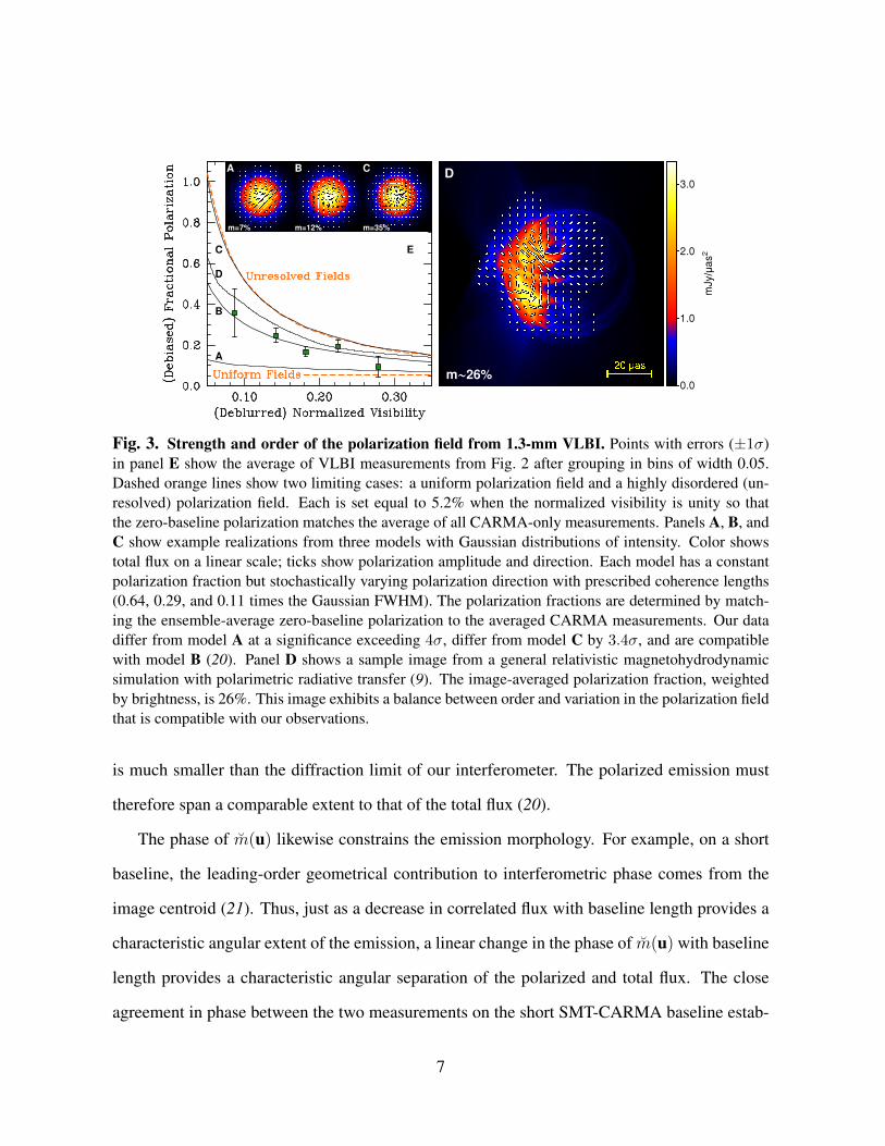
Fig. 3. Strength and order of the polarization field from 1.3-mm VLBI. Points with errors (±1σ)in panel E show the average of VLBI measurements from Fig. 2 after grouping in bins of width 0.05.Dashed orange lines show two limiting cases: a uniform polarization field and a highly disordered (un-resolved) polarization field. Each is set equal to 5.2% when the normalized visibility is unity so thatthe zero-baseline polarization matches the average of all CARMA-only measurements. Panels A, B, andC show example realizations from three models with Gaussian distributions of intensity. Color showstotal flux on a linear scale; ticks show polarization amplitude and direction. Each model has a constantpolarization fraction but stochastically varying polarization direction with prescribed coherence lengths(0.64, 0.29, and 0.11 times the Gaussian FWHM). The polarization fractions are determined by match-ing the ensemble-average zero-baseline polarization to the averaged CARMA measurements. Our datadiffer from model A at a significance exceeding 4σ, differ from model C by 3.4σ, and are compatiblewith model B (20). Panel D shows a sample image from a general relativistic magnetohydrodynamicsimulation with polarimetric radiative transfer (9). The image-averaged polarization fraction, weightedby brightness, is 26%. This image exhibits a balance between order and variation in the polarization fieldthat is compatible with our observations.

is much smaller than the diffraction limit of our interferometer. The polarized emission must

therefore span a comparable extent to that of the total flux (20).

The phase of m(u) likewise constrains the emission morphology. For example, on a short

baseline, the leading-order geometrical contribution to interferometric phase comes from the

image centroid (21). Thus, just as a decrease in correlated flux with baseline length provides a

characteristic angular extent of the emission, a linear change in the phase of m(u) with baseline

length provides a characteristic angular separation of the polarized and total flux. The close

agreement in phase between the two measurements on the short SMT-CARMA baseline estab-

7

lishes that the polarized and unpolarized flux are closely aligned, to within ∼10 µas when the

polarization angle of Sgr A∗ is relatively steady (Fig. S8). However, when variability is dom-

inant, we measure much larger offsets, up to ∼100 µas, implicating dynamical activity near

the black hole. For comparison, the apparent diameter of the innermost stable circular orbit is

6√

3/2RSch ≈ 73 µas, if the black hole of Sgr A∗ is not spinning. The tight spatial associ-

ation of this linear polarization with the 1.3-mm emission region then cements low-accretion

models for Sgr A∗ (11) which, combined with the measured spectrum in the submillimeter

bump and in the near-infrared, imply a magnetic field of tens of Gauss throughout the emitting

plasma (3, 4, 7).

Even amid magnetically driven instabilities and a turbulent accretion environment, several

effects can produce ordered fields near the event horizon. For example, as the orbits of the

accreting material around the black hole become circular, magnetic fields will be azimuthally

sheared by the differential rotation, resulting in a predominantly toroidal configuration (23). The

high image-averaged polarization associated with the emission region necessitates that such a

flow be viewed at high inclination since circular symmetry would cancel the polarization of a

disk viewed face-on. The striking difference between the stability of compact structures in the

total flux (17) relative to the rapid changes in the polarized structures on similar scales is then

most naturally explained via dynamical magnetic field activity through coupled actions of disk

rotation and turbulence driven by the magnetorotational instability (MRI) (24).

Alternatively, accumulation of sufficient magnetic flux near the event horizon may have led

to a stable, magnetically dominated inner region, suppressing the disk rotation and the MRI

(25–27). Emission from a magnetically dominant region provides an attractive explanation

for the long-term stability of the circular polarization handedness and the linear polarization

direction of Sgr A∗ (28, 29), and it has recently received observational support in describing

the cores of active galaxies with prominent jets (30–32). However, the close alignment of the

8

polarized and total emission (20) severely constrains multi-component emission models for the

quiescent flux, such as a bipolar jet (33) or a coupled jet-disk system (34). If a jet is present, then

this constraint suggests substantial differences between the emitting electron populations in the

jet and the accretion flow to ensure the dominance of a single component at 1.3 mm (27, 35).

With the advent of polarimetric VLBI at 1.3-mm wavelength, we are now resolving the

magnetized core of our Galaxy’s central engine. Our measurements provide direct evidence

of ordered magnetic fields in the immediate vicinity of Sgr A∗, firmly grounding decades of

theoretical work. Despite the extreme compactness of the emission region, we unambiguously

localize the linear polarization to the same region and identify spatial variations in the polariza-

tion direction. We also detect intra-hour variability and spatially resolve its associated offsets.

In the next few years, expansion of the EHT will enable imaging of these magnetic structures

and variability studies on the 20-second gravitational timescale (GM/c3) of Sgr A∗.

References and Notes

1. G. C. Bower, et al. Radio and Millimeter Monitoring of Sgr A*: Spectrum, Variability,

and Constraints on the G2 Encounter. Astrophys. J. 802, 69 (2015). doi:10.1088/0004-

637X/802/1/69.

2. F. Ozel, D. Psaltis, R. Narayan. Hybrid Thermal-Nonthermal Synchrotron Emission from

Hot Accretion Flows. Astrophys. J. 541, 234 (2000). doi:10.1086/309396.

3. J. Dexter, E. Agol, P. C. Fragile, J. C. McKinney. The Submillimeter Bump in Sgr A*

from Relativistic MHD Simulations. Astrophys. J. 717, 1092 (2010). doi:10.1088/0004-

637X/717/2/1092.

4. F. Yuan, R. Narayan. Hot Accretion Flows Around Black Holes. Annu. Rev. Astron. Astro-

phys. 52, 529 (2014). doi:10.1146/annurev-astro-082812-141003.

9

5. T. W. Jones, P. E. Hardee. Maxwellian synchrotron sources. Astrophys. J. 228, 268 (1979).

doi:10.1086/156843.

6. B. C. Bromley, F. Melia, S. Liu. Polarimetric Imaging of the Massive Black Hole at the

Galactic Center. Astrophys. J. 555, L83 (2001). doi:10.1086/322862.

7. F. Yuan, E. Quataert, R. Narayan. Nonthermal Electrons in Radiatively Inefficient Accre-

tion Flow Models of Sagittarius A*. Astrophys. J. 598, 301 (2003). doi:10.1086/378716.

8. A. E. Broderick, A. Loeb. Imaging optically-thin hotspots near the black hole horizon of

Sgr A* at radio and near-infrared wavelengths. Mon. Not. R. Astron. Soc. 367, 905 (2006).

doi:10.1111/j.1365-2966.2006.10152.x.

9. R. V. Shcherbakov, J. C. McKinney. Submillimeter Quasi-periodic Oscillations in Mag-

netically Choked Accretion Flow Models of SgrA*. Astrophys. J. 774, L22 (2013).

doi:10.1088/2041-8205/774/2/L22.

10. G. C. Bower, H. Falcke, M. C. Wright, D. C. Backer. Variable Linear Polarization from

Sagittarius A*: Evidence of a Hot Turbulent Accretion Flow. Astrophys. J. 618, L29 (2005).

doi:10.1086/427498.

11. D. P. Marrone, J. M. Moran, J.-H. Zhao, R. Rao. An Unambiguous Detection of Faraday

Rotation in Sagittarius A*. Astrophys. J. 654, L57 (2007). doi:10.1086/510850.

12. S. G. Jorstad, et al. Polarimetric Observations of 15 Active Galactic Nuclei at High Fre-

quencies: Jet Kinematics from Bimonthly Monitoring with the Very Long Baseline Array.

Astron. J. 130, 1418 (2005). doi:10.1086/444593.

13. G. C. Bower, M. C. H. Wright, D. C. Backer, H. Falcke. The Linear Polarization of Sagit-

tarius A*. II. VLA and BIMA Polarimetry at 22, 43, and 86 GHz. Astrophys. J. 527, 851

(1999). doi:10.1086/308128.

10

14. A. Eckart, et al. Polarimetry of near-infrared flares from Sagittarius A*. Astron. Astrophys.

455, 1 (2006). doi:10.1051/0004-6361:20064948.

15. M. Zamaninasab, et al. Near infrared flares of Sagittarius A*. Importance of near infrared

polarimetry. Astron. Astrophys. 510, A3 (2010). doi:10.1051/0004-6361/200912473.

16. S. S. Doeleman, et al. Event-horizon-scale structure in the supermassive black hole candi-

date at the Galactic Centre. Nature 455, 78 (2008). doi:10.1038/nature07245.

17. V. L. Fish, et al. 1.3 mm Wavelength VLBI of Sagittarius A*: Detection of Time-variable

Emission on Event Horizon Scales. Astrophys. J. 727, L36 (2011). doi:10.1088/2041-

8205/727/2/L36.

18. A. M. Ghez, et al. Measuring Distance and Properties of the Milky Way’s Cen-

tral Supermassive Black Hole with Stellar Orbits. Astrophys. J. 689, 1044 (2008).

doi:10.1086/592738.

19. S. Gillessen, et al. Monitoring Stellar Orbits Around the Massive Black Hole in the Galactic

Center. Astrophys. J. 692, 1075 (2009). doi:10.1088/0004-637X/692/2/1075.

20. Supplementary materials are available on Science Online.

21. M. D. Johnson, et al. Relative Astrometry of Compact Flaring Structures in Sgr A*

with Polarimetric Very Long Baseline Interferometry. Astrophys. J. 794, 150 (2014).

doi:10.1088/0004-637X/794/2/150.

22. V. L. Fish, et al. Imaging an Event Horizon: Mitigation of Scattering toward Sagittarius

A*. Astrophys. J. 795, 134 (2014). doi:10.1088/0004-637X/795/2/134.

11

23. S. Hirose, J. H. Krolik, J.-P. De Villiers, J. F. Hawley. Magnetically Driven Accretion

Flows in the Kerr Metric. II. Structure of the Magnetic Field. Astrophys. J. 606, 1083

(2004). doi:10.1086/383184.

24. S. A. Balbus, J. F. Hawley. A powerful local shear instability in weakly magnetized

disks. I - Linear analysis. II - Nonlinear evolution. Astrophys. J. 376, 214 (1991).

doi:10.1086/170270.

25. R. Narayan, I. V. Igumenshchev, M. A. Abramowicz. Magnetically Arrested Disk:

an Energetically Efficient Accretion Flow. Publ. Astron. Soc. Jpn. 55, L69 (2003).

doi:10.1093/pasj/55.6.L69.

26. J. C. McKinney, A. Tchekhovskoy, R. D. Blandford. General relativistic magneto-

hydrodynamic simulations of magnetically choked accretion flows around black holes.

Mon. Not. R. Astron. Soc. 423, 3083 (2012). doi:10.1111/j.1365-2966.2012.21074.x.

27. C.-K. Chan, D. Psaltis, F. Ozel, R. Narayan, A. Sadowski. The Power of Imaging: Con-

straining the Plasma Properties of GRMHD Simulations using EHT Observations of Sgr

A*. Astrophys. J. 799, 1 (2015). doi:10.1088/0004-637X/799/1/1.

28. G. C. Bower, H. Falcke, R. J. Sault, D. C. Backer. The Spectrum and Variability of Cir-

cular Polarization in Sagittarius A* from 1.4 to 15 GHz. Astrophys. J. 571, 843 (2002).

doi:10.1086/340064.

29. D. J. Munoz, D. P. Marrone, J. M. Moran, R. Rao. The Circular Polarization of Sagittar-

ius A* at Submillimeter Wavelengths. Astrophys. J. 745, 115 (2012). doi:10.1088/0004-

637X/745/2/115.

12

30. M. Zamaninasab, E. Clausen-Brown, T. Savolainen, A. Tchekhovskoy. Dynamically im-

portant magnetic fields near accreting supermassive black holes. Nature 510, 126 (2014).

doi:10.1038/nature13399.

31. P. Mocz, X. Guo. Interpreting MAD within multiple accretion regimes. Mon. Not. R. As-

tron. Soc. 447, 1498 (2015). doi:10.1093/mnras/stu2555.

32. I. Martı-Vidal, S. Muller, W. Vlemmings, C. Horellou, S. Aalto. A strong mag-

netic field in the jet base of a supermassive black hole. Science 348, 311 (2015).

doi:10.1126/science.aaa1784.

33. S. Markoff, G. C. Bower, H. Falcke. How to hide large-scale outflows: size constraints

on the jets of Sgr A*. Mon. Not. R. Astron. Soc. 379, 1519 (2007). doi:10.1111/j.1365-

2966.2007.12071.x.

34. F. Yuan, S. Markoff, H. Falcke. A Jet-ADAF model for Sgr A∗. Astron. Astrophys. 383,

854 (2002). doi:10.1051/0004-6361:20011709.

35. M. Moscibrodzka, H. Falcke. Coupled jet-disk model for Sagittarius A*: explaining the

flat-spectrum radio core with GRMHD simulations of jets. Astron. Astrophys. 559, L3

(2013). doi:10.1051/0004-6361/201322692.

Acknowledgments

EHT research is funded by multiple grants from NSF, by NASA, and by the Gordon and Betty

Moore Foundation through a grant to S.D. The Submillimeter Array is a joint project between

the Smithsonian Astrophysical Observatory and the Academia Sinica Institute of Astronomy

and Astrophysics. The Arizona Radio Observatory is partially supported through the NSF Uni-

versity Radio Observatories program. The James Clerk Maxwell Telescope was operated by

the Joint Astronomy Centre on behalf of the Science and Technology Facilities Council of the

13

UK, the Netherlands Organisation for Scientific Research, and the National Research Coun-

cil of Canada. Funding for CARMA development and operations was supported by NSF and

the CARMA partner universities. We thank Xilinx for equipment donations. A.B. receives fi-

nancial support from the Perimeter Institute for Theoretical Physics and the Natural Sciences

and Engineering Research Council of Canada through a Discovery Grant. Research at Perime-

ter Institute is supported by the Government of Canada through Industry Canada and by the

Province of Ontario through the Ministry of Research and Innovation. J.D. receives support

from a Sofja Kovalevskaja award from the Alexander von Humboldt Foundation. M.H. was

supported by a Japan Society for the Promotion of Science Grant-in-aid. R.T. receives support

from Netherlands Organisation for Scientific Research. Data used in this paper are available in

the supplementary materials.

Supplementary Materials

www.sciencemag.org

Supplementary Text

Figs. S1 to S8

Tables S1-S3

References (36-61)

Data S1 and S2

14

Supplementary Materials forResolved magnetic-field structure and variability

near the event horizon of Sagittarius A*Michael D. Johnson*, Vincent L. Fish, Sheperd S. Doeleman, Daniel P. Marrone, Richard

L. Plambeck, John F. C. Wardle, Kazunori Akiyama, Keiichi Asada, Christopher Beaudoin,Lindy Blackburn, Ray Blundell, Geoffrey C. Bower, Christiaan Brinkerink, Avery

E. Broderick, Roger Cappallo, Andrew A. Chael, Geoffrey B. Crew, Jason Dexter, MattDexter, Robert Freund, Per Friberg, Roman Gold, Mark A. Gurwell, Paul T. P. Ho, MarekiHonma, Makoto Inoue, Michael Kosowsky, Thomas P. Krichbaum, James Lamb, Abraham

Loeb, Ru-Sen Lu, David MacMahon, Jonathan C. McKinney, James M. Moran, RameshNarayan, Rurik A. Primiani, Dimitrios Psaltis, Alan E. E. Rogers, Katherine Rosenfeld, Jason

SooHoo, Remo P. J. Tilanus, Michael Titus, Laura Vertatschitsch, Jonathan Weintroub,Melvyn Wright, Ken H. Young, J. Anton Zensus, and Lucy M. Ziurys

*To whom correspondence should be addressed; E-mail: mjohnson@cfa.harvard.edu.

This PDF file includes:

Supplementary Text

Figs. S1 to S8

Tables S1-S3

References (36-61)

Other Supplementary Material for this manuscript includes the following:

Data S1 and S2

1

Supplementary Text

Site Details

Polarimetric calibration can be achieved in a general framework, but it depends on specific

details about each of the involved stations. For example, we must account for the field rotation

angle – the relative orientation of the feed with respect to a fixed direction on the sky – which

varies with time. The following list provides the specific details needed for each of our sites:

• CARMA Phased Array: The CARMA phased array combined antennas C2, C3, C4,

C5, C6, C8, C9, and C14. After the second day, the refrigerator dewar in antenna C3

failed; antenna C3 was then replaced by C13 in the phased sum. Sites with an index up to

6 are 10.4-m antennas; the remainder are 6.1-m antennas. Each telescope recorded both

circular polarizations. The phasing efficiency was typically over 90%, even for weak

sources. For each CARMA antenna, the field rotation angle is simply the parallactic

angle. As for all sites except the CARMA reference antenna, the CARMA phased array

recorded two 512 MHz bands (each with 480 MHz of usable bandwidth). We refer to

these as the “high” (centered on 229.601 GHz) and the “low” (centered on 229.089 GHz)

bands.

• CARMA Reference Station: CARMA antenna C1 was used separately to record both

circular polarizations in the low band only.

• SMT: The SMT recorded both circular polarizations. The two polarizations have separate

Gunn oscillators, resulting in a stochastic phase drift (up to ∼10◦/hour) between them.

For the SMT, the field rotation angle is the sum of the parallactic and elevation angles.

• Phased SMA: The phased SMA combined seven of the eight SMA antennas and recorded

only one circular polarization at a time. However, because the quarter-wave plates (QWPs)

2

on each antenna can be rapidly rotated, we alternated the recorded polarization: LCP on

long scans (4-8 minutes) with interleaved RCP on short scans (30 seconds). The esti-

mated phasing efficiency differed between the high and low bands, with medians of 83%

and 65%, respectively. For the SMA, the field rotation angle is 45◦ minus the elevation

angle plus the parallactic angle.

• JCMT: The JCMT recorded a single polarization (RCP), and its field rotation angle is

the parallactic angle.

Correlation Procedure

We correlated our data using the Haystack Mark4 correlator (36). For subsequent fringe-fitting,

we used the Haystack Observatory Post-processing System. Because a typical atmospheric

coherence time (∼5 seconds) is much shorter than our scan lengths (∼5 minutes), we performed

fringe-fitting in three steps (37, 38):

1. First, a blind fringe search determined the fringe-rate and the fringe-delay, as well as the

RCP-LCP delay differences for dual-polarization stations, which were nearly constant

each day. Concurrently, this pass estimated the time-dependent phase, the “ad hoc” phase,

on parallel-hand baselines to the CARMA phased array for one chosen polarization. This

phase included contributions from the source, the atmosphere, the instrument, and thermal

noise; the most rapid changes were from the atmosphere and noise. To preserve the

polarimetric identities (described below), there was necessarily a single ad hoc phase for

both polarizations. Hence, for the ad hoc phases, the JCMT and the SMA were considered

to be a single station.

2. A second pass removed the ad hoc phases calculated in the first pass before fringe fitting.

When possible, the removed ad hoc phases were determined from the opposite band (low

3

or high) to avoid biasing weak parallel-hand detections by removing the phases associated

with their own thermal noise.

3. A third and final pass used the delay and rate solutions from the second pass together with

the RCP-LCP delay offsets and ad hoc phases from the first pass to coherently average

parallel- and cross-hand visibilities over scans.

Polarimetric Calibration Procedure

Definitions and Conventions. Polarimetric VLBI enables studies of the images of the Stokes

parameters Q, U , and V in addition to that of total intensity, I. Polarimetric interferometry on

a baseline u (length in wavelengths) is sensitive to the respective Fourier components of these

images; e.g., Q(u) (37, 39). Moreover, as we have mentioned in the main text and discuss in

more depth subsequently, fractional polarization in the visibility domain provides an especially

robust observable: m(u) ≡[Q(u) + iU(u)

]/I(u). Note that we use a breve rather than a

tilde to emphasize that this interferometric fractional polarization holds no Fourier relationship

with its image-domain analog, m(x) ≡ [Q(x) + iU(x)] /I(x). Also, fractional polarization in

the Fourier domain is not constrained to have amplitude less than unity, and m(u) includes

contributions to phase from the geometrical distribution of polarized and total flux (e.g., in the

phase of I(u)). The linear polarization, Q + iU , is commonly written in the form I|m|e2iχ,

where 0 ≤ |m| ≤ 1 is the polarization fraction and χ is the polarization direction (or angle).

We use the same terminology to refer to the analogous quantities for m, although (as we have

noted) these must be interpreted with care.

Imperfections in the instrumental response distort the relationship between the measured

polarization and the source polarization. These imperfections can be conveniently described

by a Jones matrix, J; estimates of the Jones matrix can then be used to correct the distortion.

The Jones matrix is commonly decomposed into “gain” and “leakage” terms, GR,L and DR,L,

4

respectively. Specifically, after accounting for field rotation by an angle φ relative to a fixed

(celestial) basis, the measured fields E ′R,L can be written(E ′RE ′L

)≈(GR 00 GL

)(1 DR

DL 1

)(e−iφ 0

0 eiφ

)(ER

EL

)≡ J

(ERe

−iφ

ELeiφ

). (S1)

When transformed from a circular-polarization basis to a linear-polarization basis, φ is simply

the angle in a 2× 2 rotation matrix.

Linearizing in the source polarization and leakage terms and neglecting circular polarization

yields the following approximations (37):

〈L1R∗2〉

〈L1L∗2〉≈(G2,R

G2,L

)∗ [m∗(−u12)e2iφ2 +D1,Le

−2i(φ1−φ2) +D∗2,R]

(S2)

〈L1R∗2〉

〈R1R∗2〉≈(G1,L

G1,R

)[m∗(−u12)e2iφ1 +D1,L +D∗2,Re

2i(φ1−φ2)]

〈R1L∗2〉

〈L1L∗2〉≈(G1,R

G1,L

)[m(u12)e−2iφ1 +D1,R +D∗2,Le

−2i(φ1−φ2)]

〈R1L∗2〉

〈R1R∗2〉≈(G2,L

G2,R

)∗ [m(u12)e−2iφ2 +D1,Re

2i(φ1−φ2) +D∗2,L]

〈R1R∗2〉

〈L1L∗2〉≈(G1,R

G1,L

)(G2,R

G2,L

)∗e−2i(φ1−φ2).

Here, m(u12) represents the fractional polarization in the visibility domain on a baseline joining

sites 1 and 2, φi is the field rotation angle at site i, and we have introduced the simplified

notation Ri ≡ E ′R,i. Note that to recover the full information m(±u) on a given baseline, both

polarizations must be recorded at each site.

These equations demonstrate the utility of fractional polarization in VLBI. Namely, varia-

tions in the complex gains only affect these quotients through their changes relative to the gain

of the opposite circular polarization at the same site. Also, the leakage terms introduce spuri-

ous linear polarizations, which differ from the source polarization terms in their dependence on

field rotation. Hence, polarimetric calibration relies heavily upon long calibration tracks with

wide sampling of the field rotation. Fig. S1 shows the field rotation angles for our two primary

calibration targets and for Sgr A∗.

5

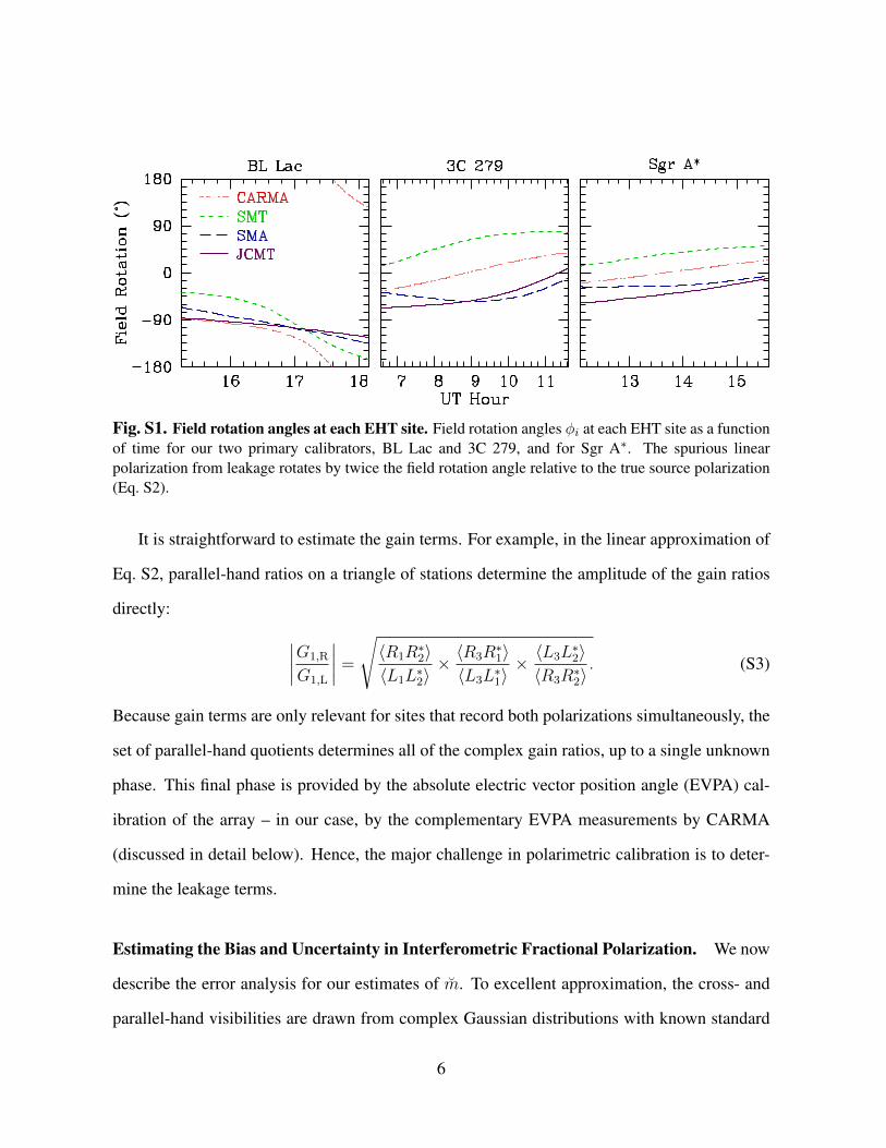
Fig. S1. Field rotation angles at each EHT site. Field rotation angles φi at each EHT site as a functionof time for our two primary calibrators, BL Lac and 3C 279, and for Sgr A∗. The spurious linearpolarization from leakage rotates by twice the field rotation angle relative to the true source polarization(Eq. S2).

It is straightforward to estimate the gain terms. For example, in the linear approximation of

Eq. S2, parallel-hand ratios on a triangle of stations determine the amplitude of the gain ratios

directly: ∣∣∣∣G1,R

G1,L

∣∣∣∣ =

√〈R1R∗2〉〈L1L∗2〉

× 〈R3R∗1〉〈L3L∗1〉

× 〈L3L∗2〉〈R3R∗2〉

. (S3)

Because gain terms are only relevant for sites that record both polarizations simultaneously, the

set of parallel-hand quotients determines all of the complex gain ratios, up to a single unknown

phase. This final phase is provided by the absolute electric vector position angle (EVPA) cal-

ibration of the array – in our case, by the complementary EVPA measurements by CARMA

(discussed in detail below). Hence, the major challenge in polarimetric calibration is to deter-

mine the leakage terms.

Estimating the Bias and Uncertainty in Interferometric Fractional Polarization. We now

describe the error analysis for our estimates of m. To excellent approximation, the cross- and

parallel-hand visibilities are drawn from complex Gaussian distributions with known standard

6

deviations. A measured fractional polarization, denoted with a prime (′), can then be related to

the true fractional polarization as

m′ = m

(1 + εP/SP

1 + εI/SI

), (S4)

where SP is the signal-to-noise ratio of the measured P , SI is the signal-to-noise ratio of the

measured I, and the ε are complex Gaussian random variables with a standard deviation of

unity in their real and imaginary parts.

Because we rely on strong parallel-hand detections for fringes, SI � 1 for all of our mea-

surements. Thus,

m′ ≈ m (1 + εP/SP) (1− εI/SI) . (S5)

In addition, nearly all of our measurements have SP >∼ 1, so m′ is approximately a complex

Gaussian random variable centered on m with a signal-to-noise of Sm ≈ 1/√

1/S2I + 1/S2

P.

[This approximation is best for our measurements with the highest fractional polarizations be-

cause they have SP � 1.] A gain correction will scale m′, keeping the signal-to-noise ratio Sm

constant, while a leakage correction will shift m′, keeping the root-mean-square noise |m′|/Sm

constant but changing the signal-to-noise ratio (see Eq. S2).

Because of thermal noise, estimates A′ = |m′| of the fractional polarization amplitude

|m| will be biased upward. To derive an unbiased estimator A of |m|, note that A will have

a standard deviation of σA ≈ A/Sm (39). As a result, 〈A2〉 = |m|2 + σ2A. Since 〈A′2〉 =

|m|2 + 2σ2A, an appropriate unbiased estimator of |m| is A =

√A′2 − σ2

A (imaginary values

are set equal to zero). This standard result for polarimetry was rigorously derived in (40) via a

maximum-likelihood approach.

Interestingly, this estimator differs from the estimator for incoherent averaging ofM visibil-

ities: Ainc =√〈A′2i 〉M − 2σ2

A (41), where 〈. . . 〉M denotes an average of M samples {A′i}. The

reason for the difference is that the derivation of Ainc implicitly assumes M → ∞ so that Ainc

7

has no associated noise. For a finite number of samples, each having noise σA <∼ A, the ampli-

tude estimator will instead have a standard deviation of σA/√M . In this case, an unbiased esti-

mator that is appropriate for an arbitrary number of samples is A =√〈A′2i 〉M − σ2

A(2− 1/M).

Taking M = 1 and M → ∞ then recovers the standard results for polarization and incoherent

averaging, respectively.

Although these results assume high signal-to-noise for both I and P , they are excellent for

our data. For instance, with SI = 8 and SP = 3, the above prescription to estimate |m| has

a fractional bias less than 1% and correctly estimates the signal-to-noise ratio to within 10%.

Even when SI = 6.5 (the cutoff we have used) and SP = 2, the fractional bias is less than 2%

and the noise is estimated correctly to within 12%. Furthermore, while the quotient of Gaussian

random variables is not Gaussian and results in a high tail at large fractional polarizations, the

consistency in our results between different frequency bands demonstrates that our measured

high polarization fractions are not statistical outliers.

Data Subset and Preprocessing for Polarimetric Calibration. We performed minimal pro-

cessing on the visibilities before deriving our calibration solution. Specifically, we only in-

cluded fractional polarizations for which the parallel-hand visibility had a signal-to-noise ratio

(SNR) exceeding 8. We then used the parallel-hand ratios to estimate the RCP-LCP phase drift

at the SMT by assuming that the RCP-LCP phase at CARMA was constant on each day. We

performed a weighted (by SNR) average of the five nearest phase estimates for each time to

invert the phase drift. For calibration, we did not include short (30 second) scans on any base-

line except those to the SMA (RCP). We derived our calibration solutions using only 3C 273,

3C 279, and BL Lac. These sources were all bright and exceptionally compact.

For the purposes of calibration, we also included data on the∼200-m JCMT-SMA baseline.

Although information on this baseline was redundant with that of CARMA, polarization mea-

surements on the JCMT-SMA baseline provided excellent information about the leakages at

8

these two stations, especially because their field rotation angles differed by the source elevation

angle minus 45◦. However, because the JCMT and the SMA each recorded a single polarization,

we could not compute the instantaneous fractional polarization on this short baseline. Never-

theless, we estimated fractional polarization using non-simultaneous estimates of the cross- and

parallel-hand visibilities. The parallel-hand products were estimated using the short (30 sec-

ond) scans when the SMA recorded RCP, and the cross-hand products were estimated using the

immediately following long (∼5 minute) scans. Although the phase accuracy of these fractional

polarizations is unreliable, the amplitude is robust and varies as the field rotation angles changes

at each site because of the changing contribution of the leakage terms.

Complementary Measurements with CARMA. Normal observations with CARMA were

made in parallel with the VLBI observations, and these data were used to measure the po-

larizations of all sources. In full polarization mode, the CARMA correlator provides 4 GHz

bandwidth (4 bands × 500 MHz × 2 sidebands) for each of the 4 polarization products (RR,

LL, RL, LR) on each of the 105 baselines that connect the 15 10.4-m and 6.1-m telescopes.

The CARMA receivers operate in double sideband mode, so that signals both above and

below the local oscillator frequency are downconverted to the intermediate frequency. A 90◦

phase-switching pattern applied to the local oscillators allows these signals to be separated at

the correlator. This phase switching pattern is removed by the VLBI beamformer that sums

together signals from the 8 antennas that are phased together; thus, normal observations are

possible with these telescopes during VLBI scans. However, phase switching must be disabled

to the single CARMA reference antenna so that it may be treated as a completely independent

VLBI station; normal CARMA observations with this antenna are possible only between VLBI

scans.

Polarization observations require two additional calibrations beyond the usual gain, pass-

band, and flux calibrations. The first of these calibrations corrects for the delay difference

9

between the R and L channels. Because of the cabling in the correlator room, this delay dif-

ference varies from correlator band to correlator band as well as from antenna to antenna. To

calibrate the R-L delay, one must observe a linearly polarized source with a known position an-

gle. Linearly polarized noise sources in the telescope receiver cabins are used for this purpose at

CARMA. Each noise source consists simply of a wire grid that is rotated into the beam in front

of the receiver. With the grid in place, horizontally polarized radiation entering the receiver

originates from an ambient temperature absorber, while vertically polarized radiation originates

from the sky. Thus, there is a strong net horizontal polarization. The L-R phase difference is

measured on a channel-by-channel basis from LR autocorrelation spectra obtained with the grid

in place. Upper and lower sideband signals cannot be separated in autocorrelation spectra, but

it is reasonable to assume that the R-L delays are nearly identical for corresponding channels

in the upper and lower sidebands because the delays are caused almost entirely by cable length

differences, which affect these signals equally.

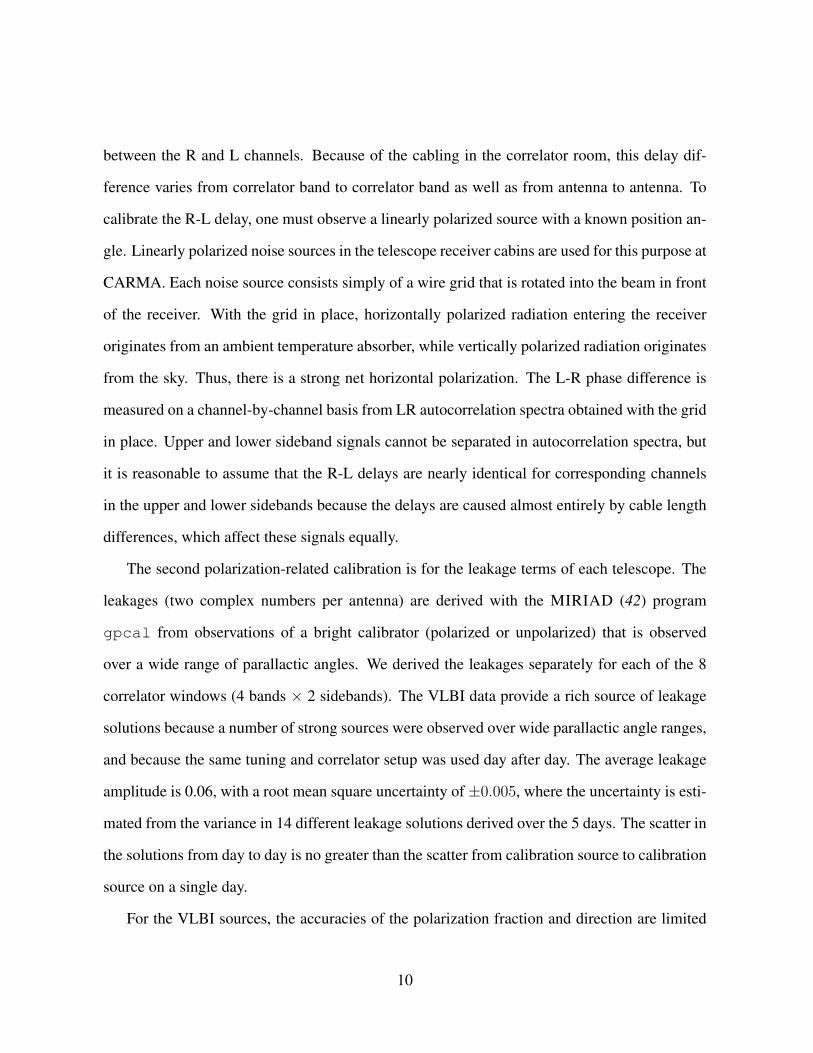
The second polarization-related calibration is for the leakage terms of each telescope. The

leakages (two complex numbers per antenna) are derived with the MIRIAD (42) program

gpcal from observations of a bright calibrator (polarized or unpolarized) that is observed

over a wide range of parallactic angles. We derived the leakages separately for each of the 8

correlator windows (4 bands × 2 sidebands). The VLBI data provide a rich source of leakage

solutions because a number of strong sources were observed over wide parallactic angle ranges,

and because the same tuning and correlator setup was used day after day. The average leakage

amplitude is 0.06, with a root mean square uncertainty of ±0.005, where the uncertainty is esti-

mated from the variance in 14 different leakage solutions derived over the 5 days. The scatter in

the solutions from day to day is no greater than the scatter from calibration source to calibration

source on a single day.

For the VLBI sources, the accuracies of the polarization fraction and direction are limited

10

by systematic errors in the leakage and R-L delay calibrations rather than by thermal noise;

hence, fractional polarizations were not corrected for noise bias. To estimate the effects of

uncertainties in the leakage calibrations, we applied the ensemble of leakage solutions to the

data and computed the variance in the resulting source polarizations and position angles. Errors

in the R-L delay calibration affect only the absolute EVPA of the sources. The uncertainty in the

EVPA is estimated to be±3◦, based on polarization measurements of Mars obtained at CARMA

in 2014 May (43). Near the limb of the planet, emission from Mars is radially polarized (44);

deviations from radial polarization were used to estimate the absolute EVPA uncertainty.

CARMA leakage corrections for VLBI calibration were derived separately for the 2 corre-

lator windows that were used for the “high” and “low” bands. For the phased set of 8 antennas,

the vector average of the leakages for these 8 telescopes was used.

Assumptions and Procedure for Deriving a Calibration Solution. To derive our complete

calibration solution for the VLBI array, we made several assumptions about the data. First, we

assumed that visibilities on nearly identical baselines (i.e., to the SMA/JCMT or to the phased

CARMA/reference CARMA) should match. We also assumed that the fractional polarization

seen on the Phased CARMA−Reference CARMA baseline was identical to the fractional polar-

ization determined by CARMA for each scan. We assumed that the station gain ratios GR/GL

were constant over each day (with the exception of the stochastic phase drift at the SMT), and

that the leakage terms at each site were constant throughout the observation (except for the

modified array membership in the CARMA phased array).

To account for the unknown source polarization structure in a general way, we introduced

a piecewise-linear approximation for the polarization dependence on baseline: on each base-

line, the source polarization was allowed to vary linearly between points (“knots”) separated by

a fixed amount of time (we used 1-hour spacings). We made no assumptions about the rela-

tionship between the source polarization on different baselines or the consistency of the source

11

polarization on different days.

After enforcing these assumptions, we performed a weighted least-squares fit to the low-

band data using the linearized approximation of Eq. S2. After this fit, we dropped all data

points with >4σ departure from the fitted model – usually a few percent of the data and almost

exclusively very-high-SNR (>∼100) quotients of parallel-hand visibilities. We then repeated the

least-squares fit, typically with negligible change from the first iteration.

The high-band data could not be independently calibrated in the same way because they lack

the CARMA reference antenna and because disk failures resulted in the loss of high-band data

for the RCP of the CARMA phased array on days 85 and 86. Instead, we derived a high-band

calibration solution by fitting the high-band data to the calibrated low-band data. As a result, the

two bands can be expected to have independent thermal noise but equivalent systematic errors

in the calibration solution.

Estimation of Calibration Uncertainties. The two major sources of uncertainty in our cal-

ibration solution are from thermal noise in the data and from the unknown source structure.

We refer to these as thermal uncertainty and systematic uncertainty, respectively. The thermal

uncertainty can be estimated by analyzing the χ2 hypersurface of the fitted calibration solu-

tion; the systematic uncertainty can be estimated by shifting the locations of the knots in the

piecewise-linear source polarization model.

To determine the cumulative uncertainty, we employed a Monte Carlo error analysis. First,

we successively shifted the piecewise-linear knots in increments of five minutes. Then, for each

shift, we generated ten data sets in which random thermal noise equal to that of the original

measurements was added to the measurements. For each such possibility, we independently

derived a calibration solution. We used the mean and standard deviation of the resulting set of

solutions to define our final calibration solution and uncertainty. Fig. S2 shows the results of

our calibration analysis including uncertainties estimated from this Monte Carlo analysis.

12

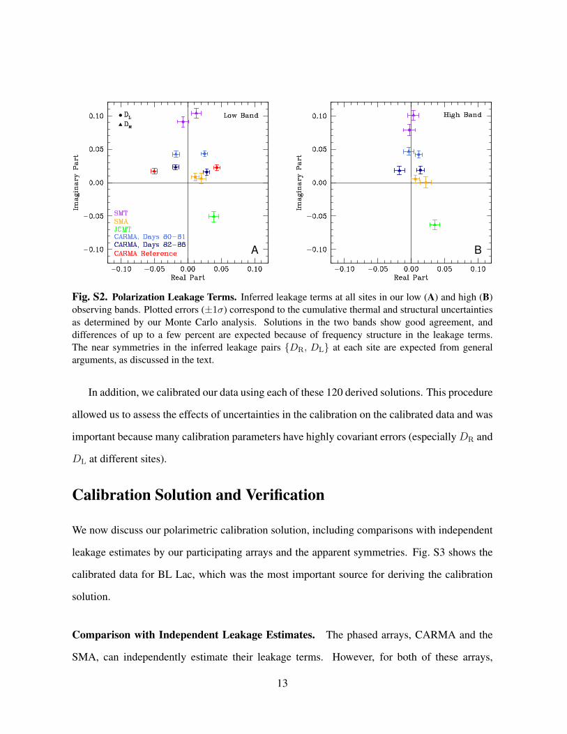
A B

Fig. S2. Polarization Leakage Terms. Inferred leakage terms at all sites in our low (A) and high (B)observing bands. Plotted errors (±1σ) correspond to the cumulative thermal and structural uncertaintiesas determined by our Monte Carlo analysis. Solutions in the two bands show good agreement, anddifferences of up to a few percent are expected because of frequency structure in the leakage terms.The near symmetries in the inferred leakage pairs {DR, DL} at each site are expected from generalarguments, as discussed in the text.

In addition, we calibrated our data using each of these 120 derived solutions. This procedure

allowed us to assess the effects of uncertainties in the calibration on the calibrated data and was

important because many calibration parameters have highly covariant errors (especiallyDR and

DL at different sites).

Calibration Solution and Verification

We now discuss our polarimetric calibration solution, including comparisons with independent

leakage estimates by our participating arrays and the apparent symmetries. Fig. S3 shows the

calibrated data for BL Lac, which was the most important source for deriving the calibration

solution.

Comparison with Independent Leakage Estimates. The phased arrays, CARMA and the

SMA, can independently estimate their leakage terms. However, for both of these arrays,

13

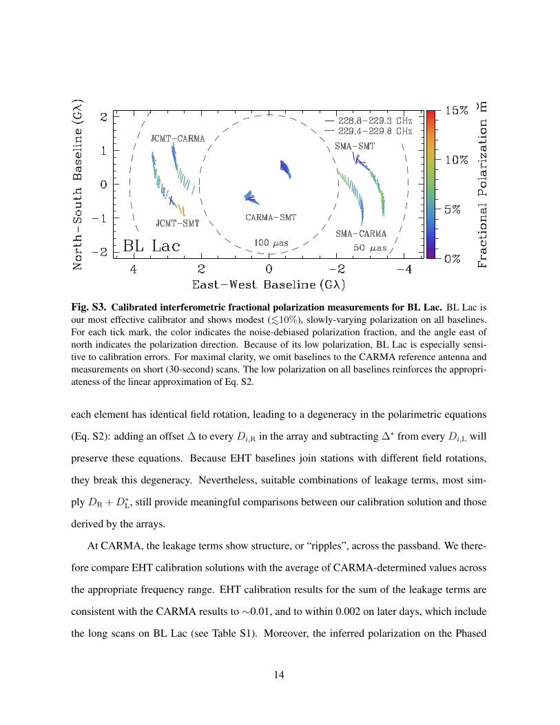
Fig. S3. Calibrated interferometric fractional polarization measurements for BL Lac. BL Lac isour most effective calibrator and shows modest (<∼10%), slowly-varying polarization on all baselines.For each tick mark, the color indicates the noise-debiased polarization fraction, and the angle east ofnorth indicates the polarization direction. Because of its low polarization, BL Lac is especially sensi-tive to calibration errors. For maximal clarity, we omit baselines to the CARMA reference antenna andmeasurements on short (30-second) scans. The low polarization on all baselines reinforces the appropri-ateness of the linear approximation of Eq. S2.

each element has identical field rotation, leading to a degeneracy in the polarimetric equations

(Eq. S2): adding an offset ∆ to every Di,R in the array and subtracting ∆∗ from every Di,L will

preserve these equations. Because EHT baselines join stations with different field rotations,

they break this degeneracy. Nevertheless, suitable combinations of leakage terms, most sim-

ply DR +D∗L, still provide meaningful comparisons between our calibration solution and those

derived by the arrays.

At CARMA, the leakage terms show structure, or “ripples”, across the passband. We there-

fore compare EHT calibration solutions with the average of CARMA-determined values across

the appropriate frequency range. EHT calibration results for the sum of the leakage terms are

consistent with the CARMA results to ∼0.01, and to within 0.002 on later days, which include

the long scans on BL Lac (see Table S1). Moreover, the inferred polarization on the Phased

14

Site CARMA DR +D∗L EHT DR +D∗L

CARMA Reference Antenna −0.009 + 0.000i −0.008− 0.006iCARMA Phased Array, Days 080-081 0.013 + 0.003i 0.001− 0.001iCARMA Phased Array, Days 082-086 0.010 + 0.006i 0.010 + 0.007i

Table S1. Comparisons of our low-band leakage solution for CARMA with independent esti-mates using only CARMA data.

CARMA-Reference CARMA baseline matches the values determined by CARMA, even for

sources (such as Sgr A∗) that were not included in the calibration.

At the SMA, the leakage terms have a small (∼2%) random component plus a linear slope

in their real part with frequency, consistent with the expected leakage incurred by departures

from the tuned frequency of the QWPs (45). The imaginary parts of the leakage terms may

reflect orientation errors in the QWPs. Best estimates using a combination of historical data

and other calibration measurements from 2013 give DL ≈ 0.015 − 0.009i − ∆∗ and DR ≈

0.018 + 0.005i+ ∆ for some unknown ∆; however, the imaginary parts of these measurements

are uncertain to ∼1% because of slight orientation shifts of the QWPs upon successive re-

installations. The average real part is then 0.017, which is quite close to the average of 0.015

from the EHT calibration solution. The difference in imaginary parts differs from the EHT

calibration solution by 2%, consistent with the effects of different QWP installations.

This independent analysis for CARMA and the SMA was done in MIRIAD (42), which

follows slightly different conventions than ours. To fix the complex degree of freedom in

connected-element calibration, MIRIAD imposes the constraint∑

iDi,R =∑

iD∗i,L. Also,

the field rotation angles used in MIRIAD differ by a constant offset δφ from our conven-

tions, rotating DR by 2δφ and DL by −2δφ (δφ is specified via the MIRIAD header parameter

evector). Lastly, MIRIAD employs an opposite baseline ordering convention to ours, intro-

ducing an overall conjugation of both DR and DL (46).

15

Symmetries in the Leakage Terms. Our derived calibration solution exhibits clear symme-

tries between the left and right leakage terms. Because such symmetries are not included as

prior constraints in our calibration procedure but are expected from general considerations,

they provide additional validation for the calibration solution.

For example, the inferred leakage terms at CARMA and the SMT have DR ≈ −D∗L. This

symmetry is expected whenever the Jones matrix acts in such a way that the power is preserved

and the outputs are orthogonal (i.e., if J is unitary: J−1 = J†) (see Appendix D of (37) or (47)).

Indeed, many instrumental effects produce a unitary Jones matrix. Common examples include

any rotation of orthogonal feeds or of a QWP, and departures from the tuned frequency of a

QWP.

For sites that do not have orthogonal feeds (i.e., the SMA and the JCMT), the situation is

slightly different. For instance, the general action of the QWP system at the SMA is described

in (45) and gives leakage terms that satisfy DR = D∗L (when an error in the QWP retardation

is included but not in the field transmission), regardless of the orientation of the feed or of the

QWP. As a specific example of this relationship, for errors that only arise from a frequency

offset from the tuned frequency of the QWP, the left and right leakage terms will be real and

equal. Note that this relationship differs from the previous result (DR = −D∗L) because of the

feed configuration rather than the feed (or QWP) orientation.

Possible Elevation Dependence of Leakage Terms. Our current calibration solution has no

allowance for elevation dependence of the leakage terms. Nevertheless, several features in the

calibrated data suggest that elevation-dependent leakage effects are small. Most directly, the

close agreement of the fractional polarization on the SMT-CARMA baseline with CARMA-

only measurements of Sgr A∗ (e.g., Fig. S4) shows that neither the SMT nor CARMA can have

large elevation dependence for their leakage terms. This result is especially secure because the

Sgr A∗ data was not used to derive the calibration solution. Elevation-dependent leakage at

16

the SMA and JCMT would appear in the comparison between redundant measurements to the

two stations (when the SMA sampled RCP) and also in non-simultaneous amplitude ratios on

the JCMT-SMA baseline (discussed above). These comparisons constrain elevation-dependent

leakage changes to be <∼0.01 for our current data at all sites – comparable to the derived uncer-

tainties of our leakage terms (Fig. S2) and of negligible importance for our current results.

Additional Calibration Considerations for Sgr A*. Although the low polarization of BL Lac

justifies the linear approximation for the polarimetric equations (Eq. S2) when deriving our cal-

ibration solution, the higher polarization fractions that we observe on long baselines to Sgr A∗

can introduce errors from higher-order terms. Nevertheless, higher order corrections to the in-

ferred m(u) are proportional to the products of m(u)2 and m(u)m(−u) with a leakage term,

and these corrections are within our current thermal noise.

Another consideration for the long-baseline measurements of Sgr A∗ is the effects of cir-

cular polarization. To leading order, circular polarization scales the parallel-hand visibilities

by (1± v), where v ≡ V/I is the fractional circular polarization in the visibility domain and

+/- corresponds to RCP/LCP. Although the fractional image-averaged circular polarization for

Sgr A∗ at λ=1.3 mm is only ≈1% (29), the fractional circular polarization v on long baselines

could be an order of magnitude higher, just as we observe for the fractional linear polarization

m.

We can robustly estimate v by comparing pairs of RCP and LCP parallel-hand visibilities

on baselines to the SMA, using adjacent long/short scans with the SMA sampling opposite po-

larization states. However, because the short scans have low-SNR, we have only five measure-

ments suitable for comparison. These measurements show no statistically significant detection

of circular polarization, with thermal noise giving 1σ uncertainties ranging from 11% to 20%

for individual estimates of v. Even within these crude limits, the allowed circular polarization is

insufficient to produce the distinctive asymmetry that we see in m(±u) on long baselines, often

17

in excess of a factor of three difference, which would require an implausibly large v >∼ 50%.

The circular polarization v can also be estimated using only long scans by comparing op-

posite parallel-hand visibilities on baselines to the SMA (LCP) with those to the JCMT (RCP).

However, this comparison is dominated by relative uncertainties in the time-variable gains at

these sites (which do not affect m).

Amplitude Calibration Procedure and Results.

Our amplitude calibration (i.e., the estimation of |I(u)|) followed a similar methodology to

previous work with the EHT (17, 48, 49) and will be presented in detail elsewhere. We now

briefly summarize the calibration procedure and results.

Amplitude Calibration Strategy. After correlation, we estimated parallel-hand visibility am-

plitudes via incoherent averaging (41). Incoherent averaging begins by coherently averaging

visibilities over a specified segmentation time and then incoherently averages the resulting set

of visibilities. To avoid a loss of signal, the segmentation time must be shorter than the timescale

of differential phase fluctuations between sites; in our case, the dominant fluctuations are from

the atmosphere, with a typical timescale of 5-10 seconds. In addition, while incoherent averag-

ing provides a nearly optimal estimator of the signal amplitude when the SNR of each averaged

segment is high, it is severely sub-optimal when the segment SNR is low. Because of these two

considerations, we first performed incoherent averaging with a 1-second segmentation time;

for scans with a resulting SNR less than 15, we then repeated the incoherent averaging with a

segmentation time of 6 seconds.

We next converted the estimated visibilities to physical units of correlated flux density by

applying an a priori calibration solution. This solution required estimates of the antenna gain

(Jy/K), system temperature, and atmospheric opacity for each station and each scan. For the

18

participating phased arrays (CARMA and the SMA), we also included scan-by-scan estimates

of the phasing efficiency. Because our present analysis is focused on the normalized visibility –

i.e., the correlated flux density on a given baseline divided by the simultaneous correlated flux

density on a zero-baseline – the conversion to physical units does not affect our results but time

variability of the gains does.

To solve for the remaining time-variable gains at each station and in each circular polariza-

tion, we assumed that the gains have a constant ratio |GR|/|GL| per station per day – an iden-

tical assumption to our polarization calibration and an assumption that was validated by com-

paring the RCP and LCP parallel-hand correlations between dual-polarization stations. Next,

we merged consecutive short/long scans. Doing so provides an effective parallel-hand, zero-

baseline interferometer on Hawaii (SMA-JCMT) during the short scans that can be used to

estimate the gains for the adjacent long scans. For each merged scan, we then solved for a

calibration solution using a least-squares minimization of all measurements. For these solu-

tions, we assumed that the circular polarization is zero, although our resultant solution would

not eliminate the imprint of circular polarization because we do not solve for separate RCP and

LCP gains.

The resulting gain solution is quite robust, a consequence of the particular baseline redun-

dancy of the EHT. To understand the reason for this robustness, consider two pairs of co-located

stations: {A,A′} and {B,B′}. [By co-located, we simply mean that the visibility VAA′ is equal

to what would be measured by a zero-baseline interferometer.] These provide two independent

closure amplitudes:

A1 =

∣∣∣∣VABVA′B′

VAB′VA′B

∣∣∣∣ (S6)

A2 =

∣∣∣∣VABVA′B′

VAA′VBB′

∣∣∣∣ ,where VAB denotes a visibility on the baseline joining stations A and B. Closure amplitudes

19

Fig. S4. Comparison of CARMA-only and SMT-CARMA fractional polarization measurementsfor Sgr A∗. Comparison of the calibrated fractional polarization measurements made by CARMA withthose measured on the SMT-CARMA baseline for Sgr A∗ on one day. For the SMT-CARMA base-line, we averaged the pair of measurements m(±u) to eliminate the linear dependence of m on base-line (see Eq. S9). Errors (1σ) denote the aggregate of thermal and systematic uncertainties; system-atic uncertainties (0.5%) are dominant for measurements by CARMA but are subdominant for thoseof the SMT-CARMA baseline. Fitting all measurements for a single relative factor f in the polariza-tions (f ≡ mCARMA/mSMT−CARMA) gives f = 0.97 ± 0.03 on this day, with a reduced chi-squaredχ2

red ≈ 0.79 (χ2red < 1 may suggest that systematic errors for CARMA are overestimated). This close

agreement, f ≈ 1, rules out the possibility of substantial unpolarized or differentially polarized emission(relative to the compact emission) on scales between a few hundred µas and ∼10′′. Such emission couldnot contribute more than ∼10% of the total flux in these observations.

such as these are especially valuable because they are immune to station-based gain fluctua-

tions (39). The first of these is a “trivial” closure amplitude: A1 = 1. However, the second,

A2 = |VAB/VAA′ |2, gives the squared normalized visibility on the A–B baseline. As a result,

the normalized visibility on any baseline joining two pairs of co-located sites is a closure quan-

tity. The limiting noise on such baselines will likely be thermal noise rather than systematic

uncertainties. For our current data, the phased CARMA/reference CARMA and SMA/JCMT

pairs provide this degree of redundancy, so we can estimate the CARMA-SMA/JCMT normal-

ized visibility as a closure quantity.

However, no visibility on a baseline to the SMT can be considered known or can be com-

pared to other identical measurements. As a result, the gain calibration of the SMT cannot be

20

improved beyond the a priori calibration solution without additional assumptions about source

structure. Nevertheless, our polarization measurements suggest one robust pathway to deter-

mine an approximate gain solution at the SMT (to within ∼10-20%). Specifically, our po-

larization measurements argue that Sgr A∗ is so compact that we can approximate the SMT-

CARMA baseline as yet another zero-baseline (i.e., a baseline that does not resolve the image)

(see Fig. S4). Because the visibility amplitude |I(u)| is always maximum when u = 0, this

strategy determines a strict upper limit for visibility amplitudes on baselines to the SMT. Thus,

to conservatively bracket the remaining uncertainty, we derive our gain solution by assuming

that the SMT-CARMA visibility amplitude is 90% of the zero-baseline value, and we add 10%

systematic uncertainty at quadrature to all baselines to the SMT. [While we derive a time-

variable SMT gain solution by approximating SMT-CARMA as a zero-baseline interferometer,

we do not assume that the SMA/JCMT-CARMA and SMA/JCMT-SMT baselines should yield

identical visibilities.]

With this final approximation, we can independently derive a gain solution for any merged

scan on Sgr A∗ that includes detections on the SMA-JCMT baseline, the Phased CARMA-

Reference CARMA baseline, the SMT-Phased CARMA baseline, the SMT-Reference CARMA

baseline, and a pair of duplicate baselines to the SMA and the JCMT from either CARMA or

the SMT. When the visibilities are normalized to the zero-baseline flux, the a priori station

gains and absolute zero-baseline flux estimate are irrelevant because the calibrated normalized

visibilities are now solved for self-consistently.

As noted earlier, fractional circular polarization will bias the parallel-hand visibilities by

a factor of (1± v (u)) on each baseline u. Linear polarization will bias the visibilities by a

factor of, e.g.,(1 + m(u)D1,Le

−2iφ1 + m∗(−u)D∗2,Le2iφ2). To account for remaining systematic

uncertainties from these polarization contributions, we added 10% of each estimated visibility

amplitude |I| at quadrature to its thermal noise.

21

Scattering Mitigation Procedure. To meaningfully compare values of fractional polariza-

tion, m, and correlated total flux, I, we must first account for scatter broadening (or “blur-

ring”) of the image (see (22) for details). Mathematically, this scatter broadening convolves the

unscattered images of each Stokes parameter with a kernel G(x); equivalently, scatter broad-

ening multiplies the unscattered source visibilities by the Fourier conjugate scattering kernel,

G(u)≤1. Thus, scatter broadening introduces a baseline-dependent decrease in correlated flux.

If the scattering kernel is known, then these effects of scattering can be inverted by multiplying

measured visibilities by a “deblurring” factor 1/G(u) (22). The form of G(x) (and, hence, of

G(u)) is often assumed to be an elliptical Gaussian.

Because scatter broadening affects all polarizations equally, scatter broadening does not

affect m(u), but it does affect I(u). To invert the effects of scattering on our measured val-

ues of I(u), we used the elliptical Gaussian scattering kernel G(u) from (50): a FWHM of

1.309λ2cm mas along the major axis, at a position angle of 78◦ (east of north), and a FWHM

of 0.64λ2cm mas along the minor axis. For the SMT-CARMA baseline, 1/G(u) ≤ 1.02, so the

effects of scattering are within our calibration uncertainties. For baselines from the SMT and

CARMA to the SMA and JCMT, 1/G(u) ranges from 1.35 (on the shortest baselines) to 1.67

(on the longest baselines).

Uncertainties in the size of the scattering ellipse at longer wavelengths have little effect

on these deblurring factors (all within our stated systematic uncertainties), especially because

our long baselines are predominantly east-west, where the scattering properties are precisely

known. However, the extrapolation of the scattering law to λ=1.3 mm carries larger system-

atic uncertainties. For example, measurements of scattering-induced substructure in the image

of Sgr A∗ at λ = 1.3 cm suggest that the scattering transitions from a square-law regime to

a Kolmogorov regime at wavelengths shorter than λ = 1 cm (51, 52). This transition will af-

fect the scaling of scatter-broadening with frequency and also the dependence of the kernel on

22

baseline. The former causes the angular broadening to scale as λ11/5 rather than λ2; the latter

causes G(u) to fall as e−|u|5/3 rather than as e−|u|2 . Each of these effects then implies that the

scattering at λ=1.3 mm may be weaker than we have assumed. As a result, the long-baseline

visibilities |I| of the unscattered image may be systematically lower than we have estimated, by

10 − 25% depending on baseline length. However, this systematic uncertainty has little effect

on the comparison between |I(u)|/G(u) and m(u) that we use to estimate the degree of order

in the polarization vector field (Fig. 3).

Calibrated Visibilities for Sgr A∗. Fig. S5 shows our calibrated visibility amplitudes; a com-

prehensive analysis of these amplitudes will be presented elsewhere. The improved sensitivity

of our experiment relative to prior years (16, 17) provides measurements at lower source ele-

vation on baselines to Hawaii, significantly extending the range of baseline lengths sampled.

The extended coverage shows that the deblurred amplitudes do not fall monotonically with in-

creasing baseline length and are inconsistent with a single Gaussian component. The rise in

the visibility amplitude with baseline at ∼2.7 Gλ determines an absolute minimum of 38 µas

for the total east-west extent of the flux. Although the measurements near 2.7 Gλ occur when

Sgr A∗ is at low elevation for CARMA and must be interpreted with appropriate caution, those

lowest visibilities are coincident with the highest fractional polarizations (cf. Fig. 2). The po-

larization measurements thereby support the visibility minimum at ∼2.7 Gλ without requiring

assumptions about the scattering kernel or the gain calibration.

However, the overall emission structure is not yet uniquely determined because of the sparse

and exclusively east-west long-baseline coverage, and many disparate models provide a reason-

able fit to the data. [By the projection-slice theorem, a baseline only samples structure projected

along its direction.] One such example is a circular Gaussian (FWHM: 54 µas) plus a point

source with 24% of the Gaussian’s integrated flux and offset 43 µas to the east or west. Another

is two uniform-intensity disks centered on the origin with diameters of 12 µas and 155 µas and

23

Fig. S5. Total-intensity VLBI of Sgr A∗ and fitted geometrical models. Normalized, deblurredvisibilities are shown as a function of baseline length; errors are ±1σ (thermal plus systematic). Thedashed line shows the best-fit circular Gaussian (FWHM: 52 µas), which is incompatible with our data.The best-fit elliptical Gaussian provides a fit that is only marginally better. Many simple geometricalmodels can produce a rising visibility with baseline at ∼2.7 Gλ. An annulus of uniform intensity (innerdiameter: 21 µas, outer diameter: 97 µas), shown with a solid line, is perhaps the simplest model that isconsistent with our data, although many alternatives are possible (see discussion in the text). For mostpoints, remaining systematic uncertainties in the calibration solution are the dominant source of error.

contributing 14% and 86% of the total flux, respectively. We therefore focus on deriving general

conclusions about the polarization structure and order (e.g., Fig. 3) that do not assume a specific

model for the intensity.

Additional Discussion of Geometric Constraints

We now provide additional details on the relationship between fractional polarization in the

visibility and image domains and derive the geometrical constraints discussed in the main text.

As these cases demonstrate, even sparse fractional polarization information in the visibility

domain can provide robust insights into the corresponding fractional polarization in the image

domain. Fig. S6 shows some characteristic examples.

24

Fig. S6. Examples of the fractional polarization in the image and visibility domains. Total intensity(I), polarization (P ), and fractional polarization (m) in the image and visibility domains correspondingto four models, each with a Gaussian distribution of total intensity. A.) Constant fractional polarizationof 50%: The fractional polarization is constant and equal in both the image and the visibility domains.B.) Unpolarized core with a diffuse halo of constant fractional polarization: Long baselines resolve thediffuse component, so the fractional polarization in the visibility domain asymptotes to the fractionalpolarization of the most compact component – in this case, zero. C.) Gaussian intensity distributionwith a tapered polarized component: In this example, the taper of the polarized component allows thesignal to persist on longer baselines than for the more smoothly varying total intensity, causing the frac-tional polarization in the visibility domain to rise monotonically to infinity. D.) Disordered polarizationthroughout a Gaussian image: The Gaussian taper in the image imparts a broad correlation structureto the polarization in the visibility domain without diminishing its amplitude. Short baselines see littlepolarization because of cancellations, but this small value determines a noise floor that persists to longbaselines. Parseval’s theorem – the conservation of integrated power between the two domains – thenrelates the relative amplitudes in the image and visibility domains to the relative extents in each domain.For example, if the zero-baseline fractional polarization is (on average) a factor of 10 weaker than theaverage fractional polarization of the image, then Q+ iU will persist to baselines that are 10 times longerthan those that resolve I.

25

As introduced in the main text and again in this supplement, fractional polarization in the

visibility domain is defined as m(u) ≡[Q(u) + iU(u)

]/I(u). Note that each of the Stokes

parameters is real, so each obeys a conjugation relationship in the visibility domain (e.g.,

Q(−u) = Q∗(u)). However, Q(−u) + iU(−u) = Q∗(u) + iU∗(u) 6=[Q(u) + iU(u)

]∗, so

m(−u) 6= m∗(u). Indeed, an easy way to see that reversed baselines carry distinct polarimetric

information is to form the following mixed quantities:

1

2[m(u) + m∗(−u)] =

Q(u)

I(u)(S7)

1

2i[m(u)− m∗(−u)] =

U(u)

I(u).

These identities also demonstrate that, given dual-polarization measurements at each station,

the Stokes Q and U images can be independently reconstructed (53).

Polarization Morphology Constraints. We now consider how specific polarization mor-

phologies in an image manifest themselves in visibilities. First, suppose that the complex

fractional polarization is constant across the image: Q(x) + iU(x) ≡ m0I(x). In this case,

Q(u) + iU(u) ≡ m0I(u), so m(u) = m0. Hence, an image with constant fractional polariza-

tion will produce visibilities with the same constant fractional polarization.

A second case of interest occurs when the fractional polarization has constant direction

throughout the image. After a constant rotation of the polarization vectors, this assumption is

equivalent to taking U(x) ≡ 0. In this case, the polarization obeys m(−u) = m∗(u), since

both Q and I obey this relationship. More generally, for an arbitrary polarization direction ϕ ≡12arg(m0), we obtain m(−u) = e4iϕm∗(u). So, whenever the polarization direction is constant

across an image, the fractional polarization in the visibility domain will satisfy |m(−u)| =

|m(u)|.

26

Polarization Centroid Constraints. Next, we consider the geometrical constraints discussed

in the main text for the relative offsets of the polarized and the total flux. A more precise and

extensive discussion with a focus on time variability is given in (21).

For measurements of the correlated flux I(u) on a short baseline u, the leading-order con-

tribution to phase comes from the image centroid, 〈x I(x)〉/〈I(x)〉:

I(u) ≡∫d2x I(x)e−2πiu·x ≈ 〈I(x)〉

(1− 2πiu · 〈x I(x)〉

〈I(x)〉

), (S8)

where x denotes sky coordinates, in radians. Note that an offset of the centroid by the nominal

resolution (1/|u|) of an interferometric baseline u produces a full wrap of phase.

The same expansion holds for polarization, P ≡ Q+iU . Thus, to leading order, the baseline

dependence of fractional polarization can be written in the following form:

m(u) ≈ m(0)

[1 + 2πiu ·

(〈x I(x)〉〈I(x)〉

− 〈xP(x)〉〈P(x)〉

)]. (S9)

Hence, the leading-order correction rotates the phase of m(u) linearly with the offset between

the centroids of the polarized and the total flux projected along u.

While this interpretation is exact and intuitive when the polarization has a uniform direction,

it must be treated with care when the polarization direction varies. Specifically, P(x) is complex

so it cannot be thought of as a “distribution” of polarized flux with positive density. Indeed, in

general, its associated “centroid” is complex, so the linear change in baseline can also affect the

amplitude of the fractional polarization. Nevertheless, the most pathological cases occur when

the image-averaged (i.e., the zero-baseline) polarization is especially small, and the complex

centroid still tends to reflect more intuitive associations with the polarization image.

For instance, let δxP ≡ Re [〈x I(x)〉/〈I(x)〉 − 〈xP(x)〉 / 〈P(x)〉] denote the offset of the

polarization centroid, as would be inferred by the phase rotation described by Eq. S9, and

let δx|P| ≡ 〈x I(x)〉/〈I(x)〉 − 〈x |P(x)|〉 / 〈|P(x)|〉 denote the offset of the centroid of the

amplitude of the polarization image at every point, which is perfectly well behaved. Then,

27

Fig. S7. Relative amplitude of two polarization offset estimators. Cumulative distribution function(CDF) for the relative amplitude of the two characteristic offsets for polarized emission discussed inthe text,

∣∣δxP∣∣ and

∣∣δx|P|∣∣, for images with N = 1, 2, 5, and 10 patches of random placement and

polarization. Each curve corresponds to the empirical CDF for 106 realizations in which each of the Npatches had its location and polarization randomly drawn from the unit disk.

consider N independent pointlike patches of polarization, with locations and polarizations that

are each drawn randomly from the unit disk. For N = 1, we will always have δxP = δx|P|.

For N = 2, only 28% of realizations have∣∣δxP

∣∣ < ∣∣δx|P|∣∣, fewer than 1% of realizations

have∣∣δxP

∣∣ < 12

∣∣δx|P|∣∣, and 85% of realizations give

∣∣δxP∣∣ within a factor of two of

∣∣δx|P|∣∣.

Fig. S7 shows the cumulative distribution function of∣∣δxP

∣∣ / ∣∣δx|P|∣∣ for N =1, 2, 5, and 10.

In general, variations in the polarization direction tend to increase the inferred offset of the

polarization centroid, and higher order terms in Eq. S9 may destroy alignment in the phases of

m(±u) but are unlikely to introduce it. Thus,∣∣δxP

∣∣ provides a reasonable estimate and reliable

upper bound for the offset of the polarization centroid. Fig. S8 shows the measured offsets of

the polarization centroid for four days of our observations.

28

Fig. S8. Time-variable displacement of the polarization centroid of Sgr A∗. Polarization angle ofSgr A∗ seen on the two directions of the SMT-CARMA baseline and with CARMA (i.e., the EVPA)on four observing days; each triplet of simultaneous points (black, red, blue) is offset slightly in timefor clarity. Plotted errors (±1σ) account for both thermal and calibration uncertainties. The differenceof the two measurements on the SMT-CARMA baseline, ∆Angle, provides a natural estimate of theoffset between the centroids of the total and polarized flux (projected along the SMT-CARMA baselinedirection) with a 1◦ change in angle corresponding to a 0.9 µas offset.

Constraints on the Polarization Amplitude and the Degree of Order in the Fields. Al-

though m(u) provides a robust observable, the examples of Fig. S6 show that it is difficult to

precisely constrain the degree of order in the polarization field without also analyzing the be-

havior of the correlated total flux, I(u). We now show that this pair of observables provides a

very general quantification of the degree of order; in Fig. 3 of the main text, we compare our

measurements of {I(u), m(u)} with simple geometrical models and with a general relativistic

magnetohydrodynamic (GRMHD) simulation.

On long baselines, our highest fractional polarizations tend to coincide with the lowest nor-

malized and deblurred visibilities for total flux (see Fig. 2). The simplest explanation for this

trend is that our long baselines resolve more of the structure in the total flux than in the polar-

ization – a natural consequence of the variations in polarization direction that we have inferred

from the asymmetry of m(±u). To more precisely interpret this effect and understand its sig-

nificance, we constructed a class of simple models with a constant, Gaussian distribution of

29

the total flux but with a stochastic linear polarization field. For each model, the fractional po-

larization has constant amplitude across the image but the polarization direction varies, with a

specified coherence length. We specified the polarization amplitude of each model such that the

ensemble-average zero-baseline polarization was 5.2%, to match the average of our CARMA

measurements of Sgr A∗. Because of this constraint, models with increased variations in the

polarization direction (a shorter coherence length) also had an increased polarization fraction

across the image. [Note that the zero-baseline polarizations of individual image realizations will

vary randomly, so this model comparison would not be well motivated if the CARMA measure-

ments did not show significant variation from day to day or even within individual epochs.]

To relate these models to our measurements, we used the models to construct synthetic

data sets. To make a single data set, we first generated a separate random image for each

day of our observation. Then, for each long-baseline measurement, we retained the baseline

orientation but rescaled its length so that I(u) for the model matched the observed value. We

then calculated the fractional polarization on that baseline and replaced the observed value of the

fractional polarization with the new value sampled for the model. Synthetic data sets generated

in this way account for the covariance between measurements on the same observing track or at

similar baseline lengths (e.g., SMA-CARMA and SMA-SMT). Because Sgr A∗ also shows time

evolution within each observing day, this analysis likely overcompensates for the covariance,

so true uncertainties may be smaller than what we infer.

For 10,000 synthetic data sets generated with the coherence length used in case (C) in Fig. 3

(fields that are unresolved by current EHT baselines), only 4 yielded binned polarizations that

were all below those that we measure, giving a p-value of 4× 10−4, equivalent to a significance

of 3.4σ. Likewise, for 100,000 synthetic data sets generated with the coherence length used

in case (A) (highly ordered fields), none had samples with binned polarizations that were all

higher than those we measured, giving a p-value <∼10−5, equivalent to a significance exceeding

30

4σ. Our measurements thus favor a scenario in which the fields lie in an intermediate regime,

with order that is partially resolved on our long baselines (an angular scale of ∼60 µas). Using

a Kolmogorov scaling to extrapolate the scattering kernel would lead to estimates with slightly

more order in the fields.

Numerical simulations (3, 8, 54, 55) indicate how physically motivated models may differ

from these simple schematic models. A sample image from a GRMHD simulation is shown in

Fig. 3 (9, 54, 56). In this image, the brightest regions have the lowest fractional polarizations.

This result arises because the brightest regions are those with substantial Doppler-boosting –

they lie on the oncoming side of the accretion disk. This effect also increases the opacity of

the emission region and thereby decreases the fractional polarization (we discuss this effect in

detail below). In contrast, our schematic models have identical polarization fractions through-

out the entire image, so their associated polarization fractions likely represent lower limits for

the typical image polarization fractions. As Fig. 3 demonstrates, this GRMHD simulation ex-

hibits a balance between order and variations in the fields that is compatible with our current

measurements. Nevertheless, this GRMHD simulation is not fully compatible with our obser-

vations. While the simulation reproduces the spectrum of Sgr A∗ in the submillimeter bump and

the linear polarization fraction seen at 230 GHz, the overall flux is too compact to reproduce our

visibility amplitudes (Fig. S5). Additional work is needed to securely link our data to numerical

simulations of Sgr A∗.

Polarization Considerations for Sgr A*

As noted in the main text, the 1.3-mm emission from Sgr A∗ is thought to be dominated by

synchrotron emission from a relativistic thermal population of electrons near the black hole.

To provide a point of contact with standard calculations in the literature, we now briefly con-

sider expected polarization characteristics for synchrotron emission from a homogeneous slab

31

of such material, and we derive the approximate dependence of fractional linear polarization Π

on optical depth τ . [Note that this simplified one-zone model must be treated with caution for

the emission near the black hole, which likely has steep temperature gradients.]

For a thermal population of emitting particles, the emission (j) and absorption (α) coeffi-

cients in a basis {⊥, ‖} determined by the projected magnetic field on the sky are related by

Kirchoff’s law: j‖,⊥/α‖,⊥ = kT(νc

)2 (57). Now, let τ ∝ 12

(α‖ + α⊥

)denote the average opti-

cal depth, and let Π0 ≡ Π(τ → 0) =j⊥−j‖j⊥+j‖

=α⊥−α‖α⊥+α‖

define the linear polarization fraction in

the optically-thin limit. For a uniform slab of material with linear depth z, the specific intensity

takes the form I⊥,‖ =j⊥,‖α⊥,‖

(1− e−α⊥,‖z) (57). We can then write

Π(τ) =I⊥ − I‖I⊥ + I‖

=

[sinh(Π0τ)

1− cosh(Π0τ)e−τ

]e−τ . (S10)

Thus, the emission is unpolarized when the source is optically thick. This expression is a special

case (a thermal emitting population) of Eq. A3 in (58), for instance. For large optical depths,

τ � 1, the polarization falls as Π(τ) ∼ 0.5e−(1−Π0)τ .

We can also estimate the polarization fraction in the optically-thin limit, Π0:

Π0 ≡ Π(τ → 0) =

∫dE G(x)N(E)∫dE F (x)N(E)

. (S11)

Here, N(E) is the distribution function of particle energy, F (x) ≡ x∫∞xK 5

3(ξ)dξ, and G(x) ≡

xK 23(x), where x ≡ ν/νc and νc ≡ 3γ2eB sinϕp

4πmecdefines a critical frequency for electrons of

Lorentz factor γ and pitch angle ϕp relative to a magnetic field of strength B (57). For relativis-

tic thermal particles, N(E) ∝ E2e−E/kT , so we can rewrite the polarization as

Π0 (ν) =

∫dxG(x)x−5/2e−

√x/x∫

dxF (x)x−5/2e−√x/x

. (S12)

Here, x ≡ ν/νc and νc ≡ νc (γ = θe), where θe = kTe/ (mec2) is the dimensionless electron

temperature. As x → 0 the polarization Π0 → 1/2, while as x → ∞ the polarization Π0 → 1.

Note that these limits are identical for a monoenergetic distribution function (59).

32

We can further constrain Π0 at 230 GHz using the measured spectrum of Sgr A∗. Specifi-

cally, for optically-thin emission well above the critical frequency, the flux density falls slowly:

Fν ∝ ννce−1.8899(ν/νc)1/3 (60). However, the spectrum of Sgr A∗ falls steeply from the submil-

limeter to the near-infrared: F230GHz ≈ 3 Jy and F80THz ≈ 5 mJy (61). This decrease in flux

necessitates that νc <∼ 300 GHz to avoid over-producing the quiescent near-infrared flux of

Sgr A∗. Hence, as a characteristic polarization for Sgr A∗ in the optically-thin limit at 230 GHz,

we take x230GHz >∼ 1, giving Π0 >∼ 62%.

We can then relate the measured polarization properties to the optical depth. For instance,

the zero-baseline fractional polarization (up to∼10%) gives a lower-limit for the highest image

polarization and requires a mean optical depth τ <∼ 4.5. Our interferometric measurements

sharpen this estimate through their estimate of the degree of disorder in the polarization field.

For physically motivated models, our measurements suggest a characteristic image polarization

of ∼ 20− 30% (cf. Fig. 3), which requires a mean optical depth of τ <∼ 2.8− 1.9.

Table S2. Polarimetric detections of Sgr A∗. Calibrated polarimetric detections of Sgr A∗

in 2015. Each line gives the observing day, UT start time, scan duration, baseline code, band,baseline length, fractional polarization m, and thermal noise σ for the real and imaginary parts.Station codes are: D/E (CARMA Reference LCP/RCP), F/G (CARMA Phased LCP/RCP), J(JCMT RCP), P/Q (SMA LCP/RCP). To make the specified baseline {u, v} is consistent withthe definition of m(u, v), the baseline direction, ±{u, v}, depends on whether the cross-handvisibility is 〈R1L

∗2〉 or 〈L1R

∗2〉. [Data S1 includes the complete dataset.]

Day Time Length Baseline Band u v Re(m) Im(m) σ(UT) (s) (kλ) (kλ)

80 12:04 30 SESD low 462734 -79984 -0.244 -0.055 0.13880 12:04 30 SGSF high 462693 -80014 0.043 -0.062 0.05880 12:04 30 SGSF low 462693 -80014 -0.128 0.054 0.05280 12:04 30 TFTG high -462693 80014 0.007 -0.047 0.06480 12:04 30 TFTG low -462693 80014 0.022 0.061 0.063

...

33

Table S3. Normalized and deblurred visibilities of Sgr A∗. Detections of Sgr A∗ in 2015.Each line gives the observing day, scan start time, scan duration, baseline code (see Table S2),band, vector baseline, normalized and deblurred visibility, and the aggregate of thermal andsystematic noise. [Data S2 includes the complete dataset.]

Day Time Length Baseline Band u v Visibility σ(UT) (s) (kλ) (kλ)

80 12:52 30 QG low 2671921 1533107 0.199 0.03180 12:53 480 JG high 2675482 1527461 0.147 0.02380 12:53 480 JG low 2675482 1527461 0.134 0.02180 12:53 480 PF low 2675510 1527434 0.120 0.01980 12:53 480 SP low -3214510 -1395150 0.140 0.026

...

References and Notes

36. A. R. Whitney, et al. Mark 4 VLBI correlator: Architecture and algorithms. Radio Science

39, RS1007 (2004). doi:10.1029/2002RS002820.

37. D. H. Roberts, J. F. C. Wardle, L. F. Brown. Linear polarization radio imaging at milliarc-

second resolution. Astrophys. J. 427, 718 (1994). doi:10.1086/174180.

38. J. F. C. Wardle, L. F. Brown, D. H. Roberts, R. B. Phillips, S. S. Doeleman. Polarization

Sensitive Observations with the CMVA. In R. Barvainis, R. B. Phillips, eds., Millimeter-

VLBI Science Workshop (Cambridge: MIT, 1997), 63.

39. A. R. Thompson, J. M. Moran, G. W. Swenson, Jr. Interferometry and Synthesis in Radio

Astronomy (2nd ed.; New York: Wiley, 2001).

40. J. F. C. Wardle, P. P. Kronberg. The linear polarization of quasi-stellar radio sources at 3.71

and 11.1 centimeters. Astrophys. J. 194, 249 (1974). doi:10.1086/153240.

41. A. E. E. Rogers, S. S. Doeleman, J. M. Moran. Fringe detection methods for very long

baseline arrays. Astron. J. 109, 1391 (1995). doi:10.1086/117371.

34

42. R. J. Sault, P. J. Teuben, M. C. H. Wright. A Retrospective View of MIRIAD. In R. A.

Shaw, H. E. Payne, J. J. E. Hayes, eds., Astronomical Data Analysis Software and Systems

IV (1995), vol. 77 of Astronomical Society of the Pacific Conference Series, 433.

43. C. L. H. Hull, R. L. Plambeck. The 1.3mm Full-Stokes Polarization Sys-

tem at CARMA. Journal of Astronomical Instrumentation 4, 1550005 (2015).

doi:10.1142/S2251171715500051.

44. R. A. Perley, B. J. Butler. Integrated Polarization Properties of 3C48, 3C138, 3C147, and

3C286. Astrophys. J. Suppl. Ser. 206, 16 (2013). doi:10.1088/0067-0049/206/2/16.

45. D. P. Marrone. Submillimeter properties of Sagittarius A*: The polarization and spectrum

from 230 to 690 GHz and the submillimeter array polarimeter. Ph.D. thesis, Harvard

University (2006).

46. R. J. Sault. The Sign of Stokes V, et cetera. Tech. Rep. 39.3/033, ATNF Technical

Memos (1994). Available at http://www.atnf.csiro.au/observers/memos/

d97383˜1.pdf.

47. R. Hagfors, D. B. Campbell. Radar backscattering from Venus at oblique incidence at a

wavelength of 70 CM. Astron. J. 79, 493 (1974). doi:10.1086/111572.

48. S. S. Doeleman, et al. Jet-Launching Structure Resolved Near the Supermassive Black

Hole in M87. Science 338, 355 (2012). doi:10.1126/science.1224768.

49. R.-S. Lu, et al. Fine-scale Structure of the Quasar 3C 279 Measured with 1.3 mm Very Long

Baseline Interferometry. Astrophys. J. 772, 13 (2013). doi:10.1088/0004-637X/772/1/13.

50. G. C. Bower, W. M. Goss, H. Falcke, D. C. Backer, Y. Lithwick. The Intrinsic Size of

Sagittarius A* from 0.35 to 6 cm. Astrophys. J. 648, L127 (2006). doi:10.1086/508019.

35

51. C. R. Gwinn, Y. Y. Kovalev, M. D. Johnson, V. A. Soglasnov. Discovery of Substructure in

the Scatter-broadened Image of Sgr A*. Astrophys. J. 794, L14 (2014). doi:10.1088/2041-

8205/794/1/L14.

52. M. D. Johnson, C. R. Gwinn. Theory and Simulations of Refractive Substructure in

Resolved Scatter-broadened Images. Astrophys. J. 805, 180 (2015). doi:10.1088/0004-

637X/805/2/180.

53. R. G. Conway, P. P. Kronberg. Interferometric measurement of polarization distribution in

radio sources. Mon. Not. R. Astron. Soc. 142, 11 (1969).

54. R. V. Shcherbakov, R. F. Penna, J. C. McKinney. Sagittarius A* Accretion Flow and Black

Hole Parameters from General Relativistic Dynamical and Polarized Radiative Modeling.

Astrophys. J. 755, 133 (2012). doi:10.1088/0004-637X/755/2/133.

55. J. Dexter. Event horizon scale emission models for Sagittarius A*. Proc. IAU Symp. 303,

298 (2014). doi:10.1017/S1743921314000775.

56. C. F. Gammie, J. C. McKinney, G. Toth. HARM: A Numerical Scheme for General Rela-

tivistic Magnetohydrodynamics. Astrophys. J. 589, 444 (2003). doi:10.1086/374594.

57. G. B. Rybicki, A. P. Lightman. Radiative processes in astrophysics (Wiley-Interscience,

New York, 1979).

58. D. C. Homan, M. L. Lister, H. D. Aller, M. F. Aller, J. F. C. Wardle. Full Polarization

Spectra of 3C 279. Astrophys. J. 696, 328 (2009). doi:10.1088/0004-637X/696/1/328.

59. A. G. Pacholczyk. Radio astrophysics. Nonthermal processes in galactic and extragalactic

sources (Freeman, San Francisco, 1970).

36

60. R. Mahadevan, R. Narayan, I. Yi. Harmony in Electrons: Cyclotron and Synchrotron

Emission by Thermal Electrons in a Magnetic Field. Astrophys. J. 465, 327 (1996).

doi:10.1086/177422.

61. R. Schodel, et al. The mean infrared emission of Sagittarius A*. Astron. Astrophys. 532,

A83 (2011). doi:10.1051/0004-6361/201116994.

37