![Proton NMR Spin – Lattice Relaxation Time in …H NMR relaxation times T 1 value [14-16], therefore, to study the effect of temperature on the chemical shift and relaxation time,](https://static.fdocuments.net/doc/165x107/5f085b3a7e708231d4219ae9/proton-nmr-spin-a-lattice-relaxation-time-in-h-nmr-relaxation-times-t-1-value.jpg)
Layer resolved Lattice Relaxation in Magnetic FexPt1-x ... · Layer resolved Lattice Relaxation in...
140
Layer resolved Lattice Relaxation in Magnetic Fe x Pt 1-x Nanoparticles Diploma Thesis to obtain the degree of Diplom-Physikerin at the Department of Physics University Duisburg-Essen submitted by Nina Friedenberger from Heiligenhaus, Germany Revised Version March 12, 2007
Transcript of Layer resolved Lattice Relaxation in Magnetic FexPt1-x ... · Layer resolved Lattice Relaxation in...

Layer resolved Lattice Relaxation in
Magnetic FexPt1−x Nanoparticles
Diploma Thesis
to obtain the degree of Diplom-Physikerin
at the Department of Physics
University Duisburg-Essen
submitted by
Nina Friedenberger
from Heiligenhaus, Germany
Revised Version
March 12, 2007


Contents
Abstract 1
Zusammenfassung 3
1 Introduction 5
2 Basics 9
2.1 Theory of HR-TEM . . . . . . . . . . . . . . . . . . . . . . . . . . . . . . . 9
2.1.1 Principle of High Resolution - Phase Contrast . . . . . . . . . . . . 10
2.1.2 Analyzing Images - Delocalization and Resolution . . . . . . . . . . 12
2.1.3 Contrast Transfer Function . . . . . . . . . . . . . . . . . . . . . . 13
2.1.4 Sample Wave Interaction - HR-TEM Image Formation . . . . . . . 18
2.1.5 Image Simulation . . . . . . . . . . . . . . . . . . . . . . . . . . . . 20
2.2 Different Applications of HR-TEM . . . . . . . . . . . . . . . . . . . . . . 23
2.2.1 Quantitative HR-TEM . . . . . . . . . . . . . . . . . . . . . . . . . 24
2.2.2 Exit Wave Reconstruction . . . . . . . . . . . . . . . . . . . . . . . 26
3 Experimental Techniques 37
3.1 Preparation Methods of FePt-nanoparticles . . . . . . . . . . . . . . . . . 37
3.1.1 Gasphase Condensation . . . . . . . . . . . . . . . . . . . . . . . . 37
3.1.2 Organometallic Synthesis . . . . . . . . . . . . . . . . . . . . . . . . 39
3.2 Microscopes . . . . . . . . . . . . . . . . . . . . . . . . . . . . . . . . . . . 40
3.3 Software . . . . . . . . . . . . . . . . . . . . . . . . . . . . . . . . . . . . . 40
3.4 W-tip Preparation . . . . . . . . . . . . . . . . . . . . . . . . . . . . . . . 41
3.5 TEM-Holder for Tomography . . . . . . . . . . . . . . . . . . . . . . . . . 43
4 Results and Discussion 45
4.1 Software Analysis of TEM images . . . . . . . . . . . . . . . . . . . . . . . 45
Diploma Thesis, N. Friedenberger

ii CONTENTS
4.2 Quantitative HR-TEM . . . . . . . . . . . . . . . . . . . . . . . . . . . . . 52
4.3 Cuboctahedra . . . . . . . . . . . . . . . . . . . . . . . . . . . . . . . . . . 62
4.3.1 Lattice structure . . . . . . . . . . . . . . . . . . . . . . . . . . . . 63
4.3.2 Surface Layer Relaxation . . . . . . . . . . . . . . . . . . . . . . . . 69
4.3.3 Summary . . . . . . . . . . . . . . . . . . . . . . . . . . . . . . . . 78
4.4 Spherical Chemical Disordered FePt Colloids . . . . . . . . . . . . . . . . . 79
4.4.1 Lattice Structure . . . . . . . . . . . . . . . . . . . . . . . . . . . . 79
4.4.2 Surface Layer Relaxation . . . . . . . . . . . . . . . . . . . . . . . . 89
4.4.3 Summary . . . . . . . . . . . . . . . . . . . . . . . . . . . . . . . . 94
4.5 Simply Twinned Particles . . . . . . . . . . . . . . . . . . . . . . . . . . . 99
5 Conclusion 103
6 Appendix 105
A-1 Microscope Parameters . . . . . . . . . . . . . . . . . . . . . . . . . . . . . 105
A-2 Structural Data for FePt . . . . . . . . . . . . . . . . . . . . . . . . . . . . 105
A-3 Sintering . . . . . . . . . . . . . . . . . . . . . . . . . . . . . . . . . . . . . 110
A-4 Analysis by FFT of Linescans . . . . . . . . . . . . . . . . . . . . . . . . . 111
A-5 EWR Using TrueImage . . . . . . . . . . . . . . . . . . . . . . . . . . . . . 112
A-5.1 Focal-series acquisition at the TEM . . . . . . . . . . . . . . . . . . 112
A-5.2 EWR with TrueImage . . . . . . . . . . . . . . . . . . . . . . . . . 112
Bibliography 128
Acknowledgements/Danksagung 135
Layer resolved Lattice Relaxation in Magnetic FexPt1−x Nanoparticles
Abstract
The layer-resolved lattice structure of FexPt1−x nanoparticles with different shapes, sizes
(2 - 6 nm) and compositions has been investigated by focal series reconstruction of the
exit wave in high-resolution electron microscopy. This recently developed technique allows
the resolution of the distance between atomic columns with sub- angstrom precision and
in principle should offer chemical sensitivity to the position of different atomic elements
within a single column via the ”Z-contrast” , i.e. the number of electrons per atom. The
detailed analysis shows that:
a) surfaces and edges of particles can be directly visualized allowing the counting of missing
atom columns at edges and along surfaces,
b) no ideal cuboctahedra or other platonic solids are formed,
c) the directly resolved lattice fct distortion of L10 ordered FePt cuboctahedra is similar
to the bulk material (c/a= 0.98),
d) the overall lattice constant of the nanoparticles is up to 4 % expanded,
e) a radial composition gradient or a Pt enrichment at the surface is not observed in general,
f) in one cuboctahedron an 8% surface relaxation of the (111) facets is observed while the
(100) and (110) surface planes show no significant inward or outward relaxation,
g) an absolute determination of Fe and Pt positions in the nanoparticle requires a three-
dimensional imaging of the particle and a two-dimensional projection always leaves room
for interpretation.
The latter point is demonstrated by simulations of the Z-contrast in a simplified model.
Furthermore, experimental variations of the distance between atomic columns are analyzed
by comparison to the expected spacings when the columns contain different amounts of
the smaller Fe or larger Pt atoms. Small experimentally observed oscillations of the lattice
spacings may be attributed to this effect.
Diploma Thesis, N. Friedenberger


Zusammenfassung
Die lagenaufgeloste Gitterstruktur von FexPt1−x Nanopartikeln verschiedener Formen, Großen
(2 - 6 nm) und Kompositionen wurde mittels Fokus-Serien-Rekonstruktion der Austritts-
Welle in der Hochauflosenden Elektronenmikroskopie untersucht. Diese vor kurzem ent-
wickelte Technik ermoglicht die Auflosung interatomarer Distanzen mit sub-Angstrom
Prazision und prinzipiell auch chemischer Sensitivitat bezuglich der Positionen verschiedener
Elemente innerhalb einer einzelnen Atomsaule durch den ”Z-Kontrast”, bzw. der Anzahl
an Elektronen pro Atom. Die detaillierte Analyse zeigt:
a) Oberflachen und Ecken der Partikel konnen direkt dargestellt werden, wodurch das
Abzahlen fehlender Atomsaulen an den Kanten und entlang der Oberflache ermoglicht
wird.
b) ideale Kuboktaeder oder andere platonische Festkorper entstehen nicht,
c) die direkte lagenaufgeloste fct Verzerrung eines L10-geordneten FePt Kuboktaeder ist
vergleichbar zum Bulk (c/a= 0.98),
d) die mittlere Gitterkonstante der Nanopartikel ist um bis zu 4% ausgedehnt,
e) ein radialer Kompositionsgradient oder eine Pt-Anreicherung an der Oberflache wird im
allgemeinen nicht beobachtet,
f) in einem Kuboktaeder wird eine 8%ige Oberflachen-Relaxation einer der (111)-Facetten
beobachtet, wahrend die (100)- und (110)- Oberflachen keine signifikante außere oder in-
nere Relaxation zeigen,
g) eine absolute Bestimmung der Fe- und Pt-Positionen in einem Nanopartikel erfordert
eine dreidimensionale Abbildung des Partikels und eine zweidimensionale Projektion lasst
immer Platz fur Interpretationen.
Letzteres wird durch Z-Kontrast Simulationen an einem vereinfachtem Modell gezeigt.
Desweiteren werden experimentelle Variationen der Abstande zwischen Atomsaulen mit
den erwarteten Abstanden fur Atomsaulen verschiedener Anzahl an kleineren Fe- und
großeren Pt-Atomen verglichen. Kleine experimentell gefundene Oszillationen des Git-
terabstandes konnten diesem Effekt zugeordnet werden.
Diploma Thesis, N. Friedenberger


Chapter 1
Introduction
Magnetic nanoparticles (NP) have become an important material in bio-medical appli-
cations ranging from gene sequencing to hypothermia treatment. For different types of
applications the size, shape and magnetic properties of the nanoparticles must be con-
trollable and the material must be bio-compatible [SM04]. Also, combining magnetic
with luminescent properties in a single nanoparticle seems to be a promising route for
future applications [SM06]. Water - based colloidal supensions either directly produced
by organometallic chemistry or from gasphase condensed particles [Ace05] offer interesting
approaches to obtain well defined, monodisperse particle systems.
In magnetic nanocrystals of different compositions one can establish and select a wide
range of magnetic properties ranging from soft- to hard-magnetic behavior. Especially
FePt (in its chemically ordered L10-structure) is a material with one of the biggest mag-
netic anisotropies (106J/m3) which makes it very interesting for applications in future
magnetic storage media. A storage density of up to 20 Tbit/inch2 is possible, if L10-
ordered FePt nanoparticles can be arranged in two dimensional arrays of several cm2 size
by self organization. At the moment a storage density of 140 Gbit/inch2 is state of the art
for magnetic storage media.
FePt NPs can either be prepared by wet chemical or by gasphase synthesis methods. For
the gasphase preparation the crystal structure of the NP depends on the nucleation pres-
sure and the sintering temperature (e.g. [Dmi03]). Recent experiments also confirmed the
increase of chemical order due to the addition of N2 [Dmi06c, Dmi06b].
Chemically prepared FePt nanoparticles have a disordered face centered cubic (fcc) struc-
ture which yields a small magnetic anisotropy (104J/m3). The phase transition to the
tetragonal distorted L10-phase due to volume diffusion is induced by annealing to more
than 600◦C for several minutes.
Diploma Thesis, N. Friedenberger

6 Introduction
Figure 1.1: Experimentally measured and calculated (by SPR-KKR calculations without orbitalpolarization) orbital magnetic moment of µl(Fe).
Monte Carlo Simulations of L10-ordered NPs were performed to study the surface seg-
regation behavior and ordering temperature as a function of particle size [Mue05, Yan05].
Those simulations yielded a Pt-segregation to the surface which was also claimed by Wang
et al. [Wan06] to explain the experimentally found surface layer relaxation of stoichiomet-
ric FePt icosahedric NPs.
Spin polarized relativistic calculations by C. Antoniak in our group for chemically disor-
dered Fe48Pt52 bulk showed a significant increase of the orbital magnetic moment µl as a
function of the lattice parameter (fig. 1.1 for Fe). From XMCD measurements a different
behavior was found for colloidal FePt-Nanoparticles [Ant06b]: µl(Fe) decreased and µl(Pt)
increased with respect to the calculated values. How can these deviations be explained?
The question is if local compositional changes like the Pt-segregation to the surface can
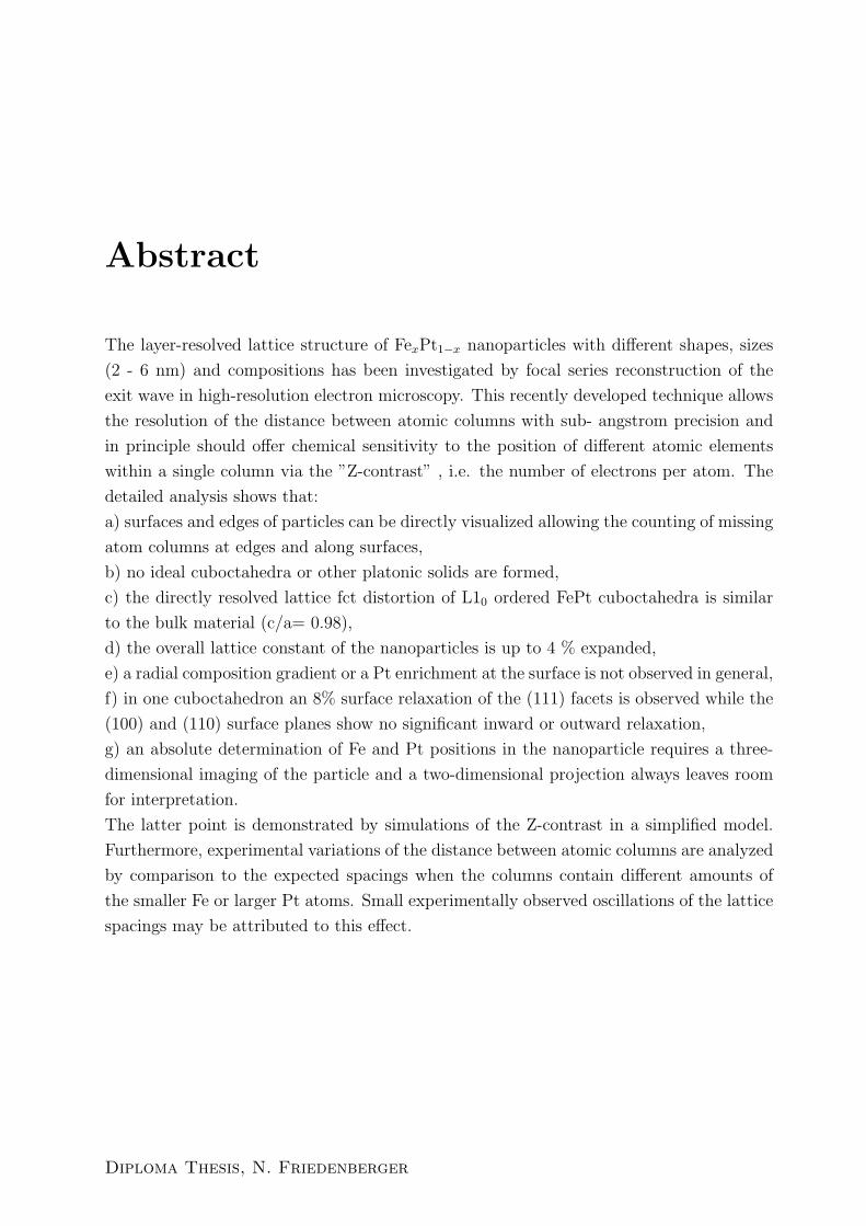
be the origin of those changes in the orbital magnetic moment. Figure 1.2 shows different
chemical distributions of Fe and Pt atoms in a NP and suggests that the lattice constant
and the lattice spacing, respectively, might not be unique throughout the particle and
therefore will definitely influence the orbital magnetic moment. Another interesting ques-
tion in that context is how a radial composition gradient or a shell-wise layered structure
have an influence on the lattice parameter in a NP. The experimental investigation of these
effects was the aim of this thesis. Therefore recently introduced High Resolution Transmis-
sion Electron Microscopy (HR-TEM) techniques which allow the determination of lattice
Layer resolved Lattice Relaxation in Magnetic FexPt1−x Nanoparticles
7
Figure 1.2: This figure shows 6 snapshots of the equilibrium structures of an equiatomic trun-cated cuboctahedron FePt-NP at different temperatures. White and dark circles represent Ptand Fe atoms, respectively [Yan05].
parameters of NPs with sub-Angstrom resolution [O´K01b] were applied. These techniques
were available at the National Center for Electron Microscopy in Berkeley (NCEM). In this
thesis I focussed on the following steps:
1. Sample Preparation for HR-TEM
2. HR-TEM-Analysis in Berkeley (National Center for Electron Microscopy) and in
Duisburg
3. Exit Wave Reconstruction of focal series HRTEM-images, which allows the retrieval
of the full phase and amplitude information of the electron exit wave.
4. Layer (atom column) resolved evaluation and interpretation of data
5. Image simulations to verify the results
In chapter 2 the main aspects of the theory of HR-TEM are summarized in short. The
method of Exit-Wave-Reconstruction (EWR) is explained, and the process of image sim-
ulation is described. It is shown that EWR is the only feasible method yielding chemical
sensitivity with sub-Angstrom resolution. After the theoretical description of the funda-
mentals several preparation methods for the NPs investigated in this thesis are shortly
described. Finally the layer resolved analysis for chemically and gas-phase prepared NPs
is discussed in detail. It is shown that under specific conditions a correlation with the
Diploma Thesis, N. Friedenberger

8 Introduction
measured lattice relaxation and the chemical order within the atomic planes and columns
can be deduced.
Layer resolved Lattice Relaxation in Magnetic FexPt1−x Nanoparticles
Chapter 2
Basics
This chapter gives an introduction to the theory and functionality of High Resolution
Transmission Electron Microscopy. Since image simulations are required for quantita-
tive interpretations of HR-TEM-images the main aspects are presented in section 2.1.5.
Yet the main focus of this chapter will be the explanation of the method of Exit-Wave-
Reconstruction to achieve sub angstrom resolution. A theoretical overview concerning the
idea and concept of EWR is given in 2.2.2. A short manual for the TrueImage software
which was used for EWR can be found in Appendix A-5.
2.1 Theory of HR-TEM
The theory of (High Resolution) Transmission Electron Microscopy has been described in
many textbooks [Rei84, Wil96]. Here only the most important facts only will be presented
to understand HR-imaging.
Using electrons for microscopy yields smaller wavelengths and therefore a higher resolu-
tion. Theoretically, the resolution is 5 times higher than for visible light. For a 300kV
(λ = 1.97pm) electron microscope the point-resolution should be in the range of 1 pm, for
example, according to the Rayleigh criterium [Wil96]. The typical (point) resolution of a
present TEM is worse than the calculated wavelength of the electrons. The attainable reso-
lution of a transmission electron microscope (TEM) is mainly determined by the properties
of the objective lens. One major lens defect, called spherical aberration and characterised
by the spherical aberration coefficient, CS, causes rays or electrons away from the optical
axis not to be focused on the same focal point as those propagating on the optical axis
[Sch05]. Nowadays, the highest achieved resolution is 0.78 Angstrom in Si [112] [Kis06a].
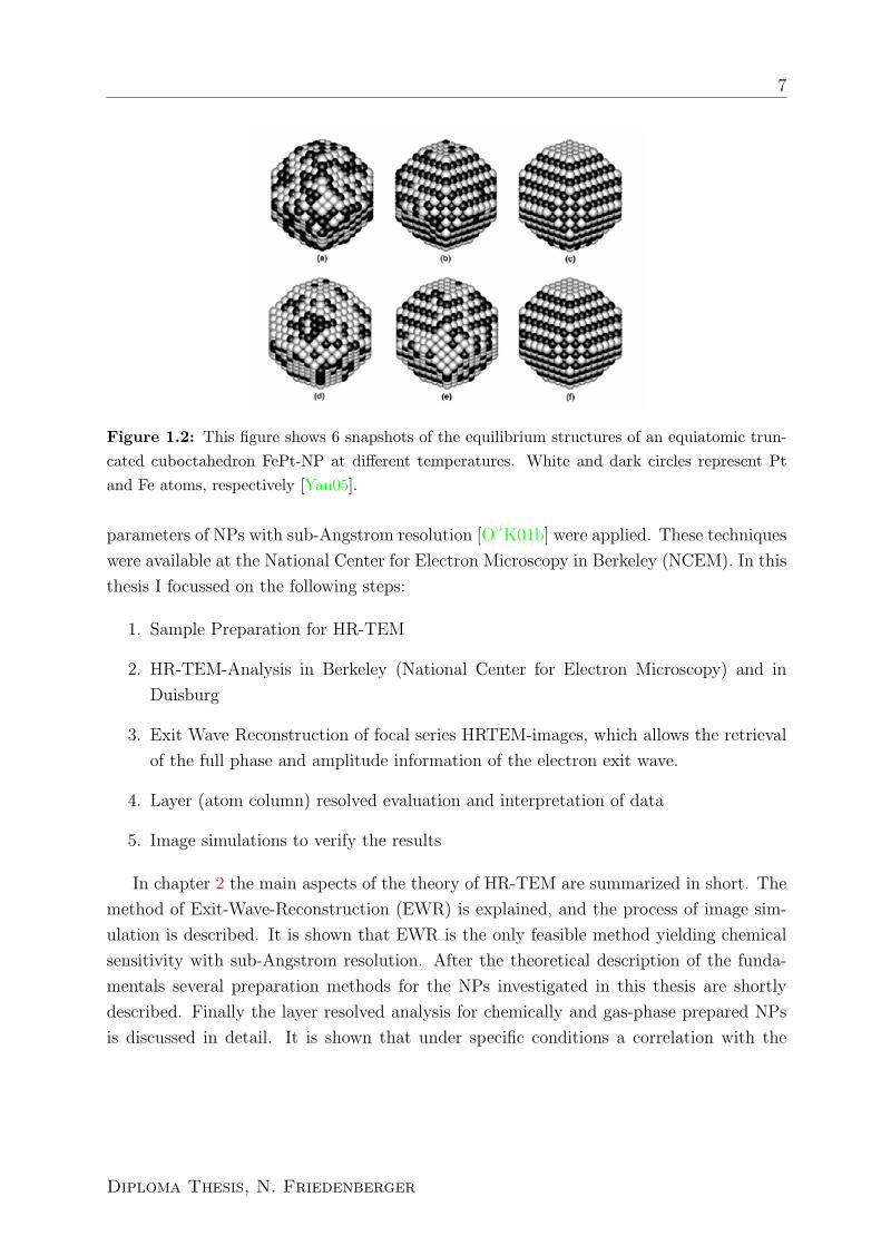
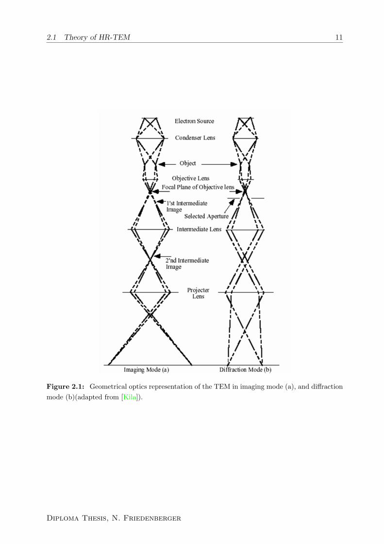
Fig. 2.1 shows the geometrical optics in a Transmission electron microscope (TEM) in
Diploma Thesis, N. Friedenberger

10 Basics
imaging (a) and diffraction mode (b).
2.1.1 Principle of High Resolution - Phase Contrast
There are in general three different contrast mechanisms in TEM. The mass-thickness
contrast, the diffraction contrast and the phase contrast. In general the contrast, abbr.:
(C), can be defined as the difference of the intensity (∆I) between two adjacent areas I1
and I2 [Wil96]:
C =(I1 − I2)
I1=
∆I
I1(2.1)
The phase contrast arises due to the differences in the phase of the electron waves
scattered through a thin specimen to which the weak phase object approximation (WPOA)
can be applied. This contrast mechanism is sensitive to many influencing factors like
thickness changes of the specimen or astigmatism of the objective lens. Therefore the
images are not easy to interpret. The phase contrast offers an improved sensitivity for
the analysis of the atomic structure of thin specimens [Wil96]. For phase imaging several
scattered electron beams contribute to the image and need to be properly reconstructed.
In this context another aspect has to be mentioned, the appearance of lattice fringes in High
Resolution TEM. In [Wil96] the origin is described using a simple two beam approximation.
The result shows that the intensity varies sinusoidally with different periodicity for different
values of g′. g is the diffraction vector for the corresponding diffracted beam and g
′= g+sg,
where sg = excitation error. With care the fringes can be related to the spacing of the
lattice planes normal to g′keeping in mind that they are not direct images of the structure
itself! Nevertheless, they can give lattice spacing information.
Image information - Amplitude-Phase-Diagrams
Taking into account the scattering cross-sections of the electron wave with the atomic
potentials of the specimen and the interference of several beams it is possible to achieve
atomic resolved information as described in section 2.1.1. Electron waves of the form:
Ψ = A exp(iφ) are fully described by their amplitude and phase.
However, in the TEM one measures intensities only. The amplitude and phase information
is lost. Therefore the technique of reconstructing the electron exit wave was developed, see
section 2.2.2. The electron exit wave is the wave directly below the sample plane. It only
contains the information of the sample and is not modified by lenses. Unfortunately, the
electron exit wave cannot be detected directly. It propagates through the optical system
Layer resolved Lattice Relaxation in Magnetic FexPt1−x Nanoparticles
2.1 Theory of HR-TEM 11
Figure 2.1: Geometrical optics representation of the TEM in imaging mode (a), and diffractionmode (b)(adapted from [Kila]).
Diploma Thesis, N. Friedenberger

12 Basics
of the microscope until reaching the screen or CCD camera. Both, the imaging system
and the detection system influence the electron exit wave so that the acquired image has
lost part of its information. These effects are mathematically described by the contrast
transfer function (CTF) described in the next section 2.1.3.
If full phase and amplitude information are known, they can be presented in a polar plot:
amplitude-phase diagrams, also called Argand plots. In these diagrams the amplitude
defines the length of the vector and the phase is represented by the polar angle.
2.1.2 Analyzing Images - Delocalization and Resolution
The point of interest in acquiring and quantitatively analyzing HRTEM-images is the
separation of individual atomic columns. Typically, lattice fringes are observed with high-
resolution transmission electron microscopy (HR-TEM). But the direct imaging of the
lattice structure of 2 to 6 nm sized nanoparticles is often disturbed by aberration and
delocalization effects. The difficulty in imaging interfaces or surfaces is to judge where
the interface is exactly located, because the information is spreading over a larger area
(compare fig. 2.2 [Gro99, Sch05]). This so-called delocalization is due to a non-zero CS
value. The electrons from one point of an object are not imaged into a single point but
rather into a small disk smearing out the information (the information is no longer localized
but delocalized).
Artifact-free imaging and ultimate resolution is possible by reducing the main lens
defects either by software or by hardware. The hardware is featured by integrating new
electron-optical components like monochromators or CS correctors into the microscope.
The TrueImageTM software obtains directly interpretable results from high-resolution TEM
beyond the point-resolution. This reconstruction mathematically eliminates the spherical
aberration of the microscope, thus removing delocalization effects from the FEG electron
source and therefore it is a very good alternative compared to working with the new
generation of microscopes, the Cs aberration-corrected TEMs. And please note that even
in an hardware corrected microscope it is still beneficial to make EWR in order to recover
the exit wave from the image intensities [Jin02].
Resolution up to the information limit of the microscope is achieved by applying an special
algorithm to the images which are acquired in focal series. In this process lens aberrations
and delocalization are compensated and the resolution of the microscope can be pushed to
the information limit. First sub-Angstrom resolution was reported in [Kis]. For the OAM
(One Angstrom Microscope) it is 0.8 A [O´K01b].
Layer resolved Lattice Relaxation in Magnetic FexPt1−x Nanoparticles

2.1 Theory of HR-TEM 13
Figure 2.2: Image of Au particles on carbon support film. With an uncorrected objective lens(a) strong delocalization (fringe contrast outside the particles) is visible. In the CS-corrected case(b) the delocalization has disappeared and the Au particle is imaged artifact free [Sch05].
2.1.3 Contrast Transfer Function
The optical system of the microscope transforms each point of the specimen into a disk1
in the final image. This is described by the point spread function h(r). The final image is
a convolution of the point spread function with the specimen transmission function (exit
wave)f(r). The realspace convolution is difficult to treat mathematically. The problem is
fourier transformed to the reciprocal space and the convolution becomes a simple multi-
plication. The Fourier transformed point spread function is the so called contrast transfer
function (CTF) H(k). k is the spatial frequency, sometimes in literature, e.g. [Wil96],
also referred to as u or in chapter 2.1.4 as G. The spatial frequency corresponds recipro-
cally to distances, high spatial frequencies mean small distances and vice versa. Therefore
large spatial frequencies are needed for high resolution.
The following phenomena contributes to the CTF: apertures, attenuation of the wave and
the aberration of the lens. They are described by the aperture function A(k), the envelope
1 The radius of the point spread area is given by [Lic91]:
ρ = −0.75CS(dχ
dk)max (2.2)
With the aberration function and phase distortion function respectively χ(k).
Diploma Thesis, N. Friedenberger

14 Basics
function E(k) and the aberration function B(k). The CTF can be written as following:
H(k) = A(k)E(k)B(k) (2.3)
The aberration function is of an exponential form:
B(k) = exp(−iχ(k)) (2.4)
With the so called ”phase grating” function χ(k) which has the form of a phase shift
expressed as 2πλ
times the path difference traveled by the spherical aberration, defocus and
astigmatism affected waves [Wil96]:
χ(k) = π∆fλk2 +1
2πCSλ
3k4 (2.5)
The former mentioned weak phase object approximation (WPOA), which uses a two
dimensional projection of the crystal structure to represent the potential of the specimen,
reveals that for a very thin specimen the amplitude of the transmitted wave function is
linearly related to the potential [Wil96]. This approximation yields for the electron exit
wave:
f(x, y) = 1 + iσVt(x, y) (2.6)
where Vt(x, y) is the projected potential in z-direction and σ a interaction constant.
Using this approximation, the correlation of the electron exit wave function with the CTF
and the fact that the intensity is given by:
I = ψψ∗ =| ψ |2 (2.7)
and neglecting terms in σ2 because σ is small, the following expression is obtained:
I = 1 + 2σVt(x, y)⊗ sin(x, y) (2.8)
This shows that only the imaginary part of the aberration function B(k) contributes
to the intensity so that equation 2.4 can be set to:
B(k) = 2 sin(χ(k)) (2.9)
Using this expression for B(k) a new function, the transfer function T (k) can be defined:
T (k) = A(k)E(k)2 sin(χ(k)) (2.10)
Layer resolved Lattice Relaxation in Magnetic FexPt1−x Nanoparticles
2.1 Theory of HR-TEM 15
which is often called the contrast transfer function, too. This sinusoidal expression for
the CTF is also used for the plots made with the CTF-explorer [Sid] in this thesis.
Information limit
The information limit is a microscope-specific parameter and gives the maximum resolution
which can be achieved with the instrument. It is defined as the spatial frequency from which
the CTF oscillations are equal to the noise level and the envelope functions damp the CTF
to zero, respectively [Sid].
Point-to-point resolution
The point-to-point resolution for one defocus value is the spatial frequency or rather the
resolution for which the corresponding CTF has its first node. Images with only smaller
spatial frequencies2 are directly interpretable since the contrast is of the same sign in that
area. For spatial frequencies larger than the first-node value the contrast is not directly
interpretable and image simulations are needed, see chapter 2.1.5. Negative values of the
CTF and the phase transfer function respectively correspond to a positive phase contrast,
which makes atom columns look dark and the background look bright, and vice versa for
positive values [Sta03b]. The defocus which yields the largest point-to-point resolution is
called Scherzer defocus and defines the point-to-point resolution of the microscope.
Optimum defocus
Finding the optimum defocus is difficult. Equation 2.10 gives only one free parameter
to optimize the CTF which is the defocus value. Which defocus is optimum depends on
what is to be achieved. If one wishes as good a resolution as possible or if one wants
directly interpretable images makes a difference in the choice of defocus. As described in
the section 2.1.3 the Scherzer defocus given by equation 2.11 yields the best results for the
direct interpretation of images but at the expense of the resolution.
∆fScherzer = −1.2√CSλ (2.11)
Especially for layerwise investigations of atom columns in nanoparticles it is necessary
to have a resolution up to the information limit of the microscope which is not the case for
working under Scherzer defocus conditions, see fig. 2.3 for the Scherzer defocus.
In [Lic91] Lichte presents some theoretical results concerning the optimum focus for taking
2which can be achieved by using apertures to cut the larger spatial frequency values
Diploma Thesis, N. Friedenberger

16 Basics
electron holograms. He found an optimum defocus for the desirable value of the maximal
spatial frequency, the information limit. His calculation includes the assumption that by
subsequent reconstruction the aberrations of the objective lens will be corrected. This
optimum defocus value is nowadays known as the Lichte defocus and given by:
∆fLichte = −0.75CS(kmaxλ)2 (2.12)
The idea of his investigations was to minimize the derivative dχdk
and to choose the
defocus values which minimizes the maximum value of the modulus of the derivative of
the wave aberration function χ(k) respectively [Lic91], for the spatial frequency interval of
interest (0 − kmax). This corresponds to minimizing the radius of the point spread area,
as can be seen in equation 2.2.
Summing up this section there is to say that the Lichte defocus is the best in terms of
obtaining the highest info limits while the Scherzer defocus yields the best point-to-point
resolution. The problem of the Scherzer defocus is the number of nodes of the CTF which
mean no contribution of the corresponding spacial frequencies to contrast. Full recovery
of the information is possible by acquiring a so called focal series which is explained in
section 2.2.2.
Layer resolved Lattice Relaxation in Magnetic FexPt1−x Nanoparticles

2.1 Theory of HR-TEM 17
Figure 2.3: Scherzer and Lichte defocus for the CM300 microscope. The upper x-axis gives thereal space dimension in nm.
Diploma Thesis, N. Friedenberger
18 Basics
2.1.4 Sample Wave Interaction - HR-TEM Image Formation
Interpreting HRTEM-images is not easy, because in most cases the images are anything
but a direct structure representation of the sample. Due to the interaction of the electrons
with the specimen a complicated interference pattern of diffracted electron beams and the
central beam φ(G)3 is formed which includes linear and non-linear effects. This short
theoretical overview is adapted from [Coe96] and [Ish80] and uses the same notation as in
the EWR-chapter 2.2.2. A more detailed theoretical discussion of image formation can be
found elsewhere, e.g.[Wil96, Rei84].
According to [Ish80] the diffracted electron beams result in the spatially varying image
intensity in the image plane with the general Fourier components I(G). G is the two-
dimensional spacial frequency vector. Under isoplanatic imaging conditions and with T,
the transmission-cross-coefficient, I(G), the image intensity fourier coefficient, is given by:
I(G) =∫φ(G + G
′)φ∗(G
′)T(G + G
′,G
′)dG
′(2.13)
Eq.2.13 can be treated separately for the two cases G 6= 0 (”ac”-component) and G = 0
(”dc”-component4).
I(G = 0) =∫|φ(G
′)|2dG′
”dc” component (2.14)
I(G 6= 0) = φ(0)φ∗(−G)T(0,−G) + φ∗(0)φ(G)T(G, 0)
+∫G′ 6=0;G′ 6=−G
φ(G + G′)φ∗(G
′)
×T(G + G′,G
′)dG
′”ac” component (2.15)
φ(G = 0) is the transmitted electron beam and φ(G 6= 0) is one of the diffracted beams.
While in equation 2.15 in the first two terms the information of the linear interferences
between the transmitted electron beam with one diffracted electron beam is given, the
third term accounts for non-linear interferences between diffracted electron beams. The
3note that the spatial frequency G was denoted by k in chapter 2.1.34spatially constant, non varying
Layer resolved Lattice Relaxation in Magnetic FexPt1−x Nanoparticles

2.1 Theory of HR-TEM 19
Transmission-Cross-Coefficient (TCC) takes into account aberrations and coherence effects
and is expressed by:
T(G1,G2) = p(G1)p∗(G2)E∆(G1,G2)ES(G1,G2) (2.16)
with p(G) denoting the pure phase transfer function (PTF) equation 2.17, E∆ and
ES being envelopes for temporal (δ) and spatial (S) coherence. E∆(G1,G2) is influenced
by the defocus of the objective lens (∆f) and the ”focal spread” parameter (∆) whereas
ES(G1,G2) is dependent on the electron wavelength λ and α denotes half the angle of
beam convergence.
p(G) = exp[−2πiχ(G)] (2.17)
χ(G) is the aberration function of the electron wave. It describes phase distortions due
to the spherical aberration, represented by the aberration coefficient CS, and the defocus
value ∆f :
χ(G) =1
2∆fλG2 +
1
4CSλ
3G4 (2.18)
This expression is also known from chapter 2.1.3. Specially for a FEG-TEM according to
its high spatial coherence T(G1,G2) can be factorized, so that:
T(G1,G2) ≈ t(G1)t∗(G2)E∆(G1,G2) (2.19)
with t(G) being the effective transfer function (product of pure transfer function and the
linear envelope function):
t(G) = p(G)ES(G, 0) = exp[−2πiχ(G)]×[−
(πα
λ
)2
[∇χ(G)]2]
(2.20)
For this factorization approximations had to be made. There occurs an error for most of
the non-linear interferences, which can be neglected for a FEG due to not causing huge
offset errors in the model used for the image reconstruction. For larger values of α this
approximation has to be improved.
There is also blurring of the image due to the detection process. To model this effect
a damping function is used which acts on the frequency components of the ideal image
intensity. This ”damping envelope” is given by 2.21. ID(G) is the modelled image intensity
for all blurring aspects. Those of the detection process are the modulation transfer function
Diploma Thesis, N. Friedenberger

20 Basics
of the detector (CCD camera) M(G) and two envelopes for vibration V(G) and drift D(G)
of the sample during the image acquisition.
ID(G) = EI(G)I(G) (2.21)
EI(G) = M(G)V(G)D(G) (2.22)
2.1.5 Image Simulation
For reasonable HR-TEM-image interpretation it is absolutely necessary to do image simu-
lation (see also [Dmi03]), i.e. all possible models of the structure have to be simulated by
computers. Comparing the simulated images with the experimental data will help to find
the real structure of the sample. But this is to be considered very carefully. Only if really
all thinkable model-structures have been simulated as well as the simulation parameters
have been chosen very sensibly, the right interpretation of the HRTEM-images becomes
possible. It is also a good idea to match simulation and experimental data for different
orientations.
Different approximations
The scattering behavior of an electron wave propagating through a crystal structure is fully
described by the Schroedinger equation. Since it is still difficult to solve even in the so called
forward scattering approximation, Cowley and Moodie (1957) developed the Multislice
Method which is much more elegant [Cow57]. There also exists another approximation
in terms of Bloch waves. Here the electron wavefunction as a function of the reciprocal
space vector k is written as a linear combination of Bloch waves b(k, r) with coefficients
ε (Howie, 1963 [How63]). Each Bloch wave is itself expanded into a linear combination
of plane waves which reflect the periodicity of the crystal potential. That leads to a set
of linear equations to be solved. The Bloch wave approximation can be characterized as
follows:
• Easy accounting of reflections outside the zero order Laue zone, but also requires
exact specification of which reflections g are included in the calculation.
• Very good for perfect crystals, but not suited for calculating images from defects.
• Validity of the solution for a particular specimen thickness.
• Dynamical scattering is included.
Layer resolved Lattice Relaxation in Magnetic FexPt1−x Nanoparticles

2.1 Theory of HR-TEM 21
• Allows rapid calculation of convergent beam electron diffraction patterns.
The Multislice Approximation
The idea of the Multislice Method is to ”cut” the sample perpendicular to the incident
electron beam into slices. For every slice the crystal potential is projected to a plane. Thus
the electron wavefunction is calculated at z+n∗dz by taking the output of one calculation
as the input of the next one.
Ψ(x, y, z + dz) ≈ exp[−iσdz∇2x,y] · exp[−iσ
∫ z+dz
zV (x, y, z
′)dz
′]Ψ(x, y, z) (2.23)
This equation is solved in a two step process. The potential due to the atoms in a slice
dz is projected onto the plane t = z, giving rise to a scattered wavefield:
Ψ1(x, y, z + dz) = exp[−iσ∫ z+dz
zV (x, y, z
′)dz
′]Ψ(x, y, z) ≡ q(x, y)Ψ(x, y, z) (2.24)
where the function q(x, y) is referred to as the phasegrating.
The wavefield is propagated through vacuum to the plane t = z + dz:
Ψ(x, y, z + dz) = exp[−iσdz∇2x,y] ·Ψ1(x, y, z) (2.25)
This equation being a convolution in real space is therefore transformed to the Fourier
space:
Ψ(H, z + dz) = exp[−iπλdzH2] ·Ψ1(H, z) ≡ p(H, dz) ·Ψ1(H, z) (2.26)
with Ψ(H, z) being the Fourier coefficients and the so called propagator p(H, dz). A
repeated use of the last two equations defines the multislice formalism giving the wavefield
at any arbitrary thickness T of the specimen.
Image formation
In this section the image formation by a simulation Software is described in accordance
to [Kila]. Only the first lens of the microscope, the objective lens, is considered in the
simulation calculations. All the other lenses just magnify the image formed by the objective
lens. Since the angle which the electrons form with the optic axis of the lens varies inversely
with the magnification, only the aberrations are important. Without any aberrations,
Diploma Thesis, N. Friedenberger

22 Basics
instabilities and with the specimen in the focal plane of the objective lens, the image
observed in the microscope would be a magnified version of:
I(x, y) = |Ψ(x, y, z = exitplane of specimen)|2 = Ψe(x, y)Ψ∗e(x, y) (2.27)
Normally, the following effects are included in the calculation:
• spherical aberration
• chromatic aberration
• lens defocus
• considered correctable by the operator, but can also be included in the equations:
– two-fold astigmatism
– three-fold astigmatism
– axial coma
Considering only spherical aberration and defocus of the objective lens, the image would
be obtained as follows:
1. Calculate the wavefield emerging from the specimen according to one of the approx-
imations.
2. Fourier transform the wavefield which gives the amplitude and phase of scattered
electrons.
3. Add the phase shift introduced by the lens defocus and the spherical aberration to
the Fourier coefficients.
4. Inverse Fourier transform to find the modified wave function.
5. Calculate the image as the modulus square of the wavefield.
However there are two more effects concerning variations in electron energy and di-
rection to be considered: chromatic aberration/temporal incoherence and beam diver-
gence/spatial incoherence. The chromatic aberration causes electrons of different energies
to focus on different planes. Therefore a Gaussian spread in defocus is assumed in the
calculation which leads to a damping of each Fourier term (diffracted beam). Another
damping of the diffracted beam occurs due electrons not proceeding parallel to one an-
other, thus forming a cone of an angle α. This leads to a disk instead of a point in the
diffraction pattern.
Layer resolved Lattice Relaxation in Magnetic FexPt1−x Nanoparticles
2.2 Different Applications of HR-TEM 23
Stobbs factor
The Stobbs factor is a factor describing the ratio of contrast in simulated and experimental
images and is defined as follows:
Stobbs factor =contrast in simulated image
contrast in experimental image
The typical value of the Stobbs factor is 3. Still nowadays the origin of this big difference
is not explained and under intensive investigation. There were some thoughts including
a frozen phonon approach yielding results which were even worse according to the ex-
perimental data. C. B. Boothroyd ascertains the problem, see [Boo00] for example. He
has also performed some investigations on phonon scattering influencing the experimental
measured intensity. There are 2 methods to get access to phonon scattering. They are
described in [Boo03] and in [Boo05]. Summarizing those experiments yielded an influence
of 10− 15% which does not explain the discrepancy between simulated and experimental
images either. According to Boothroyd there must be other reasons for the Stobbs factor
which he sees in the part dealing with microscope parameters of simulation calculations.
2.2 Different Applications of HR-TEM
Transmission Electron Microscopy offers many possibilities of characterizing materials.
In this thesis the so called CTEM (Conventional Transmission Electron Microscopy) was
mainly used. For the chemical analysis the analytical TEM (ATEM) is used which employs
the techniques of electron energy loss spectroscopy (EELS) and the energy dispersive x-ray
spectroscopy (EDS). EDS is a common method to characterize thin films and particles
by element specific energy spectra generated by X-rays from scattering processes of the
electron beam-sample interaction. In the electron energy loss spectroscopy (EELS) the
energy of the inelastic scattered electrons is detected.
Since the aim of this thesis was to analyze the lattice structure of the FePt-nanoparticles
lattice imaging had to be processed which means HR-TEM had to be done. As described
in 2.1.4 aberrations and delocalization effects (2.1.3) influence the image and have to be
considered when interpreting the results. So the goal was to find a way of minimizing
this disturbing effects but simultaneously to maximize the information. The maximum
information is obtained when the amplitude and phase of the electron is detected. And the
maximum also means to extend your information up to the limit of the microscope, the
information limit (2.1.3) which is given by mechanical limitations of the microscope. So the
Diploma Thesis, N. Friedenberger

24 Basics
idea of Exit Wave Reconstruction was born. Because HR-TEM images only show a two-
dimensional projection of the sample, it is not possible to get any three-dimensional (3D)
shape information. Hence another technique is necessary: 3D-Tomography (e.g. [Bal06]).
2.2.1 Quantitative HR-TEM
The Z-contrast is the dependence of the image ”intensity” from the atomic number Z(I ∼Z2). That means ”heavier” atoms contribute more to contrast than ”lighter” atoms. In
TEM the Z-contrast is usually used in the Scanning Transmission mode (STEM - Scanning
Transmission Electron Microscope) because in this mode the beam is focused to a single
spot of the sample. In HR-TEM a parallel illumination is used. If Scherzer imaging is
applied atom columns appear black in HR-TEM while they appear white in STEM. With
the introduction of EWR the phase problem was solved and a quantitative interpretation
of image intensities became possible in HR-TEM.
Fig. 2.4 shows the Z-dependence of the signal/noise ratio for HR-TEM and STEM
for single atoms. It is clear that HR-TEM exhibits a larger signal/noise ratio over the
whole Z-range. In 2002 one could expect to detect single atoms in HR-TEM for Z larger
than 2 and STEM single atoms with Z larger than 40. The strength of STEM is a better
discrimination of atoms with different Z. The current development of hardware CC and CS
correctors in essence aims at an improvement of signal/noise ratios (detection limits) for
STEM and HR-TEM.
In STEM the chemical sensitivity originates from Rutherford scattering. In HR-TEM
the origin of chemical sensitivity is illustrated in fig. 2.5. There the zero beam is plotted as
a function of sample thickness and for different elements of atomic number Z. An identic
cubic structure is considered in all cases. It is seen that the beam intensity oscillates with
sample thickness. The periodicity of these oscillations is called extinction distance. The
extinction distance decreases with increasing Z. Moreover, gray values repeat periodically
as a function of sample thickness and uniqueness requirements make it often necessary to
restrict measurements to a thickness limited by the first extinction oscillations. Please note
that in crystals made from heavy materials this thickness can be very small.
Layer resolved Lattice Relaxation in Magnetic FexPt1−x Nanoparticles

2.2 Different Applications of HR-TEM 25
Figure 2.4: Sensitivity of Exit Wave Reconstruction (diamond), and HAADF imaging for thedetection of single atoms with atomic number Z (13). A signal to noise ratio of 1 is consideredto be the detection limit [Kis02].
Figure 2.5: Zero beam intensity versus sample thickness of a fcc crystal with lattice parametera=0.4 nm and lattice sites occupied by the indicated elements [Kis02].
Diploma Thesis, N. Friedenberger

26 Basics
2.2.2 Exit Wave Reconstruction
The idea of Exit Wave Reconstruction is to remove all the blurring effects in the exit wave
caused by the imaging system of the microscope and to reconstruct the ”image” directly
below the sample. This task requires a physical description of the model ”reconstruc-
tion” and also demands to reconstruct from a series of intensity images the amplitude and
phase contrast of the exit wave. In the intensity image, given through Ψ2, the phase and
amplitude information is completely lost. The most important work enabling a complete
reconstruction of the Exit-Wave was done by Kirkland [Kir84] and Thust [Thu96],[Coe96].
Why focal series acquisition?
For Exit-Wave-Reconstruction the acquisition of a focal-series is required. But why is
this the way of choice to recover the complete electron exit wave information and what
is a focal series? The Contrast Transfer Function is ”responsible” for the information
transfer from the Exit-Wave of the sample to the image as already discussed in 2.1.3.
The problem is, that the CTF oscillates heavily for higher spatial frequencies, especially
for the microscopes using a Field Emission Gun (FEG). And those oscillations mean no
spatial frequency information for the crossing points with the x-axis. To recover all spatial
frequencies and the full phase information a series of images must be recorded with different
focus settings. Focal series means a series of images taken under identical conditions in the
microscope apart from the defocus value which is changed by a small fixed amount for every
acquisition. As shown in 2.6 changing the defocus value by 4 nm only causes a slight shift of
the CTF for the higher spatial frequencies. For a shift in the low frequency area the defocus
change has to be larger. 2.7 shows 3 direct comparisons of a -270 nm defocus with -2 nm,
+10 nm and +20 nm deviating defocus values. It is easy to see that a defocus change of 20
nm only leads to a slight change of the lower spatial frequencies. Therefore it is necessary
to use a larger defocus range, e.g. 40 nm. With a defocus step of 2 nm this leads to a series
of 20 images which is a typical number. Due to the fact that the delocalization effects
2.1.2 are smallest for the Lichte-defocus as shown in 2.1.3 it is consequentially that a focal
series is taken around Lichte-defocus. For the CM300-microscope which was used for my
investigations Lichte-defocus is -273 nm and that is why the defocus values in 2.6 and 2.7
are chosen around -270 nm. According to [Kis06a] other defocus values were discussed in
order to extend the resolution. Both an aberration free defocus and an alpha-null defocus
were suggested to optimize information transfer for Exit Wave Reconstruction [O’K01a].
However, there were many obstacles like inability to predict image Fourier components for
non-periodic structures and huge image delocalization which still make the Lichte defocus
Layer resolved Lattice Relaxation in Magnetic FexPt1−x Nanoparticles

2.2 Different Applications of HR-TEM 27
the best for focal series recording.
Different methods of image processing
The imaging process can be considered approximately linear for very thin samples. For
this linear model a closed form image reconstruction solution exists. On the other hand,
for thicker samples it is necessary to work with a non-linear model. Kirkland presented in
[Kir84] a method of nonlinear image reconstruction from a defocus series which is based
on the maximum a-posteriori method (MAP) of image restoration. But this method only
works with one image. Kirkland names his new method multiple input MAP (MIMAP).
It provides refining of the defocus values, translational alignment of the images of the
series and is general enough to improve the non-linear partial coherence reconstruction
theory for which a approximate formulation has been published before. In [Kir84] two
different approaches to the MIMAP reconstruction are discussed: one using fast fourier
transforms (FFT) based on an approximation to the spatial coherence which uses less
computer time; the other one is more precise but therefore it needs much more computer
time. In Kirkland’s MIMAP method a least-square functional is minimized and so the
electron wave is matched to the measured intensities of the focal-series. Based on his
pioneering work in the area of non-linear image reconstruction improved versions have been
developed by Coene at al. [Coe96]. This was necessary because it was demonstrated that
MIMAP only worked for a few images of a very limited frame size. Another disadvantage
was the long computation time due to the 50-100 iterations which are necessary to reach
convergence. The method developed by Coene et al. is called maximum-likehood method
(MAL). It uses a least-square functional similar to the one in MIMAP. The difference
between the two methods is a noise-control term containing a priori information on the wave
function which is used in MIMAP but not in MAL. The coupling of the wave function and
its complex conjugate (in HR-TEM image formation and the exit wave reconstruction)is
also considered in the MAL approach . Another item deals with the optimization of the
numerical implementation for large frame sizes which are typical for slow scan CCD cameras
(512×512 pixel2, 1024×1024 pixel2). A large frame size of the images is necessary because
a real space sampling interval of sub angstrom size is required. That leads to a field of
view of 12nm in a frame of 512 × 512 pixel2. Also not to be neglected is the influence of
the point-spread function which effects a smaller effective field of view. In addition to the
MAL-approach which was developed in the BRITE-EURAM project there exists another
concept also developed in the same project. This so-called paraboloid concept deals with
the linear processing of the reconstruction but yields two improvements compared to former
Diploma Thesis, N. Friedenberger

28 Basics
Figure 2.6: CTF for two different defocus values. Plotted with CM300 parameters. The redarrow indicate the information limit of the CM300. The spatial frequency k is the same as onedenoted with G in the text. The upper x-axis gives the real space dimension in nm.
Layer resolved Lattice Relaxation in Magnetic FexPt1−x Nanoparticles

2.2 Different Applications of HR-TEM 29
Figure 2.7: Comparisons of the CTF for a defocus of -270 nm and -272 nm, -260 nm and -250nm. Plotted with CM300 parameters. One should note how sensitive the CTF reacts for spatialfrequencies G = k > 0.14.
Diploma Thesis, N. Friedenberger

30 Basics
linear approaches for which a strong beam had to be assumed: (i) weighting linear and non-
linear terms properly leads to a constant determination of the beam amplitude (ii) treating
of non-linear terms as a perturbation −→ recursive application of the linear reconstruction
scheme. This paraboloid method (PAM) also known as ”Van Dyck method” is related to
early work by Saxton whereas the maximum-likehood method is based on Kirkland’s work
as elucidated before. According to Coene [Coe96] the reconstruction performance of MAL
is superior to that of PAM.
In 2.8 a typical ”mean squared difference” convergence plot is shown as a function of
the number of iterations. It points out that a combination of PAM and MAL leads to
the best results concerning convergence and iteration time. The advantage of PAM is that
it converges very fast, MAL on the other hand allows for a better solution because this
method uses all information of the images optimally. Using only the MAL iterations would
require many more iterations to get the same result than the combination of both yields
[Dyc96].
The MAL method
HRTEM image reconstruction is used to calculate the electron wave φ at the specimen
exit plane. This is usually done by minimizing an error functional over a focal series of N
images.
S2 =1
N
N−1∑n=0
∫dG|δIn(G)|2 (2.28)
The mean-squared error S2 of the estimated images with respect to the experimental
images is given by equation 2.28. δIn(G) is the image difference for the nth focal image
(n = 0, ..., N − 1). With In,E, the intensity of the experimental and In,φ, the intensity for
a particular estimate of the electron wave φ simulated nth focal image:
δIn(G) = In,E(G)− In,φ(G). (2.29)
The recursive minimization process is based on the gradients of S2 with respect to the
related Fourier components of the electron wave. Hereby φ(G) and φ∗(−G) are equivalent
to φ∗(G) and φ(−G). The gradients are formally written as follows:
g(G) ≡ ∇φ∗(G)S2 (2.30)
g∗(−G) ≡ ∇φ(−G)S2 (2.31)
Layer resolved Lattice Relaxation in Magnetic FexPt1−x Nanoparticles

2.2 Different Applications of HR-TEM 31
Figure 2.8: Convergence of a simulation experiment of YBa2Cu4O8 with parameters for a 200kVFEG-TEM. The full line shows the convergence for only PAM iterations, the black dashed lineindicates the convergence for the first and second PAM-iterations and followed by MAL (after[Dyc96]).
Diploma Thesis, N. Friedenberger

32 Basics
For minimizing S2 eq. 2.30 and eq. 2.31 have to be zero. With the estimated image
intensity from eq. 2.16 and eq. 2.21 one obtains from eq. 2.30 [Coe96]. This leads to the
MAL-equations which are written as:
0 =N−1∑n=0
∫dG
′Tn(G
′,G)φ(G′)δIn(G−G
′)× EI,n(G−G
′) (2.32)
0 =N−1∑n=0
∫dG
′Tn(−G,−G
′)φ∗(−G′)× δIn(G−G
′)EI,n(G−G
′) (2.33)
This MAL-equations determine how δIn, the difference between an experimental and an
estimated image, has to be fed back to the starting point to obtain an optimized recon-
structed electron wave φ.
Figure 2.9 shows the recursive scheme of the MAL procedure for one iteration step j −→j+1. The input are N(0 · · ·N−1) images of a focal series. The output is the reconstructed
electron exit wave φfinal after convergence has been reached. For a more mathematical in-
formation concerning the minimization of the least square functional [Coe96](section 4)
is the article of interest. The MAL-procedure for one feedback step can be described as
follows:
1. HR-TEM-images are simulated with the parameters of the microscope: e.g. defocus
spread, have to be well-known.
=⇒ estimated image In,φ (In,j for jth iteration) is received.
2. Comparison of estimated(In,j) and experimental (In,E) images.
3. Image differences δIn,j are computed
=⇒ tranformation of δIn,j to a correction δφj for the specimen wave φj
4. update to φj+1
5. . . . repetition of 1.− 4. (one feedback-loop), if convergence is reached =⇒ 6.
6. stop of iteration processing =⇒ output of φfinal
Layer resolved Lattice Relaxation in Magnetic FexPt1−x Nanoparticles

2.2 Different Applications of HR-TEM 33
Figure 2.9: This graphic is in conformity to [Coe96]. Represented is one iteration circle j −→j + 1 of the MAL method for HRTEM image reconstruction. φj is the electron exit wave at thestart (j) and φj+1 at the end of this cycle.
Some remarks on the paraboloid (PAM) method
The PAM-is a special case of the so called SC-MAL (self consistent-MAL) method, which
is a special treatment of the MAL-equations. It is described by:
c0φ1(G) =
1
N
N−1∑n=0
Fn(G)In,E(G) (2.34)
c0 is a value of the central Fourier component of the electron wave. A comparison between
linear and expected non-linear terms allows for the determination of c0. In this case only
”dc” information in the initial electron wave is used. Herein the filter functions Fn(G) are
applied to the experimental image intensities. All in all this is only a good approximation
for thin samples, though. This was already mentioned in 2.2.2 when discussing linear
approximation approaches.
Another method which yields information on the phase retrieval is the off-axis holog-
raphy explained in [Dyc96].
Necessity of EWR and conclusion
Exit Wave Reconstruction enables the following:
Diploma Thesis, N. Friedenberger

34 Basics
Figure 2.10: This graphic by [Kis06b] illustrates clearly the advantage of EWR: On the left sidethe normal lattice image for a silicon nitride ceramic sample of 7nm thickness is shown (defocusvalue of -279nm). Too many image Fourier components lead to this complicated lattice structurewhich does not represent the real structure. The result of the EWR is shown on the righthandside. Here detailed structure information is available, Si- and N-columns can be identified. Thesmall white-framed square area shows a simulated image of the crystal structure.
• achieving for the information limit of the microscope
• removing delocalization effects
• correcting aberrations, astigmatism and coma
• receiving complete amplitude and phase information
Though this method was already developed more than 10 years ago it is still nowadays
the best method relating to the determination of lattice structures in very small features.
Layer resolved Lattice Relaxation in Magnetic FexPt1−x Nanoparticles

2.2 Different Applications of HR-TEM 35
Figure 2.11: Another example demonstrating the efficiency of EWR for a FePt particle with5-fold-symmetry. In the reconstructed phase image on the right hand side the atom columns areindividually resolved on an amorphous C-coated grid whereas they are not in the left image takenunder Scherzer defocus.
Diploma Thesis, N. Friedenberger


Chapter 3
Experimental Techniques
3.1 Preparation Methods of FePt-nanoparticles
In this section the two different preparation methods, gasphase condensation and organometal-
lic synthesis, for the FePt-nanoparticles used in this thesis are described. Another section
in this chapter deals with the development of a new TEM-Tomography holder and the
preparation of special TEM/FIM-samples. Field Ion Microscopy (FIM) is a method pro-
viding chemical sensitive analysis. It was planned to perform experiments in the TEM
to investigate the lattice structure and to analyze the same samples by FIM to reveal
atomically resolved chemical information. The sample preparation for such TEM/FIM-
investigations was never done before and could not be optimized during my thesis. The
FIM investigations will have to be performed in the near future.
3.1.1 Gasphase Condensation
This method is established very well in our group and only the most important facts
concerning my thesis are described. More information on the preparation of the FePt-
nanoparticles by gasphase condensation can be found in [Sta03c, Rel03]. Recent inves-
tigations on the influence of nitrogen to increase the degree of chemical order [ea04] are
discussed in [Dmi06c, Dmi06b]. The sputtering system was developed and built by S. Stap-
pert [Sta03b]. This system allows for gasphase condensation of nanoparticles and thermal
sintering of the particles in vacuum before deposition on a substrate. The system (fig. 3.1)
consists of a nucleation chamber, a sintering furnace and a deposition chamber.
The FePt-nanoparticles are produced by inert gas condensation in the nucleation cham-
ber: gasphase Fe- and Pt-atoms/ions are sputtered from a target and nucleate homoge-
Diploma Thesis, N. Friedenberger

38 Experimental Techniques
Figure 3.1: a) Simplified scheme of the sputtering system [Dmi03]. b) Sample holder developedin this thesis which allows a simultaneous deposition on tips, conventional TEM-grids and 4x4mm Si-substrates. The W-wires are used to fix the tips in the holes which is necessary becauseof the vertical built-in position of the virtual moveable sample holder on which this holder istightened in the deposition chamber. c) Picture of the sputtering system from [Sta03b].
nously due to the cooling in the nucleation zone which causes the supersaturation of metal
vapor. The continuous gas stream carries the particles through the sintering furnace where
temperatures up to TS = 1273 K can be produced. Afterwards they are thermophoretically
deposited onto the substrates. The chemical composition of the nanoparticles is approx-
imately the one of the target but can vary with different target thickness [Sta03b]. The
important parameters for the gasphase condensation method are:
p: the nucleation pressure.
fAr, fHe, (fN2): the gas flow rates for Ar and He (and N2) respectively.
PDC: the power of the sputter source.
tsputter: the sputtering time.
Layer resolved Lattice Relaxation in Magnetic FexPt1−x Nanoparticles
3.1 Preparation Methods of FePt-nanoparticles 39
TKS: the temperature of the cooling shield.
TP : the temperature of the sample holder.
Samples
The gasphase condensated particles investigated in my thesis were prepared by adding
nitrogen in the sputtering process to get single crystalline, mostly L10-ordered particles
[Dmi06c, Dmi06b]. The following parameters were used: p = 0.5 mbar , fAr = 40 sccm,
fHe= 50 sccm, fN2 = 10 sccm, PDC= 250 W, tsputter = 25 min , TKS ≈ -170◦C and TP ≈-100◦C. The N2-flux rate corresponds to a ratio of 20% N2 in Ar.
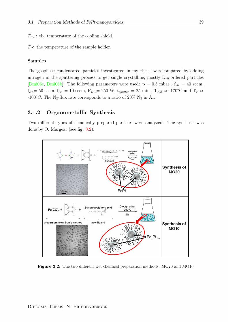
3.1.2 Organometallic Synthesis
Two different types of chemically prepared particles were analyzed. The synthesis was
done by O. Margeat (see fig. 3.2).
Figure 3.2: The two different wet chemical preparation methods: MO20 and MO10
Diploma Thesis, N. Friedenberger

40 Experimental Techniques
The first sample (MO20) was prepared by the simultaneous reduction of the two pre-
cursors iron bis-bistrimethylsilylamide (Fe[N(SiMe3)2]2) and platinum acetylacetonate
(Pt(acac)2). Hexadecylamine and oleic acid were used as ligands, and trimethylbenzene
(mesitylene) as solvent. The mixture was then heated at 200◦C during 48 hours under 3
bar of dihydrogen pressure (reducing agent).
The second sample (MO10) was prepared by a simultaneous decomposition and reduc-
tion of the two precursors iron pentacarbonyl (Fe(CO)5)and platinum acetylacetonate
(Pt(acac)2) according to Sun’s method [Sun00] and adding 2 − bromooctanoic acid as a
new ligand. The solvent was dioctyl ether. The solution was heated at 280◦C during one
hour and afterwards washed by adding ethanol and centrifugated.
Both samples used for the HRTEM investigations were common TEM copper grids covered
with an amorphous carbon layer on which a drop of the solution was dried. After drying
the grids were washed in aceton to remove dispensable ligands.
3.2 Microscopes
For my investigations I used two microscopes. The TecnaiF20 ST in Duisburg for the
pre-characterization of the samples and the (OAM), a modified Philips CM300FEG/UT,
at the National Center for Electron Microscopy in Berkeley for the focal series acquisitions
and the tomography studies. Both microscopes are shown in fig. 3.3. Technical details can
be found in the Appendix section (A-1).
3.3 Software
Reconstructing the Exit Wave (electron wave function) of the sample was done with the
TrueImage Professional software package by FEI. TrueImage consists of two independent
parts, one part is used for the acquisition of a focal series in the microscope. The other one is
for the reconstruction of the complete phase and amplitude information from a focal-series
of HR-images. The TrueImage algorithm is patented and uses linear approaches as well as
non-linear approaches. The advantage of this reconstruction consists in eliminating imaging
errors like the spherical aberration of the microscope. Also the delocalization effects caused
through the FEG (Field Emission Gun) source are removed so that the obtained images are
directly interpretable beyond the point-resolution. The professional version of TrueImage,
which was used for this thesis, also offers the features of manual correction of coma and
3-fold astigmatism and the automatic correction of 2-fold astigmatism and defocus [Fc06].
Layer resolved Lattice Relaxation in Magnetic FexPt1−x Nanoparticles

3.4 W-tip Preparation 41
Figure 3.3: Microscopes: a) CM300 - (NCEM, Berkeley, CA) b)Tecnai - (University Duisburg-Essen, Duisburg)
A description of how the method of Exit Wave Reconstruction works was given in Chapter
2.2.2 and a short manual of how to use this software is given in Appendix A-5.
3.4 W-tip Preparation
As described before one aspect of this thesis was the preparation of samples which can be
studied by HR-TEM for structural analysis and Field Ion Microscopy (FIM) for chemical
analysis. For FIM sharp tips with a radius of curvature < 100 nm are needed. Therefore
the idea was to prepare tips which can be studied in the TEM and afterwards being used
as a FIM-sample. This idea also included the design of a special TEM-holder allowing
the investigation of these tips. This holder is described in section 3.5. Typically used
FIM-tips are etched Ag- or W-wires which are compressed in a Cu-tube of 1.5 mm outer
and 0.5 mm inner diameter. The entire length of this sample is limited to 20 mm and not
less than 17 mm. The length of the Cu-tube should be between 10 mm and 15 mm. For
my investigations I chose Cu-tubes of 15 mm length and a W-wire because of the better
expected adhesion character for the FePt-nanoparticles. To center the wire as good as
possible in the Cu-tube both were centered in a lathe. The centering becomes important
Diploma Thesis, N. Friedenberger
42 Experimental Techniques
for tomography, since if it was not centered, a step-wise rotation around its axes would bring
the tip out of the focus. With a special flat-nose pliers the Cu-tube was compressed so that
the W-wire was fixed. Although the lathe was used for centering, this did not guarantee
having the wire centered afterwards but gave the best results comparing to other tried
methods. After centering and fixing the W-wire it was cut to a length of approximately 5
mm (up from the Cu-tube).
For the electro-chemical etching of the tips a special construction developed by D. Severin
in his diploma thesis was used [Sev03]. With this it was possible to dip the wire in a
controlled way into the electrolyte. 2 M NaOH was used as electrolyte. FIM-experts (T.
Al-Kassab, E. Marquis) told me to try alternate current, a voltage between 1 and 5 Volts
and a successive retracting out of the electrolyte to get sharp tips. To find the optimum
parameters more systematic experiments have to be done. After the etching process the
tips had to be washed several times in distilled water to remove the rest of the electrolyte.
After this, the tips were also dipped in methanol to remove all the water out of the Cu-tube.
Methanol evaporates quickly and takes the water with it.
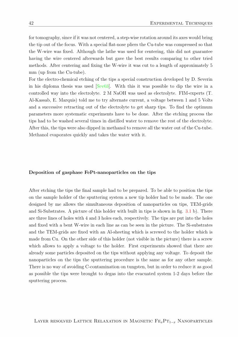
Deposition of gasphase FePt-nanoparticles on the tips
After etching the tips the final sample had to be prepared. To be able to position the tips
on the sample holder of the sputtering system a new tip holder had to be made. The one
designed by me allows the simultaneous deposition of nanoparticles on tips, TEM-grids
and Si-Substrates. A picture of this holder with built in tips is shown in fig. 3.1 b). There
are three lines of holes with 4 and 3 holes each, respectively. The tips are put into the holes
and fixed with a bent W-wire in each line as can be seen in the picture. The Si-substrates
and the TEM-grids are fixed with an Al-sheeting which is screwed to the holder which is
made from Cu. On the other side of this holder (not visible in the picture) there is a screw
which allows to apply a voltage to the holder. First experiments showed that there are
already some particles deposited on the tips without applying any voltage. To deposit the
nanoparticles on the tips the sputtering procedure is the same as for any other sample.
There is no way of avoiding C-contamination on tungsten, but in order to reduce it as good
as possible the tips were brought to degas into the evacuated system 1-2 days before the
sputtering process.
Layer resolved Lattice Relaxation in Magnetic FexPt1−x Nanoparticles

3.5 TEM-Holder for Tomography 43
Figure 3.4: New TEM-holder: a)full view b)tip extended - built-in situation c) tip retracted -position as in TEM
3.5 TEM-Holder for Tomography
The FIM-tips should be analysed in the TEM first before being used as a FIM-Sample.
Since the FIM-tips do not fit into a standard TEM-holder, a new one had to be constructed.
The idea was to be able to fully rotate around its axis and to mechanically protect the tip
during the transfer into the evacuated TEM-column. A ball bearing offers the opportunity
to insert a guiding rod on the top on which the tips can be fixed by simply pulling it with
tweezers into the suited vent. By rotating the gray sleeve at the end of the holder the bar
moves forwards and backwards and the tip can be retracted till it is fully screened by the
protection sleeve (see a) in figure 3.4). With this construction translation and rotation are
completely independent.
Diploma Thesis, N. Friedenberger


Chapter 4
Results and Discussion
In this chapter three different methods for the determination of the lattice parameter of
FePt nanoparticles with sub-angstrom resolution are compared and the results are dis-
cussed.
It is shown that all lead to the same result within the error bar. First Fourier and bright
field analysis for the lattice constant determination are shortly described and the error
estimation for both methods is described in section 4.1. The Quantitative HR-TEM (”Z-
contrast”) as possibility for columnwise chemical analysis is discussed in section 4.2. In
section 4.3 all results for the gasphase particles and in section 4.4 for the colloidal particles
are presented.
Another question, if small changes of the lattice constant, e.g. due to the L10-phase, can
be detected, is addressed in section 4.3.1. The difference between the lattice constant in
a- and the c-direction is 3.8% (table in section 6.2)[Lan92].
4.1 Software Analysis of TEM images
FFT analysis of bright field images
The lattice constant a and the lattice plane spacing dhkl of fcc structures are related acc.
to eq. 4.1. For the tetragonal distorted L10-structure this equation is more complicated
and given in Appendix: eq. 6.2.
a = dhkl ·√h2 + k2 + l2 (4.1)
The miller indices (h,k,l) can be determined by the Fast Fourier Transform (FFT)
of the bright field image or better the reconstructed phase image of the particle (4.1).
Diploma Thesis, N. Friedenberger

46 Results and Discussion
Figure 4.1: : Scheme of the FFT analysis steps as described in the text.
The FFT pattern corresponds to the diffraction pattern which can be recorded in another
TEM mode. The distance between one diffraction spot (h,k,l) and the center spot (0,0) is
the reciprocal dhkl-spacing. The distance between the two diagonal equivalent diffraction
spots was measured and then the reciprocal of half the distance was determined to get
the dhkl-values. In fig. 4.1 the whole procedure is demonstrated : First a squared frame
as large as possible (overlap with neighboring particles has to be avoided) for the FFT
has to be marked (b). The larger this frame can be chosen the finer is the resolved FFT
image(c). This FFT image was magnified so that the diffraction pattern was better visible
(not changing the total number of pixels)(d). The distance between two diffraction spots
is determined from an intensity profile (e). dhkl and the lattice constant a are calculated
according to eq. 4.1.
Layer resolved Lattice Relaxation in Magnetic FexPt1−x Nanoparticles

4.1 Software Analysis of TEM images 47
”Bright field” analysis
The layer resolved structure can be determined from intensity profiles (linescans) across
atomic columns, observed in bright field TEM images (fig. 4.2). The images were scaled
by 400% for easier analysis.
Assuming that the spacings are equal, the average d-spacing is calculated by dividing the
distance between the intensity maximum of the first and the last measured atomic column
by the number of atomic columns minus one. For non periodic structures the distance
between two adjacent columns is measured.
For the latter method the error is much larger than for the averaging method, since it is
directly given by the resolution, which I have limited to one pixel, and small changes in
the ”pixel” separation are not averaged out. For perfect periodic structures it is evident
that the larger the distance the smaller the error.
In this work mostly both analysis methods were performed. The FFT of a linescan (referred
to as FFT ls in table 4.3) was taken in to see if there is more than one peak, i.e. more than
one periodicity in the lattice spacing. This method, however, leads to no improvement
as the analysis for the series23 and for the series62 particle has shown. The uncertainty
for the FFT graphs was almost 5% and consequently too large for the needed accuracy
(for an example, see Appendix: A-4). Therefore it was not used for detailed relaxation
investigations.
Linescan parameters are the length and the width of the line in pixels (integration
width). If it is set larger than 1 the resolved linescan is an averaged intensity profile over
this width. It is always useful to slightly increase the integration width to make sure that
all maxima are included. If it is only set to one pixel also artifacts and noise contribute
strongly to the intensity profile. By increasing the integration width these effects are
weakened and the intensity profile is smoothed. Large integration widths, as used for
”fast” analysis can also result in artifacts as discussed in section 4.3.2.
Fig. 4.2 illustrates the effect of changing the width of a linescan. The two viewgraphs
show the same linescan as indicated in the image above for different integration widths
from 1-20 pixels. The framed area of the left viewgraph is magnified in the right one. Also
the mathematical average of those linescans was formed and it turned out that the 10 pixel
integration width was in good accordance to this average and consequentially was used for
further investigations of single layer linescans.
Diploma Thesis, N. Friedenberger

48 Results and Discussion
Figure 4.2: . This graph shows several intensity linescans for different integration width (i.w.)values. <i.w.> is the average over all linescans.
Evaluation of error bars
For the analysis methods presented in the two previous sections the accuracy and the
resolution is limited by the quality of the micrograph and the software. The analysis
in this thesis was done with the DigitalMicrograph(TM) 3.6.5 for GMS 1.1 software by
Chris Meyer, Doug Hauge and the Gatan Software Team. The resolution cannot be more
accurate than one pixel in the micrograph. Fig. 4.3 shows a linescan for the ”series 62”
Layer resolved Lattice Relaxation in Magnetic FexPt1−x Nanoparticles

4.1 Software Analysis of TEM images 49
colloidal particle1.
The measured peak separation (in [200]-direction) is 9.96 nm−1 in a). The circles mark the
areas in which the peak intensity is the same - that means an uncertainty in the positioning
of the distance determination tool. In b) the smallest resolvable interval is shown, which
is 0.2 nm−1 here. Hence, the start or end position of the linescan can only be varied by
this amount in one direction.
With eq. 4.2 the upper and the lower error limits of the distance x/2 can be determined.
We calculate 1/d200 = x/2 = 4.98 nm−1 for the reciprocal d200-spacing and 0.2008 nm for
the absolute d200-spacing (d200 = a/√
4).
dhkl =1
x2±∆
(4.2)
The error bar to the upper boundary is bigger than for the lower boundary, approxi-
mately 0.4%. Here it is 0.1931 nm < 0.2008 nm < 0.2092 nm (-3.8%, +4.2%). The error
bar depends on the size of the frame for the FFT but can be pushed below 2%. In the
example a small frame was chosen.
As already mentioned before, the error for the bright field intensity linescans is also the
pixel-uncertainty, for my investigations of the phase images typically 0.00505 nm. This
value is due to the scaling of 0.0202 nm/pixel of the phase images reconstructed from the
CM300 focal series and the rescaling by 400%. Even though this interrelationship between
the scaling and the error suggests that the larger the scaling the smaller the error it is clear
that larger scaling is physically useless. By increasing the number of pixels the informa-
tion content is not increased since it is limited to the number of pixels of the reconstructed
images. Magnifying the image only makes the positioning of the linescans easier. Apart
from that, the scaling of the bright field image does not effect the FFT image at all. A
magnification of 400% allowed an easier positioning of the cursor on the computer screen.
The previous error consideration for the FFT analysis is valid for every single diffraction
spot measurement, whereas the error bars in the following figures are given - if no other
specification is given - by the standard deviation of the average of distances determined in
different directions.
Other possibilities of investigating relaxations
For the layerwise investigation of the lattice parameter I used the ”linescan method” but
there exists another possibility: NCEM developed a software called ”Derip” for the deter-
1The Scherzer image was used for this case.
Diploma Thesis, N. Friedenberger

50 Results and Discussion
Figure 4.3: Limit of the FFT-analysis. a) Shows the linescan also shown in fig. 4.1. The redcircles indicate the peaks used for the distance estimation. b) Shows the minimum resolvableinterval ∆ by software which corresponds to one pixel in the micrograph.
mination of the intensity maxima in a picture. The maxima are evaluated by a software
algorithm that marks these positions with a so-called ”blob”. A schematic view and a
short description of a detection process with ”Derip” is given in fig. 4.4. These ”blobs”
can be recorded and exported as a .dat-file into an analysis-program like ORIGINTM .
”Derip” is said to work with an accuracy of 0.1 pixel. When the .dat-file is imported into
ORIGIN all y-values have to be multiplied by minus 1 to represent directly the positions
of the recorded blobs. In order to plot the blobs in the aspect ratio as taken from the
image the ratio of x/y-axis has to be adjusted, in the case of that particle shown in the
scheme it is 1.36 (750/550). A special tool for ORIGIN7.5 enables the measuring of the
distance between two points. This distance determination tool can be used by eye only.
Its accuracy is so rough that a direct investigation of the lattice relaxation was not done
with the Derip images.
Layer resolved Lattice Relaxation in Magnetic FexPt1−x Nanoparticles

4.1 Software Analysis of TEM images 51
Figure 4.4: Working procedure for Derip: First the image has to be scaled to 1024×1024 pixel2.Secondly the image is filtered exponentially and also with a Wiener filter to increase contrast anddecrease the noise signal from the amorphous part of the sample. Then the blobs detectionparameters are optimized till all or as many atom columns (intensity maxima) as possible aredetected. Fourth a frame can be set to choose the area of blobs which are to be recorded. Theblobs in this area are automatically put into a .dat-file yielding the corresponding coordinates.
Discussion of results
The discussions following in the next sections will include the analysis of average values
by less than 1%. In terms of the absolute error bar these discussions have to be regarded
very critically. Nevertheless they were performed to emphasize small changes between
different analysis methods and possibly see some tendencies in the variation of the lattice
parameter. The maximum precision obtainable from the EWR at the OAM is 2 pm [Xu05],
i.e. approximately 0.5% with respect to the bulk but up to 1.5% (d222) for the smaller d-
spacing values for FexPt1−x.
Diploma Thesis, N. Friedenberger

52 Results and Discussion
4.2 Quantitative HR-TEM
In this section I discuss a simplified model for quantitative HR-TEM analysis as a possible
tool to identify the elemental composition in atomic columns. As described in section
2.2.1 this contrast provides chemical sensitivity for single atomic columns. The exit wave
reconstructed phase images represent the real lattice structure, i.e. the positions of atomic
columns. The intensity in those images corresponds to the phase of the electron wave after
scattering of the potentials in the atomic column.
The task is to identify the chemical composition of the single columns from intensity (phase)
profiles across atomic columns. The following simple analysis is approximately valid for a
total phase shift smaller than 2π (see chapter 2.2.1, extinction distance). This limits the
analysis to real samples with a thickness of less than 5 nm for large Z-elements like Pt (Z
= 78) or Au (Z = 79) or less than 40 nm for light elements like C (Z = 6)(fig. 2.5).
To illustrate the possible information which could be obtained one chemically disordered
(fig.4.5) and one L10-ordered (fig. 4.6) 10-shell cuboctahedron were modeled. Both are
viewed from the [011]-direction. The electron beam is assumed to come from top and
scatters along the atomic columns. Pt-atoms are light blue and Fe-atoms dark grey. The
L10-cuboctahedron has top and bottom Pt-surface layers. In figure 4.7 the simple Z-
dependence of the signal which is proportional to Z1.7 for STEM and to Z2/3 for HR-TEM
are plotted for columns 1-17 of the model. The column signal was calculated according to
equation 4.3 and is also given in table 4.1.
Intensity = x ∗ 26y + (n− x) ∗ 78y (4.3)
n is the total number of atoms in the column, x is the number of Fe-atoms in the column
and y is 1.7 for the STEM and 0.67 for the TEM calculation. 26 is the atomic number
Z for iron and 78 is Z for platinum. Figure 4.7 is an estimate of the expectable signal
if dynamic scattering would be removed. Only the Z-dependence was calculated and any
other influences or offsets neglected. The number of Fe-atoms in each column is marked
with a green striped bar.
The even-numbered columns in the L10-phase consist of Fe-atoms, the odd ones of
Pt-atoms only. For the chemically disordered particle the distribution is 50:50 for even-
numbered columns whereas for odd-numbered columns there is one more Fe-atom than
Pt-atoms. There are three exceptions: column 1 which consists of one single Pt-atom
as for the L10-phase and column number 11 and 15 which have one more Pt-atom than
Fe-atoms which results in a signal increase by 14% for the STEM and 6.5% for the HR-
TEM. Such a small difference when replacing Fe and Pt can only be detected by STEM if
Layer resolved Lattice Relaxation in Magnetic FexPt1−x Nanoparticles
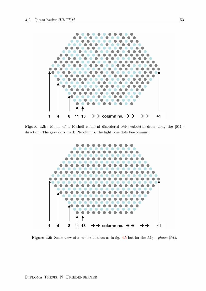
4.2 Quantitative HR-TEM 53
Figure 4.5: Model of a 10-shell chemical disordered FePt-cuboctahedron along the [011]-direction. The gray dots mark Pt-columns, the light blue dots Fe-columns.
Figure 4.6: Same view of a cuboctahedron as in fig. 4.5 but for the L10 − phase (fct).
Diploma Thesis, N. Friedenberger

54 Results and Discussion
1 2 3 4 5 6 7 8
1 0 0 1 1646.49655 1646.49655 18.25561 18.25561
2 1 2 2 508.72688 1900.85999 17.55277 27.032
3 1 0 3 4939.48964 3547.35654 54.76684 45.28761
4 2 4 4 1017.45376 3801.71998 35.10553 54.06399
5 2 0 5 8232.48274 5448.21653 91.27806 72.3196
6 3 6 6 1526.18065 5702.57997 52.6583 81.09599
7 4 0 7 11525.47584 5956.94341 127.78929 89.87237
8 4 8 8 2034.90753 7603.43996 70.21106 108.12798
9 5 0 9 14818.46893 7857.8034 164.30051 116.90436
10 5 10 10 2543.63441 9504.29995 87.76383 135.15998
11 5 0 11 18111.46203 11150.79649 200.81173 153.41559
12 5 10 10 2543.63441 9504.29995 87.76383 135.15998
13 6 0 11 18111.46203 9758.66339 200.81173 143.93636
14 5 10 10 2543.63441 9504.29995 87.76383 135.15998
15 5 0 11 18111.46203 11150.79649 200.81173 153.41559
16 5 10 10 2543.63441 9504.29995 87.76383 135.15998
Table 4.1: Theoretical Z-contrast of the cuboctahedra shown in fig. 4.5 and in fig. 4.6. In thistable column 1 is the index, column 2 the number of Fe atoms in the respective columns for thechemical disordered model, column 3 the number of Fe atoms for the L10-ordered case, column4 the total number of atoms in the column, columns 5 and 6 the STEM signal for the chemicaldisordered and the L10-ordered case and columns 7 and 8 the HR-TEM signal for the chemicaldisordered and the L10-ordered case, respectively.
Layer resolved Lattice Relaxation in Magnetic FexPt1−x Nanoparticles

4.2 Quantitative HR-TEM 55
Figure 4.7: Calculated Z-contrast for the two cuboctahedra shown in figures 4.6 and 4.5. Theintensity values are divided by the factor 1000 with respect to those given in table 4.1. The uppergraph shows the intensity STEM Z-dependence and the graph below the intensity for the HR-TEM Z-dependence. Note the different intensity scales! The green lined bar in each viewgraphgives the number of atoms in the corresponding column. The green striped column gives thenumber of Fe-atoms in the chemically disordered column accordingly. For the L10-phase the evencolumn numbers consist only of Pt-atoms and the odd ones only of Fe-atoms, see fig. 4.6.
Diploma Thesis, N. Friedenberger

56 Results and Discussion
the signal/noise-ratio improves (2.4). The HR-TEM simulation of the Z-contrast will be
discussed in more detail. Comparing columns 1 and 2 it is evident that the signal is the
same for one Pt-atom per column or for two Fe-atoms per column (fig. 4.7 bottom, red
bars). That means, it is impossible to distinguish in-between the two cases. By further
considerations it also becomes obvious that there is no constant ratio which would indicate
for one more Pt- or Fe-atom in a column. It depends on the number of atoms per column
very sensitively. One should note that also columns which are not next to each other may
give similar signals depending on the Pt/Fe composition in the column. Column 7 for the
L10-phase and column 10 for the disordered phase give an almost identical signal, although
the number of atoms differs by three.
Hence the determination of column compositions from a single image of a particle is im-
possible in the center of a particle. A flat intensity profile could have two reasons:
1. the number of atoms per column and the composition of all columns is the same. In
my simplified model it would make no difference where the Pt and Fe are positioned
in the column. In a refined more realistic model the actual positions of the different
elements will influence the overall column Z-contrast.
or
2. the chemical composition changes from the inner to the outer columns - more atoms
of larger Z are in the outer columns which usually consist of less atoms.
That means, to be able to make any statement about the chemical compositions of the
atom columns the shape of the particle has to be known since a normal TEM image is only
a 2-dimensional projection. Shape information can be obtained from tomography investi-
gations [Bal06], that is from high resolution images taken along different crystallographic
axes of the nanoparticle.
Image acquisition of the same particle in different orientations can take a long time
and beam damage to the sample is likely. First tomography experiments on FePt-cubes
at the NCEM in Berkeley also showed that there is significant change in the form of
the particles for only a few tilt-steps [Sud06]. Therefore it is necessary to control beam
damage. This can be achieved by the application of low-dosed techniques or by the choice of
appropriate voltages. The challenge for the future is to acquire such tomography series, that
is along many directions focal series have to be recorded without damaging the particles.
Even if this can be achieved, the challenge remains to identify the number of atoms per
column viewed from different directions. Due to the ”phase wrapping” of the exit wave
the particles must be small enough in all these directions. The model of the nanoparticle
Layer resolved Lattice Relaxation in Magnetic FexPt1−x Nanoparticles

4.2 Quantitative HR-TEM 57
Figure 4.8: . Scheme of a 10-shell perfect cuboctahedron along the [001]-, [011]- and the[111]-direction.
according to the tomography results would undergo a simulation process with a HR-TEM
simulation software for the zone-axis the focal series were taken from. The phase images
reconstructed from those series have to be compared to the corresponding simulated phase
images. In the framework of this thesis it was not possible to recover the structure and
its chemical constituents yet. In order to understand and interpret the recorded images
I compared image simulations with the experimental data. However, this is possible only
within limitations because the image contrast in experimental images is commonly smaller
than in the simulations (Stobbs factor) and phase-wrapping has to be considered [Kis06b].
First simulation results
To simulate the TEM phase contrast from real space models of different crystals with
different compositions the MacTempasX software by R. Kilaas [Kilb] was available at
NCEM, LBL. This program was not optimized for small particle simulation. The x,y,z
coordinates for a cuboctahedron had to be defined in a data file which could be read by
the software.
For simplification I start the discussion for a pure Fe-cuboctahedron. The beam is in
the [001]-direction so the [001]-layer of the particle is seen. Due to the geometry of the
cuboctahedron this layer appears as a square. The resulting phase image is shown in fig.
4.10 on the left. In the right image the central Fe-atom was replaced by a Pt-atom. The
gray scale phase images show no significant difference at the center column. The plot-
ted intensity profiles, however, for the linescans show a phase shift of approximately 0.3
rad, which is equal to 12%. That means the Pt-atom gives a 12% larger signal than the
Diploma Thesis, N. Friedenberger

58 Results and Discussion
Figure 4.9: . Cross section views of the cuboctahedron used for the simulations. a) surfacelayer - used for linescan edge b) center layer - used for linescan middle
Fe-atom. The difference between the other columns for which the number of Fe-atoms is
alternating between 10 and 11 (see also fig.4.9b)) is only 0.05 rad (2%). The same lines-
cans were also done for the amplitude images (modulus) of the exit wave (fig.4.11). In this
figure the difference is much smaller, 4% only if the central Fe atom is replaced by Pt. In
the amplitude (modulus) signal, on the other hand, the different number of Fe atoms in
the columns can be resolved easily. As expected the signal for the outermost columns is
larger than for columns consisting of the same number of Fe-atoms in the inner part of the
particle because of the dynamical scattering. For the columns consisting of 11 Fe-atoms
also next to the center column with the Pt-impurity the modulus is even smaller.
In analogy to this observation, there are also differences in the phase image for the outer-
most columns. Here the phase is smaller than for any other 11 Fe-atom column and even
smaller than for a 10 Fe-atom column. It makes clear that the phase signal of the recon-
structed image is not easy to understand and that simulations for many specific models
are mandatory.
A linescan (fig. 4.12) along a surface layer of the cuboctahedron was also looked at in
detail. Fig. 4.9a shows this surface layer, the electron beam direction is from top to the
bottom. For the columns consisting of 1-10 Fe-atoms the slope of the phase shift is almost
constant, but for the center column, the signal is smaller than expected, also with respect
to the value of 2.5 rad of the middle linescan. It would be interesting to see if the slope
is the same as it is for the other ones if there would be two columns more, i.e. one center
Layer resolved Lattice Relaxation in Magnetic FexPt1−x Nanoparticles

4.2 Quantitative HR-TEM 59
Figure 4.10: Simulated phase images for a 10-shell Fe cuboctahedron and phase versus pixelplot of the two middle linescans. The images show the [001]-direction. In the particle on theright the center Fe-atom was replaced by an Pt-atom.
column consisting of 12 and another next to it with 11 Fe-atoms - so that the distribution
is symmetric. Then it would be clear if maybe 11 Fe-atoms in a column is a critical size
or if it is really an effect based on the surface geometry.
It turns out to be possible to count atoms in the 1-10 Fe atom columns from the magnitude
of the phase signal, which has an almost constant phase shift of 0.2rad per atom (9% phase
shift from the 9- to 10-atom column). This is a huge difference compared to the shift for
the center linescan. There the shift between the 10- to the 11-atom column is 0.05rad, i.e.
Diploma Thesis, N. Friedenberger

60 Results and Discussion
2%. This is a perfect example for dynamical scattering and why it has to be considered.
Although this last figure suggests that it might be simple to distinguish between different
atom numbers in atom columns, there is also another point to mention, the position of the
atom columns with respect to the substrate: It will certainly make a difference if there is
space between the last atom of the column and the substrate or if the column is touching.
This effect was not considered in my simulations.
Summary
In this section it is demonstrated that quantitative HR-TEM could be used for the de-
termination of the chemical composition of atom columns if the shape of the particle is
known. It is shown that due to the effects of dynamical scattering different signals can
be observed even when the column composition is identical but the column is located at
different positions. Ambiguity of the signal for a specific number of atoms in a column
with different compositions is also discussed.
Figure 4.11: Modulus of the middle linescans as shown in fig. 4.10.
Layer resolved Lattice Relaxation in Magnetic FexPt1−x Nanoparticles

4.2 Quantitative HR-TEM 61
Figure 4.12: Phase signal of a 10-shell hollow particle (central shells 0-5 missing). The edgelinescan is equal to the one of a full cuboctahedron. The position of the edge linescan is alsoshown in fig. 4.10.
All these aspects lead to the conclusion that detailed simulations have to be done in order
to verify the phase signal. To simplify the simulation process the chemical composition
of the particle should be known. From my results I can conclude that the determination
of elemental composition from HR-TEM (EWR) phase and amplitude images will be suc-
cessful only with modeling and simulations.
Diploma Thesis, N. Friedenberger

62 Results and Discussion
4.3 Cuboctahedra
The samples were prepared as described in section 3.1.1. The nitrogenized particles [Dmi03]
are expected to be mostly single crystalline and L10-ordered (fig. 6.1). Of the approxi-
mately 100 nanoparticles imaged, most were orientated in the typical [011]-zone axis or
slightly tilted. Only very few were found in the [001]-zone axis and one was observed lying
in the [111]-direction. These statements are valid for the Scherzer images taken before the
focal series acquisition.
According to [Dmi06a] the EDX analysis yields a composition of 50% Fe and 50% Pt ± 5
at%. The TEM overview image and the associated size distribution are shown in fig. 4.13.
The LogNormal fit y = y0 + A/(sqrt(2*p)*w*x)*exp(-(ln(x/xc))2/(2*w2)) yielded y0 =
2.21886 ± 0.78581, xc = 5.73156 ± 0.03166, w = 0.06994 ± 0.00593 and A = 35.55568 ±2.48644. A mean diameter of 5.73 nm± 5.5% was obtained.
Figure 4.13: TEM overview image of the gasphase prepared sample (magnification: 63k) andassociated size distribution.
Layer resolved Lattice Relaxation in Magnetic FexPt1−x Nanoparticles
4.3 Cuboctahedra 63
4.3.1 Lattice structure
In this section the mean lattice parameter for an ensemble of EWR particles was determined
by FFT analysis and compared to the bulk value. Furthermore the mean lattice parameter
of one single well-oriented (L10-ordered) particle (series23) is investigated by the three
different methods described in section 4.1. In addition a direction dependent analysis of
the lattice parameters a and c was performed. Furthermore the lattice relaxation for this
particle was investigated.
As expected [Sta03c, Dmi03] the lattice structure of the gasphase synthesized particles was
observed to be either fcc or fct.
Mean lattice parameter a of several gasphase prepared NPs
To determine the mean lattice parameter a the EWR images were FFT analyzed. The
particles were not stable enough on their zone axis, therefore a direction dependent analysis
could not be done and the average over all directions <aFFT> = 0.397 nm ± 0.9% was
determined. These results are also shown in fig. 4.14, with the standard deviation of all
measured directions for one series as the error bar. With respect to the FePt bulk value of
0.381 nm the mean value of those series is enlarged by 4.1%.
In more detail, the mean lattice parameter for the six focal series (04, 15*, 16/16*(same
focal series, different particles), 17*,19, 21) varies between 0.391 nm < <aFFT> = 0.397
nm < 0.401 nm. With respect to the bulk lattice parameter this is an enlargement interval
from +2.6% to +5.2%. In conclusion every single analyzed particle showed an lattice
expansion out of the error bar with respect to the FePt bulk value. The question is if this
is a real enlargement or only an artifact due to tilting of the particle.
The influence of tilt to the lattice constant was simulated by J.-O. Malm and M.A. O’Keefe
[Mal97]. It was shown that images tilted by 15◦ yield a mean deviation of more than 1% for
the lattice spacing measurement. The minimum and maximum values of single directions
showed also deviations up to 10%. They concluded that the power spectrum is a good tool
to determine average lattice constants. If the {111} and {200} diffraction spots (see for
example fig. 4.16 b)) are not at the correct positions when imaging along the [110]-direction,
simulations assuming different structural models to obtain the real crystal structure are
required.
The reflection positions and angles between the directions were approximately evaluated
to make sure that the structural data of the FFT analysis are related to the real lattice
spacings. Consequently only particles with an ”almost perfect” power spectrum (FFT
pattern), like the ”series23” and the ”series62” particle, were further investigated to look
Diploma Thesis, N. Friedenberger

64 Results and Discussion
Figure 4.14: Mean lattice parameter <aFFT > (FFT analysis) of different particles on the samesubstrate - series18 excepted (Scherzer image). The (green) box marks one particle, which wasmeasured in three successive focal series.
for surface-layer relaxations. Therefore small tilting effects are already included in the
error bar and the 4.1% expansion of the mean lattice parameter is a real expansion.
Is an expansion of that order specific for nanoparticles because of the smaller surface
energy with respect to the bulk or because of the presence of oxygen as discussed for
colloidal particles [Tro04], or is it due to the analysis and image acquisition method? If the
third point proves true, the next question arises: Is this enlargement effect time dependent,
i.e. the longer the particles are investigated under the beam, the larger is the measured
lattice constant?
Time dependence of lattice expansion?
The lattice parameters in fig. 4.14 were analyzed from focal series taken at the same day.
For series15* to series17* the same area was illuminated and the same sample could be
investigated. Obviously, for that particle, the lattice constant increases from series to series
by 1.3%, a hint that expansion might be a function of time. To be able to see a possible
Layer resolved Lattice Relaxation in Magnetic FexPt1−x Nanoparticles

4.3 Cuboctahedra 65
time dependence of the lattice constant the mean lattice parameters obtained by FFT
analysis (fig. 4.14) were put in chronological order and linearly fitted, see fig. 4.15. Ne-
glecting that series16 and series16* are different particles recorded in the same focal series
the slope is 0.00106nm/series, which would be equivalent to a series dependent increase
smaller than 0.3% in the lattice constant. Thus it is smaller than the measured 1.3% of
the series15*-series17*. Another point to mention is, that not all series were taken at the
same sample position, so the time of beam radiation on the respective sample area is un-
known. And although this linear fit has a positive slope, there are successive series where
the mean lattice constant decreases with respect to the previous acquired focal series, e.g.
series18 to series19. One may conclude that there is no prove for a time dependence of the
lattice parameter expansion. This was only assumed for the series15*-series17* nanopar-
ticle, whereas this apparent expansion lies completely within the error bar. Therefore, I
conclude that no time dependence of the lattice expansion can be extracted by these data
and other explanations as the presence of oxygen have to be considered. Experiments on
the possible time dependence of the lattice parameter expansion require that the particle
is stable on one zone-axis. The particle should also not lie to close to neighbor particles,
so that sintering (see fig. 6.7 in Appendix: Sintering) is avoided [Tro04].
Direction dependent analysis of the mean lattice parameter
The mean lattice parameter of the well orientated series23 fct particle, see fig. 4.16 is
direction-dependently investigated by three methods in this section.
In the FFT-image the superstructure additional diffraction spots are clearly visible. The
angles 54.74◦ ± 0.8% and 35.26◦ ± 0.8% which are the same for fcc- and fct-structures
were measured. This particle is very well oriented in the [011]-zone axis. Table 4.2 shows
the lattice constant and the dhkl-spacing obtained from the FFT analysis. The error is
given by the one-pixel uncertainty. It is maximal 3.8% for the {100}-direction. Within
the error range all directions give the same lattice parameter, the mean value of all direc-
tions is 0.3864 nm ±1.2%. This value is enhanced by 2.2% with respect to the fcc FePt
bulk value. Taking into account that this is a fct-structure, two different values of the
lattice parameter have to be determined. In table 6.2 (Appendix) the values are listed for
c/a = 0.96. For this c/a-ratio the reference value [Lan92] for a is 0.385 nm and 0.371 nm
for c, the [100]-direction, respectively. This consideration results in two new mean values,
0.3817 nm ± 2% for the c-direction, 0.3887 nm ± 1% for the other directions and c/a =
0.98 ± 3%.
Diploma Thesis, N. Friedenberger
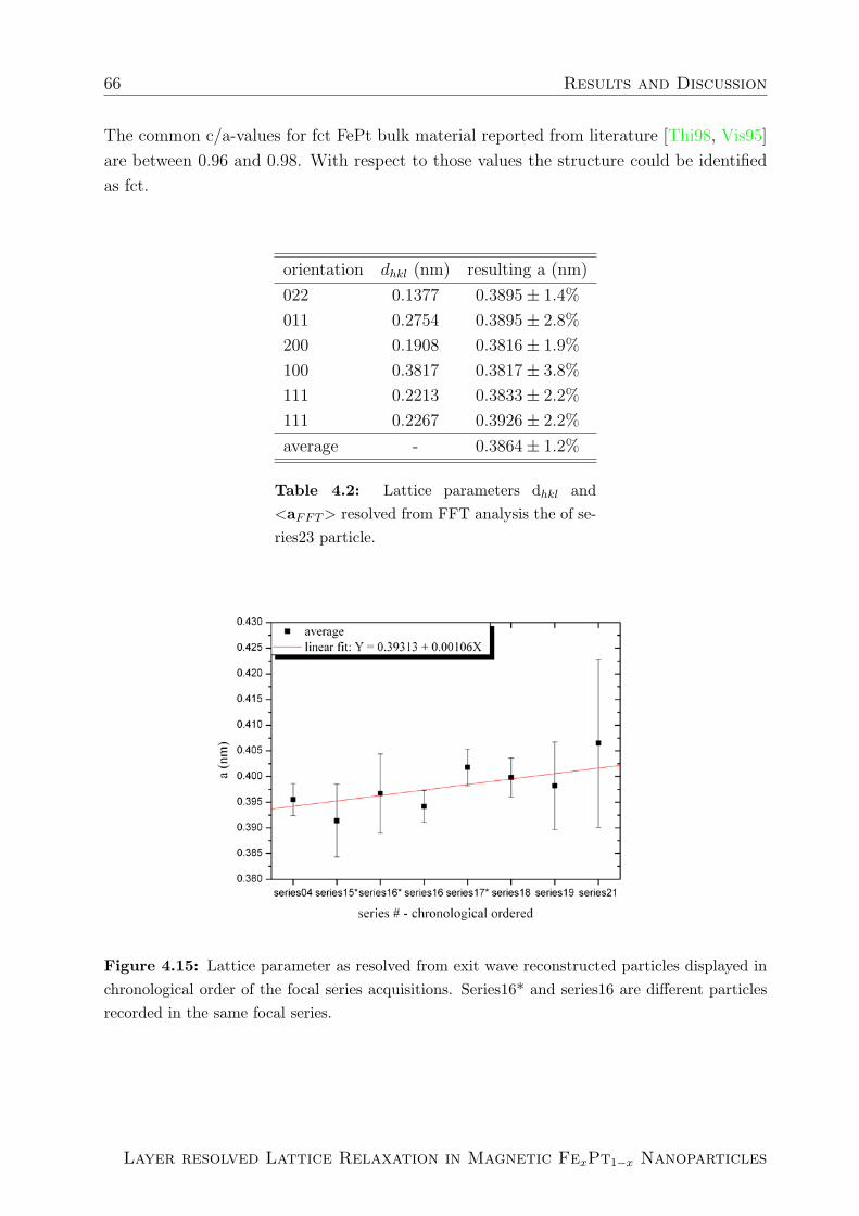
66 Results and Discussion
The common c/a-values for fct FePt bulk material reported from literature [Thi98, Vis95]
are between 0.96 and 0.98. With respect to those values the structure could be identified
as fct.
orientation dhkl (nm) resulting a (nm)
022 0.1377 0.3895± 1.4%
011 0.2754 0.3895± 2.8%
200 0.1908 0.3816± 1.9%
100 0.3817 0.3817± 3.8%
111 0.2213 0.3833± 2.2%
111 0.2267 0.3926± 2.2%
average - 0.3864± 1.2%
Table 4.2: Lattice parameters dhkl and<aFFT > resolved from FFT analysis the of se-ries23 particle.
Figure 4.15: Lattice parameter as resolved from exit wave reconstructed particles displayed inchronological order of the focal series acquisitions. Series16* and series16 are different particlesrecorded in the same focal series.
Layer resolved Lattice Relaxation in Magnetic FexPt1−x Nanoparticles

4.3 Cuboctahedra 67
Figure 4.16: a) Exit wave reconstructed phase image of one L10-ordered gasphase particle in[011]-direction. The linescan directions are indicated by (yellow) lines and arrows, the (whites)arrows hint at missing atom columns on the edges. b) FFT of the series23 phase image - the fctsuperstructure reflections are clearly visible (comp. to fig. 6.6 b) in Appendix).
direction dhkl (nm) a (nm) d(FFT ls) aFFT (nm)
100 0.1918 0.3836 0.1915 0.3830
110 0.1379 0.3900 0.1398 0.3954
111a 0.2233 0.3868 0.2248 0.3894
111b 0.2282 0.3953 0.2248 0.3894
all directions - 0.3889 nm± 1.3% - 0.3893 nm± 1.3%
Table 4.3: Averaged linescan (ls) analysis data of the series24 L10-ordered particleand average lattice parameter yielded from the FFT of the linescans.
The lattice parameter was not only investigated with this FFT method but also by
analyzing linescans in four directions of the phase image (fig. 4.17). Additionally, those
linescans were also Fourier transformed. This kind of FFT was done in order to look for re-
laxation phenomena, which would give more peaks in the spectrum for the relevant spatial
frequency interval. As already described in section 4.1 the accuracy in the FFT was not
good enough, so that only one frequency - the reciprocal of the averaged lattice spacing -
for a whole linescan - was resolved. The results from the linescan and the corresponding
FFT are given in table 4.3. For the linescans after 400% magnification of the image the
Diploma Thesis, N. Friedenberger

68 Results and Discussion
Figure 4.17: Viewgraph of the linescans taken in the four directions as indicated in fig.4.16 a).The apparent shift of the Fe sublattice will be shown to be an artefact of the analysis in section4.3.2.
integration width was chosen as 300 pixel (for a quick investigation) in all directions.
The measured spacings in [100]-direction are the spacings between the <200>-layers and
the ones in the [110]-direction between the <220>-layers, respectively. The error bar was
estimated by comparing two linescans along the same columns. The averaged deviation
between those two scans was taken as the error bar, since this error was slightly larger than
the value corresponding to one pixel. The error is relevant for the layer-to-layer measure-
ments (next section), see fig. 4.18 but not for the lattice parameter given by the average
spacings obtained from all linescan intervals. These measurements averaged over all direc-
tions (fig. 4.3) give a mean lattice constant <als> = 0.3889 nm ± 1.3% and <aFFT ls> =
0.3893 nm ± 1.3%, so it is identical to a = 0.389 nm within the error and enhanced by
0.6% with respect to the mean value from the FFT analysis of the bright field image.
Layer resolved Lattice Relaxation in Magnetic FexPt1−x Nanoparticles

4.3 Cuboctahedra 69
Also, this analysis of the [100]-direction yields smaller lattice parameters. Distinguish-
ing the a- and c-direction I find the mean values of <c> = 0.3833 nm and <a> = 0.3921
nm ± 1.5%. The average of the 110, 111a and 111b values in columns dhkl and dFFT differ
by 0.7%. <a> = 0.3921 nm is in the error bar with respect to <aFFT>= 0.3887 nm ± 1%
from the FFT image analysis. These values are identical. An averaging of the results of
all three analyzing methods gives: <a> = 0.391 nm, <c>=0.383 nm and c/a = 0.98 for
the particle of fig. 4.16.
4.3.2 Surface Layer Relaxation
The series23 particle was investigated in detail to identify a possible surface layer relaxation.
For a quick investigation of the surface layer relaxation the same linescans of 300 pixel width
as already used for the averaging part were analyzed maximum by maximum. The resulting
relaxation is shown in fig. 4.18 and the respective investigated layers are marked in the
linescan overview image, see fig. 4.17. Mind that in those two figures a), b) and c) do not
stand for the same directions. Along the [100]-direction (fig. 4.18 )a compression behavior
for the outermost layers of up to -5% is observed. The mean value 0.192 nm is increased by
3.5% with respect to the FePt bulk value for the fct-phase 0.1855 nm. Similarly to spacings
along other directions large variations are also observed in the core. An expansion up to
+8% compared to the mean value is found (This layer interval of 0.2075 nm d-spacing is
increased by 11.8% with respect to the Pt-bulk value). An unphysically large oscillation
of the d-spacing is observed in the [110]-direction. The oscillation varies between ±24% of
the mean value which definitely indicates an artifact in the analysis. The reason for this
apparently erroneous analysis is discussed below (p. 75).
The mean lattice spacing 0.1379 nm is enhanced by 1.3% compared to FePt in the fct
phase and by 0.8% compared to FePt3. The largest spacing values are found in the middle
part of the particle whereas the outermost layers are compressed up to 7% with respect to
the mean value.
As described before, the linescans along d200 and d220 do not show a relaxation. Linescan
111a reveals an expansion of the top two layers by 6.5% and a suppression of a similar
size on the opposite surface. The mean value 0.223 nm corresponds best to the FePt3 bulk
value of 0.2234 nm. From the L10-structure one would expect the value 0.2195 nm for
FePt so the measured mean lattice parameter would be enlarged by 1.8% and the largest
spacings by 8.2%. In this direction there was no relaxation tendency to recognize, since
there were both compression and extension found for the outermost layers and those values
Diploma Thesis, N. Friedenberger

70 Results and Discussion
Figure 4.18: Layer resolved analysis of the four linescans as indicated in fig.4.16a). Here a)shows d220 spacing, b) d200 spacing, c) d111a spacing and d) d111b spacing. Hereby the indices aand b in the d111spacing indicate the linescan.
were also found in the core.
The 111b-direction, see fig. 4.18 d), shows surface layer relaxation. The data for the
111b-linescan can also be found in table 4.5 and additionally the ratio of the first four
layer intervals for the outermost 5 layers can be found in table 4.6. For gasphase prepared
icosahedra a 9.4% outward relaxation of the surface layer compared to the inner layers was
measured in 111-direction [Wan06]. In case of the series23 particle an outward relaxation
of 6.3% compared to the mean value was measured at one surface (layer interval 1-2).
With respect to d111 = 0.2223 nm which was a typical value for the inner layers this gives
a 9.1% outward relaxation - almost the identical value as measured for the icosahedra
[Wan06].
The inner layers of this truncated cuboctahedron are mostly slightly extended by 1% with
respect to the bulk values (FePt: dfcc111=0.2200 nm, dfct
111 = 0.2195 nm (c/a = 0.96)) whereas
Layer resolved Lattice Relaxation in Magnetic FexPt1−x Nanoparticles

4.3 Cuboctahedra 71
this extension is 10.2% for the surface layer. To understand the large variations of the
lattice plane spacings one has to consider that the composition in the nanoparticle may
not be uniform. There are planes with pure Pt, pure Fe, or mixed composition. Conse-
quently, the spacings will vary due to the different atomic radii of Fe and Pt. In figure
4.19 and table 4.7 different compositions of two successive < 111 >-layers are assumed and
the resulting spacings for different crystal planes are listed. For the FePt-Pt layer spacing
the lattice parameter for FePt3 was used, the one of FePtfcc for the pure Fe-pure Pt layer
interval and FePtfct for FePt-FePt accordingly. Fig. 4.16 a) - following the 111b linescan
direction - illustrates that the last two measured layers only consist of few atom columns,
layer 25 presumably only of one. There are also missing edge atom columns indicated by
arrows.
The comparison of the two outermost layer-intervals of the 111b-linescan to bulk d-spacings
(table 4.4) shows that even assuming pure Pt-layers at the surface the surface spacing is
enlarged at least by 6.9%. Only interval 2-3 is in very good accordance with the Pt-bulk
value.
In case of the icosahedra a Pt-surface segregation model was developed to explain the ob-
served relaxation. In conclusion, for the cuboctahedron also surface segregation of Pt may
be the origin of the large outward relaxation found in the 111b-direction.
layer interval 1-2 2-3 23-24 24-25
d111 − spacing (nm) 0.242 0.2273 0.2475 0.2627
d111/Fe ∗ 100% 46.6 37.7 49.9 59.1
d111/Pt ∗ 100% 6.9 0.4 9.4 16.1
d111/FePt3 ∗ 100% 8.3 1.7 10.8 17.6
d111/FePtfcc ∗ 100% 10.0 3.3 12.5 19.4
d111/FePtfct ∗ 100% 10.2 3.6 12.8 19.7
Table 4.4: Percentage expansion of the outermost d111-layerintervals of particle in fig. 4.16 with respect to d111 spacingsfor different FexPt1−x layers (fig. 4.7).
Diploma Thesis, N. Friedenberger

72 Results and Discussion
In summary in section 4.3.1 it was shown that this L10-ordered truncated cuboctahe-
dron has a lattice constant increased by 1.5% for the a-direction (afct = 0.385nm) and by
3.5% for the c-direction (cfct = 0.371nm), respectively. The overall expansion of the lattice
plane spacing in the a and c direction cannot be attributed to a ”large surface relaxation” -
which was not observed. My analysis rather indicates an oscillatory behavior of the lattice
parameter within the particle with an enhanced average value. The <111>-surface planes
showed an outward relaxation whereas all other directions showed an inward relaxation
with respect to the mean as well as to the bulk value.
The observed surface compression of layers may be explained in terms of calculated results
of the surface relaxation and electronic structure of Zr(0001)[Yam94]. There an increase
in the local density of states for the surface atoms at the Fermi level relative to the bulk
atoms was observed. This increase is found to be closely related to the existence of surface
states and resonances around the Fermi level. It was shown that the unreconstructed hcp
structure of a clean Zr(0001) surface with more than 4% surface layer contraction is the
energetically most favorable structure. Accordingly this could be an explanation for the
observed contractions of the outermost layers of the nanoparticle and would support the
argument that surface tension exerts a compressive stress on nanoparticles. Thus the origin
of the outward surface layer relaxation - if it really exists - of the <111>-planes remains
an unsolved problem.
Layer resolved Lattice Relaxation in Magnetic FexPt1−x Nanoparticles

4.3 Cuboctahedra 73
layer interval dhkl (nm) variation from mean value (%)
1-2 0.2425 6.3
2-3 0.2273 -0.4
3-4 0.2071 -9.2
4-5 0.2273 -0.4
5-6 0.2223 -2.6
6-7 0.2223 -2.6
7-8 0.2223 -2.6
8-9 0.2324 1.8
9-10 0.2224 -2.5
10-11 0.2324 1.8
11-12 0.2324 1.8
12-13 0.2071 -9.2
13-14 0.2324 1.8
14-15 0.2324 1.8
15-16 0.2273 -0.4
16-17 0.2223 -2.6
17-18 0.2223 -2.6
18-19 0.2273 -0.4
19-20 0.2223 -2.6
20-21 0.2223 -2.6
21-22 0.2273 -0.4
22-23 0.2324 1.8
23-24 0.2475 8.5
24-25 0.2627 15.1
Table 4.5: Data for the 111b-linescan.
(1-2)-(2-3) (2-3)-(3-4) (3-4)-(4-5) (24-25)-(23-24) (23-24)-(22-23) (21-22)-(22-23)
6.7% 9.8% -8.9% 6.1% 6.5% 2.2%
Table 4.6: Relative d-spacings for 111b-linescan.
Diploma Thesis, N. Friedenberger
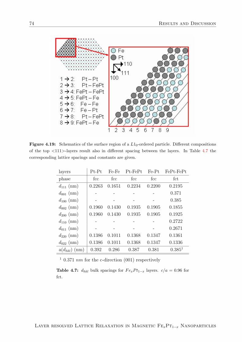
74 Results and Discussion
Figure 4.19: Schematics of the surface region of a L10-ordered particle. Different compositionsof the top <111>-layers result also in different spacing between the layers. In Table 4.7 thecorresponding lattice spacings and constants are given.
layers Pt-Pt Fe-Fe Pt-FePt Fe-Pt FePt-FePt
phase fcc fcc fcc fcc fct
d111 (nm) 0.2263 0.1651 0.2234 0.2200 0.2195
d001 (nm) - - - - 0.371
d100 (nm) - - - - 0.385
d002 (nm) 0.1960 0.1430 0.1935 0.1905 0.1855
d200 (nm) 0.1960 0.1430 0.1935 0.1905 0.1925
d110 (nm) - - - - 0.2722
d011 (nm) - - - - 0.2671
d220 (nm) 0.1386 0.1011 0.1368 0.1347 0.1361
d022 (nm) 0.1386 0.1011 0.1368 0.1347 0.1336
a(dhkl) (nm) 0.392 0.286 0.387 0.381 0.3851
1 0.371 nm for the c-direction (001) respectively
Table 4.7: dhkl bulk spacings for FexPt1−x layers. c/a = 0.96 forfct.
Layer resolved Lattice Relaxation in Magnetic FexPt1−x Nanoparticles
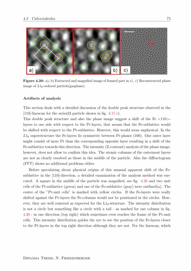
4.3 Cuboctahedra 75
Figure 4.20: a), b) Extracted and magnified image of framed part in c). c) Reconstructed phaseimage of L10-ordered particle(gasphase).
Artifacts of analysis
This section deals with a detailed discussion of the double peak structure observed in the
[110]-linescan for the series23 particle shown in fig. 4.17 c).
This double peak structure and also the phase image suggest a shift of the Fe <110>-
layers to one side with respect to the Pt-layers, that means that the Fe-sublattice would
be shifted with respect to the Pt-sublattice. However, this would seem unphysical. In the
L10 superstructure the Fe-layers lie symmetric between Pt-planes (100). One outer layer
might consist of more Pt than the corresponding opposite layer resulting in a shift of the
Fe-sublattice towards this direction. The intensity (Z-contrast) analysis of the phase image,
however, does not allow to confirm this idea. The atomic columns of the outermost layers
are not as clearly resolved as those in the middle of the particle. Also the diffractogram
(FFT) shows no additional problems either.
Before speculating about physical origins of this unusual apparent shift of the Fe-
sublattice in the [110]-direction, a detailed examination of the analysis method was exe-
cuted. A square in the middle of the particle was magnified, see fig. 4.20 and two unit
cells of the Pt-sublattice (green) and one of the Fe-sublattice (gray) were outlined(a). The
center of the ”Pt-unit cells” is marked with yellow circles. If the Fe-layers were really
shifted against the Pt-layers the Fe-columns would not be positioned in the circles. How-
ever, they are well centered as expected for the L10-structure. The intensity distribution
is not a circle but something like a circle with a tail - as marked for one column in fig.
4.20 - in one direction (top right) which sometimes even reaches the frame of the Pt-unit
cells. This intensity distribution guides the eye to see the position of the Fe-layers closer
to the Pt-layers in the top right direction although they are not. For the linescan, which
Diploma Thesis, N. Friedenberger

76 Results and Discussion
had an integration width of 300 pixels, this could be a problem as well. The software
measures the intensity distribution and weights it over the width of the linescan resulting
in a shifted peak for irregular distributions in the intensity linescans, as it was observed
for the 110-linescan here. For single layer linescans of only a few pixels integration width,
as done for the colloidal series62 particle, this is no problem for the distance measuring, as
long as the smearing is uniform in one direction. Even if the maxima are weighted to the
wrong positions, the relative distance is not influenced. Thus this possible artifact has to
be considered in case of intensity linescans taken over layers staggered against each other.
The strongly oscillating lattice spacing measured in the [110]-direction is an artifact and
no physical phenomenon.
The origin of the irregular intensity distributions at the atom column position has to be
discussed . This effect is stronger for the Fe- than for the Pt-columns. Four explanations
are likely:
1. The nanoparticle rotated by a few degrees during the focal series acquisition.
2. The astigmatism and coma free corrections with the exit wave reconstruction software
are not optimized at this resolution, or the limit of the reconstruction is already
reached.
3. The atoms are not aligned in their columns.
4. This particle might be twinned.
Checking the first and the last image of the focal series confirms point 1. The fringes
in the upper part of the particle are an additional hint for assumption 1. Normally, if the
particle remains perfectly on zone axis there must not be any fringes left. In conclusiona
tilt around the [100]-axis or a twinning have to be considered. The tilt, however, cannot be
large because of the high quality of the FFT. To investigate point 3 tomography combined
with the acquisition of focal series has to be done. Point2 could not be rechecked at this
time.
Concentration gradient - Pt-enriched surface layers?
In the following section the series23 will be discussed in more detail, in order to see whether
there exists a concentration gradient or not. The inner part of the particle has bulk-like
d111-spacings. For the L10-order (in [100]-direction), the <220>-layers should consist of
alternate pure Fe- and pure Pt-layers which is also evident in the phase image (fig. 4.16a).
Layer resolved Lattice Relaxation in Magnetic FexPt1−x Nanoparticles
4.3 Cuboctahedra 77
However, for the bottom part of the particle the order [Dmi03] seems to be worse compared
to the the middle part of the particle. Especially, the last complete surface layer (23 in the
111b-direction) yields a higher Z-contrast (intensity) compared to the inner layers. One
would rather expect a flat envelope of the intensity profile, because the number of Pt- and
Fe-columns in one <111>-layer should be approximately the same and for the edges the
intensity should decrease due to the geometric structure.
This also confirms the model for the Pt-segregation to the surface layers, at least for the
end section of the 111b-linescan. At the beginning the noise in the linescan signal was
relatively high and the intensity signal weak. Presumably the atom columns in that part
of the particle consist mainly of Fe-atoms or of very few atoms.
Also the presence of oxygen as a reason for this relaxation has to be considered [Tro04].
Due to the small Z = 16 of oxygen the phase of the exit wave is hardly visible. XMCD
measurements executed in my group yield a surface oxidation of those particles. Due to
the surface sensitivity of the x-ray magnetic circular dichroism of approximately 3-4 nm
[Ant06a] (in electron yield) it was found, that the particles were oxidized at the surface but
not throughout the whole particle. In conclusion an oxidation of the particles could only
explain larger surface layer spacings but not the observed oscillatory behavior. Within the
framework of my thesis this point could not be investigated further.
Diploma Thesis, N. Friedenberger

78 Results and Discussion
4.3.3 Summary
In this section it was shown that:
1. The averaged lattice parameter of one particle prepared by gasphase condensation
was found to be the same within the errors by three different analysis methods.
2. The averaged lattice constant from several particles <aFFT> = 0.397 ± 0.9% nm is
increased by 4.1% with respect to the FePt bulk value, assuming a fcc lattice.
3. Separation for a and c for one particle shows that a difference as small as 2% in
c(0.383 nm) and a(0.391 nm) of a L10-structure (c/a = 0.98) could be resolved.
4. Surface layer relaxation was only observed for the [111]-direction, the layers in other
directions rather showed an oscillatory behavior as known from bulk surfaces.
5. Too large integration widths over more than one column might lead to artifacts in the
intensity profiles if the reconstruction of the phase image does not yield equally round
intensity distributions. In that case deceptive lattice spacings can be measured.
Layer resolved Lattice Relaxation in Magnetic FexPt1−x Nanoparticles

4.4 Spherical Chemical Disordered FePt Colloids 79
4.4 Spherical Chemical Disordered FePt Colloids
In this section the results of the layer resolved investigations for colloidal FexPt1−x nanopar-
ticles (see section 3.1.2) are presented. According to the ratio of the precursors sample
MO20 should have a 50% Fe and 50% Pt stoichiometries. This value could not be con-
firmed by EDX analysis due to charging effects. The large contamination and the charging
indicate a presence of organic material (surfactants) although the TEM grids for both
samples were washed in acetone to remove dispensable ligands before. The second sample
MO10 yielded no homogenous distribution in size and chemical composition. Charging
again influenced the EDX measurements. An exemplary ratio of 36% ± 5at. %Fe and 64%
± 5at. %Pt was measured, i.e. the nanoparticles have a composition similar to FePt3.
TEM images of both samples are given in fig. 3.2 in the experimental techniques chapter.
Sample MO10 was not homogenous in shape and size, the nanoparticles in sample MO20
had a diameter of 2 - 3 nm.
4.4.1 Lattice Structure
This section first deals with the determination of the mean lattice parameter from the FFT
for both samples and the layer resolved analysis for the series62 particle. From the FFT
measurements the fcc structure was clearly identified. One example for a nice FFT is given
in fig. 4.21 for the series62 particle. The angles between the reflection spots are in very
good correspondence to the literature values for the [011]-direction and deviate by 1.6 %
maximal.
Our experiments in Berkeley exhibited a rate of yield for well- reconstructed particles
of 10% − 20% with respect to the total number of acquired focal series. For the MO20
sample the analysis by exit wave reconstruction did not provide improved results with
respect to the Scherzer images (section 4.4.1). The Scherzer images of the MO10 sample
(fig. 4.22) were analyzed by FFT in addition to the focal series reconstruction to obtain
better statistic information.
Diploma Thesis, N. Friedenberger

80 Results and Discussion
Figure 4.21: : fcc phase identification by FFT analysis. FFT image of the series62 particle. Theyellow angular values are taken from [Wil96], the green are the measured ones. The reflectionsare indicated red.
Layer resolved Lattice Relaxation in Magnetic FexPt1−x Nanoparticles

4.4 Spherical Chemical Disordered FePt Colloids 81
Figure 4.22: Overview of the Scherzer images of sample MO10. The yellow circled particleswere FFT analyzed, see fig. 4.23.
Diploma Thesis, N. Friedenberger

82 Results and Discussion
Figure 4.23: . Lattice parameter a of colloidal particles (fig. 4.22) as resolved from FFTanalysis of the Scherzer images.
Determination of the mean lattice constant
Figure 4.23 displays the results for the FFT analysis of the Scherzer images yielding a mean
value of 0.3945 nm ± 1.1 % for the lattice parameter a. With respect to the bulk values
for FePt and FePt3 this is an enlargement of 3.5% and 1.9%. The FFT analysis of the exit
wave reconstructed images leads to a slightly changed result. Compared to the Scherzer
value the lattice constant a = 0.4001 nm± 0.7 % is enlarged by 1.4 % (fig.4.24). For both
cases the mean value of all series was created by averaging all single series mean values
and the standard deviation concerning the mean value represents the error bar. The FFT
analysis of both the Scherzer images and of the reconstructed images yield an enlargement
of the lattice constant with respect to the bulk. The measured lattice constant is even
enlarged up to 2.1% with respect to the bulk value for Pt a = 0.392 nm [Kit02] (table 4.8).
The two figures 4.22 and 4.24 also display that the values of the lattice constant a for
the different directions are not distributed uniformly around the mean value. Therefore the
enlargement of the lattice constant is determined to be direction independent. From the
FFT analysis of the series62particle a mean lattice constant <aFFT> = 0.4019 nm ± 0.9%
Layer resolved Lattice Relaxation in Magnetic FexPt1−x Nanoparticles

4.4 Spherical Chemical Disordered FePt Colloids 83
Figure 4.24: Lattice constant of colloidal particles averaged over all measured directions in thethe FFT of the exit wave reconstructed phase images.
was obtained. Therefore the mean lattice constant is enhanced by 5.5% with respect to
the FePt-bulk value and by 3.9% with respect to the FePt3-bulk value. It is also enlarged
by 2.5% compared to the lattice parameter for Pt.
Linescan analysis for the series62 particle
According to the good orientation and quality of the reconstructed phase image of the
series62 particle it was further analyzed by linescans. As discussed in section 4.3.2 a large
integration width might lead to artifacts, i.e. an averaging of smaller linescans of smaller
integration width is preferable. For this particle both methods (large integration width
and averaging of smaller integration widths) were performed and compared (table 4.9).
Diploma Thesis, N. Friedenberger

84 Results and Discussion
Figure 4.25: Averaged lattice constant a of series62 particle as resolved from linescans taken inthe four directions indicated in fig. 4.29.
Scherzer EWR series62
average 0.3945nm± 1.1% 0.4001nm± 0.7% 0.3999nm± 0.9%
Fe 0.286 nm 38% 39.9% 39.8%
FePt 0.381 nm 3.5% 5.0% 5.0%
FePt3 0.387 nm 1.9% 3.4% 3.3%
Pt 0.392 nm 0.6% 2.1% 2.0%
Table 4.8: Percentage value of the lattice parameter as resolved from the FFT analysisof the Scherzer and exit wave reconstructed images and from linescan analysis of theseries62 particle compared to different FexPt1−x-bulk values [Lan92, Kit02].
The mean value from the linescans with the large integration width (method one) was
resolved by dividing the distance between the outermost columns by the number of columns
minus one. For the second method (described in more detail in section 4.4.2) all single
d-spacings measured for one direction were averaged. That means the standard deviation
Layer resolved Lattice Relaxation in Magnetic FexPt1−x Nanoparticles

4.4 Spherical Chemical Disordered FePt Colloids 85
with respect to the mean value represents the error bar. In case of a reconstruction with
uniform intensity distributions at the positions of atomic columns equal results are expected
(see section 4.3.2).
Fig. 4.25 shows the mean values of the lattice constant as obtained from the 4 linescan
directions (marked in fig. 4.29) with the larger integration widths (method one). In this
case the mean values for each direction vary by 1% maximum. For the other method
the largest difference is 3.4%. Apart from the [100]-direction the mean lattice constants
determined by the two methods are identical (deviation < 0.4%). This enlargement is
due to different numbers of layers covered by the linescans. For the second method an
additional ”surface layer”, which was not detectable in the ”method one linescan” was
included in the [100]-direction. Neglecting this layer yields a mean lattice parameter of
<als> = 0.4084nm ± 5.5%, i.e. the deviation to method one becomes smaller than 0.9%
for this direction.
The newly calculated mean value for method two <als> = 0.4041 nm ± 0.8% varies by
less than 0.2% from the mean value of method one.
direction a (nm) i. w. (pixels) a* (nm)
100 0.4048 400 0.4146 ± 8.4%
110 0.4014 250 0.4009 ± 2.7%
111a 0.4015 200 0.4029 ± 2.8%
111b 0.4054 300 0.4041 ± 2.0%
all directions 0.4033 ± 0.5% - 0.4056 ± 1.5%
Table 4.9: Averaged line scan analysis of the series62 particle for fourdirections (i.w. = integration width). ”a*”: Mean lattice parameter afrom averaging over several linescans of with a l0pixel integration widtheach.
In conclusion both methods yielded identical mean lattice constants. Furthermore no
artifacts in the reconstructed phase image as found in section 4.3.2 have to be considered
for the further relaxation investigations of surface layer relaxation (compare also fig. 4.33
e)).
Diploma Thesis, N. Friedenberger
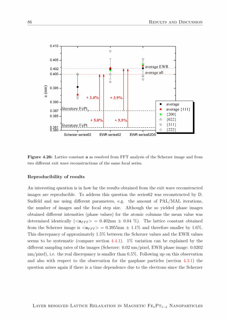
86 Results and Discussion
Figure 4.26: Lattice constant a as resolved from FFT analysis of the Scherzer image and fromtwo different exit wave reconstructions of the same focal series.
Reproducibility of results
An interesting question is in how far the results obtained from the exit wave reconstructed
images are reproducible. To address this question the series62 was reconstructed by D.
Sudfeld and me using different parameters, e.g. the amount of PAL/MAL iterations,
the number of images and the focal step size. Although the so yielded phase images
obtained different intensities (phase values) for the atomic columns the mean value was
determined identically (<aFFT> = 0.402nm ± 0.04 %). The lattice constant obtained
from the Scherzer image is <aFFT> = 0.3955nm ± 1.1% and therefore smaller by 1.6%.
This discrepancy of approximately 1.5% between the Scherzer values and the EWR values
seems to be systematic (compare section 4.4.1). 1% variation can be explained by the
different sampling rates of the images (Scherzer: 0.02 nm/pixel, EWR phase image: 0.0202
nm/pixel), i.e. the real discrepancy is smaller than 0.5%. Following up on this observation
and also with respect to the observation for the gasphase particles (section 4.3.1) the
question arises again if there is a time dependence due to the electrons since the Scherzer
Layer resolved Lattice Relaxation in Magnetic FexPt1−x Nanoparticles

4.4 Spherical Chemical Disordered FePt Colloids 87
images were usually acquired before the focal series. This difference, however, is smaller
than any error bar and not discussed. As already mentioned before this phenomenon has to
be investigated in greater detail, e.g. by successive acquisitions of focal series of the particle.
The obtained reconstructed images have to be tested accurately concerning changes in the
shape of the particles. Those have to be taken into account when speculating about the
reasons for changes in the lattice constant.
SampleMO20
As mentioned above the exit wave reconstruction yielded no improvement in the images
for the MO20 sample. Either the program (TrueImage) had problems with those tiny par-
ticles of 2-3 nm diameter or more probably, the particles were not stable enough under the
electron beam. Only the analysis of three particles in series27 and not of four as indicated
(fig. 4.27) was possible. The particle c in this series shows two directions but could not be
indexed in the FFT. The same problem occured in the series32 and series33 analysis. The
fringes were too weak to identify them in the FFT image. Therefore another check in the
Scherzer images was performed for series32 (indicated as series32S in fig. 4.28).
A FFT analysis of the particles (a, b, d in fig. 4.27) and of the Scherzer image of series32
leads to <aFFT> = 0.3987nm ± 1.6% (1.6% = standard deviation). The error bars in this
analysis are around 4.5% for the single directions, i.e. no accurate determination of the
mean lattice parameter was possible. The obtained values, however, hint at an enlargement
of the lattice parameter again. The mean value is enlarged by 1.7% even with respect to
the Pt-bulk value.
Figure 4.27: Overview of the EWR phase images of sample A1. The (yellow) circles in series27indicate the FFT analyzed particles of this series.
Diploma Thesis, N. Friedenberger
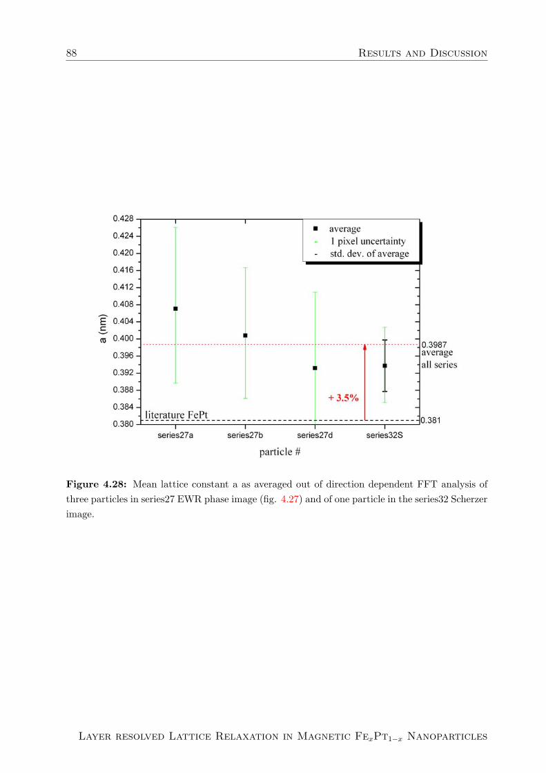
88 Results and Discussion
Figure 4.28: Mean lattice constant a as averaged out of direction dependent FFT analysis ofthree particles in series27 EWR phase image (fig. 4.27) and of one particle in the series32 Scherzerimage.
Layer resolved Lattice Relaxation in Magnetic FexPt1−x Nanoparticles

4.4 Spherical Chemical Disordered FePt Colloids 89
Figure 4.29: Indication of the facets of the (colloidal) series62 particle and of the linescandirections for the relaxation analysis.
4.4.2 Surface Layer Relaxation
Intensity linescans of an integration width of only ten pixels were taken along all four
directions of the series62 particle (fig. 4.29). Due to the the perpendicular directions [110]
and [100] the linescans along the [110]-direction are taken along a <200>-layer and those
along the [100]-direction along a <220>-layer (fig. 4.30). Every single linescan is marked
and numbered in this figure. The d111-layers are numbered as well as shown in the two
bottom images (111a and 111b d-spacing in fig. 4.30). This numeration of the 111-layers
is in accordance to the layer intervals for the relaxation analysis (fig. 4.32 and fig. 4.31).
Along the two other directions, [110] and [100] , the layer numbers in one direction are
chosen identical to the linescan numbers of the perpendicular direction. (The layer numbers
are also marked in 4.32).
The linescans along the 111 directions give the d111-spacing multiplied by a factor three,
because only every third layer (column) is measured. To directly get the d111-spacings from
Diploma Thesis, N. Friedenberger

90 Results and Discussion
the linescans either the integration width has to be increased or three or more successive
linescans have to be averaged. As discussed in section 4.3.2 a large integration width
might lead to artifacts in the determination of the dhkl-layer spacing. Therefore a number
of adjacent 10pixel width linescans of the same length and all covering the same number of
layers was averaged (fig. 4.31) and further investigated. The resulting dhkl-layer spacings
are shown in fig. 4.32.
The error bars for the single d-layer spacings are due to the 1-pixel uncertainty. For the
mean values of the d-layer spacings and the lattice parameter, respectively, the standard
deviation represents the error bar. For the [100]-direction the linescans 8-18 were averaged
and the layer to layer distances determined. The results for this and the two [111]-directions
are shown in table 4.10. The numbers of the layers are not in conformity with those marked
in fig. 4.30. Layer number 1, in [100]-direction, in this sketch is identical to layer number
2 for the relaxation investigations. In conclusion layer number 20 in the investigation is
identical to layer number 19 in the sketch. In fig. 4.31 c) this is indicated. The red numbers
(1-19) show the numeration in the sketch and the black ones (1-20) show the numeration
used for the relaxation analysis.
The additional ”layer” was discovered in the averaged [200]-linescan and was not recognized
by eye in the phase image, i.e. the intensity (phase signal) is weak. DERIP did not detect
this ”layer” as shown in fig. 4.33 f) either. Varying the contrast, shown in the same figure
a)-c), yields at least two additional outermost atom columns (new ”layer” one - best visible
in c)), i.e. this layer is not complete, several atom columns are missing.
It is not clear if it has ever been complete. The atom columns could have also been
moved from other positions of the particle, e.g. from the edges of two surface layers. The
significant missing of edge atomic columns is reported in literature, e.g. [Wan06] and was
also observed for this particle.
According to the phase signal (intensity) the additional ”layer” either contains only a few
atoms or the layer consists mainly of Fe, due to the smaller Z-contrast. Again, the presence
of oxygen has to be considered, too.
Taking the additional layer into account a mean value of <als> = 0.207 nm ± 8.3% is
resolved. With respect to this mean value layer interval 1-2 is increased by 26.7%. The
other outermost layer interval 19-20 is enlarged by 14.5% but in this case, apart from the
edge columns, layer 20 is complete. Neglecting the outermost layer intervals on both sides
of the particle the mean value can be calculated to 0.2023 nm ± 4% which is equal to a
lattice parameter of 0.404 nm ± 4%. The layer intervals between layer 3 and 17 vary around
0.202 nm ± 2.4%. With respect to this value layer interval 17-18 is compressed by 10%.
This interval, however is the only one with d200-layer spacing of 0.1818 nm. Compared to
Layer resolved Lattice Relaxation in Magnetic FexPt1−x Nanoparticles
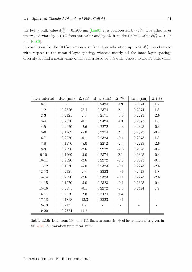
4.4 Spherical Chemical Disordered FePt Colloids 91
the FePt3 bulk value dfcc200 = 0.1935 nm [Lan92] it is compressed by -6%. The other layer
intervals deviate by +4.4% from this value and by 3% from the Pt bulk value dfcc200 = 0.196
nm [Kit02].
In conclusion for the [100]-direction a surface layer relaxation up to 26.4% was observed
with respect to the mean d-layer spacing, whereas mostly all the inner layer spacings
diversify around a mean value which is increased by 3% with respect to the Pt bulk value.
layer interval d200 (nm) ∆ (%) d111a (nm) ∆ (%) d111b (nm) ∆ (%)
0-1 - - 0.2424 4.3 0.2374 1.8
1-2 0.2626 26.7 0.2374 2.1 0.2374 1.8
2-3 0.2121 2.3 0.2171 -6.6 0.2273 -2.6
3-4 0.2070 -0.1 0.2424 4.3 0.2373 1.8
4-5 0.2020 -2.6 0.2272 -2.3 0.2323 -0.4
5-6 0.1969 -5.0 0.2374 2.1 0.2323 -0.4
6-7 0.2070 -0.1 0.2323 -0.1 0.2373 1.8
7-8 0.1970 -5.0 0.2272 -2.3 0.2273 -2.6
8-9 0.2020 -2.6 0.2272 -2.3 0.2323 -0.4
9-10 0.1969 -5.0 0.2374 2.1 0.2323 -0.4
10-11 0.2020 -2.6 0.2272 -2.3 0.2323 -0.4
11-12 0.1970 -5.0 0.2323 -0.1 0.2273 -2.6
12-13 0.2121 2.3 0.2323 -0.1 0.2373 1.8
13-14 0.2020 -2.6 0.2323 -0.1 0.2273 -2.6
14-15 0.1970 -5.0 0.2323 -0.1 0.2323 -0.4
15-16 0.2071 -0.1 0.2272 -2.3 0.2424 3.9
16-17 0.2020 -2.6 0.2424 4.3 - -
17-18 0.1818 -12.3 0.2323 -0.1 - -
18-19 0.2171 4.7 - - - -
19-20 0.2374 14.5 - - - -
Table 4.10: Data from 100- and 111-linescan analysis. # of layer interval as given infig. 4.32. ∆ : variation from mean value.
Diploma Thesis, N. Friedenberger

92 Results and Discussion
layer interval layer interval* dhkl (nm) ∆ (%)
0.5-1.5 1-3 0.2828 -0.3
1-2 2-4 0.2677 -5.6
1.5-2.5 3-5 0.2979 5.1
2-3 4-6 0.2828 -0.3
2.5-3.5 5-7 0.2778 -2.0
3-4 6-8 0.2879 1.5
3.5-4.5 7-9 0.2828 -0.3
4-5 8-10 0.2828 -0.3
4.5-5.5 9-11 0.2828 -0.3
5-6 10-12 0.2778 -2.0
5.5-6.5 11-13 0.2828 -0.3
6-7 12-14 0.2878 1.5
6.5-7.5 13-15 0.2878 1.5
7-8 14-16 0.2828 -0.3
7.5-8.5 15-17 0.2778 -2.0
8-9 16-18 0.2777 -2.0
8.5-9.5 17-19 0.2879 1.5
9-10 18-20 0.2879 1.5
9.5-10.5 19-21 0.2777 -2.0
10-11 20-22 0.2878 1.5
10.5-11.5 21-23 0.2929 3.3
11-12 22-24 0.2727 -3.8
11.5-12.5 23-25 0.2778 -2.0
12-13 24-26 0.2979 5.1
12.5-13.5 25-27 0.2980 5.1
13-14 26-28 0.2879 1.5
13.5-14.5 27-29 0.2727 -3.8
14-15 28-30 0.2778 -2.0
Table 4.11: Data from the 110-linescan analysis. Layerinterval: layer interval with respect to fig. 4.32. Layerinterval*: layer interval with respect to the layer numbersmarked in fig. 4.30. ∆: variation from mean value.
Layer resolved Lattice Relaxation in Magnetic FexPt1−x Nanoparticles

4.4 Spherical Chemical Disordered FePt Colloids 93
For the [111]-directions a significant surface layer relaxation was not observed (fig. 4.31
and table 4.10). The lattice layer spacings randomly spread around the mean value. The
maximum variations from the mean value are +4% for the 111b-direction and -6.6% for
the 111a-direction. In case of the 111b-directions apart from the d-layer spacing of interval
15-16, the value of the other surface layer spacing can be also found in the core of the parti-
cle. In this direction for both surface layers the next layer spacing is increased with respect
to the mean value. Remarkable is the lattice spacing decrease from layer 15-16 down to
layer interval 13-14 by -6.6% over this distance. A similar trend can be found for the layer
intervals 19-20 down to 17-18 in the 100-direction and for the layer intervals 0-1 up to 2-3
for the 111a-direction, respectively. For the second direction the decrease is -11.6%. These
outermost layer spacings can be also found in the middle part of the particle. The mean
curve of all given linescans in the [110]-direction has a profile which is not interpretable
because the local peak shape of the maxima is not unique. Caused by this, the arithmetic
mean value could not be determined (see average curve in fig. 4.31d)). It is easy to find
that all intensity peaks are shifted randomly against each other. A separate averaging of
the even numbered and of the odd numbered linescans was done. Those averaged lines-
cans yielded the d110-layer spacing because only the next but one layers were measured.
In fig. 4.32d) both obtained results were plotted. This leads to a strange numbering of
the layer intervals. It is corrected in table 4.11 with respect to the linescan numbers in
[100]-direction extended by two additional layers non-marked in the image.
The results for the [110] direction differ from those of the other three directions since the
outermost layer intervals have approximately the values of the mean layer spacing (d110 =
0.2835 nm).
The largest d110-layer spacings (d110 = 0.298 nm) are found for the non surface layer in-
tervals 3-5, 24-26 and 25-27. These values are enlarged by 5.1% with respect to the mean
value. Besides, the outer layer intervals are compressed, e.g. 2-4 by -5.6%. A similar be-
havior can be found for the layer intervals 27-29 and 22-24 which are compressed by -8.9%
with respect to the adjacent intervals 25-27 and 24-26, respectively. These correlations hint
at a movement of atom columns in the common layers 27 and 24 towards one preferential
side each. Indeed larger spacings (dark areas) can be seen in fig. 4.29 regarding the area
below the ”111b-arrow”. Due to the mean - along several atom columns - lattice spacings
yielded from the averaged linescans a direct transfer of the obtained spacing information
to the phase image is not possible.
Therefore every linescan has to be analyzed separately to determine the d-layer spacing
which could not be performed in this thesis.
The different spacings can be attributed to the different stoichiometry of Fe and Pt atoms
Diploma Thesis, N. Friedenberger

94 Results and Discussion
in the columns. Figure 4.33 a)-d) shows the identical phase image with different con-
trasts. Image a) displays the different chemical compositions of the atomic columns. Pt
rich columns can be identified by a brighter phase signal. It becomes obvious that the
brightest columns are distributed randomly within the particle, whereas the surface layers
preferably include columns of weaker intensity. This effect is also induced by the almost
perfect truncated octahedron-like structure of the particle. Due to this structure for a
particle of uniform chemical distribution the phase signal is equal for the center columns
and declines approaching the facets of the particle. An example of such an intensity profile
was found in fig. 4.31 b). The small variations are due to the non uniform stoichiometry
and the number of atoms in one column.
direction 100 110 111a 111b
average 0.4146 nm ± 8.3% 0.4009 nm± 2.7% 0.4029 nm±2.8% 0.4041 nm ± 2.0%
Fe100 +45% +40.2% +40.9% +41.3%
Fe50Pt50 +8.8% +5.2% +5.7% +6.1%
Fe25Pt75 +7.7% +3.6% +4.1% +4.4%
Pt100 +5.8% +2.3% +2.8% +3.2%
Table 4.12: Percentage value of the lattice parameter as resolved from the linescan analysis of theseries62 particle compared to different FexPt1−x-bulk values [Lan92, Kit02].
4.4.3 Summary
For the spherical colloidal particles in this section the following can be concluded:
1. A detailed FFT analysis of the reconstructed phase images revealed a mean lattice
constant of 0.400 nm which is enlarged by 3.4% with respect to the FePt3 bulk value.
2. Not conform to the expectation that nanoparticles consist of Pt-enriched surfaces, a
lattice relaxation was only observed for the 100-direction, the layers in other direc-
tions rather showed random distributions.
3. Pt-segregation to the surface layers could not be confirmed by the experimental data.
Layer resolved Lattice Relaxation in Magnetic FexPt1−x Nanoparticles

4.4 Spherical Chemical Disordered FePt Colloids 95
Figure 4.30: Indication of the facets of the series62-particle and of the linescan directions forthe relaxation analysis.
Diploma Thesis, N. Friedenberger

96 Results and Discussion
Figure 4.31: Viewgraph of the linescans taken in the four directions as indicated in fig. 4.30.
Layer resolved Lattice Relaxation in Magnetic FexPt1−x Nanoparticles

4.4 Spherical Chemical Disordered FePt Colloids 97
Figure 4.32: Layer resolved analysis of the four linescans as indicated in fig. 4.30. Here a)shows d200 spacing, b) d111a spacing, c) d111b spacing and d) d110 spacing.
Diploma Thesis, N. Friedenberger
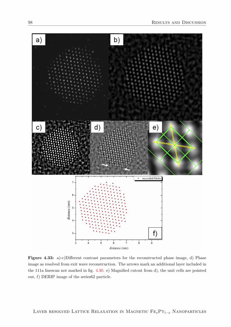
98 Results and Discussion
Figure 4.33: a)-c)Different contrast parameters for the reconstructed phase image, d) Phaseimage as resolved from exit wave reconstruction. The arrows mark an additional layer included inthe 111a linescan not marked in fig. 4.30. e) Magnified cutout from d), the unit cells are pointedout, f) DERIP image of the series62 particle.
Layer resolved Lattice Relaxation in Magnetic FexPt1−x Nanoparticles

4.5 Simply Twinned Particles 99
4.5 Simply Twinned Particles
It is very well known for gasphase particles that they have a tendency to be simply or
multiply twinned for specific conditions (see fig. 6.1)[Dmi03]. Atomistic simulations sug-
gest that multiply twinned structures are energetically favored for small metallic clusters
[Mue05]. Experiments [Sta03c] on gasphase condensated FePt nanoparticles showed mul-
tiply twinned structures up to 5.9 nm diameter while larger particles of 7.6 nm prepared at
higher gas pressures are single crystalline. For wet chemical synthesized FePt nanoparticles
with surfaces modified by organic ligands the single crystallinity down to sizes smaller than
3 nm in diameter has been reported [Sta03a].
During my investigations I found colloidal as well as gasphase-prepared simply twinned
particles. An example is shown in fig. 4.35. a) and b) show the colloidal particle and the
corresponding FFT, c) and d) the gasphase condensated particle and the corresponding
FFT.
Both particles were orientated in the [011]-direction and are twinned along a <111>-plane.
This plane is marked by a (green) box, this box also marks the common [111]-direction.
The arrows show the common <111>-layers (yellow) and the deviating [111]-directions
(red).
Unfortunately the Exit Wave reconstruction was not possible for the colloidal particle and
only two Scherzer images (particle 60*a and 61a) could be recorded (fig. 4.35 a)).
Fig. 4.34 shows the results. A tilt of that particle was observed under the electron beam:
In a different Scherzer image of focal series60 , acquired approximately two minutes be-
fore the Scherzer image series*60, only the upper part of the particle shows lattice fringes,
whereas the analyzed particle of series60*a shows 111-fringes all over the particle. The
twin boundary was observed for the first time in the series61 Scherzer image (fig. 4.22,
particle 61a). The diameter of this particle is approximately 2.5 nm, which is well below
the ”single crystal” limit reported in [Mue05]. As shown in fig. 4.34 the mean value for
the lattice parameter for both Scherzer images is 0.3961nm ± 1%. The lattice parameter
of series61 is increased by 1.4% with respect to the one of series60*. Both values however
are within the error bars. Nevertheless this increase for successive focal series should be
regarded more closely, since a time dependent structural relaxation under the e-beam may
be at its origin.
The FFT analysis was also performed separately for the top and the bottom part of
the particle. Both lattice parameters deviate only by 0.5%.
The mean value of the lattice parameters resolved of other particles in the MO10 sample
are within 0.4% identical to the mean value determined here.
Diploma Thesis, N. Friedenberger

100 Results and Discussion
Figure 4.34: . Lattice parameter for a simply twinned colloidal particle (series61) resolved fromdirectional FFT analysis. The error bar represents the standard deviation.
In fig. 4.14 the mean lattice parameter of the twinned particle prepared by gasphase
synthesis is shown (series16). The diameter of this particle is approximately 7 nm and the
simply twinned structure it is in good accordance to the experimental results mentioned
in [Mue05]. Fig. 4.36 shows that the particle facets are not very well defined. No surface
layer is complete, single atom columns are distributed at the surface facets. It seems that
the bottom <111>-layer interval has a larger d111-layer spacing than the <111>-layers
inside the particle. Due to the small phase signal of this surface layer, its relaxation could
be rather attributed to the presence of oxygen than to a Pt-segregation.
One also notices that the atom columns are not perfectly aligned. This misalignment at
the ends of the layers is also observed for the top <111>-layers.
The displacement of the atom columns is most likely connected to sintering processes (see
fig.6.7). In this figure three successive EWR phase images are presented. Unfortunately,
the orientation of the particles was not stable during the acquisition of three focal series.
The comparison of series16 and series17, however, reveals a changed boundary structure.
Even the bending of layers can be observed.
Layer resolved Lattice Relaxation in Magnetic FexPt1−x Nanoparticles

4.5 Simply Twinned Particles 101
Figure 4.35: Two twinned particles in [011]-zone axis. a) colloidal particle (series61) b) FFTof series61 particle c) gasphase particle (series16) d) FFT of series16 particle
Diploma Thesis, N. Friedenberger
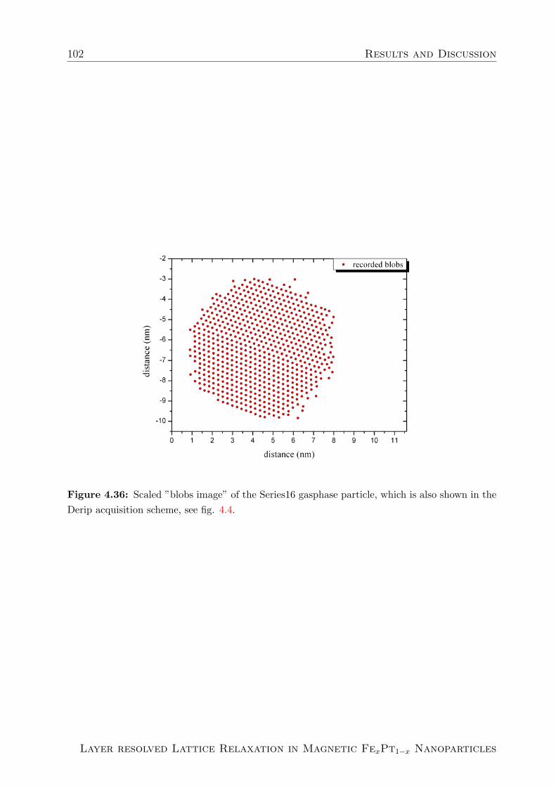
102 Results and Discussion
Figure 4.36: Scaled ”blobs image” of the Series16 gasphase particle, which is also shown in theDerip acquisition scheme, see fig. 4.4.
Layer resolved Lattice Relaxation in Magnetic FexPt1−x Nanoparticles

Chapter 5
Conclusion
The aim of this thesis was to analyze gasphase and wet chemical prepared FexPt1−x
nanoparticles (NPs) with respect to the influence of composition gradients and shell-
wise layered structures on the lattice parameter. High Resolution Transmission Electron
Microscopy (HR-TEM) was used for the analysis. Traditional HR-TEM images (lattice
images) were interpreted by visual inspections. Further improvements included the de-
velopment of indirect methods and a quantitative comparison of simulated images with
experiments. Recently it became possible to recover the full phase and amplitude in-
formation of the electron wave exiting the sample (Exit Wave Reconstruction (EWR))
by recording a focal series of HR-TEM images. With this technique the shape and the
separation of lattice planes could investigated with sub-Angstrom resolution and without
disturbing delocalization effects. To determine the mean lattice parameter of the NPs three
different analysis methods were used and compared to each other. Within the error bars
every method revealed the same result. As a result of this detailed analysis the lattice
structure in different crystallographic directions is presented for one gasphase (fig. 4.18)
and one colloidal (fig. 4.32) NP. It is demonstrated that apparently unphysical results can
be removed by an even more refined analysis and that in focal series tilts or movements of
the particle which are not visible in the FFT may produce such artifacts.
From my analysis no evidence for a surface layer relaxation in general was found. The
layer spacing rather shows small oscillations within the error bar around the mean lattice
parameter of the core. In future investigations more detailed statistic analysis of the sur-
face relaxation may have to be done, to clarify the existence of a surface relaxation in FePt
nanoparticles. One should note, however, that my detailed investigations revealed that no
particle is like the other.
A general lattice expansion of up to 4% compared to the bulk was determined. The origin
Diploma Thesis, N. Friedenberger

104 Conclusion
of this expansion could not be identified. The presence of oxygen may play a role. On
the other hand the lattice expansion in the NPs may be driven by surface effects. Due
to the limitation of the nanoparticle there might be a ”surface relaxation” as observed in
metallic bulk systems throughout the particle. To investigate this in more detail, the three
dimensional shape and the atomic composition of the NPs must be known. In conclu-
sion the combination of quantitative HR-TEM using the Z-dependence of the phase signal,
EWR and tomography, as discussed in this thesis is a promising method to fully reveal the
structure of NPs.
Layer resolved Lattice Relaxation in Magnetic FexPt1−x Nanoparticles

Chapter 6
Appendix
A-1 Microscope Parameters
Table 6.1: specific microscope parameters
microscope CM300 TecnaiF20 ST
voltage (kV) 300 200
electron wavelength (pm) 1.97 2.51
CS (mm) 0.6 1.2
semiconvergence angle α (mrad) 0.2 0.1
defocus spread (nm) 1.5 10
information limit (nm) 0.08 0.15
sampling rate (A/pixel) 0.202 0.216
A-2 Structural Data for FePt
Calculation of dhkl for fcc and fct structures
fcc:
dhkl =a√
h2 + k2 + l2(6.1)
fct:
1/dhkl =
√h2 + k2
a2+l2
c2(6.2)
Diploma Thesis, N. Friedenberger
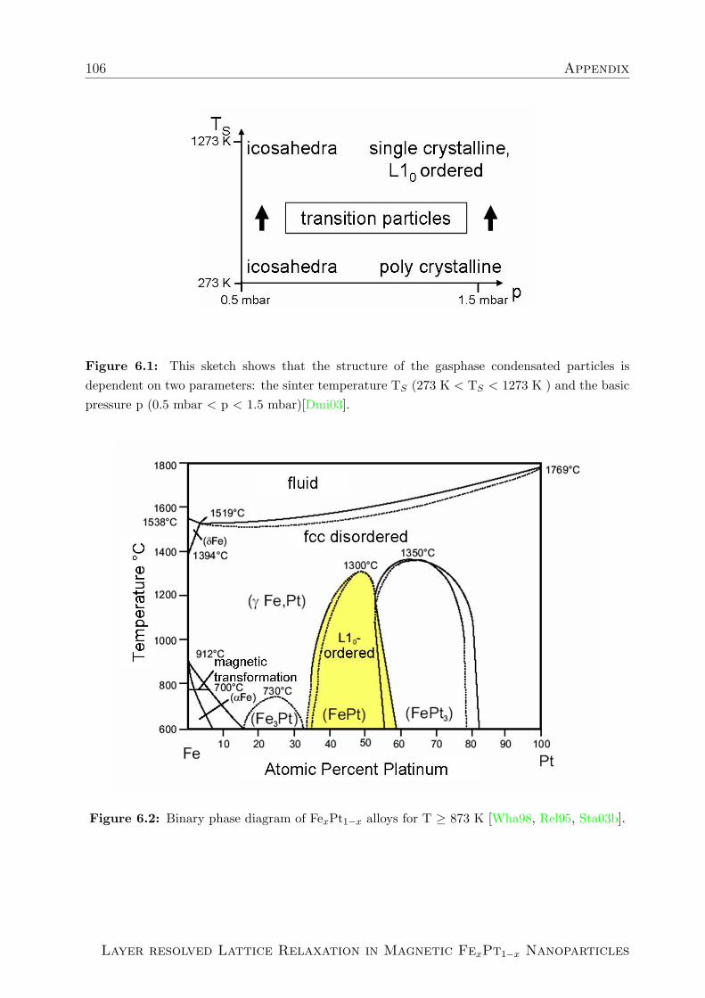
106 Appendix
Figure 6.1: This sketch shows that the structure of the gasphase condensated particles isdependent on two parameters: the sinter temperature TS (273 K < TS < 1273 K ) and the basicpressure p (0.5 mbar < p < 1.5 mbar)[Dmi03].
Figure 6.2: Binary phase diagram of FexPt1−x alloys for T ≥ 873 K [Wha98, Rel95, Sta03b].
Layer resolved Lattice Relaxation in Magnetic FexPt1−x Nanoparticles

A-2 Structural Data for FePt 107
Figure 6.3: Sketch of a truncated octahedron (a) and of a cuboctahedron (b) (adapted from[Sta03b]. In (a) a cut along a <110>-layer is displayed by red lines. NP are often observed tobe orientated along a [110]-zone axis, i.e. [111]-facets and [100]-facets are found at the edges.The NPs also tend to have [110]-facets due to the missing of the edge atom columns between two[111]-facets.
Figure 6.4: Indication of facets for a truncated octahedric particle.
Diploma Thesis, N. Friedenberger

108 Appendix
Figure 6.5: Schematic view of the L10-structure. Fe- and Pt- atom layers alternate along the[001]-direction. The structure is tetragonal distorted (c < a due to the different atom radii of Feand Pt). Adapted from [Sta03b].
Figure 6.6: Diffraction pattern for fcc single crystalline structures along the [100]-zone axis (a)and along the [110]-zone axis (b). The reflections are marked by different colors for differentdirections. The red marked reflections are only visible in the L10-structure and are forbidden forthe disordered fcc structure. Adapted from [Sta03b].
Layer resolved Lattice Relaxation in Magnetic FexPt1−x Nanoparticles

A-2 Structural Data for FePt 109
fcc (a = 0.381 nm) fct (a = 0.385 nm, c = 0.371 nm)
h k l dhkl (nm)
1 0 0 -
0 1 0 -
0 0 1 -
1 1 0 -
1 0 1 -
0 1 1 -
1 1 1 0.2200
2 0 0 0.1905
0 2 0 0.1905
0 0 2 0.1905
2 1 0 -
1 0 2 -
0 1 2 -
2 0 1 -
1 2 0 -
0 2 1 -
2 2 0 0.1347
2 0 2 0.1347
0 2 2 0.1347
h k l dhkl (nm)
1 0 0 0.3850
0 1 0 0.3850
0 0 1 0.3710
1 1 0 0.2722
1 0 1 0.2671
0 1 1 0.2671
1 1 1 0.2195
2 0 0 0.1925
0 2 0 0.1925
0 0 2 0.1855
2 1 0 0.1722
1 0 2 0.1671
0 1 2 0.1671
2 0 1 0.1710
1 2 0 0.1722
0 2 1 0.1710
2 2 0 0.1361
2 0 2 0.1336
0 2 2 0.1336
Table 6.2: Calculated dhkl-layer spacing of the allowed miller indices for stoichiometric FePtbulk (fcc and fct structure) [Lan92].
Diploma Thesis, N. Friedenberger

110 Appendix
A-3 Sintering
Figure 6.7: Three exit wave reconstructed phase images of three successive focal series showingthe same NPs. The time frame for the acquisition of the three series is approximately 8 minutes.In series15 only the right of the two nanoparticles clearly visible in the other two series is shown.Sintering of the nanoparticles can be observed.
Layer resolved Lattice Relaxation in Magnetic FexPt1−x Nanoparticles

A-4 Analysis by FFT of Linescans 111
A-4 Analysis by FFT of Linescans
Figure 6.8: FFT analysis for two different averaged linescans for the identic scandirection.
Diploma Thesis, N. Friedenberger

112 Appendix
A-5 EWR Using TrueImage
The TrueImage software is continously improved. The general information given here is
typical for all software versions. At NCEM I used version 2.4.4. It is always helpful to
have a look in the corresponding manual, too.
A-5.1 Focal-series acquisition at the TEM
Before starting for a focal series acquisition the microscope has to be carefully aligned to
the optimum. That means gun tilt and gun shift routines have to be done, the sample has
to be set to the eucentric height, condenser and objective astigmatism has to be corrected
as well as the 2-fold-astigmatism and coma (if possible). Also the pivot points have to be
checked. Since those procedures are slightly different for each microscope no more detailed
information will be given in this context. There is always some help-menu in the software
of the microscopes where all steps can be looked up. The CM300 microscope at NCEM
also has some special software as an additional script in the DigitalMicrograph programm
for correcting astigmatism and coma more easily.
A-5.2 EWR with TrueImage
In Figure 6.9 the control panel of the the TrueImage version used @NCEM is shown. On
the right side the images will be loaded and shown. On the left side are the parameter
settings, the correction and the output options. They are described in a little more detail
in the according sections.
Renaming the file extension
The first thing to do before enabling the TrueImage options is to change the file extension
to ”.dm2” of the uploaded focal series. Note that the image acquisition computer is a
Macintosh which does not export file extensions. Another reason is, that @ the CM300
microscope not the TrueImage acquisition software is used, but also a script for DigitalMi-
crograph which exports the recorded images as ”.dm2” files. Since TrueImage is a software
working on a ”Windows”-system this annoying step has to be done. The easiest way to do
this is to use the ”DOS-shell”. There it’s possible to change the file extensions of whole
folders. Only a few short instructions are necessary:
1. open ”command prompt”: start → programs → accessories → command prompt
Layer resolved Lattice Relaxation in Magnetic FexPt1−x Nanoparticles

A-5 EWR Using TrueImage 113
Figure 6.9: TrueImage control panel for version 2.4.4 as it is displayed when TrueImage isopened.
Diploma Thesis, N. Friedenberger

114 Appendix
(in the German Windows version: Start → Programme → Zubehor → Eingabeauf-
forderung accordingly)
2. choose the partition of your hard disc where the folders with the focal series images
are stored, typically ”C:” or ”D:” by entering C: (D:), then press ”return”
3. change directory to the folder address: cdt”C: · · ·.foldername” press ”return”
4. now you are in that folder: enter: rename *.*t*.dm2 press return
5. if more folders have to be changed the ↑-button can be used, then former commands
are shown by simply pressing it several times; another possible command is: cdt..
which allows for going to one directory above.
remark:t means blank
Convert data
Important: The files have to be numbered sequently starting with 001.extension. TrueIm-
age needs data in Raw- or in Tietz-Format which means .dat extension of the files. So the
images in dm2-format have to be converted. This can be done with the ”Convert Digital
Micrograph Files”-button which appears when the ”tools”-option is selected as shown in
figure 6.10. As soon as this option is checked another window will open. Here the folder
of the focal series is to be selected first, then the first picture with extension ”...001.dm2”
which will appear in this window has to be marked and then the form ”variable header
.dat” has to be chosen. Once the focal series is converted into the .dat-format it can be
loaded into TrueImage under ”File”. Load the focal series. See Figure 6.11. As before also
the first image of that series has to be selected. Now, the first image of the focal series will
be opened in the Display-area. The up/down-arrows can be clicked to display the next or
previous image of the serious. ”Play Movie” allows continuous displaying.
Setting center of reconstruction area
Having all images of the focal series checked the center of the reconstruction area has
to be defined. This is done by clicking in the center of the image in an older version of
TrueImage, in the version used at Berkeley ”Select Area” had to be used. In this version
the advantage is that you can see this selected area also by changing the image numbers.
So it is possible to make sure that your area of interest stays in the frame. Make sure that
the frame is not set too close to the edge of the image. Due to the point-spread-function
Layer resolved Lattice Relaxation in Magnetic FexPt1−x Nanoparticles

A-5 EWR Using TrueImage 115
Figure 6.10: ”tools”-options in TrueImage: changing of file extensions and converting of DigitalMicrograph (.dm-files) into .dat-files is possible.
Figure 6.11: ”files”-options in TrueImage: Loading of a focal series, opening/saving of projectsand import of wave functions and parameter sets is possible.
Diploma Thesis, N. Friedenberger

116 Appendix
(chapter 2.1.3) the information is not complete in the border area of an image and this
leads to errors in the reconstruction. If the object drift is too strong, so that the structure
moved out of the field of view during the focal series acquisition only a reduced number
of images can be used for the reconstruction, however there have to be at least ten images
for TrueImage to work.
Scaling of the gray levels
Once the series is loaded, check ”Histogram - Full Area”(see fig. 6.12) to get the histogram
of the displayed image. Two red lines indicate the minimum and maximum of the gray
levels used for the display. By click and drag (left mouse button) the display minimum and
maximum can be individually redefined as indicated with the two blue arrows in fig. 6.12.
This redefinition will set all images of the focal series to the same normalized minimum
and maximum.
Microscope Parameters
Press ”Set Microscope Parameters” so that the Microscope Parameter window opens and
edit it for the relevant microscope. In fig. 6.9 this window is opened (left side) with
parameters for the CM300 microscope. The parameters to edit are:
HT: High Tension of the microscope in kV
Cs: Spherical Aberration of the objective lens of the microscope in mm
Focus Spread/Information Limit: Usual edit is the information limit which is deter-
mined by the High Tension and the focus spread of the microscope. The focus spread
value corresponds to one half of the (1/e)-width of a Gaussian distribution of foci
[Kub03].
MTF: Modulation Transfer Function of the CCD, has to be 1 for simulations.
Imaging Parameters
Press ”Set Imaging Parameters” so that the Imaging Parameter window opens. In fig.
6.13 left side this window is shown for the CM300 parameters.
Sampling: pixelsize in nanometers. It has to be rechecked regularly since the camera
magnification has to be very accurate.
Layer resolved Lattice Relaxation in Magnetic FexPt1−x Nanoparticles

A-5 EWR Using TrueImage 117
Figure 6.12: Area of the TrueImage control panel in which the scaling of the gray levels for allimages of a series can be done. ”Play Movie” allows for playing back all images continuously.
Diploma Thesis, N. Friedenberger
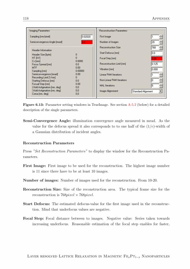
118 Appendix
Figure 6.13: Parameter setting windows in TrueImage. See section A-5.2 (below) for a detaileddescription of the single parameters.
Semi-Convergence Angle: illumination convergence angle measured in mrad. As the
value for the defocus spread it also corresponds to to one half of the (1/e)-width of
a Gaussian distribution of incident angles.
Reconstruction Parameters
Press ”Set Reconstruction Parameters” to display the window for the Reconstruction Pa-
rameters.
First Image: First image to be used for the reconstruction. The highest image number
is 11 since there have to be at least 10 images.
Number of images: Number of images used for the reconstruction. From 10-20.
Reconstruction Size: Size of the reconstruction area. The typical frame size for the
reconstruction is 768pixel × 768pixel.
Start Defocus: The estimated defocus-value for the first image used in the reconstruc-
tion. Mind that underfocus values are negative.
Focal Step: Focal distance between to images. Negative value: Series taken towards
increasing underfocus. Reasonable estimation of the focal step enables for faster,
Layer resolved Lattice Relaxation in Magnetic FexPt1−x Nanoparticles

A-5 EWR Using TrueImage 119
better reconstruction results. See below for how to estimate the defocus values and
the focal step size.
Reconstruction Limit: sets the limit for the reconstruction calculation. Should be equal
to the information limit of the microscope. A slightly larger value is also possible.
Vibration: Vibration amplitude (one half of the (1/e)-width) for mechanical or electrical
vibration in nm. Vibrations are considered to be isotropic but normally the value is
set to zero. (No mechanical vibrations)
Linear PAM Iterations: Maximum number of pure PAM-iterations (see 2.2.2. Usually
it is only used for faster convergence and is set to 2 at most.
Non-Linear PAM Iterations: Number of non-linear PAM-iterations. Usually 0.
MAL Iterations: Number of Mal-iterations also taking non-linear contributions fully into
account. See 2.2.2 for more information on the MAL-method. Typically are 4itera-
tions, but increasing the number up to 10 iterations is mostly more sufficient.
Image Alignment: Usually set to standard alignment for, here a cross-correlation be-
tween the images is initialized to compensate drift. For simulation data ”no image
alignment” has to be selected.
Finding the right defocus values
Finding the defocus values is done with another program: MacTempas which unfortunately
only works on Macs. There exists ”Focus Determination” in the ”Process”-menu in which
can be chosen between the general parameter setting ”Find Focus Search Parameters”
(see fig. 6.14) and ”Find Focus From Image” (see fig. 6.15). So it is reasonable to set
the parameters first. The CM300-parameters are given in tab. 6.1. Also the inner peak
should be excluded for the fitting procedure and maximum use of 3 peaks works well. Mind
that the full defocus range of the series is be taken into account in the interval of smallest
defocus and largest defocus, better determine this interval broad-minded. So for the focal
series taken around CM300’s Lichte-defocus which is approximately −2700A the interval
given in fig. 6.14 is unusable. More specifications can be done in ”Peak Finding Criteria”.
As soon as all parameters have been set and the image whose defocus has to be estimated
is opened, ”Find Focus Search Parameters” has to be selected and a window as shown in
fig. 6.15 appears. The ”Make CTF follow ring markers”-box has to be checked then
the calculated CTF due to the input parameters has to be fitted to the peak. The more
Diploma Thesis, N. Friedenberger

120 Appendix
Figure 6.14: Window for setting the parameters defocus values in MacTempas. Here theparameters for the defocus-fitting can be set, so that they will be transferred to every focus-finding-process.
accordance between the both the more precise is the estimated defocus value. Look for
the minima to optimize accordance. It is important not to weight the first maximum to
strong, better go for the next ones. The calculated CTF (red-colored graph in figure) can
be shifted by clicking and holding one of the numbered red lines that indicate the maxima.
The defocus value is shown in the middle of that window.
Focal-Step-Size Analysis
If the defocus determination is done for every image in a focal series a plot can be made
∆f(image no.). The slope of the linear fit is the focal-step-size. These plots enable also to
see the images whose defocus values differ too far from the fit and might be unusable for
the reconstruction. Depending of the quality of the focal series images a smaller amount
of images leads to a better result concerning the focal-step-size.
Check Input Parameters + Start Reconstruction
There are different checking options as to check the CTF referring to your input parameters.
Therefore ”Show CTF” has to be checked. In this CTF window another option can be
checked: ”FFT” to display a rotationally averaged line profile of the FFT. ”FFT-Peak”
allows for displaying the maximum intensity of the FFT for each radius. But the most
important thing to check is your general parameters. To do this, ”Test Mode” under
”Start Reconstruction” has to be checked and ”Check Parameters” has to be activated.
Layer resolved Lattice Relaxation in Magnetic FexPt1−x Nanoparticles

A-5 EWR Using TrueImage 121
Figure 6.15: Focus Control in MacTempas. Defocus Determination is done as described inA-5.2. The other parameters on the right side are microscope-specific and define the form of theCTF. The defocus value is the unknown parameter in the CTF and is therefore estimated throughthis fitting process. The small square image in the right top corner of the inner box shows theCTF calculated from the image and in the small brighter angular range the CTF based on theinput parameters.
Figure 6.16: Defocus determination for sample.
Diploma Thesis, N. Friedenberger

122 Appendix
Then the programme tests the input parameters. If nothing appears in the window on the
left side, ”Show FSR Warning” in the ”Display Selection” has to be checked before, the
reconstruction can be started. Therefore ”Test Mode” has to be unchecked.
Reconstruction Results
When the reconstruction is finished the results have to be checked carefully before any aber-
ration correction should be done. ”Show FSR Convergence” gives you the mean square
error, it should be lower than 0.01 for an optimal reconstruction, but that is hardly achiev-
able for nanoparticles. Also the ”Focus Step Analysis” should be compared to the input
value. If it differs too strongly, the reconstruction has to be restarted with the corrected
value. Also it is advisable to check the defocus value in the ”Aberration Correction”-section.
Therefor different steps have to be done:
1. choose the ”lens” in the ”Tool Box”, click on the display, repeat till display only
shows the area of interest of the structure. Important: Make sure that ”Phase
of Wave Function” or ”Amplitude of Wave Function” is checked in the ”Display
Selection”.
2. select ”Histogram - Display Area”
3. vary ”Defocus” in the ”Aberration Correction” till the standard deviation in the
histogram is minimal for the ”amplitude”-image or maximal in the ”phase”-image of
the wave function
4. add this defocus-value (mind the algebraic sign) and add it to the start defocus value
in ”Set Reconstruction Parameters”
5. rerun the reconstruction
Now the results have to be checked again. If the mean square error is acceptable, the
step size analysis matches with the input value and the defocus value has not to be corrected
once again, the other aberration corrections can be proceeded.”Aberration Correction” has
to be checked. Here 2-fold astigmatism, coma and 3-fold astigmatism can be corrected.
The procedure is the same as it is in 3.: Maximize standard deviation for phase-image and
minimize for amplitude image. It is recommended to start with the amplitude-image. If
the standard deviation is stable for a huge range, change to the phase-image for further
corrections. Mind that all corrections have to be done in a reasonable array: Of course
it is possible to correct coma with a value of more than 1000 nm, but this would mean
Layer resolved Lattice Relaxation in Magnetic FexPt1−x Nanoparticles

A-5 EWR Using TrueImage 123
Figure 6.17: ”Aberration Correction”in TrueImage: Correcting defocus, 2- and 3-fold astigma-tism and coma is possible. If ”Auto Update” is checked the image currently in the display will beupdated automatically due to every correction step. An automatic estimation and coma is alsopossible.
the microscope was not very well aligned and so the efficiency of the reconstruction is
questionable. There are no fixed values for the maximum correction values, yet experience
has provided the following clues for maximal values:
2-fold astigmatism: 5 nm
3-fold astigmatism: 150 nm
coma: 500-700 nm
Iterative correction of the three values is also strongly recommended. Figure 6.17 shows
the display for the ”Aberration Correction”.
Diploma Thesis, N. Friedenberger

124 Appendix
Figure 6.18: ”Fourier Filter Selection”-window in TrueImage: Choosing of two different or noFourier Filter is possible.
Using Filters
After finishing the correcting procedure the reconstructed image can be ”made perfect”
using a filter, that means to cut off the high- and low-frequencies which could not be
included in the reconstruction anyway. Attend: The lower the number of images used for
the reconstruction the more the low-frequency limit is shifted to higher spatial frequencies.
To use the filters check ”Fourier Filter Selection” and the ”filter-display” opens as shown
in fig. 6.18. Besides ”No Fourier Filter” there are the options: ”Gaussian” and ”Top
Hat” which is usually used. The low- and high-frequency limits can be taken from the
”.mal.log-file” see Saving Files. The high-frequency level is due to the reconstruction
process a little bit larger than gmax, the info limit of the microscope but can be also set to
this value without making the result worse.
Saving Files
In the older version of TrueImage a file name for the reconstruction will be asked before
starting the reconstruction. This was not the case for the version of TrueImage I used
@NCEM: Here the files had to be named afterwards, when saving the whole project or
exporting some different files. Different output files will be generated, unfortunately the
extensions differ between the different versions of TrueImage, the following list explains
Layer resolved Lattice Relaxation in Magnetic FexPt1−x Nanoparticles

A-5 EWR Using TrueImage 125
the extensions of my used TrueImage version (Version 2.4.4 according to header info in
”.mal.log”-file).
.dxy: text file of image alignment and displacement data
.ewf: reconstructed electron wave function (exit wave)
.mal.log: test file with information on dampening fuctions, high- and low-frequency re-
construction limits and with positional alignment tables for each iteration step
.mse: text file with the mean square error of the wave function
.step.log: detailed information on focal step analysis, text file
.ti: Project files, such as files with extension ”.fti” in a former TrueImage version
To save the files check ”File” and then ”Save Project as”. All the files named in the
description are generated. Then it is also possible to save different parameter files, this
option can be found in the” Export”-menu. ”File” also allows for import other projects,
wave functions and parameterfiles as can be seen in fig. 6.11. In ”Output Options”, which
is shown in fig. 6.19, some settings for the output can be made. There is also the possibility
of adding an extra phase-shift. Usually the phase- and amplitude-images are exported in
the .tif-format.
It is also possible to export only the display-area. According to the manual this is
possible with the ”Area Selection”-option. The area defined there should be the area
which is exported. By clicking on the display with the right mouse-button there is also
the possibility of direct .bmp-export of the displayed area. ”Working” in the display can
be done with the tools from the ”Tool Box” which is in analogy to the DigitalMicrograph
tools.
Closing Remark
This short manual for dealing with TrueImage Professional based on my experiences gives
only a few hints for a succesful reconstruction and does not claim to be complete or 100%
perfect. For more detailed information it is strongly recommended to read the relevant
manual for the used version of TrueImage. Especially this version has some features as
”Show Argand Plot” or ”Subtact Vacuum Wave” which were specially programmed for
NCEM and not a part of the normal TrueImage versions. A figure of the TrueImage
control panel (fig. 6.20) with an opened EWR-project is shown to close this chapter.
Diploma Thesis, N. Friedenberger

126 Appendix
Figure 6.19: ”Output Options”in TrueImage.
Layer resolved Lattice Relaxation in Magnetic FexPt1−x Nanoparticles
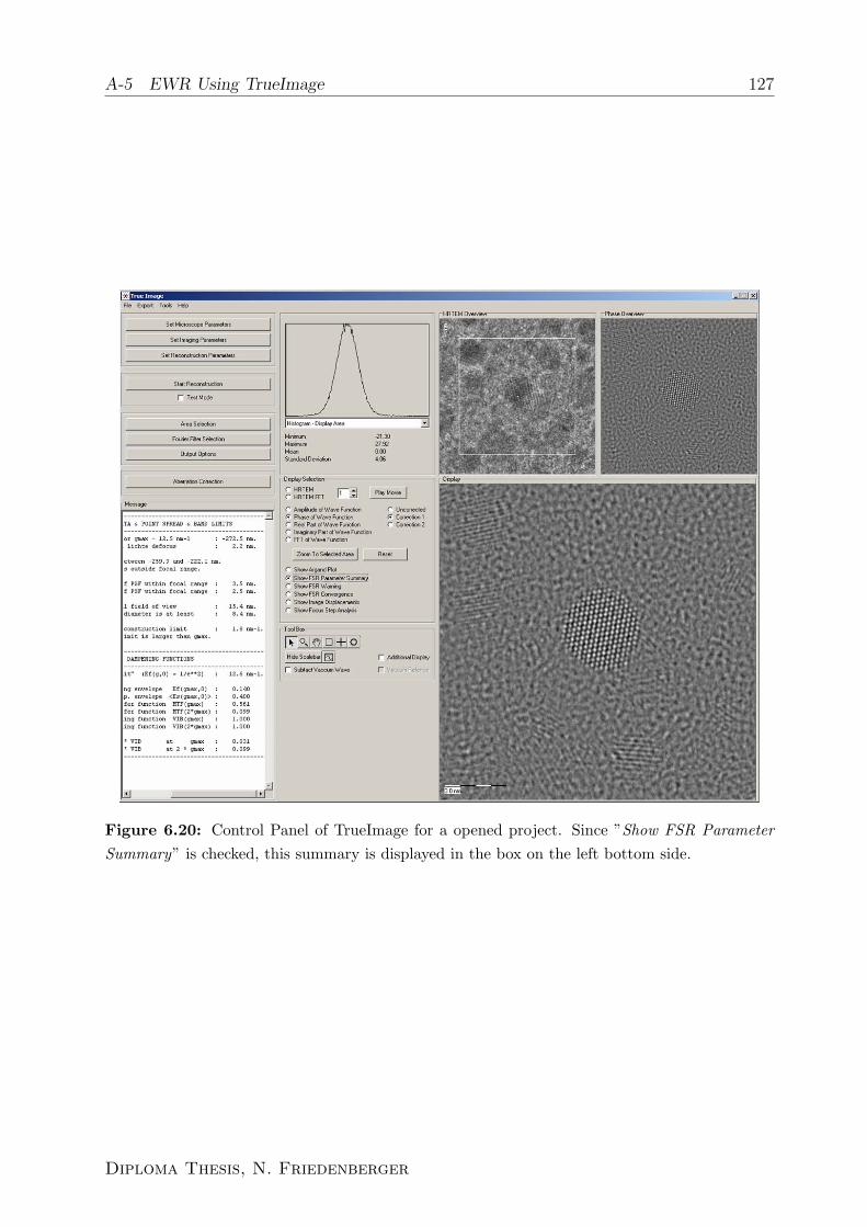
A-5 EWR Using TrueImage 127
Figure 6.20: Control Panel of TrueImage for a opened project. Since ”Show FSR ParameterSummary” is checked, this summary is displayed in the box on the left bottom side.
Diploma Thesis, N. Friedenberger

128 Appendix
Layer resolved Lattice Relaxation in Magnetic FexPt1−x Nanoparticles

Bibliography
[Ace05] M. Acet, C. Mayer, O. Muth, A. Terheiden, and G. Dyker, Formation of extended
ordered monolayers of FePt nanoparticles , Journal of Crystal Growth 285, 365
(2005).
[Ant06a] C. Antoniak, private communication (2006).
[Ant06b] C. Antoniak, J. Lindner, M. Spasova, D. Sudfeld, M. Acet, M. Farle, K. Fauth,
U. Wiedwald, H.-G. Boyen, P. Ziemann, F. Wilhelm, A. Rogalev, and S. Sun,
Enhanced orbital magnetism in Fe50Pt50 nanoparticles , Phys. Rev. Lett. 97,
117201 (2006).
[Bal06] S. Bals, G. V. Tendeloo, and C. Kisielowski, A New Approach for Electron To-
mography: Annular Dark-Field Transmission Electron Microscopy , Adv. Mater.
18, 892 (2006).
[Boo00] C. B. Boothroyd, Quantification of high-resolution electron microscope images
of amorphous carbon, Ultramicroscopy 83, 159 (2000).
[Boo03] C. B. Boothroyd and M. Yeadon, The phonon contribution to high-resolution
electron microscope images , Ultramicroscopy 96, 361 (2003).
[Boo05] C. B. Boothroyd and R. E. Dunin-Borkowski, The contribution of phonon scat-
tering to high-resolution images measured by off-axis electron holography , Ultra-
microscopy 98, 115 (2005).
[Coe96] W. M. J. Coene, A. Thust, M. O. de Beeck, and D. V. Dyck, Maximum-likehood
method for focus-variation image reconstruction in high resolution transmission
electron microscopy , Ultramicroscopy 64, 109 (1996).
[Cow57] J. M. Cowley and A. F. Moodie, The Scattering of Electrons by Atoms and
Crystals. I. A New Theoretical Approach, Acta Cryst. 10, 609 (1957).
Diploma Thesis, N. Friedenberger

130
[Dmi03] O. Dmitrieva, Hochauflosende Elektronenmikroskopie und Kontrastsimulation
zur Strukturaufklarung an gesinterten FePt-Nanopartikeln, Diplomarbeit, Uni-
versitat Duisburg-Essen (2003).
[Dmi06a] O. Dmitrieva, private communication (2006).
[Dmi06b] O. Dmitrieva, M. Acet, J. Kastner, G. Dumpich, C. Antoniak, and M. Farle, J.
Phys. D: Appl. Phys. (2006).
[Dmi06c] O. Dmitrieva, M. Acet, J. Kastner, G. Dumpich, and W. .Wunderlich, J. Nanop.
Res. 1 (2006).
[Dyc96] D. V. Dyck, H. Lichte, and K. van der Mast, Sub-Angstrom structure charac-
terisation: the Brite-Euram route towards one angstrom, Ultramicroscopy 64, 1
(1996).
[ea04] W. et al., J. Appl. Phys. 95 (5) (2004).
[Fc06] FEI-company, FEI Software Overview , (2006).
[Gro99] H. B. Groen, Interface dislocation patterns studied with High Resolution TEM ,
Doktorarbeit, Reichsuniversitat Groningen (1999).
[How63] A. Howie, Proc. R. Soc. A 275, 268 (1963).
[Ish80] K. Ishizuka, Contrast transfer of crystal images in TEM , Ultramicroscopy 5, 55
(1980).
[Jin02] J. R. Jinschek, C. Kisielowski, T. Radetic, U. Dahmen, M. Lentzen, A. Thust,
and K. Urban, Quantitative HRTEM investigation of an obtuse dislocation re-
action in gold with a Cs corrected microscope, in Nanostructured Interfaces.
Symposium (Mater. Res. Soc. Symposium Proceedings Vol.727), pp. 3–8 (2002).
[Kub03] C. Kubel, D. Tang, T. Fliervoet, and A. Thust, TrueImage Professional - Step-
by-Step Guide (Version 1.0.1 Beta) (2003).
[Kila] R. Kilaas, MacTempas User Manual .
[Kilb] R. Kilaas, MacTempasX , http://www.totalresolution.com/ .
[Kir84] E. J. Kirkland, Improved High resolution Image Processing Of Bright Field Elec-
tron Micrographs , Ultramicroscopy 15, 151 (1984).
Layer resolved Lattice Relaxation in Magnetic FexPt1−x Nanoparticles

Bibliography 131
[Kis] C. Kisielowski, E. C. Nelson, C. Song, R. Kilaas, and A. Thust, Aberration
corrected Lattice Imaging with Sub-Angstrom Resolution, Microscopy and Mi-
croanalysis, Supplement 2, 6, 2000, 16 .
[Kis02] C. Kisielowski and J. R. Jinschek, On the feasibility to investigate point defects
by advanced electron microscopy , in 4th Symposium on non-stoichiometrc III-V
compounds, Asilomar, CA (2002).
[Kis06a] C. Kisielowski, Electron Crystallography , pp. 17–29, Springer (2006).
[Kis06b] C. Kisielowski, private communication (2006).
[Kit02] C. Kittel, Einfuhrung in die Festkorperphysik 13. Auflage, Oldenbourg Munchen
(2002).
[Lan92] H. Landolt and R. Bornstein, Landolt-Boernstein New Series IV/5e, Springer
Berlin (1992).
[Lic91] H. Lichte, Optimum focus for taking electron holograms , Ultramicroscopy 38, 13
(1991).
[Mal97] J.-O. Malm and M. O’Keefe, Deceptive ”lattice” spacings in high-resolution mi-
crographs of metal nanoparticles , Ultramicroscopy 68, 13 (1997).
[Mue05] M. Mueller and K. Albe, Lattice Monte Carlo simulations of FePt nanoparti-
cles: Influence of size, composition, and surface segregation on order-disorder
phenomena, Phys. Rev. B 72, 094203 (2005).
[O’K01a] M. A. O’Keefe, Microscopy and Microanalysis 7, 916 (2001).
[O´K01b] M. A. O´Keefe, C. J. D. Hetherigton, Y. C. Wang, E. Nelson, J. H. Turner,
C. Kisielowski, J. O. Malm, R. Mueller, J. Rignalda, M. Pan, and A. Thust,
Sub-Angstrom high-resolution transmission electron microscopy at 300 keV , Ul-
tramicroscopy 89, 215 (2001).
[Rei84] L. Reimer, Transmission Electron Microscopy , Springer Berlin Heidelberg
(1984).
[Rel95] B. Rellinghaus, J. Kastner, T. Schneider, E. F. Wassermann, and P. Mohn,
Thermodynamic analysis of Fe72Pt28 Invar , Phys. Rev. B 51, 2983 (1995).
Diploma Thesis, N. Friedenberger

132
[Rel03] B. Rellinghaus, S. Stappert, M. Acet, and E. F. Wassermann, J. Magn. Magn.
Mater. 266, 142 (2003).
[Sch05] P. Schlossmacher, A. Thesen, and G. Benner, A record-breaking new transmis-
sion electron microscope comes close to achieving the theoretical limit of image
resolution, Carl Zeiss SMT, European Semiconductor 27 (3) (2005).
[Sev03] D. Severin, Diplomarbeit, Universitat Duisburg (2003).
[Sid] M. V. Sidorov, ctfExplorer , http://clik.to/ctfexplorer .
[SM04] V. Salgueirino-Maceira, L. M. Liz-Marzan, and M. Farle, Water-Based Ferroflu-
ids from FexPt1−x Nanoparticles Synthesized in Organic Media, Langmuir 20,
6946 (2004).
[SM06] V. Salgueirino-Maceira, M. A. Correa-Duarte, M. Spasova, L. M. Liz-Marzan,
and M. Farle, Composite Silica Spheres with Magnetic and Luminescent Func-
tionalities , Adv. Funct. Mat. 16, 509 (2006).
[Sta03a] B. Stahl, J. Ellich, R. Theissmann, M. Ghafari, S. Bhattacharya, H. Hahn, N. S.
Gajbhiye, D. Kramer, R. N. Viswanath, J. Weissmuller, and H. Gleiter, Phys.
Rev. B 67, 014422 (2003).
[Sta03b] S. Stappert, FePt-Nanopartikel aus der Gasphase: Herstellung, Struktur und
Magnetismus , Doktorarbeit, Universitat Duisburg-Essen (2003).
[Sta03c] S. Stappert, B. Rellinghaus, M. Acet, and E. F. Wassermann, J. Cryst. Growth
252, 440 (2003).
[Sud06] D. Sudfeld, private communication (2006).
[Sun00] S. Sun, C. B. Murray, D. Weller, L. Folks, and A. Moser, Monodisperse FePt
Nanoparticles and Ferromagnetic FePt Nanocrystal Superlattices , Science 287,
1989 (2000).
[Thi98] J. U. Thiele and L. F. et al., J. Appl. Phys. 84, 5686 (1998).
[Thu96] A. Thust, W. Coene, M. O. de Beeck, and D. V. Dyck, Focal-series reconstruction
in HRTEM: simulation studies on non-periodic objects , Ultramicroscopy 64, 211
(1996).
Layer resolved Lattice Relaxation in Magnetic FexPt1−x Nanoparticles

Bibliography 133
[Tro04] A. Trounova, Elektronenmikroskiopie zur Strukturcharakterisierung von
chemisch synthetisierten FexPt1−x-Nanopartikeln, Diplomarbeit, Universitat
Duisburg-Essen (2004).
[Vis95] M. R. Visokey and R. Sinclair, Appl. Phys. Lett. 66, 1692 (1995).
[Wan06] R. Wang, O. Dmitrieva, G. Dumpich, M. Farle, H. Ye, S. Mejıa-Rosles, E. Perez-
Tijerina, M. Jose-Yacaman, H. Poppa, R. Kilaas, and C. Kisielowski, Layer Re-
solved Relaxation and Pt Enrichment at the Surface of Magnetic FePt Icosahedral
Nanoparticles , submitted (2006).
[Wha98] S. H. Whang, Q. Feng, and Y. Q. Gao, Ordering, deformation and microstructure
in L10 type FePt , Acta mat. 46, 6485 (1998).
[Wil96] D. B. Williams and C. B. Carter, Transmission Electron Microscopy , Springer
New York (1996).
[Xu05] X. Xu, S. P. Beckman, P. Specht, E. Weber, D. Chrzan, R. P. Erni, I. Arslan,
N. Browning, A. Bleloch, and C. Kisielowski, Distortion and Segregation in a
Dislocation Core Region at Atomic Resolution, PRL 95, 145501 (2005).
[Yam94] M. Yamamoto, C. Chan, and K. Ho, First-principles calculations of the surface
relaxation and electronic structure of Zr(0001), Phys. Rev. B 50, 7932 (1994).
[Yan05] B. Yang, M. Asta, O. Mryasov, T. Klemmer, and R. Chantrell, Equilibrium
Monte Carlo simulations of A1-L10 ordering in FePt nanoparticles , Scripta Ma-
terialia 53, 417 (2005).
Diploma Thesis, N. Friedenberger


Acknowledgements/Danksagung
Mein Dank gilt all denen, die mir durch ihre hilfreiche Unterstutzung die Erstellung dieser
Diplomarbeit ermoglicht haben.
Insbesondere mochte ich mich herzlich bei meinem Betreuer Prof. Dr. Michael Farle
fur die sehr interessante Themenstellung und die gute Betreung bedanken.
Frau Dr. Daniela Sudfeld danke ich fur die Einarbeitung in die Hochaufgeloste Trans-
missionselektronenmikroskopie, fur gute Zusammenarbeit und vor allem die seelische Un-
terstutzung wahrend meiner Arbeit.
Bei Frau Dipl. Phys. Olga Dmitrieva bedanke ich mich fur die Einweisung an der Sput-
teranlage, die standige Hilfs- und Diskussionsbereitschaft und eine schone, wenn auch ver-
regnete, gemeinsame Zeit in Berkeley.
Bedanken mochte ich mich auch bei Michael Tran und Dr. Olivier Margeat fur die
Bereitstellung der Proben bzw. Hilfe bei der Praparation.
Ein großes Danke geht an Herrn Dipl. Ing. Horst Zahres fur die vielen guten Ideen,
seine standige Hilfsbereitschaft und die Einweisung am TEM.
Dieter Schadel und Wolfgang Kunze danke ich fur die Herstellung von Probenhaltern und
ihre Hilfsbereitschaft.
Frau Dipl.-Phys. Carolin Antoniak mochte ich fur die Durchfuhrung zusatzlicher SPR-
KKR Berechnungen danken.
136
Bei Frau Dr. Marina Spasova und Herrn Dr. Ralf Meckenstock bedanke ich mich fur
zahlreiche Diskussionen.
Ganz herzlich mochte ich dem NCEM-Team fur die Gastfreundschaft und fur den an-
genehmen Forschungs-Aufenthalt danken. Hierbei geht mein besonderer Dank an Herrn
Dr. Christian Kisielowski, der durch die gute Betreuung und die vielen faszinierenden
Fachgesprache mein Interesse fur die Transmissionselektronenmikroskopie geweckt hat.
ChengYu Song danke ich fur die Einweisung und Unterstutzung am CM300.
Dank der finaziellen Unterstutzung durch den DAAD wurde mir mein Forschungs-Aufenthalt
am National Center for Electron Microscopy in Berkeley ermoglicht.
Herrn Dr. Alfred Hucht danke ich fur das Bereitstellen der Simulationskoordinaten.
Bei Herrn PD Dr. Talaat Al-Kassab mochte ich mich fur Tipps bei der Spitzenpraparation
und die Bereitschaft FIM Aufnahmen zu machen bedanken.
Allen Gruppenmitgliedern der AG-Farle danke ich fur die angenehme Arbeitsatmosphare.
Mein ganz besonderer Dank geht an meine Familie und meinen Freund, die mich die ganze
Zeit unterstutzt und immer wieder aufgebaut haben.
Layer resolved Lattice Relaxation in Magnetic FexPt1−x Nanoparticles


