Resolutions of orthogonal and symplectic analogues of determinantal ideals

Journal of Algebra 311 (2007) 282–298

www.elsevier.com/locate/jalgebra

Resolutions of orthogonal and symplectic analoguesof determinantal ideals ✩

Stephen Lovett

Department of Mathematics and Computer Science, Eastern Nazarene College, East Elen Street,Quincy, MA 02170, USA

Received 6 December 2005

Available online 19 December 2006

Communicated by Kent R. Fuller

Abstract

We consider orthogonal and symplectic analogues of determinantal varieties Or1,r2 . Such varieties si-multaneously generalize usual determinantal varieties and rank varieties of symmetric or anti-symmetricmatrices. We find (non-minimal) resolutions of the coordinate rings of the varieties Or1,r2 . We determinethat “nearly all” such varieties are Cohen–Macaulay and for those that are Cohen–Macaulay we calculatethe type. Furthermore, we provide a simple characterization for which varieties Or1,r2 are Gorenstein. Asan application, we present a class of ideals in k[Hom(E,F )] that are Gorenstein of codimension 4.© 2006 Elsevier Inc. All rights reserved.

Keywords: Linear groups; Nilpotent orbits; Determinantal varieties; Resolutions; Cohen–Macaulay; Gorenstein;Gorenstein of codimension 4

1. Introduction

In [5], Kac classified all the representations of connected reductive groups with finitely manyorbits. In his article, Kac organizes representations with finitely many orbits into three types andlists them explicitly in his Tables II–IV. Among the representations on Table II, one finds onlyfour families of doubly-infinite families. Setting k an algebraically closed field of characteristic 0,these four families are

✩ This research constitutes one chapter in the author’s dissertation, which was received in April 2003 at NortheasternUniversity.

E-mail address: [email protected].

0021-8693/$ – see front matter © 2006 Elsevier Inc. All rights reserved.doi:10.1016/j.jalgebra.2006.10.018

S. Lovett / Journal of Algebra 311 (2007) 282–298 283

(a) G = SL(E) × SL(F ) × k∗ acting on V = E ⊗ F where E = ke and F = kf ;(b) G = GL(E)×SO(F ) acting on V = E ⊗F where E = ke and F = kf with F an orthogonal

space and f odd;(c) G = GL(E) × Sp(F ) acting on V = E ⊗ F where E = ke and F = kf with F a symplectic

space (and f even);(d) G = GL(E)×SO(F ) acting on V = E⊗F where E = km and F = kf with F an orthogonal

space and f even.

Closures of orbits in family (1) correspond to determinantal varieties about which muchis known. The result that is most relevant to this paper is Lascoux’s minimal free resolu-tion of the determinantal varieties established in [8]. Given two e, f two integers, one setsX = Hom(ke, kf ) = Hom(E,F ) and one considers the subvariety Yr of all matrices of rankat most r . Lascoux defines a minimal free resolution of k[Yr ] over A = k[X] where the ith termin the resolution is given by:

Fi =⊕s�0

⊕λ∈P(r,s): |λ|−rs=i

Kλ′E ⊗ Kw(s)·(0,λ)F ⊗ A(−|λ|) (1)

where P(r, s) is the set of partitions satisfying

λs � r + s, λs+1 � s

and w(s) · (0, λ) = (λ1 − r, . . . , λs − r, sr , λs+1, . . . , λt ).(Each term in the above resolution is built up as the direct sum of tensor products of Weyl

modules KλE defined for any weight λ and any vector space E. We remark at the outset thatsome authors use the notation SλE to denote the Weyl module of E associated to the partition λ.)

In analogy with the usual determinantal varieties, we will henceforth call the orbit closuresin the remaining families (2)–(4) orthogonal or symplectic analogues of determinantal vari-eties. Consider a vector space E of dimension e and F a orthogonal (respectively symplectic)vector space of dimension f equipped with a symmetric (respectively skew-symmetric) non-degenerate bilinear product 〈·,·〉 for which F can have isotropic spaces of maximal dimension.The non-degenerate bilinear form 〈·,·〉 defines an isomorphism i : F ∼= F ∗ by v → 〈v, ·〉. Whenwe consider a linear map φ :E → F we define φ� :F → E∗ as the composition φ∗ ◦ i. Withthese notations, all orthogonal (respectively symplectic) analogues of determinantal varieties areof the form:

Or1,r2 = {φ ∈ Hom(E,F ): rankφ � r1 and rank(φ�φ) � r2

}where r1 and r2 are integers satisfying the compatibility conditions

0 � r2 � r1 � e and 2r1 − r2 � f. (2)

In this paper, we find non-minimal free resolutions for the coordinate rings for Or1,r2 forfamilies (2)–(4).

This paper is organized as follows. In Section 2, we use results from Józefiak, Pragacz andWeyman [4], to produce a relative version of a resolution of a rank variety for symmetric (re-spectively skew-symmetric) over a Grassmannian. Applying the geometric technique (see [11])

284 S. Lovett / Journal of Algebra 311 (2007) 282–298

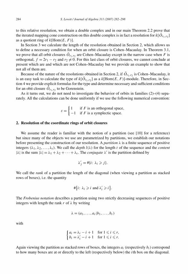
to this relative resolution, we obtain a double complex and in our main Theorem 2.2 prove thatthe iterated mapping cone construction on this double complex is in fact a resolution for k[Or1,r2]as a quotient ring of k[Hom(E,F )].

In Section 3 we calculate the length of the resolution obtained in Section 2, which allows usto define a necessary condition for when an orbit closure is Cohen–Macaulay. In Theorem 3.1,we prove that all orbit closures Or1,r2 are Cohen–Macaulay except in the narrow case when F isorthogonal, f = 2r1 − r2 and r2 �= 0. For this last class of orbit closures, we cannot conclude atpresent which are and which are not Cohen–Macaulay but we provide an example to show thatnot all of them are.

Because of the nature of the resolutions obtained in Section 2, if Or1,r2 is Cohen–Macaulay, itis an easy task to calculate the type of k[Or1,r2] as a k[Hom(E,F )]-module. Therefore, in Sec-tion 4 we provide explicit formulas for the type and determine necessary and sufficient conditionsfor an obit closure Or1,r2 to be Gorenstein.

As it turns out, we do not need to investigate the behavior of orbits in families (2)–(4) sepa-rately. All the calculations can be done uniformly if we use the following numerical convention:

ε ={

1 if F is an orthogonal space,−1 if F is a symplectic space.

2. Resolution of the coordinate rings of orbit closures

We assume the reader is familiar with the notion of a partition (see [10] for a reference)but since many of the objects we use are parametrized by partitions, we establish our notationsbefore presenting the construction of our resolution. A partition λ is a finite sequence of positiveintegers (λ1, λ2, . . . , λt ). We call the depth l(λ) for the length t of the sequence and the content|λ| is the sum |λ| = λ1 + λ2 + · · · + λt . The conjugate λ′ is the partition defined by

λ′j = #{i: λi � j}.

We call the rank of a partition the length of the diagonal (when viewing a partition as stackedrows of boxes), i.e. the quantity

#{i: λi � i and λ′

i � i}.

The Frobenius notation describes a partition using two strictly decreasing sequences of positiveintegers with length the rank r of λ by writing

λ = (a1, . . . , ar |b1, . . . , br )

with {ai = λi − i + 1 for 1 � i � r,

bi = λ′i − i + 1 for 1 � i � r.

Again viewing the partition as stacked rows of boxes, the integers ai (respectively bi ) correspondto how many boxes are at or directly to the left (respectively below) the ith box on the diagonal.


Before beginning the construction, we remind the reader that k[Hom(E,F )] is isomorphic asa k-algebra to Sym(E ⊗ F ∗). Furthermore, since F ∼= F ∗ via the non-degenerate bilinear form〈·,·〉 as pointed out in the introduction, we will identify k[Hom(E,F )] with Sym(E ⊗ F).

As stated in the introduction, our idea for the construction of resolutions of k[Or1,r2] is tobegin with a relative version of the resolution for the coordinate rings of the varieties Oe,r2 overthe Grassmannian Ge−r1(E). Letting Q be the tautological quotient bundle over Ge−r1(E), wewill create a resolution of Sym(Q⊗ F)-modules of a particular ideal sheaf I that corresponds tocertain symmetric or anti-symmetric maps of rank r2 in Hom(Q,Q). Applying the global sectionfunctor Γ (Ge−r1(E),−) to our resolution for I leads to a complex of Sym(E⊗F)-modules fromwhich we produce a resolution for k[Or1,r2] as a quotient ring of k[Hom(E,F )].

To carry out our approach, we need to possess resolutions for the coordinate rings of symmet-ric or anti-symmetric matrices with specified rank. Józefiak, Pragacz and Weyman thoroughlystudied such resolutions in [4] and we borrow their results. For completeness, provide a con-densed description of the terms in the resolution, using a different though equivalent formulationthat will mesh more easily with the results of this paper.

For the variety of anti-symmetric matrices of a specified rank, we remark first that the rankmust be even. The authors in [4] set G = kn, X = Altn(k) the affine space of anti-symmetricmatrices, and Y2p the variety of all matrices of rank at most 2p. The ith component of a minimalfree resolution of k[Y2p] over A = k[X] is equal to

⊕ds(λ)=i

KλG ⊗ A(−|λ|) (3)

where writing the partition λ = (a1, . . . , at |b1, . . . , bt ) in Frobenius notation, λ satisfies bi =ai + 2p + 1 and ds(λ) = ∑t

i=1 ai .For symmetric matrices, in [4] the authors set G = kn, X = Symn(k) the affine space of

symmetric matrices, and Yr is the variety of all matrices of rank at most r . They construct aminimal free resolution of k[Yr ] over A = k[X] whose ith component is equal to⊕

do(λ)=i

KλG ⊗ A(−|λ|) (4)

where writing the partition λ = (a1, . . . , at |b1, . . . , bt ) in Frobenius notation, λ satisfies bi =ai + r − 1, t is even and do(λ) = ∑t

i=1(ai − 1).We are now in a position to present our resolution of k[Or1,r2 ] for any Or1,r2 , an orthogo-

nal or symplectic analogue of a determinantal ideal. However, we first remind the reader of aproposition in homological algebra that plays a central role in our construction.

Proposition 2.1. Let R be a ring. Consider a finite acyclic complex C• of R-modules

0 −→ Cs∂s−→ Cs−1 −→ · · · −→ C1

∂1−→ C0 −→ 0.

Suppose also that for each 0 � i � s we have finite projective resolutions P(i)• −→ Ci −→ 0.

Then there exists a finite projective resolution

L• −→ Coker(∂1) −→ 0 such that Li =⊕

j+k=i

P(j)k .


Proof. This proposition merely describes a standard iterated mapping cone construction so weleave it to the reader as an exercise in homological algebra. (See [2] for a reference.) �

With the iterated mapping cone construction at our disposal, we now present our construc-tion of a resolution of k[Or1,r2] as a module over k[Hom(E,F )]. Let Ge−r1(E) be the Grass-mannian of (e − r1)-dimensional subspaces in E. We have a sequence of tautological bundlesover Ge−r1(E):

0 −→R −→ Ge−r1(E) × E −→Q−→ 0.

Over Ge−r1(E) define the sheaf of algebras A = Sym(Q ⊗ F). Let I be the sheaf of ideals thatcorresponds to injective morphisms φ :Q → F such that rankφ�φ � r2 and consider a minimalfree resolution of A/I:

0 −→Fm −→ · · · −→F2 −→F1 −→ A −→ 0. (5)

Let Γ be the functor of sections over Ge−r1(E). Calling F0 = A for consistency, we obtain thecomplex:

0 −→ Γ (Fm) −→ · · · −→ Γ (F1) −→ Γ (F0) −→ 0. (6)

Furthermore, by Proposition 5.6.1 in [11] we know that (6) is an acyclic complex and hencesatisfies the hypotheses of Proposition 2.1.

From formulas (3) and (4) we can calculate the terms Fm as follows. Let P(a, l) be the set ofpartitions λ contained in the a × (a − l)-rectangle such that if

λ = (a1, . . . , ar |b1, . . . , br )

in Frobenius notation, then bi = ai + l for all 1 � i � r . Let P(a, l)even be the partitions of P(a, l)

with even rank r . Define also the functions

ds(λ) =r∑

i=1

ai and do(λ) =r∑

i=1

(ai − 1)

and the sheaves

Mλ = KλQ⊗ A(−|λ|) with global sections Mλ = Γ (Mλ).

Then the relative version of (3) and (4) over the Grassmannian gives

Fj ={⊕

λ: do(λ)=j Mλ if F is orthogonal,⊕λ: ds(λ)=j Mλ if F is symplectic

and

Γ (Fj ) ={⊕

λ: do(λ)=j Mλ if F is orthogonal,⊕Mλ if F is symplectic
λ: ds(λ)=j


where the summations are taken over λ ∈ P(r1, r2 − ε)even if F is orthogonal and over λ ∈P(r1, r2 − ε) if F is symplectic. Furthermore, we know from [4] that the length of the resolu-tion (5) is

m = (r1 − r2)(r1 − r2 + ε)

2.

We now need to find resolutions for the A-modules Γ (Fj ). We use what is generically calledthe geometric technique and refer the reader to [11, Chapter 5] for a thorough presentation of thetechnique. Using the geometric technique with the bundle ξ = R ⊗ F , we will prove below inLemma 2.3 that the complex F•(Mλ) is an augmented resolution of Mλ as an A-module, whereA = k[Hom(E,F )]. Consequently, we obtain the diagram of A-modules

0 0 0

0 Γ (Fm) · · · Γ (F1) Γ (F0) 0

⊕m F•(Mλ)

⊕1 F•(Mλ)

⊕0 F•(Mλ)

(7)

where the row across the top is a complex, the columns are augmented resolutions and⊕j F•(Mλ) indicates that the direct sum of complexes is taken over all λ in P(r1, r2 − ε)even

(respectively P(r1, r2 − ε)) such that do(λ) = j (respectively ds(λ) = j ). We can therefore useProposition 2.1 to get a non-minimal resolution of the cokernel of the top row, with the termscoming from the other rows in diagram (7).

For each λ ∈ P(r1, r2 − ε), we need to study the complex F•(Mλ) with ξ = R ⊗ F . Weare interested in the length of the complex F•(Mλ) and whether any terms appear in negativedegrees.

By Theorem 5.1.2 in [11], if we set A = k[Hom(E,F )] ∼= Sym(E ⊗ F), then

Fi(Mλ) =⊕j�0

Hj

(Ge−r1(E),

i+j∧(R⊗ F) ⊗ KλQ

)⊗k A(−i − j) (8)

=⊕j�0

⊕μ: |μ|=i+j

Kμ′F ⊗ Hj(Ge−r1(E),Vλ,μ

) ⊗k A(−i − j) (9)

where Vλ,μ is the bundle Vλ,μ = KλQ⊗ KμR over the Grassmannian Ge−r1(E). Consequently,in order to study the terms of the complex F•(Mλ), we must calculate the cohomology groups

Hj(Ge−r1(E),Vλ,μ

)where λ ∈ P(r1, r2 − ε) if F is symplectic, λ ∈ P(r1, r2 − ε)even if F is orthogonal, and μ is inthe rectangle of dimensions (e − r1) × f .

With λ fixed, by Bott’s Theorem (see [11, Theorem 4.1.8] for a reference), two cases mayoccur:


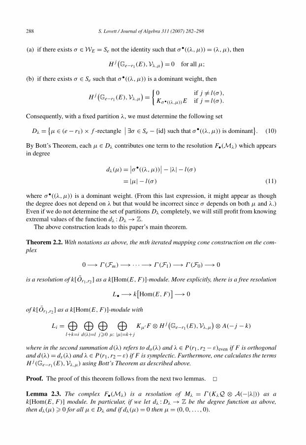
(a) if there exists σ ∈ WE = Se not the identity such that σ •((λ,μ)) = (λ,μ), then


) = 0 for all μ;(b) if there exists σ ∈ Se such that σ •((λ,μ)) is a dominant weight, then


) ={

0 if j �= l(σ ),

Kσ •((λ,μ))E if j = l(σ ).

Consequently, with a fixed partition λ, we must determine the following set

Dλ = {μ ∈ (e − r1) × f -rectangle

∣∣ ∃σ ∈ Se − {id} such that σ •((λ,μ)) is dominant}. (10)

By Bott’s Theorem, each μ ∈ Dλ contributes one term to the resolution F•(Mλ) which appearsin degree

dλ(μ) = ∣∣σ •((λ,μ))∣∣ − |λ| − l(σ )

= |μ| − l(σ ) (11)

where σ •((λ,μ)) is a dominant weight. (From this last expression, it might appear as thoughthe degree does not depend on λ but that would be incorrect since σ depends on both μ and λ.)Even if we do not determine the set of partitions Dλ completely, we will still profit from knowingextremal values of the function dλ :Dλ → Z.

The above construction leads to this paper’s main theorem.

Theorem 2.2. With notations as above, the mth iterated mapping cone construction on the com-plex

0 −→ Γ (Fm) −→ · · · −→ Γ (F1) −→ Γ (F0) −→ 0

is a resolution of k[Or1,r2 ] as a k[Hom(E,F )]-module. More explicitly, there is a free resolution

L• −→ k[Hom(E,F )

] −→ 0

of k[Or1,r2 ] as a k[Hom(E,F )]-module with

Li =⊕

l+k=i

⊕d(λ)=l

⊕j�0

⊕μ: |μ|=k+j

Kμ′F ⊗ Hj(Ge−r1(E),Vλ,μ

) ⊗ A(−j − k)

where in the second summation d(λ) refers to do(λ) and λ ∈ P(r1, r2 − ε)even if F is orthogonaland d(λ) = ds(λ) and λ ∈ P(r1, r2 −ε) if F is symplectic. Furthermore, one calculates the termsHj(Ge−r1(E),Vλ,μ) using Bott’s Theorem as described above.

Proof. The proof of this theorem follows from the next two lemmas. �Lemma 2.3. The complex F•(Mλ) is a resolution of Mλ = Γ (KλQ ⊗ A(−|λ|)) as ak[Hom(E,F )] module. In particular, if we let dλ :Dλ → Z be the degree function as above,then dλ(μ) � 0 for all μ ∈ Dλ and if dλ(μ) = 0 then μ = (0,0, . . . ,0).


Proof. Consider the determinantal variety Y = {φ ∈ Hom(E,F ): rankφ � r1} along with oneof its standard desingularizations

Z = {(φ,R) ∈ Hom(E,F ) × Ge−r1(E): φ|R = 0

}.

Over the Grassmannian V = Ge−r1(E) one has the tautological sequence of vector bundles

0 −→R −→ E −→Q −→ 0.

We then see that Z is the total space of the vector bundle Q∗ ⊗ F and hence in the setup of thegeometric technique we utilize the bundles

η = Q⊗ F ∗,

ξ = R⊗ F ∗.

We employ the set up of [11, Theorem 5.1.2] with the diagram

Z

q ′

Ge−r1(E) × Hom(E,F )

q

Y Hom(E,F ).

We deduce that

H−i

(F•(KλQ)

) = Hi(Ge−r1(E),KλQ⊗ Sym(Q⊗ F)

).

However, by the straightening rule

Symm(Q⊗ F) =⊕

μ: |μ|=m

KμQ⊗ KμF

and Littlewood–Richardson rule, it is not hard to show that

Hi(Ge−r1(E),KλQ⊗ Sym(Q⊗ F)

) ={

KλE if i = 0,

0 if i > 0.

Therefore, the complex F•(Mλ) is in fact a resolution of Mλ as a k[Hom(E,F )] module.The rest of the lemma follows immediately. �

Lemma 2.4. Consider the diagram in Eq. (7). Set A = k[Hom(E,F )]. We have the followingequality of A-modules:

Coker(Γ (F1) → Γ (F0)

) = k[Or1,r2].


Proof. Let us begin by determining the first few terms that resolve M = Coker(Γ (F1) →Γ (F0)). From the iterated mapping cone construction we form a resolution of M which wecall L•. We can easily obtain the terms L0 and L1 from our construction and Proposition 2.1.

L0 = Γ (F0) where F0 = A = Sym(Q⊗F). Thus by Bott’s Theorem over the Grassmannian,whether F is orthogonal or symplectic, we obtain L0 = A = k[Hom(E,F )].

For L1, we recall first that by Proposition 2.1 that L1 = Γ (F1) ⊕ P(0)1 where P

(0)• → Γ (F0)

is an augmented resolution of Γ (F0) as an A module. We notice first that

F1 ={

K(1r2+2)Q⊗ A(−r2 − 2) if F is symplectic,

K(2r2+1)Q⊗ A(−2r2 − 2) if F is orthogonal

and consequently that

Γ (F1) ={∧r2+2

E ⊗ A(−r2 − 2) if F is symplectic,

K(2r2+1)E ⊗ A(−2r2 − 2) if F is orthogonal.

As for calculating P(0)1 , we use formula (9) with λ = 0. We can rewrite (9) in this case as

follows:

P(0)1 =

⊕μ: |μ|�1

Kμ′F ⊗ H |μ|−1(Ge−r1(E),V(0r1 ,μ)

) ⊗ A(|μ|).

If there exists a permutation in the Weyl group of W = Se that sends (0r1 ,μ) to a dominantweight via the dotted action, we call this permutation σμ. By Bott’s Theorem over the usualGrassmannian, if σμ exists for some μ then H |μ|−1(Ge−r1(E),V(0r1 ,μ)) �= 0 only if l(σμ) =|μ| − 1. It is a simple exercise to see that only the partition μ = (r1 + 1,0, . . . ,0) satisfies thisrequirement and that

H |μ|−1(Ge−r1(E),V(0r1 ,μ)

) =r1+1∧

E.

Consequently, we deduce that

L1 ={∧r2+2

E ⊗ A(−r2 − 2) ⊕ ∧r1+1E ⊗ ∧r1+1

F ⊗ A(−r1 − 1) if F is symplectic,

K(2r2+1)E ⊗ A(−2r2 − 2) ⊕ ∧r1+1E ⊗ ∧r1+1

F ⊗ A(−r1 − 1) if F is orthogonal.

The results from [4] and known results from resolutions of determinantal varieties, we identifyIm(L1 → L0) with an ideal I ⊂ A generated by (r2 + 1)-minors of symmetric matrices E → E∗if F is orthogonal (respectively (r2 + 2)-pfaffians on anti-symmetric matrices E → E∗ if F issymplectic) and (r1 + 1)-minors of maps in Hom(E,F ).

In order to finish proving the lemma, we must show that the ideal I is radical, whereCoker(L1 → L0) = A/I . Let us suppose that

√I �= I . Notice that I is equivariant with respect

to the group GL(E) × O(F) (respectively GL(E) × Sp(F )) and hence so is√

I . Let V be anirreducible representation of GL(E) × O(F) (respectively GL(E) × Sp(F )) in

√I but not in I .

Then V is contained in ⊕KλE ⊗ KλF

λ: |λ|�r1


because otherwise V would be contained in the ideal generated by (r1 + 1)-minors of maps inHom(E,F ). But this means that the highest weight vector of V already occurs in Sym(E′ ⊗ F)

where dimE′ = r1. In other words, it is enough to show that the ideal I is reduced in the casewhere dimE = r1. However, this follows as a consequence of the main results in [4] wherethe authors calculate resolutions of the coordinate rings of the space of symmetric (respectivelyanti-symmetric) matrices of rank r2. The authors’ resolutions are precisely

0 −→ Γ (Fm) −→ · · · −→ Γ (F1) −→ Γ (F0) −→ 0

when we assume that dimE = r1. Therefore, the ideal I is radical and the lemma follows. �3. Which orbit closures are Cohen–Macaulay?

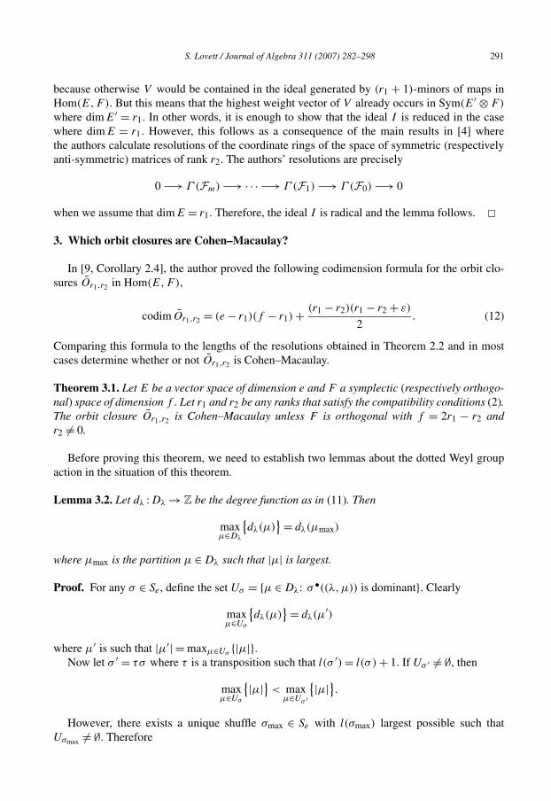
In [9, Corollary 2.4], the author proved the following codimension formula for the orbit clo-sures Or1,r2 in Hom(E,F ),

codim Or1,r2 = (e − r1)(f − r1) + (r1 − r2)(r1 − r2 + ε)

2. (12)

Comparing this formula to the lengths of the resolutions obtained in Theorem 2.2 and in mostcases determine whether or not Or1,r2 is Cohen–Macaulay.

Theorem 3.1. Let E be a vector space of dimension e and F a symplectic (respectively orthogo-nal) space of dimension f . Let r1 and r2 be any ranks that satisfy the compatibility conditions (2).The orbit closure Or1,r2 is Cohen–Macaulay unless F is orthogonal with f = 2r1 − r2 andr2 �= 0.

Before proving this theorem, we need to establish two lemmas about the dotted Weyl groupaction in the situation of this theorem.

Lemma 3.2. Let dλ :Dλ → Z be the degree function as in (11). Then

maxμ∈Dλ

{dλ(μ)

} = dλ(μmax)

where μmax is the partition μ ∈ Dλ such that |μ| is largest.

Proof. For any σ ∈ Se, define the set Uσ = {μ ∈ Dλ: σ •((λ,μ)) is dominant}. Clearly

maxμ∈Uσ

{dλ(μ)

} = dλ(μ′)

where μ′ is such that |μ′| = maxμ∈Uσ {|μ|}.Now let σ ′ = τσ where τ is a transposition such that l(σ ′) = l(σ ) + 1. If Uσ ′ �= ∅, then

maxμ∈Uσ

{|μ|} < maxμ∈Uσ ′

{|μ|}.However, there exists a unique shuffle σmax ∈ Se with l(σmax) largest possible such that

Uσmax �= ∅. Therefore


maxμ∈Dλ

{dλ(μ)

} = dλ(μ′) where μ′ is such that |μ′| = max

μ∈Uσmax

{|μ|}= dλ(μmax) where μmax is such that |μmax| = max

μ∈Dλ

{|μ|}. �

Lemma 3.3. Set A = k[Hom(E,F )]. Let λ be a partition in the rectangle ((r1 − r2 + ε)r1),and let us consider Mλ = Γ (KλQ⊗ A(−|λ|)) as an A-module. One of the following two casesoccurs:

(a) If f − λ1 − r1 � 0, then the projective dimension of Mλ is

pdA(Mλ) = (e − r1)(f − r1).

(b) If f − λ1 − r1 = −1, then the projective dimension of Mλ is

pdA(Mλ) = (e − r1)(f − r1 + 1).

Furthermore, the second case only occurs when ε = 1 (i.e. in the orthogonal case), f = 2r1 − r2

and λ1 = r1 − r2 + ε.

Proof. The technique of the proof is to refer to Lemma 3.2 and find μmax, the largest μ ∈ Dλ

such that there exists a σ ∈ Se such that σ •((λ,μ)) is a dominant weight. In particular,

pdA(Mλ) = dλ(μmax) = |μmax| − l(σ ).

Let 1 � i1 < i2 < · · · < ik = r1 be the indices where λ has jumps. More precisely, we definethe increasing sequence 1 � i1 < i2 < · · · < ik = r1 by the conditions that for all 1 � l � k andall il−1 < i′ � il ,

λi′ = λil and λil > λil+1.

Set n = max{0, f − λ1 − r1}. We remark that since λ is in the rectangle ((r1 − r2 + ε)r1) thecompatibility conditions (2) indicate that n �= f − λ1 − r1 only when f − λ1 − r1 = −1 whichonly occurs when f = 2r1 − r2, ε = 1 and λ1 = r1 − r2 + ε.

We construct the partition μ = μmax by looking at the jumps in λ. The dotted action of a Weylelement will allow up to n entries of μ to get shifted to the left of all entries of λ. At each jump,one can insert at most λil − λil+1 entries of μ. Consequently, we obtain μ by

1 � i � n, μi = f,

n < i � n + λi1 − λi2, λi1 + n = μi − (r1 − i1),

n + λi1 − λi2 < i � n + λi1 − λi3, λi2 + n + λi1 − λi2 = μi − (r1 − i2),

n + λi1 − λi3 < i � n + λi1 − λi4, λi3 + n + λi1 − λi3 = μi − (r1 − i3),...

...


Remarking that λi1 = λ1 we rewrite this as

1 � i � n, μi = f,

n < i � n + λi1 − λi2, μi = λ1 + n + r1 − i1,

n + λi1 − λi2 < i � n + λi1 − λi3, μi = λ1 + n + r1 − i2,

n + λi1 − λi3 < i � n + λi1 − λi4, μi = λ1 + n + r1 − i3,...

...

But we must have i � |μ| = e − r1 so these intervals over which we have defined μ stop at theindex j where

n + λ1 − λij < e − r1 � n + λ1 − λij+1 . (13)

Thus for the indices n + λ1 − λij < i � e − r1 we set μi = λ1 + n + r1 − ij .Therefore we obtain

|μmax| = f n + (λi1 − λi2)(λ1 + n + r1 − i1) + (λi2 − λi3)(λ1 + n + r1 − i2) + · · ·+ (λij−1 − λij )(λ1 + n + r1 − ij−1) + (e − r1 − n − λ1 + λij )(λ1 + n + r1 − ij ).

Furthermore, it is not too hard to see that

l(σ ) =∑i,j

#{(i, j): λi + e − i < μj + e − r1 − j

}

and by our construction of μ this is equal to

l(σ ) = nr1 + (λi1 − λi2)(r1 − i1) + (λi2 − λi3)(r1 − i2) + · · ·+ (λij−1 − λij )(r1 − ij−1) + (e − r1 − n − λ1 + λij )(r1 − ij ).

Consequently, we obtain

dλ(μmax) = |μmax| − l(σ )

= n(f − r1) + (λ1 − λij )(λ1 + n) + (e − r1 − n − λ1 + λij )(λ1 + n) (14)

= n(f − r1) + (e − r1 − n)(λ1 + n). (15)

A perhaps surprising remark to this equality is that dλ(μmax) does not depend on the jumps in λ

or the indices il .At this point, we consider two cases depending on the value of n.

Case 1. Suppose that f − λ1 − r1 � 0 which is false only when f = 2r1 − r2, ε = 1 and λ1 =r1 − r2 + 1. In this case, n = f − λ1 − r1. When we replace n = f − λ1 − r1 in Eq. (15), weobtain the following expected result after a few manipulations:

dλ(μmax) = (e − r1)(f − r1).


Case 2. Suppose that f − λ1 − r1 = −1 which is true only when f = 2r1 − r2, ε = 1 andλ1 = r1 − r2 + 1. In this case, n = 0 = f − λ1 − r1 + 1. When we replace n = f − λ1 − r1 + 1in Eq. (15), we obtain the following expression after a few manipulations:

dλ(μmax) = (f − λ1 − r1 + 1)(f − r1) + (e − f + λ1 − 1)(f − r1 + 1)

= (e − r1)(f − r1 + 1). �Proof of Theorem 3.1. Suppose first that F is orthogonal (i.e. ε = 1) and f = 2r1 − r2. The-orems 4.9 and 4.10 in [9] establish that given this assumption Or1,r2 is Cohen–Macaulay whenr2 = 0. Notice that if we assume dimF = 2r1 − r2, r2 = 0 implies that F is even dimensional.

Suppose now that ε �= 1 or f > 2r1 − r2. By Proposition 3.3, the resolution L• created by theiterated mapping cone construction has length

(e − r1)(f − r1) + (r1 − r2)(r1 − r2 + ε)

2

which according to (12) is precisely the codimension of Or1,r2 .Even though L• is not a minimal resolution, a minimal resolution of k[Or1,r2 ] must have

length less than or equal to (e − r1)(f − r1) + (r1 − r2)(r1 − r2 + ε)/2. However, by standardmethods of algebraic geometry, a minimal resolution cannot be shorter than codim Or1,r2 andhence it must have this length. This proves that Or1,r2 is Cohen–Macaulay. �

Theorem 3.1 singles out the rather narrow case of orbits Or1,r2 that satisfy F orthogonal,f = 2r1 − r2 and r2 �= 0. Currently, in this article, we are not able to establish which of theseorbits are not Cohen–Macaulay. However, we cannot hope that all orbits are Cohen–Macaulayand that our methods just are not subtle enough to prove them so because, as the followingexample shows that some orbits in this narrow case are not Cohen–Macaulay.

Example 3.4. Let us consider F orthogonal, dimE = 4, dimF = 5, r1 = 3 and r2 = 1. Thecodimension of the orbit closure if given by

codim Or1,r2 = (e − r1)(f − r1) + (r1 − r2)(r1 − r2 + 1)

2= 5.

On the other hand, the iterated mapping cone construction leads to the following resolution ofthe coordinate ring k[Or1,r2] as an A-modules, where A = k[Hom(E,F )].

0

↓

K(34)E ⊗4∧

F ⊗ A(−12)

↓

K(32,22)E ⊗2∧

F ⊗ A(−10) ⊕ K(33,2)E ⊗5∧

F ⊗ A(−11)

↓


K(32,2,1)E ⊗ F ⊗ A(−9) ⊕ K(3,23)E ⊗3∧

F ⊗ A(−9)

↓

K(32,2)E ⊗ A(−8) ⊕ K(3,2,12)E ⊗ F ⊗ A(−7) ⊕ K(23,1)E ⊗3∧

F ⊗ A(−7)

↓

K(3,2,1)E ⊗ A(−6) ⊕ K(22,12)E ⊗ F ⊗ A(−6) ⊕ K(2,13)E ⊗5∧

F ⊗ A(−5)

↓

K(22)E ⊗ A(−4) ⊕4∧

E ⊗4∧

F ⊗ A(−4)

↓A

↓0

One can tell that this resolution is minimal from the fact that terms in neighboring homologicaldegrees occur in different homogeneous degrees. However, since it has length 6 and in particularis strictly greater than codim Or1,r2 , the orbit closure is not Cohen–Macaulay.

4. Calculations of type

As an application of the techniques presented in the above subsection, we propose to calcu-late the type of the orbit closure Or1,r2 which is an important algebraic invariant. We state thedefinition given in [1].

Definition 4.1. Let (R,m, k) be a local Noetherian ring and M a finite R-module of depth t . Thenumber r(M) = dimk ExttR(k,M) is called the type of M .

We work in the ring A = k[Hom(E,F )] and study the module M = k[Or1,r2 ]. For everymaximal ideal m ∈ SuppM , Am/mm = k and depthMm is unchanged as is dimk ExttAm

(k,Mm).

We also call this common number the type of M = k[Or1,r2] and write it r(Or1,r2). We can easilyshow that r(Or1,r2) is the dimension of the top free module in a minimal resolution of k[Or1,r2]as an A module.

In the previous subsection where we constructed the free resolution L• of k[Or1,r2] as anA-module, we did not obtain a minimal resolution. However, in every case except when F isorthogonal with f = 2r1 − r2, we obtained a resolution of depth equal to codim Or1,r2 with asingle term of the form KλE ⊗ KμF ⊗ A(−|λ|) in the top term. Consequently, in a minimalresolution of k[Or1,r2 ], the term of maximal degree is equal to the term of maximal degree weobtained by our iterated mapping cone construction. Let us prosaically call this term Top(Or1,r2).Therefore we can calculate r(Or1,r2) = dim Top(Or1,r2) fairly easily.


Proposition 4.2. Let E we a vector space of dimension e and F be a symplectic space of dimen-sion f . Consider the orbit closure Or1,r2 . One of the three following cases occurs:

(a) If f − e − r1 + r2 + 1 < 0 then

r(Or1,r2) =∏

1�i�f −r11�j�r1

e − r2 + j − i − 1

f − r1 + j − i.

(b) If f − e − r1 + r2 + 1 = 0 then

r(Or1,r2) = 1.

(c) If f − e − r1 + r2 + 1 > 0 then

r(Or1,r2) =∏

1�i�e−r11�j�r1

f − 2r1 + r2 + j − i + 1

e − r1 + j − i.

Proof. Note that since F is symplectic, we have ε = −1.We determine Top(Or1,r2) as Fmax(KλmaxQ) in the same way we determined projective

dimension of F•(KλmaxQ) in Proposition 3.3. We know that when F is symplectic λmax =((r1 − r2 − 1)r1). We now need to calculate the partition μ such that

Fmax(KλmaxQ) = Hl(σ)(Ge−r1(E),Vλ,μ

) ⊗ Kμ′F.

In order to do so, we must consider three separate cases.

Case 1. f − e − r1 + r2 + 1 < 0.

Following the calculations in Proposition 3.3, we obtain

μ = (f (f −2r1+r2+1), (f − r1)

(e−f +r1−r2−1)).

Furthermore, a simple check yields σ •((λ,μ)) = ((f − r1)e) which leads to

r(Or1,r2) = dimK(f −r1)eE ⊗ Kμ′F = dimKμ′F

where μ′ = ((e − r1)(f −r1), (f − 2r1 + r2 + 1)r1). Recall the well-known formula (see [3, The-

orem 6.3]) for the dimension of a Weyl module of a vector space E:

dimKλE =∏

1�i<j�dimE

λi − λj + j − i

j − i. (16)

Applying this to Kμ′F and ignoring all factors that are equal to 1 we obtain precisely the formulain part (a).

Case 2. f − e − r1 + r2 + 1 = 0.


We note in this case that the method in part (a) works equally well but that μ′ = ((e − r1)f )

so dimKμ′F = 1.

Case 3. f − e − r1 + r2 + 1 > 0.

Following the calculations in Proposition 3.3, we obtain μ = (f (e−r1)) and σ •((λ,μ)) =((f −r1)

(e−r1), (e−r1 −1)r1). Again after some rearranging and cancellation, using formula (16)we deduce the expression in the statement of the proposition. �

As often seems the case, calculations for when F is orthogonal pose a few more difficultiesthan for when F is symplectic. First of all, the iterated mapping cone construction does not givesus a free resolution of the proper depth if f = 2r1 − r2 and hence we cannot thereby determineTop(Or1,r2).

Secondly, all the partitions λ appearing in the resolution (7) have even rank. Thus λmax =((r1 − r2 + 1)r1) only when min(r1, r1 − r2 + 1) is even. If min(r1, r1 − r2 + 1) is odd, then

λmax = ((r1 − r2 + 1)(r1−r2), (r1 − r2)

r2).

The method to calculate μ in Proposition 3.3 still applies, but because λmax is not a rectangle, oneis led to consider more options than in Proposition 4.2. The calculations are not particularly en-lightening so we do not carry them out. Nonetheless, we can conclude with a simple propositionthat states which coordinate rings k[Or1,r2] are Gorenstein.

Proposition 4.3. Let E be a vector space of dimension e and F either a symplectic or orthogonalspace of dimension f .

(a) If F is symplectic, then k[Or1,r2 ] is Gorenstein if and only if f − e − r1 + r2 = −1.(b) If F is orthogonal with f > 2r1 − r2, then k[Or1,r2] is Gorenstein if and only if f − e − r1 +

r2 = 1 and min(r1, r1 − r2 + 1) is even.

Proof. We recall that a Noetherian ring is Gorenstein if it is Cohen–Macaulay and of type 1.(See [1, Theorem 3.2.10].)

Part (a) follows almost immediately from Proposition 4.2. Part (b) of Proposition 4.2 estab-lishes the direction (⇐). Furthermore, we can easily rewrite the products in parts (a) and (c) sothat all the terms in the product are greater than 1 and hence produce a type that is greater than 1.This proves the (⇐) direction.

For part (b), let us first assume that f > 2r1 − r2 and hence that the iterated mapping coneconstruction provides a resolution of k[Or1,r2] of length equal to the codimension of Or1,r2 . Ifmin(r1, r1 − r2 + ε) is even then λmax = (r1 − r2 + 1)r1 and we can apply identical methodsas Proposition 4.2 with the only change that ε = 1. On the other hand, if min(r1, r1 − r2 + ε)

is odd, then since λmax is not a rectangle, a quick check of all possibilities shows that μ andσ •((λmax,μ)) cannot both be rectangles and hence r(Or1,r2) > 1. �

We conclude with an example that illustrates Proposition 4.3.

Example 4.4. Let E be a vector space with dimE = 5 and F an orthogonal vector space withdimF = 7. Let us choose rank conditions r1 = 4 and r2 = 3. Since F is orthogonal, ε = 1 and


thus f − e − r1 + r2 − ε = 0. Furthermore, min(r1, r1 − r2 + 1) = 2 is even and f > 2r1 − r2and hence k[Or1,r2] is Gorenstein.

Using Theorem 2.2, then decomposing Schur functors of F into irreducible O(F)-modules(see [6]), we can find the minimal resolution of k[Or1,r2]. It is as follows:

0

↓K(35)E ⊗ A(−15)

↓K(25)E ⊗ V(1,1)F ⊗ A(−10) ⊕ K(3,14)E ⊗ A(−7)

↓K(24,1)E ⊗ F ⊗ A(−9) ⊕ K(2,14)E ⊗ F ⊗ A(−6)

↓K(24)E ⊗ A(−8) ⊕ K(15)E ⊗ V(1,1)F ⊗ A(−5)

↓A

↓0

where V(1,1)F is irreducible representation of so(F ) of highest weight (1,1). (We used resultsin [6] to pass between Schur functors of F and irreducible representations of so(F ).)

As the subject of a future article, the author plans to study where these examples of Gorensteinorbit closures of codimension 4 fit into the classifications done by Kustin and Miller in [7].

References

[1] W. Bruns, J. Herzog, Cohen–Macaulay Rings, Cambridge Stud. Adv. Math., vol. 39, Cambridge Univ. Press, Cam-bridge, 1993.

[2] D. Eisenbud, Commutative Algebra with a View Toward Algebraic Geometry, Grad. Texts in Math., vol. 150,Springer-Verlag, New York, 1995.

[3] W. Fulton, J. Harris, Representation Theory, Grad. Texts in Math., vol. 129, Springer-Verlag, New York, 1991.[4] T. Józefiak, P. Pragacz, J. Weyman, Resolutions of determinantal varieties and tensor complexes associated with

symmetric and antisymmetric matrices, Astérisque 87–88 (1981) 109–189.[5] V.G. Kac, Some remarks on nilpotent orbits, J. Algebra 64 (1980) 190–213.[6] K. Koike, I. Terada, Young diagrammatic methods for the representation theory of the classical groups of type Bn ,

Cn, Dn , J. Algebra 107 (1987) 466–511.[7] A. Kustin, M. Miller, Classification of the tor-algebras of codimension four Gorenstein local rings, Math. Z. 190

(1985) 341–355.[8] A. Lascoux, Syzygies des variétés déterminantales, Adv. Math. 30 (3) (1978) 202–237 (in French).[9] S.T. Lovett, Orthogonal and symplectic analogues of determinantal ideals, J. Algebra 291 (2005) 416–456.

[10] I.G. Macdonald, Symmetric Functions and Hall Polynomials, Oxford Univ. Press, Oxford, 1999.[11] J.M. Weyman, Cohomology of Vector Bundles and Syzygies, Cambridge Tracts in Math., vol. 149, Cambridge

Univ. Press, New York, 2003.

Resolutions of orthogonal and symplectic analogues of determinantal ideals

Documents

Transcript of Resolutions of orthogonal and symplectic analogues of determinantal ideals