Residual welding stresses and distortions - web.alt.uni...
27
Residual welding stresses and distortions _____________________________________________________________________________________ When steel structures are constructed by welding, deformations and welding residual stresses could occur as a result of the high heat input and subsequent cooling (Boley & Weiner 1960). The welding process can create significant locked-in stresses and deformations in fabricated steel structures (Rykalin 1951). The residual stresses and initial imperfections can have an important influence upon the behaviour of the structure under the variable loading (Gurney 1979). It is well known that these initial imperfections due to welding reduce the ultimate strength of the structure. Even though various efforts have been made in the past to express the deflection of panels from experimental aspects and measurements of actual structures, it may be said that there are few investigations from the theoretical point of view. In order to find out a practical estimation method for the welding distortion of a panel, the following analyses have been carried out by Okerblom (1955). To determine the thermal effect on the structure it is advisable to investigate some simple structures (Chang Doo Jang & Seung Il Seo 1995). Finite element calculations can help to determine these residual stresses (Josefson 1993, Wikander et al. 1994). 1.1 Simple examples of thermoelasticity We assume the following: - the coefficient of thermal expansion and the Young modulus are independent from the temperature, - the deflections are in the elastic range, the Hooke-law is valid, - the cross sections of the beam will be planar after deflection, - the cross section is uniform, - the beam is made of one material grade, - the thermal distribution is uniform along the length of the beam and steady state. The change in length ( ) and deflection ( ) of a simply supported beam, as shown in Fig. 1.1 due to linear heat distribution is as follows: ΔL w max The strain in the centre of gravity is ε α α G o es o e e T T T h = = − ( / 1 1 ) Δ e . Here Δ is the temperature difference and T T e e e = - T 1 2 α o is the coefficient of thermal expansion. The change in length ( ΔL ) caused
Transcript of Residual welding stresses and distortions - web.alt.uni...

Residual welding stresses and distortions _____________________________________________________________________________________
When steel structures are constructed by welding, deformations and welding residual stresses could occur
as a result of the high heat input and subsequent cooling (Boley & Weiner 1960). The welding process
can create significant locked-in stresses and deformations in fabricated steel structures (Rykalin 1951).
The residual stresses and initial imperfections can have an important influence upon the behaviour of the
structure under the variable loading (Gurney 1979). It is well known that these initial imperfections due
to welding reduce the ultimate strength of the structure.
Even though various efforts have been made in the past to express the deflection of panels from
experimental aspects and measurements of actual structures, it may be said that there are few
investigations from the theoretical point of view. In order to find out a practical estimation method for the
welding distortion of a panel, the following analyses have been carried out by Okerblom (1955).
To determine the thermal effect on the structure it is advisable to investigate some simple structures
(Chang Doo Jang & Seung Il Seo 1995). Finite element calculations can help to determine these residual
stresses (Josefson 1993, Wikander et al. 1994).
1.1 Simple examples of thermoelasticity
We assume the following:
- the coefficient of thermal expansion and the Young modulus are independent from the
temperature,
- the deflections are in the elastic range, the Hooke-law is valid,
- the cross sections of the beam will be planar after deflection,
- the cross section is uniform,
- the beam is made of one material grade,
- the thermal distribution is uniform along the length of the beam and steady state.
The change in length ( ) and deflection ( ) of a simply supported beam, as shown in Fig. 1.1 due to
linear heat distribution is as follows:
ΔL wmax
The strain in the centre of gravity is ε α αG o es o e eT T T h= = −( /1 1 )Δ e . Here Δ is the
temperature difference and
T Te e e= - T 1 2
α o is the coefficient of thermal expansion. The change in length (ΔL ) caused

by heat expansion is ΔL G= Lε . The heat distribution is non-uniform at the cross section, so a curvature
occurs at the beam. The radius of curvature is ρ o .
Fig. 1.1 Deflections of a beam with linear temperature distribution
The curvature is C Tho
o e= =1ρ
α Δ. There is a relation between radius of curvature, bending moment and
bending stiffness as 1ρ o x
MEI
= . So the curvature can be considered as the effect of a uniform bending
moment across the length as M T EIh
o e x=α Δ .
The rotation of the angle is ϕ( )z MEI
L zx
= −⎛⎝⎜
⎞⎠⎟2
, so the maximum value is ϕ max =CL2
.
The deflection is (w z MEI
Lz zx
( ) = −2
2 ) , so the maximum value is w CLmax =
2
8.
Another problem is, when the thermal distribution is nonlinear as shown in Fig. 1.2. The thermal strain
would be different at different points of cross section if they were independent form each other:
ε α= o eT y( ) . Because they are connected to each other, we assume that the cross section remains planar,
only a linear strain can occur in the cross section. This linear strain is characterized by the strain of the
gravity centre and the curvature of the beam: ε ε= +G Cy . The differences between the theoretical
thermal strain and the linear strain cause the stresses:
σ ε ε α= = + −E E Cy T yG o e{ ( )} (1.1)
There is no external loading on the beam, so the internal stresses caused by thermal difference are in
equilibrium,
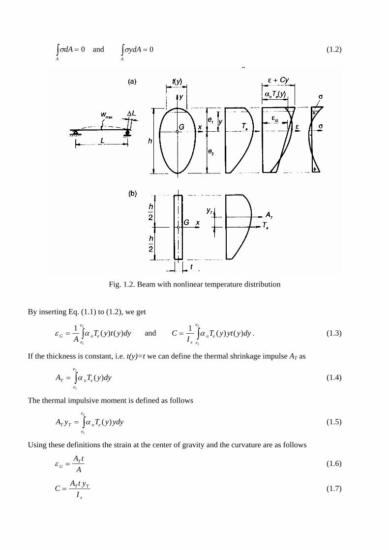
and (1.2) σdAA
=∫ 0 σydAA
=∫ 0
Fig. 1.2. Beam with nonlinear temperature distribution
By inserting Eq. (1.1) to (1.2), we get
ε αG o ee
e
AT y t y dy= ∫
1
1
2
( ) ( ) and CI
T y yt y dyx
o ee
e
= ∫1
1
2
α ( ) ( ) . (1.3)
If the thickness is constant, i.e. t(y)=t we can define the thermal shrinkage impulse AT as
(1.4) A T yT o ee
e
= ∫α ( )1
2
dy
The thermal impulsive moment is defined as follows
(1.5) A y T y ydyT T o ee
e
= ∫α ( )1
2
Using these definitions the strain at the center of gravity and the curvature are as follows
ε GTA tA
= (1.6)
CA t y
IT T
x
= (1.7)

1.2 The Okerblom’s analysis
When a structural section is welded, it undergoes distortion as a result of thermal shrinkage along the axis
of the weld. For example, an edge-welded bar section shortens (ΔL ) and deflects ( ). Experiments
indicate that the Okerblom’s analysis provides excellent prediction for longitudinal deflections caused by
thermal shrinkage along the weld (Okerblom 1955, Okerblom et al 1963).
wmax
The analytical heat-transfer theory of welding was developed by Rykalin (1951). Essentially, Okerblom
utilises the analytical heat-transfer theory of moving heat sources to establish the thermal strain and stress
distributions around the weld. The primary objective of the Okerblom’s analysis is to predict the beam
shrinkage (Δ ) and deflection (w) as shown in Fig. 1.1. The analysis is used to generate a series of
temperature isotherms that are stationary with respect to the heat source (Fig. 1.3).
L
Fig. 1.3 Strain distribution during and after welding

In the Okerblom’s analysis the material is linearly elastic and ideally plastic. The yield stress is constant
till 500 Co, and between 500 and 600 Co it decreases to zero. If the temperature is larger than 600 Co,
there is no measurable stress in material (Fig. 1.4).
Fig. 1.4 The yield stress in the function of the temperature and strain

Fig. 1.5 Distribution of thermal strains during and after welding
The approximation of the Te temperature suggested by Okerblom is as follows
TQ
c t yeT
o
=0 4840
2.ρ
(1.8)
where c0 is the specific heat, ρ is the material density, t is the thickness of the plate.
The thermal impulse can be calculated according to Fig. 1.5. The diagram determined by points 1-10
shows the stress distribution during welding. It can be obtained by projection of points B and C to the line
ε A which occurs due to elastic deformation of the structure during welding. Points B and C are
determined by the line 600o α , so between points 5 and 6 no stresses occur. Points 3-4 and 7-8 are
obtained by the line parallel to line ε A in a distance εy , with projection to this line the points D and E
determined by the line 500o α . It can be seen that plastic strains occur during welding between points 3
and 8. These retrained strains cause residual stresses after cooling.
The residual stress diagram after cooling can be obtained projecting points 3 and 8 onto the basic line 1’-
10’. Considering the elastic deformation during cooling and the line of ′ ≈ε εA A εy , one obtains the

residual stress diagram 1’-3’-F’-G’-8’-10’. The area 3’-F’-G’-8’ characterizes the thermal shrinkage
impulse AT which causes the residual stresses and deformations in the structure.
Since the line parts of 3’-F’ and 8’-G’ are the same as parts 3-F and 8-G, the AT can be calculated by
investigating the area 3-F-G-8 in the diagram drawn for the state during welding.
A b dTQ
c tdTTT o e
o T
o
e
eT
T T
A y
A y
e A y o
e e
= =+
+
= +
=
∫ ααρε ε
ε ε
ε ε α
2 20 4840
1
2 1( )
( )/
.∫ (1.9)
AQ
c tQ
c tTo T
o
o T
o
= =0 4840
20 3355.
ln.α
ραρ
(1.10)
where Q UIv
q AT ow
o w= =η , U arc voltage, I arc current, vw speed of welding, co specific heat, ηo
coefficient of efficiency, q0 is the specific heat for the unit welded joint area (1 mm2), Aw is the welded
joint area.
For a mild or low alloy steels, where α o =12*10-6 [1/Co], coρ = 4.77*10-3 [J/mm3/Co], the thermal
impulse is
. A t QT T [mm ] [J / mm]2 = −0844 10 3. *
Inserting this into Eqs. (1.6) and (1.7), we get the basic Okerblom formulae
ε GTA tA
QA
= = − −0 844 10 3. * T (1.11)
The minus sign means shrinkage.
CA t y
IQ y
IT T
x
T T
x
= = − −0844 10 3. * (1.12)
Note that the distorted form can be determined by view. yT and C have opposite signs (Fig. 1.15).
The elastic strain in the weld can be calculated using the previous two expressions
ε εA G Cy= + T (1.13)
The average width of the plastic tension zone around the weld is
bA
yT
A y
=+ε ε
(1.14)
At the region of weld the residual tensile stress after welding reaches the yield stress (Fig. 1.5). The area
of the plastic zone is
A b tA t
y yT
A y
= =+ε ε
(1.15)
By using Eqs. (1.6), (1.7) and (1.13) one obtains

1 1 2
A AyI Ay
T
x
y
T
= + +t
ε (1.16)
If no crookedness is developed in beam during welding, as for example in the case of a symmetrical weld
arrangement, Eq. (1.16) takes the form
1 1A A Ay
y
T
= +t
ε (1.17)
For steels
1 1 142
A AyI Qy
T
x T
= + +.3 [J, mm] (1.18)
If the structure can be regarded as a very stiff one, when ε A = 0 , area of plastic zone is
1A Ay
y
T
=t
ε (1.19)
For steels
A Qy
T=143.
(1.20)
The equilibrium equation for a section with tension and compression stresses is according to Fig. 1.6
( )b b b fy c y− = yσ (1.21)
Fig. 1.6 Approximate stress distribution for a plate with a single weld at the middle
Using Eq. (1.17) one can compute the residual compressive stress,
σε
α ηρc
T y
y
T o
o w
AA
A tA
EUIE
c v= = =
t f b t
0 3355. o (1.22)

With data , α o =−11 10 6* coρ = ⎡
⎣⎢⎤⎦⎥
−353 10 3. * Jmm C3 o , E = 2.05*105 [MPa], vw is the welding speed,
used by White, the Okerblom formula is
ση
co
w
UIv bt
=0 214.
, (1.23)
White (1977a,b) proposed an approximate formula based on own experiments
ση
co
w
UIv bt
=0 2.
, (1.24)
It can be seen that Okerblom’s formula is in agreement with White’s experimental results.
The formulae above are valid for symmetrically arranged welds yA = 0
QA
T ≤ ⎡⎣⎢
⎤⎦⎥
2 50. Jmm3 , (1.25)
for eccentric welds ( )yA ≠ 0
QA
T ≤ ⎡⎣⎢
⎤⎦⎥
0 63. Jmm3 . (1.26)
For approximate calculations one can use the simple formula
ε yyf
E= (1.27)
where fy is the yield stress of the parent material. The weld metal may have a different yield stress. This
discrepancy arises due to the electrode material. In this case it is important to measure the yield stress of
the weld metal. Using high strength steels, the yield stress of the weld metal can be smaller that of the
parent material. Therefore the residual stresses are relatively smaller, than in the case of mild steel.
For some simple cross sections the residual stress distribution can be seen on Fig. 1.7.

Fig. 1.7 Residual stresses in different cross sections and weld positions
1.3 Multi-pass welding
The basic Okerblom formulae are valid for single pass-welding. For multi-pass welding it is necessary to
modify Eq. (1.10.), because the new weld pass resolves the plastic zone, made by the previous weld pass.
For the value of residual stresses that weld pass is governing, which causes the largest plastic zone.
Introducing a parameter for the correction of thermal shrinkage impulse
A mQ
c tT to T
o
=0 3355. α
ρ (1.28)
where mAAt
yt
y
=1
, (1.29)
Ay1 , Ayt the areas of plastic zone due to single- and multi-pass welding.
For example at a two-pass (equal passes) butt joint mt = 1. For a double fillet weld for thin plates, where
the welds are welded one after the other mt = 12 13. - . . For intermittent fillet welds m LLt
w
u
= , where Lw
and Lu are the distances of the welded and unwelded part at intermittent fillet weld.
White (1977c) suggested to calculate the tendon force from the parameters of that pass, which has the
greatest section area.
The effect of preheating can be taken account with a correction parameter

FT
Fp' ( . )= −111000
(1.30)
where the temperature of preheat is T Co. p > 100
1.4 Effect of initial strains
In the previous calculations it was assumed, that there are no initial strains and stresses in the structure. In
practice there are usually some strains and stresses before welding, or previous welds cause initial strains
and stresses for the next weld(s). Preheating, flame cutting and pre-stressing have the same effect.
The strain diagram is similar to Fig. 1.5 except of the initial tensile strain ε I . Fig. 1.8 shows the strain
distribution during welding and after welding. The final deformations after welding are caused by the
difference of ε εy − I . The effective zone is between ABCD point. The thermal impulse can be computed
as follows:
′ = =+ =
=
∫A b dTQ
c tdTTT o e
o T
o
e
eT
T
I y
y
e I y o
e y
ααρε ε
ε
ε ε α
ε α2 20 4840
1
2 0.
( )/
/
+∫ (1.31)
′ =+
AQ
c tTo T
o
y
y I
0 4840 2.ln
αρ
εε ε
(1.32)
To consider the effect of initial deformation we introduce a modifying parameter ν m , which is the ratio of
the thermal impulse with and without initial strain.
ν
εε ε
εmT
T
I
y I
y
AA
=′
= −
+
≈ −11
21
ln( )
ln (1.33)
The approximate formulae is valid when εε
I
y
≥ 0.

Fig. 1.8 Distribution of thermal strains during and after welding due to initial strains
Fig. 1.9 shows ν m in the function of εε
I
y
. Without initial deformation no modification is necessary, so if
ε I = 0, then ν m =1. If there is a tension in the elastic zone, 0 < <ε εI y 0, then 1> >ν m . If the initial
strain is equal to the yield strain, ε εI y= , ν m = 0 , there is no residual stresses and deformations after
welding. If the initial strain is negative (compression), ε I < 0, ν m > 1, this strain increases the
deformation, but the approximate formula can not be used.
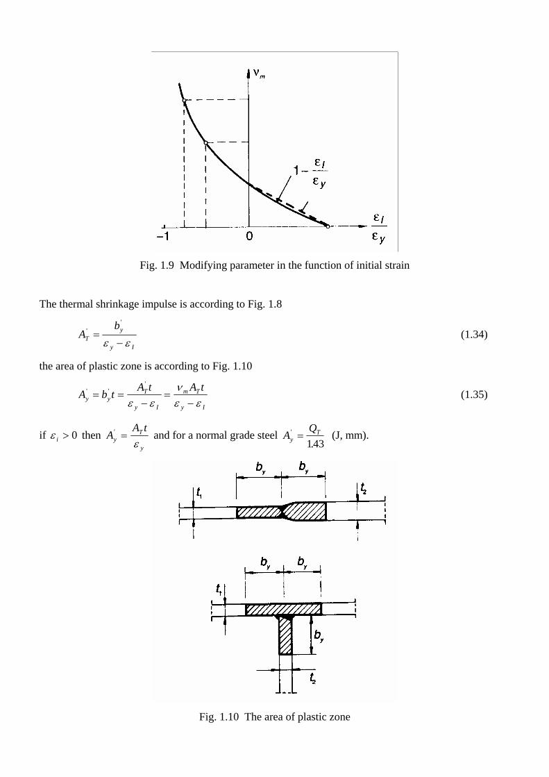
Fig. 1.9 Modifying parameter in the function of initial strain
The thermal shrinkage impulse is according to Fig. 1.8
Ab
Ty
y I
''
=−ε ε
(1.34)
the area of plastic zone is according to Fig. 1.10
A b tA t A t
y yT
y I
m T
y I
' ''
= =−
=−ε ε
νε ε
(1.35)
if ε i > 0 then AA t
yT
y
' =ε
and for a normal grade steel AQ
yT'
.=
143 (J, mm).
Fig. 1.10 The area of plastic zone
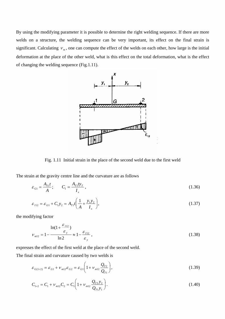
By using the modifying parameter it is possible to deternine the right welding sequence. If there are more
welds on a structure, the welding sequence can be very important, its effect on the final strain is
significant. Calculating ν m , one can compute the effect of the welds on each other, how large is the initial
deformation at the place of the other weld, what is this effect on the total deformation, what is the effect
of changing the welding sequence (Fig.1.11).
Fig. 1.11 Initial strain in the place of the second weld due to the first weld
The strain at the gravity centre line and the curvature are as follows
ε GTA tA1
1= ; CA ty
IT T
x1
1= , (1.36)
ε εI G Tx
C y A tA
y yI12 1 1 2 11 21
= + = +⎛⎝⎜
⎞⎠⎟ , (1.37)
the modifying factor
ν
εε ε
εm
I
y I
y12
12
1211
21= −
+
≈ −
ln( )
ln , (1.38)
expresses the effect of the first weld at the place of the second weld.
The final strain and curvature caused by two welds is
ε ε ν ε ε νG G m G G mT
T
QQ( )1 2 1 12 2 1 12
2
1
1+ = + = +⎛⎝⎜
⎞⎠⎟ , (1.39)
C C C C Q yQ ym m
T
T1 2 1 12 2 1 12
2 2
1 1
1+ = + = +⎛⎝⎜
⎞⎠⎟ν ν . (1.40)

Changing the welding sequence ε G( )2 1+ and can be calculated using Eqs (1.39) and (1.40), changing
the subscripts:
C2 1+
ε ε ν ε ε νG G m G G mT
T
QQ( )2 1 2 21 1 2 21
1
2
1+ = + = +⎛⎝⎜
⎞⎠⎟ , (1.41)
C C C C Q yQ ym m
T
T2 1 2 21 1 2 21
1 1
2 2
1+ = + = +⎛⎝⎜
⎞⎠⎟ν ν . (1.42)
Comparing the two strains and curvatures, the smallest absolute value gives the better welding sequence.
If there are two longitudinal welds in an asymmetric I-beam and the 1st weld is closer to the gravity
center, y y1 < 2 , it means C C1 < 2
1
, so the 2nd weld has greater effect that the 1st one. The modifying
parameter is always less then 1 in this case, 0 < <ν m . The conclusion is, that the closer weld should be
made first, because the final deformation will be less, C C1 2 2 1+ +< .
The maximum deflection caused by welding is
w C Lmax =
2
8, w C L
1 2 1 2
2
8+ += , w C L2 1 2 1
2
8+ += . (1.43)
1.5 The effect of external loading on the welding residual stresses
To investigate the effect of static tension forces on residual stresses, we simplify the distribution of
residual stresses according to Fig. 1.12.
The stresses in the tension field are σ b , in the compression field σ a . If the sum of tension stresses due to
the external force and the residual stress is less than the yield stress, , the resulting
stress on the width part (b) of the plate is , on the width part (a) of the plate .
If the tension stresses due to the external force are larger , in this case on the width part (b)
of the plate , on the width part (a) of the plate
σ σ σe yf< = −'b
e e
y
y
σ σ σb b' = + σ σ σa a
' = +
σ σ' ≤ ≤e f
σ b f'' =
σ σ σ σ σa a ea b
a'' ' '( )= + + −
+22
(1.44)
During unloading, all fibres deform elastically
σ σ σ σ σ σa a e a e y bf ba
''' '' (= − = + − +2
)
e
(1.45)
(1.46) σ σ σ σb b e yf''' ''= − = −

It can be seen, that the residual stresses decrease. If the external force were , then there
no residual stresses remain (Fig. 1.12) and if the material is ideally plastic, then the residual stresses will
cut down to zero but residual deformations will occur.
F f t a by y= +(2 )
Fig. 1.12 Simplified residual stress distribution and the cutting down of initial stresses due to static
loading
1.6 Reduction of residual stresses
There are several ways to reduce the deformation and the residual stresses in the welded structures. They
are as follows:
Reduction techniques in the design stage:
cross-section symmetrical to the gravity center,
symmetrical welded joints,
suitable choice of welding sequence,
suitable choice of welding parameters,
welding in clamping device,
welding in prebent state in clamping device.
The deformation is much larger, if the cross-section is asymmetrical, or the welded joint is only on one
side of the cross section. An opposite weld can reduce the deformation. The welding sequence can also be
important for the final deformation of the structure. The best welding sequence is to start with the welded
joint closest to the gravity center of the cross-section and continue with an opposite joint to reduce the

final deformation. There is a choice of welding parameters, such as voltage, current and welding speed
among the technological limits. The use of different heat input for different welded joints can decrease
the final deformation.
Welding in a clamping device
The production sequence: tacking, clamping, welding, loosening (Fig. 1.13).
During welding the deformation w occurs, but it is restrained by clamping moments M. The bending
moment necessary to keep the beam straight against the welding deformations in
M = Iξ EC (1.47)
where Iξ is the moment of inertia for the elastic part of the cross-section area, calculated without the
plastic zone Ay , C is the curvature of the beam caused be welding in free state.
It is assumed, that the beam material is ideally elasto-plastic, that means that the tensile stress in the
plastic zone cannot be larger then the yield stress, so this zone cannot be loaded beyond this limit.
The loosening of the clamped state acts as the bending moments M with opposite sign. These
moments cause compressive stresses in the plastic zone which behaves elastically during thus unloading,
this one can calculate with the moment of inertia of the whole cross-section Ix. Thus, after the loosening
of the clamped state the following curvature occurs
C MEI
CIIx x
'= = ξ (1.48)
where Ix is the moment of inertia for the total elastic section area.
Fig. 1.13 Welding in a clamping device

It can be concluded, that using a clamped state the residual welding deformations cannot be totally
eliminated, they can be decreased only in a measure of II x
ξ , . The ratio between the two
curvatures depends on the area of the plastic zone.
C C C' ; '< ≠ 0
Welding in elastically prebent state in clamping device
The production sequence: tacking, prebending, clamping, welding, loosening (Fig. 1.14)
To prevent very large deformations and cracks, it is advisable to use prebending moments not larger than
Mf Iyy
y x=max
(1.49)
The curvature and deformation caused by My are
CMEIy
y
x
= , w Lyy y= ε
2
8 max
(1.50)
The prebending wp < wy causes a tensile prestrain in the place of the longitudinal weld
ε P p T pTC y w y
L= =
82 (1.51)
the corresponding modifying factor is
νεεm
P
y
= −1 (1.52)
The bending moment necessary to keep straight the beam after welding consists of two parts as follows:
the moment which is necessary for prebending
M I EC wEILp P'= =ξ
ξ8 2 (1.53)
and the moment which is necessary to eliminate the residual welding deformations
M I EC wEILm m' '= =ν νξ
ξ8 2 (1.54)
These moments act opposite after the loosening and decrease the prebending deformations,
M M M I EC I ECp m= + = +' ' ' ξ ξν (1.55)
so that the remaining final deformations can be expressed as
w w w M MEI
L wf px
p= − =+
−' ''
82 (1.56)
w w wII
wf p mx
p= + −( )ν ξ (1.57)

where νεmp T
y
w yL
= −18
2
Ix is the moment of inertia for the elastic section area.
Iξ is the moment of inertia for the elastic section area, reduced by the plastic zone,
C is the curvature of the beam caused be welding in free state,
ν m is the correction parameter according to Eq. 1.52.
The prebending wP necessary to totally eliminate the residual welding deformations can be calculated
from the condition wf = 0.
w wII
y wL
px T
y
=+ −
ξ ε8
12
. (1.58)
Fig. 1.14 Welding in prebent state in clamping device
Reduction techniques after production:
straightening welded plates,
pressing different welded shapes,
vibration (Wozney & Crawmer 1968),
heat treatment,
weld geometry modification methods (see Section 1.8.1),
residual stress methods (see Section 1.8.2).
1.7. Numerical examples
1.7.1 Suitable welding sequence in the case of a welded asymmetric I-beam
Find the best welding sequence due to two welded joints in an I-beam (Fig. 1.15)

Fig. 1.15 Welding sequence for an I-beam
Section dimensions
t = 10 mm, h = 600 mm, L = 6 m, steel grade Fe 360
Welding parameters
QT1 = QT2 = 60.7 Aw1 J
mm⎡⎣⎢
⎤⎦⎥
,
Aw1 = Aw2 = 100 mm2.
Determination of the center of gravity
, ydAA( )∫ = 0
082
0 42
00 0 0. .ht h t y hty ht h t y+−⎛
⎝⎜⎞⎠⎟− −
++⎛
⎝⎜⎞⎠⎟= ,
y0 = 55.5 mm.
Determination of the moment of inertia
I y dA h t hty ht ht h t y ht ht h t yxa
= = + + ++
−⎛⎝⎜
⎞⎠⎟
+ ++
+⎛⎝⎜
⎞⎠⎟∫ 2
3
0
3
0
2 3
0
2
1208
1208
20 4
120 4
2( )
. . . . ,
Ix = 8.881*10-4 mm4,
ε GTQA1
3 1 40 844 10 3881 10= − = −− −. * . * ,
A = 0.8*600*10 + 600*10 + 0.4*600*10 = 1.32*104 mm2,
CQ y
IT T
x1
3 1 1 38
60 844 10 0 844 10 60 7 100 244 58 09247 10
1548 10= − = − = − ⎡⎣⎢
⎤⎦⎥
− −. * . * . * * .. *
. * 1mm
− ,
, ε εI G C y12 1 1 24 63881 10 1548 10 3555 16216 10= + = − − − =− −. * . * *( . ) . * 4−
the modifying factor
νεεm
I
y12
124
31 1 16216 101119 10
0855= − = − =−
−
. *. *
.
ε εG G2 143881 10= = −. * ,
CQ y
IT T
x2
3 2 2 38
60 844 10 0 844 10 60 7 100 35558 09247 10
2 251 10= − == −−
= ⎡⎣⎢
⎤⎦⎥
− −. * . * . * * ( . ). *
. * 1mm
−
4−
,
The final strain and curvature after the two welds in sequence 1st then 2nd joint.
, ε ε ν εG G m G( ) . * . * . * . *1 2 1 12 24 43881 10 0855 3881 10 5627 10+
− −= + = − + = −
C C Cm1 2 1 12 2+− − −= + = − + = ⎡
⎣⎢⎤⎦⎥
ν 1.548*10 0.855*2.251*10 3.77 *10 1mm
6 6 7
4−
.
The welding sequence the 2nd then the 1st joint
, ε εI G C y21 2 2 14 63881 10 2 251 10 244 5 9 3847 10= + = + =− −. * . * * . . *
the modifying factor
νεεm
I
y21
214
31 1 9 3847 101119 10
01613= − = − =−
−
. *. *
.
, ε ε ν εG G m G( ) . * . *( . * ) . *2 1 2 21 14 43881 10 01613 3881 10 32549 10+− −= + = + − = 4−
C C n Cm2 1 2 21 1+6 62.21*10 0.1613*(-1.548*10 ) 2.001*10 1
mm= + = + = ⎡
⎣⎢⎤⎦⎥
− − 6−
1
,
. y y C C C C1 2 1 2 1 2 2< ; ; +< < +
Changing the welding parameters to reduce the final deformation to zero.
C C C C CQ yQ y
CQ yQ ym m
T
Tm
T
T1 2 1 12 2 1 12 1
2
1 11 12
2
1 1
1 0+ = + = + = +⎛
⎝⎜
⎞
⎠⎟ =ν ν ν ,
yy
T
Tm
1
212
2
1
0855 3555244 5
1243= − = −−
=ν . * ..
.
so if QT1 = 6.07*103 and QT2 = 4.88*103 Jmm⎡⎣⎢
⎤⎦⎥
than the final deformation C1+2 = 0.
Choosing a good welding parameter ratio one can reduce the deformation of the welded structure.
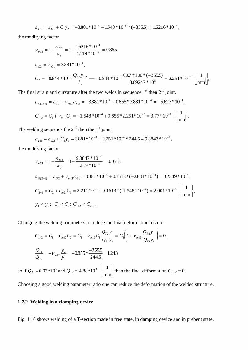
1.7.2 Welding in a clamping device
Fig. 1.16 shows welding of a T-section made in free state, in damping device and in prebent state.

Data: QT = ⎡⎣⎢
⎤⎦⎥
950 Jmm
; L = 7 m, E = 2.1*105 MPa, fy = 240 [MPa].
Determination of the gravity center
; yT = 26 mm, y0 = 24 [mm]. ydAA
=∫ 0( )
Determination of the moment of inertia
; Ix = 1.1381*108 [mm4]. I y dxA
= ∫ 2
( )
A
Fig. 1.16 Welding of a T-section made in free state, in damping device and in prebent state
Welding in free state
CQ y
IT T
x
= − = ⎡⎣⎢
⎤⎦⎥
− −0 844 10 1827 103 6. * . * 1mm
,
w CL= =
2
81119. [mm] .
Welding in clamping device
w wII x
'= ξ .
Cross section area and width of the yield zone
A Q b tyT
y= = =143
5 664.
] [mm2 ,

by = 13.3. [mm].
Determination of the gravity center
. ydAA( )∫ = 0
The moment of inertia decreasing the section with the yield zone
, I y dAA
ξ = =∫ 2 81033 10( )
. * [mm4 ]
C CII x
' . *= = ⎡⎣⎢
⎤⎦⎥
−ξ 1658 10 6 1mm
,
w C L' '=2
8,
w wII x
' .= =ξ 1015 [mm] .
It can be seen that w’ < w always, but w ≠ 0 .
1.7.3 Welding in prebent state in a clamping device
Conseder the same T-section in Fig. 1.16.
w w wII
y wL
f Px T
y
= =+ −
0 8 12
,
ξ ε
With the data yT = 26 mm; w = 11.19 mm; ε y =−1119 10 3. *
wP = 77.605 [mm]
The prebending should be in the elastic zone.
The limit prebending deflection is as follow
w C L Lyy y y= = =
2 2
8 88312ε
max
. [ mm],
where ymax = 84 [mm].
Since the prebending deflection is less than the yield deflection, so the result is suitable.
1.8 Weld improvement methods
There are many commonly used improvement techniques to increase the fatigue strength of welded steel
joints (Haagensen 1985, 1996). There is no strong correlation between fatigue strength and yield or

tensile strength for welded joints because the fatigue life is dominated by crack propagation and the
fatigue crack growth rate is practically independent of the steel strength (Barsom 1971, Maddox 1991).
The crack growth rate is slower in improved welds. The decrease of crack growth rate can be achieved
either by the removal of large defects, by a reduced stress concentration at the weld toe, or the crack
growth is retarded by compressive residual stresses.
Fig. 1.17 Reasons of fatigue cracks
Fig. 1.18 Stress concentration
The reasons of fatigue cracks are illustrated in Fig. 1.17. The stress concentration or notch effect is one
reason why cracks initiate at the weld toe. The detailed stress analysis shows that the stress concentration
factor of the welded joint in Fig.1.18 is lower than that for the plate with a hole. Other weld defects, such
as cold laps as shown in Fig.1.17, reduce the fatigue strength. A third contribution to the reduction of the
length of the crack initiation stage are the high tensile residual stresses. The waviness of the weld toe in
the length direction has considerable influence on the fatigue life (Chapetti & Otegui 1995).
Methods to extend crack initiation life, are as follows:
a) reducing the stress concentration factor of the weld by improving its shape,
b) removing the crack-like defects at the weld toe, and
c) removing the harmful tensile welding residual stresses or introducing beneficial compressive stresses
in the toe region.
Modification of the weld shape also reduce the severity of the weld toe defects, weld improvement
methods can be placed in two broad groups:
- Weld geometry modification methods
- Residual stress methods
We describe only some methods, which are mainly used in industrial applications.
1.8.1 Weld geometry modification methods
Weld profile control, i.e. performing the welding in such a manner that the overall weld shape gives a
low stress concentration and the weld metal blends smoothly with the plate.
Improved welding techniques, such as weld profiling and the use of special electrodes can reduce the
weld toe defects.
Improved weld profiles means that a low stress concentration factor is aimed for by controlling the
overall shape of the weld to obtain a concave profile and by requiring a gradual transition at the weld toe.
Weld toe grinding
Grinding can be carried out with a rotary burr grinder or disc grinder, the former requiring much
more time and therefore incurring higher costs. The lower stress concentration factor and the removal of
crack-like defects at the weld toe generally give large increases in fatigue life for transverse welds,
around 50-100 percent at long lives (N > 1 million cycles).
Tungsten inert gas (TIG) or plasma arc remelting.
Remelting of the weld toe using either TIG or plasma welding equipment generally results in large
gains in fatigue strength. The smoother weld toe transition reduces the stress concentration factor; the
slag inclusions and undercuts are almost completely removed, and the increased surface hardness in the
remelted zone contribute to the higher fatigue strength [Kado et all (1988), Ohta (1988)]. In addition the
original residual stress field is altered.
Standard TIG dressing equipment is used, usually without any filler material. TIG remelting also
introduces a residual stress field, which like the welding process used for depositing the weld metal,
usually gives tensile stresses at the surface (Lieurade et al 1992, Lopez Martinez & Blom 1995). The
magnitude of the improvement depends primarily on the joint severity and base material strength. The
improvements for medium strength steels are about 50 - 70 % over the as-welded strength.
Plasma dressing generally gives better results than TIG dressing, due to the higher heat input and the
larger pool of melted metal.

1.8.2 Residual stress methods
Improvement in fatigue behaviour can be obtained by removing welding residual stresses by postweld
heat treatment, especially if the applied load cycle is wholly or partly in compression. The largest benefits
are obtained if compressive residual stresses are introduced.
Hammer peening
Hammer peening is usually performed with a pneumatic hammer fitted solid tool with a rounded tip
of 6-14 mm radius. A similar technique consists of using a wire bundle instead of a solid tool. The solid
tool gives a far more severe deformation and gives better improvements than either wire bundle or shot
peening (Gurney 1979). Optimum results for hammer peening are obtained after four passes.
Ultrasonic peening
This is a new method, and as for other improvement methods, the magnitude of improvement varies
with material, type of joint and type of loading, but the improvement is about 50 - 200 % (Trufiakov
1995).
Shot peening
In the shot peening process the surface is blasted with small steel or cast iron shots in a high velocity
air stream, producing residual surface stresses of about 70 to 80 % of the yield stress. Results from
fatigue tests on shot peened welded joints show substantial improvements for all types of joints, the
magnitude of the improvements varying with type of joint and static strength of the steel. The
improvement is about 30-100 % increase in fatigue lives in the long life region (Grimme et al 1984,
Haagensen 1992).
Even larger improvements may be obtained when techniques from the two main groups are combined.
The effectiveness of most improvement methods is highest in the long life, low stress part of the S-N
curve. In the short life region, where the local stress at the weld toe exceeds the yield limit the effect of
most improvement methods is small or non-existing, this is particularly true for the residual stress
methods. Since most structures are designed to the long life part of the S-N curve these improvement
techniques can have a great advantages. Fatigue strength improvement is best measured by the fatigue
strength at 2 million cycles.
Comparison of costs (Godfrey & Hicks 1987)

If we choose hammer peening as unity, then shot peening is approximately 1.5, disc grinding is 5 and
TIG dressing is 3 times more expensive. If we compare the efficiency of the techniques we find that
hammer peening and grinding combined with hammer peening gives the largest improvements, in excess
of 100 % increase. A 60 % increase over the as-welded design curve is therefore proposed.