Residual Value Risk and Insurance:

Evidence from the consumer automobile industry

Gerson M. Goldberg College of Business

New Mexico State University Las Cruces, NM 88003-8001

gmgold@nmsu.edu Phone: (575) 646-2954

Shantaram P. Hegde*

School of Business University of Connecticut

Storrs, CT 06269-1041 shegde@business.uconn.edu

Phone: (860) 486-6870 Fax: (860)-486-0889

March 27, 2009

*Contact author. Preliminary, do not quote or cite without the permission of the authors.

Residual Value Risk and Insurance:

Evidence from the consumer automobile industry

Abstract

Recent press reports note that consumer automobile lessors have suffered huge losses mainly due to the use of inflated residual values coupled with sharp drops in used vehicle prices. Assuming frictionless markets, we employ the Black-Scholes European put option pricing model to develop estimates of residual value insurance premium for used automobiles. Based on a sample of wholesale prices of used cars for three popular models over 1990 to 2006, we find that the average insurance premium ranges from 1.6% to 2.5% of insured value for two to five year policies. Further scrutiny suggests that our premium estimates are robust to analyst forecasts of residual values, used car index prices, and default risk. Finally, our evidence indicates that average ex-post residual value losses range from 7% to 12% due to aggressive subvention during our sample period. While buying insurance would have been highly effective in protecting retail automobile lessors against such losses, it would have imposed huge underwriting losses on residual value insurers.

3

Recent news reports from the automotive industry indicate that the Detroit Three

automakers and their financing units have incurred huge losses in their leasing business, mainly

due to falling resale values on trucks and sports-utility vehicles leased a few years ago. For

instance, on August 11, 2008, Automotive News reported that General Motors Acceptance

Corporation incurred $716 million in write-downs related to its North American lease business

and its parent General Motors Corporation took a $2 billion second-quarter charge because of

residual value losses, see www.autonews.com. The objective of this study is to investigate the

residual value exposure of vehicle leasing firms and how to insure against this risk.1

Leasing is an important financial innovation for acquiring durable goods and it accounts

for nearly a third of the new industrial and commercial equipment and consumer vehicles sold

annually in the United States.2 Broadly, a lease contract transforms a risky new real asset into

two components, a front-end financial asset with fixed periodic payments over a known term of

T years and a back-end residual real asset that covers its economic life beyond lease termination.

In general, the residual value refers to the expected value of the T-year used asset at the end of

the lease. The front-end lease typically has an annuity-like structure with monthly fixed

payments and it exposes the owner of the new asset, called the lessor, primarily to interest rate

risk and credit risk of the counterparty. The main source of uncertainty embedded in the back-

end residual asset is the risk that the future market value of the underlying asset at lease

termination will vary from the projected residual value stated in the lease contract at lease

origination. This price fluctuation is commonly known as residual value risk. Thus, a lease is a

loan in �kind� � loan of a real asset (a durable good) that depreciates over time. As a �real� loan,

it exposes the lessor (lender) to not only default risk on the contractual lease payments but also to

fluctuations in the lease-end residual value of the underlying asset. It parcels out (i.e., unbundles)

the risk of economic ownership of a new real asset into a hybrid structure consisting of front-end

fixed-rate periodic lease cashflows and an uncertain final (balloon) payment. In so doing, it

allows the lessor to restructure the time profile of ownership risk into two tranches � a near-term

debt-like security typically with lower risk (analogous to a senior tranche in a collateralized debt

4

obligation (CDO)) and a deferred equity representing residual economic ownership (similar to

the junior or equity tranche in a CDO).3

As compared with credit risk and interest rate risk, residual value risk is the greatest

uncertainly in lease financing because forecasting residual value T years in advance is fraught

with errors. Further, the magnitude of the residual value at risk decreases with the term of the

lease as a fraction of the economic life of the underlying asset (whereas default and interest rate

risks tend to increase with the lease term). While the owner of the asset, called the lessor,

typically bears the default and interest rate risks associated with the contractual lease payments,

the allocation of residual value risk depends upon the type of lease contract.

In an open-end lease, the user of the asset, called the lessee, is obligated to compensate

the lessor if the market value of the underlying asset at lease expiration drops below the

projected residual value. In other words, the lessee is required to guarantee the underlying asset

at lease maturity at the fixed residual value even though its market value may be lower.4 The

lessee issues a residual value guarantee, which is essentially a real put option, to the lessor in

exchange for a real call option to purchase the underlying equipment at the residual value at

lease termination.5 These embedded real options expand the lessor�s core portfolio to include (a)

the present value of lease payments (the front-end asset) and (b) the deferred residual asset

bracketed by the put and call options. The bundle of assets in (b) can be characterized as one

resembling a long position in a stock with a value equal to the present value of the residual value

of the underlying real asset, a long position in a put option on the underlying equipment with a

strike price equal to the residual value and term identical to the lease period, and a short position

in a call with an identical strike price and term to expiration to that of the put option. If we make

the reasonable assumption that the residual value is set equal to the forward price of the

equipment for delivery at lease termination, it is straight forward to show from the standard

European put-call parity relation in the financial options literature that the package comprising

the long residual asset, long put and short call is comparable to a riskless bond. Thus, the

lessor�s overall portfolio covering both (a) and (b) positions consists of the sum of present values

5

of a riskless T-year maturity zero-coupon bond and a coupon-like bond representing the lease

cashflows.6 The net effect of these arrangements is that the lessor is returned to a position very

similar to the one associated with outright sale of the underlying asset on credit.

In sharp contrast, a closed-end lease contract exposes the lessor to residual value

uncertainty. The classic example of a closed-end lease is a consumer automobile lease contract

with two to five year terms. Residual value guidebooks show that passenger vehicles are worth,

depending upon their make and style, from about 20% to 60% of their initial purchase price after

five years (see www.Edmunds.com and www.kbb.com). Therefore, unlike the typical equipment

lease contract, the consumer lease for new automobiles exposes the closed-end lessor to sizeable

residual value risk � the risk that the market price of the leased vehicle at the end of the lease

period varies from its predetermined residual value.7 Even if we ignore credit risk associated

with the fixed monthly lease receipts over T years, the closed-end lessor holds an ill-diversified

risky position in the underlying residual asset.8 In contrast, the residual value guarantee issued by

the open-end lessee in the equipment segment is typically a small part of his overall portfolio and

hence relatively more diversifiable.

Similar to an open-end equipment lease, a closed-end retail auto lease typically grants a

purchase option allowing the lessee the right to buy the leased car at the fixed residual value at

lease termination. Consequently, the core portfolio of a vehicle lessor contains a long position in

the present value of lease payments, another long position in the present value of the T-year

residual value of the underlying vehicle and a short position in the call option. Setting aside the

stream of lease payments, the remaining two elements of the portfolio are analogous the standard

covered call writing strategy in the literature on financial options. As a writer of a call option on

the used car, the closed�end lessor sacrifices not only the upside potential of market value

exceeding the residual value of the used vehicle but also faces the downside risk � the risk that

the terminal market value drops below the residual value. Again, from the standard European

put-call parity relation in financial options, the lessor�s core portfolio (excluding the relatively

simpler present value of lease payments) can be characterized as one resembling a long position

6

in a riskless bond with a value equal to the present value of the residual value and a short

position in a put option with a strike price equal to residual value and term identical to the lease

period. In other words, his long residual asset - short call position is similar to holding (risky)

debt subject to default risk if the residual value varies from the forward price of the underlying

asset. It is worth emphasizing that this default risk inherent in the portfolio in (b) is separate

from the credit risk attributable to the lessee in package (a). The written put option reflects that

the lessor is effectively self-insuring against the residual value loss. Evidently, a short put

position can entail huge losses when the put exercise price is high (relative to the forward price

of the used asset), the lease term is long, and the underlying used car price suffers a sustained

sharp decline. Notice that the lessor�s counterpart who sells the durable good outright on credit

does not face the risk associated with a short put position.

News reports indicate that in the early-1990s consumer auto lessors in general and

captives (i.e., financing arms of automakers, such as General Motors Acceptance Corporation

(GMAC), Ford Motor Credit Corporation (Ford Credit), DaimlerChrysler Financial Services

(Chrysler Financial), Toyota Motor Credit Corporation (Toyota Financial Services), etc.) in

particular, used unduly high residual values to lower monthly lease payments and thereby boost

the lease volume.9 This practice of using aggressive residuals, known as subvention or

subsidized residuals, led to a leasing boom, but it haunted the leasing industry in the form of

increased vehicle returns as the vehicles came off lease in subsequent years with huge

remarketing losses attributable to inflated residual values.10 Table 1 reports survey data from the

Association of Consumer Vehicle Lessors (ACVL), a national trade association of the largest

manufacturer and import distributor captive finance companies, banks, and independent leasing

companies accounting for approximately 85% of all consumer vehicle leases in the U.S.

[Table 1 here]

In 1997, the survey participants leased 3.20 million vehicles with a total dollar volume of

$74 billion at an average capitalized cost per vehicle of about $25,000. The new lease volume

7

reported by these lessors fell to 1.89 million vehicles by 2002. On average, 44% of vehicles

reaching lease end were returned to lessors in 1997, which increased to 57% by 2002. Of these

returned vehicles, 77% and 92% ended up with residual value loss in 1997 and 2002,

respectively.

The unweighted average residual loss per returned vehicle (including the gain on

vehicles) across all ACVL survey participants rose from $1,305 to $2,982 (estimated) during that

period. The end-of-term (EOT) residual loss per returned vehicle weighted by the number of

vehicles returned to each lessor stood at $1,835 in 1997 and $3,269 in 2002, implying that

(captive) lessors with larger lease volume suffered sharper residual loss than those with smaller

volume (banks and independent lessors). The increasing time trends in the return rates and

residual loss are consistent with the expectation that larger losses lead to more EOT returns in

closed-end leases. From the last two rows, the lease term varies from an unweighted average of

38.6 months and a weighted average of 32.3 months in 1997 to 46.5 (unweighted) and 41.4

(weighted) months in 2002. The average observed increase of about nine months in lease terms

over time is consistent with the observation that many lessors place less emphasis on short-term

leases because the percentage of vehicles returned at lease end with residual loss is generally

higher on the shorter terms than the longer terms. The shorter weighted lease terms suggest that

the (larger) captive lessors tend to write more of two- to four-year leases whereas the (smaller)

bank and independent lessors concentrate on four- to six-year leases, see Astorina and Mrazek

(2000), Wolfe, Abruzzo, Olert, and Behm (2001), and Vertex Consultants, Inc. (1998).11

Panel B of Table 1 shows the rate of early terminations by lease term for leases originally

scheduled to terminate in 1996 through 1999. The decline in the rate from 1996 to 1998

indicates that more leases reached end of term in 1998 than in 1996 for almost all lease

maturities, probably because fewer leases were in-the-money (i.e., market value of used vehicle

greater than its contractual residual value) during the lease term. Analysts note that in order to

mitigate the steep loss due to aggressive subvention, car makers and dealers resorted to

extending proactive early lease termination programs under which lessees were given attractive

8

�loyalty� offers to purchase, trade in or refinance leased vehicles in the last year prior to maturity

of the lease. Residual value losses will generally be smaller and less frequent when a longer-

term lease terminates early because the vehicle has had less time to depreciate. Further, closed-

end leases require the lessee to make whole the lessor upon early termination, see Astorina and

Mrazek (2000), and Kravitt and Raymond (1995). This policy seems to explain the increase in

the early termination rates for the four- and six-year leases in 1999.12

A lessor may manage residual value risk directly by buying a residual value insurance

policy, a new insurance product introduced back in the late 1970s. Under this arrangement, the

insurer promises to indemnify the policyholder, in exchange for a fixed initial premium, if the

value of the insured asset falls below the residual value at lease termination.13 The purchase of

residual value insurance adds a long put option on the underlying asset to the close-end

consumer auto lessor�s portfolio and thus offsets the short put position. While this mechanism

for risk transfer coupled with fair pricing of residual value insurance leads to hedging benefits

for lessors,14 news reports indicate that several insurance companies suffered large underwriting

losses, due to both higher frequency and severity, on the residual value insurance policies they

wrote in the late 1990s.15, 16

There is a vast literature dealing with many complicated aspects of real world leasing,

such as, tax incentives, accounting treatments, legal issues, and credit risk. However, despite its

pervasive prevalence across the durable assets landscape ranging from autos, aircrafts, railroad

rolling stock, machine tools, computers, construction equipment, truck tractors, trailers, medical

devices, and printing equipment, there is no systematic study of residual value risk and insurance

practices in the academic literature. Since the value of the underlying real assets is quite variable

over the typical two- to ten-year lease terms, financial economics suggests that the long-term

consumer real put option can have significant value. However, the available theoretical and

empirical evidence is sketchy and confined to applied industry sources and sales promotion

materials. In a rare applied treatment we could find, Kolber (1985) describes residual value

insurance as a put option on the underlying asset and notes that premiums for automobile

9

residual value insurance are quite low because of the relatively short term of leases and liquidity

of the secondary market for vehicles. While each policy/risk is underwritten individually (with

costs varying in proportion to the level of risk assumed), he reports that premiums on auto leases

run from 1% to 2.5% of the insured amount. By contrast, lease policies on equipments, which

tend to have less liquid secondary markets and longer lease terms, carry higher premiums,

generally between 5% to 8% of insured value. In the real estate market, the cost of the residual

value policy would generally run from 3% to 6% of the guaranteed property value. However, we

could not find any systematic study to verify the magnitude of self-reported residual losses

suffered by vehicle lessors and advertized residual insurance premiums. The objective of this

study is to quantify (ex ante) the residual value risk and insurance in the consumer automobile

lease market and estimate the benefits of hedging this risk.

Assuming frictionless durable goods markets, we employ the Black-Scholes European

put option pricing model to develop stand-alone benchmark estimates of the residual value risk

and insurance premiums for used automobiles. Based on a sample of wholesale prices for three

popular car models over 1990 to 2006, we find that the average insurance premium ranges from

1.6% to 2.5% of insured value for two- to five-year policies. Further scrutiny suggests that our

premium estimates are robust to analyst forecasts of residual values, used car index prices, and

default risk. Finally, our evidence indicates that average ex-post residual value losses range from

7% to 12% due to aggressive subvention and unexpected sharp declines in used vehicle prices

during our sample period, and buying third party insurance would have been highly effective in

protecting retail automobile lessors against such huge losses. Our primary contribution to the

literature is that we are the first academic study to present a systematic and comprehensive

theoretical and empirical analysis of the residual value risk and insurance in the retail automobile

industry.

The implications of our study go far beyond the leasing industry and extend to the

ongoing debate on the complexity of advanced structured products used to securitize risk and

spread it across many investors as well as the widespread misunderstanding about risk hidden in

10

new products emerging from financial innovations over the last four decades. For instance,

highlighting the hybrid structure of a simple lease contract (with no purchase option or residual

value guarantee), we characterized it as an equity-linked bond. However, there is a danger that

some lessors and investors in securitized lease portfolios would view the security as a regular

bond, thus failing to account for the risk inherent in its equity-link. Such a failure can lead to

excessive risk-taking, especially when lessors adopt loose leasing standards to ramp up lease

volume and rely heavily on debt to fund the lease portfolio. The current banking and insurance

crises suggest that this miscomprehension seems to encompass not only individual and

institutional investors but even the �pros� � the financial institutions that engineer these exotic

products and credit rating agencies and regulators who failed to adequately scrutinize the

creditworthiness and capital requirements of firms that issue these products.

A more complex and extreme case of an exotic financial product is provided by synthetic

collateralized debt obligations (CDOs) which provide default guarantees (insurance) by selling

contracts known as credit default swaps (CDS) on a pool of corporate debt (equivalent to a short

position on a long-term put option on bonds). Press reports indicate that investors � including

school districts, municipalities, charities, pension funds, community and regional banks and

insurance companies have lost billions of dollars in the wake of the recent credit crisis.17 The

current turmoil in credit and financial markets across the globe demonstrates that loose

leasing/lending standards stemming from misunderstanding the complexity of these structures

and the consequent reckless risk-taking has the potential to transform leases into toxic or

distressed assets in environments characterized by steep rise in borrowing costs and sustained

decline in asset prices, thus endangering the health of lessors, banks and insurers as well as

threatening financial stability at large.

Suppose a lessor holds a leveraged lease portfolio − borrows using the self-insured

closed-end lease portfolio (with a written call option) as collateral. This arrangement typically

imposes three types of financial risks on the lessor, similar to the effects of a credit default swap

(CDS) on an insurer that sells protection against default on bonds and mortgages. First, like the

11

swap seller who has to indemnify the counterparty in the event of default, the lessor in essence

compensates the lessee if the used asset price drops below the contractual residual value at lease

expiration. Second, the lender (analogous to the buyer of the swap) has the right to demand

more collateral prior to lease end from the lessor if the underlying used asset declines in value, or

if the lessor�s own credit-rating is downgraded. Therefore, the lessor faces collateral call risk.

Finally, the lessor is obliged to take write-downs on its own books based on the falling market

values of leased vehicles (write-down risk). In light of these similarities, it is perhaps not

unreasonable to characterize the aggressive subvention policies and the resulting large losses

suffered by lessors as soured bets on residual values.

Our analysis and results have implications for federal housing agencies that acquire or

guarantee mortgage loans originated by real-estate lenders. These insurers seek to protect

themselves/taxpayers against loan default losses through loan-level price adjustments

(surcharges on mortgage rates or fees paid by borrowers). Errors in assessing and managing

mortgage default risk expose these guarantors and taxpayers to huge losses.

As noted above, closed-end retail auto lessors typically self-insure the residual value

specified in the lease, which fixes the annual rate of depreciation charged to the lessees. In turn,

they can cover their exposure by buying residual value guarantees offered by third-party insurers.

In the early-1990s, lessors resorted to inflating the residuals to promote lease volume. In a

similar vein, since the mid-1990s insurance companies have aggressively offered a variety of

investment performance guarantees (subject to complex tax penalties, withdrawal restrictions,

and surrender penalties) to ramp up sales of variable-annuity contracts, which amounted to about

$180 billion in 2007.18 At the beginning of 2009, the vast majority of over 22 million variable

annuity contracts in force covering $1.4 trillion in assets offered some type of investment income

guarantee. Often these contracts promise 5% to 7% annual compounded growth for an annual

fee of about 3.5% of the underlying portfolio. The insurers incur gross loss if the decline in the

underlying investment asset values exceeds the annual fee. To manage this risk exposure, they

typically buy reinsurance (i.e., transfer part of the liability due to the guarantees to other insurers

12

for a fee) and buy financial derivatives that hedge the increase in liability for the guarantees

when stock and bond markets fall. Such hedging programs are expensive and require continuous

updates because often the derivative instruments have maturities of one to five years while the

guarantees carry longer terms and can last 30 years. Moreover, media reports suggest that risk

managers have struggled to keep pace with product innovation involving complex guarantees.

Because of gaps in the risk management programs, shares of some insurers have plummeted

under the recent extreme market conditions and they have taken huge charges against earnings to

set aside additional reserves and raised new capital.

It is quite plausible that in some instances the residual value loss suffered by the lessors

and insurers is not simply due to misunderstanding of the underlying risk but the result of

deliberate reckless risk-taking in pursuit of increased incentive compensation for managers or

private benefits of control. We do not pursue these questions because of data limitations. The

used car price data we gathered allows us to address the issue of residual value risk, but it is not

adequate to evaluate the overall profitability of a lease transaction � the sum of residual value

gain/loss and that on the stream of periodic lease payments.

The paper is organized as follows. In Section I, we develop a simple payoff model to

show that a closed-end auto lessor�s main risk exposure can be characterized by a put option on

the underlying used car price and then review the Black-Scholes European call and put valuation

models. Section II explains how we assemble time series of constant quality used car price

prices for three popular car models over 1990-2006 and presents estimates of average prices and

return volatilities. In Section III, we discuss the base case estimates of the residual value

insurance premiums and scrutinize their robustness to alternative measures of used car prices.

Section IV examines the sensitivity of the put option estimates to the key parameters of the

model and adjusts the put value estimates for the possibility of default by the lessee. We discuss

estimates of the end-of-term residual value loss and the benefits from insuring against those

losses in Section V and investigate the effects of inflating residual values in Section VI. Section

VII concludes the paper.

13

1. Residual Value Risk and Insurance as a Put Option

This section describes the payoffs from a typical retail automobile lease contract and

presents a simple frictionless model to illustrate that the value of residual value risk and

insurance can be approximated by a put option on the underlying used asset.

1.1 A Simple Model of Closed-end Lease Cashflows

Consider a simple closed-end lease agreement with no embedded options. A lessor buys

a (new) risky real asset at S(t) at time t = 0 and converts it to two component assets: a lease

contract and a residual asset. The lease instrument is a financial security comparable to a risky

bond with monthly coupon flows equal to lease payments (LP) over the lease term of T years.

By contrast, the residual asset refers to the expected value at time T of the leased real asset. To

focus our discussion on the underlying asset price fluctuations, assume no default by the lessee

and no interest rate risk. As portrayed in Panel A of Table 2, at t = 0 the lessor�s position

consists of the present value of lease payments (PVLP) and the present value of the expected

time T residual value of the underlying asset (PVRV). At the expiration of the lease (time T), the

aggregate value of leased asset consists of the cumulative value of all lease payments (CVLP)

and the prevailing market value of the leased asset (S(T)).19 Unlike an outright credit seller of

the durable asset, the lessor is exposed to residual value risk � risk that the used asset market

value at T, S(T), will vary from its predetermined residual value (RV).

[Table 2 Here]

In Panel B, the lessor sweetens the closed-end lease by offering a purchase option to the

lessee, thus granting the right to buy the underlying used vehicle by paying the residual value at

T. Since the primary focus of our analysis is not on the default and interest rate risks associated

with the periodic lease payments, we will ignore the lease contract cashflows (shown in the first

row of Panel A) in the following discussion and focus on the residual asset cashflows and the

associated option payoffs. The short call caps the cashflow at a known value of RV when S(T) >

RV. However, when the option expires out-of-the money (i.e., S(T) < RV), the lessor�s position

14

is risky, worth only S(T). Notice that this package is effectively a covered call (i.e., long

underlying asset and short call), with the terminal value equal to the minimum of [S(T), RV].

That is, the lessor loses the upside potential while exposed to the downside risk. This is

analogous to the position of a corporate (risky) zero-coupon bondholder who receives full

payment at maturity if the value of firm�s assets exceeds the face value of the bond, otherwise

the value of assets (see Merton (1974)). As compared with the outright credit seller of the

durable asset who faces default risk attributable to the lessee, the closed-end lessor downside

price fluctuation in the underlying used vehicle.

The concentrated downside risk of the residual asset presents a challenging risk

management problem because the lessor is typically undiversified. The lessor can hedge this

exposure by buying residual value insurance via a put option on the residual asset. From Panel

C, the terminal value of the residual asset, short call, and long put positions is equal to RV. In

other words, the lessor gives up both the upside potential and the downside risk and converts the

risky real residual asset into a riskless bond. Notice that we have implicitly assumed that at t = 0

the lessor sets RV equal to the price of a forward contract that calls for delivery of the residual

asset at T such that the put and call have equal values, C = P. That is, the closed-end lessor is

long the residual asset and short the forward contract. Further, by purchasing the residual value

insurance and selling the purchase option, the lessor has transformed the closed-end auto lease

into an open-ended operating lease common in the equipment market where the lessee

guarantees the residual value in exchange for the purchase option.20

In summary, the above analysis illustrates how the key elements of a typical lease

security vary profoundly from that of an equity-linked bond to a combination of a risky and a

riskless bond depending upon the options embedded into the structure. It highlights the essential

nature of residual value risk faced by the closed-end lessor, the cost of insuring which can be

approximated by the value of the put option on the residual asset. It is worth noting that this risk

is more perilous and quite different from the credit risk that an outright seller of the underlying

asset faces from the lessees because the latter is relatively more diversifiable.

15

1.2 Estimating the Value of Residual Value Insurance in Frictionless Markets

In order to focus on the evaluation of residual value risk and insurance, we make the

standard assumption of frictionless capital markets � the underlying asset market is without

moral hazard, information asymmetry, and other frictions such as default. Further, we ignore the

portfolio choice problem that views the underlying asset and the embedded real options as a

package in conjunction with the firm�s broader portfolio of assets and liabilities, and treat the

lease-end put option as a stand-alone option. Admittedly, these assumptions are unrealistic.

Many studies show that durable goods markets are characterized by moral hazard and

asymmetric information problems, and the embedded options can play an important role in

mitigating these frictions and thereby improve consumer welfare, see Akerlof (1970) and Hendel

and Lizzeri (2002). Further, leasing exacerbates agency costs by separating ownership and

control of the underlying asset. As Smith and Wakeman (1985) and Waldman (1997) note, the

purchase option serves to weaken the moral hazard problem by giving the user an incentive to

take care of the asset. Since an adequate treatment of the information and agency issues is quite

complex, we ignore them and concentrate on generating frictionless market benchmarks for the

residual value insurance premium.

Default risk is another important market friction in our context because the value of the

underlying used car can fall below the outstanding lease obligations in the event of default.

However, we believe the default option is less valuable as compared with the residual value risk

because the closed-end lessor owns the leased vehicle, and the repossession of a leased asset is

easier than foreclosure on the collateral of a secured loan, see Eisfeldt and Rampini (2008) and

Giaccotto, Goldberg, and Hegde (2007). Therefore, first we will focus on the valuation of the

lease-end put option ignoring default risk. Subsequently, we will scrutinize the robustness of our

base-case put option estimates to default risk.

Although our focus is on the put option on the residual asset as a measure of the residual

value insurance premium, in practice, retail auto leases contain two additional embedded options,

namely, a compound cancellation option and a European purchase option at lease expiration,

16

both granted to the lessee. Assuming no prepayment penalties, Schallheim and McConnell

(1985) model the fair value of the cancellation option as the difference between the present value

of rental payments on a cancelable lease and those on a noncancelable lease of identical maturity,

where the two sets of rental payments are discounted at the risk-free rate. Their numerical

analysis of five- and seven-year leases shows that the cancellation option can have significant

value. However, Giaccotto et al. (2007) observe that in practice the cancellation option is of

negligible value because lessors commonly levy an early-termination penalty that is determined

in such a way that the lessee can never benefit from variations in the market price of the used car.

Accordingly, in the analysis that follows we will assume away the cancellation option.21

McConnell and Schallheim (1983) show that in the context of a noncancelable lease with

an option to buy the used asset at lease expiration, the value of the purchase option, C, is given

by

)()( 21 dNXedNSC rT−−= (1)

where S is the present value (discounted at the risk-adjusted rate) of the expected market price of

the leased automobile T periods from now, X is the exercise price, r is the riskless rate, 2σ is the

variance of the rate at which the automobile depreciates over time, N(.) is the univariate

cumulative standard normal distribution evaluated at TTrXSd σσ /])2/()/[ln( 21 −+= and d2

= d1 � Tσ .22 This is the familiar Black and Scholes (1973) European call option pricing

model on a non-dividend paying stock.23 Notice that the underlying asset price, S, is the present

value of the expected depreciated asset value at T and hence is not directly observable at time t =

0.24 Further, we need to make no explicit adjustment for the economic value of the service flow

(i.e., dividends) derived from the use of the automobile because we use the (present value of) the

residual asset, which is comparable to the dividend-adjusted stock price, as the asset underlying

the call option. Applying the above model to the wholesale used car price data, Giaccotto et al.

(2007) report that the embedded call option has considerable value, on average about 16% of the

market value of the underlying used vehicles.

17

Giaccotto et al. (2007) do not estimate the value of the put option. Following their

framework, we obtain three alternative estimates of the used car wholesale prices to proxy for the

value of the underlying asset and estimate the lease-end put option value, P, by applying the

Black-Scholes (1973) European put valuation model:

)()( 12 dNSdNXeP rT −−−= − (2)

We use these put option estimates as the frictionless market benchmarks for the residual value

insurance premium.

2. Sample Construction

In the context of a conventional put option on a publicly traded common stock, the

underlying stock price is known, the strike price (denoting the level of protection desired) is a

choice variable, and the volatility of stock returns over the typically shorter terms of the option

can be estimated with a reasonable degree of confidence by computing volatility implied by the

market data on well-traded options. In contrast, as emphasized in the previous section, obtaining

reliable estimates of these parameters in applications involving real options on durable goods

with illiquid and fragmented secondary markets poses a formidable challenge. Specifically, in

our case the market price of the underlying vehicle at the lease end in T years is unknown at the

current time t = 0 when a lease contract is initiated. Further, the absence of a liquid forward

market in used vehicles renders it difficult to choose the �right� strike price. Finally, without the

availability of time series of traded used car prices and options, estimating the volatility of

returns on the underlying real asset is fraught with errors. Therefore, assembling reasonable

estimates of the inputs S, X, and σ is a complex empirical task in this paper.

2.1 Description of ALG and NADA data

To generate representative estimates of the residual value risk and insurance, we select

three of the best-selling nameplates in the passenger car market in the United States during the

1990s: General Motors Saturn, Honda Civic, and Toyota Camry.25 These car models were the

most popular body styles and relatively comparable from one year to the next. These

18

characteristics allow us to minimize the effects of quality and style changes typically introduced

by manufacturers at the beginning of each model year, as well as to study both domestic and

foreign brands.26

As shown in Table 1, approximately 50% of leased cars are returned at lease termination

on average and are then disposed off in the wholesale used car market. We obtain the wholesale

prices of used cars from two primary sources of data, Automotive Lease Guide (ALG)27 and the

N.A.D.A. Official Used Car Guide (NADA).28 Base-level monthly wholesale used car prices

(which represent averages of wholesale used car prices reported by dealers) are taken from the

Eastern Edition of NADA for the period November 1990 through November 2006. Further, we

gather annual used car residual values from the November/December Northern Edition of the

ALG for 1995 through 2006. ALG proclaims that its residual values are based on an objective

depreciation rate for the given model (as evidenced by its historical performance), and subjective

expert opinion of how the new model will fare relative to its competitors. However, the ALG

residuals do not account for unusual wear and tear and the direct expense of termination, both of

which are lease-specific. These residual values are widely regarded by the leasing industry as

the best estimate of the expected wholesale value at the end of T years.

2.2 Constant Quality and Maturity Adjustments

From Table 1, retail auto leases typically carry terms varying from two to five years.

Accordingly, we consider a sample of T-year leases on brand new cars signed each November

from 1995 through 2006, T = 2 to 5 years. To price the embedded put option, we need to

estimate the volatility of T-year used car price changes. Since manufacturers introduce new car

models yearly, typically by the month of November of the prior year, we need to adjust the base-

level NADA used car prices and ALG residuals for optional equipment and mileage to maintain

roughly constant quality over our study period. Specifically, price adjustments are made to

ensure that the physical characteristics of automobiles (e.g., automatic transmission, air

conditioning, etc.) remain constant over the study period. Moreover, we follow ALG and adjust

19

reported prices to ensure that the two-, three-, four-, and five-year-old cars have odometer

mileages of 30,000, 45,000, 60,000, and 75,000, respectively.

Next, similar to the formation of a constant maturity bond, we construct an approximately

constant quality monthly time series of used car prices holding age fixed at T years. For

example, consider T = 2 and t = November 1991, when the 1990 model cars (introduced by

November 1989) are two years old. We gather monthly quality-adjusted prices for this two-year-

old car for the next 12 months. Advancing to November 1992, the 1990 model year vehicle

turns three years old and no longer qualifies for the two-year price series. To maintain the term

of the price series at approximately two years, we switch to monthly prices for a 1991 model car

in November 1992. This switching process is repeated for each T-year-old car every November

until the end of the sample period in 2006 to generate the average constant quality and maturity

price time series for three-, four-, and five-year-old cars.

2.3 Estimates of NADA Used Car Prices and Price Volatility

We present in Table 3 summary statistics on NADA monthly wholesale constant quality

prices for two- to five-year-old cars for the three models from November 1990 to November

2006.29 From the second row of the last (Total) column, we have 1908 monthly price

observations across the three car models. The mean (median) price of constant quality used cars

in our sample ranges from $6,090 ($6,125) for a five-year-old car to $9,963 ($9,700) for a two-

year-old car. There is considerable price variability across car models, maturities, and time as

reflected by the standard deviation estimates varying from $1,197 for T = 5 to $1,594 T = 2. The

rest of the table presents price distribution statistics for each of the three car models.30

[Table 3 here]

As Pashigian, Bowen, and Gould (1995) and Pashigian (2001) observe, retail prices for

new cars are higher in November of each model year when automobile companies launch their

new models and then decline during the season. Consistent with the decline in new car prices,

the residual factor applied to MSRP tends to decline over the model year, see Angel (1997). We

20

observe a similar seasonal pattern in our sample of wholesale used car prices. The distribution of

prices reveals a monthly seasonal plus a sharp spike caused by the introduction of a new model.

Further, while the amount of within-year economic depreciation seems to be fairly stable

throughout the sample period, the November spike appears to be much smaller in the latter part

of the sample period. Following Giaccotto et al. (2007), we incorporate both sources of variation

by using annual differencing of the monthly time series and calculating the continuously

compounded annual percentage price changes from overlapping observations. To estimate the

standard deviation, σ, in November 1995, we use the NADA monthly constant quality used car

prices from November 1990 to November 1995. Subsequently, rolling estimates of σ are

generated in each November by utilizing all prior price data.

The estimates of the annual standard deviations of percentage changes in NADA prices

provide a key component of residual value risk and are reported in Panel B. From the first row,

our estimates of annual standard deviations across all models increase from an average of 8.42%

for a two-year-old car to 10.93% for a five-year-old car. The overall sample average is 9.73%.

Of the three car models, Saturn has the largest annual standard deviation of 13.34%, while Civic

has the lowest estimate of 6.34%. For all the three makes, the older the used car, the greater the

standard deviation.31 In comparison, Ibbotson Associates (2000) report the following annual

standard deviation estimates of realized returns for different stocks and bonds: small company

stocks, 33.6%; large company stocks, 20.1%; long-term corporate bonds, 8.7%; long-term

government bonds, 9.3%; one-year U.S. Treasury bills, 3.2%; and annual inflation rates, 4.5%.

Quigg (1993) finds that implied annual standard deviations for individual commercial property

range from 18% to 28%. Thus, used car prices in our sample are far less volatile than common

stock prices or real estate prices; their volatility seems closer to that of intermediate-term

government and corporate bonds.

The final input we need for the estimation of the residual value insurance premium is the

riskless rate. We collect yields to maturity on Treasury notes from Bloomberg Professional.

21

Over 1995 to 2006, these rates averaged 4.23%, 4.41%, 4.56%, and 4.70% for two-, three-, four-,

and five-year terms, respectively.

3. Estimates of Residual Value Insurance Premium

3.1 Premiums Based on Wholesale Used Car Prices

The above estimates of the constant quality NADA prices, their annual standard

deviations, ALG residuals and interest rates are used as proxies for S, σ, X, and r, respectively, in

the European put option model (equation (2)) for T = 2 to 5 years. We compute the values of T-

year puts for each of Camry, Civic, and Saturn in November of each year t, from 1995 through

2006. This yields 139 put option estimates.

[Table 4 here]

From the last column of Panel A in Table 4, the grand mean (median) of put premium is

$149 ($83), which amounts to 2.1% (1.0%) of the underlying asset price. There is considerable

variability in put value estimates across car models and lease terms, as reflected by the overall

standard deviation estimate of 3.2%. In proportion to the insured value (the strike price as

proxied by the ALG residual value), the grand mean and median put option estimates are 1.9%

and 1.0%, respectively. Further, our overall estimates show that the median value of put options

increases from 0.9% of the insured value for a two-year term to 1.3% of insured value for a five-

year policy. Bear in mind that in addition to term of the insurance policy, the current value of

the insured asset (i.e., the used car price) and the amount at which it is insured (i.e., the strike

price) change across k = 2 to 5 years in our sample. The mean intrinsic value of the put option,

PIV (defined as the maximum of [(X � S), 0]), is $445, which is much larger than the mean time

value (measured as PTV = P � PIV) of �$295. This decomposition shows that in our sample the

strike price (proxied by the ALG residual value) often exceeds the NADA used car price by a

considerable margin. This implies that the used car is on average insured at a higher value than

its prevailing market value, which increases the insurance premium. We scrutinize the extent of

22

upward bias in the residual value insurance premium estimates by generating at-the-money (i.e.,

S = X) put values in the next section.

In the rest of Panel A, we present estimates of the European call options derived from

equation (1). Across all car models and maturities, the mean call value is $1,134 or 13.2% of the

underlying used car price. Thus, the embedded calls on used vehicles are on average worth far

more than the put options with identical terms. Moreover, the decomposition indicates that the

average intrinsic value of the call, CIV, is $216, in comparison to the mean time value of $918.

These estimates are comparable to those reported by Giaccotto et al. (2007).

The estimates of put values for the three car makes in Panels B through D show

considerable variability. The median put option estimates as percent of the insured value of

underlying used cars are 1.1%, 0.5%, and 1.9%, respectively, for Camry, Civic, and Saturn.

Within each car type, the average insurance premium estimates tend to increase with the term of

the policy. These estimates are comparable to the residual value insurance premiums on auto

leases of 1.0% to 2.5% of the insured amount quoted in industry circles, see Kolber (1985). For

2004, R.V.I. Guaranty Co., Ltd. and its subsidiary R.V.I. America Insurance Co., which are

recognized as the leading global providers of residual value coverage, report gross premium in

force of $89 million on an insured portfolio of $8.7 billion in passenger vehicles, which amounts

an average premium of 1%, see www.fitchratings.com and www.moodys.com.

3.2 Premiums Based on ALG Residuals

The above analysis uses the NADA wholesale market prices and ALG residuals to proxy

for S and X, respectively. An alternative source of used car price forecasts is ALG, which is

viewed as the auto industry leader in setting residual values and has released annual awards for

cars, trucks, SUVs, and minivans that rank high in preserving their values over time. Many

financial institutions use ALG�s figures to price their lease contracts. Therefore, we regard the

ALG residual values as expert analyst forecasts of the T-year ahead used vehicle market values.

To scrutinize the robustness of the put option estimates in hand, we use the ALG constant quality

residual values to proxy for both S and X in this subsection. This experiment yields estimates of

23

at-the-money put prices.32 We have twelve annual observations for each T = 2, 3, 4, and 5 years

for each of the three car makes, resulting in 144 observations. The overall mean (median) ALG

constant quality used car price in our sample is $8,883 ($8,775), see Panel A of Table 5. Given

the small number of observations, we use ex post standard deviations of percentage changes in

the ALG used car prices. From Panel B, the grand mean annual standard deviation is 8.36%,

ranging from a low of 6.16% for Camry to a high of 11.93% for Saturn.

[Table 5 here]

The grand mean (median) value of at-the-money puts is $114 ($100). Expressed as a

percent of the insured value X, the overall mean and median estimates are 1.5% and 1.2%,

respectively. Further, these averages tend to increase across the term of the policy, T = 2 to 5

years.

3.3 Premiums Based on a Used Car Price Index

Until now, we have focused on put option estimates of the three individual vehicles.

Since lessors commonly hold broadly diversified lease portfolios consisting of vehicles of many

makes, models, and styles and insurers focus on large portfolios with adequate spread of risk, it

is of interest to estimate the value of an index put option on used car prices. To this end, we use

the used cars and trucks component of the Consumer Price Index (CPI), published monthly by

the Bureau of Labor Statistics, U.S. Department of Labor. The index is comprised of a sample of

480 used vehicles from two through seven years of age. It uses monthly sale prices obtained

from N.A.D.A. Official Used Car Guide, which are adjusted for depreciation of the vehicles.

Based on a three-month moving average of the current and prior two-month depreciation-

adjusted prices, the used car price index is calculated as a monthly price relative using 1982-

1984 as base years.

To conduct this index put experiment, ideally we would like to extract the continuously

compounded percentage price change in used car prices to approximate the historical standard

deviation for use in the index put option estimation. However, it is difficult to extract the

24

underlying monthly used car price series from the published index values. As a rough

approximation, we back out the quarterly changes in the monthly used car price relatives from

the entire published series of index values and compute rolling annualized standard deviations

for each November during our sample period. These estimates vary from 10.5% to 12.3%.

While we realize that these figures provide potentially biased estimates of the volatility of the

used car market portfolio, they seem comparable to the overall standard deviation estimate of

9.74% for our limited sample of three car makes reported in Panel B of Table 3. The fact that

they are slightly higher in magnitude is perhaps attributable to the weaker quality and higher age

limits (up to seven vs. five years) of the vehicles covered by the used car index sample.

Next, we compute the NADA sample mean prices of T-year used cars across the three

automakers and the corresponding ALG residual values in November 1995. Armed with these

representative sample mean values of S, X, T, and r, we use the common index portfolio standard

deviation estimate to generate put option values based on the used car price index. Moving on to

November 1996, we age the T-year sample mean car values from 1995 using the used car price

index and gather our sample-specific average ALG residuals. These revised estimates of S and X

are used along with the rolling index standard deviation estimate and updated r to produce the

next set of index put values. Repeating this process through November 2006, we obtain the

index put results presented in Table 6.

[Table 6 here]

From Panel A, the grand mean estimate of the index used car price and the strike price

are $7,223 and $7,488, respectively, as compared with our sample wholesale mean price of

$8,179 (Panel A of Table 3) and strike price of $8,883 (Panel A of Table 5). The overall mean

of the index portfolio puts is $280, which amounts to an average premium of 3.7% of the insured

value on a 3.5-year term residual insurance policy. These estimates are roughly twice as large as

the sample mean put value of $149 and 1.9% reported in Panel A of Table 4.

25

Given our concern about the upward bias in the index standard deviation of 10.5% to

12.3% used above, we generate an alternative set of standard deviations based on the three-

month moving average of used car index values. As expected, these estimate much smaller,

ranging from 4.68% to 4.95% per annum. In untabulated results, we find that the corresponding

index mean put estimates range from 0.5% to 1.1% of insured value, with an overall mean of

0.8%.

4. Robustness Checks

4.1 Sensitivity Analysis of Put Option Estimates

Since the estimates of the three key parameters (current value of the used vehicle (S),

strike price (X), and volatility of used car price changes (σ)) contain unknown degrees of

approximation, it is important to scrutinize the sensitivity of the reported residual value insurance

estimates to potential errors in the parameter estimates. Moreover, such an analysis helps us gain

better insight into the strategic role of X, T, and r in the presence of moral hazard and

information asymmetry as highlighted by some theoretical models of leasing (see, for example,

Hendel and Lizzeri (1999, 2002)). Table 7 presents the comparative statics results for the put

option estimates reported earlier in Table 4.

[Table 7 here]

We begin with Delta (= ∂P/∂S = N(�d1)), which measures the change in the put option

price for a $1 change in the used car price. Across all car types, the mean (median) delta is �0.20

(�0.17), implying that overestimating the current price of a used car by a dollar would, on

average, depress the value of the put option by $0.20. Similarly, if a lessor sets the strike price

higher by a dollar (i.e., resorts to subvention by inflating the residual value to lower monthly

lease payments and boost lease volume), the grand mean (median) of ∂P/∂X (= )( 2dNe Tr −− )

indicates that the value of the put would be biased upward by $0.16 ($0.16). In other words, the

closed-end lessor increases his exposure to residual value risk by $0.16 on average when he

26

raises the insured value by a dollar to lower monthly lease payments. It is important to stress

that this is a static analysis and as such, it ignores the potential increase in the return rate of off-

lease vehicles that tend to depress the expected value of the used car and thus feeds back into a

higher put option value. Such feedback or positive covariance effects tend to aggravate the

residual value risk.

The next important sensitivity measure is Vega (= ∂P/∂σ = S N′(d1) T , where N′(d1)

denotes the standard normal probability density function), which evaluates the change in option

price for a one unit (= 100 percentage points) change in the volatility of used car price changes.

The grand mean (median) of Vega is 3,218 (3,221). In Panel B of Table 3, our annual price

volatility estimates vary from roughly 8% to 13% with an overall mean of 10%. If the grand

mean underestimates the level of true price volatility by 1%, the observed mean Vega suggests

that the average value of the put option is downward biased by $32.18, holding other things

constant.

Another popular method of subvention in the retail automobile lease market is the use of

cut-rate or below-market financing rates to boost market share. The effect of a one-unit change

in the riskless rate of interest r on P is measured by Rho (= ∂P/∂r )( 2dNeXT Tr −−= − ). Our

sample has a grand mean estimate of Rho equal to �5,605, indicating that if a closed-end lessor

offers a 1% cut-rate lease, he would increase his residual value risk exposure by $56.05 on

average. Finally, the lessor may increase the term of the lease by a year to lower the level of

monthly lease payments. The sensitivity of the put option price to its term to expiration is

measured by Theta (= ∂P/∂T). Its grand mean of 37 indicates that by increasing the lease term

by a full year the lessor increases the residual value risk roughly by $37 (from a mean of $149,

see Panel A of Table 4).

4.2 Adjustment of Put Values for Default Risk

Our analysis thus far has generated stand-alone estimates of the residual value risk and

insurance via the put option valuation model in equation (2) and has implicitly assumed that the

associated lease contract is default-free. However, the closed-end auto lessor�s residual value

27

risk exposure is coupled with the lease contract that is subject to default. If a retail automobile

lessee defaults on the outstanding lease payments, he stands to lose not only the right to use the

underlying used vehicle but also the embedded purchase option (i.e., its value drops to zero).

Moreover, the lessor�s residual value exposure comes to an abrupt end with the lease default, and

he repossesses the underlying collateral to recover the loss on default. In the presence of

counterparty default risk, the adjustment of derivative prices for the possibility of default by

Jarrow and Turnbull (1995) and Hull and White (1995) suggests that the standard Black-Scholes

option pricing model overestimates the value of a lease-end put option that is conditional on the

lessee�s performance on the lease contract. Assuming independence among the lease default

process, the underlying used car price process, and default-free spot interest rate process, these

models show that the value of a put option exposed to credit risk, P*, is equal to the discounted

value of the default-free Black-Scholes put P, where the discount rate is given by the credit

spread, (r* � r) appropriate for the default risk class of the lease. That is,

( )TrrePP −−= ** , (3)

where r* is the risky zero-coupon interest rate reflecting the lessee�s credit risk.33

[Table 8 here]

We collect credit spreads on industrial bonds rated BBB, which vary from 0.47% to

1.94% for two- to five-year maturities. Then we discount the default-free put value estimates

reported in Table 4 by these credit spreads. Table 8 reports the resulting credit risk-adjusted put

values. For the full sample, the median put estimate is $82 (or 0.9% of insured value), as

compared with $83 (or 1%) for put options without credit risk (see Table 4). However, since the

lessee is more likely to default when the underlying used car price is below the contractual

residual value (i.e., the put option is in-the-money), the assumption of independence between the

two processes is violated. The resulting positive correlation induces a downward bias into the

default risk-adjusted put value estimates reported above.

28

In the retail auto lease industry, ACVL (2002) reports that net credit losses (after

recoveries) averaged 48 to 87 basis points (bps) over 1999 and 2002. At the securitized portfolio

level, Volkswagen Auto Lease Trust 2004 prospectus discloses net credit losses (excess of

charge-offs over recoveries) due to repossessions of 0.32%, 0.31%, 0.40%, 0.38%, and 0.53% on

about $3.8 to $7.5 billion of outstanding principal in leases over fiscal years 1999 through 2003.

For comparison, Keenan, Hamilton, and Berhault (2000) find that the historical loss rates on

corporate bonds over 1970-1999 are 6 bps for Baa bonds, 68 bps for Ba bonds, and 333 bps for B

bonds. Since lessors have various tools of credit enhancements such as overcollateralization,

surety, security deposits, reserve accounts, a spread over the riskless rate, and subordination to

minimize credit loss (see Grenadier (1996)), it seems reasonable to conclude that our estimates

of residual value risk and insurance are fairly robust to the possibility of default on the lease

contract.

5. Estimates of Residual Value Loss and Hedging Benefits

As noted in Table 1, retail vehicle lessors reported an average EOT turn-in rate of about

50% of vehicles over 1997-2002. Of these, about 85% of vehicles experienced average

(conditional) losses, ranging from $1,672 to $3,269 per EOT returned vehicle, attributable to

contractual residual values exceeding the used auto prices at lease termination. We now turn to

estimating EOT residual value losses derived from our sample. We will continue to assume that

a retail auto lessor initiates a closed-end lease at time t = 0 for a T-year term and writes a call

option to the lessee. At the end of the lease in year T, the ex post unconditional loss facing the

lessor is given by RVL(T) = Min [S(T) �X(t), 0]. We define the time t = 0 value of this

unconditional loss as RL, assume an EOT turn-in rate of 100%, and report the estimates in Panel

A of Table 9 for the sample of NADA used car prices. The median loss across the three car

makes is �$334 per returned vehicle based on a sample of 97 observations, which is equal to

�3.2% of the insured value (defined as RL/X). The median loss ranges from �0.9% for a T = 3

year lease to �9.1% for a five year lease. Of these, in 38 cases the lessor incurs a zero loss (i.e.,

the put expires at-the-money), and the median conditional loss on the remaining 59 observations

29

(called RL*) equals �$877, which amounts to �9.1% of strike price (RL*/X). Across lease

maturities, our average estimates of the conditional EOT loss vary from �$736 to �$1,146, but

they are much below the ACVL figures ranging from $1,672 to $3,269 over 1997-2002.

Further, using the used car price index data and the methodology we used in Table 6, we

replicate the loss estimates for the industry-wide portfolio of cars and trucks and present the

results in Panel B. The median residual value loss is about 7.5% of insured value. Sustained

residual value losses of this magnitude can strain the financial health of self-insured lessors

(captives as well as independent), especially when they rely heavily on (short-term) debt to fund

the lease portfolio.

[Table 9 here]

The lessor can avoid (hedge) this loss exposure by buying a residual value insurance

policy. We approximate the potential gross benefits of such a hedging strategy by assuming that

the lessor purchases a put option and compute benefits B = �RL � P, where P denotes put option

value estimates reported in Tables 4 and 6 and �RL represents the loss transferred to the insurer.

In other words, the lessor gains $B on the put purchase, which helps him offset the loss on the

disposal of the used vehicle (under the covered call strategy in Panel C of Table 2). From Panel

A, the grand median estimate of gross hedging benefits equals $199, about 2.3% of insured

value. We obtain similar average estimates for the used auto market portfolio based on the used

car price index, see Panel B. As illustrated in Table 2, a closed-end lessor who buys the residual

asset, writes a call option to the lessee and hedges the position buy buying a put option ends up

holding a riskless asset (in the absence of default by the lessee). It is important to emphasize that

the observed hedging benefit should not be construed as �profit� for the lessor, because buying

residual value insurance simply makes the lessor whole, but does not permit him to earn a profit

at lease termination.

Another important insight we can draw from our estimates of B is the EOT underwriting

loss on off-lease vehicles suffered by the residual value insurers during our sample period. The

insurer pays the lessor the contractual residual value, sells the off-lease vehicle, and bears the

30

loss on remarketing.34 The observed positive mean hedging benefit in our sample suggests that

either our estimate of P is too low or the present value of the EOT loss is too large in absolute

value, both of which occur when the ex post used car price volatility is much higher than the

historical standard deviation used in deriving put estimates.

6. Analysis of Subvention

In this section, we examine a related argument that our estimates of put prices and EOT

loss are downward biased because the ALG residual values provide too low an estimate of the

strike price. To generate fair price estimates of the residual value insurance, we need to set the

strike price of the put option equal to the expected market price of the underlying used vehicle at

lease termination. Lessors and auto analysts often argue that neither type of ALG residuals

accurately captures the characteristics of a specific car, for the percentage ALG figures are based

on MSRP, varying by make and model but not by different trim or options, and the alternative

dollar ALG figures do not capture all of the options for a specific car. Moreover, since leased

vehicles tend to be returned in a better condition than owned vehicles, ALG residuals have

historically been too conservative. Therefore, they argue that it is appropriate to enhance the

residuals in structuring lease programs.

As stressed in the Introduction, in practice captive subsidiaries of auto manufacturers,

banks, and independent lessors view the residual value as a strategic variable and tactically boost

it from the ALG residual values to increase market penetration. Raising the residuals has an

advantage relative to the alternative of offering cash rebates or subsidized interest rates because

not all aggressive residuals lead to EOT residual value losses. In other words, it is much less

expensive to inflate residuals rather than offer front-end cash rebates or cut-rate interest rates to

achieve the same monthly payment.35 However, inflating the residuals aggravates the residual

value risk by increasing the probability that the put option expires in-the-money. Moreover, it

increases the odds that the call option expires out-of-the money and thus tends to worsen the

moral hazard (in maintenance) problem faced by the lessee � it distorts the incentives of the

31

lessee to maintain the leased asset in good order (Smith and Wakeman (1985) and Waldman

(1997)).36

Suppose the lessor raises the residual value from X(t) (equal to the ALG benchmark) to

X2(t). The effect of the subsidized residuals on the EOT residual loss is given by RVL2(T) = Min

[S(T) �X2(t), 0]. We can rewrite this as RVL2(T) = Min{[S(T ) � X(t)] � [ X2(t) � X(t)], 0}, where

[S(T) � X(t)] measures the loss relative to the base case ALG residuals X(t) and [X2(t)�X(t)]

denotes the level of subvention. Clearly, subsidized residuals lead to higher average EOT loss as

compared with the norm of using the ALG residuals. Available empirical evidence on residual

value subventions is sketchy and varies considerably across firms or lease portfolios. Nissan

Auto Lease Trust 2004 Prospectus (2004)), issued by a securitized trust covering a lease

portfolio with booked values varying from $3.8 to $4.5 billion over fiscal years 2000 through

2004, reports that the average residual values specified in the underlying contracts as percentages

of adjusted MSRP (= X2(t) / MSRP) are 63%, 61%, 59%, 57%, and 55% for those fiscal years,

respectively. The corresponding average ALG residuals scaled by adjusted MSRP (= X(t) /

MSRP) are 51%, 50%, 50%, 49%, and 49%, respectively. The differences between these two

sets of average ratios, which denote average subvention rates [= (X2(t) � X(t)) / MSRP], are 12%,

11%, 10%, 8%, and 6% for fiscal years 2000 through 2004. Total losses associated with these

subsidies as a percentage of ALG residuals of returned vehicles sold by the lessor (= RVL2(T) /

X) are �4.0%, �3.6%, �2.6%, �3.9%, and �3.5%, respectively.

As another securitized lease portfolio example, Volkswagen Auto Lease Trust 2004

prospectus, based on leases valued at $3.8 to $7.5 billion over fiscal years 1999 through 2003,

discloses that while the average contractual residuals scaled by MSRP are 52%, 52%, 57%, 57%,

and 58%, the corresponding average ALG residuals are 48%, 50%, 54%, 54%, and 54% of

MSRP. The differences between contractual and ALG residuals produce average subvention

rates of 4%, 3%, 3%, 2%, and 3% of MSRP over fiscal years 1999 through 2003. Total gain/loss

associated with these subvention rates as a percentage of ALG residuals of returned vehicles sold

by Volkswagen Credit are 0.40%, �0.62%, �3.98%, �12.76%, and �17.56%, respectively.37

32

The forgoing discussion highlights that the use of significantly higher residual values

than the ALG benchmarks was widespread during our sample period. This implies that the

residual value insurance premium estimates reported in Tables 4 and 6 are understated based as

they are on the ALG residual values. To gain a better insight into the effects of subvention on

the residual value insurance pricing, the EOT loss attributable to residual values and the benefits

of insuring against such losses, we set X2 = 110% of X (= ALG residuals) and replicate the

residual loss and hedging benefits using the NADA used car prices under the assumption of

100% turn-in rate. From Table 10, the present value of the mean loss for the full sample is

�$1,150 per vehicle, which is equal to 11.5% of the subsidized residual value (as compared to

6.7% for the base case of ALG residuals, see Panel A of Table 9). Excluding the 26 observations

with the ex post residual value loss of zero, the corresponding figures are �$1,467 (RL*) and

14.6% (RL*/X).

These revised estimates suggest that the 110% subvention leads to close to 100% increase

in mean residual value loss and raises questions about excessive risk-taking by the lessors.

Unfortunately, since the data we use is limited to used car prices for the three models and does

not cover their original capitalized costs of new vehicles (which are needed to compute the

periodic lease payment), we are unable to pursue this important question in depth. Assuming no

default, the lessor (with no embedded purchase option) receives higher monthly fixed contractual

lease payments than the market value of usage rights when the price of the leased asset falls over

the lease term, but stands to lose at lease termination the difference between the stipulated

residual value and the market value of the leased asset. The opposite holds for asset price

increases. Our analysis does not evaluate the net effect of leasing � the sum of profits generated

by the stream of lease payments and the EOT residual value gain/loss. Moreover, we do not

examine the lease unit volume data, the potential increase in lease volume due to subvention, and

the incremental profit accruing to the parents of captive lessors � the automakers. These

qualifications highlight the fact that our estimates of residual value losses are merely stand-alone

benchmarks.

33

If the lessors chose to insure this exposure by buying residual value insurance, the

hedging strategy would have produced a benefit (i.e., protected them against residual value loss,

net of the cost of insurance) of $723 on average in our sample, which is equal to 7.3% of the

average inflated insured value. Given benefits B = �RL � P, these estimates imply that the

average residual value insurance cost for the 110% subvented policy is $427 per vehicle (=

$1,150 - $723), as compared with the base case estimate of $149 using the ALG residuals. These

estimates suggest that although insuring against the 110% subvented residuals would have

roughly tripled the premium cost, the lessors would have avoided substantially larger residual

value losses due to the sharp ex post drop in the average used car prices during our sample

period. On the other hand, the writers of residual value insurance would have incurred huge

average losses on the book of policies marketed during our study period.

One plausible reason for the observed average positive hedging benefits in our sample is

that our historical standard deviations of used car price changes used in generating put estimates

are downward biased. To explore this issue we inflate the standard deviations based on NADA

used car price changes (reported in Panel B of Table 3) by 25% and replicate the results reported

in Table 10. In untabulated results, we find the overall mean hedging benefits drop from $723 in

Table 10 to $652 (alternatively the overall average cost of put rises from $427 to $498.)

[Table 10 here]

Although the present value of the grand mean residual value loss jumps from �$591 in

Table 9 (with 100% ALG residuals) to �$1,150 in Table 10 for the case of 110% subvention,

these estimates are considerably lower than the industry-wide conditional end-of term (weighted

average) loss ranging from $1,672 to $3,269 over 1997-2002 reported by ACVL, see Table 1.

Since the residual value loss is defined as RVL(T) = Min [S(T) � X(t), 0], the difference between

our small sample-based results and the ACVL loss seems due primarily to S(T) and X(t). One

plausible explanation is that the ACVL results are dominated by captive financing subsidiaries of

automakers, which are known to have resorted to aggressive levels of subvention. To investigate

34

this explanation, we assume that aggressive subsidy leads to [X(t) > S(T)] with certainty,

although this is probably somewhat an exaggeration in light of roughly 50% EOT average turn-in

rates of which 85% on average end up with residual loss across captive, bank, and independent

lessors reported in Table 1. We set S(T) equal to the simple average of used car prices for the

three car makes in our sample and infer the residual values implicit in the reported ACVL loss

RVL(T). The results from this exercise are presented in Table 11. From row 3, the average the

EOT three- and four-year used car prices derived from our sample vary from $8,092 to $10,042

over 1998-2001. The resulting implicit residual values (IX(t)) range from $10,753 to $12,251, as

compared with our sample-based ALG residual values (X(t)) of $9,117 to $10,550. This yields

ex post upper-boundary estimates of implicit subvention {= [IX(t)/X(t)] × 100} ranging from

113% to 118% of ALG residual values. These implicit subsidies are much higher than the

average subvention rates on the two securitized lease trusts issued by the captives of the above-

discussed two foreign automakers.

[Table 11 here]

The next row derives the implicit value of the put (IP) based on the upper-bound implicit

residual values and other sample-based parameters. The resulting implicit put values range from

$210 to $793 per car.38 They denote the cost of insuring the used cars at the implicit subvented

residual values for three- and four-year terms. The corresponding non-subsidized (ALG)

residual value insurance premium costs are $59 to $252 per vehicle. This exercise suggests that

insuring used cars at roughly 15% inflated values relative to the ALG benchmarks would have

on average cost the lessors over three times as much in insurance premiums, yet it would have

protected them from huge losses averaging $1,700 to $3,300 per vehicle during our sample

period.

7. Conclusion

In recent years, huge EOT average loss on retail automobile leases attributable to contract

residual values has drawn much attention in the U.S. press. In this paper, we investigate

35

theoretically and empirically the magnitude of the residual value loss as well as the cost of

insuring against this loss. Assuming frictionless durable goods markets, we employ the Black-

Scholes European put option pricing model to develop stand-alone benchmark estimates of the

residual value risk and insurance premiums for used automobiles. Based on a sample of

wholesale prices for used cars of three popular models over 1990 to 2006, we find that the

average insurance premium ranges from 1.6% to 2.5% of insured value for two to five year

policies. Further scrutiny suggests that our premium estimates are robust to analyst forecasts of

residual values, used car index prices, and default risk.

Next, we quantify the present value of the EOT residual value loss suffered by closed-end

lessors and observe that the average unconditional loss is roughly 7% of the insured value of the

vehicles due to unexpected sharp declines in used vehicle prices during our sample period. It is

widely reported that the lessors, especially the captive financing arms of the Big Three

automakers, resorted to aggressive subsidization of lease contract residual values. When we

replicate the estimates using 10% higher residual values than the industry norm, we find that the

unconditional average loss jumps to about 12% of the insured amount. Finally, our evidence

indicates that while buying insurance would have been highly effective in protecting retail

automobile lessors against such losses, it would have imposed huge underwriting losses on

residual value insurers.

On one hand, our estimates represent lower bounds on average residual value loss and

insurance, since our sample consists of three of the most popular car makes known to retain their

value over time, we would expect higher premia for other more �speculative� car models with

more uncertain residual values. On the other hand, our analysis of residual value risk is

incomplete because it does not take into account the gain or loss of the lessor attributable to the

stream of lease payments and thus fails to capture the net effect of leasing operations. Moreover,

so far we have estimated the residual value premium as if leasing were a stand-alone operation.

However, often leasing business is part of a firm�s broader portfolio consisting of non-leasing

segments. Since firms are likely to take into account the profitability of other divisions when

36

setting residual values, it is important to recognize the spillover effects due to potential cross-

subsidization between leasing and other business segments, (see Moel and Tufano (RFS 2002)).

Notwithstanding these caveats, the substantial jump in residual value risk associated with

a 110% subvention strategy raises concerns about reckless risk-taking by captive and

independent lessors and specialty insurers and has implications for the role of structured products

in the current financial turmoil. Are the risks underlying such structured finance innovations

well understood, especially by the higher-level executives and board members charged with

oversight of corporate investment and financial policies? Are the managers in leasing and

specialty insurance firms using leasing structures to expropriate wealth from debt holders to

stockholders and/or to increase their private benefits of control? Is the persistent gap we observe

in our sample between the average ex-ante put estimates and ex-post residual value losses

indicative of model risk in existing risk measurement and management frameworks? We leave

these questions for future research.

37

Table 1

Summary Statistics on Residual Value Losses on Consumer Automobile Leases

Panel A: Lease Characteristics 1997 1998 1999 2000 2001 2002 New Lease Volume in vehicles in millions (Participants in survey)

3.2 3.08 3.2 (27)*

2.57 (12)

2.08 (18)

1.89 (17)

End Of Term (EOT) Turn-in Rate 44% 45% 53% 50% 58% 57%

EOT Returned Vehicles Resulting in Residual Loss 77% 75% 86% 92% 97% 92%

Residual Loss per EOT Returned Vehicle $1,305 $1,258 $2,209 $2,281 $2,661 $2,982** Weighted Average Residual Loss per EOT Returned Vehicle

$1,835 $1,672 $2,592 $2,212 $2,961 $3,269

Weighted Average Lease Term (months) 32.3 36.5 37.1 39.3 41.3 41.4 Unweighted Average Lease Term (months) 38.6 40.7 41.3 44.5 46.8 46.5

* Number of participants in the survey varies across years. **Estimated

Panel B: Early Termination Rate by Term 1996-99

This panel shows the rate of early terminations by term for leases originally

scheduled to terminate in 1996-1999.

Year 24 Months 36 Months 48 Months 60 Months

1996 34% 45% 59% 69% 1997 24% 42% 41% 61%

1998 24% 39% 51% 64%

1999 25% 35% 59% 67% Source: �Auto Lessors Release Year-end 1999 Survey,� www.acvl.com

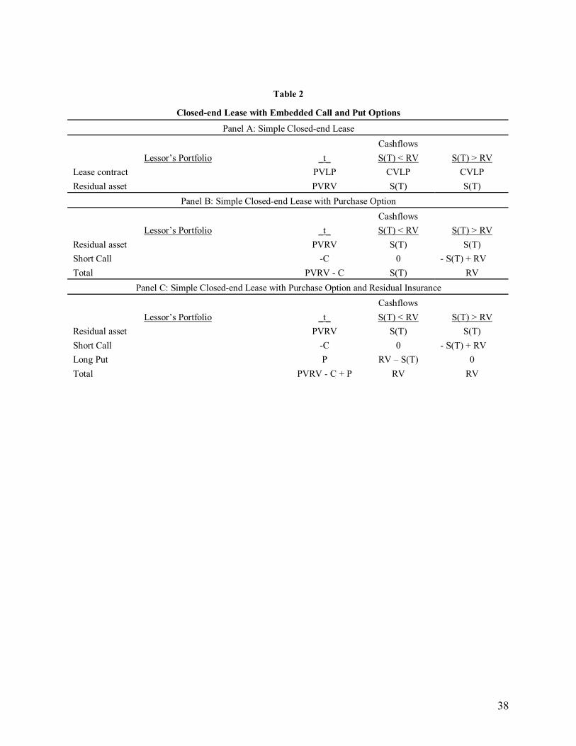
38

Table 2

Closed-end Lease with Embedded Call and Put Options

Panel A: Simple Closed-end Lease Cashflows

Lessor�s Portfolio _t_ S(T) < RV S(T) > RV Lease contract PVLP CVLP CVLP Residual asset PVRV S(T) S(T)

Panel B: Simple Closed-end Lease with Purchase Option Cashflows

Lessor�s Portfolio _t_ S(T) < RV S(T) > RV Residual asset PVRV S(T) S(T) Short Call -C 0 - S(T) + RV Total PVRV - C S(T) RV

Panel C: Simple Closed-end Lease with Purchase Option and Residual Insurance Cashflows

Lessor�s Portfolio _t_ S(T) < RV S(T) > RV Residual asset PVRV S(T) S(T) Short Call -C 0 - S(T) + RV Long Put P RV � S(T) 0 Total PVRV - C + P RV RV

39

Table 3

Summary Statistics on Used Car Prices

This table reports on the distribution of monthly NADA used car prices for T-year-old (T = 2, 3, 4, and 5) used cars

of constant quality for the sample period November 1990 through November 2006. The sample period includes car

model years 1990 through 2006. The price series for Saturn begins April 1992, with its 1991 model year. All

prices are averages from reporting automobile dealers. For each T, reported statistics are mean and standard

deviation (SD) in the first row, and (median) and (number of monthly observations (N)) in the second row. Panel A: Wholesale Prices

Model T = 2 T = 3 T = 4 T = 5 Total Mean SD Mean SD Mean SD Mean SD Mean SD (Median) (N) (Median) (N) (Median) (N) (Median) (N) (Median) (N)

All 9963 1594 8735 1541 7439 1435 6090 1197 8179 2049 (9700) (531) (8575) (495) (7275) (459) (6125) (423) (8150) (1908) Camry 11605 940 10247 990 8819 922 7208 659 9605 1856 (11700) (181) (10450) (169) (8925) (157) (7250) (145) (9563) (652) Civic 9563 987 8482 888 7302 831 6082 644 7964 1551 (9600) (181) (8525) (169) (7225) (157) (5925) (145) (8013) (652) Saturn 8634 1082 7379 1102 6094 982 4880 896 6871 1733 (8975) (169) (7875) (157) (6300) (145) (4850) (133) (6938) (604)

Panel B: Estimates of Annual Standard Deviations

This Panel presents standard deviations (SD) of percentage price changes in the NADA used car price series based

on overlapping monthly observations for the full data set covering November 1990 through November 2006; T

represents the lease term in years, and N denotes the number of monthly observations.

Model T = 2 T = 3 T = 4 T = 5 Total N SD N SD N SD N SD N SD All 495 0.0842 459 0.0989 423 0.0985 387 0.1093 1764 0.0974 Camry 169 0.0530 157 0.0855 145 0.0917 133 0.0904 604 0.0805 Civic 169 0.0475 157 0.0548 145 0.0726 133 0.0784 604 0.0634 Saturn 157 0.1291 145 0.1400 133 0.1198 121 0.1416 556 0.1334

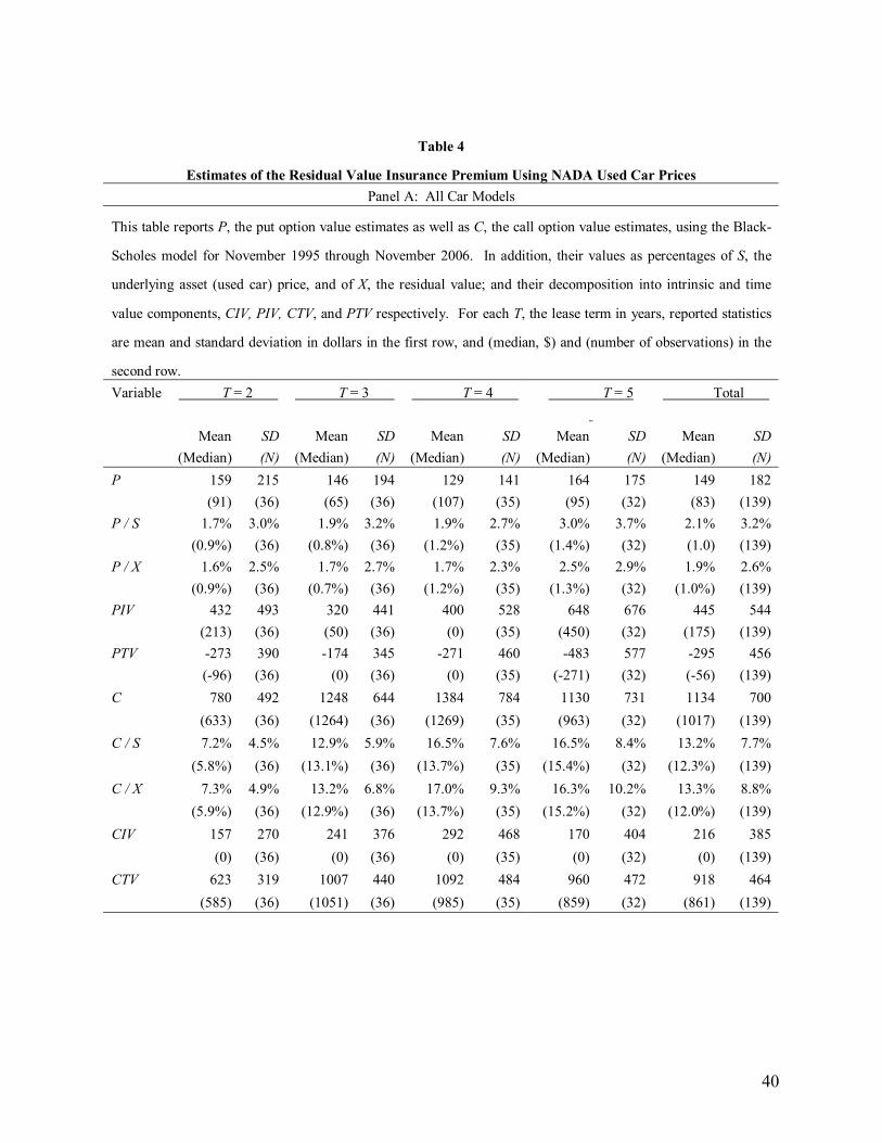
40

Table 4

Estimates of the Residual Value Insurance Premium Using NADA Used Car Prices Panel A: All Car Models

This table reports P, the put option value estimates as well as C, the call option value estimates, using the Black-

Scholes model for November 1995 through November 2006. In addition, their values as percentages of S, the

underlying asset (used car) price, and of X, the residual value; and their decomposition into intrinsic and time

value components, CIV, PIV, CTV, and PTV respectively. For each T, the lease term in years, reported statistics

are mean and standard deviation in dollars in the first row, and (median, $) and (number of observations) in the

second row. Variable T = 2 T = 3 T = 4 T = 5

Total

Mean SD Mean SD Mean SD Mean SD Mean SD (Median) (N) (Median) (N) (Median) (N) (Median) (N) (Median) (N)P 159 215 146 194 129 141 164 175 149 182 (91) (36) (65) (36) (107) (35) (95) (32) (83) (139) P / S 1.7% 3.0% 1.9% 3.2% 1.9% 2.7% 3.0% 3.7% 2.1% 3.2% (0.9%) (36) (0.8%) (36) (1.2%) (35) (1.4%) (32) (1.0) (139) P / X 1.6% 2.5% 1.7% 2.7% 1.7% 2.3% 2.5% 2.9% 1.9% 2.6% (0.9%) (36) (0.7%) (36) (1.2%) (35) (1.3%) (32) (1.0%) (139) PIV 432 493 320 441 400 528 648 676 445 544 (213) (36) (50) (36) (0) (35) (450) (32) (175) (139) PTV -273 390 -174 345 -271 460 -483 577 -295 456 (-96) (36) (0) (36) (0) (35) (-271) (32) (-56) (139) C 780 492 1248 644 1384 784 1130 731 1134 700 (633) (36) (1264) (36) (1269) (35) (963) (32) (1017) (139) C / S 7.2% 4.5% 12.9% 5.9% 16.5% 7.6% 16.5% 8.4% 13.2% 7.7% (5.8%) (36) (13.1%) (36) (13.7%) (35) (15.4%) (32) (12.3%) (139) C / X 7.3% 4.9% 13.2% 6.8% 17.0% 9.3% 16.3% 10.2% 13.3% 8.8% (5.9%) (36) (12.9%) (36) (13.7%) (35) (15.2%) (32) (12.0%) (139) CIV 157 270 241 376 292 468 170 404 216 385 (0) (36) (0) (36) (0) (35) (0) (32) (0) (139) CTV 623 319 1007 440 1092 484 960 472 918 464 (585) (36) (1051) (36) (985) (35) (859) (32) (861) (139)

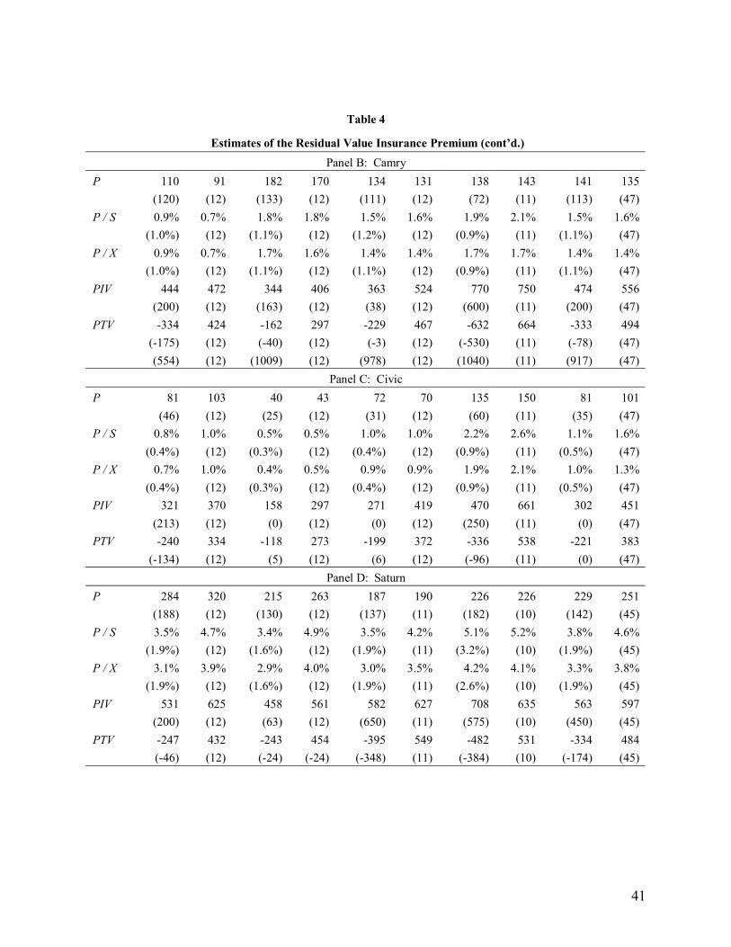
41

Table 4

Estimates of the Residual Value Insurance Premium (cont�d.) Panel B: Camry

P 110 91 182 170 134 131 138 143 141 135 (120) (12) (133) (12) (111) (12) (72) (11) (113) (47) P / S 0.9% 0.7% 1.8% 1.8% 1.5% 1.6% 1.9% 2.1% 1.5% 1.6% (1.0%) (12) (1.1%) (12) (1.2%) (12) (0.9%) (11) (1.1%) (47) P / X 0.9% 0.7% 1.7% 1.6% 1.4% 1.4% 1.7% 1.7% 1.4% 1.4% (1.0%) (12) (1.1%) (12) (1.1%) (12) (0.9%) (11) (1.1%) (47) PIV 444 472 344 406 363 524 770 750 474 556 (200) (12) (163) (12) (38) (12) (600) (11) (200) (47) PTV -334 424 -162 297 -229 467 -632 664 -333 494 (-175) (12) (-40) (12) (-3) (12) (-530) (11) (-78) (47) (554) (12) (1009) (12) (978) (12) (1040) (11) (917) (47)

Panel C: Civic P 81 103 40 43 72 70 135 150 81 101 (46) (12) (25) (12) (31) (12) (60) (11) (35) (47) P / S 0.8% 1.0% 0.5% 0.5% 1.0% 1.0% 2.2% 2.6% 1.1% 1.6% (0.4%) (12) (0.3%) (12) (0.4%) (12) (0.9%) (11) (0.5%) (47) P / X 0.7% 1.0% 0.4% 0.5% 0.9% 0.9% 1.9% 2.1% 1.0% 1.3% (0.4%) (12) (0.3%) (12) (0.4%) (12) (0.9%) (11) (0.5%) (47) PIV 321 370 158 297 271 419 470 661 302 451 (213) (12) (0) (12) (0) (12) (250) (11) (0) (47) PTV -240 334 -118 273 -199 372 -336 538 -221 383 (-134) (12) (5) (12) (6) (12) (-96) (11) (0) (47)

Panel D: Saturn P 284 320 215 263 187 190 226 226 229 251 (188) (12) (130) (12) (137) (11) (182) (10) (142) (45) P / S 3.5% 4.7% 3.4% 4.9% 3.5% 4.2% 5.1% 5.2% 3.8% 4.6% (1.9%) (12) (1.6%) (12) (1.9%) (11) (3.2%) (10) (1.9%) (45) P / X 3.1% 3.9% 2.9% 4.0% 3.0% 3.5% 4.2% 4.1% 3.3% 3.8% (1.9%) (12) (1.6%) (12) (1.9%) (11) (2.6%) (10) (1.9%) (45) PIV 531 625 458 561 582 627 708 635 563 597 (200) (12) (63) (12) (650) (11) (575) (10) (450) (45) PTV -247 432 -243 454 -395 549 -482 531 -334 484 (-46) (12) (-24) (-24) (-348) (11) (-384) (10) (-174) (45)

42

Table 5

Estimates of the Residual Value Insurance Premiums Using ALG Used Car Prices

Panel A reports summary statistics on residual values obtained from ALG for November 1995 through November

2006. For each T, the lease term in years, reported statistics are mean and standard deviation in dollars in the first

row and (median, $) and (number of observations) in the second row. Panel B presents annual standard

deviations (SD) of percentage changes in the ALG used car price series; N stands for number of observations.

Panel C reports summary statistics on put options estimates across all car types. Panel A: Residual Values

Model T = 2 T = 3 T = 4 T = 5 Total Mean SD Mean SD Mean SD Mean SD Mean SD (Median) (N) (Median) (N) (Median) (N) (Median) (N) (Median) (N)

All 10918 1679 9424 1509 8128 1398 7060 1330 8883 2063 (10713) (36) (9200) (36) (8013) (36) (7038) (36) (8775) (144) Camry 12710 681 11031 695 9542 823 8296 957 10395 1838 (12763) (12) (10988) (12) (9338) (12) (8200) (12) (10400) (48) Civic 10600 939 9197 634 7954 441 6919 404 8663 1521 (10288) (12) (8950) (12) (7825) (12) (6875) (12) (8700) (48) Saturn 9444 1281 8063 1206 6890 1209 5967 1248 7591 1779 (9513) (12) (8025) (12) (6763) (12) (5863) (12) (7613) (48)

Panel B: Standard Deviations Model T = 2 T = 3 T = 4 T = 5 Total N SD N SD N SD N SD N SDAll 36 0.0695 36 0.0716 36 0.0831 36 0.1102 144 0.0836 Camry 12 0.0513 12 0.0545 12 0.0603 12 0.0804 48 0.0616 Civic 12 0.0575 12 0.0583 12 0.0710 12 0.0927 48 0.0699 Saturn 12 0.0999 12 0.1022 12 0.1179 12 0.1574 48 0.1193

Panel C: Put Premiums Variable T = 2 T = 3 T = 4 T = 5 Total Mean SD Mean SD Mean SD Mean SD Mean SD (Median) (N) (Median) (N) (Median) (N) (Median) (N) (Median) (N)

P 122 89 93 77 96 78 145 105 114 90 (127) (36) (89) (36) (82) (36) (114) (36) (100) (144) P / X 1.2% 1.1% 1.1% 1.1% 1.4% 1.3% 2.4% 2.1% 1.5% 1.5% (1.2%) (36) (0.9%) (36) (1.0%) (36) (1.6%) (36) (1.2%) (144)

43

Table 6

Estimates of the Value of Residual Value Insurance Using Used Car Price Index

These Panels report the results of using the CPI Used Car component to determine changes in the price level of used

cars. For each T the lease term in years, reported statistics are mean and standard deviation in dollars in the first

row, and (median, $) and (number of observations) in the second row.

Variable T = 2 T = 3 T = 4 T = 5 Total Mean SD Mean SD Mean SD Mean SD Mean SD Median N Median N Median N Median N Median N

Panel A: Used Car Index and Exercise Prices

This panel reports on the distribution of used car prices, S, for T -year-old (T = 2, 3, 4, and 5) used cars for the

sample period January 1953 through November 2006. Panel A also reports summary statistics on residual values, X,

obtained from ALG for November 1995 through November 2006 used in conjunction with NADA used car values to

determine a ratio, X/S, to be applied to the CPI-generated prices.

S 9630 629 8698 568 7757 507 6449 421 8133 1298 (9794) (12) (8846) (12) (7889) (12) (6558) (12) (8166) (48) X 9887 842 8789 760 7904 893 6984 941 8391 1369 (9947) (12) (8916) (12) (7822) (12) (6968) (12) (8429) (48)

Panel B: Estimates of Residual Value Insurance Premium

This panel reports P, the put option value estimates using the Black-Scholes model; its value as percentages of S, the

underlying asset (used car) price, and of X, the residual value. Also shown is its decomposition into intrinsic and

time value components, PIV and PTV, for November 1995 through November 2006. P 383 183 288 177 252 164 274 171 299 176 (369) (12) (247) (12) (243) (12) (217) (12) (259) (48) P / S 4.0% 2.1% 3.4% 2.3% 3.3% 2.3% 4.3% 2.8% 3.8% 2.3% (3.7%) (12) (2.8%) (12) (3.0%) (12) (3.5%) (12) (3.2%) (48) P / X 3.9% 1.9% 3.3% 2.1% 3.1% 2.1% 3.8% 2.2% 3.5% 2.0% (3.6%) (12) (2.9%) (12) (2.9%) (12) (3.3%) (12) (3.1%) (48) PIV 349 420 258 376 351 514 605 661 391 506 (99) (12) (0) (12) (47) (12) (397) (12) (111) (48) PTV 34 317 30 313 -99 429 -331 545 -92 426 (181) (12) (119) (12) (76) (12) (-174) (12) (85) (48)

44

Table 7

Sensitivity Analyses of the Value of Residual Value Insurance based on NADA Used Car Prices

This table presents average sensitivities of put prices across the three car brands to the five input variables, the

underlying asset (used car) price (S), the exercise price (X), the standard deviation, the risk-free rate, and time.

Specifically, the reported sensitivities are the change in put price in response to a unit change in the price of the

underlying asset, Delta (∂P/∂S); change in the exercise price, ∂P/∂X; change in the volatility of used car price

change, Vega; change in the risk-free rate, Rho; change in time, Theta; and the change in Delta in response to a unit

change in the underlying asset price, Gamma. For each T, the lease term in years, reported statistics are mean and

standard deviation in the first row, and (median) and (number of observations) in the second row. Variable T = 2 T = 3 T = 4 T = 5 Total

Mean SD Mean SD Mean SD Mean SD Mean SD (Median) (N) (Median) (N) (Median) (N) (Median) (N) (Median) (N)

Delta -0.24 0.23 -0.18 0.19 -0.17 0.16 -0.21 0.18 -0.20 0.19 (-0.19) (36) (-0.13) (36) (-0.16) (35) (-0.17) (32) (-0.17) (139)∂P / ∂X 0.24 0.22 0.18 0.19 0.17 0.16 0.21 0.17 0.16 0.18 (0.20) (36) (0.14) (36) (0.17) (35) (0.16) (32) (0.16) (139)Vega 3455 2203 3159 1988 3035 1942 3216 1776 3218 1974 (3721) (36) (2878) (36) (3221) (35) (3134) (32) (3221) (139)Rho -5194 4376 -5013 4537 -5323 4409 -7040 5521 -5605 4727 (-4073) (36) (-3475) (36) (-5851) (35) (-5907) (32) (-4576) (139)Theta 56 85 28 36 27 34 37 41 37 55 (19) (36) (16) (36) (13) (35) (15) (32) (15) (139)

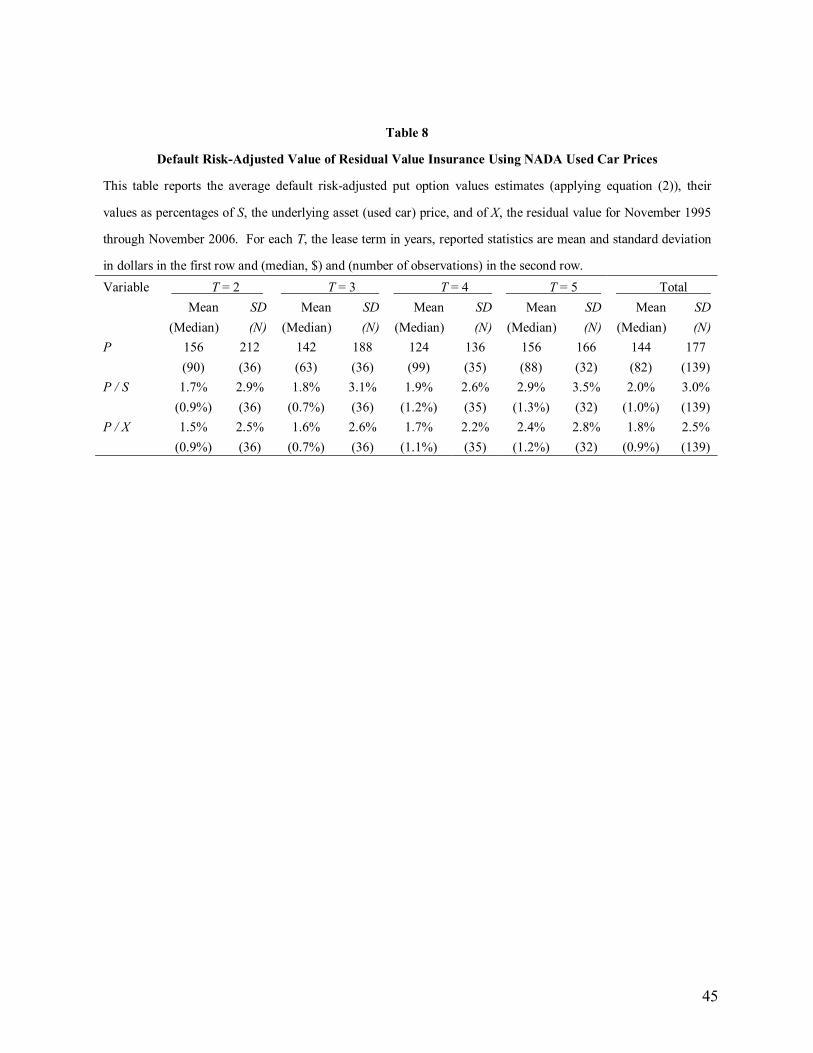
45

Table 8

Default Risk-Adjusted Value of Residual Value Insurance Using NADA Used Car Prices

This table reports the average default risk-adjusted put option values estimates (applying equation (2)), their

values as percentages of S, the underlying asset (used car) price, and of X, the residual value for November 1995

through November 2006. For each T, the lease term in years, reported statistics are mean and standard deviation

in dollars in the first row and (median, $) and (number of observations) in the second row. Variable T = 2 T = 3 T = 4 T = 5 Total

Mean SD Mean SD Mean SD Mean SD Mean SD (Median) (N) (Median) (N) (Median) (N) (Median) (N) (Median) (N)

P 156 212 142 188 124 136 156 166 144 177 (90) (36) (63) (36) (99) (35) (88) (32) (82) (139) P / S 1.7% 2.9% 1.8% 3.1% 1.9% 2.6% 2.9% 3.5% 2.0% 3.0% (0.9%) (36) (0.7%) (36) (1.2%) (35) (1.3%) (32) (1.0%) (139) P / X 1.5% 2.5% 1.6% 2.6% 1.7% 2.2% 2.4% 2.8% 1.8% 2.5% (0.9%) (36) (0.7%) (36) (1.1%) (35) (1.2%) (32) (0.9%) (139)

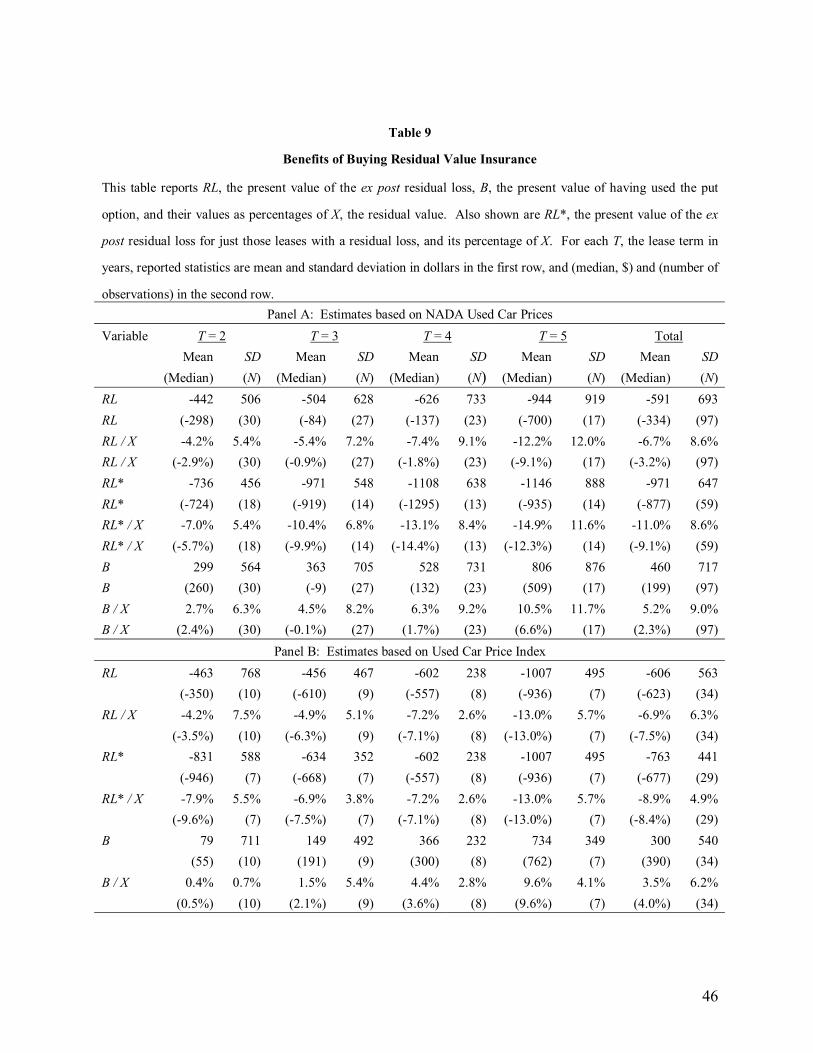
46

Table 9

Benefits of Buying Residual Value Insurance

This table reports RL, the present value of the ex post residual loss, B, the present value of having used the put

option, and their values as percentages of X, the residual value. Also shown are RL*, the present value of the ex

post residual loss for just those leases with a residual loss, and its percentage of X. For each T, the lease term in

years, reported statistics are mean and standard deviation in dollars in the first row, and (median, $) and (number of

observations) in the second row. Panel A: Estimates based on NADA Used Car Prices

Variable T = 2 T = 3 T = 4 T = 5 Total Mean SD Mean SD Mean SD Mean SD Mean SD (Median) (N) (Median) (N) (Median) (N) (Median) (N) (Median) (N) RL -442 506 -504 628 -626 733 -944 919 -591 693 RL (-298) (30) (-84) (27) (-137) (23) (-700) (17) (-334) (97) RL / X -4.2% 5.4% -5.4% 7.2% -7.4% 9.1% -12.2% 12.0% -6.7% 8.6% RL / X (-2.9%) (30) (-0.9%) (27) (-1.8%) (23) (-9.1%) (17) (-3.2%) (97) RL* -736 456 -971 548 -1108 638 -1146 888 -971 647 RL* (-724) (18) (-919) (14) (-1295) (13) (-935) (14) (-877) (59) RL* / X -7.0% 5.4% -10.4% 6.8% -13.1% 8.4% -14.9% 11.6% -11.0% 8.6% RL* / X (-5.7%) (18) (-9.9%) (14) (-14.4%) (13) (-12.3%) (14) (-9.1%) (59) B 299 564 363 705 528 731 806 876 460 717 B (260) (30) (-9) (27) (132) (23) (509) (17) (199) (97) B / X 2.7% 6.3% 4.5% 8.2% 6.3% 9.2% 10.5% 11.7% 5.2% 9.0% B / X (2.4%) (30) (-0.1%) (27) (1.7%) (23) (6.6%) (17) (2.3%) (97)

Panel B: Estimates based on Used Car Price Index RL -463 768 -456 467 -602 238 -1007 495 -606 563 (-350) (10) (-610) (9) (-557) (8) (-936) (7) (-623) (34) RL / X -4.2% 7.5% -4.9% 5.1% -7.2% 2.6% -13.0% 5.7% -6.9% 6.3% (-3.5%) (10) (-6.3%) (9) (-7.1%) (8) (-13.0%) (7) (-7.5%) (34) RL* -831 588 -634 352 -602 238 -1007 495 -763 441 (-946) (7) (-668) (7) (-557) (8) (-936) (7) (-677) (29) RL* / X -7.9% 5.5% -6.9% 3.8% -7.2% 2.6% -13.0% 5.7% -8.9% 4.9% (-9.6%) (7) (-7.5%) (7) (-7.1%) (8) (-13.0%) (7) (-8.4%) (29) B 79 711 149 492 366 232 734 349 300 540 (55) (10) (191) (9) (300) (8) (762) (7) (390) (34) B / X 0.4% 0.7% 1.5% 5.4% 4.4% 2.8% 9.6% 4.1% 3.5% 6.2% (0.5%) (10) (2.1%) (9) (3.6%) (8) (9.6%) (7) (4.0%) (34)

47

Table 10

Subvention at 110% of ALG Residual Value - Benefits of Buying Insurance

This table reports RL, the present value of the ex post residual loss based on NADA Used Car prices over all car

models, B, the present value of having used the put option, and their values as percentages of X, the residual value

when X is 110% of the ALG value. Also shown are RL*, the present value of the ex post residual loss for just those

leases with a residual loss, and its percentage of X. For each T, the lease term in years, reported statistics are mean

and standard deviation in dollars in the first row, and (median, $) and (number of observations) in the second row.

Variable T = 2 T = 3 T = 4 T = 5 Total Mean SD Mean SD Mean SD Mean SD Mean SD (Median) (N) (Median) (N) (Median) (N) (Median) (N) (Median) (N) RL -1121 864 -1037 913 -1121 947 -1417 1084 -1150 932 RL (-1299) (30) (-890) (27) (-814) (23) (-1267) (17) (-1155) (97) RL / X -9.4% 7.7% -9.9% 9.0% -12.0% 10.3% -16.8% 12.5% -11.5% 9.9% RL / X (-10.9%) (30) (-8.4%) (27) (-8.8%) (23) (-15.0%) (17) (-11.0%) (97) RL* -1463 680 -1333 818 -1433 829 -1721 939 -1467 800 RL* (-1445) (23) (-1464) (21) (-1502) (18) (-1468) (14) (-1454) (76) RL* / X -12.2% 6.4% -12.8% 8.2% -15.3% 9.1% -20.4% 10.6% -14.6% 8.8% RL* / X (-12.1%) (23) (-14.0%) (21) (-14.0%) (18) (-17.9%) (14) (-14.0%) (76) B 520 1000 623 1100 837 949 1083 956 723 1015 B (672) (30) (513) (27) (702) (23) (800) (17) (679) (97) B / X 4.2% 9.7% 5.9% 11.4% 9.0% 10.7% 12.9% 11.5% 7.3% 11.1% B / X (5.4%) (30) (5.0%) (27) (8.4%) (23) (9.4%) (17) (6.2%) (97)

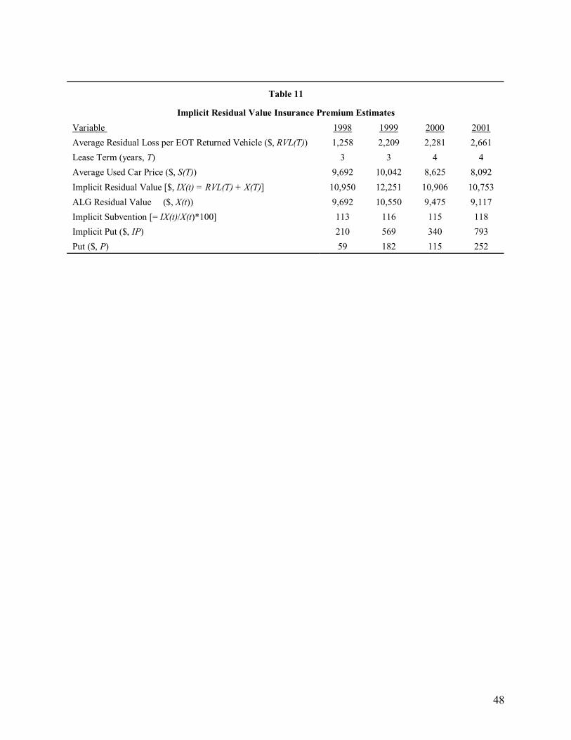
48

Table 11

Implicit Residual Value Insurance Premium Estimates Variable 1998 1999 2000 2001 Average Residual Loss per EOT Returned Vehicle ($, RVL(T)) 1,258 2,209 2,281 2,661 Lease Term (years, T) 3 3 4 4 Average Used Car Price ($, S(T)) 9,692 10,042 8,625 8,092 Implicit Residual Value [$, IX(t) = RVL(T) + X(T)] 10,950 12,251 10,906 10,753 ALG Residual Value ($, X(t)) 9,692 10,550 9,475 9,117 Implicit Subvention [= IX(t)/X(t)*100] 113 116 115 118 Implicit Put ($, IP) 210 569 340 793 Put ($, P) 59 182 115 252

49

References

Akerlof, George A., 1970, The market for �lemons�: Quality uncertainty and the market

mechanism, Quarterly Journal of Economics 84, 488-500.

American Financial Group, 2006, www.afginc.com.

American Honda Finance Corporation, 1999, Honda Auto Lease Trust 1999-A Prospectus.

Angel, James J., 1997, Leasing: Chrysler Corporation 1995, Working paper, Georgetown

University.

Association of Consumer Vehicle Lessors, www.acvl.com.

Astorina, Joseph J., and Chris Mrazek, 2000, Under the hood: Automobile lease ABS

uncovered, www.fitchratings.com.

Black, Fischer, and Myron Scholes, 1973, The pricing of options and corporate liabilities,

Journal of Political Economy 81, 637-659.

Eisfeldt, Andrea L., and Adriano A. Rampini, 2008, Leasing, ability to repossess, and debt

capacity, Review of Financial Studies, 1-37.

http://www.leasefoundation.org/IndRsrcs/MrktOvrvws/SOI08.htm.

Giaccotto, Carmelo, Gerson M. Goldberg, and Shantaram P. Hegde, 2007, The value of

embedded real options: Evidence from consumer automobile lease contracts, Journal of Finance

62, 411-445.

Grenadier, Steven R., 1995, Valuing lease contracts: A real-options approach, Journal of

Financial Economics 38, 297-331.

50

Grenadier, Steven R., 1996, Leasing and credit risk, Journal of Financial Economics 42, 33-364.

Hendel, Igal, and Alessandro Lizzeri, 1999, Adverse selection in durable good markets,

American Economic Review 89, 1097-1115.

Hendel, Igal, and Alessandro Lizzeri, 2002, The role of leasing under adverse selection, Journal

of Political Economy 110, 113-143.

Hull, John, and Alan White, 1995, The impact of default risk on the prices of options and other

derivative securities, Journal of Banking and Finance 19, 299-322.

Ibbotson Associates, 2000, Stocks, Bonds, Bills, and Inflation, (Chicago, Illinois).

Jarrow, Robert A., and Stuart M. Turnbull, 1995, Pricing derivatives on financial securities

subject to credit risk, Journal of Finance 50, 53-85.

International Business Machines Corporation and Subsidiary Companies, Annual Reports.

Kay, John, 2005, Introduce professional standards for senior bankers, Financial Times, February

18, 2009, p.11.

Kolber, Vincent A., 1985, Residual value insurance: A Risk management tool for the leasing

industry,� Journal of Equipment Lease Financing 3, 1-10.

Kravitt, Jason H. P., and Elizabeth A. Raymond, 1995, Overcoming the legal barriers to auto

lease securitization, www.securitization.net.

McConnell, John J., and James S. Schallheim, 1983, Valuation of asset leasing contracts, Journal

of Financial Economics 12, 237-261.

Merton, Robert C., 1974, On the pricing of corporate debt: The risk structure of interest rates,

Journal of Finance 29, 449-470.

51

Moel, Alberto, and Peter Tufano, 2002, When are real options exercised? An empirical study of

mine closings, Review of Financial Studies 15, 35-64.

www.moodys.com

Pashigian, B. Peter, 2001, The used car price index: A checkup and suggested repairs, Working

paper, Bureau of Labor Statistics.

Pashigian, B. Peter, Brian Bowen, and Eric Gould, 1995, Fashion, styling, and the within-season

decline in automobile prices, Journal of Law and Economics 38, 281-310.

Quigg, Laura, 1993, Empirical testing of real option-pricing models, Journal of Finance 48, 621-

640.

www.fitchratings.com, R.V.I. Guaranty Co., Ltd. and R.V.I. America Insurance Co.

RatingsDirect, 2006, R.V.I. Guaranty Co. Ltd., www.standardandpoors.com.

Schallheim, James S., and John J. McConnell, 1985, A model for the determination of the �fair�

premiums on lease cancellation insurance policies, Journal of Finance 40, 1439-1457.

Scism, Leslie, 2009, Added value � and anxiety � for variable-annuity owners, The Wall Street

Journal, February 2.

Smith Clifford W., Jr., and L. MacDonald Wakeman, 1985, Determinants of corporate leasing

policy, Journal of Finance 40, 895-908.

Vertex Consultants Inc., 1998, Bank participation in U.S. retail automobile leasing: An

overview Toronto, http://www.fin.gc.ca/taskforce/pdf/cba11.pdf

Waldman, Michael, 1997, Eliminating the market for secondhand goods: an alternative

explanation for leasing, Journal of Law and Economics 40, 61-92.

52

Walsh, Mary Williams, 2008, Life insurers facing cuts in ratings, New York Times,

nytimes.com.

Wolfe, Christopher D., Thomas J. Abruzzo, John S. Olert, and Marvin G. Behm, 2001, Auto

finance 2000: Review and outlook, www.fitchratings.com.

53

Endnotes

1. See �Chrysler Retreat on Leases. Move Could Dent Sales; Resale Values Dive�, The

Wall Street Journal, July 26-27, 2008. It also reported that Ford Motor Co. took a write-

down of $2.1 billion related to unprofitable lease deals made by Ford Motor Credit.

2. The 2008 industry future council report by the Equipment Leasing and Finance

Association (ELFA) estimates that the market size for equipment/asset acquisition is $1.3

trillion of which $600 billion is leased or financed. It also notes that over 80% of

American businesses lease at least one of their equipment acquisitions.

Based on the 1992 Census of Manufacturers microdata, Eisfeldt and Rampini (2008)

report that the fraction of leased capital invested in buildings, structures, and equipment,

defined as the ratio of operating lease payments to an estimate of the user cost of owned

capital (which is the sum of the interest cost on the owned capital and depreciation) is

about 16% on average (median of 12%).

3. In essence, the lease security has fixed monthly cashflows covering (a) expected

depreciation on the real asset and interest charge on capital invested, and (b) an uncertain

cashflow at maturity tied to the future value of the underlying real asset. In the structured

finance literature, this type of claim is called an equity (or asset)-linked bond � a bond

that pays fixed cash coupons at periodic intervals and a share of stock (a unit of an

asset)at maturity.

4. Thus, for instance, many construction and manufacturing equipment leases cover terms

up to ten years with relatively small residual values.

5. For example, the 10-K of The Hartford Financial Services Group, Inc. reports: �On June

30, 2003, the Company entered into a sale-leaseback of certain furniture and fixtures with

a net book value of $40 million. The sale-leaseback resulted in a gain of $15 million,

54

which was deferred and will be amortized into earnings over the initial lease term of three

years. The lease qualifies as an operating lease for accounting purposes. At the end of

the initial lease term, the Company has the option to purchase the leased assets, renew the

lease for two one-year periods, or return the leased assets to the lessor. If the Company

elects to return the assets to the lessor at the end of the initial lease term, the assets will be

sold, and the Company has guaranteed a residual value on the furniture and fixtures of

$20 million. If the fair value of the furniture and fixtures were to decline below the

residual value, the Company would have to make up the difference under the residual

value guarantee.� http://www.sec.gov/Archives/edgar/data

6. A long position in the underlying asset combined with a long put and a short call (with

both identical strike price and term to maturity equal to that of a forward contract on the

underlying) is known as a collar. Since we make the assumption that the strike price (i.e.,

residual value) and the term to expiration of the two options are identical to that of a

forward contract on the equipment, put and call options are equal in value, thus resulting

in a zero-cost collar. In this setting, the lessee holds a short bond position with a value

equal to the present value of lease payments and a long forward position on the residual

asset.

7. In contrast, in a vehicle lease for commercial fleets (called TRAC � Terminal Rental

Adjustment Clause) the lessee guarantees the residual value.

8. Another widely used method of classifying lease contracts focuses on the proportion of

the original cost of equipment recovered thorough lease payments, called the 90-10 test.

A lease is termed as an operating (or true) lease under financial accounting standards

(FAS 13 and IAS 17) if the present value of lease payments plus any third-party-

guaranteed portion of the residual value is no more than 90% of the equipment�s capital

cost, implying that the lessor retains at least 10% of residual value. By contrast, in a

55

financial or capital lease the lessor reclaims at least 90% of the equipment�s capital cost

through lease cashflows and residual value insurance.

9. For the captive leasing companies, the higher residuals also allow the parent automaker to

increase sales volume.

10. Recently some industry analysts have proclaimed that the persistent willingness of

captives to enhance residuals coupled with their lack of diversification and the recent

dramatic short-term run up in fuel prices have all conspired against them to create a truly

perfect storm against the captive lessors, see GMAC Dramatically Cut Back on Leases in

September, October 6, 2008. http://www.nvlalifeline.com/News.cfm?id=1102.

11. Weighted average residual losses declined to $2,909 in 2003. The new lease volume

peaked in 1999 at 3.2 million vehicles but fell to 1.62 million in 2003 and increased

slightly to1.69 million in 2004. In 1998, the EOT return rate for medium lessors held

constant for another year, but the return rate for large lessors jumped from 46% to 54%. 12. In a broad sense, these early terminations are comparable to short sales, which are at

times used as alternatives to foreclosures in real estate /mortgage finance. In a short sale,

a mortgage lender allows the homeowner in financial distress (i.e., the borrower owes

more than the home is worth (with negative equity)) to sell the house for less than the

value of the outstanding loan and forgives the difference. The lender approves the short

sale because he tends to lose less on the sale than if a home fell into foreclosure.

13. See R.V.I. Guaranty Co. Ltd., RatingsDirect, www.standardandpoors.com, Jan. 07, 2006.

R.V.I. group (consisting of R.V.I. Guaranty Co. Ltd. and R.V.I. America Insurance Co.)

is the market leader in the residual value insurance sector with a total gross premium in

force in 2004 of $234 million on an insured portfolio with a maximum liability of $14

56

billion. Its 2004 portfolio covers four main asset classes: passenger vehicles (with an

average policy term of one to five years accounting for 68% of maximum insurance

liability), real estate (20 years, 12%) and commercial equipment and aircraft (eight to ten

years, 20%). The average term across all segments is about nine years. Its clients are

drawn from captive financing arms of auto manufacturers, bank lessors, independent fleet

/ leasing companies, credit unions, and investors in vehicle lease-backed securitizations.

R.V.I.�s portfolio is representative of the residual value insurance industry. Coverage of

leased vehicles (both individual vehicle and fleet policies) is the most common segment,

as compared with equipment leasing.

14. Residual value insurance or guarantee offers several other benefits. In the durable asset

market, guaranteeing the future value may help the manufacturer bring about a sale.

However, residual value guarantee by the vendor may result in the transaction being

accounted for as a lease. If the lease transaction is supported by a third-party RVI a,

financial accounting standards (FAS 13 and IAS�17) allow lessors to recognize the

transaction as a sale for accounting purposes, accelerate recognition of lease income and

permit off-balance-sheet accounting for asset securitization. Specifically, if the present

value of lease payments and the third-party guarantee of the residual value exceed 90% of

the value of the asset at the inception of the lease, a lessor may classify a lease as a

financial lease.

In addition, purchasing RVI generates other benefits such as improved loan-to-value

ratios, expanded funding sources, and securitization of lease portfolios under which

bonds backed by the residual value (resale value) of leased vehicles are sold to investors.

In the real estate market, lenders often require RVI when high leverage is used to

purchase a property. In such a transaction, the loan does not fully amortize during its

term, thus exposing the lender to the risk that the large final payment (balloon) will not

57

be fully collateralized by the underlying asset. The purchase of RVI serves to guarantee

that the asset value will be sufficient to collateralize the balloon payment. For more

details, see R.V.I. Guaranty Co., Ltd. and R.V.I. America Insurance Co. at

www.fitchratings.com.

15. For instance, in 2006 The Specialty Financial group, a unit of American Financial Group,

reported underwriting losses attributable to the automobile residual value business, driven

primarily by lower than expected proceeds from the sale (at auction) of certain luxury

cars and sport utility vehicles, www.afginc.com.

16. Unlike conventional insurance, such as life, health, property and casualty, where insured

risks tend to be independent, residual value risk is correlated across insured assets � when

residual values go down, they all go down together. Given the small size of the residual

value premium, about 2% to 5% of the insured amount, a few large losses could threaten

the survival of the insurer.

Broadly, minimum security price or return guarantees are often/widely offered in the

financial services industry to gain market share. For instance, The Hartford Financial

Services Group is a market leader in guarantees of minimum withdrawal of benefits from

variable annuity life insurance policies, regardless of how the underlying investment

portfolio performs. It suffered huge losses on annuity guarantees in the recent global

financial turmoil, leading some analysts to comment that the life insurer significantly

underpriced the guarantees. Managing growing risk exposures inherent in such hidden

embedded options has emerged as one of the most significant risk management

challenges confronting the financial services industry, see Walsh (2008).

17 . For instance, Kay (2009) observes that bank executives on average tend to lack the range

of abilities required to understand the advanced structured products and the assumptions,

structure, strengths and limitations of the numerous quantitative risk management models

58

that rule the modern financial system. Conventional professional qualifications in the

financial services industry lack the rigorous training and examination necessary to

understand these complex products leading to the current loss of public trust and

confidence in the financial services industry. 18 . See Scism (2009).

19. See McConnell and Schallheim (1983) for a model on the valuation of lease payments

with embedded options and Grenadier (1996) for equilibrium determination of residual

value insurance premiums.

20. Put differently, the lessee in the open-ended lease owns a forward contract on the residual

asset (in addition to the lease obligations). An important difference is that in the closed-

end auto lease, an insurance firm provides protection against residual value risk, but in

the open-ended equipment lease, the lessee offers the residual value guarantee. For

example, Global Financing, a subsidiary of International Business Machines Corp,

manages residual value risk by optimizing recovery of residual values. It does this

through extending lease arrangements with current clients, leasing used equipment to new

clients, selling assets sourced from end of lease, and, on a limited basis, obtaining third-

party guarantees of the future value of the equipment to be returned at end of lease. It

purchased guarantees for residual values of $27 million and $36 million associated with

capital costs of $651 million and $700 million of financing transactions originated during

2005 and 2004, respectively. The cost of these guarantees was $4.3 million for 2005, and

$5.7 million for 2004, which amount to about 16% of insured value, see International

Business Machines Corporation and Subsidiary Companies (2005).

21. In practice, several factors tend to render the cancellation option worthless. Contrary to

the theoretical models, the lessee is typically not allowed to buy the cancellation option at

the time of signing the contract, and the penalty imposed upon cancellation completely

59

offsets the gain due to the drop in the market value of the leased automobile. As noted

earlier, historical evidence on early terminations is predominantly attributable to the

aggressive marketing strategy of using unduly high residual values to lower monthly

lease payments (see Astorina and Mrazek (2000) and Kravitt and Raymond (1995)).

Moreover, lessees stand to forfeit security deposits and any capitalized cost reductions if

they terminate the contract early. Therefore, we believe it is reasonable to assume that

the cancellation option has little value. Eliminating the compound cancellation option

substantially simplifies the estimation of the lease end put and call option values.

22. See Grenadier (1995) for a comprehensive real-options approach to endogenously derive

the entire term structure of lease rates. 23 . The key insight from real option theory is the functional equivalence between a real asset

and a portfolio of financial securities that can be used to replicate payoffs to the untraded

real asset.

24. In McConnell and Schallheim (1983), S = λTA, where λ = [(1 � E(b~))/(1+ rf)eσly, with

E(b~) the expected rate of economic depreciation of the real asset, σly the covariance

between the logarithm of one minus the rate of economic depreciation and the market

factor, and rf the risk-free rate of interest, and A is the value of the new asset at t = 0. In

other words, λTA represents the present value of the residual value of the underlying asset

at the maturity of the lease contract. In their numerical exercise, the authors set the

covariance parameter (which measures the non-diversifiable risk of the underlying asset)

to zero and generate equilibrium lease payments.

25. Specifically, we collect data on the Honda Civic 4 Door Sedan LX subcompact, the

Toyota Camry LE 4 Door Sedan compact, and the Saturn SL2 4 Door Sedan subcompact.

For the 2003 model year, Saturn discontinued the SL2 and introduced a new subcompact,

the ION, available in three equipment levels. Since ION3 was closest to SL2 in terms to

60

vehicle content and characteristics, we collect data on ION3 for the rest of the sample

period and merge the two price change series under the label �Saturn�.

26. For instance, Automotive Lease Guide (ALG) announces annual residual value awards

for vehicles in each segment predicted to retain the highest percentage of their original

price. In 2006 American Honda Motor Company, Inc. won the Industry Brand Residual

Value Award for the third consecutive year, while Toyota was ranked #2 and Saturn #8,

see www.alg.com.

27. Automotive Lease Guide, 2034 De La Vina St., Santa Barbara, CA 93105.

28. N.A.D.A. Official Used Car Guide Company, 8400 Westpark Dr., McLean, VA 22102.

29. The price series for Saturn begins in April 1992; hence, it has fewer observations than the

other two models.

30. When the underlying asset price is sufficiently low relative to the strike price, the

European put price will be lower than its intrinsic value, thus resulting negative time

value.

31. The observed higher standard deviation of Saturn in our sample appears to be in part due

to the discontinuation of the SL2 model and the launch of the new ION3 model in 2002.

32. If one views current ALG residuals as T-year forecasts of wholesale used car prices, then

S must be set equal to the present value of ALG. Detailed results are available from the

authors.

33. For an alternative model of adjusting standard option prices for default risk, see

Grenadier (1996). 34 . It is pertinent to note that the observed positive average B values could suggestive of

model risk - shortcomings of existing financial risk models and risk measurement and

management frameworks.

61

35. Industry sources note that GMAC began the major national advertising of subvented loan

rates in August 1985. When other captives followed suit, the Consumer Bankers

Association alleged infractions of state law in July 1986, see Vertex Consultants, Inc.

(1998).

36. Waldman (1997) provides an alternative explanation for setting a higher residual price in

a lease contract. In his model, a monopolist can sometimes maximize long-run profits by

eliminating the market for secondhand durable goods so that she can charge higher prices

for new units. She can achieve this by selling her output and offering to repurchase old

machines at high prices, such that old vintages are removed from the market prior to

when consumers would have an incentive to retire them.

37. American Honda Finance Corporation (1999) disclosed in the Honda Auto Lease Trust

1999-A Prospectus covering about $3.5 billion of outstanding principal in leases of

Honda and Acura vehicles that residual value losses as a percentage of residual values of

returned vehicles sold by American Honda Finance Corp. for fiscal years 1996 to 1999

are 2%, 7%, 12%, and 14%.

38. If we had reliable market-determined data on residual value insurance premiums, we

could have computed implied volatilities and used them to refine our sample estimates of

put options.