Research Progress in Acoustical Application to Petroleum Logging and Seismic Exploration€¦ ·...
10
Send Orders of Reprints at [email protected] The Open Acoustics Journal, 2013, 6, 1-10 1 1874-8376/13 2013 Bentham Open Open Access Research Progress in Acoustical Application to Petroleum Logging and Seismic Exploration Lin Fa *,1 , Lei Wang 1 , Yuan Zhao 2 , Lin Liu 1 , Yajuan Zheng 1 , Nan Zhao 2 , Meishan Zhao 2 and Guohui Li 1 1 School of Electronic Engineering, Xi’an University of Post and Telecommunications, Xi’an, Shaanxi 710121, China 2 The James Frank Institute and Department of Chemistry, The University of Chicago, Chicago, Illinois 60637, USA Abstract: This paper is concerned with an improved network model in acoustical application to petroleum logging and seismic exploration. Utilizing acoustic-electric analogue, we report in this paper a newly developed acoustic-logging network model. Important relationships amongst various physical factors are established, i.e. driving-voltage signal, electric-acoustic conversion of source-transducer, acoustic-electric conversion of receiver-transducer, the physical and geometrical properties of propagation media, as well as the measured logging signal. Technically, a driving-voltage convolution with electric-acoustic impulse response is used to substitute for some traditionally assumed acoustic-source functions on acoustic logging, e.g. Tsang wavelet, Ricker wavelet, Gaussian impulse wavelet, etc. With an improved understanding of the anisotropic effects on reflection/refraction between two different anisotropic rock slabs, the new network model can be used to determine the various properties of signal propagation in acoustic-logging, including propagation speed, phase factor, signal amplitude, and frequency information. In turn, it provides input for analysis of amplitude variations with offset (AVO). Corresponding to the improved network model, with available logging and seismic exploration data, a new algorithm for analysis of amplitude variation has been developed to explore new oil reservoirs or gas fields. Keywords: Acoustic-logging, transducer, reflection/refraction, inversion, oil reservoir, seismic exploration, seismic signal and data analysis. 1. INTRODUCTION Reflection and refraction of plane waves at the interface between two media are amongst the most fundamental processes in wave propagation. They form the basis for seismic forward modeling and seismic amplitude variations with offset (AVO) data analysis. The properties of plane waves at the interface of different media have been investigated extensively and reported elsewhere, such as the quality detection of concrete structures, as reported by Larose etc [1]. These studies were aimed primarily at achieving an improved understanding of the physical properties and geometric structure of the propagation media. Neglecting the impacts of electric-acoustic and acoustic- electric conversions of transducer on acoustic-logging signals, traditional acoustic logging methods usually adopt some assumed mathematical functions, such as Tsang wavelet, Gaussian pulse wavelet, etc. to describe an acoustic source [2-4]. These approaches have advanced theoretical guidance significantly to many applications. Technically, they simplified physical and mathematical analyses and provided reasonable results in many cases of petroleum *Address correspondence to this author at the School of Electronic Engineering, Xi’an University of Post and Telecommunications, Xi’an, Shaanxi 710121, China; Tel: 0086-29-88166264; E-mail: [email protected] logging and seismic exploration. Nevertheless, it must be noted that this traditional simplification without proper justification can lead to significant error in many practical applications. The electric-acoustic and acoustic-electric conversions could cause transmission delay and amplitude/frequency variation of a measured signal. It is exactly due to this reason that traditional logging methods are far from perfect in practical work on petroleum logging and seismic exploration. Indeed, for accurate analysis in practical applications of petroleum logging, an improved network model needs to be established. Drawing on analogy between acoustic logging process and signal transmission, we have established a new network model which is more favorable and accurate for analysis of acoustic-logging transmission. It should be noted that the majority of oilfields in China, as well as in many parts of the world, have entered into the mid- or late-stage of exploitation. It becomes much more challenging to raise the oil and natural gas yield for the existing reservoirs or even to stabilize the production. Therefore, precise methods to discover new oil and gas reservoirs are urgently needed, especially for thin-layer oil- gas reservoirs. Building on a regional geological model and applying logging data from several oil-wells in the China region, we report in this paper a newly developed algorithm in constructions of the so called seismic wavelet dictionary.
Transcript of Research Progress in Acoustical Application to Petroleum Logging and Seismic Exploration€¦ ·...

Send Orders of Reprints at [email protected]
The Open Acoustics Journal, 2013, 6, 1-10 1
1874-8376/13 2013 Bentham Open
Open Access
Research Progress in Acoustical Application to Petroleum Logging and Seismic Exploration
Lin Fa*,1
, Lei Wang1, Yuan Zhao
2, Lin Liu
1, Yajuan Zheng
1, Nan Zhao
2, Meishan Zhao
2 and Guohui Li
1
1School of Electronic Engineering, Xi’an University of Post and Telecommunications, Xi’an, Shaanxi 710121, China
2The James Frank Institute and Department of Chemistry, The University of Chicago, Chicago, Illinois 60637, USA
Abstract: This paper is concerned with an improved network model in acoustical application to petroleum logging and
seismic exploration. Utilizing acoustic-electric analogue, we report in this paper a newly developed acoustic-logging
network model. Important relationships amongst various physical factors are established, i.e. driving-voltage signal,
electric-acoustic conversion of source-transducer, acoustic-electric conversion of receiver-transducer, the physical and
geometrical properties of propagation media, as well as the measured logging signal. Technically, a driving-voltage
convolution with electric-acoustic impulse response is used to substitute for some traditionally assumed acoustic-source
functions on acoustic logging, e.g. Tsang wavelet, Ricker wavelet, Gaussian impulse wavelet, etc. With an improved
understanding of the anisotropic effects on reflection/refraction between two different anisotropic rock slabs, the new
network model can be used to determine the various properties of signal propagation in acoustic-logging, including
propagation speed, phase factor, signal amplitude, and frequency information. In turn, it provides input for analysis of
amplitude variations with offset (AVO). Corresponding to the improved network model, with available logging and
seismic exploration data, a new algorithm for analysis of amplitude variation has been developed to explore new oil
reservoirs or gas fields.
Keywords: Acoustic-logging, transducer, reflection/refraction, inversion, oil reservoir, seismic exploration, seismic signal and
data analysis.
1. INTRODUCTION
Reflection and refraction of plane waves at the interface
between two media are amongst the most fundamental
processes in wave propagation. They form the basis for
seismic forward modeling and seismic amplitude variations
with offset (AVO) data analysis. The properties of plane
waves at the interface of different media have been
investigated extensively and reported elsewhere, such as the
quality detection of concrete structures, as reported by
Larose etc [1]. These studies were aimed primarily at
achieving an improved understanding of the physical
properties and geometric structure of the propagation media.
Neglecting the impacts of electric-acoustic and acoustic-
electric conversions of transducer on acoustic-logging
signals, traditional acoustic logging methods usually adopt
some assumed mathematical functions, such as Tsang
wavelet, Gaussian pulse wavelet, etc. to describe an acoustic
source [2-4]. These approaches have advanced theoretical
guidance significantly to many applications. Technically,
they simplified physical and mathematical analyses and
provided reasonable results in many cases of petroleum
*Address correspondence to this author at the School of Electronic
Engineering, Xi’an University of Post and Telecommunications, Xi’an,
Shaanxi 710121, China; Tel: 0086-29-88166264;
E-mail: [email protected]
logging and seismic exploration. Nevertheless, it must be
noted that this traditional simplification without proper
justification can lead to significant error in many practical
applications.
The electric-acoustic and acoustic-electric conversions
could cause transmission delay and amplitude/frequency
variation of a measured signal. It is exactly due to this reason
that traditional logging methods are far from perfect in
practical work on petroleum logging and seismic
exploration. Indeed, for accurate analysis in practical
applications of petroleum logging, an improved network
model needs to be established. Drawing on analogy between
acoustic logging process and signal transmission, we have
established a new network model which is more favorable
and accurate for analysis of acoustic-logging transmission.
It should be noted that the majority of oilfields in China,
as well as in many parts of the world, have entered into the
mid- or late-stage of exploitation. It becomes much more
challenging to raise the oil and natural gas yield for the
existing reservoirs or even to stabilize the production.
Therefore, precise methods to discover new oil and gas
reservoirs are urgently needed, especially for thin-layer oil-
gas reservoirs. Building on a regional geological model and
applying logging data from several oil-wells in the China
region, we report in this paper a newly developed algorithm
in constructions of the so called seismic wavelet dictionary.

2 The Open Acoustics Journal, 2013, Volume 6 Fa et al.
It is well known that elastic anisotropy is ubiquitous in
Earth’s interior [5]. The effects of the rock anisotropy on the
reflection coefficient are usually calculated using the
measured rock anisotropy parameters, such as these
parameters as reported by Thomson [6]. The results of
calculations may be used in amplitude variations with offset (AVO) analysis for reflection/refraction coefficients. The
reflection coefficients of rock formations inside the earth
may be obtained by matching regional seismic data with the
constructed seismic wavelet dictionary, i.e. seismic wavelets
constructed by using logging data. The amplitude and phase
of the refection coefficients may be used to locate the oil-gas
reservoirs, e.g. the thin-layer oil-gas reservoirs [7].
2. ACOUSTIC-LOGGING AND SEISMIC EXPLORATION
2.1. Relationship Between Radiated Acoustic-Signal and
Driving-Voltage Signal
Let’s consider the relationship between driving-voltage
signal and acoustic-signal radiated by the source-transducer,
as well as that of acoustic-signal and electric-signal
converted from the receiver-transducer.
For the radiated acoustic-signal and driving-voltage
signal, let’s consider a spherical thin-shell transducer with
acoustic-electric and electric-acoustic equivalence. The
circuits of the transducer are established, as shown in
Fig. (1a, b). For these two equivalent circuits, by solving
piezoelectric and particle movement equations, the electric-
acoustic and acoustic-electric impulse responses can be
obtained.
The electric-acoustic and acoustic-electric impulse
response functions may be written as [8-10]
h1
t( ) = K1e 1
t+ K
2e 1
tcos
1t
1( ), (1)
h
3t( ) = K
3e 3
t+ K
4e 3
tcos
3t
3( ). (2)
In Eqs. (1)-(2), K
1,
K
2,
K
3 and
K
4 are constants;
1
and 1
are the damping coefficients for the direct current
and alternate current of h1
t( ) ; 3
and 3
are those for the
direct current and alternate current of h
3t( ) ;
1 and
3 are
the phase shifts; 1
and 3
are the center frequencies of the
source-transducer and receiver-transducer.
The driving-voltage convolution function with the
electric-acoustic impulse response from the transducer may
be used to substitute for the traditionally assumed acoustic-
source functions, such as Tsang wavelet, Gaussian pulse
wavelet, etc which makes the acoustic logging forward
model to be much closer to the actual acoustic logging.
Now, let’s construct a system with the following
conditions and do a practical calculation for electric-acoustic
and acoustic-electric conversion. The transducer is composed
of the piezoelectric material PZT-7A [11], the coupling
medium around the transducer is the transformer oil, and the
output impedance of the driving circuit is taken to be 50 .
We also use the physical and geometrical parameters of the
thin-shell transducer as shown in Table 1. From Eqs. (1)-(2),
the calculated electric-acoustic and acoustic-electric
conversions in time- and frequency-domains of the
transducer are presented in Figs. (2, 3). The various symbol
notations used in these figures and throughout the paper are
defined in Table 2. A gated sine voltage signal as shown in
Fig. (4) is used to excite the source-transducer. Acoustic signal
radiated by the source–transducer is as shown in Fig. (5).
Fig. (1). Two equivalent circuits of the transducers: (a) the source-transducer; (b) the receiver-transducer.
2.2. Acoustic-Logging Transmission Network Model
Now, let’s consider the geometrical configuration of an
acoustic logging as shown in Fig. (6). A logging tool is
placed in a fluid-filled cylindrical borehole and it is
embedded in an infinitely large medium. T and R are the
source-transducer and receiver-transducer respectively with a
distance L from T to R. Electric driving signal excites T to
emit acoustic signal which propagates to R via the borehole
mud or the formations surrounding the borehole. Then, the
acoustic signal is converted into electric signal by R and
recorded by the logging tool [12].
It is noted that the transducer impact on amplitude and
frequency of a logging signal can be significant, mainly
contributed by electric-acoustic and acoustic-electric
conversion. Nevertheless, none of the traditional acoustic-
logging methods has ever put that into consideration. The
traditional acoustic-logging models simply neglect the
transmission time delay caused by both the electric-acoustic
conversion and the acoustic-electric conversion. In our
improved model, the actual travel time of an acoustic-
logging signal in media is obtained from the propagation
time measured by a traditional logging device minus all
pieces of transmission time delay.
Based on signal transmission theory, a model acoustic-
logging transmission network (ALTN) may be established to
analyze the total acoustic-logging process, shown in Fig. (7).
Surpassing traditional acoustic logging models, an ALTN
����� � � � ���
�� �
� � �
�
�
��
��
� ����
����� �������
�� � ��
� �
� ��
���
� ����
� � �� ����

Progress of Application Research on Acoustics The Open Acoustics Journal, 2013, Volume 6 3
model takes a full consideration on the effect of electric-
acoustic and acoustic-electric conversion of a logging signal,
including transmission time delay caused by the transducers.
Therefore, an ALTN model yields more accurate
measurement on propagation speed, signal amplitude, and
frequency information of logging signals.
The ALTN model in Fig. (7) can be used to describe the
geometrical configuration of acoustic-logging as shown in
Fig. (6). In this model, the driving-voltage signal u1
t( ) and
the measured logging signal wavelet u
3(t) are defined as the
input and output respectively. The measured signal u
3(t) is a
summery contribution from several factors, including
electric-acoustic conversion of T, the physical and
geometrical properties of the propagation media (borehole
mud or the formation around borehole), and acoustic-electric
conversion of R on the driving-voltage signal u1
t( ) . We may
consider T as an electric-acoustic filter, the propagation
media as an acoustic filter, and R as an acoustic-electric
filter. We also define x(t) as the acoustic signal radiated by
T, and p(t, z
0) as the acoustic signal wavelet propagating to
R, via the borehole fluid and the formation near the borehole.
To emphasize the transmission time delay caused by the
acoustic-electric conversion of R, Tsang wavelet may be
used for the acoustic-pressure signal radiated by T, which
takes the form
x(t) = 4 te t sin(
0t)H (t). (3)
The parameter is a damping coefficient and 0
is the
center frequency of the wavelet.
Table 1. Physical and Geometrical Parameters of Transducer and Acoustic Impedance of the Coupling Medium: in the Table is
the Density of Transducer Material; d
31, 33
T , s
12
E and s
11
E are the Piezoelectric Dielectric and Strain Constants
Respectively; Z
m is the Acoustic-Impedance of Coupling-Medium Around the Transducer;
rb
and l
t are the Average
Radius and the Shell Thickness of the Transducer
103
(kg / m3 )
d31
1012
(m /V )
33
T10
9
(F / m)
s12
E10
12
(m2 / N )
s11
E10
12
(m2 / N )
Zm
106
(kg / m2
s)
rb
(cm)
lt
(cm)
7.6 -60 3.7613 -3.2 10.7 1.2205 8 0.8
Table 2. Definitions of Symbols Shown in Fig. (1)
Symbol Description Expression
R1 Output resistance of driving-circuit
u(t) Driving-voltage signal
u1(t) Voltage signal of electric-terminals of T
x(t) Acoustic-pressure signal radiated by T
p(t) Acoustic-pressure signal arrivingat position where R is located
u3(t) Electrical output signal of R
R3 Load resistance of R
C2 Parallel capacity
Ci0 Clamped capacitance of transducer Ci0 = 4 rb2
33(1 k132 ) lt
N Mechanical-electrical conversion coefficient of transducer Ni = 4 rbd31 Sc
mi Mass of transducer mi = 4 rb2lt p
Cim Elastic stiffness of transducer material Cim = (s11 + s12 ) 8 lt
mir Radiation mass of transducer mir = 4 mrb3 (1+ km
2 rb2 )
Rir Radiation resistance of transducer Rir = 4 km2
m mrb4 (1+ km
2 rb2 )
Rim Friction force resistance R m = 0.8 rb2
mvm
Z m Acoustic-impedance of coupling medium around transducer
4 The Open Acoustics Journal, 2013, Volume 6 Fa et al.
Fig. (2). Electric-acoustic conversion of source-transducer: (a)
electric-acoustic impulse response; (b) amplitude spectrum.
EAIRWF stands for the magnitude of the electric-acoustic impulse
response waveform and EAIRAS is that of the corresponding amplitude spectrum.
Fig. (3). Acoustic-electric conversion of receiver-transducer: (a)
acoustic-electric impulse response; (b) amplitude spectrum.
AEIRWF stands for the magnitude of acoustic-electric impulse
response waveform and EAIRAS is that of the corresponding
amplitude spectrum.
Fig. (4). Driving-voltage signal: (a) the waveform; (b) amplitude
spectrum. NEWF stands for the magnitude of the normalized
driving-voltage signal waveform and NEAS is that of the
corresponding amplitude spectrum; t is the abbreviation of time and f is that of frequency.
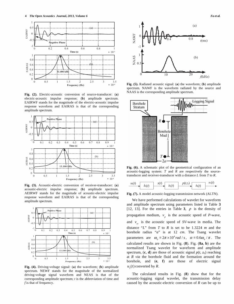
Fig. (5). Radiated acoustic signal: (a) the waveform; (b) amplitude
spectrum. NAWF is the waveform radiated by the source and NAAS is the corresponding amplitude spectrum.
Fig. (6). A schematic plot of the geometrical configuration of an
acoustic-logging system: T and R are respectively the source-transducer and receiver-transducer with a distance L from T to R.
Fig. (7). A model acoustic-logging transmission network (ALTN).
We have performed calculations of wavelet for waveform
and amplitude spectrum using parameters listed in Table 3
[12, 13]. For the entries in Table 3, is the density of
propagation medium, v
p is the acoustic speed of P-wave,
and v
sv is the acoustic speed of SV-wave in media.
The
distance “L” from T to R is set to be 1.3224 m and the
borehole radius “a” is at 12 cm. The Tsang wavelet
parameters are 0
= 2 104 rad / s ,
= 0.60
/ . The
calculated results are shown in Fig. (8). Fig. (8a, b) are the
normalized Tsang wavelet for waveform and amplitude
spectrum, (c, d) are those of acoustic signal p(t, z0) reaching
at R via the borehole fluid and the formation around the
borehole, and (e, f) are those of electric signal
u
3(t) converted by R.
The calculated results in Fig. (8) show that for the
acoustic-logging signal wavelet, the transmission delay
caused by the acoustic-electric conversion of R can be up to
���
�
�
���
�� ��� ��� ��� ��� �
�� �
���
�
���
���
���
�� ��� � ��� � ��� ��
�� ��
�����
�����������
������
������ ��
�����������
���
������� ��
�����
�����������
������
������
�!����� ��
��
���
�
�
���
�� ��� ��� ��� ��� �
�� �
��� �� ��� ��� ���
���
�
���
���
���
�� ��� � ��� � ��� ��
�� ��
�"�������������
�����
�����������
�����
������
�
�!����� ��
��
���
�
�
���
�� ��� ��� ��� ��� �
�� �
��� �� ��� ��� ���
���
�
���
���
���
�� ��� � ��� � ��� ��
�� ��
�"�������������
��
���
������
������������
�
�
�
���
� �� ��
����
����
���� ���� ������� ��� ����� ����� ����

Progress of Application Research on Acoustics The Open Acoustics Journal, 2013, Volume 6 5
3.1886 μs. Compared to the negative head wave amplitude
value of p(t, z) in Fig (8c), the head wave amplitude of u3(t)
in Fig. (8e) has initially a relative decline and then changes
to a positive value. It shows that if the effect of acoustic-
electric conversion of R on the logging signal is neglected,
the measured value of the speed will produce a much larger
error.
Table 3. Physical Parameters of the Borehole Fluid and MC-
Sandstone Around Borehole
Medium
kg m3( )
v
pm s( )
v
s (m/s)
Borehole fluid 1.2 1540
Formation 2.16 5943 3200
Fig. (8). Acoustic-electric conversion of receiver-transducer on the
measured logging signal: (a, b). the normalized Tsang wavelet
spectrum for waveform and amplitude; (c, d). those of acoustic
signal p(t, z0) reaching at R via the borehole fluid and the formation
around the borehole; (e, f). those of electric signal u
3(t) converted
by R.
In traditional cement bond quality logging, if the head-
wave amplitude of acoustic-logging signal is small, the
cement bond quality of the cased-well is defined as good;
otherwise, the cement bond quality is considered as poor.
Now, if the impact of acoustic-electric conversion of R on
the head-wave amplitude is not properly considered, the bad
cementation quality may be misjudged as a good
cementation quality and vice versa [14].
2.3. Addition and Multiplication ALTNs
For an array acoustic-source (AAS) in the borehole at the
radiation directivity maximum, the excitation time delay t
for two neighbor transmitting elements, i.e. the transducers
in ALTN model, is given by [15, 16]
t = d / v , (4)
where, d is the interval between two neighboring
transmitting elements and v is the acoustic velocity of P-
wave in the formation around the borehole. Numerical
analysis has shown that an array acoustic-source ALTN
model with a single receiver is reciprocal to that of a single
source with an array acoustic-receiver (AAR).
Eq. (4) may be used to adjust the excitation time delay of
an array acoustic-source ALTN model with a single receiver.
It is easy see that the head-wave amplitude of acoustic-
logging signal linearly increases with respect to the number
of transducer elements in the AAS. Similarly, to adjust the
shifting time of acoustic-logging signals received by each
receiving elements in ALTN with a single source-transducer,
the head-wave amplitude of acoustic-logging signal
increases also roughly linearly with respect to the number of
transducer elements in the AAR. So, the above mentioned
two ALTNs abide approximately by an addition rule and are
identified as the addition ALTN.
Assume that we have an ALTN network model with N
transducers in AAS and M transducers in AAR. For the
ALTN with AAS and AAR, P-wave velocity around the
borehole is used to adjust the AAS excitation time delay.
The acoustic signals emitted by all transmitting elements in
AAS propagate around the borehole with the same phase.
Then, the propagating signals reach the receiving elements in
AAR and change into electric signals due to the acoustic-
electric conversion of the transducers. Finally, the shifting
time of these electric signals converted by each receiving
elements may be adjusted by solving Eq. (4). The value of
the stacked head-wave amplitude increases approximately as
a product of M and N. In this case, the ALTN model is
identified as a multiplication ALTN.
Now, let’s consider a simple example with N = 4 and M =
4, i.e. AAS and AAR consist of four transducers each. The
interval between two neighboring transducers is set to be 82
mm and the distance from AAS to AAR is taken as 2.44 m.
The calculated acoustic beam directivities for this ALTN are
presented in Fig. (9). Clearly, the acoustic-beam steering
efficiency of the multiplication ALTN is much higher than
that of the addition ALTN. In either case, two equivalent
ALTNs, either addition or multiplication, would increase
greatly the head wave amplitude for the acoustic-logging
signal.
�
���
�
����
��� ��� ��� �� �� � ��� ��� �� �� �
�����
��� � � �/��� �
�� ���
���
���0
��0
��
�
���
��
��0
� ���� ��
���0
��
�
�� �
����0
� ��
� ��
��0
��
�
�� �
�
�
�
���
�
����
��� ��� ��� �� �� � ��� ��� �� �� �
����
�
���
�
����
��� ��� ��� �� �� � ��� ��� �� �� �
����
�
���
� ��� � ��� � ���
����
�
�
���
�� ��� � ��� � ���
����
���
� ��� ��� �� �� � ��� ��� �� �� ��
�
����
�
�
�
�
�
� ���
� ����
� ���
� ����
� ���
� ����
��
�1�
�.�
�)�
�2�
� � �/��� �
������ �
�����
�����������
�������� �
����������
������

6 The Open Acoustics Journal, 2013, Volume 6 Fa et al.
Fig. (9). Acoustic-beam steering directivities of addition and
multiplication ALTNs: curve (1) is the directivities of the two addition ALTNs and curve (2) is that of the multiplication ALTN.
2.4. Acoustic Signal Propagation in Drill-Collar
Acoustic logging while drilling is mainly used for the
acoustic velocity measurement around horizontal wells,
deviated wells on land, and cluster wells on offshore.
Conventional logging method can be applied to acoustic-
logging tool while drilling. Acoustic probes may be used as
either the general acoustic-transducers or multiple acoustic-
transducers. The acquired logging data could be processed
by a proper software program which is written on the electric
circuit module in the acoustic logging tool while drilling
(ALTWD).
The drill-collar is usually made of steel and the outer-
shell of ALTWD is a steel-grooves casing. The ALTWD is
placed in drill collar and the outer-shell of ALTWD is
scheduled for torsion force created during drilling. Bearing
huge torsion force, the drill collar cannot be grooved, or else
it will be ruined. As shown in Fig. (10), there are small
windows on the drill-collar and on the outer-shell of
ALTWD. These windows are located in the vicinity of
source transducers and receiver transducers. The acoustic
signal radiated by the source-transducer in ALTWD can pass
through the pipe layers via the windows, and then reach the
formation around the borehole. The acoustic-signal coming
from the formation can be collected by receiver-transducers
in ALTWD.
One of the technical difficulties with ALTWD is that the
propagation speed of P-wave in steel is typically about 5900
m/s. This speed is usually larger than that of low- or
intermediate-velocity formation in ALTWD. The
propagation path of acoustic signal in drill-collar is actually
shorter than that of formation in ALTWD. Without a specific
design, the acoustic signal from the drill-collar may reach
receiver-transducer unwittingly ahead of the signal from the
formation around the borehole.
To make a specific design, we note that scattering takes
place when acoustic-signal impinges on an interface between
two different media. Applying acoustic-scattering theory and
adopting medium acoustic-absorption technology, the outer-
shell of drill-collar may be properly designed with some
required specifications. By doing so, the outer-shell ensures
that acoustic signal emitted by the source-transducer would
pass fully through the windows on outer-shell of ALTWD,
as well as on drill collars. Due to the acoustic-scattering and
acoustic-absorption the drill-collar inner-wall ensures
that the acoustic signal reaching the drill-collar is scattered
and attenuated. This will ensure the acoustic logging signals
come from the formation around the borehole, rather than
from drill-collar.
Fig. (10). A schematic plot of propagation paths of acoustic signal.
2.5. Reflection/Refraction Between Two Anisotropy Rock Slabs
Amplitude variations with offset (AVO) is one of the
most important analyses in studies of reflection coefficient.
P-wave amplitude variation with respect to an incidence
angle is affected by acoustic impedances of P- and SV-waves
on both sides of the reflector. Ostrander [17] showed that
AVO anomalies can indicate areas of Poisson’s ratio change
and are direct hydrocarbon indicators. However, anisotropy
has potentially significant effects on AVO application and
time-depth conversion of seismic data [18, 19]. It is well
known that elastic anisotropy is so common in Earth’s
interior that it is virtually impossible to avoid it in
geophysical studies. Meanwhile, rock anisotropy is generally
described as transversely isotropic and the presence of this
kind of rock anisotropy can severely distort the AVO
analysis.
In a boundary between two transversely isotropic media
with a vertical axis of symmetry (VTI), two 4th order
polynomials have been established for calculations of
reflection/refraction angles [18],
B
1
(1) sin4 (1,3)+ B
3
(1) sin2 (1,3)+ B
5
(1)= 0, (5)
B
1
(2) sin4 (2,4)+ B
3
(2) sin2 (2,4)+ B
5
(2)= 0. (6)
������
��
�
�
�
�����
���
���
���
���
���
���
���
���
��� ���
�)1)#3)( +(�$�.,1)(4,+)( �*)&&%!2&!""#$"%+!!& 5(#&&%1!&&�(
�!(��+#!$%�(!,$.+*)%!()*!&)
'!()*!&)2&,#.
�!,(1) +(�$�.,1)(

Progress of Application Research on Acoustics The Open Acoustics Journal, 2013, Volume 6 7
In case of a P-wave impinging on the boundary between
two VTI media, the relationship between displacement and
traction across boundary in terms of the reflection/refraction
coefficients can be written as
AR = B , (7)
where, A is a 4 by 4 matrix, and R and B are the 4-element
vectors. The matrix elements of A are given by a
11= u
x
(1),
a
12= u
x
(2),
a
13= u
z
(3), a
14= u
z
( 4 ),
a
21= u
z
(1),
a
22= u
z
(2),
a
23= u
x
(3),
a24
= ux
( 4 ),
a31
=c
13
( in)ux
(1) sin (1)+ c
33
(1)uz
(1) cos (1)
v(1) ( (1) ),
a32
=c
13
(re)ux
(2) sin (2)+ C
33
(re)uz
(2) cos (2)
v(2) ( (2) ),
a33
=c
13
( in)uz
(3) sin (3)+ C
33
( in)ux
(3) cos (3)
v(3) ( (3) ),
a34
= -c
33
(re)ux
(4)sin (4) + c13
(re)uz
(4)cos (4)
v(4)(q(4) ),
a41
=c
44
( in) (ux
(1) cos (1)+ u
z
(1) sin (1) )
v(1) ( (1) ),
a42
=c
44
(re) (ux
(2) cos2
+ uz
(2) sin2)
v(2) ( (2) ),
a43
=c
44
( in) (ux
(3) sin (3)+ u
z
(3) cos (3) )
v(3) ( (3) ),
a44
=c
44
(re) (uz
(4)cos (4)+ u
x
(4)sin (4) )
v (4) ( (4) ).
The elements of B vector are given as b
1= u
x
(1),
b2
= uz
(1),
b3
=c
13
( in)ux
(1) sin (1)+ c
33
( in)uz
(1) cos (1)
v(1) (1)
, and
b4
=c
44
( in) (ux
(1) cos (1)+ u
z
(1) sin (1) )
v(1) ( (1) ). In all these equations
mentioned above, the superscripts {m}={0, 1, 2, 3, 4} denote
incident P-wave or SV-wave (m=0), the reflected P-wave
(m=1), refracted P-wave (m=2), reflected SV-wave (m=3),
and refracted SV-wave (m=4); {n}={in, re} denote the
incidence medium and refraction medium. For the elements
in R vector, R(1)
is the reflection coefficient of quasi-P to
quasi-P wave reflection, R(2)
is the refraction coefficient of
quasi-P to quasi-P wave refraction, R(3)
is the reflection
coefficient of quasi-P to quasi-SV wave reflection and R(4)
is the refraction coefficient of quasi-P to quasi-SV wave
refraction. ux
(m) and u
z
(m) are the polarization coefficients of
the incident and mode conversion waves, and v(m)
is the
phase velocity for the above waves. cij
(n) is the elastic
stiffness of incidence and refraction media.
We have performed calculations of the
reflection/refraction coefficients based on Eqs. (5)-(7), using
the anisotropic parameters of two sedimentary rocks listed in
Table 4. The calculated results are plotted in Fig. (11) and
are readily used for AVO analysis of seismic exploration
data [20].
Table 4. Anisotropic and Physical Parameters of Rocks,
where, and are Vertical Velocity of P-Wave
and SV-Wave in VTI Medium, Respectively; , *
and are the Anisotropic Parameters of VTI
Medium. A-Shale Stands for Anisotropic Shale and
T-Sandstone Stands for Taylor Sandstone
Ansotropy Parameters
Medium
(m/s) (m/s) (g / cm
3 )
*
A-shale 2745 1508 2.340 0.103 -0.073 0.345
T-sandstone 3368 1829 2.500 0.110 -0.127 0.255
2.6. Technology to Inverse Oil Reservoir by Logging and Seismic Data
For various possible geological structures, e.g. thin-out,
top-lap, down-lap, etc. a seismic wavelet dictionary can be
established using logging data from several oil wells in a
given region. A match pursuit can be performed for words in
the dictionary with the seismic exploration data obtained
from this region [21, 22]. Then, the reflectivity series of
underground formation can be obtained from the measured
seismic wavelets and from the words in the seismic wavelet
dictionary. By observing the amplitudes and phases of the
obtained reflectivity series, an oil reservoir may be revealed.
In summary, this technology may be classified as two
parts: creation of the seismic wavelet dictionary and software
processing of reflectivity series inversion.
From the seismic wavelet dictionary, the words presented
in Fig. (12) show a geological structure of a thin-out. Those
in Fig. (13) present a geological structure of an inter-bed,
and those in Fig. (14) reflect a geological structure with two
down-laps.
In calculations of the formation reflectivity series, a
software program is used to scan all words in the seismic-
logging dictionary with every actual measured seismic signal
wavelet. This scan would locate the maximum correlation
coefficient. According to the shift invariance norm, the
iterative calculations are performed by utilizing a match
pursuit algorithm. When the calculation is converged, a
minimal residual between the “words” with a maximal
correlation coefficient is obtained. Then, the trace of actual
seismic signal wavelet is reached to locate the desired oil-gas
reservoirs.

8 The Open Acoustics Journal, 2013, Volume 6 Fa et al.
Fig. (11). Reflection/refraction coefficients versus and (re) when (in) , *(in) and *(re) are fixed. In the figures, (1) , (2) , (3) and (4) are
the phase of R(1) , R(2) , R(3) and R(4) , respectively.
�
��
��
��
��
�������
��������
������
���� ���
����
��
���
��
���
�
������
��������
����
�������
���
����
�����
���
��
��
��
��
������
��������
����
�������
���
����
�����
������
��������
����
�������
���
����
�����
��
�
��
�
���
��
���
�
������
��������
����
�������
���
����
�����
���
���
���
���
������
��������
�������
���� ���
����
�����
���
��
���
�����
����
�������
����
��
��
���
����� ���
���
�����
��������
����
�������
�
����
���
����
�
���
���
���
���
���
���
���
���
��
��
��
��
��
�
�
�
�
�
�
�
� �� ��
��
�� ��
��
�� ��
� �
� �
��
��
��
��
��
'"(�)�� ��������*�
��������*�
��������*�
��������*�
'"(�)��
'"(�)��
'"(�)��

Progress of Application Research on Acoustics The Open Acoustics Journal, 2013, Volume 6 9
Fig. (12). A geological structure of a thin-out.
Fig. (13). A geological structure of an inter-bed.
3. CONCLUDING REMARKS
So far, we have discussed an improved ALTN network
model for acoustical application to petroleum logging and
seismic exploration. It is important to note that in studies of
this new model, we identified intrinsic relationships amongst
various physical quantities, such as driving-voltage signal,
electric-acoustic conversion of source-transducer, acoustic-
electric conversion of receiver-transducer, measured logging
signal, and the propagation media.
Amongst the most important physical concepts proposed
in this paper are acoustic-electric analogue and a driving-
voltage convolution with electric-acoustic impulse response.
The latter concept led to a practical and improved petroleum
logging ALTN in which the convolution of the driving-
voltage signal with the electric-acoustic impulse response
function was used to substitute for some assumed acoustic-
source functions. These assumed functions are usually used
in traditional acoustic-logging models, e.g. Tsang wavelet,
Ricker wavelet, Gaussian impulse wavelet, etc.
Fig. (14). A geological structure with two down-laps.
The anisotropic effects on reflection/refraction between
two different rock-slabs are discussed. Correspondingly, a
new fast algorithm for calculation of reflection/refraction
coefficients has been presented. It provides insight into
analysis of amplitude variations with offset (AVO) for exploring new oil reservoirs or gas fields accurately.
Getting into the prediction of new oil reservoirs and/or
gas fields, the new algorithm leads to the construction of a
seismic wavelet-dictionary which can be constructed by
logging data from several oil wells in a given region. The
reflectivity series of the formation can be obtained accurately
by using the match-pursuit algorithm, the seismic wavelet
dictionary and the measured seismic reflection data.
Within the framework of the newly proposed network
model, there are several other important issues discussed
besides the discussions above, including (i) the notation of
addition and multiplication of acoustic-logging ALTN
transmission network, (ii) the technology of eliminating
acoustic signal propagation in the drill-collar for acoustic-
logging while drilling, and (iii) the effect of rock anisotropy
on reflection/refraction coefficients and its relation to an
accurate AVO analysis.
In summary, the newly proposed ALTN network model
describes the acoustic-logging process based strictly on a
physical mechanism. It is more practical and much closer to
the actual situation of acoustic logging than any earlier
acoustic-logging models. Applications of the new network
model in analysis of acoustic-logging process lead to
accurate acoustic-logging information, such as propagation
velocity, signal amplitude, wavelet phase, and frequency
spectrum of acoustic-logging signal in the formation.
CONFLICT OF INTEREST
The authors confirm that this article content has no conflicts
of interest.
6(�1)%$,�)(
6*#$ !,+
�)#��#1%7�3)&)+�%�!(%7!(.��
6*)%2!,(+*%&�8)(
6*)%�#0+*%&�8)(
6#�)%���
�
���
�
���
�
���
� �� �� � �� �� ��
6#�)%���
6(�1)%$,�)(
�)#��#1%7�3)&)+�%�!(%7!(.��
�$+)(). 6*)%+*#(.%&�8)(
�
���
�
���
�
���
� �� �� � �� �� ��
6#�)%���
6(�1)%$,�)(
�)#��#1%7�3)&)+�%�!(%7!(.���
���
�
���
�
���
� �� �� � �� �� ��
��
5!7$ &�9%�
5!7$ &�9%�
6*)%2#(�+%&�8)(
6*)%+*#(.%&�8)(
6*)%2#2+*%&�8)(
6*)%�)3)$+*%&�8)(

10 The Open Acoustics Journal, 2013, Volume 6 Fa et al.
ACKNOWLEDGEMENTS
This work is supported in part by a grant (No. 40974078)
from the National Natural Science Foundation of China and
by the Physical Sciences Division at The University of
Chicago.
REFERENCES
[1] Larose E, Rosny J, Margerin L, et al. Observation of multiple scattering of kHz vibrations in a concrete structure and application
to monitoring weak changes. Physical Rev E Stat Nonlin Soft Matter Phys 2006; 73(1): 016609.
[2] Tsang L, Rader D. Numerical evaluation of the transient acoustic waveform due to a point source in a fluid-filled bore hole.
Geophysics 1979; 44: 1706-20. [3] Gibson Jr RL, Peng C. Low- and high-frequency radiation from
seismic sources in cased boreholes. Geophysics 1994; 59: 1780-5. [4] Cheng CH, Toksöz MN. Elastic wave propagation in a fluidfilled
borehole and synthetic acoustic logs. Geophysics 1981; 46: 1042-53.
[5] Cerveny V. Seismic ray theory. Cambridge: Cambridge University Press 2001.
[6] Thomsen L. Weak elastic anisotropy. Geophysics 1986; 51: 1954-66.
[7] Wang Y. Seismic time-frequency spectral decomposition by matching pursuit. Geophysics 2007; 72: 13-20.
[8] Fa L, Castagna JP, Hovem JM. Derivation and simulation of source function for acoustic-logging. IEEE Ultrasonics Symposium
Proceedings; 1999 November; Lake Tahoe, USA 1999. [9] Fa L, Castagna JP, Hovem JM, Dong DQ. An acoustic-logging
transmission-network model. J Acoust Soc Am 2002; 111: 2158-65.
[10] Fa L, Castagna JP, Suarez-Rivera R, Sun P. An acoustic-logging
transmission-network model (continued): Addition and multiplication ALTNs. J Acoust Soc Am 2003; 113: 2698-703.
[11] The Product Catalogue of CHANNEL Industries, Inc., 839 Ward Drive, Santa Barbara, CA 93111, USA 1992
[12] Gong W. Full waveform analysis of acoustic well logging and its multidimimensional procession methods. Ph.D. thesis. China:
Southeast University, July 1988. [13] Fa L, Castagna JP, Hovem JM, Dong D. An acoustic-logging
transmission-network model. J Acoust Soc Am 2002; 111: 2158-65.
[14] Fa L, Xie WY, Tian Y, Zhao MS, MA L, DONG DQ. Effects of electric-acoustic and acoustic-electric conversions of transducers
on acoustic-logging signal. Chin Sci Bull 2012; 57: 1246-60. [15] Fa L. Application of phase control array technique to sonic logging.
Proceedings of The China-Japan Joint Conference on Ultrasonics; 1987 April, Nanjing: China 1987.
[16] Fa L, Ma HF. Design of a new type of array transmitting sonic logging. Acta Petrolei Sin 1991; 12: 52-7.
[17] Ostrander WJ. Plane wave reflection coefficients for gas sands at nonnormal angles of incidence. Geophysics 1984; 49: 1637-48.
[18] Fa L, Brown RL, Castagna JP. Anomalous post-critical refraction behavior for certain transversely isotropic media. J Acoust Soc Am
2006; 120: 3479-92. [19] Zhao Y, Zhao N, Fa L, Zhao M. Seismic signal and data analysis of
rock media with vertical anisotropy. J Mod Phys 2013; 4: 11-8. [20] Castagna JP. Offset-dependent reflectivity: theory and practice of
AVO analysis. Oklahama, Tuba, USA: Society of Exploration Geophysicists 1993.
[21] Mallat S, Zhang Z. Matching pursuit with time-frequency dictionaries. IEEE Trans Signal Proc 1993; 44(12): 3397-415.
[22] Davis G, Mallat S, Avellaneda M. Adaptive greedy approximat-ions. Constr Approximation 1997; 13: 57-98.
Received: November 15, 2012 Revised: January 16, 2013 Accepted: January 23, 2013
© Fa et al.; Licensee Bentham Open.
This is an open access article licensed under the terms of the Creative Commons Attribution Non-Commercial License (http://creativecommons.org/licenses/by-nc/3.0/)
which permits unrestricted, non-commercial use, distribution and reproduction in any medium, provided the work is properly cited.