
Research Article Pricing Convertible Bonds with Credit...
14
Research Article Pricing Convertible Bonds with Credit Risk under Regime Switching and Numerical Solutions Wei-Guo Zhang and Ping-Kang Liao School of Business Administration, South China University of Technology, Guangzhou 510640, China Correspondence should be addressed to Wei-Guo Zhang; [email protected] Received 26 December 2013; Accepted 9 April 2014; Published 19 May 2014 Academic Editor: Fenghua Wen Copyright © 2014 W.-G. Zhang and P.-K. Liao. is is an open access article distributed under the Creative Commons Attribution License, which permits unrestricted use, distribution, and reproduction in any medium, provided the original work is properly cited. is paper discusses the convertible bonds pricing problem with regime switching and credit risk in the convertible bond market. We derive a Black-Scholes-type partial differential equation of convertible bonds and propose a convertible bond pricing model with boundary conditions. We explore the impact of dilution effect and debt leverage on the value of the convertible bond and also give an adjustment method. Furthermore, we present two numerical solutions for the convertible bond pricing model and prove their consistency. Finally, the pricing results by comparing the finite difference method with the trinomial tree show that the strength of the effect of regime switching on the convertible bond depends on the generator matrix or the regime switching strength. 1. Introduction Convertible bond is a kind of the most important financing instruments, so the convertible bond market occupies an important position in the international financial market. American convertible bond market is the largest market in the world, and it has issued more than 400 trillion dollars in total from 1980 to 2011. Hong Kong is an international financial center; there are about 70 trillion yuan of convertible bonds in 2012. Although the amount of convertible bonds issued in developing countries is much less than that in developed countries, the convertible bonds markets of some countries are developing rapidly. For example, China issued more than 60 trillion yuan of new convertible bonds in 2010, which is almost three times the level of four years ago. Because of the importance of the convertible bonds in the financial market, the convertible bond pricing problem is a hot topic. Taking the corporate value as a basic variable, Ingersoll [1] constructed a structural model for pricing convertible bonds by deriving a Black-Scholes-type partial differential equation based on Black-Scholes’ theory. Following the work of Inger- soll [1], Brennan and Schwartz [2] explored the valuation of the convertible bonds with dividends and callable provision. However, the structural approach has a shortcoming which is the fact that the data of the corporate value is difficult to measure and observe. To overcome this shortcoming, McConnell and Schwartz [3] firstly selected the stock price as the basic variable, which becomes a mainstream later. With further research, the clauses of convertible bond also are in- depth studied. Kimura and Shinohara [4] and Yang et al. [5] explored the effect of reset clause on noncallable convertible bonds; they also derived an exact solution on the valuation of the convertible bonds with and without dilution effect. e numerical solutions are also adapted to price the convertible bonds. Brennan and Schwartz [6] took stochastic interest rate into account firstly and built the so-called two-factor model for convertible bond pricing that is popular since it is available. en, a three-factor model was established by Davis and Lischka [7] to value the convertible bonds with stochastic credit risk. To solve the complex multifactor models, characteristics/finite elements and trinomial tree model are applied to the valuation of the convertible bonds such as Barone-Adesi et al. [8] and Xu [9]. Some other researches consider special convertible bonds or other factors of the convertible bonds. Yagi and Sawaki [10] proposed a valuation model of callable-puttable reverse convertible bonds, which are issued by a company to be exchanged for the shares of another company. Instead of the popular geometric Hindawi Publishing Corporation Mathematical Problems in Engineering Volume 2014, Article ID 381943, 13 pages http://dx.doi.org/10.1155/2014/381943
Transcript of Research Article Pricing Convertible Bonds with Credit...
Research ArticlePricing Convertible Bonds with Credit Risk under RegimeSwitching and Numerical Solutions
Wei-Guo Zhang and Ping-Kang Liao
School of Business Administration South China University of Technology Guangzhou 510640 China
Correspondence should be addressed to Wei-Guo Zhang wgzhangscuteducn
Received 26 December 2013 Accepted 9 April 2014 Published 19 May 2014
Academic Editor Fenghua Wen
Copyright copy 2014 W-G Zhang and P-K Liao This is an open access article distributed under the Creative Commons AttributionLicense which permits unrestricted use distribution and reproduction in any medium provided the original work is properlycited
This paper discusses the convertible bonds pricing problem with regime switching and credit risk in the convertible bond marketWe derive a Black-Scholes-type partial differential equation of convertible bonds and propose a convertible bond pricing modelwith boundary conditions We explore the impact of dilution effect and debt leverage on the value of the convertible bond andalso give an adjustment method Furthermore we present two numerical solutions for the convertible bond pricing model andprove their consistency Finally the pricing results by comparing the finite difference method with the trinomial tree show thatthe strength of the effect of regime switching on the convertible bond depends on the generator matrix or the regime switchingstrength
1 Introduction
Convertible bond is a kind of the most important financinginstruments so the convertible bond market occupies animportant position in the international financial marketAmerican convertible bond market is the largest market inthe world and it has issued more than 400 trillion dollarsin total from 1980 to 2011 Hong Kong is an internationalfinancial center there are about 70 trillion yuan of convertiblebonds in 2012 Although the amount of convertible bondsissued in developing countries is much less than that indeveloped countries the convertible bonds markets of somecountries are developing rapidly For example China issuedmore than 60 trillion yuan of new convertible bonds in 2010which is almost three times the level of four years ago Becauseof the importance of the convertible bonds in the financialmarket the convertible bond pricing problem is a hot topic
Taking the corporate value as a basic variable Ingersoll [1]constructed a structural model for pricing convertible bondsby deriving a Black-Scholes-type partial differential equationbased on Black-Scholesrsquo theory Following the work of Inger-soll [1] Brennan and Schwartz [2] explored the valuation ofthe convertible bonds with dividends and callable provisionHowever the structural approach has a shortcoming which
is the fact that the data of the corporate value is difficultto measure and observe To overcome this shortcomingMcConnell and Schwartz [3] firstly selected the stock price asthe basic variable which becomes a mainstream later Withfurther research the clauses of convertible bond also are in-depth studied Kimura and Shinohara [4] and Yang et al [5]explored the effect of reset clause on noncallable convertiblebonds they also derived an exact solution on the valuation ofthe convertible bonds with and without dilution effect Thenumerical solutions are also adapted to price the convertiblebonds Brennan and Schwartz [6] took stochastic interestrate into account firstly and built the so-called two-factormodel for convertible bond pricing that is popular sinceit is available Then a three-factor model was establishedby Davis and Lischka [7] to value the convertible bondswith stochastic credit risk To solve the complex multifactormodels characteristicsfinite elements and trinomial treemodel are applied to the valuation of the convertible bondssuch as Barone-Adesi et al [8] and Xu [9] Some otherresearches consider special convertible bonds or other factorsof the convertible bonds Yagi and Sawaki [10] proposeda valuation model of callable-puttable reverse convertiblebonds which are issued by a company to be exchanged for theshares of another company Instead of the popular geometric
Hindawi Publishing CorporationMathematical Problems in EngineeringVolume 2014 Article ID 381943 13 pageshttpdxdoiorg1011552014381943
2 Mathematical Problems in Engineering
Brownian motion model Labuschagne and Offwood [11]valued the convertible bonds with the CGMY stock priceprocess Lee and Yang [12] presented the unexplained portionof the valuationmodel of convertible bonds based onMCDM
Credit risk is another important factor that affects thevalue of convertible bonds As early as the structural approachis available the credit risk is considered by comparing thecorporate value and the convertible bond value Howeverthis idea is not popular for the shortcoming of the structuralapproach There are two main ways to deal with the creditrisk in the pricing models now One way measures the creditrisk by the credit spread of bonds McConnell and Schwartz[3] applied this idea to the valuation of the convertible bondsTsiveriotis and Fernandes [13] innovatively defined the ldquocashonly part of the convertible bondsrdquo whose discount ratecontains credit spread and is different from the rest of theconvertible bonds This idea is also applied in binomial treetrinomial tree andmultifactormodel of the convertible bondpricing with credit risk such as the work of Bardhan et al[14] The other way measures the credit risk by the defaultintensityThedefault intensity to price convertible bondswithcredit risk was introduced to measure the credit risk in theearly work of Duffie and Singleton [15] and Takahashi et al[16] However these works are not reasonable enough forthey cannot measure the credit risk accurately so that theyneed to be improvedThus Ayache et al [17] proposed a newmodel for the convertible bonds pricingwith credit risk (AFVmodel) Different from previous work they adopt defaultintensity to measure the credit risk and build a model byderiving the PDE of the convertible bonds This idea is alsointroduced to trinomial tree and multifactor model such asthe work of Chambers and Liu [18] Milanov et al [19] seta binomial tree model for the valuation of convertible bondand prove that their model converges in continuous time tothe AFV model
Since the early 20th century the global economy inter-changes between the boom and the bust frequently Similarlythe security market also interchanges between the ldquobullmarketrdquo and the ldquobear marketrdquo frequently The stock priceprocesses have different characteristics in different states ofeconomy Considering the regime switching some optionspricing models with regime switching are proposed Theoptions pricing with regime switching can be traced back tothe work of Naik [20] who establishes a formula of optionpricing with only two states Then Buffington and Elliot[21] built pricing models of European options and Americanoptions with regime switching that the number of states isuncertain but finite The valuation of exotic options was alsostudied by Boyle and Draviam [22] with finite differencemethod Yuen and Yang [23] proposed a modified trinomialtree model to price complex options with regime switch-ing The valuation of the currency options with stochasticvolatility and stochastic interest rate under regime switchingwas studied by Siu et al [24] later Goutte [25] consideredgeneral regime switching stochastic volatility models whereboth the asset and the volatility dynamics depend on thevalues of a Markov jump process and obtain pricing andhedging formulae by risk minimization approach As a kindof medium-term or long-term securities the value of the
convertible bonds may be affected by the regime switchingThe regime switching is also considered in the convertiblebond pricing Song et al [26] developed a valuation modelfor a perpetual convertible bond by the valuation model forthe perpetual American option However they do not takecredit risk dilution effect and debt leverage into account andthe perpetual convertible is not the most common kind ofconvertible bond
The value of the convertible bond is affected by creditrisk market environment dilution and so forth As we knowthe financial leverage of the corporate has also effect onthe return of shareholders which will affect the convertiblebonds finally This paper will discuss the pricing convertiblebondswith credit risk under regime switching which take thedilution effect and the debt leverage into account The rest ofthis paper is organized as follows Section 2 derives the Black-Scholes-type partial differential equation of the convertiblebonds and proposes the theoretical model Section 3 consid-ers the debt leverage and gives amodification of the historicalvolatility Section 4 introduces main details of the numericalsolutions and proves their consistency Section 5 presents anumerical analysis for the features of the convertible bondsFinally the main conclusions are given in Section 6
2 Theoretical Model of the ConvertibleBond Pricing
In this section we derive the Black-Scholes-type partialdifferential equation of the convertible bonds and try to buildup the pricing model Firstly we give the dynamic processof the stock price 119878 and the process of the bond value 119861Here we assume that the states of the economy are modeledby a continuous-time finite-state observable Markov chain119883 = 119883
119905 119905 ge 0 on a complete probability space (ΩFP)
with a finite-state space 120594 = 1198901 1198902 119890
119871 where unit vector
119890119896= (0 0 1 0 0)
1015840isin R119871 represents the 119896th regime or
the 119896th state Let 119860 = 119886119894119895119894119895=12119871
be the generator matrix ofthe Markov chain 119883 which satisfies the following formula
119871
sum
119895=1
119886119894119895= 0 119894 = 1 2 119871 (1)
Then the semimartingale decomposition of continuous-timeMarkov chain119883 is given by
119889119883119905= 119860119883
119905119889119905 + 119889119872
119905 (2)
where119872 = 119872119905 119905 ge 0 is anR119871-valued martingale
Let 119903 = 119903119905| 119905 ge 0 be the process of risk-free rate In the
market with regime switching the risk-free rate only dependson the current state of the market so the risk-free rate at time119905 can be expressed by inner product form as
119903119905= 119903 (119883
119905) = ⟨r 119883
119905⟩ (3)
where r = (1199031 1199032 119903
119871) isin R119871 Similarly let 120583 = 120583
119905 119905 ge 0
119902 = 119902119905 119905 ge 0 and 120590 = 120590
119905 119905 ge 0 be the appreciation rate
Mathematical Problems in Engineering 3
the continuous dividend rate and the volatility of underlyingstock respectively They can be expressed as
120583119905= 120583 (119883
119905) = ⟨120583 119883
119905⟩ 119902
119905= 119902 (119883
119905) = ⟨q 119883
119905⟩
120590119905= 120590 (119883
119905) = ⟨120590 119883
119905⟩
(4)
Here 120583 = (1205831 1205832 120583
119871) isin R119871 q = (119902
1 1199022 119902
119871) isin R119871
and 120590 = (1205901 1205902 120590
119871) isin R119871
Continuous process 119861 = 119861119905 119905 ge 0 denotes the process
of bond value without risk as
119889119861119905= 119903119905119861119905119889119905 (5)
Following the assumptions at the first of this part the stockprice process with initial value 119878
0satisfies the equation
119889119878119905= (120583119905minus 119902119905) 119878119905119889119905 + 120590
119905119878119905119889119882119905 (6)
where119882 = 119882119905119905isin[0119879]
is a standard Brownian motionWe consider a convertible bond with maturity 119879 and
face value 119865 Without losing generality we assume that theconvertible bond has the following clauses (1)The convert-ible bond pays a fixed coupon amount 119888
119894at time 119905119888
119894(119894 =
1 2 119872) (2) The convertible bond can be converted to120581 share after time 119879con (0 le 119879con le 119879) (3) The convertiblebond is callable by the issuers at an interval price119861
119888after time
119879call (119879con le 119879call le 119879) (4) The convertible bond is puttableby the holders at a price 119861
119901after time 119879put (119879con le 119879put le 119879)
Let119881119896(119896 = 1 2 119871) be the price of convertible bond at the
119896th regime and set V = (1198811 1198812 119881
119871)
We now consider the valuation of the convertible bondswith credit risk under regime switching When the companygoes bankrupt the holders of the convertible bonds can getsome compensation which is usually less than 119865 What ismore if all assets of the company are more valuable thanall debt or the company is merged or reorganized the stockof the company is still valuable Therefore we make thefollowing assumptions
(1) The default probability approximately is equal to 120582119905119889119905
for 119889119905 where 120582119905= 120582(119883
119905) = ⟨120582 119883
119905⟩ and 120582 =
(1205821 1205822 120582
119871)
(2) Upon default the holders can choose to receive thecompensation 119877
119905119865 per convertible bond or convert to
120581(1 minus 120578119905) shares Here 119877
119905= 119877(119883
119905) = ⟨R 119883
119905⟩ is the
recovery factor and 120578119905= 120578(119883
119905) = ⟨120578 119883
119905⟩ is the jump
ratio of underlying stock SetR = (1198771 1198772 119877
119871) and
120578 = (1205781 1205782 120578
119871)
In the following discussion we try to establish thepricingmodel of convertible bonds by constructing a hedgingportfolio based on no arbitrage principle We assume thatthe hedging portfolio prod includes a convertible bond 119881
119905and
minus120573119905shares 119878
119905at time 119905 When there is no coupon payment in
[119905 119905 + 119889119905] the value of hedging portfolio at time 119905 is
prod
119905
= 119881119905minus 120573119905119878119905 (7)
Absent of default the change in value of the hedging portfolioafter time 119889119905 is
119889119881 minus 120573119905119889119878 (8)
Upon default the loss of the hedging portfolio after time 119889119905is(119881119905minus 120573119905119878119905) minus (max 120581 (1 minus 120578
119905) 119878119905 119877119905119861 minus 120573
119905(1 minus 120578
119905) 119878119905)
= 119881119905minus 120573119905120578119905119878119905minusmax 120581 (1 minus 120578
119905) 119878119905 119877119905119861
(9)
As the default probability is 120582119905119889119905 and no default probability
is 1 minus 120582119905119889119905 in time 119889119905 the expected change in value of the
hedging portfolio after time 119889119905 is the weighted average of thehedging portfolio value change upon default and absent ofdefault as119889prod
119905
= (1 minus 120582119905119889119905) (119889119881 minus 120573
119905119889119878)
minus 120582119905119889119905 (119881119905minus 120573119905120578119905119878119905minusmax 120581 (1 minus 120578
119905) 119878119905 119877119905119861)
(10)
Applying Ito formula with regime switching to (10) we have
119889prod
119905
= [120597119881
120597119905+ (120583119905minus 119902119905) 119878119905
120597119881
120597119878+1
21205902
1199051198782
119905
1205972119881
1205971198782minus 120573120583119905119878119905]119889119905
+ 120582119905119889119905 (119881119905minus 120573119905120578119905119878119905) + 120582119905119889119905max 120581 (1 minus 120578
119905) 119878119905 119877119905119861
+ (120583119905119878119905
120597119881
120597119878minus 120573119905120583119905119878119905)119889119882119905+ ⟨V 119889119883
119905⟩
(11)
Following the no arbitrage principle we have
119889prod
119905
= 119903119905prod
119905
119889119905 (12)
That is119903119905(119881119905minus 120573119905119878119905) 119889119905
= [120597119881
120597119905+ (120583119905minus 119902119905) 119878119905
120597119881
120597119878
+1
21205902
1199051198782
119905
1205972119881
1205971198782minus 120573120583119905119878119905+ 120582119905(119881119905minus 120573119905120578119905119878119905)
+120582119905max 120581 (1 minus 120578
119905) 119878119905 119877119905119861 + ⟨V 119860119883
119905⟩ ] 119889119905
+ (120583119905119878119905
120597119881
120597119878minus 120573119905120583119905119878119905)119889119882119905+ ⟨V 119889119872
119905⟩
(13)
Similar to Buffington and Elliot [21] all the terms in the rightof (13) must be equal to the left of equation that is
120583119905119878119905
120597119881
120597119878minus 120573119905120583119905119878119905= 0 or 120597119881
120597119878= 120573119905 (14)
Consider119903119905(119881119905minus 120573119905119878119905) 119889119905
=120597119881
120597119905+ (120583119905minus 119902119905) 119878119905
120597119881
120597119878
+1
21205902
1199051198782
119905
1205972119881
1205971198782minus 120573120583119905119878119905+ 120582119905(119881119905minus 120573119905120578119905119878119905)
+ 120582119905max 120581 (1 minus 120578
119905) 119878119905 119877119905119861 + ⟨V 119860119883
119905⟩
(15)
4 Mathematical Problems in Engineering
Substituting (14) into (15) we obtain
120597119881
120597119905+ (119903119905minus 119902119905+ 120582119905120578119905) 119878119905
120597119881
120597119878
+1
21205902
1199051198782
119905
1205972119881
1205971198782minus (119903119905+ 120582119905) 119881119905+ ⟨V 119860119883⟩
+ 120582119905max 120581 (1 minus 120578
119905) 119878119905 119877119905119861 = 0
(16)
Equation (16) is partial difference equation or the so-calledBlack-Scholes-type partial differential equation of the con-vertible bond price with credit risk under regime switching
119903119896= ⟨r 119890
119896⟩ 119902
119896= ⟨q 119890
119896⟩ 120590
119896= ⟨120590 119890
119896⟩
120582119896= ⟨120582 119890
119896⟩ 120578
119896= ⟨120578 119890
119896⟩ 119877
119896= ⟨R 119890
119896⟩
119881119896= 119881119896119905= ⟨V 119890
119896⟩ 119896 = 1 2 119871
(17)
Equation (16) can be rewritten as
120597119881119896
120597119905+ (119903119896minus 119902119896+ 120582119896120578119896) 119878119905
120597119881119896
120597119878+1
21205902
1198961198782
119905
1205972119881119896
1205971198782minus (119903119896+ 120582119896) 119881119896
+
119873
sum
119897=1
119886119896119897119881119897+ 120582119896max 120581119878
119905(1 minus 120578
119896) 119877119896119861 = 0
119896 = 1 2 119871
(18)
We must notice that (18) is only applicable during twocoupon payments When the coupon payment is paid theprice per convertible bond will be reduced by the amount ofcoupon at once Therefore the price of the convertible bondsat time 119905119888
119894satisfies
119881+
119905119888119894= 119881minus
119905119888119894minus 119888119894 119894 = 1 2 119872 minus 1 (19)
When all investors convert their convertible bonds someliabilities become the ownerrsquos equity and the number of sharesincreases We assume that the company issues 119898 stocks and119899 convertible bonds If all convertible bonds are convertedat time 119905 ownerrsquos equity value is 119898119878
119905+ 119899119865 totally As the
number of stocks becomes 119898 + 119899120581 the value per stock is(119898119878119905+ 119899119865)(119898 + 119899120581) which is less than 119878
119905when 119878
119905gt 119865120581
This is the so-called dilution effect in convertible bonds Sothe investor will get 120581(119898119878
119905+119899119865)(119898+119899120581) rather than 120581119878
119905per
convertible bond when the convertible bonds are convertedThus the dilution effect can be adjusted by changing thepayment of the convertible bonds
A rational investor seeks to maximize the value of theconvertible bond at any timeThe value of a convertible bondmust be greater than or equal to its conversion value duringthe conversion time Thus we get the conversion provision
119881119896119905ge(119898119878119905+ 119899119865) 120581
119898 + 119899120581 119905 isin [119879con 119879] (20)
At last time 119879 the company will give a return which is morethan or equal to face return to call the convertible bondsThus at time 119879 the value of convertible bonds must be
119881119896119879
= max(119898119878119879+ 119899119861) 120581
119898 + 119899120581 119865 + 119888
119872 (21)
Thus we get the terminal condition of the partial differenceequation (18) If the convertible bonds are puttable at time 119905the investor can get at least 119861
119901for par convertible bondThus
we get the put provision as
119881119896119905ge 119861119901 119905 isin [119879put 119879] (22)
Similarly the value of a convertible bondmust be less than themaximum of conversion value and 119861
119888when the convertible
bonds are callable at time 119905 or the convertible bonds will becalled by the company This call provision can be written as
119881119896119905le max
(119898119878119905+ 119899119865) 120581
119898 + 119899120581 119861119888 119905 isin [119879call 119879] (23)
Considering constraints of the convertible bonds includ-ing conversion provision put provision and call provisionwe get the pricingmodel of convertible bonds with credit riskunder regime switching as follows
120597119881119896
120597119905+ (119903119896minus 119902119896+ 120582119896120578119896) 119878119905
120597119881119896
120597119878
+1
21205902
1198961198782
119905
1205972119881119896
1205971198782minus (119903119896+ 120582119896) 119881119896+
119873
sum
119897=1
119886119896119897119881119897
+ 120582119896max 120581119878
119905(1 minus 120578
119896) 119877119896119865 = 0
119881119896119879
= max(119898119878119879+ 119899119861) 120581
119898 + 119899120581 119865 + 119888
119872
119881119896119905ge(119898119878119905+ 119899119865) 120581
119898 + 119899120581 119905 isin [119879con 119879]
119881119896119905ge 119861119901 119905 isin [119879put 119879]
119881119896119905le max
(119898119878119905+ 119899119865) 120581
119898 + 119899120581 119861119888 119905 isin [119879call 119879]
119881+
119896119905119888119894= 119881minus
119896119905119888119894minus 119888119894 119894 = 1 2 119872 minus 1
(24)
In fact the model (24) is a boundary value problem Wecan solve this boundary value problem by using the theoryof partial difference equation But the boundary problem isdifficult that it has no explicit solution What is more if weset 1205821= 1205822= sdot sdot sdot = 120582
119871= 0 the model (24) becomes the
pricing model of the convertible bonds without credit riskHence we can treat the pricing model without credit risk asa special case of the model (24)
3 Dilution Effect and Debt Leverage
As King [27] showed dilution and leverage have effect onthe value of convertible bond Thus the dilution effect and
Mathematical Problems in Engineering 5
debt leverage will be considered in the pricing model in thissection The dilution effect of the convertible bonds stemsfrom the issuance of new shares when the convertible bondsare converted In the model (24) the dilution effect hasbeen taken into account Thus we only consider the debtleverage in the following discussion As we know the debtleverage or financial leverage is often used as an indicator offinancial risk So once the debt leverage changes the risk ofshareholdersrsquo returns may be changed Hence the volatilityof the shares returns will be affected by debt leverage Thisinspires us to modify the volatility to reflect the effect ofthe debt leverage on the convertible bond value Thus thevolatility in the pricing model of the convertible bondsshould be the volatility after the convertible bond issues ormodification of historical volatility before convertible bondissues
MM theory about the impact of the financial leverage onthe capital cost and the risk provides us with a good ideato deal with the debt leverage For simplicity we add somenecessary assumptions based on the Black-Scholes theory asfollows
(1) No convertible bond issuance cost The convertiblebond issues at par value
(2) There are no new bonds the convertible bonds andthe warrants issuing during the existence of theconvertible bonds The level of debt is stable duringthe existence of the convertible bonds
(3) The operational efficiency risk is unchanged duringthe existence of the convertible bonds and the returnand risk of the capital are the same as before
(4) The return rate and volatility of the stocks are the sameas that of the ownership
Following the assumptions and MM theory we havethe modification of the historical volatility of the stocks asProposition 1
Proposition 1 There are 119898 stocks and 119899 convertible bondsissued by the company right now Let 119864 119863
0 and 119863
1be the
market value of the company ownerrsquo equity the market value ofcorporate liabilities and the total face value of the convertiblebonds Let 120590
1198960and 120590
1198961(119896 = 1 2 119871) be the volatility of the
stocks at 119896th regime before and after the convertible bonds issueLet 120588 be income tax rate of enterprise Then
1205901198961
=119864 + (119863
0+ 1198631) (1 minus 120588)
119864 + 1198630(1 minus 120588)
1205901198960
=1198981198780+ (1198630+ 119898119865) (1 minus 120588)
1198981198780+ 1198630(1 minus 120588)
1205901198960
(25)
Proof Let 1199031198960
and 1199031198961
be the returns of ownerrsquos equity atthe 119896th regime Let 119903
119896119906and 120590
119896119906be the corporate returns
and the volatility at the 119896th regime without any debt Let 119903119896119889
be the average rate of the corporate debt at the 119896th regimeBecause there is not any income except the convertiblebonds when the convertible bonds issue the ownerrsquos equityis unchanged Then the relationship between the rate of
shareholders returns with and without debt at the 119896th regimesatisfies
1199031198960
= 119903119896119906
+1198630
119864(119903119896119906
minus 119903119896119889) (1 minus 120588)
=119864 + 119863
0(1 minus 120588)
119864119903119896119906
minus1198630(1 minus 120588)
119864119903119896119889 119896 = 1 2 119871
(26)
Because 119903119896119889
is constant when the debt is known taking thevariance of both sides of (26) we have
1205902
1198960= Var [119903
1198960] = (
119864 + 1198630(1 minus 120588)
119864)
2
Var [119903119896119906]
= (119864 + 119863
0(1 minus 120588)
119864120590119896119906)
2
(27)
Similarly we can derive the relationship between the volatilitybefore and after the convertible bonds issue as follows
1205902
1198961= Var [119903
1198961] = (
119864 + (1198630+ 1198631)(1 minus 120588)
119864120590119896119906)
2
= (119864 + (119863
0+ 1198631) (1 minus 120588)
119864 + 1198630(1 minus 120588)
1205901198960)
2
(28)
Comparing (27) and (28) we deduce
1205901198961
=119864 + 119863
0+ 1198631
119864 + 1198630
1205901198960
=1198981198780+ (1198630+ 119899119865) (1 minus 120588)
1198981198780+ 1198630(1 minus 120588)
1205901198960
(29)
This completes the proof
Following Proposition 1 we can easily get modifiedvolatility of the model (24) when debt leverage is consideredBut it is worth noting that the method is only applicablefor historical volatility not for implied volatility and othervolatilities which are the current volatilities after the convert-ible bonds issue so that the debt leverage is concluded and thevolatilities are not necessary to be modified
4 Numerical Solutions
The pricing model of the convertible bonds with credit riskunder regime switching introduced in Section 2 is complexand hard to achieve an exact solution so we need thenumerical solution method to solve this model The mainnumerical solution methods of convertible bonds pricinginclude the finite difference method the finite elementmethod the binomial or the trinomial tree and the MonteCarlo simulation The finite difference method is a basic onethat solves directly the partial difference equation with theboundary conditionsThe treemodel is another basic one thatsolves the pricing problembased on the process of stock priceWhat is more without regime switching it is known that thetree model is consistent with the finite difference methodHere we will choose the finite difference method and the treemodel to solve the pricing problem In this section we willgive the details of the finite difference and the trinomial treeto solve this pricing model and explore their consistency
6 Mathematical Problems in Engineering
41 The Finite Difference Scheme The finite differencemethod is the most basic numerical solution of convertiblebond pricing by solving the partial difference equation Wecan improve the accuracy and get satisfactory result byincreasing time steps and price steps For convergence effectand convergence rate of the finite differencemethod we applythe Crank-Nicolson method to solve the model (18) and getapproximate solution Divide the area [119905 119879] times [0 119878max] into119872 times 119873 small identical rectangles Set Δ119905 = (119879 minus 119905)119872 andΔ119878 = 119878max119873 Let 119881
119896119894119895be the price of the convertible bond
under the 119896th regime time 119894Δ119905 and stock price119895Δ119905 To get theEuler explicit scheme we write the difference approximationas120597119881119896
120597119905=119881119896119894+1119895
minus 119881119896119894119895
Δ119905
120597119881119896
120597119878=119881119896119894119895+1
minus 119881119896119894119895minus1
2Δ119878
1205971198812
119896
1205972119878=119881119896119894119895+1
+ 119881119896119894119895minus1
minus 2119881119896119894119895
Δ1198782
(30)
Substituting (30) in (18) we have
119881119896119894+1119895
minus 119881119896119894119895
Δ119905+ (119903119896minus 119902119896+ 120582119896120578119896) 119895Δ119878
119881119896119894119895+1
minus 119881119896119894119895minus1
2Δ119878
+1
21205902
1198961198952Δ1198782119881119896119894119895+1
+ 119881119896119894119895minus1
minus 2119881119896119894119895
Δ1198782minus (119903119896+ 120582119896) 119881119896119894119895
+ 120582119896max (119877
119896119861 120581 (1 minus 120578
119896) 119895Δ119878) +
119871
sum
119897=1
119886119896119897119881119897119894119895
= 0
(31)
To get the Euler implicit scheme we write the differenceapproximation as
120597119881119896
120597119905=119881119896119894+1119895
minus 119881119896119894119895
Δ119905
120597119881119896
120597119878=119881119896119894+1119895+1
minus 119881119896119894+1119895minus1
2Δ119878
1205971198812
119896
1205972119878=119881119896119894+1119895+1
+ 119881119896119894+1119895minus1
minus 2119881119896119894+1119895
Δ1198782
(32)
Substituting (32) in (18) we get
119881119896119894+1119895
minus 119881119896119894119895
Δ119905+ (119903119896minus 119902119896+ 120582119896120578119896) 119895Δ119878
119881119896119894+1119895+1
minus 119881119896119894+1119895minus1
2Δ119878
+1
21205902
1198961198952Δ1198782119881119896119894+1119895+1
+ 119881119896119894+1119895minus1
minus 2119881119896119894+1119895
Δ1198782
minus (119903119896+ 120582119896) 119881119896119894119895
+ 120582119896max (119877
119896119861 120581 (1 minus 120578
119896) 119895Δ119878)
+
119871
sum
119897=1
119886119896119897119881119897119894119895
= 0
(33)
By (31) and (33) we obtain
119881119896119894+1119895
minus 119881119896119894119895
Δ119905+ (119903119896minus 119902119896+ 120582119896120578119896)
times 119895119881119896119894119895+1
minus 119881119896119894119895minus1
+ 119881119896119894+1119895+1
minus 119881119896119894+1119895minus1
4
minus (119903119896+ 120582119896) 119881119896119894119895
+
119871
sum
119897=1
119886119896119897119881119897119894119895
+1
41205902
1198961198952(119881119896119894+1119895+1
+ 119881119896119894+1119895minus1
minus 2119881119896119894+1119895
+119881119896119894119895+1
+ 119881119896119894119895minus1
minus 2119881119896119894119895
)
+ 120582119896max (119877
119896119861 120581 (1 minus 120578
119896) 119895Δ119878) = 0
(34)
Multiplying Δ119905 at both sides of (34) transposing and simpli-fying we get
[1
4(119903119896minus 119902119896+ 120582119896120578119896) 119895Δ119905 minus
1
41205902
1198961198952Δ119905]119881119896119894119895minus1
+ [1 +1
4(119903119896+ 120582119896) 119895Δ119905 +
1
21205902
1198961198952Δ119905]119881119896119894119895
+ [minus1
4(119903119896minus 119902119896+ 120582119896120578119896) 119895Δ119905 minus
1
41205902
1198961198952Δ119905]119881119896119894119895+1
minus
119871
sum
119897=1
119886119896119897119881119897119894119895
= [minus1
4(119903119896minus 119902119896+ 120582119896120578119896) 119895Δ119905
+1
41205902
1198961198952Δ119905]119881119896119894+1119895minus1
+ [1 minus1
21205902
1198961198952Δ119905]119881119896119894+1119895
+ [1
4(119903119896minus 119902119896+ 120582119896120578119896) 119895Δ119905 +
1
41205902
1198961198952Δ119905]119881119896119894+1119895+1
+ 120582119896Δ119905max (119877
119896119861 120581 (1 minus 120578
119896) 119895Δ119878)
(35)
Solving (35) from time (119873 minus 1)Δ119905 to time 0 recursively andtaking into account the constraints of the convertible bondswe can achieve the price of the convertible bonds at any timeand any stock price Furthermore there are always an upperbound and a lower bound in the finite difference model Herewe set
119881119896119894119873+1
= 120581119873Δ119878 1198811198961198941
= 0
119896 = 1 2 119871 119894 = 1 2 119872
(36)
Early studies have shown that the Crank-Nicolson schemeis second-order convergence which refers to time Thereforethe convertible bond price calculated by the finite differenceconverges to the theoretical value when the interval Δ119905 tendsto infinity small
42 The Trinomial Tree Model The trinomial tree model isanother important numerical solution and is widely used inderivatives pricingThe trinomial tree method has advantagein computational efficiency to the finite differencemethod Inthe following section we are going to apply the trinomial treeto the valuation of convertible bondsWe divide interval [119905 119879]
Mathematical Problems in Engineering 7
into119872 small identical intervals and setΔ119905 = (119879minus119905)119872Whenthe market state is in the 119896th regime the default probability is
119908119896= 1 minus 119890
minus120582119896Δ119905 = 120582119896Δ119905 + 119900 (Δ119905) asymp 120582
119896Δ119905 119896 = 1 2 119871
(37)
Following the trinomial tree of Boyle [28] we set
119906119896= 119890120572119896120590119896radicΔ119905
119889119896=
1
119906119896
= 119890minus120572119896120590119896radicΔ119905
119898119896= 1 120572
119896gt 0 119896 = 1 2 119871
(38)
Let 120587119896119906 120587119896119898 120587119896119889
(119896 = 1 2 119871) denote the probabilitywhen the stock price increases remains and decreasesrespectively Considering the expected return and volatilityof stock price under the risk-neutral market and applying therisk-free arbitrage principle these jump probabilities satisfy
120587119896119906
+ 120587119896119898
+ 120587119896119889
= 1
120587119896119906119906119896+120587119896119898
+120587119896119889119889119896=119890(119903119896+120582119896120578119896minus119902119896)Δ119905
1205871198961199061199062
119896+120587119896119898
+1205871198961198891198892
119896=1198902(119903119896+120582119896120578119896minus119902119896)Δ119905+120590
2
119896Δ119905 119896=1 2 119871
(39)
Solving (39) we have
120587119896119906
=(119880119896minus 119876119896) minus 119906119896(119876119896minus 1)
(119906119896minus 119889119896) (1 minus 119889
119896)
120587119896119889
=(119880119896minus 119876119896) minus 119889119896(119876119896minus 1)
(119906119896minus 119889119896) (119906119896minus 1)
120587119896119898
= 1 minus 120587119896119906
minus 120587119896119889 119896 = 1 2 119871
(40)
where 119880119896= 119890(119903119896+120582119896120578119896minus119902119896)Δ119905 119876
119896= 1198902(119903119896+120582119896120578119896minus119902119896)Δ119905+120590
2
119896 Then weget the recurrence relation equations as
119881 (119896 119878 119905)
=
119871
sum
119897=1
119901119896119897119890minus119903119897Δ119905 120587
119897119906[(1 minus 119908
119897) 119881 (119897 119906
119897119878 119905 + Δ119905)
+119908119897max (119877
119897119861 120581 (1 minus 120578
119897) 119906119897119878)]
+ 120587119897119906[(1 minus 119908
119897) 119881 (119897 119898
119897119878 119905 + Δ119905)
+119908119897max (119877
119897119861 120581 (1 minus 120578
119897)119898119897119878)]
+ 120587119897119906[(1 minus 119908
119897) 119881 (119897 119889
119897119878 119905 + Δ119905)
+119908119897max (119877
119897119861 120581 (1 minus 120578
119897) 119889119897119878)]
=
119871
sum
119897=1
119901119896119897119890minus119903119897Δ119905 (1 minus 119908
119897) [120587119897119906119881 (119897 119906
119897119878 119905 + Δ119905)
+ 120587119897119898119881 (119897 119898
119897119878 119905 + Δ119905)
+120587119897119889119881 (119897 119889
119897119878 119905 + Δ119905)]
+ 119908119897[120587119897119906max (119877
119897119861 120581 (1 minus 120578
119897) 119906119897119878)
+ 120587119897119898
max (119877119897119861 120581 (1 minus 120578
119897)119898119897119878)
+120587119897119889max (119877
119897119861 120581 (1 minus 120578
119897) 119889119897119878)]
(41)
We can set the parameter 120572119896to decrease nodes of the
trinomial tree Thus we set
120572119896=1205900
120590119896
119896 = 1 2 119871 1205900gt max1le119896le119871
(120590119896) (42)
That is
119906119896= 1198901205900radicΔ119905
119889119896= 119890minus1205900radicΔ119905
119898119896= 1
119896 = 1 2 119871
(43)
Yuen and Yang [23] proposed that 1205900should be taken as
1205900= max1le119896le119871
(120590119896) + (radic15 minus 1)mean
1le119896le119871
(120590119896) (44)
Thus the number of the nodes of the trinomial tree decreasesso much that we can save many storage spaces and muchcomputation time
43 The Consistency of the Finite Difference and the TrinomialTree As we know without regime switching the tree modelis consistent with the finite differencemethod sowe are goingto explore their consistency with regime switching Startingwith the trinomial tree we can achieve the relation betweenthe trinomial treemodel and the partial differential equationsas the following proposition
Proposition 2 When the interval Δ119905 tends to zero (41)converges to (18)
Proof For any 119887 gt 0 applying themultivariate Taylorrsquos serieswe have
119881 (119896 119887119878 119905)
= 119881 (119896 119878 + (119887 minus 1) 119878 119905 + Δ119905)
= 119881 (119896 119878 119905) + (119887 minus 1) 119878120597119881
120597119878+ Δ119905
120597119881
120597119905
+1
2(119887 minus 1)
21198782 120597119881
120597119878+ 119900 (Δ119905)
(45)
Then we obtain
120587119896119906119881 (119896 119906
119896119878 119905 + Δ119905) + 120587
119896119898119881 (119896119898
119896119878 119905 + Δ119905)
+ 120587119896119889119881 (119896 119889
119896119878 119905 + Δ119905)
= (120587119896119906
+ 120587119896119898
+ 120587119896119889) (119881 (119896 119878 119905) + Δ119905
120597119881
120597119905)
+ ((120587119896119906119906119896+ 120587119896119898119898119896+ 120587119896119889119889119896)
minus (120587119896119906
+ 120587119896119898
+ 120587119896119889)) 119878
120597119881
120597119878
+1
2( (1205871198961199061199062
119896+ 1205871198961198981198982
119896+ 1205871198961198891198892
119896)
8 Mathematical Problems in Engineering
minus 2 (120587119896119906119906119896+ 120587119896119898119898119896+ 120587119896119889119889119896)
+ (120587119896119906
+ 120587119896119898
+ 120587119896119889) ) 1198782 120597119881
120597119878+ 119900 (Δ119905)
= 119881 (119896 119878 119905) + Δ119905120597119881
120597119905+ (119890(119903119896+120582119896120578119896)Δ119905 minus 1) 119878
120597119881
120597119878
+1
2(1198902(119903119896+120582119896120578119896)Δ119905+120590
2
119896Δ119905minus 2119890(119903119896+120582119896120578119896)Δ119905 + 1)
times 1198782 120597119881
120597119878+ 119900 (Δ119905)
= 119881 (119896 119878 119905) + Δ119905120597119881
120597119905+ (119903119896+ 120582119896120578119896) 119878Δ119905
120597119881
120597119878
+1
21205902
1198961198782Δ119905120597119881
120597119878+ 119900 (Δ119905)
(46)
Multiplyingprod119871ℎ=1
119890119903119897Δ119905 both sides of (41) we have
(
119871
prod
ℎ=1
119890119903119897Δ119905)119881 (119896 119878 119905)
=
119871
sum
119897=1
119901119896119897(prod
ℎ = 119897
119890119903ℎΔ119905)
times (1 minus 119908119897) [120587119897119906119881 (119897 119906
119897119878 119905 + Δ119905)
+ 120587119897119898119881 (119897 119898
119897119878 119905 + Δ119905)
+120587119897119889119881 (119897 119889
119897119878 119905 + Δ119905)]
+ 119908119897[120587119897119906max (119877
119897119861 120581 (1 minus 120578
119897) 119906119897119878)
+ 120587119897119898
max (119877119897119861 120581 (1 minus 120578
119897)119898119897119878)
+120587119897119889max (119877
119897119861 120581 (1 minus 120578
119897) 119889119897119878)]
(47)
Applying Taylorrsquos series we have
(
119871
prod
ℎ=1
(1 + 119903ℎΔ119905 + 119900 (Δ119905)))119881 (119896 119878 119905)
= (1 +
119871
sum
ℎ=1
119903ℎΔ119905 + 119900 (Δ119905))119881 (119896 119878 119905)
= (1 + 119886119896119896Δ119905 + 119900 (Δ119905))(prod
ℎ = 119896
(1 + 119903ℎΔ119905 + 119900 (Δ119905)))
times (1 minus 120582119896Δ119905 + 119900 (Δ119905))
times [119881 (119896 119878 119905) + Δ119905120597119881
120597119905+ (119903119896+ 120582119896120578119896) 119878Δ119905
120597119881
120597119878
+1
21205902
1198961198782Δ119905120597119881
120597119878+ 119900 (Δ119905)]
+ (120582119896Δ119905 + 119900 (Δ119905))
times [120587119896119906
max (119877119896119861 120581 (1 minus 120578
119896) 119906119896119878)
+ 120587119896119898
max (119877119896119861 120581 (1 minus 120578
119896)119898119896119878)
+120587119896119889
max (119877119896119861 120581 (1 minus 120578
119896) 119889119896119878)]
+ sum
119897 = 119896
(119886119896119897Δ119905 + 119900 (Δ119905))(prod
ℎ = 119897
(1 + 119903ℎΔ119905 + 119900 (Δ119905)))
times (1 minus 120582119897Δ119905 + 119900 (Δ119905))
times [119881 (119897 119878 119905) + Δ119905120597119881
120597119905+ (119903119897+ 120582119897120578119897) 119878Δ119905
120597119881
120597119878
+1
21205902
1198971198782Δ119905120597119881
120597119878+ 119900 (Δ119905)]
+ (120582119897Δ119905 + 119900 (Δ119905))
times [120587119897119906max (119877
119897119861 120581 (1 minus 120578
119897) 119906119897119878)
+ 120587119897119898
max (119877119897119861 120581 (1 minus 120578
119897)119898119897119878)
+ 120587119897119889max (119877
119897119861 120581 (1 minus 120578
119897) 119889119897119878)]
= (1 + 119886119896119896Δ119905 + 119900 (Δ119905))(1 + sum
ℎ = 119896
119903ℎΔ119905 + 119900 (Δ119905))
times (1 minus 120582119896Δ119905 + 119900 (Δ119905))
times [119881 (119896 119878 119905) + Δ119905120597119881
120597119905+ (119903119896+ 120582119896120578119896) 119878Δ119905
120597119881
120597119878
+1
21205902
1198961198782Δ119905120597119881
120597119878+ 119900 (Δ119905)]
+ (120582119896Δ119905 + 119900 (Δ119905))
times [120587119896119906
max (119877119896119861 120581 (1 minus 120578
119896) 119906119896119878)
+ 120587119896119898
max (119877119896119861 120581 (1 minus 120578
119896)119898119896119878)
+120587119896119889
max (119877119896119861 120581 (1 minus 120578
119896) 119889119896119878)]
+ sum
119897 = 119896
(119886119896119897Δ119905 + 119900 (Δ119905))(1 + sum
ℎ = 119897
119903ℎΔ119905 + 119900 (Δ119905))
times (1 minus 120582119897Δ119905 + 119900 (Δ119905))
times [119881 (119897 119878 119905) + Δ119905120597119881
120597119905+ (119903119897+ 120582119897120578119897) 119878Δ119905
120597119881
120597119878
+1
21205902
1198971198782Δ119905120597119881
120597119878+ 119900 (Δ119905)]
Mathematical Problems in Engineering 9
+ (120582119897Δ119905 + 119900 (Δ119905))
times [120587119897119906max (119877
119897119861 120581 (1 minus 120578
119897) 119906119897119878)
+ 120587119897119898
max (119877119897119861 120581 (1 minus 120578
119897)119898119897119878)
+ 120587119897119889max (119877
119897119861 120581 (1 minus 120578
119897) 119889119897119878)]
= 119881 (119896 119878 119905) + Δ119905120597119881
120597119905+ (119903119896+ 120582119896120578119896) 119878Δ119905
120597119881
120597119878
+1
21205902
1198961198782Δ119905120597119881
120597119878minus 120582119896119881119896Δ119905 + sum
ℎ = 119896
119903ℎ119881119896Δ119905
+
119871
sum
119897=1
119886119896119897119881119896Δ119905 + 119900 (Δ119905)
+ 120582119896Δ119905 [120587119896119906
max (119877119896119861 120581 (1 minus 120578
119896) 119906119896119878)
+ 120587119896119898
max (119877119896119861 120581 (1 minus 120578
119896)119898119896119878)
+120587119896119889
max (119877119896119861 120581 (1 minus 120578
119896) 119889119896119878)]
(48)
Eliminating the similar items of (48) we have
119903119896119881119896Δ119905
= Δ119905120597119881
120597119905+ (119903119896+ 120582119896120578119896) 119878Δ119905
120597119881
120597119878+1
21205902
1198961198782Δ119905120597119881
120597119878
minus 120582119896119881119896Δ119905 +
119871
sum
119897=1
119886119896119897119881119896Δ119905 + 119900 (Δ119905)
+ 120582119896Δ119905 [120587119896119906
max (119877119896119861 120581 (1 minus 120578
119896) 119906119896119878)
+ 120587119896119898
max (119877119896119861 120581 (1 minus 120578
119896)119898119896119878)
+120587119896119889
max (119877119896119861 120581 (1 minus 120578
119896) 119889119896119878)]
(49)
Let both sides of (49) be divided by Δ119905 Then we have
120582119896119881119896
=120597119881
120597119905+ (119903119896+ 120582119896120578119896) 119878120597119881
120597119878+1
21205902
1198961198782 120597119881
120597119878
minus 120582119896119881119896+
119871
sum
119897=1
119886119896119897119881119896+ 119900 (1)
+ 120582119896[120587119896119906
max (119877119896119861 120581 (1 minus 120578
119896) 119906119896119878)
+ 120587119896119898
max (119877119896119861 120581 (1 minus 120578
119896)119898119896119878)
+120587119896119889
max (119877119896119861 120581 (1 minus 120578
119896) 119889119896119878)]
(50)
Let Δ119905 rarr 0 (50) converges to
120597119881
120597119905+ (119903119896+ 120582119896120578119896) 119878120597119881
120597119878+1
21205902
1198961198782 120597119881
120597119878
minus (119903119896+ 120582119896) 119881119896+
119871
sum
119897=1
119886119896119897119881119896
+ 120582119896max (119877
119896119861 120581 (1 minus 120578
119896) 119878) = 0
(51)
This completes the proof
Proposition 2 indicates that the trinomial tree model ofthe convertible bondswith credit risk under regime switchingis consistent with the partial differential equations of theconvertible bonds That is the trinomial tree model of theconvertible bonds is consistent with the finite differencemodel of the convertible bonds
5 Numerical Example and Analysis
In order to explore the effect of credit risk and regimeswitching on the value of the convertible bonds and show thedifference of the pricing efficiency between the trinomial treemethod and the finite difference method we will introducea numerical example in this section The information of theconvertible bonds used for the numerical example is given inTable 1
First of all we will compare the convergence pricingeffectiveness and efficiency of the numerical solutions for thetrinomial tree method and the finite difference method Forsimplifying we assume that there are only two states in themarket The parameters of the stock price process and thedefault used for the numerical example are given in Table 2
We assume that the current stock price is 10 the corporateincome tax rate is 25 and there is no call provision Let thegenerator matrix be
119860 = (minus05 05
05 minus05) (52)
For the finite difference method we set that the upper boundof the stock price is equal to 30 and the number of the stockprice steps is equal to 300 For the trinomial tree we setthe parameters the same as Yuen and Yang [23] Table 3 andFigure 1 present the numerical results for the current priceand computation time of the convertible bonds for differenttime steps and different numerical solutions byMATLAB 70
From Table 3 and Figure 1 the finite difference methodis monotonically converging to the theoretical value the tri-nomial tree method is also convergent but not monotonousAlthough the numerical results of the trinomial tree andthe finite difference are different the difference betweentwo numerical solutions is so small that two numericalsolutions are consistent which is the same as conclusionsin Section 43 In terms of convergence we need more timesteps to make the numerical solution converge However theresults tend to be stable when the number of time steps tendsto infinity and the value changes a little when the numberof time steps is over 2000 Hence the numerical results are
10 Mathematical Problems in Engineering
0 1000 2000 3000 4000 5000 60001087
10875
1088
10885
1089
10895
Time step
CB p
rice
Regime 1
Finite differenceTrinomial tree
(a)
Finite differenceTrinomial tree
0 1000 2000 3000 4000 5000 600011005
1101
11015
1102
11025
Time step
CB p
rice
Regime 2
(b)
Figure 1 Comparison of the finite difference and the trinomial tree on convergence
Table 1 Data for numerical example
Face value 100Coupon payments 2 annuallyConversion ratio 10Maturity 5 yearsConversion period 1ndash5 yearsPut period 2ndash5 yearsPut price 103Call period 2ndash5 yearsCall Price 110Amount of share 100 millionAmount of convertible bonds 1 millionDebt before convertible bonds 400 million
acceptable when the number of time steps is over 2000 Interms of the computation time the trinomial tree needs lesstime than the finite difference when the number of time stepsis the same and not large However the trinomial tree mayneed more time than the finite difference when the numberof time steps is large enough What is more the numericalresult of the finite difference is more stable than that ofthe trinomial tree But we should also notice that the finitedifference method also achieves the convertible bond price atany time and any stock price So it is convenient to use thefinite difference to study the effect of time and stock priceon the convertible bond and calculate the optimal conversionprice We can choose one numerical method as we need
Next we will study the relation of stock time and con-vertible bond price Following Table 1 Table 2 and generatormatrix (50) the numerical result of convertible bond pricingat different stock prices and time by the finite differencemethod is graphed as Figure 2
Figure 2 shows that the trends of different regimes arethe same but only different in value Once time is giventhe convertible bond price increases with the stock priceincreasing for the conversion value of the convertible bondThat is the higher the stock price is the higher the convertiblebond price is Similarly once the stock price is given the con-vertibles bond price changes wavily with the time increasingwhich mainly is due to the discrete coupons payment Thatis between two coupon payments the convertible bond priceincreases with the time The reason is that the present valueof the coupon increases when the time of coupon payment isnear And when the coupon is paid the value of a convertiblebond will jump with the same amount of coupon But theheight of the waves decreases with time These indicate thatthe nearer the time is the lower the convertible bond priceis which is the same as that without regime switching Thereason is that the value of option part becomes smaller andmore coupons are paid when the maturity is coming
At last we will study the effect of regime switching on theconvertible bond price Applying the trinomial tree methodTable 1 and Table 2 let the number of time steps be 1000 Weassume that there are only two states in the market Set
119860 = (minus1198861
1198861
1198862
minus1198862
) (53)
By changing the parameters 1198861and 119886
2from 0 to 10 con-
tinuously we obtain the convertible bond prices at differentgenerator matrixes and graph the results as Figure 3
Figure 3 shows that different generator matrixes corre-spond to different convertible bond prices though anothercondition is the same The larger the parameters 119886
1and
1198862are the stronger the regime switching is The regime
switching strength presents the probability and frequency ofstate transition So the stronger the regime switching is thecloser the convertible bond prices at different states are In
Mathematical Problems in Engineering 11
89
1011
12
01
23
45
95100105110115120125
Stock price
Regime 1
Time
CB p
rice
(a)
89 10
1112
01
23
45
100
105
110
115
120
125
Stock price
Regime 2
Time
CB p
rice
(b)
Figure 2 Convertible bonds value for different times and stock prices
05
1015
05
1015
1075108
1085109
1095110
1105111
Regime 1
CB p
rice
Z 1097Y 15X 15
a1a2
(a)
05
1015
05
1015
1075108
1085109
1095110
1105111
Regime 2CB
pric
eZ 1097Y 15X 15
a1a2
(b)
Figure 3 Convertible bonds value for different generator matrix
0 05 1 15 2 25 3 35 4 45 510
15
20
25
30
35
Time
Opt
imal
conv
ersio
n pr
ice o
f sto
cks
Noncallable convertible bonds
Regime 1Regime 2
(a)
0 05 1 15 2 25 3 35 4 45 510
15
20
25
30
35
Time
Opt
imal
conv
ersio
n pr
ice o
f sto
cks
Callable convertible bonds
Regime 1Regime 2
(b)
Figure 4 The optimal conversion prices of shares for callable and noncallable convertible bonds
12 Mathematical Problems in Engineering
Table 2 Parameters of numerical example
Regime Risk-free rate Historical volatility Continuous dividends Hazard rate Recovery factor Jump ratioRegime 1 006 020 002 001 075 050Regime 2 008 035 003 003 050 075
Table 3 Comparison of the finite difference and the trinomial tree
Time steps 200 400 800 1600 3200 6400 128000
Finite difference Regime 1 1087974 1087925 1087835 1087754 1087666 1087606 1087569Regime 2 1101492 1101557 1101538 1101500 1101437 1101392 1101363
Computation time (s) 1190600 2531584 5045852 11138 22754 49837 10823
Trinomial tree Regime 1 1089136 1087876 1087509 1087970 1087581 1087841 1087598Regime 2 1102378 1101481 1101272 1101639 1101367 1101578 1101389
Computation time (s) 08580 31980 114817 463323 1925520 7633285 29321
fact when the parameters 1198861and 1198862tend to infinity together
the convertible bond prices tend to be consistentWe also findthat the strength of the effect of regime switching depends onthe generator matrix or the regime switching strength Basedon the theory of Markov chain the larger the element of thegenerator matrix is the more frequent one regime changes tothe other With the effect of other regimes the value of theconvertible bonds will be affected by that of other regimesIt is easy to know from this that the bigger the element ofgenerator matrix is the closer the value of the two regimesis For example the bigger 119886
1is the closer the value of regime
2 is to that of regime 1 Here we assume there are only twostates in the market but these conclusions are also applicablefor more than two states
In addition we can use the finite difference scheme tocalculate the optimal conversion price of the convertible bondat any time If the stock price is more than the optimalconversion price the value of the convertible bonds is notmore than their conversion value so that the investors willalways choose to convert the convertible bonds We can cal-culate the optimal conversion price by seeking the least stockprice in which the value of the convertible bonds is equal totheir conversion price We take the numerical example withTable 1 Table 2 and (50) The optimal conversion prices ofcallable and noncallable convertible bonds are presented inFigure 4
Figure 4 indicates that the optimal conversion prices ofshares at different regimes are always different except onexpiry date or callable date The reason is that the convertiblebond prices at different regimes with the same conditions arealways different except on expiry date or during call periodbut the conversion values of convertible bonds are always thesame The regime switching has effect not only on the valueof convertible bonds but also on the conversion behaviorCompared with the callable convertible bonds the optimalconversion value of shares for noncallable convertible bondsis much lowerWithin the call period the optimal conversionprice of shares is equal to the call price If the convertiblebond has a call clause the investorsmay choose to convert theconvertible bonds early The unlimited call clause generallylimits the value of the convertible bonds and the optimal
conversion price of shares so the issuers will set up the callclause and the put clause with some requirements or evencancel them
6 Conclusions
The financial market exhibits different states in differentstages and different states interchange such as the inter-conversion of ldquobull marketrdquo and ldquobear marketrdquo in the stockmarketThis paper has discussed the convertible bondpricingwith credit risk under regime switching We have obtainedthe pricing model of the convertible bonds by derivingthe Black-Scholes-type partial differential equation of theconvertible bonds Considering the dilution effect and thedebt leverage we have given an operational modification onthe pricing model which offers a new idea in the convertiblebond pricing Our proposed two numerical solutions areconvergent and consistent The regime switching has effecton the value of the convertible bond its strength depends onthe generator matrix Using this model we can also find theoptimal conversion strategy
The proposed pricing model is one-factor model Multi-factor models including two-factor model can be studied inthe future In addition there exists not only regime switchingin the market but also other market features such as longmemory jump and fuzziness Usually these market featuresare mixed not separated Pricing convertible bonds undermixed environments will be an interesting topic in the future
Conflict of Interests
The authors declare that there is no conflict of interestsregarding the publication of this paper
Acknowledgments
The authors would like to thank Yue Zhang for her contri-bution in the revision process This research is supported byMajor Project of the National Social Science Foundation ofChina (no 11ampZD156)
Mathematical Problems in Engineering 13
References
[1] J E Ingersoll Jr ldquoA contingent-claims valuation of convertiblesecuritiesrdquo Journal of Financial Economics vol 4 no 3 pp 289ndash321 1977
[2] M J Brennan and E S Schwartz ldquoConvertible bonds valuationand optimal strategies for call and conversionrdquo Journal ofFinance vol 32 no 5 pp 1699ndash1715 1977
[3] J J McConnell and E S Schwartz ldquoLYON tamingrdquo Journal ofFinance vol 41 no 3 pp 561ndash576 1986
[4] T Kimura and T Shinohara ldquoMonte Carlo analysis of convert-ible bonds with reset clausesrdquo European Journal of OperationalResearch vol 168 no 2 pp 301ndash310 2006
[5] J Yang Y Choi S Li and J Yu ldquoA note on lsquoMonte Carlo analysisof convertible bonds with reset clausersquordquo European Journal ofOperational Research vol 200 no 3 pp 924ndash925 2010
[6] M J Brennan and E S Schwartz ldquoAnalyzing convertiblebondsrdquo Journal of Financial and Quantitative Analysis vol 15no 4 pp 907ndash929 1980
[7] M Davis and F Lischka ldquoConvertible bonds with market riskand credit defaultrdquo Working Paper Tokyo-Mitsubishi Interna-tional plc 1999
[8] G Barone-Adesi A Bermudez and J Hatgioannides ldquoTwo-factor convertible bonds valuation using the method of char-acteristicsfinite elementsrdquo Journal of Economic Dynamics andControl vol 27 no 10 pp 1801ndash1831 2003
[9] R Xu ldquoA lattice approach for pricing convertible bond assetswaps with market risk and counterparty riskrdquo EconomicModelling vol 28 no 5 pp 2143ndash2153 2011
[10] K Yagi and K Sawaki ldquoThe valuation of callable-puttablereverse convertible bondsrdquo Asia-Pacific Journal of OperationalResearch vol 27 no 2 pp 189ndash209 2010
[11] C C A Labuschagne and T M Offwood ldquoPricing convertiblebonds using the CGMYmodelrdquo Advances in Intelligent and SoftComputing vol 100 pp 231ndash238 2011
[12] W S Lee and Y T Yang ldquoValuation and choice of convertiblebonds based on MCDMrdquo Applied Financial Economics vol 23no 10 pp 861ndash868 2013
[13] K Tsiveriotis and C Fernandes ldquoValuing convertible bondswith credit riskrdquo Journal of Fixed Income vol 8 no 2 pp 95ndash102 1998
[14] I Bardhan A Bergier E Derman C Dosemblet P I Knaiand Karasinski ldquoValuing convertible bonds as derivativesrdquoGoldman Sachs Quantitative Strategies Research Notes 1993
[15] D Duffie and K J Singleton ldquoModeling term structures ofdefaultable bondsrdquo Review of Financial Studies vol 12 no 4pp 687ndash720 1999
[16] A Takahashi T Kobayashi andNNakagawa ldquoPricing convert-ible bonds with default riskrdquo Journal of Fixed Income vol 11 no3 pp 20ndash29 2001
[17] E Ayache P A Forsyth and K R Vetzal ldquoThe valuation ofconvertible bonds with credit riskrdquo Journal of Derivatives vol11 no 1 pp 9ndash29 2003
[18] D R Chambers and Q Liu ldquoA tree model for pricing convert-ible bonds with equity interest rate and default riskrdquo Journal ofDerivatives vol 14 no 4 pp 25ndash46 2007
[19] K M Milanov O Kounchev F J Fabozzi Y S Kim and S TRachev ldquoA binomial-tree model for convertible bond pricingrdquoThe Journal of Fixed Income vol 22 no 3 pp 79ndash94 2013
[20] V Naik ldquoOption valuation and hedging strategies with jumpsin the volatility of asset returnsrdquo Journal of Finance vol 48 no5 pp 1969ndash1984 1993
[21] J Buffington and R J Elliot ldquoAmerican options with regimeswitchingrdquo International Journal of Theoretical and AppliedFinance vol 5 no 5 pp 497ndash514 2002
[22] P Boyle and T Draviam ldquoPricing exotic options under regimeswitchingrdquo Insurance Mathematics and Economics vol 40 no2 pp 267ndash282 2007
[23] F L Yuen and H Yang ldquoOption pricing with regime switch-ing by trinomial tree methodrdquo Journal of Computational andApplied Mathematics vol 233 no 8 pp 1821ndash1833 2010
[24] T K Siu H Yang and J W Lau ldquoPricing currency optionsunder two-factor Markov-modulated stochastic volatility mod-elsrdquo Insurance Mathematics and Economics vol 43 no 3 pp295ndash302 2008
[25] S Goutte ldquoPricing and hedging in stochastic volatility regimeswitching modelsrdquo Journal of Mathematical Finance vol 3 pp70ndash80 2013
[26] N Song Y Jiao W K Ching T K Siu and Z Y Wu ldquoAvaluation model for perpetual convertible bonds with markovregime-switching modelsrdquo International Journal of Pure andApplied Mathematics vol 53 no 4 pp 583ndash600 2009
[27] R D King ldquoThe effect of convertible bond equity values ondilution and leveragerdquoTheAccounting Review vol 59 no 3 pp419ndash431 1984
[28] P P Boyle ldquoA lattice frame work for option pricing with twostate variablesrdquo Journal of Financial and Quantitative Analysisvol 23 no 1 pp 1ndash23 1988
Submit your manuscripts athttpwwwhindawicom
Hindawi Publishing Corporationhttpwwwhindawicom Volume 2014
MathematicsJournal of
Hindawi Publishing Corporationhttpwwwhindawicom Volume 2014
Mathematical Problems in Engineering
Hindawi Publishing Corporationhttpwwwhindawicom
Differential EquationsInternational Journal of
Volume 2014
Applied MathematicsJournal of
Hindawi Publishing Corporationhttpwwwhindawicom Volume 2014
Probability and StatisticsHindawi Publishing Corporationhttpwwwhindawicom Volume 2014
Journal of
Hindawi Publishing Corporationhttpwwwhindawicom Volume 2014
Mathematical PhysicsAdvances in
Complex AnalysisJournal of
Hindawi Publishing Corporationhttpwwwhindawicom Volume 2014
OptimizationJournal of
Hindawi Publishing Corporationhttpwwwhindawicom Volume 2014
CombinatoricsHindawi Publishing Corporationhttpwwwhindawicom Volume 2014
International Journal of
Hindawi Publishing Corporationhttpwwwhindawicom Volume 2014
Operations ResearchAdvances in
Journal of
Hindawi Publishing Corporationhttpwwwhindawicom Volume 2014
Function Spaces
Abstract and Applied AnalysisHindawi Publishing Corporationhttpwwwhindawicom Volume 2014
International Journal of Mathematics and Mathematical Sciences
Hindawi Publishing Corporationhttpwwwhindawicom Volume 2014
The Scientific World JournalHindawi Publishing Corporation httpwwwhindawicom Volume 2014
Hindawi Publishing Corporationhttpwwwhindawicom Volume 2014
Algebra
Discrete Dynamics in Nature and Society
Hindawi Publishing Corporationhttpwwwhindawicom Volume 2014
Hindawi Publishing Corporationhttpwwwhindawicom Volume 2014
Decision SciencesAdvances in
Discrete MathematicsJournal of
Hindawi Publishing Corporationhttpwwwhindawicom
Volume 2014 Hindawi Publishing Corporationhttpwwwhindawicom Volume 2014
Stochastic AnalysisInternational Journal of
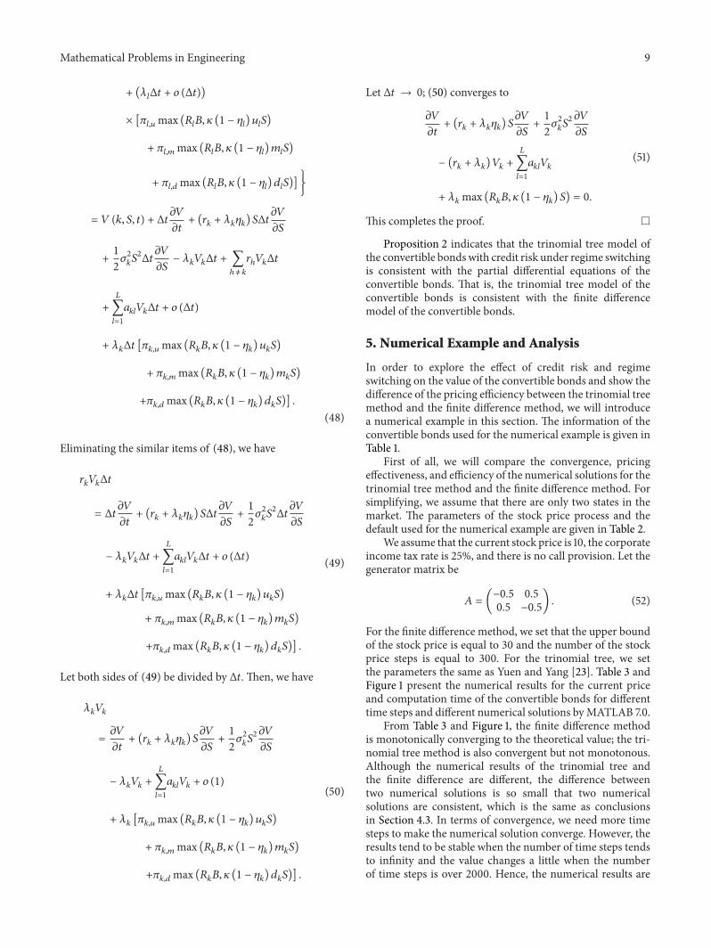
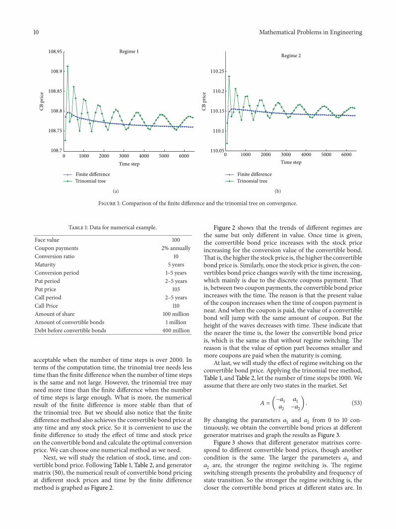
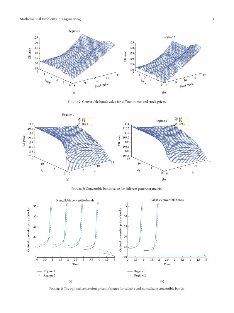
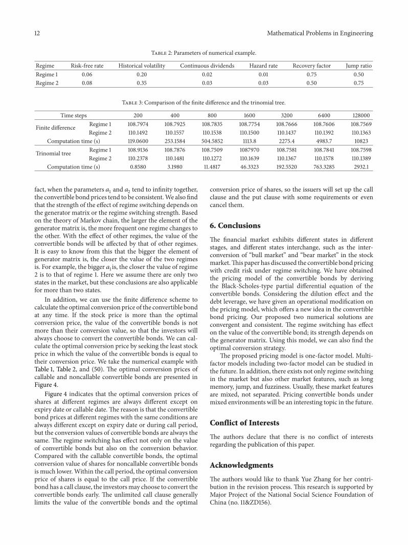