
Pricing Model for Convertible Bonds: A Mixed …...Pricing Model for Convertible Bonds: A Mixed...
16
East Asian Journal on Applied Mathematics Vol. 5, No. 3, pp. 222-237 doi: 10.4208/eajam.221214.240415a August 2015 Pricing Model for Convertible Bonds: A Mixed Fractional Brownian Motion with Jumps Jie Miao 1,2, ∗ and Xu Yang 1 1 School of Mathematics, Shandong University, Jinan, Shandong 250100, China. 2 Department of Mathematics, Changji College, Changji, Xinjiang 831100, China. Received 22 December 2014; Accepted (in revised version) 24 April 2015 Abstract. A mathematical model to price convertible bonds involving mixed fractional Brownian motion with jumps is presented. We obtain a general pricing formula using the risk neutral pricing principle and quasi-conditional expectation. The sensitivity of the price to changing various parameters is discussed. Theoretical prices from our jump mixed fractional Brownian motion model are compared with the prices predicted by traditional models. An empirical study shows that our new model is more acceptable. AMS subject classifications: 60J75, 60G22, 91G80 Key words: Mixed fractional Brownian motion, Poisson jump, convertible bond, empirical study. 1. Introduction A convertible bond is a complex financial product that enables the holder to exchange the bond for the issuer’s underlying stock in some specified circumstance. The charac- teristics of both bond and equity make the valuation of convertible bonds quite difficult. Indeed, the convertible bond trade is an emerging market, and it is important to consider more factors that influence convertible bond pricing than allowed for by existing pricing methods. Theoretical research on convertible bond pricing was initiated by Ingersoll [1], who applied the well known Black-Scholes-Merton options pricing model. Following his work, Brennan & Schwartz [2] used corporate value as the basic variable to price convertible bonds, and then took into account the uncertainty inherent in interest rates and also the possibility of senior debt in the firm’s capital structure [3]. Nyborg [4] considered the more complicated call and put features in convertible bond pricing under stochastic interest rates. In these ways, researchers have gradually added various factors to increase the accuracy of convertible bond pricing. ∗ Corresponding author. Email addresses: (J. Miao), (X. Yang) http://www.global-sci.org/eajam 222 c ⃝2015 Global-Science Press
Transcript of Pricing Model for Convertible Bonds: A Mixed …...Pricing Model for Convertible Bonds: A Mixed...
East Asian Journal on Applied Mathematics Vol. 5, No. 3, pp. 222-237doi: 10.4208/eajam.221214.240415a August 2015
Pricing Model for Convertible Bonds: A Mixed
Fractional Brownian Motion with Jumps
Jie Miao1,2,∗ and Xu Yang1
1 School of Mathematics, Shandong University, Jinan, Shandong 250100, China.2 Department of Mathematics, Changji College, Changji, Xinjiang 831100, China.
Received 22 December 2014; Accepted (in revised version) 24 April 2015
Abstract. A mathematical model to price convertible bonds involving mixed fractionalBrownian motion with jumps is presented. We obtain a general pricing formula usingthe risk neutral pricing principle and quasi-conditional expectation. The sensitivity ofthe price to changing various parameters is discussed. Theoretical prices from our jumpmixed fractional Brownian motion model are compared with the prices predicted bytraditional models. An empirical study shows that our new model is more acceptable.
AMS subject classifications: 60J75, 60G22, 91G80
Key words: Mixed fractional Brownian motion, Poisson jump, convertible bond, empirical study.
1. Introduction
A convertible bond is a complex financial product that enables the holder to exchange
the bond for the issuer’s underlying stock in some specified circumstance. The charac-
teristics of both bond and equity make the valuation of convertible bonds quite difficult.
Indeed, the convertible bond trade is an emerging market, and it is important to consider
more factors that influence convertible bond pricing than allowed for by existing pricing
methods.
Theoretical research on convertible bond pricing was initiated by Ingersoll [1], who
applied the well known Black-Scholes-Merton options pricing model. Following his work,
Brennan & Schwartz [2] used corporate value as the basic variable to price convertible
bonds, and then took into account the uncertainty inherent in interest rates and also the
possibility of senior debt in the firm’s capital structure [3]. Nyborg [4] considered the more
complicated call and put features in convertible bond pricing under stochastic interest rates.
In these ways, researchers have gradually added various factors to increase the accuracy of
convertible bond pricing.
∗Corresponding author. Email addresses: (J. Miao),(X. Yang)
http://www.global-sci.org/eajam 222 c⃝2015 Global-Science Press

Pricing Model for Convertible Bonds 223
The above articles all regard the price movement as a geometric Brownian motion.
However, many empirical studies demonstrate that the distributions of the logarithmic re-
turns on the financial asset usually exhibit self-similarity properties, heavy tails and long-
range dependence in both auto-correlations and cross-correlations, and volatility clustering
[5-10]. Indeed, the most common stochastic process that exhibits long-range dependence
is a fractional Brownian motion (FBM). Furthermore, an FBM produces a burstiness in the
sample path behaviour, an important aspect of financial time series. Consequently, it is nat-
ural to replace the Brownian motion with an FBM to make stochastic models more realistic
[11-15].
Classical Ito theory cannot be applied to an FBM, and defining an associated proper
stochastic integral is difficult [16]. A major difficulty is that an FBM is not semi-martingale,
so to take the long memory property into account it is reasonable to prefer a mixed frac-
tional Brownian motion (MFBM) in order to capture the price fluctuations of a financial
asset [17-18]. An MFBM is essentially a family of Gaussian processes in a linear combi-
nation of Brownian motion and FBM — a class of long memory processes with the Hurst
parameter H ∈ (1/2,1). The first work in economics using an MFBM is in Ref. [19], where
for H ∈ (3/4,1) it was proven that an MFBM is equivalent in law to a Brownian motion,
and hence financial markets driven by the MFBM is arbitrage-free. Recent additional ap-
plications have also been documented [20]. However, all of the above-mentioned earlier
research considered that the logarithmic returns of the underlying stock are independent
identically distributed normal random variables, whereas the empirical study of asset re-
turn indicates that discontinuities or jumps are an essential component of financial asset
price series [21-23]. Merton [24] proposed a jump-diffusion process involving a Poisson
jump, given the observed abnormal fluctuations in stock prices. Based on his theory, several
authors have modelled the price of a convertible bond as a Brownian motion with Poisson
jumps [25-27].
This article provides a theoretical, numerical and empirical contribution to the study of
convertible bonds. To capture jumps or discontinuities and account for the long memory
property, a combination of Poisson jumps and mixed fractional Brownian motion is used.
As in Ref. [19], we assume H ∈ (3/4,1) throughout, an assumption validated by many
previous empirical studies [20, 28]. Our jump mixed fractional Brownian motion (JMFBM)
model produces empirically observed distributions of stock price changes that are skewed,
leptokurtic, long memory and possess fatter tails than comparable normal distributions. A
JMFBM model to price convertible bonds has not been investigated before, and our new
model allows us to explore the sensitivities of the convertible bond price to changes in
various relevant parameters. Numerical experiments supplemented by an empirical study
indicate that our JMFBM model more closely predicts the actual market in convertible bonds
than any purely Brownian motion model.
The rest of the article is organized as follows. Some MFBM results are recalled in
Section 2, and we present the JMFBM pricing model for convertible bonds in Section 3.
Section 4 contains the sensitivity analysis for the convertible bond price. We numerically
compare our JMFBM model with traditional models in Section 5, and discuss the relation-
ship between the convertible bond price and the parameters of the Hurst and jump. In

224 J. Miao and X. Yang
Section 6, an empirical study shows that our model is more acceptable. Our concluding
remarks are in Section 7.
2. Preliminaries
We first recall some essential results — cf. also Refs. [22,29,30].
Definition 2.1. An MFBM with parameters a, b and H is a linear combination of Brownian
motion and FBM with Hurst parameter H, defined on the probability space (Ω,$ ,!) for
any t ∈ "+ by M Ht = aBt + bBH
t , where a and b are two real constants such that (a, b) =(0,0), Bt is a Brownian motion, BH
t is an FBM with Hurst parameter H ∈ (0,1), which is
independent of Bt .
Proposition 2.1. The MFBM M Ht satisfies the following properties:
(i) M Ht is a centred Gaussian process and not Markovian;
(ii) M Ht = 0, !-almost surely;
(iii) the covariance of M Ht (a, b) and M H
s (a, b) for any t, s ∈ "+ is given by
cov!
M Ht , M H
t
"
= a2 (t ∧ s) +b2
2
!
t2H + s2H − |t − s|2H"
, (2.1)
where ∧ denotes mins, t;(iv) the increments of M H
t (a, b) are stationary and mixed-self-similar for any h > 0:
M Hht(a, b) # M H
t
#
ah12 , bhH$
, (2.2)
where # means “to have the same law”;
(v) the increments of M Ht are positively correlated if 1/2< H < 1, uncorrelated if H = 1/2
and negatively correlated if 0< H < 1/2 ;
(vi) the increments of M Ht are long-range dependent if and only if H > 1/2;
(vii) for all t ∈ R+,
E%
(M Ht (a, b))n&
=
⎧
⎨
⎩
0 , n= 2l + 1 ,(2l)!
2l l!(a2 t + b2 t2H)l , n= 2l .
(2.3)
Lemma 2.1. For every t ∈ [0, T ], if σ,ϵ ∈ C then
$!%
eσ(BT+ϵBHT )|$t
&
= eσ(Bt+ϵBHt )+
σ2
2 (T−t)+σ2ϵ2
2 (T2H−t2H ) , (2.4)
where ! is a risk-neutral probability measure and $![·|$t] denotes the quasi-conditional ex-
pectation with respect to $t under the probability measure !.
Proof. The proof is similar to that of Lemma A.1. in Ref. [29] and so omitted here.
Pricing Model for Convertible Bonds 225
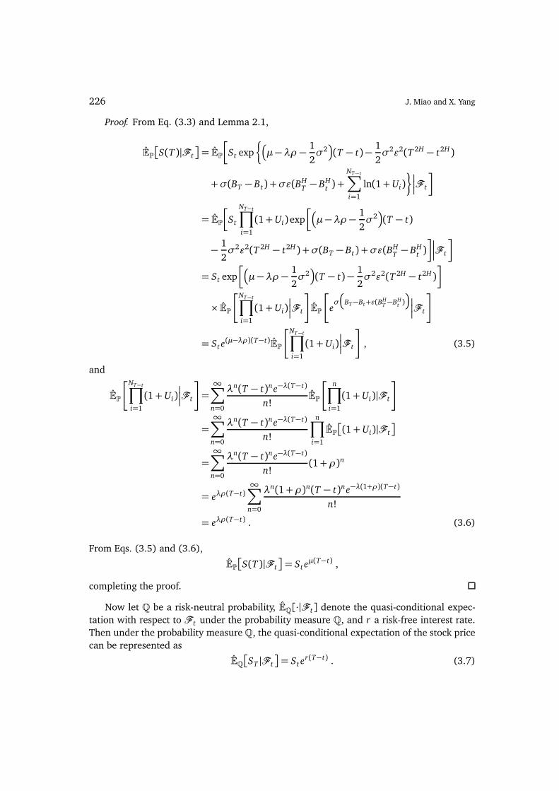
3. Pricing Model for Convertible Bonds in the JMFBM Environment
3.1. The JMFBM market
Consider a market consisting of one bond (a riskless asset) and one stock (a risky asset).
The price At of the bond evolves (for t ∈ [0, T ]) according to the differential equation and
initial price
dAt = rAt d t , A0 = 1 , (3.1)
where the interest rate r is assumed constant.
The price St of the stock is assumed to satisfy
dSt = St
%
(µ−λρ)d t +σ(dBt + ϵdBHt ) + UdNt
&
, S0 = S , (3.2)
where the drift µ and volatility σ are assumed constant, Bt is a Brownian motion, BHt is
a fractional Brownian motion with Hurst parameter H ∈ (3/4,1), Nt is a Poisson process
with intensity λ, U1, · · · , Un are jump sizes of the stock price (a sequence of independent
identically distributed random variables), ρ = E(U) and ln(1+ U) ∼ N (µU ,σU). All four
sources of randomness (the Brownian motion Bt , the fractional Brownian motion BHt , the
Poisson process Nt and the jump size U) are assumed to be independent.
We consider a probability space
!
Ω,$ , ($t )0≤t≤T ,!"
,
$t = σ[Bs; s ≤ t] ∨σ[BHs ; s ≤ t] ∨σ[N ((0, s]; s ≤ t] ∨σ[Ui , i ≥ 1] .
Since St satisfies Eq. (3.2), let yt = lnSt , using the I t o formula we get
ST = St exp
*
(µ−λρ − 1
2σ2)(T − t)− 1
2σ2ϵ2(T 2H − t2H)
+σ(BT − Bt) +σϵ(BHT − BH
t ) +
NT−t∑
i=1
ln(1+ Ui)
,
.
(3.3)
Theorem 3.1. For T ≥ t, the quasi-conditional expectation of the stock price is
$!%
S(T )|$t
&
= St eµ(T−t) . (3.4)
226 J. Miao and X. Yang
Proof. From Eq. (3.3) and Lemma 2.1,
$!%
S(T )|$t
&
= $!
*
St exp
-#
µ−λρ − 1
2σ2$
(T − t)− 1
2σ2ϵ2(T 2H − t2H )
+σ(BT − Bt) +σϵ(BHT − BH
t ) +
NT−t∑
i=1
ln(1+ Ui)
./
/
/$t
,
= $!
*
St
NT−t∏
i=1
(1+ Ui)exp
*#
µ−λρ− 1
2σ2$
(T − t)
− 1
2σ2ϵ2(T 2H − t2H) +σ(BT − Bt) +σϵ(B
HT − BH
t )
,/
/
/$t
,
= St exp
*#
µ−λρ − 1
2σ2$
(T − t)− 1
2σ2ϵ2(T 2H − t2H )
,
× $!1NT−t∏
i=1
(1+ Ui)/
/
/$t
2
$!
1
eσ
#
BT−Bt+ϵ(BHT −BH
t )
$
/
/
/$t
2
= St e(µ−λρ)(T−t)$!
1NT−t∏
i=1
(1+ Ui)
/
/
/$t
2
, (3.5)
and
$!
1NT−t∏
i=1
(1+ Ui)/
/
/$t
2
=
∞∑
n=0
λn(T − t)ne−λ(T−t)
n!$!
1
n∏
i=1
(1+ Ui)|$t
2
=
∞∑
n=0
λn(T − t)ne−λ(T−t)
n!
n∏
i=1
$!%
(1+ Ui)|$t
&
=
∞∑
n=0
λn(T − t)ne−λ(T−t)
n!(1+ρ)n
= eλρ(T−t)∞∑
n=0
λn(1+ρ)n(T − t)ne−λ(1+ρ)(T−t)
n!
= eλρ(T−t) . (3.6)
From Eqs. (3.5) and (3.6),
$!%
S(T )|$t
&
= St eµ(T−t) ,
completing the proof.
Now let % be a risk-neutral probability, $%[·|$t] denote the quasi-conditional expec-
tation with respect to $t under the probability measure %, and r a risk-free interest rate.
Then under the probability measure %, the quasi-conditional expectation of the stock price
can be represented as
$%%
ST |$t
&
= St er(T−t) . (3.7)
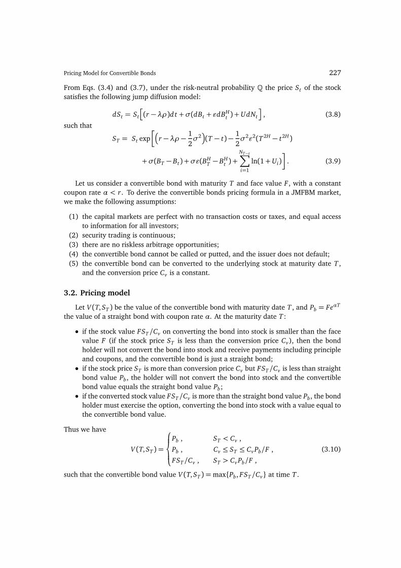
Pricing Model for Convertible Bonds 227
From Eqs. (3.4) and (3.7), under the risk-neutral probability % the price St of the stock
satisfies the following jump diffusion model:
dSt = St
3
(r −λρ)d t +σ(dBt + ϵdBHt ) + UdNt
4
, (3.8)
such that
ST = St exp
*#
r − λρ− 1
2σ2$
(T − t)− 1
2σ2ϵ2(T 2H − t2H )
+σ(BT − Bt) +σϵ(BHT − BH
t ) +
NT−t∑
i=1
ln(1+ Ui)
,
. (3.9)
Let us consider a convertible bond with maturity T and face value F , with a constant
coupon rate α < r. To derive the convertible bonds pricing formula in a JMFBM market,
we make the following assumptions:
(1) the capital markets are perfect with no transaction costs or taxes, and equal access
to information for all investors;
(2) security trading is continuous;
(3) there are no riskless arbitrage opportunities;
(4) the convertible bond cannot be called or putted, and the issuer does not default;
(5) the convertible bond can be converted to the underlying stock at maturity date T ,
and the conversion price Cv is a constant.
3.2. Pricing model
Let V (T,ST ) be the value of the convertible bond with maturity date T , and Pb = FeαT
the value of a straight bond with coupon rate α. At the maturity date T :
• if the stock value FST/Cv on converting the bond into stock is smaller than the face
value F (if the stock price ST is less than the conversion price Cv), then the bond
holder will not convert the bond into stock and receive payments including principle
and coupons, and the convertible bond is just a straight bond;
• if the stock price ST is more than conversion price Cv but FST/Cv is less than straight
bond value Pb, the holder will not convert the bond into stock and the convertible
bond value equals the straight bond value Pb;
• if the converted stock value FST/Cv is more than the straight bond value Pb, the bond
holder must exercise the option, converting the bond into stock with a value equal to
the convertible bond value.
Thus we have
V (T,ST ) =
⎧
⎪
⎨
⎪
⎩
Pb , ST < Cv ,
Pb , Cv ≤ ST ≤ Cv Pb/F ,
FST/Cv , ST > Cv Pb/F ,
(3.10)
such that the convertible bond value V (T,ST ) =maxPb, FST/Cv at time T .
228 J. Miao and X. Yang
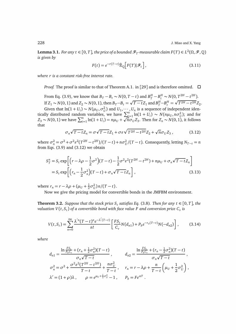
Lemma 3.1. For any t ∈ [0, T ], the price of a bounded$T -measurable claim F(T ) ∈ L2(Ω,$ ,%)is given by
F(t) = e−r(T−t)$%3
F(T )|$t
4
, (3.11)
where r is a constant risk-free interest rate.
Proof. The proof is similar to that of Theorem A.1. in [29] and is therefore omitted.
From Eq. (3.9), we know that BT − Bt ∼ N (0, T − t) and BHT − BH
t ∼ N (0, T 2H − t2H ).
If Z1 ∼ N (0,1) and Z2 ∼ N (0,1), then BT−Bt =.
T − tZ1 and BHT −BH
t =.
T 2H − t2H Z2.
Given that ln(1+ Ui) ∼ N (µU ,σ2U) and U1, · · · , Un is a sequence of independent iden-
tically distributed random variables, we have∑n
i=1 ln(1 + Ui) ∼ N (nµU , nσ2U); and for
Z3 ∼ N (0,1) we have∑n
i=1 ln(1+ Ui) = nµU +.
nσU Z3. Then for Zn ∼ N (0,1), it follows
that
σn
.T − tZn = σ
.T − tZ1 +σϵ7
T 2H − t2H Z2 +.
nσU Z3 , (3.12)
where σ2n = σ
2+σ2ϵ2(T 2H − t2H)/(T − t)+ nσ2U/(T − t). Consequently, letting NT−t = n
from Eqs. (3.9) and (3.12) we obtain
SnT = St exp
*#
r −λρ − 1
2σ2$
(T − t)− 1
2σ2ϵ2(T 2H − t2H ) + nµU +σn
.T − tZn
,
= St exp
*#
rn −1
2σ2
n
$
(T − t) +σn
.T − tZn
,
, (3.13)
where rn = r −λρ + (µU +12σ
2U)n/(T − t) .
Now we give the pricing model for convertible bonds in the JMFBM environment.
Theorem 3.2. Suppose that the stock price St satisfies Eq. (3.8). Then for any t ∈ [0, T ], the
valuation V (t,St ) of a convertible bond with face value F and conversion price Cv is
V (t,St ) =
∞∑
n=0
λ′n(T − t)ne−λ
′(T−t)
n!
*
FSt
Cv
N (dn1) + Pbe−rn(T−t)N (−dn2)
,
, (3.14)
where
dn1 =ln
FSt
PbCv+ (rn +
12σ
2n)(T − t)
σn
.T − t
, dn2 =ln
FSt
PbCv+ (rn − 1
2σ2n)(T − t)
σn
.T − t
,
σ2n = σ
2 +σ2ϵ2(T 2H − t2H)
T − t+
nσ2U
T − t, rn = r −λρ+ n
T − t
8
µU +1
2σ2
U
9
,
λ′ = (1+ρ)λ , ρ = eµU+12σ
2U − 1 , Pb = FeαT .
Pricing Model for Convertible Bonds 229
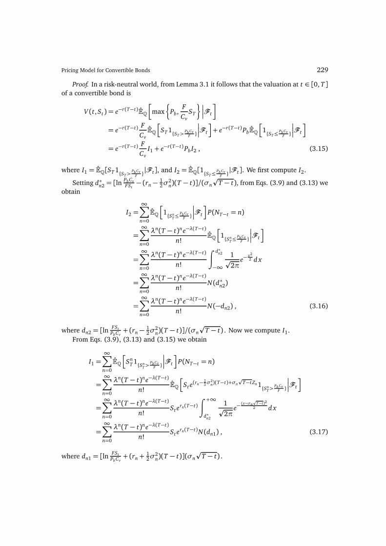
Proof. In a risk-neutral world, from Lemma 3.1 it follows that the valuation at t ∈ [0, T ]
of a convertible bond is
V (t,St ) = e−r(T−t)$%
*
max
-
Pb,F
Cv
ST
./
/
/$t
,
= e−r(T−t) F
Cv
$%:
ST 1ST>PbCv
F
/
/
/$t
;
+ e−r(T−t)Pb$%:
1ST≤PbCv
F
/
/
/$t
;
= e−r(T−t) F
Cv
I1 + e−r(T−t)PbI2 , (3.15)
where I1 = $%[ST 1ST>PbCv
F |$t], and I2 = $%[1ST≤
PbCvF |$t]. We first compute I2.
Setting d∗n2 = [lnPbCv
FSt− (rn − 1
2σ2n)(T − t)]/(σn
.T − t), from Eqs. (3.9) and (3.13) we
obtain
I2 =
∞∑
n=0
$%:
1SnT≤
PbCvF
/
/
/$t
;
P(NT−t = n)
=
∞∑
n=0
λn(T − t)ne−λ(T−t)
n!$%:
1SnT≤
PbCvF
/
/
/$t
;
=
∞∑
n=0
λn(T − t)ne−λ(T−t)
n!
∫ d∗n2
−∞
1.2π
e−x2
2 d x
=
∞∑
n=0
λn(T − t)ne−λ(T−t)
n!N (d∗n2)
=
∞∑
n=0
λn(T − t)ne−λ(T−t)
n!N (−dn2) , (3.16)
where dn2 = [lnFSt
PbCv+ (rn − 1
2σ2n)(T − t)]/(σn
.T − t) . Now we compute I1.
From Eqs. (3.9), (3.13) and (3.15) we obtain
I1 =
∞∑
n=0
$%:
SnT 1Sn
T>PbCv
F
/
/
/$t
;
P(NT−t = n)
=
∞∑
n=0
λn(T − t)ne−λ(T−t)
n!$%:
St e(rn− 1
2σ2n)(T−t)+σn
.T−tZn 1Sn
T>PbCv
F
/
/
/$t
;
=
∞∑
n=0
λn(T − t)ne−λ(T−t)
n!St e
rn(T−t)
∫ +∞
d∗n2
1.2π
e−(x−σn
.T−t)2
2 d x
=
∞∑
n=0
λn(T − t)ne−λ(T−t)
n!St e
rn(T−t)N (dn1) , (3.17)
where dn1 = [lnFSt
PbCv+ (rn +
12σ
2n)(T − t)](σn
.T − t) .
230 J. Miao and X. Yang
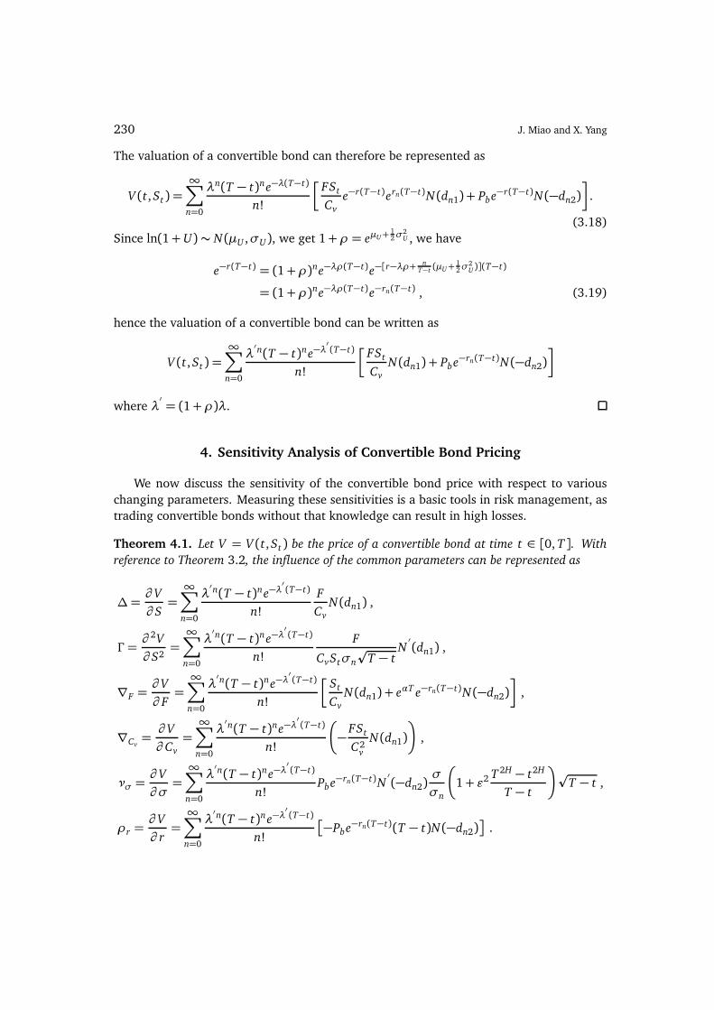
The valuation of a convertible bond can therefore be represented as
V (t,St ) =
∞∑
n=0
λn(T − t)ne−λ(T−t)
n!
*
FSt
Cv
e−r(T−t)ern(T−t)N (dn1) + Pbe−r(T−t)N (−dn2)
,
.
(3.18)
Since ln(1+ U)∼ N (µU ,σU), we get 1+ρ = eµU+12σ
2U , we have
e−r(T−t) = (1+ρ)ne−λρ(T−t)e−[r−λρ+n
T−t (µU+12σ
2U )](T−t)
= (1+ρ)ne−λρ(T−t)e−rn(T−t) , (3.19)
hence the valuation of a convertible bond can be written as
V (t,St ) =
∞∑
n=0
λ′n(T − t)ne−λ
′(T−t)
n!
*
FSt
Cv
N (dn1) + Pbe−rn(T−t)N (−dn2)
,
where λ′= (1+ρ)λ.
4. Sensitivity Analysis of Convertible Bond Pricing
We now discuss the sensitivity of the convertible bond price with respect to various
changing parameters. Measuring these sensitivities is a basic tools in risk management, as
trading convertible bonds without that knowledge can result in high losses.
Theorem 4.1. Let V = V (t,St ) be the price of a convertible bond at time t ∈ [0, T ]. With
reference to Theorem 3.2, the influence of the common parameters can be represented as
∆=∂ V
∂ S=
∞∑
n=0
λ′n(T − t)ne−λ
′(T−t)
n!
F
Cv
N (dn1) ,
Γ =∂ 2V
∂ S2=
∞∑
n=0
λ′n(T − t)ne−λ
′(T−t)
n!
F
CvStσn
.T − t
N′(dn1) ,
∇F =∂ V
∂ F=
∞∑
n=0
λ′n(T − t)ne−λ
′(T−t)
n!
*
St
Cv
N (dn1) + eαT e−rn(T−t)N (−dn2)
,
,
∇Cv=∂ V
∂ Cv
=
∞∑
n=0
λ′n(T − t)ne−λ
′(T−t)
n!
=
− FSt
C2v
N (dn1)
>
,
νσ =∂ V
∂ σ=
∞∑
n=0
λ′n(T − t)ne−λ
′(T−t)
n!Pbe−rn(T−t)N
′(−dn2)
σ
σn
=
1+ ϵ2 T 2H − t2H
T − t
>.T − t ,
ρr =∂ V
∂ r=
∞∑
n=0
λ′n(T − t)ne−λ
′(T−t)
n!
%
−Pbe−rn(T−t)(T − t)N (−dn2)&
.

Pricing Model for Convertible Bonds 231
Proof. The proof is immediate from the chain rule of a compound function.
Remark 4.1. From Theorem 4.1, we can easily deduce that ∆ ≥ 0,∇F ≥ 0, νσ ≥ 0, Γ ≥ 0,
∇CV≤ 0 and ρr ≤ 0, so the valuation of a convertible bond is an increasing function of St ,
F and σ, and a decreasing function of Cv and ρr .
Theorem 4.2. Suppose V = V (t,St) is the price of a convertible bond at time t ∈ [0, T ].
From Theorem 3.2, the influence of the Hurst parameter can be expressed as
∂ V
∂ H=
∞∑
n=0
λ′n(T − t)ne−λ
′(T−t)
n!Pbe−rn(T−t)N
′(−dn2)
σ2ϵ2
σn
.T − t
(T 2H ln T − t2H ln t) . (4.1)
Remark 4.2. From Theorem 4.2, we can easily deduce that ∂ V/∂ H ≥ 0, so the valuation
of a convertible bond will increase with increasing Hurst parameter.
Theorem 4.3. Let V = V (t,St ) be the price of a convertible bond at time t ∈ [0, T ]. From
Theorem 3.2, the influence of the jump parameters can be represented as
∂ V
∂ λ=
∞∑
n=0
λ′n(T − t)ne−λ
′(T−t)
n!(1+ρ)? n
λ′− (T − t)@*
FSt
Cv
N (dn1) + Pbe−rn(T−t)N (−dn2)
,
+
∞∑
n=0
λ′n(T − t)ne−λ
′(T−t)
n!Pbe−rn(T−t)ρ(T − t)N (−dn2) ,
∂ V
∂ µU
=
∞∑
n=0
λ′n(T − t)ne−λ
′(T−t)
n!λeµU+
12σ
2U
? n
λ′− (T − t)@*
FSt
Cv
N (dn1) + Pbe−rn(T−t)N (−dn2)
,
+
∞∑
n=0
λ′n(T − t)ne−λ
′(T−t)
n!Pbe−rn(T−t):?
λeµU+12σ
2U − n
T − t
@
(T − t)N (−dn2);
,
∂ V
∂ σU
=
∞∑
n=0
λ′n(T − t)ne−λ
′(T−t)
n!λσU eσU+
12σ
2U
? n
λ′− (T − t)@*
FSt
Cv
N (dn1) +Pbe−rn(T−t)N (−dn2)
,
+
∞∑
n=0
λ′n(T − t)ne−λ
′(T−t)
n!Pbe−rn(T−t):?
λσU eµU+12σ
2U − nσU
T − t
@
(T − t)N (−dn2)
+nσU
σn
.T − t
N′(−dn2)
A
,
Proof. The proof is again immediate.
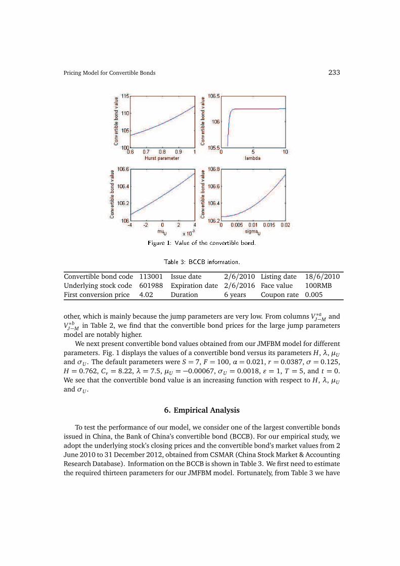
Fig. 1 intuitively displays the influence of the jump parameters on the valuation of the
convertible bond.
232 J. Miao and X. Yang
Model α r σ F Cv T t H ϵ λ µU σU
BM 0.021 0.0387 0.125 100 8.22 5 0
FBM 0.021 0.0387 0.125 100 8.22 5 0 0.762
MFBM 0.021 0.0387 0.125 100 8.22 5 0 0.762 1
J MBM a 0.021 0.0387 0.125 100 8.22 5 0 0.762 1 1.5 0.00067 0.0012
J MBM b 0.021 0.0387 0.125 100 8.22 5 0 0.762 1 7.5 -0.00067 0.0018
S VB−M VF−M VM−M V ∗ aJ−M V ∗ b
J−M
5 92.1919 92.4439 95.9998 96.0058 96.0128
6 94.2145 95.5998 100.3687 100.4107 100.4225
7 98.4865 100.8985 106.2863 106.2901 106.2963
8 105.1724 108.0915 113.5531 113.5629 113.5832
9 113.8785 116.7764 121.9306 121.9526 122.0285
10 124.0144 126.5580 131.1913 131.2691 131.2957∗The maximum number of iterations is 100.
aThe parameters for this calculations are in the fourth line of Table 1.bThe parameters for calculations are in the fifth line of Table 1.
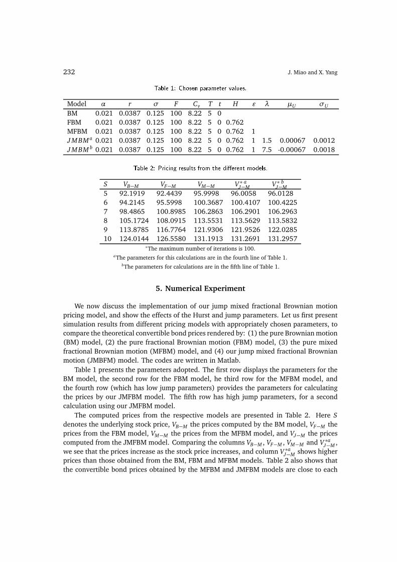
5. Numerical Experiment
We now discuss the implementation of our jump mixed fractional Brownian motion
pricing model, and show the effects of the Hurst and jump parameters. Let us first present
simulation results from different pricing models with appropriately chosen parameters, to
compare the theoretical convertible bond prices rendered by: (1) the pure Brownian motion
(BM) model, (2) the pure fractional Brownian motion (FBM) model, (3) the pure mixed
fractional Brownian motion (MFBM) model, and (4) our jump mixed fractional Brownian
motion (JMBFM) model. The codes are written in Matlab.
Table 1 presents the parameters adopted. The first row displays the parameters for the
BM model, the second row for the FBM model, he third row for the MFBM model, and
the fourth row (which has low jump parameters) provides the parameters for calculating
the prices by our JMFBM model. The fifth row has high jump parameters, for a second
calculation using our JMFBM model.
The computed prices from the respective models are presented in Table 2. Here S
denotes the underlying stock price, VB−M the prices computed by the BM model, VF−M the
prices from the FBM model, VM−M the prices from the MFBM model, and VJ−M the prices
computed from the JMFBM model. Comparing the columns VB−M , VF−M , VM−M and V ∗aJ−M ,
we see that the prices increase as the stock price increases, and column V ∗aJ−M shows higher
prices than those obtained from the BM, FBM and MFBM models. Table 2 also shows that
the convertible bond prices obtained by the MFBM and JMFBM models are close to each
Pricing Model for Convertible Bonds 233
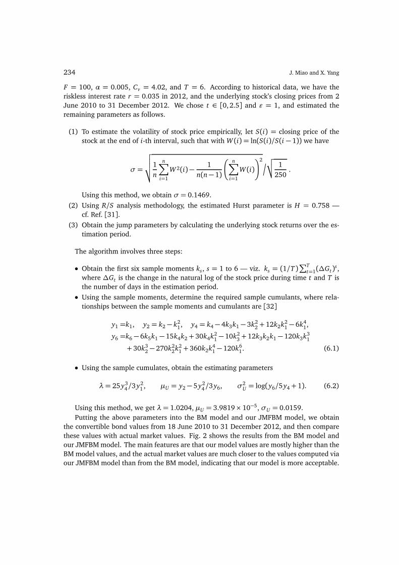
Convertible bond code 113001 Issue date 2/6/2010 Listing date 18/6/2010
Underlying stock code 601988 Expiration date 2/6/2016 Face value 100RMB
First conversion price 4.02 Duration 6 years Coupon rate 0.005
other, which is mainly because the jump parameters are very low. From columns V ∗aJ−M and
V ∗bJ−M in Table 2, we find that the convertible bond prices for the large jump parameters
model are notably higher.
We next present convertible bond values obtained from our JMFBM model for different
parameters. Fig. 1 displays the values of a convertible bond versus its parameters H, λ, µU
and σU . The default parameters were S = 7, F = 100, α = 0.021, r = 0.0387, σ = 0.125,
H = 0.762, Cv = 8.22, λ = 7.5, µU = −0.00067, σU = 0.0018, ϵ = 1, T = 5, and t = 0.
We see that the convertible bond value is an increasing function with respect to H, λ, µU
and σU .
6. Empirical Analysis
To test the performance of our model, we consider one of the largest convertible bonds
issued in China, the Bank of China’s convertible bond (BCCB). For our empirical study, we
adopt the underlying stock’s closing prices and the convertible bond’s market values from 2
June 2010 to 31 December 2012, obtained from CSMAR (China Stock Market & Accounting
Research Database). Information on the BCCB is shown in Table 3. We first need to estimate
the required thirteen parameters for our JMFBM model. Fortunately, from Table 3 we have
234 J. Miao and X. Yang
F = 100, α = 0.005, Cv = 4.02, and T = 6. According to historical data, we have the
riskless interest rate r = 0.035 in 2012, and the underlying stock’s closing prices from 2
June 2010 to 31 December 2012. We chose t ∈ [0,2.5] and ϵ = 1, and estimated the
remaining parameters as follows.
(1) To estimate the volatility of stock price empirically, let S(i) = closing price of the
stock at the end of i-th interval, such that with W (i) = ln(S(i)/S(i − 1)) we have
σ =
√
√
√
√1
n
n∑
i=1
W 2(i)− 1
n(n− 1)
E
n∑
i=1
W (i)
F2G
√
√ 1
250.
Using this method, we obtain σ = 0.1469.
(2) Using R/S analysis methodology, the estimated Hurst parameter is H = 0.758 —
cf. Ref. [31].
(3) Obtain the jump parameters by calculating the underlying stock returns over the es-
timation period.
The algorithm involves three steps:
• Obtain the first six sample moments ks, s = 1 to 6 — viz. ks = (1/T )∑T
t=1(∆Gt)s,
where ∆Gt is the change in the natural log of the stock price during time t and T is
the number of days in the estimation period.
• Using the sample moments, determine the required sample cumulants, where rela-
tionships between the sample moments and cumulants are [32]
y1 =k1, y2 = k2 − k21, y4 = k4 − 4k3k1 − 3k2
2 + 12k2k21 − 6k4
1,
y6 =k6 − 6k5k1 − 15k4k2 + 30k4k21 − 10k2
3 + 12k3k2k1 − 120k3k31
+ 30k32 − 270k2
2k21 + 360k2k4
1 − 120k61. (6.1)
• Using the sample cumulates, obtain the estimating parameters
λ= 25y34/3y2
1 , µU = y2 − 5y24/3y6, σ2
U = log(y6/5y4 + 1). (6.2)
Using this method, we get λ= 1.0204, µU = 3.9819× 10⁻⁵, σU = 0.0159.
Putting the above parameters into the BM model and our JMFBM model, we obtain
the convertible bond values from 18 June 2010 to 31 December 2012, and then compare
these values with actual market values. Fig. 2 shows the results from the BM model and
our JMFBM model. The main features are that our model values are mostly higher than the
BM model values, and the actual market values are much closer to the values computed via
our JMFBM model than from the BM model, indicating that our model is more acceptable.

Pricing Model for Convertible Bonds 235
7. Conclusion
Convertible bonds are popular financial derivatives, with an essential role in the Chi-
nese financial market. Pricing them efficiently and accurately is very important, in both
theory and practice. To capture the long memory and discontinuous property, this article
focuses on the problem of pricing convertible bonds in a jump mixed fractional Brownian
environment. After formulating our convertible bond pricing model, we discussed the pric-
ing formula for the mixed fractional Brownian motion with jumps involved. We compared
theoretical values obtained from other available valuation models with the values from our
model in a numerical simulation. Finally, we presented an empirical study using actual
data from the Chinese convertible bond market, which showed that our JMFBM model is
more acceptable.
Acknowledgments
This research is partially supported by the National Natural Science Foundations of
China under grant numbers 91130003 and 11171189.
References
[1] J.E. Ingersoll Jr., A contingent-claims valuation of convertible securities, J. Financial Economics4, 289-321 (1977).
[2] M.J. Brennan and E.S. Schwartz, Convertible bonds: Valuation and optimal strategies for calland conversion, J. Finance 32, 1699-1715 (1977).
236 J. Miao and X. Yang
[3] M.J. Brennan and E.S. Schwartz, Analyzing convertible bonds, J. Financial and QuantitativeAnalysis 15, 907-929 (1980).
[4] K.G. Nyborg, The use and pricing of convertible bonds, Applied Mathematical Finance 3, 167-190 (1996).
[5] R.N. Mantegna and H.E. Stanley, Turbulence and financial markets, Nature 383, 587-588(1996).
[6] D.O. Cajueiro and B.M. Tabak, Long-range dependence and multifractality in the term structureof LIBOR interest rates, Physica A 373, 603-614 (2007).
[7] S. Kang and S.M. Yoon, Long memory features in the high frequency data of the Korean stockmarket, Physica A 387, 5189-5196 (2008).
[8] Y. Wang, Y. Wei and C. Wu, Cross-correlations between Chinese A-share and B-share markets,Physica A 389, 5468-5478 (2010).
[9] Z. Ding, C.W.J. Granger and R.F. Engle, A long memory property of stock market returns and anew model, J. Empirical Finance 1, 83-106 (1993).
[10] Y. Liu, P. Gopikrishnan, P. Cizeau, M. Meyer, C. Peng and H.E. Stanley, The statistical propertiesof the volatility of price fluctuations, Phys. Rev. E 60, 1390-1400 (1999).
[11] C. Necula, Option pricing in a fractional Brownian motion environment, available at SSRN1286833 (2002).
[12] L. Lv, F. Ren and W. Qiu, The application of fractional derivatives in stochastic models driven byfractional Brownian motion, Physica A 389, 4809-4818 (2010).
[13] X. Wang, Scaling and long range dependence in option pricing, IV: pricing European optionswith transaction costs under the multifractional Black-Scholes model, Physica A 389, 789-796(2010).
[14] X. Wang, M. Wu, Z. Zhou and W. Jing, Pricing European option with transaction costs under thefractional long memory stochastic volatility model, Physica A 391, 1469-1480 (2012).
[15] M. Shen, Convertible bond pricing in fractional brownian motion environment, J. Anhui Uni-versity of Technology and Science 25, 72-74 (2010).
[16] S. Lin, Stochastic analysis of fractional Brownian motion, Stochastics and Stochastic Reports55, 121-140 (1995).
[17] Y. Mishura, Stochastic Calculus for Fractional Brownian Motions and Related Processes, SpringerVerlag, Berlin (2008).
[18] L. Li, J. Hu, Y. Chen and Y. Zhang, PCA based Hurst exponent estimator for fbm signals underdisturbances, IEEE Trans. Signal Processing 57, 2840-2846 (2009).
[19] P. Cheridito, Mixed fractional Brownian motion, Bernoulli 7, 913-934 (2001).[20] M. Zili, On the mixed fractional Brownian motion, J. Applied Math. and Stochastic Analysis
2006,1-9 (2006).[21] M. Chernov, A.R. Gallant, E. Ghysels and G. Tauchen, Alternative models for stock price dynam-
ics. J. Econometrics 116, 225-257 (2003).[22] B. Eraker, Do stock prices and volatility jump? Reconciling evidence from spot and option prices.
J. Finance 59, 1367-1403 (2004).[23] J. Pan, The jump-risk premia implicit in options: evidence from an integrated time-series study.
J. Financial Economics 63, 3-50 (2002).[24] R. Merton, Option pricing when underlying stock returns are discontinuous, J. Financial Eco-
nomics 3,125-144 (1976).[25] M. Davis and F.R. Lischka, Convertible bonds with market risk and credit risk, Working Paper,
Tokyo-Mitsubishi International (1999).[26] P.V. Gapeev and C. Kuhn, Perpetual convertible bonds in jump diffusion models, Statistics and
Decision 23, 15-31 (2005).

Pricing Model for Convertible Bonds 237
[27] H. Hua and X. Cheng, Pricing convertible bond based on the jump-diffusion process, Applicationof Statistics and Management 28, 347-351 (2009).
[28] C. Bender, T. Sottinen and E. Valkeila, Pricing by hedging and no-arbitrage beyond semimartin-gales, Finance Stochastics 12, 441-468 (2008).
[29] W. Xiao, W. Zhang, X. Zhang and Y. Wang, Pricing model for equity warrants in a mixed frac-tional Brownian environment and its algorithm, Physica A 391, 6418-6431 (2012).
[30] F. Shokrollahi and A. Kilicman, Pricing currency option in a mixed fractional Brownian motionwith jumps environment, Mathematical Problems in Engineering 2014, 1-13 (2014).
[31] L. He and W. Qian, A Monte Carlo simulation to the performance of the R/S and V/S methodstatistical revisit and real world application, Physica A 391, 3770-3782 (2012).
[32] M. Kendall and A. Stuart, The Advanced Theory of Statistics, Macmillan, New York (1977).