Research Article Equilibrium Point Bifurcation and...

Research ArticleEquilibrium Point Bifurcation and Singularity Analysis ofHH Model with Constraint

Xinhe Zhu1,2 and Zhiqiang Wu1

1 Department of Mechanics, School of Mechanical Engineering, Tianjin University, Tianjin 300072, China2Department of Mathematics, School of Science, Tianjin Polytechnic University, Tianjin 300387, China

Correspondence should be addressed to Zhiqiang Wu; [email protected]

Received 10 April 2014; Accepted 23 June 2014; Published 7 July 2014

Academic Editor: Rehana Naz

Copyright © 2014 X. Zhu and Z. Wu. This is an open access article distributed under the Creative Commons Attribution License,which permits unrestricted use, distribution, and reproduction in any medium, provided the original work is properly cited.

We present the equilibrium point bifurcation and singularity analysis of HH model with constraints. We investigate the effect ofconstraints and parameters on the type of equilibrium point bifurcation. HH model with constraints has more transition sets. TheMatcont toolbox software environment was used for analysis of the bifurcation points in conjunction withMatlab.We also illustratethe stability of the equilibrium points.

1. Introduction

The Hodgkin-Huxley nonlinear model (HH) [1] is one ofthe biggest challenges in the life science in the near history.HH quantitatively describes the electrical excitations of squidgiant axon. Under the HH formalism, many mathematicalmodels (HH-type) for diverse neurons are established [2–5]. A bifurcation is a qualitative change in the behaviorof a nonlinear dynamical system as its parameters passthrough critical values [6]. The study of bifurcations inneural models is important to understand the dynamicalorigin of many neurons and the organization of behavior.Many studies have been done on the bifurcation analysisof HH model. Guckenheimer and Labouriau [7] give thedetailed bifurcation diagrams ofHHmodel in two-parameterspace of 𝐼 and 𝑉K. Bedrov reveals the possible bifurcationswith changes of 𝑔Na and 𝑔K, representing the maximalconductance of sodium and potassium, respectively [8, 9].The global structure of bifurcations in multiple-parameterspace of the HH model is examined [10], and the detailsof the degenerate Hopf bifurcations are analyzed using thesingularity theoretic approach [11]. Singularity theory offersan extremely useful approach to bifurcation problems [12].The aim of this paper is to illustrate how constraints andparameters affect the dynamics of HH model. In the firstattempt we choose 𝐼 as bifurcation parameter, 𝑔K, 𝑔𝐿 as

unfolding parameters, and we restrict 𝑉 > 0; then we usethe singularity theory of bifurcations and the computingmethod of bifurcations with constraint to obtain the newconstraint transition sets. Secondly, using the above results,we investigate the effect of constraint and parameters on thetype of equilibrium point bifurcation, and we also illustratethe stability of the equilibrium points.

2. Hodgkin-Huxley Equations

TheHH comprises the following differential equations:

𝑑𝑉

𝑑𝑡=

1

𝐶𝑀

[𝐼 − 𝑔Na𝑚3ℎ (𝑉 − 𝑉Na)

−𝑔K𝑛4(𝑉 − 𝑉K) − 𝑔𝑙 (𝑉 − 𝑉

𝑙)] ,

𝑑𝑚

𝑑𝑡= 𝛼𝑚 (1 − 𝑚) − 𝛽𝑚𝑚,

𝑑ℎ

𝑑𝑡= 𝛼ℎ (1 − ℎ) − 𝛽ℎℎ,

𝑑𝑛

𝑑𝑡= 𝛼𝑛 (1 − 𝑛) − 𝛽𝑛𝑛.

(1)

𝑉 represents the membrane potential. 0 ≤ 𝑚 ≤ 1 and0 ≤ ℎ ≤ 1 are the gating variables representing activation

Hindawi Publishing CorporationAbstract and Applied AnalysisVolume 2014, Article ID 545236, 8 pageshttp://dx.doi.org/10.1155/2014/545236

2 Abstract and Applied Analysis

gL

gK

25

20

15

10

5

0

0 2 4 6 8 10

Hysteresis set (H)Constrained hysteresis set (HI)Constrained double limit point set (DLI)

1

23

4

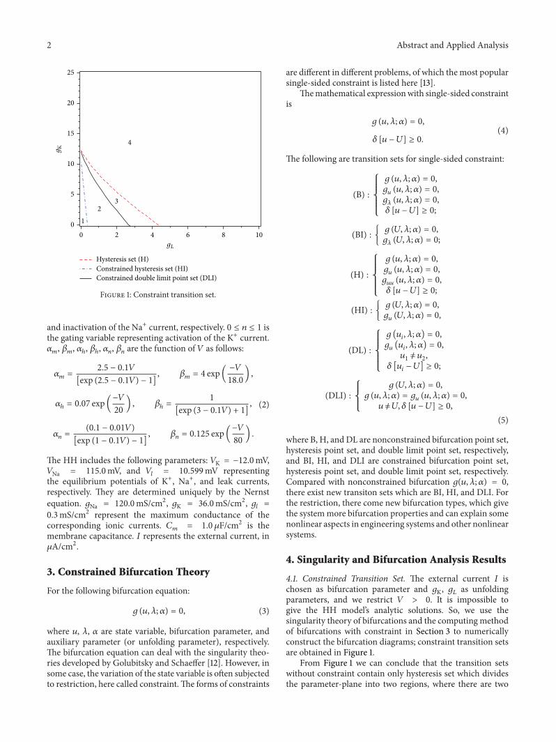
Figure 1: Constraint transition set.

and inactivation of the Na+ current, respectively. 0 ≤ 𝑛 ≤ 1 isthe gating variable representing activation of the K+ current.𝛼𝑚, 𝛽𝑚, 𝛼ℎ, 𝛽ℎ, 𝛼𝑛, 𝛽𝑛are the function of 𝑉 as follows:

𝛼𝑚=

2.5 − 0.1𝑉

[exp (2.5 − 0.1𝑉) − 1], 𝛽

𝑚= 4 exp( −𝑉

18.0) ,

𝛼ℎ= 0.07 exp(−𝑉

20) , 𝛽

ℎ=

1

[exp (3 − 0.1𝑉) + 1],

𝛼𝑛=

(0.1 − 0.01𝑉)

[exp (1 − 0.1𝑉) − 1], 𝛽

𝑛= 0.125 exp(−𝑉

80) .

(2)

The HH includes the following parameters: 𝑉K = −12.0mV,𝑉Na = 115.0mV, and 𝑉

𝑙= 10.599mV representing

the equilibrium potentials of K+, Na+, and leak currents,respectively. They are determined uniquely by the Nernstequation. 𝑔Na = 120.0mS/cm2, 𝑔K = 36.0mS/cm2, 𝑔

𝑙=

0.3mS/cm2 represent the maximum conductance of thecorresponding ionic currents. 𝐶

𝑚= 1.0 𝜇F/cm2 is the

membrane capacitance. 𝐼 represents the external current, in𝜇A/cm2.

3. Constrained Bifurcation Theory

For the following bifurcation equation:

𝑔 (𝑢, 𝜆; 𝛼) = 0, (3)

where 𝑢, 𝜆, 𝛼 are state variable, bifurcation parameter, andauxiliary parameter (or unfolding parameter), respectively.The bifurcation equation can deal with the singularity theo-ries developed by Golubitsky and Schaeffer [12]. However, insome case, the variation of the state variable is often subjectedto restriction, here called constraint.The forms of constraints

are different in different problems, of which themost popularsingle-sided constraint is listed here [13].

Themathematical expressionwith single-sided constraintis

𝑔 (𝑢, 𝜆; 𝛼) = 0,

𝛿 [𝑢 − 𝑈] ≥ 0.

(4)

The following are transition sets for single-sided constraint:

(B) :{{{

{{{

{

𝑔 (𝑢, 𝜆; 𝛼) = 0,

𝑔𝑢 (𝑢, 𝜆; 𝛼) = 0,

𝑔𝜆 (𝑢, 𝜆; 𝛼) = 0,

𝛿 [𝑢 − 𝑈] ≥ 0;

(BI) : { 𝑔 (𝑈, 𝜆; 𝛼) = 0,

𝑔𝜆 (𝑈, 𝜆; 𝛼) = 0;

(H) :{{{

{{{

{

𝑔 (𝑢, 𝜆; 𝛼) = 0,

𝑔𝑢 (𝑢, 𝜆; 𝛼) = 0,

𝑔𝑢𝑢 (𝑢, 𝜆; 𝛼) = 0,

𝛿 [𝑢 − 𝑈] ≥ 0;

(HI) : { 𝑔 (𝑈, 𝜆; 𝛼) = 0,

𝑔𝑢 (𝑈, 𝜆; 𝛼) = 0,

(DL) :{{{

{{{

{

𝑔 (𝑢𝑖, 𝜆; 𝛼) = 0,

𝑔𝑢(𝑢𝑖, 𝜆; 𝛼) = 0,

𝑢1̸= 𝑢2,

𝛿 [𝑢𝑖− 𝑈] ≥ 0;

(DLI) :{

{

{

𝑔 (𝑈, 𝜆; 𝛼) = 0,

𝑔 (𝑢, 𝜆; 𝛼) = 𝑔𝑢 (𝑢, 𝜆; 𝛼) = 0,

𝑢 ̸=𝑈, 𝛿 [𝑢 − 𝑈] ≥ 0,

(5)

where B, H, and DL are nonconstrained bifurcation point set,hysteresis point set, and double limit point set, respectively,and BI, HI, and DLI are constrained bifurcation point set,hysteresis point set, and double limit point set, respectively.Compared with nonconstrained bifurcation 𝑔(𝑢, 𝜆; 𝛼) = 0,there exist new transiton sets which are BI, HI, and DLI. Forthe restriction, there come new bifurcation types, which givethe systemmore bifurcation properties and can explain somenonlinear aspects in engineering systems and other nonlinearsystems.

4. Singularity and Bifurcation Analysis Results

4.1. Constrained Transition Set. The external current 𝐼 ischosen as bifurcation parameter and 𝑔K, 𝑔𝐿 as unfoldingparameters, and we restrict 𝑉 > 0. It is impossible togive the HH model’s analytic solutions. So, we use thesingularity theory of bifurcations and the computing methodof bifurcations with constraint in Section 3 to numericallyconstruct the bifurcation diagrams; constraint transition setsare obtained in Figure 1.

From Figure 1 we can conclude that the transition setswithout constraint contain only hysteresis set which dividesthe parameter-plane into two regions, where there are two

Abstract and Applied Analysis 3

V(m

V)

60

50

40

30

20

10

0

1

−50 0 50 100

I (𝜇A)

(a) 𝑔𝐿 = 0.1, 𝑔K = 2V

(mV

)

50

40

30

20

10

0

2

−20 0 20 40 60 80 100

I (𝜇A)

(b) 𝑔𝐿 = 1, 𝑔K = 2

V(m

V)

40

30

20

10

0

3

−20 0 20 40 60 80 100

I (𝜇A)

(c) 𝑔𝐿 = 2, 𝑔K = 4

V(m

V)

4

0 20 40 60 80 100

20

15

10

5

0

I (𝜇A)

(d) 𝑔𝐿 = 2, 𝑔K = 20

Figure 2: The bifurcation diagram for 𝑔𝐿, 𝑔K variation.

bifurcation modes. However, the transition sets with con-straint contain hysteresis set and double limit set which dividethe parameter-plane into four regions, where there are fourbifurcation modes. The bifurcation diagram correspondingto four different 𝑔

𝐿, 𝑔K variations taken from the above four

parameters regions is obtained in Figure 2.

4.2. Bifurcation Analysis Results

4.2.1.𝑔𝐿= 2, 𝑔

𝐾= 4. In order to show the bifurcation char-

acteristics of HH, it is convenient to show the bifurcationdiagrams obtained by the Matcont software for the varying

values of 𝑔𝐿, 𝑔K. These are given in Figure 3(a). Using the

results in Figure 3(a), the stability of equilibrium pointsis obtained in Figure 3(b). The solid curve denotes theequilibrium points are stable, while the dashed curve denotesthe equilibrium points are unstable. Contrasting Figure 3(a)with Figure 2(c), they are identical; then it proves the validityof computing. This can be considered as a verification of theMatcont algorithms for a high order nonlinear system.

Beginning from the left side of the abscissa of Figure 3(a),the first label H denotes that the equilibrium point is a Hopfbifurcation point with 𝑉 = 7.609434, 𝑚 = 0.123894, ℎ =

0.331941, 𝑛 = 0.437840, 𝐼 = −11.231605, and first Lyapunov


−20 −10I

V

HHLP

LP

H

H

0 10 20 30 400

5

10

15

20

25

30

35

(a) Bifurcation diagram for 𝐼 variationV

(mV

)

LP

30

25

20

15

10

5

−10 0 10 20 30

H

H

H

LP

H

I (𝜇A)

(b) Stability of equilibrium points

Figure 3: The bifurcation diagram and stability of equilibrium points for 𝑔𝐿= 2, 𝑔K = 4.

−20 −10 0 10 20 30 40−20

0

20

40

60

80

100

HHLPLP H H

I

V

Figure 4: The limit cycle emerging from sH at 𝐼 = 20.428518.

−13 −12.5 −12 −11.5 −11 −10.5 −10 −9.5 −90

5

10

15

20

HH

I

V

Figure 5: The limit cycle emerging from sH at 𝐼 = −11.231605.

coefficient is positive, and there are two eigenvalues withRe 𝜆1,2

≈ 0, Im 𝜆1̸= 0; then at the Hopf bifurcation point,

HH is unstable, and there is an unstable limit cycle, so it is thesubcritical Hopf bifurcation (uH). Although the equilibriumpoints of the second and fifth are labelled as H, they are notHopf bifurcation points.They are neutral saddle point, where

Table 1: Bifurcation analysis results derived by the Matcont soft-ware.

Parameter Equilibriumpoints 𝐼 Type of condition

𝑔𝐿= 2

𝑔K = 4

𝑉 = 7.609434

𝑚 = 0.123894

ℎ = 0.331941

𝑛 = 0.437840

𝐼 = −11.231605 uH

𝑉 = 9.426017

𝑚 = 0.149260

ℎ = 0.278301

𝑛 = 0.466512

𝐼 = −10.010747 Neutral saddle

𝑉 = 25.688959

𝑚 = 0.518771

ℎ = 0.046889

𝑛 = 0.686086


𝑉 = 11.796299

𝑚 = 0.188048

ℎ = 0.217790

𝑛 = 0.503195

𝐼 = −9.438630 Limit point

𝑉 = 20.373201

𝑚 = 0.378788

ℎ = 0.083800

𝑛 = 0.623808


𝑉 = 31.816299

𝑚 = 0.668810

ℎ = 0.025491

𝑛 = 0.745429

𝐼 = 20.428518 sH

the former has 𝑉 = 9.4260170, 𝑚 = 0.149260, ℎ = 0.278301,𝑛 = 0.466512, 𝐼 = −10.010747, and the latter has 𝑉 =


0 50 1000

10

20

30

40

50

60

−50

LP

H

H

I

V

(a) Bifurcation diagram for 𝐼 variationV

(mV

)

LP

HH

60

50

40

30

20

10

0

−40 −20 0 20 40 60

I (𝜇A)


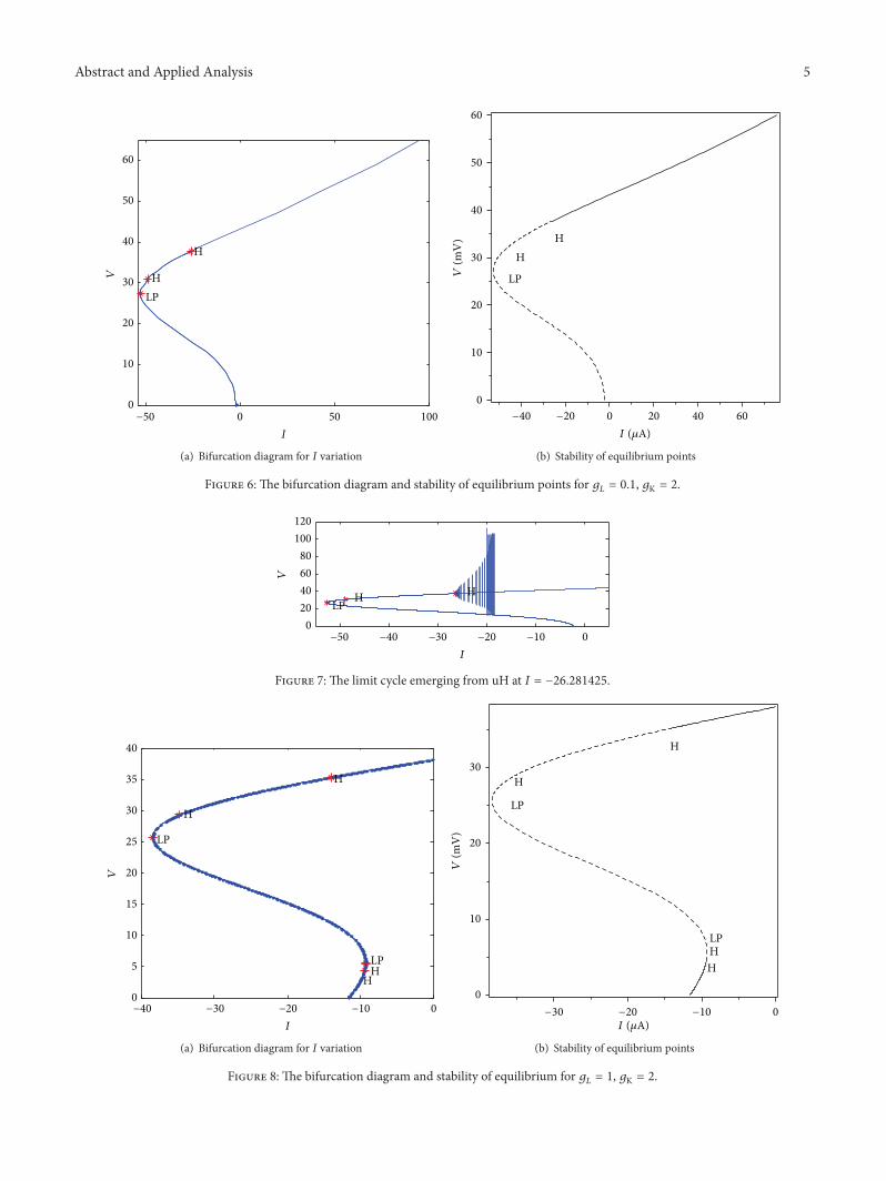
Figure 6: The bifurcation diagram and stability of equilibrium points for 𝑔𝐿= 0.1, 𝑔K = 2.

−50 −40 −30 −20 −10 00

20406080

100120

LPH H

I

V

Figure 7: The limit cycle emerging from uH at 𝐼 = −26.281425.

00

5

10

15

20

25

30

35

40

−40 −30 −20 −10

HH

LP

LP

H

H

I

V

(a) Bifurcation diagram for 𝐼 variation

H

H

HH

LP

LP

V(m

V)

30

20

10

0

−30 −20 −10 0I (𝜇A)


Figure 8: The bifurcation diagram and stability of equilibrium for 𝑔𝐿= 1, 𝑔K = 2.


−40 −35 −30 −25 −20 −15 −10 −5 0−20

0

20

40

60

80

100

120

LPLP

LP

H H H H

H H

H

I

V


−9.55 −9.5 −9.45 −9.4 −9.35 −9.3 −9.25 −9.22

4

6

8

LP

H

H

I

V


0 20 40 60 80 100 120 140

0

10

20

30

40

−20−20

−10

H

H

I

V

(a) Bifurcation diagram for 𝐼 variation

H

H

V(m

V)

25

20

15

10

5

0

−20 0 20 40 60 80 100 120 140

I (𝜇A)

(b) Stability of equilibrium

Figure 11: The bifurcation diagram and stability of equilibrium point for 𝑔𝐿= 2, 𝑔K = 20.


−20 0 20 40 60 80 100 120 140

0

50

100

H

I

V

Figure 12: The limit cycle emerging from uH at 𝐼 = 7.131765 andsH at 𝐼 = 115.224276.



𝑔𝐿= 0.1

𝑔K = 2

𝑉 = −3.692856

𝑚 = 0.033952

ℎ = 0.716772

𝑛 = 0.262913


𝑉 = −0.754488

𝑚 = 0.048408

ℎ = 0.622236

𝑛 = 0.306181


𝑉 = −1.822633

𝑚 = 0.042603

ℎ = 0.658089

𝑛 = 0.290154


𝑉 = 27.252348

𝑚 = 0.559277

ℎ = 0.039851

𝑛 = 0.702462


𝑉 = 30.900097

𝑚 = 0.648151

ℎ = 0.027784

𝑛 = 0.737363


𝑉 = 37.692334

𝑚 = 0.781785

ℎ = 0.015320

𝑛 = 0.791063

𝐼 = −26.281425 uH

25.688959, 𝑚 = 0.518771, ℎ = 0.046889, 𝑛 = 0.686086,𝐼 = −6.575754. The equilibrium points labelled as LP of thethird and fourth are both limit points, where the former has𝑉 = 11.796299, 𝑚 = 0.188048, ℎ = 0.217790, 𝑛 = 0.503195,𝐼 = −9.438630, and the latter has 𝑉 = 20.373201, 𝑚 =

0.378788, ℎ = 0.083800, 𝑛 = 0.623808, 𝐼 = −12.559365.The equilibrium point labelled as H of the sixth is a Hopfbifurcation point with 𝑉 = 31.816299, 𝑚 = 0.668810, ℎ =

0.025491, 𝑛 = 0.745429, 𝐼 = 20.428518, and first Lyapunovcoefficient is negative, and there are two eigenvalues withRe 𝜆1,2

≈ 0; then at the Hopf bifurcation point, HH is stable,and there is a stable limit cycle, so it is the supercritical Hopf



𝑔𝐿= 1

𝑔K = 2

𝑉 = 4.315751

𝑚 = 0.086823

ℎ = 0.442071

𝑛 = 0.385365

𝐼 = −9.406580 uH

𝑉 = 5.346944

𝑚 = 0.097269

ℎ = 0.406190

𝑛 = 0.401801


𝑉 = 5.583327

𝑚 = 0.099807

ℎ = 0.398116

𝑛 = 0.405572


𝑉 = 25.615559

𝑚 = 0.516847

ℎ = 0.047253

𝑛 = 0.685295


𝑉 = 29.221394

𝑚 = 0.608443

ℎ = 0.032689

𝑛 = 0.721865


𝑉 = 35.263043

𝑚 = 0.739314

ℎ = 0.018740

𝑛 = 0.773422

𝐼 = −13.971904 uH

bifurcation (sH). Equilibrium points between the first H andthe sixth H are unstable.

The limit cycle emerging from sH at 𝐼 = 20.428518 is inFigure 4.

The limit cycle emerging from uH at 𝐼 = −11.231605 is inFigure 5.

In Table 1, the bifurcation points found by the Matcontsoftware are presented for 𝑔

𝐿= 2, 𝑔K = 4.

4.2.2. 𝑔𝐿

= 0.1, 𝑔𝐾

= 2. The bifurcation diagrams andthe stability of equilibrium points are obtained in Figure 6.The limit cycle emerging from uH at 𝐼 = −26.281425 isin Figure 7. The bifurcation points found by the Matcontsoftware are presented in Table 2 for 𝑔

𝐿= 0.1, 𝑔K = 2.

From Table 2, we can find the difference in equilibriumpoint.

4.2.3. 𝑔𝐿= 1, 𝑔

𝐾= 2. The bifurcation diagrams and the

stability of equilibrium points are obtained in Figure 8. Thelimit cycles emerging from uH at 𝐼 = −13.971904 and𝐼 = −9.406580 are given in Figures 9 and 10, respectively.The bifurcation points found by the Matcont software arepresented in Table 3 for 𝑔

𝐿= 1, 𝑔K = 2.

4.2.4. 𝑔𝐿= 2, 𝑔

𝐾= 20. The bifurcation diagrams and the

stability of equilibrium points are obtained in Figure 11. Thelimit cycle emerging from uH at 𝐼 = 7.131765 and sH at




𝑔𝐿= 2

𝑔K = 20

𝑉 = 9.688168

𝑚 = 0.153228

ℎ = 0.271065

𝑛 = 0.470616

𝐼 = 7.131765 uH

𝑉 = 24.842866

𝑚 = 0.496500

ℎ = 0.051294

𝑛 = 0.676858

𝐼 = 115.224276 sH

𝐼 = 115.224276 is given in Figure 12. They both are the same.The bifurcation points found by the Matcont software arepresented in Table 4 for 𝑔

𝐿= 2, 𝑔K = 20.

5. Conclusion

In this paper we present the equilibrium point bifurcationand singularity analysis of HH model with constraints. Weinvestigate the effect of constraints and parameters on thetype of equilibrium point bifurcation. We find that if werestrict 𝑉 > 0, then there are new transition sets, and newbifurcation type constrating to the nonconstraint case. TheMatcont toolbox software environment was used for analysisof the bifurcation points in conjunction withMatlab. We givefour different parameters of 𝑔

𝐿, 𝑔K. In each case, we give

equilibrium point bifurcation and also illustrate the stabilityof the equilibriumpoints.This study increases our knowledgeof HH model.

Conflict of Interests

The authors declare that there is no conflict of interestsregarding the publication of this paper.

Acknowledgments

This study is supported by the National Science Foundationof China (Grant no. 11172198) and theNational Basic ResearchProgram of China (Grant no. 11372211).

References

[1] A. L. Hodgkin and A. F. Huxley, “A quantitative descriptionof membrane current and its application to conduction andexcitation in nerve.,” The Journal of Physiology, vol. 117, no. 4,pp. 500–544, 1952.

[2] R. Fitzhugh, “Mathematical models of excitation and prop-agation in nerve,” in Biological Engineer, H. P. Schwan, Ed.,McGraw-Hill, New York, NY, USA, 1969.

[3] J. Cronin, Mathematical Aspects of Hodgkin-HUXley NeuralTheory, Cambridge University Press, 1987.

[4] T. R. L. Chay and J. Keizer, “Minimal model for membraneoscillations in the pancreatic𝛽-cell,”Biophysical Journal, vol. 42,no. 2, pp. 181–189, 1983.

[5] J. Keener and J. Sneyd, Mathematical Physiology, vol. 8 ofInterdisciplinary Applied Mathematics, Springer, New York, NY,USA, 1998.

[6] J. Guckenheimer andP.Holmes,NonlinearOscillations,Dynam-ical Systems, and Bifurcation of Vector Fields, Springer, NewYork, NY, USA, 1983.

[7] J. Guckenheimer and J. S. Labouriau, “Bifurcation of theHodgkin and Huxley equations: a new twist,” Bulletin ofMathematical Biology, vol. 55, no. 5, pp. 937–952, 1993.

[8] Y. A. Bedrov, G. N. Akoev, and O. E. Dick, “Partition of theHodgkin-Huxley type model parameter space into the regionsof qualitatively different solutions,” Biological Cybernetics, vol.66, no. 5, pp. 413–418, 1992.

[9] Y. A. Bedrov, O. E. Dick, A. D. Nozdrachev, and G. N.Akoev, “Method for constructing the boundary of the burstingoscillations region in the neuron model,” Biological Cybernetics,vol. 82, no. 6, pp. 493–497, 2000.

[10] H. Fukai, S. Doi, T. Nomura, and S. Sato, “Hopf bifurcationsin multiple-parameter space of the Hodgkin-Huxley equationsI. Global organization of bistable periodic solutions,” BiologicalCybernetics, vol. 82, no. 3, pp. 215–222, 2000.

[11] H. Fukai, T. Nomura, S. Doi, and S. Sato, “Hopf bifurcations inmultiple-parameter space of the Hodgkin-Huxley equations II.Singularity theoretic approach and highly degenerate bifurca-tions,” Biological Cybernetics, vol. 82, no. 3, pp. 223–229, 2000.

[12] M. Golubitsky and D. G. Schaeffer, Singularities and Groupsin Bifurcation Theory. Vol. I, vol. 51 of Applied MathematicalSciences, Springer, New York, NY, USA, 1985.

[13] Z. Q. Wu and Y. S. Chen, “Classification of bifurcationsfor nonlinear dynamical problems with constraints,” AppliedMathematics and Mechanics, vol. 23, no. 5, pp. 535–541, 2002.

Submit your manuscripts athttp://www.hindawi.com

Hindawi Publishing Corporationhttp://www.hindawi.com Volume 2014

MathematicsJournal of


Mathematical Problems in Engineering

Hindawi Publishing Corporationhttp://www.hindawi.com

Differential EquationsInternational Journal of

Volume 2014

Applied MathematicsJournal of


Probability and StatisticsHindawi Publishing Corporationhttp://www.hindawi.com Volume 2014

Journal of


Mathematical PhysicsAdvances in

Complex AnalysisJournal of


OptimizationJournal of


CombinatoricsHindawi Publishing Corporationhttp://www.hindawi.com Volume 2014

International Journal of


Operations ResearchAdvances in

Journal of


Function Spaces

Abstract and Applied AnalysisHindawi Publishing Corporationhttp://www.hindawi.com Volume 2014

International Journal of Mathematics and Mathematical Sciences


The Scientific World JournalHindawi Publishing Corporation http://www.hindawi.com Volume 2014


Algebra

Discrete Dynamics in Nature and Society



Decision SciencesAdvances in

Discrete MathematicsJournal of

Hindawi Publishing Corporationhttp://www.hindawi.com

Volume 2014 Hindawi Publishing Corporationhttp://www.hindawi.com Volume 2014

Stochastic AnalysisInternational Journal of

Research Article Equilibrium Point Bifurcation and...

Documents

Transcript of Research Article Equilibrium Point Bifurcation and...