Research Article Approximate Analytic Solutions of...
13
Research Article Approximate Analytic Solutions of Transient Nonlinear Heat Conduction with Temperature-Dependent Thermal Diffusivity M. T. Mustafa, 1 A. F. M. Arif, 2 and Khalid Masood 3 1 Department of Mathematics, Statistics and Physics, Qatar University, Doha 2713, Qatar 2 Department of Mechanical Engineering, King Fahd University of Petroleum and Minerals, P.O. Box 5087, Dhahran 31261, Saudi Arabia 3 Department of Mathematics, Hafr Al-Batin Community College, King Fahd University of Petroleum and Minerals, Dhahran 31261, Saudi Arabia Correspondence should be addressed to M. T. Mustafa; [email protected] Received 7 April 2014; Accepted 17 June 2014; Published 13 July 2014 Academic Editor: Mariano Torrisi Copyright © 2014 M. T. Mustafa et al. is is an open access article distributed under the Creative Commons Attribution License, which permits unrestricted use, distribution, and reproduction in any medium, provided the original work is properly cited. A new approach for generating approximate analytic solutions of transient nonlinear heat conduction problems is presented. It is based on an effective combination of Lie symmetry method, homotopy perturbation method, finite element method, and simulation based error reduction techniques. Implementation of the proposed approach is demonstrated by applying it to determine approximate analytic solutions of real life problems consisting of transient nonlinear heat conduction in semi-infinite bars made of stainless steel AISI 304 and mild steel. e results from the approximate analytical solutions and the numerical solution are compared indicating good agreement. 1. Introduction Many physical problems involve transient or unsteady heat conduction. Examples include startup or shutdown of power plant, gas turbine, and heat exchanger. For a homogeneous material with constant properties, the Fourier differential equation =( 2 2 + 2 2 + 2 2 ) (1) with three physical properties or the equation =( 2 2 + 2 2 + 2 2 ) (2) with just one coefficient is solved to predict the temperature distribution during the heating or cooling process. Here is the thermal conductivity, is the density, is the heat capacity, and = / is the thermal diffusivity. ermal diffusivity is a material-specific property for characterizing unsteady heat conduction and it describes how quickly a material reacts to a change in temperature. It should be noted that each of these quantities can vary with temperature. Any change in the thermal boundary conditions around a material results in heat flow in or out of the material until thermal equilibrium is achieved. Materials with a high thermal diffusivity will achieve thermal equilibrium faster than those with lower thermal diffusivity. Most metallic materials have thermal properties (thermal conductivity, specific heat, and density) that are usually temperature-dependent. is results in nonlinearities in the governing partial differential equations (PDEs) describing the temperature distribution through these materials. e analysis of nonlinear heat conduction problems is of increas- ing importance and interest in various engineering and scientific fields. However, no general theory exists for solving nonlinear partial differential equations, and because of the difficulties associated with the solution of nonlinear heat transfer problems, simplifying assumptions are usually made to linearize such problems. For example, constant thermal conductivity is generally assumed for materials having ther- mal conductivity which varies slightly with temperature. However, if temperature change is substantial or the thermal conductivity varies greatly with temperature, the assumption Hindawi Publishing Corporation Abstract and Applied Analysis Volume 2014, Article ID 423421, 12 pages http://dx.doi.org/10.1155/2014/423421
Transcript of Research Article Approximate Analytic Solutions of...

Research ArticleApproximate Analytic Solutions of Transient Nonlinear HeatConduction with Temperature-Dependent Thermal Diffusivity
M T Mustafa1 A F M Arif2 and Khalid Masood3
1 Department of Mathematics Statistics and Physics Qatar University Doha 2713 Qatar2 Department of Mechanical Engineering King Fahd University of Petroleum and Minerals PO Box 5087Dhahran 31261 Saudi Arabia
3 Department of Mathematics Hafr Al-Batin Community College King Fahd University of Petroleum and MineralsDhahran 31261 Saudi Arabia
Correspondence should be addressed to M T Mustafa tahirmustafaqueduqa
Received 7 April 2014 Accepted 17 June 2014 Published 13 July 2014
Academic Editor Mariano Torrisi
Copyright copy 2014 M T Mustafa et al This is an open access article distributed under the Creative Commons Attribution Licensewhich permits unrestricted use distribution and reproduction in any medium provided the original work is properly cited
A new approach for generating approximate analytic solutions of transient nonlinear heat conduction problems is presentedIt is based on an effective combination of Lie symmetry method homotopy perturbation method finite element method andsimulation based error reduction techniques Implementation of the proposed approach is demonstrated by applying it to determineapproximate analytic solutions of real life problems consisting of transient nonlinear heat conduction in semi-infinite bars madeof stainless steel AISI 304 and mild steel The results from the approximate analytical solutions and the numerical solution arecompared indicating good agreement
1 Introduction
Many physical problems involve transient or unsteady heatconduction Examples include startup or shutdown of powerplant gas turbine and heat exchanger For a homogeneousmaterial with constant properties the Fourier differentialequation
120588119888119901
120597119879
120597119905= 119896(
1205972119879
1205971199092+1205972119879
1205971199102+1205972119879
1205971199112) (1)
with three physical properties or the equation
120597119879
120597119905= 120572(
1205972119879
1205971199092+1205972119879
1205971199102+1205972119879
1205971199112) (2)
with just one coefficient is solved to predict the temperaturedistribution during the heating or cooling process Here 119896is the thermal conductivity 120588 is the density 119888119901 is the heatcapacity and 120572 = 119896120588119888119901 is the thermal diffusivity Thermaldiffusivity 120572 is a material-specific property for characterizingunsteady heat conduction and it describes how quickly amaterial reacts to a change in temperature It should be
noted that each of these quantities can vary with temperatureAny change in the thermal boundary conditions arounda material results in heat flow in or out of the materialuntil thermal equilibrium is achieved Materials with a highthermal diffusivity will achieve thermal equilibrium fasterthan those with lower thermal diffusivity
Most metallic materials have thermal properties (thermalconductivity specific heat and density) that are usuallytemperature-dependent This results in nonlinearities in thegoverning partial differential equations (PDEs) describingthe temperature distribution through these materials Theanalysis of nonlinear heat conduction problems is of increas-ing importance and interest in various engineering andscientific fields However no general theory exists for solvingnonlinear partial differential equations and because of thedifficulties associated with the solution of nonlinear heattransfer problems simplifying assumptions are usually madeto linearize such problems For example constant thermalconductivity is generally assumed for materials having ther-mal conductivity which varies slightly with temperatureHowever if temperature change is substantial or the thermalconductivity varies greatly with temperature the assumption
Hindawi Publishing CorporationAbstract and Applied AnalysisVolume 2014 Article ID 423421 12 pageshttpdxdoiorg1011552014423421
2 Abstract and Applied Analysis
of constant thermal conductivitymay lead to significant errorin the solution Therefore such situations require solvingnonlinear transient heat transfer problems It is usually dif-ficult and mathematically challenging to obtain exact closedform solutions of such nonlinear transient heat transferproblems Therefore a number of numerical methods suchas time integration the finite-difference method (FDM) thefinite-element method (FEM) and the boundary-elementmethod (BEM) have been proposed to solve such problems[1ndash5] Though the solutions obtained through sophisticatednumerical techniques are extremely accurate approximationof the analytic solution yet the natural tabular form ofnumerical solutions hampers their real-time applicabilityunlike solutions in functional form An alternate is to lookfor approximate solutions in function form which are moreor less as accurate as numerical solutions Such approximateanalytic solutions can be used in real time and can be easilymanipulated at different points in space and time which mayresult in better insight into physical phenomenon governedby the PDE With this motivation the main objective ofthis work is to implement a new systematic procedure forgenerating approximate solutions of nonlinear heat conduc-tion PDEs in function form which also meet the accuracybenchmarks of numerical solutions As test cases we developmathematical models for heat conduction in stainless steelAISI 304 and mild steel and apply our procedure to findaccurate enough approximate analytic solutions to PDEsgoverning these real-life problems
While there is no general theory for directly solving non-linear PDEs the approach of investigating nonlinear PDEs bytransforming to ODEs or simpler PDEs has worked well insufficient generality compare [6] This includes linearizationtransformations methods of reduction of PDEs to ODEs ortransformations that result in reduction of the complexity ingeneral A powerful general technique for analyzing nonlin-ear PDEs by reducing them to ODEs is given by classical Liesymmetry method also known as similarity method PDEsthat model physical phenomena naturally inherit symmetriesfrom the underlying physical system The similarity methodtakes advantage of these natural symmetries in a PDE andleads to determining special variables namely similarityvariables that give rise to the similarity reduction to ODEsA large amount of literature about the classical Lie symmetrytheory and its applications is available for example [6ndash10]
The purpose of this paper is to apply a new approachfor finding accurate enough approximate analytic solutionsof nonlinear PDEs particularly arising from heat conductionproblems The method utilizes an effective combinationof Lie symmetry analysis homotopy perturbation methodfinite element method and error reduction techniques Asummary of our approach is as follows Lie symmetries arefirst utilized to reduce the initial-boundary value problemof PDE to a boundary value problem of ODE The reducedODE problem is then simultaneously solved by finite elementmethod and homotopy perturbation method to respectivelygenerate numerical solution and initial approximation of theapproximate analytic solution Next using the numericallygenerated solution curve as the benchmark for accuracy anerror reduction of the initial approximation curve is carried
out to generate explicit approximate solution of the ODEproblem Finally the similarity transformation provides theapproximate analytic solution of the IBVP of original PDE
It should be noted that in general the solutions of PDEsare surfaces or hypersurfaces while the solutions of ODEsare represented by curves Furthermore it is well knownthat approximating a surface is an increasingly complex andintractable problem The idea presented here for generatingapproximate solutions of PDE that is approximating the sur-face solution practically involves only approximating a curvewhich is a tractable problem in comparison to the question ofapproximating surfaces This makes it a promising approachespecially when a reasonably accurate initial approximationof the solution curve of ODE can be obtained
In the next section we develop mathematical models forheat conduction in stainless steel AISI 304 and mild steelSection 3 presents the systematic procedure for generatingapproximate analytic solutions using a combination of Liesymmetry finite element homotopy perturbation and errorreduction methods Sections 4 and 5 are devoted to appli-cation of the method for investigation of heat conductionmodels for stainless steel AISI 304 andmild steel respectively
It is assumed that the reader is familiar with standardcomputations of Lie symmetry and homotopy perturbationmethod The reader is referred to [7ndash9 11ndash13] respectivelyfor an introduction to Lie symmetry method and homotopyperturbation method
2 Formulation of Test Problems
Thenonlinear PDE that describes the transient nonlinear heatconduction in a one-dimensional medium is
120597119879 (119909 119905)
120597119905=
120597
120597119909(120572 (119879)
120597119879 (119909 119905)
120597119909) (3)
where 119879(119909 119905) denotes the temperature at a point 119909 at time 119905and 120572(119879) is the temperature-dependent thermal diffusivity ofthe material
To apply our method we will consider test problems forheat conduction in stainless steel AISI 304 andmild steel Forthis purpose the corresponding thermal diffusivity functions120572(119879) need to be modeled first Tables 1 and 2 respectivelygive temperature-dependent thermal properties of AISI 394stainless steel and mild steel considered in this work Trendlines fitted on these datasets show that linear equation is thebest fit for stainless steel as shown in Figure 1 and second-order polynomial is the most accurate fit for mild steel asillustrated in Figure 2 Table 3 gives the estimated thermaldiffusivity functions for stainless steel and mild steel alongwith the goodness of fit (1198772) Using these thermal diffusivityfunctions we will apply our method to investigate transientheat conduction in semi-infinite solid Precisely in Sections 4and 5 approximate analytic solutions will be constructed forinitial-boundary value problem of the form
120597119879 (119909 119905)
120597119905=
120597
120597119909(120572 (119879)
120597119879 (119909 119905)
120597119909)
119879|119905=0 = 119879119894 119879|119909=0 = 119879119904 119879|119909=infin = 119879119894
(4)
Abstract and Applied Analysis 3
0
1
2
3
4
5
6
7
8
9
0
times10minus3
500 1000 1500 2000 2500 3000
Ther
mal
diff
usiv
ity (m
2s
)
Thermal diffusivityLinear (thermal diffusivity)
y = 2E minus 06x + 00037
R2 = 09846
Temperature (K)
Figure 1 Thermal diffusivity of stainless steel AISI 304
0 200 400 600 800 1000 1200
Ther
mal
diff
usiv
ity (m
2s
)
Thermal diffusivityLinear (thermal diffusivity)Poly (thermal diffusivity)
0
5
10
15
20
25
30
times10minus3
y = 1E minus 08x2 minus 3E minus 05x + 00276
R2 = 09956
y = minus2E minus 05x + 00253
R2 = 09776
Temperature (K)
Figure 2 Thermal diffusivity of mild steel
with the thermal diffusivity functions of stainless steel andmild steel respectively
3 The Method for Generating ApproximateAnalytic Solutions
Themain approach for finding approximate analytic solutionsconsists of implementing the steps highlighted below
Given an IBVP of a PDE of the form
119865 (119909 119905 119879 (119909 119905) 119879119909 119879119905 119879119909119909 119879119909119905 119879119905119905) = 0 (5)
Step 1 Reduction of IVBP of PDE to a BVP of ODE theLie symmetries of PDE (5) can be found by employing the
standard well-known procedure compare [7ndash9] It is furtherrequired to systematically identify the symmetry that leavesthe boundaries and boundary conditions invariant [14] Thisis done by taking the most general symmetry operator 119883 ofPDE (5) and finding the conditions under which it leaves theboundaries invariant as well as imposing the restrictions on119883 due to invariance of boundary conditions on the boundaryFurther details about these steps are illustrated in Section 4below The similarity variables of the symmetry that leavesthe whole IBVP invariant will lead to the reduction of IBVPof PDE (5) to a BVP of ODE of the form
119866 (119911 119881 (119911) 119881119911 119881119911119911) = 0 (6)
The aim of the remaining steps is to find an approximatesolution 119881Approx(119911) of BVP of ODE (6) in function form andthen use the similarity transformations of the symmetry toobtain approximate solution 119879(119909 119905) of the IBVP of PDE (5)
Step 2 Find numerical solution 119881Num of BVP of ODE (6)and use this as a benchmark for obtaining function form119881Approx(119911) of the approximate solution of BVP of ODE (6)
Step 3 Obtain an initial guess 119881Initial for the approximateanalytic solution 119881Approx(119911) This is a crucial step as it will beused as a basis to generate approximate analytic solution infunction form Here we use homotopy perturbation methodto obtain initial guess 119881Initial but other kinds of approxima-tions like upperlower solutions can also be employed
Step 4 Improve the initial approximation 119881Initial to get theapproximate analytic solution 119881Approx(119911) up to the desiredlevel of accuracy The improvement in the accuracy of initialapproximation 119881Initial depends on reducing the differencebetween 119881Initial and the benchmark numerical solution curve119881Num of BVP of ODE (6) In case of good initial approxi-mation as obtained in the next sections through homotopyperturbation method the simulation based techniques sim-ilar to noise reduction or smoothing techniques of imageprocessing should be sufficient This idea is implementedin two ways in subsequent sections to improve the level ofaccuracy of approximate analytic solutions In Section 4 thesimulations based on perturbing the initial approximation119881Initial are utilized to generate accurate enough approximateanalytic solution 119881Approx(119911) of the BVP of ODE whereas inSection 5 the error curve obtained through the differenceof 119881Initial and 119881Num is treated to generate the approximateanalytic solution 119881Approx(119911) of the BVP of ODE
Step 5 Use the similarity variables in 119881Approx(119911) to get theapproximate analytic solution 119879(119909 119905) of the IBVP of PDE (5)
Step 6 Validate by carrying out a comparative analysis of theapproximate analytic solution 119879(119909 119905) at different times withthe numerical solution the IBVP of PDE at correspondingtimes
In Sections 4 and 5 we illustrate implementation ofthe above procedure and provide simulation results andapproximate analytic solutions for nonlinear heat conductionin stainless steel and mild steel respectively
4 Abstract and Applied Analysis
Table 1 Thermal properties of AISI 304 stainless steel
Temperature[K]
Specific heat(119888)
[kJkgsdotK]
Conductivity(119896)
[WmK]
Density(120588)
[kgm3]
Thermal diffusivity(120572 = 119896120588119888)(m2s)
100 0272 92 7963 425119864 minus 03
300 0477 149 7900 395119864 minus 03
500 0536 182 7822 434119864 minus 03
700 05695 212 7736 481119864 minus 03
900 05965 24 7644 526119864 minus 03
1100 06255 267 7550 565119864 minus 03
1300 0654 2923 7455 600119864 minus 03
1500 0682 317 7362 631119864 minus 03
1700 071 3417 7269 662119864 minus 03
1900 0738 3663 7175 692119864 minus 03
2100 0766 391 7082 721119864 minus 03
2300 0794 4157 6989 749119864 minus 03
2500 0822 4403 6895 777119864 minus 03
4 Approximate Analytic Solution to IBVP forStainless Steel AISI 304
As first test problem we consider transient heat conductionin a semi-infinite solid bar made of AISI 304 stainless steelwhich is initially at temperature 119879119894 = 300∘K and is subjectedto a surface temperature 119879119904 = 900∘K at 119909 = 0 Thetemperature-dependent diffusivity for stainless steel AISI304 as estimated in Section 2 is given by
120572 (119879) = 119886119879 + 119887 where 119886 = 20 times 10minus6 119887 = 00037 (7)
The objective is to determine an approximate analytic expres-sion for the temperature distribution 119879(119909 119905) satisfying thefollowing IBVP
120597119879 (119909 119905)
120597119905=
120597
120597119909((119886119879 (119909 119905) + 119887)
120597119879 (119909 119905)
120597119909) (8)
119879|119905=0 = 119879119894 119879|119909=0 = 119879119904 119879|119909=infin = 119879119894 (9)
where 119886 = 20 times 10minus6 and 119887 = 00037It is first required to systematically find the symmetry
that preserves the IBVP ((8) (9)) Applying the Lie symmetrytheory [7ndash9] the Lie symmetry algebra of the PDE (8) isdetermined to be four-dimensional and is generated by
1198831 =120597
120597119909 1198832 =
120597
120597119905 1198833 = 119909
120597
120597119909+ 2119905
120597
120597119905
1198834 =119886119909
2
120597
120597119909+ (119886119879 + 119887)
120597
120597119879
(10)
In order to obtain the symmetry that leaves the whole IBVPinvariant we consider the general symmetry operator
119883 = 11989611198831 + 11989621198832 + 11989631198833 + 11989641198834 (11)
of PDE (8) and search for the operator that preserves theboundary and the boundary conditions (9)
The invariance of the boundaries 119909 = 0 119905 = 0 orequivalently
[119883 (119909 minus 0)]119909=0 = 0
[119883 (119905 minus 0)]119905=0 = 0
(12)
implies
1198961 = 1198962 = 0 (13)
so119883must be
119883 = 11989631198833 + 11989641198834 (14)
In addition to the restrictions imposed by (13) the invarianceof initial and boundary conditions that is
[119883 (119879 minus 119879119894)]119905=0 = 0 on 119879 = 119879119894
[119883 (119879 minus 119879119904)]119909=0 = 0 on 119879 = 119879119904
(15)
implies that we must have
1198964 = 0 (16)
Hence the IBVP (8) (9) is invariant under the symmetry
119883 = 119909120597
120597119909+ 2119905
120597
120597119905 (17)
where we have chosen 1198963 = 1 The similarity variables
119911 (119909 119905) =119909
radic119905 119881 (119911) = 119879 (18)
of 119883 imply that the solution of IBVP (8) (9) is of the form119879 = 119881(119911) where 119881(119911) satisfies the ODE
(119886119881 + 119887)1198892119881
1198891199112+ 119886(
119889119881
119889119911)
2
+119911
2
119889119881
119889119911= 0 (19)
Abstract and Applied Analysis 5
Table 2 Thermal properties of mild steel
Temperature[K]
Specific heat(119888)
[kJkgsdotK]
Conductivity(119896)
[WmK]
Density(120588)
[kgm3]
Thermal diffusivity(120572 = 119896120588119888)(m2s)
100 0346 681 7892 249119864 minus 02
1458 03662 6636 7883 230119864 minus 02
1917 03863 6462 7874 212119864 minus 02
2375 04065 6288 7866 197119864 minus 02
2833 04267 6113 7857 182119864 minus 02
3292 04468 5939 7848 169119864 minus 02
375 0467 5765 7840 157119864 minus 02
4208 04864 5579 7827 147119864 minus 02
4667 0505 538 7809 136119864 minus 02
5125 05236 5181 7791 127119864 minus 02
5583 05421 4981 7772 118119864 minus 02
6042 05616 4782 7753 110119864 minus 02
650 05905 458 7726 100119864 minus 02
800 0685 392 7726 741119864 minus 03
1000 1169 30 7726 332119864 minus 03
with the boundary conditions
119881 (119911 = 0) = 119879119904 = 900 119881 (119911 = infin) = 119879119894 = 300 (20)
Next the reduced BVP (19) (20) is to be simultaneouslysolvednumerically andby employing homotopy perturbationmethod The homotopy solution will be utilized later asinitial guess for the approximate analytic solution of BVP(19) (20) whereas numerical solution will be used as thebenchmark curve to improve the accuracy of the initiallyguessed homotopy solution
In order to apply homotopy perturbation method [11ndash13]for finding approximate closed form solution of the boundaryvalue problem (19) (20) we construct a homotopy of theexpression (19) in the following form
1198871198892119881
1198891199112+119911
2
119889119881
119889119911+ 119901(119886119881
1198892119881
1198891199112+ 119886(
119889119881
119889119911)
2
) = 0 (21)
The homotopy parameter 119901 has values 0 or 1 the value 119901 = 0corresponds to a linear equation which can easily be solvedand the value 119901 = 1 corresponds to the original equation (19)The solution119881(119911) can be expanded in terms of the homotopyparameter 119901 as follows
119881 = 1198810 + 1199011198811 + 11990121198812 + sdot sdot sdot (22)
Substituting (22) in (21) and equating coefficients of the samepowers of 119901 we obtain a set of equations from which the firsttwo consist of the equation
11988711988921198810
1198891199112+119911
2
1198891198810
119889119911= 0 (23)
with the boundary conditions
1198810 (119911 = 0) = 119879119904 1198810 (119911 997888rarr infin) = 119879119894 (24)
and the equation
11988711988921198811
1198891199112+119911
2
1198891198811
119889119911+ 1198861198810
11988921198810
1198891199112+ 119886(
1198891198810
119889119911)
2
= 0 (25)
with the boundary conditions
1198811 (0) = 0 1198811 (119911 997888rarr infin) = 0 (26)
The solution of the boundary value problem (23) (24) caneasily be obtained as
1198810 (119911) = 119879119904 minus (119879119904 minus 119879119894) erf (119911
2radic119887) (27)
Substituting solution (27) in (25) and removing the secularterms we obtain
11988711988921198811
1198891199112+119911
2
1198891198811
119889119911+119886119890minus11991122119887(119879119904 minus 119879119894)
2
119887120587
+ 119911119886119890minus11991122119887
(119879119904 minus 119879119894) 119879119904
23radic119887radic120587
= 0
(28)
The solution of the boundary value problem (28) and (26) canbe written in the following form
1198811 (119911)
=119886 (119879119904 minus 119879119894)
2119887
times 1199113radic1198872119890minus11991122119887119879119904
radic120587
+ (1 minus erf ( 119911
2radic119887)) erf ( 119911
2radic119887) (119879119904 minus 119879119894)
(29)
6 Abstract and Applied Analysis
300
400
500
600
700
800
900
0 500 1000 1500 2000
z
VNumVInitial
Figure 3 Initial approximation 119881Initial and numerical solution 119881Numof BVP (19) (20)
Since we are looking for an approximate closed form solutionof the problem (19) setting 119901 = 1 in (22) we obtain a firstorder approximate solution
119881 (119911) = 1198810 (119911) + 1198811 (119911) (30)
Substituting (27) and (29) in (30) we obtain an approximateclosed form solution of BVP (19) (20) in the following form
119881 (119911) = 119879119904 minus (119879119904 minus 119879119894) erf (119911
2radic119887)
+119886 (119879119904 minus 119879119894)
2119887
times 1199113radic1198872119890minus11991122119887119879119904
radic120587
+(1 minus erf ( 119911
2radic119887)) erf ( 119911
2radic119887) (119879119904 minus 119879119894)
(31)
We call this solution the initial guess 119881Initial for the intendedapproximate analytic solution of the BVP (19) (20)
The numerical solution119881Num of BVP (19) (20) is obtainedusing finite elementmethodDefining the initial relative erroras
119864Initial =119881Initial minus 119881Num
119881Num (32)
it is found that
Max 1003816100381610038161003816119864Initial1003816100381610038161003816 = 006119845971 (33)
Figure 3 gives the plots of the initial approximation119881Initial andthe numerical solution 119881Num while the initial relative error119864Initial is shown in Figure 5
In order to improve the accuracy level of the initialapproximation (31) we introduce the parameters 120572 120573 120575 120598and 120582 in (31) to obtain the expression
(119911) = 119879119904 minus (119879119904 minus 119879119894) erf (120598119911
2radic119887) +
119886 (119879119904 minus 119879119894)
2119887
times 1205731199113radic1198872119890minus(120572119911)
22119887119879119904
radic120587
+(1 minus erf ( 120575119911
2radic119887)) erf ( 120582119911
2radic119887) (119879119904 minus 119879119894)
(34)
Small variations of the parameters from the values
120572 = 1 120573 = 1 120575 = 1 120598 = 1 120582 = 1 (35)
in (119911) generate a sequence of curves in the neighborhoodof the initial approximation curve 119881initial Several carefulnumerical simulations are performed for small variation ofthe above parameters leading to the values
120572 = 14 120573 = 1 120575 = 093
120598 = 09101 120582 = 091
(36)
for which the relative error between (119911) and 119881Num is lessthan 04
Hence we obtain an approximate analytic solution119881Approxof BVP (19) (20) as
119881Approx (119911)
= 119879119904 minus (119879119904 minus 119879119894) erf (120598119911
2radic119887) +
119886 (119879119904 minus 119879119894)
2119887
times 1205731199113radic1198872119890minus(120572119911)
22119887119879119904
radic120587
+(1 minus erf ( 120575119911
2radic119887)) erf ( 120582119911
2radic119887) (119879119904 minus 119879119894)
(37)
where the parameters 120572 120573 120575 120598 and 120582 are given by (36) with
Max100381610038161003816100381610038161003816100381610038161003816
119881Approx minus 119881Num
119881Num
100381610038161003816100381610038161003816100381610038161003816
= 0003959810186 (38)
Theplots of the numerical solution119881Num and the approximateanalytic solution 119881Approx are given in Figure 4 and Figure 5shows the plot of Error(119911) where
Error (119911) =119881Approx minus 119881Num
119881Num (39)
Abstract and Applied Analysis 7
Table 3 Thermal diffusivity functions considered in the current study
Material Thermal diffusivity function120572(119879) m2s 119877
2 Temperature range(K)
Stainless steelAISI 304
120572(119879) = 119886119879 + 119887
119886 = 20 times 10minus6 119887 = 00037
09968 100ndash2500
Mild steel120572(119879) = 119886119879
2+ 119887119879 + 119888
119886 = 10 times 10minus8 119887 = minus30 times 10
minus5119888 = 00276
09957 100ndash1000
300
400
500
600
700
800
900
0 500 1000 1500 2000
z
VNumVApprox
Figure 4 Approximate analytic solution 119881Approx and numericalsolution 119881Num of BVP (19) (20)
minus008
minus006
minus004
minus002
0
002
004
006
008
0 500 1000 1500 2000
z
EInitialError(z)
Figure 5Comparison of relative errors for the initial approximationand approximate analytic solution of BVP (19) (20)
Finally the similarity variables (18) provide the approxi-mate analytic solution of IBVP (8) (9) as
119879 (119909 119905) = 119879119904 minus (119879119904 minus 119879119894) erf (120598 (119909radic119905)
2radic119887) +
119886 (119879119904 minus 119879119894)
2119887
times
120573(119909radic119905)3radic1198872119890minus(120572(119909radic119905))
2
2119887119879119904
radic120587
900
800
700
600
500
400
300
0500
10001500
2000 510
1520
25
xt
Figure 6 Approximate analytic solution119879(119909 119905) of the IBVP (8) (9)
+ (1 minus erf (120575 (119909radic119905)
2radic119887))
times erf (120582 (119909radic119905)
2radic119887) (119879119904 minus 119879119894)
(40)
where the parameters 120572 120573 120575 120598 and 120582 are given by (36) Asurface plot of the approximate analytic solution 119879(119909 119905) isprovided in Figure 6
For validation purpose we carry out a comparativeanalysis of the approximate analytic solution 119879(119909 119905) and thenumerical solution of IBVP (8) (9) In order to numericallysolve the IBVP (8) (9) a transient thermal analysis isperformed using FEA software ANSYS The given structureis modeled using 3D Conduction Bar Elements (LINK33)LINK33 is a uniaxial element with the ability to conduct heatbetween its nodes The element has a single degree of free-dom temperature at each node point The conducting baris applicable to a steady-state or transient thermal analysis Arefined uniformmesh is used tomodel the nonlinear thermalgradient through the solid The length of the model is takenas 119871 = 2m assuming that no significant temperature changeoccurs at the interior end point during the time period of
8 Abstract and Applied Analysis
300
400
500
600
700
800
900
0 500 1000 1500 2000
Tem
pera
ture
x
Numerical solution at t = 5
Numerical solution at t = 10
Numerical solution at t = 15
Numerical solution at t = 25
Approximate solution at t = 5
Approximate solution at t = 10
Approximate solution at t = 15
Approximate solution at t = 25
Figure 7 Comparison of approximate analytic solution 119879(119909 119905) andnumerical solution of IBVP (8) (9) at different times
interest This assumption is validated by the temperature ofnode at 119909 = 119871 at the end of the transient analysis
Figure 7 shows the comparison of temperature distribu-tion at different times using the approximate analytic solution(40) and the numerical solutions at corresponding timesThefigure shows good agreement between approximate analyticsolution and the numerical results
5 Approximate Analytic Solution toIBVP for Mild Steel
In this test problem we consider transient heat conductionin a semi-infinite solid bar made of mild steel which isinitially at temperature 119879119894 = 300∘K and is subjected to asurface temperature 119879119904 = 900∘K at 119909 = 0 The temperature-dependent diffusivity for mild steel as estimated in Section 2is given by
120572 (119879) = 1198861198792+ 119887119879 + 119888
where 119886 = 10 times 10minus8 119887 = minus30 times 10minus5 119888 = 00276
(41)
The objective is to determine an approximate analytic expres-sion for the temperature distribution 119879(119909 119905) satisfying thefollowing IBVP
120597119879 (119909 119905)
120597119905=
120597
120597119909((119886119879(119909 119905)
2+ 119887119879 (119909 119905) + 119888)
120597119879 (119909 119905)
120597119909)
(42)
119879|119905=0 = 119879119894 119879|119909=0 = 119879119904 119879|119909=infin = 119879119894 (43)
where 119886 = 10 times 10minus8 119887 = minus30 times 10minus5 and 119887 = 00276In order to identify the symmetry that preserves the IBVP
(42) (43) we first find the Lie symmetry algebra of the PDE
(42) which is determined to be three-dimensional and isgenerated by
1198831 =120597
120597119909 1198832 =
120597
120597119905 1198833 = 119909
120597
120597119909+ 2119905
120597
120597119905 (44)
Using the restrictions imposed by the boundaries and bound-ary conditions in themanner similar to Section 4 we find thatthe symmetry that leaves the whole IBVP (42) (43) invariantis
119883 = 119909120597
120597119909+ 2119905
120597
120597119905 (45)
The similarity variables
119911 (119909 119905) =119909
radic119905 119881 (119911) = 119879 (46)
of 119883 imply that the solution of IBVP (42) (43) is of the form119879 = 119881(119911) where 119881(119911) satisfies the ODE
(1198861198812+ 119887119881 + 119888)
1198892119881
1198891199112+ (2119886119881 + 119887) (
119889119881
119889119911)
2
+119911
2
119889119881
119889119911= 0
(47)
with the boundary conditions
119881 (119911 = 0) = 119879119904 = 900 119881 (119911 = infin) = 119879119894 = 300 (48)
Next the reduced BVP (47) (48) is simultaneously solvednumerically and by homotopy perturbation method Thehomotopy solution will be utilized below as initial guess119881Initial for the approximate analytic solution 119881Approx of BVP(47) (48) whereas the numerical solution 119881Num will beused as the benchmark curve to improve the accuracy ofthe initially guessed homotopy solution In order to findhomotopy solution 119881Initial of the boundary value problem(47) (48) we construct a homotopy of the expression (47)in the following form
1198881198892119881
1198891199112+119911
2
119889119881
119889119911
+ 119901[1198861198812 1198892119881
1198891199112+ 119887119881
1198892119881
1198891199112+ 2119886119881(
119889119881
119889119911)
2
+ 119887(119889119881
119889119911)
2
] = 0
(49)
Abstract and Applied Analysis 9
VNumVInitial
300
400
500
600
700
800
900
0 500 1000 1500 2000
z
Figure 8 Initial approximation 119881Initial and numerical solution 119881Numof BVP (47) (48)
and apply the same procedure as in the previous section toobtain an approximate closed form solution of the BVP (47)(48) as
119881 (119911) = 119879119904 minus (119879119904 minus 119879119894) erf (119911
2radic119888) +
119890minus11991122119888(119879119904 minus 119879119894)
12119888120587
times minus 6119887119879119904 + 11989011991122119888 erf 119888 ( 119911
2radic119888)
times (41198861205871198792
119904minus 4119886120587119879
2
119904erf 119888( 119911
2radic119888)
2
minus 6119887120587119879119894 erf (119911
2radic119888) + 6119887119879119904
+ 9119887120587119879119904 erf (119911
2radic119888) minus 4119886120587119879119904119879119894
+ 4119886120587119879119904119879119894 erf 119888(119911
2radic119888)
2
)
(50)
We call this solution the initial guess 119881Initial for the intendedapproximate analytic solution of the BVP (47) (48)
Thenumerical solution119881Num of BVP (47) (48) is obtainedusing finite elementmethodDefining the initial relative erroras
119864Initial =119881Initial minus 119881Num
119881Num (51)
it is found that
Max 1003816100381610038161003816119864Initial1003816100381610038161003816 = 01500655840 (52)
Figure 8 gives the plots of the initial approximation119881Initial andthe numerical solution 119881Num while the initial relative error119864Initial is shown in Figure 11
0
10
20
30
40
50
60
70
80
0 500 1000 1500 2000
z
Δ = VInitial minus VNum
Figure 9 The difference Δ between the initial approximation 119881Initialand numerical solution 119881Num of BVP (47) (48)
In order to improve the accuracy level of the initialapproximation (31) we adopt an approach different from theprevious section and focus on approximating the differencebetween 119881Num and 119881Initial in function form Plotting thedifference
Δ (119911) = 119881Initial minus 119881Num (53)
as shown in Figure 9 implies that the difference Δ(119911) canbe represented by a skewed function As an ansatz forapproximating Δ(119911) we take the skewed function of the form
119891 (119911) = 120573119890minus1198701199112
erf (120572119911) (54)
where the parameter 120572 mainly contributes to the location ofthe peak the parameter 119870 mainly affects the shrinking orexpanding of the skewed curve and 120573 controls the height ofthe peak of the curve Performing several careful numericalsimulations suggest the values of the parameters
120572 = 00105 119870 = 0000014 120573 = 10102 (55)
giving accurate enough function form representation of Δ(119911)that makes the relative error between approximate analyticsolution and numerical solution about 07 as shown below
Defining
119881Approx (119911) = 119881Initial minus 120573119890minus1198701199112
erf (120572119911) (56)
where the parameters 120572 120573 and 119870 are given by (55) providesan approximate analytic solution 119881Approx of BVP (47) (48)with
Max100381610038161003816100381610038161003816100381610038161003816
119881Approx minus 119881Num
119881Num
100381610038161003816100381610038161003816100381610038161003816
= 000740878478 (57)
Theplots of the numerical solution119881Num and the approximateanalytic solution 119881Approx are given in Figure 10 and Figure 11shows the plot of Error(119911) where
Error (119911) =119881Approx minus 119881Num
119881Num (58)
10 Abstract and Applied Analysis
300
400
500
600
700
800
900
0 500 1000 1500 2000
z
VNumVApprox
Figure 10 Approximate analytic solution 119881Approx and numericalsolution 119881Num of BVP (47) (48)
0 500 1000 1500 2000
z
EInitial
0
002
004
006
008
01
012
014
016
Error(z)
Figure 11 Comparison of relative errors for the initial approxima-tion and approximate analytic solution of BVP (47) (48)
Finally the similarity variables (46) provide the approxi-mate analytic solution of IBVP (42) (43) as
119879 (119909 119905) = 119879119904 minus (119879119904 minus 119879119894) erf (119909radic119905
2radic119888) +
119890minus(119909radic119905)
2
2119888(119879119904 minus 119879119894)
12119888120587
times minus 6119887119879119904 + 11989011991122119888 erf 119888 (119909
radic119905
2radic119888)
times (41198861205871198792
119904minus 4119886120587119879
2
119904erf 119888(119909
radic119905
2radic119888)
2
minus 6119887120587119879119894 erf (119909radic119905
2radic119888) + 6119887119879119904
900
800
700
600
500
400
300
0500
10001500
2000x 5
1015
2025
t
Figure 12 Approximate analytic solution 119879(119909 119905) of the IBVP (42)and (43)
+ 9119887120587119879119904 erf (119909radic119905
2radic119888) minus 4119886120587119879119904119879119894
+ 4119886120587119879119904119879119894 erf 119888(119909radic119905
2radic119888)
2
)
minus 120573119890minus1198701199112
erf (120572119911) (59)
where the parameters 120572 120573 and119870 are given by (55) A surfaceplot of the approximate analytic solution 119879(119909 119905) is providedin Figure 12
For validation purpose we carry out a comparativeanalysis of the approximate analytic solution 119879(119909 119905) andthe numerical solution of IBVP (42) (43) The numericalsolutions of IBVP (42) (43) are obtained by performing atransient thermal analysis using FEA software ANSYS asexplained in the previous section Figure 13 shows the com-parison of temperature distribution at different times usingthe approximate analytic solution (59) and the numericalsolutions at corresponding times The figure shows goodagreement between approximate analytic solution and thenumerical results
6 Conclusion
Themathematical modeling of most of the physical processesin fields like diffusion chemical kinetics fluid mechanicswave mechanics and general transport problems is governedby such nonlinear PDEs whose exact analytic solutions arehard to find Therefore the methods of finding approximateanalytic solutions become important in investigating suchnonlinear PDEs In this paper we present a new systematicprocedure for generating approximate analytic solutions ofnonlinear PDEs particularly arising from heat conduc-tion problems The methodology followed here exploits an
Abstract and Applied Analysis 11
300
400
500
600
700
800
900
Tem
pera
ture
0 500 1000 1500 2000
x
Numerical solution at t = 5
Numerical solution at t = 10
Numerical solution at t = 15
Numerical solution at t = 25
Approximate solution at t = 5
Approximate solution at t = 10
Approximate solution at t = 15
Approximate solution at t = 25
Figure 13 Comparison of approximate analytic solution119879(119909 119905) andnumerical solution of IBVP (42) and (43) at different times
effective combination of Lie symmetry analysis homotopyperturbation method finite element method and simulationbased error reduction techniques The similarity variables ofan appropriate Lie symmetry are first utilized to reduce theIBVP of PDE to a BVP of ODE The reduced ODE problemis then simultaneously solved numerically and by homotopyperturbation method to respectively generate numericalsolution and initial approximation of the approximate ana-lytic solution of BVP of ODE Next using the numericallygenerated solution curve as the accuracy benchmark anerror reduction of the initial approximation is carried outby utilizing simulations to generate an approximate analyticsolution which meets the accuracy benchmark of numericalsolution Finally the similarity transformations provide theapproximate analytic solution of the IBVP of the origi-nal PDE The approach is applied to obtain approximateanalytic solutions for test problems consisting of transientheat conduction in bars made of stainless steel AISI 304and mild steel The validity of solutions is verified by acomparison between the approximate analytic solutions andthe numerical solutions of the test problems The resultsindicate good agreement between the approximate analyticalsolutions and the corresponding numerical solutions Theidea presented here to get approximate analytic solutionof PDE that is approximating the surface 119879(119909 119905) prac-tically involves approximating a curve 119881(119911) which is atractable problem in comparison to increasingly complexand intractable problem of approximating the surface 119879(119909 119905)itself It can become particularly efficient when a reasonablyaccurate initial approximation of the solution curve 119881(119911) ofthe reduced ODE can be obtained as was the case here inthe form of homotopy solutions Another advantage of theapproximate analytic solutions obtained by our approach isthat these can be used in real time or negligible CPU time to
evaluate the solution of the PDE with the same accuracy asthe numerical solution
Although here we have restricted applications of ourapproach to heat conduction problems it can be adapted forobtaining approximate analytic solutions for the class of PDEswhere the PDE can be reduced to an ODE through similarityvariables For instance the approach can be directly appliedto all the reduced-via-similarity BVPs of ODEs in [15] Forfurther application the approach can be extended to obtainapproximate solutions where the reduction is a system ofODEs like the reduced laminar boundary layer problems in[16 17]
Conflict of Interests
The authors declare that there is no conflict of interestsregarding the publication of this paper
References
[1] K W Morton and D F Mayers Numerical Solution of PartialDifferential Equations An Introduction Cambridge UniversityPress New York NY USA 1994
[2] J Blobner R A Białecki and G Kuhn ldquoBoundary-elementsolution of coupled heat conduction-radiation problems inthe presence of shadow zonesrdquo Numerical Heat Transfer BFundamentals vol 39 no 5 pp 451ndash478 2001
[3] B Chen Y Gu Z Guan and H Zhang ldquoNonlinear transientheat conduction analysis with precise time integrationmethodrdquoNumerical Heat Transfer B vol 40 no 4 pp 325ndash341 2001
[4] F Asllanaj A Milandri G Jeandel and J R Roche ldquoAfinite difference solution of non-linear systems of radiative-conductive heat transfer equationsrdquo International Journal forNumericalMethods in Engineering vol 54 no 11 pp 1649ndash16682002
[5] A Fic R A Białecki and A J Kassab ldquoSolving transientnonlinear heat conduction problems by proper orthogonaldecomposition and the finite-elementmethodrdquoNumerical HeatTransfer B Fundamentals vol 48 no 2 pp 103ndash124 2005
[6] W FAmesNonlinear Partial Differential Equations in Engineer-ing vol 1 Academic Press New York NY USA 1965
[7] G W Bluman and S Anco Symmetry and Integration Methodsfor Differential Equations Springer New York NY USA 2002
[8] N H Ibragimov Elementary Lie Group Analysis and OrdinaryDifferential Equations vol 4 John Wiley amp Sons ChichesterUK 1999
[9] P J Olver Applications of Lie Groups to Differential EquationsSpringer New York NY USA 1986
[10] L V Ovsiannikov Group Analysis of Differential EquationsAcademic Press New York NY USA 1982
[11] J H He ldquoHomotopy perturbation techniquerdquo Computer Meth-ods in Applied Mechanics and Engineering vol 178 no 3-4 pp257ndash262 1999
[12] J He ldquoBookkeeping parameter in perturbation methodsrdquoInternational Journal of Nonlinear Sciences and Numerical Sim-ulation vol 2 no 3 pp 257ndash264 2001
[13] J-H He ldquoAddendum new interpretation of homotopy pertur-bation methodrdquo International Journal of Modern Physics B vol20 no 18 pp 2561ndash2568 2006
12 Abstract and Applied Analysis
[14] H Azad M T Mustafa and A F M Arif ldquoAnalytic solutions ofinitial-boundary-value problems of transient conduction usingsymmetriesrdquo Applied Mathematics and Computation vol 215no 12 pp 4132ndash4140 2010
[15] L Dresner Similarity Solutions of Nonlinear Partial DifferentialEquations vol 88 of Research Notes in Mathematics SeriesLongman 1983
[16] A Aziz ldquoA similarity solution for laminar thermal boundarylayer over a flat plate with a convective surface boundary con-ditionrdquo Communications in Nonlinear Science and NumericalSimulation vol 14 no 4 pp 1064ndash1068 2009
[17] S Mukhopadhyay K Bhattacharyya and G C Layek ldquoSteadyboundary layer flow and heat transfer over a porous movingplate in presence of thermal radiationrdquo International Journal ofHeat and Mass Transfer vol 54 no 13-14 pp 2751ndash2757 2011
Submit your manuscripts athttpwwwhindawicom
Hindawi Publishing Corporationhttpwwwhindawicom Volume 2014
MathematicsJournal of
Hindawi Publishing Corporationhttpwwwhindawicom Volume 2014
Mathematical Problems in Engineering
Hindawi Publishing Corporationhttpwwwhindawicom
Differential EquationsInternational Journal of
Volume 2014
Applied MathematicsJournal of
Hindawi Publishing Corporationhttpwwwhindawicom Volume 2014
Probability and StatisticsHindawi Publishing Corporationhttpwwwhindawicom Volume 2014
Journal of
Hindawi Publishing Corporationhttpwwwhindawicom Volume 2014
Mathematical PhysicsAdvances in
Complex AnalysisJournal of
Hindawi Publishing Corporationhttpwwwhindawicom Volume 2014
OptimizationJournal of
Hindawi Publishing Corporationhttpwwwhindawicom Volume 2014
CombinatoricsHindawi Publishing Corporationhttpwwwhindawicom Volume 2014
International Journal of
Hindawi Publishing Corporationhttpwwwhindawicom Volume 2014
Operations ResearchAdvances in
Journal of
Hindawi Publishing Corporationhttpwwwhindawicom Volume 2014
Function Spaces
Abstract and Applied AnalysisHindawi Publishing Corporationhttpwwwhindawicom Volume 2014
International Journal of Mathematics and Mathematical Sciences
Hindawi Publishing Corporationhttpwwwhindawicom Volume 2014
The Scientific World JournalHindawi Publishing Corporation httpwwwhindawicom Volume 2014
Hindawi Publishing Corporationhttpwwwhindawicom Volume 2014
Algebra
Discrete Dynamics in Nature and Society
Hindawi Publishing Corporationhttpwwwhindawicom Volume 2014
Hindawi Publishing Corporationhttpwwwhindawicom Volume 2014
Decision SciencesAdvances in
Discrete MathematicsJournal of
Hindawi Publishing Corporationhttpwwwhindawicom
Volume 2014 Hindawi Publishing Corporationhttpwwwhindawicom Volume 2014
Stochastic AnalysisInternational Journal of
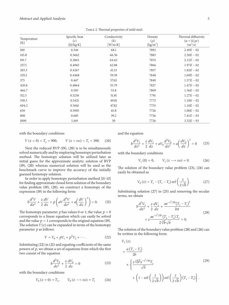
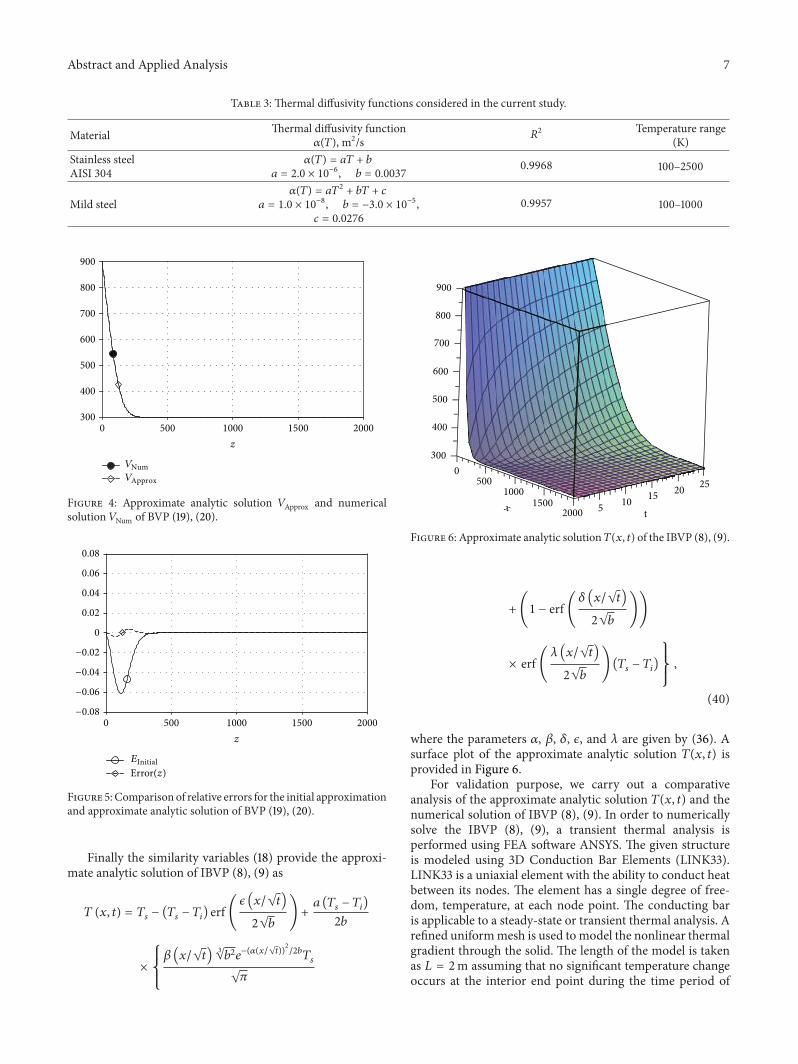