REPORT DOCUMENTATION PAGE Form Approved · Appendix I. BobCAD-CAM Job Creation..... 41 Introduction...

The public reporting burden for this collection of information is estimated to average 1 hour per response, including the time for reviewing instructions,

searching existing data sources, gathering and maintaining the data needed, and completing and reviewing the collection of information. Send comments

regarding this burden estimate or any other aspect of this collection of information, including suggesstions for reducing this burden, to Washington

Headquarters Services, Directorate for Information Operations and Reports, 1215 Jefferson Davis Highway, Suite 1204, Arlington VA, 22202-4302.

Respondents should be aware that notwithstanding any other provision of law, no person shall be subject to any oenalty for failing to comply with a collection of

information if it does not display a currently valid OMB control number.

PLEASE DO NOT RETURN YOUR FORM TO THE ABOVE ADDRESS.

a. REPORT

Bull’s-Eye Structure with a Sub-Wavelength Circular Aperture

14. ABSTRACT

16. SECURITY CLASSIFICATION OF:

This research focuses on improving the spatial resolution of terahertz (THz) imaging. Using a sub-wavelength

aperture in a metal ground plane is the most common way to improve the spatial resolution, but a sub-wavelength

aperture has low radiation transmission. To increase the radiation transmission of a sub-wavelength aperture,

periodic circular grooves were put in the metal around the aperture. The sub-wavelength circular aperture and the

periodic circular grooves around it are known as the bull’s-eye structure. The bull’s-eye structure shows high

1. REPORT DATE (DD-MM-YYYY)

4. TITLE AND SUBTITLE

30-08-2013

13. SUPPLEMENTARY NOTES

The views, opinions and/or findings contained in this report are those of the author(s) and should not contrued as an official Department

of the Army position, policy or decision, unless so designated by other documentation.

12. DISTRIBUTION AVAILIBILITY STATEMENT

Approved for public release; distribution is unlimited.

UU

9. SPONSORING/MONITORING AGENCY NAME(S) AND

ADDRESS(ES)

6. AUTHORS

7. PERFORMING ORGANIZATION NAMES AND ADDRESSES

U.S. Army Research Office

P.O. Box 12211

Research Triangle Park, NC 27709-2211

15. SUBJECT TERMS

Terahertz (THz) imaging, sub-wavelength aperture, bull’s-eye structure, periodic circular grooves, spatial resolution, radiation

transmission, High Frequency Structure Simulator (HFSS), CAD

Masoud Zarepoor

University of California - Irvine

5171 California Avenue, Suite 150

Irvine, CA 92697 -7600

REPORT DOCUMENTATION PAGE

b. ABSTRACT

UU

c. THIS PAGE

UU

2. REPORT TYPE

MS Thesis

17. LIMITATION OF

ABSTRACT

UU

15. NUMBER

OF PAGES

5d. PROJECT NUMBER

5e. TASK NUMBER

5f. WORK UNIT NUMBER

5c. PROGRAM ELEMENT NUMBER

5b. GRANT NUMBER

5a. CONTRACT NUMBER

W911NF-11-1-0024

611103

Form Approved OMB NO. 0704-0188

58162-EL-MUR.47

11. SPONSOR/MONITOR'S REPORT

NUMBER(S)

10. SPONSOR/MONITOR'S ACRONYM(S)

ARO

8. PERFORMING ORGANIZATION REPORT

NUMBER

19a. NAME OF RESPONSIBLE PERSON

19b. TELEPHONE NUMBER

Peter Burke

949-824-9326

3. DATES COVERED (From - To)

Standard Form 298 (Rev 8/98)

Prescribed by ANSI Std. Z39.18

-


Report Title

ABSTRACT

This research focuses on improving the spatial resolution of terahertz (THz) imaging. Using a sub-wavelength

aperture in a metal ground plane is the most common way to improve the spatial resolution, but a sub-wavelength

aperture has low radiation transmission. To increase the radiation transmission of a sub-wavelength aperture, periodic

circular grooves were put in the metal around the aperture. The sub-wavelength circular aperture and the periodic

circular grooves around it are known as the bull’s-eye structure. The bull’s-eye structure shows high radiation

transmission at its design frequency, and it also has sub-wavelength spatial resolution. This research designed the

bull’s-eye structure to perform at ~3 mm wavelength in W band (75-110 GHz). Simulations were conducted on the

3D model of the bull’s-eye structure to study its performance in the desired frequency range. Then a bull’s-eye

structure was fabricated and tested by the knife-edge technique to measure its spatial resolution. The knife-edge test

results show the obtained sub-wavelength spatial resolution of the fabricated bull’s-eye structure. This research also

includes the designs of a 500 GHz bull’s-eye structure and 100 GHz reflective probe.


A thesis submitted in partial fulfillment

Of the requirements for the degree of

Master of Science in Engineering

By

Masoud Zarepoor

B.S., Shiraz University, 2010

2013

Wright State University

WRIGHT STATE UNIVERSITY

GRADUATE SCHOOL

May 30, 2013 I HEREBY RECOMMEND THAT THE THESIS PREPARED UNDER MY SUPERVISION BY Masoud Zarepoor ENTITLED Bull’s-Eye Structure with a Sub-Wavelength Circular Aperture BE ACCEPTED IN PARTIAL FULFILLMENT OF THE REQUIREMENTS FOR THE DEGREE OF Master of Science in Engineering.

______________________________

Joseph C. Slater, Ph.D., P.E Thesis Director

_________________________________ George Huang, Ph.D.

Chair, Department of Mechanical and Materials

Engineering College of Engineering and Computer Science

Committee on Final Examination

_________________________________

Joseph C. Slater, PhD., P.E

_________________________________

Elliott R. Brown, PhD.

_________________________________ Henry D. Young, PhD.

_________________________________ R. William Ayres, Ph.D. Interim Dean, Graduate School

iii

ABSTRACT

Zarepoor Masoud. M.S. Department of Mechanical and Materials Engineering, Wright State University, 2013. Bull’s-eye Structure with a Sub-Wavelength Circular Aperture.

This research focuses on improving the spatial resolution of terahertz (THz)

imaging. Using a sub-wavelength aperture in a metal ground plane is the most common

way to improve the spatial resolution, but a sub-wavelength aperture has low radiation

transmission. To increase the radiation transmission of a sub-wavelength aperture,

periodic circular grooves were put in the metal around the aperture. The sub-wavelength

circular aperture and the periodic circular grooves around it are known as the bull’s-eye

structure. The bull’s-eye structure shows high radiation transmission at its design

frequency, and it also has sub-wavelength spatial resolution. This research designed the

bull’s-eye structure to perform at ~3 mm wavelength in W band (75-110 GHz).

Simulations were conducted on the 3D model of the bull’s-eye structure to study its

performance in the desired frequency range. Then a bull’s-eye structure was fabricated

and tested by the knife-edge technique to measure its spatial resolution. The knife-edge

test results show the obtained sub-wavelength spatial resolution of the fabricated bull’s-

eye structure. This research also includes the designs of a 500 GHz bull’s-eye structure

and 100 GHz reflective probe.

iv

ACKNOWLEDGEMENT

In the first place, I want to thank Dr. Elliott R. Brown for his great help and support

during my research in the THz sensors group. Also, I thank Dr. Joseph C. Slater for his

guidance and encouragement during my MS studies and my other committee member,

Dr. Henry D. Young.

In addition, I appreciate John Middendorf, Dr. Matthieu Martin, Leamon Viveros, John

Cetnar, and Mads Larsen for their helpful discussion and comments.

Finally, I thank Brandy Foster for her help with English grammar on my written Thesis

document.

v

Table of Content 1. Introduction ..................................................................................................................... 1

1.1 Background ............................................................................................................... 1

1.2 Overview ................................................................................................................... 4

2. Design of the Bull’s-Eye Structure with a Sub-Wavelength Circular Aperture ............. 6

2.1 Design and Dimensions of the Bull’s-Eye Structure ................................................ 6

3. Simulation and Fabrication of the Bull’s-Eye Structure with a Sub-Wavelength

Circular Aperture .............................................................................................................. 11

3.1 Introduction to HFSS .............................................................................................. 11

3.2 HFSS Settings ......................................................................................................... 11

3.2.1 Boundary Condition and Excitation ................................................................. 11

3.3 Simulation Results for the 3-mm-Wavelength Bull’s-Eye Structure ...................... 12

3.3.1 Aperture Diameter Optimization for the 3-mm-Wavelenght Bull’s-Eye

Structure..................................................................................................................... 12

3.3.2 3-mm-Wavelength Bull’s-Eye Structure (1mm Distance from Wave Port) .... 15

3.3.3 3-mm-Wavelength Bull’s-Eye Structure (0.5 mm Distance from Wave Port) 18

3.3.4 3-mm-Wavelength Bull’s-Eye Structure (3 mm Distance from Wave Port) ... 20

3.4 Sub-Wavelength Circular Aperture without Bull’s-Eye Structure (0.5 mm Distance

from Wave Port) ............................................................................................................ 23

3.5 500 GHz Bull’s-Eye Structure ................................................................................ 27

3.6 Fabrication of 3-mm-Wavelength Bull’s-Eye Structure ......................................... 28

4. Experimental Measurement .......................................................................................... 30

4.1 Spatial Resolution Measurement Method ............................................................... 30

vi

4.2 Knife-Edge Test ...................................................................................................... 30

4.3 Results of the Knife-Edge Test: Spatial Resolution Curves ................................... 32

5. Design and Simulation of the 100 GHz Reflective Probe ............................................ 35

5.1 Probe Applications .................................................................................................. 35

5.2 Design and Simulation of the Reflective Probe ...................................................... 36

6. Conclusion .................................................................................................................... 39

Appendix I. BobCAD-CAM Job Creation........................................................................ 41

Introduction ................................................................................................................... 41

Milling ........................................................................................................................... 41

Lathe .............................................................................................................................. 41

Post-Processor ............................................................................................................... 42

Bull’s-Eye Structure Design in BobCAD ..................................................................... 43

Summary & Notes ......................................................................................................... 53

Appendix II. HFSS Meshing and Convergence ................................................................ 55

Mathematical Procedure ................................................................................................ 55

Shape Functions ............................................................................................................ 56

Conformal Meshing....................................................................................................... 57

Adaptive Meshing ......................................................................................................... 58

Convergence Criterion .................................................................................................. 58

REFERENCES ................................................................................................................. 61

vii

List of Figures

Figure 1. The cross section of a bull’s-eye structure showing an aperture in a metal film with 3 periodic grooves around the aperture. ...................................................................... 6

Figure 2. Computed radiation transmission for the (a) bow-tie aperture (b) bow-tie aperture and circular aperture with and without bull’s-eye structure (BE) ....................... 7

Figure 3. Designed bull’s-eye structure with a circular aperture in HFSS. ...................... 12

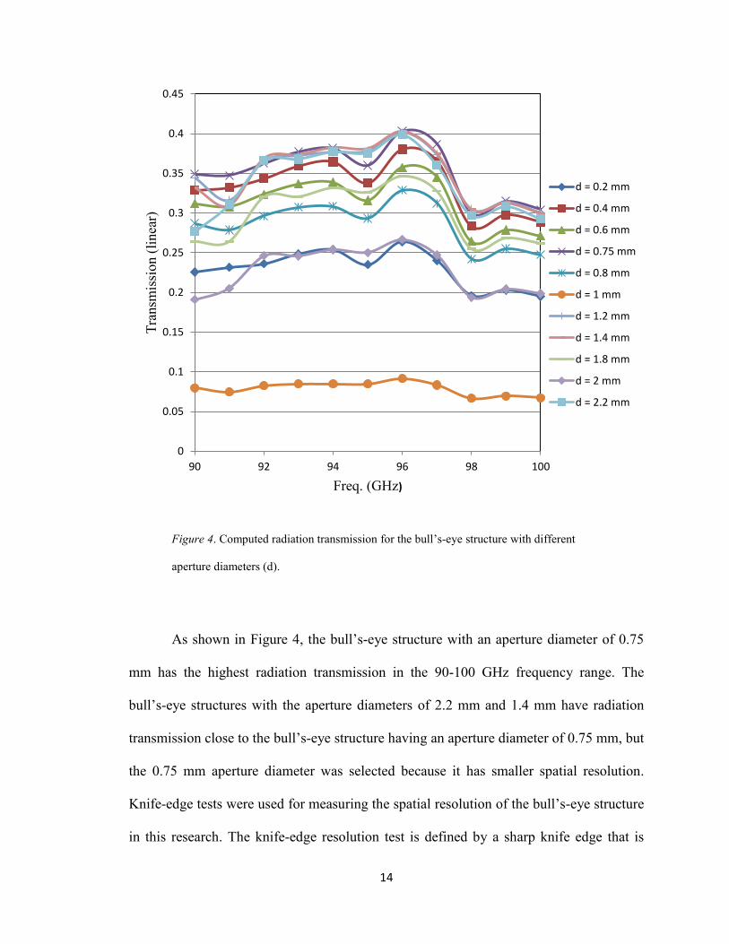
Figure 4. Computed radiation transmission for the bull’s-eye structure with different aperture diameters (d). ...................................................................................................... 14

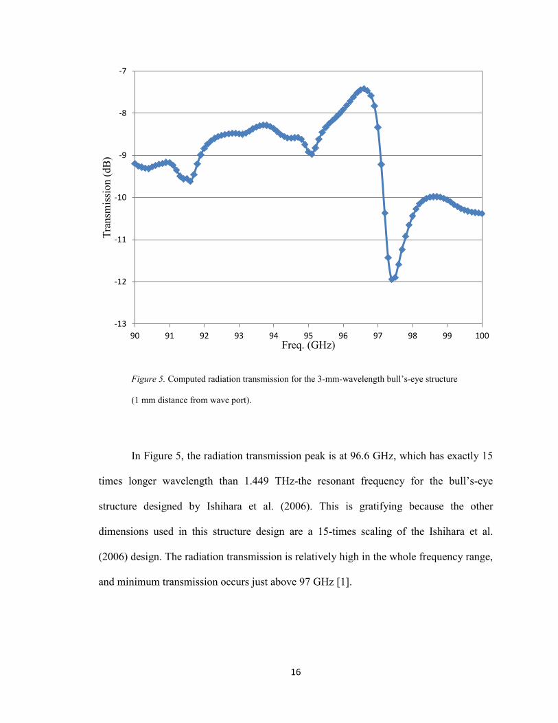
Figure 5. Computed radiation transmission for the 3-mm-wavelength bull’s-eye structure (1 mm distance from wave port). ...................................................................................... 16

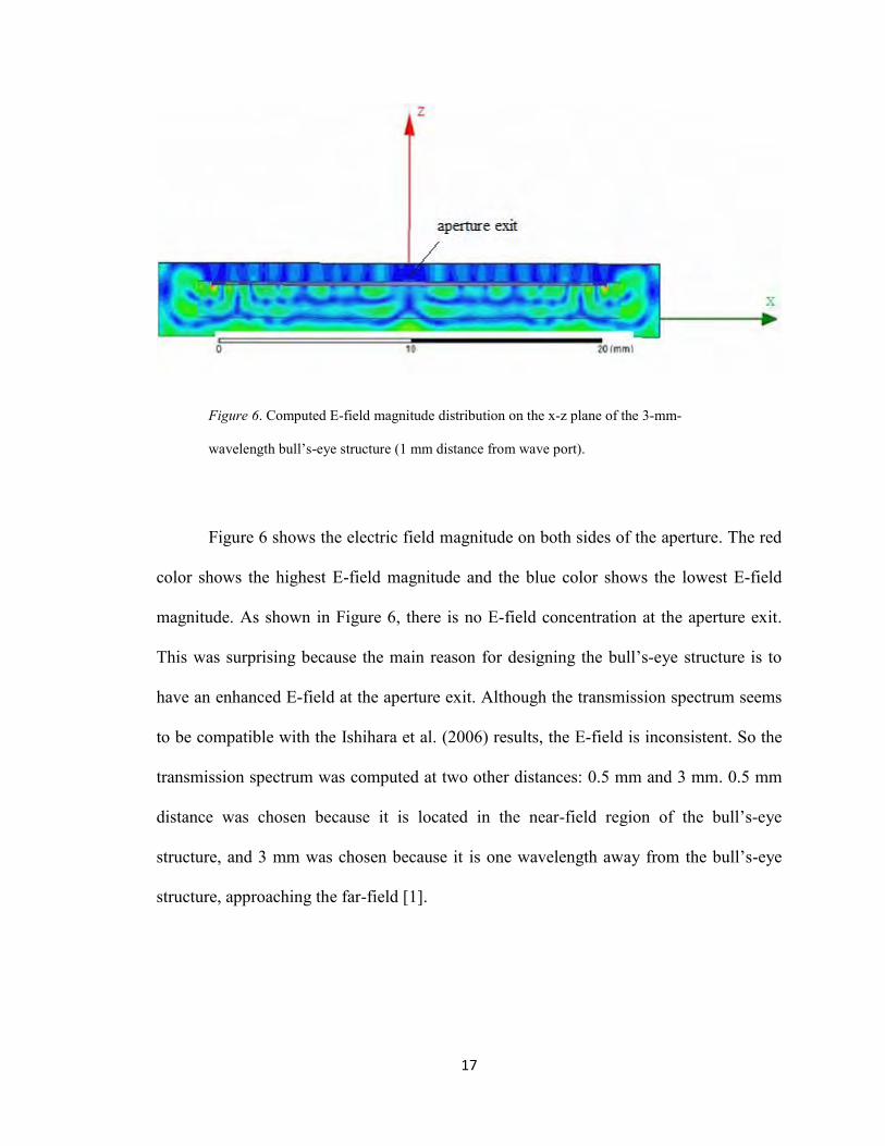
Figure 6. Computed E-field magnitude distribution on the x-z plane of the 3-mm-wavelength bull’s-eye structure (1 mm distance from wave port). .................................. 17

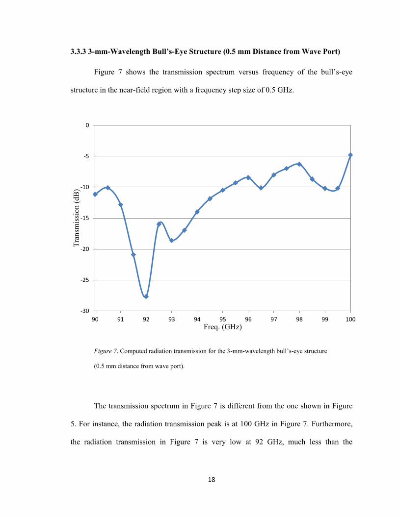
Figure 7. Computed radiation transmission for the 3-mm-wavelength bull’s-eye structure (0.5 mm distance from wave port). ................................................................................... 18

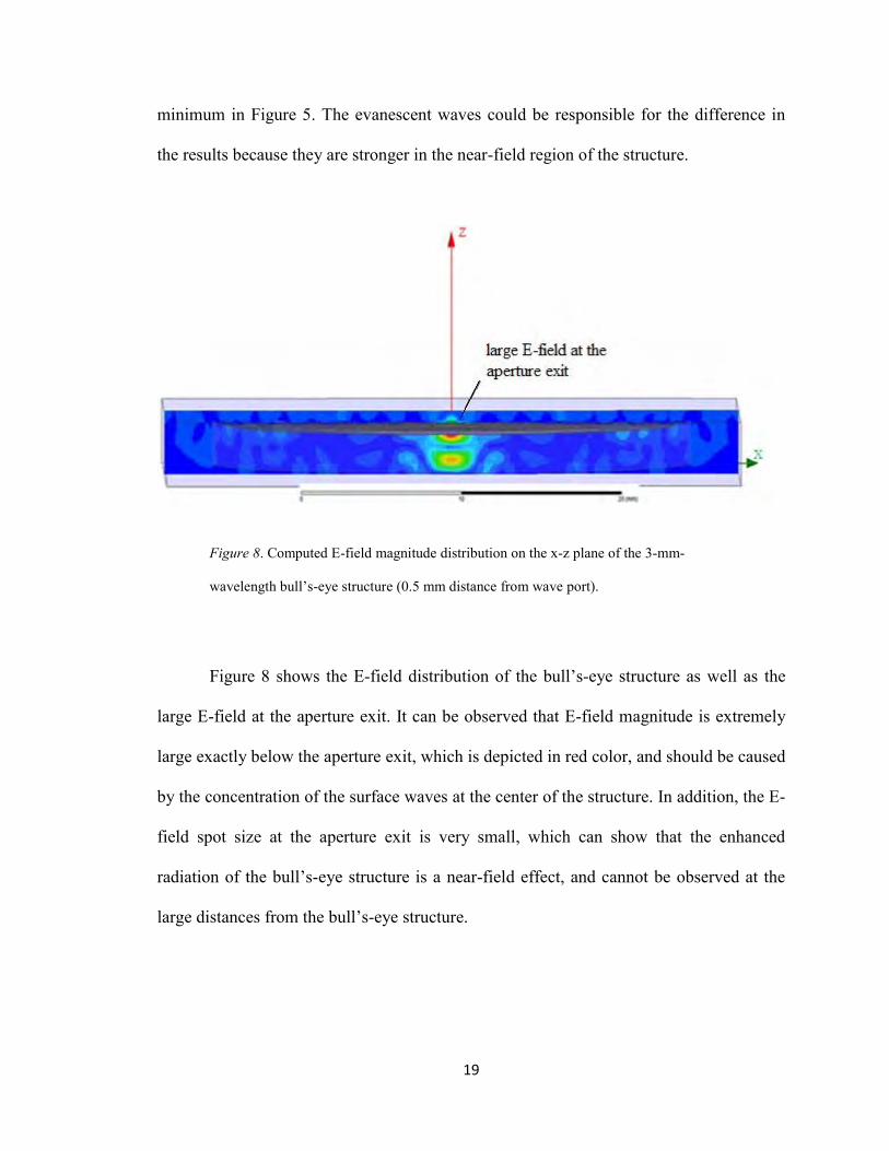
Figure 8. Computed E-field magnitude distribution on the x-z plane of the 3-mm-wavelength bull’s-eye structure (0.5 mm distance from wave port). ............................... 19

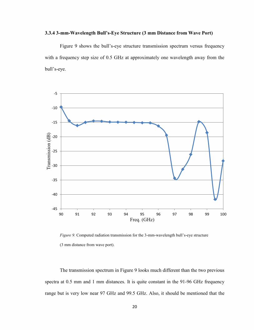
Figure 9. Computed radiation transmission for the 3-mm-wavelength bull’s-eye structure (3 mm distance from wave port). ...................................................................................... 20

Figure 10. Computed E-field magnitude distribution on the x-z plane of the 3-mm-wavelength bull’s-eye structure (3 mm distance from wave port). .................................. 21

Figure 11. Comparison of computed transmission spectra for 3-mm-wavelength bull’s-eye structure at three different distances. .......................................................................... 22

Figure 12. Sub-wavelength circular aperture in the silver film on the Teflon substrate. . 23

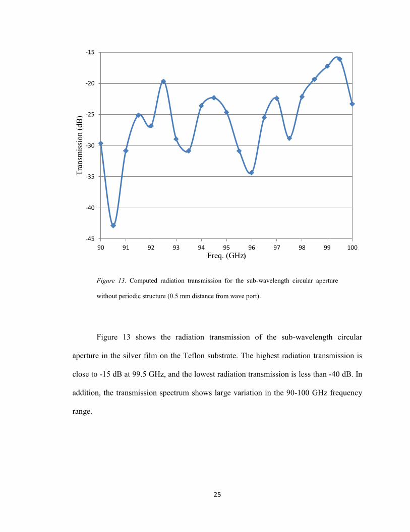
Figure 13. Computed radiation transmission for the sub-wavelength circular aperture without periodic structure (0.5 mm distance from wave port). ......................................... 25

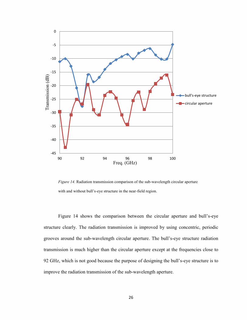
Figure 14. Radiation transmission comparison of the sub-wavelength circular aperture with and without bull’s-eye structure in the near-field region. ......................................... 26

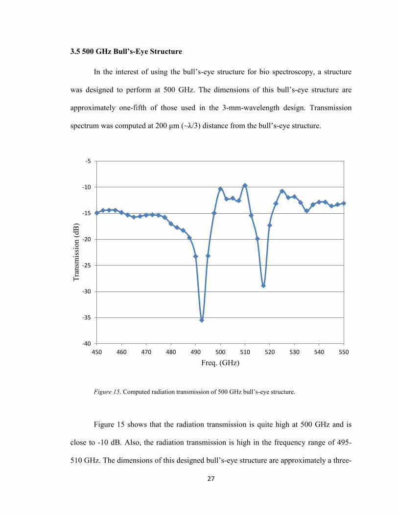
Figure 15. Computed radiation transmission of 500 GHz bull’s-eye structure. ............... 27

Figure 16. Computed E-field magnitude distribution on the x-z plane of the 500 GHz bull’s-eye structure............................................................................................................ 28

viii

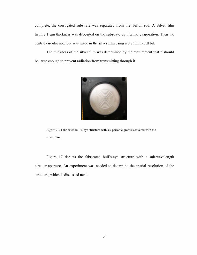
Figure 17. Fabricated bull’s-eye structure with six periodic grooves covered with the silver film. ......................................................................................................................... 29

Figure 18. Knife-edge test set up for measuring the bull’s-eye structure spatial resolution............................................................................................................................................ 31

Figure 19. Measured spatial resolution curve along the X-axis. ...................................... 32

Figure 20. Measured spatial resolution curve along the Y-axis. ...................................... 33

Figure 21. Comparison of interaction volume and spatial resolution of (a) large-tip-sized probe (b) tiny-tip-sized probe [19]. ................................................................................... 35

Figure 22. Designed 100 GHz reflective probe. ............................................................... 36

Figure 23. Reflection spectrum of the designed probe. .................................................... 37

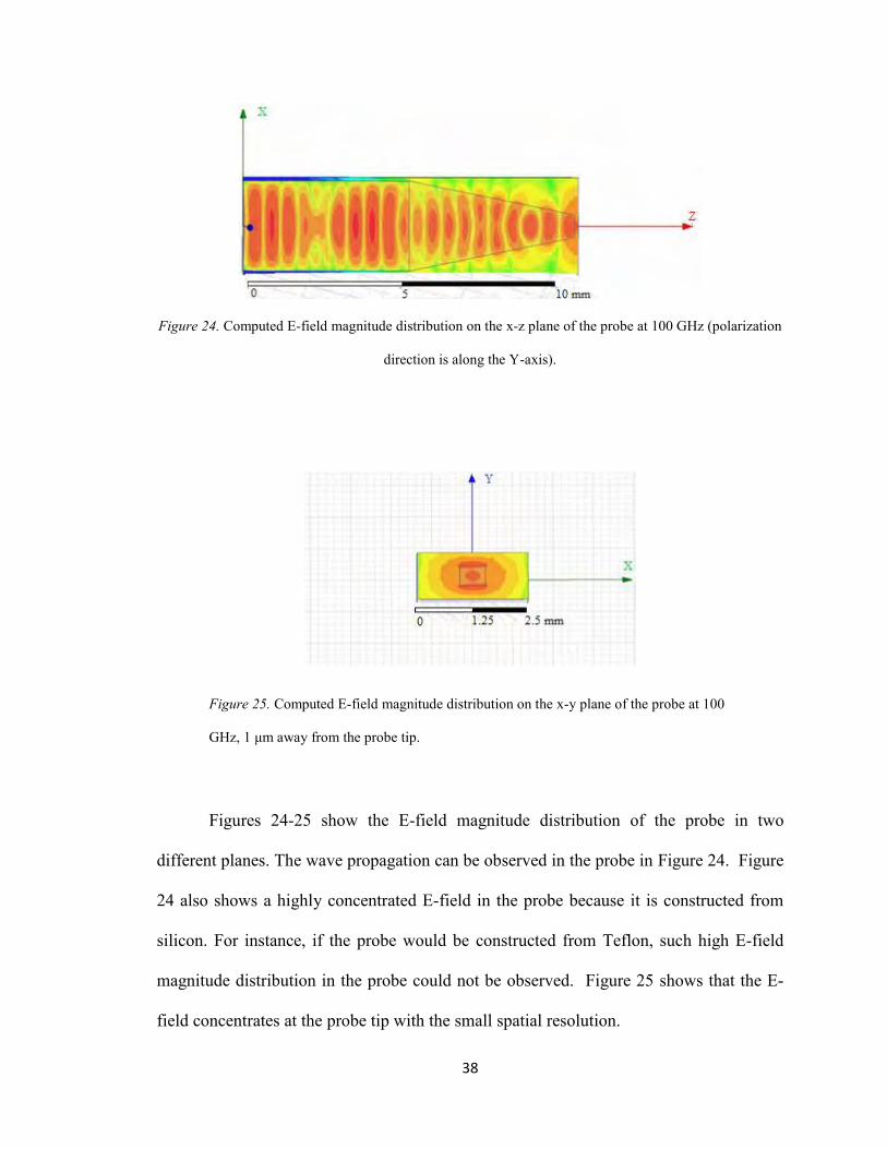
Figure 24. Computed E-field magnitude distribution on the x-z plane of the probe at 100 GHz (polarization direction is along the Y-axis). ............................................................. 38

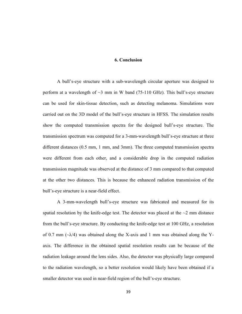
Figure 25. Computed E-field magnitude distribution on the x-y plane of the probe at 100 GHz, 1 μm away from the probe tip. ................................................................................ 38

Figure 26. Setting “Units” and turning on “Lathe Coordinates”. ..................................... 43

Figure 27. Setting the stock values. .................................................................................. 44

Figure 28. Entering the stock values. ............................................................................... 45

Figure 29. Adding the tool path. ....................................................................................... 46

Figure 30. Selecting the geometry. ................................................................................... 47

Figure 31. Setting the “Feature Rough”. .......................................................................... 47

Figure 32. Setting “Rapids”. ............................................................................................. 48

Figure 33. Setting “Leads”. .............................................................................................. 49

Figure 34. Setting the tool parameters. ............................................................................. 50

Figure 35. Setting “Orientation”. ..................................................................................... 51

Figure 36. Setting the tool home position (Home Position Z and Home Position X). ..... 51

Figure 37. Selecting the post-processor............................................................................ 52

Figure 38. Posting the G-code. ......................................................................................... 53

Figure 39. HFSS procedure for finding fields and S matrix............................................. 55

Figure 40. A 3D tetrahedral element. ............................................................................... 56

Figure 41. Conformal system of meshing ........................................................................ 57

Figure 42. A correct convergence profile . ....................................................................... 59

Figure 43. A changing convergence profile . ................................................................... 60

ix

List of Tables

Table 1. Bull’s-eye structure parameters designed by Ishihara et al. (2006) [1]. ............... 8

Table 2. Bull’s-eye structure parameters (designed to perform at ~3 mm wavelength). .... 9

Table 3. Bull’s-eye structure parameters (designed to perform at 500 GHz). .................. 10

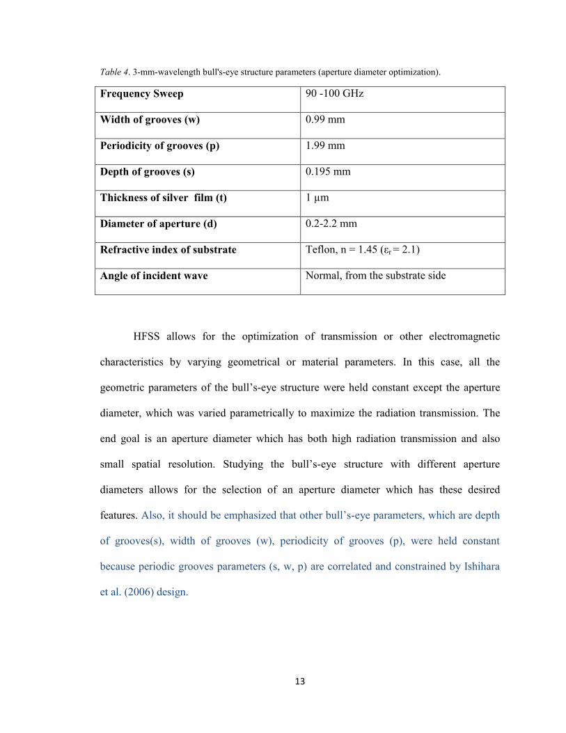
Table 4. 3-mm-wavelength bull's-eye structure parameters (aperture diameter

optimization). .................................................................................................................... 13

Table 5. Sub-wavelength circular aperture without the bull’s-eye structure parameters. 24

1

1. Introduction

1.1 Background

Much research has been conducted in the field of terahertz (THz) imaging due to

the specific properties of THz waves. THz imaging has many applications in biomedical

imaging, nondestructive monitoring, component testing, and quality inspection of

products [2]. The spatial resolution of THz imaging is poor compared to infrared or

visible imaging because the THz region corresponds to the wavelengths between tens of

micrometer to one millimeter, so an improvement in the spatial resolution of the THz

imaging needs to be accomplished. A common way to improve the spatial resolution is to

use a sub-wavelength aperture [1].

Many researchers have studied the radiation transmission of an aperture. Bethe

[3] and Bouwkamp [4] described the theoretical model of radiation going through the

circular sub-wavelength aperture. They described the radiation going through an aperture

in an infinitesimal opaque metallic screen. Also, they explained how the E-field of the

transmitted radiation changes with distance from the aperture [5].

Any metal has a variable penetration depth in different spectral regions.

Therefore, the thickness of a metal film should be much larger than its penetration depth

in order to have negligible radiation transmission through the metal film compared to the

radiation transmitted through a sub-wavelength aperture [5, 6].

2

In addition, many different shapes of apertures have been designed, such as a C-

shaped [7], I-shaped [8], and H-shaped [9]. The main advantage of these alternative

aperture shapes compared to a circular aperture is that they all have small gaps between

their ridges. The E-field magnitude is large in the small gaps between the ridges, so this

large E-field magnitude yields higher radiation transmission compared to a circular

aperture. A sub-wavelength aperture reduces the signal strength. As a result, the main

problem caused by a small aperture is the low radiation transmission. Therefore, the goal

of this research is to enhance the radiation transmission of a small aperture.

Many designs have been proposed and tested in order to enhance the radiation

transmission of a sub-wavelength aperture, and findings have shown that using a

corrugated structure around an aperture should be an effective solution. When the

incident radiation is focused to a spot size much larger than the aperture, it causes the

resonant excitation of the surface waves (in the THz region) or the surface plasmons (in

the optical region). The excitation of surface waves or surface plasmons is caused by the

corrugated structure around the aperture. The corrugated structure around an aperture can

have different shapes. The most common is the concentric, circular, periodic grooves

surrounding a sub-wavelength aperture. This structure is known as a bull’s-eye structure

and can be fabricated on a metal plate or on a dielectric substrate covered with a thin

metal film. Finally, the excited surface waves or surface plasmons concentrate at the

center of the structure, which results in more radiation transmission [1, 5].

In the visible region, Thio et al. (2001) studied the optical radiation transmission

through a sub-wavelength aperture in a metal film surrounded by concentric, periodic

grooves. They observed three times more radiation transmission for this design than the

3

circular aperture without the corrugated surface. Thio et al. (2002) then used the bull’s-

eye structure for near-field scanning applications [10, 11].

Lezec et al. (2002) studied the radiation through a sub-wavelength aperture and

noted that it diffracts with a large angular divergence. By fabricating periodic grooves

around the aperture, they observed that the radiation had a much smaller angular

divergence, and could be controlled in the direction of the radiation [12].

Akarca-Biyikli, Bulu, and Ozbay, (2004) investigated theoretically and

experimentally the microwave radiation transmission through a sub-wavelength aperture

in a corrugated metal plate, and measured the transmission of the fabricated structures in

the 8-30 mm wavelength range. They obtained ~50 % radiation transmission with small

angular divergence radiation for their designed structures [13].

Mahboub et al. (2010) theoretically and experimentally investigated the optimal

geometric parameters of a bull’s-eye structure in the optical region. They found that the

geometric parameters in the bull’s-eye structure are interlinked. To illustrate, they found

the relationship between the design resonant wavelength and periodicity of the grooves,

as well as the relationship between the other geometric parameters with the design

resonant wavelength. Their results indicate the ability to fabricate a bull’s-eye structure

with the optimal radiation transmission at the desired frequency [14].

In the THz region, Ishihara et al. (2005) studied the radiation transmission

through a bull's-eye structure with a sub-wavelength circular aperture. The bull’s-eye

structure was fabricated in a metal plate. Their designed bull’s-eye structure had 20 times

more THz radiation transmission than a circular aperture without periodic structure at the

4

design frequency of 1.5 THz. Also, they reached a sub-wavelength resolution (λ/4) at the

design frequency [5, 15].

Then Ishihara et al. (2006) designed a bull’s-eye structure with a bow-tie aperture.

Instead of using a thick metal plate for their design, they used a corrugated dielectric

substrate covered with a thin metal film. They reached a spatial resolution of 12 µm

(λ/17) in the near-field region [1, 5].

Finally, a bull’s-eye structure can be used for sub-wavelength resolution

transmission imaging around 100 GHz. A small feature (such as skin-cancer tissue)

should be placed in the near-field region of a bull’s-eye aperture on its transmission side

for imaging purposes. Bull’s-eye structures are used for imaging small features because

normal optical components in this frequency region are limited to diffraction-limited

resolution, which is typically several wavelengths. Additionally, these optical

components are not appropriate for detecting features with a sub-wavelength size and

obtained images, having these optical components as transmission devices, do not have

high contrast.

1.2 Overview

The object of this research is to design and fabricate a bull’s-eye structure with a

sub-wavelength circular aperture to perform at a wavelength of ~3 mm in W band (75-

110 GHz). This bull’s-eye structure can be used for skin tissue detection, such as

detecting skin burns and melanoma. The designs of a 500 GHz bull’s-eye structure (with

an application in biological sensing and detection) and a 100 GHz silicon reflective probe

(with an application in identifying melanoma and skin burns) are also carried out. It is

necessary to note that this research is not limited to design and computer simulation of

5

bull’s-eye structures, and it has significant fabrication and experimentation. Bull’s-eye

structures were fabricated with high precision using a CNC lathe machine and a thermal

evaporator. Then, quality of fabricated bull’s-eye structures was evaluated by conducting

thorough experimental measurements with a pretty complex setup.

This Thesis contains six chapters. In the second chapter, the designs of 3-mm-

wavelength and 500 GHz bull’s-eye structures are presented. In the third chapter, the

simulation results for the designed bull’s-eye structures are presented. The simulation

results show the computed transmission spectra for the designed bull’s-eye structures in

the desired frequency ranges. The fabrication process of the 3-mm-wavelength bull’s-eye

structure is also demonstrated in the third chapter. In the fourth chapter, the experimental

results for the fabricated 3-mm-wavelength bull’s-eye structure are presented. The

experimental results show the measured spatial resolution of the fabricated bull’s-eye

structure. The simulation results for the designed 100 GHz reflective probe are reported

in the fifth chapter. The conclusion of the Thesis is presented in the sixth chapter.

6

2. Design of the Bull’s-Eye Structure with a Sub-Wavelength Circular Aperture

2.1 Design and Dimensions of the Bull’s-Eye Structure

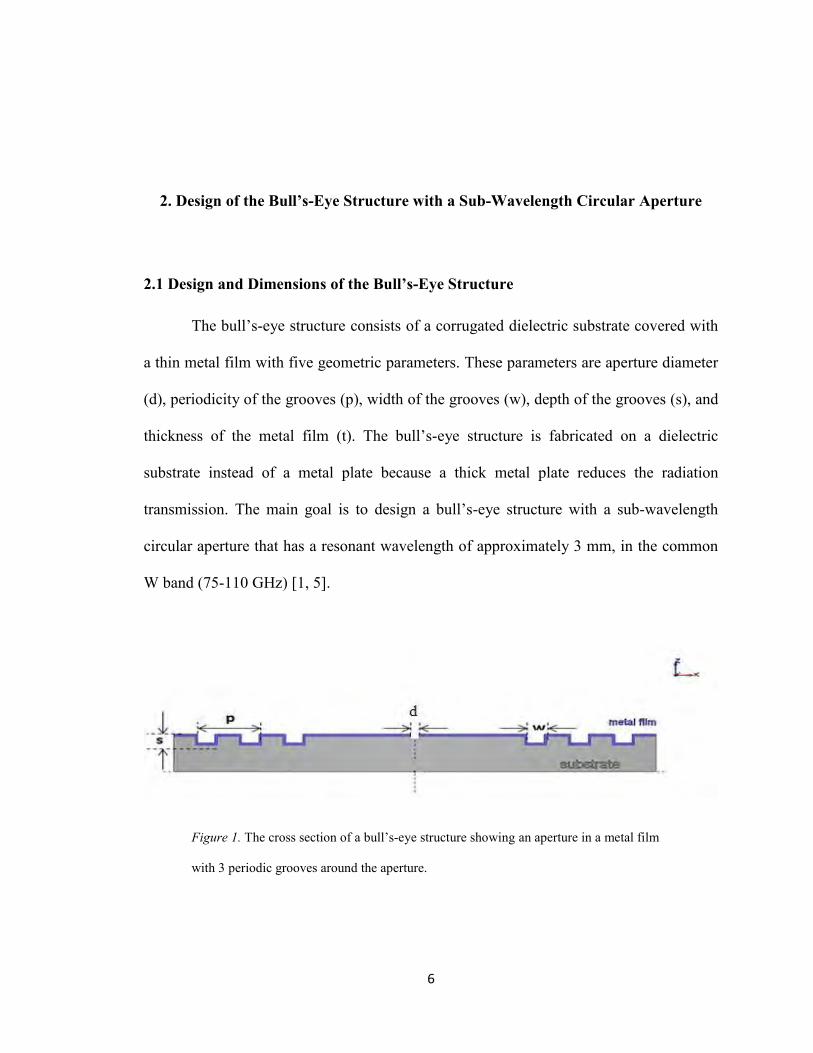
The bull’s-eye structure consists of a corrugated dielectric substrate covered with

a thin metal film with five geometric parameters. These parameters are aperture diameter

(d), periodicity of the grooves (p), width of the grooves (w), depth of the grooves (s), and

thickness of the metal film (t). The bull’s-eye structure is fabricated on a dielectric

substrate instead of a metal plate because a thick metal plate reduces the radiation

transmission. The main goal is to design a bull’s-eye structure with a sub-wavelength

circular aperture that has a resonant wavelength of approximately 3 mm, in the common

W band (75-110 GHz) [1, 5].

Figure 1. The cross section of a bull’s-eye structure showing an aperture in a metal film

with 3 periodic grooves around the aperture.

7

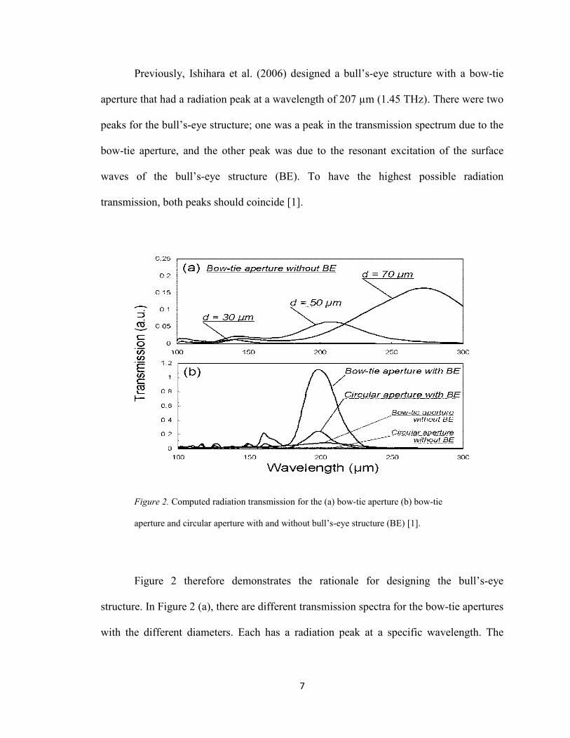
Previously, Ishihara et al. (2006) designed a bull’s-eye structure with a bow-tie

aperture that had a radiation peak at a wavelength of 207 µm (1.45 THz). There were two

peaks for the bull’s-eye structure; one was a peak in the transmission spectrum due to the

bow-tie aperture, and the other peak was due to the resonant excitation of the surface

waves of the bull’s-eye structure (BE). To have the highest possible radiation

transmission, both peaks should coincide [1].

Figure 2. Computed radiation transmission for the (a) bow-tie aperture (b) bow-tie

aperture and circular aperture with and without bull’s-eye structure (BE) [1].

Figure 2 therefore demonstrates the rationale for designing the bull’s-eye

structure. In Figure 2 (a), there are different transmission spectra for the bow-tie apertures

with the different diameters. Each has a radiation peak at a specific wavelength. The

8

bow-tie aperture having the diameter of 50 μm has the peak at the desired wavelength of

207 μm, so this bow-tie aperture was used in the Ishihara et al. (2006) design [1].

In Figure 2 (b), the designed bull’s-eye structure has a peak at the desired design

wavelength (207 μm). For the bull’s-eye structures, the one with a bow-tie aperture and

the one with a circular aperture, high radiation transmission improvements exist

compared to the bow-tie and circular apertures without the bull’s-eye structure.

It should be noted that the bull’s-eye structure with the bow-tie aperture has

higher radiation transmission compared to the bull’s-eye structure without the bow-tie

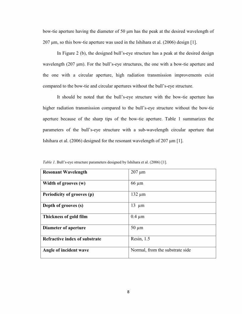
aperture because of the sharp tips of the bow-tie aperture. Table 1 summarizes the

parameters of the bull’s-eye structure with a sub-wavelength circular aperture that

Ishihara et al. (2006) designed for the resonant wavelength of 207 μm [1].

Table 1. Bull’s-eye structure parameters designed by Ishihara et al. (2006) [1].

Resonant Wavelength 207 μm

Width of grooves (w) 66 µm

Periodicity of grooves (p) 132 µm

Depth of grooves (s) 13 µm

Thickness of gold film 0.4 µm

Diameter of aperture 50 µm

Refractive index of substrate Resin, 1.5

Angle of incident wave Normal, from the substrate side

9

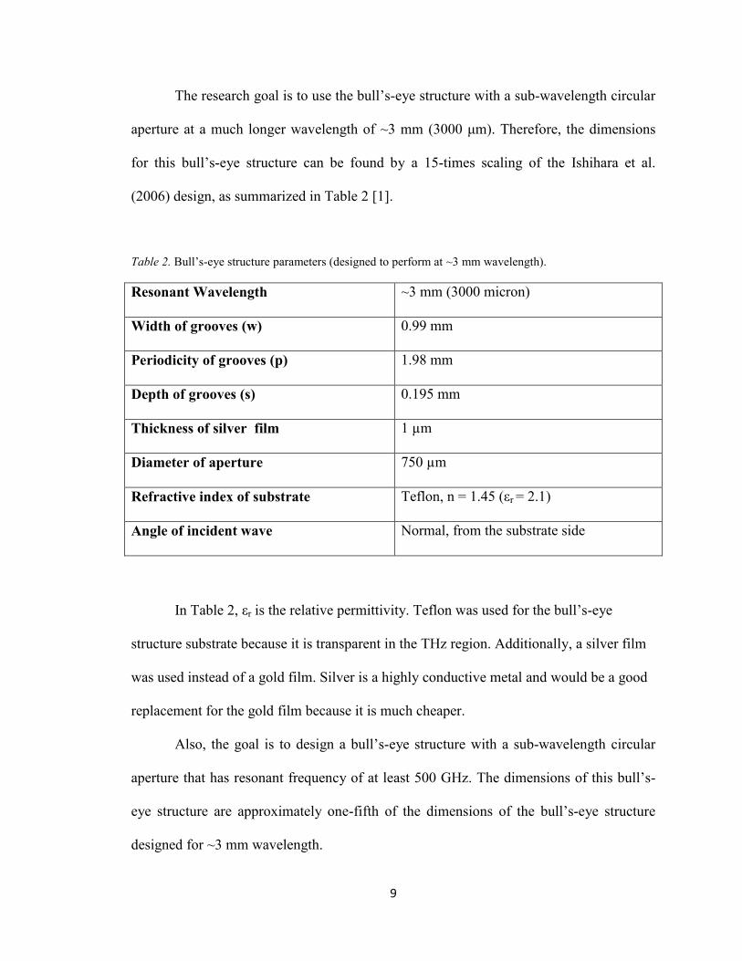
The research goal is to use the bull’s-eye structure with a sub-wavelength circular

aperture at a much longer wavelength of ~3 mm (3000 μm). Therefore, the dimensions

for this bull’s-eye structure can be found by a 15-times scaling of the Ishihara et al.

(2006) design, as summarized in Table 2 [1].

Table 2. Bull’s-eye structure parameters (designed to perform at ~3 mm wavelength).

Resonant Wavelength ~3 mm (3000 micron)

Width of grooves (w) 0.99 mm

Periodicity of grooves (p) 1.98 mm

Depth of grooves (s) 0.195 mm

Thickness of silver film 1 µm

Diameter of aperture 750 µm

Refractive index of substrate Teflon, n = 1.45 (εr = 2.1)


In Table 2, εr is the relative permittivity. Teflon was used for the bull’s-eye

structure substrate because it is transparent in the THz region. Additionally, a silver film

was used instead of a gold film. Silver is a highly conductive metal and would be a good

replacement for the gold film because it is much cheaper.

Also, the goal is to design a bull’s-eye structure with a sub-wavelength circular

aperture that has resonant frequency of at least 500 GHz. The dimensions of this bull’s-

eye structure are approximately one-fifth of the dimensions of the bull’s-eye structure

designed for ~3 mm wavelength.

10

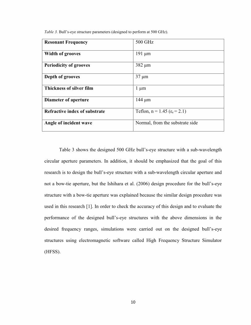
Table 3. Bull’s-eye structure parameters (designed to perform at 500 GHz).

Resonant Frequency 500 GHz

Width of grooves 191 μm

Periodicity of grooves 382 μm

Depth of grooves 37 μm


Diameter of aperture 144 μm



Table 3 shows the designed 500 GHz bull’s-eye structure with a sub-wavelength

circular aperture parameters. In addition, it should be emphasized that the goal of this

research is to design the bull’s-eye structure with a sub-wavelength circular aperture and

not a bow-tie aperture, but the Ishihara et al. (2006) design procedure for the bull’s-eye

structure with a bow-tie aperture was explained because the similar design procedure was

used in this research [1]. In order to check the accuracy of this design and to evaluate the

performance of the designed bull’s-eye structures with the above dimensions in the

desired frequency ranges, simulations were carried out on the designed bull’s-eye

structures using electromagnetic software called High Frequency Structure Simulator

(HFSS).

11

3. Simulation and Fabrication of the Bull’s-Eye Structure with a Sub-Wavelength

Circular Aperture

3.1 Introduction to HFSS

HFSS uses the finite element method (FEM) to solve Maxwell’s equations for the

electromagnetic fields when no analytic solution exists for them. This is particularly true

for complex geometries and boundary conditions. The elements used by HFSS are three

dimensional tetrahedra. HFSS uses a conformal, adaptive system of meshing, meaning

that it creates a large number of elements in the regions where the field shows large

variation, but it uses a smaller number of elements in the regions with lower field

variation. Then HFSS compares the results of the current mesh to the previous mesh until

the solution is converged to the user defined error [16, 17, 18].

3.2 HFSS Settings

3.2.1 Boundary Condition and Excitation

The bull’s-eye structure is first created geometrically within an air-filled box, as

shown in Figure 3. Radiation boundary conditions are assigned to the four sides of the

box. For the radiation boundary condition, no reflection occurs, and the entire radiation

incident on the boundary is absorbed.

12

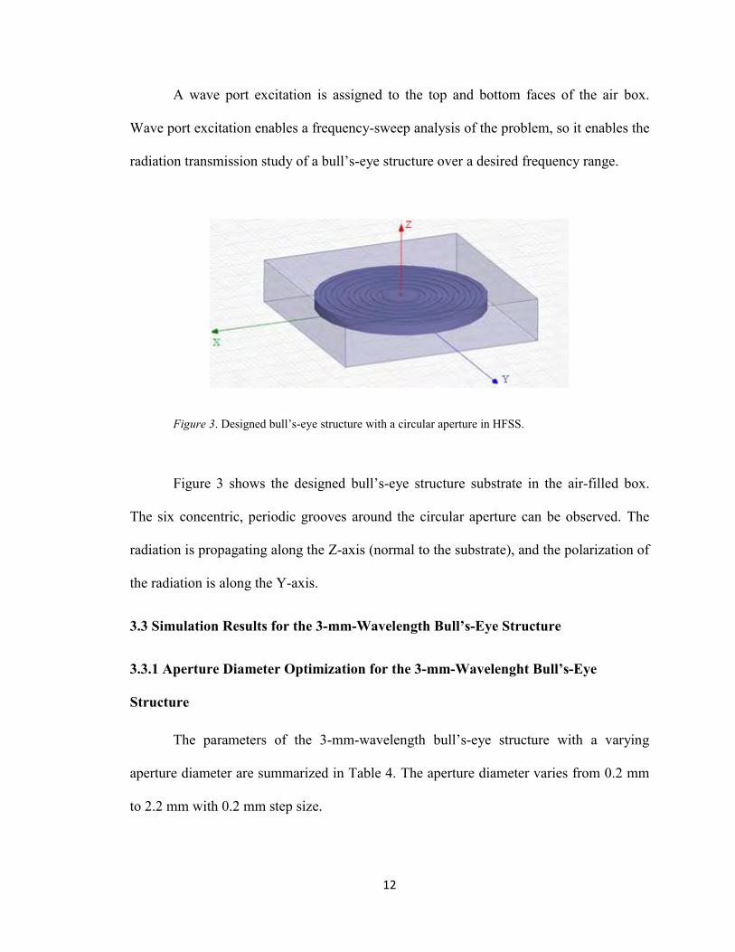
A wave port excitation is assigned to the top and bottom faces of the air box.

Wave port excitation enables a frequency-sweep analysis of the problem, so it enables the

radiation transmission study of a bull’s-eye structure over a desired frequency range.

Figure 3. Designed bull’s-eye structure with a circular aperture in HFSS.

Figure 3 shows the designed bull’s-eye structure substrate in the air-filled box.

The six concentric, periodic grooves around the circular aperture can be observed. The

radiation is propagating along the Z-axis (normal to the substrate), and the polarization of

the radiation is along the Y-axis.

3.3 Simulation Results for the 3-mm-Wavelength Bull’s-Eye Structure

3.3.1 Aperture Diameter Optimization for the 3-mm-Wavelenght Bull’s-Eye

Structure

The parameters of the 3-mm-wavelength bull’s-eye structure with a varying

aperture diameter are summarized in Table 4. The aperture diameter varies from 0.2 mm

to 2.2 mm with 0.2 mm step size.

13

Table 4. 3-mm-wavelength bull's-eye structure parameters (aperture diameter optimization).

Frequency Sweep 90 -100 GHz

Width of grooves (w) 0.99 mm

Periodicity of grooves (p) 1.99 mm

Depth of grooves (s) 0.195 mm

Thickness of silver film (t) 1 µm

Diameter of aperture (d) 0.2-2.2 mm



HFSS allows for the optimization of transmission or other electromagnetic

characteristics by varying geometrical or material parameters. In this case, all the

geometric parameters of the bull’s-eye structure were held constant except the aperture

diameter, which was varied parametrically to maximize the radiation transmission. The

end goal is an aperture diameter which has both high radiation transmission and also

small spatial resolution. Studying the bull’s-eye structure with different aperture

diameters allows for the selection of an aperture diameter which has these desired

features. Also, it should be emphasized that other bull’s-eye parameters, which are depth

of grooves(s), width of grooves (w), periodicity of grooves (p), were held constant

because periodic grooves parameters (s, w, p) are correlated and constrained by Ishihara

et al. (2006) design.

14

Figure 4. Computed radiation transmission for the bull’s-eye structure with different

aperture diameters (d).

As shown in Figure 4, the bull’s-eye structure with an aperture diameter of 0.75

mm has the highest radiation transmission in the 90-100 GHz frequency range. The

bull’s-eye structures with the aperture diameters of 2.2 mm and 1.4 mm have radiation

transmission close to the bull’s-eye structure having an aperture diameter of 0.75 mm, but

the 0.75 mm aperture diameter was selected because it has smaller spatial resolution.

Knife-edge tests were used for measuring the spatial resolution of the bull’s-eye structure

in this research. The knife-edge resolution test is defined by a sharp knife edge that is

0

0.05

0.1

0.15

0.2

0.25

0.3

0.35

0.4

0.45

90 92 94 96 98 100

Tran

smis

sion

(lin

ear)

Freq. (GHz)

d = 0.2 mm

d = 0.4 mm

d = 0.6 mm

d = 0.75 mm

d = 0.8 mm

d = 1 mm

d = 1.2 mm

d = 1.4 mm

d = 1.8 mm

d = 2 mm

d = 2.2 mm

15

laterally displaced so that it blocks from 90% to 10% of the transmitted signal strength

through the aperture (the spatial resolution measurement for the bull’s-eye structure with

an aperture diameter of 0.75 is explained in the fourth chapter) [5].

There are many publications regarding the bull’s-eye structure design in different

spectral regions. They measured the bull’s-eye structures radiation transmission in the

near-field region because the enhanced radiation transmission seen in a bull’s-eye

structure is mainly an effect of evanescent waves, caused by the corrugated metal surface,

transmitting through the aperture. The near-field region of a bull’s-eye structure is

located on the transmission side and within one aperture diameter of the structure. The

evanescent waves are of high magnitude in the near-field region, so the goal of this

research is to study the near-field radiation transmission of the bull’s-eye structure [5].

As the simulations of the bull’s-eye structure evolved, it became evident that the

transmission spectrum was dependent on the distance of the wave ports from the bull’s-

eye structure (this dependence is explained in sections 3.3.2-3.3.4). So the radiation

transmission was computed at three typical distances: (1) 1 mm from the bull’s-eye

structure (~one-third of the excitation wavelength), (2) 0.5 mm from the bull’s-eye

structure, which is located in the near-field region, and (3) 3 mm (= excitation

wavelength) away from the bull’s-eye structure.

3.3.2 3-mm-Wavelength Bull’s-Eye Structure (1mm Distance from Wave Port)

Figure 5 shows the transmission spectrum versus frequency for the bull’s-eye

structure with an aperture diameter of 0.75 mm and a frequency step size of 0.1 GHz.

16

Figure 5. Computed radiation transmission for the 3-mm-wavelength bull’s-eye structure

(1 mm distance from wave port).

In Figure 5, the radiation transmission peak is at 96.6 GHz, which has exactly 15

times longer wavelength than 1.449 THz-the resonant frequency for the bull’s-eye

structure designed by Ishihara et al. (2006). This is gratifying because the other

dimensions used in this structure design are a 15-times scaling of the Ishihara et al.

(2006) design. The radiation transmission is relatively high in the whole frequency range,

and minimum transmission occurs just above 97 GHz [1].

-13

-12

-11

-10

-9

-8

-7

90 91 92 93 94 95 96 97 98 99 100

Tran

smis

sion

(dB

)

Freq. (GHz)

17

Figure 6. Computed E-field magnitude distribution on the x-z plane of the 3-mm-

wavelength bull’s-eye structure (1 mm distance from wave port).

Figure 6 shows the electric field magnitude on both sides of the aperture. The red

color shows the highest E-field magnitude and the blue color shows the lowest E-field

magnitude. As shown in Figure 6, there is no E-field concentration at the aperture exit.

This was surprising because the main reason for designing the bull’s-eye structure is to

have an enhanced E-field at the aperture exit. Although the transmission spectrum seems

to be compatible with the Ishihara et al. (2006) results, the E-field is inconsistent. So the

transmission spectrum was computed at two other distances: 0.5 mm and 3 mm. 0.5 mm

distance was chosen because it is located in the near-field region of the bull’s-eye

structure, and 3 mm was chosen because it is one wavelength away from the bull’s-eye

structure, approaching the far-field [1].

18

3.3.3 3-mm-Wavelength Bull’s-Eye Structure (0.5 mm Distance from Wave Port)

Figure 7 shows the transmission spectrum versus frequency of the bull’s-eye

structure in the near-field region with a frequency step size of 0.5 GHz.


(0.5 mm distance from wave port).

The transmission spectrum in Figure 7 is different from the one shown in Figure

5. For instance, the radiation transmission peak is at 100 GHz in Figure 7. Furthermore,

the radiation transmission in Figure 7 is very low at 92 GHz, much less than the

-30

-25

-20

-15

-10

-5

0

90 91 92 93 94 95 96 97 98 99 100

Tran

smis

sion

(dB

)

Freq. (GHz)

19

minimum in Figure 5. The evanescent waves could be responsible for the difference in

the results because they are stronger in the near-field region of the structure.


wavelength bull’s-eye structure (0.5 mm distance from wave port).

Figure 8 shows the E-field distribution of the bull’s-eye structure as well as the

large E-field at the aperture exit. It can be observed that E-field magnitude is extremely

large exactly below the aperture exit, which is depicted in red color, and should be caused

by the concentration of the surface waves at the center of the structure. In addition, the E-

field spot size at the aperture exit is very small, which can show that the enhanced

radiation of the bull’s-eye structure is a near-field effect, and cannot be observed at the

large distances from the bull’s-eye structure.

20

3.3.4 3-mm-Wavelength Bull’s-Eye Structure (3 mm Distance from Wave Port)

Figure 9 shows the bull’s-eye structure transmission spectrum versus frequency

with a frequency step size of 0.5 GHz at approximately one wavelength away from the

bull’s-eye.


(3 mm distance from wave port).

The transmission spectrum in Figure 9 looks much different than the two previous

spectra at 0.5 mm and 1 mm distances. It is quite constant in the 91-96 GHz frequency

range but is very low near 97 GHz and 99.5 GHz. Also, it should be mentioned that the

-45

-40

-35

-30

-25

-20

-15

-10

-5

90 91 92 93 94 95 96 97 98 99 100

Tran

smis

sion

(dB

)

Freq. (GHz)

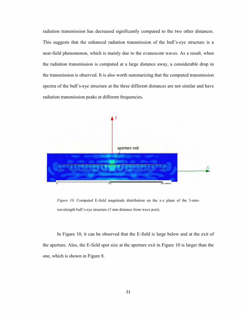
21

radiation transmission has decreased significantly compared to the two other distances.

This suggests that the enhanced radiation transmission of the bull’s-eye structure is a

near-field phenomenon, which is mainly due to the evanescent waves. As a result, when

the radiation transmission is computed at a large distance away, a considerable drop in

the transmission is observed. It is also worth summarizing that the computed transmission

spectra of the bull’s-eye structure at the three different distances are not similar and have

radiation transmission peaks at different frequencies.


wavelength bull’s-eye structure (3 mm distance from wave port).

In Figure 10, it can be observed that the E-field is large below and at the exit of

the aperture. Also, the E-field spot size at the aperture exit in Figure 10 is larger than the

one, which is shown in Figure 8.

22

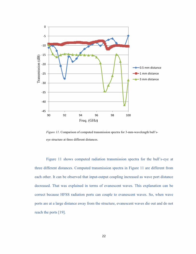
Figure 11. Comparison of computed transmission spectra for 3-mm-wavelength bull’s-

eye structure at three different distances.

Figure 11 shows computed radiation transmission spectra for the bull’s-eye at

three different distances. Computed transmission spectra in Figure 11 are different from

each other. It can be observed that input-output coupling increased as wave port distance

decreased. That was explained in terms of evanescent waves. This explanation can be

correct because HFSS radiation ports can couple to evanescent waves. So, when wave

ports are at a large distance away from the structure, evanescent waves die out and do not

reach the ports [19].

-45

-40

-35

-30

-25

-20

-15

-10

-5

0

90 92 94 96 98 100

Tran

smis

sion

(dB

)

Freq. (GHz)

0.5 mm distance

1 mm distance

3 mm distance

23

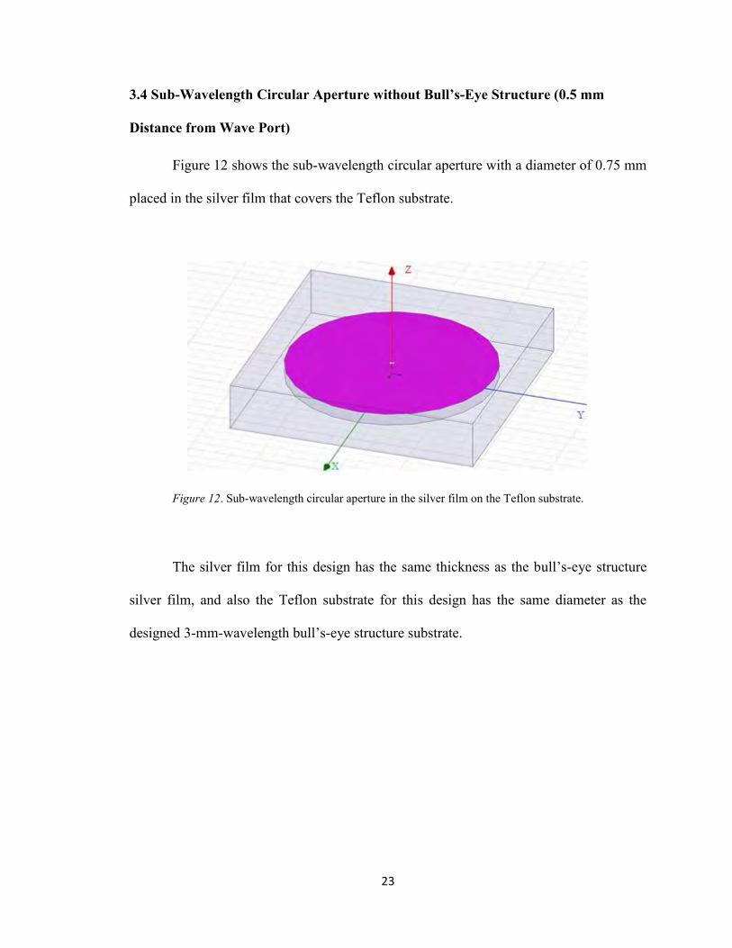
3.4 Sub-Wavelength Circular Aperture without Bull’s-Eye Structure (0.5 mm

Distance from Wave Port)

Figure 12 shows the sub-wavelength circular aperture with a diameter of 0.75 mm

placed in the silver film that covers the Teflon substrate.

Figure 12. Sub-wavelength circular aperture in the silver film on the Teflon substrate.

The silver film for this design has the same thickness as the bull’s-eye structure

silver film, and also the Teflon substrate for this design has the same diameter as the

designed 3-mm-wavelength bull’s-eye structure substrate.

24

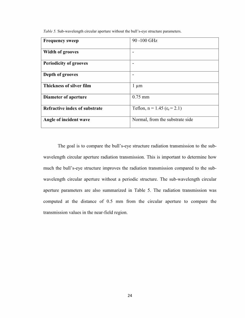
Table 5. Sub-wavelength circular aperture without the bull’s-eye structure parameters.

Frequency sweep 90 -100 GHz

Width of grooves -

Periodicity of grooves -

Depth of grooves -


Diameter of aperture 0.75 mm



The goal is to compare the bull’s-eye structure radiation transmission to the sub-

wavelength circular aperture radiation transmission. This is important to determine how

much the bull’s-eye structure improves the radiation transmission compared to the sub-

wavelength circular aperture without a periodic structure. The sub-wavelength circular

aperture parameters are also summarized in Table 5. The radiation transmission was

computed at the distance of 0.5 mm from the circular aperture to compare the

transmission values in the near-field region.

25

Figure 13. Computed radiation transmission for the sub-wavelength circular aperture

without periodic structure (0.5 mm distance from wave port).

Figure 13 shows the radiation transmission of the sub-wavelength circular

aperture in the silver film on the Teflon substrate. The highest radiation transmission is

close to -15 dB at 99.5 GHz, and the lowest radiation transmission is less than -40 dB. In

addition, the transmission spectrum shows large variation in the 90-100 GHz frequency

range.

-45

-40

-35

-30

-25

-20

-15

90 91 92 93 94 95 96 97 98 99 100

Tran

smis

sion

(dB

)

Freq. (GHz)

26

Figure 14. Radiation transmission comparison of the sub-wavelength circular aperture

with and without bull’s-eye structure in the near-field region.

Figure 14 shows the comparison between the circular aperture and bull’s-eye

structure clearly. The radiation transmission is improved by using concentric, periodic

grooves around the sub-wavelength circular aperture. The bull’s-eye structure radiation

transmission is much higher than the circular aperture except at the frequencies close to

92 GHz, which is not good because the purpose of designing the bull’s-eye structure is to

improve the radiation transmission of the sub-wavelength aperture.

-45

-40

-35

-30

-25

-20

-15

-10

-5

0

90 92 94 96 98 100

Tran

smis

sion

(dB

)

Freq. (GHz)

bull's-eye structure

circular aperture

27

3.5 500 GHz Bull’s-Eye Structure

In the interest of using the bull’s-eye structure for bio spectroscopy, a structure

was designed to perform at 500 GHz. The dimensions of this bull’s-eye structure are

approximately one-fifth of those used in the 3-mm-wavelength design. Transmission

spectrum was computed at 200 μm (~λ/3) distance from the bull’s-eye structure.

Figure 15. Computed radiation transmission of 500 GHz bull’s-eye structure.

Figure 15 shows that the radiation transmission is quite high at 500 GHz and is

close to -10 dB. Also, the radiation transmission is high in the frequency range of 495-

510 GHz. The dimensions of this designed bull’s-eye structure are approximately a three-

-40

-35

-30

-25

-20

-15

-10

-5

450 460 470 480 490 500 510 520 530 540 550

Tran

smis

sion

(dB

)

Freq. (GHz)

28

times scaling of Ishihara et al. (2006) design and Figure 15 shows that these dimensions

are the proper values for the 500 GHz bull’s-eye structure design because high radiation

transmission is observed at the design frequency [1].

Figure 16. Computed E-field magnitude distribution on the x-z plane of the 500 GHz

bull’s-eye structure.

Figure 16 shows the E-field magnitude at the aperture exit. The E-field is

extremely large at the center of the bull’s-eye structure below the aperture because of the

radial concentration of the surface waves. In addition, the E-field spot size at the aperture

exit is relatively small.

3.6 Fabrication of 3-mm-Wavelength Bull’s-Eye Structure

The periodic grooves in the 3-mm-wavelength bull’s-eye structure were created

with a CNC lathe on a Teflon or high-density polyethylene (HDPE) substrate. Both of

these substrate materials are transparent in the THz region. Also, they are readily

available materials, and have good machining properties. After the CNC machining was

29

complete, the corrugated substrate was separated from the Teflon rod. A Silver film

having 1 μm thickness was deposited on the substrate by thermal evaporation. Then the

central circular aperture was made in the silver film using a 0.75 mm drill bit.

The thickness of the silver film was determined by the requirement that it should

be large enough to prevent radiation from transmitting through it.

Figure 17. Fabricated bull’s-eye structure with six periodic grooves covered with the

silver film.

Figure 17 depicts the fabricated bull’s-eye structure with a sub-wavelength

circular aperture. An experiment was needed to determine the spatial resolution of the

structure, which is discussed next.

30

4. Experimental Measurement

4.1 Spatial Resolution Measurement Method

The quality of the fabricated 3-mm-wavelength bull’s-eye structure was

determined by measuring its spatial resolution. This was done using the knife-edge

resolution technique, and this technique is defined as the lateral displacement of a sharp

knife edge so that 90% to 10% of the transmitted signal strength is allowed through an

aperture [5].

4.2 Knife-Edge Test

A knife-edge test was conducted to measure the spatial resolution of the bull’s-

eye structure by moving a sharp knife edge across the circular aperture of the bull’s-eye

structure. The spatial resolution was measured was measured in two directions (X-axis

and Y-axis).

31

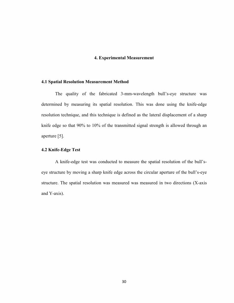
Figure 18. Knife-edge test set up for measuring the bull’s-eye structure spatial resolution.

For this test, the radiative source is a 100 GHz voltage-controlled Gunn oscillator

with the pyramidal feed horn. The polarization of the Gunn oscillator was in the vertical

direction (Y-axis). The source was chopped at 100 KHz, and the radiation was

transmitted through a spherical lens with the bull’s-eye structure pointed toward the wave

guide-mounted Schottky-diode detector. The detector’s wave guide was a corrugated

conical feed horn. The corrugation of the conical feed horn reduces the side lobes.

A spherical lens was used behind the bull’s-eye structure to collimate the

Gaussian beam of the source. Therefore, there is much less radiation leakage around the

sides of the lens, and the majority of the radiation detected is the radiation that is

transmitted through the bull’s-eye structure. The substrate side of the bull’s-eye structure

32

faces the source, and the wave is normally incident on this side. The detector is placed at

the closest possible distance from the aperture (~2 mm) because the bull’s-eye structure

radiation transmission is high in the near-field region.

4.3 Results of the Knife-Edge Test: Spatial Resolution Curves

By using the knife-edge resolution definition, the spatial resolution can be

measured along the X and Y axes from the measured transmission curves.

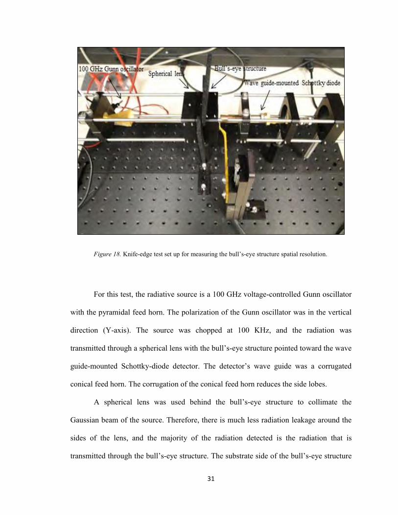
Figure 19. Measured spatial resolution curve along the X-axis.

The spatial resolution curve along the X-axis is shown in Figure 19. The signal is

approximately constant out to X = 0.6 mm and has its highest strength near X = 0, as

expected. When the knife edge starts moving across the aperture, there is a sharp drop in

the signal strength until the knife edge covers the aperture completely. Then the signal

0

10

20

30

40

50

60

70

80

90

0 0.5 1 1.5 2

Tran

smis

sion

(a.u

)

X (mm)

0.7 mm

33

strength goes approximately to zero. Based on the definition of the knife-edge resolution,

Figure 19 shows that the knife edge displacement from 90% to 10% of the signal strength

is approximately 0.7 mm. This means that the spatial resolution was 0.7 mm along the X-

axis, which is approximately λ/4 at 100 GHz (3 mm wavelength).

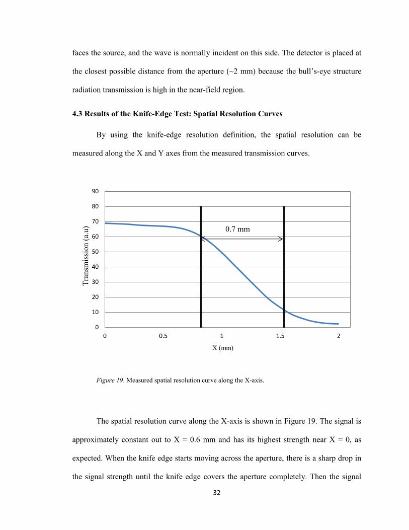
Figure 20. Measured spatial resolution curve along the Y-axis.

The spatial resolution curve along the Y-axis was not as well behaved as along the X-

axis. There are two differences in Figure 20 in comparison to Figure 19. The first one is

that there is no initial constant signal strength region in Figure 20 as was seen in Figure

19. The second difference is that the signal strength in Figure 20 does not go to zero even

when the knife edge covers the aperture completely; however, one can still observe the

sharp drop in the signal strength when the knife edge starts covering the aperture. These

0

10

20

30

40

50

60

70

80

90

0 0.5 1 1.5 2

Tran

smis

sion

(a.u

)

Y (mm)

1 mm

34

differences could be caused by the leakage around the lens sides. Although the radiation

was collimated by using a spherical lens behind the bull’s-eye structure and covering the

lens holder sides with the absorbers, radiation can still leak around the lens sides.

Moreover, the obtained spatial resolution along the Y-axis is ~1 mm, which is λ/3

at 100 GHz, so the obtained results show that the fabricated bull’s-eye structure has ~λ/4

spatial resolution along the X-axis and λ/3 spatial resolution along the Y-axis. However,

the fabricated bull’s-eye structure probably has the better spatial resolution than this

because the detector had to be placed at ~2 mm distance from the bull’s-eye structure

since the detector was physically large compared to the wavelength of radiation. Because

of this, the detector could not be placed less than two millimeters from the bull’s-eye

structure [5].

Finally, many difficulties were faced and overcome pertaining to the knife-edge

test. The first one was a distance of detector from the bull’s-eye structure. By bringing

the detector to the closest possible distance from bull’-eye, obtained results improved

considerably. Other issue was radiation leakage from lens holder sides. The main reason

for radiation leakage from lens holder sides was the Gaussian beam shape of wave source

radiation, so a spherical lens was used behind the bull’s-eye to collimate radiation and

reduce leakage of radiation. To have the lowest amount of radiation leakage, lens holder

sides were covered with absorbers. Also, a large-area detector was used for the knife-

edge experiment. Detector can be placed at a closer distance from bull’s-eye if it is

physically smaller. It is recommended to use a physically smaller detector in the near-

field region of bull’s-eye structure for future works because that results in smaller

measured spatial resolution.

35

5. Design and Simulation of the 100 GHz Reflective Probe

5.1 Probe Applications

The water content of cancerous and burnt tissues is often higher than in healthy

tissue, so these tissues have higher energy absorption and higher reflectivity compared to

healthy tissues in the THz region. This higher energy absorption and reflectivity of these

tissues enables their detection by using a reflective probe [20].

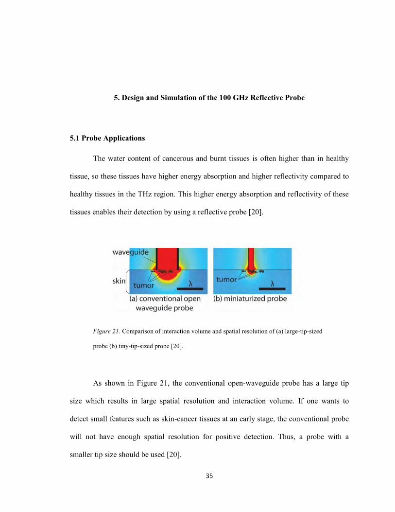
Figure 21. Comparison of interaction volume and spatial resolution of (a) large-tip-sized

probe (b) tiny-tip-sized probe [20].

As shown in Figure 21, the conventional open-waveguide probe has a large tip

size which results in large spatial resolution and interaction volume. If one wants to

detect small features such as skin-cancer tissues at an early stage, the conventional probe

will not have enough spatial resolution for positive detection. Thus, a probe with a

smaller tip size should be used [20].

36

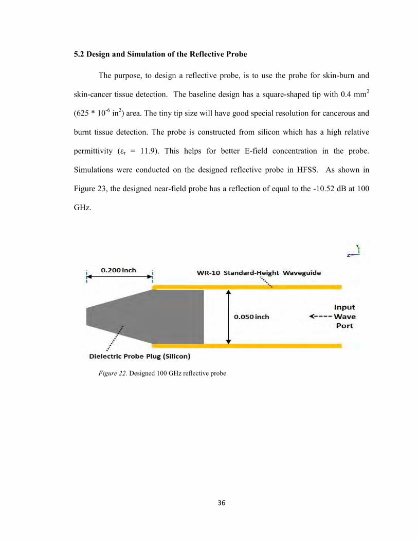
5.2 Design and Simulation of the Reflective Probe

The purpose, to design a reflective probe, is to use the probe for skin-burn and

skin-cancer tissue detection. The baseline design has a square-shaped tip with 0.4 mm2

(625 * 10-6 in2) area. The tiny tip size will have good special resolution for cancerous and

burnt tissue detection. The probe is constructed from silicon which has a high relative

permittivity (εr = 11.9). This helps for better E-field concentration in the probe.

Simulations were conducted on the designed reflective probe in HFSS. As shown in

Figure 23, the designed near-field probe has a reflection of equal to the -10.52 dB at 100

GHz.

Figure 22. Designed 100 GHz reflective probe.

37

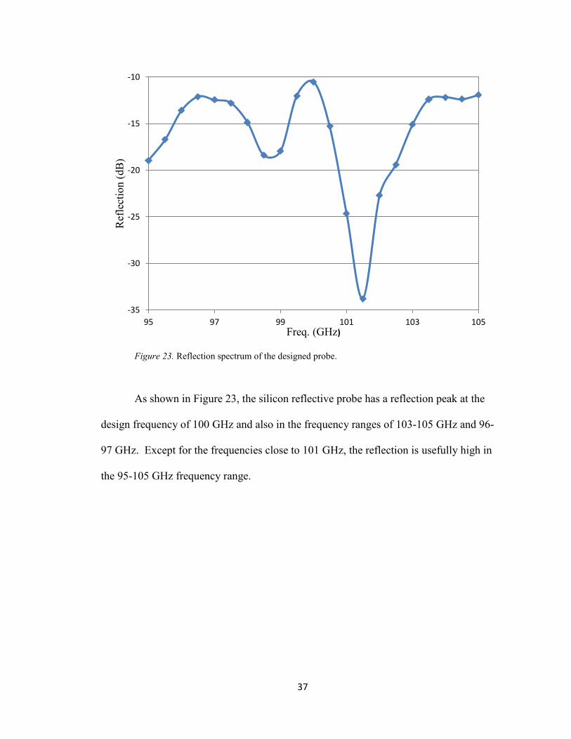
Figure 23. Reflection spectrum of the designed probe.

As shown in Figure 23, the silicon reflective probe has a reflection peak at the

design frequency of 100 GHz and also in the frequency ranges of 103-105 GHz and 96-

97 GHz. Except for the frequencies close to 101 GHz, the reflection is usefully high in

the 95-105 GHz frequency range.

-35

-30

-25

-20

-15

-10

95 97 99 101 103 105

Ref

lect

ion

(dB

)

Freq. (GHz)

38

Figure 24. Computed E-field magnitude distribution on the x-z plane of the probe at 100 GHz (polarization

direction is along the Y-axis).

Figure 25. Computed E-field magnitude distribution on the x-y plane of the probe at 100

GHz, 1 μm away from the probe tip.

Figures 24-25 show the E-field magnitude distribution of the probe in two

different planes. The wave propagation can be observed in the probe in Figure 24. Figure

24 also shows a highly concentrated E-field in the probe because it is constructed from

silicon. For instance, if the probe would be constructed from Teflon, such high E-field

magnitude distribution in the probe could not be observed. Figure 25 shows that the E-

field concentrates at the probe tip with the small spatial resolution.

39

6. Conclusion

A bull’s-eye structure with a sub-wavelength circular aperture was designed to

perform at a wavelength of ~3 mm in W band (75-110 GHz). This bull’s-eye structure

can be used for skin-tissue detection, such as detecting melanoma. Simulations were

carried out on the 3D model of the bull’s-eye structure in HFSS. The simulation results

show the computed transmission spectra for the designed bull’s-eye structure. The

transmission spectrum was computed for a 3-mm-wavelength bull’s-eye structure at three

different distances (0.5 mm, 1 mm, and 3mm). The three computed transmission spectra

were different from each other, and a considerable drop in the computed radiation

transmission magnitude was observed at the distance of 3 mm compared to that computed

at the other two distances. This is because the enhanced radiation transmission of the

bull’s-eye structure is a near-field effect.

A 3-mm-wavelength bull’s-eye structure was fabricated and measured for its

spatial resolution by the knife-edge test. The detector was placed at the ~2 mm distance

from the bull’s-eye structure. By conducting the knife-edge test at 100 GHz, a resolution

of 0.7 mm (~λ/4) was obtained along the X-axis and 1 mm was obtained along the Y-

axis. The difference in the obtained spatial resolution results can be because of the

radiation leakage around the lens sides. Also, the detector was physically large compared

to the radiation wavelength, so a better resolution would likely have been obtained if a

smaller detector was used in near-field region of the bull’s-eye structure.

40

Also, a bull’s-eye structure with a sub-wavelength circular aperture was designed

to have resonant frequency of at least 500 GHz. This bull’s-eye structure can be used in

biological sensing and detection. Then the 3D model of the 500 GHz bull’s-eye structure

was simulated in HFSS. The obtained transmission spectrum for the 500 GHz bull’s-eye

structure shows that the designed bull’s-eye structure has high radiation transmission in

the 500-510 GHz frequency range.

Finally a silicon reflective probe was designed to perform at 100 GHz. The design

probe had a tiny tip with an area of 0.4 mm2. This probe with a tiny tip can be used for

detection of small features such as skin burn and melanoma. The probe was constructed

from silicon because it has high relative permittivity and concentrates the E-field in the

probe. The obtained results from the simulation of the reflective probe in HFSS show that

the probe has high reflection at 100 GHz. Also, the E-field at the probe tip has large

magnitude and small spot size.

41

Appendix I. BobCAD-CAM Job Creation

Introduction

BobCAD-CAM is a software tool for designing 3D parts and creating G-code for

CNC fabrication. The main advantage of using BobCAD is that it allows importing CAD

files designed with other software, such as SolidWorks and AutoCAD. BobCAD is

mainly used for programming G-code for CNC lathe and milling machines [21].

Milling

BobCAD-CAM can be used for 2- and 3-axis milling operations where it provides

a user with a large number of operations for programming G-code for complicated

geometries. For example, engraving, profiling, pocketing, and plunge roughing are

possible milling operations, and can be done with control of several other machining

parameters, such as stock geometry, milling tool data, cutting feed rate, and plunge feed

rate [21].

Lathe

The lathe is used for manufacturing a part which is axisymmetric. For parts to be

cut on the lathe and designed in BobCAD, it is required to draw the 2D cross section

(profile) of the part in the top left quadrant of drawing plane. However, BobCAD does

not have the ability to import data points for these profiles. Instead, SolidWorks can be

42

used for importing such data points. The profile is simply drawn in SolidWorks and can

be extruded along its normal vector to become the 3D part because BobCAD cannot

import 2D parts drawn in SolidWorks. Then the edge of the 3D part can be extracted with

a function in BobCAD to obtain the 2D profile. For more information regarding lathe

drawing, one can watch the training videos available in the THz sensors group dropbox

folder [22, 23].

Post-Processor

The format of G-code produced by BobCAD is controlled by a post processor,

and different CNC machines have different controllers. In order to have the right G-code

format for a specific controller, the correct post-processor should be used. The updated

post-processors can be downloaded directly from the BobCAD website. Both CNC

machines in the THz sensors group have Mach 3 controllers, and the updated Mach 3

post-processors can be downloaded from the BobCAD website [22, 23, 24].

To produce G-code in BobCAD for running a CNC machine, there are several

steps which should be taken. First, a part is designed in BobCAD. Then a set of

operations is selected for fabricating the part. After that, the G-code is posted in BobCAD

and saved for running the appropriate CNC machine. As an example of the different steps

required to program G-code for a desired geometry, the 3-mm-wavelength bull’s-eye

fabrication procedure in BobCAD is explained.

43

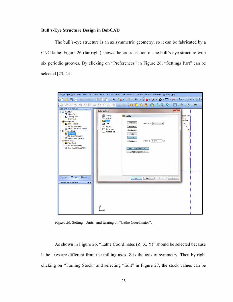
Bull’s-Eye Structure Design in BobCAD

The bull’s-eye structure is an axisymmetric geometry, so it can be fabricated by a

CNC lathe. Figure 26 (far right) shows the cross section of the bull’s-eye structure with

six periodic grooves. By clicking on “Preferences” in Figure 26, “Settings Part” can be

selected [23, 24].

Figure 26. Setting “Units” and turning on “Lathe Coordinates”.

As shown in Figure 26, “Lathe Coordinates (Z, X, Y)” should be selected because

lathe axes are different from the milling axes. Z is the axis of symmetry. Then by right

clicking on “Turning Stock” and selecting “Edit” in Figure 27, the stock values can be

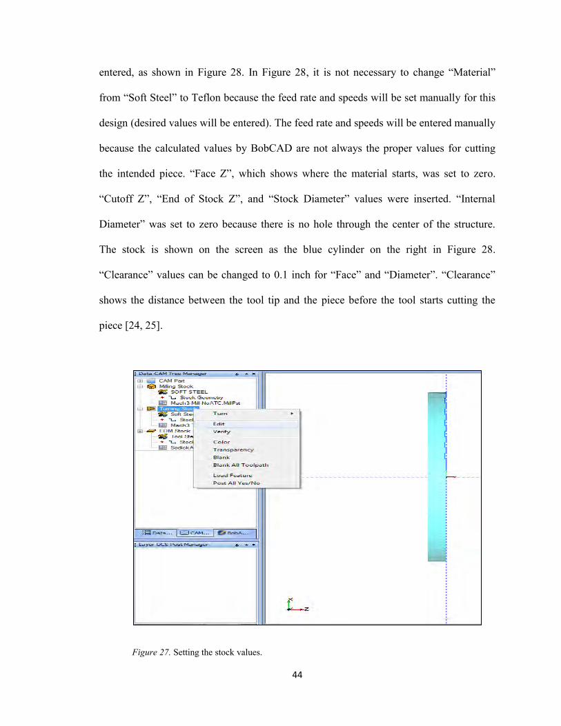
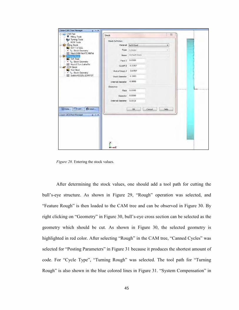
44

entered, as shown in Figure 28. In Figure 28, it is not necessary to change “Material”

from “Soft Steel” to Teflon because the feed rate and speeds will be set manually for this

design (desired values will be entered). The feed rate and speeds will be entered manually

because the calculated values by BobCAD are not always the proper values for cutting

the intended piece. “Face Z”, which shows where the material starts, was set to zero.

“Cutoff Z”, “End of Stock Z”, and “Stock Diameter” values were inserted. “Internal

Diameter” was set to zero because there is no hole through the center of the structure.

The stock is shown on the screen as the blue cylinder on the right in Figure 28.

“Clearance” values can be changed to 0.1 inch for “Face” and “Diameter”. “Clearance”

shows the distance between the tool tip and the piece before the tool starts cutting the

piece [24, 25].

Figure 27. Setting the stock values.

45

Figure 28. Entering the stock values.

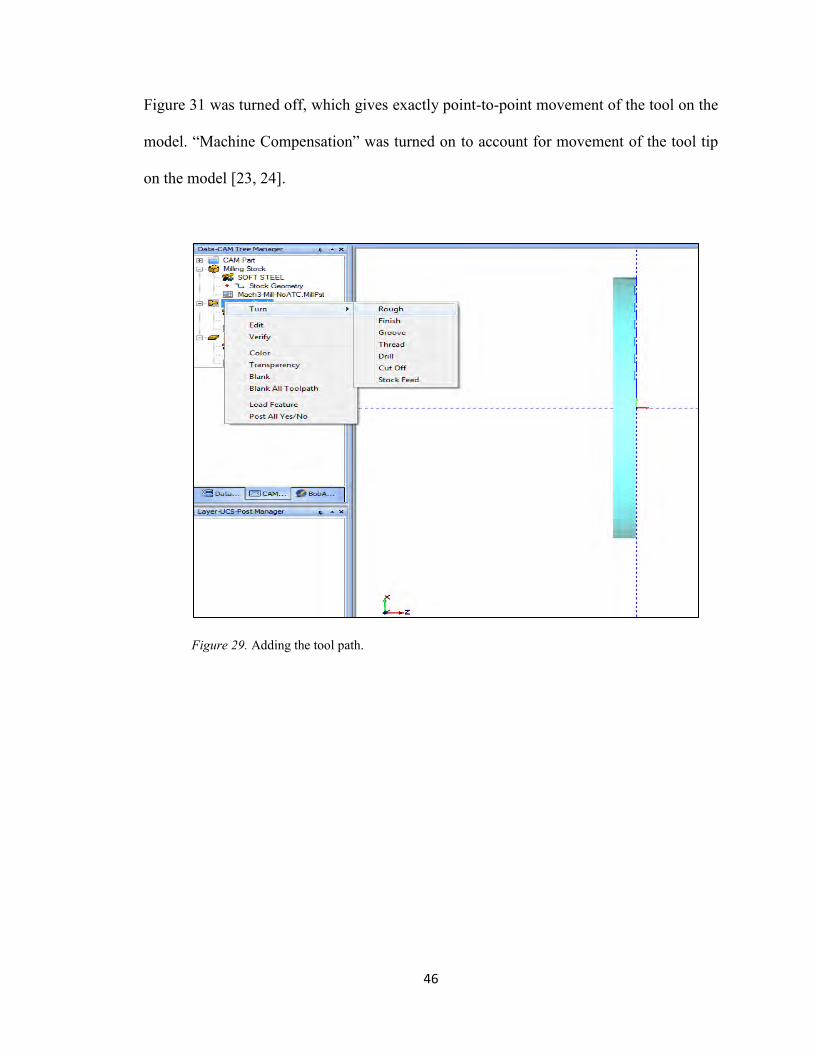
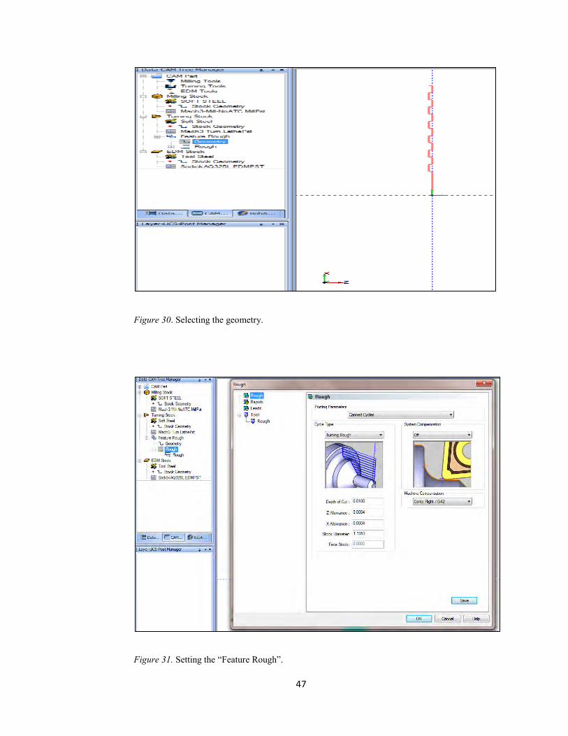
After determining the stock values, one should add a tool path for cutting the

bull’s-eye structure. As shown in Figure 29, “Rough” operation was selected, and

“Feature Rough” is then loaded to the CAM tree and can be observed in Figure 30. By

right clicking on “Geometry” in Figure 30, bull’s-eye cross section can be selected as the

geometry which should be cut. As shown in Figure 30, the selected geometry is

highlighted in red color. After selecting “Rough” in the CAM tree, “Canned Cycles” was

selected for “Posting Parameters” in Figure 31 because it produces the shortest amount of

code. For “Cycle Type”, “Turning Rough” was selected. The tool path for “Turning

Rough” is also shown in the blue colored lines in Figure 31. “System Compensation” in

46

Figure 31 was turned off, which gives exactly point-to-point movement of the tool on the

model. “Machine Compensation” was turned on to account for movement of the tool tip

on the model [23, 24].

Figure 29. Adding the tool path.

47

Figure 30. Selecting the geometry.

Figure 31. Setting the “Feature Rough”.

48

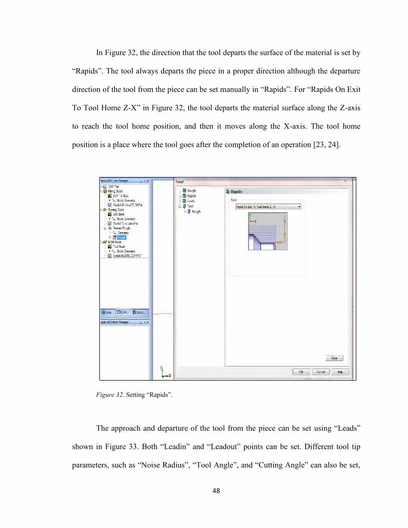
In Figure 32, the direction that the tool departs the surface of the material is set by

“Rapids”. The tool always departs the piece in a proper direction although the departure

direction of the tool from the piece can be set manually in “Rapids”. For “Rapids On Exit

To Tool Home Z-X” in Figure 32, the tool departs the material surface along the Z-axis

to reach the tool home position, and then it moves along the X-axis. The tool home

position is a place where the tool goes after the completion of an operation [23, 24].

Figure 32. Setting “Rapids”.

The approach and departure of the tool from the piece can be set using “Leads”

shown in Figure 33. Both “Leadin” and “Leadout” points can be set. Different tool tip

parameters, such as “Noise Radius”, “Tool Angle”, and “Cutting Angle” can also be set,

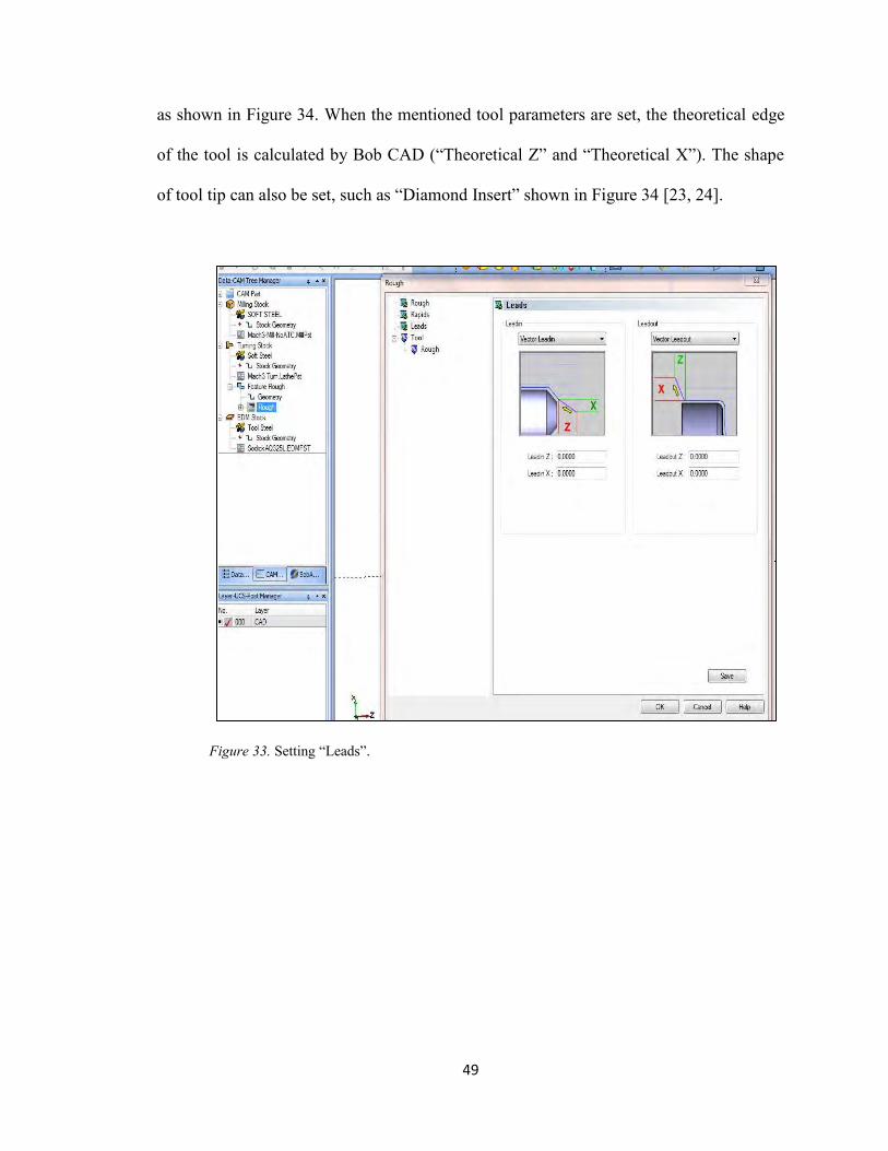
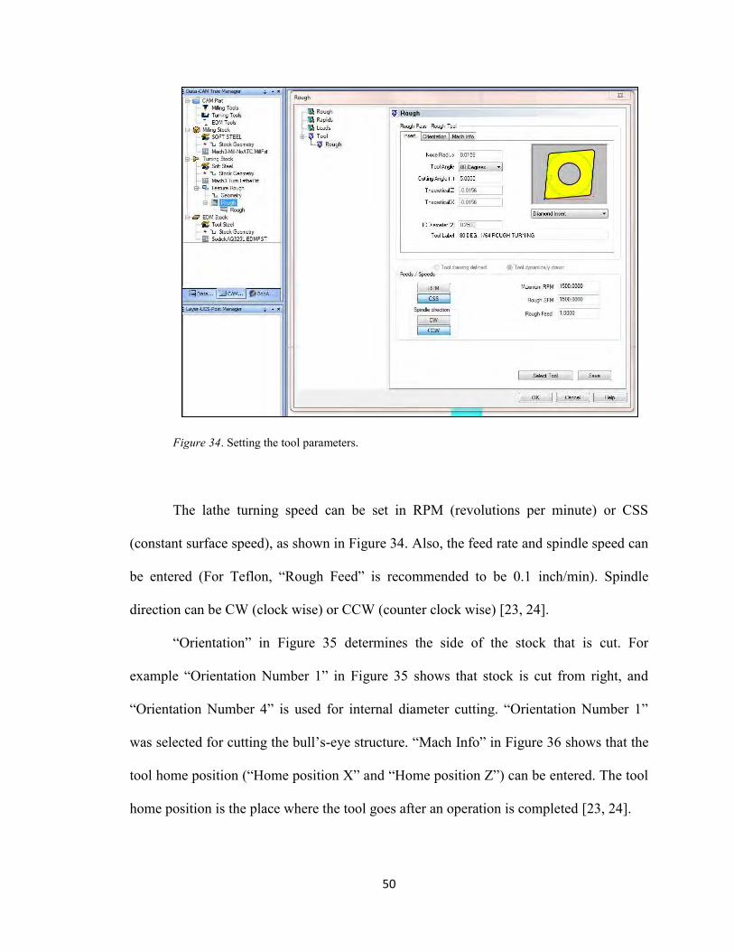
49

as shown in Figure 34. When the mentioned tool parameters are set, the theoretical edge

of the tool is calculated by Bob CAD (“Theoretical Z” and “Theoretical X”). The shape

of tool tip can also be set, such as “Diamond Insert” shown in Figure 34 [23, 24].

Figure 33. Setting “Leads”.

50

Figure 34. Setting the tool parameters.

The lathe turning speed can be set in RPM (revolutions per minute) or CSS

(constant surface speed), as shown in Figure 34. Also, the feed rate and spindle speed can

be entered (For Teflon, “Rough Feed” is recommended to be 0.1 inch/min). Spindle

direction can be CW (clock wise) or CCW (counter clock wise) [23, 24].

“Orientation” in Figure 35 determines the side of the stock that is cut. For

example “Orientation Number 1” in Figure 35 shows that stock is cut from right, and

“Orientation Number 4” is used for internal diameter cutting. “Orientation Number 1”

was selected for cutting the bull’s-eye structure. “Mach Info” in Figure 36 shows that the

tool home position (“Home position X” and “Home position Z”) can be entered. The tool

home position is the place where the tool goes after an operation is completed [23, 24].

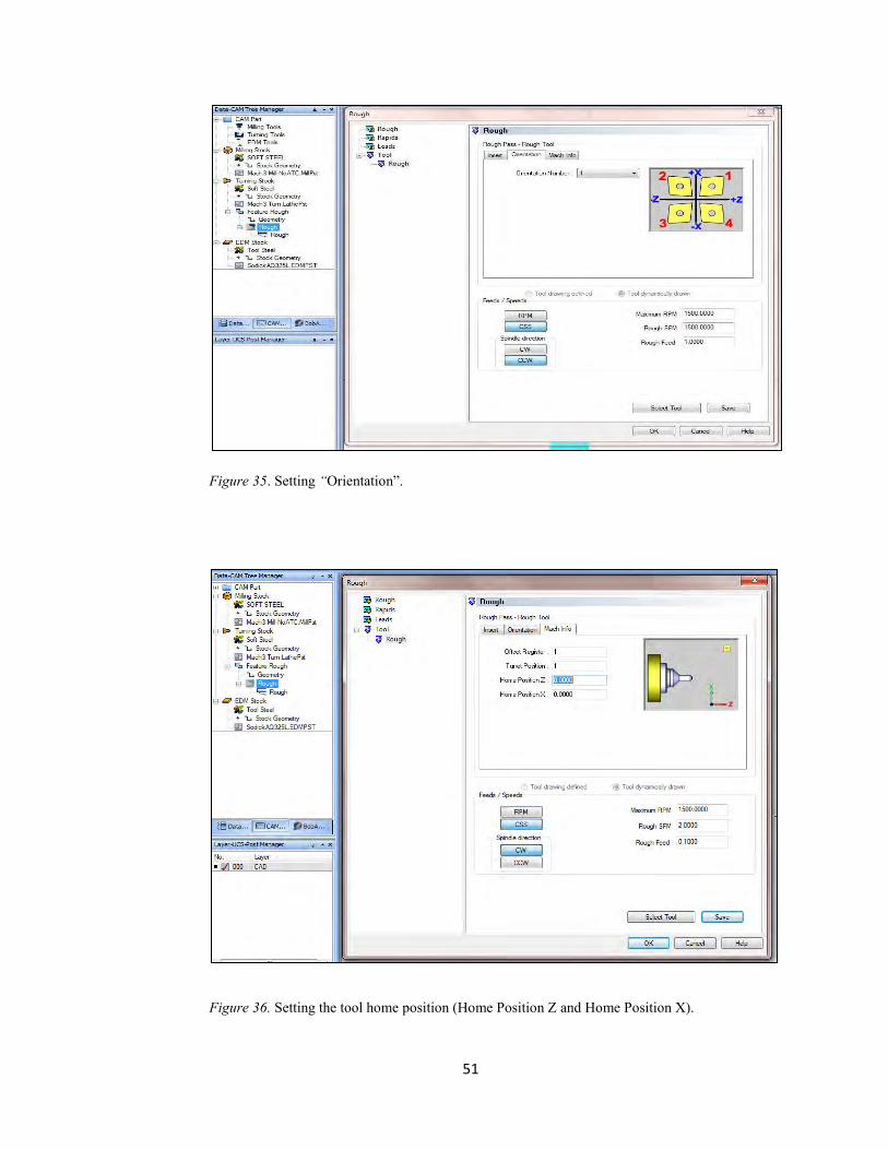
51

Figure 35. Setting “Orientation”.

Figure 36. Setting the tool home position (Home Position Z and Home Position X).

52

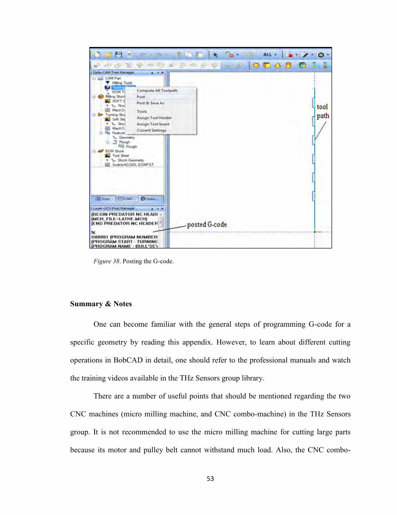
In Figure 37, the Mach 3 post-processor was selected because a lathe CNC

machine with the Mach 3 controller was used for cutting the structure. After selecting the

post-processor, the G-code can be posted by right clicking on “Turning Tools”, as shown

in Figure 38. The tool path on the bull’s-eye structure is shown in green in Figures 37-38

[23, 24].

Figure 37. Selecting the post-processor.

53

Figure 38. Posting the G-code.

Summary & Notes

One can become familiar with the general steps of programming G-code for a

specific geometry by reading this appendix. However, to learn about different cutting

operations in BobCAD in detail, one should refer to the professional manuals and watch

the training videos available in the THz Sensors group library.

There are a number of useful points that should be mentioned regarding the two

CNC machines (micro milling machine, and CNC combo-machine) in the THz Sensors

group. It is not recommended to use the micro milling machine for cutting large parts

because its motor and pulley belt cannot withstand much load. Also, the CNC combo-

54

machine controller cannot be connected to a laptop because the necessary USB cable

connection can vibrate too loose when the machine is in operation, which results in a

disconnection between the laptop and CNC machine controller. So a desktop computer

should be used for running the CNC combo-machine. Any other observation or

recommendations regarding the design, programming or operation of the machines

should be added to this document and posted for future operators.

Prior to any operation of the mills or lathes, the operator must have documented

safety training appropriate to the task. The operator is also responsible for the safety of

any other individuals in the immediate area around the machines.

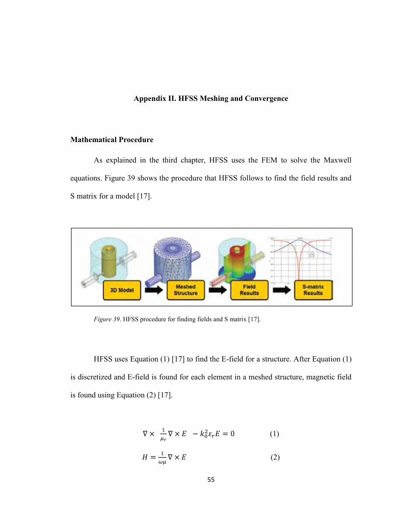
55

Appendix II. HFSS Meshing and Convergence

Mathematical Procedure

As explained in the third chapter, HFSS uses the FEM to solve the Maxwell

equations. Figure 39 shows the procedure that HFSS follows to find the field results and

S matrix for a model [17].

Figure 39. HFSS procedure for finding fields and S matrix [17].

HFSS uses Equation (1) [17] to find the E-field for a structure. After Equation (1)

is discretized and E-field is found for each element in a meshed structure, magnetic field

is found using Equation (2) [17].

(1)

(2)

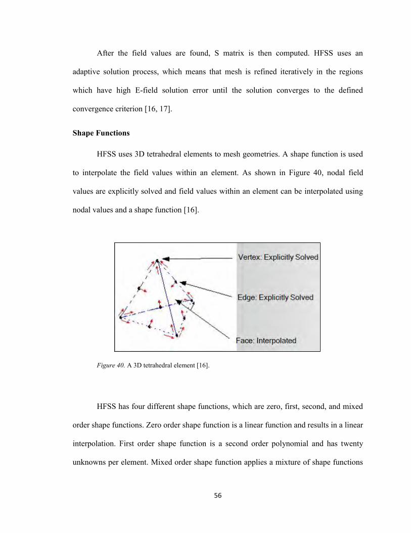
56

After the field values are found, S matrix is then computed. HFSS uses an

adaptive solution process, which means that mesh is refined iteratively in the regions

which have high E-field solution error until the solution converges to the defined

convergence criterion [16, 17].

Shape Functions

HFSS uses 3D tetrahedral elements to mesh geometries. A shape function is used

to interpolate the field values within an element. As shown in Figure 40, nodal field

values are explicitly solved and field values within an element can be interpolated using

nodal values and a shape function [16].

Figure 40. A 3D tetrahedral element [16].

HFSS has four different shape functions, which are zero, first, second, and mixed

order shape functions. Zero order shape function is a linear function and results in a linear

interpolation. First order shape function is a second order polynomial and has twenty

unknowns per element. Mixed order shape function applies a mixture of shape functions

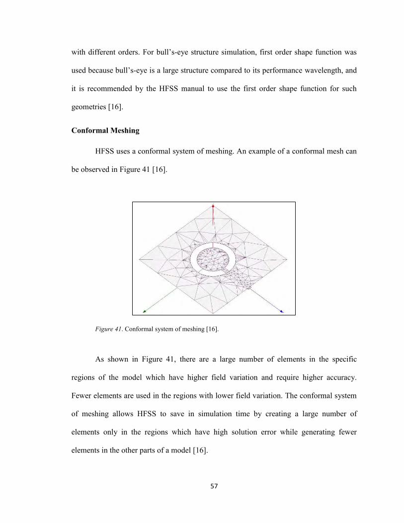
57

with different orders. For bull’s-eye structure simulation, first order shape function was

used because bull’s-eye is a large structure compared to its performance wavelength, and

it is recommended by the HFSS manual to use the first order shape function for such

geometries [16].

Conformal Meshing

HFSS uses a conformal system of meshing. An example of a conformal mesh can

be observed in Figure 41 [16].

Figure 41. Conformal system of meshing [16].

As shown in Figure 41, there are a large number of elements in the specific

regions of the model which have higher field variation and require higher accuracy.

Fewer elements are used in the regions with lower field variation. The conformal system

of meshing allows HFSS to save in simulation time by creating a large number of

elements only in the regions which have high solution error while generating fewer

elements in the other parts of a model [16].

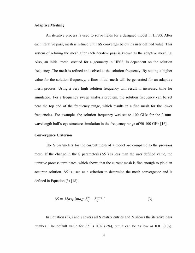
58

Adaptive Meshing

An iterative process is used to solve fields for a designed model in HFSS. After

each iterative pass, mesh is refined until S converges below its user defined value. This

system of refining the mesh after each iterative pass is known as the adaptive meshing.

Also, an initial mesh, created for a geometry in HFSS, is dependent on the solution

frequency. The mesh is refined and solved at the solution frequency. By setting a higher

value for the solution frequency, a finer initial mesh will be generated for an adaptive

mesh process. Using a very high solution frequency will result in increased time for

simulation. For a frequency sweep analysis problem, the solution frequency can be set

near the top end of the frequency range, which results in a fine mesh for the lower

frequencies. For example, the solution frequency was set to 100 GHz for the 3-mm-

wavelength bull’s-eye structure simulation in the frequency range of 90-100 GHz [16].

Convergence Criterion

The S parameters for the current mesh of a model are compared to the previous

mesh. If the change in the S parameters ( ) is less than the user defined value, the

iterative process terminates, which shows that the current mesh is fine enough to yield an

accurate solution. is used as a criterion to determine the mesh convergence and is

defined in Equation (3) [18].

(3)

In Equation (3), i and j covers all S matrix entries and N shows the iterative pass

number. The default value for is 0.02 (2%), but it can be as low as 0.01 (1%).

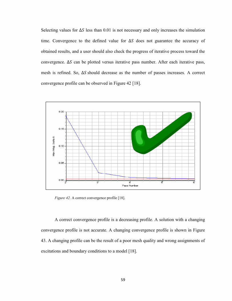
59

Selecting values for less than 0.01 is not necessary and only increases the simulation

time. Convergence to the defined value for does not guarantee the accuracy of

obtained results, and a user should also check the progress of iterative process toward the

convergence. can be plotted versus iterative pass number. After each iterative pass,

mesh is refined. So, should decrease as the number of passes increases. A correct

convergence profile can be observed in Figure 42 [18].

Figure 42. A correct convergence profile [18].

A correct convergence profile is a decreasing profile. A solution with a changing

convergence profile is not accurate. A changing convergence profile is shown in Figure

43. A changing profile can be the result of a poor mesh quality and wrong assignments of

excitations and boundary conditions to a model [18].

60

Figure 43. A changing convergence profile [18].

In the case of having a changing convergence profile for a solution, the obtained

results are not right, even if the solution converges to the user defined value for [18].

61

REFERENCES

1. Ishihara, K., Ohashi, K., Ikari, T., Minamide, H., Yokoyama, H., Shikata, J.-, & Ito,

H. (2006). Terahertz-wave near-field imaging with subwavelength resolution using

surface-wave-assisted bow-tie aperture. Applied Physics Letters, 89(20).

2. Jansen, C., Wietzke, S., Peters, O., Scheller, M., Vieweg, N., & Salhi, M., … Koch,

M. (2010). Terahertz imaging: applications and perspectives. Applied Optics, 49(19),

E48-E57.

3. Bethe, H. A. (1944). Theory of diffraction by small holes. Physical Review, 66(7-8),

163-182.

4. Bouwkamp, C. J. (1950). On the diffraction of electromagnetic waves by small

circular disk and holes. Philips Research Reports, 5-321.

5. Adam, A.J.L. (2011). Review of near-field terahertz measurement methods and their

applications: How to achieve sub-wavelength resolution at THz frequencies. Journal

of Infrared, Millimeter, and Terahertz Waves, 32(8-9), 976-1019.

6. Mitrofanov, O., Lee, M., Hsu, J. W. P., Pfeiffer, L. N., West, K. W., Wynn, J. D., &

Federici, J. F. (2001). Terahertz pulse propagation through small apertures. Applied

Physics Letters, 79(7), 907-909.

62

7. Shi, X., & Hesselink, L. (2002). Mechanisms for enhancing power throughput from

planar nano-apertures for near-field optical data storage. Japanese Journal of Applied

Physics, 41, 1632-1635.

8. Tanaka, K., & Tanaka, M. (2003). Simulation of an aperture in the thick metallic

screen that gives high intensity and small spot size using surface plasmon

polariton. Journal of Microscopy, 210(3), 294-300.

9. Jin, E. X., & Xu, X. (2004). Finite-difference time-domain studies on optical

transmission through planar nano-apertures in a metal film. Japanese Journal of

Applied Physics, 43, 407-417.

10. Thio, T., Pellerin, K. M., Linke, R. A., Lezec, H. J., Ebbesen, T. W. (2001).

Enhanced light transmission through a single subwavelength aperture. Optics

Letters, 26(24), 1972-1974.

11. Thio, T., Lezec, H. J., Ebbesen, T. W., Pellerin, K. M., Lewen, G. D., Nahata, A., &

Linke, R. A. (2002). Giant optical transmission of sub-wavelength apertures: physics

and applications. 13(3).

12. Lezec, H. J., Degiron, A., Devaux, A., Linke, R. A., Martin-Moreno, L., Garcia-

Vidal, F. J. & Ebbesen, T. W. (2002, AUGUST 2). Beaming light from a

subwavelength aperture. Science, 297, 820-822.

13. Akarca-Biyikli, S., Bulu, I., & Ozbay, E. (2004). Enhanced transmission of

microwave radiation in one-dimensional metallic gratings with subwavelength

aperture. Applied Physics Letters, 85(7), 1098-1100.

63

14. Mahboub, O., Carretero Palacios, S., Garcia-Vidal, F. J., Rodrigo, S. G., Martin-Moreno,

L., & Ebbesen, T. W. (2010). Optimization of bull’s eye structures for transmission

enhancement. Optics Express, 18(11), 11292-11299.

15. Ishihara, K., Ikari, T., Minamide, H., Shikata, J., Ohashi, K., Yokoyama, H., & Ito, H.

(2005). Terahertz near-field imaging using enhanced transmission through a single

subwavelength aperture. Japanese Journal of Applied Physics, 44(29), L929-L931.

16. HFFS Advanced Course, Chapter 2 – Solution Process Review, © ANSYS Inc., 2011.

17. An Introduction to HFSS: Fundamental Principles, Concepts, and Use, © Ansoft, LLC.,

2009.

18. HFFS Advanced Course, Chapter 3 – Meshing and Convergence, © ANSYS Inc., 2011.

19.

20. Töpfer, F., Dudorov, S. N., & Oberhammer, J. (2012). Micromachined 100 GHz near-

field measurement probe for high-resolution microwave skin-cancer diagnosis. IMS 2012

International Microwave Symposium, Montreal, QC, Canada.

21. BobCAD-CAM Version 24 Training Professor & Video Series, Copyright © 2011 by

BobCAD‐CAM Inc.

22. Post processors. Retrieved from http://bobcad.com/support/post-processors.

23. V24 getting started: Lathe drawing example. Retrieved from

http://bobcad.com/videos/bobcad-cam.

24. V24 getting started: Lathe programming. Retrieved from

http://bobcad.com/videos/bobcad-cam.

REPORT DOCUMENTATION PAGE Form Approved · Appendix I. BobCAD-CAM Job Creation..... 41 Introduction...

Documents

Transcript of REPORT DOCUMENTATION PAGE Form Approved · Appendix I. BobCAD-CAM Job Creation..... 41 Introduction...