Removing Phase Variables from Biped Robot Parametric Gaits

Alireza Mohammadi1,2, Jonathan Horn1,2, and Robert D. Gregg1,2

Abstract— Hybrid zero dynamics-based control is a promi-sing framework for controlling underactuated biped robotsand powered prosthetic legs. In this control paradigm, stablewalking gaits are implicitly encoded in polynomial outputfunctions of the robot configuration variables, which are tobe zeroed via feedback. The biped output functions are pa-rameterized by a suitable mechanical phasing variable whoseevolution determines the biped gait progression during eachstep. Determining a proper phase variable, however, might notalways be a trivial task. In this paper, we present a methodfor generating output functions from given parametric walkinggaits without any explicit knowledge of the phase variables.Our elimination method is based on computing the resultant ofpolynomials, an algebraic tool widely used in computer algebra.

I. INTRODUCTION

Hybrid zero dynamics-based (HZD) control is a promisingframework for controlling underactuated biped robots [1],[2], [3], [4], [5]. In this paradigm, stable biped walkinggaits are encoded as relations between the biped generalizedcoordinates that can be re-programmed on the fly. Recently,HZD-based controllers have also been used for controllingpowered prosthetic legs for amputees [6], [7].

Walking gaits in the HZD-based control framework aretrajectories in the configuration space of the robot. Thesetrajectories are parameterized by means of phase variablesthat are kinematic quantities whose monotonic evolutiondetermines the robotic gait progression during each step. Inorder to enforce the HZD-based walking gaits via feedback,they are implicitly encoded in the zero level set of polynomialoutput functions that are invariant with respect to discon-tinuous impact events (i.e., hybrid invariant) [1], [2], [4],[5], [6]. Driving these output functions to zero via feedbackcorresponds to stabilizing the desired walking gaits.

In some applications such as powered prostheses control,there are numerous phase variable candidates such as the footcenter of pressure and the hip phase angle [8], [9], [10]. Ithas been observed that the choice of phase variable affectsthe walking robustness with respect to disturbances [6], [9].Indeed, some parameterizations provide more human-liketransient responses than the others [9]. However, generatingoutput functions with closed-form expression from stable

A. Mohammadi, J. Horn, and R. D. Gregg are with the Depart-ments of Mechanical Engineering1 and Bioengineering2, University ofTexas at Dallas, 800 West Campbell Road, Richardson, TX 75080-3021. Emails: {alireza.mohammadi,rgregg}@ieee.org,jch160630@utdallas.edu

This work was supported by the National Institute of Child Health &Human Development of the NIH under Award Number DP2HD080349. Thecontent is solely the responsibility of the authors and does not necessarilyrepresent the official views of the NIH. R. D. Gregg holds a Career Awardat the Scientific Interface from the Burroughs Welcome Fund.

parametric walking gaits without any explicit knowledge ofthe phase variable is not a trivial problem.

Contributions of the paper. In this paper, we presentan elimination method for removing phase variables fromgiven parametric relations, which represent stable walkinggait trajectories in the biped configuration space. Our methodcan be used for generating output functions with closed-formexpressions that are suitable for feedback implementation.We also provide a necessary and sufficient condition for thegenerated outputs to have well-defined vector relative degree.The key ingredient used in our elimination method is basedon computing the resultant of polynomials, a well-knownalgebraic tool widely used in computer algebra that is usedfor eliminating one variable from a system of two polynomialequations [11]. This tool has been used in a few controlapplications such as contouring control of multi-axis motionsystems [12] and generating symmetric output functions fromparametric virtual holonomic constraints [13, Chatper 4]. Tothe best of our knowledge, this paper employs the resultantof polynomials in the context of legged locomotion controlfor the first time.

The rest of this paper is organized as follows. Section IIreviews preliminaries from biped robot modeling as wellas some results from the HZD-based control framework.We also discuss the relationship between the implicit re-presentation of walking gaits via output functions and theirparametric representations. The formal problem statement ispresented in Section III. In Section IV we find the impli-cit relationship between two given parametric polynomials.Next, we present our gait implicitization method for bipedrobots and provide a necessary and sufficient condition forthe generated output functions to have well-defined relativedegree in Section V. We then present simulation studies inSection VI. Concluding remarks are provided in Section VII.

Notation. Given two vectors (matrices) a, b of suitable di-mensions, we denote by [a ; b] the vector (matrix) [a>, b>]>.

II. BIPED ROBOT HYBRID DYNAMICS

In this section we present the dynamic model of un-deractuated planar biped robots and review some standardmaterial from the HZD-based control framework [1], [2].Also, we present the relationship between parametric andimplicit representations of walking gaits.

A. Hybrid dynamical model of biped robots

Given an underactuated planar biped robot with point feet(see Figure 1), its equations of motion during swing phase,using the method of Lagrange, can be written as (see [2,

Fig. 1: Three-link and two-link planar bipeds with point feet.

Chapter 3])

D(q)q + C(q, q)q +G(q) = Bu, (q, q) /∈ S, (1)

where the vectors q = [q1, · · · , qN ]> ∈ Q and q =[q1, · · · , qN ]> ∈ RN denote the joint angles and the jointvelocities, respectively. The set Q, called the biped confi-guration space, is assumed to be an open and connectedsubset of the Euclidean space RN . Therefore, the state(q, q) of dynamical system (1), belongs to the state spaceTQ := Q×RN . Moreover, D(q), C(q, q), and G(q), denotethe inertia matrix, the matrix of Coriolis/centrifugal forces,and the vector of gravitational forces, respectively. The vectorof control inputs u belongs to RN−1 and the control inputmatrix B ∈ RN×(N−1) is assumed to be constant and offull rank N − 1. We say that system (1) has one degree ofunderactuation. Without loss of generality, we assume that

B = [IN−1; 01×(N−1)],

where IN−1 denotes the identity matrix in R(N−1)×(N−1).The above choice of B implies that the biped’s N th degree-of-freedom, i.e., qN , is unactuated. The vertical height fromthe ground and the horizontal position of the swing leg end,with respect to an inertial coordinate frame, are denoted bypv2(q) and ph

2(q), respectively. The set S , which representsthe biped configurations at which impacts with the groundhappen, is called the switching surface and defined as

S := {(q, q) ∈ TQ : pv2(q) = 0, ph

2(q) > 0}, (2)

with respect to the inertial coordinate frame origin at (0, 0).The double support phase is assumed to be instantaneous

and modeled by rigid impacts with the ground. In particular,the impact model is given by

[q+; q+] = [∆qq−; ∆q(q

−)q−], (q−, q−) ∈ S, (3)

where (q−, q−) and (q+, q+) denote the states of the robotjust before and after impact, respectively. The complete bipeddynamics, subject to rigid impacts with the ground, aredescribed by the hybrid dynamical system in (1)–(3).

B. Gait Stabilization in the HZD-based control framework

In the HZD-based control framework, a walking gait isa smooth one-dimensional curve without self-intersections,i.e., a one-dimensional trajectory in the N -dimensional robotconfiguration space Q. We denote this trajectory by γW .The trajectory γW , which determines the biped configurationsduring each step, connects the post-impact, i.e., q+0 , and thepre-impact, i.e., q−0 , biped configurations (see Figure 2).

For the purpose of feedback implementation, stable gaitsare implicitly encoded in output functions, which are drivento zero via feedback. In particular, an output of the form

y = h(q), (4)

is considered for the biped hybrid dynamics (1)–(3), where

h(q) =[h1(q) ; · · · ;hN−1(q)

],

is a vector of N − 1 polynomial functions hi : Q → R, 1 ≤i ≤ N − 1. Zeroing the output (4) for the hybrid dynamicalsystem (1)–(3) corresponds to making the biped configura-tion q converge to the gait trajectory γW . In other words, theoutput function in (4) satisfies h(q) = 0, for all q ∈ γW .

Remark 2.1: Robotic gaits similar to (4), which are en-coded as relations between the generalized coordinates of arobot, are called virtual constraints [14], [15]. In additionto biped and powered prostheses control, they have also beenused for controlling biologically-inspired snake robots [16],[17], [18]. 4

In order to guarantee stable walking, the output functiongiven by (4) should be designed such that a number of hypot-heses are satisfied (see [2, Chapter 5]). For the developmentin this paper, two hypotheses are relevant1: (H1) there existsan open set Q ⊂ Q such that h has vector relative degree{2, · · · , 2} everywhere on Q; (H2) there exists a smoothreal-valued function θ(q) such that

[h(q); θ(q)

]: Q → RN

is a diffeomorphism onto its image.The output function y = h(q) in (4) is designed to be

invariant with respect to impacts with the ground. Suchan output function is said to be hybrid invariant. Hybridinvariance implies that the biped’s post-impact configurationsbelong to the walking trajectory γW if the biped’s pre-impactconfigurations belong to the walking trajectory, and that thevector of post-impact joint velocities is tangent to γW .

The function θ : Q → R in Hypothesis H2 is called thephase function. For the biped configurations q belonging tothe walking gait trajectory γW , the parameter

ξ = θ(q), (5)

is called the phase variable. Knowing the phase variable ξduring walking, when the output function is zeroed, uniquelydetermines the biped configuration (Figure 2).

Under Hypothesis H1, a given hybrid invariant outputfunction can be zeroed for the biped hybrid dynamics (1)–(3) using a proper control input u, e.g., a standard input-output feedback linearizing control law (see [2, Chapter 5]).Once the outputs associated with a stable periodic orbitare zeroed, the resulting closed-loop motion is governedby lower-dimensional dynamics, called the hybrid zerodynamics (HZD). It can be shown that if there exists anexponentially stable periodic orbit in the state space of thebiped that is induced by zeroing the output function h(·)

1Hypotheses H1 and H2 are regularity conditions for the existence of thezero dynamics associated with the output y = h(q) for the biped robot.Exponential stability of the periodic orbit in the HZD framework requiresadditional conditions, which we assume to hold in this paper.

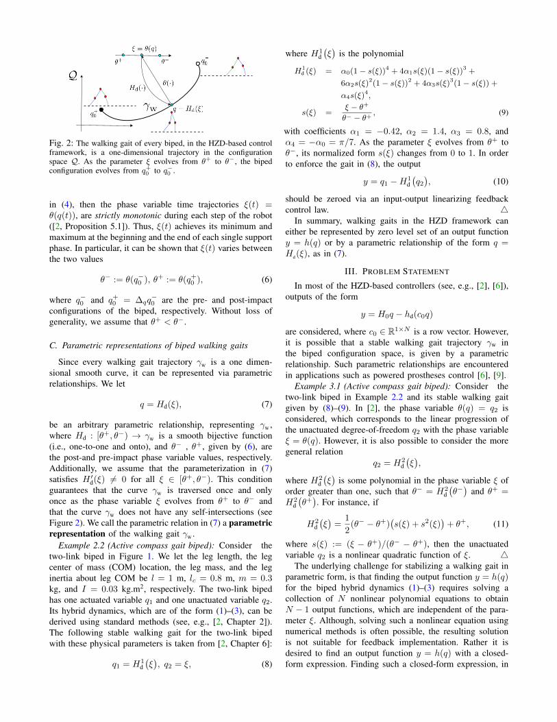
Fig. 2: The walking gait of every biped, in the HZD-based controlframework, is a one-dimensional trajectory in the configurationspace Q. As the parameter ξ evolves from θ+ to θ−, the bipedconfiguration evolves from q+0 to q−0 .

in (4), then the phase variable time trajectories ξ(t) =θ(q(t)), are strictly monotonic during each step of the robot([2, Proposition 5.1]). Thus, ξ(t) achieves its minimum andmaximum at the beginning and the end of each single supportphase. In particular, it can be shown that ξ(t) varies betweenthe two values

θ− := θ(q−0 ), θ+ := θ(q+0 ), (6)

where q−0 and q+0 = ∆qq−0 are the pre- and post-impact

configurations of the biped, respectively. Without loss ofgenerality, we assume that θ+ < θ−.

C. Parametric representations of biped walking gaits

Since every walking gait trajectory γW is a one dimen-sional smooth curve, it can be represented via parametricrelationships. We let

q = Hd(ξ), (7)

be an arbitrary parametric relationship, representing γW ,where Hd : [θ+, θ−) → γW is a smooth bijective function(i.e., one-to-one and onto), and θ− , θ+, given by (6), arethe post-and pre-impact phase variable values, respectively.Additionally, we assume that the parameterization in (7)satisfies H ′d(ξ) 6= 0 for all ξ ∈ [θ+, θ−). This conditionguarantees that the curve γW is traversed once and onlyonce as the phase variable ξ evolves from θ+ to θ− andthat the curve γW does not have any self-intersections (seeFigure 2). We call the parametric relation in (7) a parametricrepresentation of the walking gait γW .

Example 2.2 (Active compass gait biped): Consider thetwo-link biped in Figure 1. We let the leg length, the legcenter of mass (COM) location, the leg mass, and the leginertia about leg COM be l = 1 m, lc = 0.8 m, m = 0.3kg, and I = 0.03 kg.m2, respectively. The two-link bipedhas one actuated variable q1 and one unactuated variable q2.Its hybrid dynamics, which are of the form (1)–(3), can bederived using standard methods (see, e.g., [2, Chapter 2]).The following stable walking gait for the two-link bipedwith these physical parameters is taken from [2, Chapter 6]:

q1 = H1d

(ξ), q2 = ξ, (8)

where H1d

(ξ)

is the polynomial

H1d (ξ) = α0(1− s(ξ))4 + 4α1s(ξ)(1− s(ξ))3 +

6α2s(ξ)2(1− s(ξ))2 + 4α3s(ξ)

3(1− s(ξ)) +α4s(ξ)

4,

s(ξ) =ξ − θ+

θ− − θ+ , (9)

with coefficients α1 = −0.42, α2 = 1.4, α3 = 0.8, andα4 = −α0 = π/7. As the parameter ξ evolves from θ+ toθ−, its normalized form s(ξ) changes from 0 to 1. In orderto enforce the gait in (8), the output

y = q1 −H1d

(q2), (10)

should be zeroed via an input-output linearizing feedbackcontrol law. 4

In summary, walking gaits in the HZD framework caneither be represented by zero level set of an output functiony = h(q) or by a parametric relationship of the form q =Hd(ξ), as in (7).

III. PROBLEM STATEMENT

In most of the HZD-based controllers (see, e.g., [2], [6]),outputs of the form

y = H0q − hd(c0q)

are considered, where c0 ∈ R1×N is a row vector. However,it is possible that a stable walking gait trajectory γw inthe biped configuration space, is given by a parametricrelationship. Such parametric relationships are encounteredin applications such as powered prostheses control [6], [9].

Example 3.1 (Active compass gait biped): Consider thetwo-link biped in Example 2.2 and its stable walking gaitgiven by (8)–(9). In [2], the phase variable θ(q) = q2 isconsidered, which corresponds to the linear progression ofthe unactuated degree-of-freedom q2 with the phase variableξ = θ(q). However, it is also possible to consider the moregeneral relation

q2 = H2d

(ξ),

where H2d

(ξ)

is some polynomial in the phase variable ξ oforder greater than one, such that θ− = H2

d

(θ−)

and θ+ =H2

d

(θ+). For instance, if

H2d

(ξ)

=1

2(θ− − θ+)

(s(ξ) + s2(ξ)

)+ θ+, (11)

where s(ξ) := (ξ − θ+)/(θ− − θ+), then the unactuatedvariable q2 is a nonlinear quadratic function of ξ. 4

The underlying challenge for stabilizing a walking gait inparametric form, is that finding the output function y = h(q)for the biped hybrid dynamics (1)–(3) requires solving acollection of N nonlinear polynomial equations to obtainN − 1 output functions, which are independent of the para-meter ξ. Although, solving such a nonlinear equation usingnumerical methods is often possible, the resulting solutionis not suitable for feedback implementation. Rather it isdesired to find an output function y = h(q) with a closed-form expression. Finding such a closed-form expression, in

general, is impossible. In order to address this challenge, wesolve the following problem in this paper.

Parametric Gait Implicitization Problem. Consider

q = Hd(ξ), (12)

where Hd : [θ+, θ−) → Q is a smooth function, whoseimage represents the gait trajectory γW given by

γW = Hd

([θ+, θ−)

). (13)

Suppose that the components of the function Hd(·) are

Hid(ξ) =

ni∑k=0

bikξk, 1 ≤ i ≤ N, (14)

which are N polynomials of the real variable ξ such that thedegree of the ith polynomial is equal to ni. Find an outputfunction y = h(q), h(q) = [h1(q); · · · ;hN−1(q)], such thatit becomes zero on the gait trajectory γW . In other words,

h(Hd(ξ)

)= 0, (15)

for all ξ ∈ [θ+, θ−). Furthermore, determine necessary andsufficient conditions for the output y = h(q) to have vectorrelative degree {2, · · · , 2} for the biped dynamics. 4

Finding the output y = h(q), which implicitly representsthe walking gait trajectory γW through (15), enables usto enforce the given parametric representation in (12) byzeroing the output y = h(q). We call the process of bringinga parametric gait to its implicit form gait implicitization.

Solution Strategy. Our strategy for solving the parametricgait implicitization problem unfolds in two steps. In the firststep, presented in Section IV, we use a symbolic algebraic 2-by-2 elimination method, which is based on computing theresultant of polynomials, to eliminate the phase variable ξand find the implicit relationship between Hi

d(ξ) and Hjd (ξ),

i 6= j, in terms of the configuration variables qi and qj .Next, in Section V, we construct an output vector functiony = h(q) with N − 1 components such that it becomes zerowhenever q belongs to the walking gait γW . The generatedoutput implicitly represents the walking gait. We also find anecessary and sufficient condition for the constructed outputfunction y = h(q) to have well-defined vector relativedegree. 4

IV. IMPLICITIZATION OF TWO PARAMETRICPOLYNOMIALS

This section will establish the implicit relationship bet-ween any two given biped configuration variables that aregiven by parametric polynomials. We achieve this goal byremoving the phase variable using resultant of polynomials, atool which is frequently used in computer algebra. Necessarypreliminaries are provided in the Appendix.

Consider an arbitrary biped configuration represented bythe symbolic variable q and the walking gait curve γW in (13)with parametric polynomial representation (14). We definethe polynomials

P qii (ξ) := Hid(ξ)− qi, 1 ≤ i ≤ N. (16)

in the real variable ξ, where qi is the ith element of the vectorq. Indeed, bi0 − qi is the constant term of the polynomialP qii (ξ), i.e., the coefficient of ξ0 in (14). The parametricrelationship

P qii (ξ) = 0 =⇒ qi = Hid(ξ),

gives the trajectory of the ith joint variable during each wal-king step, as the parameter ξ varies in the interval [θ+, θ−).Now, we consider two arbitrary polynomials P qii (ξ) andPqjj (ξ), 1 ≤ i, j ≤ N , from the collection of polynomials

in (16). In order to remove the phase variable ξ and to findthe implicit relationship between the joint variables qi andqj during each step of the walking gait, we compute

hij(q) = Res(Hid(ξ)− qi, Hj

d (ξ)− qj), (17)

where Res(·, ·), defined by (A-2) in the Appendix, is theresultant of the polynomials P qii (ξ) and P qjj (ξ) in (16).

According to the definition of resultant in (A-2), the functi-ons hij(·) in (17) are independent of the phase variable ξ andonly depend on the coefficients of the polynomials P qii (ξ)and P qjj (ξ) in (16), i.e., bik, bjk, qi, and qj . The coefficientsbik, bjk are numerical, while qi, qj are symbolic variables.Computer algebra systems such as the MATLAB SymbolicMath Toolbox are capable of computing (17) symbolically(see Example 4.1). The resultant of the polynomials P qii (ξ)and P qjj (ξ) has the form

hij(q) =∑k,l

βklqki qlj ,

which is a symbolic bivariate polynomial (i.e., of two vari-ables), independent of the phase variable ξ.

Example 4.1 (Active compass gait biped): Consider thebiped gait walking trajectory in Example 3.1. Consider aparametric representation of the walking gait curve withq1 = H1

d (ξ) and q2 = H2d (ξ), where H1

d (·) and H2d (·)

are given by (9) and (11), respectively. Consider the twopolynomials P1(ξ) and P2(ξ), defined by (16), in the realvariable ξ. The variables q1 and q2, which are consideredto be the coefficients of ξ0, are symbolic. Computing theresultant of the two polynomials P1(·) and P2(·) wouldremove the parameter ξ and give us a bivariate polynomialin the joint variables q1 and q2. The implicit function h12(·)in (17) is

h12(q1, q2) = 0.003 + 0.27q21 + 1.49q1q22

−4.99q1q2 − 13.85q1 + 47.13q42

−0.36q32 − 1.41q22 − 0.68q2, (18)

which is a function of the symbolic variables q1 and q2, andindependent of the parameter ξ. 4

The functions hij(·) defined by (17) satisfy a fundamentalproperty at the biped configurations that belong to the wal-king gait curve (13), as stated in the following proposition.

Proposition 4.2: Consider the biped walking gait curveγW in (13) with parametric polynomial representation (14).Consider the collection of polynomials in (16), arbitrary

integers 1 ≤ i, j ≤ N , and the output function hij(q) givenby (17). Then, hij

(Hd(ξ)

)= 0, for all ξ ∈ [θ+, θ−).

Proof: Suppose that (qi, qj) = (Hid(ξ0), Hj

d (ξ0)), foran arbitrary ξ0 ∈ [θ+, θ−). Therefore, ξ0 is a common rootof the two polynomials P qii (ξ) and P qjj (ξ) defined by (16).By Part 2 of Lemma A1 in the Appendix, hij(Hd(ξ0)) = 0,because the two polynomials P qii and P

qjj have a common

root at ξ = ξ0.Proposition 4.2 states that the functions hij(q) in (17),

which are generated by taking the resultant of the parametricpolynomials Pi(ξ) and Pj(ξ), become zero whenever theconfiguration q belongs to the walking gait trajectory γW .Thus, the function hij(q) can be considered as an output forthe biped and driven to zero via feedback. Driving hij(q) tozero corresponds to making the desired relationship betweenqi and qj , which is prescribed by the given parametricrepresentation Hd(·), hold during each walking step.

V. SOLUTION TO THE GAIT IMPLICITIZATION PROBLEM

In this section we solve the parametric gait implicitizationproblem formulated in Section III. In particular, using thefunctions obtained in Section IV, we construct an outputvector function with N−1 components such that it becomeszero on the walking gait curve γW given by (13). Next, weprovide a necessary and sufficient condition for the generatedoutput function to have well-defined vector relative degree.

Given the walking gait curve γW in (13) with parametricpolynomial representation (14), we construct N−1 functions

hk(q) = hk,k+1(q), 1 ≤ k ≤ N − 1, (19)

where the functions hk,k+1(·) are defined by (17). Using thefunctions hk(q) in (19), we construct the output functiony = h(q), where

h(q) :=[h1(q); · · · ; hN−1(q)

], (20)

for the biped hybrid dynamics (1)–(3).The output function (20) has the property that it becomes

zero whenever q = Hd(ξ), due to Proposition 4.2. If thisoutput also satisfies a certain rank condition, then it canbe zeroed using an input-output feedback linearizing controllaw, as stated in the following proposition.

Proposition 5.1: Consider the gait curve γW in (13) withparametric polynomial representation (14). Consider the N−1 functions hk(q), 1 ≤ k ≤ N − 1, in (19) and the outputfunction y = h(q), where h(q) is given by (20). Supposethat B⊥D(Hd(ξ))H

′d(ξ) 6= 0 for all ξ ∈ [θ+, θ−], where

B⊥ = [01×(N−1) 1]. If

rank(∂h∂q

)= N − 1, (21)

for all q ∈ γW , then the output y = h(q) can be zeroed using

u =(∂h∂qD−1(q)B

)−1{v(y, y)− ∂

∂q

(∂h∂qq)q+

∂h

∂qD−1(q)[C(q, q)q +G(q)]

},

(22)

for the biped dynamics and v(y, y) is a high-gain PDfeedback or a continuous finite time stabilizer of the doubleintegrator y = v(y, y)2.

The proof is omitted for the sake of brevity.Remark 5.2: If the rank condition (21) is not satisfied for a

generated output y = h(q) associated with a given parametricrepresentation q = Hd(ξ) for some configurations q ∈ γW ,it is still possible to zero the output using the constraintaugmentation approach introduced in [2, Chapter 5]. 4

VI. SIMULATION STUDIES

Two-link walker. Consider the active two-link biped robotin Example 2.2 and the stable walking gait trajectory γW inFigure 1. The polynomial H1

d (ξ), given by (9), determinesthe desired evolution of the joint variable q1 during each step.The unactuated variable is q2, which varies between θ+ =−0.22 radians and θ− = 0.22 radians during each walkingstep. We consider the following three parameterizations forthe unactuated variable

H2ad

(ξ)

= ξ,

H2bd

(ξ)

=1

2(θ− − θ+)

(s(ξ) + s2(ξ)

)+ θ+,

H2cd

(ξ)

=1

3(θ− − θ+)

(s(ξ) + 2s3(ξ)

)+ θ+,

(23)

where s(ξ) is defined in (11). Also, H2ad (·), H2b

d (·), andH2c

d (·) correspond to a linear, a quadratic from (11), anda cubic parameterization of the unactuated variable q2 bythe parameter ξ, respectively.

In order to be able to enforce each of these parametricrepresentations, we need to find an output with closed-formexpression for each of the above parametric representations.For the linear parametric representation H2a

d (·), one caneasily set q2 = ξ and find its associated output ya = ha(q)given by (10). For the other two parametric representations,we use the methodology presented in the paper. First, weform the two polynomials P2b(·) and P2c(·) given by (16).Next, using (17) and (19), we obtain two different outputsy = hb(q) and y = hc(q), associated with the parametricrepresentations H2b

d (·) and H2cd (·). The function hb(q) is

given by (18). The function hc(q), whose expression hasbeen omitted for the sake of brevity, can also be computedusing any symbolic computer algebra system, similar toExample 4.1. All of these outputs satisfy the rank conditionin Theorem 5.1. Therefore, they can be zeroed via aninput-output feedback linearizing control input. The timeprofiles of the biped joints and their associated phase portraitsare demonstrated in Figures 3 and 4, respectively. In thisexample, different parameterizations of the unactuated degreeof freedom results in different biped walking speeds. 4

Three-link walker. Consider the three-link biped robotshown in Figure 1. We let the torso length, the leg length,the torso mass, the hip mass, and the leg mass to be l = 0.5m, r = 1.0 m, MT = 10 kg, MH = 15 kg, and m = 5 kg,respectively. The three-link biped has two actuated variables

2A possible choice for v(y, y) is the Bhat-Bernstein’s continuous timedouble integrator in [19], which is used on biped robots in [2].

0 1 2 3 4 5 6 7 8

t [sec]

-0.5

0

0.5

1

q1(t)[rad

]

0 1 2 3 4 5 6 7 8

t [sec]

-0.4

-0.2

0

0.2

0.4

q2(t)[rad

]

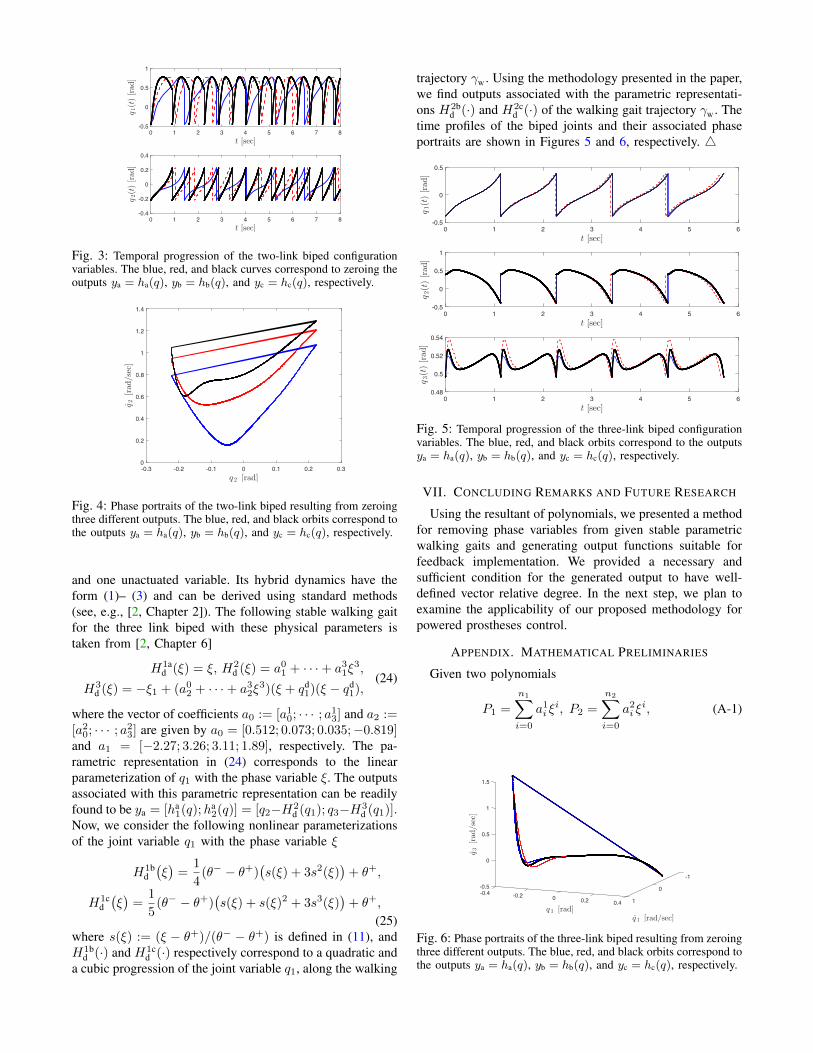
Fig. 3: Temporal progression of the two-link biped configurationvariables. The blue, red, and black curves correspond to zeroing theoutputs ya = ha(q), yb = hb(q), and yc = hc(q), respectively.

-0.3 -0.2 -0.1 0 0.1 0.2 0.3

q 2 [rad]

0

0.2

0.4

0.6

0.8

1

1.2

1.4

q2[rad

/sec]

Fig. 4: Phase portraits of the two-link biped resulting from zeroingthree different outputs. The blue, red, and black orbits correspond tothe outputs ya = ha(q), yb = hb(q), and yc = hc(q), respectively.

and one unactuated variable. Its hybrid dynamics have theform (1)– (3) and can be derived using standard methods(see, e.g., [2, Chapter 2]). The following stable walking gaitfor the three link biped with these physical parameters istaken from [2, Chapter 6]

H1ad (ξ) = ξ, H2

d (ξ) = a01 + · · ·+ a31ξ3,

H3d (ξ) = −ξ1 + (a02 + · · ·+ a32ξ

3)(ξ + qd1)(ξ − qd

1),(24)

where the vector of coefficients a0 := [a10; · · · ; a13] and a2 :=[a20; · · · ; a23] are given by a0 = [0.512; 0.073; 0.035;−0.819]and a1 = [−2.27; 3.26; 3.11; 1.89], respectively. The pa-rametric representation in (24) corresponds to the linearparameterization of q1 with the phase variable ξ. The outputsassociated with this parametric representation can be readilyfound to be ya = [ha

1(q);ha2(q)] = [q2−H2

d (q1); q3−H3d (q1)].

Now, we consider the following nonlinear parameterizationsof the joint variable q1 with the phase variable ξ

H1bd

(ξ)

=1

4(θ− − θ+)

(s(ξ) + 3s2(ξ)

)+ θ+,

H1cd

(ξ)

=1

5(θ− − θ+)

(s(ξ) + s(ξ)2 + 3s3(ξ)

)+ θ+,

(25)where s(ξ) := (ξ − θ+)/(θ− − θ+) is defined in (11), andH1b

d (·) and H1cd (·) respectively correspond to a quadratic and

a cubic progression of the joint variable q1, along the walking

trajectory γW . Using the methodology presented in the paper,we find outputs associated with the parametric representati-ons H2b

d (·) and H2cd (·) of the walking gait trajectory γW . The

time profiles of the biped joints and their associated phaseportraits are shown in Figures 5 and 6, respectively. 4

0 1 2 3 4 5 6

t [sec]

-0.5

0

0.5

q1(t)[rad]

0 1 2 3 4 5 6

t [sec]

-0.5

0

0.5

1

q2(t)[rad]

0 1 2 3 4 5 6

t [sec]

0.48

0.5

0.52

0.54

q3(t)[rad

]Fig. 5: Temporal progression of the three-link biped configurationvariables. The blue, red, and black orbits correspond to the outputsya = ha(q), yb = hb(q), and yc = hc(q), respectively.

VII. CONCLUDING REMARKS AND FUTURE RESEARCH

Using the resultant of polynomials, we presented a methodfor removing phase variables from given stable parametricwalking gaits and generating output functions suitable forfeedback implementation. We provided a necessary andsufficient condition for the generated output to have well-defined vector relative degree. In the next step, we plan toexamine the applicability of our proposed methodology forpowered prostheses control.

APPENDIX. MATHEMATICAL PRELIMINARIES

Given two polynomials

P1 =

n1∑i=0

a1i ξi, P2 =

n2∑i=0

a2i ξi, (A-1)

0.4 10.20

1.5

q 1 [rad]

-0.2

1

q3[rad/sec]

0.5

-0.4

0

-0.5 0

q 1 [rad/sec]

-1

Fig. 6: Phase portraits of the three-link biped resulting from zeroingthree different outputs. The blue, red, and black orbits correspond tothe outputs ya = ha(q), yb = hb(q), and yc = hc(q), respectively.

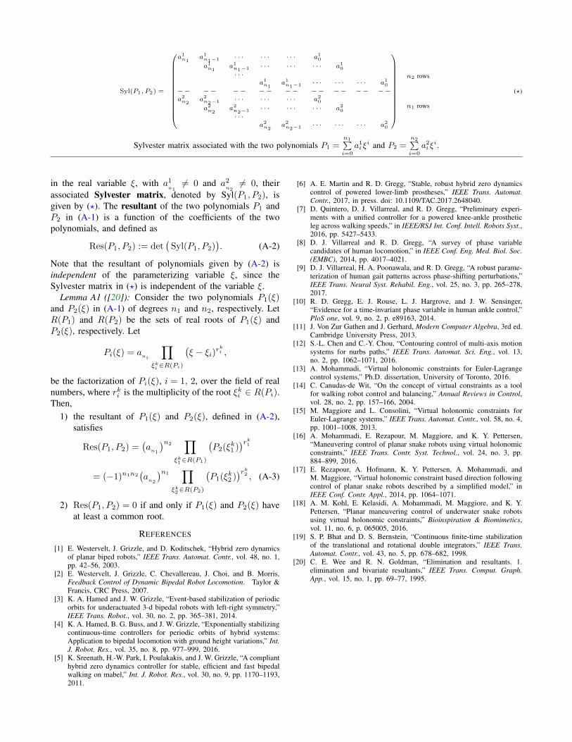
Syl(P1, P2) =

a1n1a1n1−1 · · · · · · · · · a10a1n1

a1n1−1 · · · · · · · · · a10· · ·

a1n1a1n1−1 · · · · · · · · · a10

−− −− −− −− −− −− −− −− −−a2n2

a2n2−1 · · · · · · · · · a20a2n2

a2n2−1 · · · · · · · · · a20· · ·

a2n2a2n2−1 · · · · · · · · · a20

n2 rows

n1 rows

(?)

Sylvester matrix associated with the two polynomials P1 =n1∑i=0

a1i ξi and P2 =

n2∑i=0

a2i ξi.

in the real variable ξ, with a1n16= 0 and a2

n26= 0, their

associated Sylvester matrix, denoted by Syl(P1, P2), isgiven by (?). The resultant of the two polynomials P1 andP2 in (A-1) is a function of the coefficients of the twopolynomials, and defined as

Res(P1, P2) := det(

Syl(P1, P2)). (A-2)

Note that the resultant of polynomials given by (A-2) isindependent of the parameterizing variable ξ, since theSylvester matrix in (?) is independent of the variable ξ.

Lemma A1 ([20]): Consider the two polynomials P1(ξ)and P2(ξ) in (A-1) of degrees n1 and n2, respectively. LetR(P1) and R(P2) be the sets of real roots of P1(ξ) andP2(ξ), respectively. Let

Pi(ξ) = ani

∏ξki ∈R(Pi)

(ξ − ξi)r

ki ,

be the factorization of Pi(ξ), i = 1, 2, over the field of realnumbers, where rki is the multiplicity of the root ξki ∈ R(Pi).Then,

1) the resultant of P1(ξ) and P2(ξ), defined in (A-2),satisfies

Res(P1, P2) =(an1

)n2∏

ξk1∈R(P1)

(P2(ξk1 )

)rk1= (−1)n1n2

(a

n2

)n1∏

ξk2∈R(P2)

(P1(ξk2 )

)rk2 , (A-3)

2) Res(P1, P2) = 0 if and only if P1(ξ) and P2(ξ) haveat least a common root.

REFERENCES

[1] E. Westervelt, J. Grizzle, and D. Koditschek, “Hybrid zero dynamicsof planar biped robots,” IEEE Trans. Automat. Contr., vol. 48, no. 1,pp. 42–56, 2003.

[2] E. Westervelt, J. Grizzle, C. Chevallereau, J. Choi, and B. Morris,Feedback Control of Dynamic Bipedal Robot Locomotion. Taylor &Francis, CRC Press, 2007.

[3] K. A. Hamed and J. W. Grizzle, “Event-based stabilization of periodicorbits for underactuated 3-d bipedal robots with left-right symmetry,”IEEE Trans. Robot., vol. 30, no. 2, pp. 365–381, 2014.

[4] K. A. Hamed, B. G. Buss, and J. W. Grizzle, “Exponentially stabilizingcontinuous-time controllers for periodic orbits of hybrid systems:Application to bipedal locomotion with ground height variations,” Int.J. Robot. Res., vol. 35, no. 8, pp. 977–999, 2016.

[5] K. Sreenath, H.-W. Park, I. Poulakakis, and J. W. Grizzle, “A complianthybrid zero dynamics controller for stable, efficient and fast bipedalwalking on mabel,” Int. J. Robot. Res., vol. 30, no. 9, pp. 1170–1193,2011.

[6] A. E. Martin and R. D. Gregg, “Stable, robust hybrid zero dynamicscontrol of powered lower-limb prostheses,” IEEE Trans. Automat.Contr., 2017, in press. doi: 10.1109/TAC.2017.2648040.

[7] D. Quintero, D. J. Villarreal, and R. D. Gregg, “Preliminary experi-ments with a unified controller for a powered knee-ankle prostheticleg across walking speeds,” in IEEE/RSJ Int. Conf. Intell. Robots Syst.,2016, pp. 5427–5433.

[8] D. J. Villarreal and R. D. Gregg, “A survey of phase variablecandidates of human locomotion,” in IEEE Conf. Eng. Med. Biol. Soc.(EMBC), 2014, pp. 4017–4021.

[9] D. J. Villarreal, H. A. Poonawala, and R. D. Gregg, “A robust parame-terization of human gait patterns across phase-shifting perturbations,”IEEE Trans. Neural Syst. Rehabil. Eng., vol. 25, no. 3, pp. 265–278,2017.

[10] R. D. Gregg, E. J. Rouse, L. J. Hargrove, and J. W. Sensinger,“Evidence for a time-invariant phase variable in human ankle control,”PloS one, vol. 9, no. 2, p. e89163, 2014.

[11] J. Von Zur Gathen and J. Gerhard, Modern Computer Algebra, 3rd ed.Cambridge University Press, 2013.

[12] S.-L. Chen and C.-Y. Chou, “Contouring control of multi-axis motionsystems for nurbs paths,” IEEE Trans. Automat. Sci. Eng., vol. 13,no. 2, pp. 1062–1071, 2016.

[13] A. Mohammadi, “Virtual holonomic constraints for Euler-Lagrangecontrol systems,” Ph.D. dissertation, University of Toronto, 2016.

[14] C. Canudas-de Wit, “On the concept of virtual constraints as a toolfor walking robot control and balancing,” Annual Reviews in Control,vol. 28, no. 2, pp. 157–166, 2004.

[15] M. Maggiore and L. Consolini, “Virtual holonomic constraints forEuler-Lagrange systems,” IEEE Trans. Automat. Contr., vol. 58, no. 4,pp. 1001–1008, 2013.

[16] A. Mohammadi, E. Rezapour, M. Maggiore, and K. Y. Pettersen,“Maneuvering control of planar snake robots using virtual holonomicconstraints,” IEEE Trans. Contr. Syst. Technol., vol. 24, no. 3, pp.884–899, 2016.

[17] E. Rezapour, A. Hofmann, K. Y. Pettersen, A. Mohammadi, andM. Maggiore, “Virtual holonomic constraint based direction followingcontrol of planar snake robots described by a simplified model,” inIEEE Conf. Contr. Appl., 2014, pp. 1064–1071.

[18] A. M. Kohl, E. Kelasidi, A. Mohammadi, M. Maggiore, and K. Y.Pettersen, “Planar maneuvering control of underwater snake robotsusing virtual holonomic constraints,” Bioinspiration & Biomimetics,vol. 11, no. 6, p. 065005, 2016.

[19] S. P. Bhat and D. S. Bernstein, “Continuous finite-time stabilizationof the translational and rotational double integrators,” IEEE Trans.Automat. Contr., vol. 43, no. 5, pp. 678–682, 1998.

[20] C. E. Wee and R. N. Goldman, “Elimination and resultants. 1.elimination and bivariate resultants,” IEEE Trans. Comput. Graph.App., vol. 15, no. 1, pp. 69–77, 1995.