Reliability in sealing of canister for spent nuclear · PDF fileReliability in sealing of...

Reliability in sealing of canister for spent nuclear fuel

Ulf Ronneteg, Bodycote Materials Testing AB

Lars Cederqvist, Håkan Rydén

Svensk Kärnbränslehantering AB

Tomas Öberg, Tomas Öberg Konsult AB

Christina Müller, BAM – Federal Institute for Materials

Research and Testing, Berlin

June 2006

R-06-26

R-0

6-2

6R

eliability in

sealing

of can

ister for sp

ent n

uclear fu

el

Svensk Kärnbränslehantering ABSwedish Nuclear Fueland Waste Management CoBox 5864SE-102 40 Stockholm Sweden Tel 08-459 84 00 +46 8 459 84 00Fax 08-661 57 19 +46 8 661 57 19

CM

Gru

ppen

AB

, Bro

mm

a, 2

006

Reliability in sealing of canister for spent nuclear fuel

Ulf Ronneteg, Bodycote Materials Testing AB

Lars Cederqvist, Håkan Rydén

Svensk Kärnbränslehantering AB

Tomas Öberg, Tomas Öberg Konsult AB

Christina Müller, BAM – Federal Institute for Materials

Research and Testing, Berlin

June 2006

ISSN 1402-3091

SKB Rapport R-06-26

A pdf version of this document can be downloaded from www.skb.se

�

Summary

The reliability of the system for sealing the canister and inspecting the weld that has been developed for the Encapsulation plant was investigated. In the investigation the occurrence of discontinuities that can be formed in the welds was determined both qualitatively and quantitatively. The probability that these discontinuities can be detected by nondestructive testing (NDT) was also studied.

The friction stir welding (FSW) process was verified in several steps. The variables in the welding process that determine weld quality were identified during the development work. In order to establish the limits within which they can be allowed to vary, a screening experi-ment was performed where the different process settings were tested according to a given design. In the next step the optimal process setting was determined by means of a response surface experiment, whereby the sensitivity of the process to different variable changes was studied. Based on the optimal process setting, the process window was defined, i.e. the limits within which the welding variables must lie in order for the process to produce the desired result. Finally, the process was evaluated during a demonstration series of 20 sealing welds which were carried out under production-like conditions.

Conditions for the formation of discontinuities in welding were investigated. The investiga-tions show that the occurrence of discontinuities is dependent on the welding variables. Discontinuities that can arise were classified and described with respect to characteristics, occurrence, cause and preventive measures.

To ensure that testing of the welds has been done with sufficient reliability, the probability of detection (POD) of discontinuities by NDT and the accuracy of size determination by NDT were determined.

In the evaluation of the demonstration series, which comprised 20 welds, a statistical method based on the generalized extreme value distribution was fitted to the size estimate of the indications obtained with NDT. The predicted maximum discontinuity size in connec-tion with the welding of 4,500 canisters at the present stage of development of the process was conservatively determined to be less than one centimetre. All factors considered, the predicted minimum copper coverage for a 5 cm thick canister is 4 cm.

Acceptance criteria for permitted settings in the welding process in a future sealing system are proposed, as is the use of statistical process control based on nondestructive testing as an independent inspection system. Furthermore, principles for handling of process noncon-formances are presented.

�

Contents

1 Background 7

2 Purposeofthereport 9

3 Frictionstirwelding(FSW) 113.1 Description of the welding process 113.2 Description of the welding system 13

4 Verificationoftheweldingprocess 154.1 Screening 154.2 Optimization 164.3 Process window 214.4 Alternative evaluation of response surface experiment 23

5 Nondestructivetesting(NDT) 255.1 Description of NDT systems 25

5.1.1 System for digital radiography 255.1.2 System for phased array ultrasonic testing 26

5.2 Description of NDT processes 275.2.1 Principles of digital radiography 275.2.2 Principles of phased array ultrasonic testing 29

6 Descriptionofpossiblediscontinuities 316.1 Discontinuities detectable by NDT 326.2 Discontinuities not detectable by NDT, supplementary examinations 36

6.2.1 Completed examinations 366.2.2 Description of discontinuities 37

7 NDTreliability 417.1 Background 417.2 Strategy 417.3 Practical procedure 437.4 Results 43

7.4.1 Probability of Detection, POD 437.4.2 Accuracy in size estimation 47

8 Demonstrationseries 538.1 Evaluation of process and system 538.2 Evaluation of demonstration series with NDT 568.3 Examination of occurrence of discontinuities not detected by NDT 57

8.3.1 Examination by destructive testing 578.3.2 Examination by microfocus X-rays 57

8.4 Mechanisms that cause formation of discontinuities 588.5 Demonstration of preventive measures against discontinuities 58

9 Predictionoffutureproductionquality 599.1 Statistical methods 599.2 Results 609.3 Prediction error and measurement uncertainty 639.4 Process window in future production 63

�

10 Acceptancecriteriafordiscontinuities 6510.1 Strategy 6510.2 Acceptance criteria 65

10.2.1 The first acceptance criterion 6510.2.2 The second acceptance criterion 6610.2.3 Requirements for testability 68

10.3 Application of the proposed criteria 6910.4 Comments 69

11 MTOfactors 71

12 QualificationofprocesseswithinSealingSubsystem 7312.1 Welding 7312.2 Nondestructive testing 7312.3 Acceptance criteria 74

13 Conclusions 75

14 Futurelineofaction 7714.1 Process FSW 7714.2 Process NDT 7814.3 Other processes in production system for canisters 78

15 References 79

16 Abbreviations 81

Appendix1 NDT Reliability 83

�

1 Background

This report comprises a basis for SKB’s safety assessment SR-Can. SR-Can analyzes the long-term safety of a KBS-3 type final repository, where copper canisters with a cast iron insert are filled with spent nuclear fuel and deposited at a depth of approximately 500 m in granitic rock surrounded by bentonite clay. SR-Can is based on preliminary site data from SKB’s ongoing investigations of candidate sites for a final repository for spent nuclear fuel in Forsmark and Laxemar. When final data from the site investigations are available, a renewed evaluation of long-term safety will be done in the safety assessment SR-Site. SR-Site will comprise a basis for SKB’s application for a permit to build a final repository. The canister’s initial copper coverage is a crucial item of information for the assessments of the long-term safety of the repository, and the quality of the canister’s welded joints, which is the subject of this report, is a cornerstone of this issue.

In its review statement on RD&D 2001 /SKI 2002/, SKI stated: “A sufficiently large number of canisters must have been fabricated, sealed and inspected and found to comply with the requirements of the long-term safety assessment”. The strategy that has been applied to obtain data for the assessment of the long-term safety of the final repository entails determination of the reliability of the processes included in the future production system. The production system is divided into three subsystems, see Figure 1-1: • Copper Subsystem, used to produce the copper shell and includes fabrication and inspec-

tion of copper components for canisters that are delivered to the encapsulation plant.• Insert Subsystem, used to produce the cast iron insert and includes fabrication and

inspection of the insert and its components.• Sealing Subsystem, used for sealing of the canister and includes welding, machining and

inspection of the weld.

This report concerns the reliability of the Sealing Subsystem. Similar investigations for the Copper and Insert subsystems are planned prior to SR-Site.

The first theoretical discussions of the programme were presented in the planning report SR-Can /SKB 2003/. The final strategy and the methods intended to be used were presented in 2004 /Müller and Öberg 2004/. The timetable for the programme was presented in SKB’s plan of action /SKB 2004a/. The main points in the programme have been:1. Verification and demonstration of the welding processes electron beam welding (EBW)

and friction stir welding (FSW).– Investigation of the robustness of the processes with respect to permissible variations

in the process variables.– Verification that the processes can be carried out on full scale by sealing of a

complete canister.– Demonstration of serial production capacity and achieved weld quality by welding

20 lids for each welding process.2. Investigation of reliability in nondestructive testing (NDT) of the sealing process.3. Statistical analysis and prediction of future production quality.

�

Up until March 2005, SKB worked in parallel on the development of two welding methods at the Canister Laboratory: friction stir welding (FSW) and electron beam welding (EBW). For the continued work leading up to a permit application for the encapsulation plant, May 2005 was deemed to be a suitable time to choose a reference method for sealing. The criteria for choice of reference method are described in greater detail in /SKB 2006a/. Now that FSW has been chosen as the reference method, the in-depth analysis work has been concentrated on FSW and the results are only reported for FSW.

Figure 1-1. Production system for canisters.

Suppliers Canister factory Encapsulation plant

Steel cassette

Fabrication

Insert

Casting

Steel lid

Fabrication

Copper ingot

Fabrication

Copper components

Extrusion of the tube

Forging of lid and bottom

Insert Subsystem

Copper Subsystem

Insert

Finish machining

Dimensional inspection

Nondestructive testing

Copper components

Finish machining

Dimensional inspection


Bottom weld

Welding

Finish machining


Ass

embl

y of

can

iste

r

Sealing Subsystem

Welding

Finish machining


Sealing weld

�

2 Purposeofthereport

The purpose of the report is to give an account of: • The reliability of the welding process.• The reliability of the NDT process developed in parallel with the welding process.• The predicted reliability of the Sealing Subsystem in a future production process. • The programme for verification and demonstration of the sealing process that was

mentioned in SKB’s plan of action /SKB 2004a/.

The outline of the report is as follows:

Chapter 3. Description of the FSW system at the Canister Laboratory and the sealing proc-ess that has been developed.

Chapter 4. Account of how verification of the welding method has been done. The chapter describes the investigations of the various process settings, how they interact and the size of the process window.

Chapter 5. Description of the processes and systems for NDT that have been developed to detect discontinuities in the weld metal.

Chapter 6. Account of discontinuities that can occur in welds made by FSW.

Chapter 7. Account of the reliability of the NDT processes.

Chapter 8. Description of the demonstration series of 20 welds. An account is given of operating experience and the quality of the welds.

Chapter 9. Description of the prediction of the future process outcome of welding of 4,500 canisters.

Chapter 10. Presentation of proposed acceptance criteria for Sealing Subsystem.

Chapter 11. Discusses in general terms factors with respect to Man-Technology-Organization (MTO).

Chapter 12. Describes how this study can be used in future qualification of the welding and NDT processes.

Chapter 13. Conclusions.

Chapter 14. Future line of action.

Chapter 15. References.

Chapter 16. Abbreviations.

11

3 Frictionstirwelding(FSW)

Friction stir welding (FSW) is a type of friction welding that was invented in 1991 at The Welding Institute in Cambridge, England. FSW is a thermo mechanical solid-state process, i.e. not a fusion welding method. This means that the problems encountered in fusion welding – such as unfavourable grain structure, grain growth and segregation phenomena – can be avoided. The resulting microstructure in FSW of copper thus resembles the micro-structure resulting from hot forming of the copper components in the canister. The process and system are described in general terms in this chapter, while a more detailed description is provided in /Cederqvist 2005/.

3.1 DescriptionoftheweldingprocessA rotating tool consisting of a tapered probe and shoulder, see Figure 3-1, are plunged into the weld metal. The function of the probe is to heat up the weld metal by means of friction and, by virtue of its shape and rotation, force the metal to flow around it and create a weld. The function of the shoulder is to heat up the metal by means of friction and prevent it from being squeezed out of the joint. Figure 3-2 shows when the tool is advanced along the joint and forms a weld.

One reason for the rapidly increasing use of FSW in industry is that the method has few welding variables. This means that the welding process is simple to control. The welding tool rotates at a specific number of revolutions per minute and moves along the joint at a constant speed. The position of the tool shoulder in relation to the canister surface is then controlled with a specific downward force. In most cases the tool is also angled in relation to the work-piece so that the tool shoulder “surfs” on the surface.

Besides the adjustable variables (called welding factors), the resulting variables (called welding responses) are measured. These factors are the depth of the shoulder in the weld metal, the tool temperature, the torque of the spindle motor and the force on the tool in the direction of travel.

Figure 3-1. The welding tool. Figure 3-2. Schematic drawing of the FSW process.

12

There is a clear relationship between welding factors and welding responses, for example the product of the rotation speed and the torque of the spindle motor is equal to the heat input and thereby affects the temperature of the tool. These relatively elementary relation-ships make the process simple to interpret, develop and control.

The welding machine that is used in the Canister Laboratory has cooling of both the lid clamps and the tool holder. However the cooling has a secondary influence on the process. The purpose of cooling is to protect the machine against high temperatures and reduce wear on the spindle motor and the tool holder.

A weld cycle can be divided into several sequences, which are shown in Figure 3-3. First a start hole is drilled 75 mm above the joint line which the rotating tool is then plunged into so that the copper is heated. When the tool temperature has reached a set value, the weld-ing speed is accelerated to a constant value as a function of the tool temperature. After the acceleration sequence is finished and the tool temperature has stabilized, i.e. reached the “steady-state”, the tool is moved down to the joint line. After a full revolution at the joint line, the tool is moved up 75 mm above the joint line, where the welding cycle is terminated and the tool is withdrawn resulting in the unavoidable exit hole. Both the acceleration sequence and the exit hole are then machined off when the lid is given its final dimensions.

The acceleration sequence is important since it affects flash formation and the risk of discontinuities during the downward sequence. The other sequences, nos. 2–5 in Figure 3-3, can be merged into the “steady-state” sequence where all variables remain at a relatively constant value.

After the canister is positioned in the machine, it takes about an hour to seal the canister, including clamping of canister and lid (5 minutes), drilling of start hole (5 minutes) and welding (50 minutes). The time required for the process in the encapsulation plant is estimated to be equivalent. Experience from the Canister Laboratory shows that several canisters can be sealed in a day.

Figure 3-3. Sequences in a weld cycle: 1. acceleration sequence, 2. downward sequence, 3. joint line sequence, 4. overlap sequence, and 5. parking sequence.

12

3 4

5

Flash

3

1�

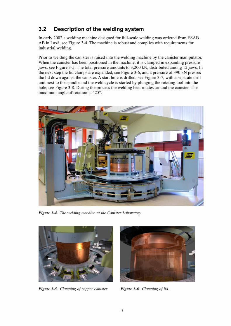
3.2 DescriptionoftheweldingsystemIn early 2002 a welding machine designed for full-scale welding was ordered from ESAB AB in Laxå, see Figure 3-4. The machine is robust and complies with requirements for industrial welding.

Prior to welding the canister is raised into the welding machine by the canister manipulator. When the canister has been positioned in the machine, it is clamped in expanding pressure jaws, see Figure 3-5. The total pressure amounts to 3,200 kN, distributed among 12 jaws. In the next step the lid clamps are expanded, see Figure 3-6, and a pressure of 390 kN presses the lid down against the canister. A start hole is drilled, see Figure 3-7, with a separate drill unit next to the spindle and the weld cycle is started by plunging the rotating tool into the hole, see Figure 3-8. During the process the welding heat rotates around the canister. The maximum angle of rotation is 425°.

Figure 3-4. The welding machine at the Canister Laboratory.

Figure 3-5. Clamping of copper canister. Figure 3-6. Clamping of lid.

14

The tool (see Figure 3-1) is an important component in FSW. The tool must withstand a high process temperature, as well as the high forces to which it is subjected during welding. A sealing weld takes about 50 minutes and is four metres long.

A nickel-base superalloy (Nimonic 105) is used as the material in the tool probe. Nickel-base alloys have good high-temperature properties with good wear resistance and sufficient strength for canister sealing. The tool shoulder is made of a tungsten alloy (Denismet) with suitable thermal and mechanical properties for the process. The probe is changed after each sealing weld while the shoulder can be used for several welds.

The software that monitors the welding process logs all variables every tenth of a second, i.e. with a frequency of 10 Hz. During the welding process, selected variables are displayed numerically and graphically to the welding operator. Two video cameras also show the tool from the rear and the front. With the exception of the acceleration sequence where the welding speed increases to a constant value as a function of the welding temperature, all regulation of the welding process is performed manually by the welding operator (at present by changes in spindle speed and/or axial force). As described in the future line of action in Chapter 14, the development of a fully automated welding process is an important milestone prior to qualification of the welding system and welding procedure.

Since the tool temperature has proved to be very important, two separate and independent measurements of this variable are currently made. Since the installation of the welding system, a thermocouple has been placed in the tool probe to measure the temperature during the weld cycle, which is the value reported as the tool temperature in this report. An infrared camera was also installed in the autumn of 2005 to measure the temperature of the tool shoulder. This has proved to be an excellent complement to the thermocouple in the tool /SKB 2006a/.

Figure 3-7. Drilling of start hole. Figure 3-8. Tool in start hole.

1�

4 Verificationoftheweldingprocess

The FSW process was evaluated by means of a statistical methodology (see Figure 4-1) aimed at optimizing process settings and determining the process window /Müller and Öberg 2004, Box and Draper 1987, Box et al. 1978/. In order to verify the welding process, the welding variables that determine weld quality were identified /Öberg 2006a/. Then the limits within which these variables (welding factors) could be allowed to vary were deter-mined by a screening experiment. In the next step a so-called response surface experiment was conducted to determine the optimal process setting /Öberg 2006a/ and then the process window was defined. Finally, the optimized process was evaluated by a series of 20 sealing welds under production-like conditions.

4.1 ScreeningAs described previously in Section 3.1, there are four welding factors that can be varied and four welding responses. Experience from previous welding trials, shows that the welding responces that are most important for the weld quality are the depth of the shoulder in the canister and the temperature of the tool. Suitable values for shoulder depth and tool temperature are 0.6 mm and 855°C.

The desired value for tool temperature applies during the joint line sequence, while the desired value for shoulder depth only applies during the acceleration sequence, the down-ward sequence and approximately ten degrees of joint line welding. After these sequences, this variable cannot be used to control the process since it was not possible to obtain an accurate value of the shoulder depth at that point in time. The reason for this is a combina-tion of the fact that the canister is not perfectly centred in the welding system, deflections in the welding system and thermal expansion of the canister.

During three lid welds consisting of 22 separate weld cycles, a wide range of values was tried for each welding factor (Table 4-1) and the effect of this variation on the welding responses (Table 4-2) was studied /Cederqvist 2005/.

Figure 4-1. Verification of the welding process.

Verification of the process

Screening Optimization Process window

Demonstration series

1�

Table4-1. Weldingfactors.

Variable Unit Testedrange

Welding speed (WS) mm/min 60–130Spindle speed (SS) rpm 350–500

Axial force (FZ) kN 70–105Tool angle ° 2–4

Table4-2. Weldingresponses.

Variable Unit Testedrange

Shoulder depth mm 0–4Tool temp °C 690–945

Spindle torque Nm 750–1,200Traverse force kN 25–70

The screening experiments showed that the tool angle did not notably affect the weld quality within the tested range. As a result, spindle speed, welding speed and axial force were chosen in the optimization study.

4.2 OptimizationThe response surface method was used to optimize the process. Three welding factors were included in the trial series: welding speed (WS), spindle speed (SS) and axial force (FZ). The choice of variation range is shown in Table 4-3. High, medium and low level for each factor is indicated by 1, 0 and –1.

Each test entailed welding for 45°, permitting eight tests in one revolution. The number of tests in the trial series was 16, and they were performed on two sealing welds. The chosen experimental plan, a response surface experiment according to Box-Behnken, permits estimation of an empirical polynomial model with linear interaction and quadratic terms /Box and Draper 1987/. The experimental plan is shown in Table 4-4. The response surface models (polynomial) were fitted to the measurement data by multiple linear regression. The model terms (interactions) that were not significant were removed, and the final models contained three linear and three quadratic terms.

Table4-3. Levelsforthedifferentweldingfactorsintheresponsesurfaceexperiment.

Level/factor –1 0 1

WS: (mm/min) 100 80 60SS: (rpm) 360 400 440

FZ: (kN) 86 89 92

1�

The values of the shoulder depth and the tool temperature at the end of the test (see Table 4-5) were used to evaluate the experiments and choose optimal settings for further operation. The desired values for shoulder depth and tool temperature were 0.6 mm and 855°C, respectively. Since the tests were at most 45°, the value of the shoulder depth is considered accurate since the centring and thermal expansion of the canister only affected the value marginally.

Table4-4. Experimentalplanforevaluationoftheweldingprocess.

Test Weld Segment Weldingspeed(WS)

Spindlespeed(SS)

Weldingforce(FZ)

1 1 0–45° 0 0 02 1 45–90° 1 0 –1

3 1 90–135° 0 –1 14 1 135–180° 0 0 05 1 180–225° 1 0 16 1 225–270° –1 0 17 1 270–315° 0 0 08 1 315–360° 0 –1 –19 2 0–45° –1 –1 010 2 45–90° 0 1 –111 2 90–135° 1 –1 012 2 135–180° –1 1 013 2 180–225° 0 1 114 2 225–270° 0 0 015 2 270–315° –1 0 –116 2 315–360° 1 1 0

Table4-5. ResultsofresponsesurfaceexperimentwithFSW.

Test Shoulderdepth(mm)

Tooltemperature(°C)

1 1.0 8202 0.8 885

3** 0.4 7504** 1.0 7605** 1.6 9206** 0.9 7607 0.5 7908 0.4 7709** 0.8 77010** 2.2 91011 1.1 82012** 2.8 92013** 2.4 93014*/** (2.4) (880)15 0.5 73016** 2.2 920

* = Test 14 was excluded because a poor start hole may have affected the result. **= To avoid the risk of damaging the welding system, these tests were terminated before 45° was reached.

1�

The two regression models that were fitted to these data were both statistically significant. The variance contribution from each welding factor is shown in Tables 4-6 and 4-71.

The importance of the different welding factors within the investigated domain is shown directly by the P values. Welding speed (WS) only influences weld temperature, while spindle speed (SS) is important in both cases. The evaluation can also be done by examining the disturbance plots, where the effect of changing one welding factor at a time is shown, see Figures 4-2 and 4-3. The effects can be examined independently of each other, since there is no interaction in the investigated process window.

Table4-6. Analysisofvarianceforaresponsesurfacemodelwithregardtoshoulderdepth.

Source s.s. d.f. m.s. F P

Model 8.08 6 1.35 13.19 0.0009WS 0.061 1 0.061 0.60 0.4609

SS 5.95 1 5.95 58.30 < 0.0001FZ 0.24 1 0.24 2.40 0.1599WS^2 0.22 1 0.22 2.19 0.1775SS^2 1.54 1 1.54 15.09 0.0046FZ^2 0.062 1 0.062 0.60 0.4596Residuals 0.82 8 0.10Model error 0.65 6 0.11 1.30 0.4958Experimental error 0.17 2 0.083Total 8.90 14

Table4-7. Analysisofvarianceforaresponsesurfacemodelwithregardtotooltemperature.

Source s.s. d.f. m.s. F P

Model 66,173 6 11,029 6.92 0.0078WS 16,653 1 16,653 10.45 0.0120

SS 40,612 1 40,612 25.48 0.0010

FZ 5,28.1 1 528.1 0.33 0.5807WS^2 2,424 1 2425 1.52 0.2524SS^2 6,474. 1 6475 4.06 0.0786FZ^2 243.8 1 243.8 0.15 0.7059Residuals 12,750 8 1,594Model error 10,950 6 1,825 2.03 0.3666Experimental error 1,800 2 900.0Total 78,923 14

1 Acronyms in the analysis of variance tables: s.s. = sum of squares, d.f. = degrees of freedom, m.s. = mean squares (s.s./d.f.), F = test quantity (ratio of ss for model to residuals, or model error to experimental error) and P = probability in relation to the F distribution.

1�

Figure 4-2. Influence on shoulder depth between high and low level for the relevant welding factor.

Figure 4-3. Influence on tool temperature between high and low level for the relevant welding factor.

WS

SS

FZ

0.4

0.8

1.2

1.6

2

2.4

-1 -0.5 0 0.5 1

Deviation from reference point

Shou

lder

dep

th (m

m)

WS

SS

FZ

730

780

830

880

930

-1 -0.5 0 0.5 1

Deviation from reference point

Tool

tem

pera

ture

(°C

)

20

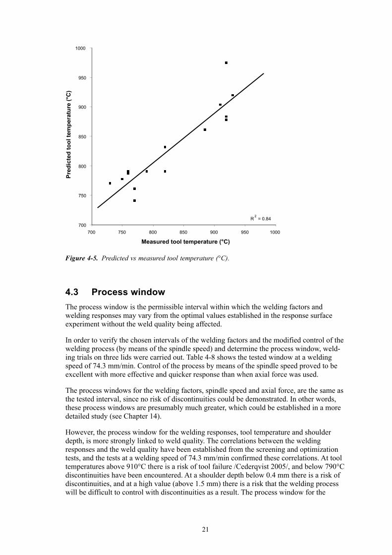
The agreement between model predictions and measurement results is shown in Figures 4-4 and 4-5.

The conclusions of the response surface experiment are:• In the early welding trials, weld quality and the welding responses were controlled by

means of small changes (0.5 kN) in axial force. However, the response surface experi-ment shows that spindle speed is the most important factor, which makes it more suitable for controlling the process.

• Welding speed was the next most important welding factor. Its influence on tool temperature was similar to that of spindle speed. This factor should, however, be kept constant to not increase the risk of forming discontinuities.

• The variations in axial force were of no importance within the studied range, which meant that it should be used as a secondary control factor.

A suitable operating setting entails a compromise between the two optimization criteria (the previously called desired values for shoulder depth and tool temperature). Based on the response surface experiment, the optimal values for the welding factors were found to be: welding speed 74.3 mm/min, spindle speed 410 rpm and axial force 87 kN. According to the response surface models, this process setting will result in a shoulder depth of 0.96 (± 0.36) mm and a tool temperature of 824 (± 45)°C (standard errors within parentheses).

Figure 4-4. Predicted vs measured shoulder depth (mm).

R2 = 0.91

0

0.5

1

1.5

2

2.5

3

0 0.5 1 1.5 2 2.5 3

Measured shoulder depth (mm)

Pred

icte

d sh

ould

er d

epth

(mm

)

21

4.3 ProcesswindowThe process window is the permissible interval within which the welding factors and welding responses may vary from the optimal values established in the response surface experiment without the weld quality being affected.

In order to verify the chosen intervals of the welding factors and the modified control of the welding process (by means of the spindle speed) and determine the process window, weld-ing trials on three lids were carried out. Table 4-8 shows the tested window at a welding speed of 74.3 mm/min. Control of the process by means of the spindle speed proved to be excellent with more effective and quicker response than when axial force was used.

The process windows for the welding factors, spindle speed and axial force, are the same as the tested interval, since no risk of discontinuities could be demonstrated. In other words, these process windows are presumably much greater, which could be established in a more detailed study (see Chapter 14).

However, the process window for the welding responses, tool temperature and shoulder depth, is more strongly linked to weld quality. The correlations between the welding responses and the weld quality have been established from the screening and optimization tests, and the tests at a welding speed of 74.3 mm/min confirmed these correlations. At tool temperatures above 910°C there is a risk of tool failure /Cederqvist 2005/, and below 790°C discontinuities have been encountered. At a shoulder depth below 0.4 mm there is a risk of discontinuities, and at a high value (above 1.5 mm) there is a risk that the welding process will be difficult to control with discontinuities as a result. The process window for the

Figure 4-5. Predicted vs measured tool temperature (°C).

R2 = 0.84

700

750

800

850

900

950

1000

700 750 800 850 900 950 1000

Measured tool temperature (°C)

Pred

icte

d to

ol te

mpe

ratu

re (°

C)

22

welding responses is illustrated graphically in Figure 4-6 and contains the results from the response surface experiment at the end of the acceleration sequence plus the results from the response surface models for the chosen process setting.

As Table 4-8 shows, the tested process window for tool temperature is 790–910°C. To put this window in perspective it can be compared with welding data from the first lid weld after the demonstration series. Figure 4-7 shows welding data from the “steady-state” sequence, i.e. sequence 2–5 in Figure 3-3 in a sealing weld, which is equivalent to a weld-ing distance of 390° or 45 minutes. The tool temperature lies between 835 and 860°C, i.e. ± 12°C compared with the process window of ± 60°C.

Table4-8. Influenceoftheweldingfactorsandtheweldingresponsesontheprocess.

Factor/response Window Athighvalue Atlowvalue

Spindle speed (rpm) 350–450 Risk of high tool temperature –Axial force (kN) 78–98 Risk of high tool temperature Risk of discontinuities

Tool temperature (°C) 790–910 Risk of tool failure Risk of discontinuitiesShoulder depth (mm) 0.4–1.5 Risk of discontinuities Risk of discontinuities

Figure 4-6. Process window for welding responses including data from response surface experiment (red points refer to welds with discontinuities).

0.0

0.5

1.0

1.5

2.0

2.5

3.0

3.5

750 790 830 870 910 950

Tool temperature (°C)

Shou

lder

dep

th (m

m)

Responce surface experiment Chosen process setting

Not possible to machine canister clean from tool shoulder footprint

Risk of discontinuities

Ris

k of

dis

cont

inui

ties

Ris

k of

tool

failu

re


2�

4.4 AlternativeevaluationofresponsesurfaceexperimentA number of tests in the response surface experiment did not reach steady-state, see Table 4-5, and had to be terminated before 45° had been welded to not risk damage (due to high forces and/or high temperature) to the welding system. In order to verify that this did not affect the analysis, an alternative analysis was subsequently carried out on the welding tests in Table 4-4 /Öberg 2006b/. In this analysis, welding variables in an earlier stage of the weld cycle (at the start of the downward sequence) were used, since no tests had been terminated at that point. The values for shoulder depth and tool temperature at this important stage of the weld cycle are shown in Table 4-9.

The conclusions from the alternative analysis of the response surface experiment are:• The two regression models that were fitted to these measurement data are statistically

significant.• The relationships between welding factors and welding variables are essentially similar

to the original analysis with spindle speed as a suitable welding factor to control the process. However, these models exhibit a slightly poorer fit to the measurement data, especially the model for shoulder depth, which is however still statistically significant.

• The welding speed is no longer a significant factor in the response surface model for tool temperature. This result is understandable, since it is an early stage of the weld cycle where welding speed has not had time to influence the process.

• The optimal values for the welding factors that were determined in Section 4.2 give a similar outcome, with a shoulder depth of 0.81 (± 0.45) mm and a tool temperature of 833 (± 32)°C, for the alternative response surface analysis (standard errors within parentheses). The similar results show that the original analysis was not markedly affected by the early terminated tests.

Figure 4-7. Welding data from lid weld. * value on right-hand y axis.

24

Table4-9. ResultsofresponsesurfaceexperimentwithFSW.

Test Shoulderdepth(mm) Tooltemperature(°C)

1 0.9 8542 0.7 810

3 0.5 7684 1.0 8025 1.5 8756 0.9 8577 0.5 7988 0.4 7989 0.8 77910 1.7 91911 1.0 83012 2.8 90013 1.2 91914* (1.5) (834)15 0.5 79216 1.9 906

* = Test 14 was excluded because a poor start hole may have affected the result.

2�

5 Nondestructivetesting(NDT)

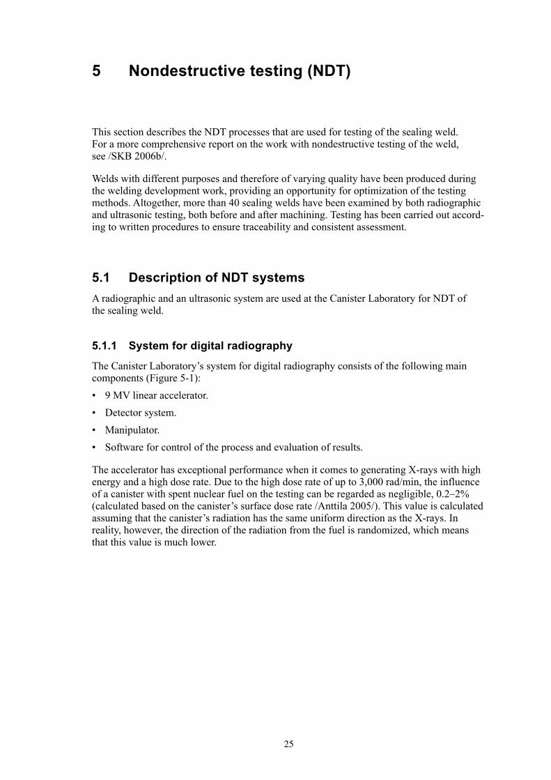
This section describes the NDT processes that are used for testing of the sealing weld. For a more comprehensive report on the work with nondestructive testing of the weld, see /SKB 2006b/.

Welds with different purposes and therefore of varying quality have been produced during the welding development work, providing an opportunity for optimization of the testing methods. Altogether, more than 40 sealing welds have been examined by both radiographic and ultrasonic testing, both before and after machining. Testing has been carried out accord-ing to written procedures to ensure traceability and consistent assessment.

5.1 DescriptionofNDTsystemsA radiographic and an ultrasonic system are used at the Canister Laboratory for NDT of the sealing weld.

5.1.1 Systemfordigitalradiography

The Canister Laboratory’s system for digital radiography consists of the following main components (Figure 5-1):• 9 MV linear accelerator.• Detector system.• Manipulator.• Software for control of the process and evaluation of results.

The accelerator has exceptional performance when it comes to generating X-rays with high energy and a high dose rate. Due to the high dose rate of up to 3,000 rad/min, the influence of a canister with spent nuclear fuel on the testing can be regarded as negligible, 0.2–2% (calculated based on the canister’s surface dose rate /Anttila 2005/). This value is calculated assuming that the canister’s radiation has the same uniform direction as the X-rays. In reality, however, the direction of the radiation from the fuel is randomized, which means that this value is much lower.

2�

5.1.2 Systemforphasedarrayultrasonictesting

In ultrasonic testing based on phased array technology, an ultrasound sensor with a large number of probe elements is used. The technology permits electronic focusing and control of the sound beam.

The Canister Laboratory’s system for phased array ultrasonic testing consists of the follow-ing main components (Figure 5-2):• TD Focus-Scan MKI ultrasonic inspection unit.• A large number of planar probes with 32–128 elements within a frequency range of

2.7–10 MHz.• Software for data acquisition and evaluation.• Manipulator with system for fixing of probes.

Figure 5-1. X-ray machine for testing of the copper canister’s sealing weld.

2�

5.2 DescriptionofNDTprocessesIn order to ensure good and repeatable quality in nondestructive testing of the canister’s lid weld, procedures have been established for testing and evaluation. They include software settings, mechanical settings, reference normals and evaluation criteria.

5.2.1 Principlesofdigitalradiography

The main principle is that the canister rotates while the accelerator pulses X-rays through the weld with an incident angle of 35° (see Figure 5-3 below). The transmitted radiation is detected by a linear detector (100 mm high) positioned perpendicular to the beam with a vertical resolution (channel width) of 0.4 mm. This same resolution is achieved in the vertical direction by a collimator (vertical gap) that focuses the beam, and the X-ray image is built up with every 0.4 mm rotation of the canister (see Figure 5-4 below). The effect of potential discontinuities in the weld is a decrease of absorption of the x-ray leading to darker area on the x-ray image. The result is then evaluated using criteria based on the geometry of the canister in relation to the radiation direction and the system’s signal/noise ratio.

The numbers in the figure above show where the indications in the radiograph at the right are located in the weld. The vertical axis represents the welding direction with the start point at the top. To compensate for the large variations in copper thickness in the beam path, a mean value calibration is performed.

Figure 5-2. Ultrasonic inspection unit for testing of the copper canister’s sealing weld.

2�

Figure 5-3. Schematic illustration of radiographic testing of weld.

Figure 5-4. Radiograph.

Detector

Weld

X-rays

2�

5.2.2 Principlesofphasedarrayultrasonictesting

The testing principle is that the canister rotates while an ultrasound probe electronically scans the sound beam in the radial direction (see Figure 5-5). The probe consists of 80 piezoelectric elements that are individually excited by high voltage electrical pulses in order to generate an ultrasonic wave with a centre frequency of 5 MHz in the material. The excitation of each element is electronically triggered allowing a dynamic control over the shape and position of the sound beam. In order to ensure coupling of the sound waves inside the canister, a thin water film is used as a coupling agent. To ensure that testing covers the whole weld with respect to possible discontinuities (Chapter 6), the sound is focused elec-tronically on different depths and with varying angles in the radial direction. Discontinuities reflect part of sound beam back to the array. The results are presented in the form of a two-dimensional image (C-scan), see Figure 5-6, composed of the maximal amplitude for each index point. The results are evaluated by locating indications with an amplitude above a given threshold value and determining their size by the half value method /International Institute of Welding 1987/.

Figure 5-5. Principle of ultrasonic testing of FSW.

�0

Figure 5-6. Ultrasound of FSW, A-scan at top, C-scan in middle and B-scan at bottom.

�1

6 Descriptionofpossiblediscontinuities

This chapter describes the discontinuities that have been shown possible to generate with FSW in 5 cm thick copper. A more detailed description of the possible discontinuities in the weld is provided in the report /SKB 2006a/.

The discontinuities described below occur in many cases only under extreme conditions, while others are more common. A number of approaches have been used to catalogue the possible discontinuities:• Indications from NDT of welds performed at the Canister Laboratory have been

examined, as well as welds from the development work at TWI. The indications have been verified by metallographic examination.

• Examinations of areas where the welding process has been outside the process window. Pieces have been cut out in selected areas for further study by radiographic examination, and in certain cases also by metallography.

• Randomly selected samples have been examined by microfocus X-ray inspection, followed in some cases by metallographic examinations.

• Furthermore, a number of metallographic examinations by independent laboratories have provided information on above all tiny discontinuities or other anomalies not detected by NDT.

Of the discontinuities described, only some occur in connection with welding with variables inside or close to the process window. They are also described in Chapter 8.

There is at present no specific classification system for discontinuities for FSW. The possible discontinuities have therefore been classified according to the system deemed to be the closest, which applies to geometric imperfections in metallic materials associated with pressure welding /Swedish Standards Institute 2003/.

�2

Table6-1. Classificationofdiscontinuities.

ReferenceSS-EN-ISO6520(ISO6520-2:2001)

Designationandexplanation Illustration

P 403 InsufficientfusionInsufficient fusion in the joint.

P 2013 LocalizedporosityEvenly distributed group of pores.

P 2016 WormholeA tubular cavity in the weld metal, generally grouped in clusters and distributed in a herringbone formation.

P 303 OxideinclusionThin metallic oxide inclusions in the weld (isolated or clustered).

P 304 MetallicinclusionA particle of foreign metal trapped in the weld metal.

6.1 DiscontinuitiesdetectablebyNDTIn the trials with FSW at the Canister Laboratory, two types of discontinuities in particular have been indicated: joint line hooking, JLH (P 4013) and wormholes (P 2016), see Figure 6-1.

��

Joint line hooking (insufficient of fusion) ISO 6520-2:2001 P. 403

Joint line hooking, JLH, (see Figure 6-2) can occur in the internal part of the weld as a consequence of bending of the vertical joint between the tube and the lid during welding. The detectability of this type of discontinuity is very good with ultrasound (see Figure 6-3), while it cannot be detected by radiography.

Description: The joint between the inside of the tube and the lid is bent towards the tool shoulder due to the flow of material around the tool probe.

Size: Up to 5.5 mm extent in radial direction has been noted. Normally, JLH has a tangen-tial extent of one or two decimetres. However, in extreme cases these discontinuities may extend along the entire weld revolution.

Location: In the weld root.

Characteristics: Dense crack-like discontinuity with extent in radial direction with a gap of <10 µM, angle radial/axial < 20°. Good surface finish.

Occurrence: At the overlap sequence (see Figure 3-3) in all lid welds.

Importanceforpropertiesintheweldmetal: Reduces the corrosion barrier.

Cause: The flow of material causes the vertical joint line to be pulled out in the horizontal direction. The size of the JLH is linked to the penetration of the tool probe.

Figure 6-1. Location of discontinuities in welds.

Joint line hooking

Wormholes

�4

Prevention: JLH can be minimized (see also Section 8.5) by reducing the flow of material in the area by reducing the depth of penetration of the tool probe or by changing the flow direction of the material by changing the welding or rotation direction.

Testingmethod: Ultrasonic testing from the top of the lid with the sound direction in the range ± 20°.

Figure 6-2. Macrospecimen of JLH.

Figure 6-3. Indications of JLH obtained in ultrasonic testing.

��

Wormhole ISO 6520-2:2001 P. 2016

Wormholes (see Figure 6-4) can occur in the outer part of the weld as a consequence of welding variables outside the process window. The detectability of this type of discontinuity is good with ultrasound (see Figures 6-5 and 6-6) but it can only be detected by radiography in the extreme case when it forms a volumetric discontinuity.

Description: Near-surface discontinuity that arises on the advancing side of the tool /Cederqvist 2005/, which can also break the surface during the acceleration sequence.

Size: Up to 10 mm extent in radial direction has been noted when welding variables are outside the process window. The extent in the tangential direction is less than 10 mm, although clusters of discontinuities can have a much greater tangential extent.

Location: Has been detected from the surface down to a depth of 10 mm.

Characteristics: Irregular shape with uneven surfaces. Usually consists of clusters with dense discontinuities in the tangential direction with a primary extent in the radial/axial direction. In some cases when the welding variables are far from the process window, wormholes may merge into volumetric discontinuities.

Occurrence: Large discontinuities were found early in the development of the welding process, but only small discontinuities (< 3 mm) have been indicated in more recent welds.

Importanceforpropertiesintheweldmetal: Reduces the corrosion barrier.

Cause: Welding variables, low shoulder depth and/or low tool temperature, outside the process window.

Prevention: Welding variables inside the process window.

Figure 6-4. Macrospecimen of volumetric wormhole.

��

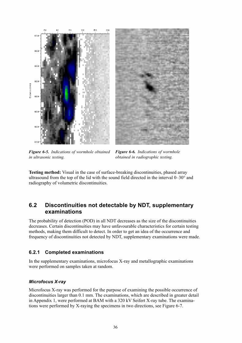
Figure 6-5. Indications of wormhole obtained in ultrasonic testing.

Figure 6-6. Indications of wormhole obtained in radiographic testing.

Testingmethod: Visual in the case of surface-breaking discontinuities, phased array ultrasound from the top of the lid with the sound field directed in the interval 0–30° and radiography of volumetric discontinuities.

6.2 DiscontinuitiesnotdetectablebyNDT,supplementaryexaminations

The probability of detection (POD) in all NDT decreases as the size of the discontinuities decreases. Certain discontinuities may have unfavourable characteristics for certain testing methods, making them difficult to detect. In order to get an idea of the occurrence and frequency of discontinuities not detected by NDT, supplementary examinations were made.

6.2.1 Completedexaminations

In the supplementary examinations, microfocus X-ray and metallographic examinations were performed on samples taken at random.

Microfocus X-ray

Microfocus X-ray was performed for the purpose of examining the possible occurrence of discontinuities larger than 0.1 mm. The examinations, which are described in greater detail in Appendix 1, were performed at BAM with a 320 kV Seifert X-ray tube. The examina-tions were performed by X-raying the specimens in two directions, see Figure 6-7.

��

In the examinations, specimens were randomly cut out from all welds in the demonstration series. These specimens were then machined to bars (20×20×80) mm) suitable for examina-tion in the radiography system.

The results of these examinations are presented in Chapter 8.

Metallographic examinations

As a complement to the microfocus X-ray examinations, various metallographic examina-tions were also performed. One round of examinations included thorough inspection of eight drill cores taken randomly from welds. The drill cores had a diameter of 40 mm and the examination was conducted by slicing up the material in 0.5 mm increments and exam-ining the section surfaces visually. A total of 800 sections were studied. Furthermore, some 20-odd macrospecimens were taken out for more careful examination under a microscope. These examinations were supplemented by SEM examinations with EDS and refined microscopy.

The results of these examinations are presented in Chapter 8.

6.2.2 Descriptionofdiscontinuities

Three types of small discontinuities were found in FSW welds. • Pores and clustered porosities.• Oxide inclusions.• Metallic inclusions.

Figure 6-7. Setup for microfocus X-ray.

1000

mm

Weld surface

0º

Film D2

Wel

d su

rfac

e

90º

Film D2

��

Clustered porosity ISO 6520-2:2001 P. 2013

Description: Single pores or pore strings.

Size: Strings up to 9 mm long were observed. The pores are around 0.1–0.5 mm in size.

Location: Found in all parts of the weld.

Characteristics: See Figure 6-8.

Occurrence: When welding was done inside the process window only single small pores were observed in certain welds.

Importanceforpropertiesintheweldmetal: When welding is done inside the process window they have little effect on the effective corrosion barrier.

Cause: Clustered porosities arise when one or more welding variables are outside the process window. Single pores can arise at random.

Prevention: Make sure that welding is done inside the process window. Near-surface clustered porosities are often machined off when the lid is machined to its final dimensions.

Examinationmethod: Can only be detected by metallographic examinations.

Figure 6-8. Clustered porosity in overlap zone on lid weld 35.

��

Oxide inclusions

Description: Copper oxide, see Figure 6-9.

Size:Oxides of length < 300 μm were detected.

Location:Normally occur near the surface in an area that is machined off.

Occurrence:Found in all examined lid welds, usually in the overlap sequence.

Importanceforpropertiesintheweldmetal: Very little effect on the effective corrosion barrier.

Cause:If welding is done in an atmosphere with oxygen, copper oxidizes rapidly and the oxide is stirred into the weld metal.

Prevention: Tests are planned where welding will be done in shielding gas.

Examinationmethod: Can only be detected by metallographic examinations.

Figure 6-9. Cluster of oxidized particles in the overlap zone on lid weld 36.

40

Metallic inclusions

Description:Traces of tool material in the weld metal, se Figure 6-10.

Size:Particles of length < 300 μm were detected.

Location:Usually near the surface but distributed throughout weld zone.

Occurrence:In all lid welds.

Importanceforpropertiesintheweldmetal: Due to the small size of the particles, they are not expected to affect the corrosion barrier.

Cause: Tool wear.

Prevention:Requires further study, see Section 8.5.

Examinationmethod: Can be detected by high-sensitive radiography on cut-out specimens or by chemical analysis of the weld metal as elevated concentration of foreign metals.

Figure 6-10. Traces of foreign material (W) near-surface in unmachined lid weld 20.

41

7 NDTreliability

A project was started in 2003 at BAM (Bundesanstalt für Materialforschung- und Prüfung) entitled “NDT Reliability” in order to determine the reliability of the NDT processes. The results of the project are outlined in this chapter. A more detailed description is provided in Appendix 1 and in the project’s final report /Müller et al. 2006/.

7.1 BackgroundAn initial study to determine the ability of the NDT processes to detect and determine the size of discontinuities was conducted in 2001 /Ronneteg and Moberg 2003/. The study included 43 discontinuities that had been indicated in electron beam welds where size estimated by ultrasound and radiography was compared with size estimated by metallo-graphic examinations. The study showed good correlation between size estimated by NDT and measured size.

The “NDT Reliability” project at BAM included evaluation of NDT of welds made by both FSW and EBW for the purpose of determining POD (Probability of Detection), and preci-sion in estimation of the size of discontinuities.

7.2 StrategyBy “NDT reliability” is meant the ability to detect and determine the size of discontinuities and to estimate the risk of false calls.

In order to determine the reliability of NDT processes, they can be divided into three parts (see Figure 7-1), where each part influences the reliability of the process:• The intrinsic physical capability of the method to detect relevant discontinuities for the

process (IC).• Technical application factors that influence the testing (AP).• Effects of human factors (HF).

The goal in this project has been to determine the capability of the NDT process to detect and determine the size of discontinuities, with a focus on the physical variables. Other application factors and human factors will be studied at a later stage when the technical solutions have been finalized. The goal is that these factors will be minimized in the design of processes and systems.

The method that BAM used to determine the Probability of Detection (POD) of the NDT processes uses the ratio between signal strength â from the detection system and the size of the discontinuity a, see Figure 7-2. The method is described in MIL-HDBK 1823 /US Department of Defence 1999/ and was developed for the USA’s military space industry.

Figure 7-3 shows a POD curve where POD is plotted against the size of the discontinuity. The value a90/95 is used as a measure of POD. The indexation (90/95) indicates that 90% of the discontinuities with size a will be detected within a confidence interval of 95%, i.e. the uncertainty in determination of the POD curve.

42

Figure 7-1. NDT reliability.

Figure 7-2. General description of methodology for determination of POD.

For automated thresholding systems a forecast of the POD is possible from the statistics of the response signals

aâ

a â POD

defect size signal magnitude probability of detection

experiments or modelling

calculations withlog-normal-distribution

(or other statistical model)

response

typical POD

POD

a

100 %

log a

log â

linear or more general relationship


aâ

a â POD





response

typical POD

POD

a

100 %

log a

log â



aâ

aâ

a â POD





typical POD

POD

a

100 %

log a

log â POD

a

100 %

log a

log â

response

4�

7.3 PracticalprocedureIn order to obtain suitable specimens, welds were performed where as the processes were intentionally disturbed. Examples of disturbances in the welds are contamination and damage to joint surfaces and deviation from normal process variables. The purpose was to generate a large number of different discontinuities that could arise in the processes. Furthermore, supplementary material from other welds was used to provide a large enough body of statistics for the analysis.

The welds were examined by NDT according to the Canister Laboratory’s procedures for radiographic and ultrasonic testing. Specimens and examination results from NDT were delivered to BAM, where the specimens were examined by different reference methods: immersion ultrasonic testing, HECT (High Energy Computed Tomography) and µ-CT (Microfocus Computed Tomography). Supplementary evaluation was also done at the Canister Laboratory. Finally, metallographic examinations were also carried out to verify the occurrence, shape and extent of the discontinuities.

7.4 ResultsThe results of the reliability study include the capability of the NDT process to detect (POD) and determine the size of different types of discontinuities.

7.4.1 ProbabilityofDetection,POD

In the case of wormhole-type discontinuities, it has not been possible to obtain a direct relationship between signal size and radial size of the discontinuities. In the case of radiography, first a value of a90/95 for penetrated thickness was determined with HECT (Figure 7-4). Then this value was correlated to the actual size of the discontinuities

Figure 7-3. Example of POD curve where 95% lower confidence bound crosses 90% POD.

0 2 4 6 8 10 12

0.0

0.2

0.4

0.6

0.8

1.0

Radial size (destr.), mm

POD

POD

lower 95% conf. bound

POD = 0.9

a 90/9

5 = 3

.2

44

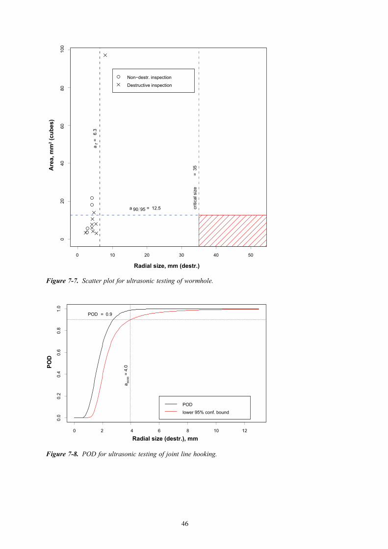
(Figure 7-5), giving a value of 4 mm for ar. Further studies /Müller et al. 2006/ show however that optimized threshold levels from radiographic evaluation can improve these values. It should also be noted that the discontinuities used in this study were generated in welds with weld variables outside the process window and that they are thereby volumetric. In the case of ultrasound, first a value of a90/95 was determined for the reflected area of the discontinuities in immersion testing (Figure 7-6). Then this value was correlated to the actual size of the discontinuities (Figure 7-7), giving a value of 6.3 mm for ar.

In the case of discontinuities of the JLH type, a direct relationship between signal strength and the radial size of the discontinuities was used as a consequence of the fact that the tangential extent is much greater than the sound field in this direction. These specimens exhibit a POD a90/95 of 4.0 mm, see Figure 7-8.

The results are compiled in Table 7-1, while a more detailed discussion is presented in Appendix 1.

Figure 7-4. POD for radiographic testing of wormhole.

0 1 2 3 4

0.0

0.2

0.4

0.6

0.8

1.0

Penetrated size (BAM-CT) [mm]

POD

PODlower 95% conf. bound

POD = 0.9

a 90/9

5 = 2

.60

4�

Figure 7-5. Scatter plot for radiographic testing of wormhole.

Figure 7-6. POD for ultrasonic testing of wormhole.

10 20 30 0

0

2

4

6

810

Radial size, mm

Pene

trat

ed s

ize

(BA

M−C

T), m

mDestr. inspectionNon−destr. inspectiony=x

a90 95= 2.6

criti

cal s

ize

=35

ar=

4

40

0 5 10 15 20 25

0.0

0.2

0.4

0.6

0.8

1.0

Area, mm2 (cubes)

POD

POD = 0.9

a 90/9

5 = 1

2.5

4�

Figure 7-7. Scatter plot for ultrasonic testing of wormhole.

Figure 7-8. POD for ultrasonic testing of joint line hooking.

0 10 20 30 40 50

2040

6080

100

0

Radial size, mm (destr.)

Are

a, m

m2 (

cube

s)

a 90 95 = 12.5 criti

cal s

ize

=35

ar=

6.3

Non−destr. inspection

Destructive inspection

0 2 4 6 8 10 12

0.0

0.2

0.4

0.6

0.8

1.0


POD

POD


POD = 0.9

a 90/9

5 = 4

.0

4�

Table7-1. PODresultsforFSW.

a90/95UT(mm) a90/95RT(mm)Wormhole 6.3 mm 4.0 mm

JLH 4.0 mm

7.4.2 Accuracyinsizeestimation

The measurement error in nondestructive testing can be estimated with a reference method (destructive test). Input data, size estimated by NDT and size estimated by destructive testing, as well as measurement error (the difference), are presented in Tables 7-2, 7-3 and 7-4. The distribution of the measurement errors is shown by frequency histograms in Figures 7-9, 7-10 and 7-11.

Table7-2. Measurementerrorwithultrasonictesting,acomparisonwithdestructivetestingwithregardtoindicationsofJLH.

Test Size,UT(mm) Size,reference(mm)

Measurementerror(mm)

1 4.0 3.3 0.72 4.0 5.4 –1.4

3 4.0 3.3 0.74 4.5 4.5 –0.05 4.0 4.8 –0.86 3.0 2.6 0.47 4.0 3.3 0.78 3.5 4.2 –0.79 4.0 4.1 –0.110 4.5 4.2 0.311 4.0 3.5 0.512 3.5 3.0 0.513 3.5 2.4 1.114 3.0 1.8 1.215 3.0 1.7 1.316 2.5 2.0 0.517 4.0 4.7 –0.718 3.0 3.9 –0.919 4.0 1.5 2.520 3.0 1.4 1.621 4.0 2.8 1.222 4.0 4.1 –0.123 4.0 2.7 1.3

4�

Table7-3. Measurementerrorwithultrasonictesting,acomparisonwithdestructivetestingwithregardtoindicationsofwormholes.



1 5.0 5.3 –0.32 6.5 7.9 –1.4

3 2.5 2.7 –0.24 2.0 4.1 –2.15 4.0 2.8 1.26 2.0 4.1 –2.17 3.0 4.3 –1.38 2.5 4.2 –1.79 2.5 3.1 –0.610 2.0 2.2 –0.211 4.5 5.2 –0.712 5.0 4.6 0.4

Table7-4. Measurementerrorwithradiographictesting,acomparisonwithdestructivetestingwithregardtoindicationsofwormholes.



1 5.5 5.3 0.22 13.8 7.9 5.9

3 1.8 2.7 –0.94 5.0 4.1 0.95 1.7 4.1 –2.46 2.4 4.3 –1.97 3.0 4.2 –1.28 3.0 3.1 –0.19 5.3 5.2 0.110 4.4 4.6 –0.2

4�

Figure 7-9. Histogram of measurement error for UT of JLH.

0

1

2

3

4

5

6

-1.5--1.0 -1.0--0.5 -0.5--0 0-0.5 0.5-1.0 1.0-1.5 1.5-2.0 2.0-2.5

Measurement error (mm)

Num

ber

Figure 7-10. Histogram of measurement error for UT of wormholes.

0

1

2

3

4

5

6

-3.0--2.0 -2.0--1.0 -1.0-0 0-1.0 1.0-2.0


Num

ber

�0

Estimated uncertainty interval

As regards JLH-type discontinuities, the results show that the mean value for the measure-ment errors is 0.426 with a standard deviation of 0.929. A two-sided 95% confidence interval for the mean value calculated with re-sampling (Efron’s percentile method) varies from 0.056 to 0.796 mm /Efron and Tibshirani 1998/. The maximum measurement error is an overestimation of the defect size by 2.5 mm (test 19 in Table 7-2 above).

The measurement error for JLH-type discontinuities is size-dependent and exhibits a clear relationship with the defect size indicated from the reference method, Figure 7-12. The size of small defects (< 3 mm) is overestimated by NDT and larger defects (> 4 mm) are underestimated. A similar relationship does not exist with the measured defect size, which means the NDT results cannot be simply corrected to eliminate the systematic error.

As regards wormhole-type discontinuities measured by ultrasound, the results show that the mean value for the measurement errors is –0.750 with a standard deviation of 1.010. A two-sided 95% confidence interval for the mean value calculated with resampling varies from –1.128 to –0.192 mm. The maximum measured measurement error is an under-estimation of the size by 2.1 mm (tests 4 and 6 in Table 7-3 above).

As regards wormhole-type discontinuities measured with radiography, the results show that the mean value for the measurement errors is 0.040 with a standard deviation of 2.293. A two-sided 95% confidence interval for the mean value calculated with resampling varies from –1.090 to 1.550 mm. The maximum measured measurement error is an overestimation of the size by 5.9 mm (test 2 in Table 7-4 above).

Figure 7-11. Histogram of measurement errors for RT of wormholes.

0

1

2

3

4

-3.0-2.0 -2.0--1.0 -1.0-0 0-1.0 1.0-2.0 2.0-3.0 3.0-4.0 4.0-5.0 5.0-6.0


Num

ber

�1

Figure 7-12. Measurement error with ultrasound as a function of defect size determined by destructive testing (mm).

y = -0,7213x + 2,7237

R2 = 0,743

-2

-1

0

1

2

3

1 2 3 4 5 6

Defect size (mm)

Mea

sure

men

t err

or (m

m)

��

8 Demonstrationseries

As mentioned in Chapter 1, the purpose of the demonstration series was to show the weld quality that can be achieved under production-like forms and to show that the welding process and the welding system can be operated in serial production. The demonstration programme was carried out in late 2004 and early 2005 and consisted of 20 lid welds.

8.1 EvaluationofprocessandsystemAll 20 welds in the demonstration series were carried out under production-like forms. No tests of the system or the process needed to be carried out in addition to the lid welds. In other words, the demonstration series could be carried out without interruption, which shows that process and system have high reliability and availability.

Table 8-1 shows mean, minimum and maximum values as well as standard deviations for the welding factors during a complete revolution (360° in the X direction) of joint line welding for all lid welds in the demonstration series. Equivalent results for the welding responses, tool temperature and shoulder depth, are presented in Table 8-2. However, shoulder depth was only checked at the start of the downward sequence. The parking sequence (Figure 3-3) is begun by a manual command, which leads to just over 360° of joint line welding. The part of the weld that is overlapped is thus not included in the analysis of the process window. Figure 8-1 shows the tool temperature over these 360° of joint line welding for all 20 welds.

Table8-1. Weldingfactorsindemonstrationseries.

WeldID Spindlespeed(SS) Weldingforce(FZ)Mean Min Max Stdev Mean Min Max Stdev

22 405 370 436 12.9 84.9 80.0 91.3 2.3

23 403 370 437 15.2 84.7 80.6 92.6 2.224 393 360 442 17.0 84.1 79.5 90.8 2.225 409 385 442 14.4 84.9 80.5 94.3 2.426 410 390 436 10.6 85.0 81.0 91.3 2.227 397 375 432 11.4 84.7 80.7 93.7 2.328 384 355 442 14.0 84.0 79.7 91.2 2.329 405 377 419 9.0 84.5 79.8 94.5 2.430 395 357 434 15.0 84.7 80.8 91.5 2.231 396 357 424 14.3 85.5 80.9 93.3 2.432 398 377 429 11.6 86.2 80.3 94.5 2.633 399 367 429 13.0 85.8 81.0 93.1 2.434 392 372 444 15.9 86.9 81.6 94.8 2.535 398 367 443 11.4 86.8 81.2 93.6 2.536 407 387 434 8.9 86.3 81.0 93.2 2.537 385 362 429 10.5 88.3 82.6 93.7 2.538 400 377 428 11.0 88.0 82.4 95.5 2.539 379 357 398 7.4 84.4 79.4 90.0 2.240 379 352 414 15.3 87.3 82.3 93.0 2.441 388 357 444 15.6 87.8 83.0 94.3 2.4Mean 396 369 432 12.7 85.7 80.9 93.0 2.4

�4

Table8-2. Weldingresponsesindemonstrationseries.

WeldID Tooltemperature(TT) Shoulderdepth(PZ)Mean Min Max St.dev

22 861 836 879 7.0 0.823 859 825 881 11.8 1.324 859 828 874 5.3 1.125 856 831 868 5.9 1.126 856 844 873 4.9 0.827 857 831 876 6.0 1.128 854 826 899 7.0 1.229 854 835 878 5.8 1.230 855 829 874 6.3 0.831 855 839 871 4.9 1.032 854 829 867 5.7 1.133 854 839 866 4.9 1.034 853 817 864 7.1 1.235 854 828 869 5.2 1.336 851 821 865 7.6 1.037 853 838 873 5.1 0.738 851 824 867 6.3 1.039 853 835 885 5.8 1.140 854 836 872 4.7 1.041 850 798 877 10.6 1.6Mean 854 829 874 6.4 1.1

Figure 8-1. Tool temperature during 360° of joint line welding with weld ID.

790

810

830

850

870

890

910

0 45 90 135 180 225 270 315 360

Position in X direction (degrees)

Tool

tem

pera

ture

(deg

rees

Cel

sius

)

22 23 24 25 26 27 28 29 30 31

32 33 34 35 36 37 38 39 40 41

��

Figure 8-2 shows how the position of the different lid welds compared with the process window at the start of the downward sequence (Figure 3-3).

The demonstration series has shown that the process that has been developed and optimized is robust and repeatable. The process could be run within the tested process window (see Table 4-8 in Chapter 4.3) with good margin. It was, however, noted that one weld (ID 41) had a shoulder depth of 1.6 mm (process window 0.4–1.5 mm) when the downward sequence started. The process was adjusted to correct this, which caused the tool temperature to fall to 778°C (process window 790–910°C) for a brief period. The area where this happened was, however, within the overlap zone and was thereby automatically rewelded, this time with variables inside the process window (Table 8-2 and Figure 8-1).

Figure 8-2. Process window for the weld responses with data from the demonstration series.

0.0

0.5

1.0

1.5

2.0

2.5

3.0

3.5

750 790 830 870 910 950

Tool temperature (ºC)

Shou

lder

dep

th (m

m)

Not possible to machine canister clean from tool shoulder footprint


Ris

k of

dis

cont

inui

ties

Ris

k of

tool

failu

re


��

8.2 EvaluationofdemonstrationserieswithNDTAll 20 welds in the demonstration series were examined by nondestructive testing both before and after machining. The testing before machining was used to verify that correct settings had been used in the welding process. After machining, all welds were examined by both phased array ultrasonic testing and digital radiography according to the Canister Laboratory’s procedures.

No volumetric discontinuities were detected by digital radiography. A total of 54 disconti-nuities were indicated by ultrasonic testing. Joint line hooking was indicated in all welds with a radial extent in the range 2–5 mm, see distribution in Figure 8-3. Verifying destruc-tive testing was performed in order to determine the true radial size of the discontinuities /Ronneteg 2005, Samuelsson 2005b/.

Figure 8-3. Distribution of indicated discontinuities in demonstration series performed by FSW.

0

5

10

15

20

25

0-0.5 0.5-1.0 1.0-1.5 1.5-2.0 2.0-2.5 2.5-3.0 3.0-3.5 3.5-4.0 4.0-4.5 4.5-5.0 5.0-5.5

Radial size (mm)

Num

ber o

f ind

icat

ions

��

8.3 ExaminationofoccurrenceofdiscontinuitiesnotdetectedbyNDT

The purpose of the examination was to determine the occurrence of the discontinuities that are described in Section 6.2, i.e. pores, oxide and metallic inclusions or other types of discontinuities in the size range 0.1–3 mm.

8.3.1 Examinationbydestructivetesting

The destructive tests were carried out using three methods:1. Machining of weld specimens with area of 5.5 cm2. Machining was done with 0.5 mm

increments in the entire depth of the weld (50 mm), which meant 100 sections/specimen were studied under a magnifying glass. The purpose of these tests was to study disconti-nuities larger than 0.5 mm.

2. Examination of polished macrospecimens (40×50 mm) under a microscope to determine the occurrence of discontinuities larger than 0.1 mm.

3. Examination of single specimens in scanning electron microscope (SEM) plus refined microscopy for determination of occurrence of oxides.

Results

1. Examination in conjunction with machining was performed on 8 specimens from the demonstration series. No discontinuities were found in these examinations /Ronneteg 2005/.

2. As far as the examinations of macrospecimens are concerned, twelve specimens were studied. The distribution and type of indicated discontinuities are presented below /Samuelsson 2005a/.– Five specimens exhibited clusters of copper oxide smaller than 300 µm.– Four specimens exhibited single pores or clustered porosities smaller than 0.5 mm.

3. The examinations for determination of oxide occurrence indicated strings of very small pores (1–10 µm) /Saukkonen et al. 2006/.

8.3.2 ExaminationbymicrofocusX-rays

20 test bars (20×20×80 mm) taken at random from all welds in the demonstration series were examined by microfocus X-ray and µ-CT at BAM /Müller et al. 2006/.

Results

The examinations with microfocus X-ray (see Figure 8-4) indicated no discontinuities not indicated by the standard NDT:

��

8.4 MechanismsthatcauseformationofdiscontinuitiesFour types of discontinuities were detected by nondestructive and destructive testing of the demonstration series. A. Only one type of discontinuity was detected by NDT in the lid welds in the demonstra-

tion series. This is the so-called joint line hooking (JLH) that occurs when the tip of the probe penetrates too deeply into the material and pulls the vertical joint between lid and tube against the tool shoulder, see Figure 6-1. JLH normally occurs in the overlap sequence, since the tool goes a little deeper there.

B. Pore strings formed when non-optimal welding variables were used. For example, when the welding variables were close to the limit for the tested process window (Table 4-8). Single pores were then detected at random in several welds.

C. Oxide occurrence was detected since the process takes place in the air and the heated joint surfaces react with the oxygen in the air.

D. Metal particles that can be traced to the tool were detected. These particles are detached from the tool probe due to the properties of the material at the high temperatures and forces that arise in the process.

8.5 Demonstrationofpreventivemeasuresagainstdiscontinuities

The four types of discontinuities described in Section 8.4 can be prevented by the following measures:A. After the demonstration series, the development of the welding process was focused

on eliminating or minimizing JLH. An optimized (shortened) probe length resulted in a maximum JLH of 2–3 mm. Reversing the direction of rotation of a mirror-image tool probe resulted in a JLH with a size of 1 mm.

B. The pore strings can presumably be eliminated by basing the process window on destruc-tive testing instead of nondestructive testing, which would result in a slightly smaller process window for the tool temperature.

C. The oxides only occur as tiny particles with an estimated size of 0.005 mm. Despite this, lid welding under argon gas will be carried out to demonstrate that this eliminates oxide formation.

D. Like the oxides, the metal particles occur as a large number of tiny particles. Despite this, the possibility of eliminating the metal particles by use of a new material in the tool probe and/or surface treatment of the probe will be explored.

��

9 Predictionoffutureproductionquality

Future system performance for the encapsulation process is dependent on both the welding method and the nondestructive testing method. Initially, an evaluation of the combined probability based on the estimated statistical distributions was therefore planned. However, the evaluation of the results from the demonstration trials with FSW did not show any future occurrence of discontinuities larger than 7.7 mm, see below. Future system performance was therefore estimated directly from measurement data for the welding process and the NDT system was regarded as an extra, independent system for quality assurance.

The statistical methods used in the evaluation, as well as experience from use in closely-related applications, were previously been discussed in a special method report /Müller and Öberg 2004/.

9.1 StatisticalmethodsThe most common statistical models and methods are intended to characterize the occur-rence of ordinary events, for example the population mean. These models do not work as well for assessing unusual events. Extreme value is another name for an unusual event, and the extreme value theory has been developed to handle such problems in different areas of technology, economics and environmental science. One area where extreme value models are needed is in the estimation of events that are so unusual that they have not yet occurred. Naturally it is possible to question the entire rationale behind such an extrapolation, but in many contexts a logical basis is needed to handle extreme events. The extreme value paradigm offers such a basis, and no credible alternatives have yet been presented.

The rationale behind the extreme value paradigm is similar to the central limit theorem, but now applied to maxima instead of sums. Suppose that X1, X2 … Xn is a sequence of inde-pendent random variables for an unknown distribution function F(x). Then the distribution of maxima, M = max(X1, X2 … Xn), for large values of n (n→∞) will converge towards one of three types of extreme value distributions: Gumbel, Fréchet or Weibull. These limiting distributions can then be used for statistical analysis of extreme values based on a finite number of samples.

The three extreme value distributions can be regarded as special cases and are summarized in the generalized extreme value (GEV) distribution:

where σ > 0, μ and ξ are real parameters, and z+ = max(0,z).

The generalized extreme value distribution is suitable for modelling the distribution of maxima within defined intervals of time or space. Each interval is represented by a maximum. The estimated maximum distribution can then be extrapolated to the desired time, distance, etc. For the GEV distribution, if the shape parameter ξ is negative, the distribution has an upper finite limit.

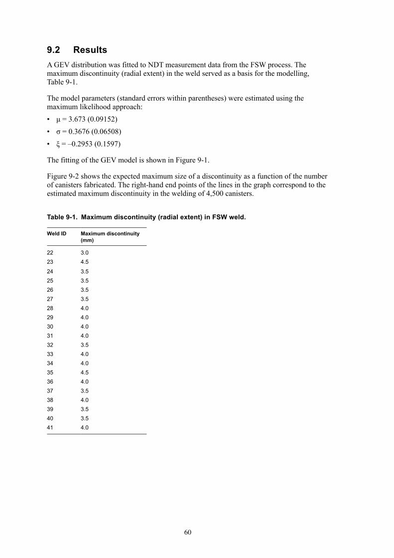
�0

9.2 ResultsA GEV distribution was fitted to NDT measurement data from the FSW process. The maximum discontinuity (radial extent) in the weld served as a basis for the modelling, Table 9-1.

The model parameters (standard errors within parentheses) were estimated using the maximum likelihood approach:• μ = 3.673 (0.09152) • σ = 0.3676 (0.06508)• ξ = –0.2953 (0.1597)

The fitting of the GEV model is shown in Figure 9-1.

Figure 9-2 shows the expected maximum size of a discontinuity as a function of the number of canisters fabricated. The right-hand end points of the lines in the graph correspond to the estimated maximum discontinuity in the welding of 4,500 canisters.

Table9-1. Maximumdiscontinuity(radialextent)inFSWweld.

WeldID Maximumdiscontinuity(mm)

22 3.023 4.5

24 3.525 3.526 3.527 3.528 4.029 4.030 4.031 4.032 3.533 4.034 4.035 4.536 4.037 3.538 4.039 3.540 3.541 4.0

�1

Figure 9-1. GEV model fitted to NDT measurement data (ultrasound) for the FSW process.

Figure 9-2. Estimated maximum discontinuity size, with confidence limits, in the production of different numbers of canisters.

Model (mm)

Mea

sure

d (m

m)

3.2 3.4 3.6 3.8 4.0 4.2 4.4

3.0

3.5

4.0

4.5

Number of canisters

Max

imum

dis

cont

inui

ty (m

m)

0.1 1.0 10.0 100.0 1000.0 10000.0

3.0

3.5

4.0

4.5

5.0

5.5

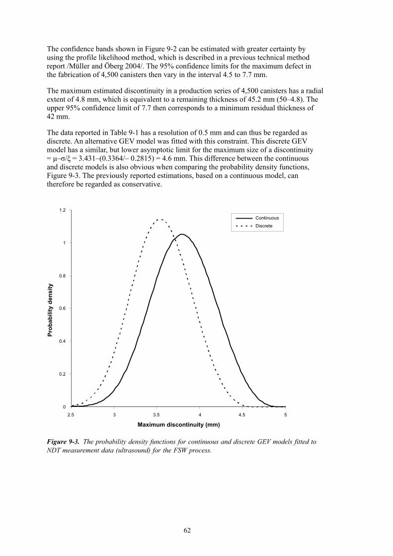
�2

The confidence bands shown in Figure 9-2 can be estimated with greater certainty by using the profile likelihood method, which is described in a previous technical method report /Müller and Öberg 2004/. The 95% confidence limits for the maximum defect in the fabrication of 4,500 canisters then vary in the interval 4.5 to 7.7 mm.

The maximum estimated discontinuity in a production series of 4,500 canisters has a radial extent of 4.8 mm, which is equivalent to a remaining thickness of 45.2 mm (50–4.8). The upper 95% confidence limit of 7.7 then corresponds to a minimum residual thickness of 42 mm.

The data reported in Table 9-1 has a resolution of 0.5 mm and can thus be regarded as discrete. An alternative GEV model was fitted with this constraint. This discrete GEV model has a similar, but lower asymptotic limit for the maximum size of a discontinuity = μ–σ/ξ = 3.431–(0.3364/– 0.2815) = 4.6 mm. This difference between the continuous and discrete models is also obvious when comparing the probability density functions, Figure 9-3. The previously reported estimations, based on a continuous model, can therefore be regarded as conservative.

Figure 9-3. The probability density functions for continuous and discrete GEV models fitted to NDT measurement data (ultrasound) for the FSW process.

0

0.2

0.4

0.6

0.8

1

1.2

2.5 3 3.5 4 4.5 5

Maximum discontinuity (mm)

Prob

abili

ty d

ensi

ty

Continuous

Discrete

��

9.3 PredictionerrorandmeasurementuncertaintyThe parameters in the extreme value model were estimated from the maximum discontinu-ity detected by ultrasound in the lid welds on 20 canisters. The confidence limits express the uncertainty in the parameter estimates. The best estimate of the maximum defect after fabrication of 4,500 canisters is thus 4.8 mm, but the uncertainty in the parameter estimate means that it is only possible to stipulate with certainty the that the maximum size will not exceed 7.7 mm (95% confidence limit).

Measurement uncertainties contribute to the uncertainty of the parameter estimate. A series of comparisons between ultrasonic testing and destructive testing indicate that the standard deviation is approximately 1 mm. This random part of the measurement error contributes to the parameter uncertainty and is included in its description. Beyond this there is also a systematic deviation that needs to be added to the model estimates. It is possible to use the mean of the residual values as a measure of the systematic deviation, but at least for joint line hooking the measurement error is systematically dependent on the discontinuity size. A conservative estimation is therefore to add the maximum measured discontinuity that entails an underestimation to the previously stipulated confidence limit for maximum size, i.e. 7.7 + 2.1 = 9.8 mm. If both parameter uncertainty and systematic measurement error are taken into account, it is reasonable to assume a maximum discontinuity size of 10 mm in the future production of sealing welds under the same conditions as during the trials described here.

The expected maximum discontinuity is dependent on the number of canisters fabricated, but when the upper confidence limit is estimated with the profile likelihood method, the differences are small. The maximum discontinuity, including measurement error, can be estimated to be 7.8, 8.9 and 10.3 mm for a production series of 100, 1,000 and 10,000 canisters, respectively. Consequently, the minimum copper coverage within the entire planned fabrication interval should be estimated at 4 cm for a 5 cm thick canister.

9.4 ProcesswindowinfutureproductionAs Table 9-1 shows, the maximum discontinuity varied between 3.0 and 4.5 mm during the demonstration series. Tests to optimize the length of the tool probe were carried out after the demonstration series and showed that a probe length reduction of 2 mm resulted in a variation of the maximum discontinuity between 2.0 and 3.0 mm during the 8 most recent lid welds. Trials with a reverse direction of rotation with a mirror tool probe have shown that the JLH can be reduced below 1 mm.

The fully automated weld cycle that is under development (see Chapter 14) is expected to increase the repeatability and reliability of the welding process due to the fact that software can control the adaptive welding process more quickly and reliably than a welding operator (human factor). A fully automated weld cycle also facilitates optimization of the welding variables for high stability and repeatability within as wide a process window as possible. Automatic control, together with an optimal process setting, is therefore expected to increase the size of the process window and result in a more reliable welding process. Furthermore, automatic control will in all likelihood lead to smaller natural variation within the process window.

��

10 Acceptancecriteriafordiscontinuities

As is evident from Chapter 4, the welding process is robust and generates welds of very good quality over a wide process window. The reproducibility of the process is also very good, as shown by the demonstration series. The verification experiments (Chapter 4) show that it is possible to control the welding process by controlling the welding variables. By logging the variables it is possible to ensure afterwards that the process has been kept within the permissible process window.

10.1 StrategyThe objective in formulating the acceptance criteria for the Sealing Subsystem is to guarantee the predicted future production quality. This means that the criteria must include limits for the welding variables, but also guarantee a robustness against possible unidenti-fied disturbances, which requires an independent NDT inspection step.

The steps in the inspection of the weld are shown in Figure 10-1 below.

10.2 AcceptancecriteriaThe weld’s inspection criteria consist of two parts that include both the welding process and the weld metal.

10.2.1 Thefirstacceptancecriterion

Theweldingvariablesinsealingshallliewithintheprocesswindow.

The smallest copper coverage on any canister in future production can then be estimated at 4 cm. The process window is defined in Table 4-8. Changes and improvements in the process and the welding system may require further studies of the process window. In conjunction with qualification of the welding process, a Welding Procedure Specification (WPS) is normally compiled. A WPS includes requirements on the tolerances of variables.

Figure 10-1. Schematic diagram of weld inspection against various criteria.

Welding

Process control/monitoring

Evaluation

Criterion 1

NDT

Final inspection

Evaluation

Criterion 2

��

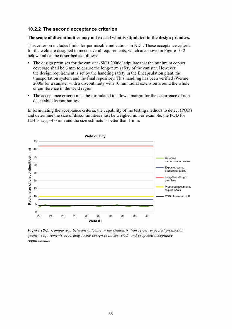
10.2.2 Thesecondacceptancecriterion

Thescopeofdiscontinuitiesmaynotexceedwhatisstipulatedinthedesignpremises.

This criterion includes limits for permissible indications in NDT. These acceptance criteria for the weld are designed to meet several requirements, which are shown in Figure 10-2 below and can be described as follows:• The design premises for the canister /SKB 2006d/ stipulate that the minimum copper

coverage shall be 6 mm to ensure the long-term safety of the canister. However, the design requirement is set by the handling safety in the Encapsulation plant, the transportation system and the final repository. This handling has been verified /Werme 2006/ for a canister with a discontinuity with 10 mm radial extension around the whole circumference in the weld region.

• The acceptance criteria must be formulated to allow a margin for the occurrence of non-detectable discontinuities.

In formulating the acceptance criteria, the capability of the testing methods to detect (POD) and determine the size of discontinuities must be weighed in. For example, the POD for JLH is a90/95=4.0 mm and the size estimate is better than 1 mm.

Figure 10-2. Comparison between outcome in the demonstration series, expected production quality, requirements according to the design premises, POD and proposed acceptance requirements.

Weld quality

0

5

10

15

20

25

30

35

40

45

22 24 26 28 30 32 34 36 38 40

Weld ID

Rad

ial s

ize

of d

isco

ntin

uitie

s(m

m)

Outcomedemonstration series

Expected worstproduction quality

Long-term designpremises

Proposed acceptancerequirements

POD ultrasound JLH

��

Definitions

Definition of coordinate system in assessment of size and position (see Table 10-1 and Figure 10-3) and explanation of different terms (see Table 10-2).

Table10-1. Explanationofcoordinatesystemincanister.

Symbol Explanation Unit

Dx Distance in radial direction between discontinuity and outer shell surface of canister. mmDy Distance in tangential direction between discontinuity and starting point of weld. °

Dz Distance in axial direction between discontinuity and top side of lid. mm∆x Distance in radial direction between discontinuities. mm∆y Distance in tangential direction between discontinuities. mm∆z Distance in axial direction between discontinuities. mmSX Size in radial direction. mmSy Size in tangential direction. mmSz Size in axial direction. mm

Figure 10-3. Definition of coordinate system in weld.

��

Table10-2. Explanationoftermsforacceptancecriteria.

Term Explanation

Discontinuity Imperfection in materialDetection level Signal level used for nondestructive testing for reporting of discontinuities. This level

is optimized to minimize the risk of false calls and ensure as good POD as possible.Indication Signal from nondestructive testing that exceeds defined detection levelInteracting discontinuity

Distance tangentially (∆y) less than 15 mm is classified as interacting discontinuities.

Defect Discontinuity that exceeds acceptance criteria

Proposed acceptance requirements

Table 10-3 below presents the proposed acceptance requirements for NDT. These requirements are set in the light of what can be regarded as reasonable levels to enable qualification of NDT. They are also set to provide margin to the expected weld quality in future production.

Table10-3. Proposedacceptancerequirements.

Term Requirement

Remaining wall thickness At least 40 mm copper coverage in radial direction.

Size determination in radial direction (SX) 3 mm.

Size determination in axial direction (Sz) 4 mm.Size determination in tangential direction (Sy) 4 mm.Radial position (Dx) 3 mm.Axial position (Dz) 4 mm.Tangential position (Dy) 4 mm.Maximum radial size (Sx), non-interacting discontinuities 10 mm.Maximum radial size (Sx), interacting discontinuities Total radial size 10 mm within cluster.Maximum tangential size (Sz) Whole circumference.

10.2.3 Requirementsfortestability

During ultrasonic testing of the weld, the ultrasonic signal is attenuated when it is transmitted through the top part of the lid. Investigations carried out during the course of the project have shown that the sound attenuation can vary both between different areas within a lid and between different lids. This should be taken into account when analyzing the investigation of the reliability of the NDT processes. Varying sound attenuation in both the lids used in the reliability study and those included in the demonstration series can affect the reliability of the NDT processes both positively and negatively. Investigations are under way to determine the extent of and find the reason for the variation of sound attenuation in the lids. When this phenomenon is understood, sound attenuation in the lids can easily be checked before welding so that its effect on the reliability of the NDT process can be estimated.

��

10.3 ApplicationoftheproposedcriteriaIf the criteria are not met, the sealed canister should be dealt with as a nonconformance. Examples of corrective measures for nonconformances are:• Rewelding: There is no reason why the canister cannot be rewelded by FSW. A weld that

fails to meet one of the criteria can, after study and correction of the welding system, be rewelded. If the acceptance criteria are met after rewelding, the weld can be approved.

• Rejection: Rejection is an option in the event of irreparable damage. For example, if the welding tool has broken and part of the probe is buried in the weld metal or a large geometric imperfection has arisen during welding.

• NDT approval: In the event of a small deviation from criterion 1, the weld can be approved provided that criterion 2 is met with good margin.

10.4 CommentsNDT in future production will primarily be used to verify the process and ensure that the premises regarding clear relationships between production quality and welding variables that have been demonstrated in this study apply. This means that production statistics based on NDT and welding variables in the process should be continuously analyzed and used to control the processes. Use of NDT will enable any currently unidentified error mechanism that arises in the welding process to be detected.

Due to the fact that the handling safety of the canister only has been verified for one case, a 10 mm discontinuity around the whole circumference is the acceptance criteria for the NDT limited. To be able to optimize these acceptance criteria, complementary calculations of the handling safety of the canister will be carried out. These calculations will most probably make it possible to increase the maximum radial size for isolated discontinuities and the allowed remaining wall thickness.

�1

11 MTOfactors

The work of designing and planning the future activities in the encapsulation plant is currently being pursued. MTO factors and their treatment will comprise an important part of this work. Based on the perspective of this report, however, there is good reason to describe in general terms how MTO is handled in the Sealing Subsystem.

Owing to the radioactive environment, the welding system must be remote-controlled and a high degree of automation is therefore required. Control and logging of process variables will also take place automatically. Evaluation of the welding process will, however, require human judgement in the evaluation of process variables. Like the welding process, the NDT system will be automated and remote-controlled. But here as well, human judgement is required in the evaluation of results.

To minimize the influence of MTO factors, the evaluation should be done by two inde-pendent judgement bodies, where the final judgement is made by an organisation that is independent of production.

Personnel who work with welding and NDT must have the requisite basic training and supplementary training for the task and be certified according to an appropriate system.

��

12 QualificationofprocesseswithinSealingSubsystem

The goal of a future qualification is to show that the processes in the Sealing Subsystem comply with:• Derived requirements regarding production pace and weld quality, structure and

composition /SKB 2006d/.• Reliability requirements regarding permissible variation in the process result.

Preliminary technical documentation for qualification is provided in this report for both the main processes, welding and nondestructive testing. A program for qualification is presented in /SKB 2006c/ and final versions of these documents are expected to be available in 2012.

12.1 WeldingInvestigations of the reliability of the Sealing Subsystem provide an important basis for the qualification work. In this context it can be noted that the process for welding of the bottom on the copper canister will be virtually identical to that used for sealing of the canister. The system for bottom welding will be identical in large parts, and the only difference is that the welding will be carried out on a horizontal canister. Control systems, welding tools and process windows will be identical in the two procedures. Considering the great robustness that characterizes the FSW process, it is SKB’s judgement that, after verifying tests, the same technical documentation can serve as a basis for qualification of this procedure as for sealing, but with a separate machine qualification.

Technical supporting documentation for qualification:• Studies showing the size of the process window.• Reliability of the logging of welding variables by the welding system.• Ability of the control system to keep the process inside the process window.• Calibration procedures for control and logging systems.

12.2 NondestructivetestingInvestigations of the reliability of the Sealing Subsystem provide an important basis for the qualification work. The process for testing of the bottom weld will, as in the case of the welding process, be virtually identical to the process for the sealing weld. The NDT system for the lid and bottom welds will be identical in large parts, the only difference being that NDT of the bottom weld will be carried out on a horizontal canister. As a consequence, it is SKB’s judgement that, after verifying tests, the same technical documentation can serve as a basis for qualification of the NDT process for both the sealing and bottom welds.

�4

Technical supporting documentation for qualification:• Description of possible discontinuities.• POD curves showing probability of detection.• Accuracy in size estimation.

12.3 AcceptancecriteriaThis report describes proposed acceptance criteria for the welding process and the welding system.

��

13 Conclusions

Based on the completed investigation, the most important conclusions are:• The welding process produces reproducible results which satisfy stipulated requirements

on minimum copper thickness with very good margin.• Control and logging of the welding variables can be used as a method to control the

process and approve a weld.• Nondestructive testing can be used as an inspection method for the process and with

adequate reliability as an independent inspection step.• The predicted outcome of the welding lies within relevant requirements with very

good margin.• The methodology for statistical experimental planning has been implemented with

good results and SKB plans to use this methodology for reliability studies of other subsystems in the production system.

��

14 Futurelineofaction

The development of the FSW process and the associated NDT process has gone very quickly. This report has shown that the processes that were developed up to the end of 2004 and that have been evaluated have very good potential to be used in a future production system within the Sealing Subsystem. The continued development work with the reliability of the process will be focused on further optimizing the process and verifying the results that have emerged in this investigation.

Further investigations concerning the connection between the welding variables and results from NDT will be conducted to further verify the conclusions in this report. Changes and improvements of processes and systems for welding will require further investigations of the process window. In conjunction with qualification of the welding process, a final version of the WPS (Welding Procedure Specification) will be prepared. The WPS includes requirements on tolerances, i.e. process windows for welding variables.

According to SKB’s timetable, final versions of all essential specifications and supporting documentation for the processes within the Sealing Subsystem must be available by 2011. This time span of five years provides time for technology development, optimizations and further evaluations.

14.1 ProcessFSWFurther development of the FSW process will be pursued according to the main lines presented in Table 14-1. More detailed plans are presented in /SKB 2006a/.

Table14-1. OverallplanofFSWactions.

Activity Contents

Automation of process.

The adaptive control of the process is currently manual. The software will be developed so that this can be done automatically so that the human factor can be minimized. This will also enable the process to be regulated more quickly and precisely.

Optimization of welding process.

When the automated software is fully developed, the process should be optimized towards high stability and repeatability within as wide a process window as possible.

The development work to increase the upper temperature limit of the process window and thereby also the safety factor will be pursued by testing new probe materials.

Evaluation of weld metal properties.

The influence of impurities on the properties of the weld metal will be further investigated. The purpose is to determine how they can affect the properties of the canister.

Acceptance criteria. As input to the final acceptance criteria will further investigations of the formation of discontinuities be studied. Furthermore, development of the process window will enable acceptance criteria to be established for the welding process.

��

14.2 ProcessNDTFurther development of the NDT process will be pursued according to the main lines presented in Table 14-2. More detailed plans are presented in /SKB 2006b/.

Table14-2. OverallplanofNDTactions.

Activity Contents

Optimization of NDT process.

The NDT process will be optimized by combining practical experiments with modelling of sound fields and their interaction with different types of discontinuities. The goal is to obtain an optimized NDT process.

Study of important variables.

Carry out a statistical study of which variables influence the NDT testing. The study is planned to be conducted according to principles similar to the study of the welding process.

Evaluation of material properties

Study what effects the properties of the lid material in terms of structure and discontinuities have on the NDT testing.

Acceptance criteria Formulate and adopt acceptance criteria based on supplementary knowledge from material examinations and the optimized NDT process.

14.3 OtherprocessesinproductionsystemforcanistersAnalogously with the investigations that have been conducted of process reliability for the Sealing Subsystem prior to SR-Can encompassing the welding process and subsequent NDT inspection, equivalent activities are planned for the Copper and Insert Subsystems prior to SR-Site. The timetable for these studies is shown in Figure 14-1 below.

Figure 14-1. Timetable for determination of reliability in the copper canister’s subsystems.

2006 2007 2008 2009

SR-Site

ReliabilitySealing Subsystem

Welding

NDT

SR-Can

ReliabilityInsert Subsystem

Fabrication

NDT

ReliabilityCopper Subsystem

Fabrication

NDT

��

15 References

AnttilaM,2005.Gamma and Neutron Dose Rates on the Outer Surface of Three Types of Final Disposal Canisters, Posiva Working Report 2005-14.

BoxGEP,DraperNR,1987. Empirical model-building and response surfaces. Wiley,

BoxGEP,HunterWG,HunterJS,1978.Statistics for experimenters: An introduction to design, data analysis, and model building. Wiley, New York, USA.

CederqvistL,2005. Friktionssvetsning av kopparkapslar rapport 1, SKB R-05-73. Svensk Kärnbränslehantering AB.

EfronB,TibshiraniR,1993.An introduction to the bootstrap. Monographs on statistics and applied probability. Chapman & Hall/CRC,xvi, New York, USA.

InternationalInstituteofWelding,1987.Guidance and recommendations on evaluation of ultrasonic signals in manual weld examination and on defect acceptance/rejection criteria.

MüllerC,etal.2006.Project NDT Reliability, final report,SKB R-06-08. Svensk Kärnbränslehantering AB.

MüllerC,ÖbergT,2004.Strategy for verification and demonstration of the sealing process for canisters for spent fuel,SKB R-04-56. Svensk Kärnbränslehantering AB.

RonnetegU,2005. Förstörande prov ur demonstrationsserie FSW, SKB rapport 1046524. Svensk Kärnbränslehantering AB.

RonnetegU,MobergB,2003.Inkapslingsteknik, Lägesrapport 2002, Oförstörande provning, SKB R-03-31. Svensk Kärnbränslehantering AB.

SamuelssonK-G,2005a.Sammanställning av resultat från bedömning av FSW-prover. Teknisk Rapport Bodycote CSM AB, TEK05-0402.

SamuelssonK-G,2005b.Dokumentation och uppmätning av skarvens utseende i FSW-prover, Rapport Bodycote CSM AB, PRO05-0487.

SaukkonenT,SavolainenK,HänninenH,2006. Microstructure of fiction stir welded copper joints, R&D Report, Posiva OY.

SKB,2003.Planning report for the safety assessment SR-Can, SKB TR-03-08. Svensk Kärnbränslehantering AB.

SKB,2004a.Programme for research, development and demonstration of methods for the management and disposal of nuclear waste, including social science research, Svensk Kärnbränslehantering AB.

SKB2006a.Kapsel för använt kärnbränsle – Svetsning vid tillverkning och förslutning, SKB R-06-04. Svensk Kärnbränslehantering AB.

SKB,2006b. Kapsel för använt kärnbränsle – Oförstörande provning av svetsar, SKB R-06-06. Svensk Kärnbränslehantering AB.

�0

SKB,2006c. Kapsel för använt kärnbränsle – Kvalificering av processer vid tillverkning och förslutning, SKB R-06-07. Svensk Kärnbränslehantering AB.

SKB,2006d. Kapsel för använt kärnbränsle – Konstruktionsförutsättningar, SKB R-06-02. Svensk Kärnbränslehantering AB.

SKI,2002. The Swedish Nuclear Power Inspectorate’s Review Statement and Evaluation ofthe Swedish Nuclear Fuel and Waste Management Co’s RD&D Programme 2001, SKI Report 02:33, Swedish Nuclear Power Inspectorate.

SwedishStandardsInstitute,2003.Welding and allied processes – Classification of geometric imperfections in metallic materials – Part 2: Welding with pressure SS-EN ISO 6520-2.

USDepartmentofdefense,1999.Nondestructive evaluation system. Reliability assessment, Handbook. MIL-HDBK-1823.

ÖbergT,2006a.SKB Canister Laboratory: Evaluation of process experiments with friction stir welding (FSW), TOMAS ÖBERG KONSULT AB MEMO-2004/5 rev. 2.

ÖbergT,2006b.Omräkning av responsytemodeller för FSW, TOMAS ÖBERG KONSULT AB MEMO-2005/10 rev. 1.

�1

16 Abbreviations

NDT Non-destructive Testing

POD Probability of Detection

ROC Receiver Operating Characteristic

UT Ultrasonic Testing

RT Radiographic Testing

FSW Friction stir welding

BAM Bundesanstalt für Materialforschung- und Prüfung

IC Intrinsic Capability

HF Human factors

AP Application parameters

μ-CT Micro-focus Computed Tomography

HECT High-energy Computed Tomography

MTO Man Technology Organization

��

Appendix1

NDTReliabilityProject leader: Ch. Müller(1),

C Bellon, S Bär, M Elagin, U Ewert, G-R Jaenisch, B Redmer, M Scharmach BAM – Federal Institute for Materials Research and Testing, Unter den Eichen 87; 12205 Berlin; Germany, Division VIII.3 Nondestructive Testing (NDT) and Characterisation; Radiology

R Boehm, U Tessaro, D Tscharntke BAM Division VIII.4 Nondestructive Testing (NDT); Acoustical and Electrical Methods; Ultrasonic Testing

J Goebbels BAM Division I.4 Nuclear Analysis

Abstract

This report “NDT reliability” describes methodology and results of the reliability investiga-tions performed by BAM for the non-destructive testing (NDT) methods developed at the SKB Canister Laboratory for the future canister manufacturing. On the one hand it creates a link from the assessment of the reliability and inspection performance to the full risk assess-ment process of the canister or deposit project. On the other hand it gives the confirmation of the basic quality of the NDT methods to verify they are suited to indicate the welding quality.

Additional reference X-ray examination using high sensitive technique and cross sectioning has been done to give a deeper confirmation of the welding quality down to a micro-struc-ture level. The probability of detection curves are in principle determined according to the MIL 1823 Reliability Guideline which was developed for the determination of integrity of gas turbine engines for the US military. Extensions for the more complex discontinuity situations in the copper stir friction and electron beam welds were necessary which are for both the welding and the NDT technique a challenge.

As the key parameter for the flaw detectability the a90/95 magnitudes are determined, i.e. the size a of the flaw for which the lower 95% confidence bound crosses the 90% POD level. This means it is guaranteed that flaws with a size of a90/95 will be detected with 90% probability where only 5% might fall outside this confidence limit in case the experiment is repeated.

ContentsA1 Introduction to the BAM “NDT Reliability Project” 84A2 Strategy 84A3 Test specimens – frictions stir weld (FSW) 89A4 NDT methods used at SKB 92A5 Reference methods for FSW Welds 93A6 Reliability assessment using POD 101A7 Summary of Results 118A8 Conclusions 119A9 References 120A10 Abbreviations 120

�4

A1 IntroductiontotheBAM“NDTReliabilityProject”

The “NDT Reliability Project” is a subpart of the risk assessment concerning the integrity of the sealing welds of the copper canisters due to defects occurring during the manufacturing process. It analyses the NDT techniques applied at the SKB canister laboratory concerning the question: “Which is the size of the defect which will be detected for sure or which is the size of the defect which might be overseen?”. The project delivers these values together with the underlying parameters (of the welding process, of the NDT set-up, of selection of defect features and of levels of confidence) to the further risk evaluation.

On the other hand it investigates the basic reliability of the NDT methods to make sure they are sensitive enough to accompany the development of the welding procedure as analysis method for any possible occurring defects. So the first task for the risk assessment is oriented to the higher end of possible defect sizes and the second part of basic reliability is oriented to mid part and lower end of possible defect sizes.

For the reliability analysis the basic guidelines of the American Military Standard MIL 1823 were applied with further development and adaption to the more complex testing task compared to the “one dimensional task” to detect cracks with eddy current in gas turbine engines. To be able to understand and optimize the state of the art performance of the NDT methods BAM is performing – especially for the X-ray equipment – detailed parameter measurements according to the present European standards. Because of the complexity and the uniqueness of the testing task and equipment both the parameter analysis of the experiments and the reliability investigations are assisted by modelling calculations.

The welding experiments and NDT-experiments are carried out at the canister laboratory in Oskarshamn. To learn about defect findings it is necessary to compare the NDT indications with the true defect situation in the welds. To indicate and characterize the true defects in the weld, specialized 3D tomographic methods of BAM were applied. The methods applied are for the weld as (almost) a whole by HECT (high energy computerized tomography) and on a smaller level towards micro-structure analysis using a micro-CT with highest possible X-ray energy (unique in Europe). The CT techniques provide the true indications for macroscopic volumetric defects instead of destructive cross sectioning and provide structure information plus confirmation of all smallest possible defect configurations instead of micro metallographic methods. Finally have destructive tests been performed to verify the CT-results.

A2 Strategy

A2.1 Subject

A subpart of the final risk assessment of the deep repository construction is to determine the risk of premature canister leak caused by discontinuities in the sealing weld. The discontinuities occurring during the production welding process create a diminishing of the wall thickness, which could affect the long-term integrity of the canister. The consequence for the applied NDT methods is to detect all discontinuities, which would reduce the wall thickness with a validated high reliability. This study has been based on a conservative assumption that the minimum copper wall thickness has to be 15 mm to guarantee the long-term integrity of the canister. Ongoing studies indicate however that the corrosion integrity requirement could be considerably lower.

��

The POD’s considered in this report reveal the basic, or intrinsic capability of the NDT methods and do not yet take into account the final industrial application factors and the human factor as shown in the “Reliability Formula” in Figure A2-4 which will be applied to the canister welds on a later stage of the project. This one reason we held on the very conservative integrity requirement throughout the project.

A2.2 Inspectiontechniques

The NDT systems to be analyzed were the X-ray system and the ultrasonic system at CL. The result of using the two inspection systems in combination was also analyzed.

The inspection task to study is the inspection of sealing welds produced using friction stir welding (FSW) technique.

The X-ray inspection system at CL consists of a 9 MeV Varian accelerator with a 16 bits AD and viewing system provided by BIR. The ultrasonic system is a phased array 10 bit system. The inspection of the weld is carried out using an 80 element array working at a centre frequency of 5 MHz. The NDT inspection systems at CL are described in Chapter 4.

From the physical point of view the two methods are complements to each other. In radiog-raphy the signal for defect detection is essentially the X-ray intensity difference in direction of the radiated length of the defect. In the ultrasonic is the echo intensity mainly propor-tional to the area perpendicular to the ultrasonic beam. Due to these facts the radiographic method is better suited for volumetric defects and the ultrasonic method for area-like defects. Though the modern phased array techniques applied in the project are capable to overcome these limitations by the additional degree of freedom in beam angle steering by electronic means the radiography will be kept as accompanying analysis method while the welding process development.

A2.3 StrategyfortheDeterminationofNDTReliability

The NDT Reliability is the degree to which the NDT system is capable to reach the intended aim in defect detection and characterization and considering false calls (Second European-American Workshop on NDT Reliability 1999). The intended aim of quality assurance and production control of lid welds of copper canisters are • To be able to, in quantitative terms, express the risk for failing to detect canisters

containing defects in the sealing weld that exceeds the acceptance criteria.

Figure A2-1. The weld with possible defect configurations.

Remaining wall-thickness must be at least 15 mm

Defect

Remaining wall-thickness must be at least 15 mm

DefectDefect

��

• Being able to define the measurement accuracy of the inspection in terms of defect size and location.

The work is aimed to result in a general methodology that can be applied for other inspec-tion tasks for the canister.

A2.3.1 StrategiesinMeasuringReliabilityofNDT

Three different ways to investigate the reliability of NDT signals will be described which are to a more or less greater extent applied during the project. The first way of investigation, the performance demonstration, is preferred e.g. in the US American nuclear power industry qualitatively and quantitatively in the aerospace industry. This is an integral consideration of the non-destructive test as a system where the whole NDT system is packed in a black box and only the input in terms of the real existing flaws in the component is considered. This is compared to the output in terms of the indications of the human inspector or of the automated system.

The second – the European tradition – relies on a standardized description of physical/technical parameters of the NDT system, which are preconditions for successful system performance. As example for such a standardized set of performance parameters the X-ray system of SKB is characterized completely against the existing European standards, which will be described in detail in the final report /9/.

The third approach – the modular conception – is a marriage of both: The signal chain is cut into main modules. Each module is assessed in a most appropriate individual way e.g. via modelling calculations. The single results are joint together according to the reliability theory of systems or in simpler cases by technical justification or physical reasoning.

The NDT system consists of the procedures, equipment and personnel that are used in performing NDT inspection. According to this definition we consider in the situation in Figure A2-2, where we have on the left hand side the “truth” of the component, which is in our case a weld with defects and on the right hand side the corresponding inspection pro-tocol with defect indications. This means that we have a 100% reliability when we would have a 1:1 correspondence between both sides. Since this is in almost all practical examples not the case we have to set up tools to measure and maintain reliability.

In Figure A2-3 we take a closer look to an NDT signal transfer chain: The signal starts in terms of an energy beam or wave from a source and interacts with matter in terms of a component and its possible defects creating an output signal which is driven by the physics of the method. This output signal is now further influenced by the physical and technical properties of the more or less complex receiver and converter. In our case this are the imag-ing item for X-rays and the digitization and processing unit.

Now we consider how to measure and ensure the reliability. We start with the European approach: This approach is by far the most widely used, and is in use in most, or perhaps all, industries. One or more reference objects (such as EN 462 image quality indicators for radiography, or ASTM E 127 reference blocks for ultrasonic inspection) are used, in combination with written procedures controlling details of the inspection method, to reach and demonstrate consistency. The intent is to achieve essentially the same inspection conditions, independent of where, when, or by whom an inspection is conducted.

This type of European approach is often used to provide process control information of a qualitative nature: loss of control at some earlier manufacturing stage is indicated by the unexpected occurrence of numerous or large indications, for example. Capability for

��

detection of “real” (naturally-occurring) defects is not given for all applications, but is sometimes inferred from the size of the simulated defects in the reference objects, or from the size of defects that have been detected in past inspections using the same conditions. This inferential process can often lead to false conclusions about the detectability of real defects.

The first step of a performance demonstration is also to define the essential technical parameters of the system. The ROC and POD methods are appropriate tools to provide a clear measure of integral performance of the system. It has though to be paid by high effort in test series with realistic test samples and should be completed by a series of affordable “computer experiments” using theoretical modelling techniques. With POD the user can learn about the detection capability whereas the ROC gives more information about the system’s capability to distinguish between signal and noise. The modular approaches open the door to a promising technique – more efficient and with the capability also to optimize the system.

Figure A2-2. The Aim of NDT – Describe the real status.

Figure A2-3. The Signal Transfer Chain of a Radiographic System.

��

A2.3.2 SelectionofReliabilityDataEvaluationMethodstobeappliedforSKB–General

Since the main goal is a high precision assessment of the flaw size, which might be overseen by NDT, the quantitative POD (Probability of Detection) method according to MIL-STD 1823 /5/ was selected for this assessment. The (1 – POD) curve will provide the probability of missing a defect as function of defect size. This can be used as input for probabilistic risk assessment of failing with the assumption of a certain flaw growth behaviour under a certain load.

The conventional procedure provides a mean POD-curve as function of defect size with a corresponding 95% confidence limit curve due to the scatter in the experimental values. The defect size “a” which is counted as practically sure detectable, is when the 95% confidence limit curve reaches the 90% POD level. For all applied methods it has to be shown that this size “a” or better its projection/component in radial dimension is smaller than the allowed defect size (35 mm). The POD level also gives a quality feature about the NDT method showing which defect sizes are detected for sure.

A2.3.3 SignalPOD,HitMissandROCandplanofexperiments

Both SKB-NDT-Methods are 100% digitized and fully mechanized methods so that a full signal analysis is possible according to the “â versus a” method. The method analyzes the full potential power of the NDT method to detect a signal “â” from a noisy background caused originally by a physical defect dimension of size “a” in the object under test. The shape of the final POD-curve depends on the selection of the threshold from which on a signal is counted as a real signal from a defect in contrast to a noise signal.

Considering the reliability formula in Figure A2-4 this covers mainly the assessment of the intrinsic capability and controlled application factors. As long as human beings carry out the signal detection “a” so called “hit miss” POD has to be determined where the Human Factor is also assessed via a statistically reliable experiment using a number of different human interpreters. These results will then further be analyzed via the ROC method as described above to allow to select the optimum operation point also with respect to the economy of false calls.

Figure A2-4. Identifying the main influencing factors by the reliability formula.

��

The current report is focused on the intrinsic capability of the ultrasonic technique and the radiographic technique to detect all possible and relevant defects in the FSW-welds which was selected as the main welding technique in April 2005. The FSW welding technique and the formation of defects is a “new land” for NDT techniques as well as their reliability assessment. So while demonstrating that the techniques are basically capable of meeting the safety requirements, they are still under further development including the multidimen-sional/multi-parameter POD approach.

For the safety relevant reliability assessment, of the intrinsic capability and part of appli-cation factors of NDT- reliability, the signal-POD (or â versus a) method according to Mil 1823 is already well suited to determine the remaining probability of the applied NDT method to oversee a defect of a certain size. The originally 1- dimensional conception can be used in defining “effective” 1D parameters. A comprehensive treatment of the problem, especially in separating all the physically influencing factors from the factor of interest, the radial dimension of the defects, the full 2D approach needs to be applied in further project stages. To cover possible gaps in the empirical evaluation schemes high-qualified modelling techniques are applied to complete the physical reasoning of the results and to provide a broader parameter range than possible from the real experiments.

The common approach is to determine the real defect sizes via destructive tests. In the original approaches, in the gas turbine industry, the defects were even surface cracks to be easily measurable via optical surface methods. In our approach a high value was assigned to the possibility to have still access to the complete defects in the welds even in sections. When they are once destroyed no more reconstruction of the full 3D situation is possible since during destructive tests parts of information get lost. For this reason a full 3D high energy CT /6/ is used as reference methods to characterize all volumetric defects down to 1mm diameter. The final validation was done for all defects via destructive tests and metallographic inspection.

A3 Testspecimens–frictionsstirweld(FSW)

This chapter gives a brief description of the friction stir objects that have been used in this study regarding welding process, geometry and possible discontinuities. A more detailed description is made in the main report.

A3.1 Weldingprocess

FSW was invented at The Welding Institute (TWI) in 1991 and is a solid-state thermo-mechanical joining process, which is a combination of extruding and forging. A cylindrical, shouldered tool with a profiled probe (pin) is rotated and slowly plunged into the material (Figure A3-1). For thick sections, a pilot hole has to be drilled to make the plunge sequence possible without probe fracture. Frictional heat is generated between the wear-resistant tool shoulder and the material, causing the material to soften without reaching the melting point, and allowing the tool to traverse the joint line.

One reason for the rapid success of FSW is the ease of process control due to the relatively few input parameters. The tool is rotated at a specified rotation rate and the tool is traversed along the joint line at a specified traverse rate. The tool is usually also tilted relative to the work piece so that the leading edge is above the surface. The tool shoulder to work piece penetration is then controlled by applying a specified downward force or by specifying the position of the shoulder relative to the work piece. In addition to the input values, the tool temperature and the spindle motor torque are measured which provides an indication of the state of the process and the amount of frictional heat generated.

�0

A3.2 Geometry

As the welding process starts and stops above the joint line, the lid has extra material, which is machined after welding to get a smooth surface for the NDT. The geometry of the lid weld is shown in Figure A3-2.

Figure A3-1. Welding process.

Figure A3-2. Joint design friction stir welding.

Machining lines

Weld area

Joint line

50 mm

50 mm

�1

A3.3 Discontinuitiesfoundintheproject

During the welding trials at the Canister Laboratory have two types of defects been found when relevant process parameter settings have been used. These two types can be called wormholes and joint line hooking (JLH). The wormholes can be located in the outer part of the weld and are more or less volumetric (see Figure A3-3) while the JLH is located in the weld root and are non-volumetric, see Figure A3-4 below.

Figure A3-3. Location of discontinuities in FSW.

Figure A3-4. Wormhole (a) and Joint line hooking (b).

Joint line hooking

Wormholes

�2

A4 NDTmethodsusedatSKB

The NDT techniques that are used for inspection of the welds are high-energy digital radiography and phased array ultrasonics. This chapter describes the main principles, while a more detailed description is made in the main report.

A4.1 Digitalradiography

The method for digital radiography is based on a 9 MeV linear accelerator: The accelera-tor generates X-rays, which are transmitted through the weld with an incident angle of 35° against the horizontal axis while the canister rotates. A vertical linear detector placed perpendicular to the beam detects the penetrated radiation (see Figure A4-1).

A4.2 Phasedarrayultrasound

The phased array ultrasound inspection is made from the top of the lid. The method use a linear array, which electronically scan in the radial direction (beam steered with incident angles within –20° to 20°) the while the canister rotates, see Figure A4-2.

Figure A4-1. Principles of radiography of FSW.

Detector

Weld

X-rays

��

A5 ReferencemethodsforFSWWelds

A5.1 Destructivetesting

To verify the real size of the indicated discontinuities have destructive tests been performed at SKB. As the characteristics of the different types of discontinuities varying, have different techniques for determine the sizes been used.

For the joint line hooking type have following methodology been used:• From the weld surface have cores with 40 mm diameter been drilled at positions where

NDT have indicated presence of discontinuities. • The cores have been split into two halves, see Figure A5-1. • One of the halves have then been polished and etched.• Finally have the discontinuities been characterized with a microscope, see Figure A5-2.

To determine the sizes of the wormholes have following methodology been used:• From the weld segments (FSW5) have areas where discontinuities indicated by NDT

been marked. In this areas have cubes of the size of 50 mm been machined, see Figure A5-3.

• The cubes have been X-rayed in three directions at the Canister Laboratory to locate the discontinuities.

Figure A4-2. Phased array ultrasound inspection.

�4

Figure A5-1. Core for destructive evaluation of joint line hooking.

Figure A5-2. Macrograph of the joint line hooking in weld FSW27.

• Four of these cubes have finally been machined step by step with increment of 0.1 mm and for each slice have the discontinuities been documented by digital camera.

• Finally the discontinuities on the digital photos (Figure A5-4) have been grouped into clusters and the sizes have been determined.

��

A5.2 ComputedtomographyHECT

The multi-purpose computed tomography system developed at BAM /8/ works with different combinations of radiation sources and detector systems. For high attenuation materials like Copper an electron linear accelerator (LINAC) is used as X-ray source (Energy: 10.5 MeV; Dose 15 Gy) together with an amorphous Silicon flat panel detector with 256×256 pixel. The pixel size is 0.8×0.8 mm2. Figure A5-5 shows an overview of the multi-purpose tomograph with the LINAC at right and the flat panel detector at left.

Figure A5-6 shows the flat panel detector en detail together with a Cu sample on the scanner table.

Figure A5-3. Copper cubes for destructive evaluation of wormholes.

Figure A5-4. Photograph at 6.2 mm depth of wormholes in weld FSW5.

��

Figure A5-5. Multi-purpose-Tomograph of BAM with the LINAC X-ray source at right and the flat panel detector at left.

Figure A5-6. Display detail of flat panel detector and Cu sample on the scanner table. The electronic part of the detector was shielded against X-ray radiation with 20 cm of lead.

��

Due to the magnification, that means the ratio of distance source-detector to distance source-centre-of rotation of the scanner table, the pixel size in the object plane is 0.65×0.65 mm2 That means that a cylindrical sample volume with a height of about 140 mm can be measured in one cycle. Therefore the Cu samples with a height up to about 30 cm are measured in three different heights and the overlapping volume image data sets are merged to a geometrical correct overall data set.

Each of the three partial volumes of the sample was measured with 720 projections over 360°, the integration time per projection was 0.8 sec. Due to the angular over-sampling the data could be reconstructed in an image matrix of 511×511×255 voxel with an voxel size of (0.325 mm)3.

The result of the measurement is the material dependent linear attenuation coefficient µ, averaged over one voxel, the unit is cm–1. For an image representation these values are normalised to 8 Bit:• Grey level 0 ↔ µ = 0.0 cm–1

• Grey level 250 ↔ µ = 1.7 cm–1

assuming the attenuation value for air is µ = 0.0 cm–1, which is valid for the used high X-ray energies.

There are mainly two sources of artefacts:• the energy spectrum of the X-ray source, resulting in beam hardening artefacts,• inherent properties of flat panel detectors.

To eliminate beam-hardening artefacts the energy spectrum of the LINAC is filtered by 90 mm Fe. The fact that flat-panel detectors are not collimated leads to some artefacts, especially that edges are smoothed. Therefore a pre-processing step of the raw data was performed, a high-pass convolution filter.

The back-projection of the raw or pre-processed data is done by the well-known Feldkamp algorithm. Figure A5-7 shows a vertical slice from the image data set of the reconstructed raw data after pre-processing.

For the further processing the voxel-based data format are converted to the ‘stl’-data format using a threshold operation. Due to the detector limitations smaller flaws are handled sepa-rately using Region-of-Interest operations. Simplified this means that for small flaws object depending thresholds are used. The different steps of image processing tools hereby are:• Segmentation of the envelope of the sample, setting of a threshold and conversion to

the stl-format.• Segmentation of single flaws, setting of a threshold and conversion to stl-format.• Merging of the different stl-data sets of the envelope and the isolated flaws.

��

A5.3 EvaluationofFSWtestsamplesbyradiography

SKB delivered 20 extra test samples to be investigated by micro CT in addition to the specimen investigated for the POD analysis. Since the micro-CT equipment ws out of order for a longer time period BAM performed additionally standard Radiographs from two directions with a Seiffert Tube (320 kV) used at 270 KV for optimum contrast (set up see Figure A5-8).

X-Rayparameters Legend

Volatage 270 kV Seiffert 320 kV

Current 5 mA

focus size 1.5 mm

film-focus-distance 1,000 mm

film Agfa D2

screens Pb 0.02×0.02 mm

exposure time 6 min.

optical density 2.6

(inside object)

JLH? – suspicion of Joint Line Hooking

Figure A5-7. Vertical slice from the 3D image data set after pre-processing of the raw data with an high-pass convolution filter.

��

The only indications are “tails” from the JLH type of flaws, which are described, in former chapters.

Figure A5-9 shows the radiographic images of example indications of the JLH.

TableA5-1. EvaluationresultsofradiographsoftheFSW-testsamples.

SKB:FSW-samples(Cu)forMicro-CT(sizesinmm)

Film/ImageIndentification

Evaluationresults

0° 90°

FSW28/202 20×20×49 9 +XFSW31/280 20×20×49 10 +XFSW33/39 20×20×49 11 +XFSW37/33 20×20×49 12 +XFSW22/201 20×20×80 13 +X linear indication (gap)

suspicion of JLH? FSW23/143 20×20×80 14 +XFSW24/264 20×20×80 15 +XFSW25/79 20×20×50 16 +XFSW26/225 20×20×80 17 +X linear indication (gap)FSW27/260 20×20×80 18 +X linear indication (gap)FSW29/205 20×20×80 19 +XFSW30/39 20×20×80 20 +X linear indication (gap)FSW32/199 20×20×80 21 +X linear indication (gap)FSW34/233 20×20×80 22 +X linear indication (gap)FSW35/100 20×20×80 23 +XFSW36/109 20×20×80 24 +X linear indication (gap)FSW38/315 20×20×80 25 +X linear indication (gap)

suspicion of JLH? FSW39/39 20×20×80 26 +X linear indication (gap)FSW40/347 20×20×80 27 +X linear indication (gap)FSW41/154 20×20×80 28 +X

Figure A5-8. Radiographic set up for the Cu-blocks.

100

Figure A5-9. Examples of indications in radiographs.

101

A6 ReliabilityassessmentusingPOD

A6.1 MethodologyforPOD

The basic principle of the signal response analysis or “â versus a” evaluation is shown in Figure A6-1. A defect of size a (crack depth in Figure A6-1) is causing a signal of height â. The statistical distribution of the signals in dependence of the defect size yields a certain POD-curve, which is described in more exact terms in the following section.

A6.1.1 âvsaanalysis

A6.1.1.1 General description /1/

Consider a quantitative NDT system. As a result of the investigation of a discontinuity having size a, it generates a signal â. If the signal exceeds a certain decision threshold âdec, the system registers a discontinuity detection. As the NDT system is influenced by uncontrolled factors, discontinuities of the same size can cause signals of different strength. For this reason the strength of the signal â to the discontinuity of size a is considered as a random value and associated with a probability density ga(â). The relation between a and â can be expressed as follows:

â = μ(a) + δ (1)

Here μ(a) equals the mean value of ga(â) and δ is the random error whose distribution determines the probability density ga(â).

Figure A6-1. Quantification of the risk: “â versus a”.


aâ

a â POD





response

typical POD

POD

a

100 %

log a

log â



aâ

a â POD





response

typical POD

POD

a

100 %

log a

log â



aâ

aâ

a â POD





typical POD

POD

a

100 %

log a

log â POD

a

100 %

log a

log â

response

102

In practice, it is often assumed that δ is distributed normally with zero mean and constant (independent of a) variance. ga(â) is then the normal density function with mean μ(a)=0 and variance equal to that of δ.

The probability of detection (POD) as function of the size of the discontinuity is given by:

(2)

Figure A6-2 illustrates this formula. The probability of detection is represented as hatched part of the area under the bell curve.

A.6.1.1.2 Calculation of the POD

Source data are a and â – arrays of length n that contain sizes of the defects and response magnitudes, respectively, and the decision threshold âdec. Note that the theory for deal-ing with censored data has been developed /1/ but is not used here, because the data sets available to us do no contain censored data. The censored data are the signals that cannot be registered by the system because they are either under the recording threshold or above the saturation threshold.

Figure A6-2. Probability of detection.

10�

A6.1.1.3 Calculation of the POD function parameters

The following formula is commonly used to model the relation between a and â:

ln â = β0 + β1 ln a + δ (3)

Here δ is normally distributed with zero mean and constant variance .

Under the assumptions of the model, the POD function has the following form:

(4)

where Φ is the standard normal distribution function, and (5)

(6)

The parameters β0, β1 and σδ describe the linear dependency of â on a and have the following meaning:

β0 Interceptβ1 Slopeσδ Standard deviation of the residuals

Their values are estimated from the arrays a and â using the method of maximum likelihood.

A6.1.1.4 The 95% lower confidence POD

The 95% lower confidence bound is given by the following formula:

POD95 (a) = Φ (z –h) (7)

where the variable h reflects the sample size and the scatter of the source data. The calculation of h is thoroughly described in /1/.

This general formalism has now to be applied to the defect detection problem within the scope of welding optimization and risk assessment.

A6.1.2 POD–theoriginaltask(fullprogram)

The original task (together with the welding optimization) is to make sure that only one of 1,000 canisters might contain a critical defect situation where in total more or equal 35 mm of the Cu-wall is missing.

From the naturally real existing POD as a function of all possible influencing parameters we have to extract the POD as function of the flaw radial dimension by a dedicated “Plan of Experiments” and reasonable mean value operations (see formula (8) below). The full program is only feasible with a number of additional experiments. But in order to learn where we are with our current NDT technique and where to optimize, we need a POD assessment of the state of the art using a “Preliminary POD Assessment”.

POD = f (a1,..., an) → POD = g (aradial) (8)

104

A6.1.3 AdaptedPODassessment

Volumetric discontinuities and area-like (non-volumetric) discontinuities will be treated separately • volumetric discontinuities RT and UT• area like discontinuities UT

The physically reasonable “â versus a” POD including physically reasonable 2D extensions will be applied to the parameter configurations shown on Figure A6-3.

A6.1.3.1 Explanation for the Assignment of a and â

Radiography RT

The physical reason for a signal (contrast) of a flaw in a radiographic image is the differ-ence in penetrated length of material (Cu) along the X-ray beam caused by the dimension of the flaw in beam direction which we call “penetrated length”. The contrast is the difference of the intensity behind the flaw with respect to the intensity Ib (b for background) behind the bulk material without the flaw. We apply the definition of the contrast derived from the absorption law according to ASTM E 1000, p 438 /3/

I = I 0e–μ ∆w (9)

From this the exact expression for a wall thickness difference – in our case equivalent to penetrated flaw length – would be

ln I1 – ln I2 = μ∆w and ∆w = w2 – w1 (10)

where I1 is the intensity behind the flaw and I2 the intensity behind the bulk material in the surrounding.

For small ∆w (with respect to the total penetrated wall length) we get

∆I = I × μ × ∆w (11)

where we assume the I to be an almost constant “working point” Ib of the radiographic system.

The penetrated length is the intersection of the flaw with the beam with its 35° incident angle according to the set up of the RT system.

Figure A6-3. Assignement of a and â for RT and UT.

10�

Ultrasound UT

According to the MIL 1823 handbook for reliability assessment /2/ Appendix C the UT echo height behind the flaw is recommended as the signal response “â” and as the causing flaw dimension “a” the reflecting area of the flaw. The ASNT NDE handbook recommends /4/:

“The height of an echo depends on the size (reflecting area) of the discontinuity, its depth, shape, orientation and the nature of the test object surfaces (roughness, contour and acoustic impedance). When the discontinuity is smaller than the diameter of the sound beam, the size maybe deduced from the height of the echo, provided the following essential conditions are fulfilled: 1. the plane of the discontinuity must be parallel with the sound entry surface, 2. surface roughness less than 200 µm, 3. the reflectivity is 100 percent and the discontinuity distance from the sound entry surface

is in the far field and there is no edge interference.”

For the application of the POD concept using “â versus a” the precondition is, that the echo height will in principle grow with defect size. There will be of course a scatter due to the uncomplete fulfilment of the points (1), (2) and (3) especially point (2) for the discontinui-ties in FSW. These types of scatter are taken into account in the POD calculation. Important is that the scatter due to other influences is not completely overwriting the principal grow-ing with size.

As will be seen in the following detection diagrams all flaws thicker than or equal to 1mm (in Z direction of the experimental system) are well indicated by the RT system. Therefore we call these flaws “volumetric flaws”. The flaws thinner than 1 mm and with a minimum area of about 4 mm2 are well seen in the UT scans and we will call them “area like” or “non-volumetric” flaws. The flaws with thickness smaller 1 mm and area smaller than 4 mm2 we are gong to call indifferent material discontinuities.

As the basic parameter for the flaw detectability /1/, /2/ we determine the a90/95 magnitudes, i.e. the size a of the flaw for which the lower 95% confidence bound crosses the 90% POD level, This means it is guaranteed that flaws with a size of a90/95 will be detected with 90% probability where only 5% might fall outside this confidence limit in case the experiment is repeated. We work with the assumption – given by the manufacturing experts – that only one of 100 canisters might have a critical flaw. Then the above argumentation yields: Only each of 1,000 canisters might have a leakage.

A6.1.4 Integrityrequirement

The flaw radial size has to be limited so that a remaining wall thickness of 15 mm is guaranteed against ground water corrosion. The maximum allowed flaw size in the radial direction is 35 mm. Together with the above POD an additional flaw geometry statistics has to be provided for the discontinuities that shows that no flaws of ar ≥ 35 mm will be present. No flaw of radial size ar ≥ 35 mm can be among the flaw assembly below a90/95, that means no a ≤ a90/95 should have at the same time an ar ≥ 35 mm. This would yield a reasonable justification of the system to meet the above integrity requirement, as long as the existing flaw configurations are representative for the welds. Look for the “correlation” in scatter diagrams titled “Critica Region …” below:• penetrated flaw length by X-ray ↔ radial dimension,• area perpendicular to UT beam ↔ radial dimension.

10�

A6.2 PODevaluationfromexperimentaldata

Steered by the plan of experiments for the welding procedure optimization and verification, the POD (Probability of Detection) for the defects is determined using a systematic statisti-cal methodology. The POD method, where the detection probability is determined as a function of defect size, was originally developed for the US military aerospace sector /2/ for 1-dimensional signals. For the more complex 3-dimensional defect situation in the canister welds and 2-dimensional data fields the method needs to be developed further. From the POD-curve and its lower confidence bound the defect size is derived that will be detected with sufficient reliability and compared to the demand for integrity. This procedure includes series of experiments with the SKB X-ray and ultrasonic methods foreseen for the produc-tion.

These results have to be compared to true defect configurations in the welds. To determine these “true defect configurations” the welds have to be tested destructively or tested with a more comprehensive non-destructive reference method. To get a complete 3D view to the flaws, the BAM selected a high-energy computed tomography (HECT, or CT) method as reference for volumetric flaws. The CT-results were at the end compared to destructive measurements. For the area like “JLH-defects” only destructive testing could be applied as reference. Figure A6-4a shows an example of a cross section of a wormhole and Figure A6-4b shows several spatial vies on this flaw from the CT data.

A6.2.1 Results

In the following diagrams we illustrate the results for the “preliminary POD” for UT and RT for the wormhole type of flaw in stir friction welds. In principle the wormholes are to some extent in between volumetric and area-like flaws. Since so far no flaws were observed in and below the order of magnitude of 1mm the argumentation for the overall reliability will be completed by the model calculations in the next chapters discussing the small flaws for RT detection.

Figure A6-4. Cross section FSW5-136 (a) and CT wormholes (b).

10�

The joint line hooking flaws are clearly area like. They are very flat (Z-direction) and of longer extent in the circumferential direction. So the illuminated flaw size in circumferential direction is determined by the sound beam diameter of about 5mm yielding a constant factor for the expression of the area perpendicular to the sound beam. So for this flaw type the POD diagrams were set up as a function of the radial dimension as asked for in the integrity requirement.

A6.2.1.1 RT wormhole

Below the “Adapted POD Results” for the wormholes for RT- and UT-inspection are presented with the following pattern: First the “â versus a” scatter diagrams is presented where the â’s in terms of maximum radiographic contrast and the maximum echo height, respectively are plotted in dependence on the “a” in terms of penetrated length and area perpendicular to the sound beam. For these signal sizes the actual thresholds are applied yielding the mean POD-curves and the 95% confidence bound and the a90/95 as key parameter. As discussed above the additional scatter diagram showing the statistics of the “a” dimension in dependence on the radial dimension reveals for all cases that the “critical” region with critical radial dimensions belonging to “a”-values below a90/95 are far away from the actually occurring configurations.

To find always the adequate reference and to be able to compare UT and RT signals the working term “flaw groups” were introduced for the wormhole type flaws.

One problem that arises while comparing the results of the inspection by different NDT techniques is the comparability. Often the same group of flaws is represented as varying number of indications on the images obtained by radiography and ultrasound. Consider the Figure A6-5 which shows images of the same flaw group obtained by radiography, ultra-sound and computed tomography.

Radiographic image Ultrasonic image Tomographic image

Figure A6-5. Images of the same flaw group obtained by different NDT techniques.

10�

In order to compare the results of these inspections, it is necessary to establish a correspond-ence between the images. One way to do it is to consider groups of the flaws instead of the separate flaws and work out a rule to calculate characteristics of groups from the character-istics of the members. This approach has been used to compare results of the radiographic and ultrasonic testing. The negative consequence of the grouping is the reduction of the number of data points.

Figure A6-7 shows the “â versus a” scatter diagram in terms of maximum radiographic contrast versus the penetrated length of the X-rays. A linear behaviour can be seen but with considerable scatter which might be due to the zig-zag shape (see Figure A6-6) causing uncertainties in the determination of the penetrated length. Further the data should be separated in future according to the position above, center and below as discussed above.

The resulting POD-curve and the 95% confidence bound in Figure A6-8 indicate an a90/95 of 2.6 mm for the penetrated length. The corresponding radial dimension of the defects “to be detected for sure” is 4 mm as indicated in Figure A6-9. This is a very conservative assess-ment and can be improved by applying the three lower thresholds determined detailed for center, below and above on the basis of perceptibility of ASTM step-hole penetrameters as is described in the final report.

Figure A6-6. Volumetric Flaw.

10�

Figure A6-7. FSW5 RT scatter diagram.

Figure A6-8. FSW5 RT POD.

0 2 4 6 8 10 12

050

010

0015

00


Con

tras

t (SK

B-R

T) Saturation threshold= 1494

Detection threshold= 250

0 1 2 3 4

0.0

0.2

0.4

0.6

0.8

1.0


POD

PODlower 95% conf. bound

P O D = 0.9

a 90/9

5 = 2

.60

110

A6.2.1.2 UT Wormhole

The same set of wormhole flaws as investigated above were inspected by ultrasound with “a” as area perpendicular to the sound beam and â as maximum echo amplitude. The scatter diagram in figure indicates the already known fact that these defects are not ideal reflectors of ultrasound and that the echo amplitude is affected by a number of other factors than the defect size as listed in 6.1.3.1 for UT. The corresponding POD curve and the “critical region”-diagram reveals for a90/95 12.5 mm² and a corresponding detectable radial dimension of 5 mm.

Both methods are capable to detect the wormholes far below the required critical size but show even a potential to detect smaller defects in studying the detection processes in more detail.

Figure A6-9. Critical region based on radiographic inspection of volumetric flaws.

0 10 20 30 40

0 2

4 6

810

Radial size, mm

Pene

trat

ed s

ize

(BA

M−C

T), m

m

Destr. inspectionNon−destr. inspectiony=x

a90/95 = 2.6

criti

cal s

ize

=35

a r=

4

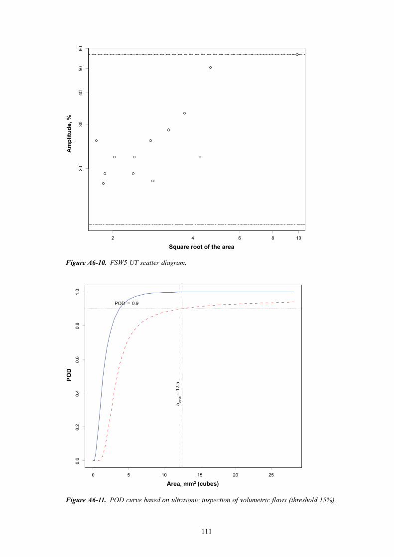
111

Figure A6-10. FSW5 UT scatter diagram.

Figure A6-11. POD curve based on ultrasonic inspection of volumetric flaws (threshold 15%).

2 4 6 8 10

2030

4050

60

Square root of the area

Am

plitu

de, %

0 5 10 15 20 25

0.0

0.2

0.4

0.6

0.8

1.0

Area, mm2 (cubes)

POD

POD = 0.9

a 90/9

5 = 1

2.5

112

A6.2.1.3 JLH

Figure A6-15 shows a typical cross section of a JLH (Joint Line Hooking) discontinuity. It is clear that this shape not easily matching the empirical POD approach. The investigation was refined step by step:The first approach in investigating the JLH flaws was just to apply the POD method in an empirical way. For â we applied the maximum echo amplitude as before. First a totally empirical “â versus a” scatter diagram and POD were created. These included all the values of the SKB experiments included which yields the a90/95 equal to the detectable radial dimension of 4.0... In the next step, outliers (too small and too big values compared to a “normal” amplitude versus size behaviour), were excluded. This resulted in detectable radial dimension is 3.2 mm due to the decreased scatter.

Figure A6-12. Critical region based on ultrasonic inspection of volumetric flaws (threshold 15%).

0 10 20 30 40 50

020

4060

8010

0

Radial size, mm (destr.)

Are

a, m

m2 (

cube

s)

a90/95 = 12.5 criti

cal s

ize

=35

a r=

6.3

Non−destr. inspection

Destructive inspection

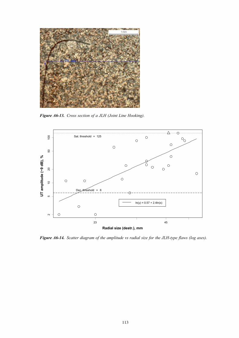
11�

Figure A6-13. Cross section of a JLH (Joint Line Hooking).

Figure A6-14. Scatter diagram of the amplitude vs radial size for the JLH-type flaws (log axes).

23 45

2

510

2050

100


UT

ampl

itude

(−9

dB),

%

ln(y) = 0.57 + 2.4ln(x)

Sat. threshold = 125

Dec. threshold = 6

114

Figure A6-15. POD curve for the JLH-type flaws (with outliers).

Figure A6-16. Scatter diagram of the amplitude vs radial size for the JLH-type flaws (log axes, without outliers).

0 2 4 6 8 10 12

0.0

0.2

0.4

0.6

0.8

1.0


POD

POD


PO D = 0.9

a 90/9

5 = 4

.0

1.5 2.0 2.5 3.0 3.5 4.0 4.5 5.0

2

510

2050

100


UT

ampl

itude

(−9

dB),

%

ln(y) = −0.0019 + 2.8ln(x)

Sat. threshold = 125

Dec. threshold = 6

11�

Figure A6-17. POD curve for the JLH-type flaws (outliers excluded).

0 2 4 6 8 10 12

0.0

0.2

0.4

0.6

0.8

1.0


POD

POD


POD = 0.9

a 90/9

5 = 3

.2

A6.3 Sizingcapabilities

In order to estimate the sizing capabilities of non-destructive testing, radial sizes of volu-metric and JLH-type flaws determined by means of radiographic and ultrasonic inspection have been compared with the corresponding values determined by destructive inspection.

A6.3.1 Methodology

Results have been summarized using box plots and a descriptive statistic that can be called “mean relative error”. Introductions of the box plot and the formula for the mean relative error is presented below.

Box plots /7/ provide a five-number summary for a set of observations. The summary consists of:• smallest observation,• 1st quartile, i.e. the observation that is larger than one quarter and smaller than three

quarters of all observations,• median, i.e. the observation that is larger than one half and smaller than the other half of

all observations,• 3rd quartile, i.e. the observation that is larger than three quarters and smaller than one

quarter of all observations,• largest observation.

Box plots provide an insight about the location and variation of the set of observations. We have used box plots to present the set of differences between measured and true (known from destructive testing) values of radial sizes. The results are given in the Section 7.2.

11�

Further, we summarized the differences for each non-destructive method using the “mean relative error” that has been calculated according to the formula (12).

(12)

The designations are as follows:

ST true radial size known from the destructive testingSE experimental (measured) radial sizeN number of observations

A6.3.2 Results

Figure A6-20 shows the box plot of the differences between the radial sizes of volumentric discontinuities measured by radiographic inspection (35°) and by destructive segmentation. It can be seen that:• all of the observed differences lie between –2.4 and 6.2 mm,• half of the observed differences lie between –1.2 mm (1st quartile) and 0.9 mm

(3rd quartile),• although the radial sizes of some discontinuities have been overestimated by as

much as 6 mm, the median difference value is negative (–0.2 mm), i.e. the trend is to underestimate the radial size.

Figure A6-21 shows the box plot of the differences between the radial sizes of volumentric discontinuities measured by ultrasonic inspection and by destructive segmentation. As shown in the figure,• all of the observed differences lie between –2.1 and 1.2 mm,• half of the observed differences lie between –1.6 mm (1st quartile) and –0.2 mm

(3rd quartile),• the ultrasonic testing tends to under-estimate radial sizes of discontinuities in the data

set under investigation (median difference value: –0.7 mm).

Figure A6-22 displays the box plot of the differences between the radial sizes of the JLH-type discontinuities measured by ultrasonic inspection and by destructive inspection. Apparently,• all of the observed differences lie between –1.4 and 2.5 mm,• half of the observed differences lie between –0.1 mm (1st quartile) and 1.1 mm

(3rd quartile).

The ultrasonic inspection tends to over-estimate the radial sizes of JLH-type flaws in the present data set (median value 0.5 mm). Nevertheless, there are some flaws that have been underestimated by as much as 1.4 mm presumably due to the fact that in the certain region of the flaw the surfaces get so tight that the flaw ceases to reflect ultrasound (kissing bonds).

11�

Figure A6-18. Box plot of the differences between the sizes for wormholes measured by radiographic inspection (35°) and destructive inspection in radial direction.

Figure A6-19. Box plot of the differences between the radial sizes for wormholes measured by ultrasonic inspection and destructive inspection.

−20

2

4

6

Rad

ial s

ize

(RT)

− R

adia

l siz

e (d

estr

.), m

m

−2.4

−1.2

−0.2

0.9

6.2

Smallest value

1st quartile

Median

3rd quartile

Largest value

−2.0

−1.0

0.0

0.5

1.0

Rad

ial s

ize

(UT)

− R

adia

l siz

e (d

estr

.), m

m

−2.1

−1.6

−0.7

−0.2

1.2

Smallest value

1st quartile

Median

3rd quartile

Largest value

11�

A7 SummaryofResults

A7.1 ProbabilityofDetection

Subject of consideration in this sub-report was the detectability of volumetric-like worm-holes and area-like “Joint line hooking” in friction stir welds with the SKB radiographic and ultrasonic methods. At the current state of the art all observed a90/95 values – as listened in Table A7-1 – are for the wormholes for radiographs not larger than 3 mm and for UT not larger than 13 mm2. The corresponding radial dimension are at maximum 4 mm for RT and 6.3 mm for UT in case the flaw configurations investigated here represent the full possible scale which might occur in the welds under production conditions. The empirical detectable radial dimension with UT for the “Joint line hooking” is 4 mm.

TableA7-1. SummaryofPODcurvesandcorrespondinga90/95andarvalues.

Identification Description a(independentvariable)

â(dependentvariable)

Decisionthreshold

a90/95 ar

Wormholes RT (standard threshold)

Based on measured contrast resulting from volumetric flaws

Penetrated size

Contrast 250 counts 2.60mm 4mm

Wormholes RT (standard threshold, corrected)

Based on meas. contrast resulting from vol. flaws and penetr. sizes measured destructively

Penetrated size (destr. testing)

Contrast 250 counts 0.97mm 2.4mm

Wormholes UT

Based on measured reflection from volumetric flaws

Area Echo height, % 15% 12.5mm2 6.3mm

JLH with “outliers”

Based on measured reflection from JLH-type flaws

Radial size Echo height, % 6% 4.0mm 4.0mm

JLH without “outliers”

Based on measured reflection from JLH-type flaws

Radial size Echo height, % 6% 3.2mm 3.2mm

Figure A6-20. Box plot of the differences between the radial sizes of the JLH-type flaws measured by ultrasonic inspection and by destructive inspection.

−10

1

2

Rad

. siz

e (U

T, −

6 dB

) − R

ad. s

ize

(des

tr.),

mm

−1.4

−0.1

0.5

1.1

2.5

Smallest value

1st quartile

Median

3rd quartile

Largest value

11�

A7.2 Sizingcapabilities

Overall results of the comparison are recapitulated in the Table A7-2.

TableA7-2. Summaryofsizingcapability.

Flawtype Inspectionmethod

Smallestdeviationofthemeasuredvaluefromthereferencevalue,mm

1stquartilemm

Mediandeviationofthemeasuredvaluefromthereferencevalue,mm

Meanrelativedeviation%

3rdquartilemm

Largestdeviationofthemeasuredvaluefromthereferencevalue,mm

Wormhole X-rays –2.4 –1.2 –0.2 3.7 0.9 6.2Wormhole Ultrasound –2.1 –1.6 –0.7 –16.2 –0.2 1.2

JLH Ultrasound –1.4 –0.1 0.5 26.1 1.1 2.5

RT of wormholes underestimates the size in radial direction. The underestimation might be due to the fact that the flaws become smaller towards the ends (as confirmed by the cross sections) decreasing the contrast. Basically the difference of radiation direction of 35° and the radial measurement of the flaw dimension makes the method dependent on the typical geometric distribution of the flaws. The wormholes belong more to the type of volumetric flaws and have in addition often a zig-zag shaped surface so that the sound is reflected in all possible directions which make an exact sizing by the 6 dB drop rule hard and the under-estimation understandable. The sizes of the JLHs are overestimated. They are in absolute value very small and might tend to the behaviour of a point reflector rather than a reflecting curved or flat plane.

A8 Conclusions

A Probability of Detection evaluation for the SKB-NDT processes has been successfully established to make sure the applied NDT techniques are able to reveal the occurring discontinuities and to quantify the discontinuity sizes, which might be overseen by NDT as an input for the final risk assessment. A generalization of the existing prescription for the signal response POD from the MIL 1823 standard was necessary because the FSW welds of 50 mm thick Cu-canister-welds are more complex than thin aerospace structures.

The physical reasonable a90/95 values as discontinuity sizes, which are detected for sure need to be set in correspondence to the corresponding radial dimensions of discontinuities to pro-vide the expected wall thickness reduction, which is of importance for the integrity require-ment. Subject of consideration for FSW was the detectability of volumetric like wormholes and area like “Joint line hooking” with the SKB radiographic and ultrasonic methods.

At the current state of the art all observed a90/95 values are for the wormholes for radiographs not larger than 3 mm and for UT not larger than 13 mm2. The corresponding radial dimen-sion are at maximum also 4 mm for RT and 6.3 mm for UT in case the flaw configurations investigated here represent the full possible scale which might occur in the welds under production conditions. The empirical detectable radial dimension with UT for the “joint line hooking” is 4 mm.

The sizing errors for both types of welds are for area like flaws of only a few millimeters using UT technique. Even for volumetric flaws, where UT is not so well suited, in FSW the absolute deviations are a couple of millimeters underestimation only. The joint line hooking discontinuities are overestimated even when there is a kissing part. All flaws are detected and sized with sufficient accuracy with respect to the intended purpose to avoid a critical flaw size of 35mm.

120

A9 References

/1/ BerensAP,1989. NDE reliability data analysis. In Metals Handbook, volume 17. ASM International, 9 edition.

/2/ USDepartmentofdefense,1999. Nondestructive evaluation system. Reliability assessment, 1999. Handbook.

/3/ ASTM. ASTM E1000, Chapter 11: Image Quality Considerations, p 438.

/4/ ASNT Nondestructive Testing Handbook, Second Edition, Volume 7: Ultrasonic Testing pp 445 (Factors Determining Amplitude of Discontinuity Echo Signal).

/5/ Non-Destructive Evaluation System Reliability Assessment, MIL-STD-1823 (U.S. Department of Defense).

/6/ Goebbels HECT.

/7/ ChambersJM,ClevelandWS,KleinerB,TukeyPA,1983. Graphical Methods for Data Analysis. Wadsworth & Brooks/Cole.

/8/ HaaseO,GoebbelsJ,IllerhausB,BaileyM,SenéM,1999. High Energy Tomography and Crack Dection, Proceedings of the Int. Symp. on Computerized Tomography for Indiustrial Applications and Image Processing in Radiology, March 15–17, 1999, Berlin, DGZfP Proceedings BB67-CD (1999), 233–239

/9/ MüllerC,etal.2006.Project NDT Reliability, final report,SKB R-06-08. Svensk Kärnbränslehantering AB.

A10 Abbreviations

a Defect Sizeâ Signal Magnitudea90/95 a at 90% Level of the 95% Confidence LimitASTM American Society for Testing of MaterialsBAM Bundesanstalt für Materialforschung und –prüfungCEN European Committee for StandardizationCS Contrast SensitivityCT Computerised TomographyCu CupperDDA Deutscher DampfkesselausschussDIN Deutsches Institut für Normung e.V.EBW Electron Beam WeldingEN European NormFBH Flat Bottom Holese. g. for ExampleFSW Friction steer WeldingHECT High Energy Computed TomographyIQI Image Quality IndicatorJLH Joint Line Hooking

121

MIL Military StandardNDE Nondestructive EvaluationNDT Nondestructive TestingPOD Probability of DetectionROC Receiver Operating CharacteristicRT Radiographic TestingSDD Source Detector DistanceSn TinSKB Svensk Kärnbränslehantering ABSNR signal/noise ratioTEK Technical ReportTWI The Welding InstituteUT Ultrasonic Testing

Reliability in sealing of canister for spent nuclear · PDF fileReliability in sealing of...

Documents

Transcript of Reliability in sealing of canister for spent nuclear · PDF fileReliability in sealing of...