Release 1.0 Hannah Lawrence - Read the Docs

sinctransform DocumentationRelease 1.0

Hannah Lawrence

Mar 22, 2019

Contents:

1 Overview 1

2 Package Contents 3

3 Installation and Usage 53.1 Configuration . . . . . . . . . . . . . . . . . . . . . . . . . . . . . . . . . . . . . . . . . . . . . . . 53.2 Testing . . . . . . . . . . . . . . . . . . . . . . . . . . . . . . . . . . . . . . . . . . . . . . . . . . 53.3 Usage . . . . . . . . . . . . . . . . . . . . . . . . . . . . . . . . . . . . . . . . . . . . . . . . . . . 5

4 Example Programs 7

5 Time and Performance Tests 9

6 Mathematical Derivation 116.1 Conventions . . . . . . . . . . . . . . . . . . . . . . . . . . . . . . . . . . . . . . . . . . . . . . . 116.2 Use of Convolution . . . . . . . . . . . . . . . . . . . . . . . . . . . . . . . . . . . . . . . . . . . . 126.3 Fourier Transform of Sinc . . . . . . . . . . . . . . . . . . . . . . . . . . . . . . . . . . . . . . . . 136.4 Fourier Transform of Sinc2 . . . . . . . . . . . . . . . . . . . . . . . . . . . . . . . . . . . . . . . 146.5 Implementation . . . . . . . . . . . . . . . . . . . . . . . . . . . . . . . . . . . . . . . . . . . . . . 15

7 Quadrature 177.1 Comparison of Methods . . . . . . . . . . . . . . . . . . . . . . . . . . . . . . . . . . . . . . . . . 177.2 Gauss-Legendre . . . . . . . . . . . . . . . . . . . . . . . . . . . . . . . . . . . . . . . . . . . . . 177.3 Modified Trapezoidal . . . . . . . . . . . . . . . . . . . . . . . . . . . . . . . . . . . . . . . . . . 18

8 Matlab 218.1 Instructions . . . . . . . . . . . . . . . . . . . . . . . . . . . . . . . . . . . . . . . . . . . . . . . . 218.2 Reconstruction Examples . . . . . . . . . . . . . . . . . . . . . . . . . . . . . . . . . . . . . . . . 21

9 Notes 239.1 FINUFFT . . . . . . . . . . . . . . . . . . . . . . . . . . . . . . . . . . . . . . . . . . . . . . . . . 239.2 Runtime . . . . . . . . . . . . . . . . . . . . . . . . . . . . . . . . . . . . . . . . . . . . . . . . . 239.3 Precision . . . . . . . . . . . . . . . . . . . . . . . . . . . . . . . . . . . . . . . . . . . . . . . . . 23

10 Citations and Licenses 2510.1 Relevant journal articles . . . . . . . . . . . . . . . . . . . . . . . . . . . . . . . . . . . . . . . . . 2510.2 Licenses . . . . . . . . . . . . . . . . . . . . . . . . . . . . . . . . . . . . . . . . . . . . . . . . . 26

i

CHAPTER 1

Overview

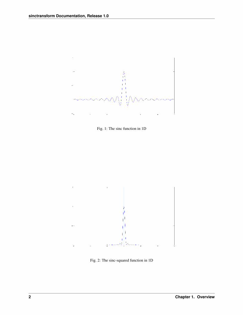
This is a C++ package to compute the sinc and sinc-squared transforms (based on [1]), defined as follows. Consider2𝑚 points in 𝑑 dimensional space, a1, ...,am,k1, ...,km ∈ R𝑑, with weights 𝑞1, ..., 𝑞𝑚 ∈ C. The task is to compute

𝑚∑︁𝑗=1

𝑞𝑗sinc(ai − kj) or𝑚∑︁𝑗=1

𝑞𝑗sinc2(ai − kj) for all 𝑖 = 1, . . . ,𝑚

where the 𝑑 dimensional sinc kernel is

sinc(x) =𝑑∏︁

𝑖=1

sin(𝑥𝑖)

𝑥𝑖x ∈ R𝑑

Sometimes, sinc is defined with an additional 𝜋 scaling, i.e. sinc(𝑥) = sin(𝜋𝑥)𝜋𝑥 . Our code has an option to specify

which convention you prefer.

The above task has naive complexity 𝑂(𝑚2). Our code uses a fast algorithm to compute it in 𝑂(𝑚 log 1/𝜖+𝐾𝑑 log𝐾)time, where 𝜖 > 0 is the desired relative tolerance, and 𝐾 is the maximal size of a cuboid containing the points (i.e.space-bandwidth product, or number of oscillations over such a cuboid).

Our code is in C++, handles 1, 2, and 3 dimensions, as well as the sinc2 kernel. It relies on the FIN-UFFT library to efficiently compute the type-3 nonuniform Fourier transform from the points to a set ofquadrature nodes for the Fourier transform of the kernel.

For completeness, there is also some MATLAB code to perform the same functions. The latter is slightly slower andnot as well-documented, but may be more convenient or easy to understand.

1

https://github.com/hannahlawrence/sinctransform

sinctransform Documentation, Release 1.0

Fig. 1: The sinc function in 1D

Fig. 2: The sinc-squared function in 1D

2 Chapter 1. Overview

CHAPTER 2

Package Contents

The sinc and sinc-squared transform of specified dimension:

sinc1d.cppsinc2d.cppsinc3d.cppsinctransform.hpp

To compute the sinc transform directly:

directsinc.cppdirectsinc.hpp

Programs used in directsinc.cpp, as well as all example and testing code, to print arrays, generate random arrays, etc:

sincutil.cppsincutil.hpp

For computing Gauss-Legendre quadrature nodes and weights (see [2] in citations):

fastGL.cppfastGL.hpp

Simple usage examples for specified dimension:

example1d.cppexample2d.cppexample3d.cpp

Accuracy testing at precision range for specified dimension:

test1d.cpptest2d.cpptest3d.cpp

Matlab code (not C++ wrappers) for sinc transform:

3


sinc1d.msinc2d.msinc3d.msincsq1d.msincsq2d.msincsq3d.m

Matlab file containing precomputed constants for trapezoidal constants:

newconstants.mat

Matlab to compute Gauss-Legendre nodes and weights, and to generate a 3d Shepp-Logan phantom (credit to Gregvon Winckel and Matthias Schabel, respectively; see licenses):

lgwt.mphantom3d.m

As one application-based example, we also include annotated Matlab code to reconstruct an image from its nonuni-formly sampled Fourier data, using the autoquad and sinc functions:

recon2d.mrecon3d.m

These use the following to compute the “optimal” quadrature weights for reconstruction, as described in [1] of cita-tions, via the sinc-squared programs:

autoquad1d.mautoquad2d.mautoquad3d.m

4 Chapter 2. Package Contents

CHAPTER 3

Installation and Usage

1. Install the finufft library, including all of its required libraries

2. Download contents of sinctransform package, i.e. “git clone https://github.com/hannahlawrence/sinctransform.git”

3.1 Configuration

1. In the makefile, change FINUFFT to the path to finufft:

FINUFFT = /some/path/to/finufft

1. In the makefile, change FFTW to the directory containing the fftw library:

FFTW = /some/path/to/fft

(Note: on a Mac, this may be /usr/local/lib. On linux it is /usr/lib/x86_64-linux-gnu)

3.2 Testing

Run make all to build and test the library. All tests and examples should complete without error. The tests should runfor less than 30 seconds.

3.3 Usage

To use in other programs, begin by creating the static library:

make lib

This creates libsinc.a, which should be linked against your code. In your code, make sure to include the header file:

5

https://github.com/ahbarnett/finufft

https://github.com/hannahlawrence/sinctransform.git

https://github.com/hannahlawrence/sinctransform.git


#include "sinctransform.hpp"

The sinc functions also expect a complex<double> array for q (even if all the complex values are 0), so it will also benecessary to include the corresponding header:

#include <complex>

Then compile with both the sinctransform and finufft static libraries, e.g.

g++ -std=c++11 -Wall -g -o myprog myprog.cpp /path/to/libsinc.a /path/to/finufft/lib/→˓libfinufft.a -lfftw3 -lm

It may be necessary to include a flag telling the compiler where to find the FFTW library, which is a prerequisite forthe finufft library. To do so, add the flag “-L/some/dir” such that /some/dir contains the static FFTW library (.a file, inlib-static directory of finufft library).

6 Chapter 3. Installation and Usage

CHAPTER 4

Example Programs

Some very simple usage examples in 1D, 2D, and 3D are contained within the examples directory. They also checkaccuracy of the result. To run:

make examples

examples/example1dexamples/example2dexamples/example3d

It is also possible to make and run all examples simultaneously:

make examples

7


8 Chapter 4. Example Programs

CHAPTER 5

Time and Performance Tests

Test scripts in 1D, 2D, and 3D are included in the test directory. They compare running time of the sinc and sincsqprograms to the brute force approach. In addition, accuracy is measured by the L2 error with respect to the result of thedirect calculation. To enable larger-scale testing, on which the complete direct computation becomes intractable, theL2 error is approximated by the L2 error of a tractable subset of the requested outputs, as determined by the “numeval”variable.

To run:

make tests/test2dtests/test2d

It is also possible to make and run all tests simultaneously:

make tests

9


10 Chapter 5. Time and Performance Tests

CHAPTER 6

Mathematical Derivation

Recall the objective is to compute, for all 𝑖 = 1, . . .𝑚,

𝑚∑︁𝑗=1

𝑞𝑗sinc(ai − kj)

𝑚∑︁𝑗=1

𝑞𝑗sinc2(ai − kj)

We will exploit the fact that the the FINUFFT library quickly computes expressions of the form

𝑚∑︁𝑗=1

𝑓(𝑥𝑗)𝑒±𝑖𝑥𝑗𝑘𝑟 for all 𝑟 = 1, . . . , 𝑛

much faster than the naive 𝑂(𝑛𝑚) time, where the points 𝑥𝑗 and 𝑘𝑟 may be arbitrarily spaced.

6.1 Conventions

ℱ(ℎ(x))(f) =

∫︁ ∞

−∞ℎ(x)𝑒−2𝜋𝑖xf𝑑𝑥

ℱ−1(𝐻(f))(x) =

∫︁ ∞

−∞𝐻(f)𝑒2𝜋𝑖xf𝑑𝑓

sinc(𝑥) =sin(𝑥)

𝑥sinc(x) = sinc(𝑥1)sinc(𝑥2)sinc(𝑥3)

Note that sometimes sinc(𝑥) is defined as sin(𝜋𝑥)𝜋𝑥 . The derivation below is the same, with some minor alterations to

constants. This option is included in the code, as the ifl flag.

11


6.2 Use of Convolution

Define

𝑓(k) =

𝑚∑︁𝑗=1

𝛿(k− kj)𝑞𝑗

Fig. 1: One example of 𝑓 , where the y-axis measures area

ℱ(𝑓(k)) =

∫︁ ∞

−∞

𝑚∑︁𝑗=1

𝛿(k− kj)𝑞𝑗𝑒−2𝜋𝑖kx𝑑k =

𝑚∑︁𝑗=1

𝑞𝑗𝑒−2𝜋𝑖kjx

Then

(sinc * 𝑓)(ai) =∫︁ ∞

−∞sinc(ai − k)𝑓(k)𝑑k

=

𝑚∑︁𝑗=1

𝑞𝑗

∫︁ ∞

−∞sinc(ai − k)𝛿(k− kj)𝑑k

=

𝑚∑︁𝑗=1

𝑞𝑗sinc(ai − kj)

Similarly

(sinc2 * 𝑓)(ai) =∫︁ ∞

−∞sinc2(ai − k)𝑓(k)𝑑k

=

𝑚∑︁𝑗=1

𝑞𝑗

∫︁ ∞

−∞sinc2(ai − k)𝛿(k− kj)𝑑k

=

𝑚∑︁𝑗=1

𝑞𝑗sinc2(ai − kj)

So, the desired quantities are (sinc * 𝑓)(ai) and (sinc2 * 𝑓)(ai). But by the convolution theorem:

(sinc * 𝑓)(ai) = ℱ−1(ℱ(sinc)ℱ(𝑓))(ai)

(sinc2 * 𝑓)(ai) = ℱ−1(ℱ(sinc2)ℱ(𝑓))(ai)

Luckily, ℱ(sinc) and ℱ(sinc2) take simple forms, which are derived below.

12 Chapter 6. Mathematical Derivation


6.3 Fourier Transform of Sinc

6.3.1 1D

Consider the function

ℎ(𝑥) = 𝑏 |𝑥| ≤ 𝑎

0 |𝑥| > 𝑎

We have that

ℱ(ℎ(𝑥))(𝑓) =

∫︁ 𝑎

−𝑎

𝑏𝑒−2𝜋𝑖𝑥𝑓𝑑𝑥 = 2𝑎𝑏sinc(2𝜋𝑎𝑓)

Using the symmetry of Fourier transform, i.e. ℱ(ℎ(𝑥))(𝑓) = ℎ(−𝑓), and that ℎ(𝑥) is even:

ℱ(𝐻(𝑥))(𝑓) = ℱ(2𝑎𝑏sinc(2𝜋𝑎𝑥))(𝑓) = ℎ(𝑥)

Then ℎ(𝑥) with 𝑎 = 12𝜋 and 𝑏 = 𝜋 is equal to ℱ(sinc(𝑥))(𝑓), as shown below.

Fig. 2: The Fourier transform of sinc in 1D.

6.3.2 2D

Again, let

ℎ(𝑥) = 𝑏 𝑥1 ≤ 𝑎, 𝑥2 ≤ 𝑎

0 𝑥1 > 𝑎, 𝑥2 > 𝑎

ℱ(ℎ(x))(f) =

∫︁ 𝑎

−𝑎

∫︁ 𝑎

−𝑎

𝑏𝑒−2𝜋𝑖xf𝑑x = 4𝑎2𝑏sinc(2𝜋𝑎𝑓1)sinc(2𝜋𝑎𝑓2) = 4𝑎2𝑏sinc(2𝜋𝑎f)

As before, setting 𝑎 = 12𝜋 and 𝑏 = 𝜋2 yields ℱ(sinc(x))(𝑓)

6.3.3 3D

Let

ℎ(𝑥) = 𝑏 𝑥1 ≤ 𝑎, 𝑥2 ≤ 𝑎, 𝑥3 ≤ 𝑎

0 𝑥1 > 𝑎, 𝑥2 > 𝑎, 𝑥3 > 𝑎

6.3. Fourier Transform of Sinc 13


ℱ(ℎ(x))(f) =

∫︁ 𝑎

−𝑎

∫︁ 𝑎

−𝑎

∫︁ 𝑎

−𝑎

𝑏𝑒−2𝜋𝑖xf𝑑x = 8𝑎3𝑏sinc(2𝜋𝑎𝑓1)sinc(2𝜋𝑎𝑓2)sinc(2𝜋𝑎𝑓3) = 8𝑎3𝑏sinc(2𝜋𝑎f)

Setting 𝑎 = 12𝜋 and 𝑏 = 𝜋3 yields ℱ(sinc(x))(𝑓)

6.4 Fourier Transform of Sinc2

The following basic fact about convolution, combined with the previous section, will easily provide the Fourier trans-form of sinc2

ℱ(sinc2(x))(f) = (ℱ(sinc(x)) * ℱ(sinc(x)))(f)

6.4.1 1D

ℱ(sinc2(x))(f) = 𝜋(1− 𝜋|𝑥|) |𝑥| ≤ 1

𝜋

0 |𝑥| > 1

𝜋

Fig. 3: The Fourier transform of sinc-squared in 1D.

6.4.2 2D

ℱ(sinc2(x))(f) = 𝜋2(1− 𝜋|𝑥1|)(1− 𝜋|𝑥2|) |𝑥1| ≤1

𝜋, |𝑥2| ≤

1

𝜋

0 |𝑥1| >1

𝜋, |𝑥2| >

1

𝜋



6.4.3 3D

ℱ(sinc2(x))(f) = 𝜋2(1− 𝜋|𝑥1|)(1− 𝜋|𝑥2|)(1− 𝜋|𝑥3|) |𝑥1| ≤1

𝜋, |𝑥2| ≤

1

𝜋, |𝑥3| ≤

1

𝜋

0 |𝑥1| >1

𝜋, |𝑥2| >

1

𝜋, |𝑥3| >

1

𝜋

6.5 Implementation

Putting together the previous sections:

(sinc * 𝑓)(ki) = ℱ−1(ℱ(sinc)ℱ(𝑓))(ki)

=

∫︁ 12𝜋

−12𝜋

𝜋(︁ 𝑚∑︁

𝑗=1

𝑞𝑗𝑒−2𝜋𝑖𝑘𝑗𝑥

)︁𝑒2𝜋𝑖𝑥𝑘𝑖𝑑𝑥

=1

2

∫︁ 1

−1

(︁ 𝑚∑︁𝑗=1

𝑞𝑗𝑒−𝑖𝑘𝑗𝑦

)︁𝑒𝑖𝑦𝑘𝑖𝑑𝑦

In 2 and 3 dimensions, the constant 12 changes to 1

4 and 18 , respectively, and integration is multidimensional with the

same bounds.

(sinc2 * 𝑓)(ki) = ℱ−1(ℱ(sinc2)ℱ(𝑓))(ki)

=

∫︁ 1𝜋

−1𝜋

𝜋(1− 𝜋|𝑥|)(︁ 𝑚∑︁

𝑗=1

𝑞𝑗𝑒−2𝜋𝑖𝑘𝑗𝑥

)︁𝑒2𝜋𝑖𝑥𝑘𝑖𝑑𝑥

=1

4

∫︁ 2

−2

(2− |𝑦|)(︁ 𝑚∑︁

𝑗=1

𝑞𝑗𝑒−𝑖𝑘𝑗𝑦

)︁𝑒𝑖𝑦𝑘𝑖𝑑𝑦

Again, in 2 and 3 dimensions, the constant 14 changes to 1

8 and 116 , respectively, and integration is multidimensional.

In each case, there are two main tasks: computing the inner summation, and computing the outer (possibly multidi-mensional) integral. But the inner summation is exactly a discrete (nonuniform) Fourier transform, and is computedwith the finufft library. The outer integral again takes the form of of a Fourier transform (in the other direction), butsince we want the exact integral, quadrature weights (either Gauss-Legendre of corrected trapezoidal, from Kapur-Rokhlin) are used to weight the integrand before again applying the finufft library. Note that in the case of sinc2, theintegrand is only piecewise continuous, so the quadrature points are treated accordingly.

6.5. Implementation 15

CHAPTER 7

Quadrature

There are two built-in quadrature options when approximating the final integral (see Derivation page): Gauss-Legendre[2], and corrected trapezoidal quadrature [3]. The choice is specified by the “quad” input parameter to each functon.The corrected trapezoidal rule is faster, particularly for inputs requiring many quadrature points (i.e. with high-valued𝑘𝑖 or 𝑎𝑖) with high requested precision, and is thus recommended.

7.1 Comparison of Methods

The accuracy and computation of the two quadrature methods is dependent on many factors, including 𝑁 and thenumber of quadrature points (affected by the maximum excursion of 𝑘𝑖 and 𝑎𝑖). This is one example of 3D sinc inwhich there are many quadrature points, and so the trapezoidal quadrature has a significant advantage.

Fig. 1: Oversampling parameter and number of corrections for corrected trapezoidal quadrature. max |𝑘𝑖| = 50

7.2 Gauss-Legendre

The default upsampling parameter for the number of quadrature points, 𝑟𝑠𝑎𝑚𝑝, is set to 2. This can be modifieddirectly within the functions as required. The effect of this parameter on the precision accuracy, and computation

17


time, is shown below. Unsurprisingly, a higher upsampling parameter can at first improve accuracy somewhat, buteventually flatlines. It consistently increases computation time.

Fig. 2: Effect of oversampling parameter for Gauss-Legendre quadrature, 1D sinc. max 𝑎𝑖 ≤ 1000𝜋


7.3 Modified Trapezoidal

The default upsampling parameter for the number of regular trapezoidal quadrature points, 𝑟𝑠𝑎𝑚𝑝, is set to 3, based onthe empirical results below. There is an additional parameter corresponding to the number of correction terms, 𝑒. Theconstants are included for 𝑒 between 1 and 60, which thus restricts the allowable values of 𝑒. By default, it is set to 25,based again on the tests below. This can be modified directly within the functions as required. The interplay betweenthese two parameters is shown below. Once again, higher values for both parameters can improve accuracy to a certaindegree. The computation time is dominated by the nonuniform Fourier transforms. In this example, computation timeincreases with rsamp but is largely independent of 𝑒 when there are many quadrature points. With fewer quadraturepoints, there is greater dependence on 𝑒

18 Chapter 7. Quadrature



Fig. 5: Effect of oversampling parameter and number of corrections for corrected trapezoidal quadrature, 1D sinc.max 𝑎𝑖 ≤ 1000𝜋


7.3. Modified Trapezoidal 19



20 Chapter 7. Quadrature

CHAPTER 8

Matlab

8.1 Instructions

The test codes are built into the matlab files themselves, in the form of self-contained test and direct calculationfunctions near the end of each file. To run, simply call the function without any input arguments. The test functionsalso demonstrate appropriate usage, which is more straightforward than in C++. The input vectors can be modified todetermine what input precision is appropriate for a particular regime.

Note that the programs are self-contained – they are not Matlab interfaces to the C++, but pure Matlab code. As such,the only setup step is to ensure the FINUFFT matlab interfaces are on the matlab path.

To use the FINUFFT Matlab interfaces, follow their documentation. Then, use Matlab’s “addpath” to ensure theFINUFFT programs (e.g. finufft2d3) will be found.

http://finufft.readthedocs.io/en/latest/index.html

Finally, make sure lgwt.m is in the same directory, or that its directory is also included in Matlab’s path.

8.2 Reconstruction Examples

In the recon directory, the autoquad functions will compute quadrature weights based on the coordinates sampledin k-space (see [1]). recon2d.m and recon3d.m use these weights in several different ways to reconstruct simulateddata (the Shepp-Logan phantom). Note that recon3d is still under development, as autoquad3d can handle only smallnumbers of samples in a reasonable amount of time.

If using the recon examples from within the recon directory, also ensure that the directory one level above (containingall the sinc programs) is on Matlab’s path.

21

http://finufft.readthedocs.io/en/latest/index.html


22 Chapter 8. Matlab

CHAPTER 9

Notes

9.1 FINUFFT

The current installation instructions do not use the parallel capability of FINUFFT, which would provide an additionalspeedup. To do so, follow the installation instructions of FINUFFT regarding the openmp library and the appropriatecompilation flags.

9.2 Runtime

The code presented here scales much better than direct calculation (one can experiment with the tests directory toverify this). However, note that the runtime is heavily dependent on the speed of the nonuniform Fourier transforms,which in turn depend on a variety of factors.

9.3 Precision

The requested precision is not guaranteed, so it may be worth running a few test cases in the same regime (size andscale) as the intended application to pin down the optimal input precision. When necessary, it is also possible to changesome of the default parameters, depending on choice of quadrature, to achieve better precision; see the Quadraturepage for details.

23


24 Chapter 9. Notes

CHAPTER 10

Citations and Licenses

Main author of sinctransform: Hannah Lawrence.

sinctranform was written while Hannah was a summer intern at the Numerical Algorithms Group, Center for Compu-tational Biology, Flatiron Institute, NYC.

Collaborators: Leslie Greengard, Alex Barnett, Jeremy Magland (Flatiron Institute)

10.1 Relevant journal articles

Sinc transform:

[1] Greengard, L., Lee, J-Y., & Inati, S. (2006). The fast sinc transform and image reconstruction from non-uniformsamples in k-space, Communications in Applied Mathematics and Computational Science, 1, 121-132.

Computation of Gauss-Legendre quadrature weights via fastGL.cpp and fastGL.hpp:

[2] Ignace Bogaert, Iteration-free computation of Gauss-Legendre quadrature nodes and weights, SIAM Journal onScientific Computing, Volume 36, Number 3, 2014, pages A1008-1026.

Corrected trapezoidal quadrature weights:

[3] Sharad Kapur & Vladimir Rokhlin (1997). High-Order Corrected Trapezoidal Quadrature Rules for SingularFunctions, SIAM Journal of Numerical Analysis, Vol. 34, No. 4, pp. 1331–1356

FINUFFT library:

[4] (coming soon)

3d k-space sampling (for 3d reconstruction example):

[5] Park J, Shin T, Yoon SH, Goo JM, Park J-Y. A radial sampling strategy for uniform k-space coverage with ret-rospective respiratory gating in 3D ultrashort-echo-time lung imaging. NMR in biomedicine. 2016;29(5):576-587.doi:10.1002/nbm.3494.

25


10.2 Licenses

10.2.1 Sinc and FINUFFT

Copyright (C) 2017-2018 The Simons Foundation, Inc. - All Rights Reserved.

Main author: Hannah Lawrence.

In collaboration with: Leslie Greengard, Alex Barnett, Jeremy Magland (Flatiron Institute)

sinctransform is licensed under the Apache License, Version 2.0 (the “License”); you may not use this file except incompliance with the License. You may obtain a copy of the License at

http://www.apache.org/licenses/LICENSE-2.0

Unless required by applicable law or agreed to in writing, software distributed under the License is distributed on an“AS IS” BASIS, WITHOUT WARRANTIES OR CONDITIONS OF ANY KIND, either express or implied. See theLicense for the specific language governing permissions and limitations under the License.

10.2.2 C++ functions for Gauss-Legendre quadrature

Code based on [2], by J. Burkardt. Code distributed under the BSD license, which can be found at

https://people.sc.fsu.edu/~jburkardt/txt/bsd_license.txt

10.2.3 3d phantom

From MathWorks File Exchange, via BSD license (see above)

10.2.4 Matlab functions for Gauss-Legendre quadrature

Copyright (c) 2009, Greg von Winckel All rights reserved.

Redistribution and use in source and binary forms, with or without modification, are permitted provided that thefollowing conditions are met:

• Redistributions of source code must retain the above copyright notice, this list of conditions and the followingdisclaimer.

• Redistributions in binary form must reproduce the above copyright notice, this list of conditions and the follow-ing disclaimer in the documentation and/or other materials provided with the distribution.

THIS SOFTWARE IS PROVIDED BY THE COPYRIGHT HOLDERS AND CONTRIBUTORS “AS IS” AND ANYEXPRESS OR IMPLIED WARRANTIES, INCLUDING, BUT NOT LIMITED TO, THE IMPLIED WARRANTIESOF MERCHANTABILITY AND FITNESS FOR A PARTICULAR PURPOSE ARE DISCLAIMED. IN NO EVENTSHALL THE COPYRIGHT OWNER OR CONTRIBUTORS BE LIABLE FOR ANY DIRECT, INDIRECT, IN-CIDENTAL, SPECIAL, EXEMPLARY, OR CONSEQUENTIAL DAMAGES (INCLUDING, BUT NOT LIMITEDTO, PROCUREMENT OF SUBSTITUTE GOODS OR SERVICES; LOSS OF USE, DATA, OR PROFITS; OR BUSI-NESS INTERRUPTION) HOWEVER CAUSED AND ON ANY THEORY OF LIABILITY, WHETHER IN CON-TRACT, STRICT LIABILITY, OR TORT (INCLUDING NEGLIGENCE OR OTHERWISE) ARISING IN ANYWAY OUT OF THE USE OF THIS SOFTWARE, EVEN IF ADVISED OF THE POSSIBILITY OF SUCH DAM-AGE.

26 Chapter 10. Citations and Licenses

http://www.apache.org/licenses/LICENSE-2.0

https://people.sc.fsu.edu/~jburkardt/txt/bsd_license.txt

Release 1.0 Hannah Lawrence - Read the Docs

Documents

Transcript of Release 1.0 Hannah Lawrence - Read the Docs