Relativity in the Global Positioning System -...

Relativity in the Global Positioning System

Neil AshbyDept. of Physics, University of Colorado

Boulder, CO 80309–0390U.S.A.

[email protected]://physics.colorado.edu/faculty/ashby_n.html

Published on 28 January 2003

www.livingreviews.org/Articles/Volume6/2003-1ashby

Living Reviews in RelativityPublished by the Max Planck Institute for Gravitational Physics

Albert Einstein Institute, Germany

Abstract

The Global Positioning System (GPS) uses accurate, stable atomicclocks in satellites and on the ground to provide world-wide position andtime determination. These clocks have gravitational and motional fre-quency shifts which are so large that, without carefully accounting fornumerous relativistic effects, the system would not work. This paper dis-cusses the conceptual basis, founded on special and general relativity, fornavigation using GPS. Relativistic principles and effects which must beconsidered include the constancy of the speed of light, the equivalenceprinciple, the Sagnac effect, time dilation, gravitational frequency shifts,and relativity of synchronization. Experimental tests of relativity ob-tained with a GPS receiver aboard the TOPEX/POSEIDON satellite willbe discussed. Recently frequency jumps arising from satellite orbit adjust-ments have been identified as relativistic effects. These will be explainedand some interesting applications of GPS will be discussed.

c©2003 Max-Planck-Gesellschaft and the authors. Further information oncopyright is given at http://www.livingreviews.org/Info/Copyright/. Forpermission to reproduce the article please contact [email protected].

http://physics.colorado.edu/faculty/ashby_n.html

http://www.livingreviews.org/Info/Copyright/.

Article Amendments

On author request a Living Reviews article can be amended to include errataand small additions to ensure that the most accurate and up-to-date informa-tion possible is provided. For detailed documentation of amendments, pleasego to the article’s online version at

http://www.livingreviews.org/Articles/Volume6/2003-1ashby/.

Owing to the fact that a Living Reviews article can evolve over time, we rec-ommend to cite the article as follows:

Ashby, N.,“Relativity in the Global Positioning System”,

Living Rev. Relativity, 6, (2003), 1. [Online Article]: cited on <date>,http://www.livingreviews.org/Articles/Volume6/2003-1ashby/.

The date in ’cited on <date>’ then uniquely identifies the version of the articleyou are referring to.

http://www.livingreviews.org/Articles/Volume6/2003-1ashby/.

3 Relativity in the Global Positioning System

Contents

1 Introduction 4

2 Reference Frames and the Sagnac Effect 7

3 GPS Coordinate Time and TAI 11

4 The Realization of Coordinate Time 15

5 Relativistic Effects on Satellite Clocks 17

6 TOPEX/POSEIDON Relativity Experiment 22

7 Doppler Effect 26

8 Crosslink Ranging 28

9 Frequency Shifts Induced by Orbit Changes 30

10 Secondary Relativistic Effects 40

11 Applications 42

12 Conclusions 43

References 44

Living Reviews in Relativity (2003-1)http://www.livingreviews.org

http://www.livingreviews.org

N. Ashby 4

1 Introduction

The Global Positioning System (GPS) can be described in terms of three princi-pal “segments”: a Space Segment, a Control Segment, and a User Segment. TheSpace Segment consists essentially of 24 satellites carrying atomic clocks. (Sparesatellites and spare clocks in satellites exist.) There are four satellites in each ofsix orbital planes inclined at 55 with respect to earth’s equatorial plane, dis-tributed so that from any point on the earth, four or more satellites are almostalways above the local horizon. Tied to the clocks are timing signals that aretransmitted from each satellite. These can be thought of as sequences of eventsin spacetime, characterized by positions and times of transmission. Associatedwith these events are messages specifying the transmission events’ spacetimecoordinates; below I will discuss the system of reference in which these coordi-nates are given. Additional information contained in the messages includes analmanac for the entire satellite constellation, information about satellite vehiclehealth, and information from which Universal Coordinated Time as maintainedby the U.S. Naval Observatory – UTC(USNO) – can be determined.

The Control Segment is comprised of a number of ground-based monitoringstations, which continually gather information from the satellites. These dataare sent to a Master Control Station in Colorado Springs, CO, which analyzesthe constellation and projects the satellite ephemerides and clock behaviourforward for the next few hours. This information is then uploaded into thesatellites for retransmission to users.

The User Segment consists of all users who, by receiving signals transmittedfrom the satellites, are able to determine their position, velocity, and the timeon their local clocks.

The GPS is a navigation and timing system that is operated by the UnitedStates Department of Defense (DoD), and therefore has a number of aspects toit that are classified. Several organizations monitor GPS signals independentlyand provide services from which satellite ephemerides and clock behavior can beobtained. Accuracies in the neighborhood of 5–10 cm are not unusual. Carrierphase measurements of the transmitted signals are commonly done to betterthan a millimeter.

GPS signals are received on earth at two carrier frequencies, L1 (154 ×10.23 MHz) and L2 (120×10.23 MHz). The L1 carrier is modulated by two typesof pseudorandom noise codes, one at 1.023 MHz – called the Coarse/Acquisitionor C/A-code – and an encrypted one at 10.23 MHz called the P-code. P-code receivers have access to both L1 and L2 frequencies and can correct forionospheric delays, whereas civilian users only have access to the C/A-code.There are thus two levels of positioning service available in real time, the PrecisePositioning Service utilizing P-code, and the Standard Positioning Service usingonly C/A-code. The DoD has the capability of dithering the transmitted signalfrequencies and other signal characteristics, so that C/A-code users would belimited in positioning accuracy to about ±100 meters. This is termed SelectiveAvailability, or SA. SA was turned off by order of President Clinton in May,2000.




0 2 4 6 8-16

-15

-14

-13

-12

-11

-10

Log10( τ )

Quartz

CesiumLog10[ σy( τ ) ]

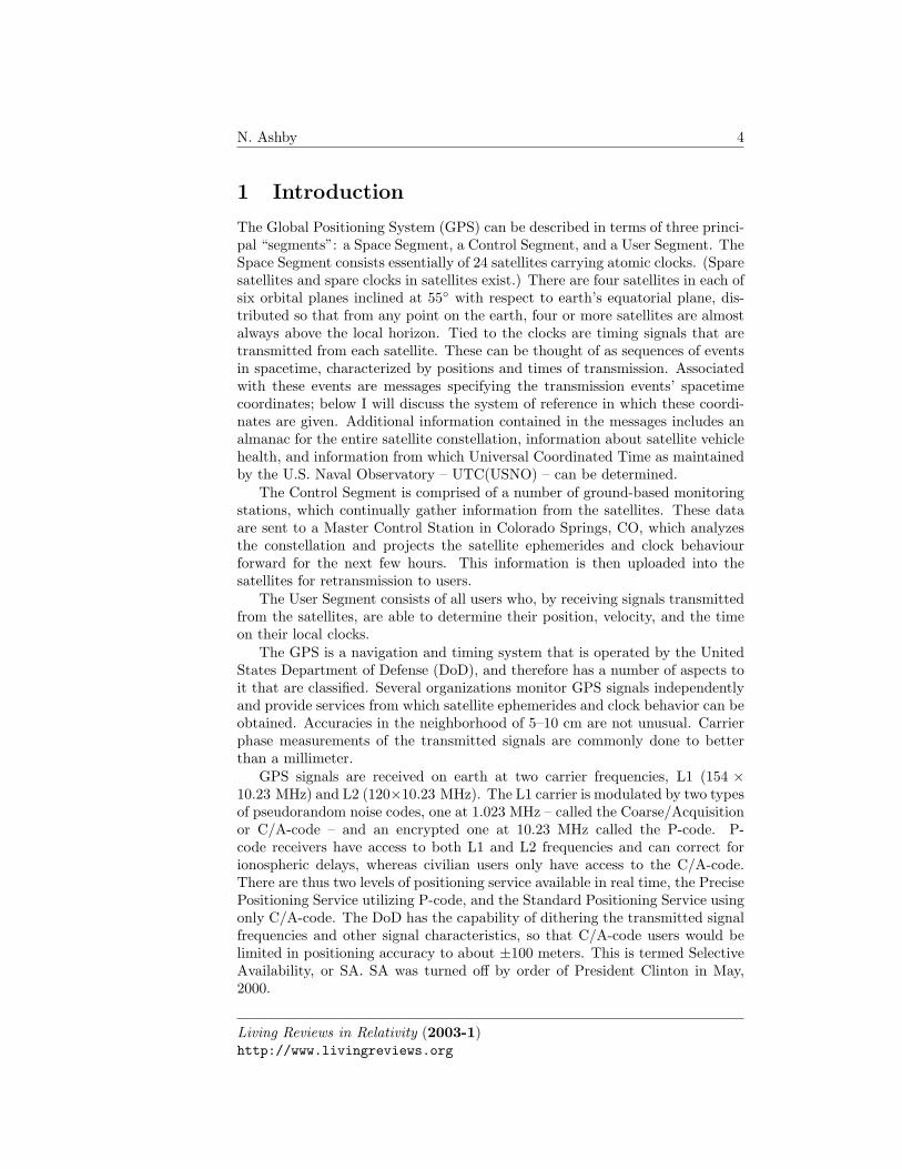
Figure 1: Typical Allan deviations of Cesium clocks and quartz oscillators, plot-ted as a function of averaging time τ .

The technological basis for GPS lies in extremely accurate, stable atomicclocks. Figure 1 gives a plot of the Allan deviation for a high-performanceCesium clock, as a function of sample time τ . If an ensemble of clocks is initiallysynchronized, then when compared to each other after a time τ , the Allandeviation provides a measure of the rms fractional frequency deviation amongthe clocks due to intrinsic noise processes in the clocks. Frequency offsets andfrequency drifts are additional systematic effects which must be accounted forseparately. Also on Figure 1 is an Allan deviation plot for a Quartz oscillatorsuch as is typically found in a GPS receiver. Quartz oscillators usually havebetter short-term stability performance characteristics than Cesium clocks, butafter 100 seconds or so, Cesium has far better performance. In actual clocksthere is a wide range of variation around the nominal values plotted in Figure 1.

The plot for Cesium, however, characterizes the best orbiting clocks in theGPS system. What this means is that after initializing a Cesium clock, andleaving it alone for a day, it should be correct to within about 5 parts in 1014,or 4 nanoseconds. Relativistic effects are huge compared to this.

The purpose of this article is to explain how relativistic effects are accountedfor in the GPS. Although clock velocities are small and gravitational fields areweak near the earth, they give rise to significant relativistic effects. These effectsinclude first- and second-order Doppler frequency shifts of clocks due to theirrelative motion, gravitational frequency shifts, and the Sagnac effect due toearth’s rotation. If such effects are not accounted for properly, unacceptablylarge errors in GPS navigation and time transfer will result. In the GPS onecan find many examples of the application of fundamental relativity principles.



N. Ashby 6

These are worth careful study. Also, experimental tests of relativity can beperformed with GPS, although generally speaking these are not at a level ofprecision any better than previously existing tests.

The principles of position determination and time transfer in the GPS can bevery simply stated. Let there be four synchronized atomic clocks that transmitsharply defined pulses from the positions rj at times tj , with j = 1, 2, 3, 4 anindex labelling the different transmission events. Suppose that these four signalsare received at position r at one and the same instant t. Then, from the principleof the constancy of the speed of light,

c2(t− tj)2 = |r− rj |2, j = 1, 2, 3, 4. (1)

where the defined value of c is exactly 299792458 m s−1. These four equationscan be solved for the unknown space-time coordinates r, t of the receptionevent. Hence, the principle of the constancy of c finds application as the funda-mental concept on which the GPS is based. Timing errors of one ns will lead topositioning errors of the order of 30 cm. Also, obviously, it is necessary to specifycarefully the reference frame in which the transmitter clocks are synchronized,so that Eq. (1) is valid.

The timing pulses in question can be thought of as places in the transmittedwave trains where there is a particular phase reversal of the circularly polarizedelectromagnetic signals. At such places the electromagnetic field tensor passesthrough zero and therefore provides relatively moving observers with sequencesof events that they can agree on, at least in principle.




2 Reference Frames and the Sagnac Effect

Almost all users of GPS are at fixed locations on the rotating earth, or else aremoving very slowly over earth’s surface. This led to an early design decision tobroadcast the satellite ephemerides in a model earth-centered, earth-fixed, ref-erence frame (ECEF frame), in which the model earth rotates about a fixed axiswith a defined rotation rate, ωE = 7.2921151467× 10−5 rad s−1. This referenceframe is designated by the symbol WGS-84(G873) [19, 3]. For discussions ofrelativity, the particular choice of ECEF frame is immaterial. Also, the fact thethe earth truly rotates about a slightly different axis with a variable rotationrate has little consequence for relativity and I shall not go into this here. I shallsimply regard the ECEF frame of GPS as closely related to, or determined by,the International Terrestrial Reference Frame established by the BIPM.

It should be emphasized that the transmitted navigation messages providethe user only with a function from which the satellite position can be calculatedin the ECEF as a function of the transmission time. Usually, the satellitetransmission times tj are unequal, so the coordinate system in which the satellitepositions are specified changes orientation from one measurement to the next.Therefore, to implement Eqs. (1), the receiver must generally perform a differentrotation for each measurement made, into some common inertial frame, so thatEqs. (1) apply. After solving the propagation delay equations, a final rotationmust usually be performed into the ECEF to determine the receiver’s position.This can become exceedingly complicated and confusing. A technical note [10]discusses these issues in considerable detail.

Although the ECEF frame is of primary interest for navigation, many physi-cal processes (such as electromagnetic wave propagation) are simpler to describein an inertial reference frame. Certainly, inertial reference frames are neededto express Eqs. (1), whereas it would lead to serious error to assert Eqs. (1)in the ECEF frame. A “Conventional Inertial Frame” is frequently discussed,whose origin coincides with earth’s center of mass, which is in free fall with theearth in the gravitational fields of other solar system bodies, and whose z-axiscoincides with the angular momentum axis of earth at the epoch J2000.0. Sucha local inertial frame may be related by a transformation of coordinates to theso-called International Celestial Reference Frame (ICRF), an inertial frame de-fined by the coordinates of about 500 stellar radio sources. The center of thisreference frame is the barycenter of the solar system.

In the ECEF frame used in the GPS, the unit of time is the SI second asrealized by the clock ensemble of the U.S. Naval Observatory, and the unit oflength is the SI meter. This is important in the GPS because it means that localobservations using GPS are insensitive to effects on the scales of length and timemeasurements due to other solar system bodies, that are time-dependent.

Let us therefore consider the simplest instance of a transformation from aninertial frame, in which the space-time is Minkowskian, to a rotating frame ofreference. Thus, ignoring gravitational potentials for the moment, the metric in



N. Ashby 8

an inertial frame in cylindrical coordinates is

− ds2 = −(c dt)2 + dr2 + r2dφ2 + dz2, (2)

and the transformation to a coordinate system t′, r′, φ′, z′ rotating at theuniform angular rate ωE is

t = t′, r = r′, φ = φ′ + ωEt′, z = z′. (3)

This results in the following well-known metric (Langevin metric) in the rotatingframe:

− ds2 = −(

1− ω2Er′2

c2

)(cdt′)2 + 2ωEr′2dφ′dt′ + (dσ′)2, (4)

where the abbreviated expression (dσ′)2 = (dr′)2 + (r′dφ′)2 + (dz′)2 for thesquare of the coordinate distance has been used.

The time transformation t = t′ in Eqs. (3) is deceivingly simple. It meansthat in the rotating frame the time variable t′ is really determined in the un-derlying inertial frame. It is an example of coordinate time. A similar conceptis used in the GPS.

Now consider a process in which observers in the rotating frame attemptto use Einstein synchronization (that is, the principle of the constancy of thespeed of light) to establish a network of synchronized clocks. Light travels alonga null worldline, so we may set ds2 = 0 in Eq. (4). Also, it is sufficient for thisdiscussion to keep only terms of first order in the small parameter ωEr′/c. Then

(cdt′)2 − 2ωEr′2dφ′(cdt′)c

− (dσ′)2 = 0, (5)

and solving for (cdt′) yields

cdt′ = dσ′ +ωEr′2dφ′

c. (6)

The quantity r′2dφ′/2 is just the infinitesimal area dA′z in the rotating coordi-

nate system swept out by a vector from the rotation axis to the light pulse, andprojected onto a plane parallel to the equatorial plane. Thus, the total timerequired for light to traverse some path is∫

path

dt′ =∫

path

dσ′

c+

2ωE

c2

∫path

dA′z. [light] (7)

Observers fixed on the earth, who were unaware of earth rotation, would usejust

∫dσ′/c for synchronizing their clock network. Observers at rest in the

underlying inertial frame would say that this leads to significant path-dependentinconsistencies, which are proportional to the projected area encompassed bythe path. Consider, for example, a synchronization process that follows earth’sequator in the eastwards direction. For earth, 2ωE/c2 = 1.6227 × 10−21 s m−2




and the equatorial radius is a1 = 6,378,137 m, so the area is πa21 = 1.27802 ×

1014 m2. Thus, the last term in Eq. (7) is

2ωE

c2

∫path

dA′z = 207.4 ns. (8)

From the underlying inertial frame, this can be regarded as the additional traveltime required by light to catch up to the moving reference point. Simple-mindeduse of Einstein synchronization in the rotating frame gives only

∫dσ′/c, and thus

leads to a significant error. Traversing the equator once eastward, the last clockin the synchronization path would lag the first clock by 207.4 ns. Traversing theequator once westward, the last clock in the synchronization path would leadthe first clock by 207.4 ns.

In an inertial frame a portable clock can be used to disseminate time. Theclock must be moved so slowly that changes in the moving clock’s rate dueto time dilation, relative to a reference clock at rest on earth’s surface, areextremely small. On the other hand, observers in a rotating frame who attemptthis, find that the proper time elapsed on the portable clock is affected by earth’srotation rate. Factoring Eq. (4), the proper time increment dτ on the movingclock is given by

(dτ)2 = (ds/c)2 = dt′2

[1−

(ωEr′

c

)2

− 2ωEr′2dφ′

c2dt′−

(dσ′

cdt′

)2]

. (9)

For a slowly moving clock, (dσ′/cdt′)2 1, so the last term in brackets inEq. (9) can be neglected. Also, keeping only first order terms in the smallquantity ωEr′/c yields

dτ = dt′ − ωEr′2dφ′

c2(10)

which leads to∫path

dt′ =∫

path

dτ +2ωE

c2

∫path

dA′z. [portable clock] (11)

This should be compared with Eq. (7). Path-dependent discrepancies in therotating frame are thus inescapable whether one uses light or portable clocks todisseminate time, while synchronization in the underlying inertial frame usingeither process is self-consistent.

Eqs. (7) and (11) can be reinterpreted as a means of realizing coordinatetime t′ = t in the rotating frame, if after performing a synchronization processappropriate corrections of the form +2ωE

∫path

dA′z/c2 are applied. It is remark-

able how many different ways this can be viewed. For example, from the inertialframe it appears that the reference clock from which the synchronization pro-cess starts is moving, requiring light to traverse a different path than it appearsto traverse in the rotating frame. The Sagnac effect can be regarded as arisingfrom the relativity of simultaneity in a Lorentz transformation to a sequence oflocal inertial frames co-moving with points on the rotating earth. It can also



N. Ashby 10

be regarded as the difference between proper times of a slowly moving portableclock and a Master reference clock fixed on earth’s surface.

This was recognized in the early 1980s by the Consultative Committee forthe Definition of the Second and the International Radio Consultative Com-mittee who formally adopted procedures incorporating such corrections for thecomparison of time standards located far apart on earth’s surface. For the GPSit means that synchronization of the entire system of ground-based and orbit-ing atomic clocks is performed in the local inertial frame, or ECI coordinatesystem [6].

GPS can be used to compare times on two earth-fixed clocks when a singlesatellite is in view from both locations. This is the “common-view” methodof comparison of Primary standards, whose locations on earth’s surface areusually known very accurately in advance from ground-based surveys. Signalsfrom a single GPS satellite in common view of receivers at the two locationsprovide enough information to determine the time difference between the twolocal clocks. The Sagnac effect is very important in making such comparisons,as it can amount to hundreds of nanoseconds, depending on the geometry. In1984 GPS satellites 3, 4, 6, and 8 were used in simultaneous common viewbetween three pairs of earth timing centers, to accomplish closure in perform-ing an around-the-world Sagnac experiment. The centers were the NationalBureau of Standards (NBS) in Boulder, CO, Physikalisch-Technische Bundes-anstalt (PTB) in Braunschweig, West Germany, and Tokyo Astronomical Ob-servatory (TAO). The size of the Sagnac correction varied from 240 to 350 ns.Enough data were collected to perform 90 independent circumnavigations. Theactual mean value of the residual obtained after adding the three pairs of timedifferences was 5 ns, which was less than 2 percent of the magnitude of thecalculated total Sagnac effect [4].




3 GPS Coordinate Time and TAI

In the GPS, the time variable t′ = t becomes a coordinate time in the rotatingframe of the earth, which is realized by applying appropriate corrections whileperforming synchronization processes. Synchronization is thus performed in theunderlying inertial frame in which self-consistency can be achieved.

With this understanding, I next need to describe the gravitational fieldsnear the earth due to the earth’s mass itself. Assume for the moment thatearth’s mass distribution is static, and that there exists a locally inertial, non-rotating, freely falling coordinate system with origin at the earth’s center ofmass, and write an approximate solution of Einstein’s field equations in isotropiccoordinates:

− ds2 = −(

1 +2V

c2

)(cdt)2 +

(1− 2V

c2

)(dr2 + r2dθ2 + r2 sin2 θdφ2). (12)

where r, θ, φ are spherical polar coordinates and where V is the Newtoniangravitational potential of the earth, given approximately by:

V = −GME

r

[1− J2

(a1

r

)2

P2(cos θ)]

. (13)

In Eq. (13), GME = 3.986004418 × 1014 m3 s−2 is the product of earth’s masstimes the Newtonian gravitational constant, J2 = 1.0826300 × 10−3 is earth’squadrupole moment coefficient, and a1 = 6.3781370 × 106 is earth’s equatorialradius1. The angle θ is the polar angle measured downward from the axisof rotational symmetry; P2 is the Legendre polynomial of degree 2. In usingEq. (12), it is an adequate approximation to retain only terms of first order inthe small quantity V/c2. Higher multipole moment contributions to Eq. (13)have very a small effect for relativity in GPS.

One additional expression for the invariant interval is needed: the trans-formation of Eq. (12) to a rotating, ECEF coordinate system by means oftransformations equivalent to Eqs. (3). The transformations for spherical polarcoordinates are:

t = t′, r = r′, θ = θ′, φ = φ′ + ωEt′. (14)

Upon performing the transformations, and retaining only terms of order 1/c2,the scalar interval becomes:

− ds2 = −

[1 +

2V

c2−

(ωEr′ sin θ′

c

)2]

(c dt′)2 + 2ωEr′2 sin2 θ′dφ′dt′

+(

1− 2V

c2

)(dr′2 + r′2dθ′2 + r′2 sin2 θ′dφ′2). (15)

1WGS-84(G873) values of these constants are used in this article.



N. Ashby 12

To the order of the calculation, this result is a simple superposition of the metric,Eq. (12), with the corrections due to rotation expressed in Eq. (4). The metrictensor coefficient g′00 in the rotating frame is

g′00 = −

[1 +

2V

c2−

(ωEr′ sin θ′

c

)2]≡ −

(1 +

2Φc2

), (16)

where Φ is the effective gravitational potential in the rotating frame, which in-cludes the static gravitational potential of the earth, and a centripetal potentialterm.

The Earth’s geoid. In Eqs. (12) and (15), the rate of coordinate timeis determined by atomic clocks at rest at infinity. The rate of GPS coordinatetime, however, is closely related to International Atomic Time (TAI), which isa time scale computed by the International Bureau of Weights and Measures(BIPM) in Paris on the basis of inputs from hundreds of primary time standards,hydrogen masers, and other clocks from all over the world. In producing thistime scale, corrections are applied to reduce the elapsed proper times on thecontributing clocks to earth’s geoid, a surface of constant effective gravitationalequipotential at mean sea level in the ECEF.

Universal Coordinated Time (UTC) is another time scale, which differs fromTAI by a whole number of leap seconds. These leap seconds are inserted everyso often into UTC so that UTC continues to correspond to time determinedby earth’s rotation. Time standards organizations that contribute to TAI andUTC generally maintain their own time scales. For example, the time scaleof the U.S. Naval Observatory, based on an ensemble of Hydrogen masers andCs clocks, is denoted UTC(USNO). GPS time is steered so that, apart fromthe leap second differences, it stays within 100 ns UTC(USNO). Usually, thissteering is so successful that the difference between GPS time and UTC(USNO)is less than about 40 ns. GPS equipment cannot tolerate leap seconds, as suchsudden jumps in time would cause receivers to lose their lock on transmittedsignals, and other undesirable transients would occur.

To account for the fact that reference clocks for the GPS are not at infinity,I shall consider the rates of atomic clocks at rest on the earth’s geoid. Theseclocks move because of the earth’s spin; also, they are at varying distances fromthe earth’s center of mass since the earth is slightly oblate. In order to proceedone needs a model expression for the shape of this surface, and a value for theeffective gravitational potential on this surface in the rotating frame.

For this calculation, I use Eq. (15) in the ECEF. For a clock at rest on earth,Eq. (15) reduces to

− ds2 = −(

1 +2V

c2− ω2

Er′2 sin2 θ′

c2

)(c dt′)2, (17)

with the potential V given by Eq. (13). This equation determines the radius r′

of the model geoid as a function of polar angle θ′. The numerical value of Φ0




can be determined at the equator where θ′ = π/2 and r′ = a1. This gives

Φ0

c2= −GME

a1c2− GMEJ2

2a1c2− ω2

Ea21

2c2

= −6.95348× 10−10 − 3.764× 10−13 − 1.203× 10−12

= −6.96927× 10−10. (18)

There are thus three distinct contributions to this effective potential: a simple1/r contribution due to the earth’s mass; a more complicated contribution fromthe quadrupole potential, and a centripetal term due to the earth’s rotation.The main contribution to the gravitational potential arises from the mass of theearth; the centripetal potential correction is about 500 times smaller, and thequadrupole correction is about 2000 times smaller. These contributions havebeen divided by c2 in the above equation since the time increment on an atomicclock at rest on the geoid can be easily expressed thereby. In recent resolutionsof the International Astronomical Union [1], a “Terrestrial Time” scale (TT)has been defined by adopting the value Φ0/c2 = 6.969290134× 10−10. Eq. (18)agrees with this definition to within the accuracy needed for the GPS.

From Eq. (15), for clocks on the geoid,

dτ = ds/c = dt′(

1 +Φ0

c2

). (19)

Clocks at rest on the rotating geoid run slow compared to clocks at rest atinfinity by about seven parts in 1010. Note that these effects sum to about10,000 times larger than the fractional frequency stability of a high-performanceCesium clock. The shape of the geoid in this model can be obtained by settingΦ = Φ0 and solving Eq. (16) for r′ in terms of θ′. The first few terms in a powerseries in the variable x′ = sin θ′ can be expressed as

r′ = (6356742.025 + 21353.642 x′2 + 39.832 x′4 + 0.798 x′6 + 0.003 x′8) m. (20)

This treatment of the gravitational field of the oblate earth is limited by thesimple model of the gravitational field. Actually, what I have done is estimatethe shape of the so-called “reference ellipsoid”, from which the actual geoid isconventionally measured.

Better models can be found in the literature of geophysics [18, 9, 15]. Thenext term in the multipole expansion of the earth’s gravity field is about athousand times smaller than the contribution from J2; although the actual shapeof the geoid can differ from Eq. (20) by as much as 100 meters, the effects ofsuch terms on timing in the GPS are small. Incorporating up to 20 higher zonalharmonics in the calculation affects the value of Φ0 only in the sixth significantfigure.

Observers at rest on the geoid define the unit of time in terms of the properrate of atomic clocks. In Eq. (19), Φ0 is a constant. On the left side of Eq. (19),dτ is the increment of proper time elapsed on a standard clock at rest, in termsof the elapsed coordinate time dt. Thus, the very useful result has emerged,



N. Ashby 14

that ideal clocks at rest on the geoid of the rotating earth all beat at the samerate. This is reasonable since the earth’s surface is a gravitational equipotentialsurface in the rotating frame. (It is true for the actual geoid whereas I haveconstructed a model.) Considering clocks at two different latitudes, the onefurther north will be closer to the earth’s center because of the flattening –it will therefore be more redshifted. However, it is also closer to the axis ofrotation, and going more slowly, so it suffers less second-order Doppler shift.The earth’s oblateness gives rise to an important quadrupole correction. Thiscombination of effects cancels exactly on the reference surface.

Since all clocks at rest on the geoid beat at the same rate, it is advantageousto exploit this fact to redefine the rate of coordinate time. In Eq. (12) the rate ofcoordinate time is defined by standard clocks at rest at infinity. I want insteadto define the rate of coordinate time by standard clocks at rest on the surfaceof the earth. Therefore, I shall define a new coordinate time t′′ by means of aconstant rate change:

t′′ = (1 + Φ0/c2)t′ = (1 + Φ0/c2)t. (21)

The correction is about seven parts in 1010 (see Eq. (18)).When this time scale change is made, the metric of Eq. (15) in the earth-fixed

rotating frame becomes

− ds2 = −(

1 +2(Φ− Φ0)

c2

)(cdt′′)2 + 2ωEr′2 sin2 θ′dφ′dt′′

+(

1− 2V

c2

)(dr′2 + r′2dθ′2 + r′2 sin2 θ′dφ′2), (22)

where only terms of order c−2 have been retained. Whether I use dt′ or dt′′ inthe Sagnac cross term makes no difference since the Sagnac term is very smallanyway. The same time scale change in the non-rotating ECI metric, Eq. (12),gives

− ds2 = −(

1 +2(V − Φ0)

c2

)(cdt′′)2 +

(1− 2V

c2

)(dr2 + r2dθ2 + r2 sin2 θdφ2).

(23)Eqs. (22) and Eq. (23) imply that the proper time elapsed on clocks at rest onthe geoid (where Φ = Φ0) is identical with the coordinate time t′′. This is thecorrect way to express the fact that ideal clocks at rest on the geoid provide allof our standard reference clocks.




4 The Realization of Coordinate Time

We are now able to address the real problem of clock synchronization withinthe GPS. In the remainder of this paper I shall drop the primes on t′′ and justuse the symbol t, with the understanding that unit of this time is reference toUTC(USNO) on the rotating geoid, but with synchronization established in anunderlying, locally inertial, reference frame. The metric Eq. (23) will henceforthbe written

− ds2 = −(

1 +2(V − Φ0)

c2

)(cdt)2 +

(1− 2V

c2

)(dr2 + r2dθ2 + r2 sin2 θdφ2).

(24)The difference (V −Φ0) that appears in the first term of Eq. (24) arises becausein the underlying earth-centered locally inertial (ECI) coordinate system inwhich Eq. (24) is expressed, the unit of time is determined by moving clocks ina spatially-dependent gravitational field.

It is obvious that Eq. (24) contains within it the well-known effects of timedilation (the apparent slowing of moving clocks) and frequency shifts due togravitation. Due to these effects, which have an impact on the net elapsedproper time on an atomic clock, the proper time elapsing on the orbiting GPSclocks cannot be simply used to transfer time from one transmission event toanother. Path-dependent effects must be accounted for.

On the other hand, according to General Relativity, the coordinate timevariable t of Eq. (24) is valid in a coordinate patch large enough to cover theearth and the GPS satellite constellation. Eq. (24) is an approximate solutionof the field equations near the earth, which include the gravitational fields dueto earth’s mass distribution. In this local coordinate patch, the coordinatetime is single-valued. (It is not unique, of course, because there is still gaugefreedom, but Eq. (24) represents a fairly simple and reasonable choice of gauge.)Therefore, it is natural to propose that the coordinate time variable t of Eqs. (24)and (22) be used as a basis for synchronization in the neighborhood of the earth.

To see how this works for a slowly moving atomic clock, solve Eq. (24) fordt as follows. First factor out (cdt)2 from all terms on the right-hand side:

− ds2 = −[1 +

2(V − Φ0)c2

−(

1− 2V

c2

)dr2 + r2dθ2 + r2 sin2 θdφ2

(cdt)2

](cdt)2.

(25)I simplify by writing the velocity in the ECI coordinate system as

v2 =dr2 + r2dθ2 + r2 sin2 θdφ2

dt2. (26)

Only terms of order c−2 need be kept, so the potential term modifying thevelocity term can be dropped. Then, upon taking a square root, the propertime increment on the moving clock is approximately

dτ = ds/c =[1 +

(V − Φ0)c2

− v2

2c2

]dt. (27)



N. Ashby 16

Finally, solving for the increment of coordinate time and integrating along thepath of the atomic clock,∫

path

dt =∫

path

dτ

[1− (V − Φ0)

c2− v2

2c2

]. (28)

The relativistic effect on the clock, given in Eq. (27), is thus corrected byEq. (28).

Suppose for a moment there were no gravitational fields. Then one could pic-ture an underlying non-rotating reference frame, a local inertial frame, unattachedto the spin of the earth, but with its origin at the center of the earth. In thisnon-rotating frame, a fictitious set of standard clocks is introduced, availableanywhere, all of them being synchronized by the Einstein synchronization proce-dure, and running at agreed upon rates such that synchronization is maintained.These clocks read the coordinate time t. Next, one introduces the rotating earthwith a set of standard clocks distributed around upon it, possibly roving around.One applies to each of the standard clocks a set of corrections based on theknown positions and motions of the clocks, given by Eq. (28). This generates a“coordinate clock time” in the earth-fixed, rotating system. This time is suchthat at each instant the coordinate clock agrees with a fictitious atomic clockat rest in the local inertial frame, whose position coincides with the earth-basedstandard clock at that instant. Thus, coordinate time is equivalent to time thatwould be measured by standard clocks at rest in the local inertial frame [7].

When the gravitational field due to the earth is considered, the picture isonly a little more complicated. There still exists a coordinate time that can befound by computing a correction for gravitational redshift, given by the firstcorrection term in Eq. (28).




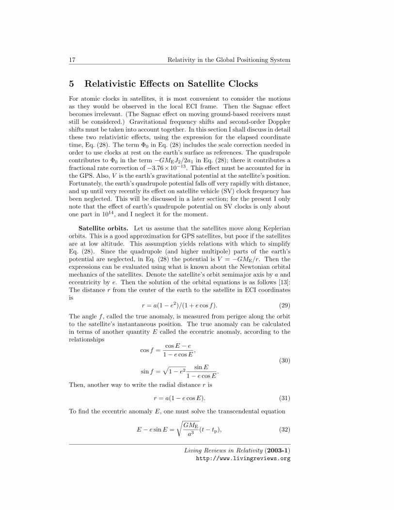
5 Relativistic Effects on Satellite Clocks

For atomic clocks in satellites, it is most convenient to consider the motionsas they would be observed in the local ECI frame. Then the Sagnac effectbecomes irrelevant. (The Sagnac effect on moving ground-based receivers muststill be considered.) Gravitational frequency shifts and second-order Dopplershifts must be taken into account together. In this section I shall discuss in detailthese two relativistic effects, using the expression for the elapsed coordinatetime, Eq. (28). The term Φ0 in Eq. (28) includes the scale correction needed inorder to use clocks at rest on the earth’s surface as references. The quadrupolecontributes to Φ0 in the term −GMEJ2/2a1 in Eq. (28); there it contributes afractional rate correction of −3.76×10−13. This effect must be accounted for inthe GPS. Also, V is the earth’s gravitational potential at the satellite’s position.Fortunately, the earth’s quadrupole potential falls off very rapidly with distance,and up until very recently its effect on satellite vehicle (SV) clock frequency hasbeen neglected. This will be discussed in a later section; for the present I onlynote that the effect of earth’s quadrupole potential on SV clocks is only aboutone part in 1014, and I neglect it for the moment.

Satellite orbits. Let us assume that the satellites move along Keplerianorbits. This is a good approximation for GPS satellites, but poor if the satellitesare at low altitude. This assumption yields relations with which to simplifyEq. (28). Since the quadrupole (and higher multipole) parts of the earth’spotential are neglected, in Eq. (28) the potential is V = −GME/r. Then theexpressions can be evaluated using what is known about the Newtonian orbitalmechanics of the satellites. Denote the satellite’s orbit semimajor axis by a andeccentricity by e. Then the solution of the orbital equations is as follows [13]:The distance r from the center of the earth to the satellite in ECI coordinatesis

r = a(1− e2)/(1 + e cos f). (29)

The angle f , called the true anomaly, is measured from perigee along the orbitto the satellite’s instantaneous position. The true anomaly can be calculatedin terms of another quantity E called the eccentric anomaly, according to therelationships

cos f =cos E − e

1− e cos E,

sin f =√

1− e2sinE

1− e cos E.

(30)

Then, another way to write the radial distance r is

r = a(1− e cos E). (31)

To find the eccentric anomaly E, one must solve the transcendental equation

E − e sinE =

√GME

a3(t− tp), (32)



N. Ashby 18

where tp is the coordinate time of perigee passage.In Newtonian mechanics, the gravitational field is a conservative field and

total energy is conserved. Using the above equations for the Keplerian orbit,one can show that the total energy per unit mass of the satellite is

12v2 − GME

r= −GME

2a. (33)

If I use Eq. (33) for v2 in Eq. (28), then I get the following expression for theelapsed coordinate time on the satellite clock:

∆t =∫

path

dτ

[1 +

3GME

2ac2+

Φ0

c2− 2GME

c2

(1a− 1

r

)]. (34)

The first two constant rate correction terms in Eq. (34) have the values:

3GME

2ac2+

Φ0

c2= +2.5046× 10−10 − 6.9693× 10−10 = −4.4647× 10−10. (35)

The negative sign in this result means that the standard clock in orbit is beatingtoo fast, primarily because its frequency is gravitationally blueshifted. In orderfor the satellite clock to appear to an observer on the geoid to beat at the chosenfrequency of 10.23 MHz, the satellite clocks are adjusted lower in frequency sothat the proper frequency is:[

1− 4.4647× 10−10]× 10.23 MHz = 10.229 999 995 43 MHz. (36)

This adjustment is accomplished on the ground before the clock is placed inorbit.

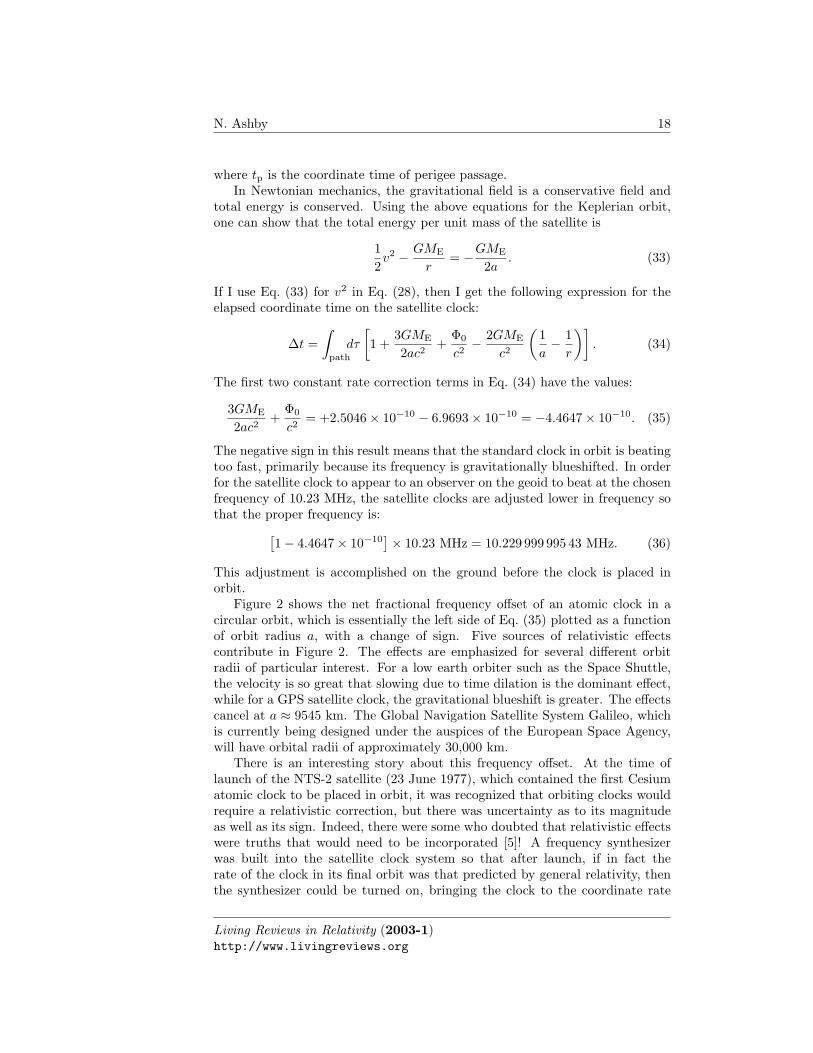
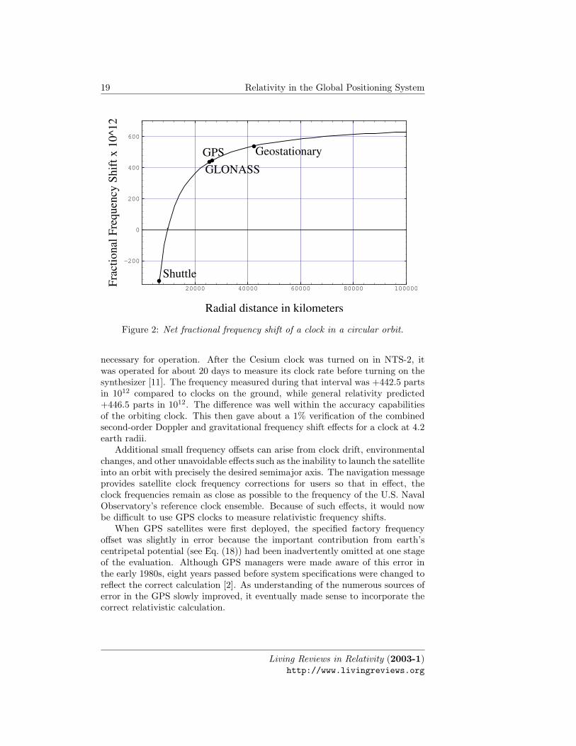
Figure 2 shows the net fractional frequency offset of an atomic clock in acircular orbit, which is essentially the left side of Eq. (35) plotted as a functionof orbit radius a, with a change of sign. Five sources of relativistic effectscontribute in Figure 2. The effects are emphasized for several different orbitradii of particular interest. For a low earth orbiter such as the Space Shuttle,the velocity is so great that slowing due to time dilation is the dominant effect,while for a GPS satellite clock, the gravitational blueshift is greater. The effectscancel at a ≈ 9545 km. The Global Navigation Satellite System Galileo, whichis currently being designed under the auspices of the European Space Agency,will have orbital radii of approximately 30,000 km.

There is an interesting story about this frequency offset. At the time oflaunch of the NTS-2 satellite (23 June 1977), which contained the first Cesiumatomic clock to be placed in orbit, it was recognized that orbiting clocks wouldrequire a relativistic correction, but there was uncertainty as to its magnitudeas well as its sign. Indeed, there were some who doubted that relativistic effectswere truths that would need to be incorporated [5]! A frequency synthesizerwas built into the satellite clock system so that after launch, if in fact therate of the clock in its final orbit was that predicted by general relativity, thenthe synthesizer could be turned on, bringing the clock to the coordinate rate




20000 40000 60000 80000 100000

Radial distance in kilometers

-200

0

200

400

600

Frac

tiona

l Fre

quen

cy S

hift

x 1

0^12

GeostationaryGPSGLONASS

Shuttle

Figure 2: Net fractional frequency shift of a clock in a circular orbit.

necessary for operation. After the Cesium clock was turned on in NTS-2, itwas operated for about 20 days to measure its clock rate before turning on thesynthesizer [11]. The frequency measured during that interval was +442.5 partsin 1012 compared to clocks on the ground, while general relativity predicted+446.5 parts in 1012. The difference was well within the accuracy capabilitiesof the orbiting clock. This then gave about a 1% verification of the combinedsecond-order Doppler and gravitational frequency shift effects for a clock at 4.2earth radii.

Additional small frequency offsets can arise from clock drift, environmentalchanges, and other unavoidable effects such as the inability to launch the satelliteinto an orbit with precisely the desired semimajor axis. The navigation messageprovides satellite clock frequency corrections for users so that in effect, theclock frequencies remain as close as possible to the frequency of the U.S. NavalObservatory’s reference clock ensemble. Because of such effects, it would nowbe difficult to use GPS clocks to measure relativistic frequency shifts.

When GPS satellites were first deployed, the specified factory frequencyoffset was slightly in error because the important contribution from earth’scentripetal potential (see Eq. (18)) had been inadvertently omitted at one stageof the evaluation. Although GPS managers were made aware of this error inthe early 1980s, eight years passed before system specifications were changed toreflect the correct calculation [2]. As understanding of the numerous sources oferror in the GPS slowly improved, it eventually made sense to incorporate thecorrect relativistic calculation.



N. Ashby 20

The eccentricity correction. The last term in Eq. (34) may be integratedexactly by using the following expression for the rate of change of eccentricanomaly with time, which follows by differentiating Eq. (32):

dE

dt=

√GME/a3

1− e cos E. (37)

Also, since a relativistic correction is being computed, ds/c ' dt, so∫ [2GME

c2

(1r− 1

a

)]ds

c' 2GME

c2

∫ (1r− 1

a

)dt

=2GME

ac2

∫dt

(e cos E

1− e cos E

)=

2√

GMEa

c2e (sinE − sinE0)

= +2√

GMEa

c2e sinE + constant. (38)

The constant of integration in Eq. (38) can be dropped since this term is lumpedwith other clock offset effects in the Kalman filter computation of the clockcorrection model. The net correction for clock offset due to relativistic effectsthat vary in time is

∆tr = +4.4428× 10−10e√

a sinEs√m

. (39)

This correction must be made by the receiver; it is a correction to the coordinatetime as transmitted by the satellite. For a satellite of eccentricity e = 0.01, themaximum size of this term is about 23 ns. The correction is needed becauseof a combination of effects on the satellite clock due to gravitational frequencyshift and second-order Doppler shift, which vary due to orbit eccentricity.

Eq. (39) can be expressed without approximation in the alternative form

∆tr = +2r · v

c2, (40)

where r and v are the position and velocity of the satellite at the instant oftransmission. This may be proved using the expressions (30, 31, 32) for theKeplerian orbits of the satellites. This latter form is usually used in implemen-tations of the receiver software.

It is not at all necessary, in a navigation satellite system, that the eccen-tricity correction be applied by the receiver. It appears that the clocks in theGLONASS satellite system do have this correction applied before broadcast. Infact historically, this was dictated in the GPS by the small amount of computingpower available in the early GPS satellite vehicles. It would actually make moresense to incorporate this correction into the time broadcast by the satellites;then the broadcast time events would be much closer to coordinate time – thatis, GPS system time. It may now be too late to reverse this decision because of




the investment that many dozens of receiver manufacturers have in their prod-ucts. However, it does mean that receivers are supposed to incorporate therelativity correction; therefore, if appropriate data can be obtained in raw formfrom a receiver one can measure this effect. Such measurements are discussednext.



N. Ashby 22

6 TOPEX/POSEIDON Relativity Experiment

Recently, a report distributed by the Aerospace Corporation [14] claimed thatthe correction expressed in Eqs. (38) and (39) would not be valid for a highlydynamic receiver – e.g., one in a highly eccentric orbit. This is a conceptualerror, emanating from an apparently official source, which would have seriousconsequences. The GPS modernization program involves significant redesignand remanufacturing of the Block IIF satellites, as well as a new generationof satellites that is now on the drawing boards – the Block IIR replenishmentsatellites. These satellites are capable of autonomous operation, that is, theycan be operated independently of the ground-based control segment for up to180 days. They are to accomplish this by having receivers on board that deter-mine their own position and time by listening to the other satellites that are inview. If the conceptual basis for accounting for relativity in the GPS, as it hasbeen explained above, were invalid, the costs of opening up these satellites andreprogramming them would be astronomical.

There has been therefore considerable controversy about this issue. As aconsequence, it was proposed by William Feess of the Aerospace Corporationthat a measurement of this effect be made using the receiver on board theTOPEX satellite. The TOPEX satellite carries an advanced, six-channel GPSreceiver. With six data channels available, five of the channels can be used todetermine the bias on the local oscillator of the TOPEX receiver with someredundancy, and data from the sixth channel can be used to measure the ec-centricity effect on the sixth SV clock. Here I present some preliminary resultsof these measurements, which are to my knowledge the first explicit measure-ments of the periodic part of the combined relativistic effects of time dilationand gravitational frequency shift on an orbiting receiver.

A brief description of the pseudorange measurement made by a receiveris needed here before explaining the TOPEX data. Many receivers work bygenerating a replica of the coded signal emanating from the transmitter. Thisreplica, which is driven through a feedback shift register at a rate matching theDoppler-shifted incoming signal, is correlated with the incoming signal. Thetransmitted coordinate time can be identified in terms of a particular phasereversal at a particular point within the code train of the signal. When thecorrelator in the receiver is locked onto the incoming signal, the time delaybetween the transmission event and the arrival time, as measured on the localclock, can be measured at any chosen instant.

Let the time as transmitted from the jth satellite be denoted by t′j . Aftercorrecting for the eccentricity effect, the GPS time of transmission would bet′j + (∆tr)j . Because of SA (which was in effect for the data that were chosen),frequency offsets and frequency drifts, the satellite clock may have an additionalerror bj so that the true GPS transmission time is tj = t′j + (∆tr)j − bj .

Now the local clock, which is usually a free-running oscillator subject to var-ious noise and drift processes, can be in error by a large amount. Let the mea-sured reception time be t′R and the true GPS time of reception be tR = t′R− bR.The possible existence of this local clock bias is the reason why measurements




from four satellites are needed for navigation, as from four measurements thethree components of the receiver’s position vector, and the local clock bias, canbe determined. The raw difference between the time of reception of the time tagfrom the satellite, and the time of transmission, multiplied by c, is an estimateof the geometric range between satellite and receiver called the pseudorange [22]:

ρj = c(t′R − t′j) = c [(tR + bR)− (tj + bj − (∆tr)j)] . (41)

On the other hand the true range between satellite and receiver is

|rR(tR)− rj(tj)| = c(tR − tj). (42)

Combining Eqs. (41)and (42) yields the measurement equation for this experi-ment:

|rR(tR)− rj(tj)| − ρj + cbR − cbj + c(∆tr)j = 0. (43)

The purpose of the TOPEX satellite is to measure the height of the sea. Thissatellite has a six-channel receiver on board with a very good quartz oscillatorto provide the time reference. A radar altimeter measures the distance of thesatellite from the surface of the sea, but such measurements play no role in thepresent experiment. The TOPEX satellite has orbit radius 7,714 km, an orbitalperiod of about 6745 seconds, and an orbital inclination of 66.06 to earth’sequatorial plane. Except for perturbations due to earth’s quadrupole moment,the orbit is very nearly circular, with eccentricity being only 0.000057. TheTOPEX satellite is almost ideal for analysis of this relativity effect. The trajec-tories of the TOPEX and GPS satellites were determined independently of theon-board clocks, by means of Doppler tracking from ≈ 100 stations maintainedby the Jet Propulsion Laboratory (JPL).

The receiver is a dual frequency C/A- and P-code receiver from which bothcode data and carrier phase data were obtained. The dual-frequency measure-ments enabled us to correct the propagation delay times for electron contentin the ionosphere. Close cooperation was given by JPL and by William Feessin providing the dual-frequency measurements, which are ordinarily denied tocivilian users, and in removing the effect of SA at time points separated by 300seconds during the course of the experiment.

The following data were provided through the courtesy of Yoaz Bar-Sever ofJPL for October 22–23, 1995:

• ECI center-of-mass position and velocity vectors for 25 satellites, in theJ2000 Coordinate system with times in UTC. Data rate is every 15 min-utes; accuracy quoted is 10 cm radial, 30 cm horizontal.

• ECI position and velocity vectors for the TOPEX antenna phase center.Data rate is every minute in UTC; accuracy quoted is 3 cm radial and10 cm horizontal.

• GPS satellite clock data for 25 satellites based on ground system observa-tions. Data rate is every 5 minutes, in GPS time; accuracy ranges between5 and 10 cm.



N. Ashby 24

• TOPEX dual frequency GPS receiver measurements of pseudorange andcarrier phase for 25 satellites, a maximum of six at any one time. Thedata rate is every 10 seconds, in GPS time.

During this part of 1995, GPS time was ahead of UTC by 10 seconds. GPScannot tolerate leap seconds so whenever a leap second is inserted in UTC,UTC falls farther behind GPS time. This required high-order interpolationon the orbit files to obtain positions and velocities at times corresponding totimes given, every 300 seconds, in the GPS clock data files. When this wasdone independently by William Feess and myself we agreed typically to withina millimeter in satellite positions.

The L1 and L2 carrier phase data was first corrected for ionospheric delay.Then the corrected carrier phase data was used to smooth the pseudorange databy weighted averaging. SA was compensated in the clock data by courtesy ofWilliam Feess. Basically, the effect of SA is contained in both the clock dataand in the pseudorange data and can be eliminated by appropriate subtraction.Corrections for the offset of the GPS SV antenna phase centers from the SVcenters of mass were also incorporated.

The determination of the TOPEX clock bias is obtained by rearrangingEq. (43):

|rR(tR)− rj(tj)| − ρj − cbj + c∆tr = −cbR. (44)

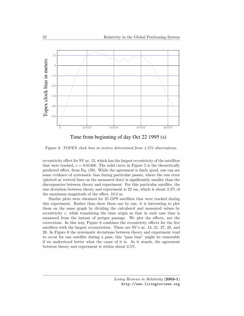
Generally, at each time point during the experiment, observations were obtainedfrom six (sometimes five) satellites. The geometric range, the first term inEq. (44), was determined by JPL from independent Doppler tracking of boththe GPS constellation and the TOPEX satellite. The pseudorange was directlymeasured by the receiver, and clock models provided the determination of theclock biases cbj in the satellites. The relativity correction for each satellite canbe calculated directly from the given GPS satellite orbits. Because the receiveris a six-channel receiver, there is sufficient redundancy in the measurements toobtain good estimates of the TOPEX clock bias and the rms error in this biasdue to measurement noise. The resulting clock bias is plotted in Figure 3.

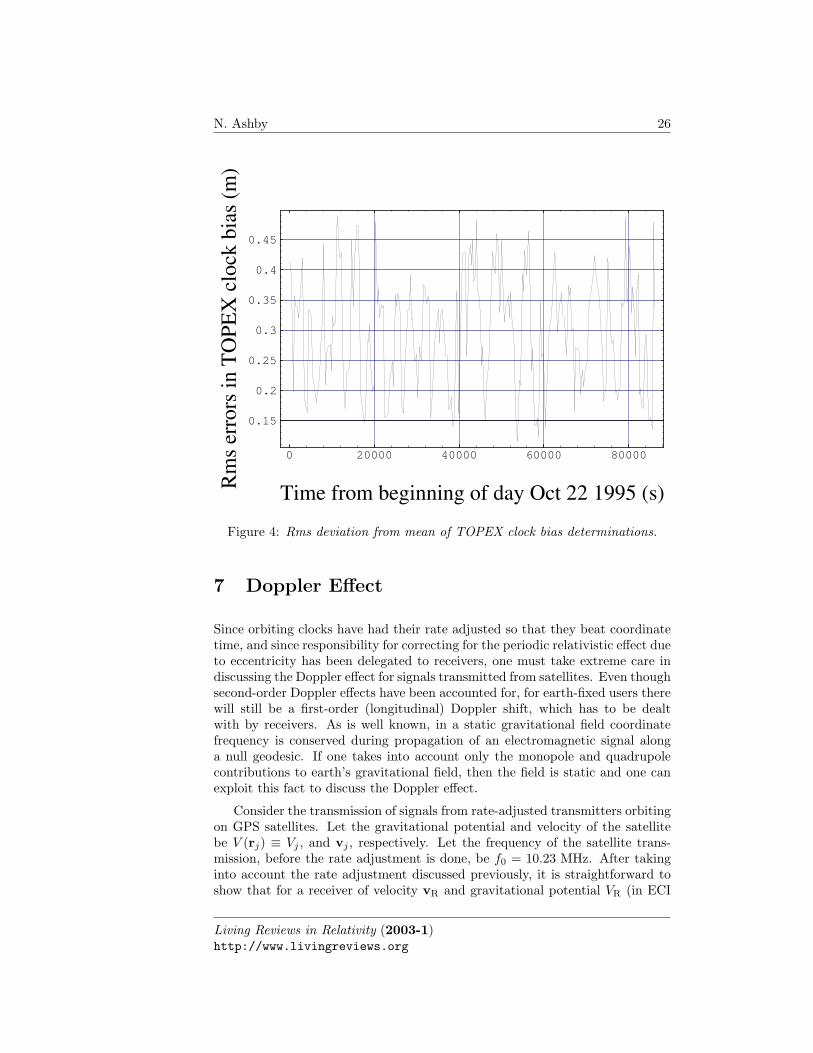
The rms deviation from the mean of the TOPEX clock biases is plotted inFigure 4 as a function of time. The average rms error is 29 cm, correspondingto about one ns of propagation delay. Much of this variation can be attributedto multipath effects.

Figure 3 shows an overall frequency drift, accompanied by frequency adjust-ments and a large periodic variation with period equal to the orbital period.Figure 3 gives our best estimate of the TOPEX clock bias. This may now beused to measure the eccentricity effects by rearranging Eq. (43):

|rR(tR)− rj(tj)| − ρj − cbj + cbR = −c∆tr. (45)

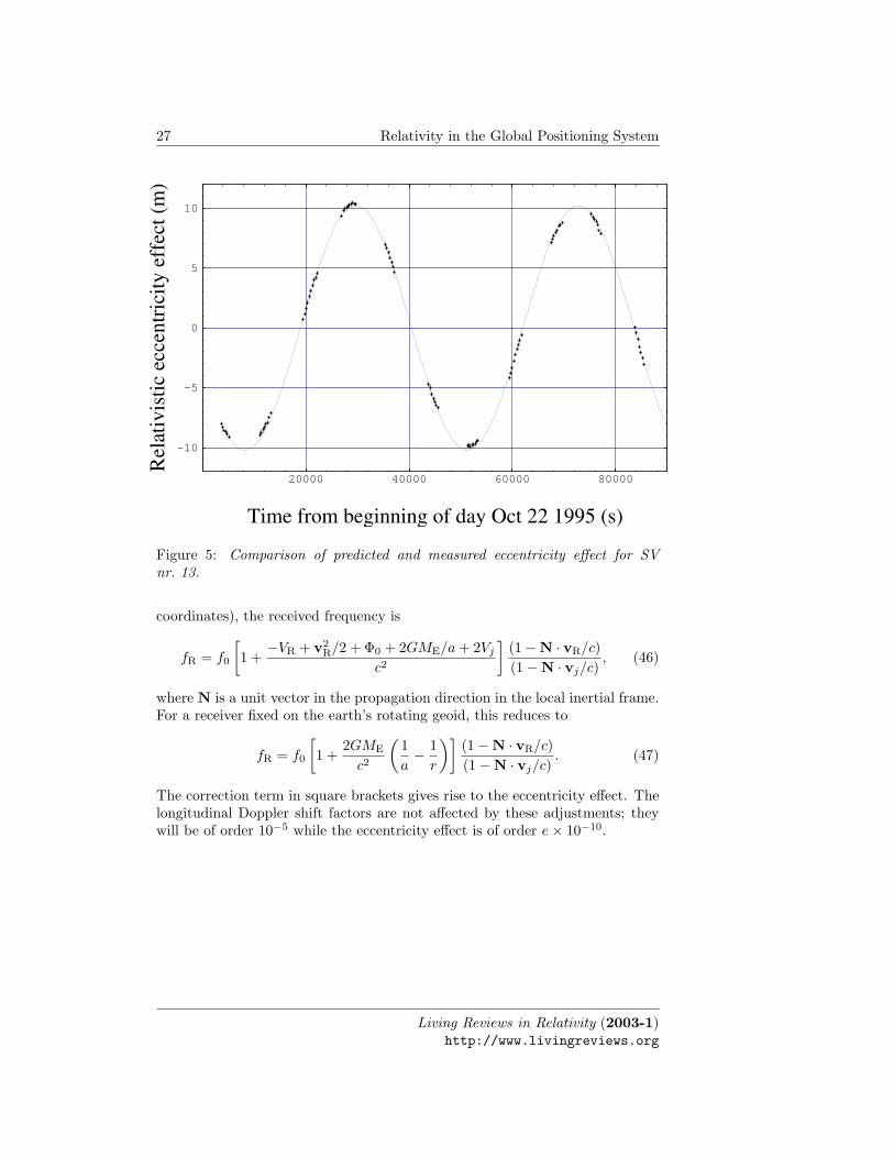
Strictly speaking, in finding the eccentricity effect this way for a particularsatellite, one should not include data from that satellite in the determinationof the clock bias. One can show, however, that the penalty for this is simply toincrease the rms error by a factor of 6/5, to 35 cm. Figure 5 shows the measured




0 20000 40000 60000 80000

Time from beginning of day Oct 22 1995 (s)

-50

-40

-30

-20

-10

0

10

Top

ex c

lock

bia

s in

met

ers

Figure 3: TOPEX clock bias in meters determined from 1,571 observations.

eccentricity effect for SV nr. 13, which has the largest eccentricity of the satellitesthat were tracked, e = 0.01486. The solid curve in Figure 5 is the theoreticallypredicted effect, from Eq. (39). While the agreement is fairly good, one can seesome evidence of systematic bias during particular passes, where the rms error(plotted as vertical lines on the measured dots) is significantly smaller than thediscrepancies between theory and experiment. For this particular satellite, therms deviation between theory and experiment is 22 cm, which is about 2.2% ofthe maximum magnitude of the effect, 10.2 m.

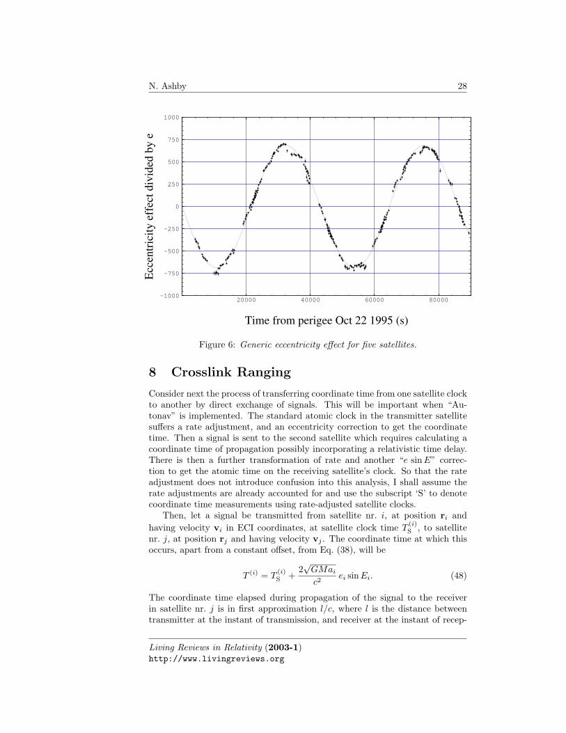
Similar plots were obtained for 25 GPS satellites that were tracked duringthis experiment. Rather than show them one by one, it is interesting to plotthem on the same graph by dividing the calculated and measured values byeccentricity e, while translating the time origin so that in each case time ismeasured from the instant of perigee passage. We plot the effects, not thecorrections. In this way, Figure 6 combines the eccentricity effects for the fivesatellites with the largest eccentricities. These are SV’s nr. 13, 21, 27, 23, and26. In Figure 6 the systematic deviations between theory and experiment tendto occur for one satellite during a pass; this “pass bias” might be removableif we understood better what the cause of it is. As it stands, the agreementbetween theory and experiment is within about 2.5%.



N. Ashby 26

0 20000 40000 60000 80000


0.15

0.2

0.25

0.3

0.35

0.4

0.45R

ms

erro

rs in

TO

PEX

clo

ck b

ias

(m)

Figure 4: Rms deviation from mean of TOPEX clock bias determinations.

7 Doppler Effect

Since orbiting clocks have had their rate adjusted so that they beat coordinatetime, and since responsibility for correcting for the periodic relativistic effect dueto eccentricity has been delegated to receivers, one must take extreme care indiscussing the Doppler effect for signals transmitted from satellites. Even thoughsecond-order Doppler effects have been accounted for, for earth-fixed users therewill still be a first-order (longitudinal) Doppler shift, which has to be dealtwith by receivers. As is well known, in a static gravitational field coordinatefrequency is conserved during propagation of an electromagnetic signal alonga null geodesic. If one takes into account only the monopole and quadrupolecontributions to earth’s gravitational field, then the field is static and one canexploit this fact to discuss the Doppler effect.

Consider the transmission of signals from rate-adjusted transmitters orbitingon GPS satellites. Let the gravitational potential and velocity of the satellitebe V (rj) ≡ Vj , and vj , respectively. Let the frequency of the satellite trans-mission, before the rate adjustment is done, be f0 = 10.23 MHz. After takinginto account the rate adjustment discussed previously, it is straightforward toshow that for a receiver of velocity vR and gravitational potential VR (in ECI




20000 40000 60000 80000


-10

-5

0

5

10

Rel

ativ

istic

ecc

entr

icity

eff

ect (

m)

Figure 5: Comparison of predicted and measured eccentricity effect for SVnr. 13.

coordinates), the received frequency is

fR = f0

[1 +

−VR + v2R/2 + Φ0 + 2GME/a + 2Vj

c2

](1−N · vR/c)(1−N · vj/c)

, (46)

where N is a unit vector in the propagation direction in the local inertial frame.For a receiver fixed on the earth’s rotating geoid, this reduces to

fR = f0

[1 +

2GME

c2

(1a− 1

r

)](1−N · vR/c)(1−N · vj/c)

. (47)

The correction term in square brackets gives rise to the eccentricity effect. Thelongitudinal Doppler shift factors are not affected by these adjustments; theywill be of order 10−5 while the eccentricity effect is of order e× 10−10.



N. Ashby 28

20000 40000 60000 80000

Time from perigee Oct 22 1995 (s)

-1000

-750

-500

-250

0

250

500

750

1000

Ecc

entr

icity

eff

ect d

ivid

ed b

y e

Figure 6: Generic eccentricity effect for five satellites.

8 Crosslink Ranging

Consider next the process of transferring coordinate time from one satellite clockto another by direct exchange of signals. This will be important when “Au-tonav” is implemented. The standard atomic clock in the transmitter satellitesuffers a rate adjustment, and an eccentricity correction to get the coordinatetime. Then a signal is sent to the second satellite which requires calculating acoordinate time of propagation possibly incorporating a relativistic time delay.There is then a further transformation of rate and another “e sinE” correc-tion to get the atomic time on the receiving satellite’s clock. So that the rateadjustment does not introduce confusion into this analysis, I shall assume therate adjustments are already accounted for and use the subscript ‘S’ to denotecoordinate time measurements using rate-adjusted satellite clocks.

Then, let a signal be transmitted from satellite nr. i, at position ri andhaving velocity vi in ECI coordinates, at satellite clock time T

(i)S , to satellite

nr. j, at position rj and having velocity vj . The coordinate time at which thisoccurs, apart from a constant offset, from Eq. (38), will be

T (i) = T(i)S +

2√

GMai

c2ei sinEi. (48)

The coordinate time elapsed during propagation of the signal to the receiverin satellite nr. j is in first approximation l/c, where l is the distance betweentransmitter at the instant of transmission, and receiver at the instant of recep-




tion: ∆T = T (j) − T (i) = l/c. The Shapiro time delay corrections to this willbe discussed in the next section. Finally, the coordinate time of arrival of thesignal is related to the time on the receiving satellite’s adjusted clock by theinverse of Eq. (48):

T(j)S = T (j) −

2√

GMaj

c2ej sinEj . (49)

Collecting these results, we get

T(j)S = T

(i)S +

l

c−

2√

GMaj

c2ej sinEj +

2√

GMai

c2ei sinEi. (50)

In Eq. (50) the distance l is the actual propagation distance, in ECI coordinates,of the signal. If this is expressed instead in terms of the distance |∆r| = |rj(ti)−ri(ti)| between the two satellites at the instant of transmission, then

l = |∆r|+ ∆r · vj

c. (51)

The extra term accounts for motion of the receiver through the inertial frameduring signal propagation. Then Eq. (50) becomes

T(j)S = T

(i)S +

|∆r|c

− 2√

GMa2

c2ej sinEj +

2√

GMai

c2ei sinEi +

∆r · vj

c2. (52)

This result contains all the relativistic corrections that need to be consideredfor direct time transfer by transmission of a time-tagged pulse from one satelliteto another. The last term in Eq. (52) should not be confused with the correctionof Eq. (40).



N. Ashby 30

9 Frequency Shifts Induced by Orbit Changes

Improvements in GPS motivate attention to other small relativistic effects thathave previously been too small to be explicitly considered. For SV clocks, theseinclude frequency changes due to orbit adjustments, and effects due to earth’soblateness. For example, between July 25 and October 10, 2000, SV43 occupieda transfer orbit while it was moved from slot 5 to slot 3 in orbit plane F. I willshow here that the fractional frequency change associated with a change da inthe semi-major axis a (in meters) can be estimated as 9.429× 10−18da. In thecase of SV43, this yields a prediction of −1.77 × 10−13 for the fractional fre-quency change of the SV43 clock which occurred 25 July 2000. This relativisticeffect was recently measured very carefully [12]. Another orbit adjustment onOctober 10, 2000 should have resulted in another fractional frequency changeof +1.75 × 10−13, which has not yet been measured carefully. Also, earth’soblateness causes a periodic fractional frequency shift with period of almost 6hours and amplitude 0.695× 10−14. This means that quadrupole effects on SVclock frequencies are of the same general order of magnitude as the frequencybreaks induced by orbit changes. Thus, some approximate expressions for thefrequency effects on SV clock frequencies due to earth’s oblateness are needed.These effects will be discussed with the help of Lagrange’s planetary perturba-tion equations.

Five distinct relativistic effects, discussed in Section 5, are incorporated intothe System Specification Document, ICD-GPS-200 [2]. These are:

• the effect of earth’s mass on gravitational frequency shifts of atomic ref-erence clocks fixed on the earth’s surface relative to clocks at infinity;

• the effect of earth’s oblate mass distribution on gravitational frequencyshifts of atomic clocks fixed on earth’s surface;

• second-order Doppler shifts of clocks fixed on earth’s surface due to earthrotation;

• gravitational frequency shifts of clocks in GPS satellites due to earth’smass;

• and second-order Doppler shifts of clocks in GPS satellites due to theirmotion through an Earth-Centered Inertial (ECI) Frame.

The combination of second-order Doppler and gravitational frequency shiftsgiven in Eq. (27) for a clock in a GPS satellite leads directly to the followingexpression for the fractional frequency shift of a satellite clock relative to areference clock fixed on earth’s geoid:

∆f

f= −1

2v2

c2− GME

rc2− Φ0

c2, (53)

where v is the satellite speed in a local ECI reference frame, GME is the productof the Newtonian gravitational constant G and earth’s mass M , c is the defined




speed of light, and Φ0 is the effective gravitational potential on the earth’srotating geoid. The term Φ0 includes contributions from both monopole andquadrupole moments of earth’s mass distribution, and the effective centripetalpotential in an earth-fixed reference frame such as the WGS-84(837) frame,due to earth’s rotation. The value for Φ0 is given in Eq. (18), and dependson earth’s equatorial radius a1, earth’s quadrupole moment coefficient J2, andearth’s angular rotational speed ωE.

If the GPS satellite orbit can be approximated by a Keplerian orbit of semi-major axis a, then at an instant when the distance of the clock from earth’scenter of mass is r, this leads to the following expression for the fraction fre-quency shift of Eq. (53):

∆f

f= −3GME

2ac2− Φ0

c2+

2GME

c2

[1r− 1

a

]. (54)

Eq. (54) is derived by making use of the conservation of total energy (per unitmass) of the satellite, Eq. (33), which leads to an expression for v2 in termsof GME/r and GME/a that can be substituted into Eq. (53). The first twoterms in Eq. (54) give rise to the “factory frequency offset”, which is applied toGPS clocks before launch in order to make them beat at a rate equal to that ofreference clocks on earth’s surface. The last term in Eq. (54) is very small whenthe orbit eccentricity e is small; when integrated over time these terms give riseto the so-called “e sinE” effect or “eccentricity effect”. In most of the followingdiscussion we shall assume that eccentricity is very small.

Clearly, from Eq. (54), if the semi-major axis should change by an amountδa due to an orbit adjustment, the satellite clock will experience a fractionalfrequency change

δf

f= +

3GMEδa

2c2a2. (55)

The factor 3/2 in this expression arises from the combined effect of second-orderDoppler and gravitational frequency shifts. If the semi-major axis increases, thesatellite will be higher in earth’s gravitational potential and will be gravitation-ally blue-shifted more, while at the same time the satellite velocity will bereduced, reducing the size of the second-order Doppler shift (which is generallya red shift). The net effect would make a positive contribution to the fractionalfrequency shift.

Although it has long been known that orbit adjustments are associated withsatellite clock frequency shifts, nothing has been documented and up until re-cently no reliable measurements of such shifts have been made. On July 25,2000, a trajectory change was applied to SV43 to shift the satellite from slot F5to slot F3. A drift orbit extending from July 25, 2000 to October 10, 2000 wasused to accomplish this move. A “frequency break” was observed but the causeof this frequency jump was not initially understood. Recently, Marvin Epstein,Joseph Fine, and Eric Stoll [12] of ITT have evaluated the frequency shift ofSV43 arising from this trajectory change. They reported that associated withthe thruster firings on July 25, 2000 there was a frequency shift of the Rubidium



N. Ashby 32

clock on board SV43 of amount

δf

f= −1.85× 10−13 (measured). (56)

Epstein et al. [12] suggested that the above frequency shift was relativisticin origin, and used precise ephemerides obtained from the National Imageryand Mapping Agency to estimate the frequency shift arising from second-orderDoppler and gravitational potential differences. They calculated separately thesecond-order Doppler and gravitational frequency shifts due to the orbit change.The NIMA precise ephemerides are expressed in the WGS-84 coordinate frame,which is earth-fixed. If used without removing the underlying earth rotation,the velocity would be erroneous. They therefore transformed the NIMA preciseephemerides to an earth-centered inertial frame by accounting for a (uniform)earth rotation rate.

The semi-major axes before and after the orbit change were calculated bytaking the average of the maximum and minimum radial distances. Speedswere calculated using a Keplerian orbit model. They arrived at the followingnumerical values for semi-major axis and velocity:

07/22/00 : a = 2.656139556× 107 m; v = 3.873947951× 103 m s−1,

07/30/00 : a = 2.654267359× 107 m; v = 3.875239113× 103 m s−1.

Since the semi-major axis decreased, the frequency shift should be negative.The prediction they made for the frequency shift, which was based on Eq. (53),was then

δf

f= −1.734× 10−13, (57)

which is to be compared with the measured value, Eq. (56). This is fairlycompelling evidence that the observed frequency shift is indeed a relativisticeffect.

Lagrange perturbation theory. Perturbations of GPS orbits due toearth’s quadrupole mass distribution are a significant fraction of the change insemi-major axis associated with the orbit change discussed above. This raisesthe question whether it is sufficiently accurate to use a Keplerian orbit to de-scribe GPS satellite orbits, and estimate the semi-major axis change as thoughthe orbit were Keplerian. In this section, we estimate the effect of earth’squadrupole moment on the orbital elements of a nominally circular orbit andthence on the change in frequency induced by an orbit change. Previously, suchan effect on the SV clocks has been neglected, and indeed it does turn out to besmall. However, the effect may be worth considering as GPS clock performancecontinues to improve.

To see how large such quadrupole effects may be, we use exact calcula-tions for the perturbations of the Keplerian orbital elements available in theliterature [13]. For the semi-major axis, if the eccentricity is very small, the




dominant contribution has a period twice the orbital period and has ampli-tude 3J2a

21 sin2 i0/(2a0) ≈ 1658 m. WGS-84(837) values for the following ad-

ditional constants are used in this section: a1 = 6.3781370 × 106 m; ωE =7.291151467 × 10−5 s−1; a0 = 2.656175 × 107 m, where a1 and a0 are earth’sequatorial radius and SV orbit semi-major axis, and ωE is earth’s rotationalangular velocity.

The oscillation in the semi-major axis would significantly affect calculationsof the semi-major axis at any particular time. This suggests that Eq. (33) needsto be reexamined in light of the periodic perturbations on the semi-major axis.Therefore, in this section we develop an approximate description of a satelliteorbit of small eccentricity, taking into account earth’s quadrupole moment tofirst order. Terms of order J2 × e will be neglected. This problem is non-trivial because the perturbations themselves (see, for example, the equations formean anomaly and altitude of perigee) have factors 1/e which blow up as theeccentricity approaches zero. This problem is a mathematical one, not a physicalone. It simply means that the observable quantities – such as coordinates andvelocities – need to be calculated in such a way that finite values are obtained.Orbital elements that blow up are unobservable.

Conservation of energy. The gravitational potential of a satellite atposition (x, y, z) in equatorial ECI coordinates in the model under considerationhere is

V (x, y, z) = −GME

r

(1− J2a

21

r2

[3z2

2r2− 1

2

]). (58)

Since the force is conservative in this model (solar radiation pressure, thrust,etc. are not considered), the kinetic plus potential energy is conserved. Let εbe the energy per unit mass of an orbiting mass point. Then

ε = constant =v2

2+ V (x, y, z) =

v2

2− GME

r+ V ′(x, y, z), (59)

where V ′(x, y, z) is the perturbing potential due to the earth’s quadrupole po-tential. It is shown in textbooks [13] that, with the help of Lagrange’s planetaryperturbation theory, the conservation of energy condition can be put in the form

ε = −GME

2a+ V ′(x, y, z), (60)

where a is the perturbed (osculating) semi-major axis. In other words, for theperturbed orbit,

v2

2− GME

r= −GME

2a. (61)

On the other hand, the net fractional frequency shift relative to a clock at restat infinity is determined by the second-order Doppler shift (a red shift) and agravitational redshift. The total relativistic fractional frequency shift is

∆f

f= −v2

2− GME

r+ V ′(x, y, z). (62)



N. Ashby 34

The conservation of energy condition can be used to express the second-orderDoppler shift in terms of the potential. Since in this paper we are interestedin fractional frequency changes caused by changing the orbit, it will make nodifference if the calculations use a clock at rest at infinity as a reference ratherthan a clock at rest on earth’s surface. The reference potential cancels out tothe required order of accuracy. Therefore, from perturbation theory we needexpressions for the square of the velocity, for the radius r, and for the perturb-ing potential. We now proceed to derive these expressions. We refer to theliterature [13] for the perturbed osculating elements. These are exactly known,to all orders in the eccentricity, and to first order in J2. We shall need only theleading terms in eccentricity e for each element.

Perturbation equations. First we recall some facts about an unperturbedKeplerian orbit, which have already been introduced (see Section 5). The ec-centric anomaly E is to be calculated by solving the equation

E − e sinE = M = n0(t− t0), (63)

where M is the “mean anomaly” and t0 is the time of passage past perigee, and

n0 =√

GME/a3. (64)

Then, the perturbed radial distance r and true anomaly f of the satellite areobtained from

r = a(1− e cos E), (65)

cos f =cos E − e

1− e cos E, sin f =

√1− e2

sinE

1− e cos E. (66)

The observable x, y, z-coordinates of the satellite are then calculated from thefollowing equations:

x = r(cos Ω cos(f + ω)− cos i sinΩ sin(f + ω)), (67)y = r(sinΩ cos(f + ω) + cos i cos Ω sin(f + ω)), (68)z = r(sin i sin(f + ω)), (69)

where Ω is the angle of the ascending line of nodes, i is the inclination, and ωis the altitude of perigee. By differentiation with respect to time, or by usingthe conservation of energy equation, one obtains the following expression for thesquare of the velocity:

v2 =GME

a

1 + e cos E

1− e cos E. (70)

In these expressions v2 and r−1 are observable quantities. The combinatione cos E, where E is the eccentric anomaly, occurs in both of these expressions.To derive expressions for v2 and r−1 in the perturbed orbits, expressions for theperturbed elements a, e, E are to be substituted into the right-hand sides ofthe Keplerian equations for E, r, and v2. Therefore, we need the combinatione cos E in the limit of small eccentricity.




Perturbed eccentricity. To leading order, from the literature [13] we havefor the perturbed eccentricity the following expression:

e = e0 +3J2a

21

2a20

[(1− 3

2sin2 i0

)cos f +

14

sin2 i0 cos(2ω0 + f)

+712

sin2 i0 cos(2ω0 + 3f)], (71)

where e0 is a constant of integration.

Perturbed eccentric anomaly. The eccentric anomaly is calculated fromthe equation

E = M + e sinE, (72)

with perturbed values for M and e. Expanding to first order in e gives thefollowing expression for cos E:

cos E = cos M − e sinM sinE, (73)

and multiplying by e yields

e cos E = e cos M − e2 sinM sinE ≈ e cos M. (74)

We shall neglect higher order terms in e. The perturbed expression for meananomaly M can be written as

M = M0 + ∆M/e0, (75)

where we indicate explicitly the terms in e−10 ; that is, the quantity M0 contains

all terms which do not blow up as e → 0, and ∆M/e0 contains all the otherterms. The perturbations of M are known exactly but we shall only need theleading order terms, which are

∆M/e0 = −3J2a21

2e0a20

[(1− 3

2sin2 i0

)sin f − 1

4sin2 i0 sin(2ω0 + f)

+712

sin2 i0 sin(2ω0 + 3f)], (76)

and so for very small eccentricity,

e cos E = e cos M0 −∆M sinM0. (77)

Then after accounting for contributions from the perturbed eccentricity and theperturbed mean anomaly, after a few lines of algebra we obtain the followingfor e cos E:

e cos E = e0 cos E0 +3J2a

21

2a20

(1− 3

2sin2 i0

)+

5J2a21

4a20

sin2 i0 cos 2(ω0 + f), (78)



N. Ashby 36

where the first term is the unperturbed part. The perturbation is a constant,plus a term with twice the orbital period.

Perturbation in semi-major axis. From the literature, the leading termsin the perturbation of the semi-major axis are

a = a0 +3J2a

21

2a0sin2 i0 cos 2(ω0 + f), (79)

where a0 is a constant of integration. The amplitude of the periodic term isabout 1658 meters.

Perturbation in radius. We are now in position to compute the per-turbation in the radius. From the expression for r, after combining terms wehave

r = a0(1− e0 cos E0) + ∆a−∆(e cos E)

= a0(1− e0 cos E0)−3J2a

21

2a0

(1− 3

2sin2 i0

)+

J2a21

4a0sin2 i0 cos 2(ω0 + f). (80)

The amplitude of the periodic part of the perturbation in the observable radialdistance is only 276 meters.

Perturbation in the velocity squared. The above results, after substi-tuting into Eq. (70), yield the expression

v2

2=

GME

2a0(1 + 2e0 cos E0) +

3GMEJ2a21

a30

(1− 3

2sin2 i0

)+

GMEJ2a21

2a30

sin2 i0 cos 2(ω0 + f). (81)

Perturbation in GME/r. The above expression for the perturbed r yieldsthe following for the monopole contribution to the gravitational potential:

− GME

r= −GME

a0(1 + e0 cos E0)−

3GMEJ2a21

2a30

(1− 3

2sin2 i0

)+

GMEJ2a21 sin2 i0

4a30

cos 2(ω0 + f). (82)

Evaluation of the perturbing potential. Since the perturbing potentialcontains the small factor J2, to leading order we may substitute unperturbedvalues for r and z into V ′(x, y, z), which yields the expression

V ′(x, y, z) = −GMEJ2a21

2a30

(1− 3

2sin2 i0

)− 3GMEJ2a

21 sin2 i0

4a30

cos 2(ω0 + f).

(83)




Conservation of energy. It is now very easy to check conservation of en-ergy. Adding kinetic energy per unit mass to two contributions to the potentialenergy gives

ε =v2

2− GME

r+ V ′ = −GME

2a0− GMEJ2a

21

2a30

(1− 3

2sin2 i0

). (84)

This verifies that the perturbation theory gives a constant energy. The extraterm in the above equation, with J2 in it, can be neglected. This is becausethe nominal inclination of GPS orbits is such that the factor (1 − 3 sin2 i0/2)is essentially zero. The near vanishing of this factor is pure coincidence in theGPS. There was no intent, in the original GPS design, that quadrupole effectswould be simpler if the orbital inclination were close to 55. However, becausethis term is negligible, numerical calculations of the total energy per unit massprovide a means of evaluating the quantity a0.

Calculation of fractional frequency shift. The fractional frequencyshift calculation is very similar to the calculation of the energy, except that thesecond-order Doppler term contributes with a negative sign. The result is

∆f

f= − v2

2c2− GME

c2r+

V ′

c2

= −3GME

2a0c2− 2GME

c2a0e0 cos E0 −

7GMEJ2a21

2a30c

2

(1− 3

2sin2 i0

)−GMEJ2a

21 sin2 i0

a30c

2cos 2(ω0 + f). (85)

The first term, when combined with the reference potential at earth’s geoid,gives rise to the “factory frequency offset”. The seond term gives rise to theeccentricity effect. The third term can be neglected, as pointed out above. Thelast term has an amplitude

GMEJ2a21 sin2 i0

a30c

2= 6.95× 10−15, (86)

which may be large enough to consider when calculating frequency shifts pro-duced by orbit changes. Therefore, this contribution may have to be consideredin the future in the determination of the semi-major axis, but for now we neglectit.

The result suggests the following method of computing the fractional fre-quency shift: Averaging the shift over one orbit, the periodic term will averagedown to a negligible value. The third term is negligible. So if one has a good esti-mate for the nominal semi-major axis parameter, the term −3GME/2a0c

2 givesthe average fractional frequency shift. On the other hand, the average energyper unit mass is given by ε = −GME/2a0. Therefore, the precise ephemerides,specified in an ECI frame, can be used to compute the average value for ε; then



N. Ashby 38

the average fractional frequency shift will be

∆f

f= 3ε/c2. (87)

The last periodic term in Eq. (85) is of a form similar to that which gives riseto the eccentricity correction, which is applied by GPS receivers. Consideringonly the last periodic term, the additional time elapsed on the orbiting clockwill be given by

δtJ2 =∫

path

dt

[−GMEJ2a

21 sin2 i0

a30c

2cos(2ω0 + 2nt)

], (88)

where to a sufficient approximation we have replaced the quantity f in theintegrand by n =

√GME/a3

0; n is the approximate mean motion of GPS satel-lites. Integrating and dropping the constant of integration (assuming as usualthat such constant time offsets are lumped with other contributions) gives theperiodic relativistic effect on the elapsed time of the SV clock due to earth’squadrupole moment:

δtJ2 = −

√GME

a30

J2a21 sin2 i02c2

sin(2ω0 + 2nt). (89)

The correction that should be applied by the receiver is the negative of thisexpression,

δtJ2(correction) =

√GME

a30

J2a21 sin2 i02c2

sin(2ω0 + 2nt). (90)

The phase of this correction is zero when the satellite passes through earth’sequatorial plane going northwards. If not accounted for, this effect on theSV clock time would give rise to a peak-to-peak periodic navigational error inposition of approximately 2c× δtJ2 = 1.43 cm.

These effects were considered by Ashby and Spilker [9], pp. 685–686, but inthat work the effect of earth’s quadrupole moment on the term GME/r was notconsidered; the present calculations supercede that work.

Numerical calculations. Precise ephemerides were obtained for SV43from the web site “ftp://sideshow.jpl.nasa.gov/pub/gipsy_products/2000/orbits” at the Jet Propulsion Laboratory. These are expressed in the J2000ECI frame. Computer code was written to compute the average value of ε forone day and thence the fractional frequency shift relative to infinity before andafter each orbit change. The following results were obtained:

07/22/00 : a = (2.65611575× 107 ± 69) m,

07/30/00 : a = (2.65423597× 103 ± 188) m,

10/07/00 : a = (2.65418742× 107 ± 95) m,

10/12/00 : a = (2.65606323× 107 ± 58) m.


ftp://sideshow.jpl.nasa.gov/pub/gipsy_products/2000/orbits

ftp://sideshow.jpl.nasa.gov/pub/gipsy_products/2000/orbits



Therefore, the fractional frequency change produced by the orbit change of July25 is calculated to be

∆f

f= −1.77× 10−13, (91)

which agrees with the measured value to within about 3.3%. The agreement isslightly better than that obtained in [12], perhaps because they did not considercontributions to the energy from the quadrupole moment term.

A similar calculation shows that the fractional frequency shift of SV43 onOctober 10, 2001 should have been

∆f

f= +1.75× 10−13. (92)

This shift has not yet been measured accurately.On March 9, 2001, SV54’s orbit was changed by firing the thruster rockets.

Using the above procedures, I can calculate the fractional frequency changeproduced in the onboard clocks. The result is

03/07/01 : a = (2.65597188× 107 ± 140) m,

03/11/01 : a = (2.65359261× 107 ± 108) m.

Using Eq. (55) yields the following prediction for the fractional frequency changeof SV54 on March 9, 2001:

∆f

f= −2.24× 10−13 ± 0.02× 10−13. (93)

The quoted uncertainty is due to the combined uncertainties from the determi-nation of the energy per unit mass before and after the orbit change. Theseuncertainties are due to neglecting tidal forces of the sun and moon, radiationpressure, and other non-gravitational forces.

Summary. We note that the values of semi-major axis reported by Epsteinet al. [12] differ from the values obtained by averaging as outlined above, by 200–300 m. This difference arises because of the different methods of calculation.In the present calculation, an attempt was made to account for the effect ofearth’s quadrupole moment on the Keplerian orbit. It was not necessary tocompute the orbit eccentricity. Agreement with measurement of the fractionalfrequency shift was only a few percent better than that obtained by differencingthe maximum and minimum radii. This approximate treatment of the orbitmakes no attempt to consider perturbations that are non-gravitational in nature,e.g., solar radiation pressure. The work was an investigation of the approximateeffect of earth’s quadrupole moment on the GPS satellite orbits, for the purposeof (possibly) accurate calculations of the fractional frequency shifts that resultfrom orbit changes.

As a general conclusion, the fractional frequency shift can be estimated tovery good accuracy from the expression for the “factory frequency offset”.

δf

f= +

3GMEδa

2c2a2. (94)



N. Ashby 40

10 Secondary Relativistic Effects

There are several additional significant relativistic effects that must be consid-ered at the level of accuracy of a few cm (which corresponds to 100 picosecondsof delay). Many investigators are modelling systematic effects down to the mil-limeter level, so these effects, which currently are not sufficiently large to affectnavigation, may have to be considered in the future.

Signal propagation delay. The Shapiro signal propagation delay may beeasily derived in the standard way from the metric, Eq. (23), which incorporatesthe choice of coordinate time rate expressed by the presence of the term in Φ0/c2.Setting ds2 = 0 and solving for the increment of coordinate time along the pathincrement dσ =

√dr2 + r2dθ2 + r2 sin2 θdφ2 gives

dt =1c

[1− 2V

c2+

Φ0

c2

]dσ. (95)

The time delay is sufficiently small that quadrupole contributions to the poten-tial (and to Φ0) can be neglected. Integrating along the straight line path adistance l between the transmitter and receiver gives for the time delay

∆tdelay =Φ0

c2

l

c+

2GME

c3ln

[r1 + r2 + l

r1 + r2 − l

], (96)

where r1 and r2 are the distances of transmitter and receiver from earth’s cen-ter. The second term is the usual expression for the Shapiro time delay. It ismodified for GPS by a term of opposite sign (Φ0 is negative), due to the choiceof coordinate time rate, which tends to cancel the logarithm term. The neteffect for a satellite to earth link is less than 2 cm and for most purposes canbe neglected. One must keep in mind, however, that in the main term l/c, l isa coordinate distance and further small relativistic corrections are required toconvert it to a proper distance.

Effect on geodetic distance. At the level of a few millimeters, spatialcurvature effects should be considered. For example, using Eq. (23), the properdistance between a point at radius r1 and another point at radius r2 directlyabove the first is approximately∫ r2

r1

dr

[1 +

GME

c2r

]= r2 − r1 +

GME

c2ln

(r2

r1

). (97)

The difference between proper distance and coordinate distance, and betweenthe earth’s surface and the radius of GPS satellites, is approximately4.43 ln(4.2) mm ≈ 6.3 mm. Effects of this order of magnitude would enter, forexample, in the comparison of laser ranging to GPS satellites, with numericalcalculations of satellite orbits based on relativistic equations of motion usingcoordinate times and coordinate distances.




Phase wrap-up. Transmitted signals from GPS satellites are right circu-larly polarized and thus have negative helicity. For a receiver at a fixed location,the electric field vector rotates counterclockwise, when observed facing into thearriving signal. Let the angular frequency of the signal be ω in an inertialframe, and suppose the receiver spins rapidly with angular frequency Ω which isparallel to the propagation direction of the signal. The antenna and signal elec-tric field vector rotate in opposite directions and thus the received frequencywill be ω + Ω. In GPS literature this is described in terms of an accumula-tion of phase called “phase wrap-up”. This effect has been known for a longtime [17, 20, 21, 24], and has been experimentally measured with GPS receiversspinning at rotational rates as low as 8 cps. It is similar to an additional Dopplereffect; it does not affect navigation if four signals are received simultaneously bythe receiver as in Eqs. (1). This observed effect raises some interesting questionsabout transformations to rotating, spinning coordinate systems.

Effect of other solar system bodies. One set of effects that has been“rediscovered” many times are the redshifts due to other solar system bodies.The Principle of Equivalence implies that sufficiently near the earth, there canbe no linear terms in the effective gravitational potential due to other solarsystem bodies, because the earth and its satellites are in free fall in the fields ofall these other bodies. The net effect locally can only come from tidal potentials,the third terms in the Taylor expansions of such potentials about the origin ofthe local freely falling frame of reference. Such tidal potentials from the sun,at a distance r from earth, are of order GMr2/R3 where R is the earth-sundistance [8]. The gravitational frequency shift of GPS satellite clocks from suchpotentials is a few parts in 1016 and is currently neglected in the GPS.



N. Ashby 42

11 Applications

The number of applications of GPS have been astonishing. It would take sev-eral paragraphs just to list them. Accurate positioning and timing, other thanfor military navigation, include synchronization of power line nodes for faultdetection, communications, VLBI, navigation in deep space, tests of fundamen-tal physics, measurements on pulsars, tests of gravity theories, vehicle tracking,search and rescue, surveying, mapping, and navigation of commercial aircraft,to name a few. These are too numerous to go into in much detail here, butsome applications are worth mentioning. Civilian applications have overtakenmilitary applications to the extent that SA was turned off in May of 2000.

The Nobel-prizewinning work of Joseph Taylor and his collaborators [16, 23]on the measurement of the rate of increase of the binary pulsar period dependedon GPS receivers at the Arecibo observatory, for transferring UTC from the U.S.Naval Observatory and NIST to the local clock. Time standards around theworld are compared using GPS in common-view; with this technique SA wouldcancel out, as well as do many sources of systematic errors such as ionosphericand tropospheric delays. Precise position information can assist in careful hus-bandry of natural resources, and animal and vehicle fleet tracking can result inimproved efficiency. Precision agriculture makes use of GPS receivers in real-time application of pesticides or fertilizers, minimizing waste. Sunken vessels orunderwater ruins with historically significant artifacts can be located using theGPS and archeologists can return again and again with precision to the same lo-cation. Monster ore trucks or earth-moving machines can be fitted with receiversand controlled remotely with minimal risk of collision or interference with otherequipment. Disposable GPS receivers dropped through tropical storms transmithigher resolution measurements of temperature, humidity, pressure, and windspeed than can be obtained by any other method; these have led to improvedunderstanding of how tropical storms intensify. Slight movements of bridges orbuildings, in response to various loads, can be monitored in real time. Relativemovements of remote parts of earth’s crust can be accurately measured in ashort time, contributing to better understanding of tectonic processes withinthe earth and, possibly, to future predictions of earthquakes. With the press ofa button, a lost hiker can send a distress signal that includes the hikers’ location.

These and many other creative applications of precise positioning and timingare leading to a rapid economic expansion of GPS products and services. Over50 manufacturers produce more than 350 different GPS products for commercial,private, and military use. The number of receivers manufactured each year is inexcess of two million, and different applications are continually being invented.Recent marketing studies predict that sales of GPS equipment and services willgrow to over $34 billion by 2006. Revenue for the European Galileo system isprojected to be 10 billion Euros per year.




12 Conclusions

The GPS is a remarkable laboratory for applications of the concepts of specialand general relativity. GPS is also valuable as an outstanding source of ped-agogical examples. It is deserving of more scrutiny from relativity experts. Itis particularly important to confirm that the basis for synchronization is on afirm conceptual foundation. A number of other agencies have expressed interestin establishing alternatives to the GPS, since this system is under the militarycontrol.

Plans are being made by several countries to put laser-cooled clock(s) havingstabilities of 5×10−14/

√τ and accuracies of 1×1016, on the International Space

Station. This will open up additional possibilities for testing relativity as wellas for making improvements in GPS and in other potential navigational satellitesystems.



N. Ashby 44

References

[1] “IAU Resolutions adopted at the 24th General Assembly, Manchester, Au-gust 2000”, (2000), [Online HTML Page]: cited on 20 December 2002,http://syrte.obspm.fr/IAU_resolutions/Resol-UAI.htm. 1

[2] NAVSTAR GPS Space Segment and Navigation User Interfaces, (ARINCResearch Corporation, Fountain Valley, CA, 1993), Report no. ICD-GPS-200C. 5, 9

[3] World Geodetic System 1984, (National Imagery and Mapping Agency,1994), Report no. 8350.2, Third Edition, Amendment 1. NIMA Stock No.DMATR83502WGS84, MSN 7643-01-402-0347. 2

[4] Allan, D.W., Ashby, N., and Weiss, M., “Around-the-World RelativisticSagnac Experiment”, Science, 228, 69–70, (1985). 2

[5] Alley, C., “Proper time experiments in gravitational fields with atomicclocks, aircraft, and laser light pulses”, in Meystre, P., and Scully, M. O.,eds., Quantum Optics, Experimental Gravity, and Measurement Theory,Proc. NATO Advanced Study Institute on Quantum Optics and Experi-mental General Relativity, August 1981, Bad Windsheim, Germany, 363,(Plenum Press, New York, 1983). 5

[6] Ashby, N., An Earth-Based Coordinate Clock Network, (U.S. Dept. of Com-merce, U.S. Government Printing Office, Washington, D.C. 20402, 1975),Report no. 659 (NBS Technical Note). S.D. Catalog # C13:46:659. 2

[7] Ashby, N., and Allan, D.W., “Practical Implications of Relativity for aGlobal Coordinate Time Scale”, Radio Sci., 14, 649–669, (1979). 4

[8] Ashby, N., and Bertotti, B., “Relativistic Effects in Local Inertial Frames”,Phys. Rev. D, 34, 2246–2258, (1986). 10

[9] Ashby, N., and Spilker Jr., J.J., “Introduction to relativistic effects on theGlobal Positioning System”, in Parkinson, B.W., and Spilker Jr., J.J., eds.,Global Positioning System: Theory and Applications, volume 1, chapter 18,623–697, (American Institute of Aeronautics and Astronautics, Inc., Wash-ington, D.C., 1996). 1, 9

[10] Ashby, N., and Weiss, M., Global Positioning Receivers and Relativity, (U.S.Government Printing Office, Washington, D.C. 20402, 1999), Report no.1385 (NIST Technical Note). 2

[11] Buisson, J.A., Easton, R.L., and McCaskill, T.B., “Initial Results of theNAVSTAR GPS NTS-2 Satellite”, in Rueger, L. et al., ed., Proceedings ofthe 9th Annual Precise Time and Time Interval Applications and PlanningMeeting, 177–200, (Technical Information and Administrative SupportDivision, Goddard Space Flight Center, Greenbelt, MD, 1977). 5


http://syrte.obspm.fr/IAU_resolutions/Resol-UAI.htm



[12] Epstein, M., Stoll, E., and Fine, J., “Study of SVN43 clock from 06/18/00to 12/30/00”, in Breakiron, L., ed., Proceedings of the 33rd Annual PreciseTime and Time Interval Systems and Applications Meeting, Long Beach,Nov. 2001, (U.S. Naval Observatory, Washington, D.C., 2001). 9, 9, 9, 9,9

[13] Fitzpatrick, P., The Principles of Celestial Mechanics, (Academic Press,New York, 1970). 5, 9, 9, 9, 9

[14] Fliegel, H. F., and DiEsposti, R. S., GPS and Relativity: an EngineeringOverview, (The Aerospace Corporation, 1996), Report no. ATR-97(3389)-1(Aerospace Corporation Report). 6

[15] Garland, G. D., The Earth’s Shape and Gravity, (Pergamon Press, NewYork, 1965). 1

[16] Hulse, R.A., and Taylor, J.H., “Discovery of a pulsar in a binary system”,Astrophys. J., 195, L51–53, (1975). 11

[17] Kraus, J. D., Antennas, (McGraw-Hill, 1988), 2nd edition. Reprinted byCygnus-Quasar Books, Powell, Ohio. 10

[18] Lambeck, K., “Geophysical Geodesy: The Slow Deformations of theEarth”, 13–18, Oxford Science Publications, (Oxford University Press,Oxford, 1988). 1

[19] Malys, S., and Slater, J., “Maintenance and Enhancement of the WorldGeodetic System 1984”, in Proceedings of the 7th International TechnicalMeeting of The Satellite Division of The Institute of Navigation, Sept. 20–23, Salt Lake City, UT (ION GPS-94), 17–24. The Institute of Navigation,(1994). 2

[20] Mashhoon, B., “Nonlocal Theory of Accelerated Observers”, Phys. Rev. A,47, 4498–4501, (1993). 10

[21] Mashhoon, B., “On the Coupling of Intrinsic Spin with the Rotation of theEarth”, Phys. Lett. A, 198, 9–13, (1995). 10

[22] Parkinson, B.W., and Spilker Jr., J.J., “Overview of GPS Operation andDesign”, in Parkinson, B.W., and Spilker Jr., J.J., eds., Global PositioningSystem: Theory and Applications, volume 1, chapter 2, 33, (AmericanInstitute of Aeronautics and Astronautics, Inc., Washington, D.C., 1996).6

[23] Taylor, J.H., “Binary Pulsars and Relativistic Gravity”, Rev. Mod. Phys.,66, 711–719, (1994). 11

[24] Tetewsky, A.K., and Mullen, F.E., “Effects of Platform Rotation on GPSwith Implications for GPS Simulators”, in Proceedings of the 9th Interna-tional Technical Meeting of the Satellite Division of the Institute of Nav-igation,Sept. 17–20, 1996, Kansas City, MO (ION GPS-96), 1917–1925.The Institute of Navigation, (1996). 10



Relativity in the Global Positioning System -...

Documents

Transcript of Relativity in the Global Positioning System -...