Relative Backwardness and Policy Determinants

of Technological Catching Up1

Sung Jin Kang2

The University of Tsukuba

January 20, 2000

1This paper is a revised version of Chapter 1 of my Ph.D. dissertation at the

Stanford University. I would like to thank Ronald Findlay, Charles I. Jones, Anne

O. Krueger, Ronald I. Mckinnon, Paul Romer, Yasuyuki Sawada, Robert Sinclair,

participants at the macroeconomics seminar, and at the economic development

discussion group at Stanford University for their helpful comments and suggestions.

All remaining errors are mine.2The Institute of Policy and Planning Sciences, The University of Tsukuba,

1-1-1 Tennodai, Tsukuba, Ibaraki, 305-8573, Japan; sungjin@sk.tsukuba.ac.jp

Abstract

This paper theoretically and empirically analyzes the sources of the ob-

served pattern that the levels and growth rates of technology are different

across countries. The extended catching up model combined with the R&D

based endogenous growth model shows that the steady state technology gap

depends on both relative human capital investment and policy determinants

conducive to technology adoption. Supporting the theoretical Þndings, the

empirical analyses show that the technological catching up occurs, and that

a strong scale effect is found. Finally, the estimated speeds of TFP catching

up are around 2 percent.

Keywords: Relative Backwardness, Adoption Capacity, Endogenous Growth,

Technological Catching Up, Speed of Technological Catching Up

JEL classiÞcation: F43, O47, O14

1 Introduction

The neoclassical and endogenous growth models in Solow (1956), Romer

(1990), and Grossman and Helpman (1991) have emphasized the role of

technology as one of the sources of per capita income growth rate. How-

ever, assuming that technology grows at a constant rate across countries,

Barro (1991) and Mankiw, Romer, and Weil (1992) show the conditional

convergence of real GDP per capita. Since the convergence in their mod-

els comes from the diminishing marginal product of capital, the role of the

technological factor might be overlooked.

As Bernard and Jones (1996a,b), Klenow and Rodriguez (1997), and

Hall and Jones (1999) show, there are important differences in technology

across countries. Based on the catching up theory, which is consistent with

the assumption of different technology levels across countries, this paper

aims to Þnd the sources of the observed pattern of technological catching

up. The catching up theory can be formalized by combining the relative

backwardness hypothesis and the adoption capacity.

The relative backwardness hypothesis introduced by Veblen (1915) and

Gerschenkron (1952) states that laggard countries are able to exploit a back-

log of existing technologies. Because adopting advanced technologies is eas-

ier and less costly than innovation, the backward countries attain a high pro-

ductivity growth rate at the same time that advanced countries have fewer

opportunities for high productivity growth. Thus, the technologically less

advanced countries tend to grow faster than technologically leading coun-

tries.

It is assumed that the advanced technologies invented in a leading coun-

try are available to any other country even without any trade in commodi-

ties. A necessary condition, in order that the laggard countries might be able

to take advantage of the available technology, is the well-developed capacity

to adopt the superior technology. �Adoption capacity�, or the capacity to

adopt and implement advanced technologies, is determined by policy vari-

1

ables that are conducive to technology adoption. The catching up theory

states that technological catching up is strongest in countries that are not

only technologically backward but also in those countries that have policy

determinants conducive to technology adoption.

The catching up theory, which is extended by including human capital

as an input, is combined with R&D based endogenous growth models such

as those of Romer (1990), Grossman and Helpmen (1991) and Jones (1995).

It is shown that the steady state growth rate of technology is determined

by population growth rate while the steady state relative backwardness de-

pends on the adoption capacity, the productivity in the R&D sector, and

the relative human capital stock. Unlike Parente and Presscott (1994) and

Barro and Sala�i�Martin (1997), this paper formalizes the theoretical mod-

els of the catching up theory and implements empirical tests to support the

theoretical predictions.

The empirical relevance of the catching up theory is investigated by using

regression analyses. The empirical results support the formalized catching

up theory by showing the signiÞcant role that policy determinants conducive

to technological adoption play. The robust role of country size is also shown.

Further, the speeds of technological catching up are estimated to be around

2 percent. In contrast to Barro (1991) and Mankiw, Romer, andWeil (1992),

the empirical analyses propose to Þnd the sources of the technological catch-

ing up rather than the growth rate of real GDP per capita under the as-

sumption that the levels of technology are different across countries.

The remainder of this paper is organized as follows. In the next section

a simple catching up theory is formalized. Section 3 develops a general equi-

librium model by extending the simple catching up model and combining the

extended catching up theory with R&D based endogenous growth models.

In section 4, regression analyses are pursued to prove the empirical relevance

of the catching up theory, and where the speeds of technological catching

up and their standard errors are estimated. The policy implications of these

2

models are then proposed in section 5.

2 Formalizing The Catching Up Theory

A simple model of technological catching up is formalized in this section.

Section 3 extends this model by including the human capital as an input

and then integrates it into R&D based endogenous growth models. A two

country model without trade in commodities is assumed throughout this

paper.

2.1 The Relative Backwardness and the Adoption Capacity

The relative backwardness hypothesis states that the greater the relative

backwardness, the faster the rate will be at which countries can catch up

with the technology level of the leading country through the adoption of

advanced technologies invented in advanced countries. This implies that the

countries having the same degree of relative backwardness at the initial time

period should grow at the same rate. This hypothesis alone does not seem to

be realistic. Even if several countries have the same initial technology level,

some can grow faster than others. This fact is shown by the rapid growth

in East Asian countries and the slow growth in several Latin American

countries, even if they had almost the same level of real GDP per worker in

the 1960s. Thus, highly backward countries cannot automatically catch up

with the technological level of the advanced countries. This implies that a

high degree of backlog is not a sufficient but only a necessary condition for

catching up.

In order for any technology adoption to be operational, a laggard country

must have a well-developed adoption capacity. This implies that even if two

different laggard countries have the same degree of relative backwardness,

the actual technological catching up will depend on their respective adoption

capacity, which is, in turn, determined by policy factors. Economic policies

3

such as the distortion of the foreign exchange markets, Þnancial development

index, etc. affect this adoption capacity. The other factors such as income

distribution, openness and human capital are also included as explanatory

variables.

In combining the relative backwardness and adoption capacity, the catch-

ing up theory implies that a country0s potential for growth is strong. How-

ever, it does not imply that a country is relatively backward in all respects,

rather that it is technically backward but has policies conducive to technol-

ogy adoption.

This process of adopting and implementing advanced technologies is de-

scribed by many papers using different terminologies. These are �social

capability� (Abramovitz, 1986), �monopoly barriers� (Parent and Prescott,

1994), �imitation costs� (Barro and Sala�i�Martin, 1997), and �social in-

frastructure� (Hall and Jones, 1999). This paper uses the more neutral

�adoption capacity� that is approximated by policy determinants conducive

to technology adoption because the empirical analyses include policy vari-

ables as an approximation of adoption capacity.

2.2 A Simple Model of Technological Catching Up

Assume that the technological leader has a higher level of technology than

that of the laggard countries at the initial time, and that all innovations

occur only in the leading country, and can be adopted by the laggard coun-

tries.

Assuming that the technology frontier expands at a constant growth

rate, gN :

úANAN

= gN (1)

where AN is the level of technology in a leading country N.1

1Here and in subsequent notations, x denotes the time derivative of the variable x.

4

The advanced technologies innovated in the leading country are available

to any country world wide even without a trade in commodities. So a unique

R&D project in the leading country contributes to the understanding of the

scientiÞc principles in all countries. However, the implementation of diffused

advanced technologies depends on the characteristics of each country. Two

steps are considered in this simple model: the degree of the diffusion of

the advanced technologies, and the degree of implementation of the diffused

technologies.

First, assume that the technology level of the laggard country, AS , over-

laps with the level of AN ; in other words, AS is a subset of AN . Thus, the

level of new technologies available to the backward countries is AN − AS .Then assume that the degree of technology diffusion is related to the ra-

tio of this available level to the existing technology level of the laggard

countries with an exponential scale factor.2 This is shown as GηS whereAN−ASAS

≡ GS − 1, and GS ≡ ANAS, which implies the relative backwardness

hypothesis.

Second, the degree of implementation of the diffused technologies de-

pends on the adoption capacity, ΘS , of the laggard countries that is different

across countries. As discussed above, ΘS depends on policies conducive to

the technology adoption.

Combining the degree of technology diffusion with the degree of imple-

mentation of diffused technologies, the technology adoption function of the

laggard country, S, is given as:

úAS(t)

AS(t)= ΘS

µAN(t)

AS(t)

¶η≡ ΘSGηS(t) (2)

In order to assure a positive effect of the technology gap, η > 0 is assumed.3

2 In the next section, the level of technology is deÞned as the number of intermediate

goods used in production. Thus, the technology gap represents the difference in the

number of intermediate goods of two countries.3Eaton and Kortum (1996) suggest the technology diffusion process under stochastic

model.

5

Equation (2) formalizes the catching up theory that the realized effect

of technology adoption depends on relative backwardness as well as on the

adoption capacity. The rate of technical progress in the laggard country is

positively related to the level of adoption capacity as well as to the degree

of relative backwardness.

Since relative backwardness is deÞned as the technology gap between the

leading and laggard countries, GS(t), then using (1) and (2) the time path

of the technology gap is:4

úGS(t) = GS(t)£gN −ΘSGηS(t)

¤. (3)

g = gN = gS because the steady state growth rates of technology for the

two countries are the same, where gN and gS are the steady state growth

rates of technology of the leading and laggard countries, respectively. Using

(3) and ΘS , since this is constant in the steady state, the steady state level

of the technology gap for a laggard country i is:

G∗S =µgNΘ∗S

¶ 1η

(4)

where Θ∗S is the steady state value of adoption capacity.

The result implies that the higher adoption capacity of the laggard coun-

try causes the technology gap to decrease in the steady state. Equations (3)

and (4) result in the following three remarks.

Remark 1 (Convergence) Suppose that the laggard countries have differ-

ent levels of adoption capacities. They converge to their own steady state

values of relative backwardness,³gNΘ∗S

´ 1η, depending on their respective adop-

tion capacities.

Remark 2 (Technological Catching Up and Underdevelopment) Sup-

pose that the laggard countries have the same initial levels of technology gap4The degree of relative backwardness and the technology gap are used interchangeably

throughout this paper.

6

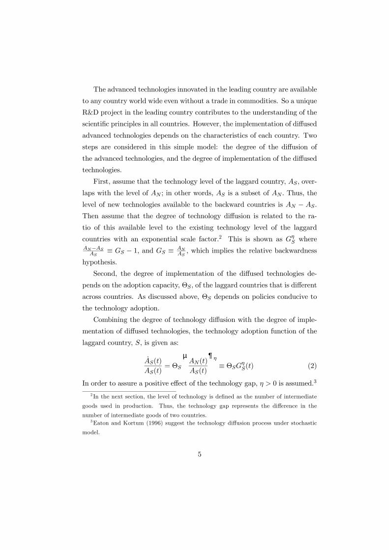
ΘΘΘΘ1G1

g

ΘΘΘΘ2G2

ΘΘΘΘ3G3 E1 E2 E3

gN

0

gN

Θ1

�

��

�

��

gN

Θ2

�

��

�

�� G0

gN

Θ3

�

��

�

�� G ��

�

����

�≡

S

N

AA

Rich Poor

Figure 1: A Simple Catching Up Model

but different levels of adoption capacity. For a constant level of adoption

capacity, ΘS, countries0 growth rates along the transition path and steady

state levels of technology gap, GS , will be ranked by ΘS.

Remark 3 (Economic Policy Implication) If a country caught in an

underdeveloped position can increase its adoption capacity through economic

policies, then this country might move from underdeveloped to the catching

up position. Conversely, if a country in the catching up process has a de-

crease in the level of adoption capacity due to policy failure, then this country

might move from the catching up to the underdeveloped position.

For example, in Figure 1 (with η = 1), E1, E2, and E3 are the steady

state values of the technology gap. Assuming that G0 is the initial technol-

ogy gap, the countries, with the adoption capacities Θ1 and Θ2, are in the

catching up position, and the other country with Θ3 is in an underdeveloped

7

position since the technology gap in E3 is wider than G0. If this country can

increase its adoption capacity from Θ3 to Θ1 or Θ2, it can move from the

underdeveloped to the catching up position.

What happens if two laggard countries start from different technology

gaps? If their adoption capacities are the same, then the country that is

more highly backward will grow faster. However, in reality, these levels are

not the same. Even if one country is highly backward, it cannot grow rapidly

without the support of its adoption capacity. This means that the country

cannot realize and implement advanced technologies sufficiently because of

its limited capacity to do so.

3 A General Equilibrium Model

The simple catching up model operates under the assumptions that the

technological progress of the leading country is given exogenously, and that

the technology adoption process of the laggard countries does not need any

resources. In this section, the simple model is extended by assuming that

the innovation and adoption processes need a resource.

All technological change is assumed to take the form of increases in

the range of intermediate inputs used in production. While new products

are produced through the investment of resources in the leading countries,

they are available to all laggard countries. Since the laggard countries have

different capacities for the adoption and implementation of new technologies,

it is assumed that the real effect of diffused technologies will depend on

the catching up theory previously discussed. As in the simple model, it is

assumed here that there is no trade in commodities.

The extended catching up model is combined with a R&D based endoge-

nous growth model as in those in Romer (1990), Grossman and Helpman

(1991), and Jones (1995). The growth rate of technology and the level of

technology gap in the steady state are then derived.

8

3.1 Producer Behavior

3.1.1 The Þnal goods sector

Assume that the production of Þnal goods Y (t) uses human capital HY (t)

and a collection of intermediate capital inputs xj(t) at any point in time for

two countries � the technological leader (N) and the technological laggard

(S).5

Y (t) = H(t)1−αY

Z A(t)

0xj(t)

αdj (5)

where A(t) is the variety of available intermediate capital inputs, and α is

a parameter between zero and one. While the production of Þnal output

can employ any capital goods indexed by [0,∞), only the available goods,[0, A(t)], at time t are used. The technology in (5) can be accessed by all

agents in each country, and production occurs under a perfectly competitive

market. The total stock of durables is related to capital stock as follows,

K(t) =

Z A(t)

0xj(t)dj = A(t)x(t). (6)

It is assumed that the number of workers, L, is homogenous within a

country, and that each unit of labor has been trained with Sh years of

schooling. Sh is determined by the constant fraction of time individuals

spend in accumulating skills:

HY (t) (≡ hLY (t)) = eωShLY (t) (7)

where h stands for human capital per worker and LY is the labor force em-

ployed in Þnal goods production. The exponential formulation is motivated

by the Mincer wage equation in empirical labor literature.6 It is straight-

forward to show that the parameter ω can be interpreted as the return to

5Subscript i = N and S is omitted without loss of generality .6See Halls and Jones (1999) for details.

9

schooling. Note that ω = 0 is a standard production function with unskilled

labor.

Normalizing the price of Þnal output to 1, the demand for intermediate

input j demanded by a Þrm that manufactures Y units of the Þnal goods

is:

pj(t) = αH1−αY (t)xα−1j (t), j ∈ [0, A(t)] (8)

where pj(t) is the price of jth brand at time t.

The wage rate for human capital is:

wY (t) = (1− α) Y (t)HY (t)

. (9)

3.1.2 The Intermediate Goods Sector

Assume that the intermediate goods sector is composed of an inÞnite number

of Þrms on the interval [0, A(t)], and has purchased a design from the R&D

sector. All differentiated intermediate products are manufactured subject

to a common constant returns to scale under a monopolistic competitive

market structure at any moment of time. A Þrm that has purchased a

design can then effortlessly transform each unit of capital into a unit of

the intermediate input. It is assumed that capital is rented at rate r. A

unique supplier of jth variety who faces the demand function (8) maximizes

operating proÞts at time t.

maxxj(t)

πj(t) = pj(t)xj(t)− rj(t)xj(t) j ∈ [0, A(t)] (10)

Once a Þrm in either region has mastered the technology for some products,

the goods can be manufactured with one unit of capital goods per unit of

output.

A Þrm in the leading country that is uniquely able to produce some in-

novative goods faces competition only from other horizontally differentiated

brands. Such a monopoly Þrm sees the downward sloping demand function

10

in (8) and maximizes proÞts by setting its price at a Þxed markup over unit

cost, given as:

pN(t) =rN(t)

α. (11)

The monopolist realizes sales of xN(t) and earns operating proÞts per

unit of time, πN(t).

πN(t) = (1− α)pN(t)xN(t) (12)

If a Þrm in the laggard country adopts the advanced technology, then it

has monopoly power over this technology. Thus the Þrm could charge its

monopoly price without fear of competition from other Þrms in the same

laggard country. The price and the proÞt functions are:

pS(t) =rS(t)

α(13)

πS(t) = (1− α) pS(t)xS(t). (14)

3.1.3 Innovation and Technology Adoption Function

It is assumed that the introduction of new products and the technology adop-

tion process need a resource. Here the resource is human capital. Based

on Jones (1995), the microfoundations for the innovation and technology

adoption function are technology transfer and externalities arising from du-

plications made in the R&D process.

The change of products introduced by the leader is assumed as,

úAN(t) = φNAψN(t)H

ξAN(t) (15)

where HAN (t) is the human capital employed in technology innovation and

φN is the productivity parameter in the innovation process. In this techno-

logical innovation function, ψ < 0 implies that the rate of innovation falls

with the accumulated level of technology; ψ > 0 corresponds to the positive

11

effect of the stock of technology that has already been discovered. ψ = 0

represents technology innovation that is independent of the stock of accumu-

lated technology.7 In addition, 0 < ξ 5 1 is assumed, which implies that the

duplication of research might reduce the total number of new ideas produced

by HAN . The level of human capital employed in the innovation process is

deÞned as hNLAN(t). hN and LAN(t) are human capital per worker and

labor force employed in R&D in the leading country, respectively.

As described in the simple catching up model, the incentive for the lag-

gard in adopting the advanced technology is that adoption is easier and less

costly than innovation. Combining the adoption capacity and the relative

backwardness hypothesis, the technological adoption process in the laggard

countries is then assumed.

úAS(t) = ΘSGS(t)ηAψS(t)H

ξAS(t) (16)

where ΘS reßects adoption capacity; G is the technology gap; and HAS(t) ≡hSLAS(t) is the human capital employed in technology adoption, and hS is

the labor force efficiency rate LAS(t). Following the technology innovation

function of the leading country, ψ > 0 implies a positive effect of accumu-

lated level of technology, and vice versa. Finally, resources in the leading

country are assumed to be more productive in undertaking innovation than

are resources in the laggard countries, φN > ΘS, and the growth rates of

the labor forces are ni for countries i = N and S.

3.1.4 Free Entry Conditions in the R&D Sector

An entrepreneur who devotes HAN(t) units of human capital in the research

sector for a time interval of length, dt, has the ability to produce new prod-

ucts by (15), i.e., dAN = φNAψN(t)H

ξAN(t)dt. The total cost to produce new

products is wANHAN(t)dt. Assuming no barriers to entry in the R&D sector,

the free entry condition gives:

7For the positive steady state growth rate of technology derived later, ψ < 1 is assumed.

12

wAN (t) = vAN (t)φNAψN(t)H

ξ−1AN (t) (17)

where wAN (t) is the wage rate of the human capital employed in the R&D

sector, and vAN(t) =R∞t e−[r(τ)−r(t)]πN(τ)dτ represents the market value of

each blueprint.

The entrepreneurs in the laggard countries can enter freely into the ac-

tivity of technology adoption. They decide how many and which products to

adopt. Since all products yield identical proÞts by symmetry of the model,

the laggard countries are assumed to choose them randomly among the stock

of AN(t). These are products in the leading country that have not previously

been adopted. Using the same analysis as that used in the leader, the free

entry condition in the adoption process is given by,

wAS(t) = vAS(t)ΘSGη(t)AψS(t)H

ξ−1AS (t) (18)

where vAS(t) is the value of a typical brand and wAS(t) is the wage rate

of human capital in the technology adoption sector. This relationship, like

(17), limits the value of a Þrm to the cost of market entry.

3.1.5 The No-arbitrage Condition

The Þrm in country i = N,S earns proÞts, πi(t)dt, for a product produced

during the length of time dt, and realizes a capital gain (or loss) of úvAi(t)dt.

The no�arbitrage condition implies that the total return on equity claims

must equal the opportunity cost, ri(t), of the invested capital:

πi(t)

vAi(t)+úvAi(t)

vAi(t)= ri(t). (19)

3.1.6 The Factor Market Clearing Condition

While the human capital involved in the manufacturing sector of the Þnal

goods in the leading country isHY N(t) units,·

úAN (t)

φNAψN (t)

¸ 1ξ

units are employed

13

in the research sector from (15). Labor market equilibrium in the leading

country requires that

"úAN (t)

φNAψN(t)

# 1ξ

+HY N(t) = HN(t) (20)

where HN (t) is the supply of human capital in the leading country. Since

human capital is deÞned as hNLN(t), (20) is the same as LAN(t)+LY N (t) =

LN(t).

Similarly, for the laggard countries,

"úAS(t)

ΘSGη(t)AψS(t)

# 1ξ

+HY S(t) = HS(t). (21)

3.2 Consumer Behavior

Suppose consumers share identical preferences and maximize utility over an

inÞnite horizon where the utility function has a constant intertemporal elas-

ticity of substitution, 1σ . The consumer0s intertemporal optimization prob-

lem for both of the countries is to maximize utility subject to intertemporal

budget constraints over an inÞnite horizon.

max{c(t)}

U0 =

Z ∞

0e−ρtL(t)

c(t)1−σ − 11− σ dt (22)

s.t úK(t) = r(t)K(t) +w(t)(1− Sh)L(t) +Aøπ − c(t)L(t) (23)

where ρ represents the subjective discount rate and c(t) is an index of con-

sumption per worker at time t. It is assumed that ρ is constant. Households

can borrow or lend freely at the instantaneous interest rate r(t), w(t) is the

wage rate, and K(t) is the total capital stock. Here Sh is the constant frac-

tion of time individuals spend in accumulating skills, and øπ is the monopoly

proÞt in the intermediate goods sector.

14

The maximization of utility (22) subject to budget constraint (23) yields:

úc(t)

c(t)=1

σ(r(t)− ρ). (24)

3.3 Steady State Analysis

3.3.1 The Steady State Growth Rate

It is easily shown that the growth rate of output per capita and consumption

per capita in the steady state are equal to the growth rate of technology,

i.e., introduction of new goods at each time period. Since the growth rate of

researchers must be equal to the growth rate of the population in the steady

state, the steady state growth rate is:

g = gy = gc = gA =nξ

1− ψ (25)

where n is population growth rate and y is output per worker. The param-

eter, ψ, should be less than 1 to get a stable solution, implying a positive

growth rate in the steady state.8

The steady state growth rate is determined by the parameters for the

technology adoption (or innovation) function, ψ, and the growth rate of

researchers in technology adoption (or innovation), n, which is the same as

the population growth rate. Thus, the growth rate in the steady state is

independent of the scale effect as shown in Jones (1995). Next, the level of

the technology gap and the relative level of the Þnal output per worker in

the steady state are derived.

3.3.2 The Steady State Technology Gap

First, combining (15) and (16), the steady state technology gap is:8Since the steady state growth rate of technology gap is not zero if two population

growth rates are not the same, the steady state growth rates of technology will be gN =ξnN1−ψ and gS = ξ(nNη+(1−ψ)nS)

(1−ψ+η)(1−ψ) , where nN and nS are the population growth rates of two

countries, respectively.

15

G∗ =µgSφNgNΘS

¶ 11−ψ+η

µH∗AN

H∗AS

¶ ξ1−ψ+η

. (26)

This indicates that the steady state technology gap depends on the relative

steady state growth rate and human capital stock invested in the innovation

and adoption process. Then following the steps below, H∗AN and H∗

AS are

derived.

Substituting the demand for intermediate goods, (8), into the proÞt func-

tion, (12):

πN(t) = (1− α)pN(t)xN(t) = α(1− α) YN (t)AN(t)

(27)

where YN(t) = AN(t)H1−αY (t)xαN(t) by symmetry of the model.

Since the steady state growth rate of consumption per worker is con-

stant by (25) and the parameters, σ and ρ, are assumed as constants, rN is

constant in the steady state. The equations (8), (11), and (12) imply:

úπN(t)

πN(t)= nN . (28)

Since it is assumed that the population growth rate is constant, the

growth rate in the value of patent, vN(t), is constant by (19) and the fact

that rN is constant. Thus the following is derived by (19) and (28)

úπN (t)

πN (t)=úvAN(t)

vAN(t)= nN . (29)

Combining (19), (27), and (29),

vAN(t) =α(1− α)rN(t)− nN

YN(t)

AN(t). (30)

Since the wage rate in the Þnal goods sector is the same as that in the

R&D sector by free mobility of the labor force, then:

(1− α) YN(t)HY N(t)

= vAN(t)úAN(t)

HAN(t). (31)

16

Combining (15) or (16) and full employment condition, (20) or (21) with

(31), the steady state value of HAi for i = N and S by symmetry is:

H∗Ai =

αgiHiαgi + ri(t)− ni . (32)

Substituting (32) into (26),

G∗S(t) =µgSφNgNΘS

¶ 11−ψ+η

µHNgN (αgS + rS − nS)HSgS (αgN + rN − nN)

¶ ξ1−ψ+η

. (33)

Since the technology growth rates in the steady state and the interest

rates are the same across countries under the assumption of same population

growth rate across countries:

G∗S(t) =µφNΘS

¶ 11−ψ+η

µHN(t)

HS(t)

¶ ξ1−ψ+η

. (34)

Since ψ < 1 and η > 0, 1 − ψ + η is positive. The technology gapin the steady state will depend on relative human capital stock, adoption

capacity of the laggard countries, and the productivity parameter for the

R&D sector in the leading country. Given the level of adoption capacity,

the countries that have a higher level of human capital stock have a higher

level of technology, implying a decrease in the steady state technology gap.

The steady state technology gap gives the general equilibrium version

of the simple catching up model in section 2, and the remarks made in

the simple model remain valid in this general equilibrium model setup as

well. First, the laggard country cannot reach the technology level of the

leading country unless it has a high adoption capacity or a large human

capital stock. Thus, countries with small human capital should increase their

adoption capacity. Second, a government can increase the technology level

by improving adoption capacity through policies conducive to technology

adoption.

In addition, the symmetric aggregate production function and the de-

mand functions for intermediate goods lead to the following steady state

17

output per worker:

y∗Ny∗S

=hY NhY S

öpG∗ (35)

where öp ≡³pSpN

´ α1−α

.

Substituting the steady state value of the technology gap, (34), the fol-

lowing relative output per worker in the steady state is derived.

y∗Ny∗S

= öphY NhY S

µgSφNgNΘS

¶ 11−ψ+η

µHNgN (αgS + rS − nS)HSgS (αgN + rN − nN)

¶ ξ1−ψ+η

(36)

The relative output per worker is affected by relative population growth

rate, relative steady state growth rate and relative human capital stock.

As Jones (1999) summarizes, this result holds for other endogenous growth

models if the steady state technology stock depends on the human capital

stock invested in the technology progress.

Under the assumption of the same population growth rates across coun-

tries,

µyN (t)

yS(t)

¶∗=hY NhY S

µφNΘS

¶ 11−ψ+η

µHNHS

¶ ξ1−ψ+η

. (37)

Given the adoption capacity and a high human capital per worker, a

larger labor force leads to a higher GDP per worker. While a larger la-

bor force can increase the output per worker given the human capital per

worker, its increase with the support of the adoption capacity makes this

increase of the real GDP per worker more effective. China and India, which

have large labor forces, are not guaranteed to have high levels of GDP per

worker because a larger labor force is not the same as a high level of human

capital, which is the input for producing Þnal goods and adopting advanced

technologies. Thus, even if the relative output per worker depends on the

relative labor force between two countries, the level of adoption capacity and

18

the efficiency of human capital should be supported to get higher output per

worker as well.9

4 The Empirical Tests

Based on the catching up theories described in sections 2 and 3, this section

analyzes the association between the growth rate of TFP and the factors

that affect the level of adoption capacity by using regression analyses. The

approximate speeds of technological catching up and their standard errors

are also derived.

4.1 Total Factor Productivity (TFP)

Substituting (6) and (7) into the production function, (5), the Cobb�Douglas

form of the production function with respect to physical and human capital

is derived.

Yi(t) = Ki(t)α(Ai(t)Hi(t))

1−α (38)

After equation (38) is divided by labor force, the levels and growth rates

of TFP are derived. Following Psacharopoulos (1994) and Hall and Jones

(1999), the estimates of the rates of the return to schooling are used. For the

Þrst 4 years of education, the rate of return is 13.4 percent, and for the next

4 years and beyond 8 years, these are 10.1 and 6.8 percent, respectively. The

data for real GDP per worker and the labor force are from Heston�Summer

Mark 5.6. Sh is assumed as the average years of secondary schooling, which

is from Barro�Lee (1996). Capital stock is derived by using the perpetual

inventory method. The initial value of the 1960 capital stock is derived byI60g+δ where I60 is the investment rate in 1960 and g is the average growth

9While the theoretical models assume that human capital per worker, h, is constant

across countries, this is relaxed in empirical tests with the efficiency of the average years

of secondary schooling.

19

rate from 1960 to 1970 of the investment series. The depreciation rate, δ, is

assumed as 6 percent, and that α = 1/3 is also assumed.

4.2 Estimation

4.2.1 Model

Let G∗S(t) be the steady-state level of the technology gap given by (4) in the

simple catching up model and (34) in the general equilibrium model, and

let GS(t) be the actual value of the technology gap between the leading and

the laggard countries.

First, the technology adoption function, (16), is approximated by using a

log linearization with a Þrst order Taylor series expansion around the steady

state value of the technology gap.

d lnAS(t)

dt∼= g + ηg [lnGS(t)− lnG∗S ] + (ψ − 1)g(lnAS − lnA∗S)

+g [lnHAS(t)− lnH∗AS] (39)

where g is the steady state growth rate of TFP.

Similarly, the technology innovation function of the leading country is

approximated as:

d lnAN(t)

dt∼= g + (ψ − 1)g(lnAN − lnA∗N) + g [lnHAN(t)− lnH∗

AN ] . (40)

Subtracting (39) from (40):

d lnAN(t)

dt− d lnAS(t)

dt∼= − λ [lnGS(t)− lnG∗S ]− g [lnHAS(t)− lnH∗

AS ]

+g(lnHAN − lnH∗AN) (41)

where λ ≡ (1 − ψ + η)g. Since the growth rate and the technology level ofthe leading country are constant through the equation, λ is the speed of

20

technological catching up of the laggard countries. This shows how rapidly

the actual technology gap between the leading and the laggard countries

approaches its steady state value each year.

Since d lnG(t)dt = d lnANdt − d lnAS(t)

dt , (41) is integrated from t = 0 to t = T,

Z T

0

µd lnG(t)

dt+ λ lnGS(t)

¶eλtdt =

λ lnG∗Z T

0eλtdt+ ηg

Z T

0eλt lnHANdt− ηg lnH∗

AN

Z T

0eλtdt

−gZ T

0eλt lnHASdt+ g lnH

∗AS

Z T

0eλtdt. (42)

Using the total human capital stock instead of the human capital stock

employed in technology innovation and adoption process, the integration

leads to the following regression equation.10

lnAS(T )− lnAS(0)T

= constant+ β lnGS(0)− β lnG∗S+gβ

λ[lnhS + lnLS(0)]− gβ

λlnH∗

S + ξS (43)

where all variables for the leading country are constant, and β = 1−e−λTT ,

and ξS is a residual of regression.

Since the relative backwardness in the steady state, (34), is a negative

function of the adoption capacity and human capital of the laggard country,

and assuming that the level of adoption capacity is determined by the factors

listed in the next subsection, the following regression equation is used.

Gtfp7089S = constant + β lnGS(0) +IX

m=0

αm lnBmS (0) + γ lnLS(0) + ξS

(44)

where Gtfp7089S and GS(0) imply the growth rate of TFP from 1970 to

1989 and the technology gap in 1970 of country S, respectively, and BmS (0)

10The derivation is available on request.

21

reßects the mth determinant of the adoption capacity of country S in 1970.

Population as one of the independent variables is based on the production

function (38) and the technology adoption function of the laggard countries

(16), and γ reßects gβλ . Here the regression equations divide human capital

stock into population size, LS, and human capital per worker, hS , following

equation (7). The technology gap is deÞned as TFP gap where the United

States is the leading country.11

4.2.2 Data

Policy variables and the income distribution index are used as approximate

indicators of adoption capacity.12 Due to a lack of data availability, only a

limited number of variables are used.

First, the variable chosen to represent human capital is the average years

of secondary schooling. These data come from Barro and Lee (1996).13

Second, the black market premium (BMP) has been used as a measure

of exchange control or government trade policy. This measure reßects the

degree of the distortion of the foreign exchange market. In this analysis the

data available for use, which comes from Collins and Bosworth (1996) are

the average values from 1970 to 1980.

Third, two openness indices have been used. It is assumed that these

indices reßect the openness to foreign competition. The Þrst index is deÞned

as the average value of the ratio of the sum of exports and imports to GDP

in current international prices from 1960 to 1969 (Penn World Tables 5.6).

This is denoted as Openness as in the regression results. For the second

one, the Sachs and Warner (1996) index (Openness SW) in 1970 is used

11 It can be assumed that the leading country is G7 or a group of developed countries

which are on the frontier of some technologies.12The effect of economic policies on economic growth is discussed in Abramovitz (1995),

Abramovitz and David (1996), Collins and Bosworth (1996), and Jones (1998b).13Benhabib and Spiegel (1994) argue that human capital contributes to productivity

by facilitating the adoption and implementation of new technologies rather than causing

economic growth directly.

22

as an alternative proxy for the degree of openness. This proxy is deÞned

as a dummy variable: 1 for open economies and 0 if a country is closed.14

Because the Sachs-Warner openness index includes BMP by deÞnition, this

variable is excluded in the regressions.

Fourth, the ratio of gross claims on the private sector by central and

deposit banks to GDP is used to represent the domestic Þnancial status.

This factor reßects the overall size of the public sector including the degree of

public sector borrowing, thus, implying a broad array of Þnancial indicators.

The index used is fromKing and Levine (1993) and denoted as Finance in the

regressions. McKinnon (1973) and Shaw (1973) found a positive relationship

between Þnancial development and economic growth, and King and Levine

(1993), and Levine and Zervos (1998) show that the Þnancial systems are

both positively and robustly correlated with productivity growth and capital

accumulation, as well as, economic growth.

Fifth, the Gini coefficient is included as an approximation of income

inequality in the society. These data come from Deininger and Squire (1996).

Income inequality may be harmful to economic growth because the concerns

about social and political conßict are more likely to lead to government

policies that hinder growth.

Lastly, in order to test the scale effects on the technological adoption

process, the population size used is from the Penn World Tables 5.6.

The mean and variance of the dependent and independent variables are

summarized in Table 1. All variables except the TFP growth rate and human

capital are in log form and BMP is deÞned as the log of (1+ black market

premium).

14 It is equal to 0 if a country scored a 1 on either the BMP, the SOC (dummy variable

equals 1 if the country was classiÞed as socialist), the EXM variable (dummy variable

equals 1 if a country had a score of 4 on the export marketing index), or the OWQID

(dummy variable equals 1 if OWQI>0.4). OWQI indicates coverage of quotas on imports

of intermediate and capital goods.

23

Table 1. Summary Statistics of Adoption Capacity Determinants

Variables MeanStandard

DeviationMin Max

Growth Rate

of TFP0.0016 0.0142 - 0.0421 0.0235

TFP

gap0.6850 0.4401 - 0.2429 1.8290

Openness - 0.8870 0.6080 - 2.3230 0.9761

Human 0.4580 0.1840 0.0042 0.8181

BMP 0.1511 0.2771 0.0000 1.6730

Finance - 1.7770 0.8023 - 4.8940 0.0276

Gini - 0.9081 0.2479 - 1.3820 - 0.3567

Population 9.1760 1.4418 5.4760 13.2100

4.2.3 The Regression Results

All regression coefficients are estimated by OLS and the results are reported

in Table 2. Data availability reduces the sample size to 67 in the Þrst two

models and 66 in other models.15 The empirical results strongly support the

catching up theory. The technology gap, which is conditional on the factors

of adoption capacity, is signiÞcantly correlated with the TFP growth rate.

Furthermore, the robust role of country size is found.

A simple relation between TFP growth rate and the degree of relative

backwardness is Þrst estimated.16 The technology gap is not signiÞcant

and R2 is almost zero, suggesting the rejection of an absolute technological

catching up. Thus, the relative backwardness alone is not sufficient to catch

up with the technology of the leading country. The correlation between the

15Collins and Bosworth (1996) show the contribution of TFP growth through growth

accounting for East Asia and test the association between growth of output per worker

(and capital accumulation and TFP growth) and macroeconomic policy variables.16The estimated coefficient for initial gap is 0.0049 (t statistic= 1.3823) and R2 is 0.02.

24

0.0 0.5 1.0 1.5 2.0

-0.0

4-0

.02

0.0

0.02

Gap of TFP 1970

Gro

wth

Rat

e of

TFP

70-

89

Figure 2: Growth Rate and Gap of TFP (70-89)

TFP growth rate and the degree of relative backwardness is shown in Figure

2 with the regression line. Thus, the respective adoption capacity should be

considered.

Models (I) and (II) show the effect of the degree of openness, human

capital, gini coefficient, Þnancial development and the country size on the

TFP growth rate. The Þrst openness variable is not signiÞcant. Openness

is interpreted as the factor which promotes technology transfer even if the

general equilibrium model of this paper ignores the trade in commodities.

However, this result should be interpreted carefully. The openness might not

reßect the complete ßow of new ideas or technology through trade because

this deÞnition includes all kinds of trade, for example, agricultural goods

that are not sensitive to technological transfer.

The empirical results produced by using a different openness index, i.e.,

25

Sachs-Warner index, are presented in Models (III) and (IV). Openness is

signiÞcant in the speciÞcations. However, the results might come from dif-

ferent interpretations of openness. The deÞnition of this index takes into

account the black market premium and quota index. Thus, the implication

is different from the openness index in the Penn data that considers the

simple average ratio of the exports and imports to GDP.

Model (II) shows the effect of the black market premium. As it was

interpreted in previous section, BMP is the degree of distortion of the foreign

exchange market. This variable plays a signiÞcant role in explaining the

TFP growth rate, which implies that the foreign exchange market should

be included in explaining the technological adoption process. Since the

black market premium is considered as one of determinants of the Sachs

and Warner openness index, this is excluded in regressions (III) and (IV).

The effect of the domestic Þnancial development is found in models (I),

(II), and (IV). While the Þrst two models show the robust correlation be-

tween the Þnancial system and TFP growth rates, the other model does

not.17

All models include the gini coefficient as an equity factor and human

capital variable. The human capital is signiÞcant in all models, the same

as the results in the empirical growth models of Barro (1991), and Mankiw,

Romer and Weil (1992) etc. Except in the second model, the role of income

distribution is not signiÞcant. The second model shows that the explanatory

power of the Gini coefficient is almost the same as that of the initial gap.18

Income distribution is known as a trade off with economic growth. How-

17Even with a different deÞnition of Þnancial development (the ratio of the liquid liabil-

ities of a Þnancial system to GDP from King and Levine), the regression results are the

same.18Recent empirical works tend to support a negative relationship, that the greater a

society0s income inequality is the slower its growth. Perrson and Guido (1994) Þnd a

strong negative relationship between income inequality and growth in GDP per head.

Furthermore, Perotti (1996) supports these predictions through diverse channels such as

fertility, investment in education, Þscal policy, and sociopolitical instability.

26

ever, these empirical results suggest more research is needed on the relation

between equity factor and TFP growth rates.

Surprisingly, we found that the role of population is signiÞcant. All

regression coefficients on the level of population are strongly signiÞcant at

the 5% signiÞcance level. Supporting the deÞnition of the technological

adoption function in the theoretical framework, the results suggest that

the human capital investment in the R&D sector plays a signiÞcant role in

increasing the implementation and adoption of advanced technologies.

4.2.4 The Robustness of Scale Effects

Table 3 reports the results of robustness tests of scale effect. The second

model speciÞcation of Table 2 is used as the base because this includes all

possible combinations of the independent variables used in the empirical

tests. The other speciÞcations do not affect the results of robustness tests

as well.

Before we go over the regression tests, the TFP level and growth rate are

compared with Klenow and Rodrigues-Clare (1997). To get the correlation

for the same year, the TFP level at 1985 is derived as well by using the same

method in paper. The correlation coefficient between the two TFP levels at

1985 is 0.96. For the two growth rates, while their given growth rates cover

the years 1960 to 1985, this paper covers 1970 to 1985. The correlation

coefficient of the two growth rates is 0.87.

Going over the regression results, the White heteroskedastic-consistent

estimate, which tests the inconsistency of the estimated coefficients, is re-

ported. This estimation computes standard errors that are consistent even

in the presence of unknown heteroskedasticity. The estimated coefficient

does not affect the signiÞcant role of population.

SpeciÞcation B tests the effects of outliers. The outliers are identiÞed

through residual plots, Cook�s distance, and partial regression plots for pop-

ulation. Even after the outliers (Uganda, Guyana and Iran) are removed,

27

the coefficient on the population is 0.0039 which is not much different from

the results in the original models.

Third, to consider the sample selection bias, different sample sizes are

used by removing independent variables having a small sample. Here the

number of the maximum sample is 91 excluding Gini coefficient, BMP and

Þnancial development. However, it does not affect the explanatory power of

the population either.

Next, the two model speciÞcations take account of the missing variable

bias problem. Except for the determinants in the main empirical speciÞ-

cations, several variables are then selected. These are the distance from

the equator and the fraction of population speaking English as a mother

tongue, which might reßect the effect of Western European expansion in

World history.

SpeciÞcation D includes the distance from the equator as another in-

dependent variable which is measured as the absolute value of latitude in

degrees divided by 90 as in Hall and Jones (1999). It is widely known that

economies further from the equator are more successful. In addition, speci-

Þcation E includes the fraction of population speaking English as a mother

tongue, and the distance from the equator. This reßects that familiarity

with English might inßuence the process of technology transfer. These two

different speciÞcations show that there is little change in the coefficient of

the country size. The data of latitude and language are from Hall and Jones

(1999).

Finally, by including the population size as one of the independent vari-

ables, two different model speciÞcations as in Barro (1991) and Mankiw,

Romer, and Weil (1992) are estimated, even if the dependent variable is

the growth rate of income per capita. The coefficient on population level is

not guaranteed to be signiÞcant, reßecting that the effect of population on

economic growth is an unresolved problem and suggests more work in the

future. For Mankiw, Romer and Weil, the population growth rate and level

28

are not signiÞcant at the 5% signiÞcance level. However, the model speciÞ-

cations without human capital show the more signiÞcant role of population

than that of population growth rate. For Barro speciÞcations, the results

are sensitive to the combinations of independent variables. It is concluded

that while the regression with the government expenditure share to GDP as

one of the independent variables does not show the role of population to be

signiÞcant, those with an investment share to GDP do show a strong role.

As several robustness tests show above, the effect of the population level

might be sensitive to the model speciÞcations and more research on the role

of country size is suggested.

4.2.5 The Speeds of Technological Catching Up

The speed of technological catching up, λ, in equation (41) shows how

rapidly the TFP gap approaches its steady state value. The value of speed

is derived by using the coefficient on the initial technology gap of regression

equation (44) since β = 1−e−λTT in equation (43). In addition to the speeds

of technological catching up, their standard errors are derived by assuming

that the coefficients for the initial technology gap follow normal distribution,

with mean, ÷β, and variances, σ2�β. Taking linearization of β around the mean,

E[β] = ÷β,

λ ∼= 1

1− ÷βT (β −÷β). (45)

Since ÷β is a coefficient for the initial technology gap and T is 19, λ

follows normal distribution with mean, 0, and variance,h

11−�βT

i2σ2�β. Using

the regression results in Table 2, the speeds of TFP catching up and their

standard errors are reported in Table 4.

The speeds of TFP catching up are from 1.7 to 2.4 percent, which imply

similar speeds to those for GDP per capita derived by Mankiw, Romer and

Weil (1992). Finally, assuming around 2% speed of TFP catching up, the

economy moves halfway to a steady state in about 35 years.

29

5 Conclusion

Based on the recent empirical Þndings that the technology levels and growth

rates are different across countries, this paper suggests the simple and ex-

tended catching up models. These models show how the innovation in the

leading countries are adopted by the laggard countries. Combining the ex-

tended catching up model with the R&D based endogenous growth models,

the theoretical model demonstrates that even if the steady state growth

rates of the technology of two countries are independent of the scale effect,

the steady state relative backwardness depends on the level of adoption ca-

pacity, the productivity of the R&D sector, and the relative human capital

stock.

Supporting the predictions from the models, the empirical results show

that the technology catching up occurs even without the diminishing marginal

productivity of capital. Since TFP is one component of real GDP per worker,

the extended version of the catching up theory suggests that the channel of

TFP catching up might constitute one of the major forces for the conditional

convergence process of real GDP per worker.

It is shown that the policies for building adoption capacity are very

important. These policies include human capital, Þnancial development,

exchange rate policy and so on. If the government succeeds in improving

adoption capacity, it might escape underdevelopment and move into the

catching up process. If the level of adoption capacity falls because of policy

failure, a country even in the catching up process might slide back to the

state of underdevelopment.

Contrary to the recent empirical results that reject the role of population,

the robust role of country size is found. In order to test the robustness of the

empirical results, several tests are taken. They are regressions with different

combinations of independent variables as well as without outliers identiÞed

by diagnostic plots and partial regressions. Thus, the possible problems

of sample selection bias, and outliers do not affect the main conclusions

30

of this paper. The comparisons with the results of the recent empirical

speciÞcations, however, show that the robust role of population in growth

rate of real GDP per capita cannot be strongly accepted. With these results,

this paper concludes that the scale effect is an unresolved problem and more

work on this should be done in the future.

The estimated speed of technological catching up is around 2%, implying

that the actual technology gap moves halfway to the steady state technol-

ogy gap in about 35 years. Finally, the general equilibrium model does not

allow trade in commodities. Since trade in commodities is one of the im-

portant channels for transferring advanced technologies, this factor needs

to considered in future research. Furthermore, the factors affecting adop-

tion capacity include institutional factors in addition to human capital and

policy variables. Hence, these indicators should also be considered as well.

31

References

[1] Abramovitz, Moses (1986), �Catching Up, Forging Ahead, and Falling

Behind,� Journal of Economic History, 46, 385-406.

[2] Abramovitz, Moses (1995), �The Element of Social Capability,� In So-

cial Capability and Long�Term Economic Growth, (ed. Bon Ho Koo

and Dwight H. Perkins), St. Martin�s Press.

[3] Abramovitz, Moses and Paul David (1996), �Convergence and Deferred

Catch Up: Productivity Leadership and the Waning of American Ex-

ceptionalism,� In The Mosaic of Economic Growth, (ed. R. Landau, T.

Taylor and G. Wright), Stanford University Press.

[4] Barro, Robert J. (1991), �Economic Growth in a Cross Section of Coun-

tries,� Quarterly Journal of Economics, 106(2), 407�443.

[5] Barro, Robert J. and Xavier Sala�i�Martin (1997), �Technological Dif-

fusion, Convergence, and Growth,� Journal of Economic Growth, 2 (1),

1�26.

[6] Benhabib, Jess and Mark M. Spiegel (1994), �The Role of Human Capi-

tal in Economic Development: Evidence from Aggregate Cross-Country

Data,� Journal of Monetary Economics, 34(2), 143-173.

[7] Bernard, Andrew B. and Charles I. Jones (1996a), �Productivity across

Industries and Countries: Time Series Theory and Evidence,� Review

of Economics and Statistics, 135-146.

[8] Bernard, Andrew B. and Charles I. Jones (1996b), �Comparing Ap-

ples to Oranges: Productivity Convergence and Measurement Across

Industries and Countries,� American Economic Review, 86, 1216-1238.

[9] Collins, Susan M. and Barry P. Bosworth (1996), �Economic Growth

in East Asia: Accumulation versus Assimilation,� Brookings Papers on

Economic Activity (2), 135�203.

32

[10] Deininger, Klaus and Lyn Squire (1996), �A New Data Set Measuring

Income Inequality,� World Bank Economic Review 10 (3), 565-591.

[11] Eaton and Kortum (1996),�Trade in Ideas: Patenting and Productivity

in the OECD,� Journal of International Economics, 40, 251-278.

[12] Grossman, Gene M., and Elhanan Helpman (1991), Innovation and

Growth in the Global Economy, Cambridge, Mass.: MIT press.

[13] Gershenkron, Alexander (1952), �Economic Backwardness in Histori-

cal Perspective,� In The Progress of Underdeveloped Areas, (ed. B.F.

Hoslitz), Cambridge: Harvard University Press.

[14] Hall, Robert and Charles Jones (1999), �Why Do Some Countries Pro-

duce So Much More Output per Worker than Others?,� Quarterly Jour-

nal of Economics, 114, 83-116.

[15] Jones, Charles I. (1995), �R&D Based Models of Economic Growth,�

Journal of Political Economy, 103, 759�784.

[16] Jones, Charles I. (1998a), �Sources of U.S. Economic Growth in a World

of Ideas,� mimeo, Stanford University.

[17] Jones, Charles I. (1998b), �Population and Ideas: A Theory of Endoge-

nous Growth,� mimeo, Stanford University.

[18] Jones, Charles I. (1999), �Growth: With or Without Scale Effect,�

American Economic Review Papers and Proceedings, 89, 139-144.

[19] Kang, Sung Jin and Yasuyuki Sawada (1997), �Financial Repression

and External Openness in an Endogenous Growth Model,� mimeo,

Stanford University.

[20] King, Robert G. and Ross Levine (1993), �Finance and Growth: Schum-

peter Might Be Right,� Quarterly Journal of Economics, 108(3), 717�

737.

33

[21] Klenow, Peter J., Andrés Rodríguez-Clare (1997), �The Neoclassical

Revival in Growth Economics: Has It Gone Too Far?,� NBER Macroe-

conomics Annual, 73-114.

[22] Levine, R. and S. Zervos (1998), �Stock Market, Banks, and Economic

Growth,� American Economic Review 88, 537-558.

[23] Mankiw, N. Gregory, Romer, David, and Weil, David N. (1992), �A

Contribution to the Empirics of Economic Growth,� Quarterly Journal

of Economics, 407-37.

[24] McKinnon, Ronald I. (1973), Money and Capital in Economic Devel-

opment, Brookings Institution, Washington D.C..

[25] Parente, Stephen L. and Edward C. Prescott (1994), �Barriers to Tech-

nology Adoption and Development,� Journal of Political Economy, 102,

298-321.

[26] Perotti, Roberto (1996), �Growth, Income Distribution, and Democ-

racy: What the Data Say,� Journal of Economic Growth, 1, 149-187.

[27] Persson, Torsten, and Guido Tabellini (1994), �Is Inequality Harmful

for Growth? Theory and Evidence,� American Economic Review, 84,

600-621.

[28] Romer, Paul (1990), �Endogenous Technological Change,� Journal of

Political Economy, 5, S71�S102.

[29] Sachs, Jeffrey D. and Andrew Warner (1995), �Economic Reform and

the Process of Global Integration,� Brookings Papers on Economic Ac-

tivity, 1, 1�118.

[30] Shaw, Edward S. (1973), Financial Deepening in Economic Develop-

ment, Oxford University Press, New York.

34

[31] Solow, Robert M., (1956), �A Contribution to the Theory of Economic

Growth,� Quarterly Journal of Economics, LXX, 1�25.

[32] Veblen, Thorstein B. (1915), Imperial Germany and the Industrial Rev-

olution, London: Macmillan.

35

Table 2. TFP Growth Rates and Policy Determinants

I II III IV

constant

-

- 0.0548

(- 4.1951)

- 0.0563

(- 4.4647)

- 0.0543

(- 4.9237)

- 0.0478

(- 4.2095)

Initial Gap

-

0.0170

(4.3429)

0.0193

(4.9378)

0.0146

(4.1490)

0.0167

(4.5935)

Openness

-

0.0021

(0.6249)

0.0018

(0.5450)

Openness

(SW)

0.0126

(3.8488)

0.0105

(3.0622)

Human

-

0.0325

(3.3400)

0.0309

(3.2838)

0.0264

(2.7779)

0.0241

(2.5518)

BMP

-

- 0.0124

(- 2.3465)

Finance

-

0.0055

(2.6944)

0.0048

(2.3813)

0.0037

(1.8401)

Gini

-

- 0.0108

(- 1.8480)

- 0.0136

(- 2.3593)

- 0.0036

(- 0.6101)

- 0.0044

(- 0.7650)

Population

-

0.0035

(2.4876)

0.0033

(2.4500)

0.0027

(2.9601)

0.0027

(3.0331)

R2 0.46 0.50 0.50 0.53

sample 67 67 66 66

Note: t-statistics are in parentheses.

36

Table 3. Robustness Tests of Population Size

TFP Gap PopulationNew

VariableR2

A (robust)0.0196

(3.4601)

0.0035

(2.5423)0.51

B (outlier)0.0158

(3.7319)

0.0039

(2.9500)0.48

C (sample)0.0141

(4.5206)

0.0033

(2.5875)0.40

D (latitude)0.0298

(3.0861)

0.0035

(2.5495)

0.0298

(3.0861)0.47

E (English)0.0202

(5.1283)

0.0030

(2.2067)

- 0.0060

(- 1.2155)0.50

Note: t-statistics are in parentheses.

Table 4. The Speeds of TFP Catching Up

Coefficients (β)Standard

Error (β)Speed (λ)

Standard

Error (λ)

Model I 0.0170 0.0039 0.0205 0.0058

Model II 0.0193 0.0039 0.0240 0.0062

Model III 0.0146 0.0035 0.0171 0.0048

Model IV 0.0167 0.0036 0.0201 0.0053

37