CHAPTER 4

REINFORCEMENT LEARNING ApPROACHES

FOR SOLUTION OF

UNIT COMMITMENT PROBLEM

4.1 Introduction

Unit Commitment Problem (UCP) in power system refers to the problem of

determining the onJ off status of generating units that minimize the operating cost

during a given time horizon. Formulation of exact mathematical model for the same is

difficult in practical situations. Cost associated with the different generating units is

also different and random. Most often it is difficult to obtain a precise cost function for

solving UCP. Also availability of the different generating units is different during each

time slot due to the numerous operating constraints.

The time period considered for this short term scheduling task varies from 24

hours to one week. Due to the large number of ON IOFF combinations possible, even

for small number of generating units and short period of time, UCP is a complex

optimization problem. Unit Commitment has been formulated as a non linear, large -

scale, mixed integer combinational optimization problem (Wood and Wollenberg

[2002]).

From the review of the existing strategies, mainly two points can be concluded:

(i) Conventional methods like Lagrange Relaxation, Dynamic Programming etc.

fmd limitation for higher order problems.

(H) Stochastic methods like Genetic Algorithm, Evolutionary Programming etc.

have limited computational efficiency when a large number of units involved.

79

Cliapter4

Since Reinforcement Learning has been found to be a good tool for many of

the optimization problems, it appeared to be very much promising to solve this

scheduling problem using Reinforcement Learning.

In this chapter, a stochastic solution strategy based on Reinforcement Learning

is proposed. The class of algorithms is termed as RL _ VCP. Two varieties of

exploration methods are used: e greedy and pursuit method. The power generation

constraints of the units, minimum up time and minimum down time are also considered

in the formulation of RL solution. A number of case studies are made to illustrate the

reliability and flexibility of the algorithms.

In the next section, a mathematical formulation of the Unit Commitment

Problem is given. For developing a Reinforcement Learning solution to Unit

Commitment problem, it is formulated as a multi stage decision making task. The

Reinforcement solution to simple Unit Commitment problem is reviewed (RL_VCPI).

An efficient solution using pursuit method without considering minimum up time and

minimum down time constraints is suggested (RL _ UCP2). Then the minimum up time

and down time constraints are incorporated and a third algorithm (RL_UCP3) is

developed to solve the same. To make the solution more efficient one, an algorithm

with state aggregation strategy is developed (RL_UCP4).

4.2 Problem Formulation

Unit Commitment Problem is to decide which of the available units has to be

turned on for the next period of time. The decision is subject to the minimization of

fuel cost and to the various system and unit constraints. At the system level, the

forecasted load demand should be satisfied by the units in service. In an interconnected

system, the load demand should also include the interchange power required due to the

contractual obligation between the different connected areas. Spinning reserve is the

other system requirement to be satisfied while selecting the generating units. In

addition, individual units are likely to have status restrictions during any given time

period The problem becomes more complicated when minimum up time and down

80

~forcement LearningApproacfies for Sofution ofVnit Commitment (fro6fem

time requirements are considered, since they couple commitment decisions of

successive hours.

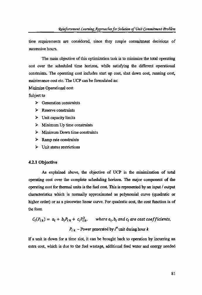
The main objective of this optimization task is to minimize the total operating

cost over the scheduled time horizon, while satisfying the different operational

constraints. The operating cost includes start up cost, shut down cost, running cost,

maintenance cost etc. The uCP can be formulated as:

Minimize Operational cost

Subject to

~ Generation constraints

~ Reserve constraints

~ Unit capacity limits

~ Minimum Up time constraints

~ Minimum Down time constraints

~ Ramp rate constraints

~ Unit status restrictions

4.2.1 Objective

As explained above, the objective of UCP is the minimization of total

operating cost over the complete scheduling horizon. The major component of the

operating cost for thermal units is the fuel cost. This is represented by an input / output

characteristics which is normally approximated as polynomial curve (quadratic or

higher order) or as a piecewise linear cmve. For quadratic cost, the cost function is of

the form

where ail bi and Ci are cost coefficients,

Pi k - Power generated by i'" unit during hour k

If a unit is down for a time slot, it can be brought back to operation by incurring an

extra cost, which is due to the fuel wastage, additional feed water and energy needed

81

Cliapter4

for heating. Accordingly, the total fuel cost FT which is the objective function of UCP

is: T N

FT = I 2)ci (Pi k)Ui k + STi (Ut k)(l - Uik-l)] k=lf=l

where T is the time period (number of hours) considered, e;{PI J is the cost of

generating power PI during J(1t hour by ;tit unit, STj is the start up cost of the ;tit unit, Uik

is the status of the ;tit unit during J(" hour and Ull.1 is the status of the ;tit unit during the

previous hour.

4.2.2. The constraints

The variety of constraints to UCP can be broadly classified as System constraints and

Unit constraints

System Constraints:

~ Load demand constraint: The generated power from all the committed

or on line units must satisfy the load balance equation

rr=lPikUtk = lk; 1 ~ k ~ T,

where I k is the load demand at hour le.

Unit Constraints:

82

~ Generation capacity constraints: Each generating unit is having the

minimum and maximum capacity limit due to the different operational

restriction on the associated boiler and other accessories

o ~ i ~ N - 1, 1 ~ k ~ T

~ Minimum up time and down time constraint: Minimum up time is the

number of hours unit i must be ON before it can be turned OFF.

Similarly, minimum down time restrict it to turn ON, when it is

DOWN. If toff j represents the number of hours ,-Ut unit has been shut

down, tOll I the number of hours ,-Ut unit has been on line, Ut the

minimum up time and Dj the minimum down time corresponding to ,-Ut

unit, then these constraints can be expressed as:

O~i~N-l

<R.finforcement £eamiTl{j ;4pproaclies for $o(utWn ojVnit Commitment {]'r06fem

}> Ramp rate limits: The ramp rate limits restrict the amount of change of

generation of a unit between two successive hours.

PI k - PI (k-l) ~ URI

Pi (k-l) - Pi k ~ DRI

where UR; and DR, are the ramp up and ramp down

rates of unit i .

}> Unit status restrictions: Some of the units will be given the status of

'Must Run' or ' Not available' due to the restrictions on the

availability of fuel, maintenance schedule etc.

4.3 Mathematical model of the problem

The mathematical description of the problem considered can be summarized as:

Minimize the objective function,

T N

FT = L2)CI (P1k)Un+ Sli(Ulk)(l- Ufk-l)] k=lf=l

subject to the constraints,

N

LPikUlk= 'k; 1Sk~T i=l

P min (i) S PI k ~ Pmax (i), o ~ i S N - 1, 1 ~ k S T

OSi~N-1

(4.1)

(4.2)

(4.3)

(4.4)

In order to formulate a Reinforcement Learning approach, in the next section

UCP is formulated as a multi stage decision task.

83

Cliapter4

4.4 Unit Commitment as a Multi Stage decision making task

Consider a Power system having N generating units intended to meet the load

profile forecasted for T hours, (IQ, h h ... ...... · ... .IT.J. The Unit Commitment Problem

is to fmd which all units are to be committed in each of the slots of time. Objective is

to select units so as to minimize the cost of generation, at the same time meeting the

load demand and satisfying the constraints. That is to find a decision or commitment

schedule ao. ab a2 •............ ... aT.1-> where at is a vector representing the status of the N

generating units during It' hour.

ak = [a~,a1, .. · .. ·· .... ·,a~-1]

al = 0 indicates the OFF status of tit unit during It'time slot while atl = 1 indicates

the ON status.

For finding the schedule of T hour load forecast, it can be modeled as a T

stage problem. While defining an MOP or Reinforcement Learning problem, state,

action, transition function and reward function are to be identified with respect to the

scheduling problem.

In the case of Unit Commitment Problem, the state of the system at any time

slot (hour) k can represent the status of each of the N units. 1bat is, the state Xt can be

represented as a tuple (k, Pk) where Pk is a string of integers,

[ 0 1 N-l] , be' th' . th f -lit • Wh Pk. Pk • ............. Pk • Pk mg e mteger representmg e status 0 ,umt. en

the minimum up time and down time constraints are neglected the ON I OFF status of

each unit can be used to represent pLo Then the integer pL will be binary; ON status

represented by '1' and OFF status by '0'. Consideration of the minimum up time and

minimum down time constraints force to include the number of time units each unit has

been ON IOFF in the state representation. Then the variable pk can take positive or

negative value ranging from -DI to +u,. The part of the state space at time slot or stage k can be denoted by

%k = {( k. [ P~.P~/·· .... p:-1])} and the entire state space can be defmed as

% = Xo U Xl U ...... "%T-l

84

~forcement Leamine Jlpproac{,es for SolUtion ojVnit Commitment (J'ro6fem

Next is to identify the actions or decisions at each stage of the multi stage

problem. In case of UCP, the action or decision on each unit is either to commit or not

the particular unit during that particular hour or time slot Therefore action set at each

stage k can be defIned as c:I4 = {{ a~. a~ • ............ ,a~-l ]. aL = 0 or 1}. When

certain generating units are committed during particular hour k, ie, at' =1 for certain

values of i, then the load demand or power to be generated by these committed units is

to be decided. This is done through an Economic Dispatch solution.

The next part to be defined in this MDP is the transition function. Transition

function defines the transition from the current state to the next state on applying an

action. That is, from the current state Xk , taking an action ah it reaches the next state

Xt+l' Since the action is to make the units ON IOFF, the next state Xt+l is decided by the

present state XI: and action at. Transition function f (XI> aJ depends on the state

representation.

Last part to be defined is the reinforcement function. It should reflect the

objectives of the Unit Commitment Problem. Unit Commitment Problem can have

multiple objectives like mjnimization of cost, minimizing emissions from the thermal

plants etc. Here, the minimization of total cost of production is taken as the objective

of the problem. The total reward for the T stages should be the total cost of production.

Therefore, the reinforcement function at If' stage is defined as the cost of production of

the required amount of generation during the If' period.

That is,

Here, P iJc is the power generation by lit unit during It' time slot and Ut k is the status of

,"" unit during It' time slot.

In short, Unit Commitment Problem is now formulated as a Multi Stage

decision making problem, which passes through T stages. At each stage k, from one of

the states Xk = (k, Pk) an action or allocation ak is chosen depending on some

exploration strategy. Then a state transition occurs to Xk+/ based on the transition

85

Cliapter4

function. Each state transition results in a reward corresponding to power allocation to

the committed units. Then the problem reduces to fmding the optimum action at at

each state Xl and corresponding to each time slot k.

In the next sections a class of Reinforcement Learning solutions is proposed.

In all these algorithms the action space and the reinforcement function are the same.

The defmition of state space, transition function and the update strategy are different.

4.5 Reinforcement Learning Approach to Unit Commitment

Problem

Having formulated as a Multistage Decision Problem, implementable solutions

are developed using Reinforcement Learning approach. First a review of the basic

algorithm is given. Neglecting the minimum up time and minimum down time

constraints and using exploration through e - greedy strategy, solution is presented

(RL_UCPl). Then employing pursuit method for action selection, algorithm for

solution is proposed (RL _ UCP2).

Next, Minimum up time and down time constraints are incorporated which

needs the state of the system (status of the units) to be represented as integer instead of

binary representation in the previous solutions. To handle the large state space, an

indexing method is proposed while developing solution (RL_ UCP3). A more efficient

solution is then proposed using state aggregation strategy. In the next sections, the

solution methods and algorithms are presented in detail.

4.6 & - greedy algorithm for Unit Commitment Problem

neglecting minimum up time and minimum down time

(RL_UCP1)

In the previous section, a T hour allocation problem is modeled as a T stage

problem. In this section, an algorithm based on Reinforcement Learning and using

e- greedy exploration strategy is presented. For the same, different parts of

Reinforcement Learning solution are fIrst defIned precisely.

When the minimum up time and minimum down time are neglected, the state

of the system at any hour k can be represented by the ON IOFF status of the units.

86

CJ?finj()fCement £earnino )lpproacfies jor Sofution oj Vnit Commitment Pro6fem

Hence, state can be represented by the tuple, xk = (k. Pk), where Pk =

[ 0 1 N-l] d i - 1 'f th "It •• ON i - 0 'f th.Jh .. Pk' Pk' ............. Pk an Pk - 1 e z urnt IS , Pk - 1 e z urnt IS

OFF.

The part of the state space at time slot or stage k can be denoted by

Xk == {( k, [ P~,P~ ... · ... p:-1]). Pt = 0 or 1}

The state space can be defmed as ,

x = Xo U Xl U ... .... ·XT-I

Action or decision at any stage of the problem is the decision of making ON I

OFF of a unit. Therefore the action set at stage k is represented by,

4t == {[ a~. a~, ........ , ... , a~-l ], aL = 0 or 1 }.

The transition function defines the change of state from Xl to Xk+J. In this case,

the next state (in RL terminology) is just the status of units after the present action or

decision. Therefore the transition function! (Xb aJ is defined as,

Xk+1 == at-

Lastly. the reward is the cost of allocating the committed units with power Pti

i == 0, ... N-1 and status of the unit U, k == 1. Thus the reward function, N-l

g(xk,ak. Xk+l) = 2)c,(Ptk)U,k + sri (Uik)( 1- Ulk-l)] 1=0

(4.5)

For easiness of representation, the binary string in the state as well as action

can be represented by the equivalent decimal value. The state at any stage can be

represented as a tuple (le. d) where k represents the stage or time slot and d represents

the decimal equivalent of the binary string representing the status. For example (2, 4)

represent the state (2, [0100]) which indicate the status 0100 during 2ad hour for a four

unit system. Or in other words it indicates only unit 1 is ON during 2ad hour.

Now a straight forward solution using Q learning is suggested for solving this

MDP. Estimated Q values of each state - action pairs are stored in a look up table as

Q (Xb aJ, Xi having the information on the time slot and present status of the different

87

Cliapter4

units. At each step of the learning phase, the algorithm updates the Q value of the

corresponding state - action pair. The algorithm (RL _ UCP 1) for the learning phase is

described below:

The initial status of the different generating units is read from the unit data

Then the different possible states and actions possible are identified. Q value

corresponding to different state - action pairs are initialized to zero.

The generating units are having their minimum and maximum generation

limits. At each slot of time, the unit combinations or actions should be in such a way as

to satisfy the load requirement. Therefore, using the forecasted load profile and the

unit generation constraints, the set of feasible actions cA" is identified for each stage k

of the multi stage decision problem. Using the &- greedy strategy one of the actions Ok

from the permissible action set ell" is selected. Depending on the action selected, state

transition occurs to next stage k+ 1 as Xk+ I = ak- The reward of state transition or action

is calculated using the power allocation to each unit PI k through disp .. tch algorithm and

using the equation (4.5).

The cost function can be non convex in nature and can be represented either in

piece wise quadratic form or higher order polynomial form. While finding the dispatch

among the committed units, for simplicity, linear cost function is taken. This method

gives only tolerable error. After that, cost of generation is obtained using the given cost

functions. In this approach of solution a defined mathematical cost function is not at all

necessary. The net cost of generation is taken as the reward g (Xk, • a", Xk+J. Using the

reward, estimated Q value of the corresponding state - action pair is updated at each of

the stages until the last stage using the equation:

Qn+l(Xk, ak) = Qn(Xk. aTe) + a [g(xk,ak.xk+1) + ymina 'e.A.t+l Qn (xTe+1,a') -

Qn(Xk,ak)]

(4.6)

here, a is the step size ofleaming and y is the discount factor.

88

rJ?Jinforcement £eamitl{J)l pproaclies for Sofuticm of Vnit Commitment ®'o6fem

During the last stage (k = 1), since there is no more future stages the second

term in the update equation will turn to be zero, the updating is carried out as

(4.7)

This constitutes one episode. In each episode the algorithm passes through all

the T stages. Then the algorithm is executed again from the initial state :to. These

episodes are repeated a large number of times. If a. is sufficiently small and if all

possible (:t., aJ;) combinations of state and action occur sufficiently often then the

above iteration will result in Qf1 converging to Q. (Bertsekas and Tsitsikilis [1996],

Sutton and Barto [1998]).

In the initial phases of learning the estimated Q values. Qn(Xt. at) may not be

closer to the optimum value Q·(Xk, at). As the learning proceeds, the estimated Q

values turn to be better. When the estimated Q values approach to optimum, change in

the value in two successive iterations will be negligibly small. In other words,

Qn+1(xk,ak) will be the same as Qn(xk,at).

In order to apply the proposed Reinforcement Learning algorithms, first

suitable values of the learning parameters are to be selected. Value of E balances the

rate of exploration and exploitation. A small fixed value result in premature

convergence, while a large fixed value may make the system oscillatory. For balancing

exploration and exploitation, a reasonable value between 0 and I is taken for the

learning parameter e initially and is decreased by a small factor successively.

In the learning procedure, a block of consecutive iterations are examined for

modification in the estimated Q values. If the change is negligibly small in all these

iterations, the estimated Q values are regarded as optimum corresponding to a

particular state - action pair. The iteration number thus obtained can be taken as

89

Cliapter4

maximum number of iterations in the learning algorithm. The learning steps are

described as RL_UCPl.

Algorithm for Unit Commitment solution using & - greedy (RL _ UCP 1)

Read the unit data

90

Read the initial status Xo

Read the forecast for the next T hours

Identify thefeasible states and actions

Initialize r;! (x, a) =0 Vx ez' Va ec/l

Initialize k =0

Initialize e = 0.5, a =0.1 and r=1

For n = 0 to max iteration

Begin

End

For (le =0 to T-1)

Do

End do

Choose an action using e - greedy algorithm

Find the next state Xk+J

Calculate the reward using equation (4.5 )

If( k < T-J) Update the f! to f!+J using equation (4.6)

Else update f! to f!+J using equation ( 4.7)

Update the value of e

Save Q values.

~inforcement LeaminoJlpproaches for Sofution ofVnit Ccnnmitment Pro6fem

4.7 Pursuit algorithm for Unit Commitment without considering

minimum up time and minimum down time (RL_ UCP2)

As explained before, in case of pursuit algorithm, actions are selected based on

a probability distribution function P-rkO. This probability distribution function is

updated as the algorithm proceeds.

In the solution of Unit Commitment problem, initially the probability

associated with each action a in the action set ell. corresponding to:c are initialized 1 1 1

with equal values as

n - Total number of permissible actions in state x . 1 k

As in the previous algorithm, Q values of all state - action pair3 are initialized

to zero. Then at each iteration step, an action a is selected based on the probability 1

distribution. On Performing action a , state transition occurs as:c = a . 1 ~l 1

The cost incurred in each step oflearning is calculated as.the sum of cost of

producing power I with the generating units given by the binary string 'oS' in a and the 1 k

cost associated with's' as given in the equation (4.5). Q values are then updated using

the equation (4.6). At each of the iteration of learning, the greedy action as

ag = argminaEdlk

Q (Xk, a) is found Then the corresponding probabilities of actions

in the action set are also updated as :

(4.8)

91

Cfiapter4

The algorithm proceeds through several iterations when ultimately the

probability of best action in each hour is increased sufficiently which indicate

convergence of the algorithm. As in the previous solution. learning steps can be

stopped when the change of Q values in a set of successive iterations are tolerably

small. which gives the maximum number of iterations required for the learning

procedure. The entire algorithm is given in RL _ UCP2:

Algorithm for Unit Commitment using Pursuit method (RL_ UCP2)

Read the Unit data and Load data/or T hours

92

Find out set of possible states (x) and actions( ~

Read the learning parameters

Read the initial status of units x o o

Initialise Q (x,a) = 0, if x e Z and if a e c/l

Identify thefeasible action set in each hour k as ~

Initialize P~ .. (ak) to I1n n the number of actions in c/l .. k. k. k

For n = 0 to max.Jteration

Begin

End.

Fork= Oto T-I

Do

End do

Choose action ak based on the cun-ent

probability distribution P %k ( )

Find the next state x k+J

Calculate g (x ,a x ) f k, k+J

" 1I+J Update Q to Q using equation (4.6) and (4.7)

Update probability P:/c (ak) to p::l (ak) using

equation (4.8)

Save Q values.

~nforcement Learning ;4pproacfies for So(ution ofVnit Commitment <Pro6fem

Since the e~loration is based on probability distribution and the probability is

updated each and every time an action is selected, the speed of reaching the optimum is

improved by this strategy. In the simulation section the performance of this algorithm

is compared with the B - greedy method using several standard systems.

4.8 Policy Retrieval

Once the learning phase is completed. the schedule of the generating units

corresponding to the given load profile can be retrieved. During the learning phase Q

values of the state - action pairs will be modified and will approach to optimum. Once

the optimum Q values are reached. the best action will be the greedy action at each

stage k.

(4.9)

Algorithmic steps for finding the optimum schedule [ aa. ai, ............ , aT-l ] are detailed below:

Policy Retrieval steps:

Read the Q values

Get the imtial status of the units, Xo

For (le = 0 to T-J)

Do

Find the greedy action ak· wing equation (4.9)

Find the next state, Xk+l = ak

End do.

For the above two algorithms, the unit and system constraints are considered

except the minimum up time and minimum down time. Now, to incorporate the

minimum up time and minimum down time, algorithms are extended in the next

sections.

93

Cliapter4

4.9 Reinforcement Learning algorithm for UCP, considering

minimum up time and minimum down time (RL_ UCP3)

In case of Unit Commitment Problem, one important constraint comes from

the minimum up time and minimum down time limitation of the units. Therefore the

'state' of the system should essentially indicate the number of hours the unit has been

UP or DOWN. Then only the decision to turn on or turn off will be valid Therefore the

state representation used in the previous sections cannot be used further.

For resolving this issue, the state representation is modified. Status of each unit

is represented by a positive or negative number indicating the number of hours it has

been ON or OFF. Thus, at each stage or hour, system state will be of the form,

XIc = Ck, Plc ), where Plc = [ pZ, p~, ...... p:-l]. Each p~ has positive or negative

value corresponding to the number of hours the unit has been UP or DOWN. For

example. if the state of a four generating unit system during 2nd hour is given as

X2 = (2, [-2, 1, 2, -1]), it gives the information that first and fourth units have

been DOWN for two hours and one hour respectively and second and third units have

been UP for one hour and two hours respectively.

In principle, for a T stage problem p1 can take any value between - T to + T. That is,

Zk= {(k, [p2,pl, ...... pZ-l]) I p~ E {-T,-T + 1,-T + 2, ...... + TJ.

For such a choice state space will be huge. It may be mentioned here that Xt is the state

of the system as viewed by the learning agent and it need not contain all the

information regarding the system. Or in other words. only sufficient information need

to be included in the state. For example, in the previous formulations it does not matter

how many hours the unit was on, what matters to the learner is whether the unit is ON

or OFF. Hence in that case pl E { 0, 1}.

Here, when considering the minimum up time and down time, it is immaterial

whether the unit has been ON for Vi hours or Vi + L hours (where Vi is the minimum

94

~nforcement Learning ;4pproacfies for Sofution of Vnit Commitment (]Jro6fnn

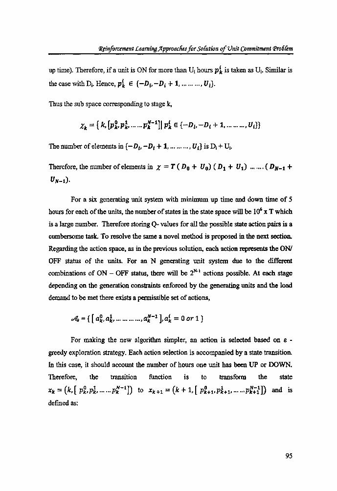
up time). Therefore, if a unit is ON for more than Vi hours pi is taken as V j• Similar is

the case with Dj. Hence, pL E {-Dj, - D i + 1, ......... , U I}.

Thus the sub space corresponding to stage le,

Therefore, the number of elements in Z = T (Do + Uo) (D1 + Ut) ....... (DN- 1 +

UN- t ).

For a six generating unit system with minimum up time and down time of 5

hours for each of the units, the number of states in the state space will be 1 (f x T which

is a large number. Therefore storing Q- values for all the possible state action pairs is a

cumbersome task. To resolve the same a novel method is proposed in the next section.

Regarding the action space, as in the previous solution. each action represents the ONI

OFF status of the units. For an N generating unit system due to the different

combinations of ON - OFF status, there will be 2N-I actions possible. At each stage

depending on the generation constraints enforced by the generating units and the load

demand to be met there exists a permissible set of actions,

.A .. = {[ a~,al, ............ ,a:-1 ],a~ = 0 or 1}

For making the new algorithm simpler, an action is selected based on e -

greedy exploration strategy. Each action selection is accompanied by a state transition.

In this case, it should account the number of hours one unit has been UP or OOWN.

Therefore, the transition function is to transform the state

X1c = (k, [ p~, p~, ...... p:-t]) to xk +1 = (k + 1, [ P~+lI P~+1' ...... p:;l]) and is

defmedas:

95

Cfiapter4

pL+l = Pt + 1, if Pt positive, a~ = 1 pt+l = -1, if Pt positive, a~ = 0

pt+! = Pk - 1, if Pt negtive, aL = 0

pL+l = + 1, if Pt negative, aL = 1

pt+l = Ut, if Pt > Ut

Pk+l = Di , if Pk < Di

(4.10)

Since each action corresponds to a particular unit combination of generating

units to be on-line, the cost of generation or reward will be the function g (X.b at" X1+J)

as given in equation( 4.5).

Q learning described previously is used for solution of this MOP. Q values of

each state - action pairs are to be stored to find the good action at a particular state. In

this Unit Commitment Problem, when the minimum up time and down time constraints

are takeh, the possible states come from a very large state space. Straight forward

method of storing the Q (XIo aJ values is using a look up table. But all the states in this

huge state space are not relevant. Therefore a novel method of storing Q values is

suggested.

Q values of only those states which are encountered at least once in the course

of learning are stored. Since the learning process allows sufficient large number of

iterations, this seems to be a valid direction. The states are represented by an index

number (ind _x,J, which is an integer and initialized at the first time of encountering

the state. For example the tuple, (5, (2,[-2,1,1,2])) denote the state (2, [-2,1,1,2]) with

an index number' 5'.

Similarly, the actions in the action space can also be represented by an integer,

which is the decimal equivalent of the binary string representing the status of the

different units. The index value of action 0011 is '3'. Using these indices for the state

and action strings, the Q values of the different state action pairs can be stored very

easily. Q (5,3) indicate the Q value corresponding to the state (2, [-2, 1, 1,2]). which

is having index value 5 and action [00 I 1].

96

CJ(pnjMcement Learning ;4pproacfies for Sofution of Vnit Commitment 'l'ro6fem

The possible number of states nstates is initialized depending on the number of

units N and the minimum down time and minimum up time of the units, since it

depends on number of combinations possible with N units as well as the given values

of minimum up time and down time. Since some of the states will not be visited at all,

the value of lIStates is initialized to 70010 of the total number states. The number of

actions 'naction' is initialized to 2N -1. Then the permissible action set corresponding

to each hour based on the load demand at that particular hour are identified. The

algorithm during the learning phase proceeds as follows.

At each hour k, the state Xl depending on the previous state and action is found

as explained previously. The state Xl is added to the set of states b if not already

present and frod the index of the state Xl. From the permissible action set, one of the

actions is chosen based on &-greedy method. Then the next state Xt+1 can be found

corresponding to stage k+ J. On taking action ak, the state of the system proceeds from

x .. to Xt+1 as given in (4.10). The reward, g (xj) aj) Xt+I) is given by equation (4.5).

The Q value corresponding to the particular hour Ok', action 'a .. ' (decimal

value of the binary string) and index no (ind_xk) is then updated using the equation:

Q7l+1(ind_Xk,ak) = Q71(ind...xk,ak) + a [g(xk,ak,Xt+1)

+ Y ,min Q71 (ind_xk+l' a') - Q" (Cnd...xt, ak)] a EcIlt+l

(4.11)

If the stage is the last one (le = 1), corresponding to the last hour to be

scheduled, there is no more succeeding stages and the updating equation reduces as,

Q71+1(ind_xk, ak) = Q7l{ind_xt, ak) + a [n(Xt, at, Xt+l) - Q" (Cnd...xt, at)]

(4.12)

At each episode of the learning phase, the algorithm passes through all the 'T'

stages. As the algorithm completes several iterations, the estimated Q values will reach

nearer to the optimum values and then the optimum schedule or allocation can be

easily retrieved for each stage k as, ak =: arg minakEcIlt{Q{ind_xk, at»)

The entire algorithm is illustrated as RL _ UCP3.

97

Cfiapter4

98

Algorithm for Unit Commitment using state indl!'Xing (RL_ UCP3)

Read Unit Data

Read the initial status of the units, Xo

Read the Loadforecastfor next T hours

Initialize 'nstates' (number of states) and 'nactions' (number of actions)

Initialize (f {ind_xh aJ =0, 0 < ind_xt<= nstates,O < al:<= nactions

Find the set of permissible actions corresponding to each hour k

Initialize E = 0.5 and a =0.1

For n=J to max iteration

Begin

End

Read the initial status of the units Xo

Add the state Xo to set Zo

For k=0 to T-J

Do

Find the feasible set of actions d4 corresponding to state Xt

considering up and down times.

Choose an action using So greedy strategy from

the feasible set of actions

Find the next state XHl

IfxHl is present in ZHI Get the index ind_xk+l

Else Add Xk+l in Zk+l and obtain index ind _ XHl

Calculate cost as g(Xh ah Xk+V

If (k /= T-J) Update Q value using equation (4.11)

Else Update Q value using equation (4. J 2)

ind_xt = ind_xH/.

End do

Update the value of &

Save Q values.

10nforcement £eaming Jlpproac/ies for So(utWn ofVnit Commitment Pro6fem

This algorithm can accommodate the minimum up time and down time

constraints easily, when the number of generating units is small. Up to 5 hours of

minimum up time and minimum down time the algorithm is found to work efficiently.

But when the minimum up time and minimum down time increase beyond 5 hours and

the number of generating units is beyond six, the number of states visited increases.

Then the number of Q values stored and updated becomes enormously larger. This

demands more computer memory. In order to solve this issue and make an efficient

solution, in the next section a state aggregation method is discussed which needs much

less computer memory than the above formulated algorithm.

4.10 Reinforcement Learning algorithm for UCP, through State

Aggregation (RL_UCP4)

While looking into the Unit Commitment Problem with minimum up time and

minimum down time constraints, the state space become very huge. The huge state

space is difficult to handle in a straight forward manner when the minimum up time I

minimum down time increases or the number of generating unit increases. Storing of Q

value corresponding to each state - action pair becomes computationally expensive.

Some method is to be thought of to reduce the number of Q values to be handled. In

the perspective of Unit Commitment problem one can group the different states having

the same characteristics so that the goodness of the different groups is stored instead of

goodness of the different states corresponding to an action. The grouping of states can

be done based on the number of hours a unit has been UP or DOWN.

(i) A machine which has been already UP for duration equal to or greater than the

minimum up time can be considered as to occupy a state 'can be shut down'.

(ii) A unit which is already UP but not have covered minimum up time can be

considered as to represent a state 'cannot be shut down'.

99

Cfiapter4

(iii) An already offline unit which has been DOWN for number of hours equal to or

more than its minimum down time can be represented as a state • can be

committed' .

(iv) A unit which has been DOWN but has not covered the minimum down time so

that cannot be committed in the next immediate slot of time can be represented

as a state 'cannot be committed'.

Thus, at any slot of time, each of the generating unit will be in any of the

above mentioned four representative states. If these four conditions are denoted as

decimal integers (0, 1, 2, 3), regardless of the UP time and DOWN time of a generating

unit, the state is represented by one of this integer value. By aggregating the numerous

states visited in the previous algorithm to a limited number of states, number of Q

values to be stored and updated in the look up table is greatly reduced.

With the decimal numbers 0,1,2,3 representing the aggregated states of a unit,

for an N generating unit system the state Xl is represented as a string of integers having

length N and with each integer having any of these four values. Then the state can be

represented as a number with base value 4. For an N generating unit problem, there

will be 4N -1 possible states, regardless of minimum up time and down time of the

different units. (In the previous algorithm RL_UCP3. the number of states increases

with increase in the minimum up time and / or down time). This reduction in the

number of states drastically reduces the size of look up table for storing the Q values.

Now an algorithm is formulated making use of state aggregation technique for

handling the up/ down constraints of the units.

The number of states, nstates is initialized to 4N -1 and the number of actions

naction to 2N_l for an N generating unit system. At any stage kofMDP, the state of the

system is represented as a string of integers as in the previous algorithm, integer value

representing the number of hours the unit has been up or down.

100

IJ{finforcement £earning }lpproacms for Sofuticn ofVnit Commitment Ch'o6fem

In order to store the Q values, the state Xl is mapped into set of aggregate

states. Each aggregate state,

ag...x/c = {(k, [ag-pZ, ag"p~, ... ... ag-p:-1 D, ag-p~ E { 0,1,2,3}.

From any state Xl an action is selected using one of the exploration strategies.

On selecting an action ah the status of the units will change as, Xk+1 = f(x", aJ given by

equation (4.10). From the above explained categorization of states, ag..,p1 can be

found corresponding to any Xk = (k, [p~, pl, ...... p~-l ]) as:

I·· d'>U '0 p" posItIve an Plc - b ag-p,,::: ;

I·· d' U i 1 Plc positive an Plc < t, ag..,plc = ;

p~ negative and p~ =:; D" ag-p~ = 2;

, . d' D '3 Plc negative an Plc> - "ag..,p" = .

The reward function for the state transition is found using the cost evaluations

of the different generating units using equation (4.5). For each of the states Xl and Xk+/.

the corresponding aggregate state representation is found as ag_xl and ag_Xk+/ . Each

action in the action space is represented as the decimal equivalent of the binary string.

At each state K, estimated Q value corresponding to the state - action pair (ag_x", aJ is

updated using the equation,

Qn+1(ag_x/c,a/c) = Qn(ag_x/c,a/c) + a [g(x/c,a/c,x/C+1)

+ Y ,min Qn (ag..x/C+lI a') - Qn (ag_x/c, a/c)] a E.Jtlc+l

(4.13)

During the last hour, omitting the term to account future pay -off Q value is

updated using the equation,

101

Cliapter4

Qn+1(ag_Xk. ak) = Qn(ag_XIe' ale) + a [g(x", a". XIe+l)

- Qn (ag_x". ale)]

(4.14)

After a number of iterations, learning converges and the optimum schedule or

allocation for each state Xl can be easily retrieved after rmding the corresponding

aggregate state as,

The entire algorithm using state aggregation method is given below:

102

Algorithm for Unit Commitment through state aggregation (RL _ UCP4)

Read Unit Data

Read the Load forecast for next T hours.

Initialize nstates (number of states) and nactions (number of actions)

Initialize (f [ag_xb aJ =0. V ag_xlo V at

Find the set of permissible actions corresponding to each hour k

Initialize the learning parameters

For n=J to max _ episode

Begin

Read the initial status of the units Xo

For k=0 to T-J

Do

Find aggregate state ag_ Xl corresponding to X.t

Find the foasible set of actions eIlt corresponding to state Xl

considering up and down times.

Choose an action using ~ greedy strategy from the foasible set

of actions

Contd ...

~info(cement Learnins jlpproaches for So(ution ofVnit Commitment ~6Cem

Find the next state Xk+l

End do

Find the corresponding aggregate state ag_xJ:+J ofxk+l

Calculate the reward g (Xl, ,ah Xk+J

If (k 1= T-l) Update Q value using equation (4. J 3)

Else Update Q value using equation (4.14)

Update the value of E:.

End

Save Q values.

The optimal schedule [aO. ai, ..... aT-l] is obtained using policy retrieval

steps similar to the algorithm given in section 4.8.

4.11 Performance Evaluation

Solution to Unit Commitment Problem has now been proposed by various

Reinforcement Learning approaches. Now, one can validate and test the efficacy of the

proposed methods by choosing standard test cases. The high level programming code

for the algorithms is written in C language in Linux environment. The execution times

correspond to Pentium IV, 2.9 GHz, 512 MB RAM personal computer.

In order to compare the e greedy and pursuit solutions (RL_UCPl and

RL _ UCP2) a four generating unit system and an eight generating unit system are

considered. The generation limits, incremental and start up cost of the units are

specified. Performance of the two algorithms is compared in terms of number of

iterations required in the learning phase and the computation time required for getting

the commitment schedule.

In order to validate and compare the last two algorithms (RL _ UCP3 and

RL_UCP4), four generating unit system with different minimum up time and down

time are considered. The schedule obtained is validated and the performance

comparison is made in terms of execution time of the entire algorithm, including the

learning and policy retrieval. In order to prove the scalability of the algorithms, an

103

Cliapter4

eight generating unit system with given minimum up time and down time limits is also

taken for case study.

For comparing with the recently developed stochastic strategies a ten

generating unit system with different minimum up time and down time limits are taken

for case study. The schedule obtained and the computation time is compared with two

hybrid methodologies: Simulated Annealing with Local Search (SA LS) and Lagrange

Relaxation with Genetic Algorithm (LRGA).

In order to apply the proposed Reinforcement Learning algorithms, first

suitable values of the learning parameters are to be selected Value of E balances the

rate of exploration and exploitation. For balancing exploration and exploitation, a value

of 0.5 is taken for the learning parameter e initially. In every (maxjteraionllO)

iterations, s is reduced by 0.04 so that in the final phases, s will be 0.1.

Discount parameter y accounts for the discount to be made in the present state

in order to account of future reinforcements and since in this problem, the cost of

future stages has the same implication as the cost of the current stage, value of y is

taken as 1. The step size ofleaming is given by the parameter a and it affects the rate

of modification of the estimate of Q value at each iteration step. By trial and error a is

taken as 0.1 in order to achieve sufficiently good convergence of the learning system.

The RL parameters used in the problem are also tabulated in Table 4.1.

Table 4.1- RL Parameters

E 0.5

a 0.1

y 1

Now the different sample systems and load profile are considered, for

evaluating the performance of the algorithms.

104

CJ?Pnforcement LeaminoJlpproadies for So(ution ofVnit Commitment (}To6fem

Case I-A/our generating unit system

Consider a simple power system with four thermal units (Wood and

WoUenberg [2002]). For testing the efficacy of the first two algorithms and to compare

them, minimum up and down times are neglected. Load proflle for duration of 8 hours

is considered and is given in Table 4.2

Table 4.2 - Load profde for eight hours

Hour 0 1 2 3 4 5 6 7

Load(MW) 450 530 600 540 400 280 290 500

The cost characteristics of the different units are taken to follow a linear

incremental cost curve. That is, cost of generating a power Pt by the ,.u. unit is given as,

C, (PJ =NLj + lCt • Pp

where NLI represents the No Load cost of t unit and lCj is the Incremental cost of the

same unit. The values P",iII and P 1fIIJX represent the minimum and maximum values of

power generation possible for each of the units. The different unit characteristics and

the generation limits are given in Table 4.3.

Table 4.3 - Generating Unit Characteristics

Unit Pmin(MW) Pmax(MW) Incremental No Load Startup cost Cost Cost Rs. Rs. Rs.

1 75 300 17.46 684.74 1100

2 60 250 18 585.62 400

3 25 80 20.88 213 350

4 20 60 23.8 252 0.02

105

Cliapter4

When the learning is carried out using the flrst two algorithms, learning is flrst

carried to fmd the maximum number of iterations required for the learning procedure.

In the learning procedure, 100 consecutive iterations are examined for

modiflcation in the estimated Q values. If the change is negligibly small in all these

100 iterations, the estimated Q values are regarded as optimum corresponding to a

particular state - action pair. The iteration number thus obtained is approximated to

nearest multiple of 100 is taken as 'maximum iteration (maxjteration), and used in

next trials. Different successive executions of the algorithm with max_iteration

provided with almost the same results with tolerable variation.

RL _ UCP 1 indicated the convergence after 5000 iterations. While using

RL_UCP2 the optimum is reached in 2000 iterations. The schedule obtained is given in

Table 4.4 which is same as given in Wood and Wollenberg [2(02).

Table 4.4 - Commitment sthedule obtained

Hour 0 1 2 3 4 5 6 7

State 0011 0011 1011 0011 0011 0001 0001 0011

The computation time taken by RL_VCP 1 was 15.62 sec while that taken by

RL_VCP2 was only 9.45sec. From this, it can be inferred that, the pursuit method

is faster.

Case IJ- Eight generating unit system

Now an eight generating unit system is considered and a load profIle of 24

hours is taken into account in order to prove the scalability of the algorithms. The load

proflle is given in Table 4.5

106

fJ(sinforcement Leami1t{jJlpproacfies for So(ution ofVnit Commitment (]>ro6fem

Table 4.5 - Load profile for 24 hours

Hour 0 1 2 3 4 5 6 7

Load(MW) 450 530 600 540 400 280 290 500

Hour 8 9 10 11 12 13 14 15

Load(MW) 450 530 600 540 400 280 290 500

Hour 16 17 18 19 20 21 22 23

Load(MW) 450 530 600 540 400 280 290 500

The cost characteristics are assumed to be linear as in previous case. The generation

limit and the cost characteristics are given in Table 4.6

Table 4.6 - Gen. Unit characteristics for Eight generator system

Incremental No. Load Startup Unit Pmin Pmax Cost Cost Cost

(MW) JMWl Rs. Rs. Rs. 1 75 300 17.46 684.74 1100

2 75 300 17.46 684.74 1100

3 60 250 18 585.62 400

4 60 250 18 585.62 400

5 25 80 20.88 213 350

6 25 80 20.88 213 350

7 20 60 23.8 252 0.02

8 20 60 23.8 252 0.02 . .

The optimal cost obtained for 24 hour penod 1S Rs. 219,5961- and the solution

obtained is given in Table 4.7. The status of the different units is expressed by the

decimal equivalent of the binary string. For example during the first hour, the

scheduled status is '3', which indicate 0000 001 L

107

ClUJpter4

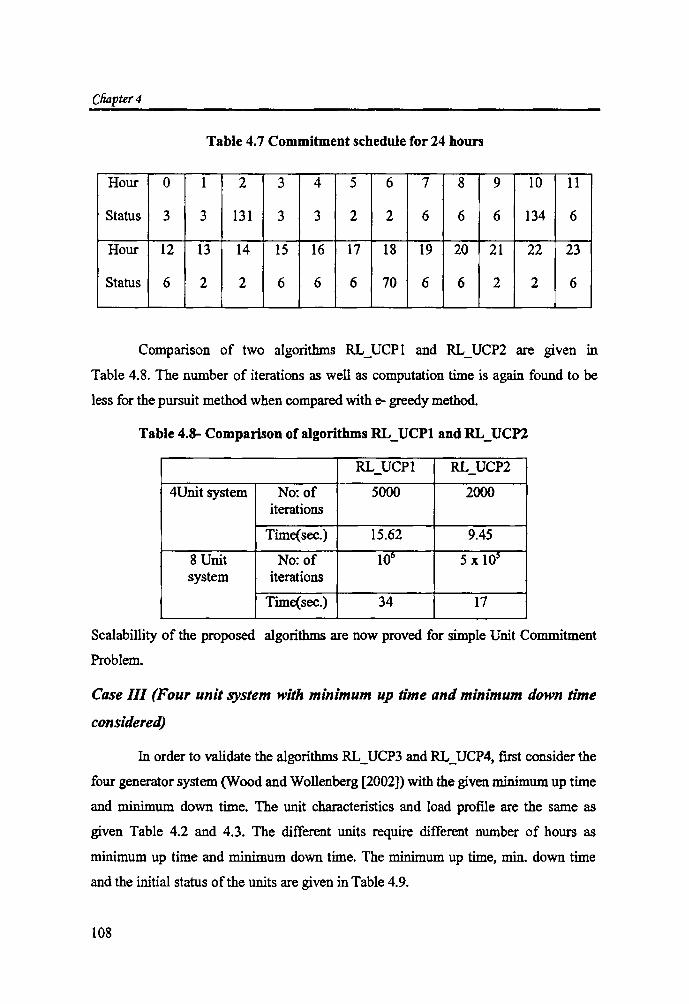
Table 4.7 Commitment schedule for 24 hours

Hour 0 1 2 3 4 5 6 7 8 9 10 11

Status 3 3 131 3 3 2 2 6 6 6 134 6

Hour 12 13 14 15 16 17 18 19 20 21 22 23

Status 6 2 2 6 6 6 70 6 6 2 2 6

Comparison of two algorithms RL _ UCP 1 and RL _ UCP2 are given in

Table 4.8. The number of iterations as well as computation time is again found to be

less for the pursuit method when compared with e- greedy method.

Table 4.8- Comparison oCalgorithms RL_UCPl and RL_UCPl

RL_UCPl RL_UCP2

4Unit system No: of 5000 2000 iterations

Time(sec.) 15.62 9.45

8 Unit No: of 106 5 x IO~ system iterations

Time(sec.) 34 17

Scalabillity of the proposed algorithms are now proved for simple Unit Commitment

Problem.

Case III (Four unit system with minimum up time and minimum down time

considered)

In order to validate the algorithms RL_ UCP3 and RL_ UCP4, first consider the

four generator system (Wood and Wollenberg [2002]) with the given minimum up time

and minimum down time. The unit characteristics and load profile are the same as

given Table 4.2 and 4.3. The different units require different number of hours as

minimum up time and minimum down time. The minimum up time, min. down time

and the initial status of the units are given in Table 4.9.

108

~forcement Learning )lpproacfzes for So(utWn ofVnit Commitment 1Pro6fem

Table 4.9 - Minimum up time and minimum down time, initial status

Min. Min.Down

Unit Up ime(Hr.) time(Hr.) Initial Status

1 4 2 -2

2 5 3 1

3 5 4 -4

4 1 1 -1

The initial status -1 indicate that the particular unit has been DOWN for 1 hour

and the initial status 1 represent that the unit has been UP for 1 hour.

The learning of the system is carried out using RL _ VCP3 and RL_ UCP4. A

number of states are visited and after 10' iterations, the Q values approach optimum.

RL _ VCP3 enumerates and stores all the visited states. The goodness of each state

action pair is stored as Q value. On employing state aggregation in RL_UCP4, the

number of entries in the stored look up table is reduced prominently. This is reflected

by the lesser computation time. The optimum schedule obtained is tabulated in

Table 4.10 which is consistent with that given through Dynamic Programming (Wood

and Wollenberg [2002])

Table 4.10 - Optimum schedule obtained

Hour 1 2 3 4 5 6 7 8

Status 0110 0110 0111 0110 0110 OllO 0110 0110

In RL _ VCP3, since the number of states and hence the number of Q values

manipulated are more, the execution time is more. In case of RL _ VCP4, the number of

states is drastically reduced due to the aggregation of states and hence the schedule is

obtained in much lesser time. Time of execution of the algorithms RL _ VCP3 and

RL_VCP4 are tabulated for comparison in Table 4.11

109

Cfiapter4

Table 4.11 -Comparison of RL_ UCPJ and RL_ UCP4

Execution Algorithm Time (Sec.)

RL_UCP3 9.68

RL UCP4 3.89

From the comparison of execution time, it can be seen that state aggregation

has improved the performance very much.

Case IV-Ten generating unit system

In order to prove the flexibility of RL_UCP4 and to compare with other

methods, next a ten generating unit with different initial status given is considered

(Cheng et al. [2000J).

In this case minimum up time and minimum down time are also different for

different units. Minimum up time of certain units is 8 hours, which is difficult to be

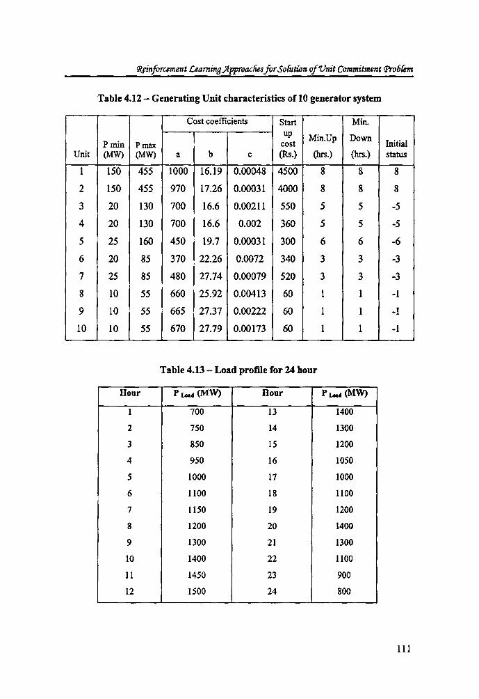
handled by RL_UCP3. The cost functions are given in quadratic cost form, C(P) =

a + bP + cp2, where a,b and c are cost coefficients and P the power

generated. The values of the cost coefficients a, b and c for the different generating

units are given in Table 4.12. For a load profile of eight hours given in Table 4.13, the

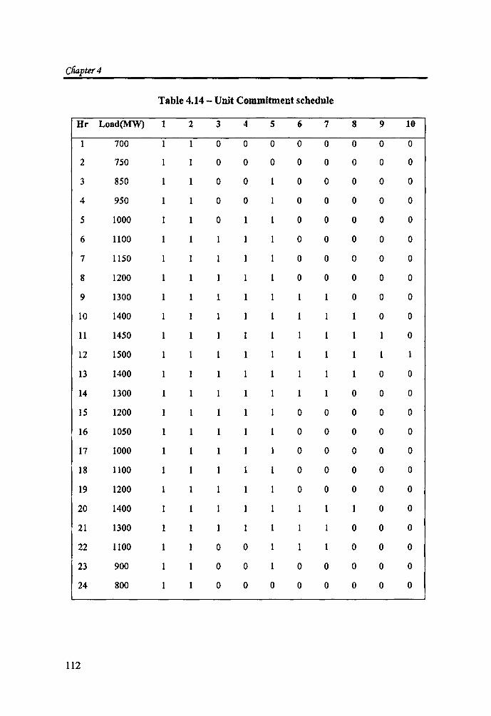
algorithm gave an optimum result in 2 x 10$ iterations. The obtained commitment

schedule is given in Table 4.14

110

'J?iinforcement £eamino .JlpproacfieJ for So(ution ofVnit Commitment Pro6Cem

Table 4.12 - Generating Unit characteristics of 10 generator system

Cost coefficients Start Min. up Min.Up Down

Pmin Pmax cost Initial Unit (MW) (MW) a b c (Rs.) (hrs.) (hrs.) status

1 150 455 1000 16.19 0.00048 4500 8 8 8

2 150 455 970 17.26 0.00031 4000 8 8 8

3 20 130 700 16.6 0.00211 550 5 5 -5

4 20 130 700 16.6 0.002 360 5 5 -5

5 25 160 450 19.7 0.00031 300 6 6 -6

6 20 85 370 22.26 0.0072 340 3 3 -3

7 25 85 480 27.74 0.00079 520 3 3 -3

8 10 55 660 25.92 0.00413 60 1 1 -1

9 10 55 665 27.37 0.00222 60 1 1 -1

10 10 55 670 27.79 0.00173 60 1 1 -1

Table 4.13 - Load profile for 24 hour

Hour PLead (MW) Hour PLead (MW)

1 700 13 1400

2 750 14 1300

3 850 15 1200

4 950 16 1050

5 1000 17 1000

6 1100 18 1100

7 1150 19 1200

8 1200 20 1400

9 1300 21 1300

10 1400 22 1100

11 1450 23 900

12 1500 24 800

111

Cfiapter4

Table 4.14 - Unit Commitment schedule

Hr Load(MW) 1 2 3 4 S 6 7 8 9 10

700 0 0 0 0 0 0 0 0

2 750 0 0 0 0 0 0 0 0

3 850 0 0 0 0 0 0 0

4 950 1 0 0 0 0 0 0 0

5 1000 1 0 1 0 0 0 0 0

6 1100 0 0 0 0 0

7 1150 0 0 0 0 0

8 1200 0 0 0 0 0

9 1300 1 1 1 0 0 0

10 1400 1 0 0

11 1450 0

12 1500 1 1 1

13 1400 1 1 0 0

14 1300 1 1 1 0 0 0

15 1200 0 0 0 0 0

16 1050 1 1 0 0 0 0 0

17 1000 1 1 1 0 0 0 0 0

18 HOO 1 1 0 0 0 0 0

19 1200 0 0 0 0 0

20 1400 0 0

21 1300 1 1 1 0 0 0

22 1100 1 0 0 1 0 0 0

23 900 0 0 0 0 0 0 0

24 800 1 0 0 0 0 0 0 0 0

112

rf<Iinforcement Ltarnina ~pproaclies for Solution ofVnit Commitment (]lro6km

By executing RL_ UCP4 for the above characteristics, the commitment

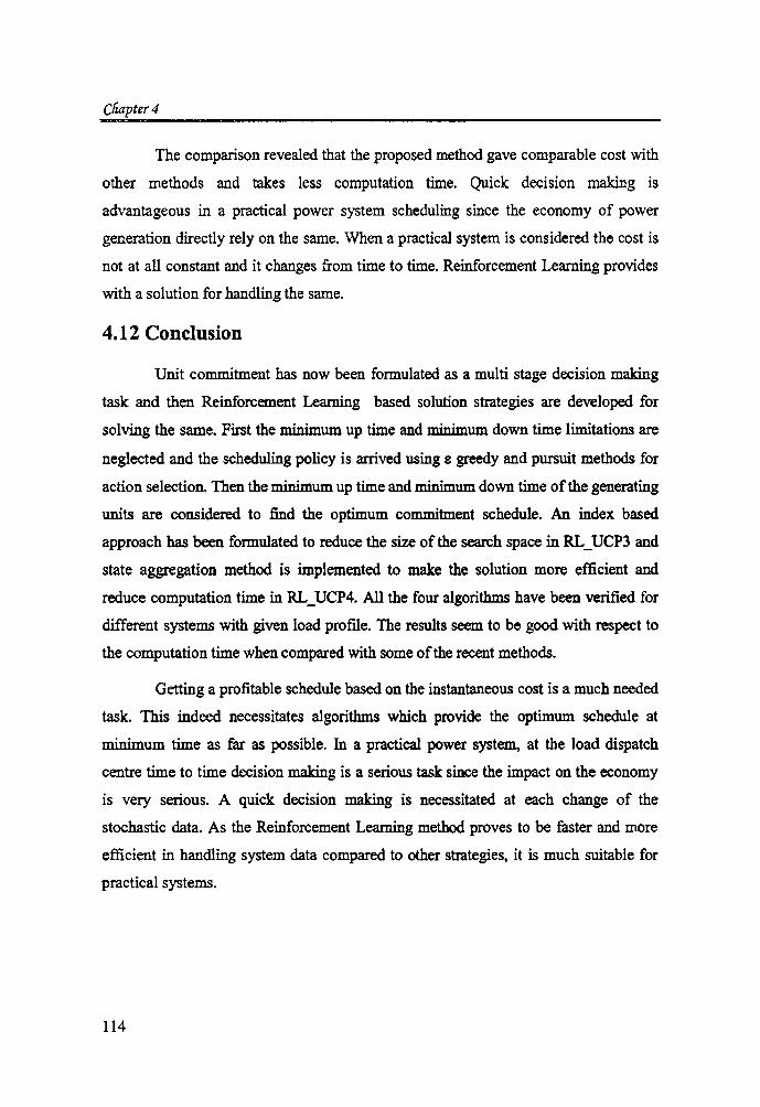
schedule is obtained in 268 sec. The obtained schedule is given in Table 4.14. The cost

obtained and the computation time are compared with that obtained through hybrid

methods using Lagrange Relaxation and Genetic Algortihm (LRGA) proposed by

Cheng et al. [2000] and Simulated Annealing and Local search (SA LS) suggested by

Purushothama and Lawrence Jenkins.[2003]. Comparison of the cost and time are

given 4.15.

Table 4.15 - Comparison of cost and time

Execution

Algorithm Cost(Rs.) Time(sec.)

LRGA 564800 518

SA LS 535258 393

RL_UCP4 545280 268

A graphical representation of Table 4.15 is given in 4.1

600

500

:f400 .Ji 0;­E300 F U ~200 w

100

o +--

518 sec

10 gen system

. lRGA

. SALS

• Rl_UCP4

Fig 4.1 Comparison of execution time (,~.) of RL approacb

witb other metbod,

113

Cliapter4

The comparison revealed that the proposed method gave comparable cost with

other methods and takes less computation time. Quick decision making is

advantageous in a practical power system scheduling since the economy of power

generation directly rely on the same. When a practical system is considered the cost is

not at all constant and it changes from time to time. Reinforcement Learning provides

with a solution for handling the same.

4.12 Conclusion

Unit commitment has now been formulated as a multi stage decision making

task and then Reinforcement Learning based solution strategies are developed for

solving the same. First the minimum up time and minimum down time limitations are

neglected and the scheduling policy is arrived using £ greedy and pursuit methods for

action selection. Then the minimum up time and minimum down time of the generating

units are considered to find the optimum commitment schedule. An index based

approach has been formulated to reduce the size of the search space in RL_VCP3 and

state aggregation method is implemented to make the solution more efficient and

reduce computation time in RL_VCP4. All the four algorithms have been verified for

different systems with given load profile. The results seem to be good with respect to

the computation time when compared with some of the recent methods.

Getting a profitable schedule based on the instantaneous cost is a much needed

task. This indeed necessitates algorithms which provide the optimum schedule at

minimum time as far as possible. In a practical power system, at the load dispatch

centre time to time decision making is a serious task since the impact on the economy

is very serious. A quick decision making is necessitated at each change of the

stochastic data. As the Reinforcement Learning method proves to be faster and more

efficient in handling system data compared to other strategies, it is much suitable for

practical systems.

114