Multi-Agent Reinforcement Learning Approaches for ...
173
Multi-Agent Reinforcement Learning Approaches for Distributed Job-Shop Scheduling Problems Vom Fachbereich Mathematik/Informatik der Universit¨ at Osnabr¨ uck zur Verleihung des akademischen Grades Doktor der Naturwissenschaften (Dr. rer. nat.) genehmigte Dissertation von Diplom-Informatiker Thomas Gabel Berichterstatter: Prof. Dr. Martin Riedmiller, Universit¨ at Osnabr¨ uck, Deutschland Prof. Dr. H´ ector Mu˜ noz-Avila, Lehigh University, USA Pr¨ ufungskommision: Prof. Dr. Martin Riedmiller Prof. Dr. Volker Sperschneider Prof. Dr. Werner Brockmann Dr. Andreas N¨ uchter Tag der wissenschaftlichen Aussprache: 26.06.2009
Transcript of Multi-Agent Reinforcement Learning Approaches for ...
Multi-Agent Reinforcement LearningApproaches for Distributed
Job-Shop Scheduling Problems
Vom Fachbereich Mathematik/Informatik
der Universitat Osnabruck
zur Verleihung des akademischen Grades
Doktor der Naturwissenschaften (Dr. rer. nat.)
genehmigte Dissertation
von
Diplom-Informatiker Thomas Gabel
Berichterstatter:Prof. Dr. Martin Riedmiller, Universitat Osnabruck, Deutschland
Prof. Dr. Hector Munoz-Avila, Lehigh University, USA
Prufungskommision:Prof. Dr. Martin Riedmiller
Prof. Dr. Volker SperschneiderProf. Dr. Werner Brockmann
Dr. Andreas Nuchter
Tag der wissenschaftlichen Aussprache: 26.06.2009

Acknowledgements
This work was developed during my time as a member of the Neu-roinformatics Group at the University of Osnabruck, Germany.A major portion of the research presented in this document wasconducted within the scope of the project “Learning Algorithmsfor Cooperative Multi-Agent Systems” which was funded by theGerman Research Foundation (DFG). I therefore would first liketo thank the DFG for their financial support.Many people have influenced my work during the previous yearsand it is nearly impossible to list all of them. However, I wouldlike to mention a few persons to whom I am particularly indebted.First of all, I would like to thank my supervisor, Prof. Dr. MartinRiedmiller, for his commitment to serve as my doctoral advisorand for his continued support in scientific and occupational ques-tions. Moreover, he has nurtured the development of inspiring andcomfortable working conditions in his research group that, in myopinion, were beyond compare.Furthermore, I would like to thank Prof. Dr. Hector Munoz-Avila for his great job as a co-referee of this thesis, as well asProf. Dr. Volker Sperschneider, Prof. Dr. Werner Brockmann, andDr. Andreas Nuchter for serving on the board of disputation ex-aminers.I would also like to thank all my former students as well as my col-leagues, Roland Hafner, Sascha Lange, Martin Lauer, and StephanTimmer, for a harmonious working atmosphere, for interesting andencouraging discussions, as well as exciting conference travels. Iam also greatly indebted to Thorsten Kundoch for his technicaland IT support as well as to Anna Rushing-Jungeilges for heradministrative support and her proofreading of nearly all of mypublications and parts of this thesis.I owe special thanks to Susanne Linster for proofreading the finalversion of this thesis. Last but not least, I owe many thanks to myparents and family for supporting me in countless ways throughoutthe years.
Osnabruck, July 2009

Abstract
Decentralized decision-making has become an active research topic in artificial intelligence. In adistributed system, a number of individually acting agents coexist. If they strive to accomplisha common goal, i.e. if the multi-agent system is a cooperative one, then the establishment ofcoordinated cooperation between the agents is of utmost importance. With this in mind, ourfocus is on multi-agent reinforcement learning methods which allow for automatically acquiringcooperative policies based solely on a specification of the desired joint behavior of the wholesystem.
Research in distributed systems has pointed out that the decentralization of the control ofthe system and of the observation of the system among independent agents has a significantimpact on the complexity of solving a given problem. Therefore, we address the intricacy oflearning and acting in multi-agent systems by the following complementary approaches.
Many practical problems exhibit some structure whose exploitation may ease the task offinding solutions. For this reason, we are going to identify a subclass of general decentralizeddecision-making problems that features regularities in the way the agents interact with oneanother. We will show that the complexity of optimally solving a problem instance from thisclass is provably lower than solving a general one.
Even though a lower complexity class may be entered by sticking to certain subclasses of ageneral multi-agent problem, the computational complexity may be still so high that optimallysolving it is infeasible. This holds, in particular, when intending to tackle problems of largersize that are of relevance for practical problems. Given these facts, our goal will be not todevelop optimal solution algorithms that are applicable to small problems only, but to look fortechniques capable of quickly obtaining approximate solutions in the vicinity of the optimum.To this end, we will develop and utilize various model-free reinforcement learning approaches.In contrast to offline planning algorithms which aim at finding optimal solutions in a model-based manner, reinforcement learning allows for employing independently learning agents and,hence, for a full decentralization of the problem.
As a matter of fact, many large-scale applications are well-suited to be formulated in termsof spatially or functionally distributed entities. Thus, multi-agent approaches are of highrelevance to various real-world problems. Job-shop scheduling is one such application stemmingfrom the field of factory optimization and manufacturing control. It is our particular goal tointerpret job-shop scheduling problems as distributed sequential decision-making problems,to employ the multi-agent reinforcement learning algorithms we will propose for solving suchproblems, and, moreover, to evaluate the performance of our learning approaches in the scopeof various established scheduling benchmark problems.

Contents
1 Introduction 1
1.1 Motivation . . . . . . . . . . . . . . . . . . . . . . . . . . . . . . . . . . . . . . 1
1.2 Objectives . . . . . . . . . . . . . . . . . . . . . . . . . . . . . . . . . . . . . . . 4
1.3 Outline . . . . . . . . . . . . . . . . . . . . . . . . . . . . . . . . . . . . . . . . 5
2 Single- and Multi-Agent Reinforcement Learning 7
2.1 The Reinforcement Learning Framework . . . . . . . . . . . . . . . . . . . . . . 7
2.1.1 Markov Decision Processes . . . . . . . . . . . . . . . . . . . . . . . . . 8
2.1.2 Learning Optimal Behavior . . . . . . . . . . . . . . . . . . . . . . . . . 9
2.1.3 On Actors and Critics . . . . . . . . . . . . . . . . . . . . . . . . . . . . 10
2.1.4 Policy Search-Based Reinforcement Learning . . . . . . . . . . . . . . . 10
2.1.5 Value Function-Based Reinforcement Learning . . . . . . . . . . . . . . 11
2.2 From One to Many Agents . . . . . . . . . . . . . . . . . . . . . . . . . . . . . 13
2.2.1 Cooperative and Non-Cooperative Multi-Agent Systems . . . . . . . . . 14
2.2.2 Application Fields of Learning Multi-Agent Systems . . . . . . . . . . . 14
2.3 Cooperative Multi-Agent Systems with Partial Observability . . . . . . . . . . 15
2.3.1 The Multi-Agent Markov Decision Process Model . . . . . . . . . . . . . 15
2.3.2 Partially Observable Markov Decision Processes . . . . . . . . . . . . . 17
2.3.3 The Framework of Decentralized Markov Decision Processes . . . . . . . 17
2.3.4 The Price of Decentralization . . . . . . . . . . . . . . . . . . . . . . . . 19
2.4 Decentralized Markov Decision Processes with Changing Action Sets . . . . . . 21
2.4.1 On Transition Dependencies . . . . . . . . . . . . . . . . . . . . . . . . . 21
2.4.2 Variable Action Sets and Partially Ordered Transition Dependencies . . 22
2.4.3 Implications on Complexity . . . . . . . . . . . . . . . . . . . . . . . . . 24
2.4.4 Example Applications . . . . . . . . . . . . . . . . . . . . . . . . . . . . 26
2.5 Related Work on Learning in Cooperative Multi-Agent Systems . . . . . . . . . 27
2.5.1 Alternative Frameworks for Distributed Control . . . . . . . . . . . . . 27
2.5.2 Optimal Solution Algorithms . . . . . . . . . . . . . . . . . . . . . . . . 27
2.5.3 Subclasses with Reduced Problem Complexity . . . . . . . . . . . . . . 28
2.5.4 Search for Approximate Solutions . . . . . . . . . . . . . . . . . . . . . . 28
i
Contents
3 Distributed Scheduling Problems 31
3.1 Foundations . . . . . . . . . . . . . . . . . . . . . . . . . . . . . . . . . . . . . . 32
3.1.1 The Classical Job-Shop Scheduling Problem . . . . . . . . . . . . . . . . 32
3.1.2 The Disjunctive Graph Model . . . . . . . . . . . . . . . . . . . . . . . . 34
3.1.3 Classical Benchmark Problems . . . . . . . . . . . . . . . . . . . . . . . 35
3.2 Multi-Agent Job-Shop Scheduling . . . . . . . . . . . . . . . . . . . . . . . . . . 36
3.2.1 Discussion of Distributed Scheduling . . . . . . . . . . . . . . . . . . . . 36
3.2.2 Job-Shop Scheduling as Decentralized Markov Decision Process . . . . . 37
3.3 Related Work on Solving Job-Shop Scheduling Problems . . . . . . . . . . . . . 40
3.3.1 Optimal and Near-Optimal Solution Algorithms . . . . . . . . . . . . . 40
3.3.2 Dispatching Priority Rules . . . . . . . . . . . . . . . . . . . . . . . . . 41
3.3.3 Artificial Intelligence-Based Approaches . . . . . . . . . . . . . . . . . . 42
4 Policy Search-Based Solution Approaches 45
4.1 Foundations . . . . . . . . . . . . . . . . . . . . . . . . . . . . . . . . . . . . . . 45
4.1.1 Policy Performance . . . . . . . . . . . . . . . . . . . . . . . . . . . . . . 46
4.1.2 Multi-Agent Policy Search Reinforcement Learning . . . . . . . . . . . . 47
4.2 Joint Equilibrium Policy Search . . . . . . . . . . . . . . . . . . . . . . . . . . . 48
4.2.1 Learning Joint Policies . . . . . . . . . . . . . . . . . . . . . . . . . . . . 49
4.2.2 Global Action Parameterization . . . . . . . . . . . . . . . . . . . . . . . 52
4.2.3 Theoretical Properties . . . . . . . . . . . . . . . . . . . . . . . . . . . . 53
4.2.4 Discussion . . . . . . . . . . . . . . . . . . . . . . . . . . . . . . . . . . . 55
4.2.5 Empirical Evaluation . . . . . . . . . . . . . . . . . . . . . . . . . . . . . 56
4.3 Gradient-Descent Policy Search . . . . . . . . . . . . . . . . . . . . . . . . . . . 61
4.3.1 Gradient-Descent Policy Learning . . . . . . . . . . . . . . . . . . . . . 62
4.3.2 Independent Agents and Decentralized Policy Gradient . . . . . . . . . 65
4.3.3 Policy Gradient under Changing Action Sets . . . . . . . . . . . . . . . 67
4.3.4 Discussion . . . . . . . . . . . . . . . . . . . . . . . . . . . . . . . . . . . 70
4.3.5 Empirical Evaluation . . . . . . . . . . . . . . . . . . . . . . . . . . . . . 72
4.4 Discussion . . . . . . . . . . . . . . . . . . . . . . . . . . . . . . . . . . . . . . . 80
4.4.1 Related Work . . . . . . . . . . . . . . . . . . . . . . . . . . . . . . . . . 80
4.4.2 Advantages and Limitations of JEPS and GDPS . . . . . . . . . . . . . 81
5 Value Function-Based Solution Approaches 85
5.1 Foundations . . . . . . . . . . . . . . . . . . . . . . . . . . . . . . . . . . . . . . 85
5.1.1 The Issue of Generalization . . . . . . . . . . . . . . . . . . . . . . . . . 85
5.1.2 Batch-Mode Reinforcement Learning . . . . . . . . . . . . . . . . . . . . 87
5.2 Distributed and Approximated Value Functions . . . . . . . . . . . . . . . . . . 90
ii
Contents
5.2.1 Independent Value Function Learners . . . . . . . . . . . . . . . . . . . 90
5.2.2 Neural Fitted Q Iteration . . . . . . . . . . . . . . . . . . . . . . . . . . 91
5.2.3 Heuristic NFQ Enhancements . . . . . . . . . . . . . . . . . . . . . . . . 93
5.3 Fitted Q Iteration with Neural Networks and Optimistic Assumption . . . . . . 96
5.3.1 Optimistic Q Learning . . . . . . . . . . . . . . . . . . . . . . . . . . . . 96
5.3.2 Optimism Under Partial State Observability . . . . . . . . . . . . . . . 98
5.3.3 Batch-Mode Learning of Distributed Q Values . . . . . . . . . . . . . . 100
5.4 Empirical Evaluation . . . . . . . . . . . . . . . . . . . . . . . . . . . . . . . . . 103
5.4.1 Experimental Set-Up . . . . . . . . . . . . . . . . . . . . . . . . . . . . . 103
5.4.2 Example Benchmarks . . . . . . . . . . . . . . . . . . . . . . . . . . . . 107
5.4.3 Benchmark Suites . . . . . . . . . . . . . . . . . . . . . . . . . . . . . . 112
5.4.4 Generalization Capabilities . . . . . . . . . . . . . . . . . . . . . . . . . 114
5.5 Discussion . . . . . . . . . . . . . . . . . . . . . . . . . . . . . . . . . . . . . . . 117
5.5.1 Related Work . . . . . . . . . . . . . . . . . . . . . . . . . . . . . . . . . 118
5.5.2 Advantages and Limitations of OA-NFQ . . . . . . . . . . . . . . . . . . 120
6 Communicating Agents and Optimal Schedules 123
6.1 Foundations . . . . . . . . . . . . . . . . . . . . . . . . . . . . . . . . . . . . . . 123
6.1.1 Reactive Policies and Their Limitations . . . . . . . . . . . . . . . . . . 123
6.1.2 Interaction Histories . . . . . . . . . . . . . . . . . . . . . . . . . . . . . 124
6.2 Resolving Transition Dependencies . . . . . . . . . . . . . . . . . . . . . . . . . 125
6.2.1 Interaction History Encodings . . . . . . . . . . . . . . . . . . . . . . . . 125
6.2.2 Communication-Based Awareness of Inter-Agent Dependencies . . . . . 128
6.3 Empirical Evaluation . . . . . . . . . . . . . . . . . . . . . . . . . . . . . . . . . 131
6.3.1 Example Benchmark . . . . . . . . . . . . . . . . . . . . . . . . . . . . . 131
6.3.2 Benchmark Suites . . . . . . . . . . . . . . . . . . . . . . . . . . . . . . 133
6.4 Discussion . . . . . . . . . . . . . . . . . . . . . . . . . . . . . . . . . . . . . . . 137
7 Conclusion 139
7.1 Summary . . . . . . . . . . . . . . . . . . . . . . . . . . . . . . . . . . . . . . . 139
7.2 Outlook . . . . . . . . . . . . . . . . . . . . . . . . . . . . . . . . . . . . . . . . 141
iii

Contents
iv
List of Figures
1.1 The Big Picture: Overview of the Thesis . . . . . . . . . . . . . . . . . . . . . . 5
2.1 Schematic View on Reinforcement Learning . . . . . . . . . . . . . . . . . . . . 8
2.2 The Actor-Critic Architecture . . . . . . . . . . . . . . . . . . . . . . . . . . . . 10
2.3 Modelling Frameworks for Learning in Single- and Multi-Agents Systems . . . 16
2.4 DEC-MDPs with Changing Action Sets: Local State of Agent i . . . . . . . . . 22
2.5 Exemplary Dependency Functions . . . . . . . . . . . . . . . . . . . . . . . . . 23
2.6 Exemplary Dependency Graphs . . . . . . . . . . . . . . . . . . . . . . . . . . . 24
2.7 Interaction History and Encoding Function . . . . . . . . . . . . . . . . . . . . 25
3.1 Example of a Classical Job-Shop Scheduling Problem . . . . . . . . . . . . . . . 33
3.2 Classes of Schedules . . . . . . . . . . . . . . . . . . . . . . . . . . . . . . . . . 33
3.3 Optimal Schedule for the Scheduling Problem FT6 . . . . . . . . . . . . . . . . 34
3.4 The Disjunctive Graph Model . . . . . . . . . . . . . . . . . . . . . . . . . . . . 36
4.1 Joint Equilibrium Policy Search with Local Policy Parameterization . . . . . . 50
4.2 Joint Equilibrium Policy Search with Global Policy Parameterization . . . . . . 52
4.3 Learning Performance of Joint Equilibrium Policy Search for the FT6 Benchmark 58
4.4 Policy Development within a Single Agent Using JEPSG . . . . . . . . . . . . . 59
4.5 Learning Progress for JEPS and JEPSG on 10x10 Problems . . . . . . . . . . . 60
4.6 Visualization of Possibilities of Convergence and Optimality of GDPS . . . . . 71
4.7 Probabilistic Disjunctive Graph . . . . . . . . . . . . . . . . . . . . . . . . . . . 74
4.8 Makespan Distribution for a Random Dispatcher on the FT6 Problem . . . . . 74
4.9 Learning Performance of Gradient Descent Policy Search for the FT6 Benchmark 76
4.10 Gradient Descent Policy Search Learning Performance from a Single Agent’s
Point of View . . . . . . . . . . . . . . . . . . . . . . . . . . . . . . . . . . . . . 77
4.11 Gradient-Descent Policy Search Applied to a Selection of 10x10 Problems . . . 79
5.1 The Batch-Mode Reinforcement Learning Framework . . . . . . . . . . . . . . . 89
5.2 System Architecture for Value Function-Based Reinforcement Learning . . . . . 91
5.3 Learning with NFQ and OA-NFQ for the FT6 Benchmark . . . . . . . . . . . . 109
5.4 Training Data Utilization with NFQ and OA-NFQ for the FT6 Benchmark . . 110
v

List of Figures
5.5 Learning Process for the Notorious FT10 Problem . . . . . . . . . . . . . . . . 112
5.6 Learning Progress of OA-NFQ for 10x10 Job-Shop Scheduling Problems . . . . 113
5.7 Benchmark Results for OA-NFQ . . . . . . . . . . . . . . . . . . . . . . . . . . 114
5.8 Generalization Capabilities of OA-NFQ-Trained Agents . . . . . . . . . . . . . 116
6.1 Communication-Based Awareness of Inter-Agent Dependencies . . . . . . . . . 129
6.2 Learning Curves Using Encoding-Based and Communicating Agents for the FT6
Benchmark . . . . . . . . . . . . . . . . . . . . . . . . . . . . . . . . . . . . . . 133
6.3 Communication-Based GDPS Learning Progress for the FT10 Problem . . . . . 136
vi
1 Introduction
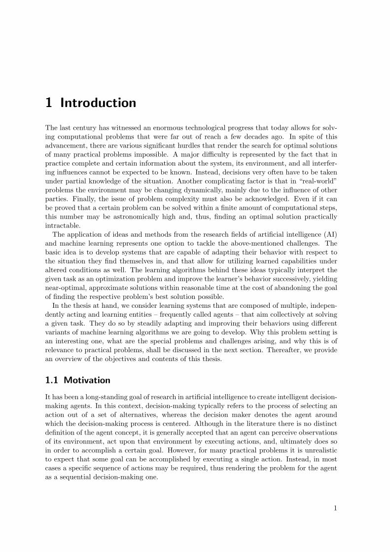
The last century has witnessed an enormous technological progress that today allows for solv-ing computational problems that were far out of reach a few decades ago. In spite of thisadvancement, there are various significant hurdles that render the search for optimal solutionsof many practical problems impossible. A major difficulty is represented by the fact that inpractice complete and certain information about the system, its environment, and all interfer-ing influences cannot be expected to be known. Instead, decisions very often have to be takenunder partial knowledge of the situation. Another complicating factor is that in “real-world”problems the environment may be changing dynamically, mainly due to the influence of otherparties. Finally, the issue of problem complexity must also be acknowledged. Even if it canbe proved that a certain problem can be solved within a finite amount of computational steps,this number may be astronomically high and, thus, finding an optimal solution practicallyintractable.
The application of ideas and methods from the research fields of artificial intelligence (AI)and machine learning represents one option to tackle the above-mentioned challenges. Thebasic idea is to develop systems that are capable of adapting their behavior with respect tothe situation they find themselves in, and that allow for utilizing learned capabilities underaltered conditions as well. The learning algorithms behind these ideas typically interpret thegiven task as an optimization problem and improve the learner’s behavior successively, yieldingnear-optimal, approximate solutions within reasonable time at the cost of abandoning the goalof finding the respective problem’s best solution possible.
In the thesis at hand, we consider learning systems that are composed of multiple, indepen-dently acting and learning entities – frequently called agents – that aim collectively at solvinga given task. They do so by steadily adapting and improving their behaviors using differentvariants of machine learning algorithms we are going to develop. Why this problem setting isan interesting one, what are the special problems and challenges arising, and why this is ofrelevance to practical problems, shall be discussed in the next section. Thereafter, we providean overview of the objectives and contents of this thesis.
1.1 Motivation
It has been a long-standing goal of research in artificial intelligence to create intelligent decision-making agents. In this context, decision-making typically refers to the process of selecting anaction out of a set of alternatives, whereas the decision maker denotes the agent aroundwhich the decision-making process is centered. Although in the literature there is no distinctdefinition of the agent concept, it is generally accepted that an agent can perceive observationsof its environment, act upon that environment by executing actions, and, ultimately does soin order to accomplish a certain goal. However, for many practical problems it is unrealisticto expect that some goal can be accomplished by executing a single action. Instead, in mostcases a specific sequence of actions may be required, thus rendering the problem for the agentas a sequential decision-making one.
1
1 Introduction
Systems inhabited with just one single agent are a case apart. In the more general, and formany practical applications very relevant case, multiple agents coexist and interact with oneanother. This is also the scenario we are focusing on in this thesis. We consider multi-agentsystems where the independent decision makers must work together, i.e. sequentially make theright decisions in order to achieve a common goal. More importantly, we define the agentsto be autonomous and capable of learning. By autonomy, we mean that the agents do notrely on a substantial amount of prior knowledge provided by the designer of the system. Bylearning, we indicate that the agents are adaptive and compensate their lack of knowledgeby learning through trial and error, i.e. through repeated interaction with their environment.To accomplish the latter, we will employ the machine learning framework of reinforcementlearning, more specifically, of multi-agent reinforcement learning.
Decentralized decision-making is required in many real-life applications. Examples includedistributed sensor networks or teams of autonomous robots for monitoring and/or exploring acertain environment, rescue operations where units must decide independently which sites tosearch and secure, or production planning and factory optimization where machines may actindependently with the goal of achieving optimal joint productivity. Notably, the latter shallshift into the center of our interest shortly. After all, the growing interest in analyzing andsolving decentralized learning problems is to a large degree evoked by their high relevance forpractical problems.
However, the step from one to many agents raises a number of interesting challenges. On theone hand, the total number of joint action combinations grows exponentially with the numberof agents involved. On the other hand, the agents may have different perceptions of the worldand, furthermore, their action choices may influence one another. Viewed in this light, themain motivation for this thesis is to develop distributed learning algorithms that reliably workunder these conditions. Moreover, we are interested in the practical utility of the approacheswe are going to present. As indicated above, many practical problems (e.g. NP-hard and morecomplex ones) are too complex to be tractably solvable. This means, from a certain problemsize on, either the number of calculations necessary for finding the optimal solution or thecorresponding memory requirements for storing it are too extensive, which renders optimallysolving such problems infeasible. Following a divide and conquer approach, there are in factvarious practical problems that may benefit from a distributed solution approach using asystem of autonomously learning agents.
Scope of this Thesis
Let us illustrate the scope of this thesis with the help of a simple, yet instructive example. Theproduction of many complex goods involves a large number of processing steps and may requireinputs from different sources. Coordinated cooperation between a company’s subunits, as wellas with affiliated companies, is essential for optimizing the overall efficiency of production.Assume that in a shop floor of a company’s subunit, there are a number of orders waitingto be processed. The decision as to which order to dispatch first may be not an easy one:So, it may be known that the affiliated company belonging to order A needs the finishedproduct urgently in order to continue manufacturing. But, the same may hold true for orderB, with the difference that the corresponding processing step necessary is much more time-consuming and expensive. Furthermore, it is expected that another subunit is soon going tosupply intermediate products to which an important processing step must be applied (orderC). Apparently, there are a number of dependencies between the units that are difficult to take
2
1.1 Motivation
into consideration if there is no omniscient observer of the entire plant.This is an example of a distributed production planning problem, though admittedly a
restricted one. However, it serves us for two purposes. First, it suggests a number of researchchallenges that arise when dealing with learning in multi-agent systems and, thus, points tosome of the problem characteristics and conditions that shall be of relevance throughout thisthesis, such as:
• First of all, the considered subunit is a member of a corporation. It, as well as othersubunits, aim collectively at several collaborate goals. For example, if a final productis manufactured in time, this is a win for the company as a whole. If we endow eachsubunit with some autonomy, then – in the notion of distributed artificial intelligence –each subunit represents an agent in a cooperative multi-agent system.
• There is a (varying) set of tasks that must be accomplished by each unit. The decisionas to which out of the set of orders to serve next must be taken by the subunit (or someintelligent entity residing in it) where, obviously, the fulfillment of some orders may bemore rewarding than others.
• Several issues do complicate the decision to pick one of the waiting tasks. First, thesubunit is basically well-informed only about its own current situation (its work load,priorities, state of processing tools etc.), not about that of other units or affiliated com-panies. Second, there are many dependencies between the subunits. e.g. products mayhave to traverse different units in a certain order, where at each spot a specific process-ing step must be applied. Consequently, new tasks may arrive at all times. Third, eachsubunit acts in principle independently (i.e. chooses its next task to be executed on itsown), which is why it is not guaranteed that the collective of subunits as a whole acts ina coordinated manner.
Obviously, concerning some of these issues, communication between different subunitsand affiliated companies may be very beneficial, but instant information flow cannot begenerally assumed.
• The ultimate goal in this scenario would be to have an adaptive (dispatch) decision-making agent at each subunit that improves its capabilities through learning, i.e. bytaking into consideration previous experiences made (earlier decisions, their outcomes,and costs incurred). If a human is to be included in the decision-making process, then thelearning agent may be realized as a decision support system that provides advice to thehuman. However, an entirely independent decision-making agent can also be envisioned.
The second purpose of the introductory example is that it hints at a concrete application ofmulti-agent systems. Production planning and scheduling problems arise frequently in practiceand have long been in the focus of Operations Research. Besides their practical relevance, theyare known for their intricacy, which makes them appealing as a research test bed. In particular,we are going to focus on a specific class of scheduling problems, viz on job-shop schedulingproblems, which can be easily posed as multi-agent problems and to which the foregoingmanufacturing example belongs. Although the modelling and learning approaches we aregoing to propose in the context of this thesis are of a general nature and can be deployed fordifferent applications, distributed job-shop scheduling problems depict the target applicationdomain in the context of which we will test, analyze, and validate all approaches.
3
1 Introduction
1.2 Objectives
The utilization of multi-agent systems provides a number of advantages compared to central-ized solution approaches. Among those is the ability to distribute the required computationsover a number of entities, an increased amount of robustness, flexibility, and scalability due tothe possibility of exchanging individual agents, or the benefit of allowing for spatial distributionof the work.
As argued above, however, various problems and challenges arise if it is desired that theagents involved make optimal and coordinated decisions despite their independence of oneanother and despite their lack of omniscience. In fact, it has been shown that endowing agentsin such a decentralized system with optimal behaviors, resulting in optimal solutions for therespective task, is computationally intractable except for the smallest problem sizes.
Taking this into consideration, it is a first goal of this thesis to identify a subclass of generaldistributed sequential decision-making problems, that features certain regularities in the waythe agents interact with one another, as well as to exploit those regularities such that theproblem complexity can be decreased significantly.
Second, it is our overall goal to tackle decentralized problems of moderate and larger sizethat are of practical interest. This involves settings with ten and more agents, which is whyoptimal solution methods can hardly be applied. Therefore, we aim at employing multi-agent reinforcement learning approaches, where the agents are independent learners and dotheir learning online in interaction with their environment. The disadvantage of choosingthis learning approach is that agents may take potentially rather bad decisions until theylearn better ones and that, hence, only an approximate joint policy may be obtained. Theadvantage is, however, that the entire learning process is done in a completely distributedmanner, with each agent deciding on its own local action based on its partial view of the worldstate and on any other information it eventually gets from its teammates. So, to this end, theobjective is to enable the agents to obtain high quality solutions in the vicinity of the optimalone as quickly and efficiently as possible.
A complementing goal is depicted by studying the impact achieved when revealing to theagents some information regarding their teammates and their interdependencies, as opposed tothe learning situation where each agent considers only its own local state, ignoring the desiresor needs of others.
A final objective spanning over the entire thesis is to put an emphasis on application scenar-ios from manufacturing, production control, or assembly line optimization where, as indicatedabove, the production of a good typically involves a number of processing steps that mustbe performed in a specific order. In terms of this application area, we are assuming that thedecision to further process semi-finished products can only be taken if all preceding processingsteps are finished and that a company usually manufactures a variety of products concurrently,which is why an appropriate sequencing and scheduling of individual operations is of crucialimportance. To this end, it is our goal to model problem instances from the class of job-shopscheduling problems as sequential decision-making problems that are targeted in a distributedfashion using a multi-agent approach and that correspond to the above-mentioned subclass ofgeneral distributed decision problems. Thus, we aim at factorizing job-shop scheduling prob-lems by attaching independent and learning agents to each of the processing units. In applyingthe above-mentioned learning approaches to various scheduling benchmark problems, our ob-jective is to evaluate the performance of multi-agent learning algorithms and to emphasizetheir usefulness for problems of high practical relevance.
4
1.3 Outline
1.3 Outline
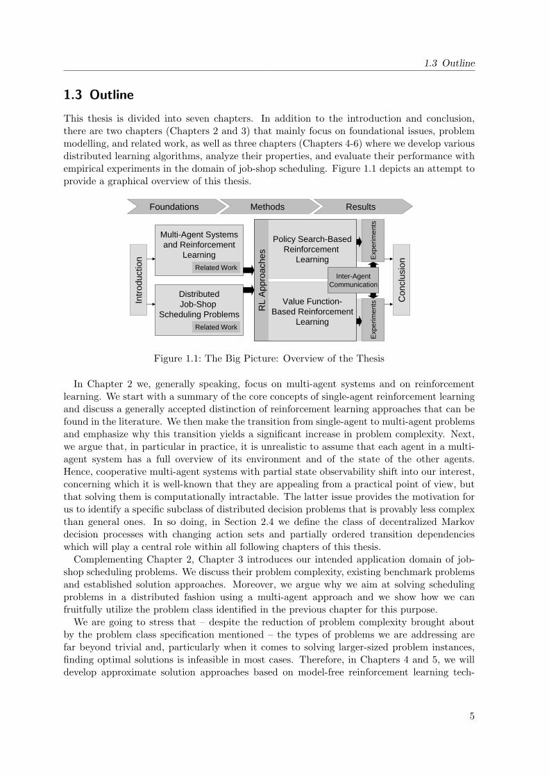
This thesis is divided into seven chapters. In addition to the introduction and conclusion,there are two chapters (Chapters 2 and 3) that mainly focus on foundational issues, problemmodelling, and related work, as well as three chapters (Chapters 4-6) where we develop variousdistributed learning algorithms, analyze their properties, and evaluate their performance withempirical experiments in the domain of job-shop scheduling. Figure 1.1 depicts an attempt toprovide a graphical overview of this thesis.
Foundations Methods Results
Intr
oduc
tion
Multi-Agent Systemsand Reinforcement
Learning
DistributedJob-Shop
Scheduling ProblemsRelated Work
Related WorkR
L A
ppro
ache
s
Policy Search-BasedReinforcement
Learning
Value Function-Based Reinforcement
Learning
Con
clus
ionE
xper
imen
tsE
xper
imen
ts
Inter-AgentCommunication
Figure 1.1: The Big Picture: Overview of the Thesis
In Chapter 2 we, generally speaking, focus on multi-agent systems and on reinforcementlearning. We start with a summary of the core concepts of single-agent reinforcement learningand discuss a generally accepted distinction of reinforcement learning approaches that can befound in the literature. We then make the transition from single-agent to multi-agent problemsand emphasize why this transition yields a significant increase in problem complexity. Next,we argue that, in particular in practice, it is unrealistic to assume that each agent in a multi-agent system has a full overview of its environment and of the state of the other agents.Hence, cooperative multi-agent systems with partial state observability shift into our interest,concerning which it is well-known that they are appealing from a practical point of view, butthat solving them is computationally intractable. The latter issue provides the motivation forus to identify a specific subclass of distributed decision problems that is provably less complexthan general ones. In so doing, in Section 2.4 we define the class of decentralized Markovdecision processes with changing action sets and partially ordered transition dependencieswhich will play a central role within all following chapters of this thesis.
Complementing Chapter 2, Chapter 3 introduces our intended application domain of job-shop scheduling problems. We discuss their problem complexity, existing benchmark problemsand established solution approaches. Moreover, we argue why we aim at solving schedulingproblems in a distributed fashion using a multi-agent approach and we show how we canfruitfully utilize the problem class identified in the previous chapter for this purpose.
We are going to stress that – despite the reduction of problem complexity brought aboutby the problem class specification mentioned – the types of problems we are addressing arefar beyond trivial and, particularly when it comes to solving larger-sized problem instances,finding optimal solutions is infeasible in most cases. Therefore, in Chapters 4 and 5, we willdevelop approximate solution approaches based on model-free reinforcement learning tech-
5
1 Introduction
niques by means of which we target at finding near-optimal solutions within reasonable time.In Chapter 4, we develop two distributed learning algorithms that are tailored for solvingapproximately single instances of decentralized decision processes and that exploit the charac-teristics of the problem class with changing action sets we identified before. These algorithmsperform a directed search in the space of policies the agents can represent and comply withcertain convergence properties. By contrast, in Chapter 5, we develop decentralized learningalgorithms that enable each agent to aim at determining a so-called value function for theproblem at hand from which a corresponding behavior can easily be derived. Moreover, ourgoal here is also on the issue of generalization which means that the agents learn behavior poli-cies that capture general problem-solving knowledge and, hence, can be successfully appliedfor altered or entirely different problem settings as well.
What is common to the investigations we make in both chapters mentioned previously isthat all approaches suggested rely on learning agent behaviors that can be described as purelyreactive, that is that the agents do not explicitly take into account their histories and do notspecifically address certain inter-agent dependencies. With the aim of enhancing the capabili-ties of purely reactively acting and learning agents, in Chapter 6, we study two approaches thatenable the agents to make more deliberate decisions. In particular, we are going to utilize com-munication between agents as a tool to resolve certain dependencies between agents. In thischapter as well as in the two preceding chapters, we empirically evaluate all the approachesproposed in the context of our targeted application domain: We model intricate job-shopscheduling problems as multi-agent problems, make the agents learn good scheduling poli-cies, and evaluate their performance using various established job-shop scheduling benchmarkproblems.
6
2 Single- and Multi-Agent ReinforcementLearning
One of the general aims of machine learning is to produce intelligent software systems, some-times called agents, by a process of learning and evolving. For the notion of an agent, however,there exists no generally accepted formal definition. According to Russell and Norvig (2003),“An agent is anything that can be viewed as perceiving its environment through sensors andacting upon that environment through actuators.” Agents are typically presumed to inhabitsome environment within which they have to strive for fulfilling some specific task. To do so,they must sequentially take decisions which actions to execute next, they ought to try to adapttheir policies of actions such that to behave optimally, and they may be required to reasonabout the existence of other agents with which to cooperate or compete.
In this chapter, we will start off (Section 2.1) by presenting the idea of reinforcement learningwhich represents one of the most popular frameworks for modelling intelligent agents and formaking them learn to solve a given task by repeatedly sensing and acting within their environ-ment. Subsequently, in Section 2.2 we will draw a bow from systems with single agents to thosewith multiple agents that collectively, yet independently must learn to achieve a common goal.Since, typically, in a multi-agent system not every agent gets hold of a global view over theentire environment including other agents, we specifically have to address the issue of partialobservability: To this end, we summarize the framework of decentralized partially observableMarkov decision processes (DEC-POMDPs, Bernstein et al., 2002), which is frequently usedfor modelling multi-agent problems (Section 2.3). Since general DEC-POMDPs are known tobe intractable except for the smallest problem sizes, in Section 2.4 we propose a sub-class ofsuch problems that builds the foundation for most of the ideas and methods to be presentedin the remainder of this thesis. Specifically, this sub-class is well suited to model a wide rangeof practical multi-agent problems, including the scheduling tasks that are in the particularcenter of our interest, and solving problem instances of this class is provably less complex thansolving general DEC-POMDPs. We end this chapter by a review of related work in Section2.5.
2.1 The Reinforcement Learning Framework
Reinforcement learning (RL, Sutton and Barto, 1998) follows the idea that an autonomouslyacting agent obtains its behavior policy through repeated interaction with its environment ona trial-and-error basis.
In each time step an RL agent observes the environmental state and makes a decision fora specific action, which, on the one hand, may incur some immediate reward (also calledreinforcement) generated by the agent’s environment and, on the other hand, transfers theagent into some successor state. The agent’s goal is not to maximize the immediate reward,but its long-term, expected reward. To do so, it must learn a decision policy that is used to
7
2 Single- and Multi-Agent Reinforcement Learning
determine the best action for a given state. Such a policy is a function that maps the currentstate the agent finds itself in to an action from a set of viable actions.
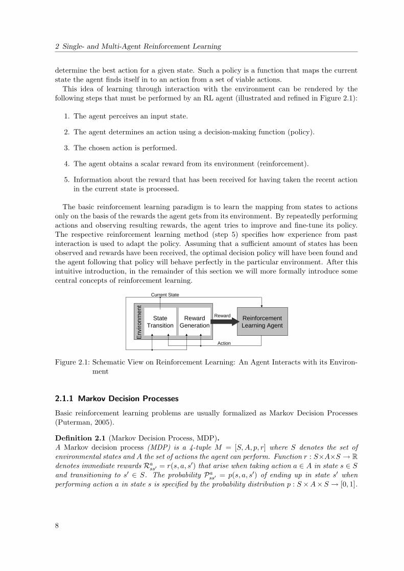
This idea of learning through interaction with the environment can be rendered by thefollowing steps that must be performed by an RL agent (illustrated and refined in Figure 2.1):
1. The agent perceives an input state.
2. The agent determines an action using a decision-making function (policy).
3. The chosen action is performed.
4. The agent obtains a scalar reward from its environment (reinforcement).
5. Information about the reward that has been received for having taken the recent actionin the current state is processed.
The basic reinforcement learning paradigm is to learn the mapping from states to actionsonly on the basis of the rewards the agent gets from its environment. By repeatedly performingactions and observing resulting rewards, the agent tries to improve and fine-tune its policy.The respective reinforcement learning method (step 5) specifies how experience from pastinteraction is used to adapt the policy. Assuming that a sufficient amount of states has beenobserved and rewards have been received, the optimal decision policy will have been found andthe agent following that policy will behave perfectly in the particular environment. After thisintuitive introduction, in the remainder of this section we will more formally introduce somecentral concepts of reinforcement learning.
Env
ironm
ent
StateTransition
RewardGeneration
ReinforcementLearning Agent
Action
Current State
Reward
Figure 2.1: Schematic View on Reinforcement Learning: An Agent Interacts with its Environ-ment
2.1.1 Markov Decision Processes
Basic reinforcement learning problems are usually formalized as Markov Decision Processes(Puterman, 2005).
Definition 2.1 (Markov Decision Process, MDP).A Markov decision process (MDP) is a 4-tuple M = [S,A, p, r] where S denotes the set ofenvironmental states and A the set of actions the agent can perform. Function r : S×A×S → Rdenotes immediate rewards Rass′ = r(s, a, s′) that arise when taking action a ∈ A in state s ∈ Sand transitioning to s′ ∈ S. The probability Pass′ = p(s, a, s′) of ending up in state s′ whenperforming action a in state s is specified by the probability distribution p : S×A×S → [0, 1].
8
2.1 The Reinforcement Learning Framework
For MDPs, the Markov property assures that the transition from s to s′ and the correspond-ing payout of reward Rass′ depends only on the starting state s and the action a taken, not onthe history of previous states and actions.
The behavior of the agent that interacts with its environment modelled as an MDP isspecified in terms of a policy function that is defined as follows.
Definition 2.2 (Policy (MDP case)).Given an MDP according to Definition 2.1, an agent’s policy π : S × A → [0, 1] specifies aprobability distribution over actions, where π(s, a) tells the probability of executing action a instate s. In this general case, this mapping from state-action pairs to probabilities is called astochastic policy.
A special case of a general, stochastic policy is a deterministic one which, for a given states, always picks the same action a and, hence, is written as π : S → A.
2.1.2 Learning Optimal Behavior
When interacting with the MDP, an RL agent passes through a sequence of states s(t), thatare coupled to one another by the transition probabilities Pa(t)
s(t),s(t+1), and receives a sequence
of immediate rewards r(t) = Ra(t)s(t),s(t+1). The goal of reinforcement learning is to maximize
the expected value E[Rt|s0, π] of the discounted sum
Rt =∞∑k=0
γtr(t+ k) (2.1)
of rewards the agent obtains over time, where γ ∈ [0, 1) is a factor that determines to whichamount future rewards are discounted compared to immediate ones.
When conditioned on some specific state s ∈ S, the expected value mentioned is called thevalue V π of state s under policy π and is recursively defined as
V π(s) = E[Rt|st = s, π]
=∑a∈A
π(s, a)∑s′∈SPass′(Rass′ + γV π(s′)). (2.2)
Accordingly, function V π is called the value function for policy π.In a similar manner, the value Qπ(s, a) of a state-action pair is defined, which is meant to
express the expected return after taking action a in state s and following policy π subsequently:
Qπ(s, a) = E[Rt|st = s, at = a, π]
=∑s′∈SPass′(Rass′ + γV π(s′)) (2.3)
In stochastic shortest path problems, the discount factor γ can be safely set to 1 because theexistence of a termination state sf is assumed. Once the agent reaches that state it remainsthere and receives no further rewards. Problems of that type are structured such that reachingsf is inevitable. Consequently, the goal is to reach the final state with maximal expectedreward1.
1Reinforcement learning literature uses the terms rewards and costs interchangeably where costs, intuitively,correspond to negative rewards. Hence, if the goal is to get to a terminal state under maximal reward, thiscould be formulated also as getting there under minimal costs.
9
2 Single- and Multi-Agent Reinforcement Learning
During learning the agent is in search of an optimal policy π? that outperforms all otherpolicies π in being capable of accumulating as much reward as possible. It has been shown(Bertsekas and Tsitsiklis, 1996) that for each MDP there exists an optimal policy π? such thatfor any policy π it holds V π?(s) ≥ V π(s) for all states s ∈ S. If we assume to be in possessionof an “optimal” value function V ?, it is easy to infer the corresponding optimal (deterministic)policy by exploiting the value function greedily according to
π?(s) = arg maxa∈A
∑s′∈SPass′(Rass′ + γV ?(s′)).
2.1.3 On Actors and Critics
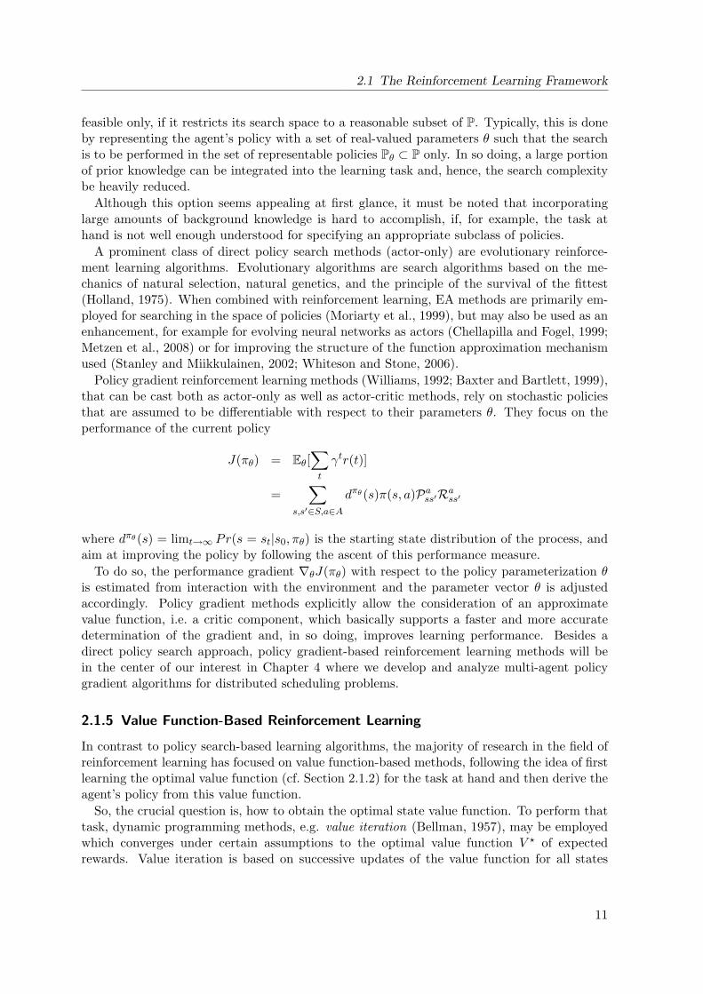
Considering the basic enumeration of steps a reinforcement learning agent performs (cf. thebeginning of Section 2.1), the most interesting part lies probably in step 5. Here, the agentis faced with the task of processing recent experience to obtain an improved version of itsbehavior policy. In order to coarsely distinguish different approaches for achieving that, theactor-critic architecture can be employed (Witten and Corbin, 1973; Barto et al., 1983).
Env
ironm
ent
StateTransition
RewardGeneration
RL
Age
nt
Actor(Policy)
Critic(e.g. ValueFunction)
Action a
State s
Reward r
determines / influences
Figure 2.2: The Actor-Critic Architecture
In actor-critic methods it is assumed that there are separate memory structures for theaction-taking part of the agent, i.e. the policy (actor), and a component, the critic, thatmonitors the performance of the actor and determines when and how the policy ought to bechanged. The critic very often takes the form of a value function.
Building upon the presence or absence of these two components, Heidrich-Meisner et al.(2007) distinguish between actor-only, actor-critic, and critic-only methods. Because the dis-tinction between the former two is rather subtle, in this thesis, we adopt a slightly differentview and differentiate between the following:
Policy Search-Based Methods comprise actor-only and actor-critic variants and are charac-terized by the fact that an explicit representation of an agent’s policy is present.
Value Function-Based Methods correspond to critic-only methods in that they basically relyon learning a value function and on (implicitly) inducing a policy from this function.
As the thesis at hand deals with both types of learning systems, we provide some correspondingfoundations in the next two subsections.
2.1.4 Policy Search-Based Reinforcement Learning
A policy search-based reinforcement learning agent employs an explicit representation of itsbehavior policy and aims at improving it by searching the space P of possible policies. This is
10
2.1 The Reinforcement Learning Framework
feasible only, if it restricts its search space to a reasonable subset of P. Typically, this is doneby representing the agent’s policy with a set of real-valued parameters θ such that the searchis to be performed in the set of representable policies Pθ ⊂ P only. In so doing, a large portionof prior knowledge can be integrated into the learning task and, hence, the search complexitybe heavily reduced.
Although this option seems appealing at first glance, it must be noted that incorporatinglarge amounts of background knowledge is hard to accomplish, if, for example, the task athand is not well enough understood for specifying an appropriate subclass of policies.
A prominent class of direct policy search methods (actor-only) are evolutionary reinforce-ment learning algorithms. Evolutionary algorithms are search algorithms based on the me-chanics of natural selection, natural genetics, and the principle of the survival of the fittest(Holland, 1975). When combined with reinforcement learning, EA methods are primarily em-ployed for searching in the space of policies (Moriarty et al., 1999), but may also be used as anenhancement, for example for evolving neural networks as actors (Chellapilla and Fogel, 1999;Metzen et al., 2008) or for improving the structure of the function approximation mechanismused (Stanley and Miikkulainen, 2002; Whiteson and Stone, 2006).
Policy gradient reinforcement learning methods (Williams, 1992; Baxter and Bartlett, 1999),that can be cast both as actor-only as well as actor-critic methods, rely on stochastic policiesthat are assumed to be differentiable with respect to their parameters θ. They focus on theperformance of the current policy
J(πθ) = Eθ[∑t
γtr(t)]
=∑
s,s′∈S,a∈Adπθ(s)π(s, a)Pass′Rass′
where dπθ(s) = limt→∞ Pr(s = st|s0, πθ) is the starting state distribution of the process, andaim at improving the policy by following the ascent of this performance measure.
To do so, the performance gradient ∇θJ(πθ) with respect to the policy parameterization θis estimated from interaction with the environment and the parameter vector θ is adjustedaccordingly. Policy gradient methods explicitly allow the consideration of an approximatevalue function, i.e. a critic component, which basically supports a faster and more accuratedetermination of the gradient and, in so doing, improves learning performance. Besides adirect policy search approach, policy gradient-based reinforcement learning methods will bein the center of our interest in Chapter 4 where we develop and analyze multi-agent policygradient algorithms for distributed scheduling problems.
2.1.5 Value Function-Based Reinforcement Learning
In contrast to policy search-based learning algorithms, the majority of research in the field ofreinforcement learning has focused on value function-based methods, following the idea of firstlearning the optimal value function (cf. Section 2.1.2) for the task at hand and then derive theagent’s policy from this value function.
So, the crucial question is, how to obtain the optimal state value function. To perform thattask, dynamic programming methods, e.g. value iteration (Bellman, 1957), may be employedwhich converges under certain assumptions to the optimal value function V ? of expectedrewards. Value iteration is based on successive updates of the value function for all states
11
2 Single- and Multi-Agent Reinforcement Learning
s ∈ S according toVk+1(s) = maxa∈A
∑s′∈SPass′(Rass′ + γVk(s′)), (2.4)
where index k denotes the sequence of approximated versions of V , until convergence to V ? isreached.
As a convenient shorthand notation, the operator T is used to denote a mapping betweencost-to-go functions according to Equation 2.4, i.e. (TVk)(s) = Vk+1(s) for all s ∈ S.
Speaking in terms of state-action values, i.e. Q values, using relation 2.3 and knowing thatBellman’s equation can be interpreted as V ?(s) = maxa∈A(s)Q
?(s, a), the value iteration algo-rithm from above can be written as
Qk+1(s, a) =∑s′∈SPass′(Rass′ + γ max
b∈A(s′)Qk(s′, b))
and, again, in operator notation this update scheme is abbreviated as (HQk)(s, a) = Qk+1(s, a)for all states and actions.
If there are no explicit transition model p of the environment and of the reward structure ravailable, Q learning is one of the reinforcement learning methods of choice to learn a state-action value function for the problem at hand (Watkins and Dayan, 1992). It updates directlythe estimates for the values of state-action pairs according to
Q(s, a) = (1− α)Q(s, a) + α(Rass′ + γmaxb∈A(s′)Q(s′, b)) (2.5)
where α denotes the learning rate and where the successor state s′ and the immediate rewardRass′ are generated by simulation or by interaction with a real process. For the case of finitestate and action spaces where the Q function can be represented using a look-up table, thereare convergence guarantees that say that Q learning converges to the optimal value functionQ?, assumed that all state-action pairs are visited infinitely often and that α diminishes appro-priately. Given convergence to Q?, the optimal policy π? can be induced by greedy exploitationof Q according to
π?(s) = arg maxa∈A(s)
Q?(s, a).
As outlined, the determination of an optimal state value function is crucial to most rein-forcement learning methods. Intending to show the functioning of some new RL technique inprinciple, one usually chooses typical benchmark problems (grid worlds) that are very limitedin terms of state and action space size. In those cases, having to deal with only a finite num-ber of states, it is feasible to store V (s) for each single state s ∈ S explicitly using a tabularfunction representation with |S| table entries. However, interesting reinforcement learningproblems have typically large, high-dimensional or even continuous state spaces, such thatcomputational and/or memory limitations inhibit the use of a tabular function representation.Instead, the employment of a function approximator becomes inevitable. Thus, we have toturn to “suboptimal” methods that target the evaluation and approximation of the optimalvalue function V ?(s) or Q?(s, a): We replace the optimal value function by an appropriateapproximation V (s, w), where w determines the set of the approximator’s parameters. In par-ticular, our focus will be on the use of neuro-dynamic approaches, where multilayer perceptron(MLP) neural networks are used as approximation architecture (Bertsekas and Tsitsiklis, 1996)which have shown to be a as a suitable and robust technique to approximate V ?.
12
2.2 From One to Many Agents
Networks of this type are known to be capable of representing any function that is continu-ous and closed on a bounded set arbitrarily close (Hornick et al., 1989), and they feature goodgeneralization capabilities. Although most theoretical results regarding the convergence be-havior of RL algorithms do not generally hold in the presence of value function approximation,impressive results could be obtained in the past, for example Tesauro’s milestone TD-Gammon(Tesauro, 1995).
Value iteration and Q learning, as outlined in this section, are just two prominent examplesfor a model-based and model-free reinforcement learning method, respectively. Research inRL, however, has generated a variety of methods that extend those well-known optimizationtechniques, aiming at applicability also in situations where large state spaces must be handledor where the absence of a transition model p and reward model r prevent the usage of simplevalue iteration. It is beyond the scope of this thesis to provide a comprehensive review onprogress and state of the art in RL. Instead, in later chapters, we will selectively relate ourwork to other well-known reinforcement learning algorithms and, if needed, briefly describethem.
Value function-based reinforcement learning methods will be in the center of our interestin Chapter 5 where we develop and deploy multi-agent reinforcement learning algorithms fordistributed scheduling problems.
2.2 From One to Many Agents
As pointed out by Littman (1994), no agent lives in a vacuum, but typically must interactwith other agents to achieve its goals. Distributed artificial intelligence (Weiss, 1999) is thesubfield of artificial intelligence that focuses on complex systems that are inhabited by multipleagents. The main goal of research in this area is to provide principles for the construction andapplication of multi-agent systems as well as means for coordinating the behavior of multipleindependent agents (Stone and Veloso, 2000).
Taking the step from a single-agent to a multi-agent system brings about significant changesin several aspects:
• From an individual agent’s point of view, the environment’s dynamics can no longer beinfluenced by itself only, but also by other agents taking their actions. This superimposeswith the uncertainty of the environment.
• The presence of other agents may require an agent to explicitly reason about their goals,actions, and to, eventually, coordinate appropriately.
• In addition to the single-agent temporal credit assignment problem, the multi-agentcredit assignment problem arises, which corresponds to answering the question of whoseagent’s local action contributed how much to a (corporate) success.
• When multiple agents learn and, hence, adapt their behavior in parallel, each individualagent faces the difficulty of learning in a non-stationary environment. Consequently,convergence guarantees, such as the convergence of the Q learning mentioned in Section2.1.5, may no longer hold.
In the following, we will approach these challenges from different sides. We start off byproviding a coarse classification of multi-agent systems and also discuss their relevance forpractical applications.
13
2 Single- and Multi-Agent Reinforcement Learning
2.2.1 Cooperative and Non-Cooperative Multi-Agent Systems
The literature on multi-agent systems makes a distinction regarding the level of cooperativenessof the agents inhabiting the same environment (Tan, 1993). Much work has been devoted onsystems with agents with competing or opposing goals, meaning that the reward functions ofthe agents are coupled in a complementary way: If one agent succeeds (e.g. gets a large reward),then the other one fails (e.g. gets a large negative reward). Such multi-agent systems havefrequently been modelled as Markov Games (Filar and Vrieze, 1996), in particular as zero-sum games, and a number of corresponding multi-agent reinforcement learning algorithmshave been suggested (Littman, 1994; Tesauro, 2003). Assuming full knowledge of the actionstaken by the opponent agent, those algorithms are typically guaranteed to converge to optimalsolutions. Moreover, extensions to those algorithms yielding faster learning progress weresuggested while still featuring guaranteed (Bikramjit et al., 2001) or approximate convergence(Brafman and Tennenholtz, 2001).
By contrast, in the universal case of general multi-agent systems each agent possesses its own,arbitrary reward function which may be entirely unrelated to the rewards other agents receive.Fundamental work for this realm of problems, sometimes referred to as general-sum games,was done by Hu and Wellman (1998, 2003) who developed the Nash-Q learning algorithmwith certain appealing theoretical properties (Bowling, 2000), but assumed an environmentwhere each agent has full knowledge over the actions taken by other agents. Aiming at thereduction of necessary preconditions to be met for this algorithm to be applicable, Littman(2001) proposed the Friend-or-Foe Q learning algorithm, which, however, requires every otheragent to be classified as cooperative or competitive a priori, and Greenwald and Hall (2003)developed correlated Q learning which generalizes Nash-Q and FoF-Q.
Completing the distinction started at the beginning of this section, we emphasize that thecase of multi-agent systems with cooperative agents which collectively aim at achieving acommon goal (so far, we briefly reviewed algorithms for competing agents only) is to be foundvery frequently in practical applications and, thus, of special importance. The thesis at handtargets cooperative multi-agent systems exclusively which is why in Section 2.3 we are goingto focus in detail on such problems. Prior to this, we shortly highlight the relevance of multi-agent systems research for practice by paying tribute to a number of successful applicationsand relevant industrial problems.
2.2.2 Application Fields of Learning Multi-Agent Systems
There is a variety of application fields for multi-agent systems and, what is of special interestto us, multi-agent reinforcement learning systems. We here provide only a brief and, for sure,incomplete overview of practical applications for learning approaches used in the scope ofcooperative multi-agent systems. Reinforcement learning and related approaches have beenapplied to optimize agent behavior in the scope of
• mobile telephony (e.g. for channel allocation (Singh and Bertsekas, 1997) or ad-hoc net-works (Chang et al., 2004)),
• network technology (e.g. for data packet routing (Boyan and Littman, 1994; Ferra et al.,2003)),
• elevator control (e.g. for adaptive elevator dispatching (Barto and Crites, 1996)),
14
2.3 Cooperative Multi-Agent Systems with Partial Observability
• energy and oil distribution (e.g. for electric power generation networks (Schneider et al.,1999) or for optimizing pipeline operations (Mora et al., 2008)),
• computing power management (e.g. for load balancing across servers (Tumer and Lawson,2003), for distributed computing (Tesauro et al., 2005), or for constrained job dispatchingin mainframe systems (Vengerov and Iakovlev, 2005)),
• autonomous robots (e.g. for robotic soccer (Riedmiller and Merke, 2003; Gabel et al.,2006; Riedmiller and Gabel, 2007) or for exploration of unknown territory (Low et al.,2008)) and computer games (e.g. for first-person shooter games (Smith et al., 2007)),
• rescue operations (e.g. for enabling units to decide independently which sites to searchand secure (Settembre et al., 2008)),
• or surveillance and security tasks (e.g. for distributed sensor networks (Marecki et al.,2008) or for patrolling tasks (Santana et al., 2004) or for military applications (Pitaet al., 2008)).
This numeration of mostly real-life applications misses another important area – the field ofproduction planning and factory optimization, where machines may act independently with thegoal of achieving maximal joint productivity – which shall move into the center of our interestin the successive chapters. Before we explore this application and related work in more detail(Chapter 3), we devote the following sections to providing a more fine-grained categorizationof cooperative multi-agent systems as well as to the identification of an appealing model forlearning in multi-agent systems.
2.3 Cooperative Multi-Agent Systems with Partial Observability
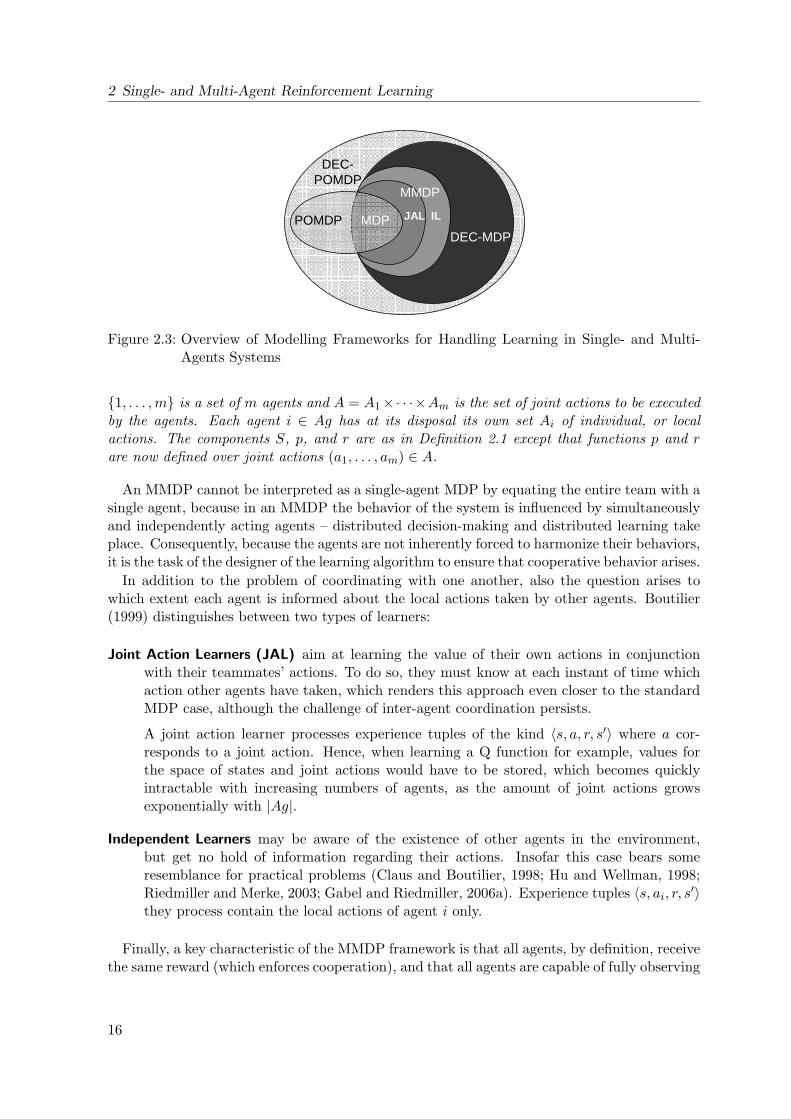
Speaking about different kinds of multi-agent systems, up to this point we assumed that eachagent possesses full knowledge over the global system state, i.e. it is aware not just of itsown local state, but also of the local states of all other agents as well. Moreover, decision-making for an agent is simplified, if it has full or at least partial information about the actionsits teammates are taking. Especially in the light of practical applications, these assumptionsappear rather unrealistic, which is why a more fine-grained classification of multi-agent systemswith respect to the observation capabilities of the agents is required. In the following, we aregoing to focus on fully cooperative multi-agent systems and explore three specific dimensionsalong which the observability of the environment and of the other agents can be restricted.This discussion is accompanied by Figure 2.3 which gives a comprehensive overview of thecorresponding frameworks and formal models.
2.3.1 The Multi-Agent Markov Decision Process Model
Boutilier (1999) introduced a straightforward extension of standard Markov decision processesto the multi-agent case. He assumes that a collection of agents controls the system by theirindividual actions: The effects of one agent’s actions blend with those taken by others, whileall agents share the same reward function.
Definition 2.3 (Multi-Agent Markov Decision Process, MMDP).A multi-agent Markov decision process (MMDP) is a 5-tuple M = [Ag, S,A, p, r] where Ag =
15
2 Single- and Multi-Agent Reinforcement Learning
DEC-POMDP
POMDP MDPDEC-MDP
MMDP
JAL IL
Figure 2.3: Overview of Modelling Frameworks for Handling Learning in Single- and Multi-Agents Systems
1, . . . ,m is a set of m agents and A = A1×· · ·×Am is the set of joint actions to be executedby the agents. Each agent i ∈ Ag has at its disposal its own set Ai of individual, or localactions. The components S, p, and r are as in Definition 2.1 except that functions p and rare now defined over joint actions (a1, . . . , am) ∈ A.
An MMDP cannot be interpreted as a single-agent MDP by equating the entire team with asingle agent, because in an MMDP the behavior of the system is influenced by simultaneouslyand independently acting agents – distributed decision-making and distributed learning takeplace. Consequently, because the agents are not inherently forced to harmonize their behaviors,it is the task of the designer of the learning algorithm to ensure that cooperative behavior arises.
In addition to the problem of coordinating with one another, also the question arises towhich extent each agent is informed about the local actions taken by other agents. Boutilier(1999) distinguishes between two types of learners:
Joint Action Learners (JAL) aim at learning the value of their own actions in conjunctionwith their teammates’ actions. To do so, they must know at each instant of time whichaction other agents have taken, which renders this approach even closer to the standardMDP case, although the challenge of inter-agent coordination persists.
A joint action learner processes experience tuples of the kind 〈s, a, r, s′〉 where a cor-responds to a joint action. Hence, when learning a Q function for example, values forthe space of states and joint actions would have to be stored, which becomes quicklyintractable with increasing numbers of agents, as the amount of joint actions growsexponentially with |Ag|.
Independent Learners may be aware of the existence of other agents in the environment,but get no hold of information regarding their actions. Insofar this case bears someresemblance for practical problems (Claus and Boutilier, 1998; Hu and Wellman, 1998;Riedmiller and Merke, 2003; Gabel and Riedmiller, 2006a). Experience tuples 〈s, ai, r, s′〉they process contain the local actions of agent i only.
Finally, a key characteristic of the MMDP framework is that all agents, by definition, receivethe same reward (which enforces cooperation), and that all agents are capable of fully observing
16
2.3 Cooperative Multi-Agent Systems with Partial Observability
the global system state. In particular, the latter strongly restricts the applicability of the multi-agent Markov decision process model since this assumption rarely holds in practice. Insofar,the MMDP model has paved the way towards defining more powerful modelling mechanismsthat also cover partial state observability to which we will turn soon (Section 2.3.3). Summingup, the type of agents we will deal with in the remainder of this work can be characterized asindependent learners that are obstructed by several further constraining restrictions.
2.3.2 Partially Observable Markov Decision Processes
In the real world, an agent may not be able to accurately observe the current state of itsenvironment. This may be caused, for instance, by faulty or noisy sensors that disturb thetrue observation according to some probability distribution. Another reason may be thatthe agent’s observation capabilities are restricted to certain features of the world state only,which results in that the agent perceives certain different states as identical. In order tohandle problems such as uncertain observations or perceptual aliasing, the model of partiallyobservable Markov decision processes (POMDPs, cf. Figure 2.3) has been introduced whichextends the MDP model by considering observations and their probabilities of occurrencedepending on the current state.
Definition 2.4 (Partially Observable Markov Decision Processes, POMDP).A partially observable Markov decision process (POMDP) is a 6-tuple M = [S,A, p, r,Ω, O]where S, A, p, r are defined as for an MDP (Definition 2.1). The set of possible observationsthe agent can make is denoted by Ω, and O : S×A×S×Ω→ [0, 1] is a probability distributionover observations where O(s, a, s′, o) denotes the probability that the agent observes o ∈ Ω uponexecuting action a ∈ A in state s ∈ S and transitioning to s′ ∈ S.
In the thesis at hand, (single-agent) POMDPs are no further investigated since our maininterest is on multi-agent systems. We briefly refer to relevant and surveying literature (e.g. byLovejoy (1991), Kaelbling et al. (1998), or Timmer (2008)).
2.3.3 The Framework of Decentralized Markov Decision Processes
We are interested in systems with full decentralization: The system is cooperatively controlledby a group of independent decision makers which do not have a global view of the system stateand where none of the agents can influence the whole system state by its actions. Nevertheless,those agents share the same objectives and aim at maximizing the utility of the team asa whole. In order to study decentralized decision-making under the conditions mentioned,Bernstein et al. (2002) proposed the framework of decentralized partially observable Markovdecision processes.
Definition 2.5 (Decentralized Partially Observable Markov Decision Process). A decentral-ized partially observable Markov decision process (DEC-POMDP) is defined as a 7-tupleM = [Ag, S,A, p, r,Ω, O] with
• Ag = 1, . . . ,m as the set of agents,
• S as the set of world states
• A = A1 × ... × Am as the set of joint actions to be performed by the agents (a =(a1, . . . , am) ∈ A denotes a joint action that is made up of elementary actions ai takenby agent i),
17
2 Single- and Multi-Agent Reinforcement Learning
• p as the transition function with p(s, a, s′) denoting the probability that the system arrivesat state s′ upon executing joint action a in s,
• r as the reward function with r(s, a, s′) denoting the reward for executing a in s andtransitioning to s′,
• Ω = Ω1 × · · · × Ωm as the set of all observations of all agents (o = (o1, . . . , om) ∈ Ωdenotes a joint observation with oi as the observation for agent i),
• O as the observation function that determines the probability O(o1, . . . , om|s, a, s′) thatagent 1 through m perceive observations o1 through om upon the execution of a in s andentering s′.
For DEC-POMDPs it is assumed that the states possess the Markov property. This meansthat the next global state s′ depends only on the current state s and on the joint action aexecuted, but not on the history of states and actions:
Pr(st+1|at, st, at−1, st−1, . . . , a0, s0) = Pr(st+1|at, st).
The literature on DEC-POMDPs typically assumes that the world state can be factored intocomponents relating to individual agents. In so doing, it is possible to separate features of theworld state belonging to one agent from those that belong to others. Such a factorization isstrict in the sense that a single feature of the global state can correspond to one agent only.
Definition 2.6 (Factored DEC-POMDP).A factored, m-agent DEC-POMDP is defined such that the set S of states can be factored intom agent-specific components: S = S1 × · · · × Sm.
We refer to the agent-specific components si ∈ Si, ai ∈ Ai, and oi ∈ Ωi as the local state(also denoted as the partial view), local action and local observation of agent i, respectively.
Concerning the degree of observability, a number of cases must be distinguished. If theobservation function is defined in such a manner that each agent’s local observation alwaystruly identifies the global state, then the problem is said to be fully observable. In this case,which we will not consider any further, a DEC-POMDP effectively reduces to an MMDP(cf. Definition 2.3). The opposite extreme is when the agents do not obtain any informationat all related to the current state. Non-observing agents may be modelled by letting Ωi = ∅for all i. Between these two extreme cases, there are many nuances concerning the degree ofpartial state observability. A prominent special case – moving into our focus from now on – iswhen the joint observation of all agents collectively identifies the world state, which gives riseto the definition of DEC-MDPs:
Definition 2.7 (Decentralized Markov Decision Processes, DEC-MDP).A DEC-POMDP is said to be jointly observable, if the current state s is entirely determined bythe amalgamation of all agents’ observations: if O(o|s, a, s′) > 0, then Pr(s′|o) = 1. A DEC-POMDP that is jointly observable is called a decentralized Markov decision process (DEC-MDP).
Apparently, a DEC-POMDP generalizes a POMDP by allowing for controlling the systemstate in a decentralized manner using a set Ag of agents that each have a local view, and hence
18
2.3 Cooperative Multi-Agent Systems with Partial Observability
partial observability, on the system state only. In a similar manner, a DEC-MDP generalizesstandard Markov decision processes.
Notice, however, although the combination of the agents’ local observations tells the globalsystem state, each agent individually may still be uncertain regarding its own local state si.
Definition 2.8 (Locally Fully Observable DEC-MDP).A factored m-agent DEC-MDP has local full observability, if for all agents i and for all localobservations oi there is a local state si such that Pr(si|oi) = 1.
It is important to note that joint observability of a DEC-POMDP M (i.e. it is a DEC-MDP)in combination with local full observability (i.e. fully known local states) do not imply thatM is fully observable (i.e. that it was an MMDP). As a matter of fact, in many practicalmulti-agent systems it holds that the observations of all agents, when combined, reveal withcertainty the global state, and each such observation determines with certainty the partialview of an agent, but, none of the agents knows the complete state of the system – typicallyvast parts of the global state are hidden from each of the agents.
Figure 2.3 visualizes the relationships between the models defined so far and highlights howthe decentralized frameworks generalize and subsume the single-agent ones. In accordanceto the step towards decentralization taken, we may also define local and joint policies fordecentralized Markov decision processes:
Definition 2.9 (Local and Joint Policies, Deterministic and Reactive Local Policies).Given a decentralized (partially observable) Markov decision process according to Definitions2.6/2.7, a local policy πi of agent i is defined as a mapping from local sequences of observationsoi = oi,1, . . . , oi,t over Ωi to a probability distribution over actions from Ai, i.e. πi : Ωi ×Ai →[0, 1].
A joint policy π is defined as the tuple of m local policies, i.e. π = 〈π1, . . . , πm〉. Additionally,we define two special cases of general, stochastic local policies:
1. A deterministic local policy, for a given observation sequence oi, always picks the sameaction a ∈ Ai and, hence, is written as πi : Ωi → Ai.
2. A reactive local policy πi ignores the observation sequence oi and picks its action basedsolely on its most recent observation oi. Hence, it is written as πi : Ωi ×Ai → [0, 1].
We note that a local policy for agent i acting in a locally fully observable DEC-POMDP(Definition 2.8) is a mapping from sequences si ∈ Si of local states in agent i’s partial viewto local actions, i.e. πi : Si × Ai → [0, 1]. This differs from locally non-fully observable DEC-POMDPs where local policies are defined on top of sequences of local observations.
In the remainder of this thesis, we primarily consider multi-agent systems with joint fullobservability (DEC-MDPs), since a factorization of the world state is natural in many practicaland real-world problems. Right away, however, this ostensible simplification does not bringabout a reduction of the complexity of the problems considered, as we will see in the nextsection.
2.3.4 The Price of Decentralization
Research on distributed systems has pointed out that decentralizing control and observabilityamong agents has a significant impact on the complexity of solving a given problem. In
19
2 Single- and Multi-Agent Reinforcement Learning
particular, it is well-known that solving optimally a DEC-POMDP (and, equally, a DEC-MDP) is NEXP-complete2, even in the benign case of two agents: A non-deterministic Turingmachine requires O(2p(n)) time, with p(n) as an arbitrary polynomial and problem size n, andunlimited space for deciding such a problem (Bernstein et al., 2000).
On the one hand, this stands in clear contrast to the bounds for MDPs (P-completeness,i.e. decidable by a deterministic Turing machine within O(p(n)) time, (Papadimitriou andTsitsiklis, 1987)) and for POMDPs (PSPACE-completeness, i.e. decidable by a deterministicTuring machine using O(p(n)) space, (Mundhenk et al., 2000)). On the other hand, thisincrease in complexity can be elucidated when considering that the size of an agent’s localpolicy grows exponentially with the number of observations it can make, because a localpolicy is a mapping from local observation histories to actions. Therefore, there are |Ai||Ωi|
T
possible policies, if we denote by T the time horizon considered. In order to solve the DEC-MDP at hand optimally, each agent j would be required to build a belief-state MDP for eachone of agent i’s local policies. The number of states in any of these belief-state MDPs wouldbe exponential in the number |Ωj | of observations agent j can make, as it must consider itsobservation histories. Although this argument is informal (for a formal reduction proof seeBernstein et al. (2000)), it hints to the doubly exponential complexity of this class of problems.
In this thesis, we address the intricacy of learning and acting in general decentralized Markovdecision processes by the following two orthogonal approaches.
Exploitation of Problem Structure Many practical problems exhibit some structure whoseexploitation may ease the task of finding solutions. In the subsequent section (Section2.4), we are going to identify a subclass of general DEC-MDPs that features regularitiesin the way the agents interact with one another. For this class, we can show thatthe complexity of optimally solving an instance of such a DEC-MDP is provably lowerthan the general problem. Moreover, this class is of high relevance for many real-worldapplications. Correspondingly, in Chapter 3 we show how it can be employed for problemsfrom the application field of production planning.
Approximate Solutions Even though a lower complexity class may be entered by sticking tocertain subclasses of the general problem, the computational complexity of a probleminstance of such a DEC-(PO)MDP may be still so high that optimally solving it isinfeasible. This holds, in particular, when intending to tackle problems of larger sizethat are of relevance for practical problems. Given these facts, our goal will be not todevelop optimal solution algorithms that are applicable to small problems only, but tolook for techniques capable of quickly obtaining approximate solutions in the vicinity ofthe optimum.
For this task, we will develop and utilize various model-free reinforcement learning ap-proaches in subsequent chapters. In contrast to offline planning algorithms which aimat finding optimal solutions in a model-based manner, reinforcement learning allows foremploying independently learning agents and, hence, for a full decentralization of theproblem.
2Also referred to as NEXPTIME-complete or NPEXP-complete, see Bovet and Crescenzi (1994) for details oncomplexity classes.
20
2.4 Decentralized Markov Decision Processes with Changing Action Sets
2.4 Decentralized Markov Decision Processes with ChangingAction Sets
The enormous computational complexity of solving decentralized cooperative Markov decisionprocesses conflicts with the fact that real-world tasks do typically have a considerable problemsize. In this section, we identify a new subclass of general DEC-MDPs whose complexity isprovably lower (NP-hard) and discuss its characteristics (Gabel and Riedmiller, 2008a).
2.4.1 On Transition Dependencies
Speaking about interactions between agents, one must distinguish between independent localactions (also called non-interacting) and dependent local actions (also called interacting ones).Independent actions influence the local state and observation of the agent only which is ex-ecuting those actions, whereas the local observations and state transitions of its teammatesremain unaffected. By contrast, dependent local actions interfere with other agents and havean influence on their local observations and transitions. We formalize this concept by definingtransition and observation independence.
Definition 2.10 (Transition and Observation Independence).A factored m-agent DEC-MDP is called (a) transition-independent and (b) observation-inde-pendent, if there exist functions (a) p1, . . . , pm and (b) O1, . . . , Om such that
(a) p(s′i|(s1, . . . , sm), (a1, . . . , am), (s′1, . . . , s′i−1, s
′i+1, . . . , s
′m)) = pi(s′i|si, ai)
(b) O(oi|(s1, . . . , sm), (a1, . . . , am), (s′1, . . . , s′m), (o1, . . . , oi−1, oi+1, . . . , om)) = Oi(oi|si, ai, s′i)
for all agents i = 1, . . . ,m.
Thus, transition independence implies that the new local state of agent i depends only onits previous local state and its recent local action. Consequently, the transition function p ofthe multi-agent system’s underlying MDP can be factored such that
p(s′1, . . . , s′m|(s1, . . . , sm), (a1, . . . , am)) = Πm
i=1pi(s′i|si, ai).
Similarly, observation independence means that the observation an agent i sees depends ex-clusively on i’s recent and new local state as well as on its action taken.
Clearly, transition and observation independence represent rather strong assumptions on amulti-agent system, implying that the agents act very much decoupled from one another andnever interfere.
Definition 2.11 (Reward Independence).A factored m-agent DEC-MDP is called reward-independent, if there is a local reward functionri : Si × Ai × Si → R for all i ∈ Ag as well as a function R : Rm → R that amalgamates theglobal reward value from the local ones, such that maximizing each ri individually also yieldsa maximization of R. Thus,
r((s1, . . . , sm), (a1, . . . , am), (s′1, . . . , s′m)) = R(r1(s1, a1, s
′1), . . . , rm(sm, am, s′m)))
and for all i ∈ Ag
ri(si, ai, s′i) ≤ ri(si, a′i, s′′i )
⇔ R(r1, . . . , ri(si, ai, s′i), . . . , rm) ≤ R(r1, . . . ri(si, a′i, s′′i ) . . . , rm).
21
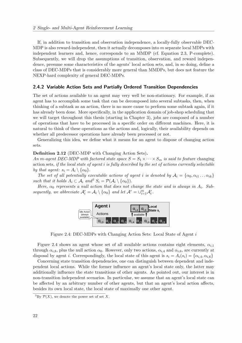
2 Single- and Multi-Agent Reinforcement Learning
If, in addition to transition and observation independence, a locally-fully observable DEC-MDP is also reward-independent, then it actually decomposes into m separate local MDPs withindependent learners and, hence, corresponds to an MMDP (cf. Equation 2.3, P-complete).Subsequently, we will drop the assumptions of transition, observation, and reward indepen-dence, presume some characteristics of the agents’ local action sets, and, in so doing, define aclass of DEC-MDPs that is considerably more general than MMDPs, but does not feature theNEXP-hard complexity of general DEC-MDPs.
2.4.2 Variable Action Sets and Partially Ordered Transition Dependencies
The set of actions available to an agent may very well be non-stationary. For example, if anagent has to accomplish some task that can be decomposed into several subtasks, then, whenthinking of a subtask as an action, there is no more cause to perform some subtask again, if ithas already been done. More specifically, in the application domain of job-shop scheduling thatwe will target throughout this thesis (starting in Chapter 3), jobs are composed of a numberof operations that have to be processed in a specific order on different machines. Here, it isnatural to think of these operations as the actions and, logically, their availability depends onwhether all predecessor operations have already been processed or not.
Generalizing this idea, we define what it means for an agent to dispose of changing actionsets.
Definition 2.12 (DEC-MDP with Changing Action Sets).An m-agent DEC-MDP with factored state space S = S1×· · ·×Sm is said to feature changingaction sets, if the local state of agent i is fully described by the set of actions currently selectableby that agent: si = Ai \ α0.
The set of all potentially executable actions of agent i is denoted by Ai = α0, αi1 . . . αiksuch that it holds Ai ⊂ Ai and3 Si = P(Ai \ α0).
Here, α0 represents a null action that does not change the state and is always in Ai. Sub-sequently, we abbreviate Ari = Ai \ α0 and let Ar = ∪mi=1Ari .
αi,1
Agent i
Actions
αi,0 αi,2 αi,3 αi,5 αi,6 αi,7 αi,8αi,4
αi,4 αi,6
available
LocalState siIdle Action
(alwaysavailable)
Figure 2.4: DEC-MDPs with Changing Action Sets: Local State of Agent i
Figure 2.4 shows an agent whose set of all available actions contains eight elements, αi,1through αi,8, plus the null action α0. However, only two actions, αi,4 and αi,6, are currently atdisposal by agent i. Correspondingly, the local state of this agent is si = Ai(si) = αi,4, αi,6
Concerning state transition dependencies, one can distinguish between dependent and inde-pendent local actions. While the former influence an agent’s local state only, the latter mayadditionally influence the state transitions of other agents. As pointed out, our interest is innon-transition independent scenarios. In particular, we assume that an agent’s local state canbe affected by an arbitrary number of other agents, but that an agent’s local action affects,besides its own local state, the local state of maximally one other agent.
3By P(X), we denote the power set of set X.
22
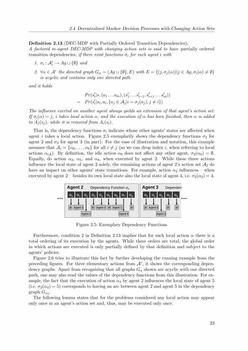
2.4 Decentralized Markov Decision Processes with Changing Action Sets
Definition 2.13 (DEC-MDP with Partially Ordered Transition Dependencies).A factored m-agent DEC-MDP with changing action sets is said to have partially orderedtransition dependencies, if there exist functions σi for each agent i with
1. σi : Ari → Ag ∪ ∅ and
2. ∀α ∈ Ar the directed graph Gα = (Ag ∪ ∅, E) with E = (j, σj(α))|j ∈ Ag, σi(α) 6= ∅is acyclic and contains only one directed path
and it holds
Pr(s′i|s, (a1 . . . am), (s′1 . . . s′i−1, s
′i+1 . . . s
′m))
= Pr(s′i|si, ai, aj ∈ Aj |i = σj(aj), j 6= i)
The influence exerted on another agent always yields an extension of that agent’s action set:If σi(α) = j, i takes local action α, and the execution of α has been finished, then α is addedto Aj(sj), while it is removed from Ai(si).
That is, the dependency functions σi indicate whose other agents’ states are affected whenagent i takes a local action. Figure 2.5 exemplarily shows the dependency functions σ2 foragent 2 and σ3 for agent 3 (in part). For the ease of illustration and notation, this exampleassumes that Ai = α0, . . . , α8 for all i 6= j (so we can drop index i, when referring to localactions αi,k). By definition, the idle action α0 does not affect any other agent, σ2(α0) = ∅.Equally, do action α3, α5, and α8, when executed by agent 2. While these three actionsinfluence the local state of agent 2 solely, the remaining actions of agent 2’s action set A2 dohave an impact on other agents’ state transitions. For example, action α2 influences – whenexecuted by agent 2 – besides its own local state also the local state of agent 4, i.e. σ2(α2) = 4.
Agent 2 Dependency Function σ2
α1α0 α2 α3 α5 α6 α7 α8α4
Agent 3
Agent 4
Agent 5 Agent 1
Agent 6
Ø Ø Ø Ø
… …
Agent 3 Dependen
α1α0 α2 α3 α4
Agent 6Ø Ø Ø
Agent 2
Figure 2.5: Exemplary Dependency Functions
Furthermore, condition 2 in Definition 2.13 implies that for each local action α there is atotal ordering of its execution by the agents. While these orders are total, the global orderin which actions are executed is only partially defined by that definition and subject to theagents’ policies.
Figure 2.6 tries to illustrate this fact by further developing the running example from thepreceding figures. For three elementary actions from Ar, it shows the corresponding depen-dency graphs. Apart from recognizing that all graphs Gα shown are acyclic with one directedpath, one may also read the values of the dependency functions from this illustration: For ex-ample, the fact that the execution of action α4 by agent 2 influences the local state of agent 5(i.e. σ2(α4) = 5) corresponds to having an arc between agent 2 and agent 5 in the dependencygraph Gα4 .
The following lemma states that for the problems considered any local action may appearonly once in an agent’s action set and, thus, may be executed only once.
23
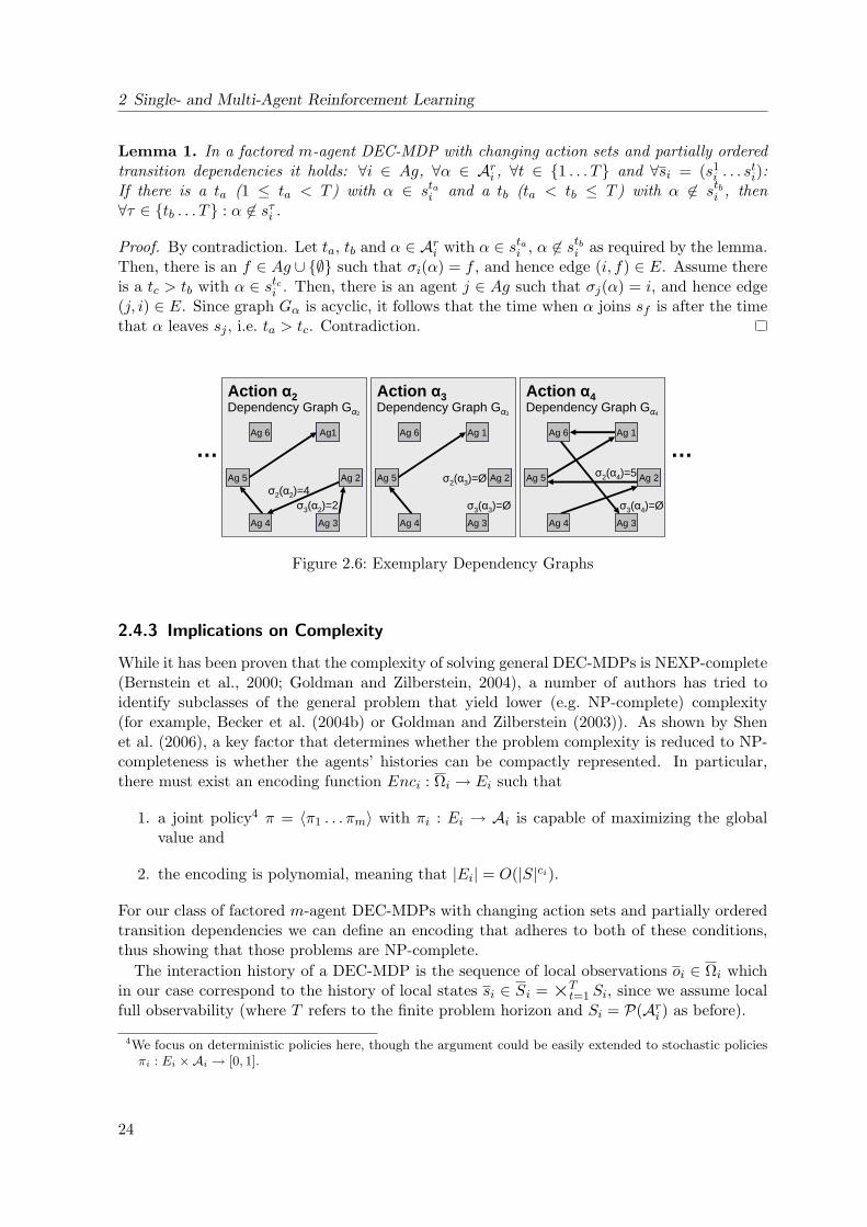
2 Single- and Multi-Agent Reinforcement Learning
Lemma 1. In a factored m-agent DEC-MDP with changing action sets and partially orderedtransition dependencies it holds: ∀i ∈ Ag, ∀α ∈ Ari , ∀t ∈ 1 . . . T and ∀si = (s1
i . . . sti):
If there is a ta (1 ≤ ta < T ) with α ∈ stai and a tb (ta < tb ≤ T ) with α 6∈ stbi , then∀τ ∈ tb . . . T : α 6∈ sτi .
Proof. By contradiction. Let ta, tb and α ∈ Ari with α ∈ stai , α 6∈ stbi as required by the lemma.Then, there is an f ∈ Ag ∪ ∅ such that σi(α) = f , and hence edge (i, f) ∈ E. Assume thereis a tc > tb with α ∈ stci . Then, there is an agent j ∈ Ag such that σj(α) = i, and hence edge(j, i) ∈ E. Since graph Gα is acyclic, it follows that the time when α joins sf is after the timethat α leaves sj , i.e. ta > tc. Contradiction.
Ag1
Ag 2
Ag 3Ag 4
Ag 5
Ag 6
Action α2Dependency Graph G
α2
Ag 1
Ag 2
Ag 3Ag 4
Ag 5
Ag 6
Action α3Dependency Graph G
α3
Ag 1
Ag 2
Ag 3Ag 4
Ag 5
Ag 6
Action α4Dependency Graph G
α4
σ2(α2)=4
σ2(α4)=5σ2(α3)=Ø
… …
σ3(α2)=2 σ3(α3)=Ø σ3(α4)=Ø
Ag1
Ag 2
Ag 3Ag 4
Ag 5
Ag 6 Ag 1
Ag 2
Ag 3Ag 4
Ag 5
Ag 6 Ag 1
Ag 2
Ag 3Ag 4
Ag 5
Ag 6
Figure 2.6: Exemplary Dependency Graphs
2.4.3 Implications on Complexity
While it has been proven that the complexity of solving general DEC-MDPs is NEXP-complete(Bernstein et al., 2000; Goldman and Zilberstein, 2004), a number of authors has tried toidentify subclasses of the general problem that yield lower (e.g. NP-complete) complexity(for example, Becker et al. (2004b) or Goldman and Zilberstein (2003)). As shown by Shenet al. (2006), a key factor that determines whether the problem complexity is reduced to NP-completeness is whether the agents’ histories can be compactly represented. In particular,there must exist an encoding function Enci : Ωi → Ei such that
1. a joint policy4 π = 〈π1 . . . πm〉 with πi : Ei → Ai is capable of maximizing the globalvalue and
2. the encoding is polynomial, meaning that |Ei| = O(|S|ci).
For our class of factored m-agent DEC-MDPs with changing action sets and partially orderedtransition dependencies we can define an encoding that adheres to both of these conditions,thus showing that those problems are NP-complete.
The interaction history of a DEC-MDP is the sequence of local observations oi ∈ Ωi whichin our case correspond to the history of local states si ∈ Si =×T
t=1 Si, since we assume localfull observability (where T refers to the finite problem horizon and Si = P(Ari ) as before).
4We focus on deterministic policies here, though the argument could be easily extended to stochastic policiesπi : Ei ×Ai → [0, 1].
24
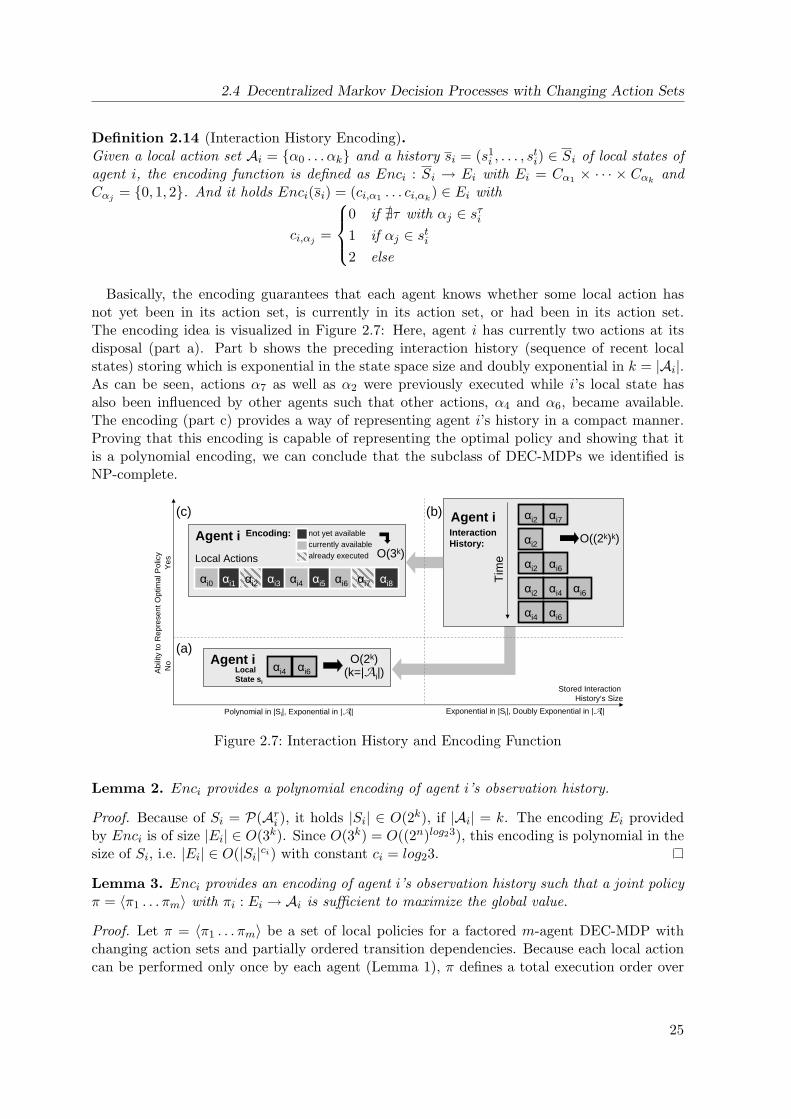
2.4 Decentralized Markov Decision Processes with Changing Action Sets
Definition 2.14 (Interaction History Encoding).Given a local action set Ai = α0 . . . αk and a history si = (s1
i , . . . , sti) ∈ Si of local states of
agent i, the encoding function is defined as Enci : Si → Ei with Ei = Cα1 × · · · × Cαk andCαj = 0, 1, 2. And it holds Enci(si) = (ci,α1 . . . ci,αk) ∈ Ei with
ci,αj =
0 if @τ with αj ∈ sτi1 if αj ∈ sti2 else
Basically, the encoding guarantees that each agent knows whether some local action hasnot yet been in its action set, is currently in its action set, or had been in its action set.The encoding idea is visualized in Figure 2.7: Here, agent i has currently two actions at itsdisposal (part a). Part b shows the preceding interaction history (sequence of recent localstates) storing which is exponential in the state space size and doubly exponential in k = |Ai|.As can be seen, actions α7 as well as α2 were previously executed while i’s local state hasalso been influenced by other agents such that other actions, α4 and α6, became available.The encoding (part c) provides a way of representing agent i’s history in a compact manner.Proving that this encoding is capable of representing the optimal policy and showing that itis a polynomial encoding, we can conclude that the subclass of DEC-MDPs we identified isNP-complete.
Agent iαi4 αi6Local
State si
O(2k)(k=|Ai|)
αi1
Agent i
Local Actions
αi0 αi2 αi3 αi5 αi6 αi7 αi8αi4
Encoding: not yet availablecurrently availablealready executed O(3k)
Agent i
αi4 αi6
Interaction History: O((2k)k)
Tim
e
αi2 αi4
αi2 αi6
αi2
αi6
αi2 αi7
Stored Interaction History‘s Size
Exponential in |Si|, Doubly Exponential in |Ai|Polynomial in |Si|, Exponential in |Ai|
Abi
lity
to R
epre
sent
Opt
imal
Pol
icy
Yes
No
(a)
(c) (b)
Figure 2.7: Interaction History and Encoding Function
Lemma 2. Enci provides a polynomial encoding of agent i’s observation history.
Proof. Because of Si = P(Ari ), it holds |Si| ∈ O(2k), if |Ai| = k. The encoding Ei providedby Enci is of size |Ei| ∈ O(3k). Since O(3k) = O((2n)log23), this encoding is polynomial in thesize of Si, i.e. |Ei| ∈ O(|Si|ci) with constant ci = log23.
Lemma 3. Enci provides an encoding of agent i’s observation history such that a joint policyπ = 〈π1 . . . πm〉 with πi : Ei → Ai is sufficient to maximize the global value.
Proof. Let π = 〈π1 . . . πm〉 be a set of local policies for a factored m-agent DEC-MDP withchanging action sets and partially ordered transition dependencies. Because each local actioncan be performed only once by each agent (Lemma 1), π defines a total execution order over
25
2 Single- and Multi-Agent Reinforcement Learning
the elements of Ari for all agents i. Thus, each local policy must allow for realizing any possiblesuch order. Since Ei contains the historical information which actions α ∈ Ari have alreadybeen executed, each πi can select the next αx ∈ Ai to be executed depending on ei: If αx ∈ si(si as current action set), i.e. ei,x = 1, then that action is taken, otherwise (αx is not yet inthe action set, ci,x = 0) the null action α0 is selected.
Because deciding a polynomially encodable DEC-MDP is NP-complete (Shen et al., 2006),solving a factored m-agent DEC-MDP with changing action sets and partially ordered transi-tion dependencies is so, also.
Theorem 1. Solving a factored m-agent DEC-MDP with changing action sets and partiallyordered transition dependencies is NP-complete.
Proof. This follows directly from the fact that deciding a polynomially encodable DEC-MDPis NP-complete (Shen et al., 2006) and from Lemma 2 and 3.
2.4.4 Example Applications
Factored DEC-MDPs with changing action sets and partially ordered transition dependenciesmay seem to represent a small set of domains, but it turns out that the class of problemswe address is quite general. This class of problems involves cooperative agents, each havingits local view and its local set of tasks to perform, with specific structured interactions anddependencies between them. Those dependencies can model the locking of a shared resource aswell as temporal enabling constraints, both of which arise frequently in practical applications.
It should be noted that distributed problem solving in practice is often characterized by afactored system state description where the agents base their decisions on local observations.Also, our assumptions that local actions may influence the state transitions of maximallyone other agent and that any action has to be performed only once are frequently fulfilled.Sample real-world applications include scenarios from manufacturing, production planning, orassembly line optimization, where typically the production of a good involves a number ofprocessing steps that have to be performed in a specific order. In a factory, however, usuallya variety of products is assembled concurrently, which is why an appropriate sequencing ofsingle operations is of crucial importance for overall performance. Thus, the class of factoredm-agent DEC-MDPs with changing action sets and partially ordered transition dependenciescovers a variety of such scheduling problems, for example flow-shop and job-shop schedulingscenarios (Pinedo, 2002). We will focus in very detail on these types of problems in the nextchapter.
Our framework also allows for modelling problems where actions are to be executed multipletimes (yet, a finite number of times), if we add a virtual action for each required executionof the considered action. Therefore, practical problems with recirculating tasks can also bemodelled. Beyond that, a big portion of supply chain problems where complex items areassembled through a series of steps are covered.
Other practical application domains to which our model is of relevance include networkrouting (e.g. sub-task of determining the order of forwarding packets), railway traffic control(e.g. task of allowing trains to pull into the station via agent-based track switches), or workflowmanagement.
26
2.5 Related Work on Learning in Cooperative Multi-Agent Systems
2.5 Related Work on Learning in Cooperative Multi-Agent Systems
Research on reinforcement learning in cooperative multi-agent systems distinguishes, similarlyas in the single-agent case (cf. Section 2.1.2), between model-based and model-free approaches.If the agents are aware of the probabilities of state transitions and observations, they cancontemplate about expected transitions and rewards and aim at finding an optimal policy.In the literature, this way of solving decentralized Markov decision processes in a model-based manner is sometimes called offline planning and somehow contrasted with (model-free)reinforcement learning.
2.5.1 Alternative Frameworks for Distributed Control
Besides decentralized partially observable Markov decision processes (DEC-POMDPs, Defini-tion 2.5), also a number of alternative modelling frameworks have been introduced recentlywhich all aim at formalizing the problem of decentralized control of multiple agents. Nearlycontemporaneously to Bernstein et al.’s (2000) DEC-POMDPs, Pynadath and Tambe (2002a)suggested the multi-agent team decision problem (MTDP) which contains the assumption ofperfect recall, i.e. assumes that any agent has full access to all the information it received(observation and reward histories as well as received communicative messages). As shown bySeuken and Zilberstein (2008), both, the DEC-POMDP and MTDP model, are equivalent interms of expressiveness as well as in terms of complexity. Additionally, frameworks have beenproposed that do explicitly model inter-agent communication, e.g. the DEC-POMDP-COMmodel (Goldman and Zilberstein, 2003) or the COM-MTDP model (Pynadath and Tambe,2002b). However, Goldman and Zilberstein (2004) has shown that the explicit considerationof communicative actions does not change the respective model’s expressiveness.
Other frameworks that have been developed or utilized for handling distributed controlproblems include interactive partially observable Markov decision processes (I-POMDPs, Gmy-trasiewicz and Doshi, 2005) and partially observable identical payoff stochastic games (POI-PSGs, Peshkin et al., 2000), as well as partially observable stochastic games (POSGs, Fuden-berg and Tirole, 1991) which allow for private reward function and, hence, non-cooperativebehavior. A thorough discussion of these models, which both explicitly build upon and extendthe POMDP model, is beyond the scope of this work.
2.5.2 Optimal Solution Algorithms
Model-based algorithms that aim at finding the optimal solution of a general decentralizedMarkov decision process are limited by the extreme (NEXP-complete) intricacy of these prob-lems, and can be applied only for very small problem sizes (typically no more than two agentsinvolved). Furthermore, they must assume that the problems under consideration are charac-terized by a finite problem horizon (by contrast, infinite horizon problems are undecidable asshown by Madani et al., 2003).
The most straightforward approach is to enumerate all possible joint policies, evaluate themusing the model of the system, and choose the best one. Although this idea is sound, sincethere exists an optimal deterministic joint policy for any general DEC-POMDP for problemswith a finite horizon (Oliehoek et al., 2008a), it becomes quickly intractable as the number ofpossible joint policies grows doubly exponentially with the horizon of the problem.
27
2 Single- and Multi-Agent Reinforcement Learning
Therefore, most of the algorithms suggested so far rely on some kind of policy search tech-nique. Multi-agent A* (Szer et al., 2005) is a heuristically guided policy search method thatperforms an A*-like search through the space of partially defined policies. It prunes away partsof the policy search space that are for sure worse than the best performing policy found tillthen, utilizing an admissible heuristic function. The first optimal solution method for generalDEC-POMDPs was suggested by Hansen et al. (2004), employing dynamic programming tech-niques to incrementally build up optimal joint policies (starting from the last decision stageof the problem). In order to counteract the doubly exponential growth of the set of k-step-to-go policy trees for each agent, the authors suggest to eliminate sub-trees of policies usinga test based on linear programming. Subsequently, several extensions to this dynamic pro-gramming approach for DEC-POMDPs have been proposed, among those optimal algorithms(e.g. point-based dynamic programming, Szer and Charpillet, 2006) as well as approximateones.
2.5.3 Subclasses with Reduced Problem Complexity
While the approaches mentioned before address the general problem, another body of relatedwork aims at exploiting particular structural or independence properties of the problems un-der consideration. In so doing, a number of specific subclasses with lower complexity thanNEXP-completeness could be identified. For example, Becker et al. (2004b) introduce theclass of transition independent DEC-(PO)MDPs, in which no agent affects state transitionsof other agents and where the agents are tied together by a so-called joint reward structure.The authors show that solving transition independent DEC-MDPs is NP-complete and Wuand Durfee (2006) suggest a solution method based on mixed integer linear programming.Networked distributed POMDPs (Nair et al., 2005) drop the assumption of joint observabil-ity (Definition 2.1), but still rely on full transition independence and additionally assume aspatial neighborhood relation between agents. A different approach is taken by Goldmanand Zilberstein (2003) who allow the agents to exchange their full local states with all otheragents from time to time. The resultant class of DEC-MDPs with this kind of synchronizingcommunication protocol could also been shown to be in NP.
While these subclasses are quite distinct, our identified class of factored m-agent DEC-MDPs with changing action sets and partially ordered transition dependencies features somecommonalities with event-driven DEC-MDPs (Becker et al., 2004a), where the latter, however,focus on systems with two agents and assume less regularities in the inter-agent dependencies.Also related to our approach is the work by Oliehoek et al. (2008b), who try to exploit localitiesof interaction by formalizing the propagation of inter-agent dependencies through time and,in so doing, building up interaction graphs for each state.
Other special cases that have been discussed in the literature, but bear less relevance to ourwork include goal-oriented DEC-MDPs (Goldman and Zilberstein, 2004), DEC-MDPs withtime and resource constraints (Beynier and Mouaddib, 2005, 2006; Marecki and Tambe, 2007),or DEC-MDPs with either non-interacting or interdependent, but fully communicated states(Spaan and Melo, 2008).
2.5.4 Search for Approximate Solutions
Even though a lower complexity class may be entered by sticking to certain subclasses of thegeneral problem, the computational complexity of a problem instance of such a DEC-(PO)MDP
28
2.5 Related Work on Learning in Cooperative Multi-Agent Systems
may be still so high that optimally solving it is infeasible. Therefore, finding approximatesolutions seems to be a more viable option. However, as shown by Rabinovich et al. (2003),finding ε-optimal history-dependent joint policies for both DEC-POMDPs and DEC-MDPs isstill NEXP-complete. Consequently, when speaking about approximate solutions, it typicallyholds:
• Calculating the approximate solution must be tractable, i.e. should be accomplished inpolynomial time.
• Finding the global optimum is sacrificed in order to lower complexity and to be able tohandle larger-scale problems.
• While ε-optimal solutions provide a guarantee for finding a joint policy that is withinan ε of the optimal one, in the AI community it is generally accepted that approximatealgorithms provide no performance guarantees at all (e.g. no bound on the quality of thesolution with respect to the optimum).
Model-Based Approximative Solution Approaches
Substantially relying on the knowledge of the full model, joint equilibrium-based search forpolicies (Nair et al., 2005) guarantees to find at least a locally optimal joint policy: Here,each agent’s local policy is a best response to the policies employed by the remaining agents(Nash equilibrium). This method relies on alternating maximization, a technique where asingle agent’s policy is improved while all other local policies are fixed and, after some time,another agent is chosen to optimize its policy in the same manner. This process is repeateduntil convergence to a local optimum is reached.
Seuken and Zilberstein (2007b,a) introduced memory-based dynamic programming, a tech-nique that employs heuristics to detect those parts of the space of possible beliefs regarding theglobal state, that seem relevant to be further investigated. For this bounded set of interestingbelief states established dynamic programming techniques are employed for searching throughthe space of potential joint policies, evaluating them, and selecting the best one.
Oliehoek et al. (2008a) infer approximate Q value functions for DEC-POMDPs, use themas admissible heuristics in the context of multi-agent A* search as well as payoff functions fora series of Bayesian games as which they model the decentralized decision-making problem.
Other model-based approaches make use of finite-state controllers (FSCs) for the purpose ofrepresenting policies, a technique that is also well applicable to infinite-horizon DEC-POMDPs.For instance, Bernstein et al. (2005) assume and optimize controllers of fixed size, i.e. witha fixed number of internal states, which results in the controllers finding themselves in thesame internal state for different observation sequences and, hence, suboptimal action choices.Amato et al. (2007) also utilize finite state controllers of fixed size, but employ the model fordefining a quadratically constrained linear program whose solution yields an optimal fixed-size controller. While FSCs are stochastic in general, Szer and Charpillet (2005) suggest anoptimal best-first search algorithm for approximately solving infinite-horizon DEC-POMDPs,searching in the space of deterministic controllers of fixed size.
Model-Free Approximative Solution Approaches
A further body of related work aims at learning approximate solutions for decentralized multi-agent systems without the support of a model. These model-free methods are of higher rele-
29
2 Single- and Multi-Agent Reinforcement Learning
vance to us, since in the following chapters we also do not assume knowledge of the model forthe problems considered.
Because, as argued, even for small size problems, model-based algorithms can fail to com-pute optimal policies or near-optimal approximations thereof due to, for example, lack ofmemory space, model-free multi-agent reinforcement learning approaches have established asa promising alternative. Despite the fact that the nice convergence properties of several (single-agent) reinforcement learning algorithms are traded off against tractability, various impressiveapproaches and applications have been presented in the literature.
Addressing the inherent challenges an independently learning agent faces (such as the multi-agent credit assignment problem, the task of inter-agent coordination, and the problem ofpartial state observability, cf. Section 2.2), a number of approaches assume and exploit inde-pendencies between subsets of the agents and, in so doing, tackle certain subclasses of generalDEC-POMDPs (similarly, but less formally as in Section 2.5.3). For example, agents may bearranged in a structure of local neighborhoods where they can exchange freely value functionestimates (Schneider et al., 1999; Chades and Bouteiller, 2005) or local policies (Yagan andTham, 2007) with one another or where they are granted full access to the local observationsand actions of all other neighbors (Laumonier and Chaib-draa, 2007).
This kind of information sharing might be made explicit, but may also be modelled by theuse of communication. The latter approach is pursued, for instance, by Aras et al. (2004) whereagents repeatedly exchange different types of messages to reveal certain local information totheir teammates. The use of communication is also necessary, if the interaction between theagents is modelled with the help of coordination graphs (Kok and Vlassis, 2004). In order forcoordinated behavior to be established several sweeps over the graph structure are requiredwhich corresponds to passing multiple messages between agents (Guestrin et al., 2002).
In order to address the challenge of local and, hence, partial observability several authorsrely on policy gradient approaches, which have turned out to provide robust results in model-free POMDP settings. For example, multi-agent network routing problems are tackled usingdistributed policy gradient algorithms where the task is modelled as an episodic (Peshkin andSavova, 2002) or non-episodic (Tao et al., 2001) problem. Yagan and Tham (2007) enhancethis approach by additionally applying finite state controllers for coping with potentially largeobservation-action history sequences.
Finally, a number of authors try to combat the multi-agent credit assignment problemby investigating and crafting different variants of agent-specific reward (or utility) functions,an approach that sometimes is referred to as reward shaping. For example, the CollectiveIntelligence framework (Wolpert and Tumer, 2002; Tumer et al., 2002; Agogino and Tumer,2005) aims at adapting reward functions and forming clusters of agents to build multi-agentsystems in which global welfare is maximized. Bagnell and Ng (2005) point out that learningbased solely on global rewards is generally compromised insofar as more interaction with theenvironment is required when compared to local rewards, although defining the latter requiressignificantly more prior knowledge on the problem. Alternatively, Chang et al. (2003) proposea filtering method that is geared to extract an approximation of a local reward signal from theglobal one for a model-free learning scenario.
As already indicated, model-free solution approaches to decentralized Markov decision pro-cesses are also in the center of our interest. In this spirit, in the next chapter we will present anapplication domain from the realm of production planning for which we will argue that findingsolutions using model-free multi-agent reinforcement learning approaches is an appropriateand promising idea.
30

3 Distributed Scheduling Problems
Scheduling and sequencing have emerged as crucial decision-making tasks to support and en-hance the productiveness of manufacturing enterprises as well as logistics and service providers.The general goal of scheduling is to allocate a limited number of resources to outstanding tasksover time such that one or several objectives are optimized. Here, resources and tasks, respec-tively, depict abstractions of real-world entities that may take very different forms dependingon the application scenario considered. For example, in warehousing they may correspondto storages and stored goods, in personell management to employees and working shifts, incomputer program scheduling to CPU cores and processes, and, most prominently, in manufac-turing production control to machines on a working floor and operation steps of a productionprocess.
Choosing scheduling problems as the application domain to be targeted in the scope of thisthesis was motivated by various reasons.
• Scheduling is a decision-making process that is of high importance to various real-worldproblems. It plays a crucial role in many production and manufacturing systems as wellas in the context of supply chain management, logistics, or information processing.
• As we will show, many scheduling problems suggest a natural formulation as distributeddecision-making tasks. Hence, the employment of learning multi-agent systems repre-sents an evident approach. Furthermore, given the well-known inherent intricacy of solv-ing scheduling problems, decentralized approaches for solving them may yield a promisingoption.
• Scheduling is a highly active research field. Therefore, over the years numerous bench-mark problems of varying sizes have been proposed and have been frequently used tocompare different solution approaches. To this end, we can benefit from employing stan-dardized benchmarks for the purpose of experimental evaluation and, hence, avoid theneed of designing artificial, hand-crafted test problems.
The dissertation at hand focuses in depth on one particular type of scheduling problems,for which the argument made above holds in every respect, namely job-shop scheduling. Weemphasize, however, that although the remainder of this work particularly targets job-shopscheduling problems (JSSPs), the methods and algorithms we develop may be employed fordifferent multi-agent problems and, thus, for different kinds of scheduling problems as well.Among those are, for example, single-machine models, flow-shop problems, and even flexibleshop problems (Pinedo, 2002).
We start this chapter by providing the necessary foundations and notation used for job-shopscheduling problems (Section 3.1). In Section 3.2, we focus on how to cast JSSPs as multi-agent learning problems and, in so doing, create the link between the concepts concerningdecentralized decision-making introduced in Chapter 2 and our scheduling application domain.We finish this chapter (Section 3.3) with related work on solving JSSPs and, thus, bridge to
31
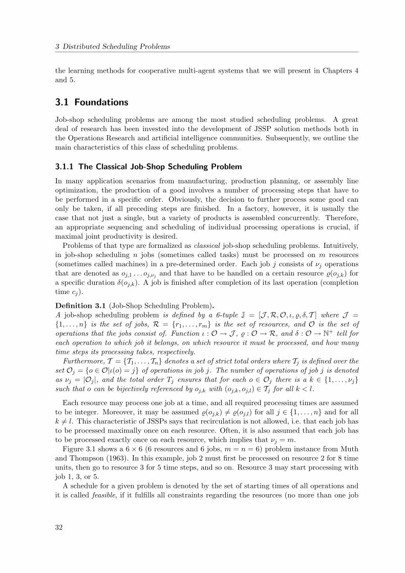
3 Distributed Scheduling Problems
the learning methods for cooperative multi-agent systems that we will present in Chapters 4and 5.
3.1 Foundations
Job-shop scheduling problems are among the most studied scheduling problems. A greatdeal of research has been invested into the development of JSSP solution methods both inthe Operations Research and artificial intelligence communities. Subsequently, we outline themain characteristics of this class of scheduling problems.
3.1.1 The Classical Job-Shop Scheduling Problem
In many application scenarios from manufacturing, production planning, or assembly lineoptimization, the production of a good involves a number of processing steps that have tobe performed in a specific order. Obviously, the decision to further process some good canonly be taken, if all preceding steps are finished. In a factory, however, it is usually thecase that not just a single, but a variety of products is assembled concurrently. Therefore,an appropriate sequencing and scheduling of individual processing operations is crucial, ifmaximal joint productivity is desired.
Problems of that type are formalized as classical job-shop scheduling problems. Intuitively,in job-shop scheduling n jobs (sometimes called tasks) must be processed on m resources(sometimes called machines) in a pre-determined order. Each job j consists of νj operationsthat are denoted as oj,1 . . . oj,νj and that have to be handled on a certain resource %(oj,k) fora specific duration δ(oj,k). A job is finished after completion of its last operation (completiontime cj).
Definition 3.1 (Job-Shop Scheduling Problem).A job-shop scheduling problem is defined by a 6-tuple J = [J ,R,O, ι, %, δ, T ] where J =1, . . . , n is the set of jobs, R = r1, . . . , rm is the set of resources, and O is the set ofoperations that the jobs consist of. Function ι : O → J , % : O → R, and δ : O → N+ tell foreach operation to which job it belongs, on which resource it must be processed, and how manytime steps its processing takes, respectively.
Furthermore, T = T1, . . . , Tn denotes a set of strict total orders where Tj is defined over theset Oj = o ∈ O|ι(o) = j of operations in job j. The number of operations of job j is denotedas νj = |Oj |, and the total order Tj ensures that for each o ∈ Oj there is a k ∈ 1, . . . , νjsuch that o can be bijectively referenced by oj,k with (oj,k, oj,l) ∈ Tj for all k < l.
Each resource may process one job at a time, and all required processing times are assumedto be integer. Moreover, it may be assumed %(oj,k) 6= %(oj,l) for all j ∈ 1, . . . , n and for allk 6= l. This characteristic of JSSPs says that recirculation is not allowed, i.e. that each job hasto be processed maximally once on each resource. Often, it is also assumed that each job hasto be processed exactly once on each resource, which implies that νj = m.
Figure 3.1 shows a 6× 6 (6 resources and 6 jobs, m = n = 6) problem instance from Muthand Thompson (1963). In this example, job 2 must first be processed on resource 2 for 8 timeunits, then go to resource 3 for 5 time steps, and so on. Resource 3 may start processing withjob 1, 3, or 5.
A schedule for a given problem is denoted by the set of starting times of all operations andit is called feasible, if it fulfills all constraints regarding the resources (no more than one job
32
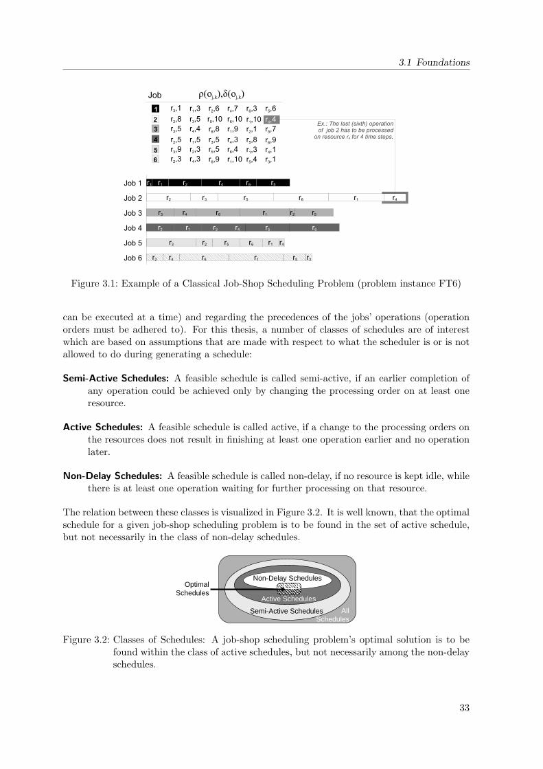
3.1 Foundations
Figure 3.1: Example of a Classical Job-Shop Scheduling Problem (problem instance FT6)
can be executed at a time) and regarding the precedences of the jobs’ operations (operationorders must be adhered to). For this thesis, a number of classes of schedules are of interestwhich are based on assumptions that are made with respect to what the scheduler is or is notallowed to do during generating a schedule:
Semi-Active Schedules: A feasible schedule is called semi-active, if an earlier completion ofany operation could be achieved only by changing the processing order on at least oneresource.
Active Schedules: A feasible schedule is called active, if a change to the processing orders onthe resources does not result in finishing at least one operation earlier and no operationlater.
Non-Delay Schedules: A feasible schedule is called non-delay, if no resource is kept idle, whilethere is at least one operation waiting for further processing on that resource.
The relation between these classes is visualized in Figure 3.2. It is well known, that the optimalschedule for a given job-shop scheduling problem is to be found in the set of active schedule,but not necessarily in the class of non-delay schedules.
Semi-Active Schedules AllSchedules
Active Schedules
Non-Delay SchedulesOptimal
Schedules
Figure 3.2: Classes of Schedules: A job-shop scheduling problem’s optimal solution is to befound within the class of active schedules, but not necessarily among the non-delayschedules.
33
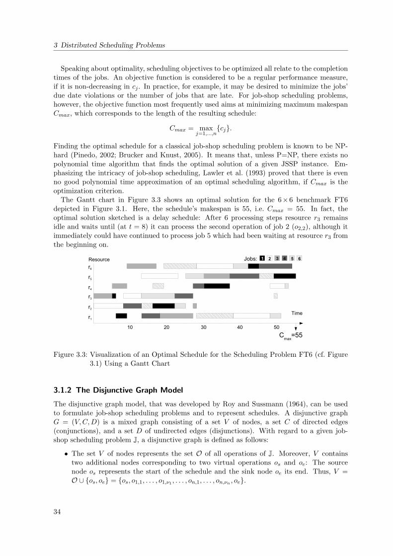
3 Distributed Scheduling Problems
Speaking about optimality, scheduling objectives to be optimized all relate to the completiontimes of the jobs. An objective function is considered to be a regular performance measure,if it is non-decreasing in cj . In practice, for example, it may be desired to minimize the jobs’due date violations or the number of jobs that are late. For job-shop scheduling problems,however, the objective function most frequently used aims at minimizing maximum makespanCmax, which corresponds to the length of the resulting schedule:
Cmax = maxj=1,...,n
cj.
Finding the optimal schedule for a classical job-shop scheduling problem is known to be NP-hard (Pinedo, 2002; Brucker and Knust, 2005). It means that, unless P=NP, there exists nopolynomial time algorithm that finds the optimal solution of a given JSSP instance. Em-phasizing the intricacy of job-shop scheduling, Lawler et al. (1993) proved that there is evenno good polynomial time approximation of an optimal scheduling algorithm, if Cmax is theoptimization criterion.
The Gantt chart in Figure 3.3 shows an optimal solution for the 6×6 benchmark FT6depicted in Figure 3.1. Here, the schedule’s makespan is 55, i.e. Cmax = 55. In fact, theoptimal solution sketched is a delay schedule: After 6 processing steps resource r3 remainsidle and waits until (at t = 8) it can process the second operation of job 2 (o2,2), although itimmediately could have continued to process job 5 which had been waiting at resource r3 fromthe beginning on.
Figure 3.3: Visualization of an Optimal Schedule for the Scheduling Problem FT6 (cf. Figure3.1) Using a Gantt Chart
3.1.2 The Disjunctive Graph Model
The disjunctive graph model, that was developed by Roy and Sussmann (1964), can be usedto formulate job-shop scheduling problems and to represent schedules. A disjunctive graphG = (V,C,D) is a mixed graph consisting of a set V of nodes, a set C of directed edges(conjunctions), and a set D of undirected edges (disjunctions). With regard to a given job-shop scheduling problem J, a disjunctive graph is defined as follows:
• The set V of nodes represents the set O of all operations of J. Moreover, V containstwo additional nodes corresponding to two virtual operations os and oe: The sourcenode os represents the start of the schedule and the sink node oe its end. Thus, V =O ∪ os, oe = os, o1,1, . . . , o1,ν1 , . . . , on,1, . . . , on,νn , oe.
34
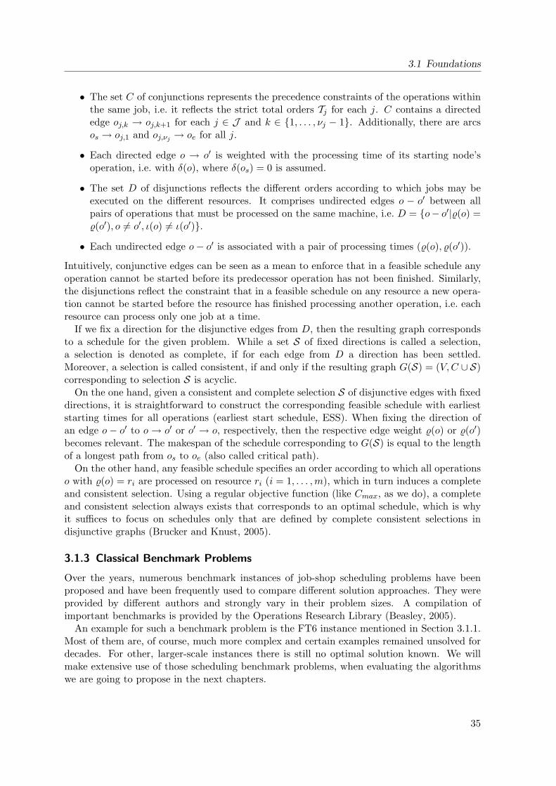
3.1 Foundations
• The set C of conjunctions represents the precedence constraints of the operations withinthe same job, i.e. it reflects the strict total orders Tj for each j. C contains a directededge oj,k → oj,k+1 for each j ∈ J and k ∈ 1, . . . , νj − 1. Additionally, there are arcsos → oj,1 and oj,νj → oe for all j.
• Each directed edge o → o′ is weighted with the processing time of its starting node’soperation, i.e. with δ(o), where δ(os) = 0 is assumed.
• The set D of disjunctions reflects the different orders according to which jobs may beexecuted on the different resources. It comprises undirected edges o − o′ between allpairs of operations that must be processed on the same machine, i.e. D = o− o′|%(o) =%(o′), o 6= o′, ι(o) 6= ι(o′).
• Each undirected edge o− o′ is associated with a pair of processing times (%(o), %(o′)).
Intuitively, conjunctive edges can be seen as a mean to enforce that in a feasible schedule anyoperation cannot be started before its predecessor operation has not been finished. Similarly,the disjunctions reflect the constraint that in a feasible schedule on any resource a new opera-tion cannot be started before the resource has finished processing another operation, i.e. eachresource can process only one job at a time.
If we fix a direction for the disjunctive edges from D, then the resulting graph correspondsto a schedule for the given problem. While a set S of fixed directions is called a selection,a selection is denoted as complete, if for each edge from D a direction has been settled.Moreover, a selection is called consistent, if and only if the resulting graph G(S) = (V,C ∪ S)corresponding to selection S is acyclic.
On the one hand, given a consistent and complete selection S of disjunctive edges with fixeddirections, it is straightforward to construct the corresponding feasible schedule with earlieststarting times for all operations (earliest start schedule, ESS). When fixing the direction ofan edge o− o′ to o → o′ or o′ → o, respectively, then the respective edge weight %(o) or %(o′)becomes relevant. The makespan of the schedule corresponding to G(S) is equal to the lengthof a longest path from os to oe (also called critical path).
On the other hand, any feasible schedule specifies an order according to which all operationso with %(o) = ri are processed on resource ri (i = 1, . . . ,m), which in turn induces a completeand consistent selection. Using a regular objective function (like Cmax, as we do), a completeand consistent selection always exists that corresponds to an optimal schedule, which is whyit suffices to focus on schedules only that are defined by complete consistent selections indisjunctive graphs (Brucker and Knust, 2005).
3.1.3 Classical Benchmark Problems
Over the years, numerous benchmark instances of job-shop scheduling problems have beenproposed and have been frequently used to compare different solution approaches. They wereprovided by different authors and strongly vary in their problem sizes. A compilation ofimportant benchmarks is provided by the Operations Research Library (Beasley, 2005).
An example for such a benchmark problem is the FT6 instance mentioned in Section 3.1.1.Most of them are, of course, much more complex and certain examples remained unsolved fordecades. For other, larger-scale instances there is still no optimal solution known. We willmake extensive use of those scheduling benchmark problems, when evaluating the algorithmswe are going to propose in the next chapters.
35
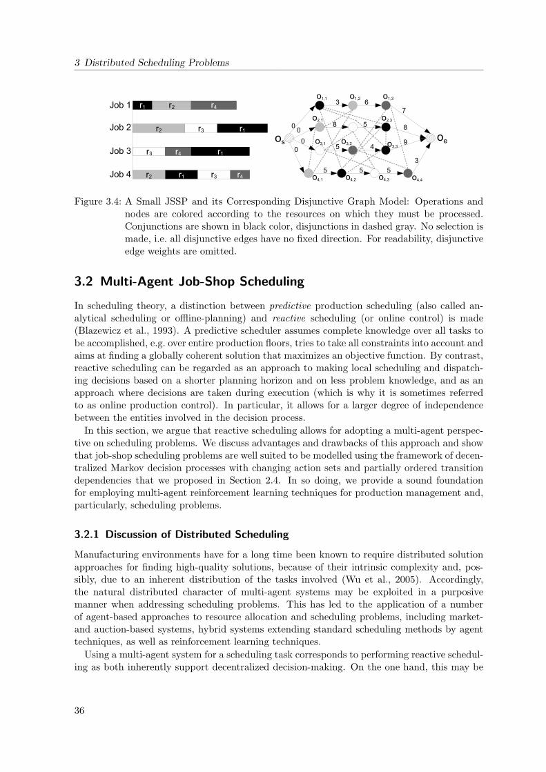
3 Distributed Scheduling Problems
Figure 3.4: A Small JSSP and its Corresponding Disjunctive Graph Model: Operations andnodes are colored according to the resources on which they must be processed.Conjunctions are shown in black color, disjunctions in dashed gray. No selection ismade, i.e. all disjunctive edges have no fixed direction. For readability, disjunctiveedge weights are omitted.
3.2 Multi-Agent Job-Shop Scheduling
In scheduling theory, a distinction between predictive production scheduling (also called an-alytical scheduling or offline-planning) and reactive scheduling (or online control) is made(Blazewicz et al., 1993). A predictive scheduler assumes complete knowledge over all tasks tobe accomplished, e.g. over entire production floors, tries to take all constraints into account andaims at finding a globally coherent solution that maximizes an objective function. By contrast,reactive scheduling can be regarded as an approach to making local scheduling and dispatch-ing decisions based on a shorter planning horizon and on less problem knowledge, and as anapproach where decisions are taken during execution (which is why it is sometimes referredto as online production control). In particular, it allows for a larger degree of independencebetween the entities involved in the decision process.
In this section, we argue that reactive scheduling allows for adopting a multi-agent perspec-tive on scheduling problems. We discuss advantages and drawbacks of this approach and showthat job-shop scheduling problems are well suited to be modelled using the framework of decen-tralized Markov decision processes with changing action sets and partially ordered transitiondependencies that we proposed in Section 2.4. In so doing, we provide a sound foundationfor employing multi-agent reinforcement learning techniques for production management and,particularly, scheduling problems.
3.2.1 Discussion of Distributed Scheduling
Manufacturing environments have for a long time been known to require distributed solutionapproaches for finding high-quality solutions, because of their intrinsic complexity and, pos-sibly, due to an inherent distribution of the tasks involved (Wu et al., 2005). Accordingly,the natural distributed character of multi-agent systems may be exploited in a purposivemanner when addressing scheduling problems. This has led to the application of a numberof agent-based approaches to resource allocation and scheduling problems, including market-and auction-based systems, hybrid systems extending standard scheduling methods by agenttechniques, as well as reinforcement learning techniques.
Using a multi-agent system for a scheduling task corresponds to performing reactive schedul-ing as both inherently support decentralized decision-making. On the one hand, this may be
36
3.2 Multi-Agent Job-Shop Scheduling
considered detrimental since a globally optimal solution cannot be yielded by doing reactivescheduling. By contrast, predictive schedulers – benefiting from full knowledge of the entirescheduling problem to be solved – typically attain the optimum. On the other hand, however,the list of potential merits of performing reactive scheduling using a multi-agent approach isnot to be underestimated:
• Reactive scheduling features the advantage of being able to react to unforeseen events(like a machine breakdown) appropriately without the need to do complete re-planning.
• Operations Research has to the bigger part focused on predictive scheduling and yieldednumerous excellent centralized algorithms capable of finding an optimal schedule in rea-sonable time. This works well for small and medium-sized JSSPs; for larger problemdimensions, however, computational complexity makes the application of centralized al-gorithms infeasible.
• The application of a centralized predictive scheduling algorithm in practice may requireenormous communication between the entities involved in the problem. Hence, lim-ited bandwidth or communication delays may render the use of a centralized approachimpossible.
• Many resource allocation or scheduling problems are intrinsically distributed in nature,meaning that there exists no central authority with all the necessary information toformulate and solve a centralized optimization problem. Stated from a practical point ofview, a centralized control cannot always be instantiated, which is why a decentralizedproblem interpretation using a multi-agent system may at times be of higher impact toreal-world applications.
• By combining partial solutions as provided by the agents involved for local problemsthey are facing, it may be feasible to find a more efficient solution for the global problem.Although in this way generally only near-optimal results will be obtained – as job-shopscheduling problems are known to be tightly interacting and non-decomposable (Liu andSycara, 1997) – that kind of divide and conquer strategy may be of high efficiency.
• Further advantages that can be claimed for taking a multi-agent approach to (practical)manufacturing and scheduling problems include increased flexibility, reduced costs, faulttolerance, and the fact that multi-agent systems may facilitate humans and agent-basedmachinery to work together as colleagues.
Baker (1998) survey in detail the utility of multi-agent systems for factory control, resourceallocation, and scheduling problems. While they name various different ways for utilizingagents for distributed production control (e.g. for deciding what and how much to produce, orwhen to release jobs into a factory), we subsequently focus on their use for deciding upon jobrouting and operation sequencing. In so doing, we associate to each of the m resources an agenti that locally decides which operation to process next. How this idea relates to DEC-MDPwith changing action sets is the subject of the next section.
3.2.2 Job-Shop Scheduling as Decentralized Markov Decision Process
Job-shop scheduling problems are well suited to be modelled using factored m-agent DEC-MDPs with changing action sets and partially ordered transition dependencies (see Definitions
37
3 Distributed Scheduling Problems
2.12 and 2.13). We reinforce this claim by showing how the components of a JSSP can beemployed to construct a corresponding DEC-MDP.
Factored World State The world state of a job-shop scheduling problem J (cf. Definition 3.1)can be factored: We assume that to each of the resources one agent i is associated thatobserves the local state at its resource and controls its behavior. Consequently, we haveas many agents as resources in the JSSP (|Ag| = |R| = m).
Local Full Observability The local state si of agent i, hence the situation of resource ri, isfully observable (thus, local observations and local states are identical). Additionally, thecomposition at all resources fully determines the global state of the scheduling problem.Therefore, the system is jointly observable, i.e. it is a DEC-MDP (cf. Definition 2.7).
Factored Actions Actions correspond to the starting of jobs’ operations (job dispatching). So,a local action of agent i reflects the decision to further process one particular job (moreprecisely, the next operation of that job) out of the set Ai ⊆ J of jobs currently waitingat ri.
Changing Action Sets If actions denote the dispatching of waiting jobs for further processing,then, apparently, the set of actions available to an agent varies over time, since the setof jobs waiting at a resource changes. While Ai ⊆ Ari denotes1 the currently availableactions for agent i, Ari is the set of all potentially executable actions for this agent.
Hence, Ari corresponds to the set of jobs j that contain an operation oj,k which must beprocessed on resource ri, i.e. %(oj,k) = i. Accordingly, it holds
Ar = ∪mi=1Ari = J . (3.1)
Furthermore, the local state si of agent i is fully described by the changing set of jobscurrently waiting at resource ri for further processing. Thus, si = Ai and Si = P(Ari ) asrequired by Definition 2.12.
Transition Dependencies DEC-MDPs with changing action sets and partially ordered tran-sition dependencies feature some structure according to which agents’ local action mayexert influence on the local state of other agents. After having finished an operation of ajob, this job is transferred to another resource, which corresponds to influencing anotheragent’s local state by extending that agent’s action set.
Dependency Functions The order of resources on which a job’s operations must be processedin a JSSP is given by the set of strict total orders T . These orders imply that, uponexecuting a local action by processing a job’s next operation, the local state of maximallyone further agent is influenced. Let α ∈ Ai (and so α ∈ J ) be the job whose currentoperation oα,k is processed by resource ri. Then, after having finished oα,k, the actionset Ai of agent i is adapted according to Ai := Ai \ α, whereas the action set of agenti′ = %(oα,k+1) is extended (Ai′ := Ai′ ∪ α).Therefore, we can define the dependency functions σi : Ari → Ag ∪ ∅ (cf. Definition2.13) for all agents i (and resource ri, respectively) as
σi(α) =
%(oα,k+1) if ∃k ∈ 1, . . . , να − 1 : %(oα,k) = i
∅ else(3.2)
1Recall that Ari = Ai \ α0 where α0 represents an idle action, cf. Definition 2.12.
38
3.2 Multi-Agent Job-Shop Scheduling
where k corresponds to the number of that operation within job α that has to be processedon resource ri, i.e. k such that %(oα,k) = i.
Dependency Graphs Given the no recirculation property (Section 3.1.1) and the definitionof σi (Equation 3.2), the directed graph Gα from Definition 2.13 is indeed acyclic andcontains only one directed path.
For job-shop scheduling problems with recirculation the definition of Gα must be slightlyextended; this depicts a rather technical change and is beyond our scope. For the norecirculation case we are addressing we prove the properties of Gα in the following propo-sition.
Proposition 1.Given a job-shop scheduling problem J without recirculation (cf. Definition 3.1) and the def-inition of the dependency functions σi (cf. Equation 3.2), the dependency graphs Gα for allα ∈ Ari = J (cf. Definition 2.13) are acyclic and contain only one directed path.
Proof. We show the acyclicity of Gα = (Ag,E) with
E = (j, σj(α))|j ∈ Ag, σj(α) 6= ∅ (3.3)
by contradiction. Assume there is a cycle of length c > 1 in Gα, consisting of nodes v1, . . . , vc ∈Ag and directed edges (v1, v2), . . . , (vc−1, vc), (vc, v1) ∈ E. Since (vx, vx+1) ∈ E and, hence,vx+1 = σvx(α) (for 1 ≤ x ≤ c − 1), and, consequently, σvx(α) 6= ∅, there exists a kx ∈1, . . . , να−1 such that %(oα,kx) = vx. Because also (vc, v1) ∈ E and, hence, v1 = σvc(α) and,in particular, σvc(α) 6= ∅, there also exists a kc ∈ 1, . . . , να − 1 such that %(oα,kc) = vc. So,we have %(oα,k1) = v1 as well as σvc(α) = %(oα,kc+1) = v1. By definition, ki < kj for all i < j,and kc > k1. Because of the latter there are two operations within job α (oα,k1 and oα,kc+1)that both must be processed on the same resource (on v1). This contradicts to the assumptionof a JSSP without recirculation from above.
Next, we prove that there exists only one directed path in Gα for every α ∈ Ari = J .Obviously, Equation 3.3 implies |E| ≤ |Ag| and
(i, j) ∈ E ⇔ ∃k ∈ 1, . . . , να − 1 : %(oα,k) = i.
By definition of σi (Equation 3.2), it also holds j = σi(α) = %(oα,k+1). Let k ∈ 1, . . . , να− 1and denote ik = %(oα,k). Then, it holds (ik, σik(α)) ∈ E and, again, by definition of σik
ek := (ik, σik(α)) = (%(oα,k), %(oα,k+1)) ∈ E.
Thus, the set of all ek ∈ E (for k ∈ 1, . . . , να) forms a path of length να.
Obviously, the ensemble of agents interacting with the DEC-MDP corresponding to a JSSPhave to strive for the same goal, namely for optimizing the objective function of the schedulingproblem. Consequently, a crucial precondition to enable the agents to learn to make sophis-ticated scheduling decisions is that the global reward function of the DEC-MDP coincideswith the overall objective of scheduling. If, for example, the goal of scheduling is to minimizetardiness (due date violations), then it may be appropriate to allot negative rewards, if one ormore jobs violate their deadlines. As indicated in Section 3.1.1, in this work our schedulingobjective is to minimize the makespan Cmax of the resulting schedule. From scheduling theory
39
3 Distributed Scheduling Problems
it is known that the makespan of a schedule is minimized, if as many resources as possibleare processing jobs concurrently and if as few as possible resources with queued jobs are inthe system: Usually, a high utilization of the resources implies a minimal makespan (Pinedo,2002), i.e. the minimal makespan of a non-delay schedule is achieved when the number of timesteps can be minimized during which jobs are waiting for processing at the resources’ queues.Therefore, the DEC-MDP’s reward function can be brought into alignment with the schedul-ing objective, if negative rewards are incurred when many jobs, that are waiting for furtherprocessing, are in the system and, hence, the overall utilization of the resources is poor.
We will more formally define suitable global reward functions in subsequent chapters whenwe develop corresponding learning algorithms for DEC-MDPs with changing action sets andpartially ordered transition dependencies. For the time being, we have demonstrated thatJSSPs can be easily cast as sequential decision problems using the subclass of general DEC-MDPs we have identified and analyzed in Section 2.4. Accordingly, we are in the position toexploit the benchmarking character of job-shop scheduling problems in a productive mannerfor the purpose of evaluating the performance of the reinforcement learning algorithms forDEC-MDPs we propose in Chapters 4 and 5.
3.3 Related Work on Solving Job-Shop Scheduling Problems
Job-shop scheduling has received an enormous amount of attention in the research literature.Both, complexity results and solution procedures have frequently been presented. As men-tioned in Section 3.2, research in production scheduling traditionally distinguishes predictiveand reactive solution approaches. Assuming complete knowledge about the entire schedulingproblem to be solved (thus about all jobs, their operations and belonging durations as well asabout the resources and which operations must be executed on which resource), and aimingat the achievement of global coherence in the process of job dispatching, Operations Researchhas brought about a variety of predictive scheduling algorithms that yield optimal solutionsfor individual problem instances – at least up to certain problem sizes, since the computationaleffort scales exponentially with problem size. By contrast, reactive scheduling approaches sup-port decentralized, local decision-making, which is beneficial when no centralized control canbe instantiated (e.g. when a factory’s resource does not know about the current workload atany other resource) or when quick responses to unexpected events are required.
Nearly all of the approaches that utilize ideas from research in artificial intelligence to solvescheduling problems belong to the realm of predictive scheduling. We will briefly review thatbody of work and give an outline of classical optimal solution methods and meta-heuristics. Asour formulation of JSSPs using decentralized Markov decision processes belongs to the realmof reactive scheduling we will pay special attention to related work from that field, including,most prominently, dispatching rules and further AI-based methods.
3.3.1 Optimal and Near-Optimal Solution Algorithms
Classical, predictive approaches to solving job-shop scheduling problems are mostly based upondisjunctive programming, i.e. on the disjunctive graph formulation of the problem presentedin Section 3.1.2. Based on this and on related graph formulations powerful algorithms havebeen proposed, such as branch-and-bound procedures (Carlier and Pinson, 1989; Applegateand Cook, 1991; Brucker et al., 1994) or tabu search approaches (Dell’Amico and Trubian,1993; Nowicki and Smutnicki, 1996, 2005).
40
3.3 Related Work on Solving Job-Shop Scheduling Problems
Moreover, there is a large number of local search procedures and meta-heuristics to solve job-shop scheduling problems near-optimally in a centralized manner. These include the shiftingbottleneck heuristic (Adams et al., 1988), beam search (Ow and Morton, 1988), simulated an-nealing (van Laarhoven et al., 1992), greedy randomized adaptive search procedures (GRASP,Binato et al., 2001), as well as squeaky wheel optimization (Joslin and Clements, 1999).
Given the disparity of centralized solution approaches from the distributed ones we arefocusing on in this work, we refer to Pinson (1995) for a more thorough overview of predictivesolution methods to JSSPs and to Vaessens et al. (1996) for scheduling methods employinglocal search.
3.3.2 Dispatching Priority Rules
In contrast to these predictive methods yielding to search for a single problem’s best solution,our problem interpretation as sequential decision problem utilizing decentralized Markov deci-sion processes belongs to the class of reactive scheduling techniques. When addressing reactivescheduling and providing a partial view on each of the processing resources only, dispatchingpriority rules represent the most notable reference.
Generally speaking, a dispatching algorithm decides how to use a factory’s resources onlyupon the resources’ availability, eventually upon the availability of other resources, and withrespect to the set of waiting jobs. In practice, dispatching rules have turned out to be highlyappropriate for situations where there is a wide or changing variety of products or whereadvance scheduling is difficult to implement.
Most dispatching rule research has been on deciding which job a resource will work on next.Basically, the rule computes a priority value for each of the waiting jobs based on some of itsparameters – such as jobs’ due dates, customer priorities, shortest remaining processing timesas well as any of dozens of different features characterizing a job – and selects the one which itconsiders to be the most urgent one. Panwalkar and Iskander (1977), Bhaskaran and Pinedo(1977), Wisner (1993), and Pinedo (2002) provide comprehensive reviews of dispatching rulesand their usage in industrial practice.
Dispatching priority rules (DPRs) can be classified along a number of dimensions. StaticDPRs, for example, make their decisions based solely on the waiting jobs’ and the respectiveresource’s data. By contrast, dynamic DPRs may change their behavior over time: If jobdeadline violations are to be minimized, the minimal slack rule, for instance, orders the waitingjobs with respect to their remaining processing times and their due dates. Hence, dependingon the current time and on the closeness of the jobs’ deadlines, this rule behaves differently.
Another way to classify DPRs considers whether a rule is a rather elementary or a compositeone, where the latter are composed of a number of the former ones. The distinction of DPRsmost relevant in the scope of this thesis focuses on the amount of information a rule basesits decisions on. A local DPR uses information only that pertain to the queue where a jobis waiting or to the resource on which that rule is deployed. Contrarily, global DPRs mayadditionally have access to information regarding other resources (such as the processing timeof a job on another resource) or even to the current state of other resources’ waiting queues.
The following list provides a selection of well-established dispatching priority rules that weare going to utilize for comparative reasons in the subsequent chapters. We provide briefcharacterizations and point out that this selection covers rather simple and more complexrules, as well as those that benefit from having granted access to more information than justthe local view onto their respective resource.
41
3 Distributed Scheduling Problems
Avoid Maximum Current Makespan (AMCC) Focusing on job-shop scheduling with block-ing and no-wait constraints, Mascis and Pacciarelli (2002) develop heuristic dispatchingrules, among them the powerful AMCC rule which benefits from having a global viewonto the entire plant, when making its dispatch decisions (global view rule). AMCC is aheuristic to avoid the maximum current Cmax based on the idea of repeatedly enlarginga consistent selection, given a general alternative graph representation of the schedulingproblem (Mascis and Pacciarelli, 2002).
First In First Out (FIFO) This well-known rule selects the job which has been waiting for thelongest time at the respective resource. The FIFO rule requires local view only.
Longest Processing Time (LPT) This rule iterates over all waiting jobs and executes thatjob whose next operation’s processing time is longest. To make this decision, again, onlya local view is required.
Random Dispatch Rule (RND) A random dispatcher always selects randomly one out of thecurrently waiting jobs.
Shortest Processing Time (SPT) This rule iterates over all waiting jobs and executes thatjob whose next operation’s processing time is shortest. The SPT rule is the counterpartto the LPT rule.
Shortest Queue for Next Operation (SQNO) This dispatching rule is allowed to retrieve in-formation regarding the situation on other resources (i.e. it is a global rule). Let resourceri be controlled by the SQNO rule. Then, for each job j out of the set of waiting jobsthis rule determines on which resource job j has to be processed after having been pro-cessed on ri. Then, the current status of the waiting queues of those potential successorresources is retrieved. Finally, the job is executed whose successor resource has currentlythe fewest jobs waiting.
DPRs are helpful, when attempting to find reasonably good schedules with regard to onespecific objective (such as makespan). They are easy to deploy and require minimal compu-tational effort. For large-scale or even real-life applications, however, DPRs are of limited useonly: Just sorting the jobs with respect to one or a few of their parameters may in generalnot lead to satisfying solutions. Composite rules, as mentioned above, depict an emendingextension for yielding a higher degree of generality, but their use and their composition is aknowledge-intensive task that requires a fair amount of prior knowledge about the schedulingproblem at hand. Having that in mind, some of the learning algorithms we are going to presentin subsequent chapters can be regarded as an approach to make agents learn highly complexcomposite dispatching priority rules that are adaptively customized.
3.3.3 Artificial Intelligence-Based Approaches
First of all, we stress that nearly all work on solving scheduling problems using approachesenhanced by AI methods assume full knowledge about the problem and, hence, perform pre-dictive scheduling. Many of these approaches depict intelligent search methods: Local searchprocedures employ the idea that a given solution, i.e. a given schedule, may be improved bymaking small changes. A neighborhood between possible solutions is assumed and solutionsare changed over and again which brings about better and better schedules. For example,
42
3.3 Related Work on Solving Job-Shop Scheduling Problems
there exists a substantial body of work that employs methods and ideas from evolutionarycomputing and genetic algorithms (e.g. Bean, 1994, Ombuki and Ventresca, 2004, or Gonzalezet al., 2008). Distributed AI-based approaches to solve job-shop scheduling problems are rare.Wu et al. (2005) point out that decentralized methods for resource allocation typically assumeself-interested agents and that market mechanisms (e.g. auctions) can be used to achieve thedesirable collective behavior among agents. While the focus of this line of research is on thedesign of multi-agent systems to resemble financial markets and on coalition formation, ourintention, when using JSSPs as application domain, is to study the learning capabilities of theagents.
Reinforcement Learning for Job-Shop Scheduling
Zhang and Dietterich (1995) were the first to apply a reinforcement learning approach fora special scheduling problem: They developed a repair-based scheduler that is trained usingthe temporal difference reinforcement learning algorithm and that starts with a critical-pathschedule and incrementally repairs constraint violations. Mahadevan et al. (1997) have pre-sented an average-reward reinforcement learning algorithm for the optimization of transferlines in production manufacturing which resembles a simplifying specialization of a schedul-ing problem. They show that the adaptive resources are able to effectively learn when theyhave to request maintenance, and that introducing a hierarchical decomposition of the learn-ing task is beneficial for obtaining superior results (Wang and Mahadevan, 1999). Anotherrepair-based approach relying on an intelligent computing algorithm is suggested by Zeng andSycara (1995) who make use of case-based reasoning and a simplified reinforcement learningalgorithm to achieve adaptation to changing optimization criteria.
Using our reactive approach to scheduling, the finally resulting schedule is not calculatedbeforehand, viz before execution time. Insofar, our reinforcement learning approach to job-shopscheduling, interpreting the problem as a sequential decision problem and using decentralizedMarkov decision processes, is rather different from these pieces of work mentioned. A reactive(closed-loop) perspective is also adopted by Schneider et al. (1998) who employ approximatedynamic programming algorithms to solve scheduling problems. However, they assume a singlelearning agent that fully observes the state. Similarly, Aydin and Oztemel (2000) developedan extended version of Q learning, which they entitle Q-III learning and embed into an agent-based system which performs scheduling in a centralized way.
Independently learning agents for a reactive scheduling setting were also investigated byCsaji and Monostori (2004). They interpret JSSPs as a market-based production controlsystem, attach agents to resources as well as to jobs, allow them to interact with each otherusing biddings and contracts, and to optimize their bidding behavior using temporal differencereinforcement learning. In later work, these authors turned to centralized solution approachesfor job-shop scheduling problems using a combination of Q learning, rollout algorithms, andsupport vector regression for value function approximation (Csaji and Monostori, 2006) plusa technique for parallelizing the learning algorithm (Csaji and Monostori, 2008).
While the references mentioned so far are barely or only loosely related to our approach,in using JSSPs as challenging application domain for investigating the performance of coop-erative learning multi-agent systems, we have drawn a lot of inspiration from the work byRiedmiller and Riedmiller (1999) who employed neural reinforcement learning in conjunctionwith multi-layer perceptrons for Q function approximation to learn local dispatching policies.The investigations we present in Chapter 5 are highly related to their work and depict a direct
43

3 Distributed Scheduling Problems
extension of their approach.Before, however, we are going to explore value function-based reinforcement learning ap-
proaches for cooperative multi-agent systems and for the application domain of job-shopscheduling, we analyze the use of policy search-based reinforcement learning techniques inthe next chapter.
44
4 Policy Search-Based Solution Approaches
In Chapter 2 we have seen that the jump from one to many agents interacting with theenvironment brings about a significant increase in complexity, when aiming at the acquisitionof a joint policy that yields global welfare. This kind of problem aggravation is mainly causedby the fact that each single agent is unaware about other agents’ local states, their beliefs, andthe policies they are pursuing.
In Section 2.4, we treaded a path of counteracting that rise in complexity by identify-ing a specific subclass of general distributed decision problems, viz the class of decentralizedDEC-MDPs with changing action sets and partially ordered transition dependencies, which isprovably easier to solve (NP- instead of NEXP-hard). While this is a positive result (sinceNP(NEXP), solving NP-hard problems is far from being easy: Except for the case that NP=P,which is a hitherto unanswered question, there exists no algorithm that is capable of solvingNP problems in time bounded polynomially in the problem’s size.
Consequently, in this as well as in the next chapter we are going to investigate alterna-tive approaches to tackling decentralized decision problems. Instead of attempting to findan optimal solution, i.e. an optimal joint policy, for a given multi-agent problem, we strivefor acquiring approximate and potentially near-optimal solutions in feasible time using rein-forcement learning. While we advocate Chapter 5 to the value function-based approach toreinforcement learning, in the chapter at hand we develop two different policy search-basedreinforcement learning methods for cooperative multi-agent systems, analyze their theoreticalproperties, and investigate them empirically.
After some foundations and motivation for the use of policy search reinforcement learning(Section 4.1), we propose a direct policy search technique, dubbed joint equilibrium policysearch (JEPS, Section 4.2), and a gradient-descent policy search approach (GDPS, Section 4.3)for the subclass of DEC-MDPs we are addressing. The performance of both of these methodsin terms of quickly acquiring high-quality joint policies will be analyzed for numerous intricatejob-shop scheduling benchmarks that are interpreted as DEC-MDPs with changing action setsas described in Section 3.2.2. We finish this chapter with a discussion of the advantages anddrawbacks of policy search reinforcement learning, leading us to the alternative value function-based approach that will, as mentioned, move into our focus in the subsequent chapter.
4.1 Foundations
According to Sutton and Barto (1998), reinforcement learning is a problem description ratherthan a specific solution method. The policy search-based approach to the reinforcement learn-ing problem draws quite some of its motivation from a simplicity argument: The goal oflearning is to solve the learning problem by finding the best policy of action, irrespectiveof the deeper structure of the experience gathered during interacting with the environment.Thus, if it is possible for the learning process to directly yield solutions without performing anintermediate system identification process (e.g. by estimating the transition or reward model),
45
4 Policy Search-Based Solution Approaches
then robust and high-quality learning results can be obtained even when the underlying systemis too complex to estimate (Strens and Moore, 2001).
In this spirit and with regard to the actor-critic architecture introduced in Section 2.1.3, pol-icy search methods correspond to actor-focused techniques which basically rely on an explicitrepresentation of an actor, i.e. on an explicit representation of the policy.
Policy search represents an attractive approach to reinforcement learning problems for var-ious reasons:
1. As outlined in Section 2.1.4, the complexity of the search through the space of possiblepolicies can be heavily reduced, if the search is restricted to a relevant subspace whichcan be defined through the exploitation of possibly available problem knowledge.
2. Besides this, it is important to stress that policy search reinforcement learning focuses onthe evaluation of policies as a whole, assessing their performance over, typically, largersequences of action choices. This is one of the reasons, why policy search approacheshave been found useful for learning under partial observability (Meuleau et al., 1999).Logically, this merit also applies to multi-agent reinforcement learning within DEC-MDPs where each agent has only its local and, hence, incomplete perception of theworld state (Baird and Moore, 1999).
3. By definition, policy search algorithms are model-free techniques, not requiring knowl-edge about the transition and reward functions of the underlying Markov decision pro-cess. While model-based methods presume to possess or estimate a model of the environ-ment and compute or infer a policy with the help of this model, policy search algorithmsare facilitated to attempt for finding a good policy directly.
4. Policy search methods have sometimes been reported to outperform traditional valuefunction-based temporal difference reinforcement learning algorithms for several tasks(Taylor et al., 2006; Stanley and Miikkulainen, 2002).
4.1.1 Policy Performance
Policy search methods search directly in the space P of policies without learning value functions.This can be a highly effective approach, particularly if a fair amount of problem knowledgeregarding the learning task at hand is available. The exploitation of background knowledge asa mean to guide machine learning algorithms and to restrict search processes is well-known andfrequently applied approach (Gabel and Stahl, 2004). Concerning policy search reinforcementlearning, the incorporation of task knowledge may take shape as parameterizing a policy using a(small) vector θ of real-valued parameters: By defining the domains of these parameters as wellas how the parameter vector influences action choices, and moreover interpreting the searchprocess as a search over those parameters, a tremendous reduction of the search complexitycan be achieved. For decentralized Markov decision processes with changing action sets andpartially ordered transition dependencies, additional prior knowledge may enhance the search,for example, by exploiting the fact that each agent may execute each action α ∈ Ari only once(cf. Lemma 1).
Central to policy optimization using policy search-based reinforcement learning is the notionof the quality or performance J(πθ) of a policy πθ that is defined through its parameters θ.
46
4.1 Foundations
Definition 4.1 (Policy Performance).Given a distribution over a set S0 ⊂ S of starting states, the performance of a policy πθis defined as the expected value of the return R0, which is defined as the discounted sum ofimmediate rewards r, that is to be expected when starting from a state s0 ∈ S0 and pursuingπθ thereafter until reaching a final state after D decision stages:
J(πθ) = E[R0|s0 ∈ S0, πθ] = E[D∑k=0
γkr(k)|πθ] = limN→∞
1N
N∑l=1
R(l) (4.1)
where R(l) refers to the return obtained during the lth episode.
From Equation 4.1 it is obvious, that J(πθ) is closely related to the definition of the valueV π(s) of a state according to Equation 2.2, if we consider E[V π(s)|s ∈ S0]. Moreover, forproblems with a single starting state, i.e. S0 = s0, it holds J(πθ) = V π(s0). Given Definition4.1 it follows immediately, that the goal of a policy search approach is to improve J(πθ) byadapting θ in a purposive and efficient manner.
4.1.2 Multi-Agent Policy Search Reinforcement Learning
The core idea of policy search-based reinforcement learning is to directly adapt the policy tobe learned with respect to its performance, while the key point of cooperative multi-agentreinforcement learning is to have independent agents that try to improve their local policieswith respect to a common goal. Algorithm 4.1 provides a straightforward implementation of aprocedure that is tailored for policy search reinforcement learning and that lets a single agentinteract with the environment (in our case, a DEC-MDP) and improve its policy independently.Note that this algorithm is to be executed in parallel by each agent involved; we here describeit from a single agent’s perspective only.
Until some external stop signal indicates the end of the entire learning process, agent i alter-nates between fully observing its local state, choosing actions, and obtaining global immediaterewards. On the occasion of having finished a single episode, as indicated by having enteredthe terminal state sf , the agent calls a policy update algorithm (line 10) whose task is topurposively process the experience collected during the recent episode. In the following twosubsections we develop and analyze different variants of such update algorithms. Thus, Algo-rithm 4.1 realizes a rather generic procedure for performing policy search-based reinforcementlearning using decentralized control. Basically, it realizes the interaction of a single agent(agent i) with the DEC-MDP with changing action sets at hand and delegates the task oflearning to the respective policy update methods.
We note that variable d in Algorithm 4.1 does not necessarily have to correspond to timesteps, but merely represents a counter of decision steps experienced by agent i. Thus, thisalgorithm can also handle environments with temporally extended actions, i.e. where the exe-cution of a local action α lasts longer than one time step. For this to happen, the execution ofα in line 14 would correspond to a blocking function call and the global reward to be received(line 6) must be a collection of time step-based rewards accrued during the execution of α.
An important data structure utilized by Algorithm 4.1 is that of an experience sequence hthat is realized as a simple list. It corresponds to the processing of a single episode startingfrom some initial state and ending upon having reached the terminal state sf where no moreactions are available for any of the agents. Because we will use the notion of an experiencesequence repeatedly below, we provide a formal definition.
47
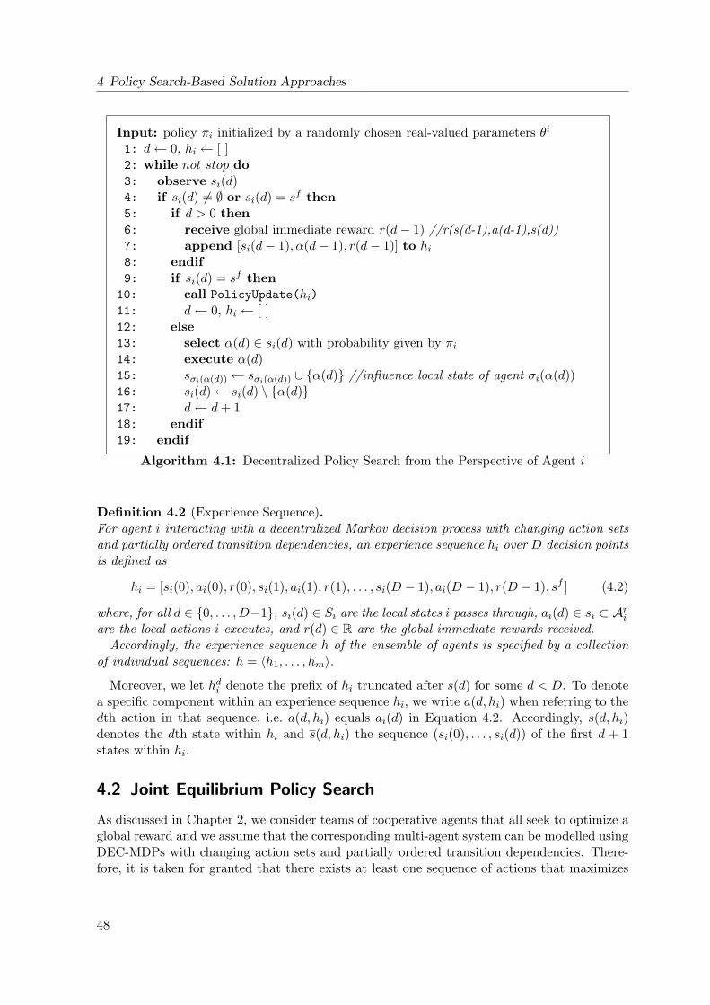
4 Policy Search-Based Solution Approaches
Input: policy πi initialized by a randomly chosen real-valued parameters θi
1: d← 0, hi ← [ ]2: while not stop do3: observe si(d)4: if si(d) 6= ∅ or si(d) = sf then5: if d > 0 then6: receive global immediate reward r(d− 1) //r(s(d-1),a(d-1),s(d))7: append [si(d− 1), α(d− 1), r(d− 1)] to hi8: endif9: if si(d) = sf then
10: call PolicyUpdate(hi)11: d← 0, hi ← [ ]12: else13: select α(d) ∈ si(d) with probability given by πi14: execute α(d)15: sσi(α(d)) ← sσi(α(d)) ∪ α(d) //influence local state of agent σi(α(d))16: si(d)← si(d) \ α(d)17: d← d+ 118: endif19: endif
Algorithm 4.1: Decentralized Policy Search from the Perspective of Agent i
Definition 4.2 (Experience Sequence).For agent i interacting with a decentralized Markov decision process with changing action setsand partially ordered transition dependencies, an experience sequence hi over D decision pointsis defined as
hi = [si(0), ai(0), r(0), si(1), ai(1), r(1), . . . , si(D − 1), ai(D − 1), r(D − 1), sf ] (4.2)
where, for all d ∈ 0, . . . , D−1, si(d) ∈ Si are the local states i passes through, ai(d) ∈ si ⊂ Ariare the local actions i executes, and r(d) ∈ R are the global immediate rewards received.
Accordingly, the experience sequence h of the ensemble of agents is specified by a collectionof individual sequences: h = 〈h1, . . . , hm〉.
Moreover, we let hdi denote the prefix of hi truncated after s(d) for some d < D. To denotea specific component within an experience sequence hi, we write a(d, hi) when referring to thedth action in that sequence, i.e. a(d, hi) equals ai(d) in Equation 4.2. Accordingly, s(d, hi)denotes the dth state within hi and s(d, hi) the sequence (si(0), . . . , si(d)) of the first d + 1states within hi.
4.2 Joint Equilibrium Policy Search
As discussed in Chapter 2, we consider teams of cooperative agents that all seek to optimize aglobal reward and we assume that the corresponding multi-agent system can be modelled usingDEC-MDPs with changing action sets and partially ordered transition dependencies. There-fore, it is taken for granted that there exists at least one sequence of actions that maximizes
48
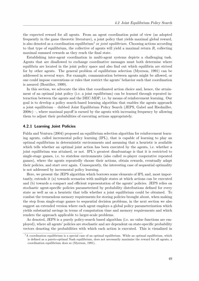
4.2 Joint Equilibrium Policy Search
the expected reward for all agents. From an agent coordination point of view (as adoptedfrequently in the game theoretic literature), a joint policy that yields maximal global reward,is also denoted as a coordination equilibrium1 or joint equilibrium. Choosing actions accordingto that type of equilibrium, the collective of agents will yield a maximal return R, collectingmaximal summed rewards as they reach the final state.
Establishing inter-agent coordination in multi-agent systems depicts a challenging task.Agents that are disallowed to exchange coordinative messages must both determine whereequilibria are located in the joint policy space and also find out which equilibria are strivedfor by other agents. The general problem of equilibrium selection (Myerson, 1991) can beaddressed in several ways. For example, communication between agents might be allowed, orone could impose conventions or rules that restrict the agents’ behavior such that coordinationis assured (Boutilier, 1999).
In this section, we advocate the idea that coordinated action choice and, hence, the attain-ment of an optimal joint policy (i.e. a joint equilibrium) can be learned through repeated in-teraction between the agents and the DEC-MDP, i.e. by means of reinforcement learning. Ourgoal is to develop a policy search-based learning algorithm that enables the agents approacha joint equilibrium – dubbed Joint Equilibrium Policy Search (JEPS, Gabel and Riedmiller,2008c) –, where maximal payoff is earned by the agents with increasing frequency by allowingthem to adjust their probabilities of executing actions appropriately.
4.2.1 Learning Joint Policies
Fulda and Ventura (2004) proposed an equilibrium selection algorithm for reinforcement learn-ing agents, called incremental policy learning (IPL), that is capable of learning to play anoptimal equilibrium in deterministic environments and assuming that a heuristic is availablewhich tells whether an optimal joint action has been executed by the agents, i.e. whether ajoint equilibrium was attained, or not. IPL’s greatest disadvantage is that it is restricted tosingle-stage games, i.e. to stateless environments (also called m-player cooperative repeatedgames), where the agents repeatedly choose their actions, obtain rewards, eventually adapttheir policies, and start over again. Consequently, the interesting case of sequential optimalityis not addressed by incremental policy learning.
Here, we present the JEPS algorithm which borrows some elements of IPL and, most impor-tantly, extends it (a) towards scenarios with multiple states at which actions can be executedand (b) towards a compact and efficient representation of the agents’ policies. JEPS relies onstochastic agent-specific policies parameterized by probability distributions defined for everystate as well as on a heuristic that tells whether a joint equilibrium could be obtained. Tocombat the tremendous memory requirements for storing policies brought about, when makingthe step from single-stage games to sequential decision problems, in the next section we alsosuggest an extended version where each agent employs a global policy parameterization whichyields substantial savings in terms of computation time and memory requirements and whichrenders the approach applicable to larger-scale problems.
As denoted, JEPS is a purely policy-search based algorithm (i.e. no value functions are em-ployed), where all agents’ policies are stochastic and are dependent on state-specific probabilityvectors denoting the probabilities with which each action is executed. This is visualized in
1A coordination equilibrium is a special case of an optimal equilibrium. While an optimal equilibrium, whichis defined as a pareto-optimal Nash equilibrium, does not necessarily maximize the reward for all agents, acoordination equilibrium does so (Myerson, 1991).
49
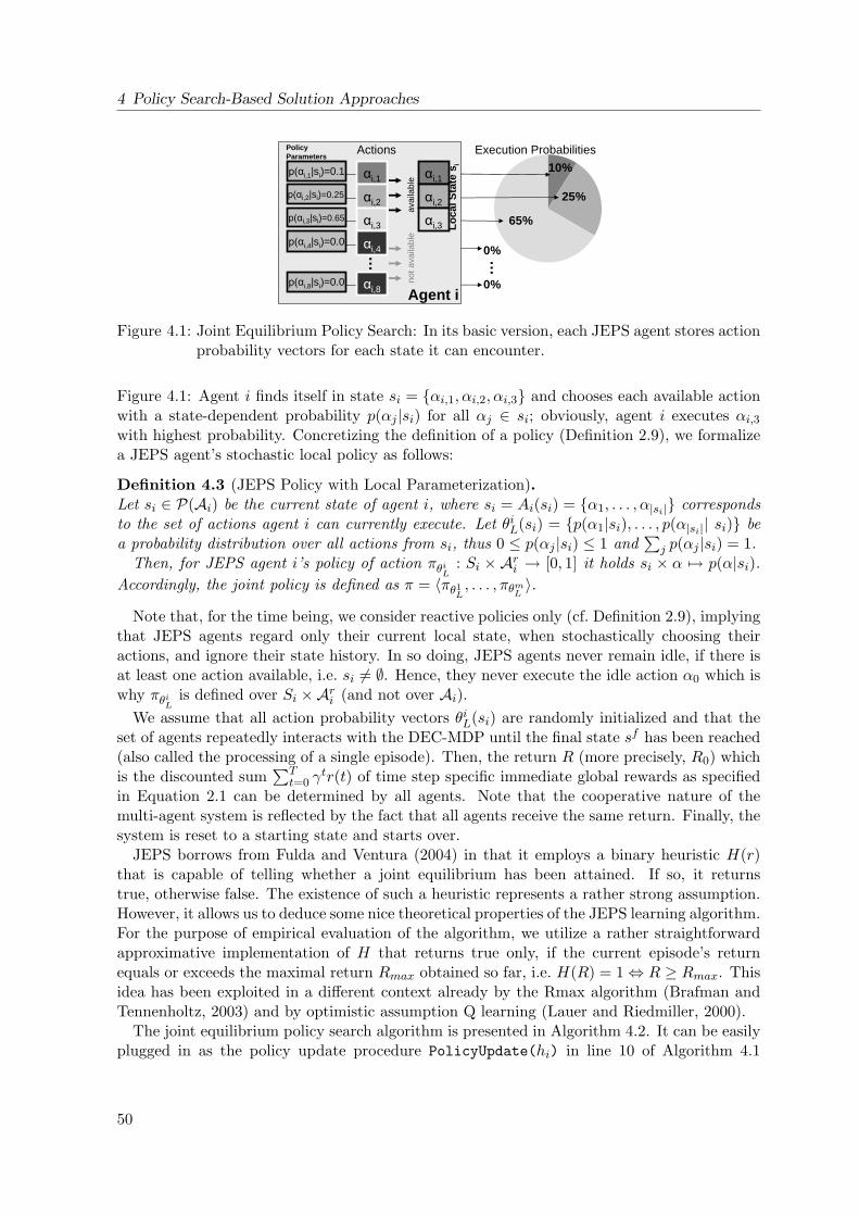
4 Policy Search-Based Solution Approaches
Agent i
Actions
avai
labl
e αi,1
αi,2
Loca
lSta
te s
i
αi,3
nota
vaila
ble
…
PolicyParameters
p(αi,1|si)=0.1
p(αi,2|si)=0.25
p(αi,3|si)=0.65
p(αi,8|si)=0.0
p(αi,4|si)=0.0
αi,1
αi,2
αi,3
αi,8
αi,4
10%
25%
65%
0%…
0%
Execution Probabilities
Figure 4.1: Joint Equilibrium Policy Search: In its basic version, each JEPS agent stores actionprobability vectors for each state it can encounter.
Figure 4.1: Agent i finds itself in state si = αi,1, αi,2, αi,3 and chooses each available actionwith a state-dependent probability p(αj |si) for all αj ∈ si; obviously, agent i executes αi,3with highest probability. Concretizing the definition of a policy (Definition 2.9), we formalizea JEPS agent’s stochastic local policy as follows:
Definition 4.3 (JEPS Policy with Local Parameterization).Let si ∈ P(Ai) be the current state of agent i, where si = Ai(si) = α1, . . . , α|si| correspondsto the set of actions agent i can currently execute. Let θiL(si) = p(α1|si), . . . , p(α|si|| si) bea probability distribution over all actions from si, thus 0 ≤ p(αj |si) ≤ 1 and
∑j p(αj |si) = 1.
Then, for JEPS agent i’s policy of action πθiL: Si × Ari → [0, 1] it holds si × α 7→ p(α|si).
Accordingly, the joint policy is defined as π = 〈πθ1L , . . . , πθmL 〉.
Note that, for the time being, we consider reactive policies only (cf. Definition 2.9), implyingthat JEPS agents regard only their current local state, when stochastically choosing theiractions, and ignore their state history. In so doing, JEPS agents never remain idle, if there isat least one action available, i.e. si 6= ∅. Hence, they never execute the idle action α0 which iswhy πθiL is defined over Si ×Ari (and not over Ai).
We assume that all action probability vectors θiL(si) are randomly initialized and that theset of agents repeatedly interacts with the DEC-MDP until the final state sf has been reached(also called the processing of a single episode). Then, the return R (more precisely, R0) whichis the discounted sum
∑Tt=0 γ
tr(t) of time step specific immediate global rewards as specifiedin Equation 2.1 can be determined by all agents. Note that the cooperative nature of themulti-agent system is reflected by the fact that all agents receive the same return. Finally, thesystem is reset to a starting state and starts over.
JEPS borrows from Fulda and Ventura (2004) in that it employs a binary heuristic H(r)that is capable of telling whether a joint equilibrium has been attained. If so, it returnstrue, otherwise false. The existence of such a heuristic represents a rather strong assumption.However, it allows us to deduce some nice theoretical properties of the JEPS learning algorithm.For the purpose of empirical evaluation of the algorithm, we utilize a rather straightforwardapproximative implementation of H that returns true only, if the current episode’s returnequals or exceeds the maximal return Rmax obtained so far, i.e. H(R) = 1⇔ R ≥ Rmax. Thisidea has been exploited in a different context already by the Rmax algorithm (Brafman andTennenholtz, 2003) and by optimistic assumption Q learning (Lauer and Riedmiller, 2000).
The joint equilibrium policy search algorithm is presented in Algorithm 4.2. It can be easilyplugged in as the policy update procedure PolicyUpdate(hi) in line 10 of Algorithm 4.1
50
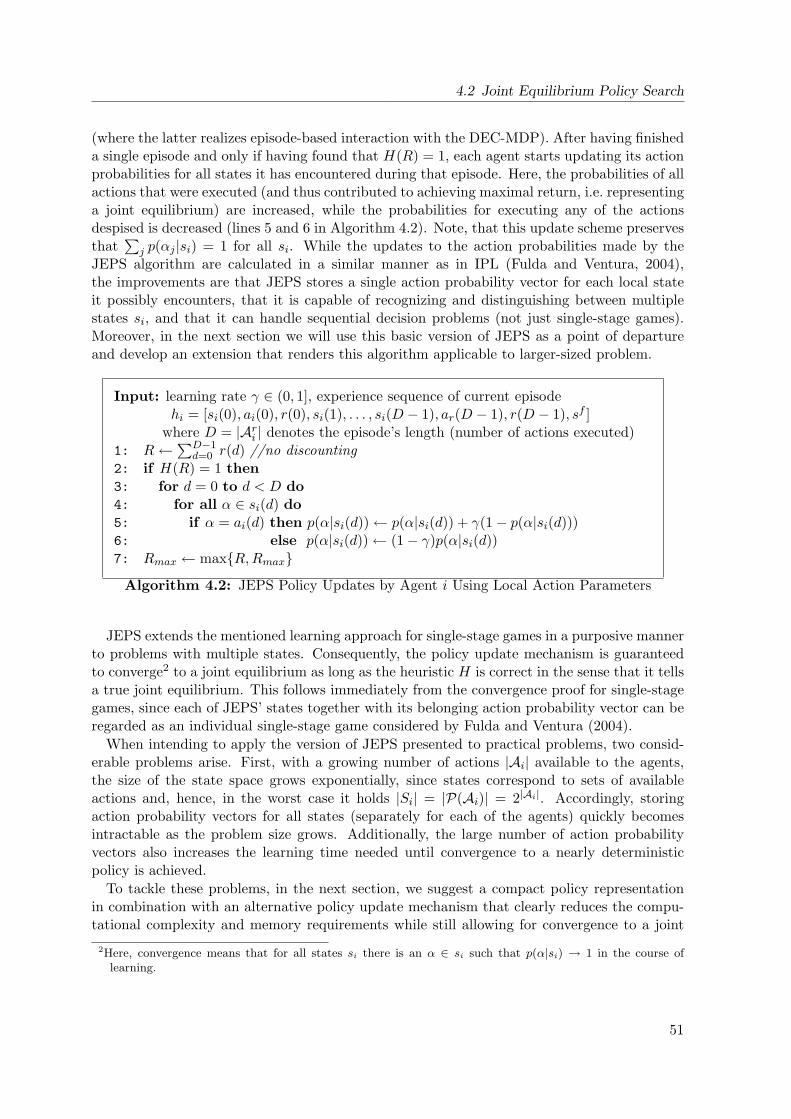
4.2 Joint Equilibrium Policy Search
(where the latter realizes episode-based interaction with the DEC-MDP). After having finisheda single episode and only if having found that H(R) = 1, each agent starts updating its actionprobabilities for all states it has encountered during that episode. Here, the probabilities of allactions that were executed (and thus contributed to achieving maximal return, i.e. representinga joint equilibrium) are increased, while the probabilities for executing any of the actionsdespised is decreased (lines 5 and 6 in Algorithm 4.2). Note, that this update scheme preservesthat
∑j p(αj |si) = 1 for all si. While the updates to the action probabilities made by the
JEPS algorithm are calculated in a similar manner as in IPL (Fulda and Ventura, 2004),the improvements are that JEPS stores a single action probability vector for each local stateit possibly encounters, that it is capable of recognizing and distinguishing between multiplestates si, and that it can handle sequential decision problems (not just single-stage games).Moreover, in the next section we will use this basic version of JEPS as a point of departureand develop an extension that renders this algorithm applicable to larger-sized problem.
Input: learning rate γ ∈ (0, 1], experience sequence of current episodehi = [si(0), ai(0), r(0), si(1), . . . , si(D − 1), ar(D − 1), r(D − 1), sf ]
where D = |Ari | denotes the episode’s length (number of actions executed)1: R←
∑D−1d=0 r(d) //no discounting
2: if H(R) = 1 then3: for d = 0 to d < D do4: for all α ∈ si(d) do5: if α = ai(d) then p(α|si(d))← p(α|si(d)) + γ(1− p(α|si(d)))6: else p(α|si(d))← (1− γ)p(α|si(d))7: Rmax ← maxR,Rmax
Algorithm 4.2: JEPS Policy Updates by Agent i Using Local Action Parameters
JEPS extends the mentioned learning approach for single-stage games in a purposive mannerto problems with multiple states. Consequently, the policy update mechanism is guaranteedto converge2 to a joint equilibrium as long as the heuristic H is correct in the sense that it tellsa true joint equilibrium. This follows immediately from the convergence proof for single-stagegames, since each of JEPS’ states together with its belonging action probability vector can beregarded as an individual single-stage game considered by Fulda and Ventura (2004).
When intending to apply the version of JEPS presented to practical problems, two consid-erable problems arise. First, with a growing number of actions |Ai| available to the agents,the size of the state space grows exponentially, since states correspond to sets of availableactions and, hence, in the worst case it holds |Si| = |P(Ai)| = 2|Ai|. Accordingly, storingaction probability vectors for all states (separately for each of the agents) quickly becomesintractable as the problem size grows. Additionally, the large number of action probabilityvectors also increases the learning time needed until convergence to a nearly deterministicpolicy is achieved.
To tackle these problems, in the next section, we suggest a compact policy representationin combination with an alternative policy update mechanism that clearly reduces the compu-tational complexity and memory requirements while still allowing for convergence to a joint
2Here, convergence means that for all states si there is an α ∈ si such that p(α|si) → 1 in the course oflearning.
51
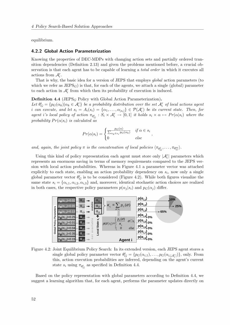
4 Policy Search-Based Solution Approaches
equilibrium.
4.2.2 Global Action Parameterization
Knowing the properties of DEC-MDPs with changing action sets and partially ordered tran-sition dependencies (Definition 2.13) and given the problems mentioned before, a crucial ob-servation is that each agent has to be capable of learning a total order in which it executes allactions from Ari .
That is why, the basic idea for a version of JEPS that employs global action parameters (towhich we refer as JEPSG) is that, for each of the agents, we attach a single (global) parameterto each action in Ari from which then its probability of execution is induced.
Definition 4.4 (JEPSG Policy with Global Action Parameterization).Let θiG = pG(αk)|αk ∈ Ari be a probability distribution over the set Ari of local actions agenti can execute, and let si = Ai(si) = α1, . . . , α|si| ∈ P(Ari ) be its current state. Then, foragent i’s local policy of action πθiG
: Si × Ari → [0, 1] it holds si × α 7→ Pr(α|si) where theprobability Pr(α|si) is calculated as
Pr(α|si) =
pG(α)Pαk∈si
pG(αk) if α ∈ si0 else
,
and, again, the joint policy π is the concatenation of local policies 〈πθ1G , . . . , πθmG 〉.
Using this kind of policy representation each agent must store only |Ari | parameters whichrepresents an enormous saving in terms of memory requirements compared to the JEPS ver-sion with local action probabilities. Whereas in Figure 4.1 a parameter vector was attachedexplicitly to each state, enabling an action probability dependency on si, now only a singleglobal parameter vector θiG is to be considered (Figure 4.2). While both figures visualize thesame state si = αi,1, αi,2, αi,3 and, moreover, identical stochastic action choices are realizedin both cases, the respective policy parameters p(αj |si) and pG(αj) differ.
∈=
else
sp
sp is
G
i i
0
)()|(
ακ
αα
Agent i
αi1
αi2
Lo
calS
tate
si
αi3
Glo
bal
Po
licy
Par
amet
ers
pGGGG(α1)=0.02
pGGGG(α2)=0.05
pGGGG(α3)=0.13
pGGGG(αi,8)=0.15
pGGGG(αi,4)=0.25
pGGGG(αi,5)=0.01
pGGGG(αi,6)=0.04
pGGGG(αi,7)=0.35
αi,1
αi,2
αi,8
αi,4
αi,7
αi,6
αi,5
avai
labl
en
o t
a v
a i
l a b
l e
∑∈
=i
is
Gs pα
ακ )(
10%
25%
65%
0%
p(αi,3)
p(αi,2)
p(αi,1)
p(αi,4)
p(αi,7)
p(αi,6)
p(αi,5)
p(αi,8)
0%
0%
0%
0%
pGGGG(αi,1)=0.02
pGGGG(αi,2)=0.05
pGGGG(αi,3)=0.13 αi,3
Figure 4.2: Joint Equilibrium Policy Search: In its extended version, each JEPS agent stores asingle global policy parameter vector θiG = pG(αi,1), . . . , pG(αi,|Ari |), only. Fromthis, action execution probabilities are inferred, depending on the agent’s currentstate si using πθiG as specified in Definition 4.4.
Based on the policy representation with global parameters according to Definition 4.4, wesuggest a learning algorithm that, for each agent, performs the parameter updates directly on
52
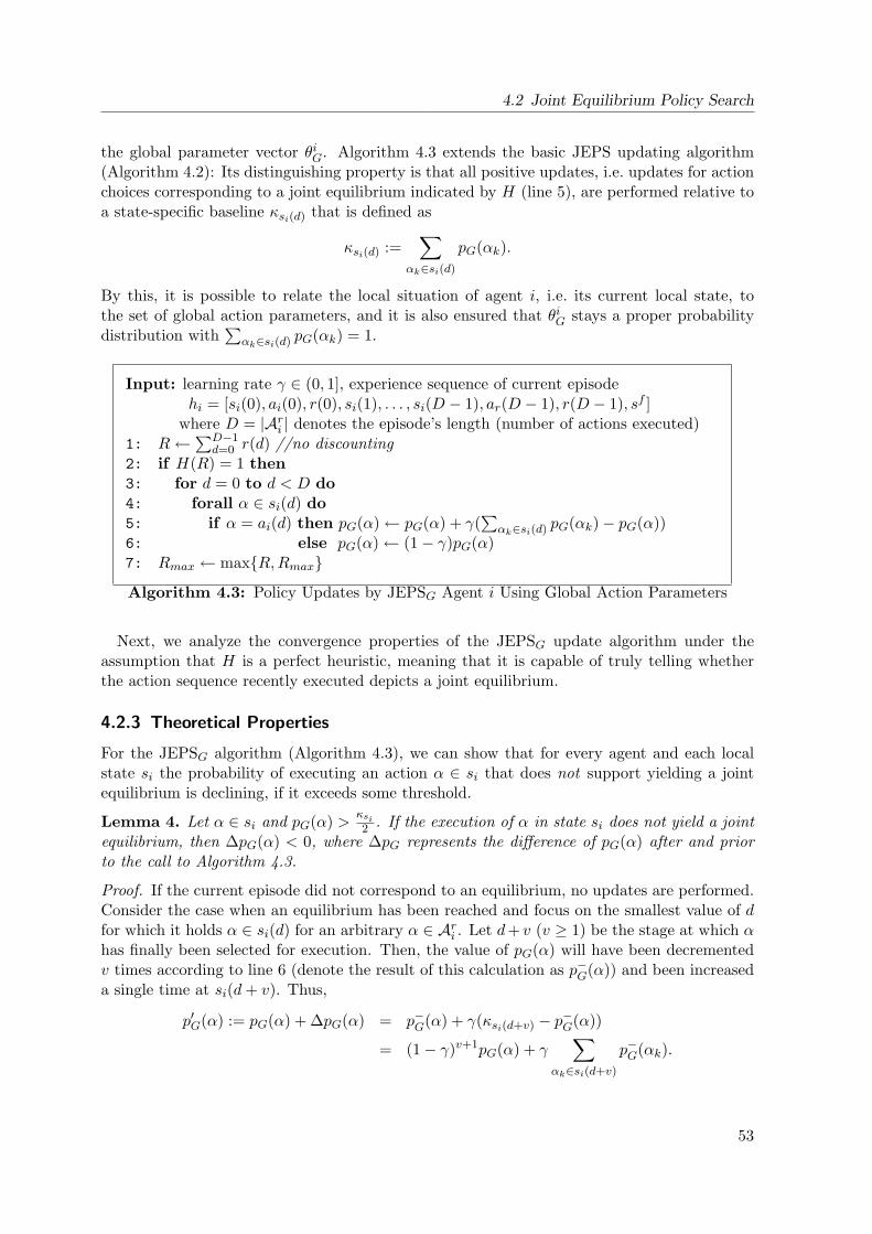
4.2 Joint Equilibrium Policy Search
the global parameter vector θiG. Algorithm 4.3 extends the basic JEPS updating algorithm(Algorithm 4.2): Its distinguishing property is that all positive updates, i.e. updates for actionchoices corresponding to a joint equilibrium indicated by H (line 5), are performed relative toa state-specific baseline κsi(d) that is defined as
κsi(d) :=∑
αk∈si(d)
pG(αk).
By this, it is possible to relate the local situation of agent i, i.e. its current local state, tothe set of global action parameters, and it is also ensured that θiG stays a proper probabilitydistribution with
∑αk∈si(d) pG(αk) = 1.
Input: learning rate γ ∈ (0, 1], experience sequence of current episodehi = [si(0), ai(0), r(0), si(1), . . . , si(D − 1), ar(D − 1), r(D − 1), sf ]
where D = |Ari | denotes the episode’s length (number of actions executed)1: R←
∑D−1d=0 r(d) //no discounting
2: if H(R) = 1 then3: for d = 0 to d < D do4: forall α ∈ si(d) do5: if α = ai(d) then pG(α)← pG(α) + γ(
∑αk∈si(d) pG(αk)− pG(α))
6: else pG(α)← (1− γ)pG(α)7: Rmax ← maxR,Rmax
Algorithm 4.3: Policy Updates by JEPSG Agent i Using Global Action Parameters
Next, we analyze the convergence properties of the JEPSG update algorithm under theassumption that H is a perfect heuristic, meaning that it is capable of truly telling whetherthe action sequence recently executed depicts a joint equilibrium.
4.2.3 Theoretical Properties
For the JEPSG algorithm (Algorithm 4.3), we can show that for every agent and each localstate si the probability of executing an action α ∈ si that does not support yielding a jointequilibrium is declining, if it exceeds some threshold.
Lemma 4. Let α ∈ si and pG(α) > κsi2 . If the execution of α in state si does not yield a joint
equilibrium, then ∆pG(α) < 0, where ∆pG represents the difference of pG(α) after and priorto the call to Algorithm 4.3.
Proof. If the current episode did not correspond to an equilibrium, no updates are performed.Consider the case when an equilibrium has been reached and focus on the smallest value of dfor which it holds α ∈ si(d) for an arbitrary α ∈ Ari . Let d+ v (v ≥ 1) be the stage at which αhas finally been selected for execution. Then, the value of pG(α) will have been decrementedv times according to line 6 (denote the result of this calculation as p−G(α)) and been increaseda single time at si(d+ v). Thus,
p′G(α) := pG(α) + ∆pG(α) = p−G(α) + γ(κsi(d+v) − p−G(α))
= (1− γ)v+1pG(α) + γ∑
αk∈si(d+v)
p−G(αk).
53
4 Policy Search-Based Solution Approaches
For the sum on the right-hand side there exist values vk ≥ 0 for all αk ∈ si(d + v) suchthat p−G(αk) = (1 − γ)vkpG(αk). Since we are looking for the circumstances under whichp′G(α) < pG(α), i.e. ∆pG(α) < 0, we finally arrive at
∆pG(α) < 0⇔ pG(α) >γ∑
αk∈si(d+v)(1− γ)vkpG(αk)
1− (1− γ)v+1=: δ(γ).
The term δ(γ) attains its maximal value for v = 1 and vk = 0 for all k. Then,
δ(γ) =1− γ2− γ
∑αk∈si(d+v)
pG(αk).
Maximizing subject to γ (γ → 0), we obtain δ =κsi(d+v)
2 . And because by definition κsi(d) >
κsi(d+v) for all v ≥ 1, we finally see that for pG(α) >κsi(d)
2 it holds ∆pG(α) < 0.
Lemma 4 shows that probability updates cannot enforce convergence to suboptimal actionchoices. Unfortunately, still there may be the case of two or more joint equilibria with identicalglobal reward between which the agent may oscillate. However, we can show that for any statesi there is a critical action probability value such that upon exceeding that value one jointequilibrium starts dominating another one.
Lemma 5. If α ∈ si(d) is an action within a joint equilibrium episode, then there exists avalue p? such that, if pG(α) > p?, then pG(α) is more likely to increase over time than todecrease.
Proof. The critical case of pG(α) decreasing can occur, if there is a β ∈ si(d) such that stilla joint equilibrium can be obtained when β is executed in si. If α is executed, then pG(α) isincreased (line 5), whereas pG(β) is decreased (line 5) at least one time and later increased atd+ v > d when β is finally executed. If β is selected in si, the situation is the other way round(pG(α) decreased v times according to line 6, if it is selected v decision time points later).Consequently, with a probability of pG(α)
κsi(d)it holds
pαG(α) := pG(α) + ∆pG(α) = pG(α) + γ(κsi(d) − pG(α))and with a probability of pG(β)
κsi(d)it holds
pβG(α) := p−G(α) + γ(κsi(d+v) − p−G(α))= (1− γ)vpG(α) + γ(κsi(d+v) − (1− γ)vpG(α)).
Since we look for the conditions under which ∆pG(α) = p′G(α) − pG(α) > 0, we can expressthis inequation using a weighted average as
pG(α)pαG(α)+pG(β)pβG(α)
κsi(d)(pG(α)+pG(α)) − pG(α) > 0.After a number of algebraic reformulations, this simplifies to
κsi(d)pG(β) +
κsi(d+v)pG(α) > 1+γ−(1−γv+1)
γ .
The right-hand side of this inequation attains its maximum for v →∞ which becomes 1 + 1γ .
For the left-hand side, we know that κsi(d) ≥ pG(α) + pG(β) and κsi(d+v) ≥ pG(α). Assumingthe worst case (both equalities) here, too, we arrive at
pG(α)+pGβpG(β) + pG(α)
pG(α) > 1 + 1γ and thus pG(α)
pG(β) >1−γγ .
Consequently, if for a state si one joint equilibrium action α ∈ si dominates all other actionsby a share of at least p? := 1−γ
γ , then ∆pG(α) tends to be positive.
54
4.2 Joint Equilibrium Policy Search
If for some action α within an equilibrium episode the probability of execution exceedssome critical value, then pG(α) tends to be increasing continually. Since updates are not justmade for single actions, but for all actions taken during an equilibrial episode, this argumenttransfers to the remaining actions from Ari as well.
As a consequence, with continued positive updates all pG(αk) converge such that for allstates there is a dominant action α?si ,
∀si ∈ Ari∃α?si ∈ si :pG(α?si)κsi
→ 1, (4.3)
which means that the policy the agent pursues approaches a deterministic one. We summarizethis by the following theorem.
Theorem 2. Using the JEPSG update algorithm, the local policies of the agents, that areinteracting with the DEC-MDP with changing action sets and partially ordered transition de-pendencies, in the limit converge to deterministic policies that are optimal with respect to theequilibrium heuristic H.
Proof. Follows directly from Lemmas 4 and 5. Note, however, that convergence is taking placewith respect to the definition of H. If H is imperfect and incapable of correctly identifying ajoint equilibrium, then the algorithm is still guaranteed to converge, but a suboptimal policywill be attained.
4.2.4 Discussion
Of course, the time required for convergence to occur may be high. Setting the learning rate γto a higher value, learning can be speeded up. In fact, if a perfect heuristic H is available whichcorrectly detects joint equilibria, then γ can be safely set to 1.0 and still Equation 4.3 holds.Unfortunately, in practice, a fully accurate heuristic cannot always expected to be known. Onthe one hand, the stochastic nature of the JEPS policies and update algorithm is supposedto handle minor fluctuations in H’s accuracy well, mainly resulting in increased learning andconvergence times. On the other hand, when using an Rmax-based heuristic (as we will dobelow: H(R) = 1 ⇐⇒ R ≥ Rmax) and the accurate value of Rmax is not given a priori,but must be estimated from data during learning, then the learning rate γ has a significantinfluence on the progress and the results of learning: Setting γ to very small values, clearlyincreases the learning time. Increasing the value of γ, by contrast, comes at the cost of a higherprobability that learning converges prematurely to a suboptimal joint policy, i.e. missing a jointequilibrium. Insofar, adjusting γ represents a mean to trade off learning speed and the goal ofobtaining a joint policy very close to a joint equilibrium.
Returning to the point of view of a total order of action execution that is represented by thevector of global action parameters θiG, we observe that JEPSG may drive the parameters pG(α)and pG(β) for some actions α and β (in particular for actions whose execution is repeatedlypostponed) to very small numerical values – while at the same time it may be required thatthe share of pG(α) and pG(β) must be either very large or small. As a consequence, a limitingfactor when implementing and using Algorithm 4.3 is given by the smallest real-valued numberthat can be represented on the respective hardware3. Accordingly, the convergence behaviorof a practical implementation of JEPSG will be as follows:
3According to the IEEE standard for binary floating-point arithmetic (IEEE 754), when using 64 bit, thesmallest number is approximately 2.2 · 10−308 (double type).
55
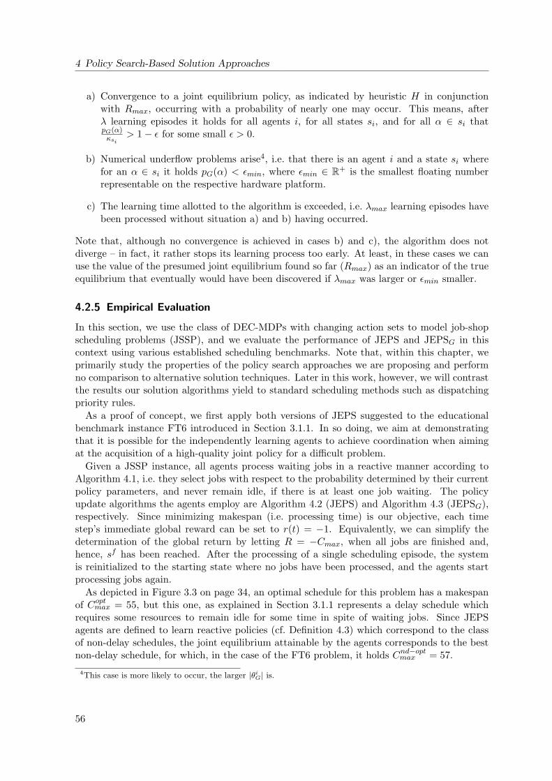
4 Policy Search-Based Solution Approaches
a) Convergence to a joint equilibrium policy, as indicated by heuristic H in conjunctionwith Rmax, occurring with a probability of nearly one may occur. This means, afterλ learning episodes it holds for all agents i, for all states si, and for all α ∈ si thatpG(α)κsi
> 1− ε for some small ε > 0.
b) Numerical underflow problems arise4, i.e. that there is an agent i and a state si wherefor an α ∈ si it holds pG(α) < εmin, where εmin ∈ R+ is the smallest floating numberrepresentable on the respective hardware platform.
c) The learning time allotted to the algorithm is exceeded, i.e. λmax learning episodes havebeen processed without situation a) and b) having occurred.
Note that, although no convergence is achieved in cases b) and c), the algorithm does notdiverge – in fact, it rather stops its learning process too early. At least, in these cases we canuse the value of the presumed joint equilibrium found so far (Rmax) as an indicator of the trueequilibrium that eventually would have been discovered if λmax was larger or εmin smaller.
4.2.5 Empirical Evaluation
In this section, we use the class of DEC-MDPs with changing action sets to model job-shopscheduling problems (JSSP), and we evaluate the performance of JEPS and JEPSG in thiscontext using various established scheduling benchmarks. Note that, within this chapter, weprimarily study the properties of the policy search approaches we are proposing and performno comparison to alternative solution techniques. Later in this work, however, we will contrastthe results our solution algorithms yield to standard scheduling methods such as dispatchingpriority rules.
As a proof of concept, we first apply both versions of JEPS suggested to the educationalbenchmark instance FT6 introduced in Section 3.1.1. In so doing, we aim at demonstratingthat it is possible for the independently learning agents to achieve coordination when aimingat the acquisition of a high-quality joint policy for a difficult problem.
Given a JSSP instance, all agents process waiting jobs in a reactive manner according toAlgorithm 4.1, i.e. they select jobs with respect to the probability determined by their currentpolicy parameters, and never remain idle, if there is at least one job waiting. The policyupdate algorithms the agents employ are Algorithm 4.2 (JEPS) and Algorithm 4.3 (JEPSG),respectively. Since minimizing makespan (i.e. processing time) is our objective, each timestep’s immediate global reward can be set to r(t) = −1. Equivalently, we can simplify thedetermination of the global return by letting R = −Cmax, when all jobs are finished and,hence, sf has been reached. After the processing of a single scheduling episode, the systemis reinitialized to the starting state where no jobs have been processed, and the agents startprocessing jobs again.
As depicted in Figure 3.3 on page 34, an optimal schedule for this problem has a makespanof Coptmax = 55, but this one, as explained in Section 3.1.1 represents a delay schedule whichrequires some resources to remain idle for some time in spite of waiting jobs. Since JEPSagents are defined to learn reactive policies (cf. Definition 4.3) which correspond to the classof non-delay schedules, the joint equilibrium attainable by the agents corresponds to the bestnon-delay schedule, for which, in the case of the FT6 problem, it holds Cnd−optmax = 57.
4This case is more likely to occur, the larger |θiG| is.
56
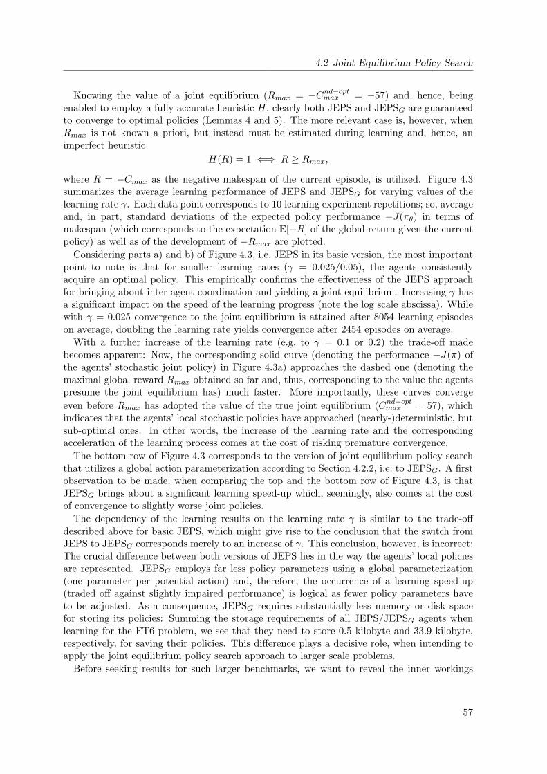
4.2 Joint Equilibrium Policy Search
Knowing the value of a joint equilibrium (Rmax = −Cnd−optmax = −57) and, hence, beingenabled to employ a fully accurate heuristic H, clearly both JEPS and JEPSG are guaranteedto converge to optimal policies (Lemmas 4 and 5). The more relevant case is, however, whenRmax is not known a priori, but instead must be estimated during learning and, hence, animperfect heuristic
H(R) = 1 ⇐⇒ R ≥ Rmax,
where R = −Cmax as the negative makespan of the current episode, is utilized. Figure 4.3summarizes the average learning performance of JEPS and JEPSG for varying values of thelearning rate γ. Each data point corresponds to 10 learning experiment repetitions; so, averageand, in part, standard deviations of the expected policy performance −J(πθ) in terms ofmakespan (which corresponds to the expectation E[−R] of the global return given the currentpolicy) as well as of the development of −Rmax are plotted.
Considering parts a) and b) of Figure 4.3, i.e. JEPS in its basic version, the most importantpoint to note is that for smaller learning rates (γ = 0.025/0.05), the agents consistentlyacquire an optimal policy. This empirically confirms the effectiveness of the JEPS approachfor bringing about inter-agent coordination and yielding a joint equilibrium. Increasing γ hasa significant impact on the speed of the learning progress (note the log scale abscissa). Whilewith γ = 0.025 convergence to the joint equilibrium is attained after 8054 learning episodeson average, doubling the learning rate yields convergence after 2454 episodes on average.
With a further increase of the learning rate (e.g. to γ = 0.1 or 0.2) the trade-off madebecomes apparent: Now, the corresponding solid curve (denoting the performance −J(π) ofthe agents’ stochastic joint policy) in Figure 4.3a) approaches the dashed one (denoting themaximal global reward Rmax obtained so far and, thus, corresponding to the value the agentspresume the joint equilibrium has) much faster. More importantly, these curves convergeeven before Rmax has adopted the value of the true joint equilibrium (Cnd−optmax = 57), whichindicates that the agents’ local stochastic policies have approached (nearly-)deterministic, butsub-optimal ones. In other words, the increase of the learning rate and the correspondingacceleration of the learning process comes at the cost of risking premature convergence.
The bottom row of Figure 4.3 corresponds to the version of joint equilibrium policy searchthat utilizes a global action parameterization according to Section 4.2.2, i.e. to JEPSG. A firstobservation to be made, when comparing the top and the bottom row of Figure 4.3, is thatJEPSG brings about a significant learning speed-up which, seemingly, also comes at the costof convergence to slightly worse joint policies.
The dependency of the learning results on the learning rate γ is similar to the trade-offdescribed above for basic JEPS, which might give rise to the conclusion that the switch fromJEPS to JEPSG corresponds merely to an increase of γ. This conclusion, however, is incorrect:The crucial difference between both versions of JEPS lies in the way the agents’ local policiesare represented. JEPSG employs far less policy parameters using a global parameterization(one parameter per potential action) and, therefore, the occurrence of a learning speed-up(traded off against slightly impaired performance) is logical as fewer policy parameters haveto be adjusted. As a consequence, JEPSG requires substantially less memory or disk spacefor storing its policies: Summing the storage requirements of all JEPS/JEPSG agents whenlearning for the FT6 problem, we see that they need to store 0.5 kilobyte and 33.9 kilobyte,respectively, for saving their policies. This difference plays a decisive role, when intending toapply the joint equilibrium policy search approach to larger scale problems.
Before seeking results for such larger benchmarks, we want to reveal the inner workings
57
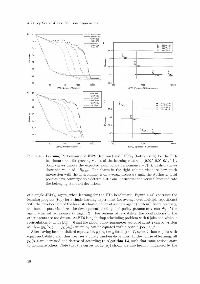
4 Policy Search-Based Solution Approaches
Figure 4.3: Learning Performance of JEPS (top row) and JEPSG (bottom row) for the FT6benchmark and for growing values of the learning rate γ ∈ 0.025, 0.05, 0.1, 0.2.Solid curves denote the expected joint policy performance −J(π), dashed curvesshow the value of −Rmax. The charts in the right column visualize how muchinteraction with the environment is on average necessary until the stochastic localpolicies have converged to a deterministic one; horizontal and vertical lines indicatethe belonging standard deviations.
of a single JEPSG agent, when learning for the FT6 benchmark. Figure 4.4a) contrasts thelearning progress (top) for a single learning experiment (no average over multiple repetitions)with the development of the local stochastic policy of a single agent (bottom). More precisely,the bottom part visualizes the development of the global policy parameter vector θ2
G of theagent attached to resource r2 (agent 2). For reasons of readability, the local policies of theother agents are not drawn. As FT6 is a job-shop scheduling problem with 6 jobs and withoutrecirculation, it holds |Ari | = 6 and the global policy parameter vector of agent 2 can be writtenas θ2
G = (pG(α1), . . . , pG(α6)) where αj can be equated with a certain job j ∈ J .After having been initialized equally, i.e. pG(αj) = 1
6 for all j ∈ J , agent 2 chooses jobs withequal probability and, thus, realizes a purely random dispatcher. In the course of learning, allpG(αj) are increased and decreased according to Algorithm 4.3, such that some actions startto dominate others. Note that the curves for pG(αj) shown are also heavily influenced by the
58
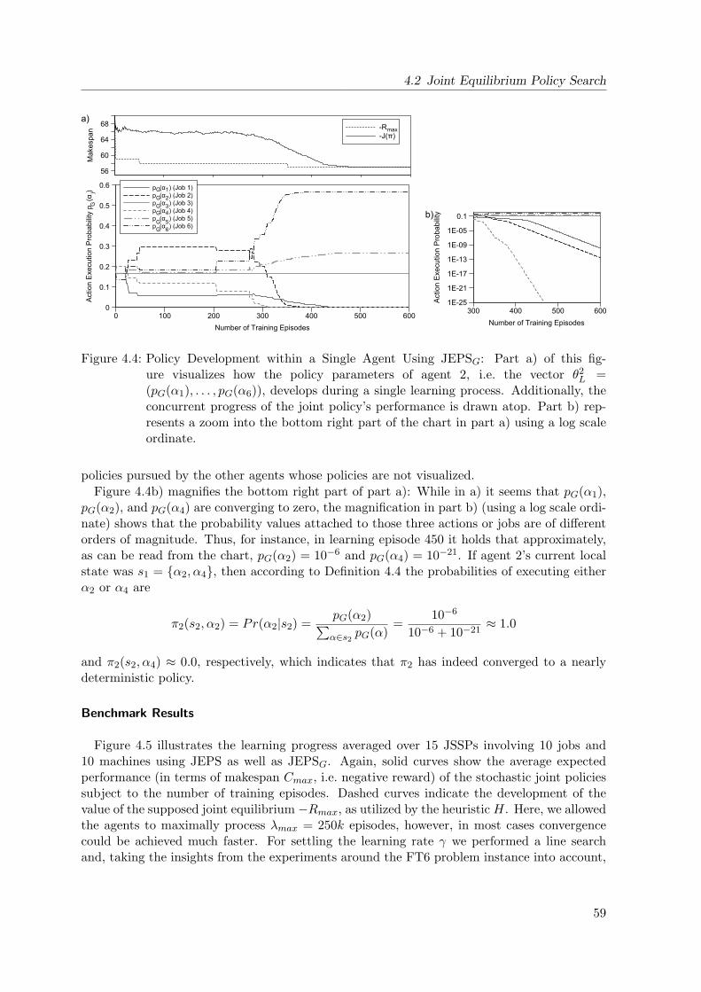
4.2 Joint Equilibrium Policy Search
Figure 4.4: Policy Development within a Single Agent Using JEPSG: Part a) of this fig-ure visualizes how the policy parameters of agent 2, i.e. the vector θ2
L =(pG(α1), . . . , pG(α6)), develops during a single learning process. Additionally, theconcurrent progress of the joint policy’s performance is drawn atop. Part b) rep-resents a zoom into the bottom right part of the chart in part a) using a log scaleordinate.
policies pursued by the other agents whose policies are not visualized.Figure 4.4b) magnifies the bottom right part of part a): While in a) it seems that pG(α1),
pG(α2), and pG(α4) are converging to zero, the magnification in part b) (using a log scale ordi-nate) shows that the probability values attached to those three actions or jobs are of differentorders of magnitude. Thus, for instance, in learning episode 450 it holds that approximately,as can be read from the chart, pG(α2) = 10−6 and pG(α4) = 10−21. If agent 2’s current localstate was s1 = α2, α4, then according to Definition 4.4 the probabilities of executing eitherα2 or α4 are
π2(s2, α2) = Pr(α2|s2) =pG(α2)∑α∈s2 pG(α)
=10−6
10−6 + 10−21≈ 1.0
and π2(s2, α4) ≈ 0.0, respectively, which indicates that π2 has indeed converged to a nearlydeterministic policy.
Benchmark Results
Figure 4.5 illustrates the learning progress averaged over 15 JSSPs involving 10 jobs and10 machines using JEPS as well as JEPSG. Again, solid curves show the average expectedperformance (in terms of makespan Cmax, i.e. negative reward) of the stochastic joint policiessubject to the number of training episodes. Dashed curves indicate the development of thevalue of the supposed joint equilibrium −Rmax, as utilized by the heuristic H. Here, we allowedthe agents to maximally process λmax = 250k episodes, however, in most cases convergencecould be achieved much faster. For settling the learning rate γ we performed a line searchand, taking the insights from the experiments around the FT6 problem instance into account,
59
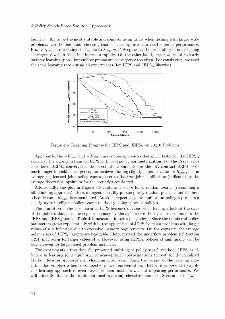
4 Policy Search-Based Solution Approaches
found γ = 0.1 to be the most suitable and compromising value, when dealing with larger-scaleproblems. On the one hand, choosing smaller learning rates can yield superior performance.However, when restricting the agents to λmax = 250k episodes, the probability of not reachingconvergence within that time increases rapidly. On the other hand, larger values of γ clearlyincrease learning speed, but enforce premature convergence too often. For consistency, we usedthe same learning rate during all experiments (for JEPS and JEPSG likewise).
Figure 4.5: Learning Progress for JEPS and JEPSG on 10x10 Problems
Apparently, the −Rmax and −J(πθ) curves approach each other much faster for the JEPSGvariant of the algorithm than for JEPS with local policy parameterization. For the 15 scenariosconsidered, JEPSG converges at the latest after about 11k episodes. By contrast, JEPS needsmuch longer to yield convergence, but achieves finding slightly superior values of Rmax, i.e. onaverage the learned joint policy comes closer to the true joint equilibrium (indicated by theaverage theoretical optimum for the scenarios considered).
Additionally, the plot in Figure 4.5 contains a curve for a random search (resembling ahill-climbing approach): Here, all agents steadily pursue purely random policies, and the bestschedule (best Rmax) is remembered. As to be expected, joint equilibrium policy represents aclearly more intelligent policy search method yielding superior policies.
The limitation of the basic form of JEPS becomes obvious when having a look at the sizesof the policies that must be kept in memory by the agents (see the rightmost columns in theJEPS and JEPSG part of Table 4.1, measured in bytes per policy). Since the number of policyparameters grows exponentially with n, the application of JEPS for m×n problems with largervalues of n is infeasible due to excessive memory requirements. On the contrary, the averagepolicy sizes of JEPSG agents are negligible. Here, instead the underflow problem (cf. Section4.2.4) may occur for larger values of n. However, using JEPSG, policies of high quality can belearned even for larger-sized problem instances.
The experiments stress that the presented multi-agent policy search method, JEPS, is ef-fective in learning joint equilibria, or near-optimal approximations thereof, for decentralizedMarkov decision processes with changing action sets. Using the variant of the learning algo-rithm that employs a highly compacted policy representation, JEPSG, it is possible to applythis learning approach to even larger problem instances without impairing performance. Wewill critically discuss the results obtained in a comprehensive manner in Section 4.4 below.
60
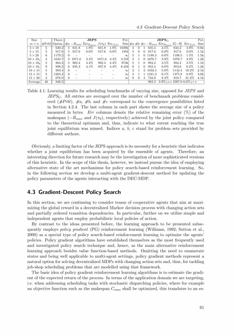
4.3 Gradient-Descent Policy Search
Size Theor. JEPS Pol. JEPSG Pol.m× n #Prbl Optim. #a −Rmax ErrRmax J(πθ) ErrJ(π) Size #a #b #c −Rmax ErrRmax E[−R] ErrJ(π) Size
5× 10 5 620.2 5 631.8 1.9% 631.8 1.9% 1029k 4 0 1 635.4 2.5% 644.2 3.9% 0.6k5× 15 5 917.6 5 917.6 0.0% 917.6 0.0% 18M 5 0 0 917.6 0.0% 917.6 0.0% 1.1k5× 20 6 1179.2 0 - - - - ∞ 5 1 0 1188.3 0.8% 1196.5 1.5% 1.5k
10× 10a 3 1035.7 3 1071.0 3.4% 1071.0 3.4% 3.5M 3 1 0 1076.7 3.9% 1076.7 3.9% 1.2k10× 10b 5 864.2 5 902.4 4.4% 902.4 4.4% 973k 5 1 0 894.2 3.5% 894.2 3.5% 1.1k10× 10c 9 898.2 8 935.3 4.1% 937.9 4.4% 6.4M 8 1 0 952.4 6.0% 953.6 6.2% 1.2k10× 15 5 983.4 0 - - - - ∞ 2 1 2 1032.4 5.0% 1142.4 16.2% 2.1k15× 15 5 1263.2 0 - - - - ∞ 3 1 1 1341.2 6.1% 1375.8 8.9% 3.0k15× 20 3 676.0 0 - - - - ∞ 0 0 3 732.0 8.3% 819.7 21.2% 4.1kAverage 46 946.5 983.3 3.9%±3.3 1007.0 6.6%±7.3
Table 4.1: Learning results for scheduling benchmarks of varying size, opposed for JEPS andJEPSG. All entries are averaged over the number of benchmark problems consid-ered (#Prbl), #a, #b, and #c correspond to the convergence possibilities listedin Section 4.2.4. The last column in each part shows the average size of a policymeasured in bytes. Err columns denote the relative remaining error (%) of themakespan (−Rmax and J(πθ), respectively) achieved by the joint policy comparedto the theoretical optimum and, thus, indicate to what extent reaching the truejoint equilibrium was missed. Indices a, b, c stand for problem sets provided bydifferent authors.
Obviously, a limiting factor of the JEPS approach is its necessity for a heuristic that indicateswhether a joint equilibrium has been acquired by the ensemble of agents. Therefore, aninteresting direction for future research may be the investigation of more sophisticated versionsof this heuristic. In the scope of this thesis, however, we instead pursue the idea of employingalternative state of the art mechanisms for policy search-based reinforcement learning. So,in the following section we develop a multi-agent gradient-descent method for updating thepolicy parameters of the agents interacting with the DEC-MDP.
4.3 Gradient-Descent Policy Search
In this section, we are continuing to consider teams of cooperative agents that aim at maxi-mizing the global reward in a decentralized Markov decision process with changing action setsand partially ordered transition dependencies. In particular, further on we utilize simple andindependent agents that employ probabilistic local policies of action.
By contrast to the ideas presented before, the learning approach to be presented subse-quently employs policy gradient (PG) reinforcement learning (Williams, 1992; Sutton et al.,2000) as a special type of policy search-based reinforcement learning to optimize the agents’policies. Policy gradient algorithms have established themselves as the most frequently usedand investigated policy search technique and, hence, as the main alternative reinforcementlearning approach besides value function-based methods. Omitting the need to enumeratestates and being well applicable to multi-agent settings, policy gradient methods represent anatural option for solving decentralized MDPs with changing action sets and, thus, for tacklingjob-shop scheduling problems that are modelled using that framework.
The basic idea of policy gradient reinforcement learning algorithms is to estimate the gradi-ent of the expected return of the process. In terms of the application domain we are targeting,i.e. when addressing scheduling tasks with stochastic dispatching policies, where for examplean objective function such as the makespan Cmax shall be optimized, this translates to an es-
61
4 Policy Search-Based Solution Approaches
timate of the gradient of the makespan of the resulting schedule, which is derived with respectto a set of real-valued policy parameters. These parameters make up the agents’ stochasticpolicies and determine their dispatching behavior. To this end, we will suggest a compactrepresentation of the agents’ local policies that can also directly be mapped to a completeselection of a disjunctive graph for the problem at hand. Following the gradient by adjustingthe policy parameters’ values (and assuming the correctness of the gradient estimate), it isguaranteed that the expected return of the policy is improved, i.e. that schedules that arebetter in terms of makespan are created with higher probability.
4.3.1 Gradient-Descent Policy Learning
As explained in Section 4.1.1, the general idea of policy optimization in reinforcement learningis to optimize the policy parameter vector θ such that the policy performance J(πθ) definedas the sum of immediate global rewards (Equation 4.1) is maximized. When employing mindependently acting and learning agents, each one strives for optimizing its own parameterset θi optimizing its corresponding local policy πθi .
In this section, we introduce the concept of gradient-descent policy learning for one singleagent, i.e. we assume a single entity controlling action choices and, in so doing, can disregardthe agent-specific indices i (e.g. an experience sequence then is the history of states, actions,and rewards of the action, and no longer a collection of sequences 〈h1, . . . , hm〉). Thereafter(Section 4.3.2), we generalize these ideas to the multi-agent case.
Single-Agent Policy Gradient Estimation
Assuming a single agent interacting with its environment (MDP), this central authority collectsan experience sequence (adapted from Definition 4.2)
h = [s(0), a(0), r(0), s(1), . . . , s(D − 1), a(D − 1), r(D − 1), s(D)]
of length D using its policy πθ which is parameterized by parameter vector θ = (θ1, . . . , θu)(u ≥ 1 denotes the number of parameters used). Policy gradient methods follow the steepestdescent on the expected return. This requires that the policy performance J(πθ) must bedifferentiable with respect to each component θk of the parameter vector θ. It holds
∇θkJ(πθ) = ∇θkE
[D−1∑d=0
γkr(k)|πθ
]= ∇θk
∑h∈H
Pr(h|θ)R(h) (4.4)
where H denotes the space of all possible experience sequences. R(h) corresponds to the returncollected in one specific episode (experience sequence) that is denoted by h and that arose usingcurrent policy parameters θ. Exploiting the properties of the log likelihood, Equation 4.4 canbe written as
∇θkJ(πθ) =∑h∈H
R(h)∇θkPr(h|θ)Pr(h|θ)
Pr(h|θ)
= E [R(h)∇θk lnPr(h|θ)|πθ] . (4.5)
62
4.3 Gradient-Descent Policy Search
The term Pr(h|θ) needs some more profound consideration. It denotes the probability that anexperience sequence h is created given that the agent chooses its actions according to the policydefined through parameters θ. This probability can be defined recursively: Let HD denotethe space of sequences of length D. Given a shortened experience sequence hD−1 ∈ HD−1 andassuming knowledge of Pr(hD−1|θ), the probability of hD can be computed by multiplyingPr(hD−1|θ) with (a) the probability of executing action a(D − 1) depending on hD−1 andpolicy πθ, (b) the probability of receiving reward r(D− 1) given s(D− 1), a(D− 1) and s(D),and (c) the probability of entering s(D) given s(D − 1) and a(D − 1). Thus,
Pr(hD|θ) = Pr(hD−1|θ) · Pr(a(D − 1)|hD−1, πθ)·Pr(r(D − 1)|s(D − 1), a(D − 1), s(D)) · Pr(s(D)|s(D − 1), a(D − 1))
= Pr(hD−1|θ) · πθ(s(D − 1, hD−1), a(D − 1))·r(s(D − 1), a(D − 1), s(D)) · p(s(D − 1), a(D − 1), s(D)),
where functions r and p are the reward and transition function of the underlying MDP, andbased on this recursive formulation, we can state the following auxiliary lemma.
Lemma 6. Given an experience sequence hD of length D and a policy πθ that parameterizesthe single agent’s actions through parameters θ = (θ1, . . . , θu), it holds for all θk (1 ≤ k ≤ u)
∇θk lnPr(hD|θ) =D−1∑d=0
∇θk lnπθ(s(d, hD), a(d, hD)) (4.6)
where s(d, hD) denotes the sequence of the first d+ 1 states from hD (cf. Definition 4.2).
Proof. By induction over D.Induction Base Case: D = 0. The set H0 contains only one single element h = [s(0)] which iswhy Pr(h|θ) = 1 and ∇θk lnPr(h|θ) = 0 for all j. The right-hand side of Equation 4.6 is 0 asit represents an empty sum. Thus, the base case holds.Induction Assumption: For all experience sequences hD ∈ HD of length D Equation 4.6 holds.Induction Hypothesis: For all experience sequences h ∈ HD+1 of length D + 1 it holds
∇θk lnPr(hD+1|θ) =D∑d=0
∇θk lnπθ(s(d, hD+1), a(d, hD+1)).
Induction Step: Let hD+1 = [s(0), a(0), r(0), s(1), . . . , s(D), a(D), r(D), s(D + 1)] ∈ HD+1 bean experience sequence of length D + 1 and hD ∈ HD its prefix of length D. Then, by therecursive definition of Pr(h|θ) we have
∇θk lnPr(hD+1|θ)= ∇θk ln
(Pr(hD|θ)Pr(a(D)|hD, πθ)Pr(r(D)|s(D), a(D), s(D+1))Pr(s(D+1)|s(D), a(D))
)= ∇θk lnPr(hD|θ) +∇θk lnπθ(s(D,hD), a(D))
+∇θk ln r(s(D), a(D), s(D + 1)) +∇θk ln p(s(D), a(D), s(D + 1)).
The third and fourth term of this sum evaluate to zero as the state transition and reward
63
4 Policy Search-Based Solution Approaches
probabilities do not depend on θk. Using the induction assumption, we obtain
∇θk lnPr(hD+1|θ) =D−1∑d=0
∇θk lnπθ(s(d, hD), a(d, hD)) +∇θk lnπθ(s(D,hD), a(D))
=D∑d=0
∇θk lnπθ(s(d, hD+1), a(d, hD+1)).
Lemma 6 allows us to determine the log derivative of Pr(h|θ) with respect to any policyparameter without the need for an explicit representation of that distribution. The onlyrequirement that must be fulfilled is that the policy πθ must be differentiable with respect toany θk. Rewriting Equation 4.5, we can express the gradient of a policy’s performance as
∇θkJ(πθ) = E
[R(h)
Dh−1∑d=0
∇θk lnπθ(s(d, h), a(d, h))
]
=∑h∈H
R(h)Pr(h|θ)
(Dh−1∑d=0
∇θk lnπθ(s(d, h), a(d, h))
), (4.7)
where Dh denotes the length of a specific sequence h.It must be emphasized that an exact computation of the gradient ∇θJ(πθ) becomes quickly
intractable as the problem size grows. Therefore, throughout this chapter, we revert to deter-mining Monte-Carlo estimates of the gradient, similar to related work (Williams, 1992; Suttonet al., 2000; Peshkin et al., 2000), generated from a samples set E of experience sequences.Consequently, when applying Equation 4.7, the outer sum does not run over h ∈ H, but overh ∈ E instead.
Updating the Policy
An update to the agents’ policy parameters θ = (θ1, . . . , θu) uses for all k ∈ 1, . . . , u thestandard rule
θk ← θk + βb∇θkJ(πθ) (4.8)
where βb ∈ R+ denotes a learning rate.If b ∈ N counts the number of policy updates made and
∑b βb =∞,
∑b β
2b = const, then the
learning process is guaranteed to converge to a local optimum, at least. The policy gradientupdate scheme realized resembles the episodic Reinforce gradient estimator (Williams, 1992).For various applications, the fact that this algorithm estimates the gradient for a dedicatedrecurrent state, is problematic. Hence, other algorithms, such as GPOMDP (Baxter andBartlett, 1999) or the natural actor critic (NAC, Peters et al., 2005), were suggested that areintended to overcome the need of identifying a specific recurrent state. Meanwhile, they comeat the cost of introducing a bias to the gradient estimate and trading this off against reducingvariance. Because, for DEC-MDPs with changing action sets and partially ordered transitiondependencies which will return into the center of our interest subsequently, a recurrent state(starting state) is naturally available, we keep with doing the gradient calculation using thelikelihood ratio method described.
64
4.3 Gradient-Descent Policy Search
4.3.2 Independent Agents and Decentralized Policy Gradient
The line of arguments given in the previous section assumed a single agent executing solitaryactions. We now return to the consideration of m-agent factored DEC-MDP environmentswhere the actions can be broken up into m partial, or local actions.
As specified in Definition 2.9, the joint policy π is defined as the tuple of m local policies,i.e. π = 〈π1, . . . , πm〉. We assume that the policy πi of each agent i is defined through a smallset of parameters θi = (θi1, . . . , θ
iui) where all θik ∈ R. These parameter vectors form the basis
for defining probabilistic agent-specific policies of action.Accordingly, the parameter vector for the joint policy is made up of the concatenation of all
local policies’ parameters: θ = (θ1, . . . , θm). For clarity of notation, in the remainder of thischapter we will denote local policies by πθi (instead of πi) to stress their dependency on theirparameters θi.
Our goal retains to perform gradient descent-based policy search under these conditionswhere, in analogy to the single agent case, we also estimate the gradient of policy performanceusing Monte-Carlo methods. In what follows, we distinguish between two different approachesto action execution and gradient-descent policy search-based learning.
a) Joint Control and Learning This corresponds to a central authority that takes actions andperforms learning updates. Insofar, it resembles the single agent case from Section 4.3.1to some extent. However, since we are addressing m-agent factored DEC-MDPs we as-sume that any action must be split into m independent components. Therefore, thisapproach explicitly considers joint policies πθ = 〈πθ1 , . . . , πθm〉 and executes joint ac-tions a = (a1, . . . , am), though each partial policy πθi is represented by its own set ofparameters θi.
Under these assumptions the gradient of policy performance can be expressed5 as
∇θJ(πθ) =∑h∈H
R(h)Pr(h|θ)
(Dh−1∑d=0
∇θ lnπθ(s(d, h), a(d, h))
)(4.9)
where πθ is composed as the product of πθi (for i = 1, . . . ,m)
πθ(s, a) =m∏i=1
πθi(si, ai) (4.10)
and where a = (a1, . . . , am) and h = 〈h1, . . . , hm〉 denote joint actions and joint experi-ence sequences, respectively (cf. Definitions 2.5 and 4.2).
b) Decentralized Control and Learning While we have mentioned the former approach forreference, the fully decentralized approach is the one that we consistently pursue in thisthesis: We have m independent agents that select their actions independently using theirlocal policies πθi that are specified through parameters θi = (θi1, . . . , θ
iui). Furthermore,
we equip each agent with the same policy gradient algorithm to update its local policy.
Under these assumptions the gradient of policy performance can be expressed as
∇θiJ(πθ) =∑hi∈Hi
R(hi)Pr(hi|θ)
Dhi−1∑d=0
∇θi lnπθi(si(d, hi), a(d, hi))
(4.11)
5 Recall that s(d, h) and a(d, h) access the dth state and action of sequence h.
65
4 Policy Search-Based Solution Approaches
with the distinctive feature that each agent i calculates its individual gradient ∇θiJ(πθ)based on local information stored in agent-specific experience sequences hi.
Needless to say, that the factorization of action choice and execution we assume results inthe fact that any of the two approaches outlined can represent only a subset of policies thata central non-factored controller (corresponding to, for example, the single agent case) canimplement. Therefore, when subsequently speaking about learning updates made to policieswe have to keep in mind that a factored learning approach can at best yield the best set oflocal policies from the restricted class of factored policies.
One may wonder how decentralized policy gradient learning (approach b)) relates to updatesthat are performed by a central learning authority (approach a)). As it turns out, bothapproaches produce identical results: As shown by Peshkin et al. (2000), gradient-descentpolicy search performed by independent agents (distributed gradient-descent) is identical tojoint gradient descent, i.e. to learning updates made by a central authority, as long as factoredpolicies πθ = 〈πθ1 , . . . , πθm〉 are considered. We adapt their finding to our problem settingsand prove the following theorem.
Theorem 3. Given a factored DEC-MDP controlled by m local policies πθ1 , . . . , πθm thatare parameterized by parameter vectors θ1, . . . , θm, we denote the joint policy realized by π =〈πθ1 , . . . , πθm〉 and by θ = (θ1, . . . , θm) the concatenation of those parameters. Then, thegradient of policy performance GC = ∇θJ(πθ) (Equation 4.9) is equal to the vector of gradientsGD = (∇θ1J(πθ), . . . ,∇θmJ(πθ)) where each ∇θiJ(πθ) (for 1 ≤ i ≤ m, Equation 4.11) isdetermined by an independent agent i.
Proof. For the case of centralized control and learning we can writeθ = (θ1
1, . . . , θ1u1, . . . . . . , θm1 , . . . , θ
mum) .
Accordingly, for each component ∇θik of GC (1 ≤ i ≤ m, 1 ≤ k ≤ ui) there exists a corre-sponding entry within the ith component of GD, i.e. within ∇θi . Let i ∈ 1, . . . ,m andk ∈ 1, . . . , ui. Substituting Equation 4.10 into Equation 4.9 yields
∇θikJ(πθ) =∑h∈H
R(h)Pr(h|θ)
Dh−1∑d=0
∇θik lnm∏j=1
πθj (sj(d, h), aj(d, h))
=
∑h∈H
R(h)Pr(h|θ)
Dh−1∑d=0
m∑j=1
∇θik lnπθj (sj(d, h), aj(d, h))
.
Because, however, the action choice probabilities of one agent do not depend on the policyparameters of any other agent, it holds
∇θik lnπθj (sj(d, h), aj(d, h)) = 0
for all i 6= j and for all k, and the previous expression simplifies to
∇θikJ(πθ) =∑h∈H
R(h)Pr(h|θ)
(Dh−1∑d=0
∇θik lnπθi(si(d, h), ai(d, h))
),
and, since si(d, h) = si(d, hi) and ai(d, h) = ai(d, hi),
∇θikJ(πθ) =∑h∈H
R(h)Pr(h|θ)
(Dh−1∑d=0
∇θik lnπθi(si(d, hi), ai(d, hi))
).
66
4.3 Gradient-Descent Policy Search
Because we consider cooperative agents that receive the same global immediate rewards, thereturn of an episode R(h) equals the return of agent-specific experience sequences R(hi).Finally, we note that∑
h∈H Pr(h|θ)f(hi) =∑〈h1...hm〉∈H Pr(〈h1 . . . hm〉|θ)f(hi) =
∑hi∈Hi Pr(hi|θ)f(hi)
for each function f . Thus, we obtain
∇θikJ(πθ) =∑hi∈Hi
R(hi)Pr(hi|θ)
Dhi−1∑d=0
∇θik lnπθi(si(d, hi), ai(d, hi))
which is equal to the definition of the gradient GD determined in a decentralized manner(Equation 4.11). Hence, both gradients are identical.
Theorem 3 tells that the decentralization of action execution among independent agents hasno effect on the policy gradient estimates. Independent agents that are not aware of theirteammates’ actions and only receive local state information determine the same gradient as acentralized learning algorithm would do. An important requirement to be fulfilled, however, isthat all agents perform simultaneous learning, i.e. update their policies at the same time. Inthe next section, we present an algorithmic realization of the decentralized gradient-descentpolicy search method derived using independent agents that synchronize their learning bymeans of episode endings.
4.3.3 Policy Gradient under Changing Action Sets
In this section, we tailor the policy search-based reinforcement learning approach using gradient-descent outlined above for DEC-MDPs with changing action sets. We repeat that, for thisclass of decentralized decision problems the agents’ local states are fully described by the setof available actions and, hence, the local state spaces Si correspond to the power set over alllocal actions P(Ari ).
Compact Policy Representation
We assume that the policy of each agent i is compactly represented by a small set of parametersθi = (θi1, . . . , θ
in) where all θij ∈ R. In particular, we presume that there is exactly one
parameter for each action from Ari (e.g. for each job the agent can execute when focussingon job-shop scheduling problems). As a shortcut, we refer to the parameter belonging toα ∈ Ari by θiα. Accordingly, for a m × n job-shop scheduling problem (with no recirculationand m operations in each job), we have m agents with n policy parameters, thus a total of mnparameters to fully describe the agents’ joint policy.
The parameter vectors mentioned form the basis for defining probabilistic agent-specificpolicies of action.
Definition 4.5 (Gibbs Policy).Let si ⊆ Ari be the current state of agent i where, as explained before, si is the set containingall actions currently available for agent i. The probability of action Pr(α|si, θi) = πθi(si, α)for policy πθi is for all actions α ∈ Ari defined according to the Gibbs distribution,
πθi(si, α) =
e−θ
iαP
x∈sie−θ
ix
if α ∈ si
0 else
67
4 Policy Search-Based Solution Approaches
so that actions that are currently not available have zero probability of being executed. Again,the joint policy π is the concatenation of local policies 〈πθi , . . . , πθi〉.
With respect to scheduling, the probabilistic action selection scheme according to Definition4.5 represents a stochastic and reactive scheduling policy that, when applied, yields the creationof non-delay schedules. Every time si 6= ∅, an action α ∈ Ari is being executed, i.e. a resourcenever remains idle when jobs are waiting for further processing. As a consequence, all stochasticpolicies (for any values of θi) reach the terminal state sf = (s1, . . . , sm) where all jobs havebeen finished and, hence, for all i it holds that si = ∅. Note that in a later chapter (Chapter6), we relax the restriction of acting purely reactively in order to be able to create schedulesfrom beyond the class of non-delay schedules, too.
As pointed out in Section 4.3.1, a crucial precondition for applying a gradient-descent ap-proach to policy optimization is that an agent’s policy πθi must be differentiable with respectto any component of the parameter vector θi. For the compact policy representation using|Ari | parameters as proposed in Definition 4.5 (Gibbs policy) this naturally holds true. For allθiα (1 ≤ i ≤ m, α ∈ Ari ), si ⊂ Ari , and ai ∈ Ari it holds
∇θiα lnπθi(si, ai) =
1− πθi(si, ai) if ai = α
−πθi(si, ai) else.(4.12)
Consequently, given a set E of experience sequences for agent i, the gradient ∇θiJ(πθ) of thepolicy’s performance can be calculated for each parameter θiα from θi = (θi1, . . . , θ
i|Ari |
) as
∇θiαJ(πθ) =1|E|
∑hi∈E
R(hi)Dhi−1∑d=0
∇θiα lnπθiα(si(d, hi), a(d, hi))
.
Note, that πθi is a reactive policy considering not the sequence si(d, hi) of local states, butonly the most recent observation, which is why in this way search can be performed only in thelimited class of reactive local policies. Moreover, the gradient is not calculated analytically, butsampled in a Monte-Carlo manner by interacting with the environment and, hence, determinedfrom a finite set of experience sequences E ⊂ Hi as noted before.
Finally, we employ the average performance
JE(πθ) =1|E|
∑hi∈E
R(hi)
as a simple baseline to reduce the variance of the gradient estimate (Greensmith et al., 2004).Thus, the component for parameter θiα of the policy gradient estimate becomes
gEα := ∇θiαJ(πθ) =1|E|
∑hi∈E
(R(hi)− JE(πθ))Dhi−1∑d=0
∇θiα lnπθi(si(d, hi), ai(d, hi))
(4.13)
where ∇θiα lnπθi(·) is determined according to Equation 4.12.
Gradient-Descent Policy Update Algorithm
The considerations on gradient-descent policy search (GDPS) made so far in this section leadto the formulation of Algorithm 4.4. This algorithm is meant to be plugged in the generic
68
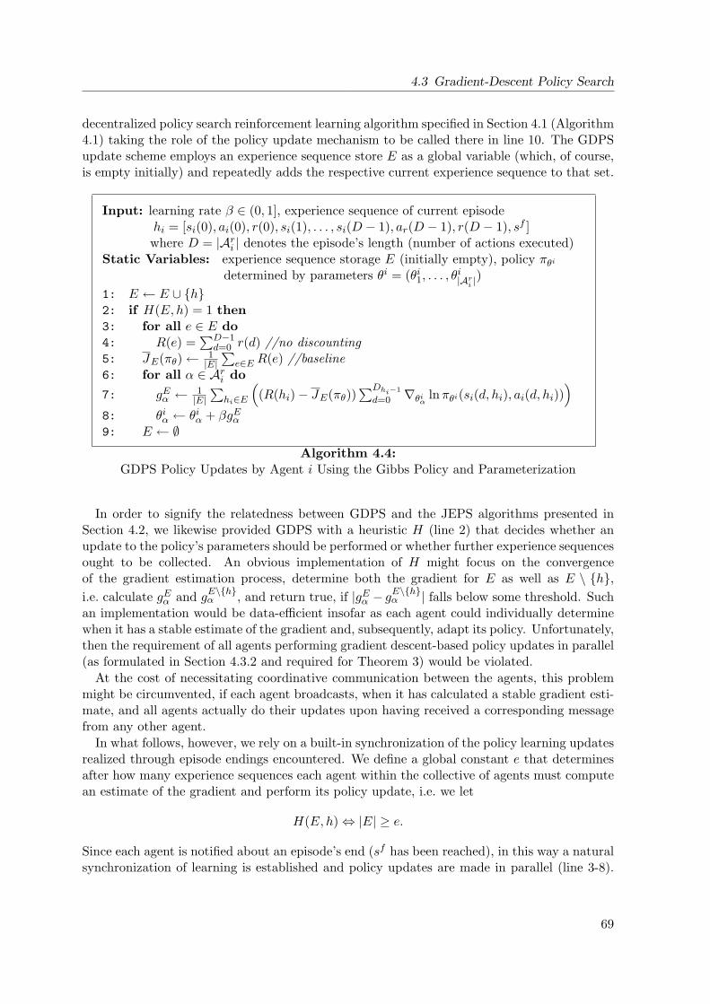
4.3 Gradient-Descent Policy Search
decentralized policy search reinforcement learning algorithm specified in Section 4.1 (Algorithm4.1) taking the role of the policy update mechanism to be called there in line 10. The GDPSupdate scheme employs an experience sequence store E as a global variable (which, of course,is empty initially) and repeatedly adds the respective current experience sequence to that set.
Input: learning rate β ∈ (0, 1], experience sequence of current episodehi = [si(0), ai(0), r(0), si(1), . . . , si(D − 1), ar(D − 1), r(D − 1), sf ]where D = |Ari | denotes the episode’s length (number of actions executed)
Static Variables: experience sequence storage E (initially empty), policy πθidetermined by parameters θi = (θi1, . . . , θ
i|Ari |
)1: E ← E ∪ h2: if H(E, h) = 1 then3: for all e ∈ E do4: R(e) =
∑D−1d=0 r(d) //no discounting
5: JE(πθ)← 1|E|∑
e∈E R(e) //baseline6: for all α ∈ Ari do
7: gEα ← 1|E|∑
hi∈E
((R(hi)− JE(πθ))
∑Dhi−1
d=0 ∇θiα lnπθi(si(d, hi), ai(d, hi)))
8: θiα ← θiα + βgEα9: E ← ∅
Algorithm 4.4:GDPS Policy Updates by Agent i Using the Gibbs Policy and Parameterization
In order to signify the relatedness between GDPS and the JEPS algorithms presented inSection 4.2, we likewise provided GDPS with a heuristic H (line 2) that decides whether anupdate to the policy’s parameters should be performed or whether further experience sequencesought to be collected. An obvious implementation of H might focus on the convergenceof the gradient estimation process, determine both the gradient for E as well as E \ h,i.e. calculate gEα and gE\hα , and return true, if |gEα − g
E\hα | falls below some threshold. Such
an implementation would be data-efficient insofar as each agent could individually determinewhen it has a stable estimate of the gradient and, subsequently, adapt its policy. Unfortunately,then the requirement of all agents performing gradient descent-based policy updates in parallel(as formulated in Section 4.3.2 and required for Theorem 3) would be violated.
At the cost of necessitating coordinative communication between the agents, this problemmight be circumvented, if each agent broadcasts, when it has calculated a stable gradient esti-mate, and all agents actually do their updates upon having received a corresponding messagefrom any other agent.
In what follows, however, we rely on a built-in synchronization of the policy learning updatesrealized through episode endings encountered. We define a global constant e that determinesafter how many experience sequences each agent within the collective of agents must computean estimate of the gradient and perform its policy update, i.e. we let
H(E, h)⇔ |E| ≥ e.
Since each agent is notified about an episode’s end (sf has been reached), in this way a naturalsynchronization of learning is established and policy updates are made in parallel (line 3-8).
69
4 Policy Search-Based Solution Approaches
After that, the experience sequence store E is emptied such that all agent start sampling newexperience sequences using their updated local policies.
4.3.4 Discussion
The GDPS learning algorithm allows for model-free learning in decentralized Markov decisionprocesses where the learning agents have only a partial view of the global system state. Indeveloping the algorithm, we have exploited the properties of DEC-MDPs with changing actionsets and partially ordered transition dependencies – since each action can be executed onlyonce by each learner, a single parameter per action is sufficient for representing local policies.
Gradient-descent algorithms are guaranteed to at least converge to a local optimum in policyspace (Arrow and Hurwicz, 1960). Since a Nash equilibrium also represents a local optimumwhen doing decentralized gradient-descent for a factored controller (Peshkin et al., 2000),it is clear that any Nash equilibrium is a possible point of convergence for GDPS as well.Unfortunately, the reverse is not true: There may be additional local optima in policy space towhich GDPS may converge and which are, in general, of lower value than Nash equilibria. Wehave visualized this situation in Figure 4.6 for a fictional 2-agent example with an extremelyunevenly shaped policy performance function J . Both agents are parameterized by a singleparameter only (θ1 and θ2), drawn along the x- and y-axis in Figure 4.6.
Because a Nash equilibrium denotes a joint policy where no agent can increase the policy’sperformance by changing its local policy single-handedly, we might say that – from a singleagent’s perspective6 – a Nash equilibrium depicts a global optimum. For the toy problem athand, these points of convergence are shown as triangles. Additionally, there are further localoptima in policy space to which a policy gradient method might converge (depending on thestarting point of the search process and the update step size), denoted by circles. Consider,for example, the local optimum marked with a ‘?’ at (θ1, θ2) = (180, 75). Here, apparently,it holds ∇θ1J(πθ) = ∇θ2J(πθ) = 0, which is why GDPS might be attracted by this point.However, (θ1, θ2) does not represent a Nash equilibrium, because a unilateral change of θ1
from 180 to a value larger than 470 by agent 1 would increase J(πθ).Note that Figure 4.6 also highlights the well-known fact that several Nash equilibria of
different value may exist. The one with the highest value (the joint equilibrium, or coordinationequilibrium, cf. Section 4.27) is visualized with a black triangle. On the whole, even if GDPSdoes not provide guarantees for yielding the optimal joint policy, we will show that near-optimaljoint policies of high value can be acquired within little learning time.
Speaking about learning time, the rate of convergence is, of course, strongly influenced bythe learning rate β as well as by the heuristic H that determines after how much interactionwith the environment learning updates to the policies are made by the agents. Concerningthe former we note that, during our empirical experiments (next section), we always useda constant learning rate. Although policy gradient theory actually requires a diminishinglearning rate (as described in Section 4.3.1), we found that not decreasing β during ongoinglearning brings about excellent and convergent results and allows us to omit the introductionof additional parameters controlling the concrete rate of decay of the learning rate.
As denoted above, we employ an implementation of H that initiates policy updates afterhaving sampled a fixed number e of experience sequences by interacting with the DEC-MDP.Clearly, too large a value of e slows down learning in that sampling additional sequences does
6More precisely, from any single agent’s perspective simultaneously.7The case of two joint equilibria with identical value is considered in depth in Section 4.2.3 (cf. Lemma 5).
70
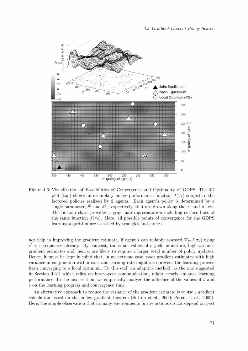
4.3 Gradient-Descent Policy Search
Joint Equilibrium
Nash Equilibrium
Local Optimum (PG)
(policy of agent 1)
(pol
icy
of a
gent
2)
*
−40
−20
0
20
40
60
0
50
100
150
200
250
300
350
100 150 200 250 300 400 450 500
50 100
150 200
250 300
350 400
−10 0
10 20 30 40 50 60
500 400
300 200 100
350
θ1
θ1
θ2
θ2
J(πθ)
Figure 4.6: Visualization of Possibilities of Convergence and Optimality of GDPS: The 3Dplot (top) shows an exemplary policy performance function J(πθ) subject to thefactored policies realized by 2 agents. Each agent’s policy is determined by asingle parameter, θ1 and θ2, respectively, that are drawn along the x- and y-axis.The bottom chart provides a gray map representation including surface lines ofthe same function J(πθ). Here, all possible points of convergence for the GDPSlearning algorithm are sketched by triangles and circles.
not help in improving the gradient estimate, if agent i can reliably assessed ∇θiJ(πθ) usinge′ < e sequences already. By contrast, too small values of e yield immature, high-variancegradient estimates and, hence, are likely to require a larger total number of policy updates.Hence, it must be kept in mind that, in an extreme case, poor gradient estimates with highvariance in conjunction with a constant learning rate might also prevent the learning processfrom converging to a local optimum. To this end, an adaptive method, as the one suggestedin Section 4.3.1 which relies on inter-agent communication, might clearly enhance learningperformance. In the next section, we empirically analyze the influence of the values of β ande on the learning progress and convergence time.
An alternative approach to reduce the variance of the gradient estimate is to use a gradientcalculation based on the policy gradient theorem (Sutton et al., 2000; Peters et al., 2005).Here, the simple observation that in many environments future actions do not depend on past
71
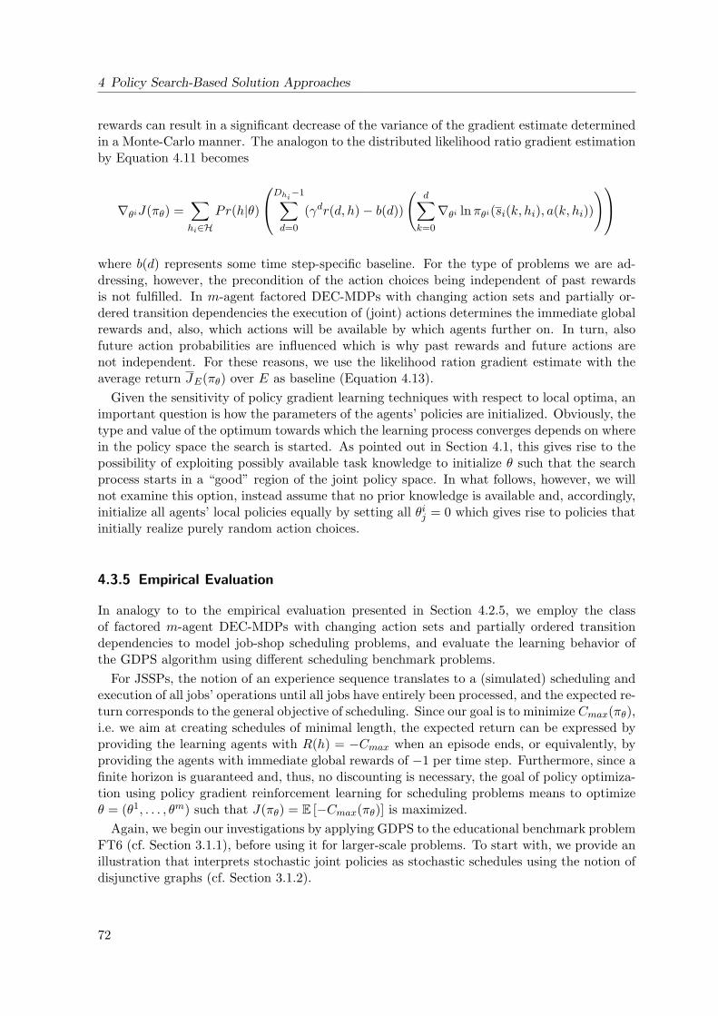
4 Policy Search-Based Solution Approaches
rewards can result in a significant decrease of the variance of the gradient estimate determinedin a Monte-Carlo manner. The analogon to the distributed likelihood ratio gradient estimationby Equation 4.11 becomes
∇θiJ(πθ) =∑hi∈H
Pr(h|θ)
Dhi−1∑d=0
(γdr(d, h)− b(d))
(d∑
k=0
∇θi lnπθi(si(k, hi), a(k, hi))
)where b(d) represents some time step-specific baseline. For the type of problems we are ad-dressing, however, the precondition of the action choices being independent of past rewardsis not fulfilled. In m-agent factored DEC-MDPs with changing action sets and partially or-dered transition dependencies the execution of (joint) actions determines the immediate globalrewards and, also, which actions will be available by which agents further on. In turn, alsofuture action probabilities are influenced which is why past rewards and future actions arenot independent. For these reasons, we use the likelihood ration gradient estimate with theaverage return JE(πθ) over E as baseline (Equation 4.13).
Given the sensitivity of policy gradient learning techniques with respect to local optima, animportant question is how the parameters of the agents’ policies are initialized. Obviously, thetype and value of the optimum towards which the learning process converges depends on wherein the policy space the search is started. As pointed out in Section 4.1, this gives rise to thepossibility of exploiting possibly available task knowledge to initialize θ such that the searchprocess starts in a “good” region of the joint policy space. In what follows, however, we willnot examine this option, instead assume that no prior knowledge is available and, accordingly,initialize all agents’ local policies equally by setting all θij = 0 which gives rise to policies thatinitially realize purely random action choices.
4.3.5 Empirical Evaluation
In analogy to to the empirical evaluation presented in Section 4.2.5, we employ the classof factored m-agent DEC-MDPs with changing action sets and partially ordered transitiondependencies to model job-shop scheduling problems, and evaluate the learning behavior ofthe GDPS algorithm using different scheduling benchmark problems.
For JSSPs, the notion of an experience sequence translates to a (simulated) scheduling andexecution of all jobs’ operations until all jobs have entirely been processed, and the expected re-turn corresponds to the general objective of scheduling. Since our goal is to minimize Cmax(πθ),i.e. we aim at creating schedules of minimal length, the expected return can be expressed byproviding the learning agents with R(h) = −Cmax when an episode ends, or equivalently, byproviding the agents with immediate global rewards of −1 per time step. Furthermore, since afinite horizon is guaranteed and, thus, no discounting is necessary, the goal of policy optimiza-tion using policy gradient reinforcement learning for scheduling problems means to optimizeθ = (θ1, . . . , θm) such that J(πθ) = E [−Cmax(πθ)] is maximized.
Again, we begin our investigations by applying GDPS to the educational benchmark problemFT6 (cf. Section 3.1.1), before using it for larger-scale problems. To start with, we provide anillustration that interprets stochastic joint policies as stochastic schedules using the notion ofdisjunctive graphs (cf. Section 3.1.2).
72
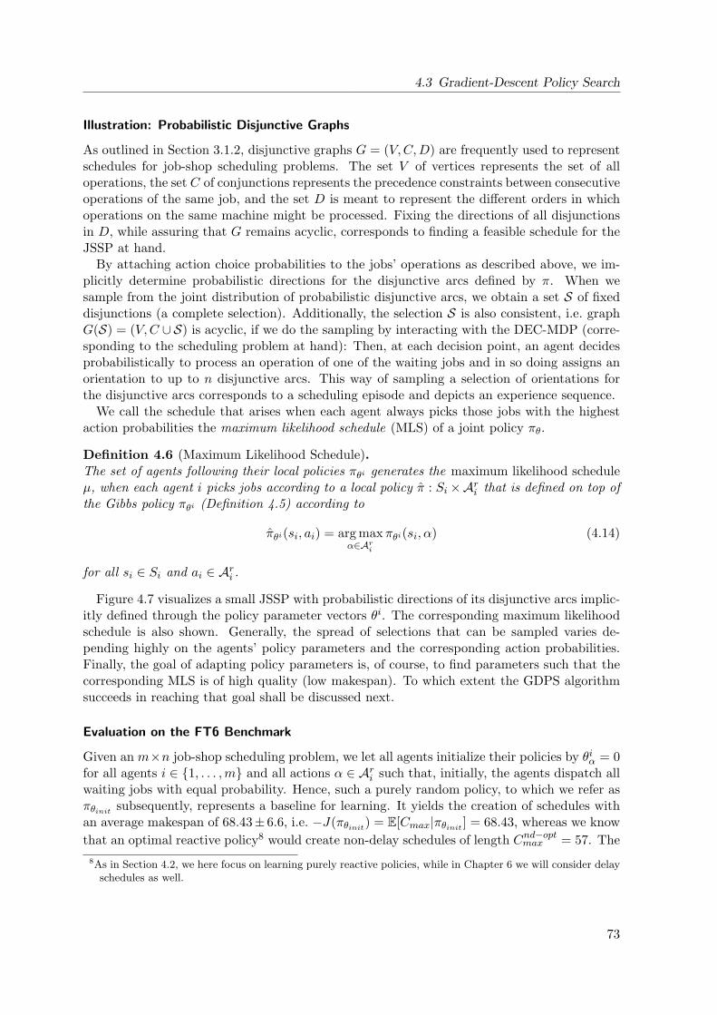
4.3 Gradient-Descent Policy Search
Illustration: Probabilistic Disjunctive Graphs
As outlined in Section 3.1.2, disjunctive graphs G = (V,C,D) are frequently used to representschedules for job-shop scheduling problems. The set V of vertices represents the set of alloperations, the set C of conjunctions represents the precedence constraints between consecutiveoperations of the same job, and the set D is meant to represent the different orders in whichoperations on the same machine might be processed. Fixing the directions of all disjunctionsin D, while assuring that G remains acyclic, corresponds to finding a feasible schedule for theJSSP at hand.
By attaching action choice probabilities to the jobs’ operations as described above, we im-plicitly determine probabilistic directions for the disjunctive arcs defined by π. When wesample from the joint distribution of probabilistic disjunctive arcs, we obtain a set S of fixeddisjunctions (a complete selection). Additionally, the selection S is also consistent, i.e. graphG(S) = (V,C ∪S) is acyclic, if we do the sampling by interacting with the DEC-MDP (corre-sponding to the scheduling problem at hand): Then, at each decision point, an agent decidesprobabilistically to process an operation of one of the waiting jobs and in so doing assigns anorientation to up to n disjunctive arcs. This way of sampling a selection of orientations forthe disjunctive arcs corresponds to a scheduling episode and depicts an experience sequence.
We call the schedule that arises when each agent always picks those jobs with the highestaction probabilities the maximum likelihood schedule (MLS) of a joint policy πθ.
Definition 4.6 (Maximum Likelihood Schedule).The set of agents following their local policies πθi generates the maximum likelihood scheduleµ, when each agent i picks jobs according to a local policy π : Si ×Ari that is defined on top ofthe Gibbs policy πθi (Definition 4.5) according to
πθi(si, ai) = arg maxα∈Ari
πθi(si, α) (4.14)
for all si ∈ Si and ai ∈ Ari .
Figure 4.7 visualizes a small JSSP with probabilistic directions of its disjunctive arcs implic-itly defined through the policy parameter vectors θi. The corresponding maximum likelihoodschedule is also shown. Generally, the spread of selections that can be sampled varies de-pending highly on the agents’ policy parameters and the corresponding action probabilities.Finally, the goal of adapting policy parameters is, of course, to find parameters such that thecorresponding MLS is of high quality (low makespan). To which extent the GDPS algorithmsucceeds in reaching that goal shall be discussed next.
Evaluation on the FT6 Benchmark
Given an m×n job-shop scheduling problem, we let all agents initialize their policies by θiα = 0for all agents i ∈ 1, . . . ,m and all actions α ∈ Ari such that, initially, the agents dispatch allwaiting jobs with equal probability. Hence, such a purely random policy, to which we refer asπθinit subsequently, represents a baseline for learning. It yields the creation of schedules withan average makespan of 68.43± 6.6, i.e. −J(πθinit) = E[Cmax|πθinit ] = 68.43, whereas we knowthat an optimal reactive policy8 would create non-delay schedules of length Cnd−optmax = 57. The
8As in Section 4.2, we here focus on learning purely reactive policies, while in Chapter 6 we will consider delayschedules as well.
73
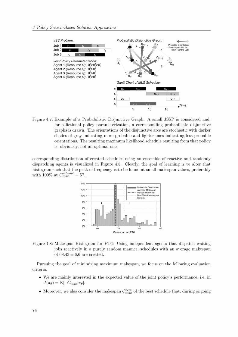
4 Policy Search-Based Solution Approaches
Figure 4.7: Example of a Probabilistic Disjunctive Graph: A small JSSP is considered and,for a fictional policy parameterization, a corresponding probabilistic disjunctivegraphs is drawn. The orientations of the disjunctive arcs are stochastic with darkershades of gray indicating more probable and lighter ones indicating less probableorientations. The resulting maximum likelihood schedule resulting from that policyis, obviously, not an optimal one.
corresponding distribution of created schedules using an ensemble of reactive and randomlydispatching agents is visualized in Figure 4.8. Clearly, the goal of learning is to alter thathistogram such that the peak of frequency is to be found at small makespan values, preferablywith 100% at Cnd−optmax = 57.
Figure 4.8: Makespan Histogram for FT6: Using independent agents that dispatch waitingjobs reactively in a purely random manner, schedules with an average makespanof 68.43± 6.6 are created.
Pursuing the goal of minimizing maximum makespan, we focus on the following evaluationcriteria.
• We are mainly interested in the expected value of the joint policy’s performance, i.e. inJ(πθ) = E[−Cmax|πθ].
• Moreover, we also consider the makespan Cbestmax of the best schedule that, during ongoing
74
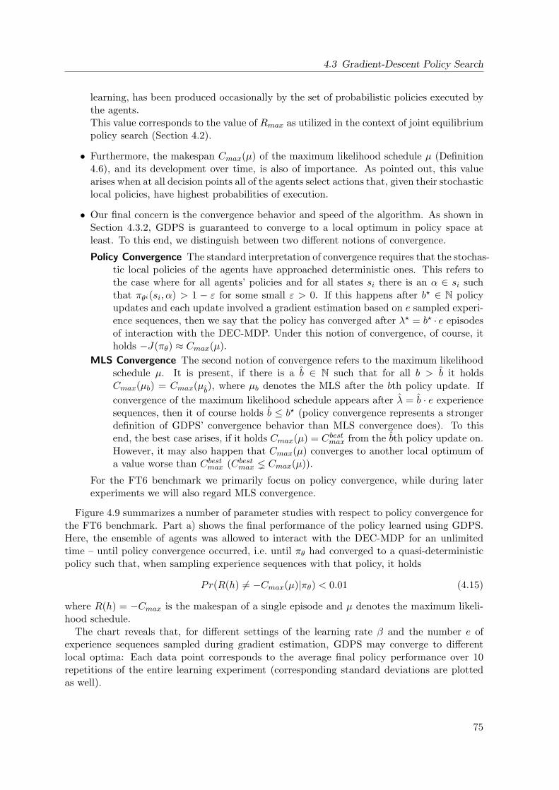
4.3 Gradient-Descent Policy Search
learning, has been produced occasionally by the set of probabilistic policies executed bythe agents.This value corresponds to the value of Rmax as utilized in the context of joint equilibriumpolicy search (Section 4.2).
• Furthermore, the makespan Cmax(µ) of the maximum likelihood schedule µ (Definition4.6), and its development over time, is also of importance. As pointed out, this valuearises when at all decision points all of the agents select actions that, given their stochasticlocal policies, have highest probabilities of execution.
• Our final concern is the convergence behavior and speed of the algorithm. As shown inSection 4.3.2, GDPS is guaranteed to converge to a local optimum in policy space atleast. To this end, we distinguish between two different notions of convergence.
Policy Convergence The standard interpretation of convergence requires that the stochas-tic local policies of the agents have approached deterministic ones. This refers tothe case where for all agents’ policies and for all states si there is an α ∈ si suchthat πθi(si, α) > 1 − ε for some small ε > 0. If this happens after b? ∈ N policyupdates and each update involved a gradient estimation based on e sampled experi-ence sequences, then we say that the policy has converged after λ? = b? · e episodesof interaction with the DEC-MDP. Under this notion of convergence, of course, itholds −J(πθ) ≈ Cmax(µ).
MLS Convergence The second notion of convergence refers to the maximum likelihoodschedule µ. It is present, if there is a b ∈ N such that for all b > b it holdsCmax(µb) = Cmax(µb), where µb denotes the MLS after the bth policy update. Ifconvergence of the maximum likelihood schedule appears after λ = b · e experiencesequences, then it of course holds b ≤ b? (policy convergence represents a strongerdefinition of GDPS’ convergence behavior than MLS convergence does). To thisend, the best case arises, if it holds Cmax(µ) = Cbestmax from the bth policy update on.However, it may also happen that Cmax(µ) converges to another local optimum ofa value worse than Cbestmax (Cbestmax Cmax(µ)).
For the FT6 benchmark we primarily focus on policy convergence, while during laterexperiments we will also regard MLS convergence.
Figure 4.9 summarizes a number of parameter studies with respect to policy convergence forthe FT6 benchmark. Part a) shows the final performance of the policy learned using GDPS.Here, the ensemble of agents was allowed to interact with the DEC-MDP for an unlimitedtime – until policy convergence occurred, i.e. until πθ had converged to a quasi-deterministicpolicy such that, when sampling experience sequences with that policy, it holds
Pr(R(h) 6= −Cmax(µ)|πθ) < 0.01 (4.15)
where R(h) = −Cmax is the makespan of a single episode and µ denotes the maximum likeli-hood schedule.
The chart reveals that, for different settings of the learning rate β and the number e ofexperience sequences sampled during gradient estimation, GDPS may converge to differentlocal optima: Each data point corresponds to the average final policy performance over 10repetitions of the entire learning experiment (corresponding standard deviations are plottedas well).
75
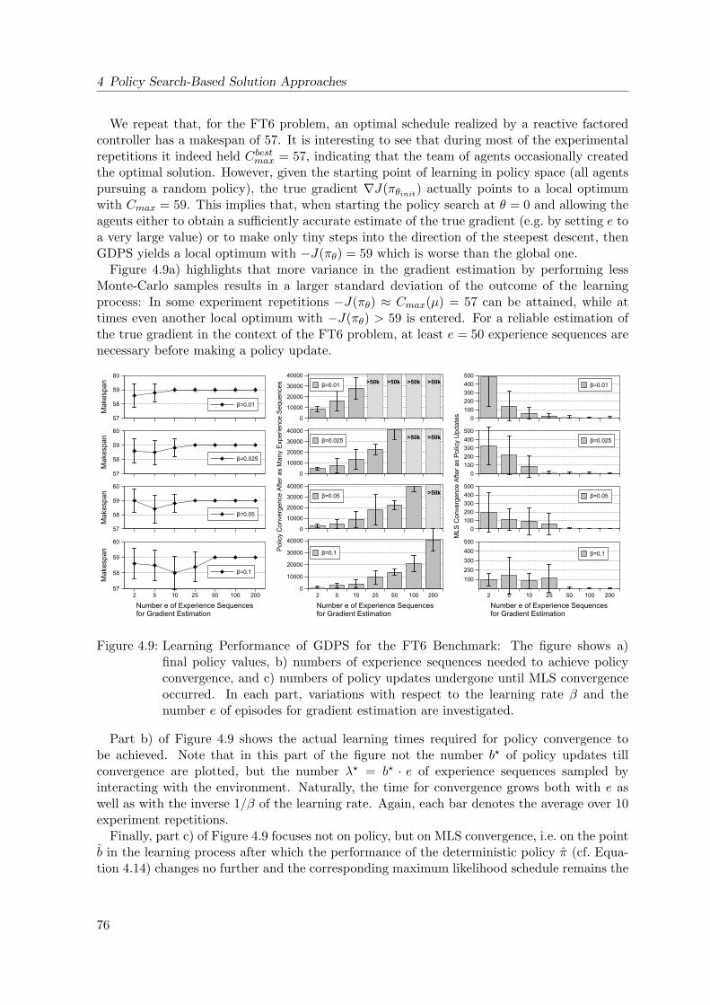
4 Policy Search-Based Solution Approaches
We repeat that, for the FT6 problem, an optimal schedule realized by a reactive factoredcontroller has a makespan of 57. It is interesting to see that during most of the experimentalrepetitions it indeed held Cbestmax = 57, indicating that the team of agents occasionally createdthe optimal solution. However, given the starting point of learning in policy space (all agentspursuing a random policy), the true gradient ∇J(πθinit) actually points to a local optimumwith Cmax = 59. This implies that, when starting the policy search at θ = 0 and allowing theagents either to obtain a sufficiently accurate estimate of the true gradient (e.g. by setting e toa very large value) or to make only tiny steps into the direction of the steepest descent, thenGDPS yields a local optimum with −J(πθ) = 59 which is worse than the global one.
Figure 4.9a) highlights that more variance in the gradient estimation by performing lessMonte-Carlo samples results in a larger standard deviation of the outcome of the learningprocess: In some experiment repetitions −J(πθ) ≈ Cmax(µ) = 57 can be attained, while attimes even another local optimum with −J(πθ) > 59 is entered. For a reliable estimation ofthe true gradient in the context of the FT6 problem, at least e = 50 experience sequences arenecessary before making a policy update.
Figure 4.9: Learning Performance of GDPS for the FT6 Benchmark: The figure shows a)final policy values, b) numbers of experience sequences needed to achieve policyconvergence, and c) numbers of policy updates undergone until MLS convergenceoccurred. In each part, variations with respect to the learning rate β and thenumber e of episodes for gradient estimation are investigated.
Part b) of Figure 4.9 shows the actual learning times required for policy convergence tobe achieved. Note that in this part of the figure not the number b? of policy updates tillconvergence are plotted, but the number λ? = b? · e of experience sequences sampled byinteracting with the environment. Naturally, the time for convergence grows both with e aswell as with the inverse 1/β of the learning rate. Again, each bar denotes the average over 10experiment repetitions.
Finally, part c) of Figure 4.9 focuses not on policy, but on MLS convergence, i.e. on the pointb in the learning process after which the performance of the deterministic policy π (cf. Equa-tion 4.14) changes no further and the corresponding maximum likelihood schedule remains the
76
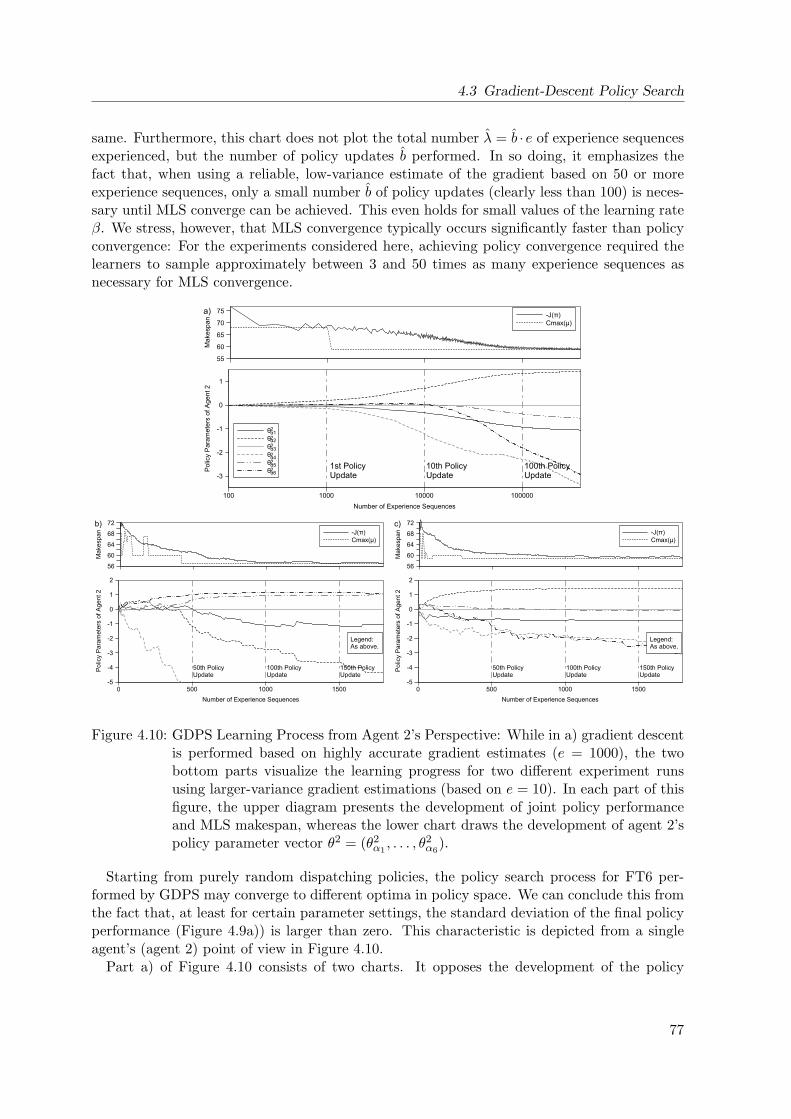
4.3 Gradient-Descent Policy Search
same. Furthermore, this chart does not plot the total number λ = b · e of experience sequencesexperienced, but the number of policy updates b performed. In so doing, it emphasizes thefact that, when using a reliable, low-variance estimate of the gradient based on 50 or moreexperience sequences, only a small number b of policy updates (clearly less than 100) is neces-sary until MLS converge can be achieved. This even holds for small values of the learning rateβ. We stress, however, that MLS convergence typically occurs significantly faster than policyconvergence: For the experiments considered here, achieving policy convergence required thelearners to sample approximately between 3 and 50 times as many experience sequences asnecessary for MLS convergence.
Figure 4.10: GDPS Learning Process from Agent 2’s Perspective: While in a) gradient descentis performed based on highly accurate gradient estimates (e = 1000), the twobottom parts visualize the learning progress for two different experiment runsusing larger-variance gradient estimations (based on e = 10). In each part of thisfigure, the upper diagram presents the development of joint policy performanceand MLS makespan, whereas the lower chart draws the development of agent 2’spolicy parameter vector θ2 = (θ2
α1, . . . , θ2
α6).
Starting from purely random dispatching policies, the policy search process for FT6 per-formed by GDPS may converge to different optima in policy space. We can conclude this fromthe fact that, at least for certain parameter settings, the standard deviation of the final policyperformance (Figure 4.9a)) is larger than zero. This characteristic is depicted from a singleagent’s (agent 2) point of view in Figure 4.10.
Part a) of Figure 4.10 consists of two charts. It opposes the development of the policy
77
4 Policy Search-Based Solution Approaches
performance J(πθ) and the makespan Cmax(µ) of the maximum likelihood schedule (top chart)with the development of the policy parameter vector θ2 = (θ2
α1, . . . , θ2
α2) that agent 2 uses
(bottom chart). The important point here is that a highly accurate determination of ∇J(πθ)has been made: Policy updates are not performed until the ensemble of agents has samplede = 1000 experience sequences (β = 0.1). We observe that the curves of Cmax(µ) and −J(πθ)approach one another which indicates that the joint policy converges. Policy convergenceaccording to Equation 4.15 occurs after 243000 experience sequences. By then, b? = 243policy updates were made, and the makespan of the resulting converged policy is −J(πθ) ≈Cmax(µ) = 59. The bottom part of Figure 4.10a) plots the corresponding development of agent2’s policy parameters θ2 over time.
By contrast, Figures 4.10b) and 4.10c) visualize the progress of two runs of the same learningexperiment using identical parameters except for a coarser estimation of the gradient by settinge = 10 instead of e = 1000. Apparently, both runs yield different outcomes, i.e. converge todifferent local optima (with value 57 and 59, respectively). This is caused by noisy gradientestimates following which can bring the joint policy from one valley of the policy performancefunction to another one. Note that the development of policy parameters in the run visualizedin Figure 4.10c) is very similar to the one seen when following the true gradient (part a)).Accordingly, in both cases the joint policy is driven towards a local optimum of identical value(presumably the same one).
A final remark concerns the development of the maximum likelihood schedule in Figure4.10a): Due to the highly accurate estimation of the gradient, the value of Cmax(µ) falls toits final value of 59 already after the first policy update (after 1000 experience sequences)which indicates that here a large step into the direction of the steepest descent has been made.Hence, for this example and thanks to a comparatively large learning rate β = 0.1 we have MLSconvergence already after b = 1 updates or, equivalently, after e = 1000 experience sequences.The achieving of MLS convergence can also be observed in parts b) and c) of that figure: Here,the MLS has converged after b = 45 and b = 30 policy updates, respectively (after e = 450and 300 sequences).
So far, we have seen that GDPS depicts an effective method for making a team of cooperativescheduling agents learn a joint policy that represents a local optimum in policy space. Forthe FT6 benchmark, expected policy performance (measured in terms of negative makespan)can be increased from J(πθinit) = −68.8 to −59, when following the direction of the steepestdescent of a low-variance gradient estimate. Thus, a local optimum in the vicinity of thejoint equilibrium (with −Cnd−optmax = −57) is achieved. While FT6 is an interesting educationalproblem for studying the properties of an algorithm, subsequently we will apply GDPS to avariety of larger-scale scheduling benchmarks.
Benchmark Results
Figure 4.11 illustrates the learning progress of GDPS when applied to the same set of 15 job-shop scheduling problems used for the evaluation of the JEPS algorithms in Section 4.2.5, eachproblem instance involving each 10 jobs and 10 machines. For this series of experiments weaimed at using low-variance gradient estimates by letting e = 100 and β = 0.01, thus takingrather small steps into the direction of the steepest descent of policy performance. In analogyto the investigations for the FT6 benchmark, all agents initially deployed purely random,reactive policies, selecting each action with equal probability at each decision step.
Learning with gradient descent policy search brings about quick improvements of the joint
78
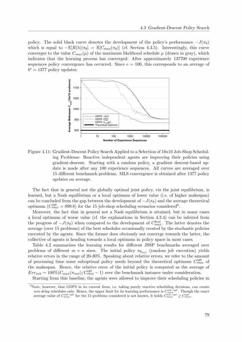
4.3 Gradient-Descent Policy Search
policy. The solid black curve denotes the development of the policy’s performance −J(πθ)which is equal to −E[R(h)|πθ] = E[Cmax(πθ)] (cf. Section 4.3.5). Interestingly, this curveconverges to the value Cmax(µ) of the maximum likelihood schedule µ (drawn in gray), whichindicates that the learning process has converged: After approximately 137700 experiencesequences policy convergence has occurred. Since e = 100, this corresponds to an average ofb? = 1377 policy updates.
Figure 4.11: Gradient-Descent Policy Search Applied to a Selection of 10x10 Job-Shop Schedul-ing Problems: Reactive independent agents are improving their policies usinggradient-descent. Starting with a random policy, a gradient descent-based up-date is made after any 100 experience sequences. All curves are averaged over15 different benchmark problems. MLS convergence is obtained after 1377 policyupdates on average.
The fact that in general not the globally optimal joint policy, viz the joint equilibrium, islearned, but a Nash equilibrium or a local optimum of lower value (i.e. of higher makespan)can be concluded from the gap between the development of −J(πθ) and the average theoreticaloptimum (Coptmax = 899.8) for the 15 job-shop scheduling scenarios considered9.
Moreover, the fact that in general not a Nash equilibrium is attained, but in many casesa local optimum of worse value (cf. the explanations in Section 4.3.4) can be inferred fromthe progress of −J(πθ) when compared to the development of Cbestmax. The latter denotes theaverage (over 15 problems) of the best schedules occasionally created by the stochastic policiesexecuted by the agents. Since the former does obviously not converge towards the latter, thecollective of agents is heading towards a local optimum in policy space in most cases.
Table 4.2 summarizes the learning results for different JSSP benchmarks averaged overproblems of different m × n sizes. The initial policy πθinit (random job execution) yieldsrelative errors in the range of 20-30%. Speaking about relative errors, we refer to the amountof processing time some suboptimal policy needs beyond the theoretical optimum Coptmax ofthe makespan. Hence, the relative error of the initial policy is computed as the average ofErrinit = 100%(Cmax(πinit)/C
optmax − 1) over the benchmark instance under consideration.
Starting from this baseline, the agents were allowed to improve their scheduling policies in
9Note, however, that GDPS in its current form, i.e. taking purely reactive scheduling decisions, can createnon-delay schedules only. Hence, the upper limit for its learning performance is Cnd−optmax . Though the exactaverage value of Cnd−optmax for the 15 problems considered is not known, it holds Cnd−optmax Coptmax.
79
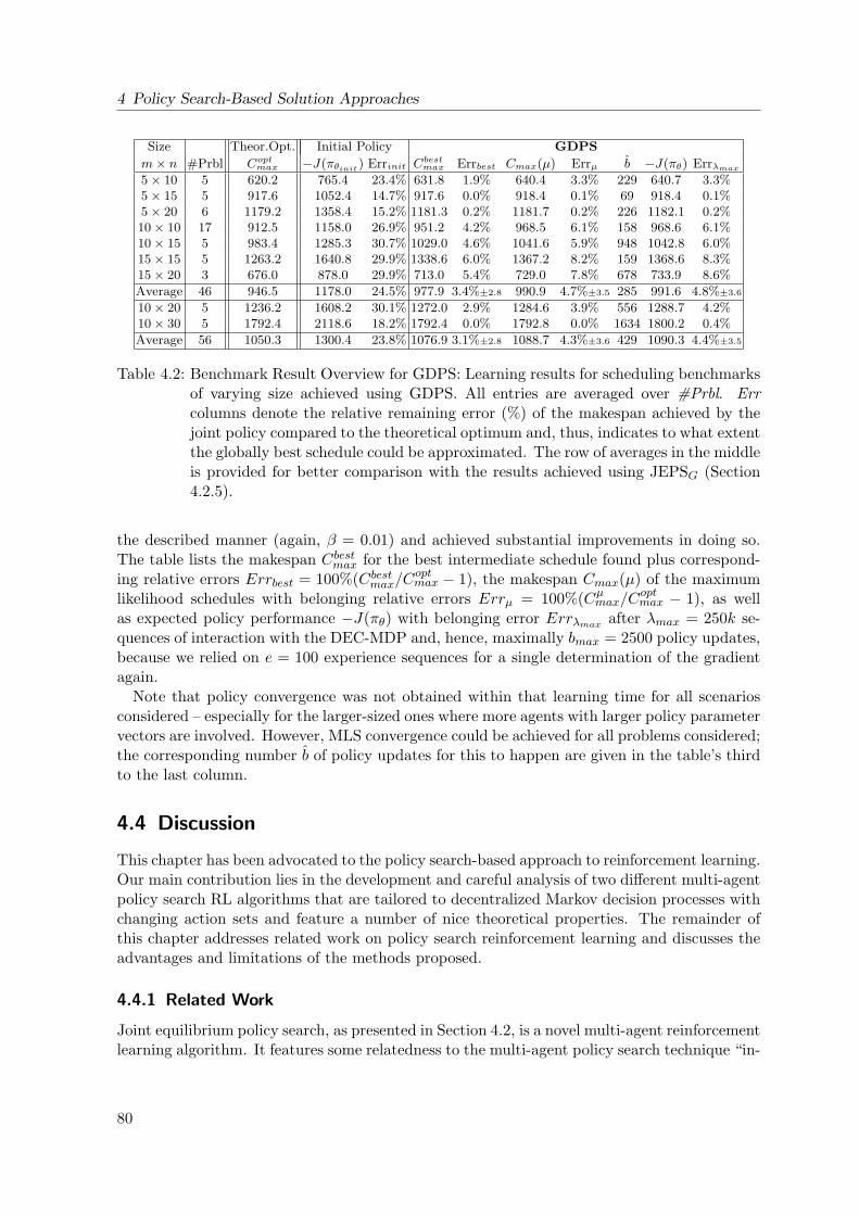
4 Policy Search-Based Solution Approaches
Size Theor.Opt. Initial Policy GDPS
m× n #Prbl Coptmax −J(πθinit) Errinit Cbestmax Errbest Cmax(µ) Errµ b −J(πθ) Errλmax
5× 10 5 620.2 765.4 23.4% 631.8 1.9% 640.4 3.3% 229 640.7 3.3%5× 15 5 917.6 1052.4 14.7% 917.6 0.0% 918.4 0.1% 69 918.4 0.1%5× 20 6 1179.2 1358.4 15.2% 1181.3 0.2% 1181.7 0.2% 226 1182.1 0.2%10× 10 17 912.5 1158.0 26.9% 951.2 4.2% 968.5 6.1% 158 968.6 6.1%10× 15 5 983.4 1285.3 30.7% 1029.0 4.6% 1041.6 5.9% 948 1042.8 6.0%15× 15 5 1263.2 1640.8 29.9% 1338.6 6.0% 1367.2 8.2% 159 1368.6 8.3%15× 20 3 676.0 878.0 29.9% 713.0 5.4% 729.0 7.8% 678 733.9 8.6%
Average 46 946.5 1178.0 24.5% 977.9 3.4%±2.8 990.9 4.7%±3.5 285 991.6 4.8%±3.6
10× 20 5 1236.2 1608.2 30.1% 1272.0 2.9% 1284.6 3.9% 556 1288.7 4.2%10× 30 5 1792.4 2118.6 18.2% 1792.4 0.0% 1792.8 0.0% 1634 1800.2 0.4%
Average 56 1050.3 1300.4 23.8% 1076.9 3.1%±2.8 1088.7 4.3%±3.6 429 1090.3 4.4%±3.5
Table 4.2: Benchmark Result Overview for GDPS: Learning results for scheduling benchmarksof varying size achieved using GDPS. All entries are averaged over #Prbl. Errcolumns denote the relative remaining error (%) of the makespan achieved by thejoint policy compared to the theoretical optimum and, thus, indicates to what extentthe globally best schedule could be approximated. The row of averages in the middleis provided for better comparison with the results achieved using JEPSG (Section4.2.5).
the described manner (again, β = 0.01) and achieved substantial improvements in doing so.The table lists the makespan Cbestmax for the best intermediate schedule found plus correspond-ing relative errors Errbest = 100%(Cbestmax/C
optmax − 1), the makespan Cmax(µ) of the maximum
likelihood schedules with belonging relative errors Errµ = 100%(Cµmax/Coptmax − 1), as well
as expected policy performance −J(πθ) with belonging error Errλmax after λmax = 250k se-quences of interaction with the DEC-MDP and, hence, maximally bmax = 2500 policy updates,because we relied on e = 100 experience sequences for a single determination of the gradientagain.
Note that policy convergence was not obtained within that learning time for all scenariosconsidered – especially for the larger-sized ones where more agents with larger policy parametervectors are involved. However, MLS convergence could be achieved for all problems considered;the corresponding number b of policy updates for this to happen are given in the table’s thirdto the last column.
4.4 Discussion
This chapter has been advocated to the policy search-based approach to reinforcement learning.Our main contribution lies in the development and careful analysis of two different multi-agentpolicy search RL algorithms that are tailored to decentralized Markov decision processes withchanging action sets and feature a number of nice theoretical properties. The remainder ofthis chapter addresses related work on policy search reinforcement learning and discusses theadvantages and limitations of the methods proposed.
4.4.1 Related Work
Joint equilibrium policy search, as presented in Section 4.2, is a novel multi-agent reinforcementlearning algorithm. It features some relatedness to the multi-agent policy search technique “in-
80
4.4 Discussion
cremental policy learning” (Fulda and Ventura, 2004). While the latter, however, is limitedto single-stage games, i.e. to stateless environments, JEPS consistently addresses sequentialdecision problems. In estimating the value of the joint equilibrium, JEPS follows a straight-forward approach of remembering the best global return obtained so far which is related tothe Rmax algorithm (Brafman and Tennenholtz, 2003) as well as to optimistic assumption Qlearning (Lauer and Riedmiller, 2000).
The utilization of policy gradient methods in the context of distributed problem solving isnot new. Building upon the statistical gradient-following policy learning scheme by Williams(1992), Peshkin et al. (2000) show that, when employing distributed control of factored actions,it is possible to find at least local optima in the space of the agents’ policies. While theseauthors evaluate their gradient-descent learning algorithm for a simulated soccer game, anotherprominent application domain targeted by several authors using PG approaches is the taskof network routing (Tao et al., 2001; Peshkin and Savova, 2002), which had previously beenexamined with the value function-based Q-Routing algorithm (Boyan and Littman, 1994). Incontrast to these pieces of work, the application of gradient-descent policy search to distributedproblems modelled as decentralized MDPs with changing action sets, and in particular for job-shop scheduling problems, as pursued in this thesis, is new.
Yagan and Tham (2007) study policy gradient methods for reinforcement learning agentsin the DEC-POMDP framework (Bernstein et al., 2002), as we do. In order to establishcoordination, they define a neighborhood of locally interacting agents which are allowed tofully exchange their local policies. By contrast, JEPS is explicitly geared towards learning joint(coordination) equilibria and GDPS, in the form proposed, regards inter-agent dependenciesonly implicitly. However, in Chapter 6 we will propose a mechanism for resolving transitiondependencies allowing agents to dedicatedly notify a single agent about a dependent actionthey have just taken and, in so doing, improve coordination. With regard to inter-agentcommunication, the idea of exploiting locality of interaction in distributed systems to optimizea global objective function had already been adopted in the context of dynamic constraintoptimization and satisfaction problems (e.g. Modi et al., 2005). Moreover, job-shop schedulingproblems have also been interpreted and solved as constraint optimization problems (e.g. Liuand Sycara, 1995) with the goal of finding an optimal solution through applying a sequence ofdistributed repair operations. In fact, such an approach bears some resemblance to the repair-based reinforcement learning approach to job-shop scheduling by Zhang and Dietterich (1995),but it is less related to our work since we interpret the scheduling task as a sequential decisionproblem. By contrast, of higher relevance to the GDPS approach is the work by Aberdeen andBuffet (2007) on PG methods for planning problems. Here, also a factorization of the globalpolicy is made and independently learning agents are employed for various temporal planningtasks.
4.4.2 Advantages and Limitations of JEPS and GDPS
Policy search methods have established as a reasonable alternative to value function-basedreinforcement learning methods. While the latter aim at estimating state-action values and,hence, consume an amount of memory that is proportional to the state space size, the formerfocus on the evaluation and direct optimization of the actor, i.e. the policy, as a whole.
In developing JEPS and GDPS, we have created two multi-agent policy search RL algo-rithms, that successfully tackle the fundamental problem of decentralized learning. Both algo-rithms exploit characteristics of DEC-MDPs with changing action sets and partially ordered
81
4 Policy Search-Based Solution Approaches
transition dependencies on their behalf. For instance, in parameterizing the agents’ policiesit suffices to utilize only one single parameter per local action, which gives rise to a compactpolicy representation: Each agent needs only a few parameters to represent its policy10 and,in so doing, severely restricts its space of representable policies.
All policies considered are stochastic ones which is of special advantage for partially observ-able domains for which it is well-known that the best deterministic policy can be arbitrarilyworse than the best stochastic one. Although each local state can be fully observed in theclass of DEC-MDPs we are concerned with, the global system state is hidden from any agentand, hence, can be observed in part only.
The empirical evaluation of JEPS as well as of GDPS has shown that both algorithms are wellsuited to acquire good approximate solutions, i.e. to learn joint policies of high quality. Appliedto job-shop scheduling problems, for many problem instances indeed optimal solutions arefound, for others near-optimal schedules with small relative errors with respect to the optimum.While JEPS in its basic version featured some problems (mainly due to too excessive memoryrequirements) when applied to larger-scale problems, JEPSG and GDPS performed well inlearning factored policies using independent agents and achieved comparable performance:On an identical problem set they reduced the relative error from an initial value (randompolicy) of about 24% to 6.6% ± 7.3 and 4.8% ± 3.6, respectively, which represents quite asuccessful result given the intricacy of the problems considered.
A highly appealing characteristic of the policy search procedures presented is that theyadhere to a number of interesting theoretical properties. On the one hand, for JEPSG we haveproved that it converges with probability one to the joint equilibrium indicated by the heuristicfunction it employs. On the other hand, GDPS is guaranteed to acquire a local optimum inthe space of factored multi-agent policies and, in fact, performs the same policy updates thata centralized gradient descent learner would carry out.
A limitation of the suggested methods in their current form is that we enabled them torealizing reactive policies only, implying that each agent never executes its idle action, if otheractions are available. In terms of scheduling problems, this means that at best non-delayschedules can be created and the optimal solution, which may be represented by a delayschedule (cf. Section 3.1.1), is possibly missed. In order to counteract this confinement, inChapter 6 we analyze two approaches that let the agents interacting with the DEC-MDPreason about their inter-agent dependencies and allow them to behave not purely reactively.These ideas can be easily integrated into the policy search reinforcement learning methodologypursued in this chapter and can be expected to expedite the performance of JEPS and GDPS.
Another limitation of JEPS is that it requires a deterministic environment, at least for theproposed version that relies on an accurate and deterministic determination of the maximalreturn. On the one hand, noisy immediate rewards render the current approach infeasible, asno longer a fixed value of the maximal return exists. On the other hand, if rewards are deter-ministic and only state transitions are probabilistic and, moreover, we assume the existence ofa heuristic function that is capable of noticing correctly whether a joint equilibrium has beenreached, JEPS is applicable for such a DEC-MDP. Although, in the context of this thesis, allexperimental evaluations focus on deterministic job-shop scheduling problems, GDPS is wellutilizable for stochastic ones as well and has been shown to bring about good results in thepresence of probabilistic durations of job operations (Gabel and Riedmiller, 2008b).
A vulnerability of both of our policy search methods is their dependency on learning-specific
10With the exception of the basic version of JEPS which employs a local, state-specific action parameterization.
82
4.4 Discussion
parameters. We have seen that JEPS may converge prematurely depending on its learningrate and, by contrast, a practical implementation of JEPSG can run into numerical underflowproblems when computing action probabilities. Likewise, the performance of GDPS is subjectto the accuracy of its gradient estimates – increasing which requires the agents to do moreinteraction with the environment – and subject to its learning rate. To this end, an adaptivemethod that modifies the learning rate as learning continues might bring about some relief;a successful combination of policy gradient reinforcement learning with the Rprop techniquefor realizing an adaptive learning rate has been suggested by (Riedmiller et al., 2007b). Apartfrom these points, GDPS is guaranteed to find local optima in the space of factored policiesand, hence, in general may attain neither a Nash equilibrium nor the optimal joint equilibrium.Additionally, the empirical results obtained in Sections 4.2.5 and 4.3.5 show that the difficultiesmentioned grow with the sizes of problems tackled.
A weakness of both policy search techniques discussed is the fact that they aim at distributedlearning of a joint policy for one specific problem. The acquired policy is, in general, of littleuse, if the task or the environment changes. Stated differently, the generalization capabilitiesof both JEPS and GDPS are poor. In terms of our application domain of scheduling one maysay that the presented policy search-based reinforcement learning algorithms are capable offinding very good schedules for individual problem instances, but that they do not supportthe reuse of the learned policies for different, though similar, scheduling problems. Therefore,in the following chapter, where value function-based reinforcement learning approaches moveinto the center of our interest, we will focus on the issue of generalization in more detail.
83

4 Policy Search-Based Solution Approaches
84
5 Value Function-Based Solution Approaches
In the previous chapter, we have focused on policy search-based reinforcement learning ap-proaches to tackle complex multi-agent problems. In spite of the mentioned intricacy of theclass of problems considered, we could show that reactive and independently learning agentscan be enabled to acquire near-optimal policies. The ability to learn from experience on atrial and error basis and with strongly limited state information denotes a challenge in itself,especially when compared to analytical solution methods that aim at finding a globally optimalpolicy in a centralized manner and with full information about the state of the world.
Another striking aspect, that goes beyond the idea of learning a solution instead of designingit, is however, to which extent the acquired joint policy is appropriate for different and similarproblems, i.e. the question how well does it perform in previously unseen situations. Thechapter at hand addresses the value function-based approach to reinforcement learning and,besides exploring the ability to perform distributed learning, focuses also on the mentionedissue of generalization performance.
We start by providing some foundations on value function-based RL in general, on theidea of batch-mode reinforcement learning, and on distributed approximative value functions.The main contribution of this chapter lies in Section 5.3 where we develop OA-NFQ, a data-efficient multi-agent RL algorithm for DEC-MDPs with changing action sets that is based onlearning agent-specific local value functions. Thereafter, we empirically evaluate all algorithmspresented in the context of distributed job-shop scheduling problems. We finish this chapterwith a discussion and point to related work.
5.1 Foundations
As pointed out, in reinforcement learning the purpose of the learning agent is formalized interms of a reward signal conveyed by the environment. More precisely, the agent’s goal is tomaximize the immediate rewards it perceives in the long run, which is denoted as the returnRt =
∑∞k=0 γ
tr(t + k). We have introduced the value V π(s) of a state s under policy π asthe expected return, when taking actions determined by π starting from s. Similarly, byQπ(s, a), which is defined as the expected return starting from state s by taking action a andfollowing π thereafter, we denote the value of the state-action pair (s, a). These types of values,i.e. state values as well as state-action values, and the corresponding value functions (V andQ) represent the central concept of value function-based reinforcement learning approaches.Besides, they take the role of the critic, when adopting the actor-critic view on reinforcementlearning systems as done in Section 2.1.3. And, as outlined in Section 2.1.5, learning optimalvalue functions constitutes the ultimate goal of the RL approaches we will be pursuing now.
5.1.1 The Issue of Generalization
In the previous chapter, we investigated actor-oriented policy search RL methods for multi-agent problems. In so doing, we exploited some properties of DEC-MDPs with changing sets,
85
5 Value Function-Based Solution Approaches
pre-eminently the fact that each agent can execute each action only once. This allowed usto make the agents learn, under certain convergence guarantees, high-quality policies whichbasically determine action execution orders: From the point of view of solving complex (at leastNP-hard) optimization tasks, such as job-shop scheduling problems, the algorithms derivedand empirical results obtained are convincing, especially when taking into account that adecentralized form of learning is taking place.
A natural question to ask then is, what happens if properties of the learning problem con-sidered are changed. For example, for some agent some action may be removed from Ari orthe order of an action’s execution over the agents as determined by dependency function σiis changed. Clearly, under such conditions the performance of the joint policies learned bythe policy search-based approaches explored in Chapter 4 will be impaired. In order for theknowledge acquired during learning to be of more general applicability it is no longer sufficientto describe local states si as sets of actions (si = α1, . . . , α|si|) and actions merely by someindex or label (e.g. label ‘x’ to denote some action αx from Ari ) which uniquely identifies itwithin an agent’s action set.
What is necessary instead, is a characterization of the properties of individual actions and,correspondingly, of sets of local actions (that is local states). Such a characterization oughtto be rich enough to reflect similarities and dissimilarities between actions with respect to theeffects their execution has. Hereby, it should rather represent properties of typical problemclasses instead of single problem instances, such that acquired knowledge is general and validfor similar problems as well. Moreover, it should be comprehensive in describing an agent’slocal situation and, hence, comprise features that exhibit some relation to the goal of learning.
Finally, we consider it important that the local policies which the agents learn independentlyare modest regarding their computational requirements: When it comes to their application tonew, previously unseen problem instances, we demand them to be executable under real-timeconditions, which means that we do not allot them arbitrary amounts of computation time.In terms of the job-shop scheduling application domain, hence, quick and reactive dispatchingdecisions must be taken by the agents, as opposed to the NP-hard complexity of predictive(centralized) scheduling techniques (cf. Section 3.3.1).
Although feature engineering, i.e. the accurate definition of appropriate state and actionfeatures, is not our primary concern, we provide some more details on that topic, with specialregard to JSSPs, in Section 5.4.1. Regardless of the specific feature definition, what we intendto do here has crucial implications: When addressing potentially the entire space of different,though similar problem instances of DEC-MDPs with changing action sets instead of a singleone, we likewise create an exponential increase in the size of the state (and action) spacesthe agents have to consider. Let us illustrate this issue with the help of an example from thejob-shop scheduling domain.
Example Consider the FT6 example that we introduced in Section 3.1 (Figure 3.1). Inter-preting this problem as a decentralized Markov decision process as proposed in Section 3.2.2,we face 6 agents each of which can execute |Ari | = 6 actions (corresponding to the operationsof the 6 jobs involved). Since Si = P(Ari ), this gives rise to |Si| = 26 = 64 local states forevery agent i and to an upper limit of |S| (26)6 = 236 for the joint state space. The latterinequation is strict, because the dependency graphs Gα of the problem which dictate that each
86
5.1 Foundations
action α can be available for maximally one agent at a time. Hence, it is easy to verify that
|S| ≤6∑
k=1
(6
6− k
)· 6k = 117648
is a tighter estimation of the joint state space’s size1. Therefore, for this single particularinstance it is easily possible to store all local states per agent or even (when adopting acentralized perspective) all joint states in a table, when intending to represent a value function.
IfO denotes the set of all operations in the FT6 problem (cf. Definition 3.1), then it obviouslyholds
maxδ(o)|o ∈ O = 10, (5.1)
i.e. the operations requiring most processing time need 10 time steps to be processed. Letus now consider the class of all job-shop scheduling problems definable that involve both sixjobs and resources without recirculation. Additionally, let us assume that each schedulingproblem instance J6×6 we regard adheres to Equation 5.1 as well. Then, this class of problemscomprises 1036 possible scheduling problems. Needless to say, that some kind of value functionapproximation mechanism is necessary already, if the learning agents shall cover (with theirvalue functions to be learned) a small fraction of the resulting 64 · 1036 possible local states.This argument is magnified in particular, if we address larger, more realistic problems thatinvolve more than only six jobs or resources.
In the context of this thesis, we will employ multi-layer perceptron (MLP) neural networksto represent value functions. On the one hand, feed-forward neural networks are known tobe capable of approximating arbitrarily closely any function f : D → R that is continuouson a bounded set D (Hornick et al., 1989). On the other hand, we aim at exploiting thenotoriously good generalization capabilities of neural networks and, hence, aim at yieldinggeneral dispatching policies, i.e. policies which are not just tuned for the situations encounteredduring training, but which are general enough to be applied to unknown situations, too.
5.1.2 Batch-Mode Reinforcement Learning
In Section 2.1.5, we have briefly outlined value iteration and Q learning as two basic rein-forcement learning algorithms. The associated updates to the state and state-action valuefunction according to Equation 2.4 and 2.5, respectively, are meant to be performed after eachsingle state transition experienced. This works well when reasonably small state or state-action spaces have to be considered such that the value function can be stored in tabular form.Interesting reinforcement learning problems, including the ones we are addressing, typicallyhave very large or even continuous state or state-action spaces which is why the use of valuefunction approximation mechanisms, as depicted in Section 5.1.1, is required.
In contrast to classic online reinforcement learning where updates to the value function aremade after each transition, batch-mode reinforcement learning methods store and reuse theirexperience which takes the shape of transition four-tuples. These tuples of experience consisteach of a state, and action taken in that state, the immediate reward received, as well asthe successor state entered. After having collected a batch, i.e. a larger number of transitiontuples, the computational update to the value function is performed.
1Note that, when assuming reactive agent behavior, which yields non-delay schedules, in fact only a fractionof those states can be reached.
87
5 Value Function-Based Solution Approaches
Batch-mode reinforcement learning has recently been successfully applied to various chal-lenging real-world applications (Riedmiller et al., 2007a; Csaji and Monostori, 2008; Deisenrothet al., 2008). Its popularity in general, and its particular advantages for the work at hand canbe attributed to various reasons:
• The reuse of stored experience renders batch-more reinforcement learning algorithmsparticularly data-efficient. This is of importance for real-world and, more generally, forlearning tasks where the amount of interaction with the environment shall be limited.
• When learning value functions in combination with a function approximator, the avail-ability of a batch of training data instead of single training patterns can be favorable indifferent respects. On the one hand, there seems to be no substantial gain, if a functionapproximator approximates the value function in a local way, like radial basis functionnetworks or instance- and case-based methods. However, even in that case batch-modetraining can yield improvements in terms of learning speed and performance (Gabel andRiedmiller, 2006a). On the other hand, many powerful function approximation schemesapproximate the target function in a global way (e.g. support vector regression, Gaussianprocesses, or multi-layer perceptrons). Here, changing the function value at one pointwith respect to a single training pattern may result in hard to predict changes at otherpoints in the space over which the function is spanned. To this end, it is of crucialimportance for the successful application of MLP nets as value function approximatorsin the context of reinforcement learning, that they are used embedded in a batch-modeRL algorithm where updates are performed based on a whole set of training patternssimultaneously.
• Apart from the batch-mode update that is beneficial when training global function ap-proximators in general, another advantage is that specifically for the training of MLPneural networks, advanced batch training methods, such as the Rprop training algo-rithm (Riedmiller and Braun, 1993), exist which have been shown to be more powerfuland parameter-insensitive than the gradient-descent method used commonly.
• Our main focus is on multi-agent reinforcement learning. Assuming independently learn-ing agents, we can conjecture that single transition tuples some agent experiences arestrongly affected by the actions taken concurrently by other agents. This dependency ofsingle transitions on external factors, i.e. on other agents’ policies, gives rise to anotherargument for batch training: While a single transition tuple contains probably too littleinformation for doing a reliable update, a rather comprehensive batch of experience maycontain sufficient information to apply value function-based RL also in a multi-agentcontext. We will investigate this issue in depth in Section 5.3.
Figure 5.1 sketches the general batch-mode reinforcement learning framework. It basicallyconsists of three main steps that are interconnected by two loops. The step of samplingexperience (outer loop) realizes interaction with the environment and creates a set of transitiontuples (data). The second step utilizes dynamic programming methods to generate a set oftraining patterns which are, subsequently and iteratively (inner loop), employed by some batchmode supervised learning algorithm that outputs an approximated function represented by thetraining patterns.
Note that most of the practical realizations of batch-mode reinforcement learning algorithmswork in alternating batch mode. This means that the outer loop can be iterated an arbitrary
88
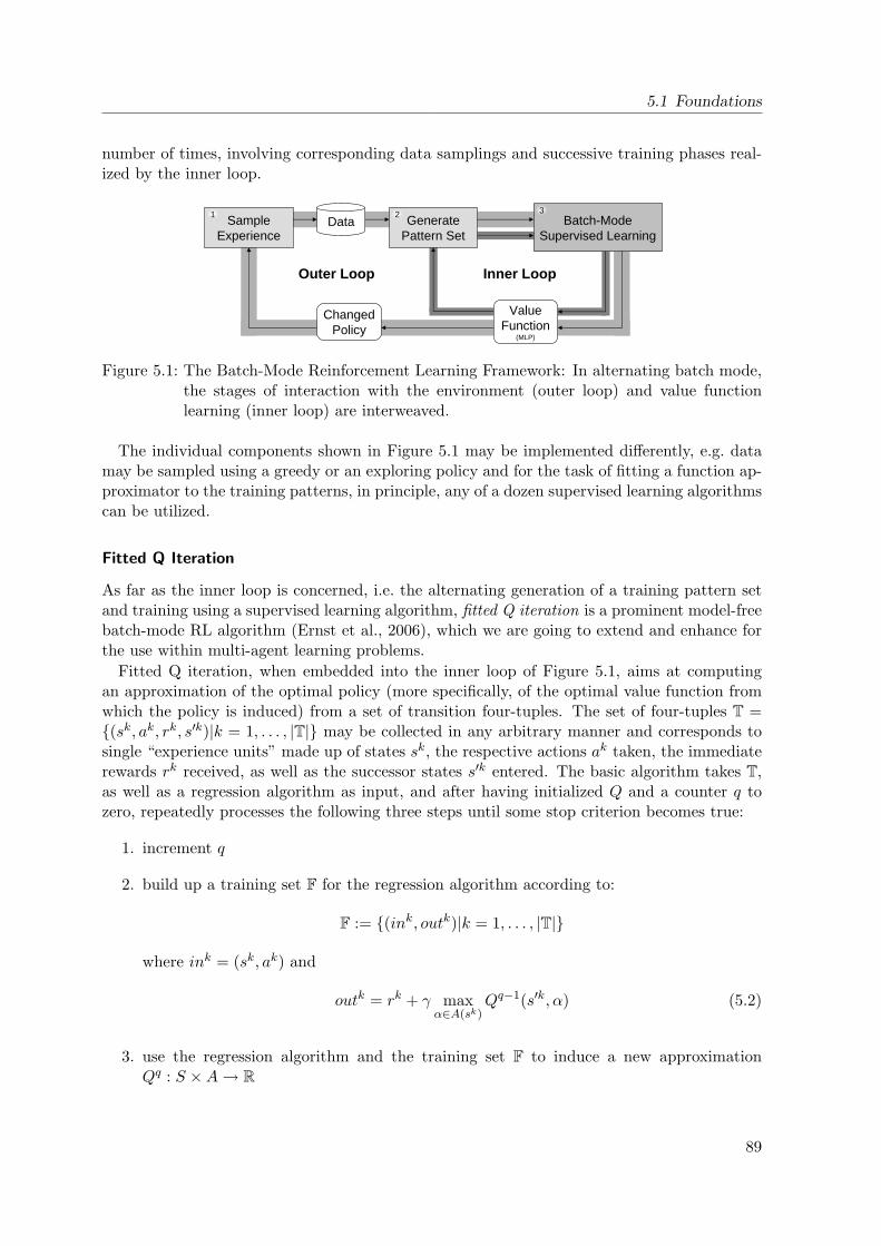
5.1 Foundations
number of times, involving corresponding data samplings and successive training phases real-ized by the inner loop.
SampleExperience
GeneratePattern Set
Batch-ModeSupervised Learning
Data
Inner LoopOuter Loop
ChangedPolicy
ValueFunction
(MLP)
1 2 3
Figure 5.1: The Batch-Mode Reinforcement Learning Framework: In alternating batch mode,the stages of interaction with the environment (outer loop) and value functionlearning (inner loop) are interweaved.
The individual components shown in Figure 5.1 may be implemented differently, e.g. datamay be sampled using a greedy or an exploring policy and for the task of fitting a function ap-proximator to the training patterns, in principle, any of a dozen supervised learning algorithmscan be utilized.
Fitted Q Iteration
As far as the inner loop is concerned, i.e. the alternating generation of a training pattern setand training using a supervised learning algorithm, fitted Q iteration is a prominent model-freebatch-mode RL algorithm (Ernst et al., 2006), which we are going to extend and enhance forthe use within multi-agent learning problems.
Fitted Q iteration, when embedded into the inner loop of Figure 5.1, aims at computingan approximation of the optimal policy (more specifically, of the optimal value function fromwhich the policy is induced) from a set of transition four-tuples. The set of four-tuples T =(sk, ak, rk, s′k)|k = 1, . . . , |T| may be collected in any arbitrary manner and corresponds tosingle “experience units” made up of states sk, the respective actions ak taken, the immediaterewards rk received, as well as the successor states s′k entered. The basic algorithm takes T,as well as a regression algorithm as input, and after having initialized Q and a counter q tozero, repeatedly processes the following three steps until some stop criterion becomes true:
1. increment q
2. build up a training set F for the regression algorithm according to:
F := (ink, outk)|k = 1, . . . , |T|
where ink = (sk, ak) and
outk = rk + γ maxα∈A(sk)
Qq−1(s′k, α) (5.2)
3. use the regression algorithm and the training set F to induce a new approximationQq : S ×A→ R
89
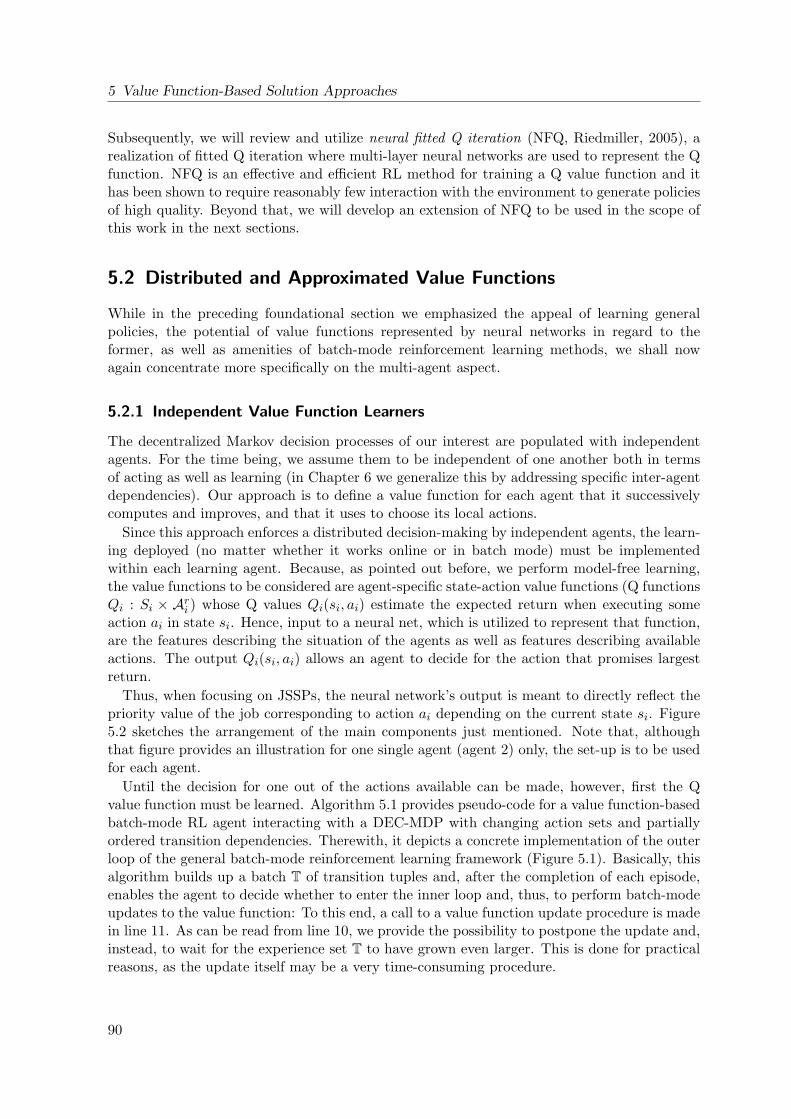
5 Value Function-Based Solution Approaches
Subsequently, we will review and utilize neural fitted Q iteration (NFQ, Riedmiller, 2005), arealization of fitted Q iteration where multi-layer neural networks are used to represent the Qfunction. NFQ is an effective and efficient RL method for training a Q value function and ithas been shown to require reasonably few interaction with the environment to generate policiesof high quality. Beyond that, we will develop an extension of NFQ to be used in the scope ofthis work in the next sections.
5.2 Distributed and Approximated Value Functions
While in the preceding foundational section we emphasized the appeal of learning generalpolicies, the potential of value functions represented by neural networks in regard to theformer, as well as amenities of batch-mode reinforcement learning methods, we shall nowagain concentrate more specifically on the multi-agent aspect.
5.2.1 Independent Value Function Learners
The decentralized Markov decision processes of our interest are populated with independentagents. For the time being, we assume them to be independent of one another both in termsof acting as well as learning (in Chapter 6 we generalize this by addressing specific inter-agentdependencies). Our approach is to define a value function for each agent that it successivelycomputes and improves, and that it uses to choose its local actions.
Since this approach enforces a distributed decision-making by independent agents, the learn-ing deployed (no matter whether it works online or in batch mode) must be implementedwithin each learning agent. Because, as pointed out before, we perform model-free learning,the value functions to be considered are agent-specific state-action value functions (Q functionsQi : Si × Ari ) whose Q values Qi(si, ai) estimate the expected return when executing someaction ai in state si. Hence, input to a neural net, which is utilized to represent that function,are the features describing the situation of the agents as well as features describing availableactions. The output Qi(si, ai) allows an agent to decide for the action that promises largestreturn.
Thus, when focusing on JSSPs, the neural network’s output is meant to directly reflect thepriority value of the job corresponding to action ai depending on the current state si. Figure5.2 sketches the arrangement of the main components just mentioned. Note that, althoughthat figure provides an illustration for one single agent (agent 2) only, the set-up is to be usedfor each agent.
Until the decision for one out of the actions available can be made, however, first the Qvalue function must be learned. Algorithm 5.1 provides pseudo-code for a value function-basedbatch-mode RL agent interacting with a DEC-MDP with changing action sets and partiallyordered transition dependencies. Therewith, it depicts a concrete implementation of the outerloop of the general batch-mode reinforcement learning framework (Figure 5.1). Basically, thisalgorithm builds up a batch T of transition tuples and, after the completion of each episode,enables the agent to decide whether to enter the inner loop and, thus, to perform batch-modeupdates to the value function: To this end, a call to a value function update procedure is madein line 11. As can be read from line 10, we provide the possibility to postpone the update and,instead, to wait for the experience set T to have grown even larger. This is done for practicalreasons, as the update itself may be a very time-consuming procedure.
90
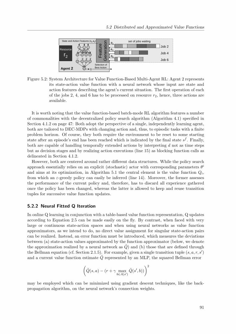
5.2 Distributed and Approximated Value Functions
Resource
r2
set of jobs waiting
Agent 2
Job 2
Job 4
Job 6
Fea
ture
Gen
erat
ionState and Action Features (sk,ak)
......
...
... ... ...... Selection of Best Action
Q
a2
a4
a6
Figure 5.2: System Architecture for Value Function-Based Multi-Agent RL: Agent 2 representsits state-action value function with a neural network whose input are state andaction features describing the agent’s current situation. The first operation of eachof the jobs 2, 4, and 6 has to be processed on resource r2, hence, three actions areavailable.
It is worth noting that the value function-based batch-mode RL algorithm features a numberof commonalities with the decentralized policy search algorithm (Algorithm 4.1) specified inSection 4.1.2 on page 47: Both adopt the perspective of a single, independently learning agent,both are tailored to DEC-MDPs with changing action and, thus, to episodic tasks with a finiteproblem horizon. Of course, they both require the environment to be reset to some startingstate after an episode’s end has been reached which is indicated by the final state sf . Finally,both are capable of handling temporally extended actions by interpreting d not as time stepsbut as decision stages and by realizing action executions (line 15) as blocking function calls asdelineated in Section 4.1.2.
However, both are centered around rather different data structures. While the policy searchapproach essentially relies on an explicit (stochastic) actor with corresponding parameters θi
and aims at its optimization, in Algorithm 5.1 the central element is the value function Qi,from which an ε-greedy policy can easily be inferred (line 14). Moreover, the former assessesthe performance of the current policy and, therefore, has to discard all experience gatheredonce the policy has been changed, whereas the latter is allowed to keep and reuse transitiontuples for successive value function updates.
5.2.2 Neural Fitted Q Iteration
In online Q learning in conjunction with a table-based value function representation, Q updatesaccording to Equation 2.5 can be made easily on the fly. By contrast, when faced with verylarge or continuous state-action spaces and when using neural networks as value functionapproximators, as we intend to do, no direct value assignment for singular state-action pairscan be realized. Instead, an error function must be introduced, which measures the deviationsbetween (a) state-action values approximated by the function approximator (below, we denotethe approximation realized by a neural network as Q) and (b) those that are defined throughthe Bellman equation (cf. Section 2.1.5). For example, given a single transition tuple (s, a, r, s′)and a current value function estimate Q represented by an MLP, the squared Bellman error(
Q(s, a)− (r + γ maxb∈A(s′)
Q(s′, b)))2
may be employed which can be minimized using gradient descent techniques, like the back-propagation algorithm, on the neural network’s connection weights.
91
5 Value Function-Based Solution Approaches
Input: value function Qi initialized randomly, exploration rate ε1: d← 0, T← ∅2: while not stop do3: observe si(d)4: if si(d) 6= ∅ or si(d) = sf then5: if d > 0 then6: receive immediate reward r(d− 1) //r(s(d-1),a(d-1),s(d))7: T← T ∪ (si(d− 1), α(d− 1), r(d− 1), si(d))8: endif9: if si(d) = sf then
10: if |T| is large enough then11: Qi ← call ValueFunctionUpdate(T) //batch-mode update12: d← 0 //do not flush experience set here13: else14: select α(d) ∈ si(d) by exploiting Qi greedily according to
α(d)← arg maxα∈si(d)Q(si(d), α)or a random α ∈ si(d) with probability ε
15: execute α(d)16: sσi(α(d)) ← sσi(α(d)) ∪ α(d) //influence local state of agent σi(α(d))17: si(d)← si(d) \ α(d)18: d← d+ 119: endif20: endif
Algorithm 5.1: Value Function-Based Batch-Mode RL from the Perspective of Agent i
A drawback of this type of online update is its wasteful utilization of data as each transitiontuple is used only once. As a consequence, typically thousands of episodes are necessary untila policy of sufficing quality is obtained (Riedmiller, 1999). This disadvantage can be tributed,at least in part, to the global approximation character of MLPs: Weight updates for a certainstate-action pair (s, a) may cause unforeseen changes of the value function in very differentregions of the joint state-action space.
Admittedly, the last-mentioned effect can be beneficial in terms of yielding generalization.However, recent studies on the neural fitted Q iteration (NFQ) algorithm, have shown thatmore stable and reliable learning results can be achieved when learning in batch-mode, whilenot sacrificing the excellent generalization capabilities of neural networks (Riedmiller, 2005).
As indicated, NFQ is an instance of the class of fitted Q iteration algorithms we describedabove, where the supervised batch-mode regression algorithm, i.e. the “fitting” part, is realizedby a multi-layer perceptron neural network. Let T = sk, ak, rk, s′k|k = 1, . . . ,T be a set oftransition 4-tuples and let Q denote the space of Q value functions over S×A representable byMLPs. Then, for each pattern k, NFQ calculates target values outk as specified in the contextof fitted Q iteration (cf. Equation 5.2), thereby utilizing the recent Q function estimate Q(q−1),and computes the next (qth) iterate of the state-action value function Qq by minimizing the
92
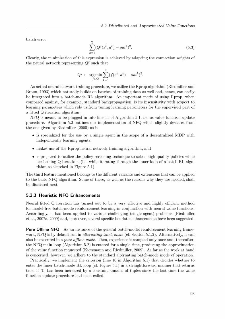
5.2 Distributed and Approximated Value Functions
batch errorT∑k=1
(Qq(sk, ak)− outk)2. (5.3)
Clearly, the minimization of this expression is achieved by adapting the connection weights ofthe neural network representing Qq such that
Qq ← arg minf∈Q
T∑k=1
(f(sk, ak)− outk)2.
As actual neural network training procedure, we utilize the Rprop algorithm (Riedmiller andBraun, 1993) which naturally builds on batches of training data as well and, hence, can easilybe integrated into a batch-mode RL algorithm. An important merit of using Rprop, whencompared against, for example, standard backpropagation, is its insensitivity with respect tolearning parameters which rids us from tuning learning parameters for the supervised part ofa fitted Q iteration algorithm.
NFQ is meant to be plugged in into line 11 of Algorithm 5.1, i.e. as value function updateprocedure. Algorithm 5.2 outlines our implementation of NFQ which slightly deviates fromthe one given by Riedmiller (2005) as it
• is specialized for the use by a single agent in the scope of a decentralized MDP withindependently learning agents,
• makes use of the Rprop neural network training algorithm, and
• is prepared to utilize the policy screening technique to select high-quality policies whileperforming Q iterations (i.e. while iterating through the inner loop of a batch RL algo-rithm as sketched in Figure 5.1).
The third feature mentioned belongs to the different variants and extensions that can be appliedto the basic NFQ algorithm. Some of these, as well as the reasons why they are needed, shallbe discussed next.
5.2.3 Heuristic NFQ Enhancements
Neural fitted Q iteration has turned out to be a very effective and highly efficient methodfor model-free batch-mode reinforcement learning in conjunction with neural value functions.Accordingly, it has been applied to various challenging (single-agent) problems (Riedmilleret al., 2007a, 2009) and, moreover, several specific heuristic enhancements have been suggested.
Pure Offline NFQ As an instance of the general batch-model reinforcement learning frame-work, NFQ is by default run in alternating batch mode (cf. Section 5.1.2). Alternatively, it canalso be executed in a pure offline mode. Then, experience is sampled only once and, thereafter,the NFQ main loop (Algorithm 5.2) is entered for a single time, producing the approximationof the value function requested (Kietzmann and Riedmiller, 2009). As far as the work at handis concerned, however, we adhere to the standard alternating batch-mode mode of operation.
Practically, we implement the criterion (line 10 in Algorithm 5.1) that decides whether toenter the inner batch-mode RL loop (cf. Figure 5.1) in a straightforward manner that returnstrue, if |T| has been increased by a constant amount of tuples since the last time the valuefunction update procedure had been called.
93
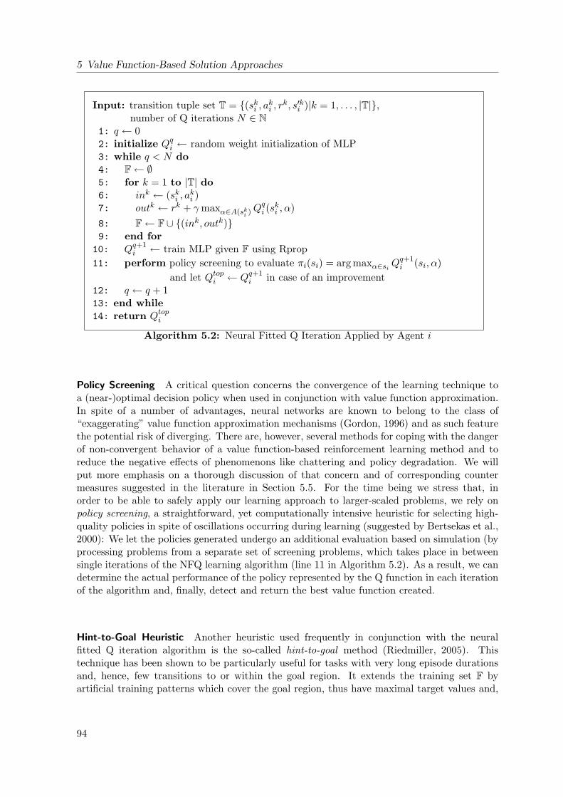
5 Value Function-Based Solution Approaches
Input: transition tuple set T = (ski , aki , rk, s′ki )|k = 1, . . . , |T|,number of Q iterations N ∈ N
1: q ← 02: initialize Qqi ← random weight initialization of MLP3: while q < N do4: F← ∅5: for k = 1 to |T| do6: ink ← (ski , a
ki )
7: outk ← rk + γmaxα∈A(ski )Qqi (s
ki , α)
8: F← F ∪ (ink, outk)9: end for
10: Qq+1i ← train MLP given F using Rprop
11: perform policy screening to evaluate πi(si) = arg maxα∈si Qq+1i (si, α)
and let Qtopi ← Qq+1i in case of an improvement
12: q ← q + 113: end while14: return Qtopi
Algorithm 5.2: Neural Fitted Q Iteration Applied by Agent i
Policy Screening A critical question concerns the convergence of the learning technique toa (near-)optimal decision policy when used in conjunction with value function approximation.In spite of a number of advantages, neural networks are known to belong to the class of“exaggerating” value function approximation mechanisms (Gordon, 1996) and as such featurethe potential risk of diverging. There are, however, several methods for coping with the dangerof non-convergent behavior of a value function-based reinforcement learning method and toreduce the negative effects of phenomenons like chattering and policy degradation. We willput more emphasis on a thorough discussion of that concern and of corresponding countermeasures suggested in the literature in Section 5.5. For the time being we stress that, inorder to be able to safely apply our learning approach to larger-scaled problems, we rely onpolicy screening, a straightforward, yet computationally intensive heuristic for selecting high-quality policies in spite of oscillations occurring during learning (suggested by Bertsekas et al.,2000): We let the policies generated undergo an additional evaluation based on simulation (byprocessing problems from a separate set of screening problems, which takes place in betweensingle iterations of the NFQ learning algorithm (line 11 in Algorithm 5.2). As a result, we candetermine the actual performance of the policy represented by the Q function in each iterationof the algorithm and, finally, detect and return the best value function created.
Hint-to-Goal Heuristic Another heuristic used frequently in conjunction with the neuralfitted Q iteration algorithm is the so-called hint-to-goal method (Riedmiller, 2005). Thistechnique has been shown to be particularly useful for tasks with very long episode durationsand, hence, few transitions to or within the goal region. It extends the training set F byartificial training patterns which cover the goal region, thus have maximal target values and,
94
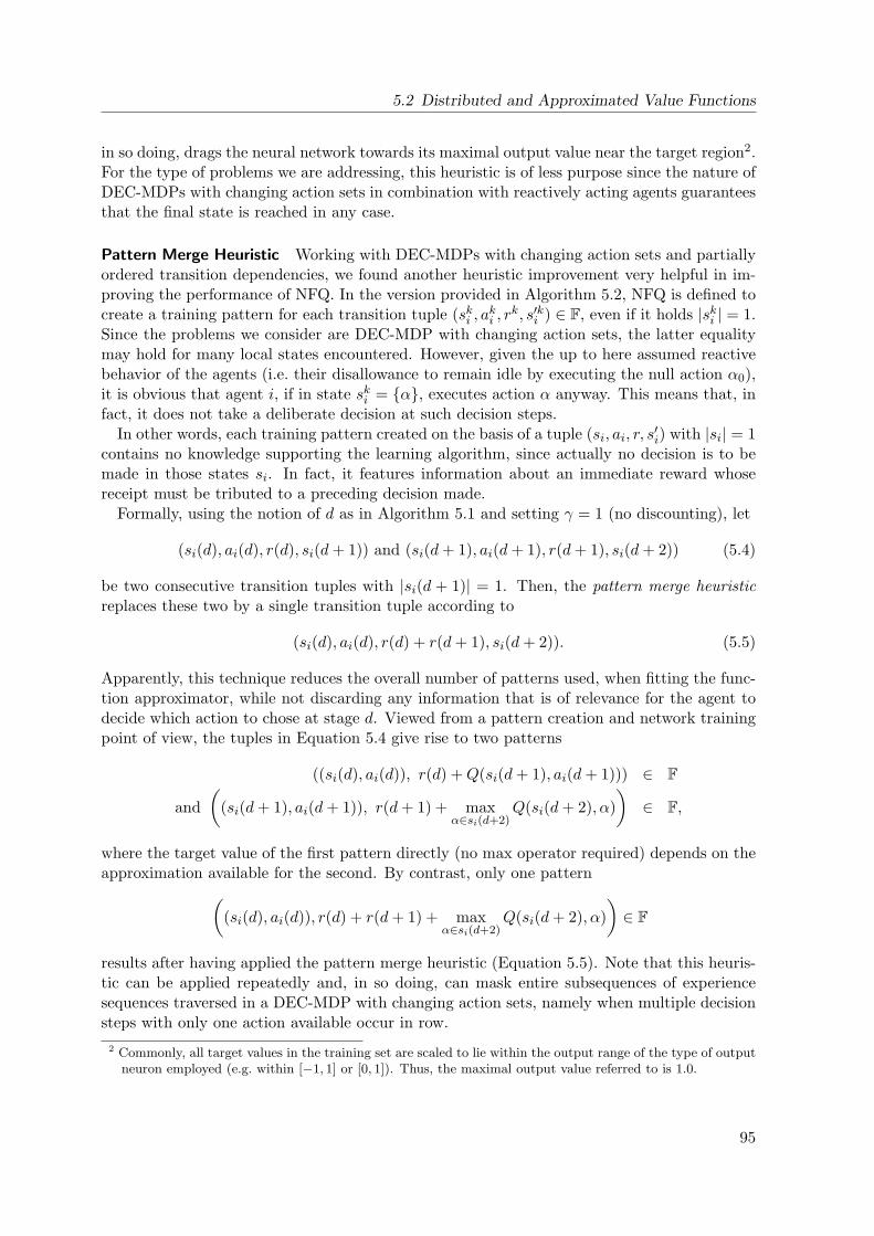
5.2 Distributed and Approximated Value Functions
in so doing, drags the neural network towards its maximal output value near the target region2.For the type of problems we are addressing, this heuristic is of less purpose since the nature ofDEC-MDPs with changing action sets in combination with reactively acting agents guaranteesthat the final state is reached in any case.
Pattern Merge Heuristic Working with DEC-MDPs with changing action sets and partiallyordered transition dependencies, we found another heuristic improvement very helpful in im-proving the performance of NFQ. In the version provided in Algorithm 5.2, NFQ is defined tocreate a training pattern for each transition tuple (ski , a
ki , r
k, s′ki ) ∈ F, even if it holds |ski | = 1.Since the problems we consider are DEC-MDP with changing action sets, the latter equalitymay hold for many local states encountered. However, given the up to here assumed reactivebehavior of the agents (i.e. their disallowance to remain idle by executing the null action α0),it is obvious that agent i, if in state ski = α, executes action α anyway. This means that, infact, it does not take a deliberate decision at such decision steps.
In other words, each training pattern created on the basis of a tuple (si, ai, r, s′i) with |si| = 1contains no knowledge supporting the learning algorithm, since actually no decision is to bemade in those states si. In fact, it features information about an immediate reward whosereceipt must be tributed to a preceding decision made.
Formally, using the notion of d as in Algorithm 5.1 and setting γ = 1 (no discounting), let
(si(d), ai(d), r(d), si(d+ 1)) and (si(d+ 1), ai(d+ 1), r(d+ 1), si(d+ 2)) (5.4)
be two consecutive transition tuples with |si(d + 1)| = 1. Then, the pattern merge heuristicreplaces these two by a single transition tuple according to
(si(d), ai(d), r(d) + r(d+ 1), si(d+ 2)). (5.5)
Apparently, this technique reduces the overall number of patterns used, when fitting the func-tion approximator, while not discarding any information that is of relevance for the agent todecide which action to chose at stage d. Viewed from a pattern creation and network trainingpoint of view, the tuples in Equation 5.4 give rise to two patterns
((si(d), ai(d)), r(d) +Q(si(d+ 1), ai(d+ 1))) ∈ F
and(
(si(d+ 1), ai(d+ 1)), r(d+ 1) + maxα∈si(d+2)
Q(si(d+ 2), α))∈ F,
where the target value of the first pattern directly (no max operator required) depends on theapproximation available for the second. By contrast, only one pattern(
(si(d), ai(d)), r(d) + r(d+ 1) + maxα∈si(d+2)
Q(si(d+ 2), α))∈ F
results after having applied the pattern merge heuristic (Equation 5.5). Note that this heuris-tic can be applied repeatedly and, in so doing, can mask entire subsequences of experiencesequences traversed in a DEC-MDP with changing action sets, namely when multiple decisionsteps with only one action available occur in row.
2 Commonly, all target values in the training set are scaled to lie within the output range of the type of outputneuron employed (e.g. within [−1, 1] or [0, 1]). Thus, the maximal output value referred to is 1.0.
95
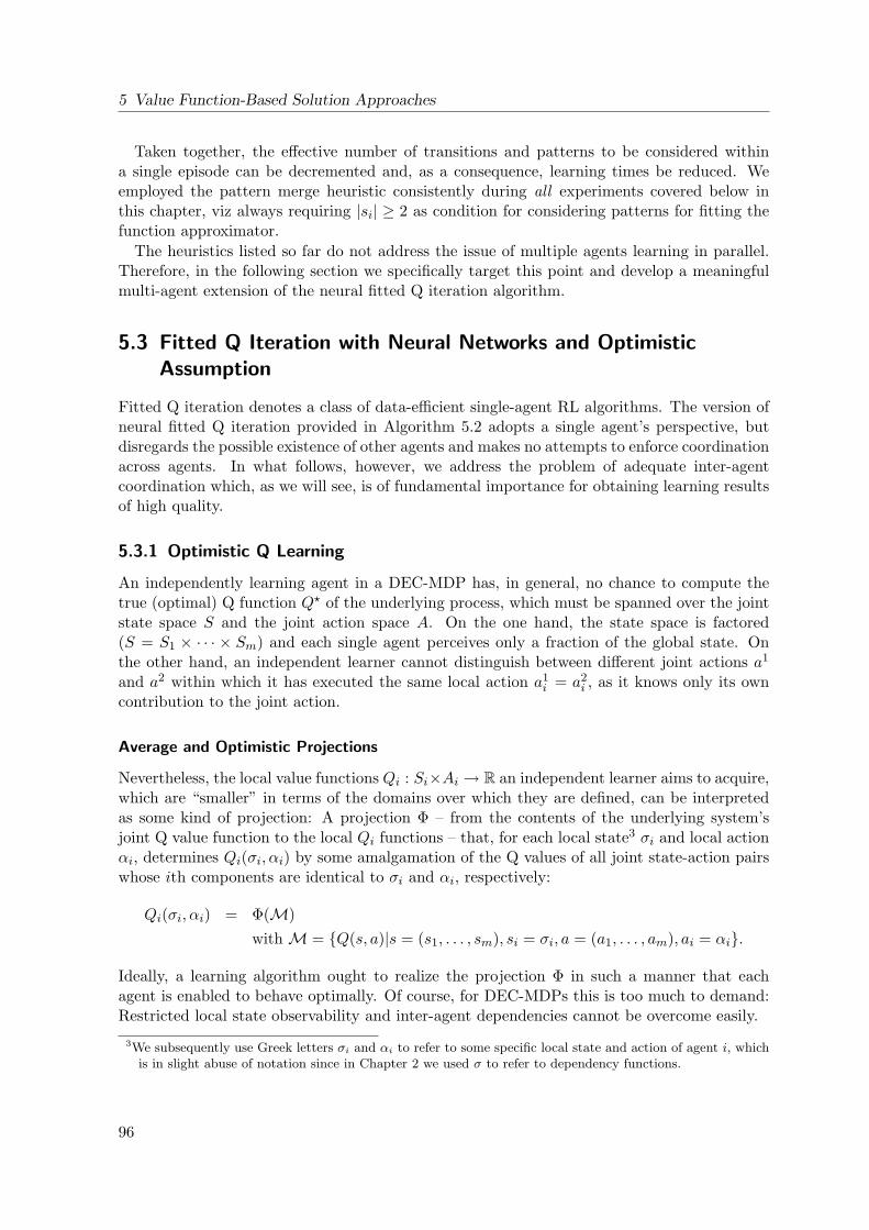
5 Value Function-Based Solution Approaches
Taken together, the effective number of transitions and patterns to be considered withina single episode can be decremented and, as a consequence, learning times be reduced. Weemployed the pattern merge heuristic consistently during all experiments covered below inthis chapter, viz always requiring |si| ≥ 2 as condition for considering patterns for fitting thefunction approximator.
The heuristics listed so far do not address the issue of multiple agents learning in parallel.Therefore, in the following section we specifically target this point and develop a meaningfulmulti-agent extension of the neural fitted Q iteration algorithm.
5.3 Fitted Q Iteration with Neural Networks and OptimisticAssumption
Fitted Q iteration denotes a class of data-efficient single-agent RL algorithms. The version ofneural fitted Q iteration provided in Algorithm 5.2 adopts a single agent’s perspective, butdisregards the possible existence of other agents and makes no attempts to enforce coordinationacross agents. In what follows, however, we address the problem of adequate inter-agentcoordination which, as we will see, is of fundamental importance for obtaining learning resultsof high quality.
5.3.1 Optimistic Q Learning
An independently learning agent in a DEC-MDP has, in general, no chance to compute thetrue (optimal) Q function Q? of the underlying process, which must be spanned over the jointstate space S and the joint action space A. On the one hand, the state space is factored(S = S1 × · · · × Sm) and each single agent perceives only a fraction of the global state. Onthe other hand, an independent learner cannot distinguish between different joint actions a1
and a2 within which it has executed the same local action a1i = a2
i , as it knows only its owncontribution to the joint action.
Average and Optimistic Projections
Nevertheless, the local value functions Qi : Si×Ai → R an independent learner aims to acquire,which are “smaller” in terms of the domains over which they are defined, can be interpretedas some kind of projection: A projection Φ – from the contents of the underlying system’sjoint Q value function to the local Qi functions – that, for each local state3 σi and local actionαi, determines Qi(σi, αi) by some amalgamation of the Q values of all joint state-action pairswhose ith components are identical to σi and αi, respectively:
Qi(σi, αi) = Φ(M)with M = Q(s, a)|s = (s1, . . . , sm), si = σi, a = (a1, . . . , am), ai = αi.
Ideally, a learning algorithm ought to realize the projection Φ in such a manner that eachagent is enabled to behave optimally. Of course, for DEC-MDPs this is too much to demand:Restricted local state observability and inter-agent dependencies cannot be overcome easily.
3We subsequently use Greek letters σi and αi to refer to some specific local state and action of agent i, whichis in slight abuse of notation since in Chapter 2 we used σ to refer to dependency functions.
96
5.3 Fitted Q Iteration with Neural Networks and Optimistic Assumption
However, for the class of deterministic multi-agent Markov decision processes (MMDPs,cf. Section 2.3.1), i.e. when assuming that each agent is capable of fully observing the globalsystem state, defining a projection which still yields optimal behavior is possible: Each agentthen makes assumptions concerning its teammates’ behaviors and, in so doing, compresses thecontents of the joint Q function by considering only those pieces of information which representthe assumed teammate behavior.
Let the joint state and action space be finite such that a corresponding value functioncould be represented using a simple value table and, hence, no value function approximationmechanism is used. When using Q learning in a distributed manner in an MMDP and withoutany further adaptations to the multi-agent setting, the individual Qi functions that are learnedby independently learning agents essentially represent a weighted average of joint state-actionentries that would have been stored in a global Q function, if a centralized (MDP-)perspectivewas adopted. Hence, after convergence of this kind of standard Q learning with its mildconvergence requirements (infinite number of updates for each state-action pair and properlydecaying learning rate), applied in an MMDP setting, it holds for all agents i ∈ Ag, for allglobal states s ∈ S, and for all local actions αi ∈ Ai
Qi(s, αi) =∑
a=(a1,...,am)ai=αi
(Pr(a|ai) ·
(∑s′∈S
p(s, a, s′) ·(r(s, a, s′) + γ max
β∈Ai(s′)Qi(s′, β)
)))(5.6)
where Pr(a|ai) denotes the probability that the joint action a is executed in state s whenagent i executes ai as its local action. Stated differently, in an MMDP with finite S and Ai forall i, the local value functions Qi represent the unique solution of the set of equations definedby 5.6.
Another more goal-oriented approach is to employ a so-called optimistic assumption regard-ing other agents’ action choices (Lauer and Riedmiller, 2000). Here, each agent assumes thatall other agents always act optimally, i.e. that the combination of all local actions forms anoptimal joint action vector. For the MMDP setting, the optimistic assumption Q update ruleis defined as
Qi(s, ai)← max Qi(s, ai), r(s, a, s′) + γ maxα∈Ai(s′)
Qi(s′, α) (5.7)
with current state s, action ai, successor state s′. Hence, the basic idea is that the expectedreturns of state-action pairs are captured in the value of Qi by successively taking the maxi-mum. This update rule (Equation 5.7) allows for learning distributed Q value functions givena deterministic environment and assuming that initially Qi ≡ 0 for all i and that the im-mediate rewards r(s, a, s′) are always larger or equal zero. For multi-agent systems with fullglobal state observability granted to each agent (MMDP setting) it can be shown (see Lauerand Riedmiller (2000) for a proof) that this optimistic assumption-based variant of Q learningproduces local state-action value functions whose best actions are the same as in centralizedQ learning, i.e. for all states s and local actions αi ∈ Ai it holds
Qi(s, αi) = maxa=(a1,...,am)
ai=αi
Q(s, a), (5.8)
provided that finite state-action spaces and deterministic state transitions and rewards aregiven. We also remark that Q learning with the optimistic update rule (Equation 5.7) within
97
5 Value Function-Based Solution Approaches
an MMDP setting yields a set of equations
Qi(s, αi) = maxa=(a1,...,am)
ai=αi
∑s′∈S
p(s, a, s′) ·(r(s, a, s′) + γ max
β∈Ai(s′)Qi(s′, β)
)
whose unique solution are the local state-action value functions Qi and, as proved by Lauerand Riedmiller (2000), for all Qi(s, αi) also Equation 5.8 holds.
We emphasize that, even for MMDPs, Equation 5.8 describes only a necessary, not a suffi-cient condition which enables the agents to choose optimal local actions. This point is striking,if different joint actions of equal value exist, i.e. if
∃s ∈ S, a = (a1, . . . , am) ∈ A(s), b = (b1, . . . , bm) ∈ A(s) : Q(s, a) = Q(s, b)and Q(s, a) ≥ Q(s, c) ∀c ∈ A(s).
Then it may happen, for example, that each agent, being unaware of other agents’ actionchoices, selects its local action according to
ai = arg maxα∈Ai(s)
Qi(s, α),
but that a = (a1, . . . , am) is different from a as well as from b and, consequently,
Q(s, a) maxc∈A(s)
Q(s, c).
Hence, the combination of all agents’ local actions is not optimal. This difficulty of coordinationamong agents (for MMDPs) can be overcome by keeping a separate data structure for the localpolicies πi, which is changed only, if during ongoing learning a true improvement in the localstate-action values has occurred: If for some state s ∈ S and local action ai ∈ Ai(s) a newvalue for Qi(s, ai) is computed that strictly dominates its previous value, then πi(s) is adapted(Lauer and Riedmiller, 2000).
For stochastic environments, optimistic assumption-based Q learning faces difficulties be-cause two different sources of uncertainty intermingle: Successor states and rewards are nolonger just co-influenced by the other agents’ behaviors, but also by the random disturbancescaused by the stochastic nature of the process. Both types of stochastic perturbations must behandled differently by the learning algorithm. While fluctuations due to other agents’ actionchoices ought to be considered in an optimistic manner (taking the maximum), noise shouldbe taken into account with respect to its expected value (cancelling it out).
As we intend to employ the optimistic assumption subsequently, we stick to deterministicenvironments during the agents’ learning phases. Note, however, that this requirement is nolonger necessary, when greedily exploiting the learned Q functions, i.e. when applying thecorresponding policies.
5.3.2 Optimism Under Partial State Observability
We now implement the step from systems with global state observability to systems with locallyfull, yet globally partial observable system states, i.e. the step from MMDPs to DEC-MDPs.
When calculating (table-based) state-action value functions Qi for agents within a DEC-MDP, these Qi functions must, for all local states σi ∈ Si and local actions αi ∈ Ai, adhere to
98
5.3 Fitted Q Iteration with Neural Networks and Optimistic Assumption
the following equation
Qi(σi, αi) =∑
s=(s1,...,sm)si=σi
Pr(s|si)∑
a=(a1,...,am)ai=αi
Pr(a|ai, si)∑s′∈S
s′=(s′1,...,s′m)
p(s, a, s′) · (r(s, a, s′) + γ maxβ∈Ai(s′i)
Qi(s′i, β)). (5.9)
Here, Pr(s|si) denotes the probability that the system is in state s when agent i finds itselfin local state si, Pr(a|ai, si) stands for the probability that the joint action a is executed bythe ensemble of agents while agent i executes action ai in si. Needless to say, that this set oflocal functions Qi obtained by applying standard Q learning in a distributed fashion – whichcan be interpreted as an average weighted projection from the central Q function to the localones – will in general contain information, whose greedy exploitation implements suboptimalbehavior.
Definition 5.1 (Optimistic Assumption-Based Q Learning for DEC-MDPs).Given the global state s = (s1, . . . , sm), a joint action a = (a1, . . . , am), and a successor states′ = (s′1, . . . , s
′m) of a factored m-agent DEC-MDP, optimistic assumption-based Q learning
performs for each agent i ∈ Ag and each decision stage d updates to the local agent-specific Qfunction Qi according to
Qi(si, ai)← max Qi(si, ai), r(s, a, s′) + γ maxβ∈Ai(s′i)
Qi(s′i, β) . (5.10)
Under the assumption of initializing Qi ≡ 0 for all i and requiring r(s, a, s′) ≥ 0 for alls, s′ ∈ S and a ∈ A, it is easy to see that the values of all Qi(si, ai) are non-decreasing.
For better differentiation, let us denote the local state-action value functions used in Equa-tion 5.10 by QDi (superscript D stands for the DEC-MDP setting) and the ones used inEquation 5.7 by QMi (here, superscript M indicates the MMDP setting). Then, it is easy toverify that
maxs=(s1,...,sm)
si=σi
QMi (s, αi) ≤ QDi (σi, αi) (5.11)
for all σi ∈ Si and all αi ∈ Ai(σi).Apparently, an optimistic assumption-based Q learning agent within DEC-MDPs assumes
that all other agents j were in local states sj whose combination s = (s1, . . . , sm) is of highvalue, given ai. In so doing, this method will in general overestimate the true value of localstate-action pairs (QDi ≥ QMi ). This may result in sub-optimal behavior, as non-optimal localactions may be assessed with a too high value estimate. So, the crucial question is how extremeis this overestimation? Or, stated differently, are there additional assumptions we can exploitto reduce the impact of that overestimation?
Discussion of the Optimistic Assumption Under Partial State Observability
While standard Q learning applied in a DEC-MDP yields average weighted local Q valuesaccording to Equation 5.9, applying the optimistic assumption according to Definition 5.1results in a set of equations whose unique solution are the local state-action value functionsQi : Si ×Ai with
QDi (σi, αi) = Qi(σi, αi) = maxs=(s1,...,sm)
si=σi
Pr(s|si) · maxa=(a1,...,am)
ai=αi
(r(s, a, s′) + γ max
β∈Ai(s′i)Qi(s′i, β)
)(5.12)
99
5 Value Function-Based Solution Approaches
for any σi ∈ Si and αi ∈ Ai(σi). For decentralized Markov decision processes with changingaction sets and partially ordered transition dependencies, the overestimation resulting fromthe maximum operator over states in Equation 5.11 and Equation 5.12 is limited due to severalreasons.
• In the course of simultaneous learning, other agents improve their policies as well, whichrepresents a universal argument in favor of the idea to assume that other agents behavein a beneficial way.
• Making an optimistic assumption with respect to the local states other agents are in(maxs,si=σi) is meaningful in that – if all agents behaved optimally – a trajectory withjoint states of high value is passed through (given a deterministic environment).
• Because local states are sets of locally available actions and since no action can beavailable for two different agents at the same time (due to the inter-agent dependenciesformalized by the dependency graphs Gα given in Definition 2.13), for the global states = (s1, . . . , sm) the constraint
∀j 6= i ∀sj : si ∩ sj = ∅holds, which severely restricts the number of joint states the system can be in. Accord-ingly, the maximum operators mentioned are to be evaluated only over subsets of thejoint state space S.
• When assuming reactive behavior by all agents (as we do here), local actions cannot beexecuted in any arbitrary order, but depending on availability. Consequently, each agentcan enter states only from a fraction of the set Si = P(Ai) and, hence, a fraction of thejoint state space S = S1 × · · · × Sm can be entered by the ensemble of agents.
For these reasons, optimistic assumption-based Q learning, when applied in the context ofthe special DEC-MDP settings we are interested in, is generally expected to be of superiorperformance when compared to the averaging made by standard Q learning (as implied byEquation 5.9), although both approaches feature identical worst case behavior. We next sug-gest a concrete algorithmic realization of a multi-agent reinforcement learning algorithm thatcombines the optimistic way of inter-agent coordination within a DEC-MDP setting with theneural batch-mode approach to reinforcement learning circumscribed in Section 5.2.2.
5.3.3 Batch-Mode Learning of Distributed Q Values
The straightforward utilization of NFQ as learning algorithm to be employed by each of theagents interacting with a DEC-MDP corresponds to the averaging projection described byEquation 5.9, though the sums are now defined no longer over the entire state space S oraction space A, but dependent on the states visited and actions executed as stored within thetransition tuple set T.
Recall that the focus in this work is on DEC-MDPs with changing action sets and partiallyordered transition dependencies, where Si = P(Ari ) and the set Ari of local actions is finite.During episode-based interaction with the environment (including resets to some initial stateafter episode endings are reached) it thus happens that an agent encounters some state repeat-edly within different episodes. Consequently, the batch of transition tuples the agent gathersmay contain multiple entries for certain state-action pairs (si, ai). This means, there may exist
100
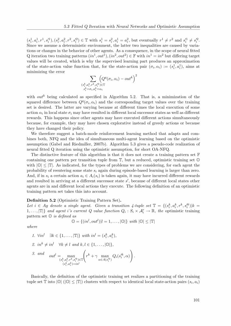
5.3 Fitted Q Iteration with Neural Networks and Optimistic Assumption
(s1i , a
1i , r
1, s′1i ), (s2i , a
2i , r
2, s′2i ) ∈ T with s1i = s2
i , a1i = a2
i , but eventually r1 6= r2 and s′1i 6= s′2i .Since we assume a deterministic environment, the latter two inequalities are caused by varia-tions or changes in the behavior of other agents. As a consequence, in the scope of neural fittedQ iteration two training patterns (in1, out1), (in2, out2) ∈ F with in1 = in2 but differing targetvalues will be created, which is why the supervised learning part produces an approximationof the state-action value function that, for the state-action pair (σi, αi) := (s1
i , a1i ), aims at
minimizing the error ∑(ski ,a
ki ,r
k,s′ki )∈Tski =σi,aki =αi
(Qq(σi, αi)− outk
)2
with outk being calculated as specified in Algorithm 5.2. That is, a minimization of thesquared difference between Qq(σi, αi) and the corresponding target values over the trainingset is desired. The latter are varying because at different times the local execution of someaction αi in local state σi may have resulted in different local successor states as well as differentrewards. This happens since other agents may have executed different actions simultaneouslybecause, for example, they may have chosen explorative instead of greedy actions or becausethey have changed their policy.
We therefore suggest a batch-mode reinforcement learning method that adapts and com-bines both, NFQ and the idea of simultaneous multi-agent learning based on the optimisticassumption (Gabel and Riedmiller, 2007b). Algorithm 5.3 gives a pseudo-code realization ofneural fitted Q iteration using the optimistic assumption, for short OA-NFQ.
The distinctive feature of this algorithm is that it does not create a training pattern set Fcontaining one pattern per transition tuple from T, but a reduced, optimistic training set Owith |O| ≤ |T|. As indicated, for the types of problems we are considering, for each agent theprobability of reentering some state si again during episode-based learning is larger than zero.And, if in si a certain action ai ∈ Ai(si) is taken again, it may have incurred different rewardsand resulted in arriving at a different successor state s′, because of different local states otheragents are in and different local actions they execute. The following definition of an optimistictraining pattern set takes this into account.
Definition 5.2 (Optimistic Training Pattern Set).Let i ∈ Ag denote a single agent. Given a transition 4-tuple set T = (ski , aki , rk, s′ki )|k =1, . . . , |T| and agent i’s current Q value function Qi : Si × Ari → R, the optimistic trainingpattern set O is defined as
O = (inl, outl)|l = 1, . . . , |O| with |O| ≤ |T|where
1. ∀inl ∃k ∈ 1, . . . , |T| with inl = (ski , aki ),
2. ink 6= inl ∀k 6= l and k, l ∈ 1, . . . , |O|,
3. andoutl = max
(ski ,aki ,r
k,s′ki )∈T(ski ,a
ki )=inl
(rk + γ max
α∈A(s′ki )Qi(s′ki , α)
).
Basically, the definition of the optimistic training set realizes a partitioning of the trainingtuple set T into |O| (|O| ≤ |T|) clusters with respect to identical local state-action pairs (si, ai)
101
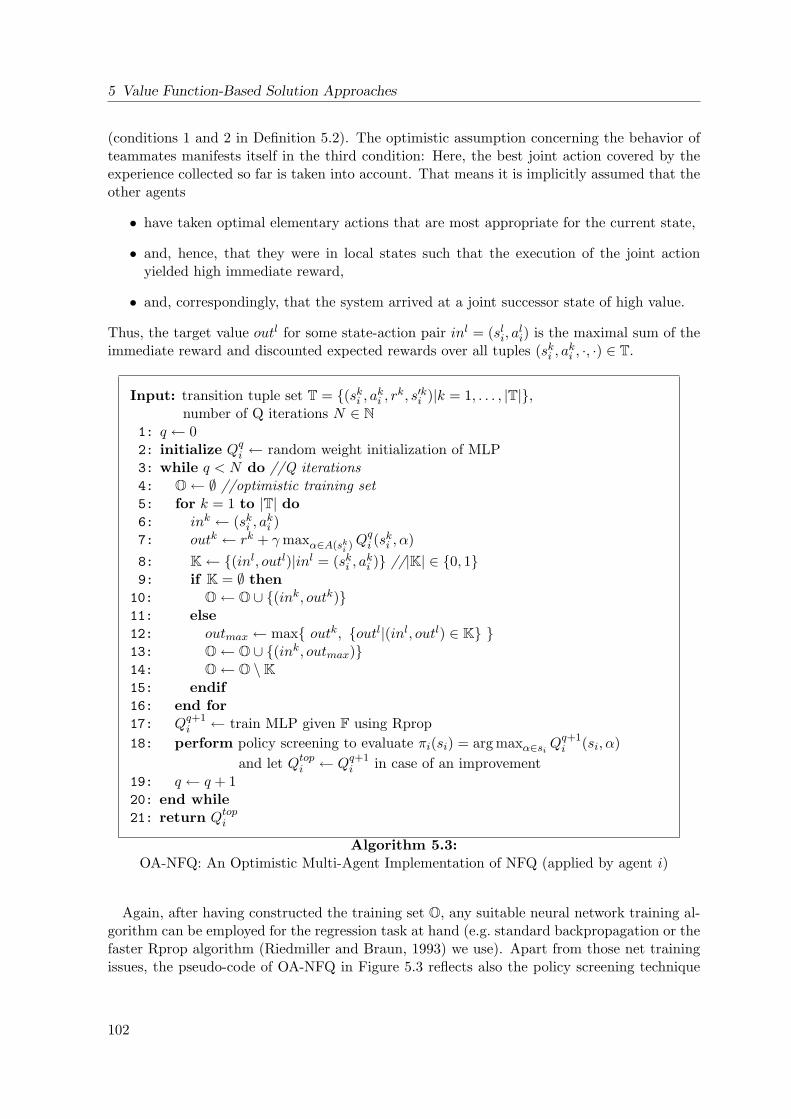
5 Value Function-Based Solution Approaches
(conditions 1 and 2 in Definition 5.2). The optimistic assumption concerning the behavior ofteammates manifests itself in the third condition: Here, the best joint action covered by theexperience collected so far is taken into account. That means it is implicitly assumed that theother agents
• have taken optimal elementary actions that are most appropriate for the current state,
• and, hence, that they were in local states such that the execution of the joint actionyielded high immediate reward,
• and, correspondingly, that the system arrived at a joint successor state of high value.
Thus, the target value outl for some state-action pair inl = (sli, ali) is the maximal sum of the
immediate reward and discounted expected rewards over all tuples (ski , aki , ·, ·) ∈ T.
Input: transition tuple set T = (ski , aki , rk, s′ki )|k = 1, . . . , |T|,number of Q iterations N ∈ N
1: q ← 02: initialize Qqi ← random weight initialization of MLP3: while q < N do //Q iterations4: O← ∅ //optimistic training set5: for k = 1 to |T| do6: ink ← (ski , a
ki )
7: outk ← rk + γmaxα∈A(ski )Qqi (s
ki , α)
8: K← (inl, outl)|inl = (ski , aki ) //|K| ∈ 0, 1
9: if K = ∅ then10: O← O ∪ (ink, outk)11: else12: outmax ← max outk, outl|(inl, outl) ∈ K 13: O← O ∪ (ink, outmax)14: O← O \K15: endif16: end for17: Qq+1
i ← train MLP given F using Rprop18: perform policy screening to evaluate πi(si) = arg maxα∈si Q
q+1i (si, α)
and let Qtopi ← Qq+1i in case of an improvement
19: q ← q + 120: end while21: return Qtopi
Algorithm 5.3:OA-NFQ: An Optimistic Multi-Agent Implementation of NFQ (applied by agent i)
Again, after having constructed the training set O, any suitable neural network training al-gorithm can be employed for the regression task at hand (e.g. standard backpropagation or thefaster Rprop algorithm (Riedmiller and Braun, 1993) we use). Apart from those net trainingissues, the pseudo-code of OA-NFQ in Figure 5.3 reflects also the policy screening technique
102
5.4 Empirical Evaluation
(cf. Section 5.2.3): In between individual Q iterations we let the current value function Qqiand the corresponding dispatching policy, respectively, undergo an additional evaluation basedon simulating a number of screening (scheduling) problems. Via that mechanism, the best Qiteration and its belonging Q function Qtopi is detected and finally returned.
We need to stress that in presence of using a neural value function approximation mechanismto represent Q and providing agents with local view information only, neither the convergenceguarantees for certain (averaging) types of fitted Q iteration algorithms (see Ernst et al. (2006)for a thorough discussion), nor the convergence proof of the optimistic assumption-based Qlearning algorithm (supporting finite state-action spaces, only) endure. Nevertheless, it ispossible to obtain impressive empirical results despite the approximations we employ, as wewill show in the next section.
5.4 Empirical Evaluation
In this section, we evaluate the use of approximate reinforcement learning for the job-shopscheduling benchmark problems that are in the center of our interest. In particular, we wantto address the question, if it is possible to utilize the algorithms we have described in thepreceding sections, to let the agents acquire high-quality dispatching policies for probleminstances of current standards of difficulty. Furthermore, we want to investigate, whether thelearned policies generalize to other, similar scheduling benchmark problems, too.
We begin by a comprehensive description of the experimental set-up we use and continue withsome results for two standard example benchmark problems. Then, we report on the learningresults for a broad collection of larger-sized benchmarks which also allows for a comparison tothe performance of policy search-based RL algorithms. Finally, we explore the generalizationcapabilities of OA-NFQ within two further experiments.
5.4.1 Experimental Set-Up
During all experiments to be described in the following, we employ value function-based rein-forcement learning to let the scheduling agents adapt their behavior policy, based on repeatedlycollecting experience within their environment and on receiving positive or negative feedback(reinforcement signals) from that environment, which, as before, we model as a decentralizedMarkov decision process with changing action sets. After that learning phase, each agent willhave obtained a purposive, reactive behavior for the respective environment. Then, during theapplication phase, e.g. during application in a real plant, each agent can make its schedulingdecisions very quickly by utilizing its reactive behavior (Gabel and Riedmiller, 2007c). Bothphases fit into the general batch-mode RL scheme outlined by Algorithm 5.1. During the latterphase, however, the learned Qi functions are exploited greedily by all agents. During the for-mer, by contrast, an exploration strategy is pursued which chooses random actions with someprobability and which makes updates to Qi using one of the value function update algorithmswe have presented (Algorithm 5.2 or 5.3).
Assuming a typical m × n job-shop scheduling problem modelled as a DEC-MDP withchanging action sets as well as reactively acting agents, it is clear that the transition graph ofthe system is acyclic and the number of states till reaching sf is finite. Therefore, all policiesare always proper and the problem horizon is finite, which is why the discount factor γ cansafely be set to one (no discounting).
103
5 Value Function-Based Solution Approaches
When considering a single job-shop problem, the number of possible states is, of course,finite. A focal point pursued in this chapter, however, is not to concentrate just on individualproblem instances, but on arbitrary ones. Hence, we assume the domain of state-action valuefunctions to be infinite or even continuous (see the discussion on that topic in Section 5.1.1),and employ multi-layer perceptron neural networks as function approximation mechanisms torepresent them. Each learning agent utilizes an MLP with one hidden layer (13:9:1 topology,cf. the illustration in Figure 5.2 and the following feature description) to represent its localstate-action value function Qi.
State and Action Features
When provided with some kind of a “global view” on the entire plant, i.e. when being grantedfull joint state observability, including information about the situation at all resources and theprocessing status of all jobs, a classical solution algorithm (like a branch-and-bound method)could be easily applied – even in parallel by each agent – to construct a disjunctive graph forthe problem at hand and solve it. In this respect, however, we have introduced a significantaggravation of the problem: First, we require a reactive scheduling decision in each state tobe taken in real-time, i.e. we do not allot arbitrary amounts of computation time. Second,the DEC-MDP-based problem interpretation restricts the amount of state information theagents get. Instead of the global view, each agent i has access to local state informationsi only, containing condensed information about its associated resource and the jobs waitingthere. On the one hand, this partial observability increases the difficulty in finding an optimalschedule. On the other hand, it allows for complete decentralization in decision-making, sinceeach agent is provided with information only that are relevant for making a local decision atthe resource it is responsible for. Apparently, this is particularly useful in applications whereno global control can be instantiated and where communication between distributed workingcenters is impossible (Gabel and Riedmiller, 2007a).
Nevertheless, the characterization of local states by means of several comprehensive features,viz the agents’ local view, is still large and forces us tackle a high-dimensional continuous state-action space:
Feature Vectors representing states si ∈ Si and actions (jobs4) ai ∈ Ari , as corresponding tothe resources’ local view, have to exhibit some relation to the expected rewards, henceto the makespan, and must allow for a comprehensive characterization of the currentsituation. Moreover, it is advisable to define features that represent properties of typicalproblem classes instead of single problem instances, so that the dispatching policiesacquired during learning are general and can be applied for different, though possiblysimilar scheduling problems, too. With respect to the desired real-time applicability ofthe system, the features should also be easy to compute, enabling a maximum degree ofreactivity. In the experiments whose results we describe in Section 5.4.3, we made use ofseven state features and six action features, thus having 13 inputs to the neural networkrepresenting the local state-action value function Qi.
State Features depict the current situation of the resource by describing its processing stateand the set si = α1, α2, . . . of jobs currently waiting at that resource. That job set
4Recall that we identify the set J of jobs in a job-shop scheduling problem J (Definition 3.1) with the setAr of all actions of a DEC-MDP with changing action sets and partially ordered transition dependencies(cf. Equation 3.1 in Section 3.2.2).
104
5.4 Empirical Evaluation
characterization includes the resource’s current workload, an estimation of the earliestpossible job completion times, and the estimated makespan. Furthermore, we capturecharacteristics of si by forming relations between minimal and maximal values of certainjob properties over the job set (like operation duration times or remaining job processingtimes).
Action Features characterize single jobs α from si currently selectable by i. Here, we aim atdescribing makespan-oriented properties of individual jobs (like processing time indices),as well as immediate consequences to be expected when processing that job next, viz theproperties of the job’s remaining operations (e.g. the relative remaining processing time).Apart from that, action features cover the significance of the next operation oα,k+1 ofjob α (e.g. its relative duration).
Local and Global Rewards
Throughout this work we consider cooperative agents. The cooperative nature of the DEC-MDPs we are addressing is expressed in the global reward signal all agents receive. Thus, thereward function r is used to specify the goal of the team of agents and is a function of states,joint actions, and successor states. As emphasized before, a desirable sequence of joint actionsought to correspond to a high long-term reward, which we formalized as the expected return(cf. Equation 2.1).
In principle, it is also possible to split the reward function into agent-specific components.Then, the global reward can be assembled by amalgamating local rewards that relate to singleagents. If this type of factorizing the reward is done in such a manner, that increasing anylocal reward yields also an increased global reward, too, then the system at hand is consideredto be reward independent (cf. Definition 2.11).
Our general specification of decentralized Markov decision processes with changing actionsets and partially ordered transition dependencies does not require any further preconditions orassumptions concerning the reward structure. When targeting job-shop scheduling problemswith the objective of minimizing maximum makespan of the resulting schedules, however, itis possible to express the global reward as a sum of local ones and, hence, to interpret thelearning system as a reward-independent one. The latter point is of interest insofar as it mayallow us to entirely decouple the learning agents: Instead of receiving local state observationsand taking local actions, the independent agents would then also receive only local rewards.Although this approach might be appealing from a practical point of view in terms of achievingpure decentralization, the selfish consideration of local reward signals only is expected to yieldless cooperative, and hence, sub-optimal joint performance.
The application of the general Q learning update rule, which also underlies the NFQ/OA-NFQ algorithms, establishes a relation between the local dispatching decisions as made byagent i and the overall optimization goal, since the global immediate rewards are taken intoconsideration. As an intuitive example in the realm of production scheduling, large negativeimmediate rewards (or, equivalently, high costs) may be caused due to tardy jobs, i.e. due totasks that were not accomplished until their deadline.
Another issue is that in job-shop scheduling, a resource is not allowed to take actions ateach discrete time step, after having started some operation oj,k the resource remains busyuntil that operation is finished. Therefore, we let Rsiai collect the immediate global rewards
105
5 Value Function-Based Solution Approaches
that arise between t and the next decision time point t+ δ(oj,k) of agent i according to
Rsiai(t,∆ti) =t+δ(oj,k)∑k=t
r(s(k), a(k), s(k + 1)).
If we assume convergence of Qi to the optimal local value function Q?i , we obtain a predictorof the expected accumulated global rewards that will arise, when in state si a job denoted byai would be processed next. Then, a policy π that exploits Qi greedily will lead to optimizedperformance of the scheduling agent. In accordance with our definitions of local policies fordecentralized MDPs (cf. Definition 2.9), a local, reactive, and deterministic policy that greedilyexploits its value function chooses its next local action as follows
π(si) = maxα∈Ai(si)
Qi(si, α).
Naturally, a crucial precondition for our value function-based RL approach to learning tomake sophisticated scheduling decisions is that the global immediate rewards (as feedback tothe learning agents) coincide with the overall objective of scheduling. We define the globalrewards r to be the sum of the rewards that can be associated with the agents (sum overi ∈ Ag) and jobs (sum over j ∈ J ):
r(s, a, s′) =m∑i=1
ui(s, a, s′) +n∑j=1
vj(s, a, s′). (5.13)
When focusing on minimizing overall tardiness, for instance, it is standing to reason to setui ≡ 0 and to let vj capture the tardiness Tj = max(0, cj − dj) of the jobs5 by
vj(s, a, s′) =−Tj , if j is being finished in state s′
0 , else(5.14)
A disadvantage of that formulation is that the cost function does not reflect when the tardi-ness actually occurs. Since that information may help the learning algorithm, the following,equivalent formulation is preferable, which assigns costs at each time step during processing:
vj(s, a, s′) =−1 , if j is tardy in state s′
0 , else(5.15)
Equations 5.14 and 5.15 are meant as an example and are no longer useful when the overallobjective is to minimize the makespan Cmax of the resulting schedule. Accordingly, informationabout tardy jobs or finishing times cj of individual jobs provide no meaningful indicator relatingto the makespan. There is, of course, a lot of work on tardiness-minimizing approaches (Gabeland Riedmiller, 2006b), but as far as the work at hand is considered we stick with aiming atminimizing makespan.
As emphasized in Section 3.2.2, it is known that the makespan of the schedule is minimized,if as many resources as possible are processing jobs concurrently and, accordingly, as few aspossible resources with queued jobs are in the system: A high utilization of the resourcesimplies a minimal makespan (Pinedo, 2002). Stated differently, the minimal makespan of a
5As defined in Chapter 3, cj refers to the completion time of job j. The deadline that may be associated withthat job is denoted by dj .
106

5.4 Empirical Evaluation
non-delay schedule is obtained when the number of time steps can be minimized during whichjobs are waiting for processing at the resources’ queues. This argument gives rise to setting
vj ≡ 0 andui(s, a, s′) = −|j | j queued at i| (5.16)
so that high negative rewards are generated when many jobs, that are waiting for furtherprocessing, are in the system and, hence, the overall utilization of the resources is poor.
Our definition of global immediate rewards in Equation 5.13 does in general not supportreward independence according to Definition 2.11. However, it is worth noting that – for theobjective of minimizing maximum makespan we are interested in – the reward formulationgiven by Equation 5.16 in fact yields reward independence. Although each function ui (for alli ∈ Ag) is defined over S ×A× S, it actually requires information relating to the situation ofagent i only and, accordingly, we can define local reward functions ri : Si ×Ai × Si as
ri(σ, α, σ′) = ui(s, a, s′) ∀σ, σ′ ∈ Si, α ∈ Ai and∃s = (s1, . . . , sm), a = (a1, . . . , am), s′ = (s′1, . . . , s
′m) : si = σ, ai = α, s′i = σ′.
This in turn allows us to interpret the global reward r as a sum of local rewards ri by
r(s, a, s′) =m∑i=1
ri(si, ai, s′i)
for all s = (s1, . . . , sm), a = (a1, . . . , am) ,s′ = (s′1, . . . , s′m) as demanded in the definition of
reward independence (Definition 2.11).The important point to be noted about the idea to make each agent learn based purely
on local rewards ri(si, ai, s′i) = −|j | j queued at i| is that this in fact recasts the learningobjective from reducing the length of the schedule (i.e. makespan) to minimizing the numberof jobs waiting at any resource individually. The latter, however, is in conformity with theutilization of the SPT dispatching rule discussed in Section 3.3.2, which always selects thatjob whose next operation has the shortest processing time. Generally speaking, the SPT ruleis one of the rather well-performing dispatching rules, if the goal is to minimize makespan: Formany scheduling benchmark problems it yields satisfying or good values of Cmax, but as it isa very simple and static heuristic, it may also fail on certain problem instances. This is, forexample, the case for the small educational benchmark problem FT6, where in fact the worstperformance possible is brought about, if all agents involved make their decisions based on theSPT dispatching rule (CSPTmax = 88, cf. Figure 4.8).
As pointed out, our main focus is on conveying a global reward signal to the independentlylearning agents, but in the next section we also briefly examine the performance loss yielded,when agents receive local rewards only and, thus, learn purely selfishly.
5.4.2 Example Benchmarks
Similarly as in the chapter on policy search-based reinforcement learning, we start our empir-ical analysis with the educational benchmark problem FT6 presented in Section 3.1.1. Duringthe data collection stage of our batch-mode reinforcement learning approach, each agent exe-cutes an ε-greedy, reactive, deterministic policy (ε = 0.2) derived from its current Q function.For the problem instances at hand, the value function update procedure (line 11 of Algorithm
107
5 Value Function-Based Solution Approaches
5.1) is entered each time an agent has extended its set of transition 4-tuples by 50 additionalexperience units. As far as the fitted Q iteration part is concerned, we use N = 20 Q itera-tions throughout all our experiments. And, concerning the supervised learning part involved,we employed the Rprop neural network training procedure with 500 epochs and its defaultparameter settings (η+ = 1.2, η− = 0.5).
In principle, we distinguish between three different modes of operation for the learningagents.
• During the learning phase – which we might also call experience collection and processingphase –, a set SL of scheduling problem instances is repeatedly processed on the simulatedplant, where the agents associated to the m resources follow their ε-greedy policies,sample experience, and at times adapt their policies. This corresponds to the outer loopof the batch-mode reinforcement learning framework sketched in Figure 5.1.
• When adapting their behavior policies using one of the value function update algorithmsdiscussed (in the context of fitted Q iteration, cf. the inner loop within Figure 5.1), theagents may utilize the policy screening technique outlined in Section 5.2.3. In that case,they process scheduling scenarios from a separate screening set SS for validation in orderto assess the quality of greedy policies induced from intermediately created state-actionvalue functions.
• During the evaluation or application phase, the ensemble of agents processes schedulingbenchmark instances from a set SA of test problems, employing greedy policies withrespect to the local value functions learned.
As far as the example benchmarks are concerned we address next, we let SL = SS = SA,thus making the agents learn to make good dispatching decisions for specific problem instanceswithout addressing the issue of generalization.
FT6 Benchmark Table 5.1 summarizes the average makespan values plus corresponding stan-dard deviations, when using value function-based batch-mode reinforcement learning agentsfor the FT6 benchmark. A first observation to be made is that local reward signals indeedmake the agents generate selfish behavior which mimics the SPT dispatching priority rule.This effect is most apparent in the table’s first row for the OA-NFQ algorithm where maximalmakespan (86.17) is attained, very much approaching the performance of SPT (88.0).
Using the policy screening technique in conjunction with local rewards (second row of Ta-ble 5.1) represents a somewhat inconsistent course of action: On the one hand, local rewardsreinforce SPT-like behavior and, hence, a policy yielding high makespan values. On the otherhand, policy screening analyzes the N = 20 value functions and corresponding policies gen-erated during the Q iteration process and picks the one with minimal makespan. Needless tosay that this contradictory combination of learning goals is, in particular for the FT6 problem,inappropriate and generally yields policies that create average makespan schedules.
Let us more specifically focus on the case of global rewards. If no policy screening is con-ducted and, hence, the Q value function after the 20th fitted Q iteration is considered, OA-NFQis only marginally superior to NFQ. The performance achievable in this setting (third row inthe result table) features a rather high standard deviation and is inferior to, for example, thegradient-descent policy search algorithms investigated in Section 4.3. This fact points to apotential weakness of the neural value function-based batch-mode learning approach and thus
108
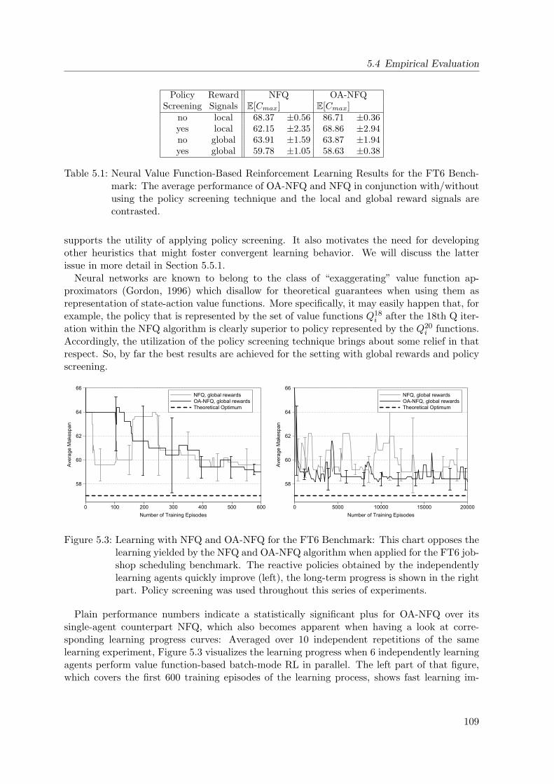
5.4 Empirical Evaluation
Policy Reward NFQ OA-NFQScreening Signals E[Cmax] E[Cmax]
no local 68.37 ±0.56 86.71 ±0.36yes local 62.15 ±2.35 68.86 ±2.94no global 63.91 ±1.59 63.87 ±1.94yes global 59.78 ±1.05 58.63 ±0.38
Table 5.1: Neural Value Function-Based Reinforcement Learning Results for the FT6 Bench-mark: The average performance of OA-NFQ and NFQ in conjunction with/withoutusing the policy screening technique and the local and global reward signals arecontrasted.
supports the utility of applying policy screening. It also motivates the need for developingother heuristics that might foster convergent learning behavior. We will discuss the latterissue in more detail in Section 5.5.1.
Neural networks are known to belong to the class of “exaggerating” value function ap-proximators (Gordon, 1996) which disallow for theoretical guarantees when using them asrepresentation of state-action value functions. More specifically, it may easily happen that, forexample, the policy that is represented by the set of value functions Q18
i after the 18th Q iter-ation within the NFQ algorithm is clearly superior to policy represented by the Q20
i functions.Accordingly, the utilization of the policy screening technique brings about some relief in thatrespect. So, by far the best results are achieved for the setting with global rewards and policyscreening.
Figure 5.3: Learning with NFQ and OA-NFQ for the FT6 Benchmark: This chart opposes thelearning yielded by the NFQ and OA-NFQ algorithm when applied for the FT6 job-shop scheduling benchmark. The reactive policies obtained by the independentlylearning agents quickly improve (left), the long-term progress is shown in the rightpart. Policy screening was used throughout this series of experiments.
Plain performance numbers indicate a statistically significant plus for OA-NFQ over itssingle-agent counterpart NFQ, which also becomes apparent when having a look at corre-sponding learning progress curves: Averaged over 10 independent repetitions of the samelearning experiment, Figure 5.3 visualizes the learning progress when 6 independently learningagents perform value function-based batch-mode RL in parallel. The left part of that figure,which covers the first 600 training episodes of the learning process, shows fast learning im-
109
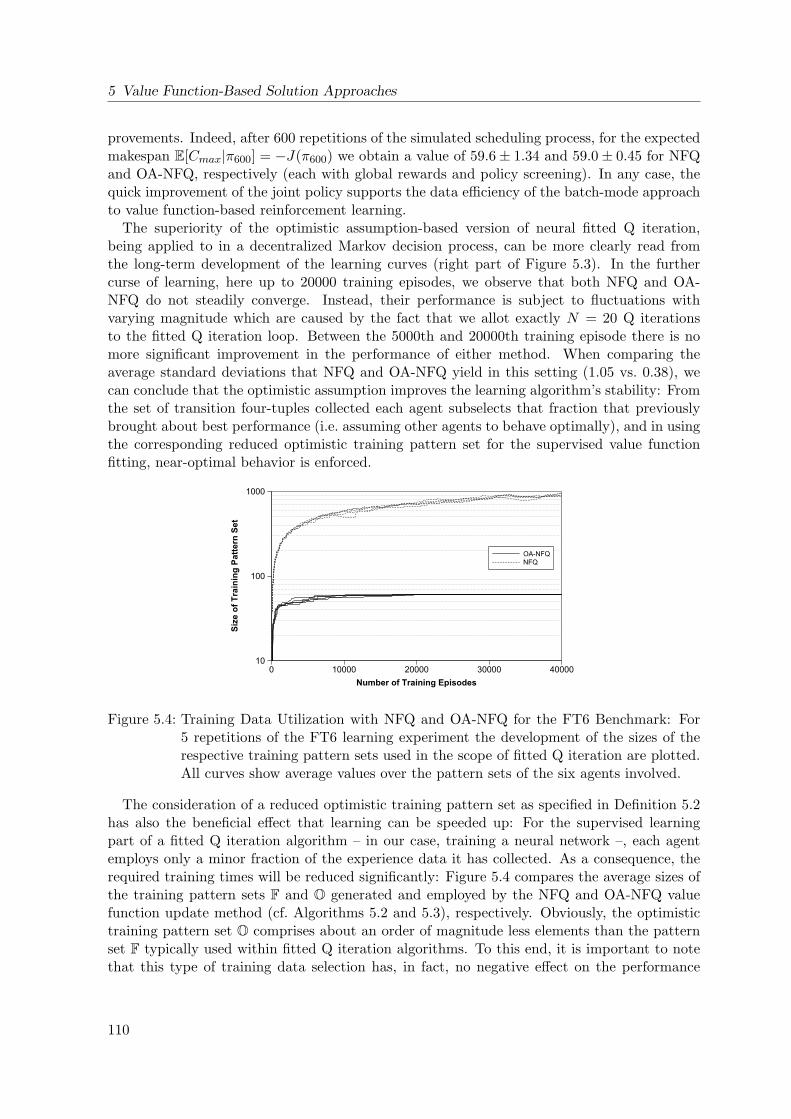
5 Value Function-Based Solution Approaches
provements. Indeed, after 600 repetitions of the simulated scheduling process, for the expectedmakespan E[Cmax|π600] = −J(π600) we obtain a value of 59.6± 1.34 and 59.0± 0.45 for NFQand OA-NFQ, respectively (each with global rewards and policy screening). In any case, thequick improvement of the joint policy supports the data efficiency of the batch-mode approachto value function-based reinforcement learning.
The superiority of the optimistic assumption-based version of neural fitted Q iteration,being applied to in a decentralized Markov decision process, can be more clearly read fromthe long-term development of the learning curves (right part of Figure 5.3). In the furthercurse of learning, here up to 20000 training episodes, we observe that both NFQ and OA-NFQ do not steadily converge. Instead, their performance is subject to fluctuations withvarying magnitude which are caused by the fact that we allot exactly N = 20 Q iterationsto the fitted Q iteration loop. Between the 5000th and 20000th training episode there is nomore significant improvement in the performance of either method. When comparing theaverage standard deviations that NFQ and OA-NFQ yield in this setting (1.05 vs. 0.38), wecan conclude that the optimistic assumption improves the learning algorithm’s stability: Fromthe set of transition four-tuples collected each agent subselects that fraction that previouslybrought about best performance (i.e. assuming other agents to behave optimally), and in usingthe corresponding reduced optimistic training pattern set for the supervised value functionfitting, near-optimal behavior is enforced.
Figure 5.4: Training Data Utilization with NFQ and OA-NFQ for the FT6 Benchmark: For5 repetitions of the FT6 learning experiment the development of the sizes of therespective training pattern sets used in the scope of fitted Q iteration are plotted.All curves show average values over the pattern sets of the six agents involved.
The consideration of a reduced optimistic training pattern set as specified in Definition 5.2has also the beneficial effect that learning can be speeded up: For the supervised learningpart of a fitted Q iteration algorithm – in our case, training a neural network –, each agentemploys only a minor fraction of the experience data it has collected. As a consequence, therequired training times will be reduced significantly: Figure 5.4 compares the average sizes ofthe training pattern sets F and O generated and employed by the NFQ and OA-NFQ valuefunction update method (cf. Algorithms 5.2 and 5.3), respectively. Obviously, the optimistictraining pattern set O comprises about an order of magnitude less elements than the patternset F typically used within fitted Q iteration algorithms. To this end, it is important to notethat this type of training data selection has, in fact, no negative effect on the performance
110
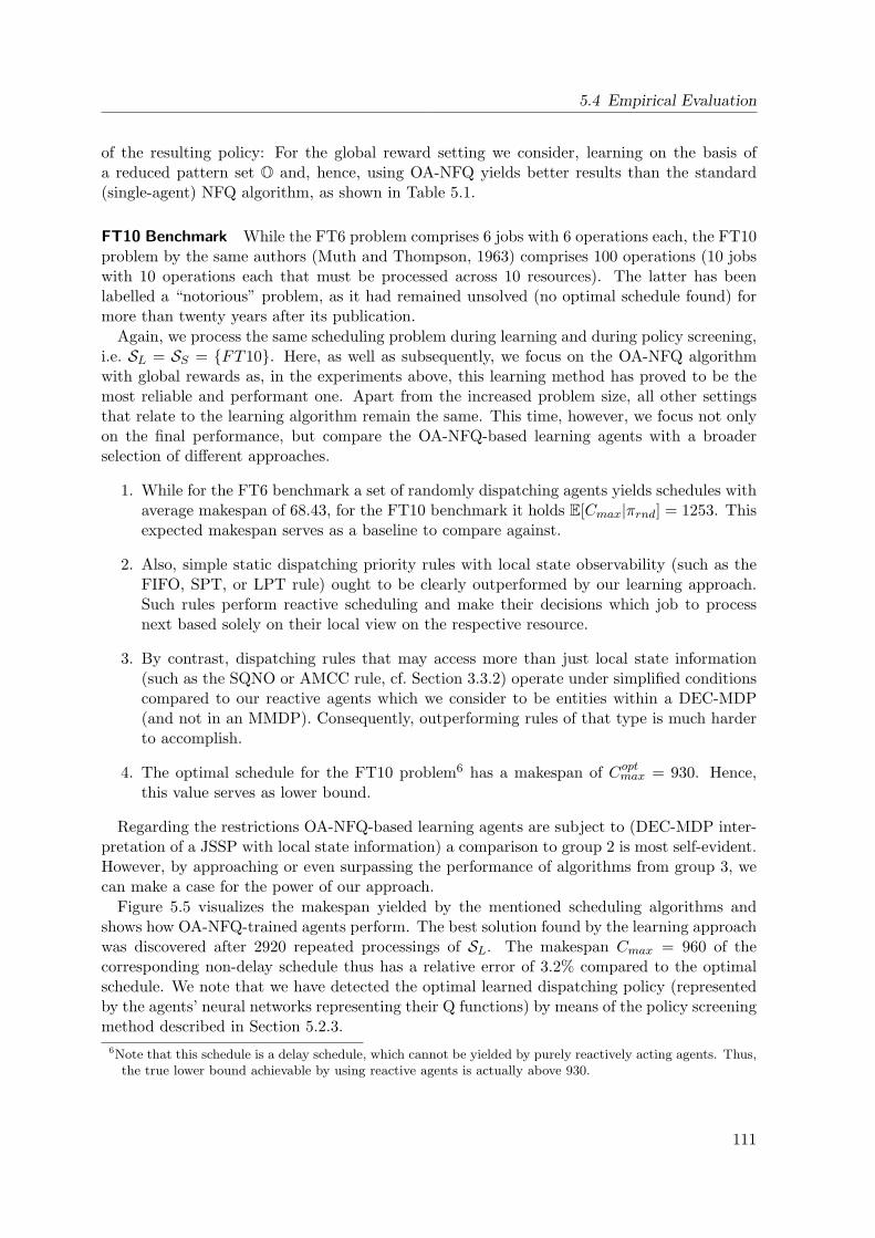
5.4 Empirical Evaluation
of the resulting policy: For the global reward setting we consider, learning on the basis ofa reduced pattern set O and, hence, using OA-NFQ yields better results than the standard(single-agent) NFQ algorithm, as shown in Table 5.1.
FT10 Benchmark While the FT6 problem comprises 6 jobs with 6 operations each, the FT10problem by the same authors (Muth and Thompson, 1963) comprises 100 operations (10 jobswith 10 operations each that must be processed across 10 resources). The latter has beenlabelled a “notorious” problem, as it had remained unsolved (no optimal schedule found) formore than twenty years after its publication.
Again, we process the same scheduling problem during learning and during policy screening,i.e. SL = SS = FT10. Here, as well as subsequently, we focus on the OA-NFQ algorithmwith global rewards as, in the experiments above, this learning method has proved to be themost reliable and performant one. Apart from the increased problem size, all other settingsthat relate to the learning algorithm remain the same. This time, however, we focus not onlyon the final performance, but compare the OA-NFQ-based learning agents with a broaderselection of different approaches.
1. While for the FT6 benchmark a set of randomly dispatching agents yields schedules withaverage makespan of 68.43, for the FT10 benchmark it holds E[Cmax|πrnd] = 1253. Thisexpected makespan serves as a baseline to compare against.
2. Also, simple static dispatching priority rules with local state observability (such as theFIFO, SPT, or LPT rule) ought to be clearly outperformed by our learning approach.Such rules perform reactive scheduling and make their decisions which job to processnext based solely on their local view on the respective resource.
3. By contrast, dispatching rules that may access more than just local state information(such as the SQNO or AMCC rule, cf. Section 3.3.2) operate under simplified conditionscompared to our reactive agents which we consider to be entities within a DEC-MDP(and not in an MMDP). Consequently, outperforming rules of that type is much harderto accomplish.
4. The optimal schedule for the FT10 problem6 has a makespan of Coptmax = 930. Hence,this value serves as lower bound.
Regarding the restrictions OA-NFQ-based learning agents are subject to (DEC-MDP inter-pretation of a JSSP with local state information) a comparison to group 2 is most self-evident.However, by approaching or even surpassing the performance of algorithms from group 3, wecan make a case for the power of our approach.
Figure 5.5 visualizes the makespan yielded by the mentioned scheduling algorithms andshows how OA-NFQ-trained agents perform. The best solution found by the learning approachwas discovered after 2920 repeated processings of SL. The makespan Cmax = 960 of thecorresponding non-delay schedule thus has a relative error of 3.2% compared to the optimalschedule. We note that we have detected the optimal learned dispatching policy (representedby the agents’ neural networks representing their Q functions) by means of the policy screeningmethod described in Section 5.2.3.
6Note that this schedule is a delay schedule, which cannot be yielded by purely reactively acting agents. Thus,the true lower bound achievable by using reactive agents is actually above 930.
111
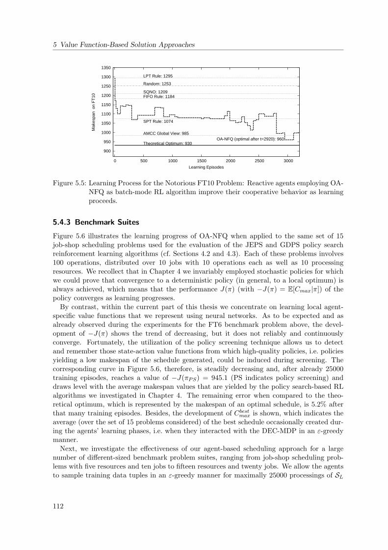
5 Value Function-Based Solution Approaches
900
950
1000
1050
1100
1150
1200
1250
1300
1350
0 500 1000 1500 2000 2500 3000
Mak
espa
n o
n F
T10
Learning Episodes
LPT Rule: 1295
Random: 1253
FIFO Rule: 1184
SPT Rule: 1074
OA-NFQ (optimal after t=2920): 960Theoretical Optimum: 930
AMCC Global View: 985
SQNO: 1209
Figure 5.5: Learning Process for the Notorious FT10 Problem: Reactive agents employing OA-NFQ as batch-mode RL algorithm improve their cooperative behavior as learningproceeds.
5.4.3 Benchmark Suites
Figure 5.6 illustrates the learning progress of OA-NFQ when applied to the same set of 15job-shop scheduling problems used for the evaluation of the JEPS and GDPS policy searchreinforcement learning algorithms (cf. Sections 4.2 and 4.3). Each of these problems involves100 operations, distributed over 10 jobs with 10 operations each as well as 10 processingresources. We recollect that in Chapter 4 we invariably employed stochastic policies for whichwe could prove that convergence to a deterministic policy (in general, to a local optimum) isalways achieved, which means that the performance J(π) (with −J(π) = E[Cmax|π]) of thepolicy converges as learning progresses.
By contrast, within the current part of this thesis we concentrate on learning local agent-specific value functions that we represent using neural networks. As to be expected and asalready observed during the experiments for the FT6 benchmark problem above, the devel-opment of −J(π) shows the trend of decreasing, but it does not reliably and continuouslyconverge. Fortunately, the utilization of the policy screening technique allows us to detectand remember those state-action value functions from which high-quality policies, i.e. policiesyielding a low makespan of the schedule generated, could be induced during screening. Thecorresponding curve in Figure 5.6, therefore, is steadily decreasing and, after already 25000training episodes, reaches a value of −J(πPS) = 945.1 (PS indicates policy screening) anddraws level with the average makespan values that are yielded by the policy search-based RLalgorithms we investigated in Chapter 4. The remaining error when compared to the theo-retical optimum, which is represented by the makespan of an optimal schedule, is 5.2% afterthat many training episodes. Besides, the development of Cbestmax is shown, which indicates theaverage (over the set of 15 problems considered) of the best schedule occasionally created dur-ing the agents’ learning phases, i.e. when they interacted with the DEC-MDP in an ε-greedymanner.
Next, we investigate the effectiveness of our agent-based scheduling approach for a largenumber of different-sized benchmark problem suites, ranging from job-shop scheduling prob-lems with five resources and ten jobs to fifteen resources and twenty jobs. We allow the agentsto sample training data tuples in an ε-greedy manner for maximally 25000 processings of SL
112
5.4 Empirical Evaluation
Figure 5.6: Learning Progress of OA-NFQ for a Set of 10x10 JSSPs: The solid line indicates theperformance of those top policies that were detected by means of policy screening.All curves are averaged over the 15 problems considered.
with SL = SS and permitted intermediate calls to OA-NFQ (again, N = 20 iterations of theQ iteration loop) in order to reach the vicinity of a near-optimal Q function as quickly aspossible. Here, all resulting value functions and corresponding greedy multi-agent policies areevaluated (tested during the application phase) on the same problems as used during learning(SL = SA).
For a better illustration of the findings we have grouped the results on individual benchmarkproblems into classes with respect to the numbers of resources and jobs to be processed (Figure5.7). As before, all benchmark problems are taken from the Operations Research Library7
(Beasley, 2005). Although these benchmarks are of different sizes, they have in common thatno recirculation occurs and that each job has to be processed on each resource exactly once.The results are given relative to the makespan of the optimal schedule (100%, black data series).Data series colored in light gray correspond to static rules having local state information only(group 2 from the above enumeration of algorithms to compare against), whereas medium gray-colored ones are not subject to that restriction (group 3). The dark gray-colored data seriescorresponds to our approach using independent batch-mode reinforcement learning agents thatdetermine their value functions using OA-NFQ which is based on the DEC-MDP interpretationof JSSPs and, hence, is restricted to the local view, too.
For the 5 × 15 (LA6-10) and 5 × 20 (LA11-15) benchmark problems, the optimal solutioncan be found by our learning approach in all cases. This depicts an impressive result as itmeans that the optimal schedule in terms of minimal makespan is created for each of theseproblem instances, if each of the agents exploits its acquired local value function Qi greedily.
For the 5 × 10 (LA1-5) and 10 × 10 (LA16-20, ORB1-9) sets, only a small relative errorof less than ten percent compared to the optimal makespan remains (3.4/4.0/7.2%). As tobe expected, dispatching rules, even those disposing of more than just local state information(AMCC, SQNO), are clearly outperformed. For the larger benchmarks (ABZ) involving 15resources and 20 jobs per problem instance the relative error increases to 10.6%, but therule-based schedulers can be outperformed still.
7Benchmark problems ABZ5-9 were originally generated by Adams et al. (1988), problems ORB01-09 byApplegate and Cook (1991), and finally, problems LA1-20 are due to Lawrence (1984).
113
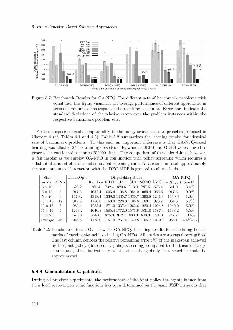
5 Value Function-Based Solution Approaches
100
105
110
115
120
125
130
135
140
5x10 (LA1-5) 5x15 (LA6-10) 5x20 (LA11-15) 10x10 (LA16-20) 10x10 (ORB1-9) 15x20 (ABZ7-9)
Ave
rage
Mak
espa
n R
elat
ive
To
Opt
imal
Mak
espa
n (%
)
Name of Benchmark Set and Problem Size (#resources x #jobs)
103.35
100.00 100.00
104.02107.17
110.58
FIFO RuleLPT RuleSPT Rule
SQNO RuleAMCC Rule
OA-NFQTheor. Optimum
Figure 5.7: Benchmark Results for OA-NFQ: For different sets of benchmark problems withequal size, this figure visualizes the average performance of different approaches interms of minimized makespan of the resulting schedules. Error bars indicate thestandard deviations of the relative errors over the problem instances within therespective benchmark problem sets.
For the purpose of result comparability to the policy search-based approaches proposed inChapter 4 (cf. Tables 4.1 and 4.2), Table 5.2 summarizes the learning results for identicalsets of benchmark problems. To this end, an important difference is that OA-NFQ-basedlearning was allotted 25000 training episodes only, whereas JEPS and GDPS were allowed toprocess the considered scenarios 250000 times. The comparison of these algorithms, however,is fair insofar as we employ OA-NFQ in conjunction with policy screening which requires asubstantial amount of additional simulated screening runs. As a result, in total approximatelythe same amount of interaction with the DEC-MDP is granted to all methods.
Size Theor.Opt. Dispatching Rules OA-NFQm× n #Prbl Random FIFO LPT SPT SQNO AMCC −J(πPS) Rem.Err.5× 10 5 620.2 765.4 732.4 829.6 713.0 787.6 673.4 641.0 3.4%5× 15 5 917.6 1052.4 1003.6 1108.8 1054.0 1065.4 955.6 917.6 0.0%5× 20 6 1179.2 1358.4 1339.0 1435.7 1330.7 1390.8 1241.8 1190.8 1.0%10× 10 17 912.5 1158.0 1153.0 1228.3 1106.3 1163.1 973.7 964.3 5.7%10× 15 5 983.4 1285.3 1271.0 1337.4 1263.6 1220.4 1094.8 1042.2 6.0%15× 15 5 1263.2 1640.8 1585.4 1772.0 1573.6 1531.0 1387.4 1333.2 5.5%15× 20 3 676.0 878.0 875.3 942.7 888.3 843.3 771.0 747.7 10.6%Average 46 946.5 1178.0 1157.0 1251.4 1140.8 1166.7 1019.0 988.1 4.4%±3.5
Table 5.2: Benchmark Result Overview for OA-NFQ: Learning results for scheduling bench-marks of varying size achieved using OA-NFQ. All entries are averaged over #Prbl.The last column denotes the relative remaining error (%) of the makespan achievedby the joint policy (detected by policy screening) compared to the theoretical op-timum and, thus, indicates to what extent the globally best schedule could beapproximated.
5.4.4 Generalization Capabilities
During all previous experiments, the performance of the joint policy the agents induce fromtheir local state-action value functions has been determined on the same JSSP instances that
114
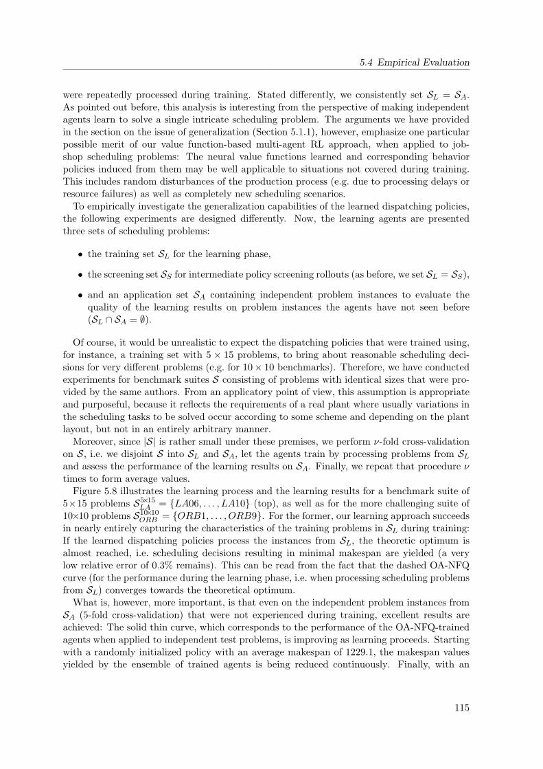
5.4 Empirical Evaluation
were repeatedly processed during training. Stated differently, we consistently set SL = SA.As pointed out before, this analysis is interesting from the perspective of making independentagents learn to solve a single intricate scheduling problem. The arguments we have providedin the section on the issue of generalization (Section 5.1.1), however, emphasize one particularpossible merit of our value function-based multi-agent RL approach, when applied to job-shop scheduling problems: The neural value functions learned and corresponding behaviorpolicies induced from them may be well applicable to situations not covered during training.This includes random disturbances of the production process (e.g. due to processing delays orresource failures) as well as completely new scheduling scenarios.
To empirically investigate the generalization capabilities of the learned dispatching policies,the following experiments are designed differently. Now, the learning agents are presentedthree sets of scheduling problems:
• the training set SL for the learning phase,
• the screening set SS for intermediate policy screening rollouts (as before, we set SL = SS),
• and an application set SA containing independent problem instances to evaluate thequality of the learning results on problem instances the agents have not seen before(SL ∩ SA = ∅).
Of course, it would be unrealistic to expect the dispatching policies that were trained using,for instance, a training set with 5 × 15 problems, to bring about reasonable scheduling deci-sions for very different problems (e.g. for 10× 10 benchmarks). Therefore, we have conductedexperiments for benchmark suites S consisting of problems with identical sizes that were pro-vided by the same authors. From an applicatory point of view, this assumption is appropriateand purposeful, because it reflects the requirements of a real plant where usually variations inthe scheduling tasks to be solved occur according to some scheme and depending on the plantlayout, but not in an entirely arbitrary manner.
Moreover, since |S| is rather small under these premises, we perform ν-fold cross-validationon S, i.e. we disjoint S into SL and SA, let the agents train by processing problems from SLand assess the performance of the learning results on SA. Finally, we repeat that procedure νtimes to form average values.
Figure 5.8 illustrates the learning process and the learning results for a benchmark suite of5×15 problems S5×15
LA = LA06, . . . , LA10 (top), as well as for the more challenging suite of10×10 problems S10×10
ORB = ORB1, . . . , ORB9. For the former, our learning approach succeedsin nearly entirely capturing the characteristics of the training problems in SL during training:If the learned dispatching policies process the instances from SL, the theoretic optimum isalmost reached, i.e. scheduling decisions resulting in minimal makespan are yielded (a verylow relative error of 0.3% remains). This can be read from the fact that the dashed OA-NFQcurve (for the performance during the learning phase, i.e. when processing scheduling problemsfrom SL) converges towards the theoretical optimum.
What is, however, more important, is that even on the independent problem instances fromSA (5-fold cross-validation) that were not experienced during training, excellent results areachieved: The solid thin curve, which corresponds to the performance of the OA-NFQ-trainedagents when applied to independent test problems, is improving as learning proceeds. Startingwith a randomly initialized policy with an average makespan of 1229.1, the makespan valuesyielded by the ensemble of trained agents is being reduced continuously. Finally, with an
115
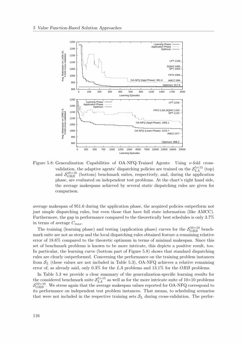
5 Value Function-Based Solution Approaches
900
950
1000
1050
1100
1150
1200
1250
20001700140011008005004003002001000
Avg
. Mak
espa
n on
LA
06-1
0,
5-f
old
cros
s-va
lidat
ed
Learning Episodes
OA-NFQ (Appl.Phase): 951.6
Optimum: 917.6
FIFO:1004
LPT:1109
SPT:1054SQNO:1065
AMCC:956
Learning PhaseApplication Phase
Optimum
900
950
1000
1050
1100
1150
1200
1250
20000165001350010500750045001500125010007505002500
Avg
. Mak
espa
n on
OR
B1-
9,
3-f
old
cros
s-va
lidat
ed
Learning Episodes
OA-NFQ (Appl.Phase): 1065.1
OA-NFQ (Learn.Phase): 1015.7
Optimum: 898.2
FIFO:1164,SQNO:1163
LPT:1226
SPT:1142
AMCC:977
Learning PhaseApplication Phase
Optimum
Figure 5.8: Generalization Capabilities of OA-NFQ-Trained Agents: Using ν-fold cross-validation, the adaptive agents’ dispatching policies are trained on the S5×15
LA (top)and S10×10
ORB (bottom) benchmark suites, respectively, and, during the applicationphase, are evaluated on independent test problems. At the chart’s right hand side,the average makespans achieved by several static dispatching rules are given forcomparison.
average makespan of 951.6 during the application phase, the acquired policies outperform notjust simple dispatching rules, but even those that have full state information (like AMCC).Furthermore, the gap in performance compared to the theoretically best schedules is only 3.7%in terms of average Cmax.
The training (learning phase) and testing (application phase) curves for the S10×10ORB bench-
mark suite are not as steep and the local dispatching rules obtained feature a remaining relativeerror of 18.6% compared to the theoretic optimum in terms of minimal makespan. Since thisset of benchmark problems is known to be more intricate, this depicts a positive result, too.In particular, the learning curve (bottom part of Figure 5.8) shows that standard dispatchingrules are clearly outperformed. Concerning the performance on the training problem instancesfrom SL (these values are not included in Table 5.3), OA-NFQ achieves a relative remainingerror of, as already said, only 0.3% for the LA problems and 13.1% for the ORB problems.
In Table 5.3 we provide a clear summary of the generalization-specific learning results forthe considered benchmark suite S5×15
LA as well as for the more intricate suite of 10×10 problemsS10×10ORB . We stress again that the average makespan values reported for OA-NFQ correspond to
its performance on independent test problem instances. That means, to scheduling scenariosthat were not included in the respective training sets SL during cross-validation. The perfor-
116
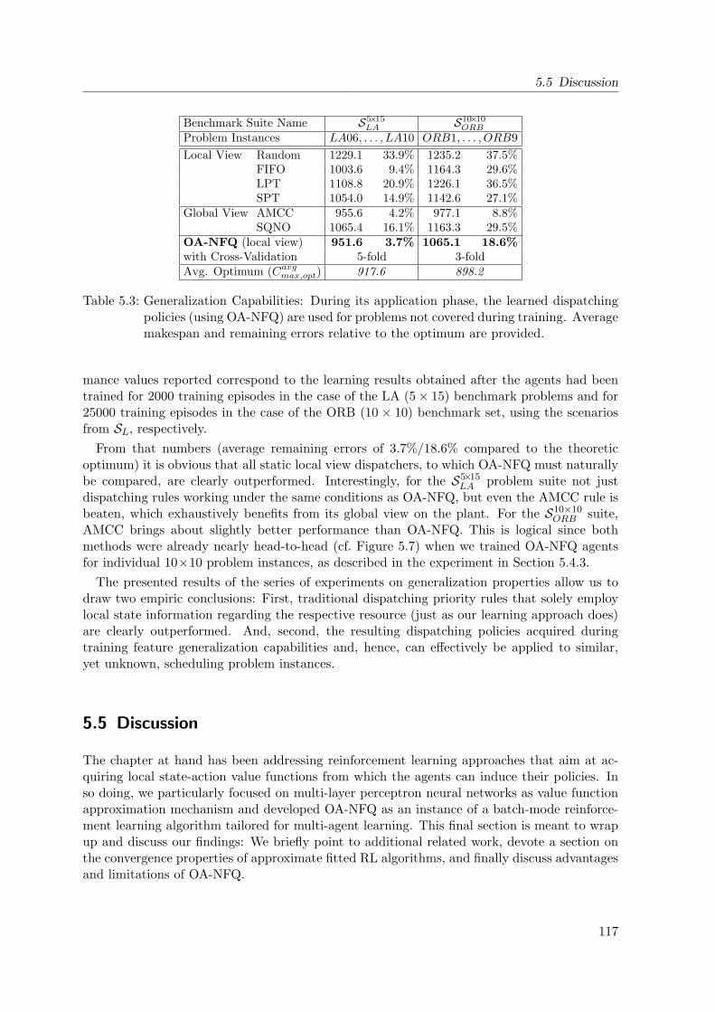
5.5 Discussion
Benchmark Suite Name S5×15LA S10×10
ORB
Problem Instances LA06, . . . , LA10 ORB1, . . . , ORB9Local View Random 1229.1 33.9% 1235.2 37.5%
FIFO 1003.6 9.4% 1164.3 29.6%LPT 1108.8 20.9% 1226.1 36.5%SPT 1054.0 14.9% 1142.6 27.1%
Global View AMCC 955.6 4.2% 977.1 8.8%SQNO 1065.4 16.1% 1163.3 29.5%
OA-NFQ (local view) 951.6 3.7% 1065.1 18.6%with Cross-Validation 5-fold 3-foldAvg. Optimum (Cavg
max,opt) 917.6 898.2
Table 5.3: Generalization Capabilities: During its application phase, the learned dispatchingpolicies (using OA-NFQ) are used for problems not covered during training. Averagemakespan and remaining errors relative to the optimum are provided.
mance values reported correspond to the learning results obtained after the agents had beentrained for 2000 training episodes in the case of the LA (5× 15) benchmark problems and for25000 training episodes in the case of the ORB (10 × 10) benchmark set, using the scenariosfrom SL, respectively.
From that numbers (average remaining errors of 3.7%/18.6% compared to the theoreticoptimum) it is obvious that all static local view dispatchers, to which OA-NFQ must naturallybe compared, are clearly outperformed. Interestingly, for the S5×15
LA problem suite not justdispatching rules working under the same conditions as OA-NFQ, but even the AMCC rule isbeaten, which exhaustively benefits from its global view on the plant. For the S10×10
ORB suite,AMCC brings about slightly better performance than OA-NFQ. This is logical since bothmethods were already nearly head-to-head (cf. Figure 5.7) when we trained OA-NFQ agentsfor individual 10×10 problem instances, as described in the experiment in Section 5.4.3.
The presented results of the series of experiments on generalization properties allow us todraw two empiric conclusions: First, traditional dispatching priority rules that solely employlocal state information regarding the respective resource (just as our learning approach does)are clearly outperformed. And, second, the resulting dispatching policies acquired duringtraining feature generalization capabilities and, hence, can effectively be applied to similar,yet unknown, scheduling problem instances.
5.5 Discussion
The chapter at hand has been addressing reinforcement learning approaches that aim at ac-quiring local state-action value functions from which the agents can induce their policies. Inso doing, we particularly focused on multi-layer perceptron neural networks as value functionapproximation mechanism and developed OA-NFQ as an instance of a batch-mode reinforce-ment learning algorithm tailored for multi-agent learning. This final section is meant to wrapup and discuss our findings: We briefly point to additional related work, devote a section onthe convergence properties of approximate fitted RL algorithms, and finally discuss advantagesand limitations of OA-NFQ.
117
5 Value Function-Based Solution Approaches
5.5.1 Related Work
Optimistic assumption-based neural fitted Q iteration (OA-NFQ) is a neural value function-based batch-mode RL algorithm that we developed with the intention of making independentlyacting and learning agents acquire approximately optimal policies within cooperative multi-agent settings. On the one hand, being an instance of the fitted Q iteration family of RLalgorithms, OA-NFQ is of course related to the work by Ernst et al. (2006) on FQI and, evenmore, to the NFQ algorithm of which it is a direct extension (cf. Section 5.2.2, Riedmiller,2005). On the other hand, Q learning based on the optimistic assumption is due to the workby Lauer and Riedmiller (2000). Our optimistic batch-mode learning approach is thus relatedto that piece of work as well, though extended for decentralized MDP settings with partialstate observability.
Moreover, the idea of using distributed, agent-specific value functions, i.e. local value func-tions belonging to the agents, originates from the work by Schneider et al. (1999). Thisapproach has thenceforth been applied in the context of different applications, for examplefor energy distribution networks (Schneider et al., 1998) or for mobile robot planning andintelligent traffic systems (Ferreira and Khosla, 2000).
The issue of local versus global rewards within cooperative multi-agent systems, which wehave touched only briefly, is in the center of the research by Agogino and Tumer (2005) andTumer and Agogino (2004). Their focus is on the design of agent-specific utility functions (costor reward functions) that are factored in that there is a strong correlation between individualagent rewards and the performance of the team as a whole, and that are highly learnableby each single agent, meaning that any agent’s contribution to the success of the team isconsidered appropriately.
While the exact relations to other researchers’ work mentioned afore have been discussedthoroughly in the preceding sections of this chapter, we shall focus on the convergence prop-erties of our approach and corresponding related work, next. Besides, regarding related ap-proaches to solving job-shop scheduling problems using value function-based reinforcementlearning we refer to the section on related work in Chapter 3 (Section 3.3). And, for anoverview of further model-free RL approaches for learning in cooperative multi-agent systemswe point to Section 2.5.
Convergence Issues and Problems
The fitted Q iteration learning scheme outlined in Section 5.1.2 tries to iteratively minimizethe Bellman error (cf. Equation 5.3) over the set T of experience tuples. The supervisedlearning component involved, i.e. the function approximator fitting part, however, makes usraise the question to which extent does Bellman error minimization imply convergence to a(near-)optimal policy when used in conjunction with function approximation?
In general, for several algorithms, it is expected that convergence cannot be achieved and aphenomenon called “chattering” occurs. The space Q of all Q functions can be divided intoregions where a constant policy (given by greedy Q exploitation) is followed. Bertsekas andTsitsiklis (1996) call these regions greedy regions because each one corresponds to a differentgreedy policy and has its own greedy point – the point in Q to which Q(·) moves in the courseof learning. If it happens that the greedy point does not lie in its greedy region, the policylearned will fluctuate between two or more greedy policies that share the same boundary inQ. More details and a deeper analysis of the chattering problem can be found in the paper by
118

5.5 Discussion
Gordon (1996) and the book by Bertsekas and Tsitsiklis (1996).As a matter of fact, much of the literature has focused on gaining insights into the conver-
gence behavior of approximate RL, e.g. on the soundness of approximate value iteration orpolicy iteration (Munos, 2005, 2003). Nevertheless, there are also various publications report-ing on negative results using reinforcement learning approaches with function approximation,many of which head into a specific direction: The policy the learning agent acquires quicklyreaches a remarkable quality, but in the further course of learning a significant policy degra-dation can be observed. So, for instance, Bertsekas and Tsitsiklis (1996) report on attemptsto learn a policy for playing the game of Tetris and point out the paradoxical observation thathigh performance is achieved after relatively few policy iterations, but then the performancedrops. Gaskett (2002) has trained a Q controller for the cart pole benchmark and obtainedexcellent results initially. But, despite trying several approaches in an attempt to reduce policydegradation, these results got lost in the further course of learning. Weaver and Baxter (1999)performed experiments with a backgammon-playing learning agent and observed reduced play-ing performance while improving the accuracy of value function approximation concurrently.Bertsekas et al. (2000) made similar observations, when applying a neuro-dynamic program-ming approach to a missile defense problem: The sequence of policies generated during learningdid not converge; improvements could be obtained in the initial iterations and once the vicinityof the optimal value function had been reached, oscillations occurred. Munos (2003) dividesthe learning process into a transitional and a stationary phase. During the former, rapidimprovements in policy quality can be made due to a comparatively good value function ap-proximation, when compared to the closeness to the optimality (|Qq−TQq−1| is low comparedto |TQq−1 − Q?|)8. Therefore, he argues that a greedy policy with respect to Qq is likely tobe superior to the policy represented by greedy exploitation of TQq−1.
Regarding the goal to obtain a more stable learning progress and near-optimal policies thereare several related publications. Kakade and Langford (2002) point out to the fact that approx-imate value function methods suffer from insufficient theoretical results on the performance ofa policy based on approximated values. Working with stochastic policies and within an onlinepolicy iteration setting, they propose a conservative policy iteration method which seeks to find“approximately” optimal solutions by stopping to iterate when the estimated policy advantagefrom one iteration to the next drops below some threshold. Boyan and Moore (1995) stressthat dynamic programming approaches in combination with function approximation can bringabout wrong policies even in very benign cases. They suggest an algorithm, called GrowSup-port, that uses simulations with the current greedy policy (roll-outs) to determine state valuesand successively adds elements to a set of state values whose final value has been determined.Weaver and Baxter (1999) have introduced an extended version of TD(λ) that is based onstate-value differences and demonstrated its successful applicability for a toy problem and forthe acrobot benchmark.
As pointed out in Section 5.2.3, neural networks belong to the class of “exaggerating” valuefunction approximation mechanisms (Gordon, 1996) and as such feature the potential riskof diverging. This problem concerns NFQ as well and, accordingly, a number of extensionshave been proposed that aim at stabilizing this algorithm’s learning performance. For exam-ple, monitored Q iteration has been suggested as an approach to circumvent effects of policydegradation during advanced stages of learning (Gabel and Riedmiller, 2006b). Here, the basicidea is to define an alternative error measure which more directly relates to a policy’s actual
8The operator T is the Bellman operator which was introduced in Section 2.1.5.
119
5 Value Function-Based Solution Approaches
performance, to create the conditions that this error measure can be effectively calculated dur-ing learning, and to continuously monitor the learning process utilizing the alternative errormeasure. In so doing, top-performing policies are remembered and also an early stopping oflearning is facilitated.
As stressed before, in the context of this thesis we mostly relied on the – admittedly time-consuming, but simple and effective – policy screening technique (Section 5.2.3) in order toevaluate the trained policies. Improving this technique is also the topic of current research. Forexample, Kietzmann and Riedmiller (2009) argue that it is possible to select the most promisingpolicies out of the set of all intermediately created policies and to do the screening only forthat subset. The resulting method, offline policy evaluation, helps in avoiding an extensivesimulated evaluation of all generated policies and, thus, saves computational resources, whileit still allows for figuring out a nearly optimal policy.
5.5.2 Advantages and Limitations of OA-NFQ
The learning of optimal value functions with the succeeding derivation of a policy representsthe predominant approach to tackle reinforcement learning problems. In this chapter, we haveexplored batch-mode RL approaches and, specifically, suggested a novel multi-agent batch RLalgorithm, OA-NFQ.
The approach we have taken has proved to be very powerful when employed for learningjoint dispatching policies for job-shop scheduling problems modelled as decentralized Markovdecision processes. When compared to the default approach to solving JSSPs in a centralizedmanner, we benefit from the idea of “distribute and conquer”. The trained agents can quickly,independently, and with minimal computational effort decide for their action (calculatingQi(si, α∀α ∈ A(si) suffices, i.e. basically |si| forward sweeps through the neural net thatrepresents Qi are necessary).
Of course, in this manner the optimal joint action will not always be executed, but ourexperimental studies confirm that the decisions made by the agents are of high quality, yieldingnear-optimal schedules in terms of minimizing makespan after all. Equally important, thecorresponding policies learned are acquired after little training time, i.e. after little interactionwith the simulated scheduling plant. This can be mainly tributed to the data-efficient natureof batch-mode reinforcement learning algorithms.
The probably most convincing and outstanding characteristic of our value function-basedapproach to finding near-optimal joint policies for DEC-MDPs is that the OA-NFQ algorithmfeatures excellent generalization capabilities. Of course, during the training phase it entails therequirement of learning in a deterministic environment, but after the agents have acquired theirlocal policies, they may apply them for stochastic and, more importantly, completely differentscheduling problems. In so doing, standard approaches that perform reactive scheduling withlocal observations (like dispatching priority rules) can be outperformed clearly.
While the RL approaches based on policy search examined in Chapter 4 exhibit a ratherstrong dependency on several learning parameters, we stress that the combination of methodsinvolved in the development of the OA-NFQ algorithm, resulted in a very low parametersensitivity. Relatively straightforward design decisions with respect to parameters as well asstate and action features already brought about convincing learning results and varying themhad only a minor impact on learning performance. To this end, for instance, investing morefeature engineering effort might even further increase the capabilities of OA-NFQ.
Value function-based reinforcement learning is also afflicted with certain limitations. Pol-
120
5.5 Discussion
icy search RL approaches are capable of significantly restricting the space of policies to beconsidered during learning (given that adequate task knowledge is available). By contrast,value function-based RL more strongly suffers from the “curse of dimensionality”, i.e. fromthe exponential increase of the state space as the problem dimension grows. In principle, theyhave to take into account each state-action pair separately and, hence, would consume anexponential amount of memory to store the value function. We have tackled this issue in twodifferent ways: First, we have restricted ourselves to factored state representations, where theglobal state can be broken up into m smaller local ones. Second, we avoided a table-basedexact representation of the value function and instead employed multi-layer perceptrons asa value function approximation scheme that is known to be powerful and to feature goodgeneralization capabilities.
Applying value function approximation, however, generally comes with the cost that con-vergence guarantees of various RL algorithms no longer hold. Furthermore, the use of neuralnetworks for that task brings the risk of “exaggerating” certain state-action value estimates(Section 5.4.2). To this end, we relied on the policy screening technique in order to select thebest-performing policies generated during learning.
Having spoken about possibly enormous memory requirements for value function-based RL,this issue also concerns the batch-mode learning part of our approach. Working with growingtransition tuple sets, of course, the training times when fitting a function approximator for thepattern set generated increases. At this, our interpretation and integration of the optimisticassumption into OA-NFQ has yielded some relief. Thus, the OA part of this algorithm servestwo purposes: It enables improved (optimistic) inter-agent coordination and at the same timereduces learning times as only a fraction of the data collected is actually exploited when doingfitted Q iteration.
Our approach to model the scheduling task as a sequential decision problem and to makereactive scheduling decisions features the disadvantage that, in the form presented, the result-ing schedules correspond to solutions from the set of non-delay schedules, only: If a resourcehas finished processing one operation and has at least one job waiting, the dispatching agentimmediately continues processing by picking one of the waiting jobs. Our approach does notallow a resource to remain idle, if there is more work to be done.
From scheduling theory, however, it is well-known that for certain scheduling problem in-stances the optimal schedule may very well be a delay schedule (cf. Section 3.1.1). As visu-alized in Figure 3.2 on page 33, the following subset inclusion holds for three sub-classes ofnon-preemptive schedules
Snondelay ( Sactive ( Ssemiactive ( S
where S denotes the set of all possible schedules (Pinedo, 2002). The optimal schedule for aparticular problem, however, is always within Sactive, but not necessarily within Snondelay. Asa consequence, our approach will fail to find the optimal solution for many problem instances,but is capable of generating near-optimal schedules from Snondelay. For these reasons, one ofour main goals to be pursued in the next chapter is to extend our learning framework to allowfor the generation of delay schedules. In so doing, we are going to refrain from making theagents behave purely reactively (as we did up to here) and, moreover, we will allow them toemploy a limited form of communication in order to resolve certain inter-agent dependencies.
121

5 Value Function-Based Solution Approaches
122
6 Communicating Agents and OptimalSchedules
In the previous two chapters, we were concerned with approximate solution approaches forDEC-MDPs with changing action sets that basically relied on reactively acting and learningindependent agents. We have emphasized that this kind of reactivity does not always allow forfinding optimal policies because the learners are memoryless and unable to take inter-agentdependencies into account properly. By contrast, the notion of jointly optimal team behaviorwill shift into our focus in the chapter at hand.
In particular, we will investigate two orthogonal approaches that enable the learners toexecute optimal local policies – based on state history information as well as on communication– and we will integrate these concepts with (some of) the reinforcement learning methods wedeveloped in Chapter 4 and 5.
We start by providing some foundations on reactive policies and their limitations as wellas on the relevance of an agent’s interaction history. In Section 6.2, we describe the twomentioned approaches that are meant to enhance the learning agents’ capabilities in yieldingoptimal joint policies. Subsequently, we evaluate certain combinations of these approacheswith the distributed reinforcement learning algorithms proposed in earlier chapters for variousjob-shop scheduling problems. And, finally, in Section 6.4 we conclude with a discussion ofour findings and related work.
6.1 Foundations
The agents we are considering do not possess a model of the environment, but have to learngood behavior by repeatedly interacting with their environment. As we have seen, the learningtask within decentralized Markov decision processes is aggravated, when compared to learningwithin single-agent MDPs, mainly by two complicating factors: the inability of each agent tofully observe the global system state as well as the presence of multiple, independently actingagents.
Moreover, a third factor that complicates the finding of jointly optimal policies must beattributed to us: Within the scope of the policy search-based and value function-based re-inforcement learning methods that we developed in Chapter 4 and 5, we always made thelearning agents employ reactive local policies. This kind of memorylessness, of course, im-pedes the task of learning good behavior within an environment that each agent perceives asnon-Markovian due to the former two reasons mentioned.
6.1.1 Reactive Policies and Their Limitations
An agent taking its action based solely on its most recent local observation si ⊆ Ai will ingeneral not be able to contribute to optimal corporate behavior. In particular, it will havedifficulties in assessing the value of taking its idle action α0. Taking α0, the local state remains
123
6 Communicating Agents and Optimal Schedules
unchanged except when it is influenced by dependent actions of other agents. Since a purelyreactive agent, however, has no information related to other agents and dependencies at all, itis incapable of properly distinguishing when it is favorable to remain idle and when not. Forthese reasons, we have excluded α0 from all Ai for purely reactive agents.
Definition 6.1 (Reactive Policy).For a factored m-agent DEC-MDP with changing action sets and partially ordered transitiondependencies, a reactive policy πr = 〈πr1 . . . πrm〉 consists of m reactive local policies withπri : Si → Ari where Si = P(Ari ).
That is, purely reactive policies always take an action α ∈ Ai(si) = si (except for si = ∅),even if it was more advisable to stay idle and wait for a transition from si to some s′i = si∪α′induced by another agent, and then execute α′ in s′i.
6.1.2 Interaction Histories
Oliehoek et al. (2008a) have shown that there exists at least one optimal deterministic jointpolicy for each DEC-POMDP. Thus, although the utilization of stochastic policies can bebeneficial during learning, it is basically sufficient to restrict attention to deterministic policieswhile still allowing for jointly optimal behavior.
For decentralized MDPs with changing action sets and partially ordered transition depen-dencies there are, after D decision stages, at maximum (2|A
ri |)D possible local state histories
for agent i. As a consequence, there are a total of
D−1∑d=0
(2|Ari |)d =
(2|Ari |)D − 1
2|Ari | − 1
such sequences for agent i. However, when taking into account the execute-once property ofthe class of DEC-MDPs we are addressing (cf. Lemma 1), we obtain a total number of
|Ari |−1∑d=0
(|Ari | − d)(2|Ari |)d
of possible local policies for agent i, which is doubly exponential in the number of decisionstages and, hence, in the number of available actions for that agent.
When not using reactive agents, but those that base their action choices on the full interac-tion history, we enable the team as a whole to acquire optimal behavior. Unfortunately, thelocal policies must then be defined over sequences of local states si ∈ Si which brings aboutan exponential blow-up in the size of the domain over which πi is defined. Needless to say thatsuch an approach quickly renders infeasible as the problem size considered grows. Having inmind that we intend to work with rather intricate and larger-scaled scheduling problems, werefrain from pursuing this straightforward approach. Instead, in what follows we
• seize the idea of using a highly compact representation of an agent’s interaction historywhich we developed in Section 2.4.3. In so doing, we exploit properties of DEC-MDPswith changing action sets in a purposeful manner. While this approach still forces us tohandle a clearly increased state space, we do not have to face the exponential increasejust mentioned.
124
6.2 Resolving Transition Dependencies
• As a second, orthogonal approach, we intend to resolve some of the state transitiondependencies between agents. From an agent’s point of view, this yields an at least partialreconstitution of the Markov property as the effect of the inter-agent dependencies – asmodelled by means of dependency functions σi (cf. Definition 2.13) – are made explicit.Moreover, the agents’ policies remain reactive ones which keeps the state space to beconsidered at a moderate size.
From an applicatory perspective, both approaches are intended as a mean to create optimalpolicies. In terms of job-shop scheduling tasks, this specifically addresses the capability tocreate delay schedules. As a reminder, delay schedules arise, if at some point of processingat least one resource remains idle although currently at least one job is waiting for furtherprocessing at the resource considered. By contrast, a reactive dispatching agent would pickone of the waiting jobs, immediately continue its processing, and in so doing, yield a non-delay schedule. As described in Section 5.5.2, however, the optimal schedule for a givenJSSP is always within the class Sactive of delay schedules. Since reactive agents produceschedules from the class of non-delay schedules and because Snondelay ( Sactive, they can missthe optimal solution of a job-shop scheduling problem. We have illustrated that issue in detailin Section 3.1.1 and, subsequently, expect the two extension approaches mentioned to result ina performance boost, when combined with the learning methods presented in earlier chapters.
6.2 Resolving Transition Dependencies
Each agent in a DEC-MDP observes its local state fully. What brings about the aggravationof its decision-making problem, when compared to an MDP setting, is that it can influenceother agents’ local states and that its local state can also be influenced by the actions otheragents execute. Stated differently, we do not consider transition-independent decentralizeddecision problems (cf. Definition 2.10). The methods to be discussed now aim at revealing(some of) the transition dependencies and, thus, allow the agents to face an environment thatis, informally speaking, more Markovian.
6.2.1 Interaction History Encodings
In Section 2.4.3, we have investigated the question of the complexity of solving decentralizedMDPs with changing action sets and partially ordered transition dependencies. The crucialstep in showing that this class of DEC-MDPs is NP-hard (as opposed to the NEXP-hardness ofgeneral DEC-MDPs) was the definition of a compact encoding of an agent’s interaction history.We have proved that our definition of an encoding function Enci : Si → Ei (Definition 2.14)
• is capable of compressing the information of the history si of local states to an exponen-tially smaller amount of data,
• allows for defining a policy on top of Enci that yields optimal joint behavior,
• and, as a consequence, that DEC-MDPs with changing action sets and partially orderedtransition dependencies are NP-hard.
The compression realized by Enci is descriptively visualized in Figure 2.7 on page 25: While thesize of stored full interaction histories scales exponentially with |Si| and doubly exponentiallywith |Ari |, the encoded history requires only space polynomial in |Si| and exponential in |Ari |.
125
6 Communicating Agents and Optimal Schedules
The latter also holds for reactive agents that consider and remember their most recent stateobservation only. However, while reactive agents are in general incapable of yielding jointlyoptimal behavior, an agent that picks its action based on an encoded interaction history isnot.
As a reminder, in essence the encoding function guarantees that each agent always knowswhether some local action has not yet been in its action set, whether it currently is, or whetherit had already been. This piece of information may, for example, enable an agent to wait,i.e. execute its idle action α0, until some desired action enters its action set, as caused bya state transition dependency on another agent. Accordingly, we define a policy based onencoded interaction histories, which chooses actions from Ai (instead of Ari = Ai \ α0) asfollows.
Definition 6.2 (Encoding-Based Policy).For a factored m-agent DEC-MDP with changing action sets and partially ordered transitiondependencies, an encoding-based policy πe = 〈πe1 . . . πem〉 consists of m encoding-based localpolicies with πei : Ei → Ai where Ei =×|Ai|0, 1, 2 and the encoding function Enci : Si → Eiis defined in accordance with Definition 2.14.
Integration with JEPS and GDPS
An integration of the encoding-based approach with our policy search-based reinforcementlearning methods is only in part possible. The basic variant of joint equilibrium policy search(JEPS) which employs a policy parameter vector for each local state encountered, can easily beextended to work on top of Enc(si) instead of on the recent local state si. All that is required isto define a separate policy parameter vector θiL for each encoded interaction history Enci(si).Moreover, each parameter vector θiL(Enci(si)) must contain one more entry corresponding tothe action execution probability of α0.
Unfortunately, in Section 4.2.4, we found that the main limitation of JEPS are its enormousmemory requirements for storing the policy parameter vectors. By increasing the size of thestate space (from 2|A
ri | to 3|Ai|) to be considered, we would magnify this problem even more.
For this reason, we will not consider the combination of the basic version of JEPS with encodedinteraction histories any further.
JEPSG employs a single policy parameter vector θiG containing one single entry for eachα ∈ Ari . Given the current state si, action probabilities for each available action are inferredusing θiG (specified in Definition 4.4). While this representation is highly compact and beneficialfor a policy search technique, it is fundamentally tuned to select one out of the set of currentlyavailable actions regardless of the agent’s history. An extension towards the consideration ofan agent’s interaction history, or a compact encoding thereof, would require the introductionof additional history-specific parameter vectors and, basically, yield an entirely new learningmethod. Although this may be an interesting issue for future work, we will explore thatoption no further. Note that the arguments just made also transfer to the gradient-descentpolicy search algorithm GDPS (Section 4.3) as this one also essentially relies on a policyparameterization with one global parameter vector.
Integration with OA-NFQ
In value function-based reinforcement learning we aim at acquiring the optimal state-actionvalue function. More specifically, for the decentralized problems we are addressing we employed
126
6.2 Resolving Transition Dependencies
distributed Q value functions where each local value function Qi provides agent i with anestimate – as far as OA-NFQ is concerned with an optimistic estimate – of the expectedrewards when executing a local action in a certain local state. In Chapter 5, the domains overwhich the Qi functions were defined were the cross product of Si and Ari , giving rise to reactiveagents that consider only the most recent local state.
The idea of encoding the contents of an agent’s interaction history can be easily integratedwith a value function-based RL method. For this to happen, we have to extend the definitionof Qi so as to being defined over encoded state histories and local actions, i.e. from Qi :Si × Ari → R to Qi : Ei × Ai → R. Note that now the idle action α0 ∈ Ai is also coveredwhich indicates that the value function must be capable of assessing the value of the decisionto remain idle even if there are other actions available. A greedy, encoding-based local policycan be induced from Qi : Ei ×Ai as usual.
In the context of this thesis we employ neural net-based representations of local value func-tions. Hence, the question remains how to properly incorporate a neural net over the extendeddomain Ei × Ai. In Section 5.4.1, we have depicted how to employ a number of descriptivefeatures for describing local states and actions for a reactive agent. When focusing on encod-ings of an agent’s interaction history now, we extend the mentioned feature descriptions oflocal states such that they contain at least as much information as an encoding comprises.Practically, we
• recall that an encoded interaction history Enci(si) comprises basically the trinary infor-mation, whether an action has already been executed, is available, or is not yet available.In order to capture this information we expand the set of state features (previously,i.e. for reactive agents: six features) by three additional features that characterize theset of actions already executed by an agent. For the JSSP scenarios we are addressing,this includes the sum of operation durations already processed, the sum of the remainingprocessing times of the jobs already processed at the considered resource, as well as therelation of the processing time of the shortest and longest operation already processed.
• Moreover, the value of the idle action α0 in conjunction with the current Enci(si) mustalso be covered by Qi. To this end, we characterize the idle action with the same set ofaction features we employ for “normal” actions. As a specialty with respect to our featuresets for JSSPs, however, we assume the idle action to be an operation of a job whichcontains only one single operation with a duration of one time step. Accordingly, thefeatures derived for the idle action are considerably different from the features describingreal actions. This line of action places the idle action at a place in feature space that isvery distant from real actions and, hence, supports their differentiation.
Some care must be taken with respect to the allowance of the idle action. In principle, if anagent decides to remain idle, it is defined to do so until its local state is changed by an externalevent, i.e. due to the influence exerted by other agents, which means until its local action setis extended by some other agent. This way of proceeding, however, may be dangerous whenmultiple agents execute α0 in parallel, for example, due to exploration or also if the idle actionyields the highest Q value given the current local value function of the considered agent. Then,it may easily happen that the team gets trapped in a deadlock situation where a number ofagents constantly remain idle and refrain from executing any further actions.
In order to prevent the collective from getting trapped in such deadlocks, we impose atimeout for the execution of the idle action α0, requiring that each agent may execute α0
127
6 Communicating Agents and Optimal Schedules
for maximally dmax consecutive time steps. Of course, the value of dmax should be set withrespect to the problems addressed and, in particular, with regard to the duration of otheractions. While we will discuss suitable choices for that parameter below, we note already thatsetting dmax = 0 reestablishes purely reactive agent behavior as then the idle action can beselected at no times.
6.2.2 Communication-Based Awareness of Inter-Agent Dependencies
The definition of an encoding function of an agent’s interaction history as discussed in Section6.2.1 represents just one way to exploit the regularities in the transition dependencies of theclass of DEC-MDPs we identified. Next, we suggest a communication-based approach thatalso aims at utilizing these properties and that is at least capable of providing approximatelyoptimal solutions.
In Definition 2.14, we stated that the probability that agent i’s local state moves to s′idepends three factors: on that agent’s current local state si, on its action ai, as well as onthe set ∆i := aj ∈ Aj |i = σj(aj), i 6= j, i.e. on the local actions of all agents that mayinfluence agent i’s transition. Let us for the moment assume that agent i always knows ∆i.Then, all transition dependencies would be resolved as they would be known to each agent.As a consequence, all local transitions would be Markovian and local states would represent asufficient statistic for each agent to behave optimally.
Unfortunately, fulfilling the assumption of all ∆i to be known conflicts with the idea ofdecentralized decision-making. In fact, knowing σj and relevant actions aj of other agents,enables agent i to determine their influence on its local successor state and to best select itslocal action ai. This action, however, generally also influences another agent’s transition and,hence, that agent’s action choice if it knows its set ∆j , as well. Thus, it can be seen that evenin the benign case of a two-agent system, there may be circular dependencies, which is whyknowing all ∆i entirely would only be possible, if a central decision maker employing a jointpolicy and deciding for joint actions were used.
Enhancing a Reactive Agent
Although knowing ∆i in general is not feasible, we may enhance the capabilities of a reactiveagent i by allowing it to get at least some partial information about this set. For this, weextend a reactive agent’s local state space from Si = P(Ari ) to Si such that for all si ∈ Si itholds si = (si, zi) with zi ∈ P(Ari \ si). So, zi is a subset of the set of actions currently not inthe action set of agent i.
Definition 6.3 (Transition Dependency Resolving).Let 1, . . . ,m be reactive agents acting in a DEC-MDP, as specified in Definition 2.13, whoselocal state spaces are extended to Si. Assume that current local actions a1, . . . , am are takenconsecutively. Given that agent j decides for aj ∈ Aj(sj) and σj(aj) = i, let also si be thelocal state of i and si its current extended local state with si = (si, zi). Then, the transitiondependency between j and i is said to be resolved, if zi := zi ∪ aj.
The resolving of a transition dependency according to Definition 6.3 corresponds to lettingagent i know some of those current local actions of other agents by which the local state of iwill soon be influenced. Note that in order to fully comply with Definition 2.13 the influence
128
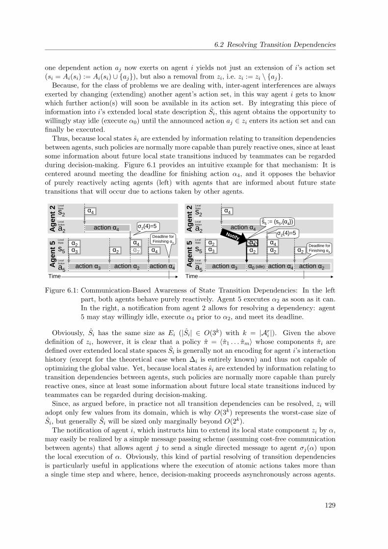
6.2 Resolving Transition Dependencies
one dependent action aj now exerts on agent i yields not just an extension of i’s action set(si = Ai(si) := Ai(si) ∪ aj), but also a removal from zi, i.e. zi := zi \ aj.
Because, for the class of problems we are dealing with, inter-agent interferences are alwaysexerted by changing (extending) another agent’s action set, in this way agent i gets to knowwhich further action(s) will soon be available in its action set. By integrating this piece ofinformation into i’s extended local state description Si, this agent obtains the opportunity towillingly stay idle (execute α0) until the announced action aj ∈ zi enters its action set and canfinally be executed.
Thus, because local states si are extended by information relating to transition dependenciesbetween agents, such policies are normally more capable than purely reactive ones, since at leastsome information about future local state transitions induced by teammates can be regardedduring decision-making. Figure 6.1 provides an intuitive example for that mechanism: It iscentered around meeting the deadline for finishing action α4, and it opposes the behaviorof purely reactively acting agents (left) with agents that are informed about future statetransitions that will occur due to actions taken by other agents.
Ag
ent
2A
gen
t 5
Time
LocalState
LocalState
LocalAction
LocalAction
s2
a2
s5
a5
α4
α2α3
action α3
action α4
α2 α2
α4
action α2
α4
σ2(4)=5
action α4
Deadline forFinishing α4
Ag
ent
2A
gen
t 5
Time
action α3
action α4
α4α2
σ2(4)=5
α2α3
α4
α2
α4α2
α0 (idle)
Deadline forFinishing α4
action α2
s5 := (s5,α4)
action α4
LocalState
LocalState
LocalAction
LocalAction
s2
a2
s5
a5
^
Notify
Figure 6.1: Communication-Based Awareness of State Transition Dependencies: In the leftpart, both agents behave purely reactively. Agent 5 executes α2 as soon as it can.In the right, a notification from agent 2 allows for resolving a dependency: agent5 may stay willingly idle, execute α4 prior to α2, and meet its deadline.
Obviously, Si has the same size as Ei (|Si| ∈ O(3k) with k = |Ari |). Given the abovedefinition of zi, however, it is clear that a policy π = 〈π1 . . . πm〉 whose components πi aredefined over extended local state spaces Si is generally not an encoding for agent i’s interactionhistory (except for the theoretical case when ∆i is entirely known) and thus not capable ofoptimizing the global value. Yet, because local states si are extended by information relating totransition dependencies between agents, such policies are normally more capable than purelyreactive ones, since at least some information about future local state transitions induced byteammates can be regarded during decision-making.
Since, as argued before, in practice not all transition dependencies can be resolved, zi willadopt only few values from its domain, which is why O(3k) represents the worst-case size ofSi, but generally Si will be sized only marginally beyond O(2k).
The notification of agent i, which instructs him to extend its local state component zi by α,may easily be realized by a simple message passing scheme (assuming cost-free communicationbetween agents) that allows agent j to send a single directed message to agent σj(α) uponthe local execution of α. Obviously, this kind of partial resolving of transition dependenciesis particularly useful in applications where the execution of atomic actions takes more thana single time step and where, hence, decision-making proceeds asynchronously across agents.
129
6 Communicating Agents and Optimal Schedules
Under those conditions, up to half of the dependencies in ∆i (over all i) may be resolved.For completeness, we also provide a formal definition of a policy that allows for partial
transition dependency resolvings via communication:
Definition 6.4 (Communication-Based Policy).For a factored m-agent DEC-MDP with changing action sets and partially ordered transitiondependencies, a communication-enhanced policy πc = 〈πc1 . . . πcm〉 consists of m local policieswith πci : Si → Ai that are defined over the extended state space Si where for all si ∈ Si itholds si = (si, zi) with si ∈ P(Ari ) and zi ∈ P(Ari \ si). For each agent i the contents of zi isdefined to be determined by messages coming from other agents j ∈ Ag \ i.
For legibility, we have defined all policies in Definitions 6.1, 6.2, and 6.4 to be deterministicones. Of course, redefining them as stochastic policies (e.g. as required for applying the JEPSor GDPS algorithm) is easily possible which we will show exemplarily below. What mattersare basically the differences in the local state spaces (Si, Ei, or Si) and action spaces (Ari orAi) over which they are defined.
Integration with JEPS, GDPS, and OA-NFQ
The communication-based approach to partially resolving state transition dependencies canbe easily combined with all learning methods that are in the center of our interest. Essentially,we require each agent j that executes an action α ∈ Arj to send a single directed message toagent i := σj(α) (σj denotes agent j’s dependency function according to Definition 2.13), thusnotifying agent i that its local state will soon be changed due to the influence of agent j. Uponreceiving this information, agent i changes its local state from (si, zi) ∈ Si to (si, zi ∪ α) ∈Si. What is more important, however, is that when executing an action (hence, starting anoperation of a job in the job-shop scheduling domain), agent i
• may either select an action α′ ∈ si in the usual manner,
• but may also pick an action α′′ ∈ zi which has been announced to become available soon,but which is currently not yet executable. In this case, agent i executes in fact the idleaction α0 until the announced action α′′ truly enters its action set (i.e. α′′ ∈ si), andthen immediately continues with the “real” execution of α′′.
Summing up, we might say that the suggested communication scheme with its correspondingcommunication-enhanced policy make the learning agents act in a reactive manner – however,reactivity is here defined over an extended local state space and also enables the usage of theidle action. The latter point is of importance with respect to the generation of schedules frombeyond the class of non-delay schedules.
Working with stochastic policies as done, for example, for GDPS, we define the stochasticcommunication-enhanced local policy by
πcθi(si, α) =
e−θ
iαP
x∈sie−θ
ix+
Px∈zi
e−θix
if α ∈ si ∪ zi
0 else(6.1)
for all α ∈ Ari and extended local states si = (si, zi) ∈ Si which depicts an extension of theGibbs policy provided in Definition 4.12. If, however, an element α ∈ zi is selected during
130
6.3 Empirical Evaluation
execution given the probabilities defined by πcθi
, then in fact agent i remains idle, i.e. it executesα0, until α enters its local state si, and after this immediately continues to process α. To whichextend this approach brings about improvements when compared to purely reactively actingagents shall be explored with the help of empirical experiments in the domain of job-shopscheduling that we present next.
Regarding the use of limited inter-agent communication in order to overcome the agents’limitation of being capable of generating non-delay schedules only, it must be acknowledgedthat this enhancement brings about an aggravation of the learning problem. Since it holds |Si| |Si|, the agents must handle a clearly increased number of local states. Also, the numberof actions to be considered in each extended state is equal or larger than in its non-extendedcounterpart si. In order to be able to trade off between the goal of learning policies superior toreactive policies and the rising of the difficulty of the learning task, we employ the parameterdmax ≥ 0 already mentioned in Section 6.2.1, which stands for the maximal number of timesteps an agent is allowed to remain idle. Given the current local state si(t) = (si(t), zi(t)), agenti is allowed to execute an α ∈ zi (by executing α0 in fact) only, if the notification regardingα has announced that α enters si after maximally dmax time steps, i.e. if ∃τ > t : α ∈ si(τ)and τ − t≤dmax. This restriction can easily be realized by adapting the first case of Equation6.1 appropriately. Thus, when setting dmax = 0, we again arrive at purely reactive agents,which for job-shop scheduling problems could generate non-delay schedules only, whereas fordmax ≥ maxx∈A δ(x) (with δ denoting the operations’ durations) the communication-basedresolving of transition dependencies is fully activated. For the experiments whose results wereport in the next section, we either made use of purely reactive agents (dmax = 0) or used avalue of dmax=20.
6.3 Empirical Evaluation
The goal of this chapter’s experimental study is to investigate the influence of the two ap-proaches for overcoming the limitations of purely reactive agents that we have proposed inthe previous section. We note that we refrain from analyzing the effects of the combinationof every learning method developed with every extension approach suggested. Nevertheless,we intend to cover a meaningful selection of methodological combinations. As before, we startwith comparative experiments using the educational FT6 benchmark before we proceed withthe results obtained for a selection of larger-scaled JSSP instances.
6.3.1 Example Benchmark
In this experiment, the issue of optimality shifts into our focus. We recall that during allexperiments in this thesis that addressed the FT6 benchmark we employed reactive agents thatyielded non-delay schedules. Accordingly, the lower bound in terms of performance (measuredin terms of minimizing makespan Cmax) was at Cnd−optmax = 57 which denotes the makespanof the best non-delay schedule. Besides, we know that the true theoretical optimum for thisproblem is represented by a schedule with a makespan of Coptmax = 55, which represents a delayschedule that requires some idleness from some of the agents in order to be generated. Thus,in previous chapters we typically aimed at achieving joint policies for the team of agents thatbrought about a schedule with Cmax = 57. By contrast, a makespan of 55 is what we wouldlike to achieve now.
131
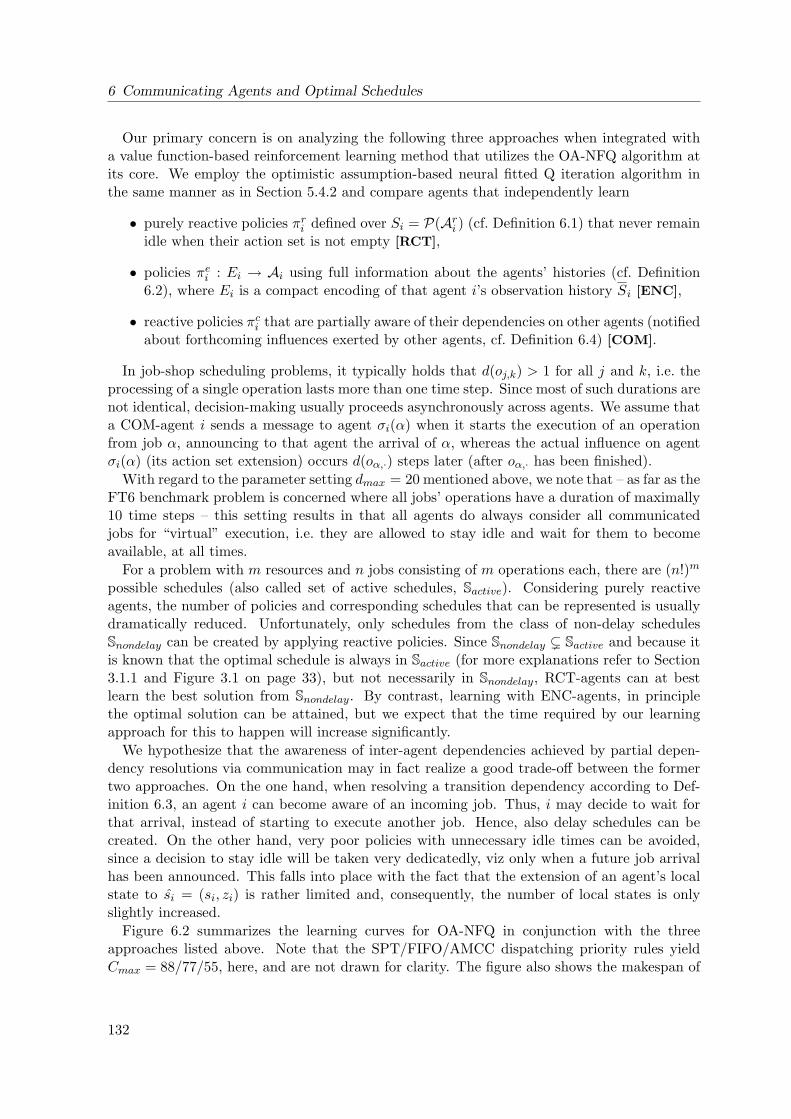
6 Communicating Agents and Optimal Schedules
Our primary concern is on analyzing the following three approaches when integrated witha value function-based reinforcement learning method that utilizes the OA-NFQ algorithm atits core. We employ the optimistic assumption-based neural fitted Q iteration algorithm inthe same manner as in Section 5.4.2 and compare agents that independently learn
• purely reactive policies πri defined over Si = P(Ari ) (cf. Definition 6.1) that never remainidle when their action set is not empty [RCT],
• policies πei : Ei → Ai using full information about the agents’ histories (cf. Definition6.2), where Ei is a compact encoding of that agent i’s observation history Si [ENC],
• reactive policies πci that are partially aware of their dependencies on other agents (notifiedabout forthcoming influences exerted by other agents, cf. Definition 6.4) [COM].
In job-shop scheduling problems, it typically holds that d(oj,k) > 1 for all j and k, i.e. theprocessing of a single operation lasts more than one time step. Since most of such durations arenot identical, decision-making usually proceeds asynchronously across agents. We assume thata COM-agent i sends a message to agent σi(α) when it starts the execution of an operationfrom job α, announcing to that agent the arrival of α, whereas the actual influence on agentσi(α) (its action set extension) occurs d(oα,·) steps later (after oα,· has been finished).
With regard to the parameter setting dmax = 20 mentioned above, we note that – as far as theFT6 benchmark problem is concerned where all jobs’ operations have a duration of maximally10 time steps – this setting results in that all agents do always consider all communicatedjobs for “virtual” execution, i.e. they are allowed to stay idle and wait for them to becomeavailable, at all times.
For a problem with m resources and n jobs consisting of m operations each, there are (n!)m
possible schedules (also called set of active schedules, Sactive). Considering purely reactiveagents, the number of policies and corresponding schedules that can be represented is usuallydramatically reduced. Unfortunately, only schedules from the class of non-delay schedulesSnondelay can be created by applying reactive policies. Since Snondelay ( Sactive and because itis known that the optimal schedule is always in Sactive (for more explanations refer to Section3.1.1 and Figure 3.1 on page 33), but not necessarily in Snondelay, RCT-agents can at bestlearn the best solution from Snondelay. By contrast, learning with ENC-agents, in principlethe optimal solution can be attained, but we expect that the time required by our learningapproach for this to happen will increase significantly.
We hypothesize that the awareness of inter-agent dependencies achieved by partial depen-dency resolutions via communication may in fact realize a good trade-off between the formertwo approaches. On the one hand, when resolving a transition dependency according to Def-inition 6.3, an agent i can become aware of an incoming job. Thus, i may decide to wait forthat arrival, instead of starting to execute another job. Hence, also delay schedules can becreated. On the other hand, very poor policies with unnecessary idle times can be avoided,since a decision to stay idle will be taken very dedicatedly, viz only when a future job arrivalhas been announced. This falls into place with the fact that the extension of an agent’s localstate to si = (si, zi) is rather limited and, consequently, the number of local states is onlyslightly increased.
Figure 6.2 summarizes the learning curves for OA-NFQ in conjunction with the threeapproaches listed above. Note that the SPT/FIFO/AMCC dispatching priority rules yieldCmax = 88/77/55, here, and are not drawn for clarity. The figure also shows the makespan of
132
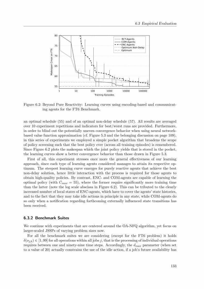
6.3 Empirical Evaluation
Figure 6.2: Beyond Pure Reactivity: Learning curves using encoding-based and communicat-ing agents for the FT6 Benchmark.
an optimal schedule (55) and of an optimal non-delay schedule (57). All results are averagedover 10 experiment repetitions and indicators for best/worst runs are provided. Furthermore,in order to blind out the potentially uneven convergence behavior when using neural network-based value function approximation (cf. Figure 5.3 and the belonging discussion on page 109),in this series of experiments we employed a simple pocket algorithm that broadens the scopeof policy screening such that the best policy ever (across all training episodes) is remembered.Since Figure 6.2 plots the makespan which the joint policy yields that is stored in the pocket,the learning curves show a better convergence behavior than those drawn in Figure 5.3.
First of all, this experiment stresses once more the general effectiveness of our learningapproach, since each type of learning agents considered manages to attain its respective op-timum. The steepest learning curve emerges for purely reactive agents that achieve the bestnon-delay solution, hence little interaction with the process is required for those agents toobtain high-quality policies. By contrast, ENC- and COM-agents are capable of learning theoptimal policy (with Cmax = 55), where the former require significantly more training timethan the latter (note the log scale abscissa in Figure 6.2). This can be tributed to the clearlyincreased number of local states of ENC-agents, which have to cover the agents’ state histories,and to the fact that they may take idle actions in principle in any state, while COM-agents doso only when a notification regarding forthcoming externally influenced state transitions hasbeen received.
6.3.2 Benchmark Suites
We continue with experiments that are centered around the OA-NFQ algorithm, yet focus onlarger-scaled JSSPs of varying problem sizes now.
For all the benchmark suites we are considering (except for the FT6 problem) it holdsδ(oj,k) ∈ [1, 99] for all operations within all jobs j, that is the processing of individual operationsrequires between one and ninety-nine time steps. Accordingly, the dmax parameter (when setto a value of 20) actually constrains the use of the idle action, if a job’s future availability has
133
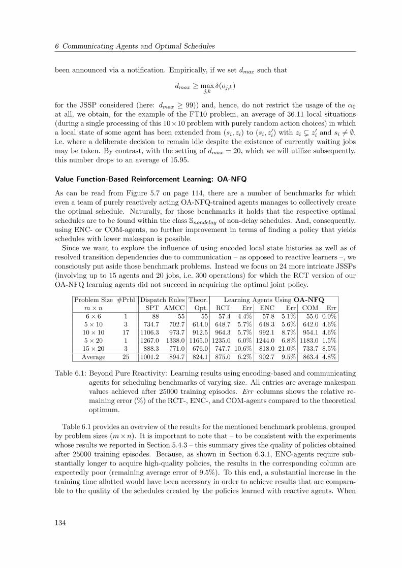
6 Communicating Agents and Optimal Schedules
been announced via a notification. Empirically, if we set dmax such that
dmax ≥ maxj,k
δ(oj,k)
for the JSSP considered (here: dmax ≥ 99)) and, hence, do not restrict the usage of the α0
at all, we obtain, for the example of the FT10 problem, an average of 36.11 local situations(during a single processing of this 10×10 problem with purely random action choices) in whicha local state of some agent has been extended from (si, zi) to (si, z′i) with zi ( z′i and si 6= ∅,i.e. where a deliberate decision to remain idle despite the existence of currently waiting jobsmay be taken. By contrast, with the setting of dmax = 20, which we will utilize subsequently,this number drops to an average of 15.95.
Value Function-Based Reinforcement Learning: OA-NFQ
As can be read from Figure 5.7 on page 114, there are a number of benchmarks for whicheven a team of purely reactively acting OA-NFQ-trained agents manages to collectively createthe optimal schedule. Naturally, for those benchmarks it holds that the respective optimalschedules are to be found within the class Snondelay of non-delay schedules. And, consequently,using ENC- or COM-agents, no further improvement in terms of finding a policy that yieldsschedules with lower makespan is possible.
Since we want to explore the influence of using encoded local state histories as well as ofresolved transition dependencies due to communication – as opposed to reactive learners –, weconsciously put aside those benchmark problems. Instead we focus on 24 more intricate JSSPs(involving up to 15 agents and 20 jobs, i.e. 300 operations) for which the RCT version of ourOA-NFQ learning agents did not succeed in acquiring the optimal joint policy.
Problem Size #Prbl Dispatch Rules Theor. Learning Agents Using OA-NFQm× n SPT AMCC Opt. RCT Err ENC Err COM Err6× 6 1 88 55 55 57.4 4.4% 57.8 5.1% 55.0 0.0%5× 10 3 734.7 702.7 614.0 648.7 5.7% 648.3 5.6% 642.0 4.6%10× 10 17 1106.3 973.7 912.5 964.3 5.7% 992.1 8.7% 954.1 4.6%5× 20 1 1267.0 1338.0 1165.0 1235.0 6.0% 1244.0 6.8% 1183.0 1.5%15× 20 3 888.3 771.0 676.0 747.7 10.6% 818.0 21.0% 733.7 8.5%Average 25 1001.2 894.7 824.1 875.0 6.2% 902.7 9.5% 863.4 4.8%
Table 6.1: Beyond Pure Reactivity: Learning results using encoding-based and communicatingagents for scheduling benchmarks of varying size. All entries are average makespanvalues achieved after 25000 training episodes. Err columns shows the relative re-maining error (%) of the RCT-, ENC-, and COM-agents compared to the theoreticaloptimum.
Table 6.1 provides an overview of the results for the mentioned benchmark problems, groupedby problem sizes (m×n). It is important to note that – to be consistent with the experimentswhose results we reported in Section 5.4.3 – this summary gives the quality of policies obtainedafter 25000 training episodes. Because, as shown in Section 6.3.1, ENC-agents require sub-stantially longer to acquire high-quality policies, the results in the corresponding column areexpectedly poor (remaining average error of 9.5%). To this end, a substantial increase in thetraining time allotted would have been necessary in order to achieve results that are compara-ble to the quality of the schedules created by the policies learned with reactive agents. When
134
6.3 Empirical Evaluation
opposing the average error yielded by RCT agents (6.2%) with the average error reported inTable 5.2 (4.4%), it must be kept in mind that the former value was determined over a differentset of benchmark problems, namely over those only for which reactively learning agents failedto acquire optimal joint policies. Accordingly, different average values are listed in these twotables.
The key observation with respect to the utilization of inter-agent communication is thatour notification scheme helps the agents in learning policies of higher quality. In terms of theaverage makespan values, a clear improvement can be achieved: While in the communication-free case the resulting schedules have an average length of 875.0 (remaining error of 6.2%), theuse of limited inter-agent notifications reduces this value to 863.4 (error of 4.8%).
Policy Search-Based Reinforcement Learning: GDPS
In Chapter 4, we have developed and evaluated different policy search RL algorithms forDEC-MDPs with changing action sets. Our empirical analysis showed a slight advantage forgradient descent policy search over joint equilibrium policy search. For this reason, in thefollowing we consider an extension of GDPS that utilizes our proposed inter-agent communi-cation mechanism and compare it to the basic (reactive and communication-free) variant ofGDPS.
Within the following series of experiments, we focus on the same selection of job-shopscheduling benchmark problems from the OR Library as in Section 4.3.5 (ranging from 5resources and 10 jobs to 15 resources and 30 jobs).
As before, for any specific m × n job-shop scheduling benchmark instance, we initialize allagents’ policies by θiα = 0 for all i ∈ 1, . . . ,m and all α ∈ Ari such that initially the agentsdispatch all waiting jobs with equal probability (such a policy, hence, represents a baseline).Recall that using the modelling and policy representation we have suggested (and assuming theJSS problem instance features no recirculations), there are n policy parameters to be storedper agent, which makes a total of mn real-valued policy parameters for the probabilistic jointpolicy. Throughout all our experiments, we allow the agents to update their local policiesbmax = 2500 times, where we use a constant learning rate β = 0.01 (cf. Equation 4.8) that hasbeen settled empirically. Estimating the gradient gα = ∇θiαJ(θi) in a Monte-Carlo manneraccording to Equation 4.13, we allot e = 100 scheduling roll-outs to be performed.
The main goal of this evaluation is to compare purely reactively learning agents with thosethat are enhanced by means of communication. As indicated above, we do so by settingdmax = 0 for reactive agents (this corresponds to the results reported in Section 4.3.5, whichwe mirror here) and by letting dmax = 20 otherwise.
Pursuing the overall goal of minimizing maximum makespan, we focus on the followingthree different evaluation criteria. First, we are interested in the makespan Cbestmax of the bestschedule that has been produced occasionally by the set of probabilistic policies during ongoinglearning. Second, we are interested in the value of the makespan Cmax(µ) of the maximumlikelihood schedule (cf. Definition 4.6 in Section 4.3.5) that arises when all of the agents selectjobs greedily, i.e. choose the action arg maxα∈Ari π
cθi
(si, α), at all decision points. Our thirdconcern is the convergence behavior and speed of the algorithm. By convergence we here referto MLS convergence as introduced in Section 4.3.5, i.e. to the number of policy updates fromwhich on the maximum likelihood schedule changes no further.
Figure 6.3 visualizes an exemplary learning run for the FT10 benchmark problem. Besidesthe development of the makespan Cmax(µ) of the maximum likelihood schedule, here also
135
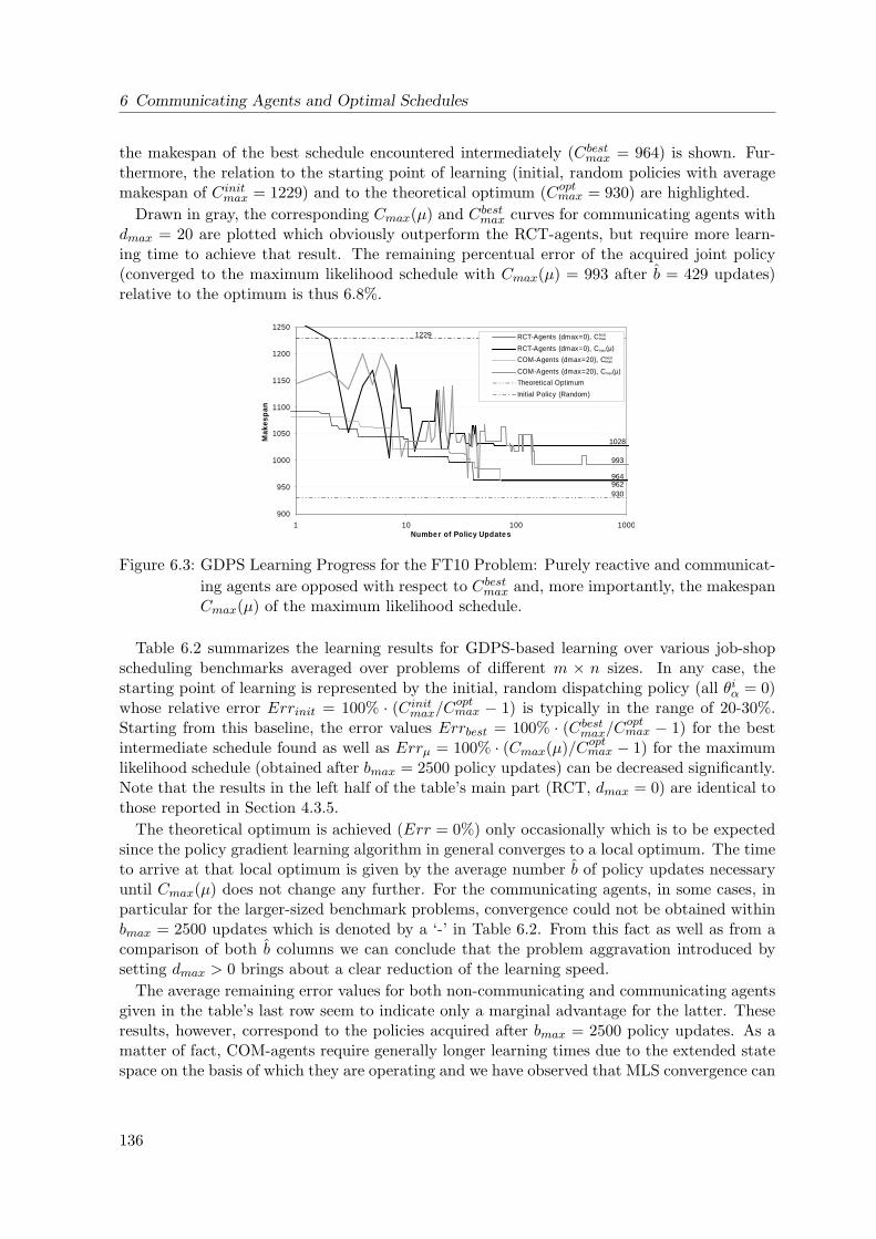
6 Communicating Agents and Optimal Schedules
the makespan of the best schedule encountered intermediately (Cbestmax = 964) is shown. Fur-thermore, the relation to the starting point of learning (initial, random policies with averagemakespan of Cinitmax = 1229) and to the theoretical optimum (Coptmax = 930) are highlighted.
Drawn in gray, the corresponding Cmax(µ) and Cbestmax curves for communicating agents withdmax = 20 are plotted which obviously outperform the RCT-agents, but require more learn-ing time to achieve that result. The remaining percentual error of the acquired joint policy(converged to the maximum likelihood schedule with Cmax(µ) = 993 after b = 429 updates)relative to the optimum is thus 6.8%.
900
950
1000
1050
1100
1150
1200
1250
1 10 100 1000Numbe r of Policy Updates
Mak
esp
an
RCT-Agents (dmax=0), C
RCT-Agents (dmax=0), C
COM-Agents (dmax=20), C
COM-Agents (dmax=20), C
Theoretical Optimum
Initial Policy (Random)
930962964
993
1028
1229max
max
max
max
best
best
(µ)
(µ)
Figure 6.3: GDPS Learning Progress for the FT10 Problem: Purely reactive and communicat-ing agents are opposed with respect to Cbestmax and, more importantly, the makespanCmax(µ) of the maximum likelihood schedule.
Table 6.2 summarizes the learning results for GDPS-based learning over various job-shopscheduling benchmarks averaged over problems of different m × n sizes. In any case, thestarting point of learning is represented by the initial, random dispatching policy (all θiα = 0)whose relative error Errinit = 100% · (Cinitmax/C
optmax − 1) is typically in the range of 20-30%.
Starting from this baseline, the error values Errbest = 100% · (Cbestmax/Coptmax − 1) for the best
intermediate schedule found as well as Errµ = 100% · (Cmax(µ)/Coptmax − 1) for the maximumlikelihood schedule (obtained after bmax = 2500 policy updates) can be decreased significantly.Note that the results in the left half of the table’s main part (RCT, dmax = 0) are identical tothose reported in Section 4.3.5.
The theoretical optimum is achieved (Err = 0%) only occasionally which is to be expectedsince the policy gradient learning algorithm in general converges to a local optimum. The timeto arrive at that local optimum is given by the average number b of policy updates necessaryuntil Cmax(µ) does not change any further. For the communicating agents, in some cases, inparticular for the larger-sized benchmark problems, convergence could not be obtained withinbmax = 2500 updates which is denoted by a ‘-’ in Table 6.2. From this fact as well as from acomparison of both b columns we can conclude that the problem aggravation introduced bysetting dmax > 0 brings about a clear reduction of the learning speed.
The average remaining error values for both non-communicating and communicating agentsgiven in the table’s last row seem to indicate only a marginal advantage for the latter. Theseresults, however, correspond to the policies acquired after bmax = 2500 policy updates. As amatter of fact, COM-agents require generally longer learning times due to the extended statespace on the basis of which they are operating and we have observed that MLS convergence can
136
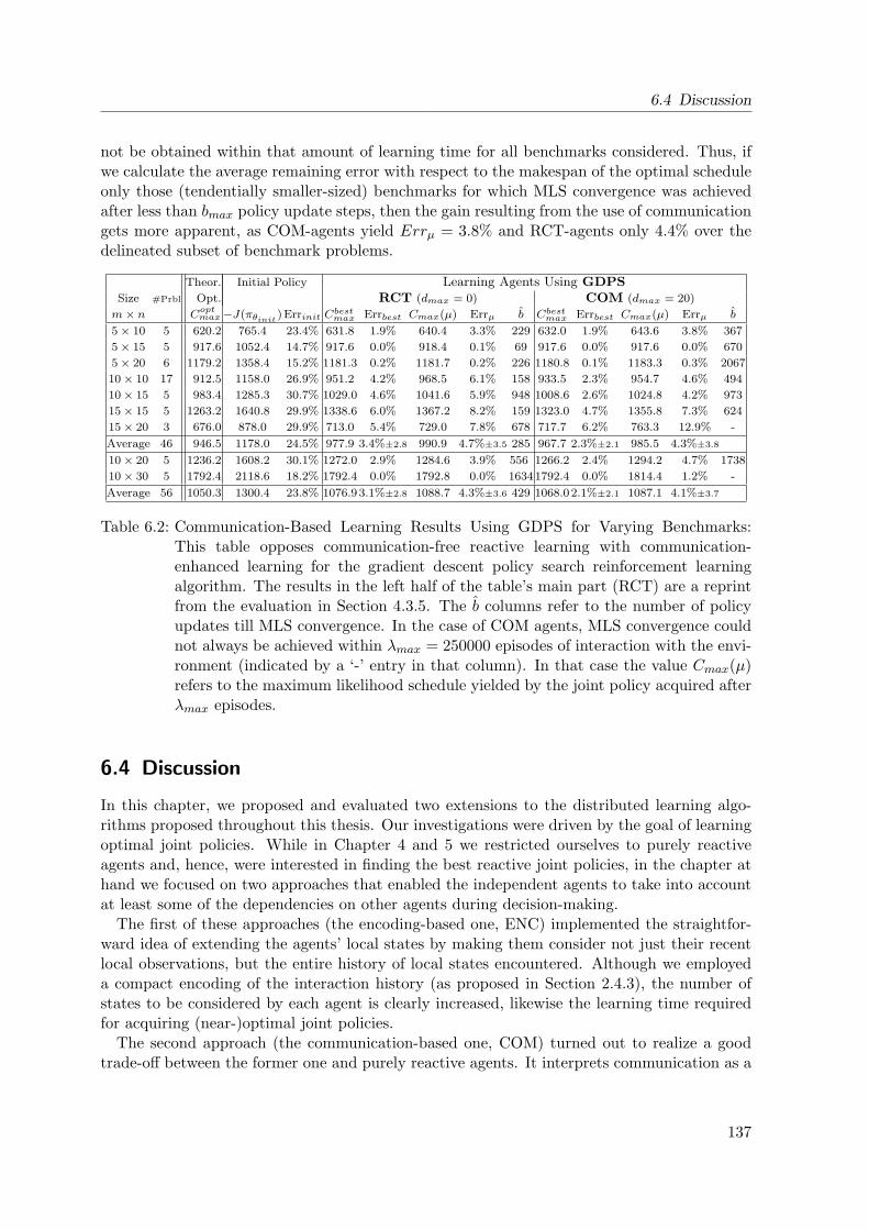
6.4 Discussion
not be obtained within that amount of learning time for all benchmarks considered. Thus, ifwe calculate the average remaining error with respect to the makespan of the optimal scheduleonly those (tendentially smaller-sized) benchmarks for which MLS convergence was achievedafter less than bmax policy update steps, then the gain resulting from the use of communicationgets more apparent, as COM-agents yield Errµ = 3.8% and RCT-agents only 4.4% over thedelineated subset of benchmark problems.
Theor. Initial Policy Learning Agents Using GDPSSize #Prbl Opt. RCT (dmax = 0) COM (dmax = 20)
m× n Coptmax−J(πθinit)Errinit C
bestmax Errbest Cmax(µ) Errµ b Cbestmax Errbest Cmax(µ) Errµ b
5× 10 5 620.2 765.4 23.4% 631.8 1.9% 640.4 3.3% 229 632.0 1.9% 643.6 3.8% 367
5× 15 5 917.6 1052.4 14.7% 917.6 0.0% 918.4 0.1% 69 917.6 0.0% 917.6 0.0% 670
5× 20 6 1179.2 1358.4 15.2% 1181.3 0.2% 1181.7 0.2% 226 1180.8 0.1% 1183.3 0.3% 2067
10× 10 17 912.5 1158.0 26.9% 951.2 4.2% 968.5 6.1% 158 933.5 2.3% 954.7 4.6% 494
10× 15 5 983.4 1285.3 30.7% 1029.0 4.6% 1041.6 5.9% 948 1008.6 2.6% 1024.8 4.2% 973
15× 15 5 1263.2 1640.8 29.9% 1338.6 6.0% 1367.2 8.2% 159 1323.0 4.7% 1355.8 7.3% 624
15× 20 3 676.0 878.0 29.9% 713.0 5.4% 729.0 7.8% 678 717.7 6.2% 763.3 12.9% -
Average 46 946.5 1178.0 24.5% 977.9 3.4%±2.8 990.9 4.7%±3.5 285 967.7 2.3%±2.1 985.5 4.3%±3.8
10× 20 5 1236.2 1608.2 30.1% 1272.0 2.9% 1284.6 3.9% 556 1266.2 2.4% 1294.2 4.7% 1738
10× 30 5 1792.4 2118.6 18.2% 1792.4 0.0% 1792.8 0.0% 16341792.4 0.0% 1814.4 1.2% -
Average 56 1050.3 1300.4 23.8% 1076.93.1%±2.8 1088.7 4.3%±3.6 429 1068.02.1%±2.1 1087.1 4.1%±3.7
Table 6.2: Communication-Based Learning Results Using GDPS for Varying Benchmarks:This table opposes communication-free reactive learning with communication-enhanced learning for the gradient descent policy search reinforcement learningalgorithm. The results in the left half of the table’s main part (RCT) are a reprintfrom the evaluation in Section 4.3.5. The b columns refer to the number of policyupdates till MLS convergence. In the case of COM agents, MLS convergence couldnot always be achieved within λmax = 250000 episodes of interaction with the envi-ronment (indicated by a ‘-’ entry in that column). In that case the value Cmax(µ)refers to the maximum likelihood schedule yielded by the joint policy acquired afterλmax episodes.
6.4 Discussion
In this chapter, we proposed and evaluated two extensions to the distributed learning algo-rithms proposed throughout this thesis. Our investigations were driven by the goal of learningoptimal joint policies. While in Chapter 4 and 5 we restricted ourselves to purely reactiveagents and, hence, were interested in finding the best reactive joint policies, in the chapter athand we focused on two approaches that enabled the independent agents to take into accountat least some of the dependencies on other agents during decision-making.
The first of these approaches (the encoding-based one, ENC) implemented the straightfor-ward idea of extending the agents’ local states by making them consider not just their recentlocal observations, but the entire history of local states encountered. Although we employeda compact encoding of the interaction history (as proposed in Section 2.4.3), the number ofstates to be considered by each agent is clearly increased, likewise the learning time requiredfor acquiring (near-)optimal joint policies.
The second approach (the communication-based one, COM) turned out to realize a goodtrade-off between the former one and purely reactive agents. It interprets communication as a
137
6 Communicating Agents and Optimal Schedules
very scarce resource, makes very dedicated use of notifications exchanged between the agents,and allows the learners to partially get to know future incoming jobs (i.e. actions that willbecome available) such that they are enabled to willingly remain idle and, hence, are capable ofcreating solutions corresponding to delay schedules. Our experiments in the scope of which, asbefore, we interpreted job-shop scheduling problems as decentralized Markov decision processeswith changing action sets and partially ordered transition dependencies confirmed that bothapproaches suggested are capable of improving the learning agents’ joint performance.
Related Work
The notification scheme that we have suggested in the scope of this chapter has turned out tobe a straightforward and effective technique for enhancing the capabilities of purely reactivelyacting agents. In so doing, we touched the issue of communication only briefly as our COM-agents make a very limited and dedicated use of this instrument, exploiting the structuralproperties and dependencies that exist in the scope of DEC-MDPs with changing action setsand partially ordered transition dependencies. As far as our learning algorithms are concerned,the restricted use of communication is convenient as, especially in practice, the establishmentof communication must be assumed to come along with some costs.
The topic of inter-agent communication has been frequently addressed in the literature onresearch on learning and coordination in multi-agent systems. A very natural approach tocommunication is to allow all agents to continually broadcast their local states to all team-mates. In the case of decentralized MDPs, this essentially renders the problem an MMDP, aseach agent gets aware of the global system state at all times. When imposing the restrictionthat such communication is allowed only every k time steps, we arrive at the DEC-POMDP-based framework of synchronizing communication by Becker et al. (2005). In contrast toBernstein’s DEC-POMDP framework, the COM-MTDP framework for modelling multi-agentproblems (Pynadath and Tambe, 2002b) contains communicative actions at its heart. It hasbeen employed to enable learning agents to willingly decide to communicate by interpretingcommunication as an additional action whose meaningful utilization must be learned (Nairet al., 2004). Similarly, in an early work, Xuan et al. (2001) define communicative acts as cen-tral elements in their framework for distributed control, and Goldman and Zilberstein (2003)define the DEC-POMDP-COM framework in which the explicit learning of communicationdecisions is targeted. However, as shown by Goldman and Zilberstein (2004), the explicit con-sideration of communication in the modelling of distributed decision problems does not bringabout more representational power.
Another interesting line of research deals with the learning of the semantics of sent messages.While transmitting local states, experience tuples, or value function estimates requires theagents involved to speak the same language, here the communication partners additionally haveto learn and recognize the meaning of messages received (Spaan et al., 2006). By contrast,in this chapter we have coped with a message passing scheme that utilizes communicationas a scarce resource and whose meaning is fixed. Thus, our work is more related to theresearch of Szer and Charpillet (2004) who enforce coordination in MMDPs using a fixed utility-based communication strategy, to the work by Aras et al. (2004) and Schneider et al. (1999)who let the agents exchange local rewards and do Q updates depending on communicatedrewards of neighboring agents, as well as to the research by Riedmiller et al. (2000) who permitcommunication between neighboring agents only, but also allow for learning to communicateand to react to received messages.
138
7 Conclusion
Decision-making in cooperative multi-agent systems has emerged as an important topic ofresearch in artificial intelligence. In distributed systems, coordinated cooperation betweenindividually acting agents is of crucial importance if it is desired to accomplish a certaincommon goal. The behavior policies of individually acting agents must be well-aligned withone another in order to achieve this. In this spirit, the focus of the thesis at hand has beenlaid on multi-agent reinforcement learning methods which allow for automatically acquiringcooperative policies based solely on a specification of the desired joint behavior of the wholesystem.
Likewise, many larger-scale applications are well-suited to be formulated in terms of spatiallyor functionally distributed entities, i.e. using a multi-agent approach. One such applicationarea is represented by production planning and optimization problems. To this end, ourparticular interest has been on distributed job-shop scheduling problems which are known to becomputationally very difficult and which naturally allow for decentralized solution approaches.
7.1 Summary
The research described in this dissertation has been conducted along three complementarylines and has thus brought about contributions within three different, yet related areas.
Modelling of Distributed Decision-Making Problems
Research on distributed control of cooperative multi-agent systems has received a lot of at-tention during the past years. While Markov decision processes (MDP) have proven to be asuitable tool for solving problems involving a single agent, a number of extensions of thesemodels to multi-agent systems have been suggested. Among those, the DEC-MDP framework(Bernstein et al., 2002), that is characterized by each agent having only a partial view ofthe global system state, has been frequently investigated. However, it has been shown thatthe complexity of general DEC-MDPs is NEXP-complete, even for the benign case of twocooperative agents.
In this regard, a first contribution of this thesis is that we have identified a class of cooperativedecentralized MDPs that features a number of regularities in the way agents influence the statetransitions of other agents (Section 2.4). Exploiting the knowledge about these correlations,we have proven that this class of problems – called factored m-agent decentralized Markovdecision processes with changing action sets and partially ordered transition dependencies – iseasier to solve (NP-hard) than general DEC-MDPs (NEXP-hard).
Interestingly, this subclass of DEC-MDPs covers a wide range of practical problems. In prac-tice, distributed problem-solving is often characterized by a larger number of agents involvedand by a factored system state description where the agents base their decisions on local ob-servations. Also, the assumptions we made, namely that local actions may influence the statetransitions of maximally one other agent and that any action has to be performed only once,
139
7 Conclusion
are frequently fulfilled. Sample real-world applications include scenarios from manufacturing,production planning, or assembly line optimization, where typically the production of a goodinvolves a number of processing steps that have to be performed in a specific order and wherean appropriate scheduling of single operations is crucial to maximize joint productivity. Wehave shown that our class of factored m-agent DEC-MDPs with changing action sets andpartially ordered transition dependencies covers a various scheduling problems, for exampleflow-shop and job-shop scheduling scenarios (Pinedo, 2002), even scheduling problems withrecirculating tasks can be modelled.
Model-Free Multi-Agent Reinforcement Learning Algorithms
Despite the mitigation in terms of reduced problem complexity just summarized, the class ofdecentralized problems we have been focusing on is NP-hard. Accordingly, it has not been ourgoal to develop new optimal solution algorithms which would be doomed by computationalintractability with growing problem sizes. Instead, we have tackled distributed decision-makingproblems by utilizing model-free reinforcement learning techniques. When employing thesetechniques, we interpret the agents as being independent adaptive entities that learn to improvetheir behavior by trial and error-based interaction with the environment. Based on this ideaof decentralized model-free learning, we have developed three novel multi-agent reinforcementlearning algorithms.
On the one hand, in Chapter 4, we have proposed two policy search-based reinforcementlearning algorithms that are geared to finding near-optimal joint policies for the agents withinthe DEC-MDP.
• Joint equilibrium policy search (JEPS, Section 4.2) turned out to be an effective methodfor enforcing coordination between the agents in order to achieve optimal joint policiesor good approximations thereof. Furthermore, an enhanced variant of this algorithmadheres to a number of nice theoretical convergence guarantees.
• Policy gradient methods have recently gained much popularity within the RL and dis-tributed AI community. So, as a second implementation of a policy search-based RLapproach, we have shown how to apply a gradient-descent policy search (GDPS, Section4.3) method to distributed problems. Although policy gradient algorithms generallydo not allow for finding the best joint policy, they facilitate discovering near-optimalapproximations, as represented by local optima in the search space, within little time.
On the other hand, we have utilized the more traditional, i.e. value function-based approachto reinforcement learning for the problem settings of our interest (Chapter 5). Additionally,we have aimed at learning agent-specific policies that feature good generalization capabilities,meaning that they should be applicable to problem instances not covered during the learningprocess and that, hence, incorporate general problem knowledge.
• To this end, we have presented a new distributed RL algorithm for learning in determinis-tic multi-agent environments, optimistic assumption-based neural fitted Q iteration (OA-NFQ). This algorithm realizes a combination of data-efficient batch-mode reinforcementlearning in conjunction with neural value function approximation, and the utilization ofan optimistic inter-agent coordination.
140
7.2 Outlook
It makes quite a difference whether an agent in a DEC-MDP makes its local decisions basedsolely on its most recent local observation, i.e. in a purely reactive, memoryless manner, orwhether it remembers its entire history of interaction with the environment and, thus, withother agents. Alternatively, other agents may be endowed to reveal, for example via com-munication, some of their local information to teammates so as to attenuate the potentiallydetrimental effects of inter-agent dependencies. We have studied these issues in the preced-ing chapter of this thesis, essentially proposing a limited inter-agent notification scheme forDEC-MDPs with changing action sets and empirically confirming the benefits of explicitlyconsidering and resolving inter-agent dependencies.
Application for Distributed Job-Shop Scheduling Problems
A third, and final line of research embedded in this dissertation has dealt with the application ofthe proposed modelling approaches and learning algorithms to distributed job-shop schedulingproblems.
Job-shop problems are NP-hard. In contrast to classical analytical scheduling approaches,we have pursued an alternative approach to scheduling, where each resource is assigned adecision-making agent that decides which job to process next, based on its partial view of theproduction plant. More specifically, we have shown how scheduling problems can be cast (andsubsequently solved) as decentralized Markov decision processes and how this matches withthe subclass of general DEC-MDPs identified before.
Although it is possible to adopt a global view on a given scheduling problem – as is donein analytical scheduling –, to model it as a single MDP, we preferred to interpret and solveit as a multi-agent learning problem using our learning approach relying on reinforcementlearning. On the one hand, we therefore arrive at the challenge of a problem complicationdue to independently learning agents. But, on the other hand, we derive the benefit of beingenabled to perform reactive scheduling, including the capability to react to unforeseen events.Furthermore, a decentralized view on a scheduling task is of higher relevance to practice sincea central control cannot always be instantiated.
We have turned to a variety of established job-shop scheduling benchmark problems forthe purpose of validating and evaluating the performance of all learning algorithms proposedthroughout this thesis. Despite certain restrictions of these algorithms, as well as approxi-mations introduced by these methods, the empirical parts within the methodological chapters(Chapters 4-6) contain several convincing results for classical Operations Research job-shopscheduling benchmarks. Our experiments for such large-scale benchmark problems let us comeup with the conclusion that problems of current standards of difficulty can very well be effec-tively solved by the learning method we suggest: The dispatching policies our learning agentsacquire clearly surpass traditional dispatching rules and, in some cases, are able to reach thetheoretically optimal solution. Notwithstanding the inherent difficulties in facing partial stateobservability and agent independent learning, the dispatching policies acquired do also gener-alize to unknown situations without retraining, i.e. they are adequate for similar schedulingproblems not covered during the learning phase.
7.2 Outlook
The work performed and described in the scope of this thesis opens a number of opportunitiesfor interesting directions of future research. In this section, we concentrate on both possible
141
7 Conclusion
extensions of our work as well as on alternative research directions.
Applicability and Stochasticity
In Chapter 3, we have shown that the class of decentralized problems identified in Section 2.4and focused on subsequently matches well with job-shop scheduling problems. We have alsopointed to the fact that this class’ usability is not restricted to this application area, but canbe employed for different scheduling problems and application domains beyond manufacturingas well. Accordingly, an interesting avenue for future work is represented by employing andassessing the learning algorithms developed to different tasks, e.g. to network routing or trafficcontrol problems.
Classical job-shop scheduling problems (cf. Section 3.1), which we used throughout thisthesis as benchmark, are deterministic in nature. There are also stochastic versions of job-shop scheduling problems (Pinedo, 2002). Stochasticity may arise, for example, if the durationsof a job’s operations are randomly perturbed or if (adopting a practice-oriented perspective)the execution of some operation to some product has failed, thus requiring a repetition ofthat operation. We stress once more that our modelling framework allows for stochasticityby definition. The distributed learning algorithms we have suggested do so in part: WhileGDPS is immediately applicable to stochastic JSSPs (see Gabel and Riedmiller (2008b) forcorresponding experimental results), the versions of JEPS proposed in this document are not,because of their straightforward implementation of the heuristic function (we elaborate moreon this point below). OA-NFQ requires a deterministic environment during learning in orderto fully exploit the power of the optimistic assumption it uses, whereas NFQ is not bothered bya stochastic environment. Both of these value function-based RL algorithms can handle non-determinism in their application phase, i.e. when exploiting their learned dispatching policiesfor some new scheduling problem. Although we did not explicitly test these algorithms forstochastic JSS problems, we in fact challenged them even more by testing the acquired jointpolicies for entirely different scheduling problem instances (not just for noisified ones). After all,however, the further development of those components of the learning approaches mentionedthat prohibit their use in stochastic systems (e.g. the optimistic assumption or JEPS’ heuristicfunction implementation) represents a major and very interesting challenge for future work.
Extensions and Alternatives
In Chapter 4, we have applied our policy search-based RL solution approaches consistentlywith constant learning rates. However, adaptive methods exist (e.g. the Rprop method, Ried-miller and Braun, 1993) that allow for dynamically changing learning rate vectors as learningproceeds. As such adaptations typically result in a significant speed-up of the learning progress(Kocsis et al., 2006), a combination of JEPS and GDPS with Rprop is a promising idea.
Such a speed-up may be very desirable, especially if an extension of the proposed policysearch methods towards the consideration of interaction histories, and hence the considerationof much larger state spaces, is desired. The latter represents a promising idea in itself since,as shown theoretically in Section 2.4 and empirically in Section 6.3, memory-based learningagents have a clear advantage over memoryless ones, although this extension will significantlyincrease the amount of experience to be collected through interaction with the environment.
Another important issue for future work concerns particularly the JEPS algorithm (Section4.2). We have investigated its theoretical properties, assuming the existence of an optimal
142
7.2 Outlook
heuristic function H that tells whether a joint equilibrium has been attained. In practice, ofcourse, an optimal heuristic cannot be expected to be known and, in fact, for our experimentsaround JEPS we employed a straightforward, Rmax-based implementation of H. To this end,the performance of JEPS can supposedly be improved if more sophisticated realizations ofthe heuristic are utilized. For instance, the explorative capabilities of JEPS may be increasedif an ε-Rmax-based heuristic with vanishing ε is used, that returns true if the current policyperformance is within an ε-vicinity of Rmax.
In the context of the experiments around our OA-NFQ approach, we have also comparedlocal and global reward schemes. While the former allow for a higher degree of decentralizationof the entire learning process, they enforce selfish agent behavior and yield a poor degree ofcooperation. Concerning job-shop scheduling using cooperative agents, global rewards obvi-ously brought about best performance. But, using the notion of Tumer and Agogino (2004),such reward functions feature a high degree of learnability and, at the same time, a low fac-toredness. To this end, it would be an interesting idea to integrate and analyze different utilityfunctions, such as the wonderful life utility scheme (Tumer et al., 2002).
With respect to our value function-based approaches (Chapter 5), we invested a moderateeffort in the task of feature engineering, i.e. in finding and crafting comprehensive and gen-eral features that describe individual actions (in our JSS application: available jobs) or localstates (sets of waiting jobs). There exist, however, powerful mechanisms that aid the systemdesigner in creating or removing certain features (Guyon and Elisseeff, 2003). Hence, the useof state-of-the-art feature engineering methods, such as clustering methods, singular value de-composition, or principal component analysis, may enhance the applicability and performance,and eventually even the already excellent generalization capabilities of our learning approach.
In our model-free batch-mode reinforcement learning algorithms (Sections 5.2 and 5.3), wefocussed on the use of artificial neural networks as a tool for approximating value functionsover high-dimensional continuous state-action spaces in the context of the fitted Q iterationalgorithm. Of course, there are also other powerful machine learning algorithms that mightbe employed for this purpose, for example, decision trees (Ernst et al., 2006), support vectorregression (Csaji and Monostori, 2008), or Gaussian processes (Deisenroth et al., 2008). Acomparison of NFQ and OA-NFQ against FQI variants using other function approximationmechanisms depicts a further interesting topic.
Multi-layer perceptron neural networks are well-known for their representational power,their good generalization capabilities, and, when used in batch-mode, for their combinabilitywith advanced network training methods. A drawback when using them in the scope ofvalue function-based RL is their lack of convergence guarantees (Gordon, 1996). In order toenforce stable learning results, we relied on the straightforward, but computationally expensivepolicy screening technique (Bertsekas et al., 2000) which selects high-quality policies in spiteof oscillations in the learning process. Research on more efficient methods that foster robustlearning behavior for neural value function-based RL depicts an important open issue.
Finally, we have employed a restricted inter-agent notification scheme to enable the learningagents to resolve some of their dependencies on one another. While this turned out to be ahighly effective and efficient approach, another interesting direction is to study the learning ofwhen and with whom to communicate (Riedmiller et al., 2000), given that communication isno longer free of charge, but modelled as an action that incurs some cost.
143

7 Conclusion
144
Glossary
AI Artificial IntelligenceAMCC Avoid maximum current makespanCOM-MTDP Communicating multi-agent team decision problemDEC-MDP Decentralized Markov decision processDEC-POMDP Decentralized partially observable Markov decision processDPR Dispatching priority ruleFIFO First in first outFQI Fitted Q iterationFT6, FT10 Job-shop scheduling benchmark problem instances proposed
by Fisher and Thompson (Muth and Thompson, 1963)GDPS Gradient-descent policy searchIL Independent learnerIPL Incremental policy learningJAL Joint-action learnerJEPS Joint equilibrium policy searchJSS Job-shop schedulingJSSP Job-shop scheduling problemLPT Longest processing timeMDP Markov decision processMLP Multi-layer perceptronMLS Maximum likelihood scheduleMMDP Multi-agent Markov decision processNEXP Complexity class of problems solvable in exponential time by a
non-deterministic Turing machineNFQ Neural fitted Q iterationNP Complexity class of problems solvable in polynomial time by a
non-deterministic Turing machineOA-NFQ Optimistic assumption-based neural fitted Q iterationP Complexity class of problems solvable in polynomial time by a
Deterministic Turing machinePG Policy gradientPOIPSG Partially observable identical payoff stochastic gamePOMDP Partially observable Markov decision processPOSG Partially observable stochastic gamePSPACE Complexity class of problems solvable in by a deterministic Turing
machine with polynomial space requirementsRL Reinforcement learningSPT Shortest processing timeSQNO Shortest queue for next operationTD Temporal difference
145

Bibliography
D. Aberdeen and O. Buffet. Concurrent Probabilistic Temporal Planning with Policy-Gradients. In Proceedings of the Seventeenth International Conference on Automated Plan-ning and Scheduling (ICAPS 2007), pages 10–17, Providence, USA, 2007. AAAI Press.
J. Adams, E. Balas, and D. Zawack. The Shifting Bottleneck Procedure for Job Shop Schedul-ing. Management Science, 34(3):391–401, 1988.
A. Agogino and K. Tumer. Multi-agent Reward Analysis for Learning in Noisy Domains. InProceedings of the 4th International Joint Conference on Autonomous Agents and MultiagentSystems (AAMAS 2005), pages 81–88, Utrecht, The Netherlands, 2005. ACM Press.
C. Amato, D. Bernstein, and S. Zilberstein. Optimizing Memory-Bounded Controllers forDecentralized POMDPs. In Proceedings of the 23rd Conference on Uncertainty in ArtificialIntelligence (UAI 2007), Vancouver, Canada, 2007.
D. Applegate and W. Cook. A Computational Study of the Job-Shop Scheduling Problem.ORSA Journal on Computing, 3:149–156, 1991.
R. Aras, A. Dutech, and F. Charpillet. Cooperation through Communication in DecentralizedMarkov Games. In Proceedings of the International Conference on Advances in IntelligentSystems – Theory and Applications (AISTA 2004), Luxembourg, Luxembourg, 2004. IEEEPress.
K. Arrow and L. Hurwicz. Stability of the Gradient Process in n-Person Games. Journal ofthe Society of Industrial and Applied Mathematics, 8(2):280–295, 1960.
M. Aydin and E. Oztemel. Dynamic Job-Shop Scheduling Using Reinforcement LearningAgents. Robotics and Autonomous Systems, 33:169–178, 2000.
J. Bagnell and A. Ng. On Local Rewards and Scaling Distributed Reinforcement Learning. InAdvances in Neural Information Processing Systems 18 (NIPS 2005), Vancouver, Canada,2005.
L. Baird and A. Moore. Gradient Descent for General Reinforcement Learning. In Advancesin Neural Information Processing Systems 11 (NIPS 1998), pages 968–974, Denver, USA,1999. The MIT Press.
A. Baker. A Survey of Factory Control Algorithms which Can Be Implemented in a Multi-Agent Heterarchy: Dispatching, Scheduling, and Pull. Journal of Manufacturing Systems,17(4):297–320, 1998.
A. Barto and R. Crites. Improving Elevator Performance using Reinforcement Learning. In Ad-vances in Neural Information Processing Systems 8 (NIPS 1995), pages 1017–1023, Denver,USA, 1996. MIT Press.
147
Bibliography
A. Barto, R. Sutton, and C. Anderson. Neuron-Like Elements that Can Solve Difficult LearningControl Problems. IEEE Transactions on Systems, Man, and Cybernetics, 13:835–846, 1983.
J. Baxter and P. Bartlett. Direct Gradient-Based Reinforcement Learning: I. Gradient Estima-tion Algorithms. Technical report, Research School of Information Sciences and Engineering,Australian National University, 1999.
J. Bean. Genetics and Random Keys for Sequencing and Optimization. ORSA Journal ofComputing, 6:154–160, 1994.
J. Beasley. OR-Library, 2005.http://people.brunel.ac.uk/∼mastjjb/jeb/info.html.
R. Becker, S. Zilberstein, and V. Lesser. Decentralized Markov Decision Processes with Event-Driven Interactions. In Proceedings of the 3rd International Conference on AutonomousAgents and Multi-Agent Systems (AAMAS 2004), pages 302–309, New York, USA, 2004a.ACM Press.
R. Becker, S. Zilberstein, V. Lesser, and C. Goldman. Solving Transition Independent Decen-tralized MDPs. Journal of Artificial Intelligence Research, 22:423–455, 2004b.
R. Becker, V. Lesser, and S. Zilberstein. Analyzing Myopic Approaches for Multi-Agent Com-munication. In Proceedings of the 2005 IEEE/WIC/ACM International Conference on In-telligent Agent Technology (IAT 2005), pages 550–557, Compiegne, France, 2005. IEEEComputer Society.
R. E. Bellman. Dynamic Programming. Princeton University Press, USA, 1957.
D. Bernstein, R. Givan, N. Immerman, and S. Zilberstein. The Complexity of DecentralizedControl of Markov Decision Processes. In Proceedings of the 16th Conference in Uncer-tainty in Artificial Intelligence (UAI’00), pages 32–37, Stanford, CA, June 2000. MorganKaufmann.
D. Bernstein, D. Givan, N. Immerman, and S. Zilberstein. The Complexity of DecentralizedControl of Markov Decision Processes. Mathematics of Operations Research, 27(4):819–840,2002.
D. Bernstein, E. Hansen, and S. Zilberstein. Bounded Policy Iteration for DecentralizedPOMDPs. In Proceedings of the 19th International Joint Conference on Artificial Intel-ligence (IJCAI 2005), pages 1287–1292, Edinburgh, United Kingdom, 2005. ProfessionalBook Center.
D. Bertsekas and J. Tsitsiklis. Neuro Dynamic Programming. Athena Scientific, Belmont,USA, 1996.
D. Bertsekas, M. Homer, D. Logan, S. Patek, and N. Sandell. Missile Defense and InterceptorAllocation by Neuro-Dynamic Programming. IEEE Transactions on Systems, Man, andCybernetics, 30(1):42–51, 2000.
A. Beynier and A. Mouaddib. A Polynomial Algorithm for Decentralized Markov DecisionProcesses with Temporal Constraints. In Proceedings of the 4th International Joint Con-ference on Autonomous Agents and Multiagent Systems (AAMAS 2005), pages 963–969,Utrecht, The Netherlands, 2005. ACM Press.
148
Bibliography
A. Beynier and A. Mouaddib. An Iterative Algorithm for Solving Constrained Decentral-ized Markov Decision Processes. In Proceedings, The Twenty-First National Conference onArtificial Intelligence (AAAI 2006), Boston, USA, 2006. AAAI Press.
K. Bhaskaran and M. Pinedo. Dispatching. In G. Salvendy, editor, Handbook of IndustrialEngineering, pages 2184–2198. John Wiley, New York, USA, 1977.
B. Bikramjit, S. Sen, and J. Peng. Fast Concurrent Reinforcement Learners. In Proceedingsof the 17th International Joint Conference on Artificial Intelligence (IJCAI 2001), pages825–830, Seattle, WA, August 2001. Morgan Kaufmann.
S. Binato, W. Hery, D. Loewenstern, and M. Resende. A GRASP for Job Shop Scheduling.In P. Hansen and C. Ribeiro, editors, Essays and Surveys in Metaheuristics, pages 177–293.Kluwer Academic Publishers, New York, USA, 2001.
J. Blazewicz, K. Ecker, G. Schmidt, and J. Weglarz. Scheduling in Computer and Manufac-turing Systems. Springer, Berlin, Germany, 1993.
C. Boutilier. Sequential Optimality and Coordination in Multiagent Systems. In Proceedings of16th International Joint Conference on Artificial Intelligence (IJCAI 1999), pages 478–485,Stockholm, Sweden, 1999. Morgan Kaufmann.
D. Bovet and P. Crescenzi. Introduction to the Theory of Complexity. Prentice Hall, Hertford-shire, United Kingdom, 1994.
M. Bowling. Convergence Problems of General-Sum Multiagent Reinforcement Learning. InProceedings of the Seventeenth International Conference on Machine Learning (ICML 2000),pages 89–94, Stanford, USA, 2000. Morgan Kaufmann.
J. Boyan and M. Littman. Packet Routing in Dynamically Changing Networks – A Reinforce-ment Learning Approach. In Advances in Neural Information Processing Systems 6 (NIPS1993), pages 671–678, Denver, USA, 1994. Morgan Kaufmann.
J. A. Boyan and A. W. Moore. Generalization in Reinforcement Learning: Safely Approxi-mating the Value Function. In Advances in Neural Information Processing Systems 7, pages369–376, Cambridge, USA, 1995. MIT Press.
R. Brafman and M. Tennenholtz. Learning to Cooperate Efficiently: A Model-Based Approach.Journal of Artificial Intelligence Research, 19:11–23, 2003.
R. Brafman and M. Tennenholtz. R-MAX - A General Polynomial Time Algorithm for Near-Optimal Reinforcement Learning. In Proceedings of the 17th International Joint Conferenceon Artificial Intelligence (IJCAI 2001), pages 953–958, Seattle, USA, 2001. Morgan Kauf-mann.
P. Brucker and S. Knust. Complex Scheduling. Springer, Berlin, Germany, 2005.
P. Brucker, B. Jurisch, and B. Sievers. A Branch and Bound Algorithm for the Job-ShopScheduling Problem. Discrete Applied Mathematics, 49(1-2):107–127, 1994.
J. Carlier and E. Pinson. An Algorithm for Solving the Job-Shop Problem. ManagementScience, 35(2):164–176, 1989.
149

Bibliography
I. Chades and B. Bouteiller. Solving Multiagent Markov Decision Processes: A Forest Manage-ment Example. In Proceedings of the International Congress on Modelling and Simulation(MODSIM 2005), pages 1594–1600, Canberra, Australia, 2005. Modelling and SimulationSociety of Australia and New Zealand.
Y. Chang, T. Ho, and L. Kaelbling. All Learning Is Local: Multi-Agent Learning in GlobalReward Games. In Advances in Neural Information Processing Systems 16 (NIPS 2003),Vancouver and Whistler, Canada, 2003.
Y. Chang, T. Ho, and L. Kaelbling. Mobilized Ad-Hoc Networks: A Reinforcement LearningApproach. In Proceedings of the First International Conference on Autonomic Computing(ICAC 2004), pages 240–247, New York, USA, 2004. IEEE Computer Society.
K. Chellapilla and D. Fogel. Evolution, Neural Networks, Games, and Intelligence. Proceedingsof the IEEE, 87(9):1471–1496, 1999.
C. Claus and C. Boutilier. The Dynamics of Reinforcement Learning in Cooperative Multia-gent Systems. In Proceedings of the Fifteenth National Conference on Artificial Intelligence(AAAI-98), pages 746–752, Menlo Park, USA, 1998. AAAI Press.
B. Csaji and L. Monostori. Adaptive Stochastic Resource Control: A Machine LearningApproach. Journal of Artificial Intelligence Research, 32:453–486, 2008.
B. Csaji and L. Monostori. Adaptive Algorithms in Distributed Resource Allocation. InProceedings of the 6th International Workshop on Emergent Synthesis (IWES 2004), pages69–75, Kashiwa, Japan, 2004.
B. Csaji and L. Monostori. Adaptive Sampling Based Large-Scale Stochastic Resource Con-trol. In Proceedings of the 21st National Conference on Artificial Intelligence (AAAI 2006),Boston, USA, 2006. AAAI Press.
M. Deisenroth, J. Peters, and C. Rasmussen. Approximate Dynamic Programming with Gaus-sian Processes. In Proceedings of the 2008 American Control Conference (ACC 2008), pages4480–4485, Seattle, USA, 2008. IEEE Press.
M. Dell’Amico and M. Trubian. Applying Tabu Search to the Job-Shop Scheduling Problem.Annals of Operations Research, 41(1-4):231–252, 1993.
D. Ernst, P. Geurts, and L. Wehenkel. Tree-Based Batch Mode Reinforcement Learning.Journal of Machine Learning Research, 6(1):503–556, 2006.
H. Ferra, K. Lau, C. Leckie, and A. Tang. Applying Reinforcement Learning to Packet Schedul-ing in Routers. In Proceedings of the Fifteenth Innovative Applications of Artificial Intelli-gence Conference (IAAI-03), pages 79–84, Acapulco, Mexico, 2003. AAAI Press.
E. Ferreira and P. Khosla. Multi Agent Collaboration Using Distributed Value Functions.In Proceedings of the IEEE Intelligent Vehicle Symposium 2000 (IV 2000), pages 404–409,Dearborn, USA, 2000. IEEE Press.
J. Filar and O. Vrieze. Competitive Markov Decision Processes – Theory, Algorithms, andApplications. Springer-Verlag, New York, USA, 1996.
150
Bibliography
D. Fudenberg and J. Tirole. Game Theory. MIT Press, Boston, USA, 1991.
N. Fulda and D. Ventura. Incremental Policy Learning: An Equilibrium Selection Algorithmfor Reinforcement Learning Agents with Common Interests. In Proceedings of the 2004 IEEEInternational Joint Conference on Neural Networks (IJCNN), pages 1121–1125, Budapest,Hungary, 2004. IEEE Press.
T. Gabel and M. Riedmiller. Adaptive Reactive Job-Shop Scheduling with Learning Agents.International Journal of Information Technology and Intelligent Computing, 2(4), 2007a.
T. Gabel and M. Riedmiller. Multi-Agent Case-Based Reasoning for Cooperative Reinforce-ment Learners. In Proceedings of the 8th European Conference on Case-Based Reasoning(ECCBR 2006), pages 32–46, Fethiye, Turkey, 2006a. Springer.
T. Gabel and M. Riedmiller. Reducing Policy Degradation in Neuro-Dynamic Programming.In Proceedings of ESANN2006, pages 653–658, Bruges, Belgium, 2006b.
T. Gabel and M. Riedmiller. On a Successful Application of Multi-Agent ReinforcementLearning to Operations Research Benchmarks. In Proceedings of the IEEE Symposium onApproximate Dynamic Programming and Reinforcement Learning (ADPRL 2007), pages68–75, Honolulu, USA, 2007b. IEEE Press.
T. Gabel and M. Riedmiller. Scaling Adaptive Agent-Based Reactive Job-Shop Schedulingto Large-Scale Problems. In In Proceedings of the IEEE Symposium on ComputationalIntelligence in Scheduling (CI-Sched 2007), pages 259–266, Honolulu, USA, 2007c. IEEEPress.
T. Gabel and M. Riedmiller. Reinforcement Learning for DEC-MDPs with Changing ActionSets and Partially Ordered Dependencies. In Proceedings of the 7th International JointConference on Autonomous Agents and Multiagent Systems (AAMAS 2008), pages 1333–1336, Estoril, Portugal, 2008a. IFAAMAS.
T. Gabel and M. Riedmiller. Gradient Descent Policy Search for Distributed Job-Shop Schedul-ing Problems. In Online Proceedings of the 18th International Conference on Planning andScheduling (ICAPS 2008), Sydney, Australia, 2008b. AAAI Press.
T. Gabel and M. Riedmiller. Joint Equilibrium Policy Search for Multi-Agent SchedulingProblems. In Proceedings of the 6th Conference on Multiagent System Technologies (MATES2008), pages 61–72, Kaiserslautern, Germany, 2008c. Springer.
T. Gabel and A. Stahl. Exploiting Background Knowledge when Learning Similarity Measures.In Proceedings of the 7th European Conference on Case-Based Reasoning (ECCBR 2004),pages 169–183, Madrid, Spain, 2004. Springer.
T. Gabel, R. Hafner, S. Lange, M. Lauer, and M. Riedmiller. Bridging the Gap: Learning inthe RoboCup Simulation and Midsize League. In Proceedings of the 7th Portuguese Confer-ence on Automatic Control (Controlo 2006), Porto, Portugal, 2006. Portuguese Society ofAutomatic Control.
Chris Gaskett. Q-Learning for Robot Control. Ph.D. Thesis, Australian National University,2002.
151
Bibliography
P. Gmytrasiewicz and P. Doshi. A Framework for Sequential Planning in Multiagent Settings.Journal of Artificial Intelligence Research, 24:49–79, 2005.
C. Goldman and S. Zilberstein. Decentralized Control of Cooperative Systems: Categorizationand Complexity Analysis. Journal of Artificial Intelligence Research, 22:143–174, 2004.
C. Goldman and S. Zilberstein. Optimizing Information Exchange in Cooperative Multi-AgentSystems. In Proceedings of the Second International Conference on Autonomous Agents andMulti-Agent Systems (AAMAS 2003), pages 137–144, Melbourne, Australia, 2003. ACMPress.
M. Gonzalez, C. Vela, and R. Varela. A New Hybrid Genetic Algorithm for the Job ShopScheduling Problem with Setup Times. In Proceedings of the 18th International Conferenceon Automated Planning and Scheduling (ICAPS 2008), pages 116–123, Sydney, Australia,2008. AAAI Press.
G. Gordon. Stable Fitted Reinforcement Learning. In Advances in Neural Information Pro-cessing Systems 9 (NIPS 1995), pages 1052–1058, Denver, USA, 1996. The MIT Press.
E. Greensmith, P. Bartlett, and J. Baxter. Variance Reduction Techniques for Gradient Es-timates in Reinforcement Learning. Journal of Machine Learning Research, 5:1471–1530,2004.
A. Greenwald and K. Hall. Correlated Q-Learning. In Proceedings of the 20th InternationalConference on Machine Learning (ICML 2003), pages 242–249, Washington, USA, 2003.AAAI Press.
C. Guestrin, M. Lagoudakis, and R. Parr. Coordinated Reinforcement Learning. In Proceed-ings of 19th International Conference on Machine Learning (ICML 2002), pages 227–234,Sydney, Australia, 2002. Morgan Kaufmann.
I. Guyon and A. Elisseeff. An Introduction to Variable and Feature Selection. Journal ofMachine Learning Research, 3:1157–1182, 2003.
E. Hansen, D. Bernstein, and S. Zilberstein. Dynamic Programming for Partially ObservableStochastic Games. In Proceedings of the 19th National Conference on Artificial Intelligence(AAAI 2004), pages 709–715, San Jose, USA, 2004. AAAI Press.
V. Heidrich-Meisner, M. Lauer, C. Igel, and M. Riedmiller. Reinforcement Learning in aNutshell. In Proceedings of the 15th European Symposium on Artificial Neural Networks(ESANN 2007), pages 277–288, Bruges, Belgium, 2007. d-side publications.
J. Holland. Adaptation in Natural and Artificial Systems. The University of Michigan Press,1975.
K. Hornick, M. Stinchcombe, and H. White. Multilayer Feedforward Networks Are UniversalApproximators. Neural Networks, 2:359–366, 1989.
J. Hu and M. Wellman. Multiagent Reinforcement Learning: Theoretical Framework andan Algorithm. In Proceedings of the 15th International Conference on Machine Learning(ICML 1998), pages 242–250, Madison, USA, 1998. Morgan Kaufmann.
152
Bibliography
J. Hu and M. P. Wellman. Nash Q-Learning for General-Sum Stochastic Games. Journal ofMachine Learning Research, 4:1039–1069, 2003. Special Issue on Neural Networks.
D. Joslin and D. Clements. Squeaky Wheel Optimization. Journal of Artificial IntelligenceResearch, 10:353–373, 1999.
L. Kaelbling, M. Littman, and A. Cassandra. Planning and Acting in Partially ObservableStochastic Domains. Artificial Intelligence, 101(1-2):99–134, 1998.
S. Kakade and J. Langford. Approximately Optimal Approximate Reinforcement Learning.In Proceedings of the Nineteenth International Conference (ICML 2002), pages 267–275,Sydney, Australia, 2002. Morgan Kaufman.
T. Kietzmann and M. Riedmiller. ”selecting the right patterns and policies in rl for a realworld application”. In Proceedings of the Twenty-sixth International Conference on MachineLearning (ICML 2009), Montreal, Canada, 2009. to appear.
L. Kocsis, C. Szepesvari, and M. Winands. Rspsa: Enhanced parameter optimization in games.In Proceedings of the 11th International Conference Advances in Computer Games (ACG2006), pages 39–56, Taipei, Taiwain, 2006. Springer.
J. Kok and N. Vlassis. ”sparse cooperative q-learning”. In Proceedings of the Twenty-firstInternational Conference on Machine Learning (ICML 2004), Banff, Canada, 2004. ACMPress.
M. Lauer and M. Riedmiller. An Algorithm for Distributed Reinforcement Learning in Coop-erative Multi-Agent Systems. In Proceedings of the Seventeenth International Conference onMachine Learning (ICML 2000), pages 535–542, Stanford, USA, 2000. Morgan Kaufmann.
J. Laumonier and B. Chaib-draa. Agent Neighbourhood for Learning Approximated Policies inDEC-MDP. In Proceedings of Evolutionary Models of Collaboration (EMC 2007), Workshopof the Int. Joint Conf. on AI (IJCAI 2007), Hyderabad, India, 2007.
E. Lawler, J. Lenstra, A. Rinnooy-Kan, and D. Shmoys. Sequencing and Scheduling: Algo-rithms and Complexity. In Handbooks in Operations Research and Management Science,pages 445–522. Elsevier, New York, USA, 1993.
S. Lawrence. Supplement to Resource Constrained Project Scheduling: An ExperimentalInvestigation of Heuristic Scheduling Techniques. Technical report, Graduate School ofIndustrial Administration, Carnegie Mellon University, Pittsburgh, USA, 1984.
M. Littman. Markov Games as a Framework for Multi-Agent Reinforcement Learning. InProceeding of the 11th International Conference on Machine Learning (ICML 1994), pages157–163, New Brunswick, USA, 1994. Morgan Kaufmann.
M. Littman. Friend-or-Foe Q-Learning in General-Sum Games. In Proceedings of the 18thInternational Conference on Machine Learning (ICML 2001), pages 322–328, Williamstown,USA, 2001. Morgan Kaufmann.
J. Liu and K. Sycara. Coordination of Multiple Agents for Production Management. Annalsof Operations Research, 75(1):235–289, 1997.
153
Bibliography
J. Liu and K. Sycara. Exploiting Problem Structure for Distributed Constraint Optimization.In Proceedings of the First International Conference on Multiagent Systems (ICMAS 1995),pages 246–253, San Francisco, USA, 1995. The MIT Press.
W. Lovejoy. A Survey of Algorithmic Methods for Partially Observable Markov DecisionProcesses. Annals of Operations Research, 28(1-4):47–66, 1991.
K. Low, J. Dolan, and P. Khosla. Adaptive Multi-Robot Wide-Area Exploration and Map-ping. In Proceedings of the 7th International Joint Conference on Autonomous Agents andMultiagent Systems (AAMAS 2008), pages 23–30, Estoril, Portugal, 2008. IFAAMAS.
O. Madani, S. Hanks, and A. Condon. On the Undecidability of Probabilistic Planning andRelated Stochastic Optimization Problems. Artificial Intelligence, 147(1-2):5–34, 2003.
S. Mahadevan, N. Marchalleck, T. Das, and A. Gosavi. Self-Improving Factory SimulationUsing Continuous-Time Average-Reward Reinforcement Learning. In Proceedings of the14th International Conference on Machine Learning (ICML 1997), pages 202–210, Nashville,USA, 1997. Morgan Kaufmann.
J. Marecki and M. Tambe. On Opportunistic Techniques for Solving Decentralized MarkovDecision Processes with Temporal Constraints. In Proceedings of the 6th International JointConference on Autonomous Agents and Multiagent Systems (AAMAS 2007), page 219, Hon-olulu, USA, 2007. IFAAMAS.
J. Marecki, T. Gupta, P. Varakantham, M. Tambe, and M. Yokoo. Not All Agents AreEqual: Scaling up Distributed POMDPs for Agent Networks. In Proceedings of the 7thInternational Joint Conference on Autonomous Agents and Multiagent Systems (AAMAS2008), pages 485–492, Estoril, Portugal, 2008. IFAAMAS.
A. Mascis and D. Pacciarelli. Job-Shop Scheduling with Blocking and No-Wait Constraints.European Journal of Operational Research, 143(3):498–517, 2002.
J. Metzen, M. Edgington, Y. Kassahun, and F. Kirchner. Towards Efficient Online Reinforce-ment Learning Using Neuroevolution. In Proceedings of the 10th Genetic and EvolutionaryComputation Conference (GECCO-2008), pages 1425–1426, Atlanta, USA, 2008. ACM.
N. Meuleau, L. Peshkin, K. Kim, and L. Kaelbling. Learning Finite-State Controllers forPartially Observable Environments. In Proceedings of the 15th Conference on Uncertaintyin Artificial Intelligence (UAI 1999), pages 427–436, Stockholm, Sweden, 1999. MorganKaufmann.
P. Modi, W. Shen, M. Tambe, and M. Yokoo. Adopt: Asynchronous Distributed ConstraintOptimization with Quality Guarantees. Artificial Intelligence, 161(1–2):149–180, 2005.
T. Mora, A. Sesay, J. Denzinger, H. Golshan, G. Poissant, and C. Konecnik. CooperativeSearch for Optimizing Pipeline Operations. In Proceedings of the 7th International JointConference on Autonomous Agents and Multiagent Systems (AAMAS 2008), pages 115–122,Estoril, Portugal, 2008. IFAAMAS.
D. Moriarty, A. Schultz, and J. Grefenstette. Evolutionary Algorithms for ReinforcementLearning. Journal of Artificial Intelligence Research, 11:199–229, 1999.
154
Bibliography
M. Mundhenk, J. Goldsmith, C. Lusena, and E. Allender. Complexity of Finite-HorizonMarkov Decision Process Problems. Journal of the ACM, 47(4):681–720, 2000.
R. Munos. Error Bounds for Approximate Policy Iteration. In Proceedings of the 20th In-ternational Conference Machine Learning (ICML 2003), pages 560–567, Washington, USA,2003. AAAI Press.
R. Munos. Error Bounds for Approximate Value Iteration. In Proceedings of the 20th NationalConference on Artificial Intelligence (AAAI 2005), pages 1006–1011, Pittsburgh, USA, 2005.AAAI Press.
J. Muth and G. Thompson. Industrial Scheduling. Kluwer Academic Publishers, Dordrecht,The Netherlands, 1963.
R. Myerson. Game Theory: Analysis of Conflict. Harvard University Press, Massachussetts,USA, 1991.
R. Nair, M. Tambe, M. Roth, and M. Yokoo. Communication for Improving Policy Computa-tion in Distributed POMDPs. In Proceedings of the 3rd International Joint Conference onAutonomous Agents and Multiagent Systems (AAMAS 2004), pages 1098–1105, New York,USA, 2004. IEEE Computer Society.
R. Nair, P. Varakantham, M. Tambe, and M. Yokoo. Networked Distributed POMDPs: ASynthesis of Distributed Constraint Optimization and POMDPs. In Proceedings of the 20thNational Conference on Artificial Intelligence (AAAI 2005), pages 133–139, Pittsburgh,USA, 2005. AAAI Press.
E. Nowicki and C. Smutnicki. A Fast Taboo Search Algorithm for the Job Shop Problem.Management Science, 42(6):797–813, 1996.
E. Nowicki and C. Smutnicki. Some New Ideas in Tabu Search for Job-Shop Scheduling.Operations Research / Computer Science Interfaces Series, 30:165–190, 2005.
F. Oliehoek, M. Spaan, and N. Vlassis. Optimal and Approximate Q-Value Functions forDecentralized POMDPs. Journal of Artificial Intelligence Research, 32:289–353, 2008a.
F. Oliehoek, M. Spaan, S. Whiteson, and N. Vlassis. Exploiting Locality of Interaction inFactored Dec-POMDPs. In Proceedings of the 7th International Joint Conference on Au-tonomous Agents and Multiagent Systems (AAMAS 2008), pages 517–524, Estoril, Portugal,2008b. IFAAMAS.
B. Ombuki and M. Ventresca. Local Search Genetic Algorithms for the Job Shop SchedulingProblem. Applied Intelligence, 21(1):99–109, 2004.
P. Ow and T. Morton. Filtered Beam Search in Scheduling. International Journal of ProductionResearch, 26:297–307, 1988.
S. Panwalkar and W. Iskander. A Survey of Scheduling Rules. Operations Research, 25:45–61,1977.
C. Papadimitriou and J. Tsitsiklis. The Complexity of Markov Decision Processes. Mathemat-ics of Operations Research, 12(3):441–450, 1987.
155
Bibliography
L. Peshkin and V. Savova. Reinforcement Learning for Adaptive Routing. In Proceedings ofthe International Joint Conference on Neural Networks (IJCNN 2002), pages 1825–1830,Hawaii, USA, 2002. IEEE Press.
L. Peshkin, K. Kim, N. Meuleau, and L. Kaelbling. Learning to Cooperate via Policy Search.In Proceedings of the Sixteenth Conference on Uncertainty in Artificial Intelligence, pages489–496, Stanford, USA, 2000. Morgan Kaufmann.
J. Peters, S. Vijayakumar, and S. Schaal. Natural Actor-Critic. In Proceedings of the 16thEuropean Conference on Machine Learning (ECML 2005), pages 280–291, Porto, Portugal,2005. Springer.
M. Pinedo. Scheduling. Theory, Algorithms, and Systems. Prentice Hall, USA, 2002.
E. Pinson. The Job Shop Scheduling Problem: A Concise Survey and Some Recent Devel-opments. In P. Chretienne, E. Coffman, J. Lenstra, and Z. Liu, editors, Scheduling Theoryand Applications, pages 177–293. John Wiley, New York, USA, 1995.
J. Pita, M. Jain, J. Marecki, F. Ordonez, C. Portway, M. Tambe, C. Western, P. Paruchuri,and S. Kraus. Deployed ARMOR protection: the application of a game theoretic model forsecurity at the Los Angeles International Airport. In Industry Track Proceedings of the 7thInternational Joint Conference on Autonomous Agents and Multiagent Systems (AAMAS2008), pages 125–132, Estoril, Portugal, 2008. IFAAMAS.
M. Puterman. Markov Decision Processes: Discrete Stochastic Dynamic Programming. Wiley-Interscience, USA, 2005.
D. Pynadath and M. Tambe. The Communicative Multiagent Team Decision Problem: An-alyzing Teamwork Theories and Models. Journal of Artificial Intelligence Research, 16:389–423, 2002a.
D. Pynadath and M. Tambe. Multiagent Teamwork: Analyzing the Optimality and Complexityof Key Theories and Models. In Proceedings of the 1st International Joint Conference onAutonomous Agents & Multiagent Systems (AAMAS 2002), pages 873–880, Bologna, Italy,2002b. ACM.
Z. Rabinovich, C. Goldman, and J. Rosenschein. The Complexity of Multiagent Systems: ThePrice of Silence. In Proceedings of the 2nd International Joint Conference on AutonomousAgents & Multiagent Systems (AAMAS 2003), pages 1102–1103, Melbourne, Australia, 2003.ACM.
M. Riedmiller. Concepts and Facilities of a Neural Reinforcement Learning Control Architec-ture for Technical Process Control. Neural Computation and Application Journal, 8:323–338,1999.
M. Riedmiller. Neural Fitted Q Iteration – First Experiences with a Data Efficient NeuralReinforcement Learning Method. In Machine Learning: ECML 2005, 16th European Con-ference on Machine Learning, pages 317–328, Porto, Portugal, 2005. Springer.
M. Riedmiller and H. Braun. A Direct Adaptive Method for Faster Backpropagation Learning:The RPROP Algorithm. In Proceedings of the IEEE International Conference on NeuralNetworks (ICNN), pages 586–591, San Francisco, USA, 1993. IEEE Press.
156
Bibliography
M. Riedmiller and T. Gabel. On Experiences in a Complex and Competitive Gaming Domain:Reinforcement Learning Meets RoboCup. In Proceedings of the 3rd IEEE Symposium onComputational Intelligence and Games (CIG 2007), pages 68–75, Honolulu, USA, 2007.IEEE Press.
M. Riedmiller and A. Merke. Using Machine Learning Techniques in Complex Multi-AgentDomains. In I. Stamatescu, W. Menzel, M. Richter, and U. Ratsch, editors, Adaptivity andLearning. Springer, 2003.
M. Riedmiller, A. Moore, and J. Schneider. Reinforcement Learning for Cooperating andCommunicating Reactive Agents in Electrical Power Grids. In Proceeding of the ECAI 2000Workshop on Balancing Reactivity and Social Deliberation in Multi-Agent Systems, pages137–149, Berlin, Germany, 2000. Springer.
M. Riedmiller, M. Montemerlo, and H. Dahlkamp. Learning to Drive a Real Car in 20 Minutes.In Proceedings of Frontiers in the Convergence of Bioscience and Information Technologies(FBIT 2007), pages 645–650, Jeju Island, South Korea, 2007a. IEEE Computer Society.
M. Riedmiller, J. Peters, and S. Schaal. Evaluation of Policy Gradient Methods and Variantson the Cart-Pole Benchmark. In Proceedings of IEEE Symposium on Approximate DynamicProgramming and Reinforcement Learning (ADPRL 2007), pages 254–261, Honolulu, USA,2007b. IEEE Press.
M. Riedmiller, T. Gabel, R. Hafner, and S. Lange. Neural Batch Reinforcement Learning:Three Case Studies in Robotic Soccer. Autonomous Robots, page to appear, 2009.
S. Riedmiller and M. Riedmiller. A Neural Reinforcement Learning Approach to Learn LocalDispatching Policies in Production Scheduling. In Proceedings of 16th International JointConference on Artificial Intelligence (IJCAI 1999), pages 764–771, Stockholm, Sweden,1999. Morgan Kaufmann.
B. Roy and B. Sussmann. Les Problemes d’Ordannancement avec Constraintes Disjonctives.Note DS No. 9 bis, SEMA, Montrouge, France, 1964.
S. Russell and P. Norvig. Artificial Intelligence – A Modern Approach. Prentice Hall, Engle-wood Cliffs, USA, 2003.
H. Santana, G. Ramalho, V. Corruble, and B. Ratitch. Multi-Agent Patrolling with Reinforce-ment Learning. In Proceedings of the 3rd International Joint Conference on AutonomousAgents and Multiagent Systems (AAMAS 2004), pages 1122–1129, New York, USA, 2004.IEEE Computer Society.
J. Schneider, J. Boyan, and A. Moore. Value Function Based Production Scheduling. InProceedings of the 15th International Conference on Machine Learning (ICML 1998), pages522–530, Madison, USA, 1998. Morgan Kaufmann.
J. Schneider, W. Wong, A. Moore, and M. Riedmiller. Distributed Value Functions. InProceedings of 16th International Conference on Machine Learning (ICML 1999), pages371–378, Bled, Slovenia, 1999. Morgan Kaufmann.
157
Bibliography
G. Settembre, P. Scerri, A. Farinelli, K. Sycara, and D. Nardi. A Decentralized Approachto Cooperative Situation Assessment in Multi-Robot System. In Proceedings of the 7thInternational Joint Conference on Autonomous Agents and Multiagent Systems (AAMAS2008), pages 31–38, Estoril, Portugal, 2008. IFAAMAS.
S. Seuken and S. Zilberstein. Formal Models and Algorithms for Decentralized Decision MakingUnder Uncertainty. Journal of Autonomous Agents and Multi-Agent Systems, 17(2):190–250, 2008.
S. Seuken and S. Zilberstein. Improved Memory-Bounded Dynamic Programming for De-centralized POMDPs. In Proceedings of the 23rd Conference on Uncertainty in ArtificialIntelligence (UAI 2007), Vancouver, Canada, 2007a.
S. Seuken and S. Zilberstein. Memory-Bounded Dynamic Programming for DEC-POMDPs.In Proceedings of the 20th International Joint Conference on Artificial Intelligence (IJCAI2007), pages 2009–2015, Hyderabad, India, 2007b.
J. Shen, R. Becker, and V. Lesser. Agent Interaction in Distributed POMDPs and Implicationson Complexity. In Proceedings of the Fifth International Conference on Autonomous Agentsand Multi-Agent Systems (AAMAS 2006), pages 529–536, Hakodate, Japan, 2006. ACMPress.
S. Singh and D. Bertsekas. Reinforcement Learning for Dynamic Channel Allocation in CellularTelephone Systems. In Advances in Neural Information Processing Systems 9 (NIPS 1996),pages 974–980, Denver, USA, 1997. MIT Press.
M. Smith, S. Lee-Urban, and H. Munoz-Avila. RETALIATE: Learning Winning Policiesin First-Person Shooter Games. In Proceedings of the Twenty-Second AAAI Conferenceon Artificial Intelligence (AAAI 2007), pages 1801–1806, Vancouver, Canada, 2007. AAAIPress.
M. Spaan and F. Melo. Interaction-Driven Markov Games for Decentralized Multiagent Plan-ning Under Uncertainty. In Proceedings of the 7th International Joint Conference on Au-tonomous Agents and Multiagent Systems (AAMAS 2008), pages 525–532, Estoril, Portugal,2008. IFAAMAS.
M. Spaan, G. Gordon, and N. Vlassis. Decentralized Planning under Uncertainty for Teamsof Communicating Agents. In Proceedings of the 5th International Joint Conference onAutonomous Agents and Multiagent Systems (AAMAS 2006), pages 249–256, Hakodate,Japan, 2006. ACM Press.
K. Stanley and R. Miikkulainen. Evolving Neural Networks through Augmenting Topologies.Evolutionary Computation, 10(2):99–127, 2002.
P. Stone and M. Veloso. Multiagent Systems: A Survey from a Machine Learning Perspective.Autonomous Robots, 8(3):345–383, 2000.
M. Strens and A. Moore. Direct Policy Search using Paired Statistical Tests. In Proceedingsof the 18th International Conference on Machine Learning (ICML 2001), pages 545–552,Williamstown, USA, 2001. Morgan Kaufmann.
158
Bibliography
R. Sutton and A. Barto. Reinforcement Learning. An Introduction. MIT Press/A BradfordBook, Cambridge, USA, 1998.
R. Sutton, D. McAllester, S. Singh, and Y. Mansour. Policy Gradient Methods for Reinforce-ment Learning with Function Approximation. In Advances in Neural Information ProcessingSystems 12 (NIPS 1999), pages 1057–1063, Denver, USA, 2000. MIT Press.
D. Szer and F. Charpillet. Coordination through Mutual Notification in Cooperative Multia-gent Reinforcement Learning. In Proceedings of the 3rd International Joint Conference onAutonomous Agents and Multiagent Systems (AAMAS 2004), pages 1254–1255, New York,USA, 2004. IEEE Computer Society.
D. Szer and F. Charpillet. An Optimal Best-First Search Algorithm for Solving Infinite HorizonDEC-POMDPs. In Machine Learning: Proceedings of the 16th European Conference onMachine Learning (ECML 2005), pages 389–399, Porto, Portugal, 2005. Springer.
D. Szer and F. Charpillet. Point-Based Dynamic Programming for DEC-POMDPs. In Pro-ceedings of the 21st National Conference on Artificial Intelligence (AAAI 2006), Boston,USA, 2006. AAAI Press.
D. Szer, F. Charpillet, and S. Zilberstein. MAA*: A Heuristic Search Algorithm for SolvingDecentralized POMDPs. In Proceedings of the 21st Conference in Uncertainty in ArtificialIntelligence (UAI 2005), pages 576–590, Edinburgh, United Kingdom, 2005. AUAI Press.
M. Tan. Multi-Agent Reinforcement Learning: Independent vs. Cooperative Learning. InProceedings of the 10th International Conference on Machine Learning (ICML 1997), pages330–337, Amherst, USA, 1993. Morgan Kaufmann.
N. Tao, J. Baxter, and L. Weaver. A Multi-Agent Policy-Gradient Approach to NetworkRouting. In Proceedings of the Eighteenth International Conference on Machine Learning(ICML 2001), pages 553–560, Williamstown, USA, 2001. Morgan Kaufmann.
M. Taylor, S. Whiteson, and P. Stone. Comparing Evolutionary and Temporal DifferenceMethods in a Reinforcement Learning Domain. In Proceedings of the Genetic and Evo-lutionary Computation Conference (GECCO 2006), pages 1321–1328, Seattle, USA, 2006.ACM.
G. Tesauro. TD-Gammon, a Self-Teaching Backgammon Program, Achieves Master-LevelPlay. Neural Computation, 6:215–219, 1995.
G. Tesauro. Extending Q-Learning to General Adaptive Multi-Agent Systems. In Advances inNeural Information Processing Systems 16 (NIPS 2003), Vancouver and Whistler, Canada,2003. MIT Press.
G. Tesauro, R. Das, W. Walsh, and J. Kephart. Utility-Function-Driven Resource Allocationin Autonomic Systems. In Proceedings of the Second International Conference on AutonomicComputing (ICAC 2005), pages 342–343, Seattle, USA, 2005. IEEE Computer Society.
S. Timmer. Reinforcement Learning with History Lists. Ph.D. Thesis, University of Osnabruck,2008.
159
Bibliography
K. Tumer and A. Agogino. Time-Extended Policies in Multi-Agent Reinforcement Learning. InProceedings of the 3rd International Joint Conference on Autonomous Agents and MultiagentSystems (AAMAS 2004), pages 1338–1339, New York, USA, 2004. IEEE Computer Society.
K. Tumer and J. Lawson. Collectives for Multiple Resource Job Scheduling Across Heteroge-neous Servers. In Proceedings of the Second International Joint Conference on AutonomousAgents and Multiagent Systems (AAMAS 2003), pages 1142–1143, Victoria, Australia, 2003.ACM Press.
K. Tumer, A. Agogino, and D. Wolpert. Learning Sequences of Actions in Collectives of Au-tonomous Agents. In Proceedings of the First International Joint Conference on AutonomousAgents & Multiagent Systems (AAMAS 2002), pages 378–385, Bologna, Italy, 2002. ACMPress.
R. Vaessens, E. Aarts, and J. Lenstra. Job Shop Scheduling by Local Search. Informs Journalon Computing, 8(3):302–317, 1996.
P. van Laarhoven, E. Aarts, and J. Lenstra. Job Shop Scheduling by Simulated Annealing.Operations Research, 40(1):113–125, 1992.
D. Vengerov and N. Iakovlev. A Reinforcement Learning Framework for Dynamic Resource Al-location: First Results. In Proceedings of the Second International Conference on AutonomicComputing (ICAC 2005), pages 339–340, Seattle, USA, 2005. IEEE Computer Society.
G. Wang and S. Mahadevan. Hierarchical Optimization of Policy-Coupled Semi-Markov Deci-sion Processes. In Proceedings of the Sixteenth International Conference on Machine Learn-ing (ICML 1999), pages 464–473, Bled, Slovenia, 1999. Morgan Kaufmann.
C. Watkins and P. Dayan. Q-Learning. Machine Learning, 8:279–292, 1992.
Lex Weaver and Jonathan Baxter. Learning From State Differences: STD(λ). Technicalreport, Department of Computer Science, Australian National University, 1999.
G. Weiss. Intelligent Agents. In Gerhard Weiss, editor, Multi Agent Systems. MIT Press, 1999.
S. Whiteson and P. Stone. Evolutionary Function Approximation for Reinforcement Learning.Journal of Machine Learning Research, 7:877–917, 2006.
R. Williams. Simple Statistical Gradient-Following Algorithms for Connectionist Reinforce-ment Learning. Machine Learning, 8(4):229–256, 1992.
J. Wisner. How Does Your Shop Stack Up? Modern Machine Shop, 66(2):86–90, 1993.
I. Witten and M. Corbin. Human Operators and Automatic Adaptive Controllers: A Compar-ative Study on a Particular Control Task. International Journal of Man-Machine Studies,5:75–104, 1973.
D. Wolpert and K. Tumer. Collective Intelligence, Data Routing and Braess’ Paradox. Journalof Artificial Intelligence Research (JAIR), 16:359–387, 2002.
160
Bibliography
J. Wu and E. Durfee. Mixed-Integer Linear Programming for Transition-Independent Decen-tralized MDPs. In Proceedings of the 5th International Joint Conference on AutonomousAgents and Multiagent Systems (AAMAS 2006), pages 1058–1060, Hakodate, Japan, 2006.ACM Press.
T. Wu, N. Ye, and D. Zhang. Comparison of Distributed Methods for Resource Allocation.International Journal of Production Research, 43(3):515–536, 2005.
P. Xuan, V. Lesser, and S. Zilberstein. Communication Decisions in Multi-Agent Cooperation:Model and Experiments. In Proceedings of the 5th International Conference on AutonomousAgents (Agents 2001), pages 616–623, Montreal, Canada, 2001. ACM Press.
D. Yagan and C. Tham. Coordinated Reinforcement Learning for Decentralized OptimalControl. In Proceedings of the IEEE Symposium on Approximate Dynamic Programmingand Reinforcement Learning (ADPRL 2007), pages 296–302, Honolulu, USA, 2007. IEEEPress.
D. Zeng and K. Sycara. Using Case-Based Reasoning as a Reinforcement Learning Frameworkfor Optimization with Changing Criteria. In Proceedings of the 7th International Conferenceon Tools with Artificial Intelligence (ICTAI 1995), pages 56–62, Takamatsu, Japan, 1995.IEEE Press.
W. Zhang and T. Dietterich. A Reinforcement Learning Approach to Job-Shop Scheduling.In Proceedings of the 14th International Joint Conference on Artificial Intellience (IJCAI1995), pages 1114–1120, Montreal, Canada, 1995. Morgan Kaufmann.
161