Regulation and Housing Supply - Wharton Faculty - … · CHAPTER 19 Regulation and Housing Supply...

CHAPTER 19

Regulation and Housing SupplyJoseph Gyourko*,†, Raven Molloy{*The Wharton School, University of Pennsylvania, Philadelphia, PA, USA†NBER, Cambridge, MA, USA{Board of Governors, Federal Reserve System, Washington, DC, USA

Contents

19.1. Introduction 129019.2. Data: Old and New 1294

19.2.1 Indirect measurement 129519.2.2 Building codes 129619.2.3 Land use controls 129719.2.4 Other measures 130219.2.5 Summary of measurement issues and concluding comments 1303

19.3. Determinants of Regulation 130419.3.1 Joint determination of land values and zoning 130419.3.2 Homeowners, developers, and local politics in a single community 130519.3.3 Supply of buildable land and historical density patterns 131019.3.4 Regulation in a multicommunity setting: Sorting and strategic interactions 1312

19.4. Effects of Regulation 131619.4.1 Effects on the price and quantity of housing 131619.4.2 Effects on urban form and homeownership 132219.4.3 Effects beyond housing markets 1325

19.5. Welfare Implications of Regulation 132719.6. Conclusion 1330Acknowledgments 1333References 1333

Abstract

A wide array of local government regulations influences the amount, location, and shape of residentialdevelopment. In this chapter, we review the literature on the causes and effects of this type of regu-lation. We begin with a discussion of how researchers measure regulation empirically, which highlightsthe variety of methods that are used to constrain development. Many theories have been developed toexplain why regulation arises, including the role of homeowners in the local political process, the influ-ence of historical density, and the fiscal and exclusionary motives for zoning. As for the effects of reg-ulation, most studies have found substantial effects on the housing market. In particular, regulationappears to raise house prices, reduce construction, reduce the elasticity of housing supply, and alterurban form. Other research has found that regulation influences local labor markets and householdsorting across communities. Finally, we discuss the welfare implications of regulation. Although somespecific rules clearly mitigate negative externalities, the benefits of more general forms of regulation are

1289Handbook of Regional and Urban Economics, Volume 5B © 2015 Elsevier B.V.ISSN 1574-0080, http://dx.doi.org/10.1016/B978-0-444-59531-7.00019-3 All rights reserved.

http://dx.doi.org/10.1016/B978-0-444-59531-7.00019-3

very difficult to quantify. On balance, a few recent studies suggest that the overall efficiency losses frombinding constraints on residential development could be quite large.

Keywords

Regulation, Housing supply, Zoning, Land use

JEL Classification Code

R31

19.1. INTRODUCTION

This chapter discusses the causes and consequences of local regulations that restrict land

use or otherwise limit the supply of housing. Researchers studying housing, urban eco-

nomics, and local public finance have devoted much attention to this topic because reg-

ulation appears to be the single most important influence on the supply of homes. In

contrast, the homebuilding sector appears to require a relatively low cost of entry, as var-

ious economic censuses consistently report that there are well over 100,000 companies in

the single-family construction business. Moreover, residential construction is not an

industry dominated by a few large entities because the vast majority of firms do less than

$10 million in business per year. Hence, economists typically abstract from industrial

organization-type considerations when modeling the housing supply.

Labor and material costs also do not appear to act as a major constraint on residential

development. Some markets are unionized, while others are not, generating differences

in the level of the labor component of construction costs across locations. More gener-

ally, Gyourko and Saiz (2006) documented a large degree of heterogeneity in structure

production costs across local markets, which is correlated with a number of supply

shifters including the extent of construction worker unionization, the level of local

wages, the local topography as reflected in the presence of high hills and mountains,

and the local regulatory environment as measured by an index of Internet chatter on

construction regulations. Nevertheless, their data are consistent with the conclusion that

the supply of structures is competitive in the sense that the production of any particular

part of a house is a constant returns-to-scale activity that can be conducted at virtually

any volume.

The light line in Figure 19.1 shows further evidence on materials and labor costs

by plotting the evolution of real construction costs from 1980 to 2013. Specifically, it

depicts the construction costs, including all materials and labor costs, involved in putting

up the physical structure associated with a modest-quality single-family housing unit that

meets all relevant building code requirements. While there is local market variation

around this aggregate time series, construction costs have been essentially flat in real terms

over the past 30 years. This trajectory is consistent with the idea that any inelasticity

1290 Handbook of Regional and Urban Economics

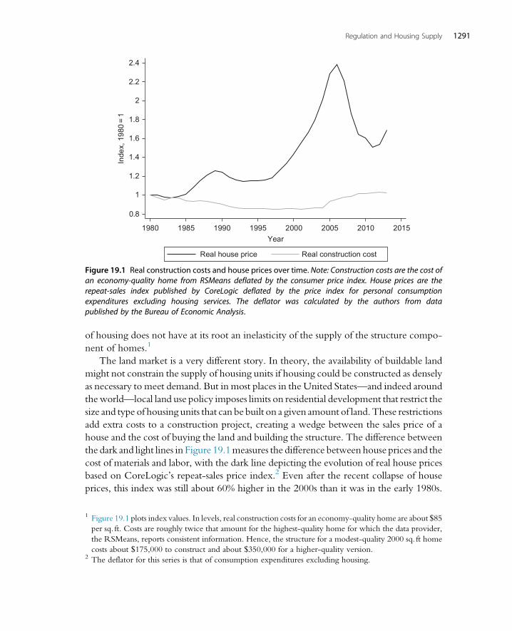
of housing does not have at its root an inelasticity of the supply of the structure compo-

nent of homes.1

The land market is a very different story. In theory, the availability of buildable land

might not constrain the supply of housing units if housing could be constructed as densely

as necessary to meet demand. But in most places in the United States—and indeed around

theworld—local land use policy imposes limits on residential development that restrict the

size and type of housing units that can be built on a given amount of land.These restrictions

add extra costs to a construction project, creating a wedge between the sales price of a

house and the cost of buying the land and building the structure. The difference between

the dark and light lines in Figure 19.1measures the difference between house prices and the

cost of materials and labor, with the dark line depicting the evolution of real house prices

based on CoreLogic’s repeat-sales price index.2 Even after the recent collapse of house

prices, this index was still about 60% higher in the 2000s than it was in the early 1980s.

0.8

1

1.2

1.4

1.6

1.8

2

2.2

2.4

Inde

x, 1

980

=1

1980 1985 1990 1995 2000 2005 2010 2015

Year

Real house price Real construction cost

Figure 19.1 Real construction costs and house prices over time. Note: Construction costs are the cost ofan economy-quality home from RSMeans deflated by the consumer price index. House prices are therepeat-sales index published by CoreLogic deflated by the price index for personal consumptionexpenditures excluding housing services. The deflator was calculated by the authors from datapublished by the Bureau of Economic Analysis.

1 Figure 19.1 plots index values. In levels, real construction costs for an economy-quality home are about $85per sq. ft. Costs are roughly twice that amount for the highest-quality home for which the data provider,

the RSMeans, reports consistent information. Hence, the structure for a modest-quality 2000 sq. ft home

costs about $175,000 to construct and about $350,000 for a higher-quality version.2 The deflator for this series is that of consumption expenditures excluding housing.

1291Regulation and Housing Supply

The growing wedge between house prices and construction costs illustrates that the price

of land has been trending upward over time. Although a portion of the increase in land

prices undoubtedly owes to geographic constraints (a topic to which we will return later),

man-made constraints alsomust play an important role.Otherwise, valuable landwould be

built out at a far-higher density than currently exists (Glaeser and Gyourko, 2003).3

Interest in how local land use regulation might have influenced the elasticity of hous-

ing supply has increased over the past few decades. This attention is at least partly due to a

suspicion that the local residential land use regulatory environment has grown stricter and

become more binding over time, particularly in areas facing strong demand for entry.

Gyourko et al. (2013) reported evidence consistent with the hypothesis that new housing

construction in local markets generally was not constrained prior to the 1970s, as during

that period, high house price growth almost always was accompanied by a large amount

of residential construction. In later decades, house price increases coincided with much

less construction, pointing to constraints on the housing supply. The idea that supply

constraints began to bite after the 1970s also is consistent with Frieden (1979), who

was among the first to argue that what we now call NIMBYism was one factor behind

the rise of environmental impact rules to slow or stop development.

Modern-day land use regulation in the United States began with zoning laws in the

1910s with the intention of separating different types of land use, thereby limiting the

negative externalities associated with certain types of industrial or commercial use

(Fischel, 2004; Quigley and Rosenthal, 2005). By and large, land use in the United States

is controlled by local governments. The US Constitution did not grant the federal gov-

ernment authority to regulate land, and the states have generally left this power with local

governments.4 The fact that land use is controlled by local governments has contributed

to the heterogeneity of regulations. Over time, the types of regulations have expanded

and now include urban growth boundaries, minimum lot sizes, density restrictions, and

height restrictions, among many others.

In this chapter, we review the research on regulation to date and highlight a number

of promising areas for future exploration. We restrict our discussion to rules and laws

imposed by any form of government that restricts the number, location, quality, or shape

of residential development. We do not discuss actions by private organizations such as

homeowners associations or regulations pertaining to commercial development because

those topics would require a much longer review.

Despite the growing body of literature on housing supply regulation, there is still

much that we do not understand. As we discuss more fully in the next section, research

on this topic has been hampered by a lack of direct evidence on regulation. The degree of

3 Not all man-made constraints are regulatory in nature. For example, Brooks and Lutz (2012) showed that

in urban Los Angeles, frictions related to assembling contiguous parcels of land restrict development.4 Some European countries like the United Kingdom and France do have national planning guidelines.


local land use restrictiveness is challenging to define because constraints can come in so

many different forms. The best information on regulation comes from surveys. Some sur-

veys collect data from a large number of jurisdictions within a single metropolitan area,

while others collect data from a few jurisdictions in a large number of metropolitan areas.

Either way, it is then up to the researcher to combine the results in order to depict most

accurately the strength of regulation. Not surprisingly, this is a difficult task because the

relative importance of different types of regulations is not well understood. A second

major empirical problem is that we do not have good time series with which to measure

changes in regulation. With only cross-sectional evidence, it is very difficult to disentan-

gle the causes and effects of regulation from local demographic and socioeconomic char-

acteristics that might be correlated with regulation. A third challenge is that many of the

predicted determinants of regulation are likely to have independent effects on housing

market outcomes even in the absence of regulation. Thus, even with the benefit of time

series data, it is challenging to identify the effects of regulation.

After discussing issues related to the measurement of regulation and reviewing a num-

ber of data collection efforts, we turn to research on the determinants of regulation.Many

theories have modeled the role of homeowners as the primary supporters of these reg-

ulations because they have a clear incentive to block development in order to protect the

value of their property. We also discuss the effect that a limited supply of vacant land,

stemming from either geographic constraints or past development, may have in encour-

aging regulation. A third important strand of the literature considers the fiscal and exclu-

sionary motives for zoning.

We then examine the consequences of regulation, the vast majority of which have

focused on effects in the housing market. The simplest models predict that regulation will

reduce the elasticity of housing supply, resulting in larger house price increases and slower

growth in the quantity of housing as demand increases. Measurement issues notwith-

standing, most papers do find a strong positive relationship between regulation and house

prices and a strong negative relationship between regulation and construction. Regula-

tion also appears to reduce the responsiveness of the housing supply to demand shocks, as

well as influence the size of metropolitan areas and the type of structures that are built.

There has been much less research examining the effects of regulation beyond housing

markets. A few papers have found that regulation is associated with household sorting

by income or other demographic characteristics, while others have found that regulation

reduces the elasticity of labor supply by altering the migration patterns of workers.

The penultimate section reviews work on the welfare consequences of local land use

regulation. Government intervention can have both costs and benefits, so one cannot

presume that regulation in this area is inefficient per se. Some regulations such as building

codes banning asbestos in insulation materials or requiring fire-retardant roofing products

almost certainly have benefits that exceed their costs, and consequently, they seem

favored by most of society. More general zoning regulations are challenging to evaluate.


For example, Hamilton (1978) showed conceptually that zoning could help local juris-

dictions provide efficient levels of public services and allow homebuilders to sort so that

housing consumption was efficient, too. However, Barseghyan and Coate (2013)

recently showed that this conclusion does not hold in a dynamic context in which exist-

ing structures are exempted from any new zoning regulation. In that case, it is possible for

there to be “overzoning” in which housing consumption is inefficiently high (although

public service provision need not be). Much remains to be done on this important topic,

but recent empirically oriented research suggests that the overall efficiency losses from

binding constraints on residential development could be quite large (Glaeser et al.,

2005; Turner et al., 2014). In the final section of this chapter, we discuss some areas where

more research would be particularly beneficial.

19.2. DATA: OLD AND NEW

Data collection and measurement have lagged behind theory and modeling from the

beginning. Perhaps, the most important reason is that development can be affected in

a myriad of ways. The heterogeneity of regulations is well illustrated by one of the earliest

surveys of land use regulation, a survey of hundreds of communities in California by

Glickfeld and Levine (1992) that collected information on 14 different controls and reg-

ulations and two catch-all “other” categories. They found that interventions were wide-

ranging in nature and included infrastructure requirements (which are called exactions in

some more recent surveys), height restrictions, caps on the number of housing units built

or permitted, population growth limits, urban boundaries or green zones, restrictions on

rezoning for a less intense land use, restrictions on upzoning to a more intense land use

(including requiring voter approval), and supermajority rules for a zoning board or city

council to approve zoning requests.5 Subsequent researchers have asked about additional

regulations such as minimum lot size requirements, as well as delays in local government

decision-making (often called “approval lags”).

There is no agreement among scholars or practitioners upon a single definition of the

degree by which development in a local land market is constrained. Nor is there a con-

sensus that one particular regulation or subset of constraints is most important. In the

absence of a common understanding, it should not be surprising that empirical work

has focused on aggregate measures of regulation, often indexes of individual rules. If com-

munities use different types of regulation as substitutes, then measuring only one type

could provide a misleading picture of the locations where regulation is generally stricter.

But it is difficult to collect accurate data on the wide variety of regulations in place, not to

mention to compare the stringency of one type of regulation with another.

5 The typical jurisdiction in theGlickfeld andLevine (1992) survey had at least twoof the above interventions.

All types of regulation existed in multiple jurisdictions. See table 2 of their paper for more details.


19.2.1 Indirect measurementOne way to bypass the difficulty of accurately measuring complex local land use envi-

ronments is to impute the presence of binding restrictions using simple economic anal-

ysis. Regardless of whether binding local constraints on housing supply exist, standard

neoclassical theory implies that price equals average cost as long as the market is suffi-

ciently competitive. Glaeser et al. (2005) argued that a large gap between prices and mar-

ginal construction costs is a clear signal that a market is tightly regulated. It is worth noting

that the housing supply can be slow to adjust to changes in demand, so prices can deviate

from costs in the short run even in an unregulated market. Thus, the fact that the dramatic

rise and fall of house prices in the late 2000s does not appear to be correlated with observ-

able measures of regulation, as observed by Davidoff (2013), does not conflict with the

idea that persistent deviations of prices from costs reflects regulation.

Glaeser et al. (2005) applied their argument to the market for Manhattan condomin-

iums, where in the absence of regulation, building heights should rise to the point where

themarginal cost of adding an extra floor equals average cost. Regardless of restrictions on

building size, free entry of builders still should keep price equal to average cost. Assuming

that the marginal cost function is increasing, as seems plausible because it is more chal-

lenging to build up, regulation implies that both prices and average costs will be above

marginal costs. Consequently, Glaeser et al. (2005) used the difference between market

price and the marginal cost of building an additional floor to proxy for the extent of hous-

ing supply restrictions.6 They labeled this gap a “regulatory tax” and concluded that it

caused Manhattan condominium prices in the beginning of the 2000s to be at least

50% higher than would the case under a completely free development policy.

Glaeser and Gyourko (2003) and Glaeser et al. (2005) performed a similar analysis for

single-family housing markets across the nation. While the underlying economic logic is

the same, empirical implementation is more difficult for this sector because one needs to

know the free market price of land in order to determine the marginal cost of supplying

an extra home. Unfortunately, there are relatively few observations on sales of vacant

land, especially in densely occupied areas.7 Various statistical techniques involving

hedonics can be used, but estimation error of the regulatory tax is likely to be larger

in the single-family sector than in a market dominated by high rises.8 That caveat aside,

Glaeser et al. (2005) reported a wide range of “regulatory tax” estimates for single-family

6 Consulting engineers can provide fairly precise estimates of this cost because additional land is not needed

to build up.7 Recently, some researchers have used data on land sales collected by the CoStar Group, Inc. See, for exam-

ple, Turner et al. (2014) and Nichols et al. (2013).8 The recent house price cycle provides a helpful illustration of how incorporating land prices matters for

calculating the regulatory tax. Davidoff (2013) showed that the magnitude of the recent boom and bust in

house prices across metropolitan areas is uncorrelated with the degree of regulation. However, one should

not conclude that the regulatory tax is uncorrelated with regulation because land prices rose and fell sharply

in the same areas where the house price cycle was most pronounced (Nichols et al., 2013).


markets across the country as of 1999–2000, ranging from zero in Birmingham, Cincin-

nati, and Houston to nearly 20% of total house value in Boston, over 30% in Los Angeles,

and upward of 50% in the San Francisco Bay Area.

Not only does one not need detailed information on the local regulatory environment

with this approach, but also it provides a natural way to summarize the strength of reg-

ulations across a heterogeneous set of laws that affect land use. The downside, of course, is

that the evidence is indirect, so it cannot provide insight into the impact of any specific

policy. Moreover, for most housing markets, it requires an assessment of the marginal

price of vacant land, which is not easy to measure. Given the difficulty in measuring land

prices and the dependence of this approach on certain assumptions, it seems wise to con-

clude that local regulatory restrictions are binding and economically important only

when the estimated “regulatory tax” is large.9 Even so, the available research suggests this

tax is quite large for many markets, which indicates that it is worthwhile for researchers to

invest in examining specific regulations in different locations across the nation.

19.2.2 Building codesAmong the first empirical efforts to collect data on housing supply regulation were those

that looked into the role of building codes, which are regulations with the stated purpose

of assuring the safety and sanitation of homes and limiting the negative externalities asso-

ciated with low-quality construction. These regulations tend to raise the cost of construc-

tion by restricting the types of materials used or the method of construction, but they do

not directly limit the quantity of housing that can be built on any given amount of land.

Noam (1983) is an early example of research on this topic, which used data collected

by the CityManagers’ Association for 1100+ cities and towns to create an index of strict-

ness of the local building code based on 14 traits or code provisions.10 We discuss empir-

ical studies of the impact of regulation in Section 19.4, but suffice it to say that Noam

(1983) reported a statistically significant correlation between local house prices and build-

ing code strictness in a cross-sectional regression of price on a code strictness index and

other covariates. As noted in the “Introduction,” the higher price well may be worth the

cost, so no welfare conclusions can be drawn from this correlation. Moreover, as we will

discuss in Sections 19.3 and 19.4, building codes may be more common in high-priced

areas so the simple correlation between regulation and house prices likely overstates the

true causal effect.

9 Housing is heterogeneous in nature, so small differences between prices and costs could reflect measure-

ment error in either variable. See Glaeser et al. (2006a) for a discussion of other relevant assumptions, the

most important being a competitive supply of homebuilders.10 See Colwell and Kau (1982) and Oster and Quigley (1977) for other early analyses using data on building

codes.


While building codes appear to be correlated with housing prices, they likely raise the

price of the housing structure rather than the land that the housing unit occupies. As we

showed above, it appears to be land prices that are the root of high and rising house prices

in the United States. This conclusion is confirmed by other research showing that land

prices have been rising for the nation in aggregate for some time, in contrast to real con-

struction costs (e.g., Davis and Heathcote, 2004; Davis and Palumbo, 2008; Nichols

et al., 2013). As land has become a larger share of the total price of a home, it is perhaps

not surprising that a growing amount of effort has turned to measuring local land use

restrictions rather than the regulations that affect the quality of residential structures.

19.2.3 Land use controlsThe first studies of land use regulation generally involved narrowly targeted data collec-

tion efforts to analyze a specific issue. In a study of how growth controls affect house price

growth, Segal and Srinivasan (1985) asked staff members of local and regional planning

agencies across 51 metropolitan areas to estimate the percentage of land removed from

development out of otherwise developable suburban land. Katz and Rosen (1987) were

even more targeted, using information from a mail and phone survey conducted by the

Center for Real Estate andUrban Economics at the University of California–Berkeley on

growth management programs in cities and towns throughout the San Francisco Bay

Area. A community was deemed to operate under a growth management program if

it had a specific cap on the number of building permits that could be issued in any given

year between 1973 and 1979. A simple OLS regression of local house prices on a dichot-

omous indicator for the presence of a growth management program found that prices

were 17% and 38% higher in communities with such programs.11 Of course, as we will

discuss below, this cross-sectional correlation probably gives a biased estimate of the effect

of regulation because communities with growth management programs are different

from other communities in many ways that likely affect house prices.

Such an economically large relationship piqued interest in the role of local land use

constraints and helped stimulate the development of broader indexes of regulatory

control. Among those that followed were Linneman et al. (1990), Glickfeld and

Levine (1992), Levine (1999), Evenson and Wheaton (2003), Foster and Summers

(2005), Quigley and Rosenthal (2005), Pendall et al. (2006), Glaeser et al. (2006b),

Gyourko et al. (2008), Glaeser and Ward (2009), and Saiz (2010). Space limitations

prevent us from reviewing each data collection effort in detail. Fortunately, the range

11 Other early data collection efforts include a 1984 survey on economic development conducted by the

International City Management Association. This survey was sent to the chief administrative officer of

various cities and contained four questions pertaining to constraints on construction. See Clark and

Goetz (1994) for more on this survey. At the state level, the American Institute of Certified Planners con-

ducted a survey of the types of land use planning activity undertaken by each of the 50 states. Those results

were published in a 1976 book Survey of State Land Use Planning Activity.


of efforts, including their strengths and weaknesses, can be illustrated by contrasting three

recent empirical efforts: Glaeser et al. (2006b), Gyourko et al. (2008), and Saiz (2010).

The first question faced by data collectors in this area is precisely what to measure.

Perhaps, the most straightforward way is to place a numerical cap on new quantity—

the type of restriction cataloged and studied by Katz and Rosen (1987). But the supply

of housing can be limited inmany other ways includingminimum lot sizes, height restric-

tions, setback requirements, and open-space designations. Regulations that affect the cost

of construction can also influence the supply of housing, as indicated by Noam’s (1983)

analysis of local building codes. Even these examples do not come close to capturing the

range of efforts devised by communities to influence housing supply. Creativity on the

part of local governments appears to know virtually no bounds in this instance.

Heterogeneity in land use restrictions across localities is so extensive that it is almost

impossible to describe the full complexity of the local regulatory environment. One strat-

egy is to focus on a small set of locations and collect as much detailed data as possible on all

aspects of the regulatory environment in those places. Glaeser, Schuetz, andWard (GSW,

hereafter; 2006b) did so for a subset of the Boston metropolitan area. Their detailed anal-

ysis of local zoning provisions allowed them to compute fairly precise estimates of the

potential housing supply in all localities in their sample. However, the enormity of that

effort prevents it from being easily replicated in many other markets.

Whereas GSW (2006b) reflected a “deep but narrow” approach to studying regula-

tion, an alternative strategy is to go “shallow but wide.” A good example of this latter

approach is Gyourko, Saiz, and Summers (GSS, hereafter; 2008), who estimated indexes

of the stringency of the local land use environment for 2611 communities across the

nation, of which approximately three-quarters are in 293 distinct metropolitan areas

spread across all 50 states. They achieved this breadth of coverage at the cost of detailed

knowledge of the environment.

GSS (2008) constructed their regulatory index based on the answers to three sets of

questions. The first inquired about the general characteristics of the regulatory process:

Who is involved in that process (e.g., states, localities, councils, legislatures, and courts)

and who can approve or veto zoning or rezoning requests. A second set of questions per-

tained to the local rules: Were there binding limits on quantities supplied? Minimum lot

size requirements? Affordable housing requirements? Development exactions of various

types? The final set of survey questions asked about changes in the cost of lot develop-

ment and in the review time for a typical project over the previous 10 years.12

12 GSS (2008) supplemented their survey responses with data from two other sources. One was the state-

level analysis of the nature of legal, legislative, and executive actions pertaining to land use policy that was

conducted by Foster and Summers (2005). The other was a measure of community pressure using infor-

mation on environmental and open-space ballot initiatives. The interested reader should see GSS (2008)

for more on these data.


The answers to these questions were used to create an aggregate measure of the strin-

gency of the local land use regime that GSS called the Wharton Residential Land Use

Regulation Index (WRLURI). Specifically, they used factor analysis to create this sum-

mary metric from 11 subindexes that described different aspects of the local regulatory

environment, with the results standardized to have a sample mean of zero and a standard

deviation of one.13 The index is increasing in the restrictiveness of regulation. Table 19.1

reproduces table 11 from GSS (2008) that reports average WRLURI values for the

47 metropolitan areas in their sample that had more than 10 communities responding

to the survey.

The index itself is constructed so as to rank places in terms of the degree of strictness

of the local residential land use environment, but the underlying survey data allow us

to describe an average community, as well as strongly and weakly regulated ones. The

typical community in theWRLURI sample can be characterized as follows: (1) two enti-

ties (zoning commission, city council, environmental review board, etc.) must approve

any project requiring a zoning change; thus, multiple points of approval now are required

for projects that cannot be done “by right”14; (2) there is a modest minimum lot size

requirement, but for the typical community, it is far less onerous than the 1 acre mini-

mums seen in highly regulated places; (3) some type of development exaction program

exists15; and (4) there is about a 6-month lag between the submission of a permit for a

standard project (where standard is defined by the community filling out the survey) and

the issuance of that permit.

Dividing the WRLURI communities into thirds and labeling the top third “highly

regulated” and the bottom third “lightly regulated” allows us to contrast traits across those

two groups. One noteworthy distinction is that local and state pressure groups are much

more likely to be involved in the regulatory process in the more highly regulated places.

Another key distinguishing feature between highly and lightly regulated communities is

that more than 50% of the highly regulated communities have a 1 acre minimum lot size

rule in at least one neighborhood, whereas less than 5% of lightly regulated communities

have such a rule. Open-space requirements and some type of formal development exac-

tions policy are nearly omnipresent in the highly regulated localities, but often are not

present in the most lightly regulated areas. In addition, the average delay time between

13 More specifically, the principal component of each subindex was used to create the community-wide

index. The 11 subindexes include a local political pressure index, state political involvement index, state

court involvement index, local zoning approval index, local project approval index, local assembly index,

supply restrictions index, density restrictions index, open-space index, exactions index, and approval delay

index. The literature has not reflected on how to aggregate across individual regulations, but it certainly

would be beneficial to consider what an optimal weighting scheme might look like.14 A project can be done “by right” if it meets all published zoning regulations and requires no variances of

any kind.15 Development exactions are monetary or in-kind payments in return for development rights.


Table 19.1 Average WRLURI values for metropolitan areas with data on 10 or more local jurisdictions

Metropolitan area WRLURINumber ofobservations Metropolitan area WRLURI

Number ofobservations

1. Providence–Fall River–Warwick, RI–MA 1.79 16 25. Milwaukee–Waukesha, WI 0.25 21

2. Boston, MA–NH 1.54 41 26. Akron, OH 0.15 11

3. Monmouth–Ocean, NJ 1.21 15 27. Detroit, MI 0.12 46

4. Philadelphia, PA 1.03 55 28. Allentown–Bethlehem–Easton, PA 0.10 14

5. Seattle–Bellevue–Everett, WA 1.01 21 29. Chicago, IL 0.06 95

6. San Francisco, CA 0.90 13 30. Pittsburgh, PA 0.06 44

7. Denver, CO 0.85 13 31. Atlanta, GA 0.04 26

8. Nassau–Suffolk, NY 0.80 14 32. Scranton–Wilkes–Barre–Hazelton, PA 0.03 11

9. Bergen–Passaic, NJ 0.71 21 33. Salt Lake City–Ogden, UT �0.10 19

10. Fort Lauderdale, FL 0.70 16 34. Grand Rapids–Muskegon–Holland, MI �0.15 16

11. Phoenix–Mesa, AZ 0.70 18 35. Cleveland–Lorain–Elyria, OH �0.16 31

12. New York, NY 0.63 19 36. Rochester, NY �0.17 12

13. Riverside–San Bernardino, CA 0.61 20 37. Tampa–St. Petersburg–Clearwater, FL �0.17 12

14. Newark, NJ 0.60 25 38. Houston, TX �0.19 13

15. Springfield, MA 0.58 13 39. San Antonio, TX �0.24 12

16. Harrisburg–Lebanon–Carlisle, PA 0.55 15 40. Fort Worth–Arlington, TX �0.27 15

17. Oakland, CA 0.52 12 41. Dallas, TX �0.35 31

18. Los Angeles–Long Beach, CA 0.51 32 42. Oklahoma City, OK �0.41 12

19. Hartford, CT 0.50 28 43. Dayton–Springfield, OH �0.50 17

20. San Diego, CA 0.48 11 44. Cincinnati, OH–KY–IN �0.56 27

21. Orange County, CA 0.39 14 45. St. Louis, MO–IL �0.72 27

22. Minneapolis–St. Paul, MN–WI 0.34 48 46. Indianapolis, IN �0.76 12

23. Washington, DC–MD–VA–WV 0.33 12 47. Kansas City, MO–KS �0.80 29

24. Portland–Vancouver, OR–WA 0.29 20

Notes: This table appears as table 11 in Gyourko et al. (2008). Metropolitan area definitions are based on the 1999 boundaries. Consolidated metropolitan statistical areas are disaggregated intoprimary metropolitan statistical areas wherever relevant.

application and approval for a standard project in the highly regulated communities is

three times longer than in the lightly regulated communities (10.2 months vs. 3.2

months, respectively).

Another noteworthy feature of theWRLURI is the strong positive correlation across

its component indexes. Essentially, if a community is rated as highly regulated on one

dimension, it is likely to be highly regulated along other dimensions. This result suggests

that surveys covering only a limited set of types of regulation might provide a reasonably

accurate picture of the general restrictiveness of the locations in the sample, but further

research should examine this conjecture more thoroughly.

In terms of data detail and market coverage, the contrast of GSS (2008) with GSW

(2006b) is stark. Whereas GSS (2008) only know whether a town had a 1 acre minimum

lot size restriction in at least one neighborhood, GSW (2006b) know how every square

yard in the entire municipality is zoned. For example, there are 14 municipalities in the

GSWsamplewithminimum lot sizes in excess of 70,000 sq. ft (over 1.6 acres). Those areas

constitute more than 10% of the region’s land area but hold only 4% of the population.

More generally, the diversity of minimum lot size restrictions in the Boston area is stag-

gering, with the range running from less than 10,000 sq. ft to more than 70,000 sq. ft. The

modal minimum lot size restriction is roughly 1 acre, providing some indication of how

stringent the zoning codes are in many of the communities in the GSW sample.

The detailed knowledge of the local regulatory environment amassed by GSW

(2006b) was collected over a 2-year period in which the authors worked with a team

of researchers at the Pioneer Institute for Public Policy Research to catalog the land

use regulatory environment in 187 communities that comprise a subset of the Boston

metropolitan area. They conducted a survey of over 100 questions, interviewed local

officials, and provided those individuals the opportunity to review the results. Such detail

is only possible within a given metropolitan area and could only be replicated in other

regions at high cost.

The benefits are considerable. The Boston metropolitan area is worthy of detailed

analysis because key summary statistics suggest it is very tightly regulated. In the midst

of high and rising real house prices over time, the number of housing permits has shrunk

considerably: from 172,459 in the 1960s to 141,347 in the 1980s and down to 84,105 in

the 1990s (GSW, 2006b). GSW (2006b) recognized the possibility that the reason for the

downward trend in construction could be that Boston is running out of land, rather than

man-made regulation. However, the authors showed that densities outside the urban

core are quite low, suggesting that land is still plentiful in the Boston area.16

16 Moreover, if it were land that really was scarce, the price of a quarter acre of extra land would be the same

whether it extends an existing lot or sits under a new home. Glaeser and Gyourko (2003) showed this not

to be the case for the Boston area.


This result led GSW (2006b) to a detailed study of local zoning codes. In doing so,

they provided a rare window into the intricacy of these laws. Their survey includes not

only the hard caps on growth akin to those studied by Katz and Rosen (1987) but also the

prohibition of irregularly shaped lots, extensive wetlands restrictions, septic system reg-

ulations, and various subdivision rules. Not all rules are designed to limit supply, as there

are also “cluster provisions” and inclusionary zoning provisions, which allow developers

to build at higher densities in some places, and age-restricted zoning that typically

encourages building for seniors.

GSW (2006b) used historical data on permits in their communities (going back to

1910 using decennial Census data) to investigate which of the myriad of regulations really

matter in terms of constraining residential construction. They concluded that evidence

linking minimum lot size restrictions to new development is especially persuasive.

As minimum lot size increased by a quarter acre, roughly 10% fewer houses were per-

mitted over time. This negative relationship between regulation and permits was found

even in communities with lower minimums. Relatively strict wetland regulation also

appears to constrain new development in an economically meaningful way. In a

follow-up paper (Glaeser andWard, 2009), two of these authors used these data to exam-

ine the causes and consequences of regulation in more detail. We will discuss those find-

ings below.

19.2.4 Other measuresBeyond investigating building codes or land use regulation, another method of inferring

restrictiveness of supply can be found in Saiz (2010), who incorporated the role of topog-

raphy to estimate the elasticity of housing supply for nearly 100 metropolitan areas in the

United States. His approach used three separate data sources. First, he employed GIS

techniques to compute the area lost to oceans within a 50 km radius of the centroid

of a metropolitan area. Second, he used satellite data from the US Geological Survey

(USGS) to calculate the amount of land lost to internal water bodies and wetlands. Third,

under the rationale that anything above a 15° slope is extremely challenging and expen-

sive to build on, he used the USGS Digital Elevation Model to compute the percentage

of land area with a slope in excess of 15°. Taken together, these three computations pro-

vide an estimate of exogenously undevelopable land in a metropolitan area.

Saiz (2010) then proceeded to investigate links between geography, regulation, and

urban development. As we will discuss below, he found a strong statistical link between

his estimates of geographic restrictions and theWRLURI. That is, regulatory restrictive-

ness tends to be higher in metropolitan areas that have geographic constraints on land

development in terms of being coastal, having internal water bodies of some type

and/or steep elevations. Based on the geographic constraints and WRLURI, Saiz

(2010) estimated the elasticity of housing supply for each of the metropolitan areas in


his sample. These estimates have been used by many other researchers to analyze the

housing supply and to provide exogenous variation in house prices across locations.

19.2.5 Summary of measurement issues and concluding commentsIn the past decade or so, there have been considerable achievements in the measurement

of local land use regulations. Early studies focused on only a single type of regulation

within a fairly limited geographic area. By contrast, GSW (2006b) provided a very

detailed picture of the entire regulatory environment of a single metropolitan area.While

it is very costly to amass this type of information, it would be helpful to replicate their

survey in other metropolitan areas as often as possible. Combining data from such detailed

studies of land use regulation would be even more valuable than examining a single area

in isolation.

More effort has been put into less specific andmore general measurement of local land

use regulatory environments across a wider range of communities, as reflected in the GSS

(2008) survey of more than 1900 communities in over 290 metropolitan areas. Although

this survey does not contain detailed information on all the different ways local govern-

ments can constrain residential development, the advantage is in allowing researchers to

compare regulation across many more localities and markets.

Beyond surveys, Saiz (2010) illustrated the possibility of using other data to gain

insight into the elasticity of housing supply. Using the geography and topography of

the land, he documented a connection between geographic constraints and regulatory

constraints and provided estimates of housing supply elasticities for nearly 100 metropol-

itan areas.

Because surveys are so expensive in terms of time and money, researchers should be

creative in thinking about other ways to measure regulation using readily available data.

One possibility is to use public records data, which are now routinely collected and sold

by a few data providers. These datasets, which cover the vast majority of residential prop-

erty in the United States, include parcel-by-parcel information on allowed land use. For

example, Brooks and Lutz (2014) use land use codes from public records data to analyze

zoning and public transit in Los Angeles. Another possibility might be to use data from

Internet chatter, as in Gyourko and Saiz (2006).

As will be documented below, measures of local land use restrictiveness have been

widely used in subsequent empirical research into the causes and consequences of reg-

ulation. However, they are limited in the sense that each is a cross-section. Because reg-

ulation can be correlated with many other attributes of a location, a single snapshot of the

local regulatory environment is not conducive to establishing causality in empirical work.

Thus, it is critical that researchers collect new data or otherwise come up with ways

to measure changes in regulation over time. For example, Glaeser andWard (2009) con-

verted the GSW (2006b) survey into panel data based on the year that different types of


regulation are adopted. Similarly, Jackson (2014) converts the Glickfeld and Levine

(1992) survey into a panel of regulations in California.17 Besides panel data, another

helpful approach would be to examine changes in a particular regulation using a

difference-in-difference strategy. A few examples are Zhou et al. (2008), who analyzed

the effect of an amendment to the Chicago Zoning Ordinance; Cunningham (2007),

who analyzed the adoption of an urban growth boundary in Seattle; Kahn et al.

(2010), who analyzed the creation of a coastal boundary zone in California; and

Thorson (1997), who analyzed an increase in minimum lot sizes inMcHenry County, IL.

19.3. DETERMINANTS OF REGULATION

19.3.1 Joint determination of land values and zoningOne of the earliest questions asked in the literature on the determinants of zoning is

whether local governments set zoning laws in order to maximize the value of land in their

jurisdiction. For example, Wallace (1988) modeled zoning as the outcome of a county

council that maximizes its utility, which is a function of land attributes and land prices.

Land prices are also a function of local characteristics, as well as of the zoning designation

chosen. If zoning has no effect on land values, then one would conclude that these reg-

ulations merely coincide with the land use that would be adopted in unconstrained mar-

kets. Wallace refers to this question as whether “zoning follows the market.” In a sample

of parcels for Kings County, WA, she found that zoning allocations tend to decrease the

price of parcels zoned for large lots, suggesting that zoning leads to an oversupply of large

minimum lot sizes.18 More generally, she found that land values would be higher under

different zoning designations. Thus, she concluded that in this sample, zoning does not

“follow the market.” Her analysis uses observed attributes of land parcels to correct for

the selection of different types of land into different zoning categories. However, it is

difficult to rule out the alternative interpretation that unobserved variables cause cheaper

land to be zoned for larger lots.

McMillen and McDonald (1991) also estimated a model in which land values affect

zoning decisions, and vice versa. In their data from the northwest suburbs of Chicago,

they identified the determinants of zoning from an indicator of whether a parcel was

located in Cook County, because that county was more likely to zone undeveloped land

17 Although these efforts are clearly a vast improvement over cross-sectional data, they do not account for

regulations that no longer existed at the time of the survey. Thus, if cost were not an issue, repeated surveys

would be a better method of constructing panel data than using the implementation date of existing

regulations.18 Because zoning and land values are jointly determined, she identifies a two-equation model of land values

and zoning using an indicator for whether a parcel is platted as an instrument for land values. The justi-

fication for this specification is that approval of a plat application entails considerable time and monetary

costs, raising the price of land, and that the zoning designation is decided prior to when a parcel is platted.


for residential use. They found that zoning patterns reflect characteristics of the land in

that parcels closer to railways and expressways are more likely to be designated for

manufacturing use. They also showed that estimates of the land value equation are biased

when one does not account for the endogenous designation of zoning.

In a sample of home sales in Santa Clara County, CA, Pogodzinski and Sass (1994)

differentiated between the effects of land use designations and regulations that affect the

characteristics of a lot and its structure. They found that land use designations do not

affect house values, implying that this type of zoning does “follow the market.” By con-

trast, minimum lot sizes, minimum side-yard restrictions, and maximum height restric-

tions do affect house values, implying that these types of regulations do not “follow the

market.”

To summarize, this early work has generally found that zoning regulations do not

simply mimic the outcome that would result from an unregulated market. However,

because their focus is on the effect of regulation on land values, these papers provide little

insight into the factors that do shape housing supply regulation.

19.3.2 Homeowners, developers, and local politics in a single communityMore recent theories concerning the determinants of regulation have incorporated the

idea that local residents do not all share the same goals, so the regulatory environment will

be shaped by the incentives and influence of actors in the local political process. In a num-

ber of influential articles and books, William Fischel has advanced the idea that home-

owners are an important force behind these types of regulation.19 In The Homevoter

Hypothesis (2001), he contended that homeowners have a strong incentive to work

together in order to restrict undesired development because their home is typically their

primary asset and owners do not have other means to insure against events that would

reduce their property value. Central to Fischel’s argument is the idea that local amenities

and disamenities (such as school quality and dumps) are capitalized into house values. In

support of this notion, he cited a number of studies finding that house prices are lower in

neighborhoods with disamenities such as a toxic waste dump, more through traffic, or

more localized air pollution, as well as research showing that property tax rates are cap-

italized in house prices. Because shocks to housing wealth are difficult to insure or diver-

sify, homeowners turn to local political action to protect their investment.

According to Fischel, another reason why homeowners are so opposed to develop-

ment is that they tend to work in a different jurisdiction than where they live. When

construction is pushed into a nearby jurisdiction, homeowners can benefit from some

19 Fischel drew on earlier work discussing the role of homeowners in constraining local development includ-

ing Sonstelie and Portney (1978) and Ellickson (1977). In an early book, Fischel proposed that local gov-

ernments impose land use regulation in order to maximize the value of owner-occupied housing (Fischel,

1985).


positive effects, such as job creation, without incurring the cost of higher density in their

own neighborhood. This logic can explain both why regions with more fragmented gov-

ernments are more likely to have stricter regulation (Fischel, 2008) and why regulation

spread and became stricter over the twentieth century along with suburbanization

(Fischel, 2004).

Drawing on Fischel’s insights, a number of papers have developed more formal the-

oretical models of homeowners’ influence on zoning regulation. Ortalo-Magne and Prat

(2014) present a cutting-edge example, in which they used an overlapping-generations’

economy to model three decisions simultaneously: the location choice of households

(a regulated city versus unregulated countryside), investment in residential real estate,

and the collective choice model of local housing supply regulation.

Their basic setup is as follows. Households decide whether to live in the countryside,

where they pay a fixed rent and earn income normalized to zero, or in a city where

income is a function of citywide productivity that varies over time and a fixed idiosyn-

cratic component. In the city, households choose whether to invest in owner-occupied

housing or to rent. There is a fixed premium between the return to investing in owner-

occupied housing and the return to investing in rental housing, which is meant to reflect a

number of factors including the nonpecuniary benefits of homeownership and its favor-

able tax treatment, the costs of managing rental property, and moral hazard in the rental

market. Housing wealth is consumed at the end of an individual’s life. Thus, tenure

choice is a trade-off between the homeownership premium and the price risk associated

with homeownership.20 New construction in the city requires a building permit, and the

number of building permits allowed is decided by city residents through majority voting.

Permits are assigned to developers, who do not vote and who must pay a fee for every

new permit. Aggregate permit fees paid are split equally among all city residents. These

fees can be interpreted as a rough proxy for the general economic gains that development

can bring to an area.

Not only do city residents receive a share of the total permit fees raised, but also they

benefit from new construction because the larger housing supply reduces future rents and

all city residents must pay rent either to themselves or to absentee landlords. However,

the reduction in rents also causes house prices to fall, leading to lower end-of-period con-

sumption. In the model, construction does not occur if the net benefit accruing to the

median voter is negative—i.e., if the benefit owing to lower future rents and the voter’s

share of permit fees is less than the decrease in final consumption through lower house

prices.

Using this model, Ortalo-Magne and Prat showed that a homeownership subsidy

makes homes less affordable. Absent the constraints on new construction, the subsidy

20 Since households are risk-averse, without the homeownership premium, everyone would choose to rent.

Housing not owned by households is owned by risk-neutral firms.


would have no effect on affordability because it would be exactly offset by an increase in

house prices. However, the subsidy causes themedian city resident to ownmore housing,

thereby leading to more opposition to city growth. It is therefore the reduction in per-

mitted new construction that raises equilibrium house prices and reduces affordability.

In contrast to the homeownership subsidy, an increase in the permit fee boosts sup-

port for urban growth, leading to an increase in city size. The expansion of the housing

supply reduces rents, making all city residents better off. This result illustrates Fischel’s

argument that the more homeowners internalize the benefit from new construction,

the less opposed to development they will be.

Theories in the vein of Fischel and Ortalo-Magne and Prat predict that homeowners

should be stronger supporters of housing supply regulation than renters; other examples

include Glaeser et al. (2006b) and Hilber and Robert-Nicoud (2013). A few studies have

found support for this hypothesis in voting patterns. For example, Dubin et al. (1992)

documented that precincts with a larger share of homeowners had a larger proportion

of votes cast in favor of growth controls in a 1988 San Diego election. McDonald

(1995) also examined voting patterns—in this case, a proposed zoning ordinance in

Houston—and found that middle-income precincts were more likely to support a pro-

posed zoning ordinance than lower-income precincts. Although he does not examine

homeownership directly, it is likely that middle-income precincts have higher homeow-

nership rates than lower-income precincts. An interesting aspect of McDonald’s study is

that zoning did not exist in Houston, so the voting patterns do not reflect any preexisting

pattern of regulation.

If homeowners favor tighter regulation, then policy should be more restrictive in

areas where the political influence of homeowners is stronger. However, evidence for

this relationship is difficult to find. Logan and Zhou (1990) found little correlation

between homeownership and a variety of growth control measures in a national sample

of suburban municipalities in 1973. Similar results have been found for growth control

measures in cities around San Jose (Baldassare and Protash, 1982) and for municipalities in

California (Donovan and Neiman, 1995; Brueckner, 1998). It is possible that the mere

presence of homeowners is not a particularly accurate measure of the influence that these

constituents have on local policy. Instead, their influence might be better reflected by

demographic or socioeconomic characteristics of the local population that are correlated

with their ability to organize or otherwise participate in local policymaking.Many studies

have found positive correlations of regulation with socioeconomic characteristics that are

likely to be correlated with the political influence of homeowners, such as income, edu-

cation, and the fraction of white-collar or professional workers.21 However, it should be

noted that because all of these studies are cross-sectional in nature, it is difficult to rule out

21 See Lenon et al. (1996), McDonald and McMillen (2004), Evenson and Wheaton (2003), Donovan and

Neiman (1995), and Baldassare and Protash (1982). Glickfeld and Levine (1992) is an exception.


the possibility that the correlations (or lack thereof ) are driven by omitted variables.

Moreover, the model proposed by Ortalo-Magne and Prat demonstrates that because

regulation raises house prices, the degree of regulation could influence the incentive

to be a homeowner, and this reverse causality could further obscure these cross-sectional

relationships.

Relatively few papers have attempted to account for potential endogeneity problems

when examining the role of homeowners in restricting the housing supply. Hilber and

Robert-Nicoud (2013) instrumented for homeownership with the fraction of house-

holds that are married couples with no children. The idea is that married couples will

have higher and more stable incomes than single adults or households with children,

making themmore likely to qualify for a mortgage. Also, married couples are more likely

to be in stable relationships compared with unmarried couples, implying a lower prob-

ability of moving and therefore a longer period over which to recoup the transaction costs

of purchasing a home. The use of this instrument requires the assumption that the fraction

of households that are married couples with no children does not affect regulation

through any channel except the homeownership rate. In a sample of 93 metropolitan

areas in 1990, they found that locations with a larger share of married households with

no children had a higher homeownership rate in the same year. Using this instrument,

they found a positive, but insignificant, correlation with the WRLURI described in the

previous section. Moreover, the estimated effect is not large, as a one standard deviation

increase in aMSA’s homeownership rate is associated with a one-third standard deviation

increase in regulatory constraints. Of course, one still might be concerned that the frac-

tion of households that are married and without children is either influenced by housing

supply regulation or correlated with omitted variables that are also correlated with

regulation.

Glaeser and Ward (2009) used a different method to get around the endogeneity of

homeownership and regulation, examining relatively recent patterns of housing supply

regulation as a function of homeownership rates in 1940 or 1970. This method avoids the

problem of reverse causality, but it is less clear that it mitigates concerns about omitted

variables, since historical homeownership rates could also be correlated with many unob-

served attributes that affect regulation. In their sample of townships in the Greater Boston

area, the authors find little correlation of historical homeownership with a number of

measures of regulation such as minimum lot sizes, wetland bylaws, septic rules, and cluster

zoning. They also found little correlation of regulation with other 1970 attributes of

townships that might be correlated with homeowner influence, such as educational

attainment and the fraction of the population that is foreign born.

In summary, there is little empirical evidence that areas with more homeowners adopt

stricter housing supply regulations, a fairly surprising result given the many theories that

point to homeowners as the drivers of regulation. Because much of this evidence is cross-

sectional in nature, more work is needed to address the issues of omitted variables and


reverse causality. Panel data would add a useful dimension, allowing researchers to

observe how regulation changes after homeownership patterns change. As noted above,

except in a very few cases, panel data do not yet exist. Hence, it is vital to explore other

instruments for homeownership. One possibility could arise from regulatory changes in

mortgage markets that have changed the ease of getting a mortgage in a way that has had

differential effects on homeownership across locations, but would otherwise be uncor-

related with factors that affect land use policy. There are multiple conditional clauses in

that sentence, so it is by no means certain that such an instrument would be found to be

powerful and valid. However, it is critical for empirical researchers to think more cre-

atively along these lines if the causal effect of homeownership on regulation is ever to

be uncovered.

Besides homeowners, developers and/or owners of vacant land may also be important

participants in the local political process. Molotch (1976) coined the phrase “growth

machine” in reference to the idea that landowners in a community will band together

in support of policies that will fuel local economic growth. He argued that the people

who end up in local government tend to be local business leaders and other types that

are naturally sympathetic towards local growth. Thus, local policy can end up favoring

policies that promote economic activity, even if the typical citizen does not. One possible

explanation for the lack of cross-sectional correlation between homeownership and reg-

ulation is that areas with higher homeownership rates may also have stronger alliances

favoring progrowth policies, perhaps because the population is wealthier. Fischel

(2008) argued that developers have more influence in large governments, causing met-

ropolitan areas with more political fragmentation to have stricter regulation.

Few formal models have explicitly allowed for the role of developers in shaping hous-

ing supply regulation. Hilber and Robert-Nicoud (2013) and Glaeser et al. (2005)

showed how local planning boards can be influenced by both homeowners and devel-

opers. LikeOrtalo-Magne and Prat, these models predict that locations with a larger share

of homeowners will have stricter housing supply regulation. In addition, they illustrated

that regulations will be tighter in jurisdictions where homeowners have a stronger polit-

ical influence relative to developers. However, the way in which they model this influ-

ence is fairly simple. In Glaeser et al. (2005), homeowners use time to influence the local

planning board whereas developers use cash, with the result that regulation will be tighter

in areas where the planning board is more influenced by time. In Hilber and Robert-

Nicoud (2013), owners of developed land (homeowners) and owners of undeveloped

land (developers) both use cash to influence the planning board, and their lobbying con-

tributions are a positive function of the value of their land.

This topic is yet another case in which theory is ahead of empirics, as we are aware of

little empirical evidence on the influence developers have in shaping housing supply reg-

ulation. One study with indirect evidence on this front is Sole-Olle and Viladecans-

Marsal (2012), who argued that developers should be less successful at influencing local


regulations when the currently elected officials have won the vote by a narrowmargin. In

that case, the elected officials will place a higher priority on following voters’ preferences

in order to be reelected. Using data on more than 2000 Spanish municipalities from 2003

to 2007, they reported evidence in support of this hypothesis.

19.3.3 Supply of buildable land and historical density patternsOne interesting aspect of the model proposed by Hilber and Robert-Nicoud (2013) is

that the incentives of homeowners and developers to influence the planning process

are a function of the value of land. Thus, anything that raises land values will affect reg-

ulation. Specifically, in their model, jurisdictions have innate differences in amenities and

households choose among jurisdictions. The greater demand to live in an area with more

valuable amenities is only partly offset by congestion costs, leading to a positive correla-

tion between amenities and development across locations. In equilibrium, locations with

more desirable amenities will have a larger share of developed land and, consequently,

more land use regulation in order to prevent further development from raising conges-

tion disamenities even more. Consequently, a restricted supply of land (higher share of

developed land) causes further restrictions on supply in the form of government

regulation.

In support of the prediction that locations with more developed land will have more

regulation, Hilbert and Robert-Nicoud showed that metropolitan areas with a larger

fraction of developed residential land area (measured using the 1992 National Land

Cover Data) have a larger degree of regulation according to the WRLURI. This corre-

lation exists even after controlling for the homeownership rate, so it does not simply

reflect the fact that homeowners have a greater influence on local policy in areas where

they are more numerous. Further, Hilber and Robert-Nicoud instrumented for the share

of developed land with two variables reflecting natural amenities—average January tem-

perature and the presence of a major coastline—and population density in 1880, which

they interpret as reflecting the innate desirability of an area at a time long before regu-

lations were in place.22 These instruments turn out to be strong predictors of the share of

developed land in 1992, and using them, the predicted share of developed land has a pos-

itive and significant effect on regulation. Thus, they interpreted the positive correlation

22 More specifically, their argument is that natural amenities are not directly correlated with supply restric-

tions because the types of regulations that they examine do not include efforts to protect coasts and because

warm temperatures are unlikely to be significantly related to the type of environmental considerations that

typically induce planning. Saiz (2010) did, in fact, document a strong relationship between geographic

constraints, which tend to be in coastal areas, and regulation. He interpreted this relationship as causal.

However, this result does not undermine the validity of amenities as instruments for the share of devel-

opable land as long as the reason why coastal areas have tighter regulation is because they have less devel-

opable land.


between regulation and developed land as reflecting the stronger demand to regulate in

high-amenity places.23

As discussed above, Saiz (2010) followed a different empirical strategy using geo-

graphic features of the landscape to measure the supply of buildable land and hence

the restrictiveness of housing supply regulation. Saiz (2010) found that metropolitan areas

with a larger fraction of land lost to geographic constraints tend to have stricter housing

supply regulations as measured by the WRLURI. Citing the models discussed above, he

then argued that homeowners have a stronger incentive to protect their housing invest-

ment (through regulation) where land values are high initially and that geographic con-

straints lead to important initial differences in land values. In keeping with this

interpretation, Saiz (2010) found that the relationship between geographic constraints

and regulatory constraints does not hold in areas suffering from weak long-term demand

(defined as the bottom quartile of urban growth between 1940 and 1970). His proposed

explanation is that geographic constraints are not likely to bind in low-demand places

and, therefore, they are not likely to affect the incentive to regulate.

In contrast to the results documented by Saiz (2010) and Hilber and Robert-Nicoud

(2013), a few other papers have found the opposite correlation of historical density pat-

terns with regulation. In their analysis of townships in the Greater Boston area, Glaeser

andWard (2009) showed that higher housing density in 1940 and 1915 is associated with

less restrictive residential zoning in the late 1990s/early 2000s, as measured by minimum

lot size requirements. This relationship is quite strong in that density in 1940 can explain

68% of the variation in current minimum lot sizes. Going back even further, these authors

showed that towns with larger minimum lot sizes had a larger fraction of forested area in

1885. Their interpretation is that historical patterns of deforestation reflect agricultural

productivity. Locations with more productive land were developed first and had higher

land values, resulting in higher density for many years to come and eventually to regu-

lations that allowed for higher residential density.

Evenson and Wheaton (2003) also used data from Massachusetts to explore the con-

nection between land use regulation and past development patterns. They measured

actual land use in 1999 from aerial photographs taken of each town by the Massachusetts

Office of Geographic and Environmental Information and obtained parcel-level infor-

mation on zoning bylaws and the amount of land protected from development from

the same institution. The data on open land are combined with minimum lot sizes

and floor-to-area ratios to determine the maximum possible number of new buildings

23 The economic magnitude of this effect is a matter of opinion. It seems large in that assigning San

Francisco’s attributes to Salt Lake City would move the latter from the 56th most regulated area (out

of 93) to the 35th most regulated. On the other hand, a one standard deviation change in the share of

developed land is associated with only one-third standard deviation stricter regulation, which is about

the same magnitude that the authors found for homeownership, as described above.


in each town under current zoning regulation. They found that towns with relatively

high housing density in 1999 tend to zone for higher future housing densities. In addi-

tion, towns with a larger fraction of developed land devoted to residential use tend to

zone a larger fraction of open land for residential use. Like Glaeser andWard (2009), they

found that zoning regulations follow past land use patterns. They also showed that for all

but a handful of towns very close to Boston, future residential building is restricted to a

lower density than the current density (i.e., the slope of the regression line of zoned den-

sity on current density is positive but less than one). This result fits Fischel’s ideas that

residents of suburban jurisdictions are more likely to focus on the negative aspects of

allowing new construction, while residents of urban jurisdictions where many businesses

are located are more sensitive to the potential benefits of additional development.

The contrasting findings of Hilber andRobert-Nicoud and Saiz on the one hand with

those of Glaeser and Ward and Evenson and Wheaton on the other suggest that much

more work is needed to understand the connection between density patterns and regula-

tion. One difference between these two sets of results is that they use very different data.

The first two studies measure regulation using theWRLURI, which covers many aspects

of the regulatory process including the actors in the development process, statutory limits

on residential construction, and delays in permit approval, whereas the latter two studies

focus onminimum lot size zoning.24 Another important difference between these two sets

of studies is that the first examines patterns across metropolitan areas, while the second

examines patterns across jurisdictions within a single state or metropolitan area. As we dis-

cuss below, the incentives for regulating new development could be different in these two

settings. In addition to further empirical analysis examining the relationship between the

supply of buildable land and regulation, it would be helpful to consider other models that

might help explain why zoning patterns seem to be correlated with past development.25

19.3.4 Regulation in a multicommunity setting: Sorting and strategicinteractionsThus far, we have mostly focused on land use decisions in the context of a single com-

munity in isolation.26 But what happens when the population moves freely across a set of

local jurisdictions, each with the ability to set its own land use policy? A number of papers

have investigated the use of zoning to induce sorting of households across jurisdictions.

24 It could be that communities set lot sizes in a way that allows new construction to follow the density of

existing buildings but restrict new development in other ways to compensate.25 One step in this direction is Evenson and Wheaton (2002, unpublished working paper), who predict an

inverse correlation between existing residential density and restrictions on future development. The intu-

ition is that for a given population size, higher existing density implies lower aggregate consumption of

land. When existing residents consume less land, the capital gains from open-space creation become smal-

ler relative to the cost of purchasing that space, so they will set aside less open land for public use.26 The primary exception is the discussion of Hilber and Robert-Nicoud (2013), whose model incorporates

mobility across jurisdictions.


One suchmotive that has been discussed frequently in the literature is the “fiscal” motive,

which refers to a desire to limit the fiscal externality that arises when households pay tax

proportional to their income but share the benefits of public expenditures equally

(Hamilton, 1978). In that case, zoning restrictions such as minimum lot sizes allow house-

holds to sort themselves into communities with other households that have similar pref-

erences for the provision of a public good. Epple et al. (1988) developed a model where

uncertainty about the type of household that will arrive in a metropolitan area can cause

homeowners in a community to enact zoning in order to maximize the net tax contri-

bution of new entrants. Similarly, Calabrese et al. (2007) showed how homeowners will

choose to impose a lower bound on housing consumption to induce sorting across com-

munities and consequently more efficient provision of a local public good.

Rolleston (1987) argued that fiscal considerations will cause communities to compete

with one another to maintain or improve their fiscal advantage relative to other commu-

nities in their region. Therefore, zoning should be more restrictive in an area with a

“healthier” fiscal situation relative to others. In a sample of 360 communities in north-

eastern New Jersey, she created a measure of the “fiscal capacity” of a community based

on per capita income; per capita market value of residential taxable property, farm land,

and vacant land; and per capita market value of commercial, industrial, and telephone/

telegraph property. She found that relative fiscal capacity is positively related to the

restrictiveness of residential zoning, as measured by an index of minimum lot sizes for

vacant developable residential land.

Bates and Santerre (1994) also found evidence in favor of fiscal motives for zoning in a

sample of 132 municipalities in Connecticut. Specifically, they found that communities

are likely to zone a lower fraction of land for residential purposes when they have a large

nonresidential tax base, which they argued reflects a larger opportunity cost of residential

development. They also found that the fraction of vacant land zoned for residential use is

negatively related to past population growth, which they interpreted as a fiscal motivation

because rapid population growth can “impose increasing public service costs on

entrenched residents.” On the other hand, they found little correlation between these

two fiscal-motivation variables and minimum lot sizes. They also found no relationship

between the total market value of taxable property, another variable reflecting the fiscal

motive for zoning, and either measure of zoning restrictiveness.

One problem with interpreting the results found by Rolleston (1987) and Bates and

Santerre (1994) is that the variables used to measure the fiscal capacity of a jurisdiction

could also reflect a number of other factors that influence regulation. Moreover, these

measures might be affected by the amount of regulation in the area. Lutz

(forthcoming) mitigates these identification issues by examining the effect of a statewide

policy that had a differential impact on the fiscal situation of local governments. Specif-

ically, in an attempt to equalize funding for education, a reform inNewHampshire began

granting payments to towns on the basis of their property wealth. He shows that towns

with a larger grant were more likely to impose growth management regulations,


consistent with the idea that a stronger fiscal situation will cause a community to use reg-

ulation to restrict new entry.27

Another motivation for zoning that is frequently discussed in the literature is that

households may use zoning to prevent minorities and/or poor households from moving

in for reasons other than fiscal motives. This often is referred to as an “exclusionary”

motive for zoning in the literature.28 Because minorities tend to have lower incomes,

minimum lot size requirements or regulations imposing a floor on the quality of homes

can restrict access to potential minority residents and potential low-income residents. In a

sample of tracts in Santa Clara County, CA, Pogodzinski and Sass (1994) found that min-

imum lot sizes are larger in tracts with higher median incomes, which could be due to

either a fiscal or an exclusionary motive. On the other hand, it could also be due to the

fact that rich households are more adept at influencing land use policy.

Rolleston (1987) looked for evidence of exclusionarymotives by comparing commu-

nity characteristics to the characteristics of nearby communities. She found that commu-

nities with a lower percentage minority relative to other communities tend to have more

restrictive residential zoning, consistent with the notion that residents are trying to keep

out other races. Bates and Santerre (1994) found similar evidence for exclusionary zoning

in that a smaller fraction of land is zoned for residential use when poverty in the nearest

central city is higher relative to poverty in the zoned community. Also, Shertzer et al.

(2014) document that Chicago neighborhoods with a larger share of black residents in

1922 were more likely to be zoned for manufacturing use and denser structures in a

1923 comprehensive zoning ordinance. In his survey of the literature on fiscal and exclu-

sionary zoning, Ihlanfeldt (2004) concluded that most studies find evidence supportive of

the fiscal motive to restrict land use, while evidence on exclusionary motives is mixed.

But he pointed out that it is difficult to distinguish between sorting by income, which

could be interpreted as an outcome of fiscal considerations, and sorting by race, which

is more likely exclusionary. He called for more empirical studies to distinguish more

clearly between income and race, something that is undoubtedly needed. Moreover, fur-

ther research should attempt to distinguish sorting that arises from the fiscal and exclu-

sionary motives from other factors that might cause households to sort into communities.

Once a model of regulation is expanded to consider population flows across jurisdic-

tions, the land use policies in one community will affect the decisions in surrounding

communities. Brueckner (1995) illustrated this idea in a model where local planners seek

to maximize social welfare, which includes the utility of residents who pay rent and of

absentee landlords who collect rent. Free mobility of residents across communities means

27 Towns receiving large grants also experienced a surge in building activity, so the growth management

results are also consistent with the possibility that population inflows lead to an increase in regulation.28 Lynch and Rasmussen (2004) and Cervero and Duncan (2004) found that property values are negatively

associated with racial diversity in the neighborhood, suggesting that exclusionary motives for zoning could

stem from the desire to preserve one’s property value.


that planners must account for how a growth control will affect the relative demand to

live in their community. He also assumed that city size is nonnegligible relative to the

urban system, so that population diverted by a restriction in one city will increase demand

pressure in other cities. In the most general form of his model, the effect of one city’s land

use policy on another’s is ambiguous. But assuming that individuals have Leontief pref-

erences over housing and all other goods, he showed that growth controls in a city will be

strategic complements for marginal movements away from a symmetrical equilibrium.

That is, regulation in one city will become stricter (looser) if it becomes stricter (looser)

in a neighboring city.29

Helsley and Strange (1995) also modeled strategic interactions among local commu-

nities. In their work, growth controls raise property values not only because they restrict

the housing supply but also because residents’ utility is decreasing in the population size of

their community. Consequently, communities have an incentive to exclude potential

residents because this reduces utility in other communities and make residents more will-

ing to pay to live in the restricted community. Because regulations lead to higher rents,

even developers may support the adoption of strong growth controls. This result is

intriguing because it suggests a reason for why the relationship between homeownership

and regulation has been hard to find empirically—namely, that developers have incen-

tives to support regulation in the same types of communities that homeowners do. The

model of Hilber and Robert-Nicoud (2013) discussed above also allows for household

mobility across a set of jurisdictions, with the result that regulation in one jurisdiction is

weaker when amenities are more desirable (and thus housing supply regulation is stron-

ger) in other communities.

Turning to empirical evidence on these interjurisdictional strategic interactions,

Brueckner (1998) showed that cities in California are more likely to impose stringent

growth controls when a nearby city has done so. Similarly, Lenon et al. (1996) found

that minimum lot sizes in Connecticut townships are larger when lot sizes in neighboring

townships are larger. Because these studies are all based on cross-sectional correlations, it

is possible that their results could reflect similarities in the population or economic envi-

ronment of jurisdictions that are in close geographic proximity. This is yet another exam-

ple of the benefits that will arise when panel data are available, as one could potentially

observe how the adoption of regulations in a community results in changes in regulations

in other communities.

To summarize the literature on the determinants of housing supply regulation, it

seems that zoning does not simply mirror the land use that would result in an uncon-

strained market, but reflects the intention of local governments to alter land use and con-

trol the amount and quality of residential structures in their area. Theories delving into

how local politics shape regulation have focused on the incentives for homeowners to

29 Brueckner (1995) also showed that this strategic complementarity reverses for very large movements away

from the initial equilibrium.


restrict development. Geographic constraints also appear to influence regulation by alter-

ing the price of land and thus changing the incentives to restrict development. In addi-

tion, because regulation can lead to sorting of households across communities, research

has examined motives for zoning that relate to preventing certain types of households

from entering a community. Much of the empirical analysis evaluating all of these the-

ories is based on cross-sectional relationships, raising concern about omitted variables and

reverse causality. The use of panel data on regulation and/or instruments would allow for

a cleaner assessment of all of these theories.

19.4. EFFECTS OF REGULATION

19.4.1 Effects on the price and quantity of housingWe now turn from the determinants of housing supply regulation to its effects. Much of

the research concerning these effects has focused on the housing market. In simple

models with only one city, regulation leads to higher rents and house prices and less con-

struction because it reduces the elasticity of housing supply. In particular, regulation

increases the marginal cost of construction, both directly through the fees and time costs

and indirectly by requiring construction to follow certain forms (lot size and setback

requirements, for example) that the builder would not otherwise choose and by creating

uncertainty about project approval. Also, some types of regulation such as growth con-

trols effectively make the marginal cost of housing infinite by constraining the total num-

ber of housing units allowed. Brueckner (2009) presented a series of simple models to

illustrate the predicted effects of various types of regulation, including urban growth

boundaries, floor area ratio restrictions, and cost-increasing measures such as delays or

uncertainty, on the price and quantity of housing. In most cases, regulation leads to

higher land rents, higher house prices, and a smaller housing stock.

The predicted effects of regulation become less obvious in the context of a system of

cities where households move freely among them. In this case, utility must be equal across

cities so population flows can erode away price differences across locations. In the model

developed by Helsley and Strange (1995), equilibrium land rent in a community will be a

function of land rent in a “passive” community that does not set growth controls, the

population of the passive community, and the disutility caused by population congestion.

In the case where local amenities are not eroded by population, land rents are equal in all

communities. Land rents are still higher in all communities compared with the case of no

regulation because growth controls increase the population in the passive community,

thereby raising rents through greater demand for housing.30 In the case where congestion

30 Pollakowski and Wachter (1990) showed that density restrictions in one planning area of Montgomery

County, MD, raise house prices in adjacent planning areas, illustrating the idea that mobility arbitrages

away price differentials.


does reduce utility, rents are higher in communities with growth controls because house-

holds value living in communities with a lower population. Thus, there are price differ-

ences across communities, but they reflect the amenity value of growth controls, not the

lower elasticity of housing supply. Just as in the single-city case, regulation will reduce the

number of housing units in controlled cities.

Numerous papers have examined the empirical relationship between regulation,

house prices, and construction. Many of these have used cross-sectional data on commu-

nities within a single metropolitan area so they might underestimate the aggregate effect

on house prices.31 Others have compared average degrees of regulation across metropol-

itan areas, in which case population flows are less likely to erode away price differentials.32

Although this logic suggests that the estimated effects of regulation on house prices should

be larger in cross-metropolitan analyses, metropolitan-level measures of regulation are

constructed from averages over only some jurisdictions within the metropolitan area

so estimates at the metropolitan level might suffer frommore downward bias due to mea-

surement error than those based on jurisdiction-level data where regulations are mea-

sured more accurately.

The vast majority of studies have found that locations with more regulation have

higher house prices and less construction. The magnitudes of these estimated effects

are difficult to compare across studies because each one uses different measures of

regulation—a few examples include indicators for the presence of a particular regulation,

the number of types of regulation used in an area, the fraction of vacant land restricted

from development, the number of months needed to complete the permitting process, or

indexes of various regulations. Nevertheless, it is notable that many estimates seem to be

quite large. As noted earlier, Katz and Rosen (1987) found that in the San Francisco Bay

Area, house prices are at least 17% higher in jurisdictions with at least one formal growth

management program. In Malpezzi’s (1996) study of 56 metropolitan areas, increasing

the level of regulation from its average by one standard deviation is associated with

22% higher house prices and 11% lower construction. Also in a cross-section of metro-

politan areas, Mayer and Somerville (2000) found that increasing the time to receive a

subdivision approval by only 1 month reduces building permits by 10%. In their survey

of the literature, Quigley andRosenthal (2005) provided a list of 40 articles estimating the

effect of regulation on the price and quantity of housing and their results.

One important issue when using a cross-section of locations to infer the effect of reg-

ulation on housing markets is that regulations are not distributed randomly across

31 Examples include Katz and Rosen (1987), Pollakowski and Wachter (1990), and Quigley and Raphael

(2005).32 Examples include Malpezzi (1996), Mayer and Somerville (2000), Segal and Srinivasan (1985), and Black

and Hoben (1985).


locations. The theories discussed in Section 19.3 suggest that higher house prices could

induce stricter regulation by giving homeowners a greater incentive to protect their

property values. In this case, high house prices lead to stricter regulation, rather than vice

versa. Also, faster growing areas could implement growth restrictions to reduce conges-

tion or preserve local amenities, making the negative effect of regulation on construction

more difficult to observe in the data. Because regulations change infrequently and tend to

reflect historical land use patterns, it is not obvious that simply using lagged values of reg-

ulation can alleviate concerns about reverse causality. Another difficulty with identifying

the effects of regulation is that many unobservable variables, such as the amenity value of a

location, could be correlated with housing supply regulation and having independent

effects on house prices and quantities.

As we mentioned above, a few studies have constructed panel datasets in order to

mitigate these endogeneity problems. Glaeser andWard (2009) used data on the adoption

of regulations that affect new construction—specifically the institution of wetlands

bylaws, septic rules, and rules regarding roads and sidewalks in subdivisions—in

Massachusetts townships. Using data on residential building permits from 1980 to

2002, in specifications without town fixed effects, they found that wetland bylaws

and subdivision rules reduce new construction by about 6% and 15%, respectively.

These estimates increase to about 10% and 22% when town fixed effects are included,

suggesting that these regulations tended to be implemented in areas with more-than-

average construction activity (as hypothesized above). However, the standard errors of

these estimates are fairly large—not only are they likely to be insignificantly different

from one another, but only the estimated effect of subdivision rules in the fixed effects

specification is significantly different from zero.33

Glaeser and Ward did not present fixed effects specifications with house prices as the

outcome of interest, perhaps because they only have house price data for years after most

regulations were adopted. Because the regulations in their sample are uncorrelated with

most town characteristics except historical density, they argued that these regulations can

be treated as random conditional on density so they present cross-sectional regressions of

house prices on regulation. Controlling for only a small subset of town characteristics,

they found a small positive correlation between an index of regulation (made up of wet-

lands bylaws, septic rules, and subdivision rules) and house prices. But this correlation

disappears when controlling for additional town characteristics. These results are consis-

tent with the Helsley and Strange (1995) model, in that price differences are negligible

between towns that are close substitutes of one another.

33 In a fixed effects specification, they also found that cluster zoning appears to increase new construction,

which they interpreted as suggesting that these rules can encourage construction by directing it to certain

areas, but again, this estimate is not significantly different from zero.


Zabel and Dalton (2011) also used time series data fromMassachusetts to examine the

effects of housing supply regulation. In their case, they do not observe changes in reg-

ulation directly. However, they inferred changes in minimum lot size restrictions by

examining changes in the 25th percentile of observed lot sizes of new construction. They

argued that the median lot size might not reflect minimum lot size restrictions because

these restrictions may only affect the bottom of the lot size distribution but that the 25th

percentile likely will reflect these regulations. After assembling data on the 25th percen-

tile of new construction lot sizes in each town, they used a structural break framework to

identify sharp changes in these series that likely reflect regulatory changes. In the cross-

section, they found that minimum lot sizes are uncorrelated with house prices. In spec-

ifications with zoning district fixed effects, they found that an increase in minimum lot

size restrictions of 1 acre (1.5 standard deviations) raises house prices by about 9%.34

A third paper that uses panel data on regulation is Jackson (2014), who constructed a

panel of cities in California from 1970 to 1995 based on a survey carried out by Glickfeld

and Levine (1992), which included information on when regulations were first imple-

mented. He found that an additional regulation reduces residential permits by 4–8%, a

smaller effect than what others have estimated in a cross-section with the same data.

Rather than using panel data, Ihlanfeldt (2007) instrumented for land use restrictions

with past community characteristics that he argued are correlated with a homeowner’s

ability to influence the local regulatory process. Specifically, his instruments included

educational attainment, the fraction of residents older than 55, race, homeownership,

and average income. He showed that these variables are strong predictors of regulation,

as measured by the number of restrictive land management techniques used in a jurisdic-

tion. Although one might be concerned that these community characteristics might be

correlated with other factors that influence house prices independently of regulation, he

showed that this set of instruments passes the standard overidentification tests. It is curious

that these instruments work well in his sample of housing units in Florida, since Glaeser

andWard (2009) found that they do not work for townships inMassachusetts. In a sample

of sales transactions in Florida, he found that predicted regulation raises the price of

single-family homes substantially.35 He also found that this effect is smaller in counties

containing more cities, consistent with the idea that in areas where local residents have

34 They also provided a nice illustration of the idea that migration across communities can erode away price

differentials. In particular, for towns that are estimated to have little zoning power because they have sim-

ilar amenities to others (as calculated from fixed effects regressions of house prices on structural charac-

teristics, year fixed effects, and town fixed effects), minimum lot sizes only boost house prices by a small

amount. But when a community has greater zoning power, the effect of a 1 acre increase in minimum lot

size on house prices is in the range of 15–20%.35 He found a smaller effect of regulation on house prices when regulation is assumed to be exogenous,

which is somewhat puzzling since most theories would suggest that regulation should be stronger in

high-priced areas, biasing the estimated effect using OLS upward.


more choices over where to reside, population flows will erode differences in house

prices across locations.36

So far, our discussion has focused on regulations that are designed to restrict the hous-

ing supply or otherwise shape residential development. Impact fees do not quite fit this

description in that they are fees charged to developers under the justification of being

used to finance the public infrastructure that will be required by the new development.

Compared with other ways of financing infrastructure, such fees will reduce the amount

of residential development, but the predicted effects on land values are ambiguous

(Brueckner, 1997). McFarlane (1999) pointed out that the way the fee is structured,

for example, whether it is on land, on housing, or on the value of the developed land,

matters for these predicted effects. On the empirical side, Skidmore and Peddle (1998)

found that residential development in DuPage County, IL, fell substantially after the

imposition of an impact fee. By contrast, Burge and Ihlanfeldt (2006a,b) developed a

model to show that impact fees can boost construction by substituting for exclusionary

regulations and decreasing uncertainty about project approval. In a panel of counties in

Florida, they document a positive relationship between construction of most types of

suburban single-family homes and impact fees other than for water and sewer system

improvements. These same fees expandmultifamily construction in inner suburban areas,

but not in central cities or in the outer suburbs.

Althoughmost empirical work has focused on the effects of regulation on the levels of

house prices and quantities, a few papers have examined the effect on the elasticity of

housing supply by looking at housing market responses to shocks to housing demand.

Saks (2008) proposed that shocks to local labor demand should shift the demand for hous-

ing as well as the demand for labor. Following Bartik (1991), she calculated shocks to

labor demand in a metropolitan area using its industrial composition and national changes

in employment by industry. She found that increases in housing demand result in a larger

increase in house prices and less construction in metropolitan areas with tighter housing

supply restrictions, as measured by an index of regulatory variables created from a number

of sources. However, to the extent that these regulations might be correlated with geo-

graphic constraints as in Saiz (2010), her results might reflect the effects of natural con-

straints on the elasticity of housing supply as well as regulatory barriers.

36 In another work, Chakraborty et al. (2010) instrumented for the density of zoned housing units—

specifically, the number of units allowed in zones that permit 8 units per acre ormore—using the percentage

of the population that is white in 1960 and distance to the central city in a sample of suburban jurisdictions in

six metropolitan areas. Other potential instruments, including lagged values of median household income,

educational attainment, government revenue or expenditure per capita, and government fractionalization,

had no relationship with zoned density. They found a small positive relationship between higher allowed

densities and the change in multifamily construction, suggesting that density restrictions impede the devel-

opment of multifamily housing. However, their two instruments have t-statistics between 2 and 5, and there

are no test results reported for weak instruments or for exogeneity.


In a sample covering 353 local planning authorities (LPAs) in England, Hilber and

Vermeulen (2013) found that a similar labor demand shock leads to larger increases in

house prices in more regulated areas. Their analysis instruments for regulation with his-

toric population density, the share of votes for the Labor Party in 1983, and a national

policy reform that caused some LPAs to change their permit approval process more than

others. It also controls for geographic constraints, as measured by the difference between

the highest and lowest altitude in the LPA. In that sense, it provides a cleaner measure of

the effect of regulation than Saks (2008). They showed that the estimated effect of reg-

ulation on the elasticity of housing supply is smaller when treating regulation as exoge-

nous, suggesting that in their sample, regulation tends to be stricter in areas that have a less

elastic housing supply for other reasons.

Instead of using instruments to estimate the elasticity of housing supply, a few papers

have used time series models. Wheaton et al. (2014) estimate the elasticity of housing

supply for 68 metropolitan areas using a vector error-correction model of house prices

and the housing stock. They find that the long-run elasticity of housing supply is neg-

atively correlated with the WRLURI. Also, in a vector error-correction framework,

Harter-Dreiman (2004) found that changes in local income are correlated with larger

house price increases in constrained relative to unconstrained metropolitan areas, where

constraints are measured using the Linneman et al. (1990) survey from the late 1980s as

published in Malpezzi (1996). And Green et al. (2005) found that the time series corre-

lation between construction and changes in house prices, which they interpreted as an

elasticity of housing supply, is lower in metropolitan areas where regulation is high, as

measured by the same survey from Linneman et al. (1990).

If regulation reduces the elasticity of housing supply, then one would expect house

prices to be more volatile and construction to be less volatile, all else equal. Indeed,

Malpezzi and Wachter (2005) showed that metropolitan areas with more regulation

(as measured by seven variables from the Linneman et al., 1990 survey of the late

1980s) had a higher standard deviation of house price changes as measured by repeat-sale

house price indexes from 1979 to 1996. Glaeser et al. (2008) found that house price

increases were larger during the 1980s and smaller during the early 1990s in metropolitan

areas with tighter geographic constraints on the housing supply, suggesting that house

price bubbles were more pronounced in areas with an inelastic housing supply. Although

they focused on geographic constraints, those authors noted that these geographic con-

straints are highly correlated with regulation.

One concern with these studies is that the greater volatility of house prices in more

regulated areas is the result of a greater volatility of shocks, rather than due to a steeper

supply curve. Malpezzi and Wachter controlled for the standard deviations of annual

changes in employment and annual changes in real income per capita, but these two vari-

ables may not pick up the volatility of other shocks. Paciorek (2013) addressed this con-

cern by estimating and simulating a dynamic structural model. In his model, changes in


house prices relative to construction costs are a function of investment (i.e., construction)

and density. The interaction of investment and density with the degree of regulation

shows how supply constraints alter the elasticity of house prices with respect to each

of these variables. He estimated the parameters of the model using two shocks to housing

demand to identify the elasticity of housing supply—a Bartik-style predicted employ-

ment shock and a predicted migration shock calculated using annual outmigration from

metropolitan areas and average migration flows across pairs of metropolitan areas. Based

on these estimated elasticities, he then simulated the evolution of prices and construction

in response to 100 randomly drawn demand shocks. He found that house price responses

to a demand shock are more volatile in areas with more regulation. Conversely, construc-

tion is less volatile in these areas. These differences are sizeable, as going from the 90th

percentile of regulation to the 10th percentile of regulation reduces volatility of prices by

20% and increases the volatility of investment by 30%.

One paper that stands at odds with those cited above is Davidoff (2013), who pointed

out that in the most recent house price cycle, metropolitan areas with relatively little reg-

ulatory and geographic barriers, such as Las Vegas and Miami, experienced the most pro-

nounced booms and busts. Notably, most of the metropolitan areas with large house price

bubbles, defined as the difference between house price growth in 2000–2007 and

2007–2010, experienced very large amounts of construction and small house price

increases in the 1980s. Since regulation evolves slowly over time, it does not seem plau-

sible that big changes in regulation can account for the differential behavior over these

two cycles. Using state fixed effects to control for differences in demand shocks across

locations, he further showed that regulation and geographic constraints are unrelated

to the magnitude of the recent house price bubble. These results suggest that it was con-

siderable fluctuations in housing demand across locations, rather than a lower elasticity of

housing supply, that can explain variation in housing market fluctuations in the most

recent cycle. In another chapter in this volume, Glaeser discussed housing bubbles in

much greater detail.

In summary, most models predict that regulation should reduce the elasticity of hous-

ing supply, resulting in a smaller stock of housing, higher house prices, greater volatility of

house prices, and less volatility of new construction. Although many empirical studies do

find evidence of these relationships, they are mainly cross-sectional studies and conse-

quently are potentially biased by omitted variables and reverse causality. A few studies

have used panel data or community characteristics in order to mitigate these issues,

but much more should be done along these lines.

19.4.2 Effects on urban form and homeownershipBesides its effects on the quantity of housing, housing supply regulation can influence

other aspects of urban form.Mills (2005) developed a model to show that density controls


contribute to urban sprawl by forcing development to extend further than it would in a

competitive equilibrium. Bertaud and Brueckner (2005) demonstrated a similar result for

building height restrictions.

Of course, some types of regulation are meant to prevent sprawl by prohibiting devel-

opment outside a particular boundary. Portland is one frequently used example. Quigley

and Swoboda (2007) described a model where an urban growth boundary raises the density

of development within the permitted area while reducing the size of the urban area relative

to the unregulated case. Other types of regulations, such as maximum lot sizes or minimum

density restrictions, limits on the number of building permits, or impact fees, can also reduce

sprawl (Pasha, 1992; Song and Zenou, 2006; Geshkov and DeSalvo, 2012).

In a sample of 182 urbanized areas in 2000, Geshkov and DeSalvo (2012) found that

urban areas are larger when county regulations include minimum lot sizes and maximum

floor area ratios (i.e., height restriction), while urban areas are smaller when regulations

include maximum lot size, a maximum number of building permits, minimum density,

or impact fees. They found little correlation between the presence of an urban growth

boundary and the size of the urban area, which they speculated could be either because

these boundaries are not binding or because they do not completely surround the urban

area, allowing development to push out in some directions. Another issue is that urban

growth boundaries are likely to be used in areas with fast population growth where res-

idents are worried about preserving local amenities, so places that use urban boundaries

may be larger on average than areas that do not.

Another aspect of urban form than can be influenced by land use policy is the fraction

of single-family versus multifamily units. As above, not all types of regulation will have

the same effect. Minimum lot sizes or height restrictions are likely to reduce the share of

multifamily housing, while urban growth boundaries might increase the share of multi-

family housing by concentrating development in a smaller geographic area (Pendall,

2000; Nelson et al., 2004). Hilber et al. (2014) develop a formal model to show how

regulations can affect the supply of different types of housing, even though all households

prefer single-family floor space to multifamily floor space. In their model, as long as the

amount of land available for redevelopment in the central city is large enough, an unex-

pected increase in household income will raise the amount of multifamily construction

by more than single-family construction, because it will lead to more construction in

areas where land is relatively expensive. However, in the presence of regulations such

as minimum lot sizes or restrictions against multifamily housing, the construction

response to an income shock could be shifted towards areas where it is more profitable

to construct single-family housing.

Several studies have documented a positive correlation between regulations that

restrict housing unit density and the share of single-family versus multifamily construc-

tion (Shlay andRossi, 1981; Pendall, 2000). Quigley andRaphael (2005) found a positive

correlation between the number of land use regulations in a municipality—including


regulations that restrict the density and height of nonresidential buildings, regulations that

require “adequate” preexisting service levels for residential and commercial develop-

ment, and regulations that require voter approval or supermajority city council votes

in order to increase density—and new single-family construction, while they found

no correlation between these same regulations and new multifamily construction.

Hilber et al. (2014) assess the effect of regulation on the types of housing demanded using

income shocks similar to the Bartik-style employment shares to proxy for housing

demand. They find that income shocks are typically associated with an increase in the

share of newly constructed multifamily housing, especially in the central city of the met-

ropolitan area. By contrast, in metropolitan areas where housing supply regulation is

stronger than average, there is no relationship between income shocks and the type of

newly constructed housing. They concluded that regulation does indeed alter the type

of housing unit constructed.

Another potential housing-related effect of regulation is on homeownership. There

are several channels through which this might occur. The first is through the relative cost

of owning versus renting. In models where house prices are the discounted sum of

expected future rents, as in Ortalo-Magne and Prat (2014), restrictions on the supply

of housing will raise prices in proportion to the increase in rents, leaving homeownership

unchanged. But regulation could change other components of the user cost of housing.

For example, Fischel’s homevoter hypothesis suggests regulation could reduce the risk of

a drop in home values associated with undesirable new construction, and a decrease in the

risk premium associated with investing in housing would boost homeownership if home-

owners are more risk-averse than landlords. Moreover, to the extent that managing

single-family rental property is more costly than managing multifamily rental property,

one might expect regulations that restrict the supply of multifamily housing to raise the

homeownership rate.37

Only a few papers have examined the effect of regulation on homeownership empir-

ically. As we have discussed at length above, one should expect homeownership to lead to

tighter regulation, so any empirical analysis must confront the possibility of reverse cau-

sality. In their sample of Census tracts in Chicago, Shlay and Rossi (1981) found that

tracts with more regulation experienced larger increases in the number of owner-

occupied housing units and larger decreases in the number of renter-occupied units

between 1960 and 1970, suggesting an increase in homeownership. Their use of changes

in the housing stock ameliorates concerns about reverse causality, but one still could

worry that regulation reflects past construction patterns, which could in turn reflect

37 Although Ortalo-Magne and Prat did not examine the effect of regulation on investment in owner-

occupied housing, a decline in the risk of a decrease in house prices could be modeled as a decline in

the variance of shocks to rent, while an increase in the cost of managing rental housing could be modeled

as an increase in the homeownership premium.


demand for owner-occupied housing. In a cross-section of metropolitan areas, Malpezzi

(1996) found little correlation of regulation with the homeownership rate. However, he

also found that regulation raises house prices by more than it raises rents. Based on the

correlations of prices and rents with the homeownership rate, he concluded that regu-

lation reduces homeownership.

In summary, the predicted effects of regulation on urban form depend somewhat on

the type of regulation being considered. It seems that minimum lot sizes and height

restrictions contribute to sprawl, while maximum lot sizes, limits on construction, min-

imum density requirements, and impact fees reduce sprawl (Geshkov and DeSalvo,

2012). Meanwhile, density restrictions also increase the share of single-family housing

(Shlay and Rossi, 1981; Pendall, 2000). But as we have now said repeatedly, this research

is based on cross-sectional evidence and we could learn more from panel data and other

ways to control for omitted variables that might be correlated with both regulation and

urban form. Turning to homeownership, we are aware of little research on the effect of

regulation on homeownership—either theoretical or empirical—and this topic also

would be useful to explore in future work.

19.4.3 Effects beyond housing marketsBy altering the distribution of house prices across locations, housing supply regulation can

influence the location choices of different types of households and hence affect the typical

characteristics of households residing in any given community. Perhaps, the most obvi-

ous household characteristic to consider is income, because richer households will be

more able to bear the higher housing costs caused by regulation (Downs, 1973;

Ellickson, 1977; Neiman, 1980; Gyourko and Voith, 2002; Gyourko et al., 2013). Of

course, empirically, it is difficult to identify the effect of regulation on household income

separately from the increased likelihood that higher-income households vote to enact

stricter regulation.

One way to get at the effect of regulation on income sorting is to look at changes in

neighborhood income after a regulation is enacted. For example, Kahn et al. (2010)

showed that after the creation of a coastal boundary zone to regulate construction near

the California coastline, household income rose faster in Census tracts inside the zone

than outside the zone, even after controlling for distance to the coastline and a number

of other tract characteristics. Levine (1999) found that, controlling for 1980 income, cit-

ies that enacted more growth control measures between 1979 and 1988 had higher

incomes in 1990.38

38 Shlay and Rossi (1981) found that conditional on the 1960 income, suburban tracts in Chicago with a

lower fraction of residential area zoned for high-density development had higher incomes in 1970.

The correlation between regulation and income is much smaller for tracts in the central city.


Gyourko et al. (2013) identified income sorting across metropolitan areas using a

national demand shock that is calculated from changes in the aggregate number of

high-income households. They showed that a positive national demand shock results

in a larger share of high-income residents in “superstar” metropolitan areas, which they

defined as areas where the sum of house price and housing unit growth over the previous

20 years is above the median across metropolitan areas. Because highly regulated metro-

politan areas tend to have above average price growth, many of the “superstar” areas in

their sample tend to be highly regulated. Thus, the aggregate shock results in more high-

income households in highly regulated areas.

Because income is correlated with many other household characteristics, one might

imagine that housing supply regulation affects the geographic distribution of other

household characteristics. One such characteristic that has received much attention is

race. As mentioned above, some have argued that racial segregation may be a factor

motivating the adoption of zoning regulations (Rolleston, 1987; Nelson et al., 2004).

Indeed, a number of studies have found that more regulated communities experience

slower growth in minority populations (Levine, 1999; Pendall, 2000; Quigley et al.,

2004) or a drop in the share of minority populations (Donovan and Neiman, 1995).

These results have been used to argue for the presence of the exclusionary motive

for zoning, but caution is in order regarding this interpretation. The fact that zoning

results in sorting does not necessarily mean that sorting was the intended consequence

of the regulation. On the other hand, cases where patterns of regulation are consistent

with an exclusionary motive certainly should be examined in further detail. Whether or

not the effect is intended, the correlation of regulation with subsequent increases in

racial segregation is an outcome of interest to policymakers. Nelson et al. (2004) found

that metropolitan areas with urban containment boundaries experienced smaller increases

in racial segregation over the 1990s. They take this result as evidence that these types of

regulation are less exclusionary than other types of land use policy because they fre-

quently require the adoption of policies that promote affordable housing within the

urban zone.

Ganong and Shoag (2013) developed a model to show that housing supply regulation

will lead to sorting by skills as long as low-skilled workers spend a disproportionate share

of income on land. Moreover, the model predicts that housing supply constraints will

cause income differentials across locations to persist by limiting migration from low-wage

to high-wage areas. Based on this model, they posit that an increase in regulation in some

states has led to more skill sorting across states while reducing income convergence across

states. To measure changes over time in regulation at the state level, they counted the

number of state appellate court cases that mention “land use” in each state and year

and then created an index based on the cumulative number of land use-related court cases

since 1940. Consistent with their theory, they found that 20-year population growth

rates are only negatively associated with initial income levels in states with low levels


of regulation. In addition, high initial income levels only lead to migration-related

declines in human capital in states with low levels of regulation.

The effects of housing supply regulation can extend beyond the sorting of households

across locations. Because most people work in the same metropolitan area where they

live, housing supply regulation can affect the supply of labor and hence the functioning

of local labor markets. In particular, a less elastic supply of housing may imply a less elastic

supply of labor. In support of this conjecture, Saks (2008) showed that a Bartik-style labor

demand shock results in lower employment growth and higher wages in metropolitan

areas with tighter housing supply regulation. Similarly, Glaeser et al. (2006a) found that

regulation reduced the response of the local population to a local productivity shock.

One would expect that this result would show up as a diminished response of migration

to labor demand shocks. However, Zabel (2012) found that migration flows into and out

of metropolitan areas in response to a demand shock are larger in areas with a lower elas-

ticity of housing supply or a higher average initial price level. These results are not

directly comparable to Saks’s because Zabel measured the elasticity of housing supply

with Saiz’s (2010) estimates, which are based on geographic constraints, rather than an

observed measure of housing supply regulation. Nevertheless, because regulation is cor-

related with geographic constraints and with the level of house prices, it is puzzling that

migration flows do not seem to respond more to demand shocks in more elastic areas.

In summary, regulation can lead to household sorting by income, race, and other

characteristics. Whether intended or not, it is important for policymakers to consider

these effects because the makeup of the community can affect many other outcomes

including the demand for local public services and the size of the local tax base. Regu-

lation can also affect local labor markets by constraining the response of the labor supply

to changes in labor demand. Since the migration of workers is the primary means through

which local labor markets respond to local changes in demand (Blanchard and Katz,

1992), the constraints imposed by regulation could have a meaningful influence on

the economic health of local communities.

19.5. WELFARE IMPLICATIONS OF REGULATION

Thus far, we have said nothing about the welfare implications of regulation. This topic is

not straightforward because any model-based assessment of welfare relies on assumptions

about what aspects of regulation and the local environment enter agents’ utility functions

and how they are valued. In Ortalo-Magne and Prat (2014), regulation reduces welfare

because its only function is to reduce the number of housing units; it does not create any

local amenities that would compensate for its negative effects. City residents do benefit

from higher house prices when they sell their house andmove away, but at the expense of

higher rents until then.


In Helsley and Strange (1995), population density enters with a negative sign in res-

idents’ utility functions, so regulations do convey some benefit. Even so, they found that

regulation reduces welfare on net because the negative effect on house prices outweighs

the positive effect of lower density. The reason is that migration from the regulated to the

unregulated community raises house prices and population density in the unregulated

community, reducing utility. Since free migration flows imply equality of utility across

locations, it must be the case that residents in the regulated community are worse off

as well.39

But this result would not hold if the unregulated community was large enough to

absorb the extra population without an increase in density or house prices. In models

where the regulated community is small, the amenity created by population controls

is fully capitalized in land rents, raising the utility of homeowners and landlords and

reducing the utility of owners of undeveloped land, with the net effect on aggregate wel-

fare being ambiguous (Brueckner, 1990; Engle et al., 1992).

Empirical efforts to gauge the efficiency of land use controls include Glaeser et al.

(2005), who asked whether there are sufficient counterbalancing spillovers to justify

the very high “regulatory tax” that they estimate in their study of the Manhattan con-

dominiummarket. In the context of Manhattan, it cannot credibly be argued that adding

another person would spoil the bucolic nature of the area. However, there are clear

external costs associated with building up. For example, views of existing residents are

blocked, there is more congestion of the city infrastructure, and new residents could cre-

ate a fiscal burden on current citizens. The authors estimate the value of a view from the

price differential of apartments on different floors of the same building and congestion

externalities from regressing rents on average income and population size in a sample

of 193 cities. Both yield relatively small cost estimates compared to the magnitude of

the regulatory tax. Furthermore, they argued that incoming Manhattan residents would

likely represent a positive fiscal transfer to the city because high house prices imply that

new residents would likely be richer than the average existing residents, and at the same

time, these migrants are likely to have fewer children than the average current resident.

Thus, Glaeser et al. (2005) concluded that land use controls make the housing supply

inefficiently tight in Manhattan.

A more recent and ambitious estimate of the welfare consequences of supply con-

straints is provided by Turner et al. (2014). They bring much more data to bear on

the question by combining property-level data on land sales from a major industry data

provider (CoStar) with the WRLURI constraint measure and the 2006 National Land

Cover database. Ultimately, they are able to create a national dataset, yet see fine geo-

graphic detail.

39 In particular, house prices in the regulated community are even higher than in the unregulated commu-

nity, more than offsetting the benefit of the smaller population.


Conceptually, the authors showed that the causal impact of regulation on land value is

composed of three effects: (a) an “own-lot effect” that reflects the cost of regulatory con-

straints on how land is used, (b) an “external effect” that reflects the value of regulation for

owners of nearby land, and (c) a “supply effect” that reflects the effect of regulation on the

supply of developable land. Their empirical strategy to identify each impact relies on dis-

continuities at the border between municipalities. Essentially, they compare sales prices

of vacant land across municipal borders where the restrictiveness of regulation changes.

The key identifying assumption is that mean differences in unobserved traits of land on

each side of the relevant border are not correlated with differences in regulation across the

same border. Turner et al. (2014) argued that the exogenous nature of many borders and

their ability to control for a wide variety of covariates help ensure that assumption is not

violated.

The authors report a statistically and economically large and negative “own-lot”

effect. Land values are about one-third lower if local regulation as reflected in the

WRLURI measure is one standard deviation higher.40 The authors cannot reject that

the “external” component is zero, and the standard errors are small enough that they

can conclude with high confidence that it could not be positive enough to counterbal-

ance the “own-lot” impact. They also find a modest reduction in the supply of devel-

opable land if the local regulatory environment is one standard deviation higher. In

total, a one standard deviation increase in the index of regulation reduces land prices

by 36%, so Turner et al. (2014) also conclude that welfare would be improved by relaxing

land use regulation.

The study by Turner et al. (2014) represents a major advance in our knowledge of and

insight into the welfare consequences of local land use controls. However, their analysis is

not the final word on the subject, as the authors clearly recognize. Their reliance on dis-

continuities at borders is a great strength in terms of econometric execution, but the esti-

mated effects need not generalize to further away land parcels, and much development

occurs away from borders of already built up suburbs. Moreover, their analysis could

underestimate the “external” benefit of regulation because it is based on comparing land

prices within a few hundred meters, and the benefits of, say, reduced traffic and more

open space might accrue to a much larger area.

With respect to this latter point, Cheshire and Sheppard (2002) analyzed the welfare

effects of regulation in a manner that allows them to include the more geographically

40 The finding of a negative “own-lot” effect suggests that regulation prevents landowners from putting their

land to its optimal use. However, not all constraints on the form of land development need make land-

owners worse off. Libecap and Lueck (2011) concluded that the rectangular system of land demarcation

raises land values substantially relative to the metes and bounds system, even though it constrains the shape

of parcels. They argued that even though the rectangular system is more constraining, it creates more

secure and exchangeable property rights by reducing enforcement costs, trading costs, and coordination

costs of infrastructure investment.


dispersed benefits. In a sample of homes for sale in Reading, England, they estimated a

hedonic regression and expenditure share equation to determine the value that house-

holds place on limitations on industrial land use and the provision of open space, two

key amenities generated by the local planning system in the area that they studied.

Although they estimated fairly substantial gross benefits from these amenities, in a cali-

bration exercise, they found that net welfare would be improved by relaxing land use

regulation because the resulting reduction in house prices would outweigh the loss of

amenities.41 In particular, a modest relaxation would lead to an average increase in utility

of 2% of household income, while a significant relaxation would result in an average

increase of roughly 4% of income.

In summary, most models and empirical estimates suggest that regulation reduces

aggregate welfare, on net. And the estimated effects are often economically large. Yet

more remains to be done, particularly on measuring the benefits that regulation may

impart to local residents. In addition, further research into precisely who benefits and

who loses from regulation, as well as the welfare consequences of different types of reg-

ulation, would be incredibly useful.

19.6. CONCLUSION

Despite the rapidly growing body of research on the regulation of the housing supply,

much is still unknown about its causes and effects. One reason for our imperfect under-

standing is that most empirical work is based on cross-sectional data. Since regulation is

likely correlated with many unobserved characteristics of the local geography, popula-

tion, and economic environment, it is difficult to estimate causal effects from a cross-

section alone. Throughout this chapter, we have pointed out examples where panel data

would allow for much cleaner analysis of both the causes and effects of regulation. How-

ever, panel data would be extremely costly to collect because surveys must be very

detailed in order to capture the wide variety of regulations that exist in different locations.

In addition to more surveys, researchers should explore other readily available data that

might shed light on the degree of regulation. It would also be fruitful to think of creative

instruments for regulation and the potential determinants of regulation, which would

allow for better causal estimation without the use of panel data.

Another unsatisfying aspect of current data on housing supply regulation is that the

vast majority of data are from the United States. One notable exception is Hilber and

Vermeulen (2013), who used data for Local Planning Areas in England on the refusal rate

41 In a sample of homes in Florida, Ihlanfeldt (2009) also found that land use planning increases the desir-

ability of a community, in that a balanced-budget expansion in expenditures on comprehensive land use

planning raises house prices.


of major residential projects and the fraction of major residential projects that are delayed

over 13 weeks. Another is Sole-Olle and Viladecans-Marsal (2012) who used data on the

amount of new land zoned for development by local municipal governments in Spain.42

Also, Fu and Somerville (2001) analyzed height restrictions in Shanghai. The chapter in

this volume by Brueckner and Lall discusses the role of regulation in restricting the supply

of affordable housing in developing countries. The lack of international evidence on reg-

ulation is particularly unfortunate because the United States appears to be on the one end

of the spectrum in regard to the elasticity of housing supply. Caldera and Johansson

(2013) estimated this elasticity for each of 21 OECD countries using a two-equation

error-correction model and found that the United States has the most elastic supply.

It also has the lowest average time required to obtain a building permit among these

21 countries. In general, they found that more elastic countries tend to have shorter

periods of time required to obtain a permit.43

Due to the difficulty of measuring regulation, theory on this topic tends to be much

more advanced than empirical work. Yet there are still some gaps on the theoretical side

as well. One such area is on the effects of developers and other prodevelopment partic-

ipants in the local political process. Whereas a number of researchers have proposed

models to explain the role of homeowners in the formation of regulation, much less

attention has been devoted to the opposing forces. Another area that seems worthy of

further theoretical work is the effect of regulation on homeownership. Many policy-

makers denounce housing supply regulation as an impediment to homeownership

because it raises house prices. Yet simple theories of regulation would predict propor-

tional increases in house prices and rents, leaving the incentives for homeownership

unchanged. In fact, regulation might promote homeownership if it reduces the likeli-

hood of nearby development that would negatively affect local house prices. We are

not aware of any formal models on this topic, and such theory would be helpful in

informing policy discussions.

In this chapter, we have also highlighted a number of empirical puzzles that warrant

further exploration. One is the lack of correlation between regulation and homeowner-

ship given the many models that predict homeowners to be strong supporters of regu-

lation. Another dissonance in the literature is the correlation of regulation with past land

42 Cheshire and Hilber (2008) used the indirect method proposed by Glaeser and Gyourko (2003) to exam-

ine supply restrictions for office space in 14 British and 8 continental European locations.43 A number of other studies have estimated the elasticity of housing supply for a smaller set of countries and

compared them to qualitative assessments of the regulatory environment for residential construction.

These studies include Vermeulen and Rouwendal (2007) for the Netherlands, Malpezzi and

Maclennan (2001) for the United Kingdom and the United States, Malpezzi and Sa-Aadu (1996) for

Africa, Bertaud and Malpezzi (2001) for Malaysia, Green et al. (1994) for Korea, and Whitehead et al.

(2009) for the United Kingdom, Bulgaria, and China.


use. When comparing locations within a single metropolitan area, it seems that munic-

ipalities that were historically more densely built are less regulated today, at least in regard

to allowed future density. But in a cross-section of metropolitan areas, locations with

greater historical density are more regulated. A third is the fact that the most recent house

price cycle was not larger in amplitude in markets with more regulation.

The vast majority of papers on the effects of regulation have focused on implications

for the housing market, and in this chapter, we have discussed effects on house prices,

construction, the elasticity of housing supply, the volatility of house prices and construc-

tion, and urban form. We have also discussed effects beyond the housing market that

include sorting of households by income and demographic characteristics and effects

on local labor markets. Yet regulation could potentially affect many other aspects of

the economy as well. A few ideas that seem worth exploring include the effect of reg-

ulation on labor productivity and output given that restrictions on the housing supply

affect the number and skill distribution of available workers, the effect of regulation

on renovation expenditures as it might encourage households to remain in their current

home rather than trading up to a newly built home, and the effects of regulation on access

to credit by raising house prices and thereby boosting the wealth of homeowners.

We close with a few words about the welfare consequences of regulation. It is not

obvious that regulation should reduce welfare, even if it raises housing costs, because

many forms of regulation are designed to generate local amenities or mitigate negative

externalities. However, most theoretical and empirical research has found that the costs

of regulation outweigh the benefits by a substantial margin. Given this result, it might

be somewhat puzzling that land use regulations are so ubiquitous. One possibility is that

agents who do benefit from regulation have more influence in the local political pro-

cess, leading to a result that benefits a few at the expense of the majority. Another pos-

sibility is that local policymakers and their constituents have an inflated view of the

benefits or underestimate the costs. A third possibility is that researchers have been

unable to measure the benefits of regulation adequately. Clearly, more research would

be helpful to investigate the welfare effects of regulation, especially the distributional

consequences and the interaction of these effects with the local political process.44 With

regulatory constraints on the housing supply continuing to proliferate and become

stricter over time, further research on all of the causes and consequences of these reg-

ulations is only becoming more important for improving our understanding of housing

markets, local public finance, and the distribution of households and economic activity

across space.

44 Cheshire and Sheppard (2002) examined distributional effects and found that regulation has a positive

net cost for most of the households in their sample. But their sample is small and consists only of

homeowners.


ACKNOWLEDGMENTSWill Strange and the other editors provided helpful advice on this chapter.We also are grateful to Holger Seig

for his comments on an earlier version. Naturally, we remain responsible for any errors or omissions. J. G.

thanks the Research Sponsors Program of the Samuel Zell and Robert Lurie Real Estate Center at Wharton

for financial support. The analysis and conclusions set forth are those of the authors and do not indicate con-

currence by other members of the research staff or the Board of Governors.

REFERENCESBaldassare, M., Protash, W., 1982. Growth controls, population growth, and community satisfaction. Am.

Sociol. Rev. 47 (3), 339–346.Barseghyan, L., Coate, S., 2013. Property Taxation, Zoning, and Efficiency: A Dynamic Analysis. Cornell

University, Revised September 2013.Bartik, T., 1991. Who Benefits from State and Local Economic Development Policies? W.E. Upjohn Insti-

tute for Employment Research, Kalamazoo, MI.Bates, L.J., Santerre, R.E., 1994. The determinants of restrictive residential zoning: some empirical findings.

J. Reg. Sci. 34 (2), 253–263.Bertaud, A., Brueckner, J.K., 2005. Analyzing building-height restrictions: predicted impacts and welfare

costs. Reg. Sci. Urban Econ. 25, 109–125.Bertaud, A., Malpezzi, S., 2001. Measuring the costs and benefits of urban land use regulation: a simple

model with an application to Malaysia. J. Hous. Econ. 10, 393–418.Black, J.T., Hoben, J.E., 1985. Land price inflation and affordable housing. Urban Geogr. 6, 27–47.Blanchard, O., Katz, L.F., 1992. Regional evolutions. Brook. Pap. Econ. Act. 1992, 1–61.Brooks, L., Lutz, B., 2012. From today’s city to tomorrow’s city: an empirical investigation of urban land

assembly. Working paper.Brooks, L., Lutz, B., 2014. Vestiges of transit: urban persistence at a micro scale. Working paper.Brueckner, J.K., 1990. Growth controls and land values in an open city. Land Econ. 66 (3), 237–248.Brueckner, J.K., 1995. Strategic control of growth in a system of cities. J. Public Econ. 57, 393–416.Brueckner, J.K., 1997. Infrastructure financing and urban development: the economics of impact fees. AEA

Pap. Proc. 66, 383–407.Brueckner, J.K., 1998. Testing for strategic interaction among local governments: the case of growth con-

trols. J. Urban Econ. 44, 438–467.Brueckner, J.K., 2009. Government land use interventions: an economic analysis. In: Lall, S.V., Freire, M.,

Yuen, B., Rajack, R., Helluin, J.-J. (Eds.), Urban LandMarkets: Improving LandManagement for Suc-cessful Urbanization. Springer, New York, NY, pp. 3–23.

Burge, G., Ihlanfeldt, K., 2006a. Impact fees and single-family home construction. J. Urban Econ.60, 284–306.

Burge, G., Ihlanfeldt, K., 2006b. The effects of impact fees on multifamily housing construction. J. Reg. Sci.46 (1), 5–23.

Calabrese, S., Epple, D., Romano, R., 2007. On the political economy of zoning. J. Public Econ. 91, 25–49.Caldera, A., Johansson, A., 2013. The price responsiveness of housing supply in OECD countries. J. Hous.

Econ. 22, 231–249.Cervero, R., Duncan, M., 2004. Neighbourhood composition and residential land prices: does exclusion

raise or lower value? Urban Stud. 41 (2), 299–315.Chakraborty, A., Knapp, G.-J., Nguyen, D., Shin, J.H., 2010. The effects of high-density zoning on

multifamily housing construction in the suburbs of six U.S. metropolitan areas. Urban Stud. 47 (2),437–451.

Cheshire, P.C., Hilber, C.A.L., 2008. Office space supply restrictions in Britain: the political economy ofmarket revenge. Econ. J. 118, 185–221.

Cheshire, P., Sheppard, S., 2002. The welfare economics of land use planning. J. Urban Econ. 52, 242–269.


http://refhub.elsevier.com/B978-0-444-59531-7.00019-3/rf0005









































Clark, T.N., Goetz, E.G., 1994. The antigrowth machine. In: Clark, T.N. (Ed.), Urban Innovation:Creative Strategies for Turbulent Times. SAGE Publications, Thousand Oaks, CA, pp. 105–145.

Colwell, P., Kau, J., 1982. The economics of building codes and standards. In: Bruce Johnson, M. (Ed.),Resolving the Housing Crisis. Pacific Institute for Public Policy Research, San Francisco, CA.

Cunningham, C., 2007. Growth controls, real options and land development. Rev. Econ. Stat. 89 (2),343–358.

Davidoff, T., 2013. Supply elasticity and the housing cycle of the 2000s. Real Estate Econ. 41 (4),793–813.

Davis, M., Heathcote, J., 2004. The price and quantity of residential land in the United States. DiscussionPaper No. 2004-37. Board of Governors of the Federal Reserve System, Finance and Economics,Washington, DC.

Davis, M.A., Palumbo, M.G., 2008. The price of residential land in large US cities. J. Urban Econ.63, 352–384.

Donovan, T., Neiman, M., 1995. Local growth control policy and changes in community characteristics.Soc. Sci. Q. 76 (4), 780–793.

Downs, A., 1973. Opening Up the Suburbs: An Urban Strategy for America. Yale University Press, NewHaven, CT.

Dubin, J.A., Roderick Kiewiet, D., Noussair, C., 1992. Voting on growth control measures: preferences andstrategies. Econ. Polit. 4, 191–213.

Ellickson, R., 1977. Suburban growth controls: an economic and legal analysis. Yale Law J. 86, 385–511.Engle, R., Navarro, P., Carson, R., 1992. On the theory of growth controls. J. Urban Econ. 32, 269–283.Epple, D., Romer, T., Filimon, R., 1988. Community development with endogenous land use controls.

J. Public Econ. 35, 133–162.Evenson, B., Wheaton, W.C., 2002. Why Local Governments Impose Land-Use Regulations, Mimeo.Evenson, B., Wheaton, W.C., 2003. Local variation in land use regulations [with comments]. Brookings-

Wharton Papers on Urban Affairs: 2013, pp. 221–260.Fischel, W.A., 1985. The Economics of Zoning Laws: A Property Rights Approach to American Land Use

Controls. John Hopkins University Press, Baltimore, MD.Fischel, W.A., 2001. The Homevoter Hypothesis. Harvard University Press, Cambridge, MA.Fischel, W.A., 2004. An economic history of zoning and a cure for its exclusionary effects. Urban Stud.

41 (2), 317–340.Fischel, W.A., 2008. Political structure and exclusionary zoning: are small suburbs the big problem?

In: Ingram, G.K., Hong, Y.-H. (Eds.), Fiscal Decentralization and Land Policies. Lincoln Institute ofLand Policy, Cambridge, MA, pp. 111–136.

Foster, D., Summers, A.A., 2005. Current state legislative and judicial profiles on land-use regulations in theU.S. Wharton Real Estate Center Working paper No. 512. The Wharton School, University of Penn-sylvania, Philadelphia, PA.

Frieden, B., 1979. A new regulation comes to suburbia. Public Int. 55, 15–27.Fu, Y., Somerville, C.T., 2001. Site density restrictions: measurement and empirical analysis. J. Urban Econ.

49, 404–423.Ganong, P., Shoag, D., 2013. Why has regional income convergence in the U.S. declined? HKS Working

paper No. RWP12-028. Available from SSRN: http://ssrn.com/abstract¼2081216.Geshkov, M.V., DeSalvo, J.S., 2012. The effect of land-use controls on the spatial size of U.S. urbanized

areas. J. Reg. Sci. 52 (4), 648–675.Glaeser, E.L., Gyourko, J., 2003. The impact of building restrictions on housing affordability. FRBNY

Econ. Pol. Rev. 9, 21–39.Glaeser, E., Ward, B., 2009. The causes and consequences of land use regulation: evidence from greater

Boston. J. Urban Econ. 65 (3), 265–278.Glaeser, E.L., Gyourko, J., Saks, R.E., 2005. Why is Manhattan so expensive? Regulation and the rise in

housing prices. J. Law Econ. 48 (2), 331–369.Glaeser, E.L., Gyourko, J., Saks, R.E., 2006a. Urban growth and housing supply. J. Econ. Geogr.

6, 71–89.










































http://ssrn.com/abstract=2081216












Glaeser, E., Schuetz, J., Ward, B., 2006b. Regulation and the Rise of Housing Prices in Greater Boston.Pioneer Institute for Public Policy Research, Boston, MA, Policy Brief PB-2006-1.

Glaeser, E.L., Gyourko, J., Saiz, A., 2008. Housing supply and housing bubbles. J. Urban Econ. 64, 198–217.Glickfeld, M., Levine, N., 1992. Regional Growth—Local Reaction: The Enactment and Effects of

Local Growth Control and Management Measures in California. Lincoln Institute of Land Policy,Cambridge, MA.

Green, R.K., Malpezzi, S., Vandell, K., 1994. Urban regulations and the price of land and housing in Korea.J. Hous. Econ. 3, 330–356.

Green, R.K., Malpezzi, S., Mayo, S.K., 2005. Metropolitan-specific estimates of the price elasticity of supplyof housing, and their sources. AEA Pap. Proc. 95 (2), 334–339.

Gyourko, J., Saiz, A., 2006. Construction costs and the supply of housing structure. J. Reg. Sci. 46 (6),627–660.

Gyourko, J., Voith, R., 2002. Capitalization of federal taxes, the relative price of housing, and urban form:density and sorting effects. Reg. Sci. Urban Econ. 32, 673–690.

Gyourko, J., Saiz, A., Summers, A.A., 2008. A newmeasure of the local regulatory environment for housingmarkets: the Wharton Residential Land Use Regulatory Index. Urban Stud. 45 (3), 693–721.

Gyourko, J., Mayer, C., Sinai, T., 2013. Superstar cities. Am. Econ. J. Econ. Pol. 5 (4), 167–199.Hamilton, B., 1978. Zoning and the exercise of monopoly power. J. Urban Econ. 5, 116–130.Harter-Dreiman, M., 2004. Drawing inferences about housing supply elasticity from house price responses

to income shocks. J. Urban Econ. 55, 316–337.Helsley, R.W., Strange, W.C., 1995. Strategic growth controls. Reg. Sci. Urban Econ. 25, 435–460.Hilber, C.A.L., Robert-Nicoud, F., 2013. On the origins of land use regulations: theory and evidence from

us metro areas. J. Urban Econ. 75, 29–43.Hilber, C.A.L., Vermeulen, W., 2013. The Impact of Supply Constraints on House Prices in England.

Version: July 24, 2013.Hilber, C.A.L., Rouwendal, J., Vermeulen, W., 2014. Local economic conditions and the nature of new

housing supply. Working paper.Ihlanfeldt, K.R., 2004. Introduction: exclusionary land-use regulations. Urban Stud. 41 (2), 255–259.Ihlanfeldt, K.R., 2007. The effect of land use regulation on housing and land prices. J. Urban Econ.

61, 420–435.Ihlanfeldt, K.R., 2009. Does comprehensive land-use planning improve cities? Land Econ. 85 (1), 74–86.Jackson, K., 2014. Do land use regulations stifle residential development? Evidence from California cities.

J. Urban Econ. Working paper.Kahn, M.E., Vaughn, R., Zasloff, J., 2010. The housing market effects of discrete land use regulations: evi-

dence from the California coastal boundary zone. J. Hous. Econ. 19, 269–279.Katz, L., Rosen, K., 1987. The interjurisdictional effects of growth controls on housing prices. J. Law Econ.

30, 149–160.Lenon, M.J., Chattopadhyay, S.K., Heffley, D.R., 1996. Zoning and fiscal interdependencies. J. Real Estate

Finance Econ. 12, 221–234.Levine, N., 1999. The effects of local growth controls on regional housing production and population redis-

tribution in California. Urban Stud. 36 (12), 2047–2068.Libecap, G.D., Lueck, D., 2011. The demarcation of land and the role of coordination property institutions.

J. Polit. Econ. 119 (3), 426–467.Linneman, P., Summers, A.A., Brooks, N., Buist, H., 1990. The state of local growth management.

Wharton Real Estate Center Working paper No. 81. TheWharton School, University of Pennsylvania,Philadelphia, PA.

Logan, J.R., Zhou, M., 1990. The adoption of growth controls in suburban communities. Soc. Sci. Q.71, 118–129.

Lutz, B., 2013. Quasi-experimental evidence on the connection between property taxes and residential cap-ital investment. Am. Econ. J. Econ. Pol., Revised January 13, 2014, forthcoming.

Lynch, A.K., Rasmussen, D.W., 2004. Proximity, neighbourhood and the efficacy of exclusion. UrbanStud. 41 (2), 285–298.






















































Malpezzi, S., 1996. Housing prices, externalities, and regulation in U.S. metropolitan areas. J. Hous. Res.7, 209–241.

Malpezzi, S., Maclennan, D., 2001. The long-run price elasticity of supply of new residential construction inthe United States and the United Kingdom. J. Hous. Econ. 10, 278–306.

Malpezzi, S., Sa-Aadu, J., 1996. What have African housing policies wrought? Real Estate Econ. 24 (2),133–160.

Malpezzi, S., Wachter, S.M., 2005. The role of speculation in real estate cycles. J. Real Estate Lit. 13 (2),143–164.

Mayer, C.J., Somerville, C.T., 2000. Land use regulation and new construction. Reg. Sci. Urban Econ.30, 639–662.

McDonald, J.F., 1995. Houston remains unzoned. Land Econ. 71 (1), 137–140.McDonald, J.F., McMillen, D.P., 2004. Determinants of suburban development controls: a Fischel expe-

dition. Urban Stud. 41, 341–361.McFarlane, A., 1999. Taxes, fees, and urban development. J. Urban Econ. 46, 416–436.McMillen, D.P., McDonald, J.F., 1991. Urban land value function with endogenous zoning. J. Urban Econ.

29, 14–27.Mills, E.S., 2005. Why do we have urban density controls? Real Estate Econ. 33 (3), 571–585.Molotch, H., 1976. The city as a growth machine: toward a political economy of place. Am. J. Sociol. 82 (2),

309–332.Neiman, M., 1980. Zoning policy, income clustering and suburban change. Soc. Sci. Q. 61, 666–675.Nelson, A.C., Dawkins, C.J., Sanchez, T.W., 2004. Urban containment and residential segregation: a pre-

liminary investigation. Urban Stud. 41 (2), 423–439.Nichols, J.B., Oliner, S.D., Mulhall, M.R., 2013. Swings in commercial and residential land prices in the

United States. J. Urban Econ. 72, 57–76.Noam, E.M., 1983. The interaction of building codes and housing prices. AREUEA J. 10, 394–404.Ortalo-Magne, F., Prat, A., 2014. On the political economy of urban growth: homeownership versus afford-

ability. Am. Econ. J. Microecon. 6 (1), 154–181.Oster, S., Quigley, J., 1977. Regulatory barriers of the diffusion of innovation: some evidence from building

codes. Bell J. Econ. 8, 361–377.Paciorek, A., 2013. Supply constraints and housing market dynamics. J. Urban Econ. 77, 11–29.Pasha, H.A., 1992. Comparative statics analysis of density controls. J. Urban Econ. 32, 284–298.Pendall, R., 2000. Local land use regulation and the chain of exclusion. APA J. 66 (2), 125–142.Pendall, R., Puentes, R., Martin, J., 2006. From Traditional to Reformed: A Review of Land Use Regu-

lations in the Nation’s 50 Largest Metropolitan Areas. Metropolitan Policy Program, The BrookingsInstitution, Washington, DC.

Pogodzinski, J.M., Sass, T.R., 1994. The theory and estimation of endogenous zoning. Reg. Sci. UrbanEcon. 24, 601–630.

Pollakowski, H.O., Wachter, S.M., 1990. The effects of land-use constraints on housing prices. Land Econ.66 (3), 315–324.

Quigley, J.M., Raphael, S., 2005. Regulation and the high cost of housing in California. AEA Pap. Proc.95 (2), 323–328.

Quigley, J., Rosenthal, L., 2005. The effects of land use regulation on the price of housing: what do weknow? What can we learn? Cityscape 81 (1), 69–137.

Quigley, J.M., Swoboda, A.M., 2007. The urban impacts of the endangered species act: a general equilib-rium approach. J. Urban Econ. 61, 299–318.

Quigley, J.M., Raphael, S., Rosenthal, L.A., 2004. Local land-use controls and demographic outcomes in abooming economy. Urban Stud. 41 (2), 389–421.

Rolleston, B.S., 1987. Determinants of restrictive suburban zoning: an empirical analysis. J. Urban Econ.21, 1–21.

Saiz, A., 2010. The geographic determinants of housing supply. Q. J. Econ. 125 (3), 1253–1296.Saks, R.E., 2008. Job creation and housing construction: constraints on metropolitan area employment

growth. J. Urban Econ. 62, 187–195.






















































Segal, D., Srinivasan, P., 1985. The impact of suburban growth restrictions on U.S. housing price inflation,1975–1978. Urban Geogr. 6 (1), 14–26.

Shertzer, A., Twinam, T., Walsh, R.P., 2014. Race, ethnicity, and discriminatory zoning. NBERWorkingpaper Series. Working paper 20108 (May). http://www.nber.org/papers/w20108.

Shlay, A.B., Rossi, P.H., 1981. Keeping up the neighborhood: estimating net effects of zoning. Am. Sociol.Rev. 46, 703–719.

Skidmore, M., Peddle, M., 1998. Do development impact fees reduce the rate of residential development?Growth Change 29, 383–400.

Sole-Olle, A., Viladecans-Marsal, E., 2012. Lobbying, political competition, and local land supply: recentevidence from Spain. J. Public Econ. 96, 10–19.

Song, Y., Zenou, Y., 2006. Property tax and urban sprawl: theory and implications for US cities. J. UrbanEcon. 60, 519–534.

Sonstelie, J.C., Portney, P.R., 1978. Profit maximizing communities and the theory of local public expen-ditures. J. Urban Econ. 5, 263–277.

Thorson, J.A., 1997. The effect of zoning on housing construction. J. Hous. Econ. 6, 81–91.Turner, M.A., Haughwout, A., van der Klaauw, W., 2014. Land use regulation and welfare. Econometrica

82, 1341–1403, Revised November 2013.Vermeulen, W., Rouwendal, J., 2007. Housing supply and land use regulation in the Netherlands. Tinber-

gen Institute Discussion Paper. Version: July 2007. Available from: http://ssrn.com/abstract¼1003955.Wallace, N.E., 1988. The market effects of zoning undeveloped land: does zoning follow the market?

J. Urban Econ. 23, 307–326.Wheaton, W.C., Chervachidze, S., Nechayev, G., 2014. Error Correction Models of MSA Housing

‘Supply’ Elasticities: Implications for Price Recovery, 3rd Draft: March 9, 2014.Whitehead, C., Chiu, R.L.H., Tsenkova, S., Turner, B., 2009. Land use regulation: transferring lessons from

developed economies. In: Lall, S.V., Freire, M., Yuen, B., Rajack, R., Helluin, J.-J. (Eds.), Urban LandMarkets: Improving Land Management for Successful Urbanization. Springer, Dordrecht, pp. 51–69.

Zabel, J., 2012. Migration, housing market, and labor market responses to employment shocks. J. UrbanEcon. 72, 267–284.

Zabel, J., Dalton, M., 2011. The impact of minimum lot size regulations on house prices in Eastern Mas-sachusetts. Reg. Sci. Urban Econ. 41, 571–583.

Zhou, J., McMillen, D.P., McDonald, J.F., 2008. Land values and the 1957 comprehensive amendment tothe Chicago zoning ordinance. Urban Stud. 45 (8), 1647–1661.




http://www.nber.org/papers/w20108





























Regulation and Housing Supply - Wharton Faculty - … · CHAPTER 19 Regulation and Housing Supply...

Documents

Transcript of Regulation and Housing Supply - Wharton Faculty - … · CHAPTER 19 Regulation and Housing Supply...