Regression Analysis of Country Effects Using Multilevel ...ftp.iza.org/dp7583.pdf · statistics)....
81
DISCUSSION PAPER SERIES Forschungsinstitut zur Zukunft der Arbeit Institute for the Study of Labor Regression Analysis of Country Effects Using Multilevel Data: A Cautionary Tale IZA DP No. 7583 August 2013 Mark L. Bryan Stephen P. Jenkins
Transcript of Regression Analysis of Country Effects Using Multilevel ...ftp.iza.org/dp7583.pdf · statistics)....
DI
SC
US
SI
ON
P
AP
ER
S
ER
IE
S
Forschungsinstitut zur Zukunft der ArbeitInstitute for the Study of Labor
Regression Analysis of Country EffectsUsing Multilevel Data: A Cautionary Tale
IZA DP No. 7583
August 2013
Mark L. BryanStephen P. Jenkins
Regression Analysis of Country Effects Using Multilevel Data: A Cautionary Tale
Mark L. Bryan ISER, University of Essex
Stephen P. Jenkins London School of Economics,
ISER and IZA
Discussion Paper No. 7583 August 2013
IZA
P.O. Box 7240 53072 Bonn
Germany
Phone: +49-228-3894-0 Fax: +49-228-3894-180
E-mail: [email protected]
Any opinions expressed here are those of the author(s) and not those of IZA. Research published in this series may include views on policy, but the institute itself takes no institutional policy positions. The IZA research network is committed to the IZA Guiding Principles of Research Integrity. The Institute for the Study of Labor (IZA) in Bonn is a local and virtual international research center and a place of communication between science, politics and business. IZA is an independent nonprofit organization supported by Deutsche Post Foundation. The center is associated with the University of Bonn and offers a stimulating research environment through its international network, workshops and conferences, data service, project support, research visits and doctoral program. IZA engages in (i) original and internationally competitive research in all fields of labor economics, (ii) development of policy concepts, and (iii) dissemination of research results and concepts to the interested public. IZA Discussion Papers often represent preliminary work and are circulated to encourage discussion. Citation of such a paper should account for its provisional character. A revised version may be available directly from the author.

IZA Discussion Paper No. 7583 August 2013
ABSTRACT
Regression Analysis of Country Effects Using Multilevel Data: A Cautionary Tale*
Cross-national differences in outcomes are often analysed using regression analysis of multilevel country datasets, examples of which include the ECHP, ESS, EU-SILC, EVS, ISSP, and SHARE. We review the regression methods applicable to this data structure, pointing out problems with the assessment of country-level factors that appear not to be widely appreciated, and illustrate our arguments using Monte-Carlo simulations and analysis of women’s employment probabilities and work hours using EU SILC data. With large sample sizes of individuals within each country but a small number of countries, analysts can reliably estimate individual-level effects within each country but estimates of parameters summarising country effects are likely to be unreliable. Multilevel (hierarchical) modelling methods are commonly used in this context but they are no panacea. JEL Classification: C52, C81, O57 Keywords: multilevel modelling, cross-national comparisons, country effects Corresponding author: Stephen P. Jenkins Department of Social Policy London School of Economics and Political Science Houghton Street London WC2A 2AE United Kingdom E-mail: [email protected]
* This research was supported by funding from the UK Economic and Social Research Council for the Analysing Life Changes in Europe project (grant no. RES-062-23-1455). Core funding from the ESRC (grant RES-518-28-001) and the University of Essex for the Research Centre on Micro-Social Change at ISER is also acknowledged. For assistance, comments and suggestions, we thank Bjaarte Aagnes, William Buchanan, Joerg Luedicke, Henning Lohmann, Matthias Parey, Steve Pudney, Jay Verkuilen, our ALiCE project collaborators, and seminar participants at IoE, LSHTM, and Oxford.

1
1. Introduction
Researchers often wish to compare and explain differences in socio-economic outcomes
across countries. They aim to discover how different policy environments and institutions
affect outcomes and to inform the policy debate about how to improve outcomes. Many types
of empirical approach are used in cross-national comparative work. On the one hand,
qualitative methods include analysis of interviews with key informants and examination of
documents summarising national laws and institutions. On the other hand, quantitative
methods are based on survey or register data or other administrative sources (e.g. official
statistics). The most popular quantitative approach is multivariate regression analysis of data
from surveys or registers in multiple countries in which individual outcomes are modelled as
a function of both individual-level and country-level characteristics. The properties of
estimates from this approach are the subject of this paper.1 We argue that the small number of
countries in most multi-country datasets severely constrains the ability of regression models,
including multilevel (hierarchical) models, to provide robust conclusions about the effects of
country-level characteristics on outcomes.
Multi-country datasets that are commonly-used in contemporary social science
research are summarised in Table 1. Common to them is their multilevel structure: there are
observations at the individual level nested within a higher level (countries), so there is a
natural hierarchy within the data. (When repeated waves of the same survey are available, the
second level may be the country-year, with the country itself as a third level.) The datasets
listed typically contain thousands of observation at the individual level, but the number of
countries is relatively small and typically around 30: see the right-hand column of Table 1.
The number of countries with data useable in regression analysis is often fewer still, e.g.
because of missing data for some variables.
Multi-country datasets are attractive to researchers because they offer a means of
quantifying the way in which countries matter for outcomes – the extent to which differences
in outcomes reflect differences in the effects of country-specific features of demographic
structure, labour markets and other socio-economic institutions such as tax-benefit systems
that are distinct from the differences in outcomes associated with variations in the
characteristics of the individuals themselves. In other words, multi-country datasets
1 Not all quantitative cross-national comparative research uses multivariate regression of multilevel data. Other methods include decomposition of measures of inequality and poverty. There is another stream of literature which uses countries as the level of observation, often using country-level panels (cf. Beck and Katz 1995).

2
potentially provide information about ‘country effects’ as well as ‘individual effects’, and
also about interactions between them (‘cross-level effects’).
The popularity among quantitative sociologists of regression analysis of multilevel
country data is illustrated by the articles published in the European Sociological Review
between 2005 and 2012. Of the 340 articles published, we identify approximately 75 that
exploit multilevel datasets with individual respondents within countries. Of course there are
articles based on regression analysis of multilevel country data in other social science
journals as well. (For example, there are 14 out of the 111 articles in the Journal of European
Social Policy between 2005 and 2009, and 10 articles in a special issue of Political Analysis
in 2005.) The various types of regression analysis that are employed in these studies are
reviewed later in the paper.2 The topics addressed vary widely, reflecting survey content,
ranging for example from labour force participation and wages to political and civic
participation rates, and social and political attitudes.
Multilevel data sets are examples of what statisticians refer to as cluster samples:
there are individual units sampled within groups or clusters. The key issue for estimation and
subsequent substantive interpretation is how to model differences in outcomes within and
between the clusters. There are several different approaches, but the most popular in the
multilevel country case is multilevel (hierarchical) regression modelling using specialist
software such as HLM or MLwiN or modules within general statistical software such as Stata
or SAS. Multilevel modelling is used in 43 of the 75 articles in the European Sociological
Review cited earlier (i.e. 57 per cent; or 13 per cent of all 340 articles).
In this paper, we argue that, for the multilevel country data case, there are problems
when the number of countries is small – which is the usual situation (Table 1). The intuition
is straightforward: in general, desirable properties of regression model parameter estimates
such as consistency and efficiency are contingent on sample sizes being ‘large’. In particular,
a large number of groups (countries) is needed in order to estimate country effects reliably.
The caveat applies both to the ‘fixed’ parameters associated with country-level explanatory
variables (and individual-country level interactions) and to the variances of random country-
specific parameters (intercepts and slopes). It is a generic problem that affects all regression
modelling approaches; using multilevel regression models is no panacea. Although software
2 Between 2005 and 2012, the European Sociological Review also published 8 articles that exploit multilevel data but where the structure refers to pupils nested within schools or to respondents within geographical areas.

3
produces estimates of individual- and country-level effects and estimates of their statistical
significance, the issue is: which of these estimates can be trusted and in what circumstances?
We provide answers to this question. Drawing on literature from several social
science disciplines, we aim to provide a unified treatment for quantitative social science
researchers as the issues that we discuss appear to be not widely appreciated among this
audience. Our exposition is intended to be accessible to applied researchers who do not have
specialist statistical knowledge and so, wherever possible, we have relegated technical
explanations and details to footnotes. In the next section, we review four regression
modelling approaches to modelling individual and country effects from multilevel country
data. We explain in more detail the issues associated with estimation of country effects in the
following three sections. We begin the discussion with reference to the simplest case, a linear
model in which country effects are characterised as random differences in model intercepts
(section 3), and then extend the discussion to more complex models with country differences
in slopes as well as intercepts (section 4) , and also to non-linear models for binary outcomes
(section 6). We argue that viewing estimation of individual and country effects in terms of a
two-step procedure can help to clarify the sources of the problems with small sample sizes.
Throughout, we refer to cross-sectional data sets; the case of multi-country panels or other
forms of longitudinal dataset are not considered explicitly.
We review the literature on the performance of multilevel estimators in section 5.
Because most existing literature does not cover the data structure of interest here, we present
our own Monte-Carlo simulation analysis of the properties of multilevel estimators (section
7). Unlike previous studies, we focus on data structures that are typical of cross-country
research, examining estimator performance with as few as 5 groups, while maintaining a
large group size (1,000 observations per group). Moreover, we go beyond the linear models
that have predominated in the multilevel simulation literature, and evaluate the performance
of non-linear models (logit) models that are common in applied research, and we draw out
some rules of thumb. Informed by these Monte Carlo results, we compare the various
estimation approaches outlined earlier using linear and non-linear models estimated on
multilevel country data from EU-SILC (section 8). In the final section, we summarise our
conclusions and offer advice about regression modelling of multilevel country data.

4
2. Regression analysis of multilevel country data: four approaches
Before considering estimation issues in detail, we review four regression approaches that an
analyst might use with multilevel country data.3 The discussion begins with reference to a
linear model for a metric outcome variable:
yic = Xicβ + Zcγ + uc + εic, with i = 1, …, Nc; c = 1, …, C. (1)
Outcome yic for each person i in country c is assumed to depend on both observed predictors
and unobserved factors. Xic contains variables that summarise individual-level characteristics
such as age, education or marital status; Zc contains variables summarising country-level
features such as socio-economic institutions or labour markets. There are also unobserved
individual effects (εic) and country effects (uc) that are each assumed to be normally
distributed and uncorrelated with Xic and Zc. Unless stated otherwise, we have in mind a
dataset with a large number of individuals for each country (Nc is typically in the thousands)
sampled from each of a small number of countries (C is around 30 or fewer). The parameters
associated with the observed predictors β and γ are sometimes called ‘fixed’ regression
parameters in order to distinguish them from the parameters characterising the joint
distribution of the ‘random’ terms εic and uc, such as var(εic) and var(uc) although note that, in
two of the approaches below, uc is also treated as a fixed parameter.
Pooling the data for all countries (and using cluster-robust standard errors)
A first approach is to simply pool the data from all of the country surveys. If one disregards
the nesting of observations within countries, this approach ignores the fact that individuals
within a country share unobserved characteristics (uc is an omitted variable). This leads to
underestimation of the standard errors of β because the within-group (intra-class) correlation
across individual units is not accounted for (Moulton 1986). Fortunately, it is straightforward
to apply a ‘Moulton correction’ or, more commonly, to allow for more general correlation
structure among individuals within countries using estimates of cluster-robust standard errors
where the clusters are the countries (Angrist and Pischke 2009: 312–3).4 Another possibility
3 Our discussion is limited to the classical statistical framework favoured by most applied researchers. Bayesian methods offer a potential way to address the small numbers issues, contingent on making assumptions about ‘prior distributions’ of parameters including regarding country effects. See inter alia Browne and Draper (2006 and Gelman (2006). Bayesian methods are not yet widely used by social science researchers. One exception is the application by Kedar (2005) in which the number of second level units is 14. 4 In Stata, one would use the regression command option cluster(country_identifier).

5
is to derive standard errors with block-bootstrap techniques (Angrist and Pischke 2009: 315;
Cameron, Gelbach, and Miller 2008). Although cluster-robust standard errors are easy to
derive nowadays, reliance on them is a conservative strategy because the within-country
correlation is controlled for but not explicitly modelled. There are no estimates of parameters
describing the distributions of the unobserved factors.
The other three approaches account for the hierarchical nature of the data explicitly.
Separate models for each country
Researchers can fit a separate model to each country’s dataset. In this case, any country effect
(uc) is absorbed into, and cannot be identified separately from, the intercept term in each
country’s regression model (and so is a fixed parameter included as an element of β). This
approach has the advantage of allowing the estimates of the coefficients on individual-level
characteristics (the elements of β other than the intercept) to differ across countries. In
addition, no restrictions are placed on the variance of the individual-specific error terms for
each country.
Country fixed effects (FE) models
In a fixed effects (FE) approach, the data from the country surveys are pooled but the model
specification includes distinct country intercepts (estimated as the coefficients on country
binary indicator variables). Again, the country effects are treated as fixed parameters rather
than random terms, with each country intercept representing the effects of unobserved factors
that are shared within each country. In the simplest case, the individual effects (the non-
intercept elements of β) are constrained to be equal across countries, but they can be allowed
to differ between countries by interacting subsets of individual-level characteristics with the
country indicator variables. Estimates from a model that includes a full set of interactions
between individual characteristics and the country dummies are not equivalent to the
estimates derived from distinct country regressions because the residual error variance is
constrained to be the same across countries in the former case but not in the latter.

6
Country random effects (RE) models
The random effects (RE) approach also pools the data and allows for country effects.
However, rather than treating these as distinct values each of which can be estimated, they
are modelled as random draws from a distribution (usually normal) with mean zero and
variance which is estimated. Although this approach is termed ‘random effects’, the
parameters β and γ remain fixed in the simple case; in a more complicated RE model they
may also be allowed to vary randomly (see section 4). One of the attractions of the RE
approach is that country-level regressors can also be used as model predictors (see below).
By contrast, in the FE approach, country differences are fully characterised by the country
indicator variables.
The RE model is the prototypical multilevel (hierarchical) model with random
intercepts. A key parameter is the intra-class correlation ρ = σu2/ (σε2 + σu
2), where σε2 and σu2
are the variances of the individual and country random effects respectively. (Individual
random effects (εic) and country random effects (uc) are assumed to be uncorrelated with Xic
and Zc and with each other.) The intra-class correlation summarises the extent to which
unobserved factors within each country are shared by individuals. It tends to zero as σu2 → 0.
Assuming that the correlation structure of the random effects has a particular form leads to
more efficient estimates of the individual-level effects represented by β, i.e. estimates with
standard errors smaller than the cluster-robust ones. (Of course, the efficiency gain is
conditional on the model being correct.) Estimation methods for this type of model include
generalised least squares (GLS), full maximum likelihood (FML) and restricted maximum
likelihood (REML): see Hox (2010) for a comparative discussion. All three types of estimator
deliver consistent parameter estimates, i.e. they converge to their true values in sufficiently
large samples (many countries and many individual units per country). The estimate of every
parameter is asymptotically normally distributed, so standard methods can be used for
hypothesis testing and confidence intervals, again conditional on the large sample condition
being satisfied. As discussed in more detail below, some methods may also be available for
inference in small samples (Kenward and Roger 1997) or if the random effects are not
normally distributed (Carpenter et al. 2003).

7
Which approach should an analyst use?
Because the four approaches differ in fundamental ways, one cannot straightforwardly
recommend one approach over another. Nevertheless, one can distinguish some broad
considerations. First, there are distinctions between the FE and RE approaches that go beyond
questions of statistical specification. The two models are conceptually different and this has
implications for the inferences that can be drawn from them, especially when using multilevel
country data for only a few countries. In the FE approach, the emphasis is on the uniqueness
of each country: the country effect (e.g. national culture or institutions) is treated as a
characteristic that cannot be transferred to another national context. It is an effect that needs
to be included as a control in the model, but each country’s estimate has no particular
meaning regarding another country. That is, estimates from an FE approach (intercepts and
coefficients) relate specifically to the set of countries included in the sample and cannot be
generalised out of sample. As an example, FE estimates from a dataset including respondents
from the original 15 European Union member states could not be applied to describe
outcomes for the 12 new member states with their very different institutions and history. (The
post-war experience of Slovenia is very different to that of France, for instance.)
Another consequence of the FE approach is that country-level variables cannot be
included as additional predictors (e.g. parental leave laws affecting couples’ division of
childcare time) because the country intercepts already fully encapsulate cross-country
differences (Snijders and Bosker 1999). The limited conclusions in this case are a
consequence of the agnostic view about the nature of country effects. To say more, additional
assumptions have to be made.
The emphasis in RE models is very different: the set of countries included in the
analysis is modelled as a sample from a larger population of countries defined in terms of
observed country characteristics. Any remaining unobserved country effects are treated as
being generated by some common mechanism and so are ‘exchangeable’ between countries
(Snijders and Bosker 1999). The regression intercept is a population average (a common
European intercept in the EU example) and deviations from this average are assumed to be
uncorrelated with country-level variables included in the model. With these assumptions, the
RE results can be generalised to other countries with different policies and institutions. For
example, estimate of the effects of parental leave legislation on childcare time based on the
old EU countries may be applied to possible legislative changes in the new member states.

8
The second consideration relates to statistical performance. Provided there is no
correlation between the unobserved group-specific effect and the regressors, FE and RE both
deliver consistent estimates of β but the RE approach is more efficient because it ‘borrows
strength’ from between-group variation (FE uses only within-group variation). However, in
practice, the difference between the RE and FE estimates is likely to be negligible when using
cross-country data that contain many more observations within countries than there are
countries (large NC, small C). This is because, with large NC, almost all the variation used in
RE estimation is from within, rather than between, countries.5 Thus the efficiency loss from
using FE rather than RE (to estimate β) may be negligible: with only a few countries there is
little potential to ‘borrow strength’ across them.
Because the differences between the FE and RE estimates of β are likely to be minor
when using cross-county data, the choice between the two approaches (and the other
methods) may largely depend on which parameters are the substantive focus of interest.
Analysts primarily interested in the individual effects associated with observed predictors (β)
may favour the FE approach or separate equations. On the other hand the RE approach is the
natural choice if the focus is on the effects (γ) of country-level predictors or the variance
component structure. To some extent this aspect is related to disciplinary conventions.
Economists have conventionally avoided RE approaches, preferring to use one of the other
three approaches. Other social scientists, including quantitative sociologists, have tended to
favour the multilevel or hierarchical RE modelling approach. Henceforth we also focus the
discussion on a RE framework, given our interest in the effects of both individual- and
country-level predictors (and random country-specific parameters).
3. Regression analysis of multilevel country data: a two-step approach
It is instructive to consider a fifth approach in which estimation of the model specified in (1)
is undertaken in two steps. This perspective has several advantages: first, it highlights the
sources of variation in the data and illustrates why a small number of countries affects the
reliability of estimates; second, the estimates are unbiased (with correct standard errors) and
so can be used as a benchmark for the other methods; and third, the two-step method leads
5 For example GLS estimation of (1) weights between- and within-country variation as a function of σε2/ (σε2 + NC σu
2). As NC becomes large, the fraction of between-country variation used tends to zero and GLS converges to the within-country (FE) estimator.

9
naturally to an alternative (or complementary) graphical approach that provides a non-
statistical view of country-level variation.
The two-step approach consists of one regression at the individual level and another
regression at the country level. Two-step estimation of hierarchical structures dates back to at
least Hanushek (1974) and Saxonhouse (1976) among economists, but the method appears to
have been periodically rediscovered. Borjas and Sueyoshi (1994) presented a two-step
estimator for the probit model, and other proponents include Card (1995), and Jusko and
Shively (2005) and other papers in a special issue of Political Analysis (Kedar and Shively
2005). Donald and Lang (2007) discuss the statistical properties of the two-step estimator
(compared to GLS) in detail. For textbook discussion, see Wooldridge (2010: chapter 20).
In the first (within country) step, we estimate
yic = Xicβ + vc + εic, with i = 1, …, Nc; c = 1, …, C (2)
where vc is a fixed effect for country c that combines both observed and unobserved country
characteristics, i.e. vc = Zcγ + uc. In practice, this is fitted either by letting vc be a country-
specific binary indicator variable in an OLS regression (cf. approach 2 above) or by using the
within-group estimator with the country as the group (for textbook discussion of both
estimation approaches, and their equivalence, see Hsiao 2003: section 3.2). In the second step
we estimate
ccc Zv ηα ++= γˆ , with c = 1, …, C. (3)
where cv̂ is an estimate of the country-specific fixed effect and ηc is a residual error term.
Depending on the first-step estimation method, cv̂ is either the coefficient on the country
indicator variable or is derived from the estimates as β̂ˆ ccc Xyv −= , where the bars over
variables denote means taken over all individuals within a country. With large Nc, the second
step can be estimated by applying OLS to the C country-level observations (Donald and Lang
2007, Wooldridge 2010: 891–892).6
6 The country-level error, ηc, in (3) can be written )ˆ( ββεη −++= cccc Xu . With large Nc, cε can be ignored because its variance (=σε2/Nc) will be negligible compared to that of uc, the unobserved country-specific effect. The term )ˆ( ββ −cX , the sampling error of the estimated country effects, is heteroscedastistic, but with large Nc it is also small. As NC → ∞ the equation error then converges to uc, which by assumption is homoscedastistic and normal (Donald and Lang 2007: 225; Wooldridge 2010: 892). Therefore step 2 can be estimated efficiently using OLS, with hypothesis testing of γ based on the t-distribution (with C-k-1 degrees of freedom, where k is the number of Zc variables). In the more general case of a heteroscedastistic error ηc at step 2, GLS would be the efficient estimator. Borjas and Sueyoshi (1994), Hanushek (1974) and Donald and Lang (2007) provide alternative calculations of the weighting matrix for feasible GLS. However, feasible GLS estimates are only consistent (and distributed normally) for large C (because estimates of the weighting matrix are ‘unreliable’ with
10
Under the assumptions of the basic model (Section 2) and with large Nc, the estimates
of both γ and β are unbiased and have the correct standard errors. In addition the t statistics
and p-values reported as standard by software packages will lead to reliable hypothesis tests.
Moreover, OLS at step 2 provides an unbiased estimate of the variance of the country effects,
σu2. These properties apply even if there are few countries (small C), and so the two-step
method can be seen as a useful benchmark for comparison with the other approaches. Closer
consideration of the two-step method also highlights a number of issues that apply more
generally to estimation using clustered data with few groups.
First, step 1 uses only within-country variation to estimate the individual-level
parameters, β, in contrast to the RE (and pooled) approach, which also uses between-country
variation. The ability to ‘borrow strength’ from across groups (countries) is often cited as an
advantage (increasing efficiency) of the RE approach in estimating β. But, as noted by
Aachen (2005), with only a small number of groups but large numbers of individual units
within groups, there is much less need (and less potential) to borrow strength across groups.
In this case the RE approach uses mainly within-country variation and the resulting β
estimates will in practice be close to the two-step (or equivalently FE) estimates (as
illustrated in Section 8).
Second, the second-step regression makes clear that estimation of the γ parameters
associated with country-level predictors is based on only C observations, because estimation
uses either the coefficients on country-level indicator variables or country means (the
dependent variable in (3)). No matter how many individual-level observations (Nc) underlie
the calculation of these means, we are effectively using only C observations at the country
level (Donald and Lang 2007; Wooldridge 2010, chapter 20).
The small number of countries has several implications. First, the country-level
parameters, γ, are estimated much less precisely than would be suggested by OLS estimation
of (1) using all individual-level observations. Ignoring the group-level error results in
standard errors that are too small (Moulton 1986).
Second, even if cluster-robust standard errors are used, the assumption that uc is
normally distributed is crucial for hypothesis testing because we cannot rely on large sample
sizes to provide an asymptotically normal distribution of the parameter estimates. If uc is not
normally distributed, tests of statistical significance will not in general be accurate.
small C) . Given the large Nc, small C structure of most cross-country survey data, OLS (relying on a large Nc approximation) appears preferable to GLS (relying on large C approximation).

11
Furthermore, even if uc is normal, hypothesis tests and confidence intervals should be based
on the t distribution and not the standard normal (z) distribution.7 For small C, the t critical
values are considerably larger than the corresponding z values, implying that standard z tests
will find statistically significant results too often. Similar issues arise in the RE approach, as
we discuss below.
Third, a small C places a practical limit on the number of variables that can be
included in Z. With only a small number of countries, it is impossible to disentangle
institutional effects in detail. Even calculating the variance of the country effects is
problematic when the number of countries is small. Thus formal statistical inference is
difficult. Nonetheless one can always compare the country effects cv̂ derived from the first
step of estimation using less formal descriptive methods such as exploratory data analysis
including graphs. See Bowers and Drake (2005) and the empirical illustration in Section 8 for
examples.
The bottom line is that, even with a simple specification of country effects, we need to
exercise considerable caution about country-level estimates and hence differences across
countries. The two-step approach indicates that the parameters on individual-level predictors
(β) and their standard errors can be estimated reliably. But the regression parameters on
country-level predictors (γ) and the variance of the country-specific effect (σu2) are likely to
be estimated imprecisely, and so too will their standard errors unless a specific adjustment is
made (such as that implicit in the second-step regression). Hypothesis test of the country-
level parameters is also reliant on the assumption that country effects are normally
distributed, which is questionable.
4. What if the model is complicated further? Country-specific intercepts and slopes
If there are problems with estimation and inference for a basic model, one would expect
problems also to arise if the model specification is made more complicated. We show that
this is the case when the basic model specification shown in equation (1) is extended to the
more plausible case in which the effects of individual-level predictors differ across countries,
7 As noted above, if the second step is estimated by OLS, standard software will produce t-statistics that are correctly referred to the t-distribution with C–k–1 degrees of freedom (where k is the number of country-level variables).

12
i.e. there is country-specific variation in the β. This specification can also be accommodated
within the two-step approach. The revised model specification is
yic = Xicβc + Zcγ + uc + εic, with i = 1, …, Nc; c = 1, …, C. (4)
Observe that βc now has a c subscript.
As in the earlier discussion of the interpretation of country-specific random
component uc, we can either conceptualise the parameters βc as being unique and ‘non-
transferable’ (and so fixed), or as being a random draw from a population of possible effects.
For the purposes of explaining the two-step method, we assume that both uc and βc are
random and are uncorrelated with Xic and Zc. (We deal with possible dependence of βc on Zc
below.) Typically βc contains multiple scalar parameters βjc, where j indexes the variables in
Xic.
The first step of estimation now consists of a separate OLS regression for each
country:
yic = vc + Xicβc + εic , i = 1, …, Nc. (5)
where the regression intercept vc combines both observed and unobserved country
characteristics (vc = Zcγ + uc). A second-step OLS regression then yields estimates of γ:
ccc nZv ++= γαˆ , c = 1, …, C. (6)
where cv̂ are the intercept estimates from the first-stage separate country regression. As with
the common-slope model, the effects of country-level characteristics are estimated from only
C observations, so their standard errors will typically be relatively large and inference has to
rely on the assumption of country effects uc being normally distributed.
By contrast, the βc estimates from step 1 are based on a large number (Nc) of
observations, so we can expect them to be precise, with the correct standard errors and
distributed normally. We can easily test for differences across countries in the effects of
individual characteristics (e.g. the impact of couples’ relative income on the division of
housework). Researchers often want to go further and to investigate whether these impacts
vary according to country-level factors (e.g. does the impact of relative income on housework
depend on the level of gender empowerment in a country?). We can express the dependence
of βc on Zc as a set of equations, one for each element of βc:
βjc = βj0 + Zcδ + υjc (7)
where βjc is the jth element of βc, βj0 is a constant and υjc is the random component of the
parameter. This type of formulation is common in the multilevel literature (DiPrete and

13
Forristal 1994), and is equivalent to adding interactions between Xic and Zc to the individual-
level equation, as is seen by substituting equation (7) into (5). Using the parameter estimates
from the separate country equations in the first step, we can estimate a set of second-step set
of OLS regressions based on (7):
ccc 1101ˆ υββ ++= δZ , c = 1, …, C. (8)
The two-step set up is again instructive in making explicit the sources of variation in
the data that underlie the estimates. Since estimates of δ are based on only C observations, the
same issues which arose in estimating γ are also relevant here. Therefore, while we can
reliably compare the size of the impacts of individual-level characteristics across countries
(because βc estimates are based on Nc observations), we cannot accurately quantify how these
impacts vary with country characteristics (since comparisons are based on C observations).8
Models with group-specific intercepts and slopes are usually estimated by REML or
FML using multilevel modelling software. As argued earlier, these estimators may have
serious limitations when the number of groups is small. Alternative estimation methods such
as OLS applied to equation (4) with the predictors supplemented by interactions between Xic
and Zc plus correction of the standard errors, are less applicable to the country-varying slopes
case, because the error term now contains a heteroscedastic component in addition to the
country-specific effect. The Moulton correction is also inappropriate, although Cameron,
Gelbach, and Miller (2008) report that the wild cluster bootstrap-t still performs well when
there is heteroscedasticity.
Thus, once again, the two-step method may be a safe and practical alternative. That is,
researchers interested in country effects can (i) estimate separate equations for each country,
and then (ii) analyse the country-specific components cv̂ and cβ̂ in second step regressions.
If one is not confident in the suitability of assuming normality at the second stage for
inference, one can summarise these differences using less formal and non-inferential
descriptive methods.
8 The issue stems from the presence of a country-level random effect. If there were no country-level random variation (no υc in (7) and no uc in (4)), a model described by equation (4) supplemented with interactions of X and Z could be estimated by OLS.

14
5. How many countries are required for reliable estimates of country effects?
In general the statistical properties of standard multilevel estimators are well-defined only
when both the number and size of the groups are large. Then, as noted in Section 2, the
parameter estimates are consistent and asymptotically normally distributed. If the number of
groups is small then, even if the group sizes are large, estimates of the random parameter
variances will be imprecise (mirroring what was seen in the two-step approach) and likely to
be biased downwards (Hox 2010: 233, Raudenbush and Bryk 2002: 283). The estimates of
the fixed parameters will also be affected by the uncertainty in the variance estimates, such
that their standard errors are biased downwards and the distribution of test statistics is
unknown (Raudenbush and Bryk 2002: 282).9
Concrete guidance about the number of groups required to avoid these problems is
difficult to find. Most multilevel modelling textbooks mention the issue and sometimes cite
rules of thumb (recommending anywhere between 10 and 50 groups as a minimum).
However they stress that the minimum number depends on application-specific factors like
the number of group-level predictors (Raudenbush and Bryk 2002: 267) and whether interest
is focussed on the coefficients on the fixed regression predictors or the parameters describing
the distribution of the random effects (Hox 2010: 235). Moreover, advice about sample size is
often bound up with considerations of the cost of primary data collection: see Snijders and
Bosker (1999: chapter 10). However, these cost issues are not relevant for secondary analysis
of the many multilevel country datasets already in existence.
Most analysis of the small group size issue is based on Monte Carlo analysis of
simulated data because theoretical analysis cannot provide specific guidance. See for instance
the review by Hox (2010: chapter 12). One caveat regarding the Monte Carlo studies is that
conclusions are potentially sensitive to model specification, including parameter values and
numbers and types of predictors. Previous studies have typically been based on a relatively
simple, and mostly linear, models. For example Maas and Hox (2004) specify a linear model
for a continuous outcome with a random intercept, a single individual-level regressor (with
random slope), a single group-level regressor, and an interaction of the two (both regressors
9 In the special case of balanced data – meaning in the context of equation (1) that Nc is the same for all countries and the values of Xic are the same in each country – the fixed parameter estimates are unbiased and standard inference methods, based on the t distribution, can be used even with small samples. However, consistency and inference for the random effects variances still requires large samples. Moreover, the balance conditions (in particular identical values of Xic across countries) are highly unlikely to be met in typical cross-country applications.

15
are normally distributed). Austin (2010) specifies a non-linear (logit) model, but with an even
simpler specification, consisting of a random intercept and two (joint normally distributed)
individual-level regressors. In contrast the Monte-Carlo simulations presented in Section 7
are based on more realistic models including multiple continuous and dichotomous variables
constructed to reflect empirical distributions (observed in EU-SILC data). Furthermore, few
studies investigate estimator performance with fewer than 30 groups and they typically focus
on data with only moderate groups sizes (typically a maximum of 50).
The evidence to date for linear models indicates that OLS, GLS and FML estimates of
the parameters associated with fixed predictors (β and γ) are unbiased even if the number of
groups is as small as 10 (Hox 2010; Maas and Hox 2004). However, estimates of group-level
variances increasingly under-estimate their true values as the number of groups declines.
Recommendations regarding the minimum acceptable number of groups range from about 10
to 100, depending on the estimator and software used (Hox 2010: 234), with REML preferred
to FML (or GLS). The standard errors of both the coefficients on fixed predictors and
especially the variance parameters are biased downwards when the number of groups is
small. Based on their simulation evidence, Maas and Hox’s (2004) rules of thumb are: 10
groups are sufficient for unbiased estimates of the β and γ, at least 30 groups are needed for
good variance estimates; and at least 50 groups are required for accurate standard error
estimates especially for those associated with the random component (co)variance
parameters.
There is little evidence for non-linear multilevel models, but the few existing studies
suggest similar considerations as for linear models: with a small number of groups, estimates
of the fixed parameters remain unbiased but estimates of the random component variances
are biased downwards, and the standard errors associated with both fixed and variance
parameters are too small. Stegmueller (2013) urges caution in using classical maximum
likelihood methods with fewer than 10 or 15 groups, especially when the model includes
cross-level interactions and random coefficients, while Moineddin et al. (2007) recommend
using at least 50 groups.10
10 Moineddin et al. (2007) consider only moderate group sizes (5, 30, 50), so their findings may not be fully applicable to cross-country survey data. For the binary logit model with 30 groups they find little bias of the fixed parameter estimates, except that the estimate of the cross-level interaction parameter is biased upwards (by 5% ). The variance estimates of the random intercept and random coefficient are biased downwards (by up to 8%) and non-coverage rates for all parameter estimates, and especially the random components, are too high. Austin (2010), also using logit models with relatively small groups, NC = 5(5)50, finds that the fixed parameter estimates are unbiased with as few as 5 groups, but that estimates of the random intercept variance are substantially biased with fewer than 10-15 groups (depending on the estimation method used). Non-coverage
16
Recent econometrics literature has examined how well corrections to OLS standard
errors perform when the number of groups is small. Both cluster-robust and block-bootstrap
standard error estimates are valid only asymptotically and tend to be too small when there are
few groups (Cameron, Gelbach, and Miller 2008). The Moulton (1986) correction may not
work well either, since the within-group correlation tends to be underestimated when there
are few groups (Angrist and Pischke 2009). Cameron, Gelbach, and Miller (2008) report
Monte Carlo simulations showing that all three types of standard error estimate are much too
small when the number of groups fall below 25. They also show that for cluster-robust and
Moulton-corrected standard errors, the bias is worse for group-level parameters than those
associated with individual-level variables (specifically, the bias is larger for variables with
larger intra-group correlations).
It is clear that the number of countries in the multilevel country datasets typically
available falls within the risky range identified by these Monte Carlo studies. Can anything
be done to increase the reliability of the estimates?
There does not appear to be an easy solution using the multilevel model estimation
commands in standard software. Most software, including Stata (personal communication
from R. Gutierrez, StataCorp, 17 December 2009), does not routinely make small-sample
adjustments to estimates of confidence intervals or test statistics. An exception is HLM
(Raudenbush et al. 2004, cited in Hox 2010), which uses the t distribution with degrees of
freedom based on the number of groups (similar to the second-step estimation outlined
above) and should give better inference for the fixed parameters. More specialist corrections
(for linear models only) have also been developed but only implemented in a few software
packages. A small-sample correction to the REML estimator is available to improve the
inference for the fixed parameters (Kenward and Roger 1997, 2009), and has been
implemented in SAS. Bootstrapping methods may reduce bias and improve inference for the
random effect variances as well when there are few groups or the random effects are not
normally distributed.11
rates for the parameters on individual-level regressors are within expected bounds even with 5 groups. Austin does not report non-coverage rates for the random intercept variance and there is no group-level regressor. Stegmueller (2013) explicitly considers a cross-country data structure but focuses on the fixed parameters. Using a probit model, he finds that the estimates are subject to little bias even with only 5 groups, except (as in Moineddin et al. 2007) for a model including a cross-level interaction with a random coefficient: in this case the estimate of the fixed cross-level interaction parameter is biased upwards by 15% with 5 or 10 groups. However, the non-coverage rates are too large (by at least 5 percentage points) for most fixed parameter estimates with 10 groups or less. 11 For example, see the option in MLwiN based on Carpenter et al. (2003), with SAS macros provided by Wang et al. (2006). However, the method may yield coverage rates that are far from satisfactory. E.g. there are

17
If pooled OLS is the estimation method, with a focus on estimating the fixed
parameters, there are potential improvements but at the cost of complexity. For example,
cluster-robust standard errors can be further corrected using so-called bias-reduced
linearization (Bell and McCaffrey 2002; Angrist and Pischke 2009: 320). An alternative
bootstrap technique, the ‘wild cluster bootstrap-t’, also seems to perform well in small
samples (Cameron, Gelbach, and Millar 2008), although it produces only t-statistics and not
standard errors. Recent studies have indicated that a simple rescaling of the cluster-robust
standard errors, and the use of critical values from the t-distribution, may deliver reliable test
results (Bester et al 2011, Brewer et al 2013). Finally, the two-step approach we have
presented is also a viable estimation method that will offer improved inference at the country
level (Donald and Lang, 2007).
For most of these methods, the fact remains that in the small-C case, one has to
assume that country-level effects (uc) are normally distributed in order to derive good
estimates of the standard errors of country-level regression parameters (γ) and the variance
parameters (σu2) and hence to do statistical inference. If the normality assumption cannot be
justified, bootstrapping methods may provide acceptable inference. Alternatively, and
especially if the country effects are considered to be fixed rather than random, then, as we
discuss below, the option that remains is to use less formal descriptive methods to describe
step-1 estimates of cross-country differences (Bowers and Drake, 2005).
6. Further complications: non-linear models
In many applications the outcome variable is binary rather than metric. To allow for this we
reinterpret the outcome variable in equation (4) as a latent index, yic*, and the observed
outcome yic is a binary variable equal to one if the index is non-negative, and equal to zero if
negative:
yic* = Xicβc + Zcγ + uc + εic, with i = 1, …, Nc; c = 1, …, C.
(9) yic = 1 if yic* > 0
= 0 if yic* ≤ 0
instances in Carpenter et al. (2003: Table 1) with 20 groups in which the coverage rate is 66% rather than a nominal rate of 90%.

18
As with any random effects binary dependent variable model, parameters are
identified up to a scale factor only and, for identification, it is conventional to normalise σε2 to
equal π2/3 in a logit model and one in a probit model. The choice between the two models is
not usually important and to some extent depends on disciplinary traditions (the probit model
is common in economics while researchers in other disciplines, especially sociology, tend to
prefer the logit). Our examples focus on the logit model.
All four methods presented in Section 2 are available for non-linear models. Thus we
could estimate a pooled logit (with clustered standard errors), separate logits for each
country, a FE logit (including indicator variables for the country intercepts), or a RE logit.
Unlike linear models, estimation typically involve types of maximum likelihood techniques
(relying on large sample sizes for desirable properties of estimators), and so it is possible that
non-linear models are more sensitive to small sample sizes.
The two-step approach can also be applied to binary response models as long as the
number of individual units per country is large: see Borjas and Sueyoshi (1994) and the
application of Huber et al (2005). See also Wooldridge (2010: chapter 20) who argues that
the approach is applicable to any nonlinear model with a linear index structure. The first step
consists of logit (or probit) regression using separate logit regressions to the data for each
country. (Alternatively, one could pool the data from all the countries and fit a model with
country-specific intercepts.) Because there are many observations per country, the estimated
parameters on the individual-level predictors, βc, are consistent. The linear index structure
implies that the country-level intercepts and coefficients can be expressed as a linear function
of the country variables Zc exactly as in a fully linear model (equation (7) for example). The
second stage estimation is therefore identical to the linear model: the estimated country
intercepts and coefficients are regressed on country-level variables using OLS.
As with the linear model, the two-step approach underlines the importance of the
number of countries for reliable estimates of the parameters describing country effects, γ, and
their standard errors. Using Monte Carlo analysis, Borjas and Sueyoshi (1994) explore the
consequences of different values of C and Nc. In so far as one can generalise from the
particular specification used in their analysis, it appears that having only 10 groups is
definitely problematic for estimation and inference but, as long as C is 25 or more (and Nc is
large), country effect estimates are less problematic (they have reduced bias and better
coverage probabilities): see Borjas and Sueyoshi (1994: Table 4).

19
7. How many countries are needed for good estimates? Monte-Carlo simulation results
We use Monte-Carlo simulations to assess how large the number of countries needs to be in
order to derive accurate estimates of model parameters and their standard errors from the
standard multilevel model estimators. Simulation methods have also been used by other
authors to assess multilevel model estimates, but for several reasons their results do not
necessarily translate to typical cross-country applications.12 First, these previous studies have
mainly been concerned with applications to education and health research that involve
moderate numbers (a few tens) both of groups and numbers of observations within groups.
Thus they do not usually consider the sample sizes of most relevance to cross-country
researchers, i.e. a number of groups below about 30 and group sizes in the hundreds (at least).
Second, there has tended to be a focus on linear models, while many socio-economic
outcomes of interest call for non-linear (e.g. logit) methods. Third, to our knowledge, all
previous studies use very simple, rather unrealistic, model specifications, typically including
only two or three ‘well-behaved’ (normally distributed) regressors. We include binary,
categorical, and continuous variables, and do not impose normality.
Our work addresses these issues to provide a more comprehensive treatment of the
performance of multilevel methods using cross-country survey data. We consider both linear
and non-linear models using data structures that are similar to those found in multi-country
data sets, we employ a greater range in the number of countries, and we also give greater
attention to simulation variability than previous research – this turns out to be relevant when
assessing the properties of estimates of some individual-level and country-level effects (see
below).We conclude that with 10 or fewer countries, researchers are likely to under-estimate
the sizes of the country random effect variances to an unacceptable degree. Estimates of the
fixed parameters are generally unbiased but they may be imprecise, particularly if associated
with country-level factors. Moreover, researchers are likely to find significant results too
12 Maas and Hox (2005) consider a linear model with a random intercept, a country-level regressor with random slope, and a cross-level interaction term. They consider designs with combinations of C = 30, 50, 100; NC = 5, 30, 50; ICC = 0.1, 0.2, 0.3. Moineddin et al. (2007) consider a very similar design and regressors, but for a binary logit model. Austin (2010) considered a mulitlevel logit model with random intercept, and designs with combinations of C = 5(1)20; NC = 5(5)50. Simulations by Browne and Draper (2000) and Pinheiro and Chao (2006) re-used the three-level data structure employed by Rodriguez and Goldman (1995) with relatively small NC. The simulation design of Stegmueller (2013) is the closest to ours in that he uses combinations with C = 5(5)30; NC = 500; ICC = 0.05, 0.10, 0.15, and he considers multilevel linear and non-linear binary models (but probit rather than logit ones). Unlike us, Stegmuller highlights the contrast between Bayesian and frequentist methods and his data generating process is less like those found in typical multi-country country data sets.

20
often when conducting hypothesis tests of either the random effect variances or the fixed
parameters (especially those associated with country-level factors). We conclude that to have
full confidence in the results, researchers will probably want to use at least 25 countries for
linear models and 30 countries for non-linear models.
Our simulation results are based on linear and non-linear two-level models, with two
versions of each: a basic specification with random intercepts (Basic) and an extended
specification with random intercepts and slopes (Extended). The model specifications are
chosen to represent those that analysts have fitted to multi-country data, and are inspired by
the EU-SILC data used in our numerical illustration in Section 8. Given this link, we refer to
the outcome variables for the linear and non-linear models as ‘hours’ (of work) and
‘participation’, respectively. For each of the four models, our simulations hold the number of
individuals per country, NC, fixed at 1000, and vary the number of countries, C, from 5 to 50
in intervals of 5, and also consider C = 100 in order to have a reference point for a case in
which researchers would agree that C is large.
In the Basic Model, the regressors include a constant (intercept), individual-level
predictors with fixed slopes, a country-level predictor, and a random country intercept. (The
model also includes an individual-specific error term.) To maintain the link with our EU-
SILC application, we refer to the individual-level predictors as age (continuous), age-
squared, cohab (whether married or cohabiting; binary), nownch (number of own children;
integer), isced (educational level; four categories with the lowest excluded from the
regressions). The country-level fixed is chexp (country spending on childcare and pre-
primary spending as a % of GDP, continuous). The Extended Model includes the same
regressors but adds two cross-level interactions (between chexp and cohab, and chexp and
nownch), and two random slopes (on cohab and nownch). In common with most social
science applications, we assume that the random effects are uncorrelated with each other. The
models are summarized in Table 2.
Compared to previous Monte-Carlo simulations of multilevel models, our
specifications include a greater number of regressors and different types of variables. For
example, the model used in the oft-cited Maas and Hox (2005) study included only one
individual-level regressor and one country-level regressor (both of which were continuous,
normally distributed, variables). By including a more realistic set of regressors, we can be
more confident that the performance of the estimators will hold up in practical applications
and does not depend on the simplicity of the experimental specification. Furthermore we
chose the parameters to correspond with parameters estimated by fitting the Basic and
21
Extended models for hours and participation probabilities to EU-SILC data for 2007 on
women aged 18−64 years from 26 countries: see Table 2 for the values used. The value of the
intra-class correlation (ICC) is relatively small in each of the four cases, which is common
finding in the multi-country data context.13 We specified the joint distribution of the
regressors by exploiting the fact that each combination of regressor values defines a cell with
an associated probability of occurrence. We derived the cell probabilities from the empirical
frequency distributions in the 2007 EU-SILC estimation samples cited earlier (separately for
the hours and participation models), and then generated data sets reflecting these distributions
for each value of C (and for each model) using a random number generator.14 In common
with other simulation studies of multilevel models, the joint distribution of the regressors is
the same across replications.
All estimation and simulation was undertaken using Stata (StataCorp 2011).15 The
models for hours were estimated by maximum likelihood using the xtmixed command’s
REML estimator. The models for participation were estimated by maximum likelihood using
the xtmelogit command’s adaptive Gaussian quadrature procedure (with seven integration
points). The number of replications for each model, R, was chosen to be as large as possible
in order to reduce simulation variability while also taking into account estimation time –
which is longer for non-linear models than linear models, and the more complex the model
that is estimated. Our choices for R were 10,000 for the Basic hours model, 5,000 for both the
Extended hours model and the Basic participation model, and 1,000 for the Extended
participation. A very small number of replicate estimations did not converge within the
maximum of 250 iterations that we specified (at most approximately 0.02% per model) and,
as is usually done, we exclude these estimates from our simulation summaries.
The simulations were designed to examine the accuracy of the estimates of model
parameters (fixed effect coefficients and random effect variances), and also of their standard
errors and hence inference regarding the statistical significance of the various effects. We
report three summary measures:
13 We did not vary the values of the ICC across simulations as previous research suggests that this has little effect on results (see e.g. Maas and Hox 2005). 14 To construct the cells, age was grouped into five categories derived as follows. In EU-SILC data, we first fitted either a Singh-Maddala distribution (hours models) or a uniform distribution (participation models). The fitted parameters were used to generate values of age between 18 and 64 in the simulated data (values used in the regressions). They were grouped into five categories in order to incorporate age into the cell-based approach. 15 Stata do files are available from the authors on request. We used Stata version 11 (on a desktop PC and a network server running Windows) for most of the simulations; version 12 was used for the simulation summaries.

22
Relative parameter bias: defined as the percentage difference between estimated parameter
and the true parameter at each replication, averaged over R replications. Ideally, relative bias
equals 0% for each parameter.
Relative standard error bias: we compare the standard error reported by the software to the
standard error that we calculate from the variation observed in the parameter point estimate
during the simulation. More formally, the ‘analytical’ standard error is the reported standard
error averaged over R replications, and the ‘empirical’ standard error is the standard deviation
of the estimated parameter that we calculate based on the same R replications (Greene 2004).
We define the relative standard error bias as the percentage difference between the analytical
and empirical standard errors, assuming the empirical standard error is an accurate estimate
of the true standard error.16 Ideally, the relative bias equals 0% for each standard error.
Non-coverage rate: to assess overall inference, we calculate a 95% confidence interval (CI)
for each estimated parameter, assuming normality (Maas and Hox 2005: 89). A non-coverage
indicator variable was set equal to zero if this CI included the true parameter and one if it did
not. The average over R replications of this variable is the non-coverage rate. Ideally, the
non-coverage rate for a 95% CI is 0.05. Rates larger than 0.05 indicate that the estimated CI
is too narrow.
Most simulation studies of multilevel models report parameter bias and non-coverage
rates only, and often interpret non-coverage rates as indicating the accuracy of the standard
errors. However, non-coverage depends on a combination of parameter bias, the distribution
of the parameter estimates (usually assumed normal) and the accuracy of the SEs. For
example, even with accurate SEs, non-coverage will tend to exceed 0.05 if the parameter
estimate is biased. To give a fuller picture of the potential sources of unreliability, we report
estimates of SE bias in addition to non-coverage rates.
Since the relative bias measures and the non-coverage rates are themselves estimates
(they are both means over replications), they are subject to simulation variability – as
16 For parameter θ, the empirical SE is 𝑠𝑒(𝜃�) = �1/(𝑅 − 1)∑ (𝜃�𝑗𝑅𝑗=1 − 𝜃�)2 and the analytical SE is 𝑠𝑎(𝜃�) =
1/𝑅∑ 𝑠𝑒(𝜃�𝑗)𝑅𝑗=1 , where j indexes replications and 𝑠𝑒(𝜃�𝑗) is the reported standard error for parameter estimate
𝜃�𝑗. A caveat is that if the square of the empirical SE, 𝑠𝑒2�𝜃��, is an unbiased estimate of the true variance of the parameter estimate, 𝜎2 �𝜃��, it does not follow that, after taking square roots, 𝑠𝑒�𝜃�� is also an unbiased estimate of the true standard error 𝜎�𝜃��: 𝑠𝑒�𝜃�� will tend to underestimate 𝜎�𝜃�� (by Jensen’s inequality). Since we find that the 𝑠𝑎(𝜃�) tends to be smaller than 𝑠𝑒(𝜃�) (for small numbers of countries), our estimates of the (negative) relative standard error bias may be understated.
23
emphasized by Cameron and Trivedi (2010: section 4.6).17 We summarize this variability by
presenting the 95% CI for estimated relative parameter bias and non-coverage rates.18
Although this is not commonly done, it highlights some interesting features of estimates,
especially of country effects: see below.
The simulation results are summarised in Figures 1–10. For the Basic models, we
present the relative bias of the parameter estimates and of the standard errors, as well as the
non coverage rate, in Figures 1–3 (hours) and Figures 6–8 (participation). For the Extended
models, we present the relative parameter bias and non coverage in Figures 4 and 5 (hours),
and Figures 9 and 10 (participation). All results are provided in tabular form, with additional
details, in the Appendix. For brevity, the results for some of the individual-level fixed
parameters are excluded.
Simulation results: linear model
For the linear model with a random intercept and a country-level regressor (Basic model for
hours), we find that the individual-level variance component and almost all the fixed
parameters are unbiased regardless of C. In Figure 1, relative bias for sig_e, cohab, nownch,
and age, is close to zero, with little simulation variability. The results for country-level
regressor (chexp) stand out, however, as there is substantial simulation variability in relative
bias even for large values of C. To be sure, the 95% CI for relative bias includes zero for all
values of C (except C = 20) but, even for C = 50, the CI ranges from –15% to +14%. The
implication is that, although the country-level coefficient is unbiased in expectation, there is
substantial uncertainty associated with the estimate of relative bias. This stems from the
relatively small number of countries underlying the estimates. Relative bias for the country-
level coefficient is greater than reported by Stegmueller (2013: Figure 2) for most values of
C. We presume that the differences arise because we use a more complicated (and more
realistic) data generating process than he uses. The country-level variance (sig_u) is under-
estimated but the bias falls rapidly with the number of countries, from 8% for C = 5 to around
17 The CIs are closely related to the empirical standard error, 𝑠𝑒�𝜃��, e.g. the standard error of the relative parameter bias is (100/𝜃)𝑠𝑒�𝜃��. Another measure of estimator inaccuracy is the mean squared error (MSE), defined as E[(𝜃� – θ)2]. It can be shown that MSE = 𝜎2 �𝜃�� + [bias(𝜃�)]2, thus it reflects inaccuracy stemming from both imprecision and bias. We do not report MSE because in our simulations the variance component dominates the (squared) bias, and so parameter inaccuracy, as would be measured by MSE, is almost fully captured in our CIs. 18 For clarity in Figures 2 and 7, we do not present the CIs around the estimates of relative standard error bias.

24
1% or less for C ≥ 20. This is consistent with Maas and Hox (2004: 135) who report a bias of
25% with 10 groups but negligible bias for 30 or more groups.
The relative bias of the standard errors for the Basic linear model for hours is shown
in Figure 2. For chexp, the standard error is underestimated by 8% for C = 5 but the bias
declines to under 2% for C ≥ 15. For the country-level variance, there appears to be
negligible bias in the standard errors for almost all values of C. Even for C = 5, the standard
errors are downward biased by only 3%. The corresponding non-coverage rates are shown in
Figure 3. Rates are estimated to be close to the nominal rate of 0.05 at all values of C, for the
individual-level variance and for all the fixed parameters except chexp. For chexp, as
expected from the under-estimated standard errors, non-coverage rates are markedly greater
than 0.05 when C is very small, but they reach around 0.06 for C ≥ 20. Rates diverge to a
greater extent for the country-level variance. It is only for C > 35 that the non-coverage rate is
within one percentage point of 0.05. Since the standard errors are unbiased for sig_u, the high
non-coverage rates at small C stem from parameter bias (Figure 1) or from a non-normal
distribution of parameter estimates.
Figures 4 and 5 summarize the results for the Extended model for hours, now
including a cross-level interaction and two random slopes. Compared to the results about bias
for the simpler model, the main change compared to Figure 3 is the greater prevalence of
simulation variability in estimates of bias for the fixed parameters with the exception of that
for age. (Having a relatively small number of countries now has implications for estimates of
cross-level interaction effects, as well as for the country-level effect itself; it is not simply
that the number of replications is smaller.) Nonetheless, relative bias is less than 2% for
values of C > 10, and the 95% CI is –2% to +2% for all but one of the cross-level interaction
effects (chexpXnownch) for C > 30.19 The random slope and country-level variances are all
under-estimated, but the downward bias is less than 2% as long as C ≥ 25.
Figure 5 shows that non-coverage rates are generally too large for all parameters
except the age effect. Compared to the simpler linear model, this is apparent for more of the
fixed parameters. As before, the explanation is that having a relatively small number of
countries has implications for the standard error estimates of effects in addition to those for
19 This bias is greater than reported by Maas and Hox (2005: 89) who cite a maximum bias in effect coefficients of less than 0.05% for C ≥ 30 in a model with country- and cross-level interaction effects. In contrast the relative bias at small C is less than reported by Stegmueller (2013: Figure 5): e.g. about –10% for C = 10.

25
the country-level intercept, transmitted via the cross-level interactions or random slopes.20
Non-coverage rates generally decrease as the number of countries increases, dropping sharply
between C = 5 and C = 20, for both fixed parameters and random effect variances. What
counts as the appropriate number of countries depends on how accurate one wishes one’s
standard errors to be. Insisting on a non-coverage rate within one percentage point of 0.05
would imply having 35 or more countries. With C = 20, the non-coverage rate is around 0.07
to 0.08 depending on parameter (with some variability around those values).
Simulation results: non-linear (binary logit) model
In Figures 6–8, we summarise results for the Basic logit model for participation. The small-
sample properties of this model are less well-known than for the linear model, and so the
simulations are of particular relevance. As it happens, there are some similarities with the
results for the corresponding linear model. Figure 6 shows that the relative bias in the fixed
parameters is near zero for almost all values of C. The main difference from Figure 1 is that
there is now relatively little simulation variability in the country-level effect; instead there is
now relatively substantial variability in the estimate of bias in the effect of cohab. For this
particular effect, there is marked downward bias in the estimated effect at values of C < 20,
though also observe that the CIs for relative bias include zero at all C values. The country
variance (sig_u) is downwardly-biased, also as before, but now to a greater extent than in the
Basic linear model. It is only for C ≥ 30 that the bias is less than 5%.
The estimated bias of the standard errors is summarized in Figure 7. There is little
standard error bias for the fixed parameters associated with individual-level predictors.
However the standard errors of the fixed parameter at country level, chexp, and of the
country-level random intercept variance, sig_u, are substantially under estimated for small
values of C. These biases exceed those of the linear model (Figure 2). Only for C ≥ 25 does
the bias fall below 5% for chexp (C ≥ 20 for sig_u).
Non-coverage rates for the Basic logit model are shown in Figure 8. As for the Basic
linear model (Figure 3) and, mirroring the negligible bias of the standard errors, non-
coverage rates are close to 0.05 for the fixed parameters of individual-level predictors. Again,
20 We also simulated a model with cross-level interactions but without random slopes. The non-coverage rates for the fixed effects associated with the cross-level interactions and their corresponding individual-level predictors (chexpXnownch, nownch, chexpXcohab, cohab) were all close to 0.05, suggesting that excessive non-coverage at small C stems from the presence of random components.
26
the exceptions are the fixed country-level effect and the country-level intercept variance. For
chexp, non-coverage rates are higher than in the linear model case. Only for C = 40 does the
non-coverage rate for chexp get to within one percentage point of 0.05. But if one were
prepared to tolerate a non-coverage rate of 0.08, then having C > 20 would suffice. Similarly,
the non-coverage rate for the country-level variance also much too high for most C values
and by a greater amount than in the corresponding linear model case (note the vertical axis
scale in this case). For C = 30, the non-coverage rate is around 0.10, i.e. twice the nominal
rate of 0.05. Even when C = 100, the non-coverage rate is around 0.07.
The results for the Extended logit specification also parallel those for the
corresponding linear model and, again, the accuracy of corresponding estimates is less, for
both parameters and standard errors. The patterns of relative bias shown in Figure 9 are
similar to those shown in Figure 4, in the sense that simulation variability is relatively large
for all of the estimates of bias in the fixed parameters .21 Again, however, virtually every CI
for the relative bias estimates includes zero, and for all C. And, for all fixed parameters
except that for cohab, the relative bias estimate itself is no more than 2% as long as C ≥ 20.
(By contrast, the estimated relative bias for cohab is around –7% when C = 100.) The random
slope and intercept variances are substantially under-estimated when the number of countries
is small. For example, the random slope variances are around half the true value for C = 5,
though ‘only’ 90% of their true value for C = 20. Relative bias falls to –5% or less only if C
is around 40. For the country variance, this degree of bias is achieved if C ≥ 30.
The picture for non-coverage rates shown in Figure 10 is also broadly similar to that
for the corresponding linear model (Figure 5). Simulation variability is larger (partly
reflecting the smaller number of replications), but non-coverage rates are also larger,
especially at small values of C. Even with C ≥ 35, the non-coverage rate is greater than 0.06
for several fixed parameters. On the other hand, if one is prepared to tolerate a non-coverage
rate up to 0.08, the simulations suggest that having at least 25 countries would suffice. To
generate the same non-coverage rate for the random coefficient variances appears to require
around 30 countries or more, whereas for the country variance, more than 35 are required.
The results suggest that to lower the rate further would require a very large number of
countries,: even when C = 100, the non-coverage rate is greater than 0.06, for all three
variances.
21 Observe the different vertical axis scales in Figure 9. In part, the greater simulation variability for the logit model also reflects the smaller number of replications: 1,000 rather than 5,000.
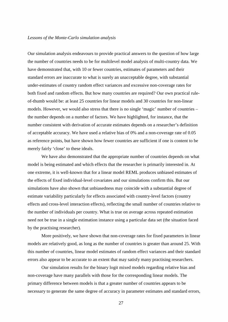
27
Lessons of the Monte-Carlo simulation analysis
Our simulation analysis endeavours to provide practical answers to the question of how large
the number of countries needs to be for multilevel model analysis of multi-country data. We
have demonstrated that, with 10 or fewer countries, estimates of parameters and their
standard errors are inaccurate to what is surely an unacceptable degree, with substantial
under-estimates of country random effect variances and excessive non-coverage rates for
both fixed and random effects. But how many countries are required? Our own practical rule-
of-thumb would be: at least 25 countries for linear models and 30 countries for non-linear
models. However, we would also stress that there is no single ‘magic’ number of countries –
the number depends on a number of factors. We have highlighted, for instance, that the
number consistent with derivation of accurate estimates depends on a researcher’s definition
of acceptable accuracy. We have used a relative bias of 0% and a non-coverage rate of 0.05
as reference points, but have shown how fewer countries are sufficient if one is content to be
merely fairly ‘close’ to these ideals.
We have also demonstrated that the appropriate number of countries depends on what
model is being estimated and which effects that the researcher is primarily interested in. At
one extreme, it is well-known that for a linear model REML produces unbiased estimates of
the effects of fixed individual-level covariates and our simulations confirm this. But our
simulations have also shown that unbiasedness may coincide with a substantial degree of
estimate variability particularly for effects associated with country-level factors (country
effects and cross-level interaction effects), reflecting the small number of countries relative to
the number of individuals per country. What is true on average across repeated estimation
need not be true in a single estimation instance using a particular data set (the situation faced
by the practising researcher).
More positively, we have shown that non-coverage rates for fixed parameters in linear
models are relatively good, as long as the number of countries is greater than around 25. With
this number of countries, linear model estimates of random effect variances and their standard
errors also appear to be accurate to an extent that may satisfy many practising researchers.
Our simulation results for the binary logit mixed models regarding relative bias and
non-coverage have many parallels with those for the corresponding linear models. The
primary difference between models is that a greater number of countries appears to be
necessary to generate the same degree of accuracy in parameter estimates and standard errors,

28
other things being equal. In particular for random coefficient variances (if specified) and
especially the country-level variance, at least 30 to 35 countries may be required to derive
sufficiently accurate estimates – which is more than is usually available (see Table 1).
An additional warning concerning non-linear mixed models in general and the binary
logit mixed model in particular is that the estimator used for maximization also matters. We
have used adaptive Gaussian quadrature, which has been found to produce more accurate
estimates than penalized quasi-likelihood (Rodriguez and Goldman 2001, Pinheiro and Chao
2006, Austin 2010). Other researchers have shown that Bayesian estimation methods using
Markov chain Monte-Carlo methods also perform well, especially with a relatively small
number of ‘countries’ (Austin 2010; Browne and Draper 2000, 2006; Stegmueller 2013).
8. Empirical illustration: hours worked and work participation
Following the Monte Carlo analysis, and to illustrate the practical consequences of using
multilevel data with a small number of countries, we present a simple but representative
application based on data from a commonly-used dataset, EU-SILC.22 Since the Monte Carlo
simulations indicated that we could expect substantial problems with around 10 countries, we
randomly selected 10 from the available 26 countries.23 We estimate models of the form
specified in Table 2, that is linear models of working hours and non-linear (binary logit)
models of work participation. We focus the discussion here on the Basic specification
containing country-specific intercepts but common slopes across countries. (Results for an
Extended specification are available from the authors on request.)
Linear model
The dependent variable in the linear model is the usual number of total weekly hours worked
in the main job of person (woman) i in country c and the explanatory variables are: ageic and
age-squaredic; cohabic, a dummy variable indicating whether a woman is married/cohabiting;
nownchic, number of own children; three iscedic dummy variables indicating highest
22 We use data from 2007, 4th release, which contains 26 countries: the 27 EU member states excluding Bulgaria, Malta and Romania, plus Iceland and Norway. 23 The 10 countries are: Denmark, Estonia, Germany, Hungary, Finland, France, Netherlands, Poland, Portugal, United Kingdom.
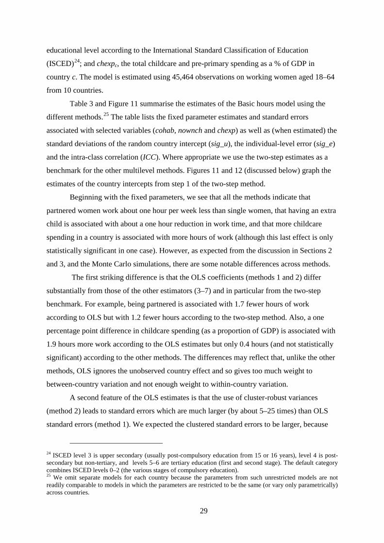
29
educational level according to the International Standard Classification of Education
(ISCED)24; and chexpc, the total childcare and pre-primary spending as a % of GDP in
country c. The model is estimated using 45,464 observations on working women aged 18–64
from 10 countries.
Table 3 and Figure 11 summarise the estimates of the Basic hours model using the
different methods.25 The table lists the fixed parameter estimates and standard errors
associated with selected variables (cohab, nownch and chexp) as well as (when estimated) the
standard deviations of the random country intercept (sig_u), the individual-level error (sig_e)
and the intra-class correlation (ICC). Where appropriate we use the two-step estimates as a
benchmark for the other multilevel methods. Figures 11 and 12 (discussed below) graph the
estimates of the country intercepts from step 1 of the two-step method.
Beginning with the fixed parameters, we see that all the methods indicate that
partnered women work about one hour per week less than single women, that having an extra
child is associated with about a one hour reduction in work time, and that more childcare
spending in a country is associated with more hours of work (although this last effect is only
statistically significant in one case). However, as expected from the discussion in Sections 2
and 3, and the Monte Carlo simulations, there are some notable differences across methods.
The first striking difference is that the OLS coefficients (methods 1 and 2) differ
substantially from those of the other estimators (3–7) and in particular from the two-step
benchmark. For example, being partnered is associated with 1.7 fewer hours of work
according to OLS but with 1.2 fewer hours according to the two-step method. Also, a one
percentage point difference in childcare spending (as a proportion of GDP) is associated with
1.9 hours more work according to the OLS estimates but only 0.4 hours (and not statistically
significant) according to the other methods. The differences may reflect that, unlike the other
methods, OLS ignores the unobserved country effect and so gives too much weight to
between-country variation and not enough weight to within-country variation.
A second feature of the OLS estimates is that the use of cluster-robust variances
(method 2) leads to standard errors which are much larger (by about 5–25 times) than OLS
standard errors (method 1). We expected the clustered standard errors to be larger, because
24 ISCED level 3 is upper secondary (usually post-compulsory education from 15 or 16 years), level 4 is post-secondary but non-tertiary, and levels 5–6 are tertiary education (first and second stage). The default category combines ISCED levels 0–2 (the various stages of compulsory education). 25 We omit separate models for each country because the parameters from such unrestricted models are not readily comparable to models in which the parameters are restricted to be the same (or vary only parametrically) across countries.

30
they account for within-country correlation across individuals, but we also noted above that
cluster-robust methods may not work well with only a few countries. This warning appears to
be borne out by a comparison of the clustered standard errors with those from the other
methods that take proper account of the multilevel data structure. In particular, the standard
errors associated with the two individual-level variables from methods 3–7 are almost the
same as the (uncorrected) OLS standard errors. This suggests that clustered standard errors at
the individual level may be too large, rather than too small, when number of countries is
small.26 In contrast, the clustered standard errors at associated with the country-level
regressor are much closer to those from the other methods.
Next, we compare the fixed parameters estimated by methods 3–7 which account
explicitly for the multilevel structure of the data. We take the two-step estimates (method 7)
as a benchmark (noting that step 1, method 7a, is identical to the country FE approach,
method 3). The point estimates of the fixed parameters, both for individual- and country-level
regressors, are almost identical across the methods and the same as the two-step method,
consistent with them being unbiased. The Monte Carlo simulations of the REML estimator
indicated that the fixed parameter estimates were unbiased even for small group sizes.
We also see that the three random effects estimators (GLS, REML and FML) yield
estimates of the effects of the individual-level predictors which are identical (to three decimal
places) to the FE estimates. We expected GLS and FE to be very similar because, given the
large number of individual observations and few countries, the GLS estimator uses almost
entirely within-country variation. In addition, the ML estimates of the random effects model
(methods 5–6) are very close to RE GLS. An implication is that, for estimating the fixed
parameters associated with individual-level predictors, it does not matter whether the country
intercept is modelled as fixed or random.
The Monte Carlo simulations indicated that there should be little bias in the standard
errors of the parameter estimates on the individual-level predictors, but some downward bias
in the standard error of the parameter estimate of the country-level predictor (although only
about 2% at C = 10, Figure 2). Consistent with expectations, the standard errors of the
individual-level fixed parameters are identical across methods 3–7. But for the country-level
predictor, chexpc, the standard error is 5.35 using step 2 of the two-step (method 7b) ,
compared to 4.79 using REML (method 6). This represents a difference of some 11% (rather
26 A caveat is that cluster-robust standard errors allow for a more general form of within-country correlation than implied by a country intercept common to all individuals.

31
larger than expected) and would lead to higher likelihood of finding a significant effect of
child expenditure using REML rather than the two-step method (although in this example
both are insignificant at conventional significance levels). Of the other estimators, FML gives
the same standard error for the chexpc parameter as REML, but GLS gives a slightly larger
standard error even than the two-step method.
The final group of estimates are the variances of the random components. The Monte
Carlo simulations and earlier research suggest that the estimate of sig_e should be unbiased
but that sig_u should be underestimated (perhaps by some 3%, Figure 1), leading to
underestimates of ICC. Methods 3–7 give identical estimates of sig_e. Step 2 of the two-step
(method 7b) gives a benchmark estimate of sig_u of 4.86, while the REML and FML
estimates are both 4.34 (11% smaller) and the GLS estimate is 4.87 (0.3% larger). Again the
difference between the two-step results and the REML is somewhat larger than was expected
from the Monte Carlo experiments. There is a corresponding difference between ICC,
estimated as 0.195 by the two-step method (or the almost identical GLS) and as 0.162 by
REML and FML. Finally, the Monte Carlos also indicated that the standard error of the sig_u
estimate would be too small. Both REML and FML produce the same estimate, but we are
unable to compare it with GLS or step 2 of the two-step because Stata does not report
estimates of the standard errors of variance components in linear models.
In view of the small number of country-level observations, an alternative to
estimating the effects of country-level predictors statistically is to use less formal descriptive
or visualisation techniques at the country level (Bowers and Drake 2005). This approach
amounts to replacing step 2 of the two-step method with graphs of the estimated country
intercepts (from step 1 or country FE) or with a verbal description of the differing country
intercepts in terms of national institutions. In Figure 11 we plot the estimated country
intercepts against childcare spending (these are the data points used in the step 2 regression).
Consistent with the statistically insignificant chexp estimate of Table 3, there does not appear
to be a systemic association between childcare spending and the country average level of
work hours (adjusted for national differences in age, partnership rates, numbers of children
and education). However, the advantage using visual techniques is to allow a richer (and
perhaps more realistic) view of cross-national variation that may reveal patterns that are
hidden by a simple ‘summary’ regression coefficient. As an illustration, the graph
distinguishes between countries in North-West Europe, Southern European, Eastern Europe
and Scandinavia (Nordic countries). The sample size is small but nevertheless suggestive of
some possible clusters, for instance the NW European group tends to work relatively few

32
hours and spend relatively little on childcare (except for France) while the Nordic countries
have high childcare spending and work relatively long hours (further evidence is provided by
estimates based on 26 countries, available from authors on request). Patterns of this sort in
the data, together with information about country institutions, may lead to the development of
further hypotheses about the determinants of working hours.
Non-linear (binary logit) model
The estimated parameters for the logit model of work participation are presented in Table 4
and Figure 12. The dependent variable is a binary variable equal to one if a women
participates in employment and zero otherwise, with the same explanatory variables as in the
linear model. Estimation is based on the previous sample of workers combined with
additional observations on non-working women (18–64 years), giving a total sample size of
73,169.
From the little evidence cited in previous studies and our Monte Carlo simulations we
expect similar issues to those encountered with the linear model, except that the biases and
excessive non-coverage rates may be worse for small numbers of countries. As before, we
take the two-step results as a benchmark: the point estimates and standard errors of the
individual-level predictor parameters at step 1 should be accurate thanks to large sample sizes
within countries; and the step 2 OLS estimates of the country-level predictor parameter and
country intercept variance should be unbiased (with the correct standard error on the country-
level predictor parameter).
As for the linear model, the fixed parameter estimates from the pooled models
(methods 1–2) differ from multilevel estimates (methods 3–6), although by less than in the
linear case.27 The largest proportionate difference is for the parameter on cohab, which is
0.10 in the pooled model but only 0.07 in the multilevel models. The unclustered standard
errors of the individual-level predictor effects are almost identical to those of the multilevel
models, but (as in the linear case) the unclustered standard error for the country-level
predictor effect is much smaller in the pooled estimates (0.032 compared with 0.284 in the
27 The estimates from the pooled and the multilevel logits are not directly comparable because: (a) the composite error term in the pooled logit, uc + εic, is assumed to follow the logistic distribution, while in the random effects logit uc is assumed to be normal and only εic has a logistic distribution; (b) the estimated fixed parameters are scaled by 1/sd(uc + εic) in the pooled logit, but only by 1/sd(εic) in the multilevel logit. To make the scaling comparable, it is easily shown that the multilevel parameters should be multiplied by √(1 – ICC). In our example, ICC = 0.020 and so the multiplication factor is 0.992, a trivial adjustment which, nevertheless, increases very slightly the difference between the two sets of estimates.

33
two-step method). The use of clustering brings the country-level predictor standard error
almost up to those of methods 3–6, but (as in the linear model) clustering appears to overstate
the standard errors of the individual-level predictor parameters (for example, the standard
error of the nownch parameter is 0.045 in the pooled estimates, but only 0.01 in the multilevel
estimates). This again suggests that clustered standard errors may lead to misleading
conclusions with small numbers of groups.
Focussing on the methods that account for the multilevel data structure, we see that
the estimated fixed parameters from the RE and MLM (FML) logits are almost identical to
the two-step estimates, consistent with the negligible parameter bias found in the Monte
Carlo simulations. The estimates of the FE logit are also the same as the corresponding
estimates from the RE logit, indicating (as for the linear model) that the choice between FE
and RE is unimportant if interest focuses on the individual-level predictors.
Turning to the standard errors on the estimated fixed parameters, we see that they are
identical across methods 3–6 for the individual-level predictors but not for country-level
regressor. From the Monte Carlo simulations, we expected the standard error on the chexp
parameter to be downward biased by about 15% (Figure 7). The ‘benchmark’ standard error
from the two-step method is 0.284, while the RE and MLM standard errors are both 0.255,
implying that they are understated by 10%. This is somewhat less than expected from the
Monte Carlos, but in this example we will see that it is enough to change the conclusion
about the effect of national childcare spending on work participation.
The corresponding test statistics for the effect of chexp are 0.529/0.255 = 2.07 from
the RE and MLM models, and 0.529/0.284 = 1.86 from the two-step method. If the RE/MLM
test statistic is referred to the standard normal distribution, then the p-value, as reported by
Stata, is 0.038. Thus the chexp estimate is significant at the 5% level. By contrast the p-value
of the two-step test statistic, referred to the t(8)-distribution and as reported by Stata, is
0.100.28 Therefore the estimated parameter is not significant at the 5% level and not quite
significant even at the 10% level. We see how an underestimate of the standard error in the
MLM leads to an overly liberal conclusion. A more conservative strategy may be to use the t-
distribution instead of the normal as a reference for the MLM estimates (Raudenbush and
Bryk 2002: 282). Using the t(8)-distribution, the p-value of the RE/MLM test statistic is
0.072, so the estimated effect is no longer significant at the 5% level, although it is still
28 Step 2 of the two-step method is an OLS regression using 10 country observations. The 8 degrees of freedom are equal to 10 observations minus a constant and one country-level regressor.

34
significant at 10%. However, since most statistical software reports p-values based on an
asymptotic normal distribution (an exception is HLM), this correction needs to be done
manually by users.
Lastly, we compare the standard deviation of the random intercept, as estimated by
the RE and MLM methods and the two-step method. From the Monte Carlos simulations, we
expect sig_u to be downward biased by about 15%. The gap in the estimates is somewhat less
but nevertheless quite substantial: the RE and MLM estimates (0.229) are 11% less than the
two-step estimate (0.258). The difference leads to a correspondingly lower value of ICC in
RE/MLM (0.016) than two-step (0.020).
For a graphical view of country-level variation, the country-specific intercepts are
plotted against national childcare expenditure in Figure 12. There is a clearer upward slope
than for hours worked, suggesting that more childcare spending may be associated with
greater work participation, although the data point for Denmark may be exerting undue
influence. There is somewhat less evidence of distinct country clusters than in the working
hours model, although Finland and Denmark have high participation rates (also high levels of
childcare spending).
9. Summary and conclusions
When there are few countries in a multi-country data set, there is little information with
which to estimate country effects, whether these effects refer to the fixed parameters on
country-level predictors or the variances of random country intercepts. Multilevel model
users need to be cautious in the claims they make about country effects.
Our Monte-Carlo simulations suggest that users require at least 25 countries for linear
models and at least 30 countries for logit models. With fewer countries, estimates of country-
level fixed parameters are likely to be estimated imprecisely and this will not be adequately
reflected in test statistics reported by commonly-used software: users will conclude too often
that a country effect exists when it does not. Country random variances will be biased
downwards and have confidence intervals that are too narrow. The only estimates that are
unaffected by the small number of countries are the fixed parameters on individual-level
predictors (the number of individuals per country is typically large): provided there is not also
a random component attached to the slope, these parameters are estimated without bias and
with the correct standard errors (and non-coverage rate).

35
Since the critical number of countries required for reliable estimation of country effects is
larger than is available in many existing datasets, what can analysts do in the small-C case?
We recommend three approaches. One is to supplement regression-based modelling with
more descriptive analysis of measured country differences. We have referred to exploratory
data analysis, including graphical representations of country differences, which may reveal
features of the data (including outliers and country groupings) that are hidden when fitting a
simple regression line. A second approach is to explore methods that are more robust to small
numbers of countries. These include the two-step method, small sample corrections to test
statistics, and bootstrapping; although some of these techniques require specialised
knowledge and are available in only a few software packages. A third approach would be to
move beyond classical (frequentist) statistics and make greater use of Bayesian methods of
estimation and inference, as they appear to perform better in the small-C case. The problem is
that these methods also require statistical expertise beyond that of most applied social science
researchers, as well as specialist software. With any of these approaches, the need for detailed
consideration of the workings of national institutions and policies remains.
References
Aachen, C. H. (2005). ‘Two-step hierarchical estimation: beyond regression analysis’,
Political Analysis, 13, 447–456.
Angrist, J. D. and Pischke, J.-S. (2009). Mostly Harmless Econometrics: An Empiricist’s
Companion. Princeton NJ: Princeton University Press.
Austin, P. C. (2010). ‘Estimating multilevel logistic regression models when the number of
clusters is low: a comparison of different statistical software procedures’,
International Journal of Biostatistics, 6, article 16.
Beck, N. and Katz, J. N. (1995). ‘What to do (and not to do) with time-series cross-section
data’, American Political Science Review, 89, 634–647.
Bell, R. M. and McCaffrey, D. F. (2002). ‘Bias reduction in standard errors for linear
regression with multistage samples’, Survey Methodology, 28, 169–181.
Bester, C. A., Conley, T. G., Hansen, C. B. (2011). ‘Inference with dependent data using
cluster covariance estimators’, Journal of Econometrics, 165, 137–151.
Borjas, G. J. and Sueyoshi, G. T. (1994). ‘A two-stage estimator for probit models with
structural group effects’, Journal of Econometrics, 64,165–182.

36
Bowers, J. and Drake, K. W. (2005). ‘EDA for HLM: visualization when probabilistic
inference fails’, Political Analysis, 13, 301–326.
Brewer, M., Crossley, T. F., and Joyce, R. (2013). ‘Inference with Difference-in-Differences
Revisited’. Paper for the 8th IZA Conference on Labor Market Evaluation, London.
http://www.iza.org/conference_files/PolicyEval_2013/joyce_r8616.pdf
Browne, W. C. and Draper, D. (2000). ‘Implementation and performance issues in Baysian
and likelihood fitting of multilevel models’, Computational Statistics, 15, 391–420.
Browne, W. J., and Draper, D. (2006). ‘A comparison of Bayesian and likelihood-based
methods for fitting multilevel models’, Bayesian Analysis, 1, 473–514.
Cameron, C. A., Gelbach, J. B., and Miller, D. L. (2008). ‘Bootstrap-based improvements for
inference with clustered standard errors’, Review of Economics and Statistics, 90,
414–427.
Cameron, C. A., and Trivedi P. K. (2010), Microeconometrics using Stata, revised edition.
College Station TX: Stata Press.
Card, D. (1995). ‘The wage curve: a review’, Journal of Economic Literature, 33, 285–299.
Carpenter, J. R., Goldstein, H., and Rasbash, J. (2003). ‘A novel bootstrap procedure for
assessing the relationship between class size and achievement’, Journal of the Royal
Statistical Society, Series C, 52, 431–443.
DiPrete, T. A. and Forristal, J. D. (1994). ‘Multilevel models: methods and substance’,
Annual Review of Sociology, 20, 331–357.
Donald, S. G. and Lang, K. (2007). ‘Inference with difference-in-differences and other panel
data’, Review of Economics and Statistics, 89, 221–233.
Gelman, A. (2006). ‘Prior distributions for variance parameters in hierarchical models’,
Bayesian Analysis, 1, 515–533.
Greene, W. (2004). ‘The behaviour of the maximum likelihood estimator of limited
dependent variable models in the presence of fixed effects’, Econometrics Journal, 7,
98–119.
Hanushek, E. A. (1974). ‘Efficient estimators for regressing regression coefficients’,
American Statistician, 28, 66–67.
Hox, J. J. (2010), Multilevel Analysis: Techniques and Applications, 2nd edition. London:
Routledge.
Hsiao, C. (2003). Analysis of Panel Data, 2nd edition. Cambridge: Cambridge University
Press.

37
Huber, J. D., Kernell, G., and Leoni, E. (2005). ‘Institutional context, cognitive resources and
partisan attachments across democracies’, Political Analysis, 13, 365–386.
Jusko, K. L., and Shively, W. P. (2005). ‘A two-step strategy for the analysis of cross-
national public opinion data’, Political Analysis, 13, 327–344.
Kedar, O. (2005). ‘How diffusion of power in parliaments affects voter choice’, Political
Analysis, 13, 410–429.
Kedar, O. and Shively, W. P. (2005). ‘Introduction to the special issue’, Political Analysis,
13, 297–300.
Kenward, M. G and Roger, J. H. (1997). ‘Small sample inference for fixed effects from
restricted maximum likelihood’, Biometrics, 53, 983–997.
Maas, C. J. M. and Hox, J. J. (2004). ‘Robustness issues in multilevel regression analysis’,
Statistica Neerlandica, 58, 127–137.
Maas, C. J. M. and Hox, J. J. (2005). ‘Sufficient sample sizes for multilevel modeling’,
Methodology, 1, 86–92.
Moineddin, R., Matheson, F. I., and Glazier, R. H. (2007). ‘A simulation study of sample size
in multilevel regression models’, BMC Medical Research Methodology, 7: article 34.
Moulton, B. R. (1986). ‘Random group effects and the precision of regression estimates,’
Journal of Econometrics, 32, 385–397.
Pinheiro, J. C. and Chao, E. C. (2006). ‘Efficient Laplacian and adaptive quadrature
algorithms for multilevel generalized linear mixed models’, Journal of Computational
and Graphical Statistics, 15, 58–81.
Raudenbush, S. W. and Bryk, A. S. (2002). Hierarchical Linear Models: Applications and
Data Analysis Methods, Second Edition. Thousand Oaks CA: Sage Publications.
Raudenbush S. W., Bryk, A. S., Cheong, Y. F., and Congdon, R. T. Jr. (2004). HLM 6:
Hierarchical Linear and Nonlinear Modeling. Lincolnwood IL: Scientific Software
International.
Rodriguez, G. and Goldman, N. (1995). ‘An assessment of estimation procedures for
multilevel models with binary responses’, Journal of the Royal Statistical Society,
Series A, 158, 73–89.
Rodriguez, G. and Goldman, N. (2001). ‘Improved estimation procedures for multilevel
models with binary response: case study’, Journal of the Royal Statistical Society,
Series A, 164, 339–355.
Saxonhouse, G. R. (1976). ‘Estimated parameters as dependent variables’, American
Economic Review, 66, 178–183.

38
Snijders, T. A.B. and Bosker, R. (1999). Multilevel Analysis: An Introduction to Basic and
Advanced Multilevel Modeling. Thousand Oaks CA: Sage Publications Ltd.
StataCorp (2011). Stata Statistical Software, Release 12. College Station, TX: StataCorp.
Stegmueller, D. (2013). ‘How many countries do you need for multilevel modeling? A
comparison of Bayesian and frequentist approaches’, American Journal of Political
Science, 57, 748–761.
Wang,J., Carpenter, J. R., and Kepler, M. A. (2006). ‘Using SAS to conduct nonparametric
residual bootstrap multilevel modeling with a small number of groups’, Computer
Methods and Programs in Biomedicine, 82, 130–143. With Corrigendum, 85(2007)
185–186.
Wooldridge, J. (2010). Econometric Analysis of Cross Section and Panel Data, 2nd edition.
Cambridge MA: MIT Press.
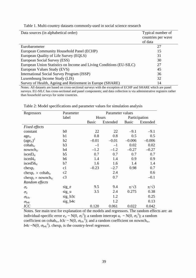
39
Table 1. Multi-country datasets commonly-used in social science research
Data sources (in alphabetical order) Typical number of countries per wave of data
Eurobarometer 27 European Community Household Panel (ECHP) 15 European Quality of Life Survey (EQLS) 31 European Social Survey (ESS) 30 European Union Statistics on Income and Living Conditions (EU-SILC) 27 European Values Study (EVS) 45 International Social Survey Program (ISSP) 36 Luxembourg Income Study (LIS) 32 Survey of Health, Ageing and Retirement in Europe (SHARE) 14 Notes: All datasets are based on cross-sectional surveys with the exception of ECHP and SHARE which are panel surveys. EU-SILC has cross-sectional and panel components; and data collection is via administrative registers rather than household surveys for some countries.
Table 2: Model specifications and parameter values for simulation analysis
Regressors Parameter Parameter values label Hours Participation Basic Extended Basic Extended Fixed effects constant b0 22 22 –9.1 –9.1 ageic b1 0.8 0.8 0.5 0.5 (ageic)2 b2 –0.01 –0.01 –0.006 –0.006 cohabic b3 –1 –1 0.02 0.02 nownchic b4 –1.2 –1.2 –0.27 –0.27 isced3ic b5 0.7 0.7 0.7 0.7 isced4ic b6 1.4 1.4 0.9 0.9 isced56ic b7 1.6 1.6 1.4 1.4 chexpc c1 –0.23 –2.7 0.98 0.7 chexpc × cohabic c2 2.4 0.6 chexpc × nownchic c3 0.7 –0.1 Random effects σe sig_e 9.5 9.4 π/√3 π/√3 σu sig_u 3.5 2.4 0.275 0.38 σb3c sig_b3c 1.2 0.25 σb4c sig_b4c 1.2 0.13 ICC 0.120 0.061 0.022 0.042 Notes. See main text for explanation of the models and regressors. The random effects are: an individual-specific error eic ~ N(0, σe
2); a random intercept uc ~ N(0, σu2); a random
coefficient on cohabic, b3c ~ N(0, σb3c2); and a random coefficient on nownchic,
b4c ~N(0, σb4c2). chexpc is the country-level regressor.

40
Table 3. Model of working hours with country-specific intercepts: alternative estimation methods compared
Parameter estimates (standard errors) Method cohabic nownchic chexpc sig_u sig_e ICC 1. OLS –1.651*** –1.177*** 1.876***
(0.125) (0.055) (0.184) 2. OLS (clust SE) –1.651* –1.177* 1.876 (0.836) (0.586) (4.351) 3. FE –1.151*** –1.585***
9.881
(0.114) (0.051) 4. RE (GLS ) –1.152*** –1.585*** 0.423 4.872 9.881 0.196
(0.114) (0.051) (5.370) 5. MLM (REML) –1.152*** –1.585*** 0.424 4.341*** 9.880*** 0.162
(0.114) (0.051) (4.785) (0.972) (0.033) 6. MLM (FML) –1.152*** –1.585*** 0.424 4.341*** 9.880*** 0.162
(0.114) (0.051) (4.785) (0.972) (0.033) 7a. Step 1 (FE) –1.151*** –1.585***
9.881
(0.114) (0.051) 7b. Step 2 (OLS)
0.421 4.856
0.195
(5.349)
Notes: other explanatory variables are: age, age squared, and highest education level (3 dummy variables); number of observations is 45,464 and number of countries is 10; * significant at 10%; ** significant at 5%; *** significant at 1%.
Table 4. Model of work participation with country-specific intercepts: alternative estimation methods compared
Parameter estimates (standard errors) Method cohabic nownchic chexpc sig_u ICC 1. Pooled logit 0.100*** -0.294*** 0.583***
(0.021) (0.009) (0.032) 2. Pooled logit (clust SE) 0.100* -0.294*** 0.583** (0.059) (0.045) (0.252) 3. FE logit 0.071*** -0.288***
(0.021) (0.010) 4. RE logit 0.072*** -0.288*** 0.529** 0.229*** 0.016
(0.021) (0.010) (0.255) (0.052) 5. MLM logit (FML) 0.072*** -0.288*** 0.529** 0.229*** 0.016
(0.021) (0.010) (0.255) (0.052) 6a. Step 1 0.071*** -0.288***
(0.021) (0.010) 6b. Step 2 (OLS)
0.529 0.258 0.020
(0.284)
Notes: other explanatory variables are: age, age squared, and highest education level (3 dummy variables); number of observations is 73,169 and number of countries is 10; * significant at 10%; ** significant at 5%; *** significant at 1%; for methods 1–6a, significance levels are as reported by Stata, and refer to critical values from z-distribution; for method 6b, significance levels refer to critical values from t(8)-distribution.
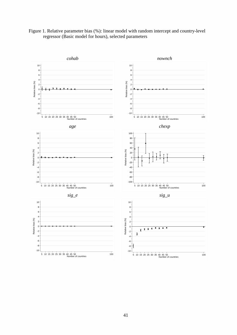
41
Figure 1. Relative parameter bias (%): linear model with random intercept and country-level regressor (Basic model for hours), selected parameters
cohab nownch
age chexp
sig_e sig_u
-10
-8
-6
-4
-2
0
2
4
6
8
10
Rel
ativ
e bi
as (%
)
5 10 15 20 25 30 35 40 45 50 100Number of countries
-10
-8
-6
-4
-2
0
2
4
6
8
10
Rel
ativ
e bi
as (%
)
5 10 15 20 25 30 35 40 45 50 100Number of countries
-10
-8
-6
-4
-2
0
2
4
6
8
10
Rel
ativ
e bi
as (%
)
5 10 15 20 25 30 35 40 45 50 100Number of countries
-100
-80
-60
-40
-20
0
20
40
60
80
100
Rel
ativ
e bi
as (%
)
5 10 15 20 25 30 35 40 45 50 100Number of countries
-10
-8
-6
-4
-2
0
2
4
6
8
10
Rel
ativ
e bi
as (%
)
5 10 15 20 25 30 35 40 45 50 100Number of countries
-10
-8
-6
-4
-2
0
2
4
6
8
10
Rel
ativ
e bi
as (%
)
5 10 15 20 25 30 35 40 45 50 100Number of countries

42
Figure 2. Relative standard error bias: linear model with random intercept and country-level regressor (Basic model for hours), selected parameters
-25
-20
-15
-10
-5
0
5
Rel
ativ
e di
ffere
nce
(%)
0 5 10 15 20 25 30 35 40 45 50 100Number of countries
age cohab nownchchexp sig_u sig_e

43
Figure 3. Non-coverage rate: linear model with random intercept and country-level regressor (Basic model for hours), selected parameters
cohab nownch
age chexp
sig_e sig_u
0.00
0.02
0.04
0.06
0.08
0.10
0.12
0.14
0.16
0.18
0.20
Non
-cov
erag
e ra
te
5 10 15 20 25 30 35 40 45 50 100Number of countries
0.00
0.02
0.04
0.06
0.08
0.10
0.12
0.14
0.16
0.18
0.20
Non
-cov
erag
e ra
te
5 10 15 20 25 30 35 40 45 50 100Number of countries
0.00
0.02
0.04
0.06
0.08
0.10
0.12
0.14
0.16
0.18
0.20
Non
-cov
erag
e ra
te
5 10 15 20 25 30 35 40 45 50 100Number of countries
0.00
0.02
0.04
0.06
0.08
0.10
0.12
0.14
0.16
0.18
0.20
Non
-cov
erag
e ra
te
5 10 15 20 25 30 35 40 45 50 100Number of countries
0.00
0.02
0.04
0.06
0.08
0.10
0.12
0.14
0.16
0.18
0.20
Non
-cov
erag
e ra
te
5 10 15 20 25 30 35 40 45 50 100Number of countries
0.00
0.02
0.04
0.06
0.08
0.10
0.12
0.14
0.16
0.18
0.20
Non
-cov
erag
e ra
te
5 10 15 20 25 30 35 40 45 50 100Number of countries

44
Figure 4. Relative parameter bias (%): linear model with random intercept, two random slopes, country-level regressor and individual-country interaction (Extended model for hours), selected parameters
cohab nownch
age chexp
chexpXcohab chexpXnownch
Continued overleaf
-10
-8
-6
-4
-2
0
2
4
6
8
10
Rel
ativ
e bi
as (%
)
5 10 15 20 25 30 35 40 45 50 100Number of countries
-10
-8
-6
-4
-2
0
2
4
6
8
10
Rel
ativ
e bi
as (%
)
5 10 15 20 25 30 35 40 45 50 100Number of countries
-10
-8
-6
-4
-2
0
2
4
6
8
10
Rel
ativ
e bi
as (%
)
5 10 15 20 25 30 35 40 45 50 100Number of countries
-10
-8
-6
-4
-2
0
2
4
6
8
10
Rel
ativ
e bi
as (%
)
5 10 15 20 25 30 35 40 45 50 100Number of countries
-10
-8
-6
-4
-2
0
2
4
6
8
10
Rel
ativ
e bi
as (%
)
5 10 15 20 25 30 35 40 45 50 100Number of countries
-10
-8
-6
-4
-2
0
2
4
6
8
10
Rel
ativ
e bi
as (%
)
5 10 15 20 25 30 35 40 45 50 100Number of countries

45
Figure 4 (continued). Relative parameter bias (%): model with random intercept, two random slopes, country-level regressor and individual-country interaction (Extended model for hours), selected parameters
sig_b3c sig_b4c
sig_e sig_u
-16
-14
-12
-10
-8
-6
-4
-2
0
2
4
6
8
10
Rel
ativ
e bi
as (%
)
5 10 15 20 25 30 35 40 45 50 100Number of countries
-16
-14
-12
-10
-8
-6
-4
-2
0
2
4
6
8
10
Rel
ativ
e bi
as (%
)5 10 15 20 25 30 35 40 45 50 100
Number of countries
-10
-8
-6
-4
-2
0
2
4
6
8
10
Rel
ativ
e bi
as (%
)
5 10 15 20 25 30 35 40 45 50 100Number of countries
-10
-8
-6
-4
-2
0
2
4
6
8
10
Rel
ativ
e bi
as (%
)
5 10 15 20 25 30 35 40 45 50 100Number of countries

46
Figure 5. Non-coverage rate: model with random intercept, two random slopes, country-level regressor and individual-country interaction (Extended model for hours), selected parameters
cohab nownch
age chexp
chexpXcohab chexpXnownch
Continued overleaf
0.00
0.02
0.04
0.06
0.08
0.10
0.12
0.14
0.16
0.18
0.20
Non
-cov
erag
e ra
te
5 10 15 20 25 30 35 40 45 50 100Number of countries
0.00
0.02
0.04
0.06
0.08
0.10
0.12
0.14
0.16
0.18
0.20
Non
-cov
erag
e ra
te5 10 15 20 25 30 35 40 45 50 100
Number of countries
0.00
0.02
0.04
0.06
0.08
0.10
0.12
0.14
0.16
0.18
0.20
Non
-cov
erag
e ra
te
5 10 15 20 25 30 35 40 45 50 100Number of countries
0.00
0.02
0.04
0.06
0.08
0.10
0.12
0.14
0.16
0.18
0.20
Non
-cov
erag
e ra
te
5 10 15 20 25 30 35 40 45 50 100Number of countries
0.00
0.02
0.04
0.06
0.08
0.10
0.12
0.14
0.16
0.18
0.20
Non
-cov
erag
e ra
te
5 10 15 20 25 30 35 40 45 50 100Number of countries
0.00
0.02
0.04
0.06
0.08
0.10
0.12
0.14
0.16
0.18
0.20
Non
-cov
erag
e ra
te
5 10 15 20 25 30 35 40 45 50 100Number of countries

47
Figure 5 (continued). Non-coverage rate: linear model with random intercept, two random slopes, country-level regressor and individual-country interaction (Extended model for hours), selected parameters
sig_b3c sig_b4c
sig_u
0.00
0.02
0.04
0.06
0.08
0.10
0.12
0.14
0.16
0.18
0.20
Non
-cov
erag
e ra
te
5 10 15 20 25 30 35 40 45 50 100Number of countries
0.00
0.02
0.04
0.06
0.08
0.10
0.12
0.14
0.16
0.18
0.20
Non
-cov
erag
e ra
te5 10 15 20 25 30 35 40 45 50 100
Number of countries
0.00
0.02
0.04
0.06
0.08
0.10
0.12
0.14
0.16
0.18
0.20
Non
-cov
erag
e ra
te
5 10 15 20 25 30 35 40 45 50 100Number of countries

48
Figure 6. Relative parameter bias (%): binary logit model with random intercept and country-level regressor (Basic model for participation), selected parameters
cohab nownch
age chexp
sig_u
-40
-35
-30
-25
-20
-15
-10
-5
0
5
10
Rel
ativ
e bi
as (%
)
5 10 15 20 25 30 35 40 45 50 100Number of countries
-10
-8
-6
-4
-2
0
2
4
6
8
10
Rel
ativ
e bi
as (%
)
5 10 15 20 25 30 35 40 45 50 100Number of countries
-10
-8
-6
-4
-2
0
2
4
6
8
10
Rel
ativ
e bi
as (%
)
5 10 15 20 25 30 35 40 45 50 100Number of countries
-10
-8
-6
-4
-2
0
2
4
6
8
10
Rel
ativ
e bi
as (%
)
5 10 15 20 25 30 35 40 45 50 100Number of countries
-40
-35
-30
-25
-20
-15
-10
-5
0
5
10
Rel
ativ
e bi
as (%
)
5 10 15 20 25 30 35 40 45 50 100Number of countries

49
Figure 7. Relative standard error bias: binary logit model with random intercept and country-level regressor (Basic model for participation), selected parameters
-25
-20
-15
-10
-5
0
5
Rel
ativ
e di
ffere
nce
(%)
5 10 15 20 25 30 35 40 45 50 100Number of countries
age cohab nownchchexp sig_u

50
Figure 8. Non-coverage rate: binary logit model with random intercept and country-level regressor (Basic model for participation), selected parameters
cohab nownch
age chexp
sig_u
0.00
0.02
0.04
0.06
0.08
0.10
0.12
0.14
0.16
0.18
0.20
Non
-cov
erag
e ra
te
5 10 15 20 25 30 35 40 45 50 100Number of countries
0.00
0.02
0.04
0.06
0.08
0.10
0.12
0.14
0.16
0.18
0.20
Non
-cov
erag
e ra
te
5 10 15 20 25 30 35 40 45 50 100Number of countries
0.00
0.02
0.04
0.06
0.08
0.10
0.12
0.14
0.16
0.18
0.20
Non
-cov
erag
e ra
te
5 10 15 20 25 30 35 40 45 50 100Number of countries
0.00
0.02
0.04
0.06
0.08
0.10
0.12
0.14
0.16
0.18
0.20
Non
-cov
erag
e ra
te
5 10 15 20 25 30 35 40 45 50 100Number of countries
0.00
0.05
0.10
0.15
0.20
0.25
0.30
0.35
0.40
Non
-cov
erag
e ra
te
5 10 15 20 25 30 35 40 45 50 100Number of countries
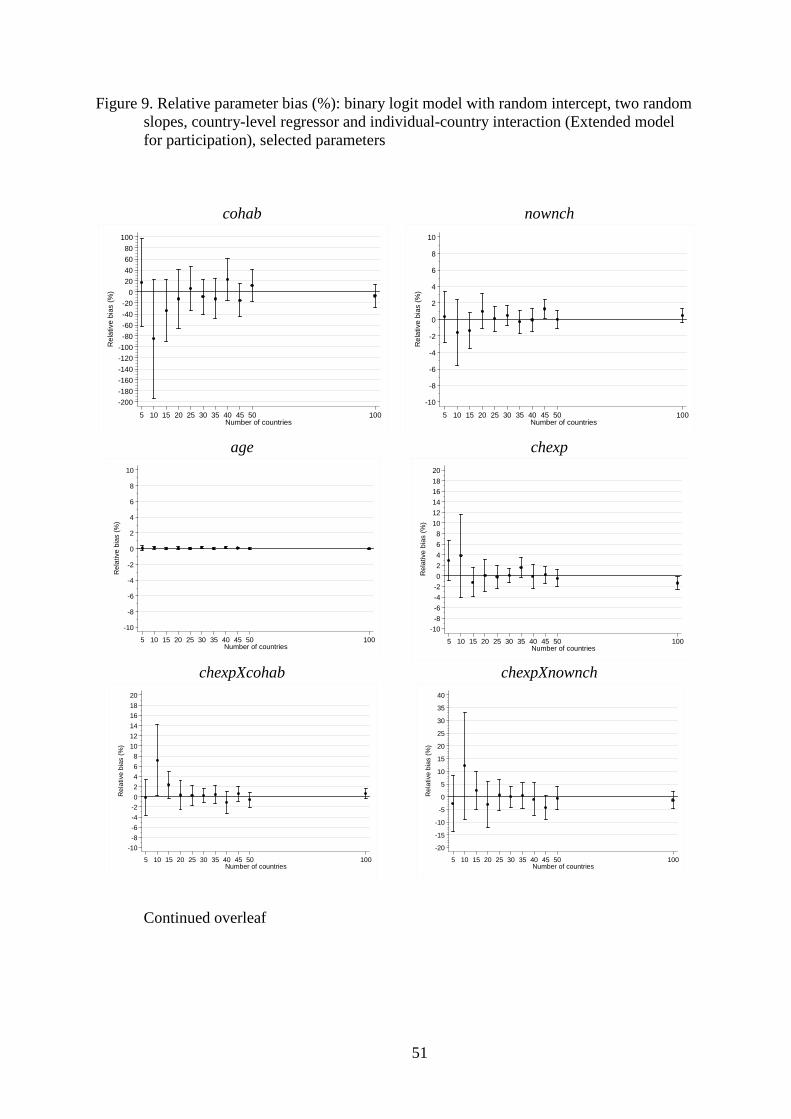
51
Figure 9. Relative parameter bias (%): binary logit model with random intercept, two random slopes, country-level regressor and individual-country interaction (Extended model for participation), selected parameters
cohab nownch
age chexp
chexpXcohab chexpXnownch
Continued overleaf
-200-180-160-140-120-100-80-60-40-20
020406080
100
Rel
ativ
e bi
as (%
)
5 10 15 20 25 30 35 40 45 50 100Number of countries
-10
-8
-6
-4
-2
0
2
4
6
8
10
Rel
ativ
e bi
as (%
)5 10 15 20 25 30 35 40 45 50 100
Number of countries
-10
-8
-6
-4
-2
0
2
4
6
8
10
Rel
ativ
e bi
as (%
)
5 10 15 20 25 30 35 40 45 50 100Number of countries
-10-8-6-4-202468
101214161820
Rel
ativ
e bi
as (%
)
5 10 15 20 25 30 35 40 45 50 100Number of countries
-10-8-6-4-202468
101214161820
Rel
ativ
e bi
as (%
)
5 10 15 20 25 30 35 40 45 50 100Number of countries
-20
-15
-10
-5
0
5
10
15
20
25
30
35
40
Rel
ativ
e bi
as (%
)
5 10 15 20 25 30 35 40 45 50 100Number of countries

52
Figure 9 (continued). Relative parameter bias (%):binary logit model with random intercept, two random slopes, country-level regressor and individual-country interaction (Extended model for participation), selected parameters
sig_b3c sig_b4c
sig_u
-60-55-50-45-40-35-30-25-20-15-10-505
10
Rel
ativ
e bi
as (%
)
5 10 15 20 25 30 35 40 45 50 100Number of countries
-60-55-50-45-40-35-30-25-20-15-10-505
10
Rel
ativ
e bi
as (%
)
5 10 15 20 25 30 35 40 45 50 100Number of countries
-60-55-50-45-40-35-30-25-20-15-10-505
10
Rel
ativ
e bi
as (%
)
5 10 15 20 25 30 35 40 45 50 100Number of countries
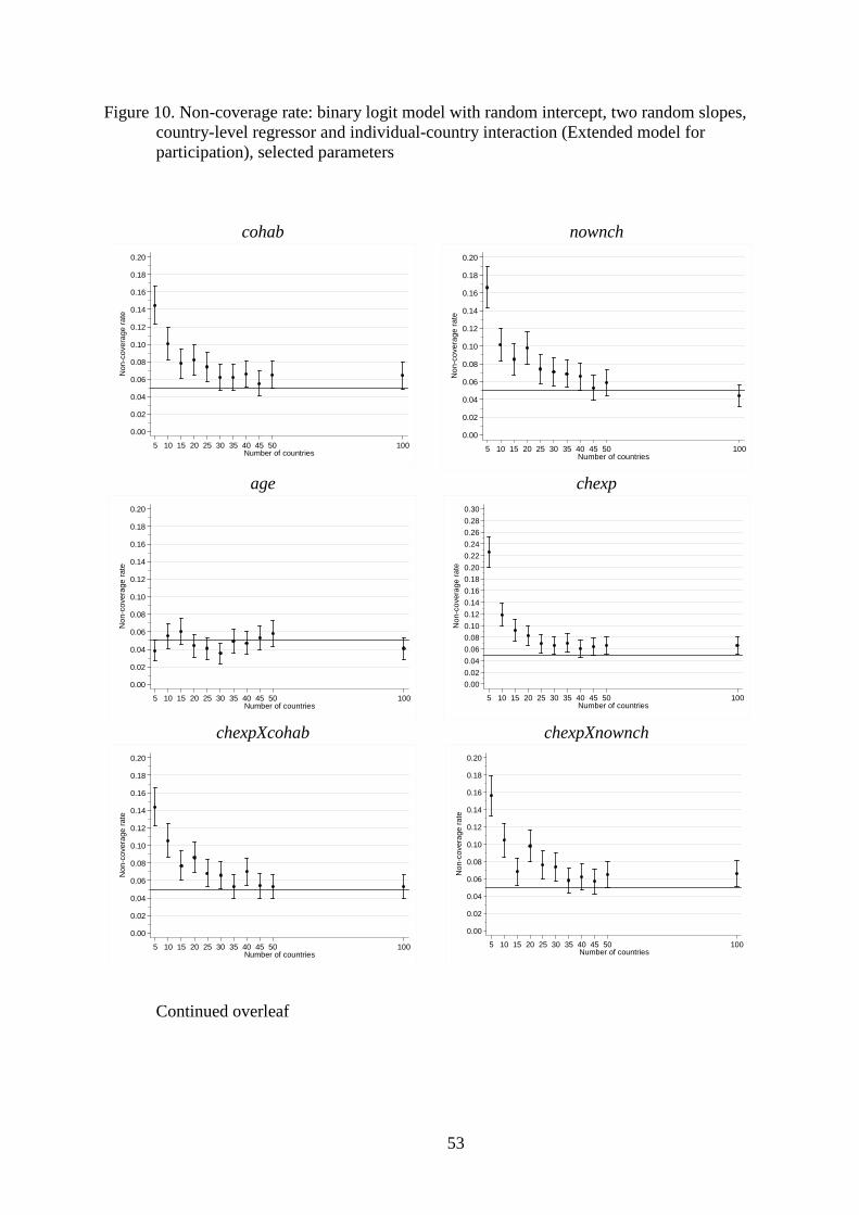
53
Figure 10. Non-coverage rate: binary logit model with random intercept, two random slopes, country-level regressor and individual-country interaction (Extended model for participation), selected parameters
cohab nownch
age chexp
chexpXcohab chexpXnownch
Continued overleaf
0.00
0.02
0.04
0.06
0.08
0.10
0.12
0.14
0.16
0.18
0.20
Non
-cov
erag
e ra
te
5 10 15 20 25 30 35 40 45 50 100Number of countries
0.00
0.02
0.04
0.06
0.08
0.10
0.12
0.14
0.16
0.18
0.20
Non
-cov
erag
e ra
te5 10 15 20 25 30 35 40 45 50 100
Number of countries
0.00
0.02
0.04
0.06
0.08
0.10
0.12
0.14
0.16
0.18
0.20
Non
-cov
erag
e ra
te
5 10 15 20 25 30 35 40 45 50 100Number of countries
0.000.020.040.060.080.100.120.140.160.180.200.220.240.260.280.30
Non
-cov
erag
e ra
te
5 10 15 20 25 30 35 40 45 50 100Number of countries
0.00
0.02
0.04
0.06
0.08
0.10
0.12
0.14
0.16
0.18
0.20
Non
-cov
erag
e ra
te
5 10 15 20 25 30 35 40 45 50 100Number of countries
0.00
0.02
0.04
0.06
0.08
0.10
0.12
0.14
0.16
0.18
0.20
Non
-cov
erag
e ra
te
5 10 15 20 25 30 35 40 45 50 100Number of countries
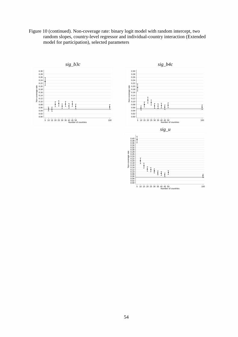
54
Figure 10 (continued). Non-coverage rate: binary logit model with random intercept, two random slopes, country-level regressor and individual-country interaction (Extended model for participation), selected parameters
sig_b3c sig_b4c
sig_u
0.000.020.040.060.080.100.120.140.160.180.200.220.240.260.280.30
Non
-cov
erag
e ra
te
5 10 15 20 25 30 35 40 45 50 100Number of countries
0.000.020.040.060.080.100.120.140.160.180.200.220.240.260.280.30
Non
-cov
erag
e ra
te
5 10 15 20 25 30 35 40 45 50 100Number of countries
0.000.020.040.060.080.100.120.140.160.180.200.220.240.260.280.300.320.340.360.380.40
Non
-cov
erag
e ra
te
5 10 15 20 25 30 35 40 45 50 100Number of countries

55
Figure 11. Model of working hours: country-specific intercepts and childcare/pre-primary spending
Figure 12. Model of work participation: country-specific intercepts and childcare/pre-primary
spending (10 countries)
DE
FR
NL
UK
PT
DK
FI
EEHU
PL
1015
2025
Cou
ntry
inte
rcep
t
.2 .4 .6 .8 1 1.2Total childcare and pre-primary spending as a % of GDP, 2005
NW Europe S EuropeNordic countries E Europe
DE
FR
NLUK
PT
DK
FIEE
HUPL-9
.2-9
-8.8
-8.6
-8.4
-8.2
Cou
ntry
inte
rcep
t
.2 .4 .6 .8 1 1.2Total childcare and pre-primary spending as a % of GDP, 2005
NW Europe S EuropeNordic countries E Europe

56
APPENDIX:
MONTE-CARLO SIMULATION ESTIMATES The following tables summarize the Monte Carlo simulations of the models for hours and participation (Basic and Extended). For each of the four models, we give its specification and summarize the results in two tables: (i) the estimated parameter values and their bias, and (ii) the estimated standard errors and their bias, and the resulting non-coverage rates. The tables provide the estimates underlying Figures 1–10 in the main body of the paper, as well as additional estimates.
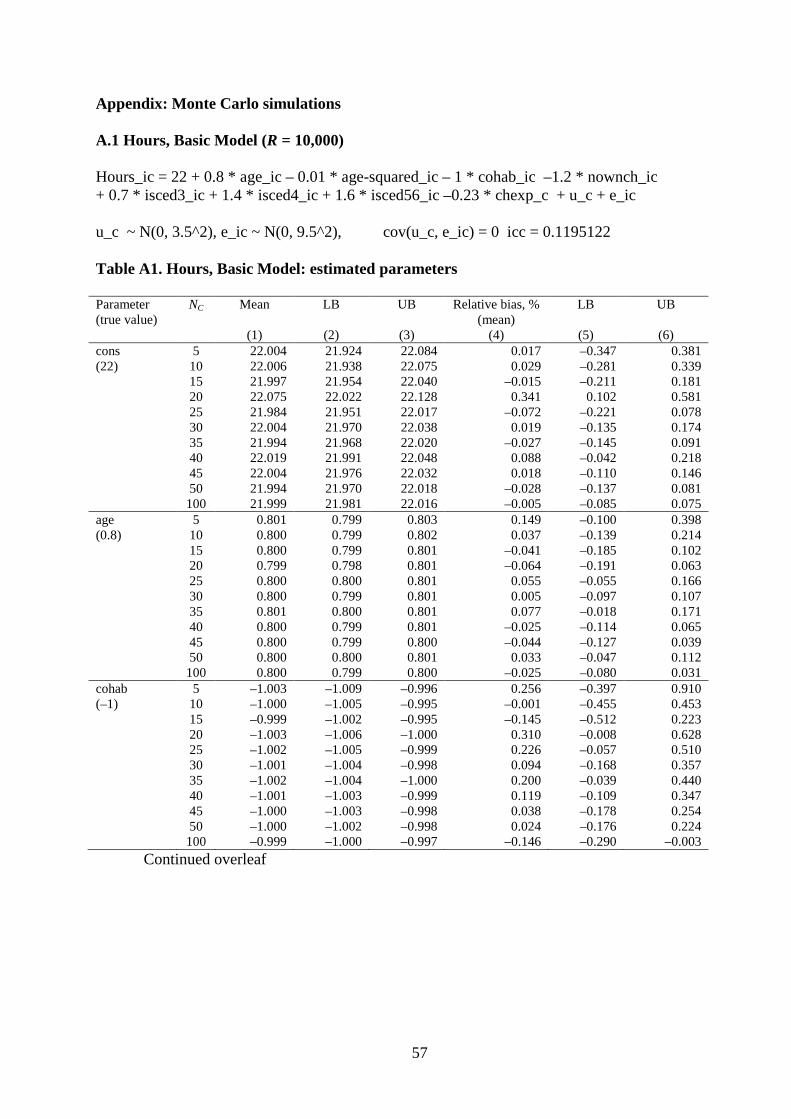
57
Appendix: Monte Carlo simulations A.1 Hours, Basic Model (R = 10,000) Hours_ic = 22 + 0.8 * age_ic – 0.01 * age-squared_ic – 1 * cohab_ic –1.2 * nownch_ic + 0.7 * isced3_ic + 1.4 * isced4_ic + 1.6 * isced56_ic –0.23 * chexp_c + u_c + e_ic u_c ~ N(0, 3.5^2), e_ic ~ N(0, 9.5^2), cov(u_c, e_ic) = 0 icc = 0.1195122 Table A1. Hours, Basic Model: estimated parameters Parameter (true value)
NC Mean LB UB Relative bias, % (mean)
LB UB
(1) (2) (3) (4) (5) (6) cons 5 22.004 21.924 22.084 0.017 –0.347 0.381 (22) 10 22.006 21.938 22.075 0.029 –0.281 0.339 15 21.997 21.954 22.040 –0.015 –0.211 0.181 20 22.075 22.022 22.128 0.341 0.102 0.581 25 21.984 21.951 22.017 –0.072 –0.221 0.078 30 22.004 21.970 22.038 0.019 –0.135 0.174 35 21.994 21.968 22.020 –0.027 –0.145 0.091 40 22.019 21.991 22.048 0.088 –0.042 0.218 45 22.004 21.976 22.032 0.018 –0.110 0.146 50 21.994 21.970 22.018 –0.028 –0.137 0.081 100 21.999 21.981 22.016 –0.005 –0.085 0.075 age 5 0.801 0.799 0.803 0.149 –0.100 0.398 (0.8) 10 0.800 0.799 0.802 0.037 –0.139 0.214 15 0.800 0.799 0.801 –0.041 –0.185 0.102 20 0.799 0.798 0.801 –0.064 –0.191 0.063 25 0.800 0.800 0.801 0.055 –0.055 0.166 30 0.800 0.799 0.801 0.005 –0.097 0.107 35 0.801 0.800 0.801 0.077 –0.018 0.171 40 0.800 0.799 0.801 –0.025 –0.114 0.065 45 0.800 0.799 0.800 –0.044 –0.127 0.039 50 0.800 0.800 0.801 0.033 –0.047 0.112 100 0.800 0.799 0.800 –0.025 –0.080 0.031 cohab 5 –1.003 –1.009 –0.996 0.256 –0.397 0.910 (–1) 10 –1.000 –1.005 –0.995 –0.001 –0.455 0.453 15 –0.999 –1.002 –0.995 –0.145 –0.512 0.223 20 –1.003 –1.006 –1.000 0.310 –0.008 0.628 25 –1.002 –1.005 –0.999 0.226 –0.057 0.510 30 –1.001 –1.004 –0.998 0.094 –0.168 0.357 35 –1.002 –1.004 –1.000 0.200 –0.039 0.440 40 –1.001 –1.003 –0.999 0.119 –0.109 0.347 45 –1.000 –1.003 –0.998 0.038 –0.178 0.254 50 –1.000 –1.002 –0.998 0.024 –0.176 0.224 100 –0.999 –1.000 –0.997 –0.146 –0.290 –0.003
Continued overleaf

58
Table A1 (continued). Hours, Basic Model: estimated parameters Parameter (true value)
NC Mean LB UB Relative bias, % (mean)
LB UB
(1) (2) (3) (4) (5) (6) Nownch 5 –1.202 –1.205 –1.199 0.161 –0.085 0.407 (–1.2) 10 –1.199 –1.201 –1.197 –0.103 –0.275 0.069 15 –1.198 –1.200 –1.197 –0.132 –0.270 0.007 20 –1.201 –1.202 –1.199 0.069 –0.053 0.190 25 –1.199 –1.201 –1.198 –0.046 –0.154 0.062 30 –1.199 –1.200 –1.198 –0.084 –0.183 0.015 35 –1.200 –1.201 –1.199 –0.008 –0.100 0.085 40 –1.200 –1.201 –1.199 –0.021 –0.106 0.063 45 –1.201 –1.202 –1.200 0.068 –0.011 0.146 50 –1.200 –1.201 –1.200 0.041 –0.036 0.118 100 –1.200 –1.201 –1.199 0.011 –0.043 0.066 chexp 5 –0.311 –0.415 –0.206 35.115 –10.298 80.527 (–0.23) 10 –0.235 –0.328 –0.141 2.098 –38.618 42.813 15 –0.197 –0.245 –0.149 –14.360 –35.406 6.686 20 –0.364 –0.460 –0.269 58.421 16.968 99.874 25 –0.223 –0.268 –0.178 –3.206 –22.802 16.389 30 –0.237 –0.284 –0.191 3.247 –17.134 23.628 35 –0.237 –0.268 –0.207 3.191 –10.005 16.387 40 –0.252 –0.286 –0.219 9.775 –4.945 24.496 45 –0.219 –0.261 –0.178 –4.754 –22.776 13.268 50 –0.228 –0.262 –0.194 –0.748 –15.440 13.945 100 –0.227 –0.249 –0.205 –1.261 –10.923 8.402 sig_u 5 3.221 3.194 3.248 –7.967 –8.736 –7.199 (3.5) 10 3.392 3.375 3.408 –3.099 –3.581 –2.616 15 3.447 3.434 3.460 –1.518 –1.900 –1.136 20 3.459 3.448 3.471 –1.165 –1.494 –0.836 25 3.462 3.452 3.473 –1.077 –1.369 –0.785 30 3.469 3.460 3.478 –0.888 –1.151 –0.625 35 3.481 3.472 3.489 –0.555 –0.797 –0.312 40 3.475 3.467 3.483 –0.724 –0.950 –0.497 45 3.478 3.470 3.485 –0.637 –0.846 –0.428 50 3.481 3.474 3.488 –0.533 –0.731 –0.334 100 3.492 3.488 3.497 –0.215 –0.356 –0.073 sig_e 5 9.500 9.498 9.502 0.000 –0.019 0.020 (9.5) 10 9.499 9.498 9.501 –0.008 –0.022 0.006 15 9.499 9.498 9.500 –0.008 –0.020 0.003 20 9.500 9.499 9.501 –0.003 –0.012 0.007 25 9.500 9.499 9.501 –0.003 –0.012 0.005 30 9.500 9.499 9.501 –0.001 –0.009 0.007 35 9.500 9.500 9.501 0.003 –0.005 0.010 40 9.500 9.500 9.501 0.002 –0.005 0.009 45 9.500 9.499 9.501 –0.000 –0.007 0.006 50 9.500 9.499 9.500 –0.001 –0.007 0.005 100 9.500 9.500 9.501 0.001 –0.003 0.005
Continued overleaf
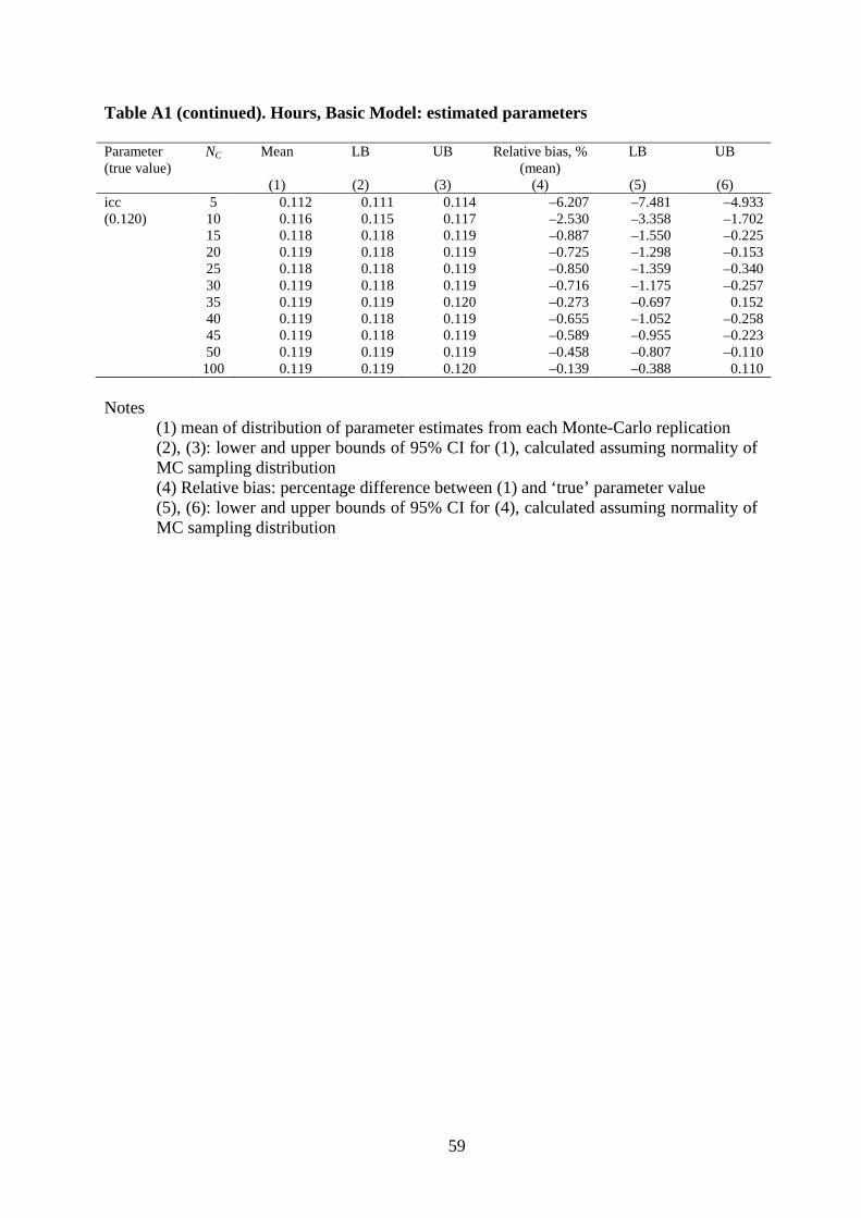
59
Table A1 (continued). Hours, Basic Model: estimated parameters Parameter (true value)
NC Mean LB UB Relative bias, % (mean)
LB UB
(1) (2) (3) (4) (5) (6) icc 5 0.112 0.111 0.114 –6.207 –7.481 –4.933 (0.120) 10 0.116 0.115 0.117 –2.530 –3.358 –1.702 15 0.118 0.118 0.119 –0.887 –1.550 –0.225 20 0.119 0.118 0.119 –0.725 –1.298 –0.153 25 0.118 0.118 0.119 –0.850 –1.359 –0.340 30 0.119 0.118 0.119 –0.716 –1.175 –0.257 35 0.119 0.119 0.120 –0.273 –0.697 0.152 40 0.119 0.118 0.119 –0.655 –1.052 –0.258 45 0.119 0.118 0.119 –0.589 –0.955 –0.223 50 0.119 0.119 0.119 –0.458 –0.807 –0.110 100 0.119 0.119 0.120 –0.139 –0.388 0.110 Notes
(1) mean of distribution of parameter estimates from each Monte-Carlo replication (2), (3): lower and upper bounds of 95% CI for (1), calculated assuming normality of MC sampling distribution (4) Relative bias: percentage difference between (1) and ‘true’ parameter value (5), (6): lower and upper bounds of 95% CI for (4), calculated assuming normality of MC sampling distribution

60
Table A2. Hours, Basic Model: estimated standard errors and non-coverage rates Parameter NC Empirical
SE Analytic
al SE LB UB Relative
difference, %
Non–coverage rate, %
LB UB
(1) (2) (3) (4) (5) (6) (7) (8) cons 5 4.088 3.884 3.861 3.907 –4.981 0.097 0.092 0.103 10 3.479 3.440 3.426 3.454 –1.128 0.070 0.065 0.075 15 2.199 2.182 2.176 2.188 –0.745 0.062 0.057 0.067 20 2.688 2.675 2.667 2.683 –0.472 0.060 0.055 0.065 25 1.678 1.670 1.667 1.674 –0.483 0.056 0.051 0.060 30 1.734 1.712 1.709 1.716 –1.278 0.058 0.053 0.062 35 1.325 1.319 1.317 1.321 –0.457 0.053 0.049 0.057 40 1.454 1.462 1.460 1.465 0.577 0.052 0.048 0.057 45 1.437 1.432 1.430 1.435 –0.283 0.052 0.048 0.057 50 1.221 1.208 1.206 1.210 –1.061 0.056 0.051 0.060 100 0.894 0.886 0.885 0.887 –0.914 0.051 0.047 0.056 age 5 0.101 0.101 0.101 0.101 –0.396 0.051 0.047 0.055 10 0.072 0.072 0.072 0.072 –0.525 0.051 0.046 0.055 15 0.059 0.059 0.059 0.059 –0.045 0.050 0.045 0.054 20 0.052 0.051 0.051 0.051 –1.706 0.055 0.050 0.059 25 0.045 0.046 0.046 0.046 0.926 0.047 0.043 0.051 30 0.042 0.042 0.042 0.042 0.079 0.052 0.048 0.057 35 0.039 0.039 0.039 0.039 0.161 0.052 0.048 0.056 40 0.037 0.036 0.036 0.036 –0.765 0.049 0.045 0.054 45 0.034 0.034 0.034 0.034 0.471 0.048 0.043 0.052 50 0.032 0.032 0.032 0.032 –0.351 0.048 0.044 0.053 100 0.023 0.023 0.023 0.023 0.690 0.049 0.045 0.054 cohab 5 0.333 0.330 0.330 0.330 –1.083 0.052 0.047 0.056 10 0.232 0.229 0.229 0.229 –1.058 0.052 0.047 0.056 15 0.188 0.186 0.186 0.186 –0.600 0.050 0.046 0.054 20 0.162 0.163 0.163 0.163 0.501 0.049 0.045 0.053 25 0.145 0.146 0.146 0.146 0.759 0.049 0.044 0.053 30 0.134 0.134 0.134 0.134 –0.257 0.051 0.047 0.055 35 0.122 0.124 0.124 0.124 1.053 0.048 0.044 0.052 40 0.116 0.116 0.116 0.116 –0.405 0.050 0.046 0.054 45 0.110 0.109 0.109 0.109 –1.066 0.049 0.045 0.054 50 0.102 0.103 0.103 0.103 1.426 0.046 0.042 0.050 100 0.073 0.073 0.073 0.073 –0.448 0.051 0.046 0.055 nownch 5 0.151 0.150 0.150 0.150 –0.344 0.052 0.047 0.056 10 0.105 0.104 0.104 0.104 –0.890 0.055 0.050 0.059 15 0.085 0.085 0.085 0.085 0.586 0.048 0.044 0.052 20 0.074 0.074 0.074 0.074 –0.430 0.051 0.047 0.055 25 0.066 0.066 0.066 0.066 0.279 0.047 0.043 0.051 30 0.061 0.060 0.060 0.060 –0.721 0.052 0.047 0.056 35 0.056 0.056 0.056 0.056 –0.835 0.051 0.047 0.055 40 0.052 0.052 0.052 0.052 0.729 0.050 0.046 0.054 45 0.048 0.049 0.049 0.049 1.858 0.044 0.040 0.048 50 0.047 0.047 0.047 0.047 –0.146 0.051 0.047 0.056 100 0.033 0.033 0.033 0.033 –0.637 0.050 0.046 0.054
Continued overleaf
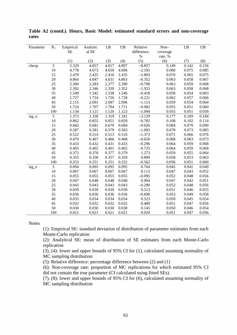
61
Table A2 (contd.). Hours, Basic Model: estimated standard errors and non-coverage rates Parameter NC Empirical
SE Analytic
al SE LB UB Relative
difference, %
Non–coverage rate, %
LB UB
(1) (2) (3) (4) (5) (6) (7) (8) chexp 5 5.329 4.857 4.817 4.897 –8.857 0.149 0.142 0.156 10 4.778 4.673 4.650 4.696 –2.195 0.080 0.075 0.085 15 2.470 2.425 2.416 2.435 –1.803 0.070 0.065 0.075 20 4.864 4.847 4.831 4.863 –0.352 0.063 0.058 0.067 25 2.300 2.283 2.277 2.290 –0.708 0.063 0.059 0.068 30 2.392 2.346 2.339 2.352 –1.923 0.063 0.058 0.068 35 1.549 1.542 1.538 1.546 –0.418 0.058 0.054 0.063 40 1.727 1.724 1.720 1.728 –0.221 0.062 0.057 0.066 45 2.115 2.091 2.087 2.096 –1.113 0.059 0.054 0.064 50 1.724 1.707 1.704 1.711 –0.982 0.055 0.051 0.060 100 1.134 1.121 1.120 1.123 –1.094 0.055 0.051 0.059 sig_u 5 1.373 1.330 1.319 1.341 –3.129 0.177 0.169 0.184 10 0.862 0.855 0.851 0.859 –0.782 0.108 0.102 0.114 15 0.682 0.681 0.679 0.684 –0.026 0.084 0.079 0.090 20 0.587 0.581 0.579 0.583 –1.083 0.078 0.073 0.083 25 0.522 0.514 0.513 0.516 –1.373 0.071 0.066 0.076 30 0.470 0.467 0.466 0.468 –0.650 0.068 0.063 0.073 35 0.433 0.432 0.431 0.433 –0.296 0.064 0.059 0.068 40 0.405 0.402 0.401 0.402 –0.725 0.064 0.059 0.068 45 0.373 0.378 0.377 0.379 1.273 0.059 0.055 0.064 50 0.355 0.358 0.357 0.359 0.899 0.058 0.053 0.063 100 0.253 0.251 0.251 0.252 –0.562 0.056 0.051 0.060 sig_e 5 0.094 0.095 0.095 0.095 0.764 0.045 0.041 0.049 10 0.067 0.067 0.067 0.067 0.113 0.047 0.043 0.052 15 0.055 0.055 0.055 0.055 –0.095 0.052 0.048 0.056 20 0.047 0.048 0.048 0.048 0.904 0.047 0.042 0.051 25 0.043 0.043 0.043 0.043 –0.290 0.052 0.048 0.056 30 0.039 0.039 0.039 0.039 0.513 0.051 0.046 0.055 35 0.036 0.036 0.036 0.036 –0.690 0.053 0.049 0.058 40 0.033 0.034 0.034 0.034 0.323 0.050 0.045 0.054 45 0.032 0.032 0.032 0.032 0.489 0.051 0.047 0.056 50 0.030 0.030 0.030 0.030 0.145 0.050 0.046 0.054 100 0.021 0.021 0.021 0.021 0.020 0.051 0.047 0.056 Notes
(1): Empirical SE: standard deviation of distribution of parameter estimates from each Monte-Carlo replication (2): Analytical SE: mean of distribution of SE estimates from each Monte-Carlo replication (3), (4): lower and upper bounds of 95% CI for (1), calculated assuming normality of MC sampling distribution (5): Relative difference: percentage difference between (2) and (1) (6): Non-coverage rate: proportion of MC replications for which estimated 95% CI did not contain the true parameter (CI calculated using fitted SEs). (7), (8): lower and upper bounds of 95% CI for (6), calculated assuming normality of MC sampling distribution
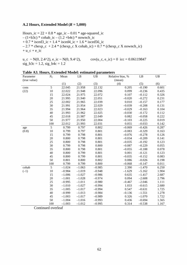
62
A.2 Hours, Extended Model (R = 5,000) Hours_ic = 22 + 0.8 * age_ic – 0.01 * age-squared_ic – (1+b3c) * cohab_ic – (1.2 +b4c) * nownch_ic + 0.7 * isced3_ic + 1.4 * isced4_ic + 1.6 * isced56_ic – 2.7 * chexp_c + 2.4 * (chexp_c X cohab_ic) + 0.7 * (chexp_c X nownch_ic) + u_c + e_ic u_c ~ N(0, 2.4^2), e_ic ~ N(0, 9.4^2), cov(u_c, e_ic) = 0 icc = 0.06119847 sig_b3c = 1.2, sig_b4c = 1.2 Table A3. Hours, Extended Model: estimated parameters Parameter (true value)
NC Mean LB UB Relative bias, % (mean)
LB UB
(1) (2) (3) (4) (5) (6) cons 5 22.045 21.958 22.132 0.205 –0.190 0.601 (22) 10 22.022 21.948 22.096 0.099 –0.236 0.435 15 22.024 21.975 22.072 0.107 –0.112 0.326 20 21.995 21.940 22.051 –0.020 –0.272 0.231 25 22.002 21.965 22.039 0.010 –0.157 0.177 30 21.991 21.954 22.029 –0.039 –0.208 0.131 35 21.994 21.964 22.023 –0.029 –0.163 0.104 40 21.993 21.962 22.025 –0.030 –0.172 0.112 45 22.018 21.987 22.049 0.082 –0.058 0.222 50 21.977 21.950 22.004 –0.103 –0.225 0.019 100 22.012 21.993 22.031 0.055 –0.033 0.142 age 5 0.799 0.797 0.802 –0.069 –0.426 0.287 (0.8) 10 0.799 0.797 0.801 –0.083 –0.329 0.163 15 0.799 0.798 0.801 –0.076 –0.278 0.126 20 0.800 0.798 0.801 –0.034 –0.209 0.141 25 0.800 0.798 0.801 –0.035 –0.192 0.123 30 0.799 0.798 0.800 –0.087 –0.229 0.055 35 0.800 0.798 0.801 –0.055 –0.188 0.078 40 0.800 0.799 0.801 0.001 –0.121 0.123 45 0.800 0.799 0.801 –0.035 –0.152 0.083 50 0.801 0.800 0.802 0.086 –0.026 0.198 100 0.799 0.799 0.800 –0.068 –0.147 0.011 cohab 5 –1.024 –1.063 –0.985 2.390 –1.470 6.250 (–1) 10 –0.984 –1.019 –0.948 –1.629 –5.162 1.904 15 –1.006 –1.027 –0.986 0.635 –1.417 2.687 20 –1.001 –1.028 –0.974 0.094 –2.608 2.796 25 –0.995 –1.011 –0.980 –0.467 –2.046 1.111 30 –1.010 –1.027 –0.994 1.033 –0.615 2.680 35 –1.005 –1.017 –0.994 0.547 –0.631 1.725 40 –0.999 –1.013 –0.984 –0.136 –1.551 1.278 45 –1.003 –1.017 –0.989 0.326 –1.070 1.722 50 –1.004 –1.016 –0.993 0.436 –0.694 1.565 100 –1.003 –1.012 –0.995 0.314 –0.538 1.167
Continued overleaf

63
Table A3 (continued). Hours, Extended Model: estimated parameters Parameter (true value)
NC Mean LB UB Relative bias, % (mean)
LB UB
(1) (2) (3) (4) (5) (6) nownch 5 –1.201 –1.236 –1.166 0.051 –2.866 2.967 (–1.2) 10 –1.182 –1.213 –1.150 –1.516 –4.129 1.096 15 –1.190 –1.209 –1.172 –0.802 –2.334 0.730 20 –1.198 –1.222 –1.173 –0.191 –2.240 1.858 25 –1.197 –1.211 –1.183 –0.254 –1.412 0.904 30 –1.194 –1.209 –1.179 –0.494 –1.756 0.769 35 –1.192 –1.202 –1.181 –0.674 –1.552 0.204 40 –1.203 –1.216 –1.191 0.271 –0.761 1.303 45 –1.194 –1.206 –1.182 –0.491 –1.520 0.539 50 –1.197 –1.207 –1.187 –0.263 –1.114 0.588 100 –1.194 –1.202 –1.187 –0.484 –1.113 0.146 chexp 5 –2.734 –2.836 –2.631 1.244 –2.566 5.053 (– 2.7) 10 –2.719 –2.813 –2.626 0.717 –2.750 4.183 15 –2.716 –2.764 –2.667 0.589 –1.205 2.383 20 –2.681 –2.776 –2.586 –0.691 –4.211 2.829 25 –2.693 –2.739 –2.647 –0.269 –1.981 1.444 30 –2.655 –2.702 –2.608 –1.651 –3.392 0.090 35 –2.687 –2.717 –2.658 –0.463 –1.572 0.645 40 –2.688 –2.722 –2.654 –0.437 –1.688 0.814 45 –2.722 –2.763 –2.682 0.825 –0.682 2.332 50 –2.691 –2.724 –2.658 –0.338 –1.568 0.892 100 –2.706 –2.728 –2.684 0.226 –0.575 1.028 chexpXcohab 5 2.412 2.355 2.468 0.495 –1.863 2.853 (2.4) 10 2.397 2.344 2.450 –0.132 –2.344 2.079 15 2.409 2.382 2.437 0.391 –0.745 1.526 20 2.416 2.363 2.470 0.677 –1.547 2.900 25 2.387 2.361 2.413 –0.552 –1.626 0.522 30 2.410 2.384 2.436 0.420 –0.666 1.505 35 2.412 2.395 2.429 0.504 –0.202 1.210 40 2.402 2.383 2.421 0.100 –0.693 0.893 45 2.411 2.388 2.434 0.468 –0.489 1.426 50 2.413 2.394 2.431 0.532 –0.243 1.307 100 2.409 2.397 2.422 0.380 –0.140 0.900 chexpXnownch 5 0.703 0.650 0.755 0.362 –7.129 7.852 (0.7) 10 0.685 0.638 0.732 –2.138 –8.845 4.568 15 0.688 0.664 0.713 –1.691 –5.170 1.788 20 0.710 0.661 0.758 1.379 –5.508 8.267 25 0.695 0.672 0.717 –0.746 –3.989 2.498 30 0.695 0.672 0.719 –0.656 –4.054 2.742 35 0.691 0.676 0.706 –1.241 –3.386 0.905 40 0.705 0.688 0.721 0.645 –1.752 3.042 45 0.690 0.669 0.710 –1.450 –4.375 1.475 50 0.697 0.680 0.714 –0.449 –2.866 1.968 100 0.695 0.684 0.706 –0.714 –2.303 0.875
Continued overleaf

64
Table A3 (continued). Hours, Extended Model: estimated parameters Parameter (true value)
NC Mean LB UB Relative bias, % (mean)
LB UB
(1) (2) (3) (4) (5) (6) sig_u 5 2.199 2.170 2.227 –8.392 –9.583 –7.202 (2.4) 10 2.318 2.301 2.336 –3.404 –4.125 –2.682 15 2.356 2.342 2.370 –1.828 –2.396 –1.260 20 2.366 2.355 2.378 –1.403 –1.884 –0.922 25 2.373 2.363 2.383 –1.124 –1.551 –0.697 30 2.375 2.366 2.385 –1.037 –1.431 –0.643 35 2.384 2.375 2.392 –0.678 –1.032 –0.324 40 2.388 2.380 2.396 –0.515 –0.850 –0.180 45 2.380 2.373 2.388 –0.815 –1.130 –0.500 50 2.390 2.383 2.398 –0.399 –0.697 –0.101 100 2.391 2.386 2.396 –0.376 –0.582 –0.171 sig_e 5 9.401 9.398 9.404 0.010 –0.018 0.038 (9.4) 10 9.400 9.398 9.402 0.001 –0.019 0.020 15 9.399 9.398 9.401 –0.005 –0.022 0.011 20 9.400 9.399 9.401 –0.000 –0.014 0.014 25 9.400 9.399 9.401 0.001 –0.012 0.013 30 9.400 9.399 9.401 0.001 –0.011 0.012 35 9.399 9.398 9.400 –0.008 –0.019 0.002 40 9.399 9.398 9.400 –0.008 –0.017 0.002 45 9.400 9.399 9.401 –0.001 –0.010 0.008 50 9.400 9.399 9.401 0.001 –0.008 0.009 100 9.399 9.399 9.400 –0.008 –0.015 –0.002 sig_b3c 5 1.024 1.005 1.042 –14.693 –16.245 –13.142 (1.2) 10 1.124 1.112 1.135 –6.355 –7.333 –5.378 15 1.157 1.148 1.166 –3.576 –4.334 –2.819 20 1.168 1.161 1.176 –2.645 –3.276 –2.014 25 1.177 1.170 1.184 –1.918 –2.473 –1.363 30 1.183 1.176 1.189 –1.457 –1.966 –0.947 35 1.182 1.177 1.188 –1.465 –1.924 –1.006 40 1.186 1.181 1.191 –1.152 –1.580 –0.723 45 1.187 1.183 1.192 –1.055 –1.458 –0.653 50 1.189 1.184 1.193 –0.949 –1.330 –0.568 100 1.197 1.194 1.200 –0.265 –0.532 0.002 sig_b4c 5 1.093 1.078 1.107 –14.693 –16.245 –13.142 (1.2) 10 1.156 1.147 1.164 –6.355 –7.333 –5.378 15 1.174 1.167 1.181 –3.576 –4.334 –2.819 20 1.176 1.170 1.181 –2.645 –3.276 –2.014 25 1.189 1.184 1.195 –1.918 –2.473 –1.363 30 1.191 1.187 1.196 –1.457 –1.966 –0.947 35 1.189 1.185 1.193 –1.465 –1.924 –1.006 40 1.191 1.187 1.195 –1.152 –1.580 –0.723 45 1.192 1.188 1.196 –1.055 –1.458 –0.653 50 1.193 1.190 1.197 –0.949 –1.330 –0.568 100 1.198 1.195 1.200 –0.265 –0.532 0.002
Continued overleaf

65
Table A3 (continued). Hours, Extended Model: estimated parameters Icc 5 0.060 0.059 0.061 –2.085 –4.235 0.064 (0.061) 10 0.060 0.059 0.061 –1.476 –2.809 –0.144 15 0.061 0.060 0.062 –0.407 –1.465 0.652 20 0.061 0.060 0.061 –0.475 –1.374 0.424 25 0.061 0.060 0.061 –0.409 –1.205 0.387 30 0.061 0.060 0.061 –0.501 –1.238 0.236 35 0.061 0.061 0.062 –0.093 –0.755 0.569 40 0.061 0.061 0.062 0.090 –0.537 0.717 45 0.061 0.060 0.061 –0.601 –1.189 –0.013 50 0.061 0.061 0.062 0.072 –0.486 0.631 100 0.061 0.061 0.061 –0.300 –0.686 0.086 Notes (1) mean of distribution of parameter estimates from each Monte-Carlo replication (2), (3): lower and upper bounds of 95% CI for (1), calculated assuming normality of MC sampling distribution (4) Relative bias: percentage difference between (1) and ‘true’ parameter value (5), (6): lower and upper bounds of 95% CI for (4), calculated assuming normality of MC sampling distribution
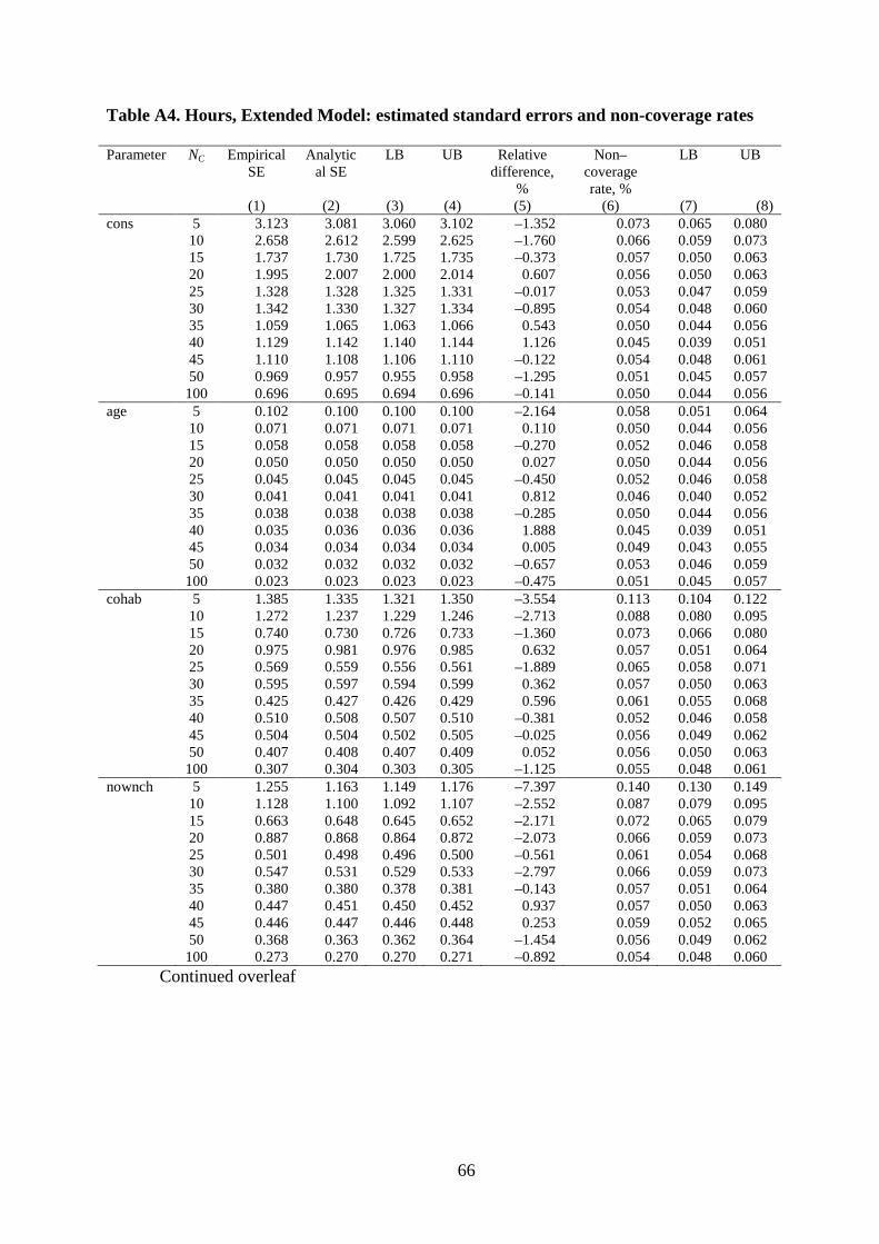
66
Table A4. Hours, Extended Model: estimated standard errors and non-coverage rates Parameter NC Empirical
SE Analytic
al SE LB UB Relative
difference, %
Non–coverage rate, %
LB UB
(1) (2) (3) (4) (5) (6) (7) (8) cons 5 3.123 3.081 3.060 3.102 –1.352 0.073 0.065 0.080 10 2.658 2.612 2.599 2.625 –1.760 0.066 0.059 0.073 15 1.737 1.730 1.725 1.735 –0.373 0.057 0.050 0.063 20 1.995 2.007 2.000 2.014 0.607 0.056 0.050 0.063 25 1.328 1.328 1.325 1.331 –0.017 0.053 0.047 0.059 30 1.342 1.330 1.327 1.334 –0.895 0.054 0.048 0.060 35 1.059 1.065 1.063 1.066 0.543 0.050 0.044 0.056 40 1.129 1.142 1.140 1.144 1.126 0.045 0.039 0.051 45 1.110 1.108 1.106 1.110 –0.122 0.054 0.048 0.061 50 0.969 0.957 0.955 0.958 –1.295 0.051 0.045 0.057 100 0.696 0.695 0.694 0.696 –0.141 0.050 0.044 0.056 age 5 0.102 0.100 0.100 0.100 –2.164 0.058 0.051 0.064 10 0.071 0.071 0.071 0.071 0.110 0.050 0.044 0.056 15 0.058 0.058 0.058 0.058 –0.270 0.052 0.046 0.058 20 0.050 0.050 0.050 0.050 0.027 0.050 0.044 0.056 25 0.045 0.045 0.045 0.045 –0.450 0.052 0.046 0.058 30 0.041 0.041 0.041 0.041 0.812 0.046 0.040 0.052 35 0.038 0.038 0.038 0.038 –0.285 0.050 0.044 0.056 40 0.035 0.036 0.036 0.036 1.888 0.045 0.039 0.051 45 0.034 0.034 0.034 0.034 0.005 0.049 0.043 0.055 50 0.032 0.032 0.032 0.032 –0.657 0.053 0.046 0.059 100 0.023 0.023 0.023 0.023 –0.475 0.051 0.045 0.057 cohab 5 1.385 1.335 1.321 1.350 –3.554 0.113 0.104 0.122 10 1.272 1.237 1.229 1.246 –2.713 0.088 0.080 0.095 15 0.740 0.730 0.726 0.733 –1.360 0.073 0.066 0.080 20 0.975 0.981 0.976 0.985 0.632 0.057 0.051 0.064 25 0.569 0.559 0.556 0.561 –1.889 0.065 0.058 0.071 30 0.595 0.597 0.594 0.599 0.362 0.057 0.050 0.063 35 0.425 0.427 0.426 0.429 0.596 0.061 0.055 0.068 40 0.510 0.508 0.507 0.510 –0.381 0.052 0.046 0.058 45 0.504 0.504 0.502 0.505 –0.025 0.056 0.049 0.062 50 0.407 0.408 0.407 0.409 0.052 0.056 0.050 0.063 100 0.307 0.304 0.303 0.305 –1.125 0.055 0.048 0.061 nownch 5 1.255 1.163 1.149 1.176 –7.397 0.140 0.130 0.149 10 1.128 1.100 1.092 1.107 –2.552 0.087 0.079 0.095 15 0.663 0.648 0.645 0.652 –2.171 0.072 0.065 0.079 20 0.887 0.868 0.864 0.872 –2.073 0.066 0.059 0.073 25 0.501 0.498 0.496 0.500 –0.561 0.061 0.054 0.068 30 0.547 0.531 0.529 0.533 –2.797 0.066 0.059 0.073 35 0.380 0.380 0.378 0.381 –0.143 0.057 0.051 0.064 40 0.447 0.451 0.450 0.452 0.937 0.057 0.050 0.063 45 0.446 0.447 0.446 0.448 0.253 0.059 0.052 0.065 50 0.368 0.363 0.362 0.364 –1.454 0.056 0.049 0.062 100 0.273 0.270 0.270 0.271 –0.892 0.054 0.048 0.060
Continued overleaf
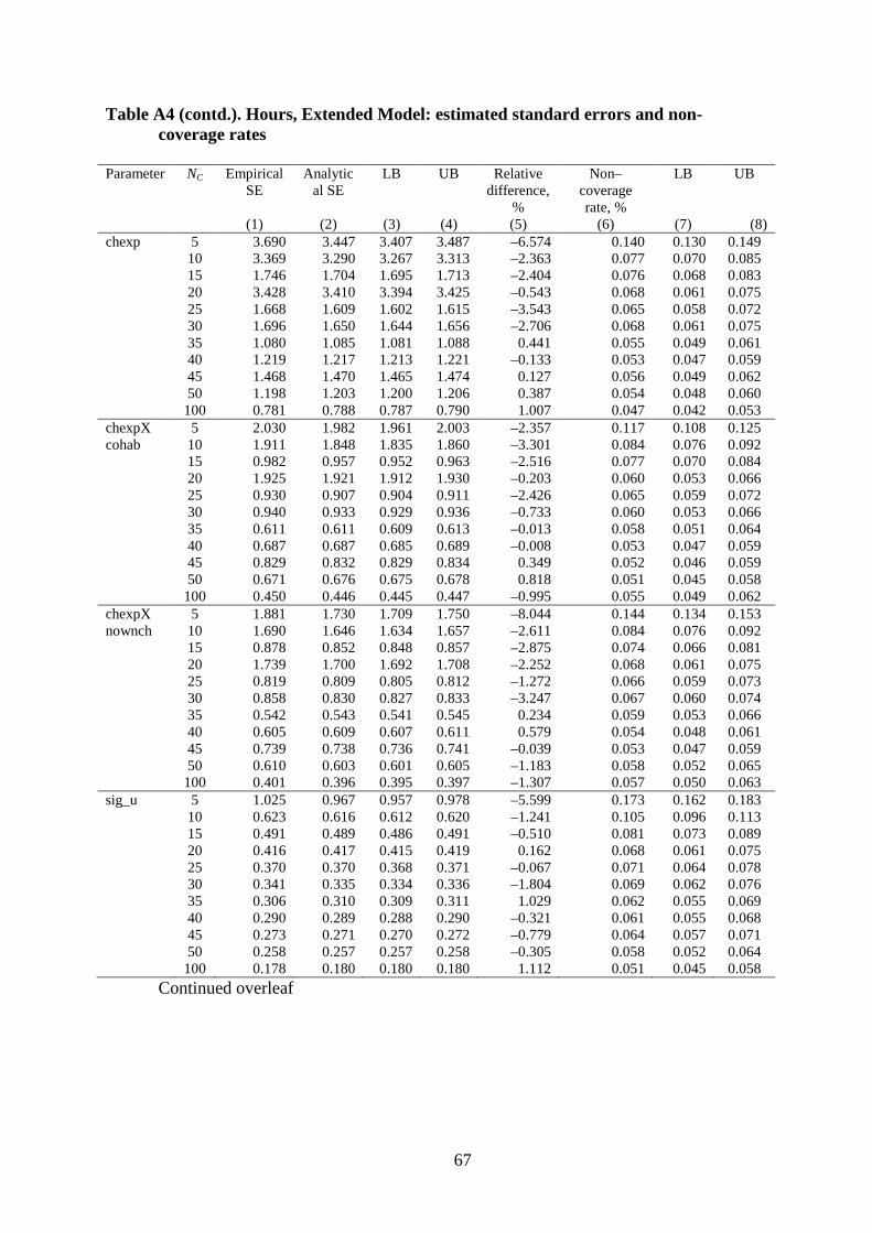
67
Table A4 (contd.). Hours, Extended Model: estimated standard errors and non-coverage rates
Parameter NC Empirical
SE Analytic
al SE LB UB Relative
difference, %
Non–coverage rate, %
LB UB
(1) (2) (3) (4) (5) (6) (7) (8) chexp 5 3.690 3.447 3.407 3.487 –6.574 0.140 0.130 0.149 10 3.369 3.290 3.267 3.313 –2.363 0.077 0.070 0.085 15 1.746 1.704 1.695 1.713 –2.404 0.076 0.068 0.083 20 3.428 3.410 3.394 3.425 –0.543 0.068 0.061 0.075 25 1.668 1.609 1.602 1.615 –3.543 0.065 0.058 0.072 30 1.696 1.650 1.644 1.656 –2.706 0.068 0.061 0.075 35 1.080 1.085 1.081 1.088 0.441 0.055 0.049 0.061 40 1.219 1.217 1.213 1.221 –0.133 0.053 0.047 0.059 45 1.468 1.470 1.465 1.474 0.127 0.056 0.049 0.062 50 1.198 1.203 1.200 1.206 0.387 0.054 0.048 0.060 100 0.781 0.788 0.787 0.790 1.007 0.047 0.042 0.053 chexpX 5 2.030 1.982 1.961 2.003 –2.357 0.117 0.108 0.125 cohab 10 1.911 1.848 1.835 1.860 –3.301 0.084 0.076 0.092 15 0.982 0.957 0.952 0.963 –2.516 0.077 0.070 0.084 20 1.925 1.921 1.912 1.930 –0.203 0.060 0.053 0.066 25 0.930 0.907 0.904 0.911 –2.426 0.065 0.059 0.072 30 0.940 0.933 0.929 0.936 –0.733 0.060 0.053 0.066 35 0.611 0.611 0.609 0.613 –0.013 0.058 0.051 0.064 40 0.687 0.687 0.685 0.689 –0.008 0.053 0.047 0.059 45 0.829 0.832 0.829 0.834 0.349 0.052 0.046 0.059 50 0.671 0.676 0.675 0.678 0.818 0.051 0.045 0.058 100 0.450 0.446 0.445 0.447 –0.995 0.055 0.049 0.062 chexpX 5 1.881 1.730 1.709 1.750 –8.044 0.144 0.134 0.153 nownch 10 1.690 1.646 1.634 1.657 –2.611 0.084 0.076 0.092 15 0.878 0.852 0.848 0.857 –2.875 0.074 0.066 0.081 20 1.739 1.700 1.692 1.708 –2.252 0.068 0.061 0.075 25 0.819 0.809 0.805 0.812 –1.272 0.066 0.059 0.073 30 0.858 0.830 0.827 0.833 –3.247 0.067 0.060 0.074 35 0.542 0.543 0.541 0.545 0.234 0.059 0.053 0.066 40 0.605 0.609 0.607 0.611 0.579 0.054 0.048 0.061 45 0.739 0.738 0.736 0.741 –0.039 0.053 0.047 0.059 50 0.610 0.603 0.601 0.605 –1.183 0.058 0.052 0.065 100 0.401 0.396 0.395 0.397 –1.307 0.057 0.050 0.063 sig_u 5 1.025 0.967 0.957 0.978 –5.599 0.173 0.162 0.183 10 0.623 0.616 0.612 0.620 –1.241 0.105 0.096 0.113 15 0.491 0.489 0.486 0.491 –0.510 0.081 0.073 0.089 20 0.416 0.417 0.415 0.419 0.162 0.068 0.061 0.075 25 0.370 0.370 0.368 0.371 –0.067 0.071 0.064 0.078 30 0.341 0.335 0.334 0.336 –1.804 0.069 0.062 0.076 35 0.306 0.310 0.309 0.311 1.029 0.062 0.055 0.069 40 0.290 0.289 0.288 0.290 –0.321 0.061 0.055 0.068 45 0.273 0.271 0.270 0.272 –0.779 0.064 0.057 0.071 50 0.258 0.257 0.257 0.258 –0.305 0.058 0.052 0.064 100 0.178 0.180 0.180 0.180 1.112 0.051 0.045 0.058
Continued overleaf

68
Table A4 (contd.). Hours, Extended Model: estimated standard errors and non-coverage rates
Parameter NC Empirical
SE Analytic
al SE LB UB Relative
difference, %
Non–coverage rate, %
LB UB
(1) (2) (3) (4) (5) (6) (7) (8) sig_e 5 0.095 0.094 0.094 0.095 –1.127 0.060 0.053 0.066 10 0.067 0.067 0.067 0.067 –0.216 0.049 0.043 0.055 15 0.055 0.054 0.054 0.054 –0.875 0.052 0.046 0.058 20 0.047 0.047 0.047 0.047 –0.594 0.051 0.045 0.058 25 0.042 0.042 0.042 0.042 0.326 0.050 0.044 0.056 30 0.038 0.038 0.038 0.038 0.777 0.048 0.042 0.054 35 0.035 0.036 0.036 0.036 0.560 0.051 0.045 0.057 40 0.033 0.033 0.033 0.033 0.720 0.044 0.039 0.050 45 0.031 0.031 0.031 0.031 1.698 0.044 0.039 0.050 50 0.029 0.030 0.030 0.030 2.348 0.047 0.041 0.052 100 0.021 0.021 0.021 0.021 –1.084 0.053 0.047 0.060 sig_b3c 5 0.668 0.609 0.601 0.618 –8.747 0.151 0.141 0.160 10 0.422 0.402 0.400 0.405 –4.738 0.036 0.031 0.041 15 0.328 0.316 0.315 0.317 –3.541 0.067 0.060 0.074 20 0.273 0.269 0.268 0.270 –1.513 0.065 0.058 0.071 25 0.240 0.237 0.237 0.238 –1.200 0.059 0.052 0.066 30 0.221 0.216 0.215 0.216 –2.215 0.063 0.056 0.070 35 0.199 0.198 0.198 0.199 –0.279 0.053 0.047 0.060 40 0.185 0.185 0.185 0.185 –0.218 0.057 0.051 0.064 45 0.174 0.174 0.173 0.174 –0.405 0.054 0.048 0.060 50 0.165 0.164 0.164 0.165 –0.425 0.054 0.048 0.061 100 0.116 0.115 0.115 0.115 –0.708 0.052 0.045 0.058 sig_b4c 5 0.515 0.492 0.487 0.498 –4.478 0.169 0.159 0.180 10 0.316 0.311 0.309 0.313 –1.654 0.109 0.100 0.117 15 0.253 0.247 0.245 0.248 –2.314 0.091 0.083 0.099 20 0.209 0.210 0.209 0.211 0.553 0.076 0.068 0.083 25 0.190 0.187 0.187 0.188 –1.425 0.069 0.062 0.076 30 0.171 0.170 0.169 0.171 –0.453 0.063 0.056 0.070 35 0.156 0.156 0.156 0.157 0.050 0.065 0.058 0.071 40 0.147 0.146 0.145 0.146 –0.794 0.062 0.055 0.069 45 0.137 0.137 0.137 0.137 0.308 0.062 0.055 0.069 50 0.133 0.130 0.130 0.130 –2.425 0.069 0.062 0.076 100 0.093 0.091 0.091 0.091 –1.537 0.055 0.049 0.062 Notes
(1): Empirical SE: standard deviation of distribution of parameter estimates from each Monte-Carlo replication (2): Analytical SE: mean of distribution of SE estimates from each Monte-Carlo replication (3), (4): lower and upper bounds of 95% CI for (1), calculated assuming normality of MC sampling distribution (5): Relative difference: percentage difference between (2) and (1) (6): Non-coverage rate: proportion of MC replications for which estimated 95% CI did not contain the true parameter (CI calculated using fitted SEs). (7), (8): lower and upper bounds of 95% CI for (6), calculated assuming normality of MC sampling distribution

69
A.3 Participation: basic model (R = 5,000) Logit(participation) = –9.1 + 0.5 * age_ic – 0.006 * age-squared_ic +0.02 * cohab_ic –0. 27 * nownch_ic + 0.7 * isced3_ic + 0.9 * isced4_ic + 1.4 * isced56_ic +0.98 * chexp_c + u_c + e_ic u_c ~ N(0, 0.275^2), e_ic ~ N(0, (_pi^2 / 3)^2), cov(u_c, e_ic) = 0 icc = 0.0224707 Table A5. Participation, Basic Model: estimated parameters Parameter (true value)
NC Mean LB UB Relative bias, % (mean)
LB UB
(1) (2) (3) (4) (5) (6) cons 5 –9.120 –9.133 –9.108 0.221 0.084 0.358 (–9.1) 10 –9.108 –9.120 –9.096 0.086 –0.044 0.215 15 –9.103 –9.111 –9.095 0.034 –0.052 0.120 20 –9.106 –9.113 –9.100 0.071 –0.004 0.147 25 –9.100 –9.106 –9.095 0.005 –0.058 0.067 30 –9.101 –9.106 –9.095 0.006 –0.050 0.062 35 –9.099 –9.104 –9.094 –0.011 –0.067 0.046 40 –9.107 –9.111 –9.102 0.073 0.021 0.126 45 –9.103 –9.107 –9.099 0.031 –0.015 0.078 50 –9.100 –9.104 –9.096 –0.001 –0.045 0.043 100 –9.102 –9.105 –9.100 0.027 –0.005 0.059 age 5 0.501 0.501 0.502 0.233 0.112 0.354 (0.5) 10 0.501 0.500 0.501 0.127 0.042 0.212 15 0.500 0.500 0.501 0.045 –0.025 0.115 20 0.500 0.500 0.500 0.036 –0.024 0.095 25 0.500 0.500 0.500 0.019 –0.034 0.072 30 0.500 0.500 0.500 0.028 –0.022 0.078 35 0.500 0.500 0.500 –0.001 –0.048 0.045 40 0.500 0.500 0.500 0.050 0.008 0.092 45 0.500 0.500 0.500 0.034 –0.006 0.074 50 0.500 0.500 0.500 0.001 –0.037 0.039 100 0.500 0.500 0.500 0.012 –0.015 0.039 cohab 5 0.018 0.015 0.020 –11.903 –24.547 0.741 (0.02) 10 0.019 0.017 0.020 –7.215 –15.725 1.295 15 0.019 0.017 0.020 –6.394 –13.722 0.934 20 0.019 0.018 0.021 –2.641 –8.855 3.573 25 0.019 0.018 0.020 –4.031 –9.636 1.574 30 0.020 0.018 0.021 –2.357 –7.518 2.804 35 0.020 0.019 0.021 2.143 –2.562 6.848 40 0.020 0.019 0.020 –1.942 –6.286 2.403 45 0.020 0.020 0.021 1.871 –2.213 5.956 50 0.020 0.019 0.021 –0.952 –4.906 3.001 100 0.020 0.020 0.021 1.439 –1.328 4.205 nownch 5 –0.270 –0.271 –0.269 –0.008 –0.466 0.451 (–0.27) 10 –0.270 –0.271 –0.269 –0.099 –0.412 0.215 15 –0.269 –0.270 –0.269 –0.217 –0.480 0.046 20 –0.270 –0.271 –0.270 0.088 –0.142 0.317 25 –0.270 –0.270 –0.269 –0.182 –0.384 0.021 30 –0.270 –0.270 –0.269 –0.095 –0.283 0.093 35 –0.270 –0.270 –0.269 –0.116 –0.287 0.055 40 –0.270 –0.271 –0.270 0.077 –0.080 0.234 45 –0.270 –0.271 –0.270 0.076 –0.075 0.228 50 –0.270 –0.270 –0.270 –0.020 –0.166 0.125 100 –0.270 –0.270 –0.270 –0.031 –0.131 0.068
Continued overleaf
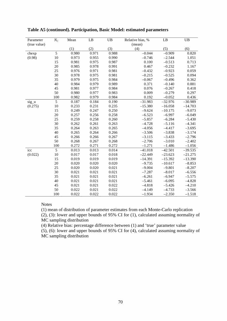
70
Table A5 (continued). Participation, Basic Model: estimated parameters Parameter (true value)
NC Mean LB UB Relative bias, % (mean)
LB UB
(1) (2) (3) (4) (5) (6) chexp 5 0.980 0.971 0.988 –0.044 –0.909 0.820 (0.98) 10 0.973 0.955 0.990 –0.746 –2.544 1.051 15 0.981 0.975 0.987 0.100 –0.513 0.713 20 0.985 0.978 0.991 0.467 –0.232 1.167 25 0.976 0.971 0.981 –0.432 –0.923 0.059 30 0.978 0.975 0.981 –0.215 –0.525 0.094 35 0.979 0.975 0.984 –0.067 –0.496 0.362 40 0.984 0.979 0.989 0.371 –0.140 0.881 45 0.981 0.977 0.984 0.076 –0.267 0.418 50 0.980 0.977 0.983 0.009 –0.279 0.297 100 0.982 0.979 0.984 0.192 –0.052 0.436 sig_u 5 0.187 0.184 0.190 –31.983 –32.976 –30.989 (0.275) 10 0.233 0.231 0.235 –15.380 –16.058 –14.703 15 0.249 0.247 0.250 –9.624 –10.175 –9.073 20 0.257 0.256 0.258 –6.523 –6.997 –6.049 25 0.259 0.258 0.260 –5.857 –6.284 –5.430 30 0.262 0.261 0.263 –4.728 –5.116 –4.341 35 0.264 0.263 0.265 –4.056 –4.417 –3.695 40 0.265 0.264 0.266 –3.506 –3.838 –3.174 45 0.266 0.266 0.267 –3.115 –3.433 –2.796 50 0.268 0.267 0.268 –2.706 –3.010 –2.402 100 0.272 0.271 0.272 –1.271 –1.486 –1.056 icc 5 0.013 0.013 0.014 –41.018 –42.501 –39.535 (0.022) 10 0.017 0.017 0.018 –22.449 –23.623 –21.275 15 0.019 0.019 0.019 –14.391 –15.392 –13.390 20 0.020 0.020 0.020 –9.735 –10.617 –8.853 25 0.020 0.020 0.021 –9.004 –9.801 –8.207 30 0.021 0.021 0.021 –7.287 –8.017 –6.556 35 0.021 0.021 0.021 –6.261 –6.947 –5.575 40 0.021 0.021 0.021 –5.461 –6.095 –4.828 45 0.021 0.021 0.022 –4.818 –5.426 –4.210 50 0.022 0.021 0.022 –4.149 –4.733 –3.566 100 0.022 0.022 0.022 –1.934 –2.350 –1.518
Notes (1) mean of distribution of parameter estimates from each Monte-Carlo replication (2), (3): lower and upper bounds of 95% CI for (1), calculated assuming normality of MC sampling distribution (4) Relative bias: percentage difference between (1) and ‘true’ parameter value (5), (6): lower and upper bounds of 95% CI for (4), calculated assuming normality of MC sampling distribution

71
Table A6. Participation, Basic Model: estimated standard errors and non-coverage rates
Parameter NC Empirical
SE Analytic
al SE LB UB Relative
difference, %
Non–coverage rate, %
LB UB
(1) (2) (3) (4) (5) (6) (7) (8) cons 5 0.449 0.427 0.426 0.428 –4.968 0.064 0.057 0.071 10 0.425 0.387 0.386 0.388 –8.985 0.081 0.073 0.089 15 0.282 0.271 0.271 0.272 –3.709 0.055 0.048 0.061 20 0.248 0.244 0.243 0.244 –1.847 0.056 0.050 0.063 25 0.207 0.205 0.205 0.205 –0.841 0.053 0.047 0.059 30 0.184 0.183 0.183 0.183 –0.441 0.050 0.044 0.056 35 0.185 0.180 0.179 0.180 –3.166 0.057 0.051 0.064 40 0.172 0.172 0.172 0.172 –0.190 0.050 0.044 0.056 45 0.153 0.152 0.151 0.152 –0.794 0.052 0.045 0.058 50 0.145 0.144 0.144 0.145 –0.218 0.050 0.044 0.056 100 0.105 0.104 0.104 0.104 –1.251 0.053 0.046 0.059 age 5 0.022 0.022 0.022 0.022 –0.706 0.051 0.045 0.057 10 0.015 0.015 0.015 0.015 –1.717 0.058 0.051 0.064 15 0.013 0.013 0.013 0.013 0.288 0.049 0.043 0.055 20 0.011 0.011 0.011 0.011 0.991 0.049 0.043 0.055 25 0.010 0.010 0.010 0.010 1.344 0.047 0.041 0.053 30 0.009 0.009 0.009 0.009 0.373 0.049 0.043 0.055 35 0.008 0.008 0.008 0.008 –1.411 0.051 0.045 0.057 40 0.008 0.008 0.008 0.008 0.104 0.051 0.045 0.058 45 0.007 0.007 0.007 0.007 –0.331 0.047 0.041 0.053 50 0.007 0.007 0.007 0.007 0.070 0.053 0.047 0.059 100 0.005 0.005 0.005 0.005 –0.691 0.052 0.046 0.058 cohab 5 0.091 0.090 0.090 0.090 –1.085 0.056 0.049 0.062 10 0.061 0.062 0.062 0.062 0.868 0.045 0.039 0.051 15 0.053 0.052 0.052 0.052 –1.621 0.058 0.051 0.064 20 0.045 0.045 0.045 0.045 –0.481 0.051 0.045 0.057 25 0.040 0.040 0.040 0.040 –0.952 0.055 0.049 0.061 30 0.037 0.037 0.037 0.037 –0.359 0.046 0.040 0.051 35 0.034 0.034 0.034 0.034 0.045 0.050 0.044 0.056 40 0.031 0.031 0.031 0.031 –0.545 0.050 0.044 0.056 45 0.029 0.030 0.030 0.030 0.229 0.053 0.047 0.060 50 0.029 0.028 0.028 0.028 –0.189 0.049 0.043 0.055 100 0.020 0.020 0.020 0.020 –0.346 0.048 0.042 0.054 nownch 5 0.045 0.045 0.044 0.045 –0.295 0.048 0.042 0.054 10 0.031 0.030 0.030 0.030 –0.500 0.049 0.043 0.055 15 0.026 0.026 0.026 0.026 1.219 0.048 0.042 0.054 20 0.022 0.022 0.022 0.022 –1.543 0.051 0.045 0.057 25 0.020 0.020 0.020 0.020 0.107 0.050 0.044 0.056 30 0.018 0.018 0.018 0.018 0.365 0.047 0.041 0.053 35 0.017 0.017 0.017 0.017 0.223 0.050 0.044 0.056 40 0.015 0.015 0.015 0.015 0.578 0.048 0.042 0.054 45 0.015 0.015 0.015 0.015 –1.508 0.053 0.047 0.059 50 0.014 0.014 0.014 0.014 –1.034 0.054 0.048 0.060 100 0.010 0.010 0.010 0.010 1.005 0.044 0.038 0.049
Continued overleaf
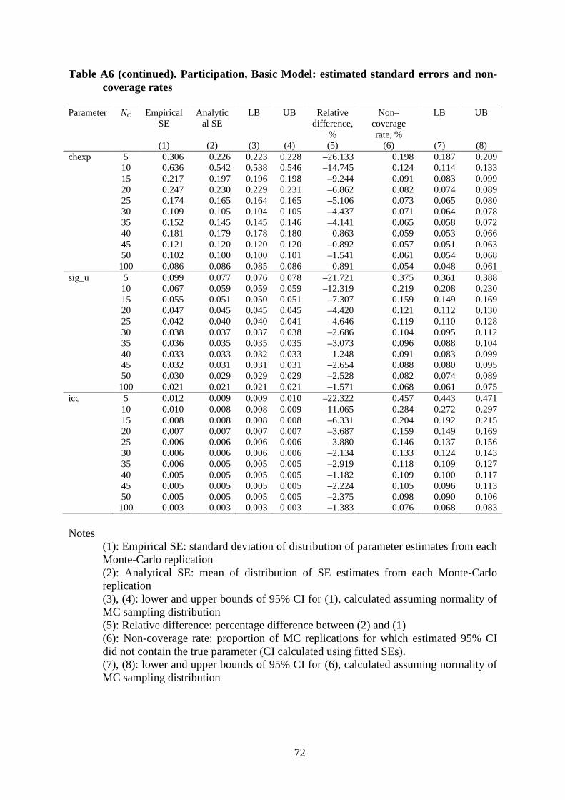
72
Table A6 (continued). Participation, Basic Model: estimated standard errors and non-coverage rates
Parameter NC Empirical
SE Analytic
al SE LB UB Relative
difference, %
Non–coverage rate, %
LB UB
(1) (2) (3) (4) (5) (6) (7) (8) chexp 5 0.306 0.226 0.223 0.228 –26.133 0.198 0.187 0.209 10 0.636 0.542 0.538 0.546 –14.745 0.124 0.114 0.133 15 0.217 0.197 0.196 0.198 –9.244 0.091 0.083 0.099 20 0.247 0.230 0.229 0.231 –6.862 0.082 0.074 0.089 25 0.174 0.165 0.164 0.165 –5.106 0.073 0.065 0.080 30 0.109 0.105 0.104 0.105 –4.437 0.071 0.064 0.078 35 0.152 0.145 0.145 0.146 –4.141 0.065 0.058 0.072 40 0.181 0.179 0.178 0.180 –0.863 0.059 0.053 0.066 45 0.121 0.120 0.120 0.120 –0.892 0.057 0.051 0.063 50 0.102 0.100 0.100 0.101 –1.541 0.061 0.054 0.068 100 0.086 0.086 0.085 0.086 –0.891 0.054 0.048 0.061 sig_u 5 0.099 0.077 0.076 0.078 –21.721 0.375 0.361 0.388 10 0.067 0.059 0.059 0.059 –12.319 0.219 0.208 0.230 15 0.055 0.051 0.050 0.051 –7.307 0.159 0.149 0.169 20 0.047 0.045 0.045 0.045 –4.420 0.121 0.112 0.130 25 0.042 0.040 0.040 0.041 –4.646 0.119 0.110 0.128 30 0.038 0.037 0.037 0.038 –2.686 0.104 0.095 0.112 35 0.036 0.035 0.035 0.035 –3.073 0.096 0.088 0.104 40 0.033 0.033 0.032 0.033 –1.248 0.091 0.083 0.099 45 0.032 0.031 0.031 0.031 –2.654 0.088 0.080 0.095 50 0.030 0.029 0.029 0.029 –2.528 0.082 0.074 0.089 100 0.021 0.021 0.021 0.021 –1.571 0.068 0.061 0.075 icc 5 0.012 0.009 0.009 0.010 –22.322 0.457 0.443 0.471 10 0.010 0.008 0.008 0.009 –11.065 0.284 0.272 0.297 15 0.008 0.008 0.008 0.008 –6.331 0.204 0.192 0.215 20 0.007 0.007 0.007 0.007 –3.687 0.159 0.149 0.169 25 0.006 0.006 0.006 0.006 –3.880 0.146 0.137 0.156 30 0.006 0.006 0.006 0.006 –2.134 0.133 0.124 0.143 35 0.006 0.005 0.005 0.005 –2.919 0.118 0.109 0.127 40 0.005 0.005 0.005 0.005 –1.182 0.109 0.100 0.117 45 0.005 0.005 0.005 0.005 –2.224 0.105 0.096 0.113 50 0.005 0.005 0.005 0.005 –2.375 0.098 0.090 0.106 100 0.003 0.003 0.003 0.003 –1.383 0.076 0.068 0.083 Notes
(1): Empirical SE: standard deviation of distribution of parameter estimates from each Monte-Carlo replication (2): Analytical SE: mean of distribution of SE estimates from each Monte-Carlo replication (3), (4): lower and upper bounds of 95% CI for (1), calculated assuming normality of MC sampling distribution (5): Relative difference: percentage difference between (2) and (1) (6): Non-coverage rate: proportion of MC replications for which estimated 95% CI did not contain the true parameter (CI calculated using fitted SEs). (7), (8): lower and upper bounds of 95% CI for (6), calculated assuming normality of MC sampling distribution

73
A.4 Participation, Extended Model (R = 1,000) Logit(participation) = –9.1 + 0.5 * age_ic – 0.006 * age-squared_ic + (0.02 + b3c)* cohab_ic –(0. 27+b4c) * nownch_ic + 0.7 * isced3_ic + 0.9 * isced4_ic + 1.4 * isced56_ic +0.7 * chexp_c + 0.6 * (chexp_c X cohab_ic) – 0.1 * (chexp_c X nownch_ic)+ u_c + e_ic u_c ~ N(0, 0.38^2), e_ic ~ N(0, (_pi^2 / 3)^2), cov(u_c, e_ic) = 0 icc = 0.0420468 sig_b3c = 0.25, sig_b4c = 0.13 Table A7. Participation, Extended Model: estimated parameters Parameter (true value)
NC Mean LB UB Relative bias, % (mean)
LB UB
(1) (2) (3) (4) (5) (6) cons 5 –9.123 –9.154 –9.092 0.251 –0.090 0.591 (–9.1) 10 –9.121 –9.154 –9.088 0.229 –0.136 0.594 15 –9.095 –9.116 –9.075 –0.050 –0.271 0.172 20 –9.103 –9.122 –9.084 0.034 –0.171 0.239 25 –9.104 –9.119 –9.089 0.046 –0.118 0.210 30 –9.107 –9.120 –9.094 0.076 –0.063 0.215 35 –9.111 –9.124 –9.098 0.116 –0.027 0.259 40 –9.110 –9.123 –9.098 0.114 –0.025 0.253 45 –9.108 –9.119 –9.097 0.086 –0.035 0.207 50 –9.102 –9.113 –9.091 0.023 –0.096 0.142 100 –9.093 –9.101 –9.085 –0.078 –0.163 0.007 age 5 0.500 0.499 0.502 0.073 –0.197 0.344 (0.5) 10 0.501 0.500 0.502 0.123 –0.065 0.311 15 0.500 0.499 0.501 0.029 –0.135 0.194 20 0.500 0.500 0.501 0.082 –0.054 0.218 25 0.500 0.500 0.501 0.059 –0.062 0.179 30 0.501 0.500 0.501 0.119 0.010 0.228 35 0.500 0.500 0.501 0.008 –0.094 0.110 40 0.501 0.500 0.501 0.127 0.034 0.219 45 0.500 0.500 0.501 0.082 –0.009 0.173 50 0.500 0.500 0.500 –0.005 –0.092 0.082 100 0.500 0.500 0.500 –0.001 –0.062 0.059 cohab 5 0.023 0.007 0.039 17.346 –62.683 97.375 (0.02) 10 0.003 –0.019 0.024 –85.267 –192.878 22.345 15 0.013 0.002 0.025 –34.069 –90.803 22.665 20 0.017 0.007 0.028 –12.500 –65.711 40.710 25 0.021 0.013 0.029 6.628 –33.061 46.317 30 0.018 0.012 0.025 –8.579 –40.080 22.922 35 0.018 0.010 0.025 –12.385 –48.637 23.866 40 0.025 0.017 0.032 23.028 –14.476 60.533 45 0.017 0.011 0.023 –14.908 –45.281 15.464 50 0.022 0.017 0.028 12.279 –16.730 41.288 100 0.019 0.014 0.023 –7.037 –27.730 13.656
Continued overleaf

74
Table A7 (continued). Participation, Extended Model: estimated parameters Parameter (true value)
NC Mean LB UB Relative bias, % (mean)
LB UB
(1) (2) (3) (4) (5) (6) nownch 5 –0.271 –0.279 –0.263 0.324 –2.753 3.402 (–0. 27) 10 –0.266 –0.276 –0.255 –1.582 –5.552 2.388 15 –0.266 –0.272 –0.261 –1.358 –3.507 0.791 20 –0.273 –0.279 –0.267 1.022 –1.114 3.158 25 –0.270 –0.274 –0.266 0.100 –1.407 1.607 30 –0.271 –0.275 –0.268 0.510 –0.702 1.721 35 –0.269 –0.273 –0.266 –0.279 –1.646 1.088 40 –0.270 –0.274 –0.266 –0.061 –1.467 1.344 45 –0.274 –0.277 –0.270 1.297 0.185 2.408 50 –0.270 –0.273 –0.267 0.042 –1.063 1.147 100 –0.271 –0.273 –0.269 0.483 –0.309 1.276 chexp 5 0.720 0.694 0.747 2.916 –0.895 6.728 (0.7) 10 0.726 0.671 0.781 3.747 –4.133 11.627 15 0.692 0.673 0.710 –1.191 –3.872 1.489 20 0.701 0.679 0.722 0.076 –2.943 3.094 25 0.699 0.684 0.714 –0.191 –2.345 1.963 30 0.701 0.691 0.710 0.100 –1.277 1.476 35 0.711 0.698 0.724 1.563 –0.277 3.404 40 0.700 0.684 0.716 –0.060 –2.341 2.221 45 0.701 0.690 0.713 0.210 –1.439 1.859 50 0.697 0.685 0.708 –0.476 –2.114 1.161 100 0.690 0.682 0.699 –1.360 –2.533 –0.187 chexpXcohab 5 0.599 0.578 0.621 –0.131 –3.722 3.461 (0.6) 10 0.643 0.601 0.685 7.173 0.231 14.116 15 0.614 0.599 0.629 2.319 –0.235 4.873 20 0.602 0.585 0.619 0.337 –2.445 3.120 25 0.602 0.590 0.614 0.300 –1.687 2.288 30 0.601 0.594 0.609 0.245 –1.065 1.554 35 0.603 0.592 0.613 0.448 –1.279 2.175 40 0.594 0.581 0.606 –1.060 –3.202 1.081 45 0.603 0.594 0.613 0.577 –0.950 2.104 50 0.596 0.588 0.605 –0.597 –2.037 0.842 100 0.604 0.597 0.610 0.622 –0.453 1.697 chexpXnownch 5 –0.097 –0.108 –0.086 –2.724 –13.826 8.377 (–0.1) 10 –0.112 –0.133 –0.091 12.201 –8.852 33.255 15 –0.103 –0.110 –0.095 2.554 –4.947 10.054 20 –0.097 –0.106 –0.088 –2.983 –11.917 5.951 25 –0.101 –0.107 –0.095 0.693 –5.466 6.852 30 –0.100 –0.104 –0.096 0.003 –4.108 4.114 35 –0.101 –0.106 –0.095 0.527 –4.586 5.640 40 –0.099 –0.105 –0.093 –0.955 –7.391 5.481 45 –0.096 –0.100 –0.091 –4.328 –8.957 0.301 50 –0.099 –0.104 –0.095 –0.530 –5.053 3.994 100 –0.099 –0.102 –0.095 –1.296 –4.583 1.992
Continued overleaf

75
Table A7 (continued). Participation, Extended Model: estimated parameters Parameter (true value)
NC Mean LB UB Relative bias, % (mean)
LB UB
(1) (2) (3) (4) (5) (6) sig_u 5 0.249 0.240 0.258 –34.412 –36.768 –32.056 (0.38) 10 0.329 0.323 0.336 –13.291 –14.895 –11.688 15 0.344 0.339 0.349 –9.369 –10.667 –8.072 20 0.356 0.352 0.360 –6.354 –7.452 –5.256 25 0.357 0.354 0.361 –5.945 –6.919 –4.972 30 0.364 0.361 0.368 –4.206 –5.128 –3.285 35 0.364 0.361 0.368 –4.100 –4.931 –3.269 40 0.366 0.363 0.369 –3.593 –4.361 –2.826 45 0.369 0.366 0.372 –2.931 –3.635 –2.227 50 0.372 0.369 0.374 –2.165 –2.881 –1.448 100 0.375 0.373 0.377 –1.359 –1.848 –0.869 sig_b3c 5 0.129 0.121 0.136 –48.589 –51.639 –45.540 (0.25) 10 0.194 0.188 0.200 –22.291 –24.656 –19.926 15 0.215 0.211 0.220 –13.845 –15.728 –11.962 20 0.223 0.219 0.227 –10.863 –12.524 –9.203 25 0.228 0.225 0.232 –8.649 –10.060 –7.238 30 0.235 0.232 0.238 –6.100 –7.363 –4.836 35 0.234 0.232 0.237 –6.249 –7.391 –5.107 40 0.240 0.238 0.243 –3.852 –4.925 –2.778 45 0.239 0.236 0.241 –4.579 –5.605 –3.553 50 0.241 0.239 0.244 –3.519 –4.460 –2.579 100 0.245 0.243 0.247 –1.981 –2.650 –1.312 sig_b4c 5 0.074 0.070 0.078 –43.315 –46.451 –40.179 (0.13) 10 0.102 0.100 0.105 –21.195 –23.432 –18.959 15 0.113 0.110 0.115 –13.387 –15.162 –11.613 20 0.116 0.114 0.118 –10.688 –12.222 –9.153 25 0.119 0.118 0.121 –8.112 –9.469 –6.755 30 0.122 0.120 0.123 –6.440 –7.650 –5.231 35 0.122 0.121 0.124 –5.874 –6.926 –4.823 40 0.123 0.122 0.124 –5.427 –6.420 –4.435 45 0.126 0.124 0.127 –3.456 –4.391 –2.522 50 0.125 0.124 0.126 –3.898 –4.810 –2.987 100 0.127 0.127 0.128 –2.042 –2.681 –1.404 icc 5 0.024 0.023 0.025 –42.905 –46.294 –39.516 (0.042) 10 0.034 0.033 0.035 –18.394 –21.144 –15.643 15 0.036 0.035 0.037 –13.588 –15.868 –11.308 20 0.038 0.037 0.039 –9.282 –11.300 –7.264 25 0.038 0.037 0.039 –9.087 –10.870 –7.304 30 0.039 0.039 0.040 –6.127 –7.841 –4.412 35 0.039 0.039 0.040 –6.264 –7.814 –4.714 40 0.040 0.039 0.040 –5.542 –6.980 –4.104 45 0.040 0.040 0.041 –4.506 –5.826 –3.186 50 0.041 0.040 0.041 –3.037 –4.388 –1.686 100 0.041 0.041 0.042 –2.089 –3.020 –1.159 Notes (1) mean of distribution of parameter estimates from each Monte-Carlo replication (2), (3): lower and upper bounds of 95% CI for (1), calculated assuming normality of MC sampling distribution (4) Relative bias: percentage difference between (1) and ‘true’ parameter value (5), (6): lower and upper bounds of 95% CI for (4), calculated assuming normality of MC sampling distribution
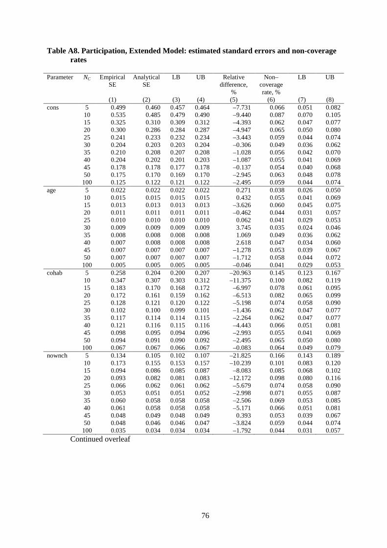
76
Table A8. Participation, Extended Model: estimated standard errors and non-coverage rates
Parameter NC Empirical
SE Analytical
SE LB UB Relative
difference, %
Non–coverage rate, %
LB UB
(1) (2) (3) (4) (5) (6) (7) (8) cons 5 0.499 0.460 0.457 0.464 –7.731 0.066 0.051 0.082 10 0.535 0.485 0.479 0.490 –9.440 0.087 0.070 0.105 15 0.325 0.310 0.309 0.312 –4.393 0.062 0.047 0.077 20 0.300 0.286 0.284 0.287 –4.947 0.065 0.050 0.080 25 0.241 0.233 0.232 0.234 –3.443 0.059 0.044 0.074 30 0.204 0.203 0.203 0.204 –0.306 0.049 0.036 0.062 35 0.210 0.208 0.207 0.208 –1.028 0.056 0.042 0.070 40 0.204 0.202 0.201 0.203 –1.087 0.055 0.041 0.069 45 0.178 0.178 0.177 0.178 –0.137 0.054 0.040 0.068 50 0.175 0.170 0.169 0.170 –2.945 0.063 0.048 0.078 100 0.125 0.122 0.121 0.122 –2.495 0.059 0.044 0.074 age 5 0.022 0.022 0.022 0.022 0.271 0.038 0.026 0.050 10 0.015 0.015 0.015 0.015 0.432 0.055 0.041 0.069 15 0.013 0.013 0.013 0.013 –3.626 0.060 0.045 0.075 20 0.011 0.011 0.011 0.011 –0.462 0.044 0.031 0.057 25 0.010 0.010 0.010 0.010 0.062 0.041 0.029 0.053 30 0.009 0.009 0.009 0.009 3.745 0.035 0.024 0.046 35 0.008 0.008 0.008 0.008 1.069 0.049 0.036 0.062 40 0.007 0.008 0.008 0.008 2.618 0.047 0.034 0.060 45 0.007 0.007 0.007 0.007 –1.278 0.053 0.039 0.067 50 0.007 0.007 0.007 0.007 –1.712 0.058 0.044 0.072 100 0.005 0.005 0.005 0.005 –0.046 0.041 0.029 0.053 cohab 5 0.258 0.204 0.200 0.207 –20.963 0.145 0.123 0.167 10 0.347 0.307 0.303 0.312 –11.375 0.100 0.082 0.119 15 0.183 0.170 0.168 0.172 –6.997 0.078 0.061 0.095 20 0.172 0.161 0.159 0.162 –6.513 0.082 0.065 0.099 25 0.128 0.121 0.120 0.122 –5.198 0.074 0.058 0.090 30 0.102 0.100 0.099 0.101 –1.436 0.062 0.047 0.077 35 0.117 0.114 0.114 0.115 –2.264 0.062 0.047 0.077 40 0.121 0.116 0.115 0.116 –4.443 0.066 0.051 0.081 45 0.098 0.095 0.094 0.096 –2.993 0.055 0.041 0.069 50 0.094 0.091 0.090 0.092 –2.495 0.065 0.050 0.080 100 0.067 0.067 0.066 0.067 –0.083 0.064 0.049 0.079 nownch 5 0.134 0.105 0.102 0.107 –21.825 0.166 0.143 0.189 10 0.173 0.155 0.153 0.157 –10.239 0.101 0.083 0.120 15 0.094 0.086 0.085 0.087 –8.083 0.085 0.068 0.102 20 0.093 0.082 0.081 0.083 –12.172 0.098 0.080 0.116 25 0.066 0.062 0.061 0.062 –5.679 0.074 0.058 0.090 30 0.053 0.051 0.051 0.052 –2.998 0.071 0.055 0.087 35 0.060 0.058 0.058 0.058 –2.506 0.069 0.053 0.085 40 0.061 0.058 0.058 0.058 –5.171 0.066 0.051 0.081 45 0.048 0.049 0.048 0.049 0.393 0.053 0.039 0.067 50 0.048 0.046 0.046 0.047 –3.824 0.059 0.044 0.074 100 0.035 0.034 0.034 0.034 –1.792 0.044 0.031 0.057
Continued overleaf

77
Table A8 (continued). Participation, Extended Model: estimated standard errors and non-coverage rates
Parameter NC Empirical
SE Analytical
SE LB UB Relative
difference, %
Non–coverage rate, %
LB UB
(1) (2) (3) (4) (5) (6) (7) (8) chexp 5 0.429 0.313 0.305 0.321 –27.154 0.226 0.200 0.252 10 0.888 0.785 0.773 0.797 –11.650 0.118 0.098 0.139 15 0.303 0.275 0.272 0.278 –9.152 0.092 0.074 0.110 20 0.341 0.325 0.321 0.328 –4.743 0.083 0.066 0.100 25 0.243 0.231 0.229 0.233 –5.203 0.069 0.053 0.085 30 0.155 0.146 0.144 0.147 –6.332 0.066 0.051 0.081 35 0.208 0.204 0.202 0.205 –1.978 0.070 0.054 0.086 40 0.258 0.252 0.250 0.253 –2.354 0.061 0.046 0.076 45 0.186 0.184 0.182 0.185 –1.290 0.064 0.049 0.079 50 0.185 0.170 0.167 0.173 –8.007 0.066 0.051 0.081 100 0.132 0.130 0.129 0.131 –1.912 0.066 0.051 0.081 chexpX 5 0.347 0.277 0.272 0.282 –20.113 0.144 0.122 0.166 Cohab 10 0.671 0.604 0.595 0.613 –9.956 0.105 0.086 0.125 15 0.247 0.228 0.226 0.231 –7.648 0.077 0.060 0.094 20 0.269 0.251 0.249 0.254 –6.639 0.086 0.069 0.103 25 0.192 0.184 0.182 0.185 –4.514 0.068 0.052 0.084 30 0.127 0.123 0.122 0.124 –2.746 0.066 0.051 0.081 35 0.167 0.161 0.160 0.163 –3.445 0.053 0.039 0.067 40 0.207 0.197 0.196 0.198 –4.945 0.070 0.054 0.086 45 0.148 0.145 0.144 0.146 –1.841 0.054 0.040 0.068 50 0.139 0.135 0.133 0.137 –2.977 0.053 0.039 0.067 100 0.104 0.102 0.102 0.103 –1.559 0.053 0.039 0.067 chexpX 5 0.179 0.142 0.140 0.145 –20.298 0.156 0.133 0.178 nownch 10 0.339 0.305 0.300 0.309 –10.078 0.104 0.085 0.123 15 0.121 0.115 0.113 0.116 –5.254 0.068 0.052 0.084 20 0.144 0.129 0.127 0.130 –10.807 0.098 0.080 0.116 25 0.099 0.094 0.093 0.095 –5.196 0.076 0.060 0.092 30 0.066 0.064 0.063 0.064 –4.159 0.074 0.058 0.090 35 0.082 0.082 0.082 0.083 –0.394 0.058 0.044 0.072 40 0.104 0.099 0.098 0.100 –4.628 0.062 0.047 0.077 45 0.075 0.074 0.074 0.075 –0.584 0.057 0.043 0.071 50 0.073 0.069 0.068 0.070 –5.970 0.065 0.050 0.080 100 0.053 0.052 0.052 0.053 –1.646 0.066 0.051 0.081 sig_u 5 0.144 0.108 0.106 0.110 –24.934 0.390 0.360 0.420 10 0.098 0.085 0.084 0.086 –13.293 0.198 0.173 0.223 15 0.080 0.072 0.071 0.072 –9.849 0.154 0.132 0.176 20 0.067 0.063 0.063 0.064 –5.874 0.124 0.104 0.144 25 0.060 0.057 0.056 0.057 –4.806 0.118 0.098 0.138 30 0.056 0.053 0.052 0.053 –6.520 0.107 0.088 0.126 35 0.051 0.049 0.049 0.049 –4.099 0.089 0.071 0.107 40 0.047 0.046 0.046 0.046 –2.579 0.084 0.067 0.101 45 0.043 0.043 0.043 0.044 0.647 0.071 0.055 0.087 50 0.044 0.042 0.041 0.042 –5.456 0.092 0.074 0.110 100 0.030 0.030 0.029 0.030 –1.655 0.063 0.048 0.078
Continued overleaf

78
Table A8 (continued). Participation, Extended Model: estimated standard errors and non-coverage rates
Parameter NC Empirical
SE Analytical
SE LB UB Relative
difference, %
Non–coverage rate, %
LB UB
(1) (2) (3) (4) (5) (6) (7) (8) sig_b3c 5 0.123 0.133 0.128 0.137 8.287 0.231 0.205 0.257 10 0.095 0.090 0.088 0.093 –5.233 0.050 0.037 0.064 15 0.076 0.072 0.070 0.073 –5.656 0.049 0.036 0.062 20 0.067 0.060 0.060 0.061 –10.047 0.081 0.064 0.098 25 0.057 0.053 0.053 0.054 –6.158 0.086 0.069 0.103 30 0.051 0.049 0.049 0.049 –3.890 0.068 0.052 0.084 35 0.046 0.045 0.045 0.045 –2.778 0.083 0.066 0.100 40 0.043 0.042 0.041 0.042 –4.000 0.070 0.054 0.086 45 0.041 0.039 0.039 0.039 –5.299 0.083 0.066 0.100 50 0.038 0.037 0.037 0.038 –1.407 0.067 0.051 0.083 100 0.027 0.026 0.026 0.026 –2.364 0.064 0.049 0.079 sig_b4c 5 0.066 0.070 0.067 0.073 6.843 0.192 0.167 0.216 10 0.047 0.044 0.043 0.045 –5.468 0.056 0.042 0.071 15 0.037 0.036 0.035 0.036 –4.441 0.079 0.062 0.096 20 0.032 0.030 0.029 0.031 –6.362 0.109 0.090 0.128 25 0.028 0.027 0.026 0.027 –6.687 0.093 0.075 0.111 30 0.025 0.024 0.024 0.025 –3.683 0.070 0.054 0.086 35 0.022 0.022 0.022 0.022 1.054 0.069 0.053 0.085 40 0.021 0.021 0.021 0.021 –0.760 0.072 0.056 0.088 45 0.020 0.020 0.020 0.020 0.129 0.062 0.047 0.077 50 0.019 0.019 0.019 0.019 –2.060 0.075 0.059 0.091 100 0.013 0.013 0.013 0.013 –1.381 0.062 0.047 0.077 icchat 5 0.023 0.017 0.016 0.018 –26.398 0.468 0.437 0.499 10 0.019 0.017 0.016 0.017 –11.112 0.250 0.223 0.277 15 0.015 0.014 0.014 0.015 –7.591 0.202 0.177 0.227 20 0.014 0.013 0.013 0.013 –5.616 0.156 0.133 0.179 25 0.012 0.012 0.011 0.012 –4.185 0.141 0.119 0.163 30 0.012 0.011 0.011 0.011 –6.176 0.137 0.116 0.158 35 0.011 0.010 0.010 0.010 –4.038 0.107 0.088 0.126 40 0.010 0.009 0.009 0.010 –2.686 0.100 0.081 0.119 45 0.009 0.009 0.009 0.009 0.930 0.081 0.064 0.098 50 0.009 0.009 0.009 0.009 –5.118 0.107 0.088 0.126 100 0.006 0.006 0.006 0.006 –1.719 0.074 0.058 0.090 Notes
(1): Empirical SE: standard deviation of distribution of parameter estimates from each Monte–Carlo replication (2): Analytical SE: mean of distribution of SE estimates from each Monte–Carlo replication (3), (4): lower and upper bounds of 95% CI for (1), calculated assuming normality of MC sampling distribution (5): Relative difference: percentage difference between (2) and (1) (6): Non-coverage rate: proportion of MC replications for which estimated 95% CI did not contain the true parameter (CI calculated using fitted SEs). (7), (8): lower and upper bounds of 95% CI for (6), calculated assuming normality of MC sampling distribution