Department of Economics

Working Paper No. 164

Regional integration, international

liberalization and the dynamics of

industrial agglomeration

Pasquale Commendatore Ingrid Kubin

Carmelo Petraglia

Iryna Sushko

January 2014

brought to you by COREView metadata, citation and similar papers at core.ac.uk

provided by Elektronische Publikationen der Wirtschaftsuniversität Wien

Regional integration, international liberalisationand the dynamics of industrial agglomeration

Pasquale CommendatoreUniversity of Naples Federico II

Ingrid KubinVienna University of Economics and Business Administration

Carmelo PetragliaUniversity of Basilicata

Iryna SushkoInstitute of Mathematics, National Academy of Sciences of Ukraine

November 21, 2013

Abstract

This paper presents a 3-Region footloose-entrepreneur new economicgeography model. Two symmetric regions are part of an economicallyintegrated area (the Union), while the third region represents an outsidetrade partner. We explore how the spatial allocation of industrial pro-duction and employment within the Union is a¤ected by changes in twoaspects of trade liberalisation: regional integration and globalisation. Ourmain contribution pertains to the analysis of the local and global dynamicsof the speci�ed factor mobility process. We show that signi�cant parame-ter ranges exist for which asymmetric distribution of economic activitiesis one of the possible long-run outcomes. This is a remarkable resultwithin the NEG literature. We then analyse the impact of internationaltrade liberalisation on the dynamics of agglomeration conditional on theendowments of skilled and unskilled labour of the ouside region.

Keywords: Industrial agglomeration, New Economic Geography, foot-loose entrepreneurs, local and global dynamics, bifurcation scenarios

JEL classi�cation: C62, F12, F2, R12.

1 Introduction

New Economic Geography (NEG) models do not typically account for the pres-ence of regions other than the ones involved in the economic integration process.Nevertheless, a vast body of empirical evidence reveals the ongoing long-term

1

parallel trends of increasing regional integration and globalisation. The EU is apart of this phenomenon: on the one hand, within-EU integration has becomemore important over the last decades and, on the other, the EU as a whole hasgained greater exposure to the world economy (Foster et al. [2013]).The analytic structure of NEG models is intrinsically complex, therefore

many NEG models are actually con�ned to the analysis of two regions, aiming topredict the impact of stronger integration on industrial agglomeration in a giveneconomically integrated area (e.g., EU regions). However, the understanding ofagglomeration and dispersion forces stemming from stronger exposure of theintegrated area to the rest of the world (e.g., EU integration into the worldeconomy) requires a more general set up including (at least) an �outside�region.Scholars dealing with 3-region NEG models � see, among others, Paluzie

[2001]; Krugman and Elizondo [1996]; Brülhart et al. [2004] �typically explorehow the spatial distribution of economic activities in a given home country isa¤ected by international trade liberalisation. On the other hand, as pointed outby Behrens [2011], a large part of this literature underplays the role of regionalintegration. That is, one relevant aspect of economic integration �globalisation� is studied, while the second one � regional integration � is left out of thepicture.Inspired by the case of the EU, the main aim of this paper is to explore how

the spatial allocation of industrial production and employment within an eco-nomically integrated area (the Union) is a¤ected by changes in both aspects oftrade liberalisation: regional integration and globalisation. Our main objectiveis to study the e¤ects of higher integration within the Union (reduced internaltransport costs), and those due to higher economic integration of the Union as awhole with the rest of the World (reduced external transport costs). This is the�rst contribution of the paper. Furthermore, motivated by the changing pictureof the main trade partners of the EU, we study the impact of both aspects ofintegration under alternative assumptions on the industrialisation level of theUnion�s trade partners. In particular, we will show that integration with lessindustrialised regions will make agglomeration of industrial activity within theUnion less likely. In addition, we also analyse the e¤ects of international inte-gration under alternative assumptions about the size of the outside region. Formany parameter values, trade liberalisation ultimately leads to agglomerationof economic activity with the Union. However, the pattern of the transition toagglomeration depends upon the size of the outside region. When integratingwith a small outsider region, catastrophic agglomeration will be observed; in-stead when integrating with a large outsider country, the transition path to fullagglomeration will be smooth.We depart from the existing multi-region NEG models in three ways. In

contrast with most previous contributions, we assume that unskilled workersare immobile both domestically and internationally. This assumption makes ourmodel closer to the reality of the EU where labour mobility plays a relativelyunimportant role as compared to other economically integrated areas such asthe US (Gáková and Dijkstra [2008]). On the other hand, we will maintainthat the interregional mobile factor is human / knowledge capital embodied

2

in skilled workers and entrepreneurs (Forslid and Ottaviano [2003]). A secondimportant departure is the speci�cation of our model in discrete time. Thisrepresents an easy way to account for delays in the dynamic process (that areobviously involved in �rm relocations). Finally, we try to �ll a relevant gap inthe NEG literature: the lack of explicit dynamic analysis. This is a particularlyrelevant issue as many core results of the NEG depend on the properties ofdynamic processes, such as multiple equilibria, change in stability properties, thenature of the basins of attraction. We carefully analyse the emerging bifurcationscenarios �detecting a typical sequence �and show that coexistence of equilibriais much more pervasive than in standard NEG models. We show that in somecases � due to the complex structure of the basins of attraction � it is evenimpossible to predict the long-run spatial distribution of economic activity.The remainder of the paper is structured as follows. Section 2 provides some

stylised facts on the case of EU which inspired our work and reviews the main�ndings of the literature most related to our contribution. Section 3 presentsthe general framework of the model including the de�nition of short-run andlong-run equilibria. Section 4 describes the equilibrium properties of the model.Section 5 presents results on local and global dynamics of the model. Section 6concludes.

2 Stylised facts and Related Literature

The departure point for our analysis are three stylised facts:

� Trade barriers among European regions have been lowered by the longterm process of EU integration;

� globalisation has produced greater exposure of the EU to the world econ-omy, leading to higher dependency of the Union (and of each MemberState) on �nal demand outside the EU;

� the deeper integration into the world economy of the EU is currently char-acterised by an increasing weight of big, less industrialised trade partners.

The strenghtening of the EU internal integration is a well documented fact.Figure 1 outlines the evolution of economic integration within the EU from 1957to 2001 based on the composite index developed by Dorrucci et al. [2002]. Thisis a numerical composite index based on scores attributed to each single eventof European integration grouped according to Balassa [1961] �ve main stagesof regional integration: a) Free Trade Area (FTA) where internal tari¤s andquotas are abolished for imports from area members; b) Customs Union (CU):a FTA setting up tari¤s and quotas for trade with non-members; c) CommonMarket (CM): a CU where restrictions on factor movements as well as non-tari¤ barriers to trade are abolished; d) Economic Union (EUN): a CM with

3

a signi�cant degree of co-ordination of national policies and harmonisation ofrelevant domestic laws; and (e) Total Economic Integration (TEI), an EUN withall relevant economic policies conducted at a supra-national level.Looking at Figure 1 one can identify three sub-periods. The �rst period goes

from March 1957 (Treaty of Rome) to July 1968 (completion of the CU) andis characterised by faster integration as, by the end of this period, more thanhalf of the overall institutional integration process had been already completed.In the late 1960s, the EU was indeed much more than a CU, having alreadysome genuine characteristics of subsequent Balassa stages. The second period(between the early 1970s and the mid-1980s) is characterised by sluggish inte-gration, with the noteworthy exception of the European Monetary System startin March 1979. In the third period, the creation of the CM and the MonetaryUnion has led to considerable acceleration in regional integration. As a result,the EU/euro area in early 2000s could already be classi�ed somewhere betweenan EUN and a TEI. The 2004 and 2007 EU enlargements to Eastern countrieshas then pushed this process forward.

Figure 1: The Index of EU Economic Integration (1957-2001); Source: Dorrucciet al. [2002]; Notes: The index is de�ned for the EU-6 founding members;Highest score possible for regional integration: 100; 1957 = 0.

Turning to the second stylised fact, note that the EU launched in 2006 itsnew �Global Europe� strategy aiming at further integrating the EU into theworld economy (see for a discussion of the institutional progress, Kleimann

4

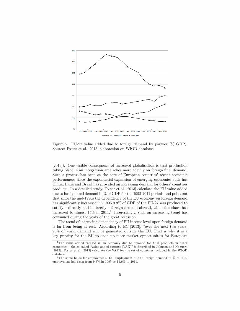
Figure 2: EU-27 value added due to foreign demand by partner (% GDP).Source: Foster et al. [2013] elaboration on WIOD database

[2013]). One visible consequence of increased globalisation is that productiontaking place in an integration area relies more heavily on foreign �nal demand.Such a process has been at the core of European countries� recent economicperformances since the exponential expansion of emerging economies such hasChina, India and Brazil has provided an increasing demand for others�countriesproducts. In a detailed study, Foster et al. [2013] calculate the EU value addeddue to foreign �nal demand in % of GDP for the 1995-2011 period1 and point outthat since the mid-1990s the dependency of the EU economy on foreign demandhas signi�cantly increased: in 1995 9.9% of GDP of the EU-27 was produced tosatisfy �directly and indirectly �foreign demand abroad, while this share hasincreased to almost 15% in 2011.2 Interestingly, such an increasing trend hascontinued during the years of the great recession.The trend of increasing dependency of EU income level upon foreign demand

is far from being at rest. According to EC [2013], �over the next two years,90% of world demand will be generated outside the EU. That is why it is akey priority for the EU to open up more market opportunities for European

1The value added created in an economy due to demand for �nal products in othereconomies �the so-called �value added exports (VAX)� is described in Johnson and Noguera[2012]. Foster et al. [2013] calculate the VAX for the set of countries included in the WIODdatabase.

2The same holds for employment. EU employment due to foreign demand in % of totalemployment has risen from 9.3% in 1995 to 11.6% in 2011.

5

business by negotiating new Free Trade Agreements with key countries. If wewere to complete all our current free trade talks tomorrow, we would add 2.2%to the EU�s GDP or e275 billion. This is equivalent of adding a country asbig as Austria or Denmark to the EU economy. In terms of employment, theseagreements could generate 2.2 million new jobs or additional 1% of the EU totalworkforce.�3

Turning to our third stylised fact, note that the �gures for the valued addeddue to foreign demand disaggregated by trading partners, reveal striking regionaldisparities (see Figure 2): China�s share increased from 3.3% in 1995 to more11.1% in 2011 at the expense of Japan (8.1% in 1995 and 3.4% in 2011) and theUS (24.5% in 1995 compared to 18.4% in 2011).A recent OECD study (Woo [2012]) shows that these changes in the trad-

ing partners involve also a change in the technology level. Based on growthaccounting, (Woo [2012], p15) uncovers a considerable technology gap betweenChina and the US and Japan respectively. Labour productivity in China asmeasured by output per worker is 16% of that of US workers in 2007 and thetotal factor productivity level as a measure of technology (or overall e¢ ciency)in China are 25% of the US counterpart. Japan�s labour productivity (totalfactor productivity) is 69% (54%) of the respective US value.These facts imply relevant research questions to be answered in multi-region

NEG models. That is, how are both agglomeration and dispersion forces thatdrive agglomeration of economic activities a¤ected once deeper integration withinthe union and within the world economy is considered? And how relevant arethe size and the industrialisation level of the trade partners?So far a small strand of literature has developed 3-region models within the

NEG literature. Inspired by the debate on the role of protectionist policies inthe development of a pattern of striking regional inequalities during the Span-ish industrialisation process, Paluzie [2001] proposes a standard core peripherymodel accommodating for the presence of a third region. She considers a worldeconomy consisting of two domestic regions and one external economy, withlabour being mobile only domestically. In line with Krugman [1991], the cen-tripetal forces that produce agglomerations are represented by the interactionof economies of scales, market size and transport costs, while centrifugal forcesthat tend to weaken agglomerations are the pull of a dispersed rural market.The main result in the model is that a reduction in the external trade coststrengthens the agglomerative forces in the home country with two regions. Inother words, external trade liberalisation is expected to increase regional in-equalities in the country that opens up to trade. Similar results are put forwardby Alonso-Villar [2001], and Monfort and Nicolini [2000].Krugman and Elizondo [1996], obtain the opposite result, in the same con-

text of a model with three regions, two domestic and one external, where thedomestic dispersion force is due to land rent and commuting costs and it is thusexogenous and independent of trade costs. The authors study the impact of

3For an overview of the most important forthcoming and on-going free trade negotiationssee EC [2013].

6

trade liberalisation on the distribution of economic activities within the homecountry and conclude that opening up external trade favours dispersion of eco-nomic activity between the two internal regions. It is claimed in the paperthat such a result explains the rise of large metropolis in developing countries(Mexico City is the case discussed by the authors) and its progressive loss ofimportance after the implementation of trade liberalisation policies.Brülhart et al. [2004] and Crozet and Soubeyran [2004] introduce more ge-

ographical structure into the analysis, as they assume that one of the homeregions is a border region, i.e. that it has lower transport cost with respect tothe outside region than the other home region. Also in these frameworks, a re-duction of the international transport cost favours agglomeration in the 2-regionhome country.Brülhart et al. [2004] present a footloose entrepreneur model � a 3-region

version of P�üger [2004] �where two of the three regions are relatively inte-grated. The aim of the authors is to track how the economies of these tworegions are a¤ected by an opening towards the third region. The real worldcase that motivate this work is the 2004 EU enlargement, which integrated tenCentral and Eastern European countries (the third region) fully into the EU�sinternal market. The research question is then linked to the implications forthe distribution of economic activities in the incumbent EU countries of the im-proved access to and from the third region. In the model, the production of themanufactured good requires one unit of human capital and a variable amountof labour. Human capital is mobile between the two regions in one country butimmobile with respect to the third region. The sectorial location is determinedendogenously through the interplay of agglomeration and dispersion forces. Ex-ternal market opening has a bearing on several spatial forces. Forces relatedto better access to foreign export markets and cheaper imports enhance thelocational attraction of the border region. Conversely, forces related to importcompetition from foreign �rms enhance the locational attraction of the interiorregion. The interplay of these forces in the non-linear setup of the model canlead to a variety of equilibria. The main results are such that the range ofparameter values, for which domestic manufacturing agglomerates in only oneregion, increases as external trade costs fall. The same result obtains if �givenconstant external trade costs �the foreign country gets bigger, i.e., the largerthe outside economy, ceteris paribus, the greater the probability that domesticmanufacturing agglomerates in one region. Hence, the size of the third regionmatters for the results.Wang and Zheng [2013] notice that in most developing economies, like China,

a country includes a gate region and the hinterland, where the gate region hasbetter access to overseas markets and the hinterland has a greater share ofunskilled workers. Hence, they extend the standard framework of Krugman[1991] by assuming that domestic regions are asymmetrical in terms of their sizesand accessibilities. They obtain two key results. First, when international tradeliberalisation continues but domestic regions remain poorly integrated, the gateregion experiences a change from partial to full agglomeration. Second, when acountry is closed to global markets, regional integration makes the hinterland

7

attractive to a greater share of manufacturing �rms. However, when a countryis extremely open to global markets, full agglomeration of manufacturing �rmsoccurs in the gate region.With the exception of Brülhart et al. [2004] and Crozet and Soubeyran

[2004], in the above mentioned contributions, labour mobility is the dynamicprocess bringing agglomeration about. This is the case of Krugman and Elizondo[1996] for Mexico, Paluzie [2001] for Spain andWang and Zheng [2013] for China.In all these cases labour mobility is plausible whereas this is not the case forthe EU.As shown by Gáková and Dijkstra [2008], labour mobility between the re-

gions of the EU at NUTS 2 level is relatively low. This seems to be a commonfeature in the EU as it applies to both the old and the new Member States, irre-spective of their economic development or the openness of their labour market.In particular, the analysis provided by Gáková and Dijkstra [2008] shows thatthe share of working age residents moving in another EU region represents, onaverage, less than 1% of the EU�s working age population (vs 2% in the US).4 Asmigration in Europe is rather weak, as far as the EU is concerned, the mobilityof unskilled workers does not really appear to play the role of an adjustmentprocess to wage di¤erential among countries (Siebert [1997]; Obstfeld and Peri[1998]; Puga [2002]). On the other hand, �rm mobility has been achieving anincreasing role since the EU enlargement to the Eastern European countriesfrom the mid-1990s.The contributions whose main results have been summarised earlier in this

section share the common feature of addressing only one part of the issuesat hand as they only analyse the e¤ects of a closer integration of the homeeconomy with the rest of the world, independently of the transportation costswithin the home economy itself. Nevertheless, con�ning our attention to theEU, two parallel trends have been taking place in the last decades � gainingmomentum with the EU enlargement to the Eastern European countries �andprovide the �rst two stylised facts for our theoretical framework. Moreover,the higher importance gained by China at the expenses of the US provides amotivation for studying the e¤ects of globalisation conditional upon the size andthe output composition of the external commercial partners.

3 General framework

In this section we present a variant of the 3-region NEG model developed inForslid and Ottaviano [2003] where the mobile factor is human / knowledgecapital, embodied in skilled workers or, equivalently in their framework, �entre-preneurs�. This is particularly convenient in a multiregional framework for tworeasons. First, the assumption of mobile skilled workers / entrepreneurs implies

4The analysis presented in this paper is based on the average share of the working ageresidents in 2005-2006 who had changed their region of residence during the previous year.

8

analytical tractability and it matches the empirical evidence (esp. for Europe)according to which skilled workers / entrepreneurial undertakings are typicallymore mobile than less specialised labour (Forslid and Ottaviano [2003], p. 230).Di¤erently from Forslid and Ottaviano [2003], we envisage a situation in whichthe entrepreneurs mobility could be limited by various types of barriers (for ex-ample: national, cultural, language and legal barriers), even stronger than thoseconstraining the unskilled workforce migration. Speci�cally, in our framework,entrepreneurial migration occurs only within an economically integrated area (aUnion composed of two regions) and no factor movements take place betweenthe Union and the rest of the World.

3.1 Basic assumptions

We consider an economy composed of 3 regions (r = 1; 2; 3). Regions 1 and2 are part of an economically integrated area (the Union); region 3 insteadrepresents an outside trade partner. There are two sectors, agriculture (A) andmanufacturing (M). There is a unique homogeneous agricultural good producedunder perfect competition, while manufacturing involves n di¤erentiated vari-eties produced by monopolistically competitive �rms. Unskilled workers (L)and entrepreneurs (E) are endowed with (unskilled) labour and human capi-tal, respectively. Workers are immobile (but can be reallocated across sectors),whereas entrepreneurs can migrate only between region 1 and 2, i.e. within theUnion. We assume that there is not factor mobility between the Union andregion 3.L is the amount of unskilled labour in the overall economy and �r is the share

of labour located in region r(= 1; 2; 3); it follows that �rL is the endowment ofunskilled workers of region r. With immobile unskilled workers and a constantand equal to one wage rate (see below), �rL can also be interpreted as the size oflocal demand (�r representing its share) which is not a¤ected by entrepreneurialmigration. When regions 1 and 2 are symmetric, we have that �1 = �2 = � and�3 = 1 � 2�. Moreover, E represents the overall number of entrepreneurs inthe economy and eE the number of entrepreneurs that are free to move betweenregions 1 and 2. We denote by en = eE

E the corresponding share. Consequently,E = E � eE represents the number of immobile entrepreneurs located in region3 and 1� en = E

E = 1�eEE is the corresponding share.

3.2 Consumers�preferences

The three regions are homogeneous in terms of tastes. Individual (entrepreneuror unskilled worker) preferences are expressed by a two-tier utility function. Theupper-tier concerns the choice between agricultural and manufactured goodsaccording to the following Cobb-Douglas utility function:

U = C�MC1��A

9

where CA is the consumption of the agricultural good. The lower-tier concernsthe consumption of the composite of manufactured varieties, CM , given thefollowing CES function:

CM =

nXi=1

c��1�

i

! ���1

where ci represents the quantity consumed of the variety i, with i = 1; :::; n; �the constant elasticity of substitution / taste for variety: the closer � to 1, thegreater is consumer�s taste for variety, with � > 1; and � and 1�� represent theincome shares devoted to the manufactured varieties and to the homogeneousagricultural good, respectively, with 0 < � < 1.

The budget constraint of an individual resident in region r is

NXi=1

epici + pACA = y (1)

where pA is the price of the homogeneous agricultural good; epi is the priceof variety i inclusive of transport costs and y is the income of the individualagent (unskilled worker or entrepreneur).

3.3 Production

The A sector is characterised by perfect competition and constant returns toscale. Production of 1 unit of output requires only � unit of L; without lossof generality, we set � = 1. Moreover, we assume that none of the regions hasenough labour to engage exclusively in the production of the agricultural good,that is, the so-called �non-full-specialisation condition�holds.TheM sector is (Dixit-Stiglitz) monopolistically competitive. It is modelled

according to a few basic characteristics: identical �rms produce di¤erentiatedgoods / varieties with the same production technology involving a �xed compo-nent (one entrepreneur), and a variable component (unskilled workers), with �units of L required for each unit of the di¤erentiated good.The total cost of producing the quantity qi of a variety i corresponds to:

CT (qi) = �i + w�qi

where �i represents the �xed cost component and the remuneration of theentrepreneur, with i = 1; :::; n.Given consumers� preference for variety and increasing returns, each �rm

will always produce a variety di¤erent from those produced by the other �rms.Moreover, since one entrepreneur is required for each manufacturing �rm, thetotal number of �rms / varieties, n, always equates the total number of entre-preneurs, E = n. Denoting by xt the share of entrepreneurs located in region 1

10

during the time unit t, and recalling the notation introduced above, the numberof regional varieties produced in region r(= 1; 2; 3) during that period can beexpressed as

n1;t = xt eE = xtenEn2;t = (1� xt) eE = (1� xt)enEn3;t = E = (1� en)E

where 0 � xt � 1.It also follows that nr;t, en and 1� en correspond to the sizeof the manufacturing sector in region r, in the Union and in the outside region,respectively.

3.3.1 Trade costs

Distance plays a crucial role in NEG models. Trade between regions can beinhibited by various types of costs that can involve transportation and / or(tari¤s or non tari¤) barriers and / or other types of impediments / frictions. Weadopt a broad de�nition of trade costs. Following Anderson and van Wincoop[2004], pp. 691-692): �[t]rade costs broadly de�ned, include all costs incurred ingetting a good to a �nal user other than the marginal cost of producing the gooditself: transportation costs (both freight costs and time costs), policy barriers(tari¤s and nontari¤ barriers), information costs, contract enforcement costs,costs associated with the use of di¤erent currencies, legal and regulatory costs,and local distribution costs (wholesale and retail).� Typically, NEG modelsassume that transportation of the agricultural good is costless. On the otherhand, trade costs for manufacturers take an iceberg form: if one unit is shippedfrom region s to region r, only 1

Trsarrives at destination, where Trs � 1 and

r; s = 1; 2; 3.Region 1 and 2 (the Union) are involved in a trade agreement whereas the

economic integration with region 3 (the outside region) is less deep. We modelthis spatial arrangement as follows: the three regions are located on the verticesof a isosceles triangle. The �internal distance�(trade barriers) between regions1 and 2 is S (short); the "external distance" between 1 and 3 and 2 and 3 is thesame and it is equal to L (long). Moreover, trade costs do not depend on thedirection of thet trade �ow (Trs = Tsr). Trade costs between region 1 and 2 are

T12 = TS

and between regions 1 and 3 and regions 2 and 3 are

T13 = T23 = TL

where TL > TS � 1. Finally, in order to simplify the notation, we introducethe standard transformation of trade costs into the following �trade freeness�parameters: �12 = �S and �13 = �23 = �L, where �S � T 1��S and �L � T 1��L

and where �L < �S � 1.

11

3.4 Short-run general equilibrium

The short-run general equilibrium (SRGE) in period t is de�ned by a givenspatial allocation of entrepreneurs across regions, xten and (1� xt)en in regions 1and 2 and the invariant share 1�en in region 3. In a SRGE, which is establishedistantaneously in each period, supply equals demand for the agricultural com-modity and each manufacturer meets the demand for its variety. Moreover, as aresult of Walras�s law, simultaneous equilibrium in the product markets impliesequilibrium in the regional labour markets.With zero transport costs, the agricultural price pA is the same across re-

gions. Since competition results in zero agricultural pro�ts, the short-run equi-librium nominal wage w is equal to the agricultural product price and it isalso equalised across regions. Setting this wage / agricultural price equal to1, it becomes the numeraire in terms of which the other prices are de�ned,w = pA = 1.5

Facing a wage of 1, each manufacturer has a marginal cost of �. Eachmaximizes pro�t on the basis of a perceived price elasticity of �� and sets alocal (mill) price p for its variety, given by

p =�

� � 1� (2)

The demand facing a producer located in region r (where it is also takeninto account the part that is �melting along the way�because of iceberg tradecosts) corresponds to:

dr;t =

3Xs=1

�Ys;tP��1s;t T 1��rs

!p�� =

3Xs=1

ss;tP��1s;t �rs

!p���Y

=

3Xs=1

ss;t�s;t

�rs

!p�1

�Y

E(3)

where

Pr;t =

RXs=1

n1��s;t p1��T 1��rs

! 11��

= �1

1��r;t E

11�� p; (4)

is the price index facing consumers in region r; Ys;t represents income andexpenditure in region s; ss;t =

Ys;tY denotes region s�s share in expenditure and

s = 1; :::; 3. Moreover, we have de�ned

�r;t = xten�r1 + (1� xt)en�r2 + (1� en)�r35Denoting by Y the income of the overall economy, that (as con�rmed below) is invariant

over time, total expenditure on the agricultural product is (1 � �)Y . Assuming (1 � �)Y >max (2�L; (1� �)L) all regions produce the agricultural commodity, whereas (1 � �)Y >max (�L; (1� 2�)L) implies that no single region is able to satisfy all the demand for theagricultural good.

12

SRGE in region r requires that each �rm meets the demand for its variety.

For a variety produced in region r,

qr;t = dr;t (5)

where qr;t is the output of each �rm located in region r. From equation(2), the short-run equilibrium operating pro�t / entrepreneur remuneration pervariety in region r is

�r;t = pqr;t � �qr;t =pqr;t�: (6)

Since pro�t equals the value of sales time 1=� and since total expenditure onmanufacturers is �Y , the total pro�t received by entrepreneurs is �Y=�. Totalincome is Y = L+ �Y=�, so that

Y =�L

� � �: (7)

Total pro�t is therefore �L=(� � �).6Using (2) to (7), the short-run equilibrium pro�t in region r is determined

by the spatial distribution and by the regional expenditure shares

�r;t =

3Xs=1

�Ys;tP��1s;t T 1��rs

!p1��

�=

RXs=1

ss;t�s;t

�rs

!�Y

�E(8)

Under our assumptions on trade costs across regions, we can write

�1;t =

�s1;t�1;t

+s2;t�2;t

�S +s3;t�3;t

�L

��Y

�N

�2;t =

�s1;t�1;t

�S +s2;t�2;t

+s3;t�3;t

�L

��Y

�N

�3;t =

�s1;t�1;t

�S +s2;t�2;t

�S +s3;t�3;t

��Y

�N(9)

where�1;t = x1en+ (1� xt)en�S + (1� en)�L,�2;t = xten�S + (1� xt)en+ (1� en)�L,�3;t = xten�L + (1� xt)en�L + 1� en = 1� en(1� �L):Regional incomes / expenditures are:

6Equation (7) con�rms that total income is invariant over time. From (7), (1 � �)Y >max (2�L; (1� �)L) is equivalent to min(2�� + (1 � 2�)� � ��; 2 [(1� �)�+ �� � ��]) > 0;and (1� �)Y > max (�L; (1� 2�)L) is equivalent to min(2 [��+ (1� �)� � ��] ; (1� 2�)�+2�� � ��) > 0. The former is a su¢ cient non-full-specialisation condition and the latter is anecessary one, where both are expressed in terms of the utility parameters.

13

Yr;t = Lr;t + nr;t�r;t

Under our assumptions on trade costs and unskilled labour endowments, wecan write:

Y1;t = �L+ xtenEY2;t = �L+ (1� xt)enEY3;t = (1� 2�)L+ (1� en)E (10)

Using (9) and (10) the regional income shares can be expressed in terms ofxt:

s1;t =

(� � �)� + �enxt " �L�3;t

��

�L�3;t

� �S�2;t

��(���)�+�en(1�xt)�L

�3;t

����en(1�xt)� 1

�2;t� �L�3;t

�#

h� � �enxt � 1

�1;t� �L

�3;t

�i"1�

��L�3;t

� �S�2;t

���L�3;t

� �S�1;t

��2en2xt(1�xt)h

���en(1�xt)� 1�2;t

� �L�3;t

�ih���enxt� 1

�1;t� �L�3;t

�i#

s2;t =

(� � �)� + �en(1� xt)" �L�3;t

��

�L�3;t

� �S�1;t

��(���)�+�enxt�L

�3;t

����enxt� 1

�1;t� �L�3;t

�#

h� � �en(1� xt)� 1

�2;t� �L

�3;t

�i"1�

��L�3;t

� �S�2;t

���L�3;t

� �S�1;t

��2en2xt(1�xt)h

���en(1�xt)� 1�2;t

� �L�3;t

�ih���enxt� 1

�1;t� �L�3;t

�i#

s3;t = 1� s1;t � s2;t

Given that the agricultural price is 1, the real income / indirect utility of anentrepreneur in region r is:

Vr;t =�r;tP�r;t

Notice that the real income of an entrepreneur located in region 3 is a¤ectedby the distribution of the manufacturing activity between region 1 and 2, eventhough no migration takes place from that region towards the other two.

Letting en = 1 an interesting result can be shown:Proposition 1 In the absence of a manufacturing sector in region 3, en = 1,real incomes in region 1 and 2 are not a¤ected by the distance from region 3.

14

This can be easily checked in (4), in (9) and in the expressions for the incomeshares considering that, when en = 1, �1;t = x1+(1�xt)�S , �2;t = xt�S+1�xtand �3;t = �L:According to Proposition 1, external trade liberalisation has no impact on

the locational choices of entrepreneurs within the Union in the absence of amanufacturing sector in the outside region. This result follows from three fea-tures of the model set up: (i) the demand for the manufactured goods is unitaryelastic: the change in trade costs, via �L;determines a proportional change inthe price index in region 3 and a similar but inversely proportional change inthe quantity demanded, so the overall change of expenditures on manufacturingin this region is zero; (ii) since region 3 does not produce manufactured vari-eties, a change in �L does not impact on price indices in regions 1 and 2; (iii)the distance between regions 1 and 3 and that between 2 and 3 are the same,so that prices of imported manufactured goods in region 3 do not depend onentrepreneurs�locational choice between region 1 and region 2.

3.5 The entrepreneurial migration hypothesis and the com-

plete dynamical model

Since the share of entrepreneurs located in region 3 is given, migration onlyinvolves regions 1 and 2. The central dynamic equation is analogous to thereplicator dynamics, widely used in evolutionary game theory:

Zt+1 = xt

�1 +

�V1;t � [xtV1;t + (1� xt)V2;t]

xtV1;t + (1� xt)V2;t

��(11)

where represents the migration speed. According to (11), the share of en-trepreneurs in region 1, Zt+1, depends on a comparison between the real income/ indirect utility gained in that region and the weighted average of the incomes/ indirect utilities in region 1 and 2. Expression (11) can be reformulated interms of the relevant state variable xt:

Zt+1 = Z(xt) =

�1 + (1� xt)

T (xt)

1 + xtT (xt)

�

where T (xt) =V1;tV2;t

� 1 =s1;t�1;t

+s2;t�2;t

�S+1�s1;t�s2;t

�3�L

s1;t�1;t

�S+s2;t�2;t

+1�s1;t�s2;t

�3�L

��2;t

�1;t

� �1�� � 1

Taking into account the constraints, 0 � xt � 1, the full dynamical modelcorresponds to the map:

xt+1 = �(xt) =

8<: 0 if Z(xt) < 0Z(xt) if 0 � Z(xt) � 11 if Z(xt) > 1

(12)

15

In what follows, for convenience, we drop the subscript t.A long-run stationary equilibrium involves �(x�) = x�, where x� represents

a �xed point of the map (12). There are three types of �xed points, concerningthe location of the manufacturing secor within the Union (given the share ofentrepreneurs located in region 3):

1. the Core-Periphery equilibria are characterised by full agglomeration inregion 1 or in region 2. These are: xCP (0), corresponding to complete ag-glomeration in region 2, which gives Z(0) = 0; and xCP (1), correspondingto complete agglomeration in region 1, which gives Z(1) = 1.

2. the symmetric equilibrium is characterised by an equal split of the manu-facturing sector between region 1 and 2: x� = 1

2 , that gives Z�12

�= 1

2 . Italso implies T

�12

�= 0.

3. the asymmetric interior equilibria are characterised by incomplete agglom-eration in one of the two regions of the Union, with some industry stillpresent in the other region. The following cases are possible depending onparameters con�guration:

Case 1: no asymmetric �xed point exists;Case 2: two asymmetric �xed points exist which are symmetric around 1

2 :xa, 1� xa;Case 3: four asymmetric �xed points exist two by two around 1

2 : xa, 1� xaand xb, 1� xb.

These equilibria are obtained by solving the conditions Z(xi) = xi andZ(1� xi) = 1� xi, which imply T (xi) = 0 and Z(1� xi) = 0, where i = a; b.

4 Properties of the equilibrium

In the following we take a closer look at the properties of the �xed point, in par-ticular at the sectoral employment structure measured by the share of unskilledworkers that are employed in the manufacturing sector (skilled workers are en-tirely employed in manufacturing). Note that our model allows for di¤erencesbetween the regions in relative skill endowment (i.e. the ratio between skilledand unskilled workers residing in the region under consideration) and for di¤er-ences in skill requirements between the two industries (skilled workers are usedonly in the manufacturing sector). This allows to analyse the determinants ofthe sectoral employment structure from an Heckscher-Ohlin perspective in thesense of establishing the link between sectoral employment structure and rela-tive skill endowment comparing all three regions. Has the region with a higher

16

skill endowment also the bigger manufacturing sector (measured by the shareof unskilled employment)?We start with the symmetric equilibrium. Recall that the endowment of

unskilled workers in region 1 is equal to �L (which is also the endowment ofregion 2); the endowment of region 3 equals (1� 2�)L. Note that in a symmetricequilibrium �1 = �2 = 0:5~n + �L + 0:5~n�S � ~n�L and �3 = 1 � ~n (1� �L)holds; as well as s1 = s2 and s3 = 1 � 2s1. Therefore, the ratio of unskilledemployment in manufacturing and total endowment (employment) of unskilledlabour in region r, USRr, is equal to

USR1 = USR2 =

�s1(1+�S)

0:5~n+�L+0:5~n�S�~n�L+ (1�2s1)�L

1�~n(1��L)

���1��

�YE �

~n2E

�L

USR3 =

�2s1�L

0:5~n+�L+0:5~n�S�~n�L+ 1�2s1

1�~n(1��L)

���1��

�YE � (1� ~n)E

(1� 2�)L

The relative employment ratio is

USR1USR3

=Num1

Num3

0:5~nE�L

(1�~n)E(1�2�)L

with

Num1 = 2��S � 2 (�L)

2+ 1�(1� ~n) (� � �) �+��L (~n+ 2�L � ~n�L)+��L~n (�S � �L)

and

Num3 =��S � 2 (�L)

2+ 1�~n (� � �) (1� 2�) + 2��L + 2~n��L (�L � 1)

Note that0:5~nE�L

(1�~n)E(1�2�)L

is the relative endowment ratio (skilled labour to unskilled

labour in region 1 and region 3 resp.).Therefore, relative employment ratio 6 relative endowment ratio ifNum1 6

Num3 or if Num1 �Num3 6 0.It can be shown that the relative employment ratio is equal to the relative

endowment ratio, i.e. that

Num1�Num3 =��S � 2 (�L)

2+ 1�(� � �) (2� � ~n)+��L (1� �L) (3~n� 2)+~n��L (�S � �L) = 0

if the following 3 conditions hold:

17

1. if ~n = 23 ; i.e. if the skilled workers/units of human capital/entrepreneurs/�rms

are equally distributed over all 3 regions.

2. if � = ~n2 (implying that 1 � 2� = 1 � ~n holds as well); i.e. if each �rm/

skilled workers/units of human capital/entrepreneurs located in any regionhas the same number of unskilled workers residing in this region; takingthe number of unskilled workers in each region as a measure of the size ofthe home market this condition holds, if no location o¤ers advantages wrtlocal market size.

3. if �L = �S ; i.e. if no location o¤ers an advantage wrt transport costs.

If any of these 3 conditions is not satis�ed, then the relative employmentratio is not equal to the relative endowment ratio. Note that condition 2 andcondition 3 have a direct NEG interpretation.It can be shown that USR1

USR3decreases with �, and that it increases with

~n - both results are in line with an Heckscher Ohlin intuition: increasing �,i.e. the relative endowment of unskilled workers, reduces the relative shareof employment in the manufacturing sector (the two regions integration areaspecialize in agriculture); increasing ~n, i.e. increasing the endowment withskilled labour, leads to a relative specialization in the manufacturing sector.Wrt the transport cost, it can be shown that USR1

USR3increases with �S : a

reduction of the internal trade costs fosters industry in the 2-regions integra-tion area and this area specializes in manufacturing (and the third region inagriculture).Wrt �L, only local results at � =

~n2 and ~n =

23 can be obtained:

USR1

USR3has a parabolic shape in �L with

USR1

USR3= 1 for �L = �S and �L = 0,

and with USR1

USR3> 1 for 0 < �L < �S .

Starting with prohibitive trade costs wrt the third country, a slight reduc-tion in the trade barriers (a slight increase in the trade freeness) fosters industryin the 2-region country (that specialises in industry); if we start from identi-cal trade costs between all three regions, reducing the trade freeness wrt thethird country again fosters manufacturing in the two regions country (whichspecialises in manufacturing).

Let us now turn to the Core-Periphery equilibrium in which the mobile�rms are agglomerated in region 1. This case turns out to be analytically morecomplex and only local results can be obtained. With �L = �S , ~n = 0:5and � = 1

3 region 1 and region 3 are identical; and the relative employmentratio equals the endowment ratio. For that point, we have (local) results forthe derivatives: Wrt endowment variation, the Heckscher Ohlin intuition stillapplies - the relative employment ratio decreases with �, and it increases with~n. Wrt the transport cost, it can be shown that the relative employment ratioincreases with �S and it decreases with �L. The last result is a bit more general,it holds for all 0 � �L � �S .

18

The analysis in this section is centered on how the employment structureinside the 2-region Union is a¤ected by changes in trade costs and in relativeendowments with entrepreneurs or labour, always in comparison to the mirrordevelopments in the outside region. It turned out that the Heckscher-Ohlinintuition carries over to an astonishingly large extent. However, at the heartof a New Economic Geography perspective are not so much comparative staticproperties as the dynamic processes: Under what conditions the symmetricequilibrium inside the Union is destabilized and a self-reinforcing agglomerationprocess sets in leading to a Core-periphery pattern? The next section explicitlyaddresses the properties of the dynamic process. Note that the dynamic processis based on the mobility of �rms; it thus involves only the two regions inside theUnion on which the subsequent analysis focuses.

5 Local and global dynamics

In the present section we discuss some analytical and numerical results relatedto local and global dynamics of the map � de�ned in (12). Indeed, in spiteof the fact that this map is one-dimensional, its complicated form allows toobtain only a few analytical results, therefore numerical investigation is quiteimportant. It helps, in particular, to get an idea about the overall bifurcationstructure of the parameter space of the map and about bifurcation sequenceswhich can be observed under variation of its parameters.

5.1 Preliminaries

We begin the dynamic analysis by exploring the local stability of the �xed pointsof the map � listed in the previous section. Recall that the map � always hastwo Core-Periphery �xed points, xCP (0) = 0 and xCP (1) = 1; as well as onesymmetric �xed point x� = 1

2 : An important property of the map � is relatedto its symmetry with respect to x�: it can be checked that �(1� x) = 1��(x):Thus, any invariant set A of the map � (such as �xed points, cycles, chaoticattractors, basins of attraction, etc.) is either symmetric itself with respectto x�, or there exists one more invariant set A0 which is symmetric to A. Inparticular, if the map � has an asymmetric �xed point x = xa; then the �xedpoint symmetric to it x = 1�xa � x0a also exists. As already mentioned, � canhave one or two couples of asymmetric �xed points. In Fig.3 we show examplesof the map � and its �xed points xCP (0); xCP (1); and x� for di¤erent parametervalues.Let us �rst summarize stability properties of the CP �xed point xCP (1). The

same conclusions hold for xCP (0) due to the symmetry of the map �: Recall thatxCP (1) is a border point at which the map � is not di¤erentiable, thus, one canonly discuss a one-side stability of xCP (1): In fact, this �xed point is alwaysone-side superstable with the related one-side eigenvalue �0+(1) = 0. Due to theupper constraint of the map � we have obviously �0�(1) � 0 (in fact, if Z 0(1) < 0

19

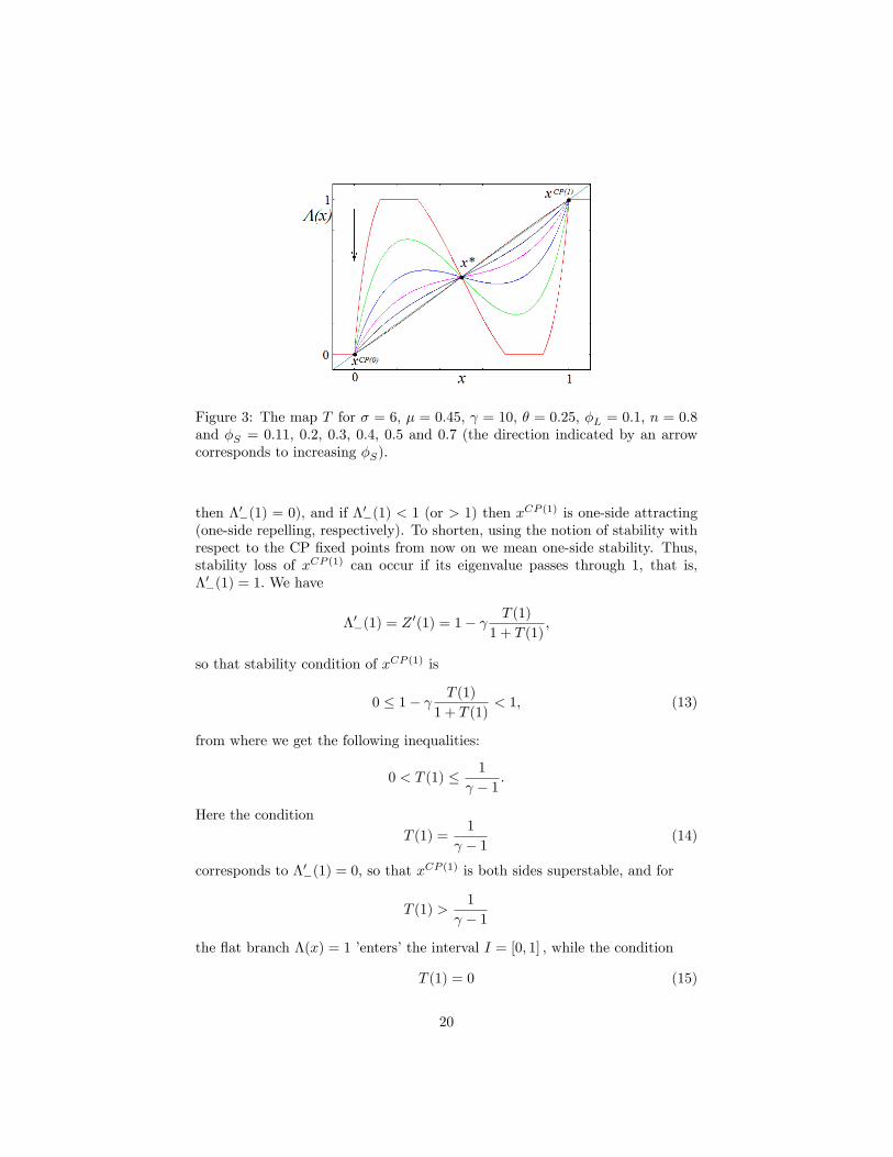
Figure 3: The map T for � = 6; � = 0:45; = 10; � = 0:25; �L = 0:1; n = 0:8and �S = 0:11; 0:2; 0:3; 0:4; 0:5 and 0:7 (the direction indicated by an arrowcorresponds to increasing �S).

then �0�(1) = 0), and if �0�(1) < 1 (or > 1) then x

CP (1) is one-side attracting(one-side repelling, respectively). To shorten, using the notion of stability withrespect to the CP �xed points from now on we mean one-side stability. Thus,stability loss of xCP (1) can occur if its eigenvalue passes through 1, that is,�0�(1) = 1: We have

�0�(1) = Z0(1) = 1� T (1)

1 + T (1);

so that stability condition of xCP (1) is

0 � 1� T (1)

1 + T (1)< 1; (13)

from where we get the following inequalities:

0 < T (1) � 1

� 1 :

Here the conditionT (1) =

1

� 1 (14)

corresponds to �0�(1) = 0; so that xCP (1) is both sides superstable, and for

T (1) >1

� 1

the �at branch �(x) = 1 �enters�the interval I = [0; 1] ; while the condition

T (1) = 0 (15)

20

is related to �0�(1) = 1; that is, to the stability loss of xCP (1): Given that this

�xed point always exists, this bifurcation cannot be related to a (one-side) foldbifurcation. As we shall see the �xed point xCP (1) losses stability due to a�one-side�transcritical bifurcation which we call border-transcritical bifurcation(see, for example, Fig.4 where the border-transcritical bifurcation is indicatedby green circles). It is associated with an asymmetric �xed point with whichxCP (1) merges at the bifurcation value and changes stability. The asymmetric�xed point can be born either due to a fold bifurcation, in which case it appearsin a couple with one more asymmetric �xed point (as, for example, in Fig.4cwhere the fold bifurcation is indicated by black circles), or due to pitchforkbifurcation of the symmetric �xed point x� (indicated in Fig.4 by red circles).In fact, the stability condition of x� de�ned by �1 < �0

�12

�< 1 is satis�ed for

�1 < 1 + 4T 0�1

2

�< 1 (16)

(to get this condition we�ve used the equality T�12

�= 0 which is easy to check),

or

� 8 < T 0

�1

2

�< 0: (17)

If

T 0�1

2

�= � 8

(18)

then �0�12

�= �1; so that x� undergoes a �ip bifurcation, while the equality

T 0�1

2

�= 0 (19)

is related to �0�12

�= 1; so that x� undergoes a pitchfork bifurcation (due to the

symmetry of the map fold or transcritical bifurcations cannot occur). In case ofsupercritical pitchfork bifurcation of x� the asymmetric �xed points x = xa andx = 1 � xa � x0a born due to this bifurcation are attracting (see, e.g., Fig.4a).Then the attracting �xed point x0a collides with repelling �xed point x

CP (1)

due to the border-transcritical bifurcation. In contrast, in the subcritical casetwo repelling �xed points x = xb and x = 1 � xb � x0b are born, and then therepelling �xed point x0b collides with the attracting �xed point x

CP (1) due tothe border-transcritical bifurcation (see, e.g., Fig.4b).In Sec.5.3 we present numerical results related to the mentioned above local

bifurcations, as well as results on global dynamics of the map � for the generalcase 0 < en � 1, while in the next subsection we assume en = 1 in which case it ispossible to get more analytical results on local stability of the �xed points (seealso Commendatore et al. [2012]).

21

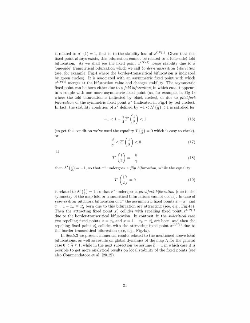
Figure 4: 1D bifurcation diagrams for �L = 0:1; n = 0:8; � = 6; � = 0:45; =10 and � = 0:05; �S 2 [0:3; 0:38] in a), � = 0:35; �S 2 [0:68; 0:7] in b), � = 0:18;�S 2 [0:6074; 0:6078] in c).

5.2 Stability of the �xed points: the case en = 1For en = 1 the condition (13) related to the stability of the CP �xed point xCP (1)can be written as

� 1

' < � < ' (20)

where

' =�

(� � �)[� + �S(1� 2�)] + [�(1� �) + ��]�2Sand � = �

���+1��1

S

For 1 < � < 1 + � and 0 � �S < 1, the right hand side inequality in (20)is always satis�ed; for � > 1 + � it can be shown that the right hand sideinequality in (20) is satis�ed for su¢ ciently high values of �S and violated forlow values (hint: we are dealing with two monotonically decreasing function of�S , the �rst, �(�S), tends to in�nity for �S ! 0 and it is equal to 1 at �S = 1;the second, '(�S), is positive (and larger than 1) but �nite at �S = 0 and it isequal to 1 at �S = 1. Since at �S = 1 the �rst derivative of the �rst functionis smaller in absolute value than the derivative of the second function, the twonecessarily cross at some �S = �trS , where 0 < �trS < 1). It is not possibleto specify the corresponding bifurcation value for the (internal) trade freeness

22

parameter �S explicitly, however, it is possible to �nd an explicit expression for�, see (28).For � > 1 + �, as �S crosses �

trS from left to right, the map � undergoes

a border-transcritical bifurcation: the CP �xed point xCP (1) merges with theasymmetric �xed point gaining stability. Symmetrically, xCP (0) meets the otherasymmetric �xed point gaining stability. From this we infer that the asymmetric�xed points must have always the same local stability properties in the neigh-borhood of the CP �xed points (as can be seen, for example, in Fig.7).The left hand side inequality in (20) holds for a su¢ ciently small value of :

<1

1� �'�1 :

When this latter condition does not hold, xCP (1) becomes both-side superstable.Moving on to the symmetric �xed point x�, recall that its local stability

requires that the condition (17) holds. Concerning the inequality on the righthand side of (17), we denote by �pfS that value of �S for which the conditionT 0�12

�= 0 is satis�ed. Moreover, �S < �

pfS implies T 0

�12

�< 0. For 0 < en < 1,

�pfS corresponds to the positive root of a quadratic equation whose expressionis quite complicated. From simulations we �nd that for some meaningful para-meter combinations, but not for all, 0 < �pfS < 1. For en = 1, we are able toobtain the following, relatively simple, expression:

�pfS =(� � �)[2�(� � 1)� �]

2�(� � �)(� � 1) + �(3� � 2 + �) < 1:

(In (27) we give the same condition solved with respect to the parameter �).One can show that- if 1 < � < 1+ �

2� , it follows that �pfS < 0. Therefore this inequality is never

satis�ed;- if � > 1 + �

2� , as �S crosses �pfS from left to right, the map � undergoes a

pitchfork bifurcation.A �rst interesting result is that, when en = 1, the local stability of the

symmetric �xed point does not depend on the trade distance with respect tothe outside region, as measured by the parameter �L. This result is a directconsequence of Proposition 1. The size of local demand (outside demand) inde-pendent of entrepreneurial migration (i.e. originating from immobile unskilledworkers), instead plays a relevant role, a¤ecting positively �pfS :

@�pfS@�

=4�(� � �)(2� � 1)(� � 1)

[2�(� � �)(� � 1) + �(3� � 2 + �)]2> 0:

This implies that increasing the size of local demand vis-à-vis that of outsidedemand has a stabilizing e¤ect on the symmetric �xed point and tends to favourdispersion (the opposite holds true by increasing outside demand with respectto local demand which has a destabilizing e¤ect on x� and tends to favouragglomeration).

23

The local stability properties of the symmetric equilibrium and, therefore,the characteristics of the bifurcation value determine the speci�c location pat-tern (see P�üger and Südekum [2008]) as trade integration between region 1 and2 intensi�es. The typical bifurcation scenario of a standard 2-region FE modelis catastrophic agglomeration, with an immediate jump to a Core-Peripheryequilibrium, corresponding to a subcritical pitchfork bifurcation. However, inour framework, a smoother agglomeration process can also emerge in correspon-dence of a supercritical pitchfork bifurcation with the emergence of two (locally)stable interior asymmetric equilibria.

In order to study in detail the properties of the pitchfork bifurcation, eventhough only for the case en = 1, we �rst rede�ne our central map to highlightthe control parameter we are interested in, the trade freeness parameter �S ,and we verify how these may change when another crucial parameter, the sizeof local demand (at least, that part that it is not a¤ected by entrepreneurialmovements and that originates from immobile unskilledworkers) �, varies. Therede�ned map is:

Z(�S ; x) =

�1 + (1� x) T (�S ; x)

1 + xT (�S ; x)

�From the theory of dynamical systems (see e.g., Wiggins [2013]), in corre-

spondence of a pitchfork bifurcation, that is, when �S = �pfS and x = 12 , the

following conditions must hold:

1. @Z@�S

��pfS ;

12

�= 0 , @T

@�S

��pfS ;

12

�= 0;

2. @2Z@x2

��pfS ;

12

�= 0 , @2T

@x2

��pfS ;

12

�= 0;

3. @2Z@x@�S

��pfS ;

12

�6= 0 , @2T

@x@�S

��pfS ;

12

�6= 0;

4. @3Z@x3

��pfS ;

12

�6= 0 , @3T

@x3

��pfS ;

12

�6= 0:

Moreover, the sign of the following expression can be used to determine onwhich side of �pfS the asymmetric �xed points, at least initially, lie:

5. �@3Z@x3(�pfS ; 12 )

@2Z@x@�S

(�pfS ; 12 )> (<)0, �

@3T@x3(�pfS ; 12 )

@2T@x@�S

(�pfS ; 12 )> (<)0:

When this expression is larger (less) than zero, the pitchfork bifurcation issupercritical (subcritical); for the particular case

@3Z

@x3

��pfS ;

1

2

�= 0 (21)

24

the pitchfork bifurcation is critical7 (for example, in Fig.6 the intersection pointof the pitchfork and fold bifurcation curves � = �pf and � = �f is a codimention-2 bifurcation point at which the pitchfork bifurcation is critical: it occurs si-multaneously with two fold bifurcations). We have that:- Condition 1 is veri�ed due to the fact that at the symmetric equilibrium

V1 = V2 and @V1@�S

= @V2@�S

for any �S ;

- Condition 2 is veri�ed due to the symmetric properties of the map Z(x).Indeed, at the bifurcation point, this condition can be reduced to:

@2V1@x2 �

@2V2@x2 =

@2�

�1P�1

�@x2 �

@2�

�2P�2

�@x2 = �(1 + �)

�( @�1@x )

2

P�+21

�1 �( @�2@x )

2

P�+22

�2

��

2�

�@�1@x

@P1@x

P�+11

�@�2@x

@P2@x

P�+12

�+

�@2�1@x2

P�1�

@2�2@x2

P�2

�� �

�@2P1@x2

P�+11

�1 �@2P2@x2

P�+12

�2

�= 0;

which holds, given that at x = 12 :

�1 = �2, P1 = P2, @�1@x = �@�2@x ,

@P1@x = �@P2

@x ,@2�1@x2 =

@2�2@x2 and

@2P1@x2 =

@2P2@x2 .

Note that both conditions 1 and 2 hold also for the case 0 < en < 1;- Concerning condition 3 we obtain the following result:

@2T

@x@�S

��pfS ;

1

2

�=

=2�(2� � 1)[(� � 1)(� � �)2� + �(�+ 3� � 2)]2

(� � �)(� � 1)2(�+ 2��)[(� � 1)(� � �)2� + �(� � 1 + �)] > 0

which is always satis�ed;

- Concerning condition 4 we obtain the following result:@3T@x3

��pfS ;

12

�=

=32�4(2��1)3f12(��1)2(���)�2+[2(2��3)�2+4(3���)(��1)2]���(��1+�)[2(��1)+�]g

(��1)3(�+2��)[(��1)(���)2�+�(��1+�)]3According to this expression condition 4 may or may not hold depending onparameter combinations;

- Finally, considering condition 5, the sign of @3T@x3

��pfS ;

12

�coincides with

that of the following expression:

K = 12(� � 1)2(� � �)�2 + [2(2� � 3)�2++4(3�� �)(� � 1)2]� � �(� � 1 + �)[2(� � 1) + �]: (22)

This allows us to state the following

Proposition 2 Let�s assume that � > 1 + �. Then there exists a value of theparameter � = � with 0 < � < 1

2 such that K < 0 for � < �, K > 0 for � > �,and K = 0 for � = �, where K is given in (22).

7 If the condition (21) holds not only for x = 12; but for also in some neighborhood of

x = 12, this means so-called degenerate pitchfork bifurcation (see Sushko and Gardini [2010])

as sketched, for example, in Fig.7, that cannot occur in the considered map.

25

Proof. First we consider the following second degree equation based on (22):

a�2 + b� + c = 0; (23)

where

a = 12(� � 1)2(� � �) > 0;b = 2(2� � 3)�2 + 4(3�� �)(� � 1)2 � (<)0;c = ��(� � 1 + �)[2(� � 1) + �] < 0:

Therefore (23) admits one positive and one negative solution. In order to havereal roots, it must be:

� = b2�4ac = (12��8�2�3)�4+4(10�2�12�+3)(��1)2�2+4�2(��1)4 > 0:

� = 0 is a quartic equation that admits four solutions of which only two atmost are real (or none). De�ne y = �2. Then we can write:

� = b2�4ac = (12��8�2�3)y2+4(10�2�12�+3)(��1)2y+4�2(��1)4 = 0:(24)

This is now a second degree equation whose solutions, y1 and y2, are real sincee� = 144(3� � 1)(2� � 1)2(2� � 1)5 > 0:Moreover, these solutions are both negative for 1 < � < 3+

p3

4 and one positive

and one negative for � > 3+p3

4 , i.e. y2 < 0 < y1: Therefore, for 1 < � < 3+p3

4 ,

� > 0 always; and for � > 3+p3

4 , � > 0 as long as 0 < x < 1 < x1. Thereforealso in this case � > 0 for all relevant values of �.8

Therefore, (23) admits two real solutions, one positive and one negative.Let�s call the positive solution �, where � = � b�

p�

2a . Given that a > 0, we haveK < 0 for 0 < � < � and K > 0 for � > �; and K = 0 when � = �, where K isgiven in (22).Finally, notice that the condition � < 1

2 corresponds to

4(� + �)(�+ � � 1)[� � (1 + �)] > 0:

That can be further reduced to � � (1 + �) > 0.

Q.E.D.

In summary, the size of local (immobile) demand matters with respect tooutside (immobile) demand determining the location pattern at the bifurcation

8Note that x2 > 1 as long as the sum of the coe¢ cients in the equation (24) is positive,that is,

4�6 � 16�5 + 64�4 � 144�3 + 144�2 � 60� + 9 > 0Looking at the solutions of the six degrees equation, none of them is real. It follows that thisinequality is always satis�ed or never satis�ed. It is immediate to check, by substituting anynumber for �, that the condition holds.

26

point, which is catastrophic when the size of local demand is su¢ ciently largein relative terms and it is smooth when it is the size of outside demand thatbecomes su¢ ciently large in relative terms (see Fig.7c and b, where we assume� = 0:4 and � = 0:32, respectively). We envisage that, by continuity, a similarresult must hold also when we allow for a local manufacturing sector in region3. Indeed Fig. 4 con�rms for the case 0 < en < 1 the possible occurrence ofthese bifurcation scenarios.

Finally, concerning the inequality on the left hand side of (17), it holds fora su¢ ciently small value of or for a su¢ ciently high value of �. When thiscondition does not hold, a �ip bifurcation scenario emerges, with the possibleoccurrence of complex behavior, involving the global properties of dynamics.We turn now to such type of analysis.

5.3 Numerical results

In this section we study local and global dynamics of the map � in generic case.Recall that � depends on 7 parameters satisfying the following conditions:

� > 1; > 0; 0 < �; �S ; �L; en < 1; 0 < � < 1=2; �L � �S :Our main interest is related to the in�uence on dynamics of the parameters �S ,�L, n and �, so, we can �x the other parameters as follows:

� = 6; � = 0:45; = 10; (25)

and investigate bifurcation structure of the remaining parameter space by meansof 1D and 2D bifurcation diagrams. This analysis extends the results of the caseen = 1 to that of en < 1, when the manufacturing sector is also located in theoutside region.First, in Fig.5 we show a 2D bifurcation diagram in the (�S ; �)-parameter

plane for �L = 0:1 and en = 0:8: Here di¤erent colors are related to di¤erentattracting cycles, namely, the red region S to the symmetric �xed point x�;the pink region AS to coexisting asymmetric �xed points xa and x0a; the blueregion CP1 to the Core-Periphery �xed points xCP (0) and xCP (1); the blueregion CP2 to the �xed points xCP (0) and xCP (1) which are locally repellingbut represent attractors in Milnor sense; the green region to 2-cycles; the othercolors correspond to cycles of periods k � 30 and white region is related eitherto higher periodicity or to chaotic attractors. Clearly, the upper boundary of theregion S in Fig.5 is related to the �ip bifurcation of x�; while its lower boundaryis the pitchfork bifurcation curve. In the following subsections we discuss bothscenarios in detail.Before doing so, let us brie�y summarize the economic interpretations that

can be drawn from Fig. 5: for high free tradess inside the Union (i.e. for ahigh value of �S) agglomeration of economic activities in one of the two regionsof the Union is a likely outcome; lowering this parameter leads to an equaldistribution of economic activities (if �S enters in the red area S) or to an

27

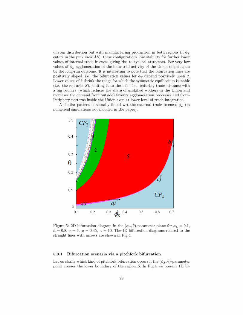
uneven distribution but with manufacturing production in both regions (if �Senters in the pink area AS); these con�gurations lose stability for further lowervalues of internal trade freeness giving rise to cyclical attractors. For very lowvalues of �S agglomeration of the industrial activity of the Union might againbe the long-run outcome. It is interesting to note that the bifurcation lines arepositively sloped, i.e. the bifurcation values for �S depend positively upon �.Lower values of � shrink the range for which the symmetric equilibrium is stable(i.e. the red area S), shifting it to the left ; i.e. reducing trade distance witha big country (which reduces the share of unskilled workers in the Union andincreases the demand from outside) favours agglomeration processes and Core-Periphery patterns inside the Union even at lower level of trade integration.A similar pattern is actually found wrt the external trade freeness �L (in

numerical simulations not incuded in the paper).

Figure 5: 2D bifurcation diagram in the (�S ; �)-parameter plane for �L = 0:1;en = 0:8; � = 6; � = 0:45; = 10: The 1D bifurcation diagrams related to thestraight lines with arrows are shown in Fig.4.

5.3.1 Bifurcation scenario via a pitchfork bifurcation

Let us clarify which kind of pitchfork bifurcation occurs if the (�S ; �)-parameterpoint crosses the lower boundary of the region S: In Fig.4 we present 1D bi-

28

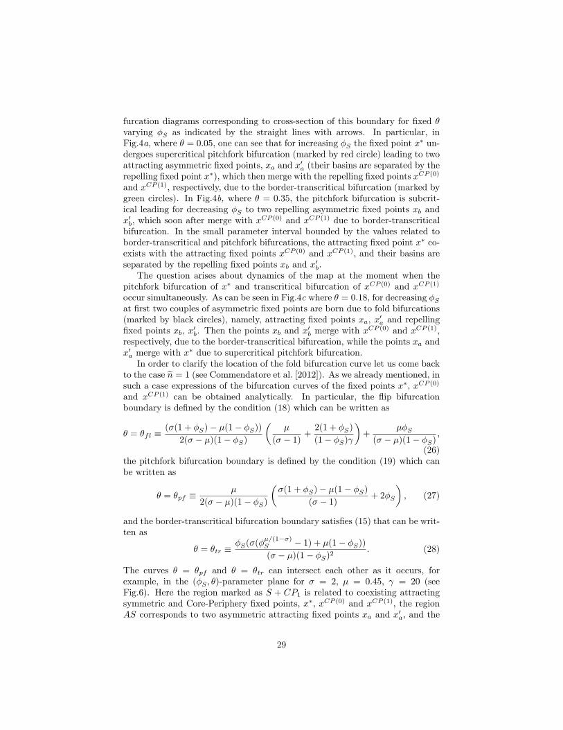
furcation diagrams corresponding to cross-section of this boundary for �xed �varying �S as indicated by the straight lines with arrows. In particular, inFig.4a, where � = 0:05, one can see that for increasing �S the �xed point x

� un-dergoes supercritical pitchfork bifurcation (marked by red circle) leading to twoattracting asymmetric �xed points, xa and x0a (their basins are separated by therepelling �xed point x�), which then merge with the repelling �xed points xCP (0)

and xCP (1); respectively, due to the border-transcritical bifurcation (marked bygreen circles). In Fig.4b, where � = 0:35; the pitchfork bifurcation is subcrit-ical leading for decreasing �S to two repelling asymmetric �xed points xb andx0b, which soon after merge with x

CP (0) and xCP (1) due to border-transcriticalbifurcation. In the small parameter interval bounded by the values related toborder-transcritical and pitchfork bifurcations, the attracting �xed point x� co-exists with the attracting �xed points xCP (0) and xCP (1); and their basins areseparated by the repelling �xed points xb and x0b:The question arises about dynamics of the map at the moment when the

pitchfork bifurcation of x� and transcritical bifurcation of xCP (0) and xCP (1)

occur simultaneously. As can be seen in Fig.4c where � = 0:18, for decreasing �Sat �rst two couples of asymmetric �xed points are born due to fold bifurcations(marked by black circles), namely, attracting �xed points xa, x0a and repelling�xed points xb, x0b. Then the points xb and x

0b merge with x

CP (0) and xCP (1);respectively, due to the border-transcritical bifurcation, while the points xa andx0a merge with x

� due to supercritical pitchfork bifurcation.In order to clarify the location of the fold bifurcation curve let us come back

to the case en = 1 (see Commendatore et al. [2012]). As we already mentioned, insuch a case expressions of the bifurcation curves of the �xed points x�; xCP (0)

and xCP (1) can be obtained analytically. In particular, the �ip bifurcationboundary is de�ned by the condition (18) which can be written as

� = �fl �(�(1 + �S)� �(1� �S))

2(� � �)(1� �S)

��

(� � 1) +2(1 + �S)

(1� �S)

�+

��S(� � �)(1� �S)

;

(26)the pitchfork bifurcation boundary is de�ned by the condition (19) which canbe written as

� = �pf ��

2(� � �)(1� �S)

��(1 + �S)� �(1� �S)

(� � 1) + 2�S

�; (27)

and the border-transcritical bifurcation boundary satis�es (15) that can be writ-ten as

� = �tr ��S(�(�

�=(1��)S � 1) + �(1� �S))(� � �)(1� �S)2

: (28)

The curves � = �pf and � = �tr can intersect each other as it occurs, forexample, in the (�S ; �)-parameter plane for � = 2; � = 0:45; = 20 (seeFig.6). Here the region marked as S + CP1 is related to coexisting attractingsymmetric and Core-Periphery �xed points, x�; xCP (0) and xCP (1); the regionAS corresponds to two asymmetric attracting �xed points xa and x0a; and the

29

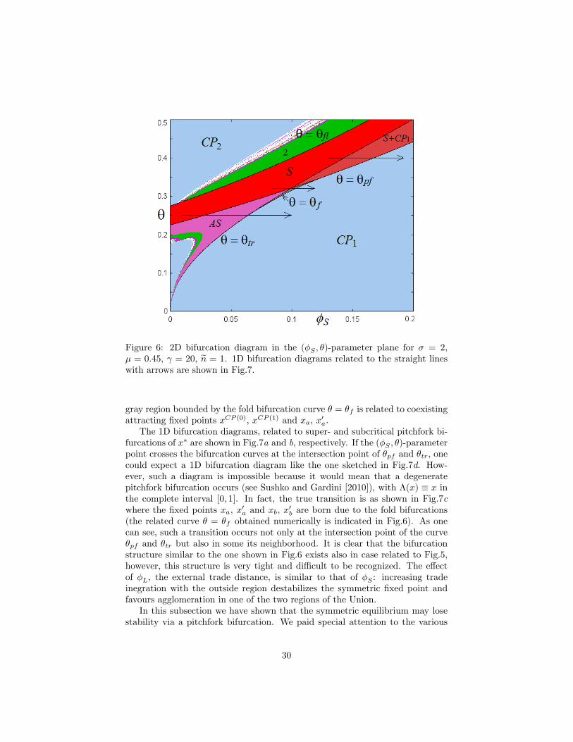
Figure 6: 2D bifurcation diagram in the (�S ; �)-parameter plane for � = 2;� = 0:45; = 20; en = 1. 1D bifurcation diagrams related to the straight lineswith arrows are shown in Fig.7.

gray region bounded by the fold bifurcation curve � = �f is related to coexistingattracting �xed points xCP (0); xCP (1) and xa; x0a.The 1D bifurcation diagrams, related to super- and subcritical pitchfork bi-

furcations of x� are shown in Fig.7a and b, respectively. If the (�S ; �)-parameterpoint crosses the bifurcation curves at the intersection point of �pf and �tr; onecould expect a 1D bifurcation diagram like the one sketched in Fig.7d. How-ever, such a diagram is impossible because it would mean that a degeneratepitchfork bifurcation occurs (see Sushko and Gardini [2010]), with �(x) � x inthe complete interval [0; 1]. In fact, the true transition is as shown in Fig.7cwhere the �xed points xa; x0a and xb, x

0b are born due to the fold bifurcations

(the related curve � = �f obtained numerically is indicated in Fig.6). As onecan see, such a transition occurs not only at the intersection point of the curve�pf and �tr but also in some its neighborhood. It is clear that the bifurcationstructure similar to the one shown in Fig.6 exists also in case related to Fig.5,however, this structure is very tight and di¢ cult to be recognized. The e¤ectof �L, the external trade distance, is similar to that of �S : increasing tradeinegration with the outside region destabilizes the symmetric �xed point andfavours agglomeration in one of the two regions of the Union.In this subsection we have shown that the symmetric equilibrium may lose

stability via a pitchfork bifurcation. We paid special attention to the various

30

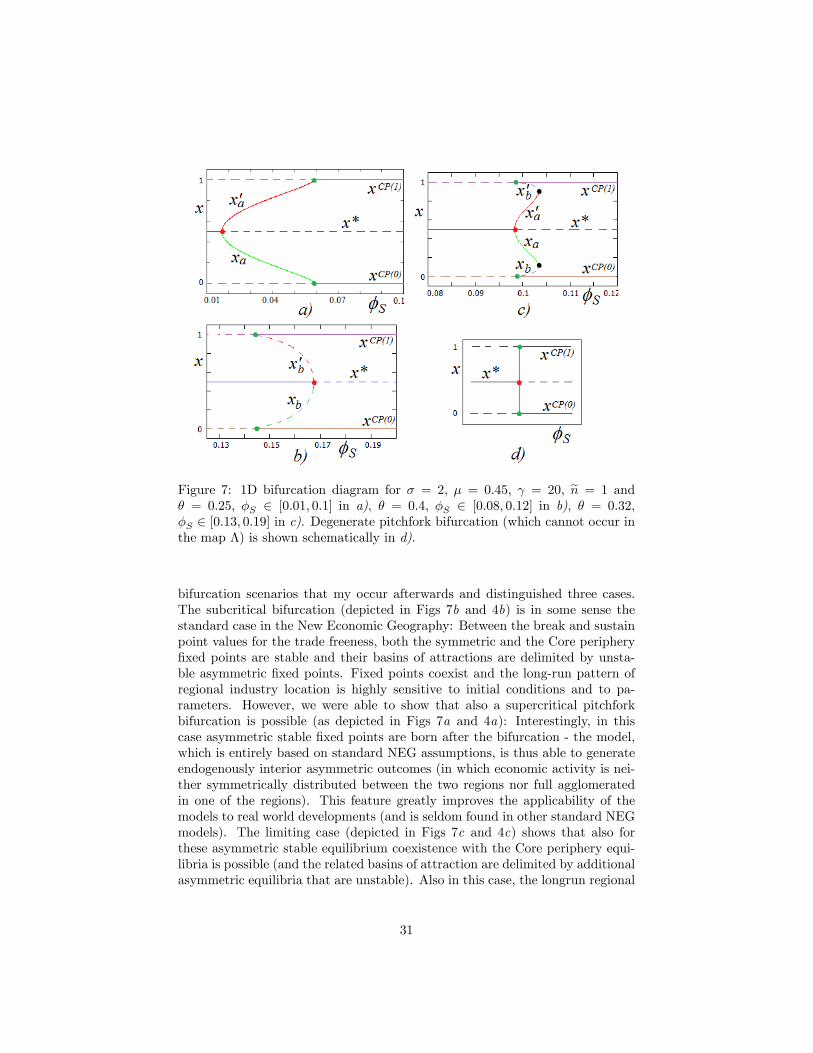
Figure 7: 1D bifurcation diagram for � = 2; � = 0:45; = 20; en = 1 and� = 0:25; �S 2 [0:01; 0:1] in a), � = 0:4; �S 2 [0:08; 0:12] in b), � = 0:32;�S 2 [0:13; 0:19] in c). Degenerate pitchfork bifurcation (which cannot occur inthe map �) is shown schematically in d).

bifurcation scenarios that my occur afterwards and distinguished three cases.The subcritical bifurcation (depicted in Figs 7b and 4b) is in some sense thestandard case in the New Economic Geography: Between the break and sustainpoint values for the trade freeness, both the symmetric and the Core periphery�xed points are stable and their basins of attractions are delimited by unsta-ble asymmetric �xed points. Fixed points coexist and the long-run pattern ofregional industry location is highly sensitive to initial conditions and to pa-rameters. However, we were able to show that also a supercritical pitchforkbifurcation is possible (as depicted in Figs 7a and 4a): Interestingly, in thiscase asymmetric stable �xed points are born after the bifurcation - the model,which is entirely based on standard NEG assumptions, is thus able to generateendogenously interior asymmetric outcomes (in which economic activity is nei-ther symmetrically distributed between the two regions nor full agglomeratedin one of the regions). This feature greatly improves the applicability of themodels to real world developments (and is seldom found in other standard NEGmodels). The limiting case (depicted in Figs 7c and 4c) shows that also forthese asymmetric stable equilibrium coexistence with the Core periphery equi-libria is possible (and the related basins of attraction are delimited by additionalasymmetric equilibria that are unstable). Also in this case, the longrun regional

31

distribution of industrial activity is highly sensitive upon initial conditions andon parameters.Note that we discussed these phenomena wrt a change in the interior trade

freeness (between the two regions of our integration area). However, qualita-tively similar results can be obtain for a variation of the exterior trade freenessand for the (mobile) share of entrepreneurs and of unquali�ed workers. Chang-ing any of these parameters may lead to asymmetric stable equilibria that maycoexist with stable CP equilibria.

5.3.2 Bifurcation scenario related to a �ip bifurcation

In this section we discuss the second type of bifurcation that may lead to astability loss of the symetric �xed point - the �ip bifrucation. We show that themap can have attracting cycles and chaotic attractors, and that coexistence ofattractors may actually involve either cycles or chaotic attractors with complexbasins of attractions.In order to comment bifurcation scenario which is observed in the map �

if the parameter point crosses the �ip bifurcation boundary of the parameterregion S; that is, when the symmetric �xed point x� undergoes the �ip bifur-cation, we show in Fig.8 the bifurcation structure for �xed �; �; (see (25)) inthe (�S ; en)-parameter plane for � = 0:25; �L = 0:01 in a), and in the (�L; en)-parameter plane for � = 0:25, �S = 0:15 in b). Note from these Figures a similare¤ect of varying the internal and external trade freeness as in Figure 5 thus cor-roborating the conclusions drawn above: For high trade freeness (in particularinside the Union) agglomeration is the most likely outcome for industrial loca-tion; reducing trade freeness leads �rst to a stable symmetric equilibrium; thenit gives rise to cyclical solutions; and �nally to a full agglomeration outcome. Itis interesting to see that the e¤ect of increasing en (i.e. the relative size of theindustrial sector inside the Union) has a non-monotonic e¤ect: starting from alow (high) value, increasing en shifts the stable range for the symmetric equilib-rium towards higher (lower) values of trade freeness. For a highly industrializedUnion (en close to 1) the bifurcation curves are negatively sloped, implying thatthe bifurcation values for both dimensions of trade freeness (internal and exter-nal) depend negatively upon its industrial share in the overall economy. Thus,if there is a shift in the Union�s trading partners towards lower industrializedregions (en getting even closer to 1), a Core-Periphery long-run position becomesless likely.Let us consider the 1D bifurcation diagram related to the cross-section indi-

cated in Fig.8 by the straight line with an arrow. It is shown in Fig.9 togheterwith an enlargement.One can see in Fig.9a that for decreasing �S the �xed point x

� undergoesa supercritical �ip bifurcation (at the point marked by black circle) leading toan attracting 2-cycle g2 = fx0; x1g; whose points are symmetric with respectto x�. Then g2 undergoes a supercritical pitchfork bifurcation (at the pointmarked by red circle), due to which two new attracting 2-cycles q2 and q02 areborn, points of which are symmetric to each other with respect to x�: If we

32

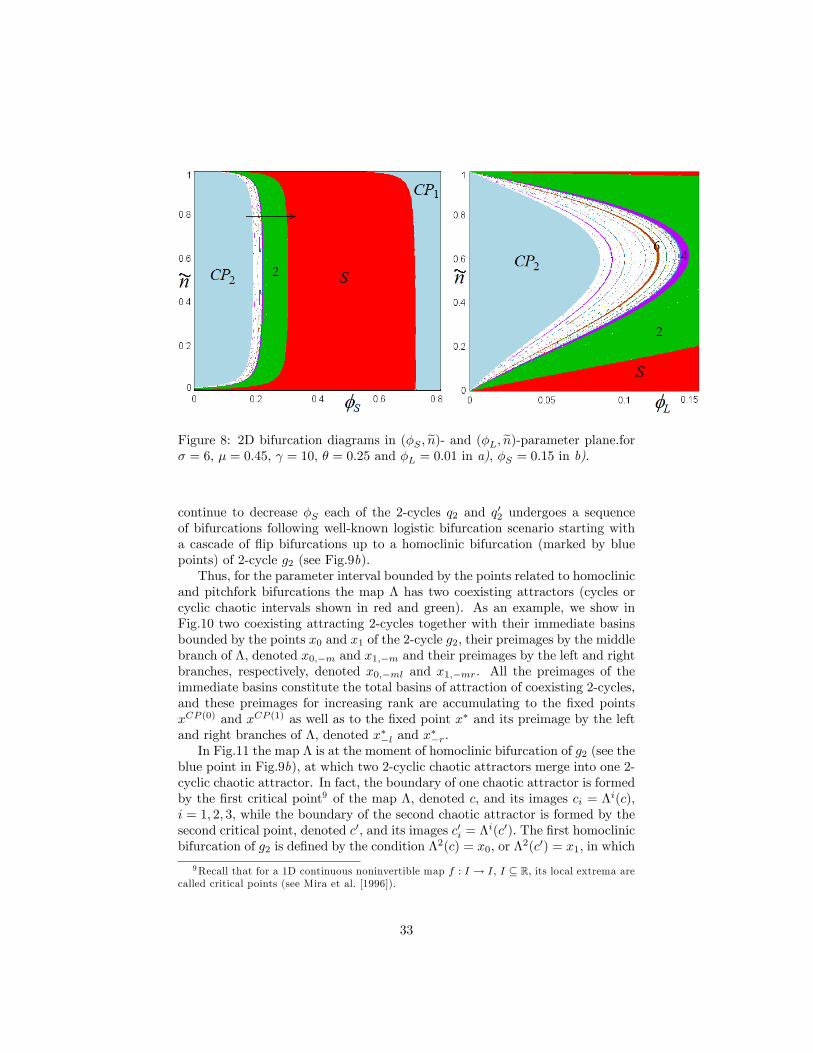
Figure 8: 2D bifurcation diagrams in (�S ; en)- and (�L; en)-parameter plane.for� = 6; � = 0:45; = 10; � = 0:25 and �L = 0:01 in a), �S = 0:15 in b).

continue to decrease �S each of the 2-cycles q2 and q02 undergoes a sequence

of bifurcations following well-known logistic bifurcation scenario starting witha cascade of �ip bifurcations up to a homoclinic bifurcation (marked by bluepoints) of 2-cycle g2 (see Fig.9b).Thus, for the parameter interval bounded by the points related to homoclinic

and pitchfork bifurcations the map � has two coexisting attractors (cycles orcyclic chaotic intervals shown in red and green). As an example, we show inFig.10 two coexisting attracting 2-cycles together with their immediate basinsbounded by the points x0 and x1 of the 2-cycle g2; their preimages by the middlebranch of �; denoted x0;�m and x1;�m and their preimages by the left and rightbranches, respectively, denoted x0;�ml and x1;�mr. All the preimages of theimmediate basins constitute the total basins of attraction of coexisting 2-cycles,and these preimages for increasing rank are accumulating to the �xed pointsxCP (0) and xCP (1) as well as to the �xed point x� and its preimage by the leftand right branches of �, denoted x��l and x

��r.

In Fig.11 the map � is at the moment of homoclinic bifurcation of g2 (see theblue point in Fig.9b), at which two 2-cyclic chaotic attractors merge into one 2-cyclic chaotic attractor. In fact, the boundary of one chaotic attractor is formedby the �rst critical point9 of the map �; denoted c; and its images ci = �i(c);i = 1; 2; 3; while the boundary of the second chaotic attractor is formed by thesecond critical point, denoted c0; and its images c0i = �

i(c0): The �rst homoclinicbifurcation of g2 is de�ned by the condition �2(c) = x0, or �2(c0) = x1; in which

9Recall that for a 1D continuous noninvertible map f : I ! I; I � R; its local extrema arecalled critical points (see Mira et al. [1996]).

33

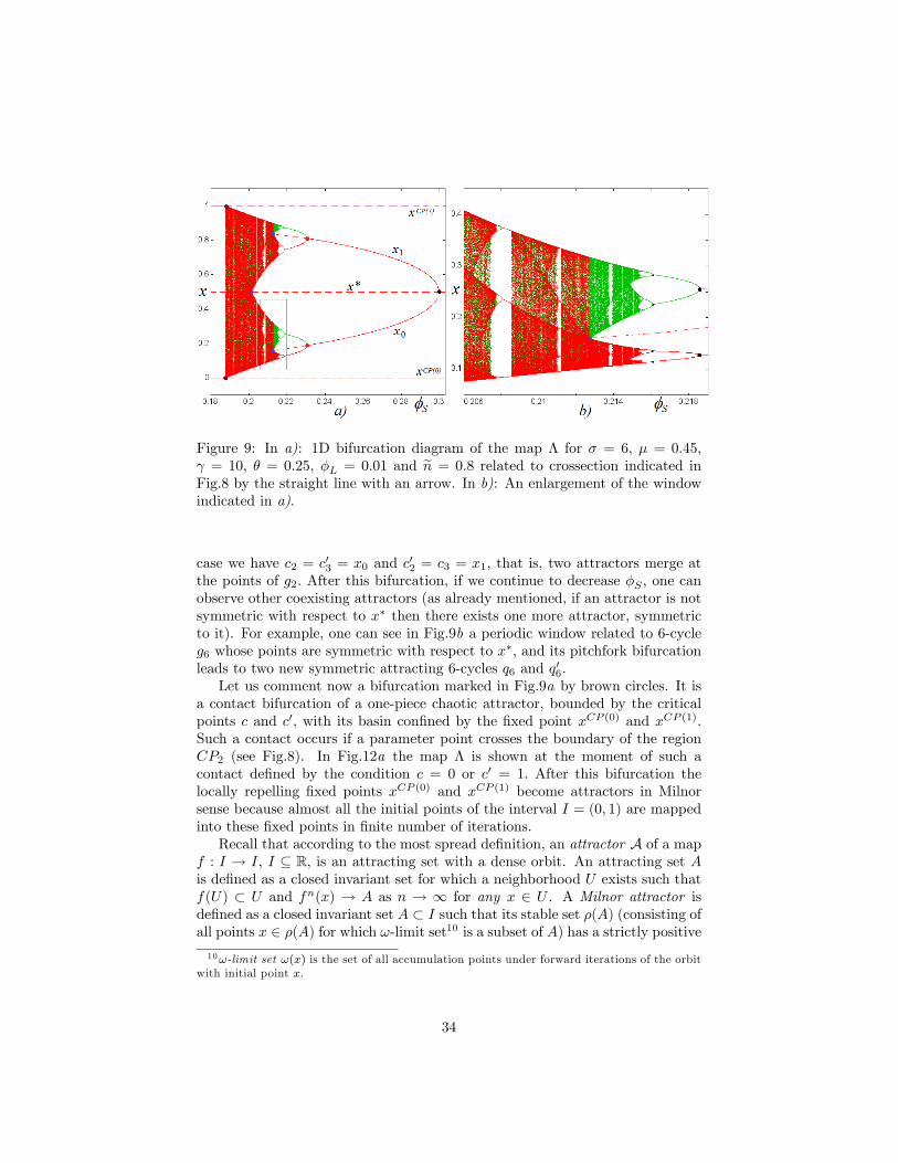
Figure 9: In a): 1D bifurcation diagram of the map � for � = 6; � = 0:45; = 10; � = 0:25, �L = 0:01 and en = 0:8 related to crossection indicated inFig.8 by the straight line with an arrow. In b): An enlargement of the windowindicated in a).

case we have c2 = c03 = x0 and c02 = c3 = x1; that is, two attractors merge atthe points of g2: After this bifurcation, if we continue to decrease �S ; one canobserve other coexisting attractors (as already mentioned, if an attractor is notsymmetric with respect to x� then there exists one more attractor, symmetricto it). For example, one can see in Fig.9b a periodic window related to 6-cycleg6 whose points are symmetric with respect to x�; and its pitchfork bifurcationleads to two new symmetric attracting 6-cycles q6 and q06.Let us comment now a bifurcation marked in Fig.9a by brown circles. It is

a contact bifurcation of a one-piece chaotic attractor, bounded by the criticalpoints c and c0; with its basin con�ned by the �xed point xCP (0) and xCP (1).Such a contact occurs if a parameter point crosses the boundary of the regionCP2 (see Fig.8). In Fig.12a the map � is shown at the moment of such acontact de�ned by the condition c = 0 or c0 = 1: After this bifurcation thelocally repelling �xed points xCP (0) and xCP (1) become attractors in Milnorsense because almost all the initial points of the interval I = (0; 1) are mappedinto these �xed points in �nite number of iterations.Recall that according to the most spread de�nition, an attractor A of a map

f : I ! I; I � R; is an attracting set with a dense orbit. An attracting set Ais de�ned as a closed invariant set for which a neighborhood U exists such thatf(U) � U and fn(x) ! A as n ! 1 for any x 2 U . A Milnor attractor isde�ned as a closed invariant set A � I such that its stable set �(A) (consisting ofall points x 2 �(A) for which !-limit set10 is a subset of A) has a strictly positive10!-limit set !(x) is the set of all accumulation points under forward iterations of the orbit

with initial point x.

34

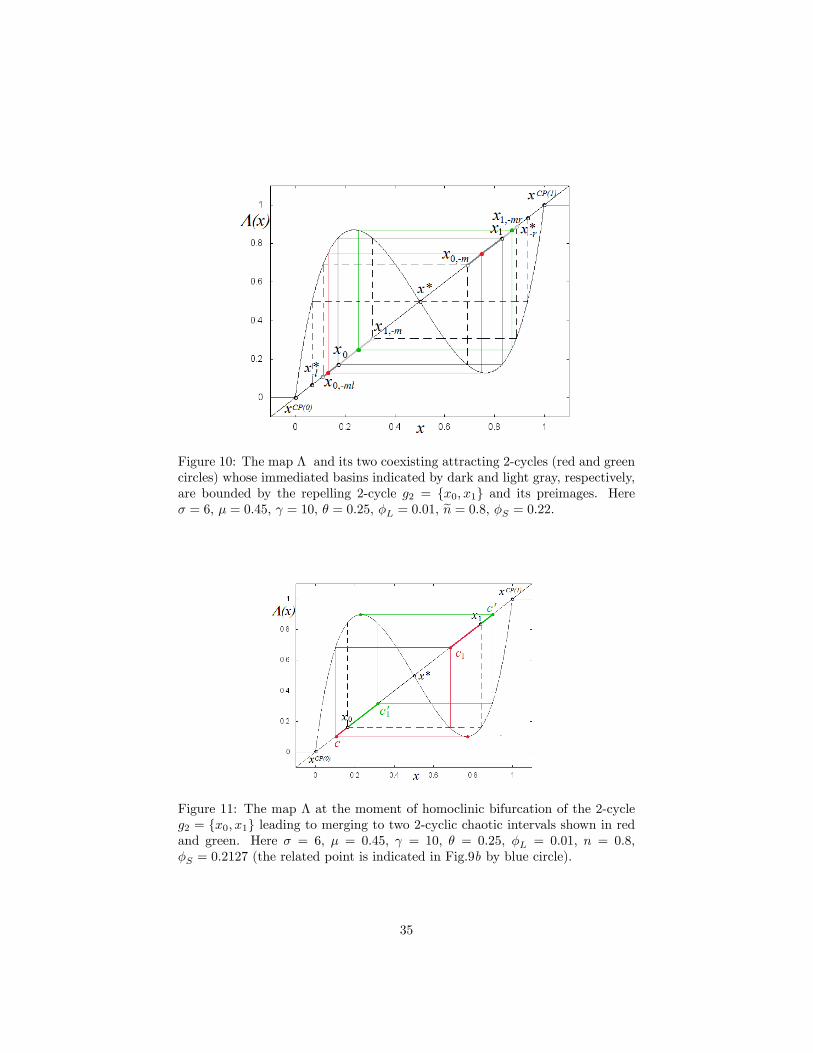
Figure 10: The map � and its two coexisting attracting 2-cycles (red and greencircles) whose immediated basins indicated by dark and light gray, respectively,are bounded by the repelling 2-cycle g2 = fx0; x1g and its preimages. Here� = 6; � = 0:45; = 10; � = 0:25, �L = 0:01; en = 0:8; �S = 0:22.

Figure 11: The map � at the moment of homoclinic bifurcation of the 2-cycleg2 = fx0; x1g leading to merging to two 2-cyclic chaotic intervals shown in redand green. Here � = 6; � = 0:45; = 10; � = 0:25, �L = 0:01; n = 0:8;�S = 0:2127 (the related point is indicated in Fig.9b by blue circle).

35

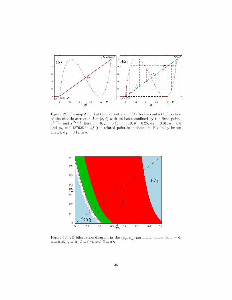
Figure 12: The map � in a) at the moment and in b) after the contact bifurcationof the chaotic attractor A = [c; c0] with its basin con�ned by the �xed pointsxCP (0) and xCP (1): Here � = 6; � = 0:45; = 10; � = 0:25, �L = 0:01; en = 0:8and �S = 0:187626 in a) (the related point is indicated in Fig.9a by browncircle), �S = 0:18 in b).

Figure 13: 2D bifurcation diagram in the (�S ; �L)-parameter plane for � = 6;� = 0:45; = 10; � = 0:25 and en = 0:8:

36

measure, and there is no strictly smaller closed subset A0 of A such that �(A0)coincides with �(A) up to a set of measure zero (see Milnor [1985]). As we see,the basic di¤erence of these two de�nitions of an attractor is related to the factthat in the �rst case any point from a neighborhood of A is attracted to A, whilein case of a Milnor attractor not necessarily all the points from a neighborhoodof A are attracted to it (in fact, the class of Milnor attractors is wider and itincludes the sets which are attractors according to the �rst de�nition).For example, one can see in Fig.12b that the points of the green intervals

are mapped into xCP (1) and the points of the red intervals are mapped intoxCP (0): In fact, the interval J1 related to the left �at branch of � and all itspreimages (a few of which are shown in Fig.12b) constitute the stable set ofthe �xed point xCP (1). There is a sequence of preimages of J1 accumulating toxCP (0), and there is also a sequence of preimages of J1 accumulating to xCP (1):The same can be said about sequences of preimages of J2 related to the second�at branch of �. Thus, in any (one-side) neighborhood of xCP (0) or xCP (1) thereis a set of positive measure of points which �rst escape from this neighborhoodand then eventually are mapped to xCP (0); as well a symmetric set of positivemeasure of points mapped to xCP (1): Clearly, not all the point of I are mappedto xCP (0) or xCP (1): a chaotic repellor, separating the basins of the CP �xedpoints, remains in I; which is a Cantor set formed by all the repelling cyclesand their preimages, as well as uncountably many aperiodic orbits.In Fig.13 we show bifurcation structure of the (�S ; �L)-parameter plane for

�xed �; �; (see (25)) and � = 0:25; en = 0:8. Recall that the inequality�S � �L has to be satis�ed, thus, the region above the straight line �S =�L is not valid. As one can see, qualitative structures of all the presented2D bifurcation diagrams are quite similar, so that we can suggest that thebifurcation scenario observed crossing the pitchfork bifurcation boundary ofthe region S is qualitatively similar to the one shown in Fig.4, while if the �ipbifurcation boundary of the region S is crossed then the scenario is qualitativelysimilar to the one illustrated in Fig.9a.This Figure allows us to comment on the interaction between the two di-

mensions of trade freeness (external and internal): the negative slope of thebifurcation curves implies that the bifurcation values for �S is decreasing in �Land the stable range of the symmetric equilibrium (the area S) shifts to theleft for higher values of �L. This gives a clear hint that agglomeration is themost likely outcome of a symultaneous process of regional integration withinthe Union and external trade liberalisation.

6 Conclusions

The EU has experienced a strong trend of deepening internal economic inte-gration, including trade and factor mobility. At the same time, the ongoingstrategy �Global Europe� aims at reducing trade barriers with respect to therest of the World. Furthermore, deeper EU integration into the world economyis currently characterised by the increasing importance of trade partners en-

37

dowed with relatively lower levels of technology and higher shares of unskilledworkers.Given these stylised facts, our research question was to analyse the e¤ects

of deeper regional integration and international liberalisation within the sametheoretical framework, especially shedding light on the importance of the en-dowments of the external trade partners.To this end, this paper has presented a 3-region FE-NEG model aiming to

study the interaction of commodity trade and factor mobility under the assump-tion �that is in line with stylized facts for EU �of mobile entrepreneurs/highquali�ed workers and immobile less quali�ed workers. The model has been setin discrete time and we studied the dynamic processes involved.In the model, the world economy includes an economically integrated area

composed of two regions �the Union �and an outside region. The two regions ofthe Union are closely integrated by means of lower mutual trade costs and mobileentrepreneurs. The outside region is separated from the Union due to high tradecosts and immobile entrepreneurs. We paid particular attention to regionalendowments of entrepreneurs and low quali�ed workers, considering the outsideregion not having a manufacturing sector as limiting case. Despite the analyticalcomplexity typical for NEG models, we derived some results analytically while,for other results, we had to use simulations as standard in the NEG literature.A �rst set of results is related to the existence and properties of the multiple

equilibria which are a typical outcome of NEG models:Most remarkably, our model � although being entirely based on standard

NEG assumption �is able to endogenously generate, for signi�cant parameterranges, asymmetric stable equilibria, i.e. long-term positions in which the eco-nomic activity is still present in both regions of the Union even though it is notdistributed symmetrically. This result is analytically derived for the special casein which the outside region is a pure rural economy without a manufacturingsector. Simulations show that it carries over to the general case.For the standard NEG long-run equilibria, i.e. for the symmetric and the core

periphery equilibria, we take a closer look at the employment structure: We canshow that they respond in a usual Heckscher-Ohlin way to changes in the relativeendowments: increasing the share of the mobile high quali�ed entrepreneurs ordecreasing the share of low quali�ed labor favors the employment share of themanufacturing sector in the resp region. This result holds although the model isspeci�ed in the NEG perspective. Also, it can be shown that trade costs matter �e.g. a reduction in internal trade costs fosters manufacturing in the two regions�Union (driving the economic activities away from the outside region).Another set of results pertains to the analysis of the local and global dy-

namics of the speci�ed factor mobility process within the Union.Surprisingly, we found that the basic bifurcation scenarios are qualitatively

similar in all the parameter planes which we considered. It is initiated bya pitchfork bifurcation of the symmetric �xed point on one side and its �ipbifurcation on the other side. The existence of the constraints in the model giverise to a particular bifurcation of the CP �xed points which we call "border-transcritical" bifurcation.

38

More speci�c, varying separately the two parameters of trade integration,internal trade costs / trade freeness or external trade costs / trade freenessleads to the follwoing bifurcation scenario: For low trade costs, manufacturingis expected to agglomerate in one region; for intermediate trade cost, a stablesymmetric allocation is the long-run spatial pattern; further increasing the tradecosts leads to cyclical and chaotic attractors which give rise to agglomerationagain for very high trade costs. Given our stylized facts it is interesting to askhow this pattern changes when the outside region has a lower share of highquali�ed entrepreneurs or a higher share of less quali�ed workers (note that thelatter corresponds also to a higher local demand in the outside region):We found that the bifurcation values for �S (and �L) depend positively upon

�; a lower value of � shrinks the range of trade costs (trade freness) for whichthe symmetric equilibrium is stable and shifts it to higher values of trade costs(lower values of the trade freeness). In this sense, a higher share of less quali�edworkers in the outside region, i.e. a lower value of �, favours agglomeration.In addition, the size of outside demand as measured in � plays also a role in

determining the transition pattern to agglomeration pattern as trade freenessis increased (we show results for �S but the same applies for �L): the pitchforkbifurcation is subcritical for � above a certain threshold � in that we observea catastrophic agglomeration pattern; instead, the pitchfork bifurcation is su-percritical for � below a certain value and we observe a smooth transition toagglomeration within the Union.Instead, the e¤ect of increasing the relative size of the industrial sector within

the union has a non-monotonic e¤ect: starting from a low (high) value, thebifurcation lines are positively (negatively) sloped, implying that the bifurca-tion values for both dimensions of trade freeness depend positively (negatively)upon the share of industry within the union; increasing the relative size ofthe industrial sector within the union has a destabilizing (stabilizing) e¤ecton the symmetric allocation, in the sense of shifting the stable range for thesymmetric equilibrium to higher (lower) values of the trade freeness. Thus, ahighly industrialized union experiencing a shift in their trading partners towardslower industrialized regions will experience a shift of the stability ranges for thesymmetric equilibrium towards lower values of the trade freeness, which makesagglomeration of economic activities within the Union less likely.Finally, we comment on the interaction between the two aspects of the trade

freeness: The respective bifurcation lines are negatively sloped implying thatthe bifurcation values for �S is decreasing in �L (and vice versa) and the stablerange of the symmetric equilibrium shifts again to the left for higher values of�L. Simultaneously opening up internally and externally, both contribute tostrengthening the agglomerative forces within the Union.In addition to the bifurcation scenarios discussed so far, bistability, i.e. co-

existence of attractors, is also a characteristic feature of the model. This goeswell beyond the standard result in NEG models concerning the possible coex-istence of the symmetric equilibrium and the Core-periphery equilibria; in ourmodel it applies also to cyclical attractors. In particular, two di¤erent attrac-tors, namely, two cycles or two cyclic chaotic attractors may coexist, with quite

39

complicated structures of the respective basins of attraction. In some cases it iseven impossible to predict to which attractor the system will converge: For lowvalues of �S or �L the CP �xed points, being locally repelling, attract almostall the initial points (which is possible due to the �at branches of the map).Moreover, their basins are separated by such a complicated set as a chaoticrepellor. Taking an initial point as close as we wish to one CP point, it cannotbe stated a priori to which of the two CP �xed points the system will converge.History matters and a small perturbation may alter signi�cantly the long-runallocation of industrial capital.

References

O. Alonso-Villar. Metropolitan areas and public infrastruc-ture. Investigaciones Economicas, 25(1):139�169, 2001. URLhttp://ideas.repec.org/a/iec/inveco/v25y2001i1p139-169.html.

J. E. Anderson and E. van Wincoop. Trade costs. Jour-nal of Economic Literature, 42(3):691�751, 2004. URLhttp://ideas.repec.org/a/aea/jeclit/v42y2004i3p691-751.html.

B. Balassa. The theory of economic integration. 1961.

K. Behrens. International integration and regional inequal-ities: how important is national infrastructure? TheManchester School, 79(5):952�971, 2011. ISSN 1467-9957. URLhttp://dx.doi.org/10.1111/j.1467-9957.2009.02151.x.

M. Brülhart, M. Crozet, and P. Koenig. Enlargement andthe EU periphery: the impact of changing market poten-tial. The World Economy, 27(6):853�875, 2004. URLhttp://ideas.repec.org/a/bla/worlde/v27y2004i6p853-875.html.

P. Commendatore, I. Kubin, C. Petraglia, and I. Sushko. Economic integrationand agglomeration in a customs union in the presence of an outside region.Vienna University of Economics and Business Administration, Dept. of Eco-nomics, Working Paper, 146, 2012.

M. Crozet and P. Koenig Soubeyran. Eu enlargement andthe internal geography of countries. Journal of Com-parative Economics, 32(2):265�279, June 2004. URLhttp://ideas.repec.org/a/eee/jcecon/v32y2004i2p265-279.html.

E. Dorrucci, S. Firpo, M. Fratzscher, and F.P. Monelli. European integration:What lessons for other regions? the case of latin america. ECB WorkingPaper 185, 2002.

EC. The EU�s free trade agreements. Where are we? Technical Report 387,European Commission MEMO/13/282, 2013.

40

R. Forslid and G.I.P. Ottaviano. An analytically solvable core-periphery model.Journal of Economic Geography, 3(3):229�240, 2003.

N. Foster, R. Stehrer, and M. Timmer. International fragmentation of produc-tion, trade and growth: impacts and projects for eu member states. TechnicalReport 387, The Vienna Institute for International Economic Studies, May2013.

Z. Gáková and L. Dijkstra. Labour mobility between the regions of the EU-27and a comparison with the usa. Technical Report 2, European Union, 2008.

R. C. Johnson and G. Noguera. Fragmentation and trade in valueadded over four decades. NBER Working Papers 18186, Na-tional Bureau of Economic Research, Inc, June 2012. URLhttp://ideas.repec.org/p/nbr/nberwo/18186.html.

D. Kleimann. EU preferential trade agreements : commerce, foreign policy anddevelopment aspects. European University Institute, Florence, 2013.

P. Krugman. Increasing returns and economic geography.Journal of Political Economy, 99(3):483�99, 1991. URLhttp://ideas.repec.org/a/ucp/jpolec/v99y1991i3p483-99.html.

P. Krugman and P. Livas Elizondo. Trade policy and the third world metropolis.Journal of Development Economics, 49(1):137�150, 1996.

J. Milnor. On the concept of attractor. Communications of MathematicalPhysics, 99:177�195, 1985.

C. Mira, L. Gardini, A. Barugola, and J. C. Cathala. Chaotic dynamics intwo-dimensional noninvertible maps. World Scienti�c, Singapore, 1996.

P. Monfort and R. Nicolini. Regional convergence and international in-tegration. Journal of Urban Economics, 48(2):286�306, 2000. URLhttp://ideas.repec.org/a/eee/juecon/v48y2000i2p286-306.html.

M. Obstfeld and G. Peri. Regional non-adjustment and �s-cal policy. Economic Policy, 13(26):205�259, 04 1998. URLhttp://ideas.repec.org/a/bla/ecpoli/v13y1998i26p205-259.html.

E. Paluzie. Trade policy and regional inequalities. Papers inRegional Science, 80(1):67�85, 2001. ISSN 1435-5957. URLhttp://dx.doi.org/10.1111/j.1435-5597.2001.tb01787.x.

M. P�üger. A simple, analytically solvable, chamberlinian agglomerationmodel. Regional Science and Urban Economics, 34(5):565�573, 2004. URLhttp://ideas.repec.org/a/eee/regeco/v34y2004i5p565-573.html.

41

M. P�üger and J. Südekum. A synthesis of footloose-entrepreneur new eco-nomic geography models: when is agglomeration smooth and easily re-versible? Journal of Economic Geography, 8(1):39�54, January 2008. URLhttp://ideas.repec.org/a/oup/jecgeo/v8y2008i1p39-54.html.

D. Puga. European regional policies in light of recent location the-ories. Journal of Economic Geography, 2(4):373�406, 2002. URLhttp://ideas.repec.org/a/oup/jecgeo/v2y2002i4p373-406.html.

H. Siebert. Labor market rigidities: At the root of unemployment ineurope. Journal of Economic Perspectives, 11(3):37�54, 1997. URLhttp://ideas.repec.org/a/aea/jecper/v11y1997i3p37-54.html.

I. Sushko and L. Gardini. Degenerate bifurcations and border col-lisions in piecewise smooth 1D and 2D maps. InternationalJournal of Bifurcation and Chaos, 20(7):2045�2070, 2010. URLhttp://www.worldscientific.com/doi/abs/10.1142/S0218127410026927.

Z. Wang and X.P. Zheng. Developments of new economic geography: Fromsymmetry to asymmetry. The Ritumeikan economic review, 61(2):248�266,2013.

S. Wiggins. Introduction to Applied Nonlinear Dynamical Systems and Chaos.Springer-Verlag, New York, 2013.

J. Woo. Technological upgrading in China and India: What do we know? OECDDEVELOPMENT CENTRE WORKING PAPER, 308, 2012.

42