Trade Liberalization and Regional Inequality: Do … · 1 Trade Liberalization and Regional...

1

Trade Liberalization and Regional Inequality: Do Transportation Costs Impose a Spatial Poverty Trap?

Eduardo Haddad and Fernando Perobelli

1. Introduction As the process of global integration has reached the boundaries of developing countries, there has been concern about the role to be played by these nations in the new world economic order. In many parts of the developing world, efforts are being made to intensify economic activities so as to increase international competitiveness. Market-oriented policies have been generally adopted, supported by the recognition of the distortionary effects of government intervention. Distributional effects of such policies have been neglected on the grounds that greater efficiency would lead to rapid growth, which would ultimately benefit the population in the lower income groups (Baer and Maloney, 1997). At the regional level, the desire to maximize economic growth, implied by the aim of increasing international competitiveness, is very likely to deteriorate the distribution of income among regions in developing countries (Baer et al., 1998). As these countries present strong evidence of regional dualism, the more developed regions are those that concentrate the resources, which can foster export-led national growth. Recent research on trade and location has proposed different approaches to analyze the effects of globalization on industrial location.1 Considering its two main driving forces – trade liberalization and technical progress – the globalization process is responsible for important shifts in the economic centers of gravity not only in the world economy but also within the national economies. In the latter case, the question one poses addresses equity concerns: are regional inequalities likely to widen or narrow? Although it is agreed that there are inherent unpredictability created by some of the forces involved in the globalization process, the research agenda seeks to use new techniques to illuminate at least some of the forces at work reshaping the economic geography of the world and provide an empirical work to quantify these forces (Venables, 1998). In this research we focus on the regional (intra-national) impacts of one of these driving forces in a national economy, namely, the one related to barriers to trade in the form of tariffs. More specifically, we are concerned with the spatial impediments for the internal transmission of the potential benefits of trade liberalization, in the form of high transportation costs that the more remote regions face. A cost-competitiveness approach, based on relative changes in the sectoral and regional cost and demand structures, is adopted to isolate the likely spatial effects of further tariff

1 For a survey, see the Oxford Review of Economic Policy, Summer 1998, vol. 14, no. 2, “Trade and Location”.

2

reductions in Brazil.2 It tackles the three basis for the analytical framework proposed in the literature: comparative advantage is grasped through the use of differential regional production technologies; geographical advantage is verified through the explicit modeling of the transportation services and the costs of moving products based on origin-destination pairs, as well as increasing returns associated to agglomeration economies; and cumulative causation appears through the operation of internal and external multipliers and interregional spillover effects in comparative-static experiments, such as those proposed here. Moreover, the second purpose of this research is to analyze the impact of trade liberalization policies on household wealth, in general, through the impacts on wage and non-wage household incomes. Brazil’s economy is not homogenous internally, presenting strong variations across regions, sectors, and income groups. Considering together these three dimensions for the analysis – spatial, sectoral and personal – is very important for a country like Brazil, where, for instance, in 1996, according to PNAD data consolidated with the State Accounts, average labor income in the richest state of São Paulo was 4.5 times higher than that verified in the poorest state of Piauí; average labor income in the manufacturing sector was 1.8 times higher than in the services sector; skilled workers earned, on average, 2.7 times more than unskilled workers in the formal economy and 4.9 times more than unskilled workers in the informal sector. Considering the weight of labor income in different geographical areas, it varies from around 25% in the state of Amazonas to 65% in Paraná, where non-labor income plays a lesser role. Financial wealth is also relevant for some household groups.3 The strategy to be adopted in this research utilizes an interregional (bottom-up) computable general equilibrium (ICGE) model integrated to a geo-coded transportation model to evaluate shifts in the economic center of gravity and regional specialization in the Brazilian economy due to further liberal tariff policies. The CGE model also provides detailed results on the impacts mapped to household income. Moreover, the macro-state results will be used to feed a micro-simulation module in order to assess the poverty effects of the tariff policy. Counter-factual experiments focusing on the role of transportation costs within specific import (and export) corridors will be assessed. 2. Trade Liberalization and Inequality: The Brazilian Case Brazil was late in its efforts towards the integration of the country in the global network, as was the case of most Latin American countries until the 1990s. Among the measures adopted in the trade reform, initiated in the late 1980s, the restructuring of the tariff schedule played an important role. Between 1988 and 1998, average tariff was reduced from 45.0% to 16.7%. The effects of trade reforms have been extensively studied in the international trade literature. Trade liberalization processes are said to have long-run economic benefits

2 It has been argued that there are still areas where further structural reforms are needed in Latin America, including scaling back remaining high tariffs (World Economic Outlook, April 2003). 3 The proposed analysis will not consider real assets.

3

derived from gains in the production side and the consumption side, as well as non-economic benefits (Devlin and French-Davis, 1997, and Whalley, 1997). However, the trade liberalization process also involves two kinds of short-run costs to the economy: distributional costs (protected sectors tend to lose), and balance of payments pressures due to the rapid increase in imports (Bruno, 1987). These costs, which can be considered the “first-round” impacts of a trade liberalization process, can be perceived in a time span long enough for local prices of imports to fully adjust to tariff changes, for major import users to decide whether or not to switch to domestic suppliers, for domestic suppliers to hire labor and to expand output with their existing plant, for new investment plans to be made but not completed, and for price increases to be passed onto wages and wage increases passed back to prices (Dixon et al. , 1982). In the Brazilian case, the impacts of trade liberalization, in general, and regional integration, in particular, have been assessed in different contexts.4 Partial equilibrium studies have focused on the impacts of regional integration on trade flows related to Brazil’s international trade (e.g. Carvalho and Parente, 1999; Maciente, 2000). Although data requirements are relatively low, these studies generate detailed information on product-specific trade flows. However, they fail to recognize that regional integration is a complex general equilibrium phenomenon, producing biased estimates. Other attempts to assess the impacts of trade liberalization policies in Brazil have considered the general equilibrium approach. Most of them addressed issues related to Mercosur policies with gentle methodological twists (e.g. Campos-Filho, 1998; Flores, 1997); others also looked at unilateral liberalization issues and their implications for resource allocation (e.g. Haddad, 1999; Haddad and Azzoni, 2001; Campos-Filho, 1998). Distributional aspects of trade liberalization were evaluated by Barros et al. (2000), using a CGE framework with a fairly detailed structure of transfers to different household groups. They found a relatively robust deterioration of the poverty indicators in the period 1985-1995, due to changes in the external conditions in the period. The common feature of these studies refers to the timing of the analysis: they all consider benchmarks at the early stages of the liberalization process, precluding the further analysis of the process of regional integration. In order to fill this gap, taking as the benchmark a more recent year, Haddad et al. (2002ab) evaluated the state effect of new initiatives of trade arrangements in Brazil. Harrison et al. (2002) also looked at recent trade policy options (e.g. FTAA and Mercosur-European Union free trade area) focusing the analysis on the impact on the poor, employing a global CGE framework with detailed treatment of factor shares and income mapping in Brazil. Contrasting to Barros et al. (2000), they found that most of the trade policy options for Brazil could result in a distribution of the gains that is progressive, so that the poorest households experienced the greatest percentage increase in their incomes. A recent body of research has been focusing its attention on the transmission mechanisms between macro shocks (including external shocks) and poverty. The basic idea is to use a macroeconomic model, with a disaggregated labor market structure, integrated to a household survey. Pioneering works for Brazil include Barros et al. (2000), Agénor et al. (2002), Deliberalli (2002), and Ferreira et al. (2003). 4 For a survey, see Bonelli and Hahn (2000), and Domingues (2002).

4

3. The Interstate CGE Model In order to evaluate the short-run (“first-round”) effects of reductions in tariffs, an interstate CGE model was developed and implemented (B-MARIA-27). The structure of the model represents a further development of the Brazilian Multisectoral And Regional/Interregional Analysis Model (B-MARIA), the first fully operational interregional CGE model for Brazil.5 Its theoretical structure departs from the MONASH-MRF Model (Peter et al., 1996), which represents one interregional framework in the ORANI suite of CGE models of the Australian economy. The interstate version of B-MARIA, used in this research, contains over 600,000 equations, and it is designed for forecasting and policy analysis. Agents’ behavior is modeled at the regional level, accommodating variations in the structure of regional economies. The model recognizes the economies of 27 Brazilian states. Results are based on a bottom-up approach – national results are obtained from the aggregation of regional results. The model identifies 8 sectors in each state producing 8 commodities, one representative household in each state, regional governments and one Federal government, and a single foreign consumer who trades with each state. Special groups of equations define government finances, accumulation relations, and regional labor markets. The model is calibrated for 1996; a rather complete data set is available for 1996, which is the year of the last publication of the full national input-output tables that served as the basis for the estimation of the interstate input-output database (Haddad et al., 2002), facilitating the choice of the base year. The mathematical structure of B-MARIA-27 is based on the MONASH-MRF Model for the Australian economy. It qualifies as a Johansen-type model in that the solutions are obtained by solving the system of linearized equations of the model. A typical result shows the percentage change in the set of endogenous variables, after a policy is carried out, compared to their values in the absence of such policy, in a given environment. The schematic presentation of Johansen solutions for such models is standard in the literature. More details can be found in Dixon et al. (1992), Harrison and Pearson (1994, 1996), and Dixon and Parmenter (1996).

3.1. General Features of B-MARIA-27 CGE Core Module The basic structure of the CGE core module comprises three main blocks of equations determining demand and supply relations, and market clearing conditions. In addition, various regional and national aggregates, such as aggregate employment, aggregate price level, and balance of trade, are defined here. Nested production functions and household demand functions are employed; for production, firms are assumed to use fixed proportion combinations of intermediate inputs and primary factors are assumed in the first level while, in the second level, substitution is possible between domestically produced and imported intermediate inputs, on the one hand, and between capital, labor and land, on the other. At the third level, bundles of domestically produced inputs are formed as 5 The complete specification of the model is available in Haddad and Hewings (1997) and Haddad (1999).

5

combinations of inputs from different regional sources. The modeling procedure adopted in B-MARIA-27 uses a constant elasticity of substitution (CES) specification in the lower levels to combine goods from different sources. Given the property of standard CES functions, non-constant returns are ruled out. However, one can modify assumptions on the parameters values in order to introduce non-constant returns to scale. Changes in the production functions of the manufacturing sector6 in each one of the 27 Brazilian states were implemented in order to incorporate non-constant returns to scale, a fundamental assumption for the analysis of integrated interregional systems. We kept the hierarchy of the nested CES structure of production, which is very convenient for the purpose of calibration (Bröcker, 1998), but we modified the hypotheses on parameters values, leading to a more general form. This modeling trick allows for the introduction of non-constant returns to scale, by exploring local properties of the CES function. Care should be taken in order to keep local convexity properties of the functional forms to guarantee, from the theoretical point of view, existence of the equilibrium. The treatment of the household demand structure is based on a nested CES/linear expenditure system (LES) preference function. Demand equations are derived from a utility maximization problem, whose solution follows hierarchical steps. The structure of household demand follows a nesting pattern that enables different elasticities of substitution to be used. At the bottom level, substitution occurs across different domestic sources of supply. Utility derived from the consumption of domestic composite goods is maximized. In the subsequent upper-level, substitution occurs between domestic composite and imported goods. Equations for other final demand for commodities include the specification of export demand and government demand. Exports face downward sloping demand curves, indicating a negative relationship with their prices in the world market. One feature presented in B-MARIA-27 refers to the government demand for public goods. The nature of the input-output data enables the isolation of the consumption of public goods by both the federal and regional governments. However, productive activities carried out by the public sector cannot be isolated from those by the private sector. Thus, government entrepreneurial behavior is dictated by the same cost minimization assumptions adopted by the private sector. A unique feature of B-MARIA-27 is the explicit modeling of the transportation services and the costs of moving products based on origin-destination pairs. The model is calibrated taking into account the specific transportation structure cost of each commodity flow, providing spatial price differentiation, which indirectly addresses the issue related to regional transportation infrastructure efficiency. Other definitions in the CGE core module include: tax rates, basic and purchase prices of commodities, tax revenues, margins, components of real and nominal GRP/GDP, regional and national price indices, money wage settings, factor prices, and employment aggregates.

6 Only the manufacturing activities were contemplated with this change due to data availability for estimation of the relevant parameters.

6

Government Finance Module The government finance module incorporates equations determining the gross regional product (GRP), expenditure and income side, for each region, through the decomposition and modeling of its components. The budget deficits of regional governments and the federal government are also determined here. Another important definition in this block of equations refers to the specification of the regional aggregate household consumption functions. They are defined as a function of household disposable income, which is disaggregated into its main sources of income, and the respective tax duties. Capital Accumulation and Investment Module Capital stock and investment relationships are defined in this module. When running the model in the comparative-static mode, there is no fixed relationship between capital and investment. The user decides the required relationship on the basis of the requirements of the specific simulation.7 Foreign Debt Accumulation Module This module is based on the specification proposed in ORANI-F (Horridge et al., 1993), in which the nation’s foreign debt is linearly related to accumulated balance-of-trade deficits. In summary, trade deficits are financed by increases in the external debt. Labor Market and Regional Migration Module In this module, regional population is defined through the interaction of demographic variables, including rural-urban and interstate migration. Links between regional population and regional labor supply are provided. 3.2. Structural Database The CGE core database requires detailed sectoral and regional information about the Brazilian economy. National data (such as input-output tables, foreign trade, taxes, margins and tariffs) are available from the Brazilian Statistics Bureau (IBGE). At the regional level, a full set of state-level accounts were developed at FIPE-USP (Haddad et al., 2002). These two sets of information were put together in a balanced interstate absorption matrix. Previous work in this task has been successfully implemented in interregional CGE models for Brazil (e.g. Haddad, 1999; Domingues, 2002; Guilhoto et al., 2002). 3.3. Behavioral Parameters Experience with the B-MARIA framework have suggested that interregional substitution is the key mechanism that drives model’s spatial results. In general, interregional linkages play an important role in the functioning of interregional CGE models. These linkages are

7 For example, it is typical in long-run comparative-static simulations to assume that the growth in capital and investment are equal (see Peter et al., 1996).

7

driven by trade relations (commodity flows), and factor mobility (capital and labor migration). In the first case, of direct interest in our exercise, interregional trade flows should be incorporated in the model. Interregional input-output databases are required to calibrate the model, and regional trade elasticities play a crucial role in the adjustment process. One data-related problem that modelers frequently face is the lack of such trade elasticities at the regional level. The pocket rule is to use international trade elasticities as benchmarks for “best guess” procedures. However, a recent study by Bilgic et al. (2002) tends to refute the hypothesis that international trade elasticities are lower bound for regional trade elasticities for comparable goods, an assumption widely accepted by CGE modelers. Their estimates of regional trade elasticities for the U.S. economy challenged the prevailing view and called the attention of modelers for proper estimation of key parameters. In this sense, an extra effort was undertaken to estimate model-consistent regional trade elasticities for Brazil, to be used in the B-MARIA-27 Model. Other key behavioral parameters were properly estimated; these include econometric estimates for scale economies; econometric estimates for export demand elasticities; as well as the econometric estimates for regional trade elasticities. Another key set of parameters, related to international trade elasticities, was borrowed from a recent study developed at IPEA, for manufacturing goods, and from model-consistent estimates in the EFES model for agricultural and services goods. 3.4. Modeling of Transportation Costs The set of equations that specify purchasers’ prices in the B-MARIA model imposes zero pure profits in the distribution of commodities to different users. Prices paid for commodity i from region s in region q by each user equate to the sum of its basic value and the costs of the relevant taxes and margin-commodities. The role of margin-commodities is to facilitate flows of commodities from points of production or points of entry to either domestic users or ports of exit. Margin-commodities, or, simply, margins, include transportation and trade services, which take account of transfer costs in a broad sense.8 Margins on commodities used by industry, investors, and households are assumed to be produced at the point of consumption. Margins on exports are assumed to be produced at the point of production. The margin demand equations show that the demands for margins are proportional to the commodity flows with which the margins are associated; moreover, a technical change component is also included in the specification in order to allow for changes in the implicit transportation rate. The general functional form used for the margin demand equations is presented below:

]),,,(*),,,([*),,,(),,,( ),,,( rqsirqsiXrqsirqsiAMARGrqsiXMARG θη= (1)

8 Hereafter, transportation services and margins will be used interchangeably.

8

where XMARG(i,s,q,r) is the margin r on the flow of commodity i, produced in region r and consumed in region q; AMARG(i,s,q,r) is a technology variable related to commodity-specific origin-destination flows; ),,,( rqsiη is the margin rate on specific basic flows; X(i,s,q,r) is the flow of commodity i, produced in region r and consumed in region q; and

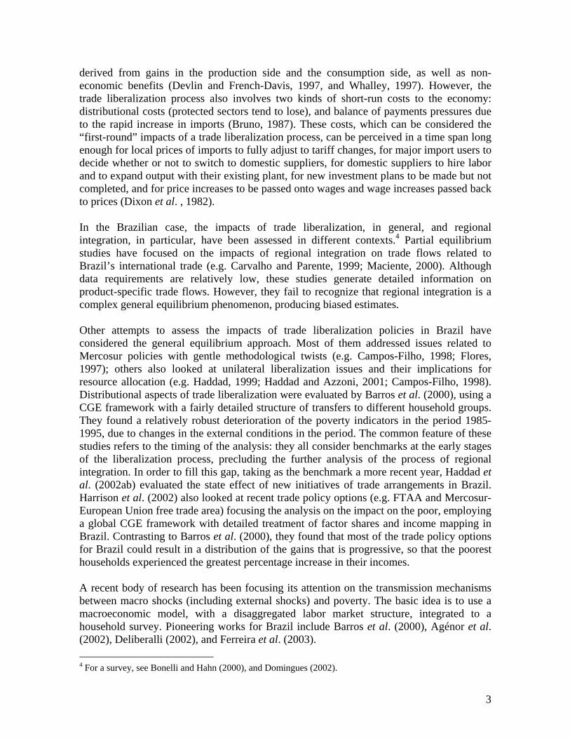
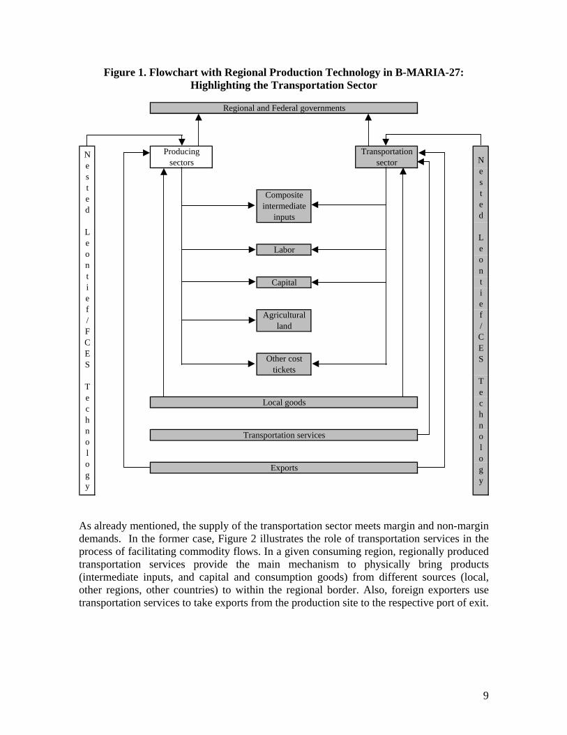
),,,( rqsiθ is a parameter reflecting scale economies to (bulk) transportation. In the calibration of the model, ),,,( rqsiθ is set to one, for every flow. In B-MARIA-27, transportation services (and trade services) are produced by a regional resource-demanding optimizing transportation (trade) sector. A fully specified PPF has to be introduced for the transportation sector, which produces goods consumed directly by users and consumed to facilitate trade, i.e. transportation services are used to ship commodities from the point of production to the point of consumption. The explicit modeling of such transportation services, and the costs of moving products based on origin-destination pairs, represents a major theoretical advance (Isard et al., 1998), although it makes the model structure rather complicated in practice (Bröcker, 1998b). As will be shown, the model is calibrated by taking into account the specific transportation structure cost of each commodity flow, providing spatial price differentiation, which indirectly addresses the issue related to regional transportation infrastructure efficiency. In this sense, space plays a major role. Figure 1 highlights the production technology of a typical regional transport sector in B-MARIA in the broader regional technology. Regional transportation sectors are assumed to operate under constant returns to scale (nested Leontief/CES function), using as inputs composite intermediate goods – a bundle including similar inputs from different sources.9 Locally supplied labor and capital are the primary factors used in the production process. Finally, the regional sector pays net taxes to Regional and Federal governments. The sectoral production serves both domestic and international markets.

9 The Armington assumption is used here.

9

Figure 1. Flowchart with Regional Production Technology in B-MARIA-27: Highlighting the Transportation Sector

Labor

Capital

Other cost tickets

Agricultural land

Regional and Federal governments

Nested Leontief/FCES Technology

Nested Leontief/CES Technology

Local goods

Transportation services

Exports

Producing sectors

Transportation sector

Composite intermediate

inputs

As already mentioned, the supply of the transportation sector meets margin and non-margin demands. In the former case, Figure 2 illustrates the role of transportation services in the process of facilitating commodity flows. In a given consuming region, regionally produced transportation services provide the main mechanism to physically bring products (intermediate inputs, and capital and consumption goods) from different sources (local, other regions, other countries) to within the regional border. Also, foreign exporters use transportation services to take exports from the production site to the respective port of exit.

10

Figure 2. The Role of Transportation Services in B-MARIA-27: Illustrative Flowchart in a Two-Region Integrated Framework

Imports Exports Exports Imports

National border

Region A Region B


Local goods

Local goods

Regi

onal

bor

der


inputs

Composite capital goods

Composite consumption

goods

Interregional trade balance

International trade balance



inputs

Composite capital goods

Composite consumption

goods

The explicit modeling of transportation costs, based on origin-destination flows, which takes into account the spatial structure of the Brazilian economy, creates the capability of integrating the interstate CGE model with a geo-coded transportation network model, enhancing the potential of the framework in understanding the role of infrastructure on regional development. Two options for integration are available, using the linearized version of the model, in which equation (3) 10 becomes:

),,,(*),,,(),,,arg(),,,arg( rqsixrqsirqsiamrqsixm θ+= (2) Considering a fully specified geo-coded transportation network, one can simulate changes in the system, which might affect relative accessibility (e.g. road improvements, investments in new highways). A minimum distance matrix can be calculated ex ante and ex post, and mapped to the interregional CGE model. This mapping includes two stages, one associated with the calibration phase, and another with the simulation phase; both of them are discussed below. 3.4.1. Integration in the Calibration Phase In the interstate CGE model, it is assumed that the locus of production and consumption in each state is located in the state capital. Thus, the relevant distances associated with the flows of commodities from points of production to points of consumption are limited to a matrix of distances between state capitals. Moreover, in order to take into account intrastate transfer costs, it is assumed that trade within the state takes place on an abstract route

10 Equation (A12) in the Appendix.

11

between the capital and a point located at a distance equal to half the implicit radius related to the state area.11 The transport model calculates the minimum interstate time-distances, considering the existing road network in 1997. As Castro et al. (1999) observe, road transportation (i.e. truck) is responsible for the largest share of interstate trade in Brazil, accounting for well over 70% of the total value transported. In Brazil’s North, however, fluvial transportation is particularly important, but the low quality of the services implies equivalent (high) logistic costs. The process of calibration of the B-MARIA-27 model requires information on the transport and trade margins related to each commodity flow. Aggregated information for margins on intersectoral transactions, capital creation, household consumption, and exports are available at the national level. The problem remains to disaggregate this information considering previous spatial disaggregation of commodity flows in the generation of the interstate input-output accounts. Thus, given the available information – interstate/intrastate commodity flows, transport model, matrix of minimum interregional distances and national aggregates for specific margins, the strategy adopted considered the following steps:

1. In an attempt to capture scale effects in transportation – long-haul economies, a tariff function was used to calculate implicit logistic road transport costs in the interstate Brazilian system.12 The function considered was estimated by Castro et al. (1999), for 1994, using freight cost data: 73.0*25.0 disttariff = , where tariff is the road transportation tariff; and dist refers to the distance between two points. This information was then combined with the matrix of minimum interstate distances to generate a matrix of tariffs evaluated for each path. Long-haul effects are clearly perceived in Figure 3, which plots tariffs for different distances within the relevant range for Brazilian interstate trade.

2. By using such transportation structure, one can capture not only the above-

mentioned scale effects, but also relative transfer costs by different origin-destination pairs, which are to be used further on. With that in mind, an index of relative transportation cost was generated. The rows of the tariff matrix were normalized, providing information on differential transportation costs from a given state capital to other state capital, when compared to intrastate costs.

3. The estimates of the various commodity flows at basic values, embedded in the

interstate input-output accounts, were then multiplied by the relevant indices from the normalized tariff matrix. This procedure provides the necessary information to generate a distribution matrix, which considers different spatial-destination weights for commodity flows originating in a given state.

4. Finally, the distribution matrix was applied to national totals, considering

disaggregated national information on margins by different users, maximizing the

11 Given the state area, we assume the state is a circle and calculate the implicit radius. 12 The general form of transport cost functions (…) is either linear or concave with distance. These reflect the usual empirical observations of the relationship between transport costs and haulage distance (McCann, 2001).

12

use of available information. Further balancing was necessary during the calibration of the model.

Figure 3. Estimated Logistic Road Transport Cost Function: (Castro et al., 1999)

0.00

20.00

40.00

60.00

80.00

100.00

120.00

140.00

160.00

025

050

075

010

0012

5015

0017

5020

0022

5025

0027

5030

0032

5035

0037

5040

0042

5045

0047

5050

0052

5055

0057

50

Distance in km

R$/

ton

0.000

0.010

0.020

0.030

0.040

0.050

0.060

R$/

ton/

km

Total cost per ton Cost per ton/km In summary, the calibration strategy adopted here takes into account explicitly, for each origin-destination pair, key elements of the Brazilian integrated interstate economic system, namely: a) the type of trade involved (margins vary according to specific commodity flows); b) the transportation network (distance matters); and c) scale effects in transportation, in the form of long-haul economies. Moreover, the possibility of dealing explicitly with increasing returns to transportation is also introduced in the simulation phase. 3.4.2. Integration in the Simulation Phase When running simulations with B-MARIA-27, one may want to consider changes in the physical transportation network. For instance, one may want to assess the spatial economic effects of an investment in a new highway, expenditures in road improvement, or even the adoption of a toll system, all of which will have direct impacts on transportation costs, either by reducing travel time or by directly increasing out-of-the pocket transfer payments. The challenge becomes one of finding ways to translate such policies into changes in the matrix of minimum interregional time-distances, mimicking potential reductions/increases in the distance between two or more points in space. Such a matrix serves as the basis for integrating the transport model to the interregional CGE model in the simulation phase. One way to integrate both models, in a sequential path, requires the use of either the variable amarg(i,s,q,r) or the parameter ),,,( rqsiθ , in equation (2), as linkage variables. Changes in the matrix of interregional distances are calculated in the transport model, so

13

that an interface with the interregional CGE model is created.13 As in the specification of the margin demand equations the variable distance is only implicitly portrayed in the parameter ),,,( rqsiη , one has to come up with ways in which the information generated by the transport model can be suitably incorporated. Specific transfer rates are present in the model, and changes in them can be easily associated with changes in the matrix of distances. Let us consider, as an example, a two-region economy, consisted of regions A and B. Let us assume the minimum distance through the existing road network is 100km, on a highway that allows the maximum speed of 50 km/h. Thus, traveling 100 km between A and B takes 2 hours. Moreover, the transfer rate for the only commodity flow, from A to B, is 10%. If the government undertakes a project to improve the A-B link, so that, in the operational phase, maximum speed increases to 80 km/h, a change in the transfer rate due to a change in distance – in our example, travel time reduces to one hour and fifteen minutes (time reduction of 37.5%) – may be estimated, using a model-consistent transfer rate function. A new highway project may also be considered, and a more efficient road design may reduce distance between A and B to, say, 75 km. In this sense, if the new road speed limit is also 50 km/h, one can consider a shortening of distance of 25%. Other similar examples apply. In the B-MARIA-27 model, information on transfer (trade and transport) rates is available, and so is information on the relevant distances, enabling estimation of a model-consistent transportation cost function. With that in hand, changes in transfer rates can be estimated and incorporated in the interregional CGE model, as follows. Rearranging equation (3), we have:

),,,(*),,,(),,,(

),,,(),,,( rqsirqsiAMARG

rqsiXrqsiXMARGrqsi ηθ = (3)

with 1),,,( =rqsiθ implying that the left-hand-side becomes the specific transfer (trade or transport) rate. A percentage change in the transfer rate can then be mapped into the technology variable, AMARG(i,s,q,r). Thus, in percentage-change form, amarg(i,s,q,r) becomes the relevant linkage variable, as:

),,,arg(),,,(),,,arg( rqsiamrqsixrqsixm =− (4) The parameter ),,,( rqsiθ can also be used in the simulation phase, especially in sensitivity analysis experiments. Suppose, for instance, that scale effects to transportation appear for a given commodity flow, in a specific path. Changing assumptions on the values of

),,,( rqsiθ allows for addressing this issue in a proper way, instead of relying on hypotheses on the linkage variable, AMARG(i,s,q,r). On this issue, Cukrowski and Fischer (2000), and Mansori (2003) have shown that these spatial implications are considered in the context of international trade, and therefore, increasing returns to transportation should be carefully considered. 13 This procedure assumes one can translate time distance into Euclidean distance. Ideally, one should use a minimum time distance matrix to avoid shortcomings in the process mentioned above.

14

3.5. Closure B-MARIA-27 contains 608,313 equations and 632,256 unknowns. Thus, to close the model, 23,943 variables have to be set exogenously. In order to capture the “first-round” effects of lowering tariffs, the simulations were carried out under a standard short-run closure. A distinction between the short-run and long-run closures relates to the treatment of capital stocks encountered in the standard microeconomic approach to policy adjustments. In the short-run closure, capital stocks are held fixed, while, in the long-run, policy changes are allowed to affect capital stocks. In addition to the assumption of interindustry and interregional immobility of capital, the short-run closure would include fixed regional population and labor supply, fixed regional wage differentials, and fixed national real wage. Regional employment is driven by the assumptions on wage rates, which indirectly determine regional unemployment rates. On the demand side, investment expenditures are fixed exogenously – firms cannot reevaluate their investment decisions in the short-run. Household consumption follows household disposable income, and government consumption, at both regional and federal levels, is fixed (alternatively, the government deficit can be set exogenously, allowing government expenditures to change). Finally, since the model does not present any endogenous-growth-theory-type specification, technology variables are exogenous (Peter, 1997). 3.6. Micro-Macro Integration If one is interested in income distribution analysis (relative poverty), a “pure macro” CGE multi-agent model is sufficient. However, to analyze absolute poverty, a link with a survey is essential. As the households’ responses to economy-wide changes vary across sectors and regions – the growth process is not uniform spatially – the redistribution mechanism will not be homogenous. Increasing focus on welfare, poverty and income distribution calls for strengthened links between macro and household level analysis, so that linkage of macro data and household surveys will contribute to the design of more effective poverty reduction policies and programs.14 The way this link is operational becomes a major research question. First, national/state accounts data and household level information is complementary, though not always consistent. To reconcile the various databases requires special attention to issues related to, for instance: a) year and time of implementation of the survey and construction of national/state core database; b) reference period; c) differences in corrections and adjustment factors used in both household surveys and national/state accounts estimation. In this research, poverty effects of trade reforms are estimated using a top-down approach, following Bussolo (2004). Initially the CGE model calculates the new equilibrium (i.e. new relative prices and quantities for factors and commodities) following a trade shock. Then these prices are transferred to the micro module to estimate a new income distribution, on the latter poverty effects are calculated. No feedback from the micro module to the macro

14 See Agénor et al. (2000).

15

model is explicitly accounted for at this stage. The theoretical background underpinning the calculations in the micro module is detailed in Bussolo (2004). 4. Simulation Results The effects of tariff-barriers decrease are discussed in this section. The B-MARIA-27 model was applied to analyze the “first-round” spatial effects on the Brazilian economy of a uniform 25% decrease in all tariff rates. All exogenous variables were set equal to zero, except the changes in the power of tariffs of tradable goods (agriculture and manufacturing goods), i.e., one plus the tariff rates, which were set such that the percentage change decrease in each tariff rate was 25%.15 In order to capture the role of the transportation infrastructure in the price transmission mechanism of import prices cuts, we introduced the concept of import corridors. In the calibration of the ICGE model, transportation margins on import flows considered only transborder costs, contrary to domestic flows, which, as explained in the previous section, fully considered transportation costs based on origin-destination pairs. In so being, imports were assumed to enter directly the specific consumer markets, facing only transborder costs.16 The implicit assumption was that each state economy constituted the port of entry of its own imports. However, when we observe the spatial distribution of the ports of entry for the state imports, a completely different picture emerges, as some states rely heavily on ports of entry locate outside the state borders (Table 1).17

15 Because of the nature of the database, it should be pointed out that the model deals with changes in the real tariff rates (the ratio of import tax collected over the volume of imports), as opposed to nominal tariff rates. 16 Transborder costs were measured as a weighted average of transportation margins, based on the volume of imports of each state economy and the national totals by specific import flow. 17 Further complication emerges when we consider also the spatial distribution of ports of exit (exports corridors).

Table 1. Regional Distribution of State Imports by Port of Entry* (in %)

AC AP AM PA RO RR TO AL BA CE MA PB PE PI RN SE ES MG RJ SP PR SC RS DF GO MT MSAC 0.4 0.0 0.0 0.0 0.0 0.0 0.0 0.0 0.0 0.0 0.0 0.0 0.0 0.0 0.0 0.0 0.0 0.0 0.0 0.0 0.0 0.0 0.0 0.0 0.0 0.0 0.0AP 0.0 33.9 0.0 0.0 0.0 0.0 0.0 0.0 0.0 0.0 0.0 0.0 0.0 0.0 0.0 0.0 0.0 0.0 0.0 0.0 0.1 0.0 0.0 0.0 0.0 0.0 0.0AM 4.3 0.9 99.5 0.0 38.9 4.0 0.0 0.0 0.0 0.0 0.0 0.0 0.0 0.0 0.0 0.0 0.0 0.0 1.1 0.0 0.0 0.0 0.0 0.0 0.0 4.3 0.0PA 0.0 28.2 0.0 68.0 0.0 0.0 0.0 0.0 0.0 0.0 0.2 0.0 0.0 0.0 0.0 0.0 0.0 0.0 0.0 0.0 0.0 0.0 0.0 0.0 0.0 0.0 0.0RO 0.0 0.0 0.0 0.0 0.5 0.0 0.0 0.0 0.0 0.0 0.0 0.0 0.0 0.0 0.0 0.0 0.0 0.0 0.0 0.0 0.0 0.0 0.0 0.0 0.0 0.0 0.0RR 0.0 0.0 0.0 0.1 0.0 93.7 0.0 0.0 0.0 0.0 0.0 0.0 0.0 0.0 0.0 0.0 0.0 0.0 0.0 0.0 0.0 0.0 0.0 0.0 0.0 0.0 0.1TO 0.0 0.0 0.0 0.0 0.0 0.0 0.0 0.0 0.0 0.0 0.0 0.0 0.0 0.0 0.0 0.0 0.0 0.0 0.0 0.0 0.0 0.0 0.0 0.0 0.0 0.0 0.0AL 0.0 0.0 0.0 0.0 0.0 0.0 0.0 84.5 0.0 0.0 0.0 0.0 0.2 0.0 0.0 0.4 0.0 0.0 0.0 0.0 0.1 0.0 0.0 0.0 0.0 0.0 0.0BA 0.0 0.0 0.0 0.0 0.0 0.0 0.0 8.6 91.6 0.1 0.0 0.4 5.8 10.0 1.4 31.0 0.2 0.0 0.0 0.2 0.0 0.0 0.0 0.4 0.0 0.0 0.0CE 0.0 0.0 0.0 0.1 0.0 0.0 4.2 0.5 0.2 98.1 0.5 22.4 0.1 56.7 4.5 0.0 0.0 0.0 0.0 0.0 0.0 0.0 0.0 0.5 0.0 0.0 0.0MA 0.0 0.0 0.0 25.6 0.0 0.0 0.0 0.0 0.0 0.0 98.9 0.0 0.4 7.2 0.0 0.0 0.0 0.2 0.0 0.0 0.0 0.0 0.0 0.0 0.0 0.0 0.0PB 0.0 0.0 0.0 0.0 0.0 0.0 0.0 0.0 0.6 0.0 0.0 25.9 0.6 2.6 0.3 0.0 0.0 0.0 0.0 0.0 0.0 0.0 0.0 0.0 0.0 0.0 0.0PE 0.0 0.0 0.0 0.1 0.0 0.0 0.0 2.3 0.0 0.1 0.1 33.2 88.0 0.9 16.0 19.9 0.0 0.2 0.0 0.0 0.0 0.0 0.0 0.0 0.0 0.0 0.0PI 0.0 0.0 0.0 0.0 0.0 0.0 0.0 0.0 5.2 0.0 0.0 0.0 0.0 0.0 0.0 0.0 0.0 0.0 0.0 0.0 0.0 0.0 0.0 0.0 0.0 0.0 0.0RN 0.0 0.0 0.0 0.0 0.0 0.0 0.0 0.0 0.0 0.0 0.0 0.0 0.0 0.0 62.9 0.0 0.0 0.0 0.0 0.0 0.0 0.0 0.0 0.0 0.0 0.0 0.0SE 0.0 0.0 0.0 0.0 0.0 0.0 0.0 0.0 0.0 0.0 0.0 0.0 0.0 0.0 0.0 21.4 0.0 0.0 0.0 0.0 0.0 0.0 0.0 0.0 0.0 0.0 0.0ES 0.0 0.0 0.0 1.0 0.0 0.0 0.0 0.0 0.2 0.0 0.1 0.1 0.2 0.1 0.0 0.7 83.2 28.4 0.2 0.0 0.0 0.0 0.0 0.1 16.3 1.0 0.0MG 5.9 0.0 0.0 0.0 0.0 1.3 0.4 0.1 0.3 0.0 0.0 0.0 0.0 0.0 0.0 0.0 0.1 6.9 0.1 0.1 0.1 0.1 0.0 0.2 0.2 1.1 0.0RJ 0.0 0.8 0.2 1.5 23.0 0.0 2.6 0.4 0.0 0.0 0.0 1.4 0.1 0.7 2.4 4.2 5.5 32.0 91.0 0.8 0.4 0.6 0.1 16.5 2.8 0.0 0.3SP 29.4 35.4 0.2 2.5 2.7 1.1 84.0 2.2 0.0 0.7 0.0 12.5 3.5 13.9 10.8 15.5 8.9 25.4 5.1 91.8 6.7 6.9 3.5 35.7 58.2 20.6 9.1PR 60.0 0.0 0.0 0.0 19.6 0.0 6.4 0.6 0.0 0.1 0.0 1.6 0.1 0.1 0.7 6.0 1.0 1.5 0.6 1.5 75.9 17.5 0.5 2.1 17.4 42.1 5.3SC 0.0 0.0 0.0 0.0 0.0 0.0 0.0 0.0 0.0 0.0 0.0 0.0 0.1 0.0 0.0 0.0 0.5 0.8 0.1 0.4 12.3 63.2 1.2 0.3 1.1 4.7 0.4RS 0.0 0.8 0.0 1.1 14.4 0.0 2.4 0.9 0.0 0.9 0.0 2.4 0.8 4.7 1.0 0.7 0.6 4.6 1.6 5.0 3.7 11.5 94.6 0.3 3.7 5.5 9.6DF 0.0 0.0 0.0 0.0 0.0 0.0 0.0 0.0 0.0 0.0 0.0 0.0 0.0 0.0 0.0 0.2 0.0 0.0 0.0 0.0 0.0 0.0 0.0 43.8 0.1 0.0 0.0GO 0.0 0.0 0.0 0.0 0.0 0.0 0.0 0.0 0.9 0.0 0.0 0.0 0.0 0.0 0.0 0.0 0.0 0.0 0.0 0.0 0.0 0.0 0.0 0.0 0.0 0.0 0.0MT 0.0 0.0 0.0 0.0 0.2 0.0 0.0 0.0 0.9 0.0 0.0 0.0 0.0 0.0 0.0 0.0 0.0 0.0 0.0 0.0 0.0 0.0 0.0 0.0 0.0 20.5 0.0MS 0.0 0.0 0.0 0.0 0.7 0.0 0.0 0.0 0.1 0.0 0.0 0.0 0.0 3.1 0.0 0.0 0.0 0.0 0.0 0.1 0.7 0.3 0.0 0.0 0.1 0.0 75.2

Total 100.0 100.0 100.0 100.0 100.0 100.0 100.0 100.0 100.0 100.0 100.0 100.0 100.0 100.0 100.0 100.0 100.0 100.0 100.0 100.0 100.0 100.0 100.0 100.0 100.0 100.0 100.0

Destination

Port

of E

ntry

* State location

17

To deal with this issue, we estimated the implicit transportation costs associated with hypothetical import corridors. We used the information provided in Table 1 and the specific transportation margin rates for each interstate link to estimate the transportation margin rate associated with the 27 hypothetical import corridor. To incorporate these costs in our estimates of the impact of trade liberalization, we then rerun the tariff cut simulation including the import corridors cost through specific shocks in the components of the linkage-variable amarg(i,s,q,r). The shocks were calculated considering the percentage change difference between the effective cost (transborder cost and the cost of shipping the goods from the ports of entry to the place of consumption) and transborder costs only (Figure 4). Two sets of results come out: a) one related to the basic simulation, which does not include the transportation costs associated with the import corridors; and b) one related to the counterfactual simulation, which includes such costs. By comparing the two sets of results, we can assess the role played by the friction of distance and of internal transportation costs in generating an imperfect price transmission mechanism in the country, which, as we will see, potentially hampers the effects of trade liberalization on growth, especially to the more remote regions.

Figure 4. Transborder and Import Corridor Costs: By State (in % of Total Value of Basic Flows of Imported Goods)

0.00

1.00

2.00

3.00

4.00

5.00

6.00

7.00

AC AP AM PA RO RR TO AL BA CE MA PB PE PI RN SE ES MG RJ SP PR SC RS DF GO MT MS

% o

f bas

ic fl

ow

Transborder cost Transborder cost + Import corridor cost 4.1. Basic Results Results of the simulation computed via a four-step Euler procedure, under a short-run closure, are presented below; they show the percentage deviation from the base case (which is the situation without policy changes). The analysis is concentrated on the effects on growth (real GDP/GSP) and household real income. Tables 3 and 4 summarize the simulation results on selected macro and state variables. The real GDP of Brazil is shown to increase with all the states positively affected. Regarding the regional distribution of income, the tariff reduction seems to improve the relative position of São Paulo and Rio de Janeiro, together with some states outside the more

18

dynamic region of the country, even though that is a Pareto-improvement situation (outcome of tariff policy is said to be Pareto superior to outcome without tariff change, as GSP improves in all the regions). At the sectoral level, industry activity results show that, in general, the manufacturing sector is the main loser from the tariff cut. However, when we take into account the import corridors costs, a different picture emerges. The counterfactual simulation exercise considers an increase in the transportation cost in the Brazilian interstate system associated with import corridors. According to the model structure, this represents a less intensive use of margins, i.e. the use of transportation services per unit of output is increased, implying a direct increase in the output of the transportation sector. As shipments become more resource-intensive, labor and capital are drawn from other sectors generating excess demand of primary factors in the economic system. This creates an upward pressure on wages and capital rentals, which are passed on in the form of higher prices. Moreover, higher transport costs increase the price of composite commodities, with negative implications for real regional income: in this cost-competitiveness approach, firms become less competitive – as production costs go up (inputs are more costly); investors foresee potential lower returns – as the cost of producing capital also increases; and households decreases their real income, envisaging lower consumption possibilities. Lower income generates lower domestic demand, while decreases in the competitiveness of national products hampers external demand. This creates room for decreasing firms’ output – directed for both domestic and international markets – which requires less inputs and primary factors. Decreasing demand puts pressure on the factor markets for price decreases, with a concomitant expectation that the prices of domestic goods would decrease. Second-order prices changes go in both directions – increase and decrease. The net effect is determined by the relative strength of the countervailing forces. Comparison of the two columns of Table 3 reveals some of these consequences. First, the effects of unilateral trade liberalization on growth and welfare is weakened, as real GDP and equivalent variation does not grow as fast. Second, high transportation costs also appear to harm the country’s competitiveness, and real household income and consumption. At the sectoral level, there seems to be a shift towards the production of transportation services, as expected. As resources are scarce, the additional production of transportation services is performed at the expense of other sectoral output, especially from sectors producing tradable goods, which face stronger competition from foreign products. Regarding the spatial effects (Table 4), there appears to be a spatial shift of the relative benefits of tariff cuts towards the coastal states, where a large part of the ports locate. This movement can be perceived through the analysis of Figures 5A and 5B (south-eastward movement of warm colors).18

18 In the reading of the maps, hereafter, warm colors (orange and green) represent values above the average, in terms of standard deviations; cold colors (blue) represent values below the average, also in terms of standard deviations; warmer/colder colors represent outliers.

19

Table 3. Aggregate Results: Selected Variables (in percentage-change)

Import corridors costs Non-included Included Activity level Agriculture 0.0252 0.0210 Manufacturing -0.0112 -0.0195 Utilities 0.0155 0.0155 Construction 0.0017 0.0022 Trade 0.0419 0.0418 Financial institutions 0.0460 0.0435 Public administration 0.0132 0.0125 Transportation and other services 0.0597 0.0827 Prices Investment price index -0.5836 -0.5336 Consumer price index -0.4395 -0.3708 Exports price index -0.4838 -0.4453 Regional government demand price index -0.4472 -0.3829 Federal government demand price index -0.4410 -0.3711 GDP price index, expenditure side -0.4997 -0.4321 Primary factors Aggregate payments to capital -0.3030 -0.2303 Aggregate payments to labor -0.3817 -0.3043 Aggregate employment, wage bill weights 0.0580 0.0668 Aggregate demand Real household consumption 0.0521 0.0517 Export volume 1.0028 0.9218 Aggregate indicators Equivalent variation – total (change in $) 1670.74 1667.98 Real GDP 0.0202 0.0110

20

Table 4. State Results

Import corridors costs Non-included Included

Acre 0.0003 -0.0039 Amapá 0.0185 -0.0037 Amazonas 0.0433 -0.0386 Pará 0.0125 0.0054 Rondônia 0.0157 -0.0100 Roraima 0.0603 0.0605 Tocantins 0.0001 -0.0067 Alagoas 0.0167 0.0105 Bahia 0.0133 0.0100 Ceará 0.0069 0.0009 Maranhão 0.0601 0.0463 Paraíba 0.0271 0.0110 Pernambuco 0.0061 0.0026 Piauí 0.0073 -0.0093 Rio Grande do Norte 0.0040 -0.0006 Sergipe 0.0021 -0.0023 Espírito Santo 0.0169 -0.0002 Minas Gerais 0.0010 -0.0202 Rio de Janeiro 0.0229 0.0175 São Paulo 0.0292 0.0230 Paraná 0.0088 0.0047 Santa Catarina 0.0059 -0.0007 Rio Grande do Sul 0.0147 0.0078 Distrito Federal 0.0354 0.0403 Goiás 0.0064 -0.0019 Mato Grosso 0.0311 0.0259 Mato Grosso do Sul 0.0088 0.0082

21

Figure 5. State Effects on Regional Growth (Real GSP): With and Without Import Corridors Costs

(standard deviation)

A. Non-included B. Included

4.2. The Effects of Import Corridors Costs It has been argued that, given the intrinsic uncertainty in the shock magnitudes and parameter values, sensitivity tests are an important next step in the more formal evaluation of the robustness of (interregional) CGE analysis and the fight against the “black-box syndrome.” However, some important points should be addressed in order to have a better understanding of the sensitivity of the models’ results. In similar fashion to the fields of influence approach for input-output models developed by Sonis and Hewings (1989), attention needs to be directed to the most important synergetic interactions in a CGE model. It is important to try to assemble information on the parameters, shocks and database flows, for example, that are the analytically most important in generating the model outcomes, in order to direct efforts to a more detailed investigation.19 In order to address this issue, in the context of our counterfactual simulation, we proceeded with a thorough decomposition of the results considering the role played by the shocks associated with specific macro-regional import corridors. In other words, we explicitly considered the role played by five groups of transportation links (between ports of entry and macro-regional state markets) in generating the model’s results. For each group of transportation links, we calculated its contribution to the total outcome, considering different dimensions of regional policy. Impacts on regional efficiency and regional household income were considered. We looked at the effects on regional efficiency, through the differential impacts on GSP growth. Moreover, we considered the differential impacts on household wealth, looking at the specific state results for household real income. The analysis will focus on the decomposition of the net effects associated with the import corridors costs, i.e. we attempt to identify the sources of market imperfections that affect

19 See Domingues et al. (2004).

22

state performance related to trade liberalization. Tables 5 and 6 present the results for the five major groups of import corridors, showing their contributions to the specific deviations of the policy basic outcome. Regarding regional performance in terms of real GSP growth, it is noteworthy the negative impact high transportation costs impose to the regions. Specific import corridors affect the destination regional economies more intensively, as expected. Given the spatial interaction of the Brazilian interstate system, states outside the macro-region under consideration are also affected. Overall, states more remotely located – both in terms of distance from the central position20 or access to ports – are more adversely affected. Spatial positive impacts can be perceived as some regions might be positively impacted through re-orientation of trade flows (trade diversion), as relative accessibility changes in the system. Figures 6A-6E highlight the states that present stronger negative impacts due to the presence of costs related to specific import corridors; Figure 6F shows the overall picture. Regional household disposable income is also hampered by high transportation costs. However, there appears a strong relationship between the specific import corridors and the income of the residents of the macro-region suffering from spatial imperfect markets. In other words, resident households income are negatively affected by high transportation costs associated to the channels of distribution of imports to the region. Households elsewhere perceive an increment in their income, as the relative competitive advantage of outside states increases. This result has strong implications for understanding transmission mechanisms that relate trade liberalization and poverty. As one thinks about the effects of trade on poverty and the spatial distribution of income, the role of internal transportation barriers should not be neglected, especially for peripheral regions, lacking the appropriate infrastructure for trade facilitation through proper distribution mechanisms.

20 Central position defined not geographically, but in terms of the locus of productive activity or purchasing power (see Haddad and Azzoni, 2001).

23

Table 5. Decomposition of Net Effects of Transportation Costs on the Impacts of Tariff Reductions on Regional Growth (Real GSP): By Import Corridors

(in percentage change)

Import Corridors North Northeast Southeast South Center-west Total

Acre -0.0017 -0.0001 -0.0021 -0.0003 -0.0001 -0.0043 Amapá -0.0201 -0.0001 -0.0017 -0.0003 -0.0001 -0.0222 Amazonas -0.0827 0.0000 0.0007 0.0001 0.0000 -0.0819 Pará -0.0046 -0.0003 -0.0019 -0.0003 -0.0001 -0.0070 Rondônia -0.0242 -0.0001 -0.0011 -0.0003 0.0000 -0.0257 Roraima -0.0004 0.0000 0.0005 0.0001 0.0000 0.0001 Tocantins -0.0022 -0.0004 -0.0035 -0.0004 -0.0003 -0.0067 Alagoas -0.0014 -0.0020 -0.0023 -0.0004 -0.0001 -0.0062 Bahia -0.0001 -0.0027 -0.0003 0.0000 0.0000 -0.0033 Ceará -0.0015 -0.0021 -0.0020 -0.0004 -0.0001 -0.0060 Maranhão -0.0034 -0.0020 -0.0071 -0.0010 -0.0002 -0.0137 Paraíba -0.0012 -0.0120 -0.0025 -0.0004 -0.0001 -0.0161 Pernambuco -0.0008 -0.0014 -0.0011 -0.0002 0.0000 -0.0035 Piauí -0.0029 -0.0072 -0.0056 -0.0008 -0.0002 -0.0166 Rio Grande do Norte -0.0007 -0.0018 -0.0017 -0.0003 -0.0001 -0.0046 Sergipe -0.0005 -0.0022 -0.0014 -0.0003 -0.0001 -0.0044 Espírito Santo -0.0003 -0.0001 -0.0165 -0.0001 0.0000 -0.0171 Minas Gerais -0.0014 -0.0003 -0.0190 -0.0004 -0.0001 -0.0212 Rio de Janeiro 0.0001 0.0000 -0.0055 0.0000 0.0000 -0.0055 São Paulo -0.0005 -0.0001 -0.0054 -0.0001 0.0000 -0.0062 Paraná -0.0008 -0.0001 -0.0017 -0.0014 -0.0001 -0.0041 Santa Catarina -0.0007 -0.0001 -0.0016 -0.0041 -0.0001 -0.0066 Rio Grande do Sul -0.0003 -0.0001 -0.0006 -0.0059 0.0000 -0.0069 Distrito Federal 0.0020 0.0002 0.0027 0.0004 -0.0004 0.0049 Goiás -0.0014 -0.0003 -0.0031 -0.0004 -0.0031 -0.0082 Mato Grosso -0.0019 0.0000 -0.0017 -0.0003 -0.0012 -0.0052 Mato Grosso do Sul -0.0002 0.0000 0.0000 -0.0001 -0.0004 -0.0006 North -0.0476 -0.0001 -0.0005 -0.0001 0.0000 -0.0483 Northeast -0.0009 -0.0029 -0.0015 -0.0002 -0.0001 -0.0055 Southeast -0.0005 -0.0001 -0.0078 -0.0001 0.0000 -0.0086 South -0.0005 -0.0001 -0.0012 -0.0040 -0.0001 -0.0059 Center-west -0.0001 0.0000 -0.0002 0.0000 -0.0013 -0.0016 Brazil -0.0028 -0.0004 -0.0051 -0.0008 -0.0001 -0.0092

24

Figure 6. Decomposition of Net Effects of Transportation Costs on the Impacts of Tariff Reductions on Regional Growth (Real GSP): By Import Corridors


A. North B. Northeast

C. Southeast D. South

E. Center-west F. Total

25

Table 6. Decomposition of Net Effects of Transportation Costs on the Impacts of Tariff Reductions on Regional Household Disposable Income: By Import Corridors

(in percentage change)

Import Corridors North Northeast Southeast South Center-west Total

Acre -0.0011 0.0005 0.0069 0.0011 0.0001 0.0074 Amapá -0.0234 0.0002 0.0041 0.0007 0.0001 -0.0183 Amazonas -0.1240 0.0004 0.0050 0.0009 0.0002 -0.1176 Pará -0.0112 0.0004 0.0060 0.0010 0.0000 -0.0038 Rondônia -0.0815 0.0004 0.0063 0.0010 0.0001 -0.0738 Roraima 0.0012 0.0003 0.0059 0.0009 0.0001 0.0085 Tocantins 0.0025 0.0006 0.0063 0.0009 -0.0001 0.0103 Alagoas 0.0042 -0.0035 0.0071 0.0011 0.0002 0.0091 Bahia 0.0038 -0.0041 0.0068 0.0010 0.0001 0.0077 Ceará 0.0032 -0.0035 0.0084 0.0013 0.0002 0.0097 Maranhão 0.0050 -0.0051 0.0094 0.0014 0.0002 0.0110 Paraíba 0.0038 -0.0399 0.0081 0.0011 0.0002 -0.0267 Pernambuco 0.0036 0.0000 0.0063 0.0009 0.0001 0.0109 Piauí 0.0041 -0.0136 0.0074 0.0012 0.0002 -0.0007 Rio Grande do Norte 0.0037 -0.0038 0.0069 0.0011 0.0002 0.0081 Sergipe 0.0022 -0.0073 0.0029 0.0006 0.0001 -0.0015 Espírito Santo 0.0049 0.0006 -0.0205 0.0014 0.0002 -0.0133 Minas Gerais 0.0046 0.0006 -0.0265 0.0013 0.0002 -0.0197 Rio de Janeiro 0.0030 0.0003 -0.0026 0.0009 0.0001 0.0017 São Paulo 0.0037 0.0004 0.0026 0.0010 0.0001 0.0079 Paraná 0.0011 0.0003 -0.0003 -0.0016 -0.0001 -0.0005 Santa Catarina 0.0036 0.0005 0.0049 -0.0062 0.0002 0.0029 Rio Grande do Sul 0.0038 0.0004 0.0081 -0.0096 0.0002 0.0030 Distrito Federal 0.0055 0.0006 0.0082 0.0013 -0.0003 0.0153 Goiás 0.0036 0.0005 0.0016 0.0009 -0.0058 0.0008 Mato Grosso 0.0016 0.0006 0.0079 0.0011 -0.0005 0.0106 Mato Grosso do Sul 0.0037 0.0004 0.0086 0.0012 -0.0003 0.0137 Brazil 0.0007 -0.0008 -0.0002 -0.0001 0.0000 -0.0004

26

Figure 7. Decomposition of Net Effects of Transportation Costs on the Impacts of Tariff Reductions on Regional Household Disposable Income: By Import Corridors





27

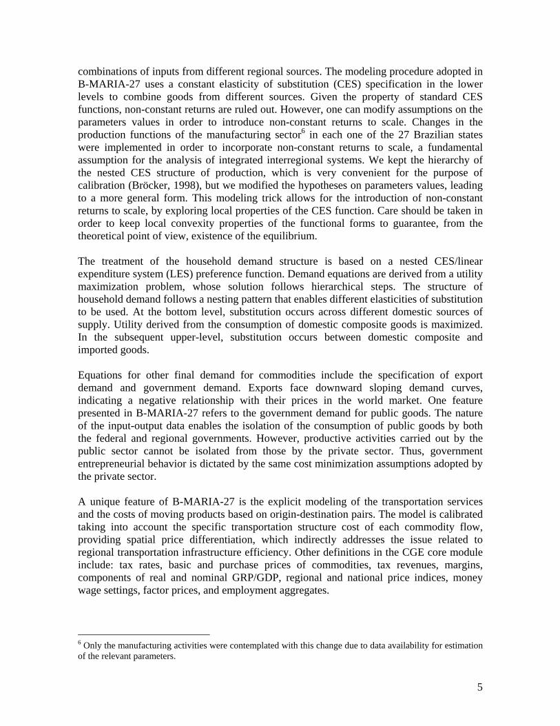
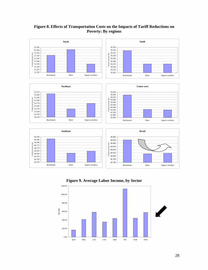
4.3. Effects on Poverty In this section, we have considered the above-mentioned simulation results in conjunction with a non-behavioral micro-simulation module based on households survey data, in order to address more properly issues relating trade and regional poverty.21 As Bussolo (2004) points out, the CGE model has the main advantage of being a counterfactual analysis tool, so that it can generate price effects that are directly and unequivocally linked to a trade reform. The changes in relative factor prices (particularly between labor and capital remunerations) and relative goods price (regional CPIs) were linked to the household survey and new income distributions were generated. By combining the micro data and the CGE results, the aggregate results from the CGE could be mapped to the detailed information available in the household survey and a much more complex and useful analysis of the poverty impact was provided.22 We have seen that further trade liberalization has strong implications for the spatial distribution of output and income in the Brazilian case. By taking into account the various regional dimensions of households’ income and expenditures patterns, with detailed information from PNAD, even more enlightening insights can be captured from the analysis. This will enable us to better assess the role of transportation policies as compensatory regional policies. Figure 8 presents the results of the simulations considering the poverty effects. Regional poverty lines (Rocha, 2003) were used in order to estimate the percentage of the population in each state/region living under in poverty. Data from PNAD 1996 were compiled and reconciled with the CGE database, before running the non-behavioral micro-simulation. In addition to the benchmark estimates, two sets of results were generated. The first refers to the basic simulation, which does not include the transportation costs associated with the import corridors; the second refers to the counterfactual simulation, which includes such costs. There appears a “U-shaped” pattern in which, for the coastal regions (Northeast, Southeast and South), and for the country as a whole, poverty seems to increase when transportation costs are properly considered. On the other hand, for the more internal regions (North and Center-west), the effect of transport corridors affects positively poverty reduction, when compared to the basic simulation. Two effects appear to be acting as the main driving forces of the results. First, there appears a competitiveness (negative) effect, which tends to hamper poverty and prevail in the areas closer to the ports of entry. Second, a composition effect: as the transportation sector is a better paying sector (Figure 9), a shift towards it helps to reduce poverty, as long as employment does not fall sharply.23

21 Bussolo (2004). 22 The main information from the CGE results refer to sector and state-specific labor and capital income, employment, household transfers, and regional prices. 23 The complementary performance of the construction sector, which employs many workers, acts in such direction.

28

Figure 8. Effects of Transportation Costs on the Impacts of Tariff Reductions on Poverty: By regions

North

51.52051.52551.53051.53551.54051.54551.55051.55551.56051.565

Benchmark Basic Import corridors

% b

elow

pov

erty

line

Northeast

53.12053.13053.14053.15053.16053.17053.18053.19053.20053.210


% b

elow

pov

erty

line

Southeast

44.14544.15044.15544.16044.16544.17044.17544.18044.18544.190


% b

elow

pov

erty

line

South

39.24039.25039.26039.27039.28039.29039.30039.31039.32039.330


% b

elow

pov

erty

line

Center-west

45.46045.48045.50045.52045.54045.56045.58045.60045.62045.64045.660


% b

elow

pov

erty

line

Brazil

46.78046.790

46.80046.81046.82046.830

46.84046.85046.860


% b

elow

pov

erty

line

Figure 9. Average Labor Income, by Sector

0.00

200.00

400.00

600.00

800.00

1000.00

1200.00

AGP MFG UTI CNT TRD FIN PUB TRN

R$

1996

29

Epilogue: The Holistic Picture In this paper, we attempted to elucidate one of the mechanisms that link own trade liberalization and subsequent growth and regional inequality. By considering explicitly the distribution costs of imports from the ports of entry to the place of consumption, we have shown that high internal transportation costs impose spatial impediments for the internal transmission of the potential benefits of trade liberalization, hampering the more remote regions in terms of growth. However, a composition-effect may benefit some areas in those regions in terms of poverty reduction, even though the overall national effect would be non-desirable. We have analyzed only one side of the token. It is agreed that constraints towards export expansion can also be perceived as a further barrier to link trade liberalization and growth. As a topic for further investigation, the role of export corridors must be considered in order to grasp the holistic picture. To tackle this issue, we proceeded further by also estimating the implicit transportation costs associated with hypothetical export corridors, in a similar fashion as the procedure for estimating implicit import corridors. Figure 10 presents the results for the five major groups of import and export corridors, showing their joint contributions to the specific deviations of the policy basic outcome, in terms of GDP growth. There appears clearly a “coastal effect”, characterizing two spatial regimes in the Brazilian economy. In other words, the effects of trade liberalization are further hindered by additional spatial impediments in the form of higher transportation costs associated with the transfer of goods form the points of production to the ports of exit.

30

Figure 10. Decomposition of Net Effects of Transportation Costs on the Impacts of Tariff Reductions on Regional Growth (Real GSP): By Import/Export Corridors




31

References

Agénor, P. R., Fernandes, R. and Haddad, E. (2002). Analyzing the Impact of Adjustment Policies on the Poor: An IMMPA Framework for Brazil. Work in progress, The World Bank and University of Sao Paulo.

Baer, W. and Maloney, W. (1997). Neoliberalism and Income Distribution in Latin America. World Development, vol. 25, no. 3, pp. 311-327.

Baer, W., Haddad, E. A. and Hewings, G. J. D. (1998). The Regional Impact pf Neo-Liberal Policies in Brazil. Revista de Economia Aplicada, vol. 2, n. 2.

Barros, R. P., Corseuil C. H., and Cury S. (2000). Abertura Comercial e Liberalização do Fluxo de Capitais no Brasil: Impactos sobre a Pobreza e Desigualdade. In Henriques, R. (org.). Desigualdade e pobreza no Brasil. Rio de Janeiro: IPEA.

Bilgic, A., King, S., Lusby, A. and Schreiner, D. F. (2002). “Estimates of U.S. Regional Commodity Trade Elasticities”. Journal of Regional Analysis and Policy, 32(2).

Bonelli, R. and Hahn, L. (2000). Survey of Recent Studies on Brazilian Trade Relations. IPEA, Discussion Paper #708, Rio de Janeiro (in Portuguese).

Bröcker, J. (1998). “Spatial Effects of Transport Infrastructure: The Role of Market Structure”. Diskussionbeiträge aus dem Institut für Wirtschaft und Verkehr, 5/98.

Bruno, M. (1987). Opening-Up: Liberalization with Stabilization. In: Eds. R. Dornbusch and L. Helmers, The Open Economy: Tools for Policymakers in Developing Countries, Oxford University Press.

Bussolo, M. (2004). An Empirical Evaluation of the Economic and Poverty Impacts of the Central America Free Trade Agreement For Nicaragua, mimeo.

Campos-Filho, L. (1998). Unilateral Liberalisation and Mercosul: Implications for Resource Allocation. Revista Brasileira de Economia, vol. 52, no. 4, pp. 601-636.

Carvalho, A. and Parente, A. (1999). Trade Impacts of FTAA. IPEA, Discussion Paper #635, Brasilia (in Portuguese).

Cukrowski, J. e Fischer, M. M. (2000). “Theory of Comparative Advantage: Do Transportation Costs Matter?”, Journal of Regional Science, 40(2): 311-322.

Deliberalli, P. P. (2002). Impacto da Educação sobre a Pobreza e Distribuição de Renda no Brasil. Unpublished Master Thesis, University of São Paulo.

Devlin, R. and French-Davis, R. (1997). Towards an Evaluation of Regional Integration in Latin America in the 1990s. Inter-American Development Bank, Integration, Trade and Hemispheric Issues Division, Occasional Paper #1.

Dixon, P. D. e Parmenter, B. R. (1996). “Computable General Equilibrium Modeling for Policy Analysis and Forecasting”. In: H. M. Amman, D. A. Kendrick e J. Rust (Eds.), Handbook of Computational Economics, 1: 3-85, Amsterdam, Elsevier.

Dixon, P. B., Parmenter, B. R., Sutton, J. and Vincent, D. P. (1982). ORANI: A Multisectoral Model Of The Australian Economy. North-Holland, Amsterdam.

32

Domingues, E. P. (2002). Dimensão Regional e Setorial da Integração Brasileira na Área de Livre Comércio das Américas. Unpublished Ph.D. Thesis, University of São Paulo.

Domingues, E. P., Haddad, E. A. and Hewings, G. J. D. (2004). “Sensitivity Analysis in Applied General Equilibrium Models: an Empirical Assessment for MERCOSUR Free Trade Areas Agreements.” Discussion Paper 04-T-4, Regional Economics Applications Laboratory, University of Illinois, Urbana.

Ferreira, H. G. F., Leite, P. G., Silva, L. P. and Picchetti, P. (2003). Aggregate Shocks and Income Distribution: Can Macro-Micro Models Help Identifying Winners and Losers from a Devaluation? Mimeo, the World Bank.

Flores Jr., R. G. (1997). The Gains from Mercosul: A General Equilibrium, Imperfect Competition Evaluation. Journal of Policy Modeling, vol. 19, no. 1, pp. 1-18.

Guilhoto, J.J.M., M.M. Hasegawa, e R.L. Lopes (2002). “A Estrutura Teórica do Modelo Inter-regional para a Economia Brasileira – MIBRA”. Anais do II Encontro de Estudos Regionais e Urbanos. São Paulo, São Paulo, 25 a 26 de outubro.

Haddad, E. A. (1999). Regional Inequality and Structural Changes: Lessons from the Brazilian Experience. Ashgate, Aldershot.

Haddad, E. A. and Azzoni, C. R. (2001). Trade and Location: Geographical Shifts in the Brazilian Economic Structure. In: Eds. J. J. M. Guilhoto and G. J. D. Hewings, Structure and Structural Change in the Brazilian Economy, Ashgate, Aldershot.

Haddad, E. A., Azzoni, C. R., Domingues, E. P. and Perobelli, F. S. (2002). Macroeconomia dos Estados e Matriz Interestadual de Insumo-Produto. Revista de Economia Aplicada, vol. 6, n. 4, pp. 875-895.

Haddad, E. A., Domingues, E. P. and Perobelli, F. S. (2002a). Regional Effects of Economic Integration: The Case of Brazil. Journal of Policy Modeling, vol. 24, pp. 453-482.

Haddad, E. A., Domingues, E. P. and Perobelli, F. S. (2002b). Regional Aspects of Brazil’s Trade Policy. INTAL-ITD-STA Occasional Paper 18, IADB, Washington, D.C..

Haddad, E. A. and Hewings, G. J. D. (1997). The Theoretical Specification of B-MARIA. Discussion Paper REAL 97-T-5, Regional Economics Applications Laboratory, University of Illinois at Urbana-Champaign, November.

Harrison, G. W., Rutherford, T. F., Tarr, D. G., and Gurgel, A. (2002). Regional, Multiregional and Unilateral Trade Policies of MERCOSUR for Growth and Poverty Reduction in Brazil. XXX Encontro Nacional de Economia, Nova Friburgo, RJ.

Horridge, J. M., Parmenter, B. R. and Pearson, K. R. (1993). ORANI-F: A General Equilibrium Model of the Australian Economy. Economic and financial Computing, vol. 3, n. 2, Summer.

Isard, W., Azis, I. J., Drennan, M. P., Miller, R. E., Saltzman, S. and Thorbecke, E. (1998). Methods of Interregional and Regional Analysis, Aldershot, Ashgate.

Maciente, A. (2000). Comparative Analysis of FTAA and a Free Trade Agreement Between Mercosul and European Union. Unpublished Master Thesis, University of São Paulo (in Portuguese).

33

Mansori, K. F. (2003). “The Geographic Effects of Trade Liberalization with Increasing Returns in Transportation”. Journal of Regional Science, 43(2): 249-268.

McCann, P. (2001). Urban and Regional Economics. Oxford University Press.

Peter, M. W., Horridge, M., Meagher, G. A., Naqvi, F. e Parmenter, B. R. (1996). “The Theoretical Structure Of MONASH-MRF”. Preliminary Working Paper no. OP-85, IMPACT Project, Monash University, Clayton, April.

Rocha, S. (2003). Pobreza: Afinal, de que se trata?. FGV, Rio de Janeiro.

Sonis, M. e Hewings, G. J. D. (1989). “Error and Sensitivity Input-Output Analysis: A New Approach”. In: R. E. Miller, K. R. Polenske, e A. Z. Rose, (Eds.). Frontiers of Input-Output Analysis. New York, Oxford University Press.

Venables, A. J. (1998). The Assessment: Trade and Location. Oxford Review of Economic Policy, vol. 14, no. 2, Summer.

Whalley, J. (1997). Why do Countries Seek Trade Agreements? In: Ed. J. A. Frankel, The Regionalization of the World Economy, NBER, The University of Chicago Press, Chicago.

34

Appendix A The functional forms of the main groups of equations of the interstate CGE core are presented in this Appendix together with the definition of the main groups of variables, parameters and coefficients. The notational convention uses uppercase letters to represent the levels of the variables and lowercase for their percentage-change representation. Superscripts (u), u = 0, 1j, 2j, 3, 4, 5, 6, refer, respectively, to output (0) and to the six different regional-specific users of the products identified in the model: producers in sector j (1j), investors in sector j (2j), households (3), purchasers of exports (4), regional governments (5) and the Federal government (6); the second superscript identifies the domestic region where the user is located. Inputs are identified by two subscripts: the first takes the values 1, ..., g, for commodities, g + 1, for primary factors, and g + 2, for “other costs” (basically, taxes and subsidies on production); the second subscript identifies the source of the input, being it from domestic region b (1b) or imported (2), or coming from labor (1), capital (2) or land (3). The symbol (•) is employed to indicate a sum over an index. Equations (A1) Substitution between products from different regional domestic sources

∑∈

• •−−=*

)))(),(,1,(/)),(,1,((( )())1((

)())1((

)()(

)())1((

)())1((

Sl

ruli

rubi

rui

rui

rubi pruiVruliVpxx σ

Rrhjkkjuqbgi ,...,1 ;,...,1 and 2 and 1for )( and 3)( ;,...,1 ;,...,1 ====== (A2) Substitution between domestic and imported products

∑•=

• •−−=2,1

)()(

)()(

)()(

)()(

)()( )))(),(,,(/)),(,,(((

l

ruil

ruis

rui

rui

ruis pruiVruliVpxx σ

Rrhjkkjusgi ,...,1 ;,...,1 and 2 e 1for )( and 3)( ;2 and 1 ;,...,1 ====•== (A3) Substitution between labor, capital and land

})))(),1(,,1(/)),1(,,1((-

{

3,2,1

)1(),1(

)1(),1(

)1(),1(

)1(),1(

)1()1(

)1()1(

)1(),1(

)1(),1(

)1(),1(

∑=

++

+++++++

+++

+−=−

•

•

l

rjlg

rjlg

rjsg

rjsg

rjg

rjg

rjsg

rjsg

rjsg

aprjgVrjlgV

apxax σα

Rrshj ,...,1 ;3 and 2 ,1 ;,...,1 ===

35

(A4) Intermediate and investment demands for composites commodities and primary factors

,...,1 ;1 then 2 if

21 then )(1 if

1,..., and 2 , 1for )( )()(

)()()(

)()(

Rr,...,g ij) (u,...,giju

hjkkjuazx rui

rurui

rui

===

+==

===+= •• µ

(A5) Household demands for composite commodities

∑∈

••••••

••

+−++

=+•

Gj

ri

ri

rri

rj

rri

ri

ri

rri

r

ri

ri

xpQPCxpQP

xpriV

i))(()(

))(),3(,,()3()(

)3()(

)3()()()(

)3()(

)3()(

)3()(

)3()(

)3()(

)(γβγ

Rrgi ,...,1 ;,,1 == K (A6) Composition of output by industries

))),,(/),,((( )0()1(

)0()1(

)0()1()0()1( ∑

∈

•−+=Gt

rt

ri

rjrjrji prjYrjtYpzx σ

Rrhj ,...,1 g;1,...,i ;,...,1 ===

(A7) Indirect tax rates

Rrhjkkju

tqbbsgiffffrusit rui

uii

,...,1 ,...,1 ;2 ,1for )( and (6) (5), ),4(),3()(

,...,1 ;,...,1for 2,1 ;,...,1 ,))(,,,( )()(

)()()()(

====

====+++= ττ ττττ

(A8) Purchasers’ prices related to basic prices, margins (transportation costs) and taxes

Rrqbbshjkkj

ugi

r)p)M(m,i,s,(u

rusitprusiTrusiBprusiV

Gm

)r()(m

isT

ruis

,...,1 ,...,1for 2 ,1 ;,...,1 and 2 ,1for )( and

(6) (5), ),4( ),3()( ;,...,1

,,

)),,,,()()),(,,,()),(,,(()),(,,(

01

)0()(

)()(

=====

==

+

++=

∑

∑

∈

∈

τττ

36

(A9) Foreign demands (exports) for domestic goods

Rrqbbs,...,g ifpepfqx ris

ris

ris

ris

ris ,...,1;,...,1for 2 ,1 ; 1 , )()( )4(

)()4()()(

)4()(

)4()( ====−−=− η

(A10) Regional governments demands

R1,...,r ;,...,1for 2,1 ;,...,1 )5()5()5()(

)3()(

)5()( ====+++= •• qbbsgifffxx rr

isrr

is (A11) Regional governments demands

R1,...,r ;,...,1for 2,1 ;,...,1 )6()6()6()(

)3()(

)6()( ====+++= •

•• qbbsgifffxx rris

ris

(A12) Margins demands for domestic goods

ruism

ruis

ruis

ruism axx ))((

)1()()(

)()(

))(()1( += θ

Rrrbbshj

kkjrbbugim

,...,1;,...,1for 2 ,1 ;,...,1

;2 ,1for )( and (5) ,,...,1for )4(),3()(;,...,1,

====

====

(A13) Demand equals supply for regional domestic commodities

RrglxrusilM

xrulBxrjlY

Gi Ss Uu

ruisl

Hj Uu

rul

rjl

,...,1 ;,...,1 )),(,,,(

)),(,1,(),,(

))(()1(

)()1(

)0()1(

==+

=

∑∑∑

∑ ∑

∈ ∈ ∈

∈ ∈

(A14) Regional industry revenue equals industry costs

RrhjprjslVaprjlYGl Gl Ss

rjls

rl

rl ,...,1 ;,...,1 ,))(),1(,,())(,,(

*

)1()(

)0()1(

)0()1( ===+∑ ∑∑

∈ ∈ ∈

(A15) Basic price of imported commodities

gitepp iwii ,...,1 ,)0(

))2(()())2((

)0())2(( =+−=

37

(A16) Cost of constructing units of capital for regional industries

RrhjaprjsiVaprjVGi Ss

rjis

rjis

rjk

rjk ,...,1 ;,...,1 ,))(),2(,,())(),2(,,( )2(

)()2(

)()1(

)()1(

)( ==+=− ∑∑∈ ∈

••

(A17) Investment behavior

Rrhjfxz rjk

rjg

rj ,...,1 ;,...,1 ,100 )2()(

)1()2,1(

)2( ==+= + (A18) Capital stock in period T+1 – comparative statics

Rrhjxx rjg

rjg ,...,1 ;,...,1 )1( )1(

)2,1()1(

)2,1( === ++ (A19) Definition of rates of return to capital

RrhjppQr rjk

rjg

rj

rj ,...,1 ;,...,1 ),( )1(

)()1(

)2,1()()( ==−= + (A20) Relation between capital growth and rates of return

Rrhjfxxr rk

rg

rjg

rj

rj ,...,1 ;,...,1 ,)( )(

)()2,1(

)1()2,1()()( ==+−=− •

++εω Other definitions in the CGE core include: revenue from indirect taxes, import volume of commodities, components of regional/national GDP, regional/national price indices, wage settings, definitions of factor prices, and employment aggregates.

38

Variables

Variable Index ranges Description Demand by user (u) in region r for good or primary factor (is)

ruisx )(

)(

(u) = (3), (4), (5), (6) and (kj) for k = 1, 2 and j = 1,…,h; if (u) = (1j) then i = 1,…,g + 2; if (u) ≠ (1j) then i = 1,…,g; s = 1b, 2 for b = 1,…,q; and i = 1,…,g ands = 1, 2, 3 for i = g+1 r = 1,…,R

ruisp )(

)( (u) = (3), (4), (5), (6) and (kj) for k = 1, 2 and j = 1,…,h; if (u) = (1j) then i = 1,…,g + 2; if (u) ≠ (1j) then i = 1,…,g; s = 1b, 2 for b = 1,…,q; and i = 1,…,g ands = 1, 2, 3 for i = g+1 r = 1,…,R

Price paid by user (u) in region r for good or primary factor (is)

ruix )(

)( • (u) = (3) and (kj) for k = 1, 2 and j = 1, …,h. if (u) = (1j) then i = 1, …,g + 1; if (u) ≠ (1j) then i = 1, …,g r = 1,…,R

Demand for composite good or primary factor i by user (u) in region r

rjsga )1(),1( + j = 1, …,h and s = 1, 2, 3

r = 1,…,R

Primary factor saving technological change in region r

ruia )()( i = 1,...,g, (u) = (3) and (kj) for k = 1, 2

and j = 1,..., h r = 1,…,R

Technical change related to the use of good i by user (u) in region r

rC Total expenditure by regional household in region r

rQ Number of households

ruz )( (u) = (kj) for k = 1, 2 and j = 1, …,h r = 1,…,R

Activity levels: current production and investment by industry in region r

risfq )4(

)( i = 1, …,g; s = 1b, 2 for b = 1, …,q r = 1,…,R

Shift (quantity) in foreign demand curves for regional exports

risfp )4(

)( i = 1, …,g; s = 1b, 2 for b = 1, …,q r = 1,…,R

Shift (price) in foreign demand curves for regional exports

e Exchange rate

ruismx ))((

)1( m, i = 1,…,g; s = 1b, 2 for b = 1,…,q (u) = (3), (4), (5), (6) and (kj) for k = 1, 2 and j = 1, …,h r = 1,…,R

Demand for commodity (m1) to be used as a margin to facilitate the flow of (is) to (u) in region r

ruisma ))((

)1( m, i = 1,…,g; s = 1b, 2 for b = 1,…,q (u) = (3), (4), (5), (6) and

Technical change related to the demand for commodity (m1) to be used as a margin to

39

Variable Index ranges Description (kj) for k = 1, 2 and j = 1, …,h r = 1,…,R

facilitate the flow of (is) to (u) in region r

rjix )0(

)1( i = 1,…,g; j = 1,…,h r = 1,...,R

Output of domestic good i by industry j

risp )0(

)( i = 1,…,g; s = 1b, 2 for b = 1,…,q r = 1,...,R

Basic price of good i in region r from source s

)())2((

wip i = 1,…,g

USD c.i.f. price of imported commodity i

)0())2((it i = 1,…,g Power of the tariff on imports of i

))(,,,( rusit τ

i = 1,…,g;τ = 1,…,t; s = 1b, 2 for b = 1,…,q (u) = (3), (4), (5), (6) and (kj) for k = 1, 2 and j = 1,…,h r = 1,...,R

Power of the tax τ on sales of commodity (is) to user (u) in region r

rjkf )2(

)( j = 1,…,h r = 1,...,R

Regional-industry-specific capital shift terms

rkf )( r = 1,...,R

Capital shift term in region r

)1()1()2,1(

rjgx + j = 1,…, h

r = 1,...,R Capital stock in industry j in region r at the end of the year, i.e., capital stock available for use in the next year

rjkp )1(

)( j = 1,…, h r = 1,...,R

Cost of constructing a unit of capital for industry j in region r

)(τf τ = 1,…,t Shift term allowing uniform percentage changes in the power of tax τ

)( if τ τ = 1,…,t; i = 1, …,g

Shift term allowing uniform percentage changes in the power of tax τ on commodity i

)()(

uif τ τ = 1,…,t;

(u) = (3), (4), (5), (6) and (kj) for k = 1, 2 and j = 1, …, h

Shift term allowing uniform percentage changes in the power of tax τ of commodity i on user (u)

ruif )()(τ τ = 1,…,t;

(u) = (3), (4), (5), (6) and (kj) for k = 1, 2 and j = 1, …, h r = 1,…,R

Shift term allowing uniform percentage changes in the power of tax τ of commodity i on user (u) in region r

risf )5(

)( i = 1, …,g; s = 1b, 2 for b = 1,…,q r = 1,…,R

Commodity and source-specific shift term for regional government expenditures in region r

rf )5( r = 1,…,R Shift term for regional government expenditures in region r

)5(f Shift term for regional government expenditures

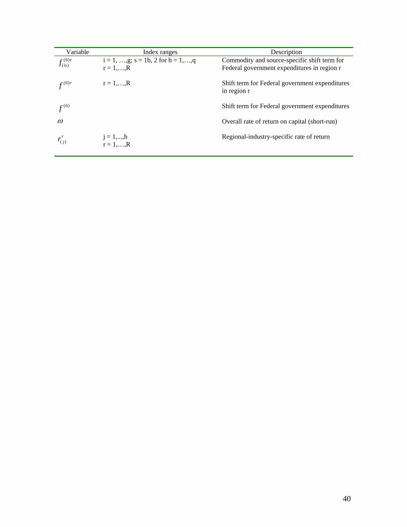
40

Variable Index ranges Description r

isf )6()( i = 1, …,g; s = 1b, 2 for b = 1,…,q

r = 1,…,R Commodity and source-specific shift term for Federal government expenditures in region r

rf )6( r = 1,…,R Shift term for Federal government expenditures in region r

)6(f Shift term for Federal government expenditures

ω Overall rate of return on capital (short-run)

rjr )( j = 1,...,h

r = 1,…,R

Regional-industry-specific rate of return

41

Parameters, Coefficients and Sets

Symbol Description ru

i)(

)(σ Parameter: elasticity of substitution between alternative sources of commodity or factor i for user (u) in region r

rj)0(σ Parameter: elasticity of transformation between outputs of different commodities in industry j in region r

rjsg

)1(),1( +α Parameter: returns to scale to individual primary factors in industry j in region r

ri)(β Parameter: marginal budget shares in linear expenditure system for commodity i in

region r

ri)(γ Parameter: subsistence parameter in linear expenditure system for commodity i in region

r

rj )(ε Parameter: sensitivity of capital growth to rates of return of industry j in region r

ris)(η Parameter: foreign elasticity of demand for commodity i from region r

ru

is)()(θ Parameter: scale economies to transportation of commodity (i) produced in region r

shipped to user (u) in region r

rui

)()( •µ Parameter: returns to scale to primary factors (i = g+1 and u = 1j); otherwise, 1)(

)( =•ru

iµ

)),(,,( rusiB Input-output flow: basic value of (is) used by (u) in region r

),(,,,( rusimM

Input-output flow: basic value of domestic good m used as a margin to facilitate the flow of (is) to (u) in region r

)),(,,,( rusiT τ

Input-output flow: collection of tax τ on the sale of (is) to (u) in region r

)),(,,( rusiV Input-output flow: purchasers’ value of good or factor i from source s used by user (u) in region r

),,( rjiY Input-output flow: basic value of output of domestic good i by industry j from region r rjQ )( Coefficient: ratio, gross to net rate of return

G Set: {1,2, …, g}, g is the number of composite goods

G* Set: {1,2, …, g+1}, g+1 is the number of composite goods and primary factors

H Set: {1,2, …, h}, h is the number of industries

U Set: {(3), (4), (5), (6), (k j) for k = 1, 2 and j = 1, …, h}

U* Set: {(3), (k j) for k = 1, 2 and j = 1, …, h}

S Set: {1, 2, …, r+1}, r+1 is the number of regions (including foreign)

S* Set: {1, 2, …,r}, r is the number of domestic regions

T Set: {1, …, t}, t is the number of indirect taxes

Trade Liberalization and Regional Inequality: Do … · 1 Trade Liberalization and Regional...

Documents

Transcript of Trade Liberalization and Regional Inequality: Do … · 1 Trade Liberalization and Regional...