Regional Flow in the Dakota Aquifer: A Study of the Role of Confining Layers

United States Geological SurveyWater-Supply Paper 2237

Regional Flow in the Dakota Aquifer: A Study of the Role of Confining Layers

ByJ. D. Bredehoeft, C. E. Neuzil, and P. C. D. Milly

U.S. GEOLOGICAL SURVEY WATER-SUPPLY PAPER 2237

UNITED STATES DEPARTMENT OF THE INTERIOR JAMES G. WATT, Secretary

GEOLOGICAL SURVEY Dallas L. Peck, Director

UNITED STATES GOVERNMENT PRINTING OFFICE 1983

For sale by Distribution Branch Text Products Section U.S. Geological Survey 604 South Pickett Street Alexandria, Virginia 22304

Library of Congress Cataloging in Publication Data

Bredehoeft, J. D. (John D.) Regional flow in the Dakota aquifer. (Geological Survey water-supply paper ; 2237) Bibliography: p.Supt. of Docs, no.: I 19.13:22371. Groundwater flow Great Plains. 2. Dakota Aquifer. I.

Neuzil, C. E. II. Milly, P. C. D. III. Title. IV. Series. GB1197.7.B73 1983 553.7'9'09783 83-600246

CONTENTSAbstract 1Introduction 1Geology of the ground-water system 3

Hydraulic conductivity of the Dakota aquifer 8 Simulation of region flow 11

Model analysis 13Model of Cretaceous shale confining layer 17Simulation parameters 20Total flow 21

Cretaceous shale confining layer: In situ and laboratory tests 21Pumping test at Wall, South Dakota 21Slug tests in the Pierre Shale 25Laboratory pulse tests 25Laboratory consolidation tests 27

Discussion of shale hydraulic properties 28Hydraulic conductivity 28Specific storage 29

Transport of sulfate in the ground water 30Distribution of sulfate 31Simulation of sulfate transport 31Sulfate transport in the Inyan Kara Group sandstones 34Sulfate transport in the Dakota-Newcastle Sandstone 34The role of geological membranes in the transport of sulfate 38

Chloride in the ground water 42 Discussion 42

Simplifying assumptions 42 Conclusions 43 Acknowledgments 43 References 44

FIGURES

1. Aquifer system in South Dakota 42. Isolith map of the Inyan Kara Group sandstones 63. Isolith map of the Dakota-Newcastle Sandstone 74. Minor aquifer system above the Dakota Sandstone in South Dakota 105. Graph showing specific capacity versus transmissivity for a flowing well 116. Maps showing distribution of most reliable well hydraulic conductivity data

and third-degree polynomial trend surfaces computed from subsets of the data 12

7. Diagrammatic cross section showing the simplest conceptual model used to analyze the Dakota aquifer 13

8. Sketch depicting the arrangement of finite-difference grids used for the three-aquifer model of the Dakota system 14

9. Map showing virgin potentiometric surface, relative to land surface, for the Dakota aquifer 15

10. Map showing computed virgin potentiometric surface, relative to land sur­ face, for the Dakota aquifer (assumed hydraulic conductivity for the com­ bined Cretaceous shale confining layer of 5 x 10~ 9 ft/sec) 16

11. Map showing computed virgin potentiometric surface, relative to land sur­ face, for the Dakota aquifer (assumed hydraulic conductivity for the com­ bined Cretaceous shale confining layer of 5 x 10~ n ft/sec) 17

III

12. Maps showing virgin potentiometric surface, relative to sea level, for the Dakota aquifer 18

13. Graph showing well discharge and number of wells in the Dakota aquifer 2114. Maps showing potentiometric surface in the Dakota aquifer in 1915 2215. Map showing computed potentiometric surface in the Dakota aquifer for

1908 2416. Sketch showing computed virgin, or steady flow, through the aquifer system

in South Dakota 2517. Map showing computed steady-state leakage through Cretaceous shale con­

fining layer 2618. Plot of drawdown data from pumping test at Wall, South Dakota 2719. Map showing locations of test hole sites 2720. Schematic diagram of slug test setup 2721. Plot of pressure-decay data for a modified slug test in the Pierre Shale 2822. Section showing hydraulic conductivity of the Pierre Shale calculated from

modified slug tests 2823. Summary plot of hydraulic conductivity data for the Cretaceous shale con­

fining layer 3024. Summary plot of specific storage data for the Cretaceous shale confining

layer 3125. Map showing sulfate concentrations in Dakota-Newcastle ground water 3226. Map showing sulfate concentrations in Inyan Kara ground water 3327. Map showing areal distribution of gypsum and anhydrite 3528. Map showing calculated sulfate concentrations for Inyan Kara ground water 3629. Map showing calculated sulfate concentrations for the Dakota-Newcastle

ground water 3730. Graph of net filtration ratio, F, as a function of shale thickness, b 3931. Map showing calculated sulfate concentrations for the Dakota-Newcastle

ground water 4032. Map showing chloride concentrations in Dakota-Newcastle ground water 41

TABLES

1. Summary of hydraulic conductivity estimates for the Dakota Sandstone 92. Summary of Niven's (1967) outcrop data 93. "Best-fit" parameters used in various model analyses 204. Summary of pulse test results for the Pierre Shale 295. Summary of consolidation test results for the Pierre Shale 29

IV

REGIONAL FLOW IN THE DAKOTA AQUIFER: A STUDY OF THE ROLE OF CONFINING LAYERSBy J. D. Bredehoeft, C. E. Neuzil, and P. C. D. Milly

Abstract

The Dakota Sandstone in South Dakota is one of the classic artesian aquifers; it was first studied by N. H. Darton at the turn of the century. Since then, hydrogeologists have debated the source of the large quantities of water which have been discharged by artesian flow from the Dakota. Among suggestions for the source of this water are (1) re­ charge of the aquifer at outcrops in the Black Hills, (2) com­ paction and compressive storage within the aquifer, (3) leak­ age through confining layers, and (4) upward flow from the underlying Madison Group limestones.

A series of increasingly refined models of the aquifer system in South Dakota have been developed and used for numerical simulations of the ground-water flow. The simula­ tions have provided estimates of leakage through the confining layers. The results indicate that, before develop­ ment, most of the flow into and out of the Dakota Sandstone occurred as leakage through confining layers and, since development, most of the water released from storage has come from the confining layers.

In situ and laboratory hydraulic conductivity measure­ ments have been made for the Cretaceous shale confining layer which overlies the Dakota. These data indicate hydrau­ lic conductivities which are one to three orders of magnitude lower than the conductivities indicated by the numerical analyses; this suggests that the leakage through the confining layer is largely through fractures. The fractures apparently did not influence the laboratory and in situ measurements.

To test the conception of flow in the aquifer-confining layer system derived from our analyses, the transport of sulfate in the system was simulated. Simulations using a numerical ground-water transport model were reasonably successful in explaining the present distribution of sulfate in the system. This result increases confidence in the flow sys­ tem implied by the flow simulations in which leakage through confining layers is dominant.

INTRODUCTION

The Dakota aquifer in South Dakota is one of the classic artesian aquifers. Many modern ideas concerning artesian aquifers stem from N. H. Darton's investi­

gation of the Dakota aquifer in the 1890's and early 1900's. This paper is based to a large extent upon Darton's data and is a tribute to Darton's ability as a hydrologist.

It is clear from examining Darton's work that he understood most aspects of the ground-water hydrology of the Dakota aquifer. In 1896, he published a prelimi­ nary report which described the system (Darton, 1896). He and workers under his direction then proceeded sys­ tematically to map the area of principal ground-water development along the James River in eastern South Dakota; much of the actual mapping was done by J. E. Todd under Darton's direction. A series of Geologic Folios were published which covered the ground-water geology of the James River lowland from Nebraska to North Dakota. These folios, designed to display the ground-water geology of the area, are classic examples of hydrogeologic mapping.

While Todd mapped the area of major develop­ ment, Darton mapped the entire Black Hills in four quadrangles. The Black Hills area included the Dakota outcrop, a source of recharge for the Dakota aquifer in South Dakota. Darton (1909) summarized his Dakota investigations in U.S. Geological Survey Water-Supply Paper 227. He pointed out that the potentiometric head within the Dakota system is controlled by the elevation of the sandstone outcrops in the Black Hills and set forth his ideas concerning the mechanics of the system in the following remarks (Darton, 1909, p. 60):

"The evidence of this pressure, as found in many wells in eastern South Dakota, is conclusive that the water flows underground for many hundreds of miles. Such pressures can be explained only by the hydrostatic influence of a column of water extending to a high altitude on the west. If it were not for the outflow of the water to the east and south the initial head which the waters derived from the high lands of the intake zone would continue under the entire region, but owing to this leakage the head is not maintained, and there is a gradual diminution toward the east known as 'hydraulic grade/ a slope sustained by the friction of the water in its passage through the strata."

1

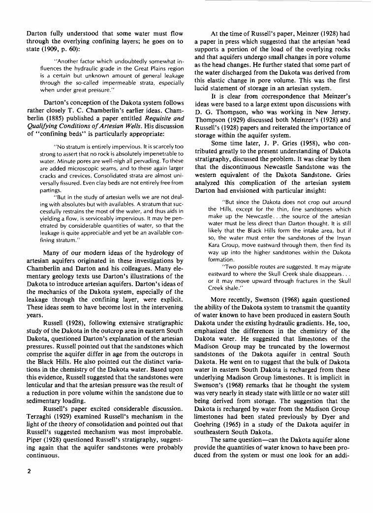
Darton fully understood that some water must flow through the overlying confining layers; he goes on to state (1909, p. 60):

"Another factor which undoubtedly somewhat in­ fluences the hydraulic grade in the Great Plains region is a certain but unknown amount of general leakage through the so-called impermeable strata, especially when under great pressure."

Darton's conception of the Dakota system follows rather closely T. C. Chamberlin's earlier ideas. Cham- berlin (1885) published a paper entitled Requisite and Qualifying Conditions of Artesian Wells. His discussion of "confining beds" is particularly appropriate:

"No stratum is entirely impervious. It is scarcely too strong to assert that no rock is absolutely impenetrable to water. Minute pores are well-nigh all pervading. To these are added microscopic seams, and to these again larger cracks and crevices. Consolidated strata are almost uni­ versally fissured. Even clay beds are not entirely free from partings.

"But in the study of artesian wells we are not deal­ ing with absolutes but with availables. A stratum that suc­ cessfully restrains the most of the water, and thus aids in yielding a flow, is serviceably impervious. It may be pen­ etrated by considerable quantities of water, so that the leakage is quite appreciable and yet be an available con­ fining stratum."

Many of our modern ideas of the hydrology of artesian aquifers originated in these investigations by Chamberlin and Darton and his colleagues. Many ele­ mentary geology texts use Darton's illustrations of the Dakota to introduce artesian aquifers. Darton's ideas of the mechanics of the Dakota system, especially of the leakage through the confining layer, were explicit. These ideas seem to have become lost in the intervening years.

Russell (1928), following extensive stratigraphic study of the Dakota in the outcrop area in eastern South Dakota, questioned Darton's explanation of the artesian pressures. Russell pointed out that the sandstones which comprise the aquifer differ in age from the outcrops in the Black Hills. He also pointed out the distinct varia­ tions in the chemistry of the Dakota water. Based upon this evidence, Russell suggested that the sandstones were lenticular and that the artesian pressure was the result of a reduction in pore volume within the sandstone due to sedimentary loading.

Russell's paper excited considerable discussion. Terzaghi (1929) examined Russell's mechanism in the light of the theory of consolidation and pointed out that Russell's suggested mechanism was most improbable. Piper (1928) questioned Russell's stratigraphy, suggest­ ing again that the aquifer sandstones were probably continuous.

At the time of Russell's paper, Meinzer (1928) had a paper in press which suggested that the artesian head supports a portion of the load of the overlying rocks and that aquifers undergo small changes in pore volume as the head changes. He further stated that some part of the water discharged from the Dakota was derived from this elastic change in pore volume. This was the first lucid statement of storage in an artesian system.

It is clear from correspondence that Meinzer's ideas were based to a large extent upon discussions with D. G. Thompson, who was working in New Jersey. Thompson (1929) discussed both Meinzer's (1928) and Russell's (1928) papers and reiterated the importance of storage within the aquifer system.

Some time later, J. P. Gries (1958), who con­ tributed greatly to the present understanding of Dakota stratigraphy, discussed the problem. It was clear by then that the discontinuous Newcastle Sandstone was the western equivalent of the Dakota Sandstone. Gries analyzed this complication of the artesian system Darton had envisioned with particular insight:

"But since the Dakota does not crop out around the Hills, except for the thin, fine sandstones which make up the Newcastle. . .the source of the artesian water must be less direct than Darton thought. It is still likely that the Black Hills form the intake area, but if so, the water must enter the sandstones of the Inyan Kara Group, move eastward through them, then find its way up into the higher sandstones within the Dakota formation.

"Two possible routes are suggested. It may migrate eastward to where the Skull Creek shale disappears. .. or it may move upward through fractures in the Skull Creek shale."

More recently, Swenson (1968) again questioned the ability of the Dakota system to transmit the quantity of water known to have been produced in eastern South Dakota under the existing hydraulic gradients. He, too, emphasized the differences in the chemistry of the Dakota water. He suggested that limestones of the Madison Group may be truncated by the lowermost sandstones of the Dakota aquifer in central South Dakota. He went on to suggest that the bulk of Dakota water in eastern South Dakota is recharged from these underlying Madison Group limestones. It is implicit in Swenson's (1968) remarks that he thought the system was very nearly in steady state with little or no water still being derived from storage. The suggestion that the Dakota is recharged by water from the Madison Group limestones had been stated previously by Dyer and Goehring (1965) in a study of the Dakota aquifer in southeastern South Dakota.

The same question can the Dakota aquifer alone provide the quantities of water known to have been pro­ duced from the system or must one look for an addi-

tional source? is implied in each of the discussions following Darton. This report describes our analysis, using numerical simulations, of the hydrodynamics and geochemistry of the Dakota aquifer and suggests answers to the question posed above. Recognizing that low-permeability confining layers and high-permeability aquifers are interacting parts of a single system, this in­ vestigation was directed toward understanding the aquifer system as a whole. The flow was first simulated using a very simplified model of the system, which con­ sisted of a single aquifer, the Dakota, confined by one leaky confining layer, the Cretaceous shales. The original model was then refined by adding the Madison aquifer and confining layer and then by subdividing the Dakota into two aquifers in western South Dakota, the Inyan Kara and Newcastle, with the appropriate inter­ vening confining layer.

Even though the Dakota aquifer has been studied for almost 90 years, relatively little published data con­ cerning its hydraulic conductivity exists. Niven (1967) measured the hydraulic conductivity of approximately 300 samples taken from the outcrops of the Inyan Kara and Newscastle sandstones in the Black Hills. A test was run on a well at Box Elder, South Dakota, near the out­ crop area of the sands on the east flank of the Black Hills (Miller and Rahn, 1974), and another was con­ ducted at Wall, South Dakota (Gries and others, 1976). These data comprise the published hydraulic conductivi­ ty information for the Dakota aquifer in South Dakota.

During the course of this study, Martin Sather, a water-well drilling contractor in Presho, South Dakota, made available the records of the Norbeck and Hollis Drilling Company. This firm was perhaps the largest drilling company in South Dakota in the early 1900's, operating some 27 rigs at one time. Only the drilling reports are available; however, it is possible to estimate the hydraulic conductivity of the aquifer through care­ ful use of these data. This was done for approximately 500 wells drilled in the years 1904 through 1908.

Darton (1909) published a regional potentiometric surface for the Dakota aquifer using the earliest available drilling reports. By the time his report was published, more than 1,000 wells had penetrated the Dakota, most of which flowed. Rothrock had Robinson (1936), Erickson (1954, 1955), Barkley (1953), and Schoon (1971) document the historic change in the potentiometric surface, and Davis and others (1961) describe its effect on wells in South Dakota. Because of the aquifer's importance to South Dakota's water sup­ ply, relatively complete records of rates and locations of water withdrawal from the Dakota Sandstone were made, beginning shortly after the start of development. These records are available in the biennial and annual reports of the South Dakota State Engineer. Together, these data document the withdrawal of water from the

aquifer and the resulting change in the potentiometric surface.

GEOLOGY OF THE GROUND-WATER SYSTEM

Present day South Dakota was a site of sedimen­ tary deposition from Paleozoic to Tertiary time. Except for Tertiary deposits which have largely been removed by erosion, most of the sedimentary formations are still present in the western part of the State. In the eastern part of South Dakota, much of the younger sedimentary cover has been removed. Structurally, there is a north- south-trending shallow trough with its axis west of the center of the State. Two structural highs exist: the Sioux Ridge, a gentle high of Precambrian quartzite, near the eastern edge of the State and the Black Hills, a dome of crystalline Precambrian rocks with younger sedimentary strata dipping outward on its flanks, along the western edge of the State.

Elevations are highest in the Black Hills area and diminish more or less uniformly to the east. This trend is broken by the deeply eroded valley of the Missouri River, the so-called Missouri Trench. Outcrops of the major aquifers are generally at an altitude of 3,000 to 4,000 ft around the Black Hills. Outcrops of the Dakota Sandstone in the eastern part of the State are at an altitude of approximately 1,000 ft. In roughly the western half of the State, west of the Missouri River, the terrain is quite old, with several rivers which flow ap­ proximately from west to east draining to the Missouri. Pleistocene till dissected by a postglacial drainage system blankets most of the area east of the Missouri River.

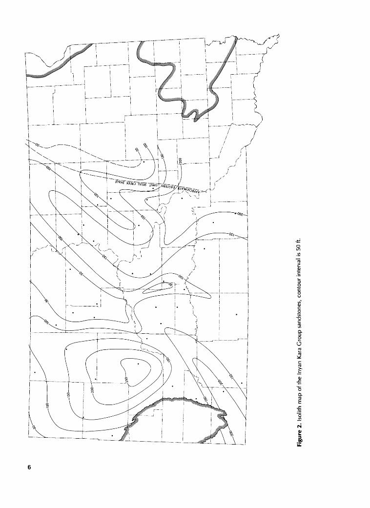
The ground-water system is dominated by three major aquifers (Darton, 1909; Gries, 1958; Swenson, 1968; Schoon, 1971). The areas of aquifer outcrop are shown in figure I A, and a schematic cross section of the aquifers and their confining layers is presented in figure IB. The lowest aquifer, primarily Mississippian carbonate rocks collectively called the Madison Group, terminates in the subsurface beneath the Inyan Kara Group sand­ stones (Swenson, 1968; Schoon, 1971). The Inyan Kara Group and the Newcastle Sandstone, both distinct aquifers in the western portion of the State, merge to form the Dakota Sandstone in the eastern part of the State (Gries, 1958; Schoon, 1971). All three aquifers, the Madison, the Inyan Kara, and the Dakota- Newcastle, crop out on the flanks of the Black Hills, although the Newcastle Sandstone may be discon­ tinuous eastward (Gries, 1958; Schoon, 1971). The Dakota crops out in the extreme eastern part of South Dakota.

Although it remained for Gries (1954, 1958) and others to sort out the Dakota and Inyan Kara stratig-

r . - - -r

! L<

' i

V i

1 -

y !

i '^

" '

1"

1 ,

^

;

i --

; !

- i

i /«

f

i "I

'--.

r^

i

: i

! , -

.-'»

r s

i i

, ^

"""r

o i

'M

^ i

i --

^

) °

i i

"T

L^k.

"" ~

' - /

\ (

S

1 '

r%B

,--i-

i '

-7

i i

1 a\\

/ i

! ~~

v->

i i_

_

1 T

l 7

i !

\ /

[ '

X

('._

._

._

._

-4

1

\_--j

\ \

I ;

1 ^-

\

A^ -

\

\ \

-^^\

\ i

r ' '

%

i--- -- V

.-.-T

--

1--,

\l

! i

L..

-Ni

! '

-- -

- -4

l

i '

1 ;

l_ - H

1

' 1

1 1 !l|

' -

] "I

' '

i i

'' 1

! i

; ^

i "s

ioiu

xi

RID

GE

100

MIL

ES

-<

// >

-.K

.

100

KIL

OM

ET

ER

S

Fig

ure

1.

Aq

uife

r sy

stem

in

Sou

th D

akot

a. A

, O

utcr

ops

of

the

maj

or a

quife

rs:

Dak

ota-

New

cast

le S

ands

tone

(A

); In

yan

Kar

a G

roup

san

dsto

nes

(B);

Mad

ison

Gro

up

limest

ones

(C).

The

Dak

ota

San

dsto

ne s

how

n in

the

eas

tern

pa

rt o

f th

e st

ate

is ge

nera

lly o

bscu

red

by P

leis

toce

ne d

epos

its.

B,

Sch

emat

ic e

ast-

wes

t cr

oss

sect

ion.

V

ert

ical

scal

e is

gre

atly

exa

gger

ated

.

BLACK HILLS SOUTH ) DAKOTA

W

1

PLEISTOCENE DEPOSITS L

CRETACEOUS SHALE CONFINING LAYER^RTZITE

B

Figure 1. Continued.

raphy, Barton's (1901, 1909) conception of the gross ground-water flow in the system was much the same as is understood today. The aquifers are partly recharged at high elevations around the Black Hills and conduct water toward the east. In eastern South Dakota, out­ crops permit discharge. Darton (1909, p. 60) believed recharge and discharge also occur by leakage through confining layers, as pointed out above.

Separating the major aquifers are confining layers of low-permeability rock. The confining layer overlying the Madison, in this report called the "Madison confin­ ing layer," encompasses the section from the top of the Mississippian carbonate rocks to the base of the Inyan Kara Group sandstones and includes some aquifers of minor importance. Swenson (1968) suggested that the Madison subcrops directly beneath parts of the Inyan Kara. The Madison confining layer thins eastward, but significantly different potentiometric heads in the Madi­ son and Inyan Kara indicate that it completely separates them.

The Skull Creek Shale separates the Inyan Kara Group from the overlying Dakota-Newcastle Sandstone. It thins eastward and eventually pinches out, which allows the Inyan Kara and Newcastle sands to merge, forming the Dakota Sandstone of eastern South Dakota (Gries, 1958; Schoon, 1971).

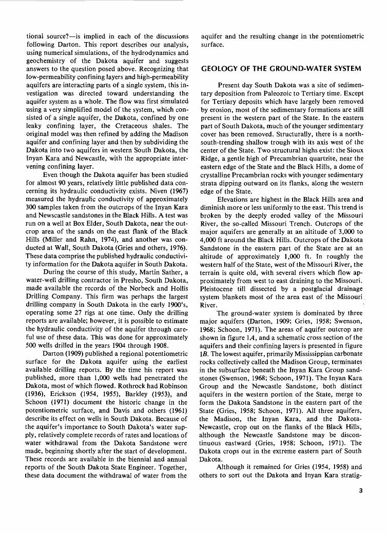
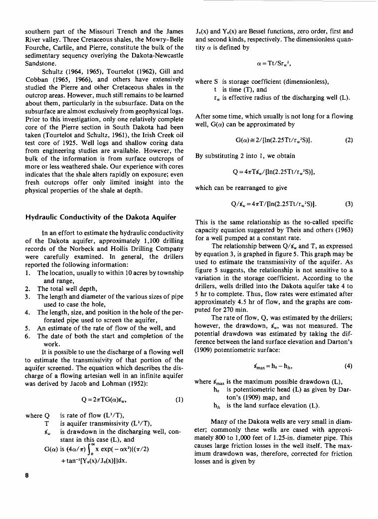
To carry out our investigation, it was necessary to estimate the transmissivity and its areal variation in each aquifer. The thickness of the aquifers was, therefore, important, and isolith maps of the units were prepared, largely from a regional selection of electric logs. The

isolith map of the Inyan Kara Group is shown in figure 2. Figure 3 is the isolith map of the Dakota-Newcastle Sandstone.

As noted above, Gries (1958) indicates that the Newcastle Sandstone is quite thin and may be dis­ continuous in western South Dakota. However, subsur­ face correlations suggest that the sandstones tend to be continuous; at least within certain stratigraphic inter­ vals, sand bodies tend to be present. The density of con­ trol is not sufficient to indicate whether individual sand bodies are isolated from one another. However, these intervals are zones of higher permeability which contain sufficiently large percentages of sand to make it reason­ able to expect each to be hydraulically continuous.

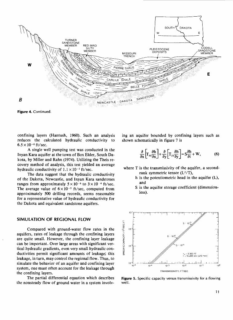
The confining layer overlying the Dakota, which we call the "Cretaceous shale confining layer," includes the entire sequence above the Dakota-Newcastle Sand­ stone. Sedimentary rocks from this dominantly shale se­ quence crop out over much of South Dakota. Although predominanted by shales, the Cretaceous shale confin­ ing layer contains several minor aquifers, most impor­ tant of which are the Niobrara Formation (predominant­ ly chalk) and the Greenhorn Limestone.

The outcrops of the Niobrara and Greenhorn aquifers are shown in figure 4A; the stratigraphy of the Cretaceous shale confining layers is presented schematically figure 4B. Like the Dakota-Newcastle Sandstone, the Niobrara Formation and Greenhorn Limestone aquifers both crop out on the flanks of the Black Hills and again in the extreme eastern part of the State; the Niobrara Formation also crops out in the

Figu

re 2

. Is

olith

map

of t

he I

nyan

Kar

a G

roup

san

dsto

nes,

conto

ur

inte

rval

is

50 f

t.

Figu

re 3

. Is

olith

map

of

the

Dak

ota-

New

cast

le S

ands

tone

, co

ntou

r in

terv

al i

s 50

ft.

southern part of the Missouri Trench and the James River valley. Three Cretaceous shales, the Mo wry-Belle Fourche, Carlile, and Pierre, constitute the bulk of the sedimentary sequency overlying the Dakota-Newcastle Sandstone.

Schultz (1964, 1965), Tourtelot (1962), Gill and Cobban (1965, 1966), and others have extensively studied the Pierre and other Cretaceous shales in the outcrop areas. However, much still remains to be learned about them, particularly in the subsurface. Data on the subsurface are almost exclusively from geophysical logs. Prior to this investigation, only one relatively complete core of the Pierre section in South Dakota had been taken (Tourtelot and Schultz, 1961), the Irish Creek oil test core of 1925. Well logs and shallow coring data from engineering studies are available. However, the bulk of the information is from surface outcrops of more or less weathered shale. Our experience with cores indicates that the shale alters rapidly on exposure; even fresh outcrops offer only limited insight into the physical properties of the shale at depth.

Hydraulic Conductivity of the Dakota Aquifer

In an effort to estimate the hydraulic conductivity of the Dakota aquifer, approximately 1,100 drilling records of the Norbeck and Hollis Drilling Company were carefully examined. In general, the drillers reported the following information:1. The location, usually to within 10 acres by township

and range,2. The total well depth,3. The length and diameter of the various sizes of pipe

used to case the hole,4. The length, size, and position in the hole of the per­

forated pipe used to screen the aquifer,5. An estimate of the rate of flow of the well, and6. The date of both the start and completion of the

work.It is possible to use the discharge of a flowing well

to estimate the transmissivity of that portion of the aquifer screened. The equation which describes the dis­ charge of a flowing artesian well in an infinite aquifer was derived by Jacob and Lohman (1952):

(1)

where Q T

is rate of flow (LVT),is aquifer transmissivity (LVT),

tfw is drawdown in the discharging well, con­ stant in this case (L), and

G(a) is (4a/7r) (°°x exp(-ax2)((7r/2)Jo

+ tan- 1 [Yo(x)/J0(x)])dx.

J0 (x) and Y0 (x) are Bessel functions, zero order, first and and second kinds, respectively. The dimensionless quan­ tity a is defined by

a = Tt/Srw2 ,

where S is storage coefficient (dimensionless), t is time (T), and rw is effective radius of the discharging well (L).

After some time, which usually is not long for a flowing well, G(a) can be approximated by

G(a) = 2/[ln(2.25Tt/rw 2 S)]. (2)

By substituting 2 into 1, we obtain

Q = 47rT*w/[ln(2.25Tt/rw 2 S)],

which can be rearranged to give

w = 47rT/[ln(2.25Tt/rw 2 S)]. (3)

This is the same relationship as the so-called specific capacity equation suggested by Theis and others (1963) for a well pumped at a constant rate.

The relationship between Q/tfw and T, as expressed by equation 3, is graphed in figure 5. This graph may be used to estimate the transmissivity of the aquifer. As figure 5 suggests, the relationship is not sensitive to a variation in the storage coefficient. According to the drillers, wells drilled into the Dakota aquifer take 4 to 5 hr to complete. Thus, flow rates were estimated after approximately 4.5 hr of flow, and the graphs are com­ puted for 270 min.

The rate of flow, Q, was estimated by the drillers; however, the drawdown, tfw , was not measured. The potential drawdown was estimated by taking the dif­ ference between the land surface elevation and Darton's (1909) potentiometric surface:

"max = "o ~ ll/s» VT)

where tfmax is the maximum possible drawdown (L),h0 is potentiometric head (L) as given by Dar­

ton's (1909) map, and h/s is the land surface elevation (L).

Many of the Dakota wells are very small in diam­ eter; commonly these wells are cased with approxi­ mately 800 to 1,000 feet of 1.25-in. diameter pipe. This causes large friction losses in the well itself. The max­ imum drawdown was, therefore, corrected for friction losses and is given by

(5)

where tff/ is the loss in head due to friction losses in the casing (L).

It was not uncommon to find in the drilling data that the computed friction losses were greater than the available head. This probably indicates that the driller did not make a reliable flow estimate. In some cases, error in the estimates of h0 and h/s or in the completion time may have been significant. Such data were dis­ carded. Discarding this portion of the data preferentially removed only errors of overestimated flow; however, these probably represent the majority of errors. Over­ estimates of well yields were probably more common than underestimates.

The drilling data also provided a crude check of Darton's map. Wells should flow only where the aquifer potentiometric surface is above the land surface eleva­ tion. This check indicated that Darton's map is reliable in the areas of development.

The transmissivity was estimated using the rela­ tionship shown in figure 5. Transmissivity estimates were then divided by the interval screened in the well to obtain an estimate of the hydraulic conductivity. The conductivity estimates are summarized by counties in table 1. In Beadle, Brown, and Spink Counties, trans­ missivity estimates were computed for approximately 100 wells in each county. Approximately 500 records were thought to give reasonably reliable results; of these, about 300 were thought to be very good. The dis­ tribution of the most reliable data is shown in figure 6.

Unfortunately, most of the highly reliable data are in a limited area in northeast South Dakota, which pro-

Table 1. Summary of hydraulic conductivity estimates for the Dakota Sandstone

Number of County wells

D^orll A

PlarV

Edmunds ----- FaulkHandKingsbury Marshall and Day Sandborn and Miner Spink -- Stanley and Hughes Sully

112 110

6 5

75 11 41 20 10 88

7 9

Mean hydraulic conductivity (10- 5 ft/sec)

6.7 5.4 3.0 3.0 7.0

11.0 2.1 3.5 3.9

11.0 5.7 2.1

Standard deviation

(10- 5 ft/sec)

6.0 6.2 2.2 1.4 7.1 8.8 2.9 3.5 5.5

11.0 6.4 3.0

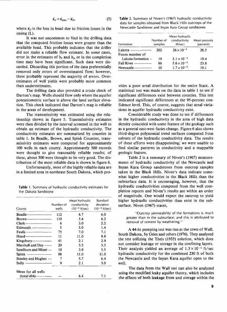
Table 2. Summary of Niven's (1967) hydraulic conductivity data for samples obtained from Black Hills outcrops of the Newcastle Sandstone and Inyan Kara Group sandstones

Mean hydraulicNumber of conductivity Mean porosity

Formation samples (ft/sec) (percent)

T dVritci

Fuson member of Lakota formation -

Fall River

202

19Q£

10

26xlO- 5

3.1xlO~ 5 5.6X10- 51 7 x 10~ 5

-)o e

19.471 8

19.1

Mean for all wells (total 494) - 6.4 7.1

vides a poor areal distribution for the entire State. A statistical test was made on the data in table 1 to see if significant differences exist between counties. This test indicated significant differences at the 95-percent con­ fidence level. This, of course, suggests that areal varia­ tions in aquifer hydraulic conductivity exist.

Considerable study was done to see if differences in the hydraulic conductivity in the area of high data density coincided with some feature of the geology such as a general east-west facies change. Figure 6 also shows third-degree polynomial trend surfaces computed from subsets of the hydraulic conductivity data. The results of these efforts were disappointing; we were unable to find similar patterns in conductivity and a mappable geologic feature.

Table 2 is a summary of Niven's (1967) measure­ ments of hydraulic conductivity of the Newcastle and Inyan Kara Group sandstones from outcrop samples taken in the Black Hills. Niven's data indicate some­ what higher conductivities in the Black Hills than the subsurface data. It is encouraging, however, that the hydraulic conductivities computed from the well com­ pletion reports and Niven's results are within an order of magnitude. One would expect the outcrop to yield higher hydraulic conductivities than exist in the sub­ surface. Niven (1967) states,

"Outcrop permeability of the formations is much greater than in the subsurface, and this is attributed to removal of cement by weathering."

A 44-hr pumping test was run at the town of Wall, South Dakota, by Gries and others (1976). They analyzed the test utilizing the Theis (1935) solution, which does not consider leakage or storage in the confining layers. Their analysis yielded an average of 1.5xlO~ 5 ft/sec hydraulic conductivity for the combined 230 ft of both the Newcastle and the Inyan Kara aquifer open to the well.

The data from the Wall test can also be analyzed using the modified leaky aquifer theory, which includes the effects of both leakage from and storage within the

I

'\ \ ,_

J

c_

; ;,

1 1 i -i-

. -

-

i \- 1 i 1 i i

0 I

0

100

MIL

ES

j

100

KIL

OM

ET

ER

S

Figu

re 4

. M

inor

aquife

r sy

stem

abo

ve t

he

Dak

ota

San

dsto

ne i

n S

outh

D

akot

a. A

, O

utcr

ops

of

the

Nio

brar

a F

orm

atio

n (A

) an

d th

e G

reen

horn

Li

mes

tone

(B

). E

ast

of

the

Mis

souri

tren

ch t

he b

edro

ck i

s ge

nera

lly o

bscu

red

by P

leis

toce

ne d

epos

its.

B,

Sch

emat

ic e

ast-

wes

t cr

oss-

sect

ion

of

the

"Cre

tace

ous

shal

e co

nfin

ing

la

yer.

" V

ert

ica

l sc

ale

is g

reat

ly e

xagg

erat

ed.

TURNER SANDSTONE

MEMBER RED BIRDSILTY

MEMBER

w

B

Figure 4. Continued.

NEWCASTLE'DAKOTA

confining layers (Hantush, 1960). Such an analysis reduces the calculated hydraulic conductivity to 6.5 x 10~ 6 ft/sec.

A single well pumping test was conducted in the Inyan Kara aquifer at the town of Box Elder, South Da­ kota, by Miller and Rahn (1974). Utilizing the Theis re­ covery method of analysis, this test yielded an average hydraulic conductivity of 1.1 x 10~ 5 ft/sec.

The data suggest that the hydraulic conductivity of the Dakota, Newcastle, and Inyan Kara sandstones ranges from approximately 5xlO- 6 to3xlO~4 ft/sec. The average value of 6xlO~ 5 ft/sec, computed from approximately 500 drilling records, seems reasonable for a representative value of hydraulic conductivity for the Dakota and equivalent sandstone aquifers.

SIMULATION OF REGIONAL FLOW

Compared with ground-water flow rates in the aquifers, rates of leakage through the confining layers are quite small. However, the confining layer leakage can be important. Over large areas with significant ver­ tical hydraulic gradients, even very small hydraulic con­ ductivities permit significant amounts of leakage; this leakage, in turn, may control the regional flow. Thus, to simulate the behavior of an aquifer and confining layer system, one must often account for the leakage through the confining layers.

The partial differential equation which describes the nonsteady flow of ground water in a system involv­

ing an aquifer bounded by confining layers such as shown schematically in figure 7 is

ah e [ ah] ^ L1^ J = + w'

where T is the transmissivity of the aquifer, a second- rank symmetric tensor (LVT),

h is the potentiometric head in the aquifer (L), and

S is the aquifer storage coefficient (dimension- less).

10-4 10-3 10-2

TRANSMISSIVITY, FT/SEC

10°

Figure 5. Specific capacity versus transmissivity for a flowing well.

11

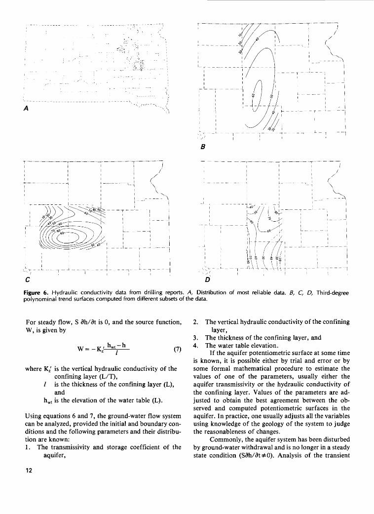
Figure 6. Hydraulic conductivity data from drilling reports. A, Distribution of most reliable data. B, C, D, Third-degree polynominal trend surfaces computed from different subsets of the data.

For steady flow, S dh/dt is 0, and the source function, W, is given by

W=-KZ' hwt ~ h(7)

where Kz' is the vertical hydraulic conductivity of theconfining layer (L/T),

/ is the thickness of the confining layer (L),and

hwt is the elevation of the water table (L).

Using equations 6 and 7, the ground-water flow system can be analyzed, provided the initial and boundary con­ ditions and the following parameters and their distribu­ tion are known:1. The transmissivity and storage coefficient of the

aquifer,

2. The vertical hydraulic conductivity of the confining layer,

3. The thickness of the confining layer, and4. The water table elevation.

If the aquifer potentiometric surface at some time is known, it is possible either by trial and error or by some formal mathematical procedure to estimate the values of one of the parameters, usually either the aquifer transmissivity or the hydraulic conductivity of the confining layer. Values of the parameters are ad­ justed to obtain the best agreement between the ob­ served and computed potentiometric surfaces in the aquifer. In practice, one usually adjusts all the variables using knowledge of the geology of the system to judge the reasonableness of changes.

Commonly, the aquifer system has been disturbed by ground-water withdrawal and is no longer in a steady state condition (Sdh/dt =£()). Analysis of the transient

12

state provides estimates of the storage properties of the aquifers and confining layers.

Transient vertical leakage in the confining layers is governed by

S' ahK; at (8)

where Ss'is the specific storage (L" 1) and z is vertical dis­ tance in the confining layer.

The gradient of potentiometric head in the confin­ ing layer at the boundary with the aquifer, ah(z,t)/az at z = 0, is determined by equation 8 and its initial and boundary conditions. The boundary conditions are the potentiometric heads in the adjoining aquifers. The source function, W, is then given by

W=-K , dh(z,t)az z = 0 (9)

Methods can be introduced to calculate the tran­ sient source function using equations 8 and 9 and thus account for the effect of storage in the confining layer. In the case of the Dakota, storage within the confining layers is an important part of the analysis, as will be shown below.

Model Analysis

Four conceptual models of the Dakota aquifer system have been used as bases for numerical simula­ tions of the flow. These evolved from a simple model in which the Inyan Kara Group and the Dakota-Newcastle Sandstone were considered a single aquifer underlain by impermeable rocks and overlain by a single homo­ geneous confining layer of varying thickness (the con­ ceptual model shown in fig. 7). The second model in­ cluded a second aquifer below the Dakota representing

Fluid movement 1 \\V > \ V v ' '" Confined aquifer

Confining beds

Figure 7. Diagrammatic cross section of the simplest concep­ tual model used to analyze the Dakota aquifer.

the Madison Group aquifer. The next refinement, which resulted in the third model, was a third aquifer in the western part of South Dakota where the Newcastle and Inyan Kara sandstones are distinct. In terms of the Cretaceous confining layer, a further refinement was in­ troduced by subdividing the confining layer in a fourth model which included only one major aquifer, the Dakota-Newcastle Sandstone. The confining layer was subdivided, as shown in figure 4B, into the Pierre Shale; the Niobrara Formation, an aquifer; the Carlile Shale; the Greenhorn Limestone, also an aquifer; and the Mowry-Belle Fourche Shale.

In all the analyses, the computed potentiometric surface for the aquifers was found to be quite sensitive to Kz'< the confining layer vertical hydraulic conductivi­ ty, indicating that the confining layers and the aquifers interacted significantly and that leakage through the confining layers is an important aspect of system behavior. In transient simulations, it was found that, if leakage from storage in the confining layers was not in­ cluded, drawdowns were much too large.

The ground-water equations were solved using the quasi-three-dimensional finite-difference model by Trescott (1975), which was derived from that of Brede- hoeft and Finder (1970). Each aquifer is represented by a single layer of block-centered nodes. The variable aquifer thickness is accounted for by specifying the value of transmissivity for each block. For multiple aquifers, the model is actually a sequence of two-dimen­ sional aquifer layers coupled to simulate flow through the intervening confining beds.

The grids used for numerical simulations in all of the models were oriented approximately along the car­ dinal directions with equal grid spacing in the north- south and east-west directions. The grid for the first three models was 50 blocks east-west by 36 blocks north-south and covered an area somewhat larger than South Dakota; the blocks were approximately 8.3 mi on a side. The grid for the fourth, or Cretaceous confining layer model, was twice as coarse and contained 25 by 18 nodes.

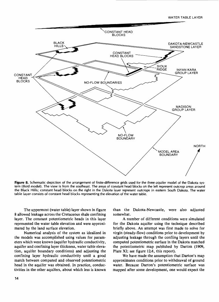
Figure 8 shows the arrangement of the finite- difference grids for the third, or three-aquifer, model. Constant head boundaries were placed at areas of aquifer outcrop; the potentiometric heads assigned represented the elevation at which recharge or discharge occurred. The north and south model boundaries, which are approximately parallel to the general flow from west to east, were treated as impermeable or no- flow boundaries. The eastern no-flow boundary of the Madison layer represented the truncation of the Madi­ son rocks beneath the Madison confining layer. That of the Inyan Kara layer was placed where the Inyan Kara and Dakota merge; east of this boundary, the Dakota layer included both.

13

WATER TABLE LAYER

^CONSTANT HEAD BLOCKS

BLACK HILLS

CONSTANTHEAD

BLOCKS

CONSTANT HEAD BLOCKS

NO-FLOW BOUNDARIES

DAKOTA-NEWCASTLE SANDSTONE LAYER

INYAN KARA GROUP LAYER

MADISON GROUP LAYER

NORTH

MODEL AREA BOUNDARY

Figure 8. Schematic depiction of the arrangement of finite-difference grids used for the three-aquifer model of the Dakota sys­ tem (third model). The view is from the southeast. The areas of constant head blocks on the left represent outcrop areas around the Black Hills; constant head blocks on the right in the Dakota layer represent outcrops in eastern South Dakota. The water table layer consists of constant head blocks representing the elevation of the water table.

The uppermost (water table) layer shown in figure 8 allowed leakage across the Cretaceous shale confining layer. The constant potentiometric heads in this layer represented the water table elevation and were approxi­ mated by the land surface elevation.

Numerical analysis of the system as idealized in the models was accomplished using values for param­ eters which were known (aquifer hydraulic conductivity, aquifer and confining layer thickness, water table eleva­ tion, aquifer boundary conditions) and adjusting the confining layer hydraulic conductivity until a good match between computed and observed potentiometric head in the aquifer was obtained. In practice, conduc­ tivities in the other aquifers, about which less is known

than the Dakota-Newcastle, were also adjusted somewhat.

A number of different conditions were simulated for the Dakota aquifer using the technique described briefly above. An attempt was first made to solve for virgin (steady-flow) conditions prior to development by adjusting leakage through the confiing layers until the computed potentiometric surface in the Dakota matched the potentiometric map published by Darton (1909, Plate XI; see figure 12A, this report).

We have made the assumption that Darton's map approximates conditions prior to withdrawal of ground water. Because Darton's potentiometric surface was mapped after some development, one would expect the

14

virgin surface to be somewhat higher than the surface mapped by Darton and shown in figure 12^4. However, comparison of Barton's map data and the records of the State Engineer reveal that Darton used data from some of the earliest wells drilled. It seems reasonable to assume that Barton's potentiometric surface closely ap­ proximates predevelopment conditions.

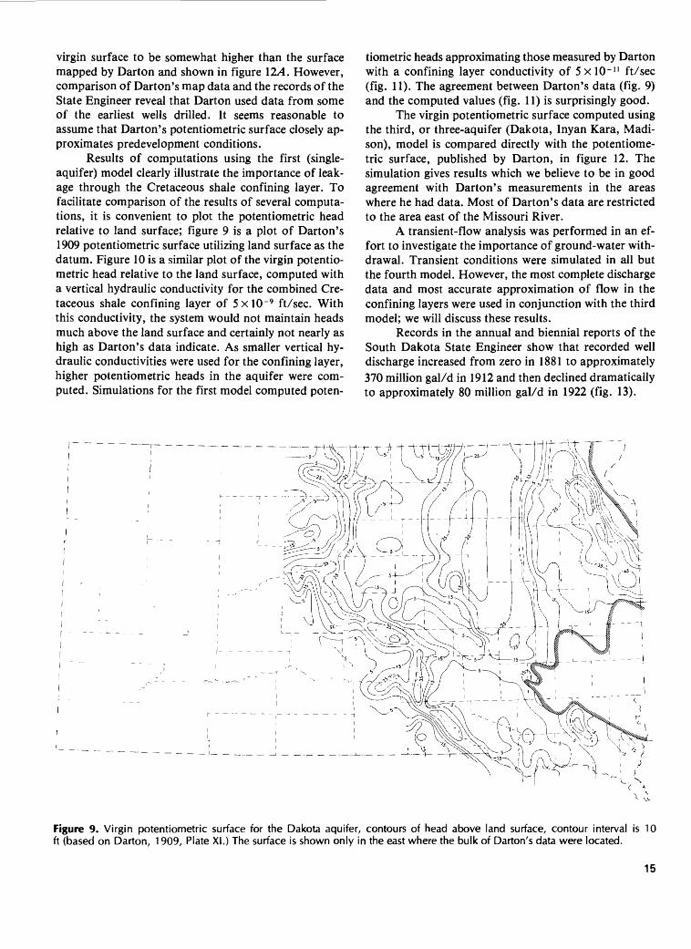
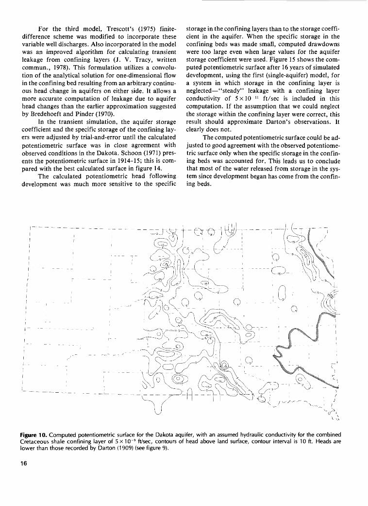
Results of computations using the first (single- aquifer) model clearly illustrate the importance of leak­ age through the Cretaceous shale confining layer. To facilitate comparison of the results of several computa­ tions, it is convenient to plot the potentiometric head relative to land surface; figure 9 is a plot of Barton's 1909 potentiometric surface utilizing land surface as the datum. Figure 10 is a similar plot of the virgin potentio­ metric head relative to the land surface, computed with a vertical hydraulic conductivity for the combined Cre­ taceous shale confining layer of 5 x 10~ 9 ft/sec. With this conductivity, the system would not maintain heads much above the land surface and certainly not nearly as high as Barton's data indicate. As smaller vertical hy­ draulic conductivities were used for the confining layer, higher potentiometric heads in the aquifer were com­ puted. Simulations for the first model computed poten­

tiometric heads approximating those measured by Barton with a confining layer conductivity of 5xlO~ n ft/sec (fig. 11). The agreement between Barton's data (fig. 9) and the computed values (fig. 11) is surprisingly good.

The virgin potentiometric surface computed using the third, or three-aquifer (Bakota, Inyan Kara, Madi­ son), model is compared directly with the potentiome­ tric surface, published by Barton, in figure 12. The simulation gives results which we believe to be in good agreement with Barton's measurements in the areas where he had data. Most of Barton's data are restricted to the area east of the Missouri River.

A transient-flow analysis was performed in an ef­ fort to investigate the importance of ground-water with­ drawal. Transient conditions were simulated in all but the fourth model. However, the most complete discharge data and most accurate approximation of flow in the confining layers were used in conjunction with the third model; we will discuss these results.

Records in the annual and biennial reports of the South Bakota State Engineer show that recorded well discharge increased from zero in 1881 to approximately 370 million gal/d in 1912 and then declined dramatically to approximately 80 million gal/d in 1922 (fig. 13).

Figure 9. Virgin potentiometric surface for the Dakota aquifer, contours of head above land surface, contour interval is 10 ft (based on Darton, 1909, Plate XI.) The surface is shown only in the east where the bulk of Darton's data were located.

15

For the third model, Trescott's (1975) finite- difference scheme was modified to incorporate these variable well discharges. Also incorporated in the model was an improved algorithm for calculating transient leakage from confining layers (J. V. Tracy, written commun., 1978). This formulation utilizes a convolu­ tion of the analytical solution for one-dimensional flow in the confining bed resulting from an arbitrary continu­ ous head change in aquifers on either side. It allows a more accurate computation of leakage due to aquifer head changes than the earlier approximation suggested by Bredehoeft and Finder (1970).

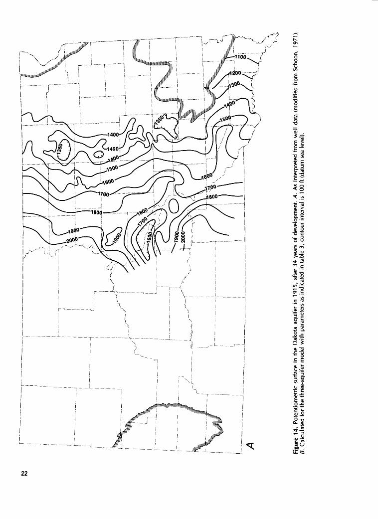
In the transient simulation, the aquifer storage coefficient and the specific storage of the confining lay­ ers were adjusted by trial-and-error until the calculated potentiometric surface was in close agreement with observed conditions in the Dakota. Schoon (1971) pres­ ents the potentiometric surface in 1914-15; this is com­ pared with the best calculated surface in figure 14.

The calculated potentiometric head following development was much more sensitive to the specific

storage in the confining layers than to the storage coeffi­ cient in the aquifer. When the specific storage in the confining beds was made small, computed drawdowns were too large even when large values for the aquifer storage coefficient were used. Figure 15 shows the com­ puted potentiometric surface after 16 years of simulated development, using the first (single-aquifer) model, for a system in which storage in the confining layer is neglected "steady" leakage with a confining layer conductivity of 5x10^" ft/sec is included in this computation. If the assumption that we could neglect the storage within the confining layer were correct, this result should approximate Darton's observations. It clearly does not.

The computed potentiometric surface could be ad­ justed to good agreement with the observed potentiome­ tric surface only when the specific storage in the confin­ ing beds was accounted for. This leads us to conclude that most of the water released from storage in the sys­ tem since development began has come from the confin­ ing beds.

Figure 10. Computed potentiometric surface for the Dakota aquifer, with an assumed hydraulic conductivity for the combined Cretaceous shale confining layer of 5 x 10~ 9 ft/sec, contours of head above land surface, contour interval is 10 ft. Heads are lower than those recorded by Darton (1909) (see figure 9).

16

Figure 11. Computed potentiometric surface for the Dakota aquifer, with an assumed hydraulic conductivity for the combined Cretaceous Shale confining layer of 5xlO~ 11 ft/sec, contours of head above land surface, contour interval is 10 ft.

Model of Cretaceous Shale Confining Layer

The analyses described above treat the Cretaceous shale confining layer as a single homogeneous unit. As seen earlier (fig. 4), this is a considerable simplification. To obtain a better understanding of the Cretaceous shale confining layer, a refined model (fourth model) was used for flow simulations. The Dakota-Newcastle Sandstone, the Greenhorn Limestone, and the Niobrara Formation were treated as aquifers and the intervening shales as confining layers. A limited number of observa­ tions of potentiometric head in the Greenhorn Lime­ stone and the Niobrara Formation exist (Steece and Howells, 1965; Stephens, 1967; Koch, 1970; Jorgenson, 1971; U.S. Geological Survey); simulation parameters were adjusted to obtain best agreement with these obser­ vations.

Actual adjustment of the parameters was accom­ plished with a nonlinear least-squares regression tech­ nique developed by S. P. Larson (written commun., 1978). The technique iteratively converges on an opti­ mum set of parameters. Optimum parameters are those which minimize S*:

S * = (10)

where 0n,0bs is the observed potentiometric head atthe nth node,

0n,caic is t*16 calculated potentiometric head atthe nth node, and

N is the number of nodes.

As in the previous model analyses, the hydraulic con­ ductivity of the Dakota was assumed to be known. The horizontal and vertical conductivities of the remaining two aquifers and three confining layers were allowed to "float" and assume their optimal values. Some difficulty was encountered with the aquifer conductivities, which tended to assume unrealistically high and low values; this results from the small number of head measure­ ments in the upper two aquifers. The aquifer transmis- sivities were arbitrarily "frozen," and the confining layer conductivities were allowed to reach their optimum values. The transmissivity of the Niobrara and the ver­ tical conductivity of the Pierre were found to be highly correlated. This means that, in the model, there was lit-

17

00

Figu

re 1

2. V

irg

in p

ote

ntio

me

tric

sur

face

fo

r th

e D

akot

a a

qu

ifer.

A,

As

map

ped

by D

arto

n (1

909

r P

late

XI).

B,

Cal

cula

ted

for

this

stu

dy u

sing

th

e t

hird

(t

hre

e-a

qu

ifer)

mo

de

l w

ith p

aram

eter

s as

ind

icat

ed i

n ta

ble

3r c

on

tou

r in

terv

al i

s 10

0 ft

(da

tum

sea

lev

el).

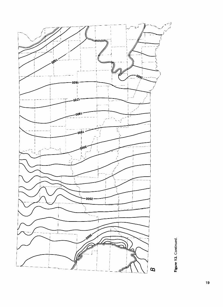
B Figu

re 1

2. C

ontin

ued.

tie difference in the computed heads when both trans- missivity in the Niobrara and conductivity in the Pierre were increased or decreased by the same factor. Because the transmissivity in the Niobrara is somewhat un­ certain, the same is true of vertical conductivity in the Pierre.

Simulation Parameters

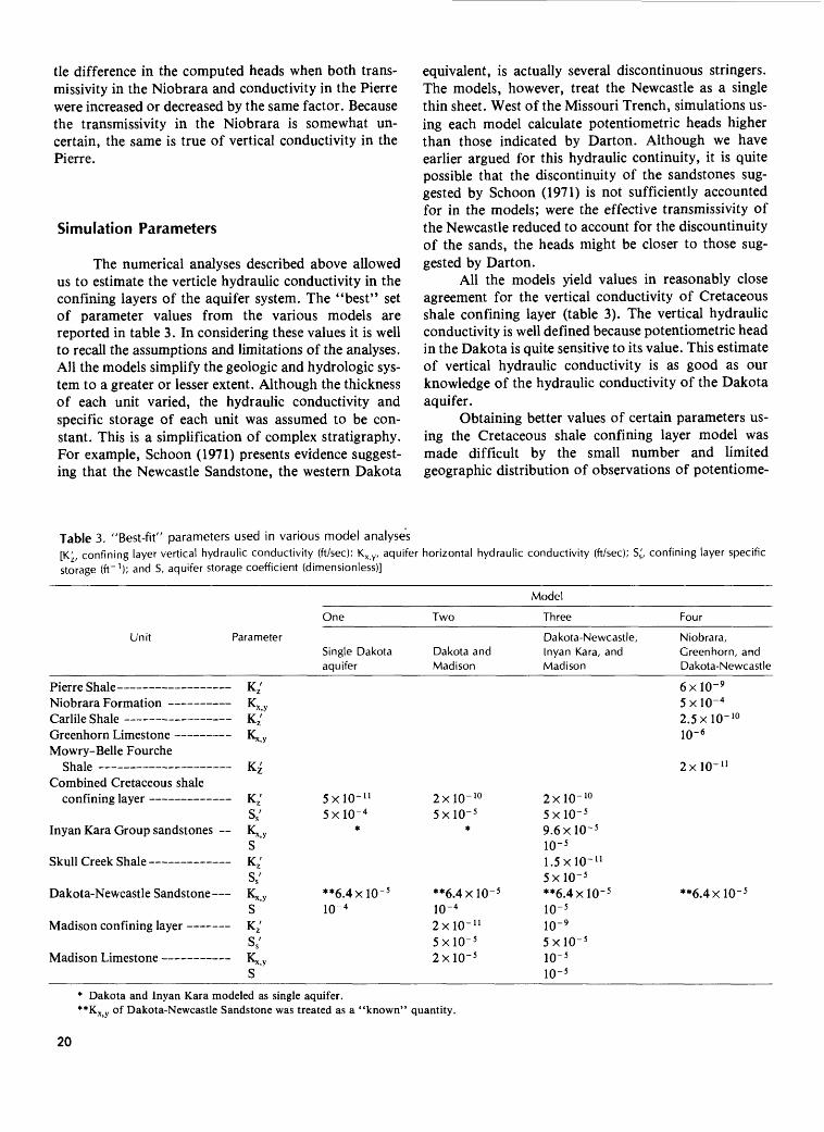
The numerical analyses described above allowed us to estimate the verticle hydraulic conductivity in the confining layers of the aquifer system. The "best" set of parameter values from the various models are reported in table 3. In considering these values it is well to recall the assumptions and limitations of the analyses. All the models simplify the geologic and hydrologic sys­ tem to a greater or lesser extent. Although the thickness of each unit varied, the hydraulic conductivity and specific storage of each unit was assumed to be con­ stant. This is a simplification of complex stratigraphy. For example, Schoon (1971) presents evidence suggest­ ing that the Newcastle Sandstone, the western Dakota

equivalent, is actually several discontinuous stringers. The models, however, treat the Newcastle as a single thin sheet. West of the Missouri Trench, simulations us­ ing each model calculate potentiometric heads higher than those indicated by Darton. Although we have earlier argued for this hydraulic continuity, it is quite possible that the discontinuity of the sandstones sug­ gested by Schoon (1971) is not sufficiently accounted for in the models; were the effective transmissivity of the Newcastle reduced to account for the discountinuity of the sands, the heads might be closer to those sug­ gested by Darton.

All the models yield values in reasonably close agreement for the vertical conductivity of Cretaceous shale confining layer (table 3). The vertical hydraulic conductivity is well defined because potentiometric head in the Dakota is quite sensitive to its value. This estimate of vertical hydraulic conductivity is as good as our knowledge of the hydraulic conductivity of the Dakota aquifer.

Obtaining better values of certain parameters us­ ing the Cretaceous shale confining layer model was made difficult by the small number and limited geographic distribution of observations of potentiome-

Table 3. "Best-fit" parameters used in various model analyses[K', confining layer vertical hydraulic conductivity (ft/sec); Kxy , aquifer horizontal hydraulic conductivity (ft/sec); Ss', confining layer specificstorage (ft" 1 ); and S, aquifer storage coefficient (dimensionless)]

Unit Parameter

Pierre Shale K2'Niobrara Formation KxyCarlile Shale Kz'Greenhorn Limestone K* y Mowry-Belle Fourche

rii_ -. 1- IT i

Combined Cretaceous shaleconfining layer Kz

0 ' as

One Two

Single Dakota Dakota and aquifer Madison

S v lO" 11 9 v 10~ 10J A L\J £ A L\J

5xlO- 4 5xlO- 5

Model

Three

Dakota-Newcastle, Inyan Kara, and Madison

A* S\. \.\J

5xlO- 5

Four

Niobrara, Greenhorn, and Dakota-Newcastle6x10 95xlO~ 4 2 S x 10~ 10^.J A ll/io- 6

*« /s. ivy

Inyan Kara Group sandstones K^s'Skull Creek Shale Kz'

s:

9.6xlO~ 5io- 5l.SxlO- 11 5xlO~ 5

Dakota-Newcastle Sandstone K^ys'

Madison confining layer K2'S s'

Madison Limestone K^ ys'

**6.4xlO- 5 **6.4xlO- 5io- 4 io- 4

2 v 10" 11{* /\ lv/

5xlO- 5^ A 1U

**6.4xlO- 5 **6.4xlO- 5io- 5 io- 95xlO- 5

io- 5* Dakota and Inyan Kara modeled as single aquifer.**KX y of Dakota-Newcastle Sandstone was treated as a "known" quantity.

20

trie head in the Niobrara and Greenhorn aquifers. This limited set of observations produces a tendency for the computed Greenhorn and Niobrara hydraulic conduc­ tivities to become unrealistic when using the nonlinear least-squares regression method of parameter estima­ tion. It also yields poorer estimates of the vertical con­ ductivities in the Pierre and Carlile Shales than for the lower Mowry-Belle Fourche Shale. As measured by the expected error, the Pierre and Carlile values are plus or minus 95 and 98 percent, respectively; the Mowry-Belle Fourche value is plus or minus only 24 percent.

It is of interest to note the trend of decreasing hydraulic conductivity with depth of burial in the Cretaceous shale confining layer (table 3). If the Skull Creek Shale below the Newcastle Sandstone is included, the conductivity appears to approach a minimum value of approximately 10 ~ n ft/sec.

In summary, the gross vertical hydraulic conduc­ tivity of the combined Cretaceous shale confining layer is well defined. However, the layer contains several shale units as well as two minor, but extensive, aquifers. There is insufficient information to define the vertical conductivities of the individual shales with precision, but the analysis indicates, as we might expect, a decrease in hydraulic conductivity with depth of burial.

Total Flow

From the numerical analysis, one can compute the total flow through each element of the system. We have made these computations for the third (three-aquifer) model. The results of summing all the flow, both in and out of the boundaries and through the confining layers, are shown in figure 16. The balance indicates that the total steady-state flow through the entire system in South Dakota was quite small, on the order of 100 ftVsec. Furthermore, most of the recharge and dis­ charge of the Dakota aquifer occurred as leakage through the confining layers, especially through the overlying Cretaceous shale confining layer.

We have chosen to treat the Paleozoic rocks beneath the Madison as impermeable in our models, thus no flow in these units is represented in figure 16. Flow occurring in these rocks would have been lumped with flow in the Madison in our analysis and thus can­ not be distinguished.

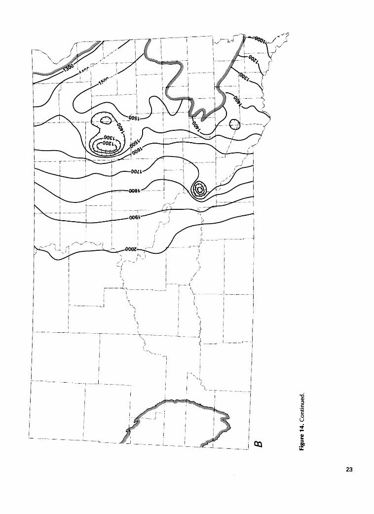
The computed steady-state areal distribution of leakage between the Dakota aquifer and the surface through the Cretaceous shale confining layer is shown in figure 17. The rates of leakage vary from zero to ap­ proximately ± 10x 10~ u ft/sec. This is equivalent to a maximum rate of ±0.04 in/yr. These are small quan­ tities of leakage; however, when one considers the large areas over which they occur, they become significant.

CRETACEOUS SHALE CONFINING LAYER: IN SITU AND LABORATORY TESTS

A number of tests have been conducted both in the field and in the laboratory in an effort to investigate further the hydraulic conductivity of the shale confining layers.

Pumping Test at Wall, South Dakota

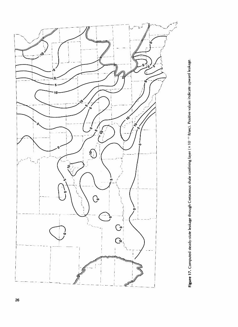
Gries and others (1976) describe one of the few carefully conducted pumping tests in the Dakota Sand­ stone. Three municipal wells in Wall, South Dakota, were utilized; one was pumped, and the others were used as observation wells. As pointed out earlier, Gries and others analyzed the results using the nonleaky solu­ tion of Theis (1935). However, the data can also be fitted to the modified solution of Hantush (1960), which in­ cludes leakage from confining layers with storage (fig. 18).

The modified Hantush solution yields a product of vertical hydraulic conductivity, Kz', and specific storage, Ss', for the confining layer. The data from both observation wells fit the modified Hantush solution and yield two different values for the product:1. K^Ss'=2.8xlO-15 secM and2. K^Ss'=1.3xlO-15 secM .The product cannot be factored using information from the test. However, if we use the simulation-derived estimate for Ss'of 5 x 10 ~ 5 ft- 1 , we obtain two values of vertical hydraulic conductivity:1. Kz'= 5.7x10-"ft/sec and2. Kz'= 2.7 x 10-» ft/sec.These values are close to those estimated for the Mowry- Belle Fourche and Skull Creek Shales in the numerical flow simulations.

Og 200 -

Figure 13. Well discharge and number of wells, Dakota aquifer in South Dakota.

21

ISJ

IS)

A

Figu

re 1

4. P

oten

tiom

etric

sur

face

in

the

Dak

ota

aqui

fer

in 1

915,

afte

r 34

yea

rs o

f de

velo

pmen

t. A

. As

int

erpr

eted

fro

m w

ell

data

(m

odifi

ed f

rom

Sch

oon,

19

71).

B. C

alcu

late

d fo

r th

e th

ree-

aqui

fer

mod

el w

ith p

aram

eter

s as

ind

icat

ed i

n ta

ble

3, c

onto

ur in

terv

al i

s 10

0 ft

(dat

um s

ea l

evel

).

B Figu

re 1

4. C

ontin

ued.

NJ

CO

Figu

re 1

5. C

om

pute

d p

ote

ntio

metr

ic s

urfa

ce i

n th

e D

akot

a aq

uife

r fo

llow

ing

16

year

s of

sim

ulat

ed d

evel

opm

ent

for

the

perio

d 18

92 t

o 1

908.

Thi

s co

mpu

tatio

n is

mad

e us

ing

the

single

-aquife

r m

odel

and

neg

lect

ing

stor

age

in t

he c

on

finin

g l

ayer

, co

ntou

r in

terv

al i

s 20

0 ft

(dat

um s

ea l

evel

).

BLACK HILLS

14.9

4-A CRETACEOUS SHALE CONFINING LAYER

64.3 36.8

SIOUX RIDGE

^LLINE*0

3&

Figure 16. Computed virgin, or steady flow, through the major elements of the aquifer system in South Dakota. Flows are summed over the entire model area; units are cubic feet per second.

Slug Tests in the Pierre Shale

Three modified slug tests (Bredehoeft and Papadopulos, 1980; Neuzil, 1982) were conducted for this investigation in a borehole located at site A in figure 19. This type of test is well suited for making in situ measurements of hydraulic properties in very low permeability rocks. A packer was set at 105 ft, and the interval from the packer to the bottom of the hole was tested. Upon completion of the first test, the packer was lowered to 210 ft and reset, and the lower portion of the hole was retested. A third test was conducted in the same manner with the packer set at 378 ft.

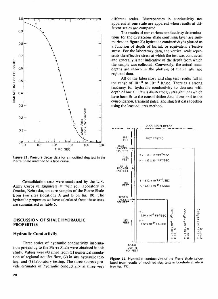
The test setup is shown schematically in figure 20. For redundancy, two separate transducers were used to record the pressure decay. An example of the test results, plotted as dimensionless head decline versus time, is shown matched to a type curve in figure 21.

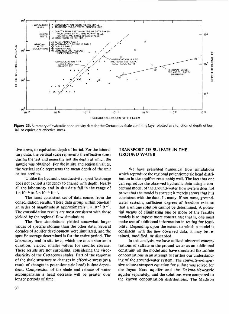
Successively shorter portions of the hole were tested; transmissivities of three separate portions of the borehole were calculated. The results of these calcula­ tions are summarized in figure 22. The data from the tests are internally consistent in that, as smaller portions of the section were tested, smaller transmissivity values were calculated. The calculated hydraulic conductivity also decreases with depth.

Bredehoeft and Papadopulos (1980) point out that the modified slug test is not without potential sources of error. During the test, very small volumes of water flow from the borehole into the rock. The possibility exists that sufficient leakage occurs through joints and con­

nections in the test apparatus or past the packer to pro­ duce an erroneous pressure decay. Leakage from the piping is particularly hard to rule out. If leakage occurs, the computed conductivity will be larger than the true conductivity of the rock.

Some evidence exists that leakage did occur in the system and that the calculated conductivities are too large. Inflation of the packers causes a small pressure rise which itself constitutes a slug test. In instances where the decay of these small pressure pulses was monitored, their decline differed from that of the full slug; the decay in this instance was slower. This suggests that the higher pressure differences associated with the full slug may have caused leakage around the packer. The actual conductivity of the rock may be lower than we have calculated.

Laboratory Pulse Tests

The usual laboratory hydraulic conductivity tests require that steady flow be established through the sam­ ple. At low values of conductivity, a long period of time is necessary to establish steady flow in a sample in which the compressive storage is significant. In addition, unless unrealistically large hydraulic gradients across the sample are used, the flow rates are small and diffi­ cult to measure. For these reasons, various investigators have attempted to utilize transient laboratory tests for low-permeability rock. An analytical solution and test methodology has been presented for a transient pulse

25

N3

O)

Figu

re 1

7. C

ompu

ted

stea

dy-s

tate

lea

kage

thr

ough

Cre

tace

ous

shal

e co

nfin

ing

laye

r (x

10-"

ft/s

ec).

Pos

itive

val

ues

indi

cate

upw

ard

leak

age.

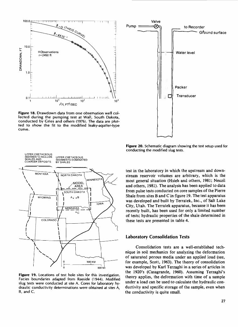
100.0

10.0 -

Valve

r2/!, FT2/SEC

Figure 18. Drawdown data from one observation well col­ lected during the pumping test at Wall, South Dakota, conducted by Cries and others (1976). The data are plot­ ted to show the fit to the modified leaky-aquifer-type curve.

Pump to Recorder""" Gfound surface

Water level

Packer

Transducer

UPPER CRETACEOUS SEDIMENTS INCLUDE SHALES AND COARSER DEPOSITS

UPPER CRETACEOUS SEDIMENTS DOMINATED BY SHALES

MODEL _,_ AREA

500 Ml

Figure 19. Locations of test hole sites for this investigation. Facies boundaries adapted from Reeside (1944). Modified slug tests were conducted at site A. Cores for laboratory hy­ draulic conductivity determinations were obtained at sites A, B, and C.

Figure 20. Schematic diagram showing the test setup used for conducting the modified slug tests.

test in the laboratory in which the upstream and down­ stream reservoir volumes are arbitrary, which is the most general situation (Hsieh and others, 1981; Neuzil and others, 1981). The analysis has been applied to data from pulse tests conducted on core samples of the Pierre Shale from sites B and C in figure 19. The test apparatus was developed and built by Terratek, Inc., of Salt Lake City, Utah. The Terratek apparatus, because it has been recently built, has been used for only a limited number of tests; hydraulic properties of the shale determined in these tests are presented in table 4.

Laboratory Consolidation Tests

Consolidation tests are a well-established tech­ nique in soil mechanics for analyzing the deformation of saturated porous media under an applied load (see, for example, Scott, 1963). The theory of consolidation was developed by Karl Terzaghi in a series of articles in the 1920's (Casagrande, 1960). Assuming Terzaghi's theory applies, the deformation with time of a sample under a load can be used to calculate the hydraulic con­ ductivity and specific storage of the sample, even when the conductivity is quite small.

27

103 1Q4

TIME, SEC

Figure 21. Pressure decay data for a modified slug test in the Pierre Shale matched to a type curve.

Consolidation tests were conducted by the U.S. Army Corps of Engineers at their soil laboratory in Omaha, Nebraska, on core samples of the Pierre Shale from two sites (locations A and B on fig. 19). The hydraulic properties we have calculated from these tests are summarized in table 5.

DISCUSSION OF SHALE HYDRAULIC PROPERTIES

Hydraulic Conductivity

Three scales of hydraulic conductivity informa­ tion pertaining to the Pierre Shale were obtained in this study. Values were obtained from (1) numerical simula­ tion of regional aquifer flow, (2) in situ hydraulic test­ ing, and (3) laboratory testing. The three sources pro­ vide estimates of hydraulic conductivity at three very

different scales. Discrepancies in conductivity not apparent at one scale are apparent when results at dif­ ferent scales are compared.

The results of our various conductivity determina­ tions for the Cretaceous shale confining layer are sum­ marized in figure 23; hydraulic conductivity is plotted as a function of depth of burial, or equivalent effective stress. For the laboratory data, the vertical scale repre­ sents the effective stress at which the test was conducted and generally is not indicative of the depth from which the sample was collected. Conversely, the actual mean depths are shown in the plotting of the in situ and regional data.

All of the laboratory and slug test results fall in the range of lO" 11 to 10- 14 ft/sec. There is a strong tendency for hydraulic conductivity to decrease with depth of burial. This is illustrated by straight lines which have been fit to the consolidation data alone and to the consolidation, transient pulse, and slug test data together using the least-squares method.

GROUND SURFACE v . ^_^f -^_- '

105 J FEET j

TEST 1 ^ PACKER * 105 FEET /

105 | FEET j

TEST 2

210 FEET

168 , FEET

TESTS

378 FEET

226 . FEET

TO DE

604

^*

-*

TA 3Th FEE

NOT TESTED

T= 1.19x 10-8 FT2/SEC

K = 1.13 x 1Q- 10 FT/SEC

T = 8.42 x 10-9 FT2/SEC

K = 5.17 x 1Q- 11 FT/SEC

T =

3.88 x 10"9 FT2/SEC

K =

1.72 x 10' 11 FT/SEC

OLU CO

OJ

LL O>

O

X ^^coco

CO COII LU

HET

OLU CO

H LL

CO

o

X

^COII LU

l-t

OLU CO

LL

CO

O

X

CVJ

IIh-

Figure 22. Hydraulic conductivity of the Pierre Shale calcu­ lated from results of modified slug tests in borehole at site A (see fig. 19).

28

Table 5. Summary of laboratory consolidation test results forthe Pierre Shale[Locations A and B refer to fig. 19]

Sample depth (ft) and corehole location

Average effective stress during test (Pa)

Hydraulic conductivity(ft/sec)

Specific storage (ft- 1 )

The hydraulic conductivities obtained from the slug tests are probably more consistent with the consoli­ dation data least-squares line values than shown in figure 23 because (1) as noted earlier, leakage during the test may have caused calculated values which are too large and (2) the slug tests measured horizontal hydraulic conductivity, whereas the other data shown in figure 23 are for vertical hydraulic conductivity. In sedimentary 108 B 1.13x10* 2.3xlO~ 12 2.0 xlO" 5 rocks, the hydraulic conductivity is generally greatest 2.29X106 7.2xlO~ 13 1.4xlQ- 5 parallel to the bedding. 4.64X106 5.9xlO~ 13 1.3xlO' 5

A least-squares line has also been fitted to the esti- 9.28 xlO6 3.3xlO~ 13 1.3xlO~ 5 mates of hydraulic conductivity obtained using the 1.59xl07 1.3xlO~ 13 1.3xlQ- 5

9 AS v 1ft7 1 9v1ft~ 13 1 3v1ft~ 5regional flow simulations. The regional values quite ^ B __________ f^J^ \ 4 * lo -n \ <*£->clearly indicate a different trend than the small-scale 2 30X106 62xl(T 13 1 5xlO~ 5laboratory and intermediate-scale slug tests; the esti- 460X106 43xlO~ 13 1 4xlO~ 5mates from the regional flow simulations are consis- 9.21 xlO6 1.8xlO~ 13 1.3xlO~ 5tently larger, generally by one to three orders of 1.57xl07 6.9xlO~ 14 l.lxlO' 5magnitude. 2.47 xlO7 6.2 xl(T 14 8.5xlO~ 6

This discrepancy between the small- and large- 233 A 2.27X106 2.0xlO~ 12 8.2xlO~ 6scale results suggests that the confining layer is probably 4.54X106 l.lxKT 12 8.2xlO~ 6fractured. The leakage observed on a regional scale 9.09xlO6 6.2xlO' 13 8.2xlO~ 6could occur largely in the fractures; however, the 1.55xl07 1.8xlO~ 13 8.5xlO~ 6hydraulic conductivities measured in the laboratory and 2 - 46 x 10? 8l9 x 10 j* 8>8 x 10 Jthe slug tests reflect the properties of the intact shale 482A 2.30x10* 5.3x10^ 4.0x10^

between fractures. 9 '21xl06 66xlQ-" 40xlO~ 6The pumping test at Wall yielded values compara- 1 57xl07 12xlO~ 13 40xlO~ 6

ble with those of the regional model analysis (fig. 23). 2 47x 107 4 3 x 10~ 13 4 Ox 10~ 6This indicates that the pumping test may have been in- 102 A______ 2.31 x 106 4.6 x 10~ 12 1.2x 10~ 5fluenced by leakage from fractures in the confining 4.64X106 7.2xlO~ 12 1.2xlO~ 5layer. During the 44-hr duration of the test, the cone of 9.37X106 1.4xlO~ 12 1.3xlO~ 5depression spread out to a radius of 6 mi from the 1.60xl07 3.6xlO~ 13 1.3xlO~ 5pumped well, suggesting that the fracture spacing in the 2.48xlO7 3.0X10' 13 1.4xlO- 5confining layer is on the order of miles or less. 45° B 2 -27 x 1Q6 3- 1 x 10~ j' 9 -4 x 10^

The scatter present in the laboratory data prob- 4.54X106 2.7x10 | 2 9.8xlOjably results from measurement error, not lithologic dif- 9 '°? x }^ 6 '9x |J" 13 j^ x ]° ~ 5ferences in the samples. Small hydraulic conductivities 2 45 x 107 23 x 10' 13 1 1 x 10' 5are difficult to measure, and resolution of such small 125 A_____ 2 32X106 69xlO~ 13 1 IxlO" 5values to significantly better than order-of-magnitude 464X106 43xlO~ 13 llxlO~ 5may not be possible. 9.28xlO6 3.2xlO' 13 1.2xlO- 5

1.58X107 1.3X10" 13 1.3xlO- 52.47 XlO7 9.2X10' 14 1.3X10' 5

364 A 5.83 xlO5 1.6X1Q-' 1 1.4X1Q- 5

Table 4. Summary of laboratory transient pulse test results 1.17x10* 5.3x10' 1.4x10-for the Pierre Shale 2.32x10* 2.0xlO' 12 7.6XHT 6[Locations B and C refer to fig. 19] 4.64X106 1.3xlO' 12 7.6X10" 6

___________________________________ 9.28X106 5.6xlO' 13 7.9xlO~ 6Sample depth 1.59xl07 9.5xlO' 14 7.9X10" 6(ft) and Effective stress Hydraulic Specific 2.48X107 8.2xlO~ 14 8.2xlO~ 6 corehole during test conductivity storage location_______(Pa)_________(ft/sec)______(ft- 1 )

144C 3.75X106 l.3xio- 12 9.4xiQ- 7 Specific Storage 6.06 xlO6 1.3 xlO' 12 4.0 xlO- 6

148C 1.28xlO7 1.1 xlO- 12 2.5xlO" 6 The specific storage of the confining layer was171 C 1.08xlO7 2.6xlO- 12 1.3xlO- 6 also determined by all the methods of analysis; these

9.90 x 106 3.0 x 10" 12 1.3 x 10" 6 results are summarized in figure 24. As with the hydraulic367B 1.27xlO7 6.6xlQ- 12 2.4xlO" 7 conductivity data, the results are plotted against effec-

29

1U~

PASCALS

4

CO LU CC

r~ 0

LS 3AI1O3:

LJ_LL LU

108

1C

LABORATORY I CONSOLIDATION TESTS, PIERRE SHALE TESTS | * TRANSIENT 'PULSE' TESTS, PIERRE SHALE

I A DAKOTA PUMP TEST (ANALYSIS OF DATA TAKEN FROM CRIES ET AL, 1976) MOWRY-BELLE . FOURCHE AND SKULL CREEK SHALES /

Q SLUG TESTS, PIERRE SHALE /

( © SKULL CREEK SHALE , /^ a REGIONAL 1 © MOWRY-BELLE FOURCHE SHALE / /' *

FLOW { © CARLILE SHALE / / SIMULATIONS © PIERRE SHALE ' / n

{ © COMBINED CRETACEOUS . / / CONFINING LAYER * / ?

'' / ^CONSOLIDATION, 'PULSE' ^^~-~®~~ CONSOLIDATION * / / * * AND 'SLUG 1 TEST DATA, _, -"

DATA, LEAST- _______ / / LEAST-SQUARES FIT -_, _^ - -~~ SQUARES FIT ~~~~^' , ^ ^^-^^^

. | . / *. . __---^" @ ^REGIONAL MODEL f / -. ^-^~~^ ESTIMATES, LEAST-

/ ' * ^.?--^~~^~~'^ SQUARES FIT

/ / x x/ / * X

/

% */' * * *

1 1 1 ,1 1 1 , 1

102

LL

_f

CC

DEPTH OF

10 4

-14 10-13 10-12 1Q-11 10-10 10-9 10-8

HYDRAULIC CONDUCTIVITY, FT/SEC

Figure 23. Summary of hydraulic conductivity data for the Cretaceous shale confining layer plotted as a function of depth of bur­ ial, or equivalent effective stress.

tive stress, or equivalent depth of burial. For the labora­ tory data, the vertical scale represents the effective stress during the test and generally not the depth at which the sample was obtained. For the in situ and regional values, the vertical scale represents the mean depth of the unit or test section.

Unlike the hydraulic conductivity, specific storage does not exhibit a tendency to change with depth. Nearly all the laboratory and in situ data fall in the range of Ixl0- 6 to2xl0- 5 ft- 1 .

The most consistent set of data comes from the consolidation results. These data group within one-half an order of magnitude at approximately 1 x 10~ 5 ft" 1 . The consolidation results are most consistent with those yielded by the regional flow simulations.

The flow simulations yielded somewhat larger values of specific storage than the other data. Several decades of aquifer development were simulated, and the specific storage determined is for the entire period. The laboratory and in situ tests, which are much shorter in duration, yielded smaller values for specific storage. These results are not surprising, considering the visco- elasticity of the Cretaceous shales. Part of the response of the shale structure to changes in effective stress (as a result of changes in potentiometric head) is time depen­ dent. Compression of the shale and release of water accompanying a head decrease will be greater over longer periods of time.

TRANSPORT OF SULFATE IN THE GROUND WATER

We have presented numerical flow simulations which reproduce the regional potentiometric head distri­ bution in the aquifers reasonably well. The fact that one can reproduce the observed hydraulic data using a con­ ceptual model of the ground-water flow system does not prove that the model is correct; it merely shows that it is consistent with the data. In many, if not most, ground- water systems, sufficient degrees of freedom exist so that a unique solution cannot be determined. A poten­ tial means of eliminating one or more of the feasible models is to impose more constraints; that is, one must make use of additional information in testing for feasi­ bility. Depending upon the extent to which a model is consistent with the new observed data, it may be re­ tained, modified, or discarded.

In this analysis, we have utilized observed concen­ trations of sulfate in the ground water as an additional constraint on the model and have simulated the sulfate concentrations in an attempt to further our understand­ ing of the ground-water system. The convective-disper- sive solute-transport equation for sulfate was solved for the Inyan Kara aquifer and the Dakota-Newcastle aquifer separately, and the solutions were compared to the known concentration distributions. The Madison

30

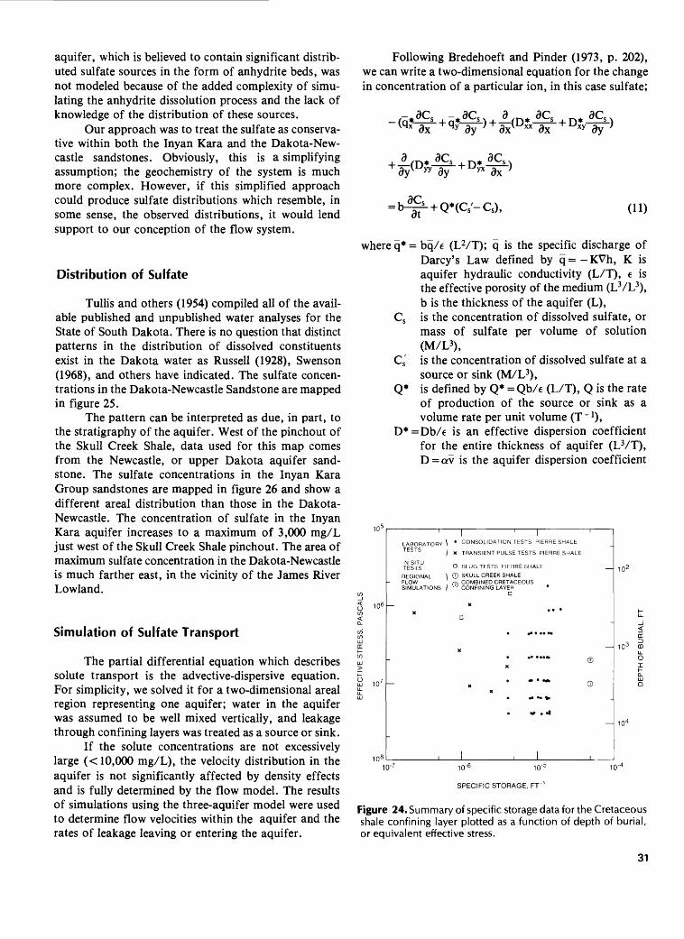
aquifer, which is believed to contain significant distrib­ uted sulfate sources in the form of anhydrite beds, was not modeled because of the added complexity of simu­ lating the anhydrite dissolution process and the lack of knowledge of the distribution of these sources.

Our approach was to treat the sulfate as conserva­ tive within both the Inyan Kara and the Dakota-New­ castle sandstones. Obviously, this is a simplifying assumption; the geochemistry of the system is much more complex. However, if this simplified approach could produce sulfate distributions which resemble, in some sense, the observed distributions, it would lend support to our conception of the flow system.

Distribution of Sulfate

Tullis and others (1954) compiled all of the avail­ able published and unpublished water analyses for the State of South Dakota. There is no question that distinct patterns in the distribution of dissolved constituents exist in the Dakota water as Russell (1928), Swenson (1968), and others have indicated. The sulfate concen­ trations in the Dakota-Newcastle Sandstone are mapped in figure 25.

The pattern can be interpreted as due, in part, to the stratigraphy of the aquifer. West of the pinchout of the Skull Creek Shale, data used for this map comes from the Newcastle, or upper Dakota aquifer sand­ stone. The sulfate concentrations in the Inyan Kara Group sandstones are mapped in figure 26 and show a different areal distribution than those in the Dakota- Newcastle. The concentration of sulfate in the Inyan Kara aquifer increases to a maximum of 3,000 mg/L just west of the Skull Creek Shale pinchout. The area of maximum sulfate concentration in the Dakota-Newcastle is much farther east, in the vicinity of the James River Lowland.

Simulation of Sulfate Transport

The partial differential equation which describes solute transport is the advective-dispersive equation. For simplicity, we solved it for a two-dimensional areal region representing one aquifer; water in the aquifer was assumed to be well mixed vertically, and leakage through confining layers was treated as a source or sink.

If the solute concentrations are not excessively large (< 10,000 mg/L), the velocity distribution in the aquifer is not significantly affected by density effects and is fully determined by the flow model. The results of simulations using the three-aquifer model were used to determine flow velocities within the aquifer and the rates of leakage leaving or entering the aquifer.

Following Bredehoeft and Finder (1973, p. 202), we can write a two-dimensional equation for the change in concentration of a particular ion, in this case sulfate;

A(D*_^dy yy dy

dCs

dx

+ Q*(CS'-CS), (11)

where q* = bq/e (L2/T); q is the specific discharge of Darcy's Law defined by q = - KVh, K is aquifer hydraulic conductivity (L/T), e is the effective porosity of the medium (L3 /L3), b is the thickness of the aquifer (L),

Cs is the concentration of dissolved sulfate, or mass of sulfate per volume of solution (M/L3),

Cs' is the concentration of dissolved sulfate at a source or sink (M/L3),

Q* is defined by Q* = Qb/e (L/T), Q is the rate of production of the source or sink as a volume rate per unit volume (T~ ! )»

D*=Db/e is an effective dispersion coefficient for the entire thickness of aquifer (L3/T), D = av is the aquifer dispersion coefficient

106

LABORATORY \ TESTS i

REGIONALFLOWSIMULATIONS

CONSOLIDATION TESTS PIERRE SHALE

X TRANSIENT PULSE TESTS PIERRE SHALE

O SLUG TESTS PIERRE SHALE

© SKULL CREEK SHALEfj, COMBINED CRETACEOUSw CONFINING LAYER *

10" 10-' 10"' 10"

SPECIFIC STORAGE, FT~

Figure 24. Summary of specific storage data for the Cretaceous shale confining layer plotted as a function of depth of burial, or equivalent effective stress.

31

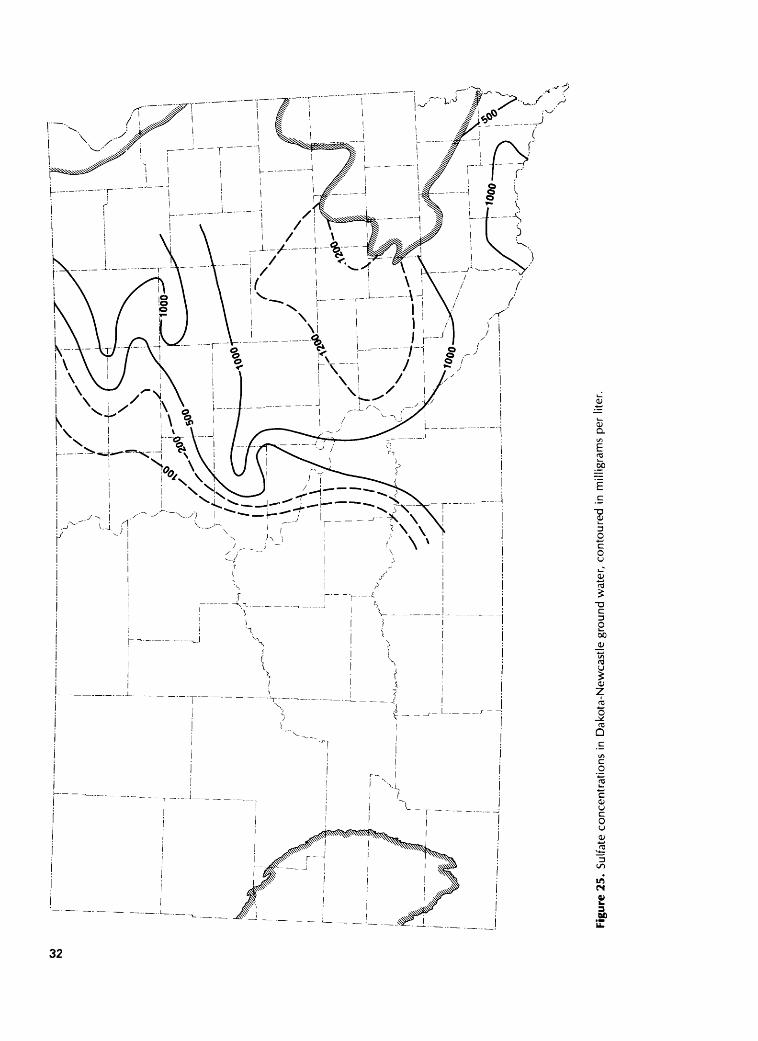
CO

NJ

Figu

re 2

5. S

ulfa

te c

on

cen

tra

tion

s in

Dak

ota-

New

cast

le g

roun

d w

ater

, co

nto

ure

d i

n m

illig

ram

s pe

r lit

er.

Figu

re 2

6. S

ulfa

te c

once

ntra

tions

in

Inya

n K

ara

grou

nd w

ater

, co

nto

ure

d i

n m

illig

ram

s pe

r lit

er.

CO

CO

(L2/T), a is the dispersivity (L), v = q/e is the average ground-water velocity (L/T).

Equation 11 was solved by using the finite-element computer program ISOQUAD (Finder, 1974) using square linear elements. The nodal spacing (approx­ imately 16.6 mi) was exactly double that used in flow models one, two and three and identical with that in flow model four. As noted above, the sulfate transport was simulated separately in the Dakota and Inyan Kara aquifers; the Dakota model consisted of 320 nodes and 275 elements, while the Inyan Kara model had 286 nodes and 245 elements.

Additional boundary conditions are required to solve the transport equation. At the outcrops in the Black Hills areas of recharge, the concentration was fixed at the value observed in the aquifer in the vicinity of the outcrop. A second type of boundary condition, zero-concentration gradient, was imposed at the zone of discharge from the Dakota outcrops in the east; this allowed the sulfate to leave the aquifer only through advection. The concentration of incoming leakage was assumed to be known and that of outgoing leakage was assumed to be equal to the aquifer fluid concentration at the point where leakage occurs. The sandstones them­ selves were assumed to be free of sulfate sources or sinks. This means that there was neither solution nor precipitation of the sulfate; mass transfer between the li­ quid and solid phases was assumed to be negligible.

Sulfate Transport in the Inyan Kara Group Sandstones

The steady-state concentrations of sulfate in the Inyan Kara were computed using the mass transport numerical simulations in conjunction with the results of the flow simulations. Hydraulic conductivity and thick­ ness of the aquifer were as defined for the three-aquifer flow model. The porosity was assigned a value of 0.20. The transverse and longitudinal dispersivities of the medium were arbitrarily set equal to 75 ft; later simula­ tions demonstrated that, at this scale, the calculated concentrations are extremely insensitive to the disper­ sivity values. The sulfate concentration in leakage from below the aquifer was taken to be 1,500 mg/L. This high value is consistent with the water chemistry of the Madison and, more importantly, with the presence of anhydrite in the intervening confining layer. Both the Spearfish and the Minnelusa Formations, which are part of the confining layer overlying the Madison aquifer, have bedded anhydrite in western South Dakota (fig. 27). It is expected that the geochemistry of the confining layer will be reflected in the leakage to the Inyan Kara from below to a greater extent than will the

water chemistry of the Madison; for this reason, a uniform concentration was assigned to the leakage.

The computed Inyan Kara sulfate concentrations are shown in figure 28. Considering the simplicity of the assumptions concerning the source of the sulfate, the results appear to us to be satisfactory. How good the fit is between observed (fig. 26) and calculated (fig. 28) concentrations is a matter of judgement. A number of other conceptual sources for the sulfate were tried. Only the system in which the source of the sulfate was leakage from below gave results even approaching the observed distribution. The chief discrepancies of the computed concentrations are a lower east-west concentration gra­ dient and an absence of the regional high in the west- central area. If the basic conceptual model of the system is correct, these differences could easily be accounted for by areal variations in the chemical composition of the leakage from the Madison confining layer. This result only indicates that the source of the sulfate in the Inyan Kara is not inconsistent with our concept of the flow system.

Sulfate Transport in the Dakota-Newcastle Sandstone

Again using the results of the flow simulations to determine the velocity and leakage distributions, the steady-state sulfate concentrations in the Dakota-New­ castle were calculated. The transverse and longitudinal dispersivities were initially given the value of 75 ft, and the porosity was assumed to be 0.20. Leakage from below the Dakota was assumed to have a concentration equal to the observed value in the Inyan Kara at the point of upward leakage (see fig. 26). Leakage from the shales overlying the Dakota was assumed to have a sulfate concentration of 100 mg/L.

The dominance of advective over dispersive trans­ port was demonstrated when different dispersivity values were tried in the simulations. Even when the dis­ persivity was made as large as 2 x 104 ft, computed con­ centrations did not change substantially. The large dis­ persivities had the advantage of damping "overshoot" and "undershoot" errors (Finder and Gray, 1977) which occur where concentration gradients change rapidly. Thus, we present the concentrations in the Dakota-Newcastle computed with a very large (2 x 10" ft) dispersivity (fig. 29).

The computed concentrations correctly reproduce the general east-west gradient. In addition, the regional high in the computed values is located just northwest of the Sioux Ridge, a result which is in general agreement with the field data (fig. 25). South of the Sioux Ridge, in the southeast corner of the model area, concentrations decrease due to dilution by recharge from the surface.

34

Figu

re 2

7. A

real

dis

trib

utio

n o

f gy

psum

and

an

hyd

rite

in

the

Min

nelu

sa a

nd S

pear

fish

For

mat

ions

(pa

rts o

f th

e M

adis

on c

on

finin

g l

ayer

) an

d th

e M

issi

ssip

pian

roc

ks

wh

ich

com

prise

the

Mad

ison

Gro

up (

mod

ified

fro

m S

outh

Dak

ota

Geo

logi

cal

Sur

vey,

196

4).

CO en

CO

OJ

r ..

-. .

_-_

.._

.._

.._

.._

.._

.._

.._

.._

._._

._..

_._

.._

.._

.._

.._

.._

i I

^

! J

:'\

^^^

^v

1 i

t _i

_ .

/^

x

/ <

A T

/

! \

h ,

|

^

\

s

\ \

; /

N; x

i/

i \

i '

1 (

\

'

1 ! ! i

i1

L - -n

I !

j I

i !

i !

i

- -

Figu

re 2

8.C

alc

ula

ted

sul

fate

con

cent

ratio

ns f

or I

nyan

Kar

a gr

ound

wat

er,

cont

oure

d in

mill

igra

ms

per

liter

.

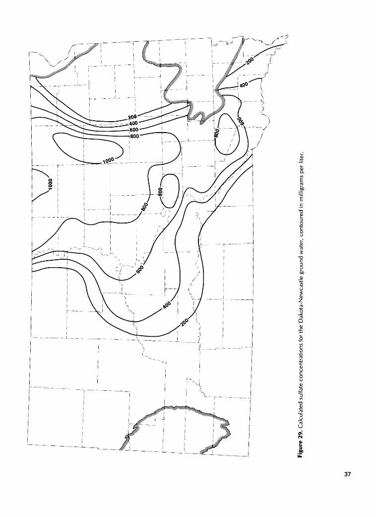
Fig

ure

29.

Cal

cula

ted

sulfa

te c

once

ntra

tions

for

the

Dak

ota-

New

cast

le g

roun

d w

ater

, co

nto

ure

d i

n m

illig

ram

s pe

r lit

er.

CO -vl

This is also expected from the observed data. The same phenomenon appears to occur north of the Sioux Ridge, although there are no observations either to confirm or to refute this possibility.

Two deficiencies of the computed values are ob­ vious. A region of concentrations as high as 600 to 800 mg/L appears west of the Missouri River; in this area, the observed concentrations are less than 100 mg/L. In the eastern part of the State, north of the Sioux Ridge, dilution of the Dakota water occurs farther west than the field data indicate.

The most serious error in the computed values is the area of fairly high concentrations west of the Missouri River. In this regard, it is important to review the assumptions associated with our simulations. The source of this excess sulfate is the steady-state upward leakage through the Skull Creek Shale; this leakage is assumed to have a sulfate concentration equal to that of water in the underlying Inyan Kara Group (fig. 26). Fur­ thermore, it is assumed that the leakage rates are deter­ mined by the equation of flow, independent of the dis­ tribution of sulfate in the ground-water system.

It is pertinent to question whether the system has reached steady state with respect to concentration (we define steady state as dCs/dt = 0), or whether it could still be in a transient state with respect to concentration of dissolved species (dCs/dt^O).

If a transient state exists, a sulfate front might be advancing upward through the Skull Creek Shale. In the east, where the shale is either thin or absent, the sulfate would have broken through into the Dakota. Farther west, where the Skull Creek Shale thickens and leakage rates are lower, the front would still be within the shale beds, having not yet reached the Dakota Sandstone. Because our simulations are for steady-state conditions, discrepancies between computed and observed concen­ trations might be partially due to the existence of a tran­ sient state in the ground-water system with respect to dissolved species.

We have made a simple calculation to examine the question of transient conditions with respect to concen­ tration. The results of mercury injection tests suggest that the Cretaceous shale has an effective porosity which ranges from 0.04 to 0.10. Leakage rates calcu­ lated using the flow model are on the order of 10~ n ft/sec which corresponds to an average water velocity of 10~ 10 ft/sec, assuming an effective porosity of 0.1. The average traveltime for leakage from the Inyan Kara to the Dakota is then equal to the thickness of the shale divided by this velocity; for a 300-ft thickness, the traveltime is estimated to be 3 x 10 12 sec, or approxi­ mately 100,000 years. Had we assumed an effective porosity of 0.01, the estimated traveltime would be approximately 10,000 years. The present tectonic setting existed in Oligocene time, or approximately 25 million

years ago (Eardley, 1962). This would suggest that the boundary conditions and, therefore, the flow system have existed in something like their present form for ap­ proximately 25 million years and that steady-state con­ ditions with respect to concentration exist.

However, if flow through the confining layers is dominantly in fractures, the traveltimes could be signifi­ cantly more than the calculation above indicates. Grisak and Pickens (1980) and Neretnieks (1980) have shown that the transport of dissolved species through fractures can be significantly retarded by diffusion into the inter- granular pores along the fracture walls. In effect, the dissolved constituent is stored in the rock matrix near the fracture walls. Under these circumstances the solute may not yet have "broken through," even though flow through the fractures has been occurring for a long period of time. In addition, short-duration changes in the boundary conditions may have occurred during Pleistocene glaciation; dissolved species concentrations could still be adjusting to these relatively recent changes.

The Role of Geological Membranes in the Transport of Sulfate

A potential weakness of the mass transport models suggested so far is their failure to consider all of the physical and chemical phenomena which govern transport. The electrical properties of clay minerals make it possible for clay and shale layers to behave as semipermeable membranes (Hanshaw and Hill, 1969; Kharaka and Berry, 1973). The effect influences both fluid flow and mass transport. A difference in concen­ tration across the membrane results in an osmotic pres­ sure difference which will affect the fluid flow. The membrane will tend to build and maintain concentra­ tion differences as a result of solute filtering. An experi­ mental investigation of this filtering by Kharaka and Berry (1973) yielded influent-effluent sulfate concentra­ tion ratios of about 2.0 for a thin bentonite filter at 8,000 lb/in2 compaction pressure.

Bredehoeft and others (1963) developed an ana­ lytical model to simulate mass transport in a system con­ taining a geological membrane and used the model to show that the membrane effect might be responsible for the concentration of brines in the Illinois basin. It is possible that the Cretaceous shales in this study behave as semipermeable membranes, or as a series of mem­ branes, and, as such, affect significantly the distribution of sulfate in the system.

To test the effect of the filtration phenomenon on sulfate transport in the system, several simplifying assumptions were made. No rigorous justifications for these assumptions are offered. It is expected, however,

38

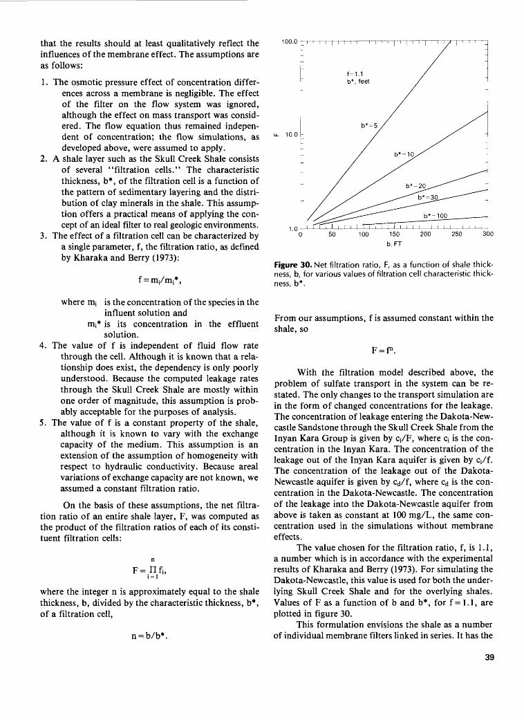
that the results should at least qualitatively reflect the influences of the membrane effect. The assumptions are as follows:

1. The osmotic pressure effect of concentration differ­ ences across a membrane is negligible. The effect of the filter on the flow system was ignored, although the effect on mass transport was consid­ ered. The flow equation thus remained indepen­ dent of concentration; the flow simulations, as developed above, were assumed to apply.

2. A shale layer such as the Skull Creek Shale consists of several "filtration cells." The characteristic thickness, b*, of the filtration cell is a function of the pattern of sedimentary layering and the distri­ bution of clay minerals in the shale. This assump­ tion offers a practical means of applying the con­ cept of an ideal filter to real geologic environments.

3. The effect of a filtration cell can be characterized by a single parameter, f, the filtration ratio, as defined by Kharaka and Berry (1973):

f = mi/mi *,

where m; is the concentration of the species in theinfluent solution and

mj* is its concentration in the effluent solution.

4. The value of f is independent of fluid flow rate through the cell. Although it is known that a rela­ tionship does exist, the dependency is only poorly understood. Because the computed leakage rates through the Skull Creek Shale are mostly within one order of magnitude, this assumption is prob­ ably acceptable for the purposes of analysis.

5. The value of f is a constant property of the shale, although it is known to vary with the exchange capacity of the medium. This assumption is an extension of the assumption of homogeneity with respect to hydraulic conductivity. Because areal variations of exchange capacity are not known, we assumed a constant filtration ratio.

On the basis of these assumptions, the net filtra­ tion ratio of an entire shale layer, F, was computed as the product of the filtration ratios of each of its consti­ tuent filtration cells:

F=nfif1 = 1

where the integer n is approximately equal to the shale thickness, b, divided by the characteristic thickness, b*, of a filtration cell,

n = b/b*.

100.0

u- 10.0 -

300

Figure 30. Net filtration ratio, F, as a function of shale thick­ ness, b, for various values of filtration cell characteristic thick­ ness, b*.

From our assumptions, f is assumed constant within the shale, so

= fn .

With the filtration model described above, the problem of sulfate transport in the system can be re­ stated. The only changes to the transport simulation are in the form of changed concentrations for the leakage. The concentration of leakage entering the Dakota-New­ castle Sandstone through the Skull Creek Shale from the Inyan Kara Group is given by cj/F, where q is the con­ centration in the Inyan Kara. The concentration of the leakage out of the Inyan Kara aquifer is given by c/f. The concentration of the leakage out of the Dakota- Newcastle aquifer is given by Cd/f, where Cd is the con­ centration in the Dakota-Newcastle. The concentration of the leakage into the Dakota-Newcastle aquifer from above is taken as constant at 100 mg/L, the same con­ centration used in the simulations without membrane effects.

The value chosen for the filtration ratio, f, is 1.1, a number which is in accordance with the experimental results of Kharaka and Berry (1973). For simulating the Dakota-Newcastle, this value is used for both the under­ lying Skull Creek Shale and for the overlying shales. Values of F as a function of b and b*, for f = 1.1, are plotted in figure 30.

This formulation envisions the shale as a number of individual membrane filters linked in series. It has the

39

Figu

re 3

1. C

alcu

late

d su

lfate

con

cent

ratio

ns f

or th

e D

akot

a-N

ewca

stle

gro

und

wat

er,

cont

oure

d in

mill

igra

ms

per

liter

; m

embr

ane

filitr

atio

n is

incl

uded

.

Figu

re 3

2. C

hlo

rid

e c

once

ntra

tions

in

Dak

ota-

New

cast

le g

roun

d w

ater

, co

nto

ure

d i

n m

illig

ram

s pe

r lit

er.

nice property that, as the shale thickens, the membrane improves in net efficiency. It has the disadvantage that the characteristic filtration cell thickness, b*, is unknown and, in our case, must be determined by trial and error.

The transport of sulfate was computed for the Dakota-Newcastle aquifer with the membrane effects included, as discussed above; the results are shown in figure 31. Adding the effects of filtration lowers the calculated concentrations west of the Missouri River; in general, we believe it improved the solution.

The calculated solution is sensitive to the value of b*. For large values of b*, the shale is a rather ineffi­ cient filter. For small values of b*, the shale is an effec­ tive filter even where it is very thin. The value which gave the best results is b* equal to approximately 20 ft.

CHLORIDE IN THE GROUND WATER

The chloride concentrations in the Dakota-New­ castle aquifer are mapped in figure 32. The distribution of chloride within the aquifer is puzzling. There is little doubt that flow occurs from west to east through the aquifer. With this flow system, it is difficult to under­ stand the concentration of chlorides that remains near the center of the flow system. The higher chloride con­ tent appears to be related to the structural axis of the Williston Basin. Several efforts to simulate the chloride concentrations were unsuccessful.

DISCUSSION

We approached this study with the deductive hypothesis, or bias if you like, that leakage through the shale confining layers forms a significant, if not domi­ nant, element of the Dakota flow system. This is not a new idea; as pointed out in the introduction, both Chamberlin (1885) and Darton (1909) expressed ver­ sions of this concept around the turn of the century. We have attempted to test the validity of this hypothesis using presently available quantitative techniques. In the process, we have estimated, within reasonable limits, numerical values for the parameters which describe the system. Indeed, the analysis has led to interesting ideas and speculations about shale confining layers.

Some data, most notably the chloride distribution in the Dakota-Newcastle aquifer, remain to be explained. However, this appears to reflect our poor understanding of certain details of the aquifer system and the geo­ chemistry. We believe that, with this exception noted, the flow system we have hypothesized is consistent with the data as we have interpreted them.

We have not validated the hypothesis, we have simply not invalidated it an important philosophical distinction. The scientific philosopher K. R. Popper, in 1959 argued in his book, The Logic of Scientific Dis­ covery, that scientific laws, theories, and hypotheses cannot be validated, they can only be "falsified" or in­ validated. We concur with Popper's view of science on this point. Accepting this viewpoint leads to the outlook that one cannot validate a particular model; one can only answer the question, is the model consistent with the data? Indeed, there may be other models which are also consistent with the data. How one views the data depends upon his model, or hypothesis, of how the system operates.

The pumping test at Wall, South Dakota, illus­ trates our point. An analysis of the Wall results using the Theis assumptions no flow through the confining layers indicates that the data are consistent with this hypothesis, within experimental error, for the period of time the test was conducted; that is, 44 hr (Gries and others, 1976). The same data are also consistent with an analysis based upon the modified leaky aquifer theory of Hantush (1960) which includes both flow and storage in the confining layers, as was pointed out above. The duration of the Wall pumping test was not sufficient to invalidate the hypothesis of leakage at the rates which the numerical simulations indicate; in that context, the experiment was not definitive. The pertinent point is that neither analysis is wrong; they simply depend upon the deductive hypothesis one believes is more appropriate.

It would be foolish on our part to believe that we have written the last word concerning the Dakota aquifer system. As N. Wood Bass, a distinguished geologist with the U.S. Geological Survey, stated, "any geological report is simply a progress report." Popper (1959) also states the same conclusion:

"The game of science is, in principle, without end. He who decides one day that scientific statements do not call for any further test, and that they can be regarded as finally verified, retires from the game."

Simplifying Assumptions

In making our analyses we have made quite a number of important simplifying assumptions. We have assumed:1. The aquifers which control the flow are the Dakota,

which we subdivided in the western part of the study area into the Inyan Kara Group sandstones and overlying Dakota-Newcastle Sandstone, and the underlying Madison Group limestones.

2. The confining layers can be idealized into those which separate the principal aquifers. This is cer­ tainly a major simplification; the confining layers,

42

as defined by us, contain a number diverse litho- Ipgic units. This is particularly true for the con­ fining layer that separates the Dakota from the Madison. Our analysis of the confining layer which overlies the Dakota indicated that this unit is more complex hydrologically than our earlier models allowed.

3. Single values of the hydraulic parameters characterize the various units of the system: hydraulic con­ ductivity, specific storage, porosity, filtration ratio, and characteristic filtration cell dimension. For the numerical simulations, the geometry of the geologic setting and the thickness of confining lay­ ers and aquifers were included in our analyses.

4. The flow and solute transport were in steady state prior to development.

5. No sulfate sources or sinks are present in the Inyan Kara Group, the Skull Creek Shale, or the Dakota- Newcastle Sandstone.

6. Membrane phenomena may affect solute transport but do not affect the ground-water flow. Even with these rather restrictive simplifying

assumptions the results are surprisingly consistent with the observations. The fact that we can make these simplifying assumptions and still get reasonable results is encouraging.

CONCLUSIONS

There are a number of interesting conclusions which stem from the investigation:1. Our analysis indicates that under steady-state condi­

tions leakage through the shale confining layers was the most important component of the flow system (see fig. 16).

2. To account for the rather small drawdown which has accompanied development of the Dakota, our analysis indicates that most of the water released from storage must have been derived from the confining layers.

3. Comparison of the hydraulic conductivity values derived from regional model analyses with the in situ and laboratory determinations suggests that much of the flow through the Cretaceous shale confining layers probably occurs as flow through fractures.

4. Upward leakage from lower units is the predominant source of sulfate in the Inyan Kara and Dakota aquifers. The calculated sulfate concentration dis­ tributions are consistent with those observed. These results art consistent with Swenson's (1968) concept of flow in the system. Our analysis further suggests that, of the approximately 80 ftVsec

which was discharged from the Dakota system under virgin conditions, about 25 percent came from the Madison aquifer (see fig. 16).

ACKNOWLEDGMENTS

This investigation has had a long and checkered history. The principal investigator joined the U.S. Geo­ logical Survey in 1962 to work with Robert R. Bennett on a study of the hydrodynamics of the Tensleep Sand­ stone in the Big Horn Basin of Wyoming. It was from that investigation that many of the ideas concerning regional flow systems, especially the role of thick shale confining layers, were formulated. An analysis of the Tensleep flow system was attempted using an electric analog model; unfortunately, the results of that analysis were not published.

Swenson's (1968) paper stimulated more thinking about regional flow, this time in the Dakota aquifer. Flow in the Dakota became the subject of a graduate seminar in ground-water hydrology which the principal investigator taught as a visiting professor at the Univer­ sity of Illinois in 1968. As part of that seminar, the class visited South Dakota where we met Martin Sather, a driller in Presho, South Dakota. Mr. Sather generously allowed us to examine the records of the Norbeck and Hollis Drilling Company, records which provided inval­ uable information concerning the hydraulic conductiv­ ity of the Dakota aquifer.

The seminar at the University of Illinois resulted in the early simplified model of the system, a model which included only the Dakota aquifer. A manuscript, in which the seminar members R. T. Getzen, M. R. McComas, R. Piskin, P. C. Rao, C. A. Rodriques, and C. H. Simonds participated, described the early model analysis; this manuscript was distributed widely for review. Among the reviewers were S. W. Lohman and F. A. Swenson. The reviews pointed out weaknesses in the early analysis. Among the weaknesses were that the analysis did not include the Madison aquifer and that it hypothesized an explanation for the sulfate in the Dakota which could not be supported when one exam­ ined that data more carefully.

Further, more detailed analysis required more sophisticated multiaquifer digital models than were available in 1968. For that reason, and the press of other work, the study languished.

Carolyn Showers, an undergraduate at Princeton University, developed a multiaquifer flow model of the system which included the Madison aquifer, while working at the U.S. Geological Survey during summer 1976. Christopher Milly, also an undergraduate at Princeton, built on Carolyn's model and added trans-

43

port while working at the Survey during the following summer. Chris used the analysis of the Dakota aquifer, in particular the analysis of sulfate distribution, for his undergraduate thesis at Princeton.

During 1978, we drilled a series of test holes in South Dakota to better define the nature of the confin­ ing layer. Christopher Neuzil joined the staff of the project in 1978 and participated in the field and labora­ tory experiments. Chris used an analysis of toxic waste disposal in the Cretaceous shale for the subject of his Ph.D. dissertation in geology at Johns Hopkins Univer­ sity, a dissertation he completed in 1980.

All of these individuals, including the reviewers of our early manuscript, have contributed substantially to the ideas in this report.

Test drilling, core sampling, and hydraulic testing of the Pierre Shale is tricky business. We are indebted to our colleagues Roger Wolff, Robert Pemberton, Stavros Papadopulos, and Horace Sutcliffe, Jr., for their assist­ ance in the test drilling. Much of the real credit goes to our driller, Bob Pemberton; it was his patience and in­ genuity which made the coring and testing possible.

Numerous individuals in South Dakota provided valuable assistance during our field investigation. With­ out their help and cooperation, our job would have been much more difficult.

Finally, our colleagues who took the time to re­ view the present paper deserve our thanks. We particu­ larly wish to thank Charles Appel, Gordon Bennett, Leonard Konikow, and Mary Anderson for their help­ ful comments.

REFERENCES

Barkley, R. C., 1953, Artesian conditions in the area sur­ rounding the Sioux Quartzite ridge: South Dakota Geo­ logical Survey Report of Investigations, no. 72, 68 p.

Bredehoeft, J. D., Blyth, C. R., White, W. A., and Maxey, G. B., 1963, Possible mechanism for concentration of brines in subsurface formations: American Association of Petroleum Geologists Bulletin, v. 47, no. 2, p. 257-269.

Bredehoeft, J. D., and Papadopulos, S. S., 1980, A method for determining the hydraulic properties of tight forma­ tions: Water Resources Research, v. 16, no. 1, p. 233-238.

Bredehoeft, J. D., and Finder, G. F., 1970, Digital analysis of areal flow in multiaquifer ground water systems: A quasi three-dimensional model: Water Resources Research, v. 6, no. 3, p. 883-888.

____, 1973, Mass transport in flowing groundwater: Water Resources Research, v. 9, no. 1, p. 194-210.

Casagrande, Arthur, 1960, Karl Terzaghi, his life and achieve­ ments, in Bjerrum, Laurits, Casagrande, Arthur, Peck, R. B., and Skempton, A. W., eds., From Theory to Prac­ tice in Soil Mechanics, New York, John Wiley, p. 3-21.

Chamberlin, T. C., 1885, The requisite and qualifying condi­ tions of artesian wells: U.S. Geological Survey Annual Report, no. 5, p. 125-173.

Darton, N. H., 1896, Preliminary report on artesian waters of a portion of the Dakotas: U.S. Geological Survey Annual Report, no. 17, pt. 2, p. 609-691.

____, 1901, Geology and water resources of the southern half of the black Hills and adjoining regions in South Dakota and Wyoming: U.S. Geological Survey Annual Report, no. 21, pt. 4, p. 489-599.

____, 1909, Geology and underground waters of SouthDakota: U.S. Geological Survey Water-Supply Paper 227, 156 p.

Davis, R. W., Dyer, C. F., and Powell, J. E., 1961, Progress report on wells penetrating artesian aquifers in South Dakota: U.S. Geological Survey Water-Supply Paper 1534, 100 p.

Dyer, C. F., and Goehring, A. J., 1965, Artesian-water supply of the Dakota formation, southeastern South Dakota: U.S. Geological Survey Open-File Report 65-51, 49 p.

Eardley, A. J., 1962, Structural geology of North America: New York, Harper and Row, 743 p.

Erickson, H. D., 1954, Artesian conditions in east-central South Dakota: South Dakota Geological Survey Report of Investigations, no. 74, 116 p.

____, 1955, Artesian conditions in northeastern South Dakota: South Dakota Geological Survey Report of In­ vestigations, no. 77, 39 p.

Gill, J. R., and Cobban, W. A., 1965, Stratigraphy of the Pierre Shale, Valley City and Pembina Mountain Area, North Dakota: U.S. Geological Survey Professional Paper 392-A, 20 p.

____, 1966, The Red Bird Section of the Upper Cretaceous Pierre Shale in Wyoming: U.S. Geological Survey Profes­ sional Paper 393-A, 73 p.

Gries, J. P., 1954, Cretaceous rocks of the Williston Basin: Bulletin of the American Association of Petroleum Geologists, v. 38, no. 4, p. 443-453.

____, 1958, The Dakota formation in central South Dakota: Proceedings of the South Dakota Academy of Science, v. 37, p. 161-168.

Gries, J. P., Rahn, P. H., and Baker, R. K., 1976, A pump test in the Dakota Sandstone at Wall, South Dakota: South Dakota Geological Survey Circular 43, 9 p.

Grisak, G. E., and Pickens, J. F., 1980, The effect of matrix diffusion, pt. 1 of Solute transport through fractured media: Water Resources Research, v. 16, no. 4, p. 719-730.

Hanshaw, B. B., and Hill, G. A., 1969, Geochemistry and hydrodynamics of the Paradox Basin region, Utah, Colo­ rado, and New Mexico: Chemical Geology, v. 4, p. 263-294.

Hantush, M. S., 1960, Modification of the theory of leaky aquifers: Journal of Geophysical Research, v. 65, no. 11, p. 3713-3725.

Hsieh, P. A., Tracy, J. V., Neuzil, C. E., Bredehoeft, J. D., and Silliman, S. E., 1981, Theory, pt. 1 of A transient method for determining the hydraulic properties of "tight" rocks: International Journal of Rock Mechanics and Mining Sciences, v. 18, no. 3, p. 245-252.

44

Jacob, C. E., and Lohman, S. W., 1952, Nonsteady flow to a well of constant drawdown in an extensive aquifer: Trans­ actions of the American Geophysical Union, v. 33, p. 559-569.

Jorgenson, D. G., 1971, Geology and water resources of Bon Homme County: South Dakota Geological Survey Bulle­ tin, no. 21, pt. 1, 48 p.

Kharaka, Y. K. and Berry, A. F., 1973, Experimental investi­ gation, pt. 1 of Simultaneous flow of water and solutes through geological membranes: Geochimica et Cosmo- chimica Acta, v. 37, no. 12, p. 2577-2605.

Koch, N. C., 1970, Geology and water resources of Campbell County, South Dakota: South Dakota Geological Survey Bulletin, no. 20, pt. 2, 38 p.

Meinzer, O. E., 1928, Compressibility and elasticity of artesian aquifers: Economic Geology, v. 23, no. 3, p. 263-291.

Miller, R. H., and Rahn, P. H., 1974, Recharge to the Dakota sandstone from outcrops in the Black Hills, South Dakota: Bulletin of the Association of Engineering Geologists, v. 11, no. 3, p. 221-334.

Neretnieks, Ivars, 1980, Diffusion in the rock matrix An important factor in radionuclide retardation?: Journal of Geophysical Research, v. 85, no. B8, p. 4379-4397.

Neuzil, C. E., 1982, On conducting the modified "slug" test in tight formations: Water Resources Research, v. 18, no. 2, p. 439-441.

Neuzil, C. E., Cooley, Craig, Silliman, S. E., Bredehoeft, J. D., and Hsieh, P. A., 1981, Application, pt. 2 of A transient method for determining the hydraulic properties of "tight" rocks: International Journal of Rock Mechanics and Mining Sciences, v. 18, no. 3, p. 253-258.

Niven, D. W., 1967, Determination of porosity and permea­ bility of selected sandstone aquifers of South Dakota, M. S. Thesis, South Dakota School of Mines and Tech­ nology, Rapid City, South Dakota, 31 p.

Pinder, G. F., 1974, Galerkin-finite element model for aquifer simulation: Water Resources Program, Civil Engineering Department, Princeton University, Princeton, N.J.

Pinder, G. F., and Gray, W. G., 1977, Finite element simula­ tion in surface and subsurface hydrology: New York, Academic Press, 295 p.

Piper, A. M., 1928, The origin of the artesian pressure: Eco­ nomic Geology, v. 23, no. 6, p. 683-696.

Popper, Sir Karl, 1959, The logic of scientific discovery: New York, Harper and Row, 480 p.

Reeside, J. B., Jr., 1944, Maps showing thickness and general character of the Cretaceous deposits in the western in­ terior of the United States: U.S. Geological Survey Oil and Gas Investigation Preliminary Map 10.

Rothrock, E. P., and Robinson, T. W., Jr., 1936, Artesian conditions in west-central South Dakota: South Dakota Geological Survey Report of Investigations, no. 26, 93 p.

Russell, W. L., 1928, The origin of artesian pressure: Eco­ nomic Geology, v. 23, no. 2, p. 132-157.

Schoon, R. A., 1971, Geology and hydrology of the Dakota

formation in South Dakota: South Dakota Geological Survey Report of Investigations, no. 104, 55 p.

Schultz, L. G., 1964, Quantitative interpretation of mineral- ogical composition from x-ray and chemical data for the Pierre shale: U.S. Geological Survey Professional Paper 391-C, 31 p.

____, 1965, Mineralogy and stratigraphy of the lower part of the Pierre shale, South Dakota and Nebraska: U.S. Geo­ logical Survey Professional Paper 392-B, 19 p.

Scott, R. F., 1963, Principles of soil mechanics: Reading, Mass., Addison-Wesley, 550 p.

South Dakota Geological Survey, 1964, Mineral and Water Resources of South Dakota: Bulletin, no. 16, 295 p.

Steece, F. V., and Howells, L. W., 1965, Geology and ground water supplies in Sanborn County, South Dakota: South Dakota Geological Survey Bulletin, no. 17, 182 p.

Stephens, J. C., 1967, Geology and hydrology of Clay County, South Dakota: South Dakota Geological Survey Bulletin, no. 19, pt. 1, 86 p.

Swenson, F. A., 1968, New theory of recharge to the artesian basin of the Dakotas: Geological Society of America Bulletin, v. 79, p. 163-182.

Terzaghi, C., 1929, The origin of artesian pressure: Economic Geology, v. 24, no. 1, p. 91-100.

Theis, C. V., 1935, The relation between lowering the piezo- metric surface and the rate and duration of discharge of a well using groundwater storage: Transactions of the American Geophysical Union v. 16, p. 519-524.

Theis, C. V., Brown, R. H., and Meyer, R. R., 1963, Estimat­ ing the transmissibility of aquifers from the specific capacity of wells: U.S. Geological Survey Water-Supply Paper 1536-1, p. I1331-I1341.

Thompson, D. G., 1929, The origin of artesian pressure: Eco­ nomic Geology, v. 24, no. 7, p. 758-771.

Tourtelot, H. A., 1962, Preliminary investigation of the geo­ logic setting and chemical composition of the Pierre shale, Great Plains Region: U.S. Geological Survey Professional Paper 390, 74 p.

Tourtelot, H. A., and Schultz, L. G., 1961, Core from the Irish Creek well, Ziebach County, South Dakota: U.S. Geological Survey Open-File Report 603, 20 p.

Trescott, P. C., 1975, Documentation of finite-difference model for simulation of three-dimensional ground-water flow: U.S. Geological Survey Open-File Report 75-438, 32 p.

Tullis, E. H., Gries, J. P. and Cope, J. H., 1954, Inventory of published and unpublished data on the characteristics of saline surface and ground waters of South Dakota: Final Report to U.S. Department of Interior Saline Water Con­ version Program, South Dakota School of Mines and Technology, Engineering and Mining Experiment Sta­ tion, 149 p.

U.S. Geological Survey, Ground Water Site Inventory: Avail­ able from Office of Water Data Coordination, U.S. Geo­ logical Survey, Reston, VA 22092.

45