Regional flood frequency analysis for the Gan-Ming River basin in China

Regional flood frequency analysis for the Gan-Ming

River basin in China

Zhang Jingyia, M.J. Hallb,*

aDepartment of Hydrology and Water Resources, Hohai University, Nanjing City, ChinabUNESCO-IHE Institute for Water Education, P.O. Box 3015, 2601 DA Delft, The Netherlands

Received 28 November 2002; revised 7 February 2004; accepted 19 March 2004

Abstract

A regionalised relationship to estimate flood magnitudes for ungauged and poorly gauged catchments can be established

using regional flood frequency analysis. The geographical approach (Residuals method), Ward’s cluster method, the Fuzzy

c-means method and a Kohonen neural network were applied to 86 sites in the Gan River Basin of Jiangxi Province and the

Ming River Basin of Fujian Province in the southeast of China to delineate homogeneous regions based on site characteristics.

Similar groupings of sites into sub-regions were obtained from all but the Residuals method. Since the Kohonen neural network

can be employed to identify the number of sub-regions as well as the allocation of sites to sub-regions, this method is to be

preferred over Ward’s method and the Fuzzy c-means approach. For each sub-region, growth curves must be constructed and

the value of an index flood must be related to catchment characteristics. The regional L-moment algorithm may be used to

advantage both to identify an appropriate underlying frequency distribution and to construct sub-regional growth curves.

However, the membership levels produced by the Fuzzy c-means method may also be used as weights to derive a regional at-

site growth curve from those of all the sub-regions. The latter method is likely to be most useful where the sub-regional growth

curves are of strongly contrasting shape. An index flood may be related to catchment characteristics using Multiple Linear

Regression Analysis, but application to the Gan-Ming data demonstrates that estimates with lower standard errors of estimate

can be produced using an artificial neural network (ANN). However, in order to apply such ANNs, sufficient sites must be

available so that enough processing elements can be employed without impairing the ability of the network to generalise outside

the training data set.

q 2004 Elsevier B.V. All rights reserved.

Keywords: Regional flood frequency analysis; L-moments; Ward’s cluster method; Fuzzy c-means method; Artificial neural networks

1. Introduction

In China, a number of extreme floods has occurred

over the last 100 years and caused great economic

losses. Nowadays, the areas prone to flooding are

highly populated and industrialised and have seen the

fastest development. On the other hand, owing to lack

of funds and qualified personnel, the density of

gauging stations is low, and the operation and

maintenance of the stream gauging networks are

difficult. Many annual flood series are too short to

allow for a reliable estimation of extreme events or

there is no flow record available at the site of interest.

Journal of Hydrology 296 (2004) 98–117

www.elsevier.com/locate/jhydrol

0022-1694/$ - see front matter q 2004 Elsevier B.V. All rights reserved.

doi:10.1016/j.jhydrol.2004.03.018

* Corresponding author.

E-mail address: [email protected] (M.J. Hall).

http://www.elsevier.com/locate/jhydrol

This case always occurs in developing and undeve-

loped countries. Therefore, the estimation of a

regional flood frequency distribution is a popular

and practical means of providing flood information at

sites with little or no flow data available for the

purposes of flood control and engineering economy.

Regional flood frequency analysis (RFFA) usually

involves the identification of homogeneous regions,

selection of suitable regional frequency distributions

and estimation of flood quantiles at sites of interest.

Cunnane (1988); GREHYS (1996) presented

detailed comparisons of the various regional esti-

mation methodologies for RFFA. As described in

GREHYS (1996), the L-moments technique has been

used at all stages of regional analysis including

homogeneous region delineation and testing, identi-

fication and testing of regional frequency distri-

butions, and quantile estimation. The L-moment

statistics are analogous to the conventional moments

but can be estimated by linear combinations of the

elements of an ordered sample, that is, by L-statistics.

L-moments have superior abilities in discriminating

between different distributions over conventional

moments, and when estimated from a sample, of

being more robust to the presence of outliers in the

data. Experience also shows that, compared with

conventional moments, L-moments are less subject to

bias in estimation (Vogel and Fennessey, 1993;

Hosking and Wallis, 1997). Hosking and Wallis

(1997) also recommended employing Ward’s cluster

and the K-means methods for identifying homo-

geneous regions. More recently, modern informatic

tools, such as the fuzzy c-means method and artificial

neural networks (ANNs), have been applied to form

groups and to allocate ungauged catchments to an

appropriate sub-region using site characteristics (Hall

and Minns, 1999; Hall et al., 2002). These techniques

may identify sub-regions that are not necessarily

geographically contiguous. ANNs also can be used to

estimate flood quantiles from catchment character-

istics (Muttiah et al., 1997; Hall and Minns, 1998).

ANNs have a flexible mathematical structure that is

capable of identifying complex non-linear relation-

ships between inputs and outputs without predefined

knowledge of the underlying physical processes

involved in the transformation. ANN models have

been found to be useful and efficient, particularly

in problems for which the characteristics of

the processes are difficult to describe using physical

equations (French et al., 1992; Minns and Hall, 1996).

In this paper, the traditional geographical approach

to classification is compared with multivariate

techniques based on catchment characteristics. The

construction of growth curves for ungauged sites

using regional L-moment analysis is compared with

alternative approaches based on fuzzy membership

weights and ANNs.

2. The study area and available data

The study area mainly includes the Gan River

Basin, which is a major tributary of the Yangtze

River, and the Ming River Basin, which discharges

directly to the adjoining East Sea. The high Wuyi

Mountains, which are located in the borderland

between the Gan and Ming Rivers, separate them as

two drainage basins (see Fig. 1). Therefore, the two

river basins have different topography, precipitation

pattern and floods characteristics.

Generally the elevation of the Gan River basin

declines from southwest to northeast. The upper and

middle parts of the river basin are hilly areas, and the

downstream area is a flat lake basin. The main rainfall

pattern is frontal cyclone rain with long durations and

low precipitation intensities. The Ming River basin

falls from north-west to south-east. Most of rivers are

short. The main rainfall pattern is typhoon rain and

convection rain of short duration and high precipi-

tation intensity. The distribution of the rainfall

between years is very irregular. Floods in the Gan

and Ming River basins generally occur in summer as a

result of heavy rainfall. The locations of the study area

and the 86 gauging sites used in the analysis are

shown in Fig. 1.

The data required for RFFA include both at-site

statistics and site characteristics. At-site statistics

were derived from the annual maximum flood data

(MAF) for the 86 gauging stations. The average

number of years of record for the stations was 27

years with a range from 15 to 36 years. Eight

catchment characteristics were selected for the 86

sites including average annual rainfall (AAR),

mean annual maximum catchment 1-day rainfall

(APBAR), catchment area (AREA), main stream

length (MSL), weighted mean river slope (WMS),

Z. Jingyi, M.J. Hall / Journal of Hydrology 296 (2004) 98–117 99

mean catchment altitude (MCA), geological feature

index (GFI) and plantation cover index (PLANT).

These data were obtained from the Hydrological

Yearbooks and Hydrological Departments of

Jiangxi and Fujian provinces in China.

WMS has been widely used by the China

Transport Department. This variable is very suit-

able for a meandering river, and is defined using

the formula:

WMS¼h1L1þðh1þh2ÞL2þ ···þðhn21þhnÞLn

L2ð1Þ

where

hi is the difference in height between the point

of interest (outlet) and a change in slope, m

Li is the horizontal length between the two

successive points at which the slope changes,

obtained from topographic map, km

L is the horizontal length between the point of

interest (outlet) and the highest point above

the end of the main stream, km

WMS is the weighted mean river slope, m/km

The Geological feature Index, GFI, is a surrogate

parameter for soil type, zero representing imperme-

able and unity permeable strata. Since the soil has

very close relationship with geological conditions, the

geological feature index was used, estimated from the

following empirical formula:

GFI ¼ A þ B þ 0:42C ð2Þ

where

A is the ratio of acid granite area to the catchment

area

B is the ratio of limestone area to the catchment area

C is the ratio of middle acidity granite area to the

catchment area

PLANT is defined as the ratio of total area of

plantation (km2) to the catchment area (km2), and

SHAPE was defined as AREA/MSL2.

3. L-Moment analysis

L-moments are defined as linear combinations of

Probability Weighted Moments (PWMs). They are

Fig. 1. The study area and the location of the 86 gauging stations.

Z. Jingyi, M.J. Hall / Journal of Hydrology 296 (2004) 98–117100

robust to outliers and virtually unbiased for small

samples, making them suitable for flood frequency

analysis, including identification of distributions and

parameter estimation (Hosking and Wallis, 1997).

PWMs of a random variable X with cumulative

distribution function FðXÞ are defined to be the

quantities (Greenwood et al., 1979):

Mp;r;s ¼ E bXp{FðXÞ}r{1 2 FðXÞ}sc ð3Þ

Particularly useful special cases are the probability

weighted moments ar ¼ M1;0;r and br ¼ M1;r;0: For a

distribution that has a quantile function xðuÞ; noting

that a function gðxÞ of a random variable is itself a

random variable with expectation

E{gðxÞ} ¼ð1

0g{xðuÞ}du

for p ¼ 1 and s ¼ 0; Eq. (3) gives

br ¼ E{X½FðXÞ�r} ¼ð1

0XðuÞurdu ð4Þ

The first four L-moments, expressed as linear

combinations of PWMs, are (Hosking and Wallis,

1997; p. 20):

l1 ¼ b0

l2 ¼ 2b1 2 b0 ð5Þ

l3 ¼ 6b2 2 6b1 þ b0

l4 ¼ 20b3 2 30b2 þ 12b1 2 b0

The L-mean, l1; is a measure of central tendency

and the L-standard deviation, l2; is a measure

of dispersion. Their ratio, l2=l1; is termed the

L-coefficient of variation, or L 2 cv; t; the ratio

l3=l2 is referred to as t3 or L-skewness, while the ratio

l4=l2 is referred to as t4 or L-kurtosis.

Hosking and Wallis (1997) have also described

three statistical measures that are useful in regional

flood frequency analysis:

The Discordancy measure: for identifying unusual

sites in a region. If a single site does not appear to

belong to the cloud of ðt3; t4Þ points on an L-moment

diagram, a test of discordancy based on L-moments

can be used to determine whether it should be

removed from the region. The test of discordancy is

applied by calculating the D-statistic, defined in terms

of L-moments. Let ui ¼ ½ tðiÞ tðiÞ3 tðiÞ4�T be a vector

containing the L-moment ratios for sites i (t : sample

L 2 Cv; t3 : sample L-skewness; t4 : sample L-

kurtosis). The group averages, �u; and sample covari-

ance matrix A are defined as:

�u ¼1

N

XNi¼1

ui ð6Þ

A ¼X

ðui 2 �uÞðui 2 �uÞT

Then

Di ¼1

3ðui 2 �uÞ

TA21ðui 2 �uÞ ð7Þ

where N is the total number of sites. Note that the

average of Di over all sites is 1. If a site’s D-statistic

exceeds 3 when the number of sites in one region is

greater than 15, its data are considered to be

discordant from the rest of the regional data. Two

possibilities must then be investigated: either there

may be an error in the data, or the station may

properly belong to another region, or to none of the

defined regions.

The Heterogeneity measure: for assessing whether

a proposed region is homogeneous. If the variability

of the cloud of points on a plot of L 2 Cv versus

L-skewness and or L-skewness versus L-kurtosis is

large, the possibility that they do not belong to a single

population can be tested by means of the L-moment

heterogeneity tests. The L-moments test for hetero-

geneity fits a four-parameter Kappa distribution to the

regional data set, generates a series of 500 equivalent

regions’ data by numerical simulation and compares

the variability of the L-statistics of the actual region to

those of the simulated series. Three heterogeneity

statistics can be employed to test the variability of

three different L-statistics: H1 for L 2 Cv; H2 for the

combination of L 2 Cv and L-skewness and H3 for

the combination of L-kurtosis and L-skewness. For

both real-world data and artificial simulated regions,

the H1 statistic has been shown to have much better

discriminatory power than H2 and H3 statistics

(Hosking and Wallis, 1997). Therefore, in this study

only the H1 statistic was used for heterogeneity tests.


Each H-statistic takes the form:

H ¼ ðVobs 2 mV Þ=sV ð8Þ

where mV and sV are the mean and standard deviation

of the simulated values of V while Vobs is calculated

from the regional data and is based on a corresponding

V-statistic, defined as follows:

V ¼XNi¼1

niðtðiÞ 2 tRÞ2

�XNi¼1

ni

( )1=2

ð9Þ

tR ¼XNi¼1

nitðiÞ

�XNi¼1

ni

The H-statistics indicate that the region under

consideration is acceptably homogeneous when H ,

1; possibly heterogeneous when 1 , H , 2 and

definitely heterogeneous when H . 2: A grouping

of sites must therefore have H , 2 to be considered as

a possibly homogeneous region.

The Goodness-of-fit measure: for assessing

whether a candidate distribution provides an adequate

fit to the data. The goodness-of-fit criterion for each of

various distributions is defined in terms of L-moments

and is termed the Z-statistic (Hosking and Wallis,

1997):

ZDIST ¼ ðtDIST4 2 �t4 þ b4Þ=s4 ð10Þ

where DIST refers to a particular distribution, while

b4 and s4 are the bias and standard deviation of t4

(L-kurtosis), respectively, defined as:

b4 ¼1

Nsim

XNsim

m¼1

ð �t4m2 �t4Þ ð11Þ

s4 ¼

ffiffiffiffiffiffiffiffiffiffiffiffiffiffiffiffiffiffiffiffiffiffiffiffiffiffiffiffiffiffiffiffiffiffiffiffiffiffiffiffiffiffiffi1

Nsim 2 1

XNsim

m¼1

ð �t4m2 �t4Þ

2 2 Nsimb24

vuutwhere Nsim is the number of simulated regional data

sets generated using a Kappa distribution in a similar

way as for the heterogeneity statistic. Note that the

subscript m denotes the mth simulated region obtained

in this manner. A fit is declared adequate if ZDIST is

sufficiently close to zero, a reasonable criterion being

lZDISTl # 1:64:

4. Identification of homogeneous regions

Since the eight site characteristics had different

units, all data sets were standardised. This rescaling

effectively gives equal weight to each site character-

istic in determining clusters. However, equal weights

may not be appropriate, because some site character-

istics have greater influence on the form of the

frequency distribution and should be given greater

weight in the clustering. It is difficult to choose

appropriate weights. Nonlinear transformation of the

site characteristics may also be appropriate to ensure

that the influence of the site characteristic on the form

of the frequency distribution is uniform across the

range of values of the site characteristic (Hosking and

Wallis, 1997). Since the catchment areas of the chosen

86 sites ranged from 200–7700 km2, and catchment

area is an important factor for clustering, log

transformations of AREA were applied in this study

in order to make their distribution more symmetrical.

Hosking and Wallis (1997) and Robson and Reed

(1999) have also used log transformed AREA to form

groups for USA data and UK data, respectively.

Log(AREA), along with the other seven features of

the 86 data sets, were standardised prior to analysis,

i.e. the standardised variate for feature n at site k was

defined as:

xkn ¼ykn 2 ynðminÞ

ynðmaxÞ 2 ynðminÞ

ð12Þ

where ykn is the nth feature at site k; ynðmaxÞ and ynðminÞ

are the maximum and minimum of the nth feature

within the data set. These standardised characteristics

were employed as the basis for classifying the

catchments.

Of all the stages in a regional frequency analysis

involving many sites, the identification of homo-

geneous regions is usually the most difficult and

requires the greatest amount of subjective judgement.

The aim is to form groups of sites that approximately

satisfy the homogeneity condition, i.e. the sites’

frequency distributions are identical apart from a

site-specific scale factor. There are various ways of

delineating homogeneous regions. Only four tech-

niques were employed in this study:

The Residuals Method (RM) is a widely-used

method for identifying a homogeneous region

(Wiltshire, 1985; Nathan and McMahon, 1990).


This approach involves the application of multiple

linear regression analysis (MLRA) with the flow

quantiles, such as the mean annual flood (MAF),

from the gauged sites as the dependent variables,

and catchment characteristics as the independent

variables. A correlation matrix of the log trans-

formed values of the mean annual maximum flood

and the eight catchment characteristics showed that

some variables are highly correlated to each other

with a correlation coefficient r . 0:6: The Back-

ward Stepwise Regression procedure provided in

the SPSS statistical package was employed to

eliminate automatically those independent variables

which fail to pass statistical significance tests. The

‘best’ regression model should have the largest

coefficient of determination, R2; and smallest

standard error of estimate. The procedure may be

summarised as follows:

† regress the quantiles upon catchment character-

istics for the whole data set;

† prepare geographical plots of the residuals, i.e.

the difference between observed and predicted

values of the quantiles, and identify any group-

ing of these differences that are similar in both

magnitude and sign and which may therefore be

regarded as a sub-region;

† repeat the regression analysis for each new

grouping of stations or sub-region; and general-

ise the results over all sub-regions.

Following the above procedure, a 5-variable

equation was obtained which explained 87.9% of

the variance of the MAF for the 86 sites:

Qmean ¼ 1024:219AREA0:759WMS0:111AAR0:486

APBAR1:629SHAPE0:086 ð13Þ

The geographical plots of the residuals using the

above regression equation showed a pattern of distinct

sub-groups of catchments. The regression analysis

was therefore repeated, firstly by separating the sites

with positive residuals from those with negative

values, and then further dividing the sites with

negative residuals to form three groups.

Ward’s cluster method with the K-means method

(WC): is a hierarchical clustering method (Ward,

1963) based on minimising the Euclidean distance

(as defined below) in site characteristic space within

each cluster. Initially the N sites form N clusters, so

that each cluster contains one data point. At each stage

of clustering, two clusters are merged according to the

values of the similarity measure. After the Mth stage

of clustering there are N 2 M clusters. The K-means

procedure is then applied to reallocate or adjust some

inaccurately allocated sites to yields clusters that are

more compact in space than in Ward’s original

method.

Fuzzy c-means method (FC): Zadeh in 1965 (see

Ross, 1995) first introduced fuzzy sets as a new

way to represent vagueness in everyday life. The

key to Zadeh’s idea is to represent the similarity a

point shares with each cluster with a function

(termed the membership function) whose values lie

between zero and one (Bezdek et al., 1984). Each

sample therefore has a membership in every

cluster. Memberships close to unity signify a high

degree of similarity between the sample and

a cluster while those close to zero imply

little similarity. The ‘fuzzy’ concept has been

widely adopted in the fields such as

pattern recognition, neural networks, image proces-

sing, and expert systems. Examples of such works

in the hydrology and geoscience include Bezdek

et al. (1984), Ross (1995) and Hall and Minns

(1999).

Let X ¼ {x1; x2; x3;…; xK} denote a set of n

feature vectors. The data set X is to be partitioned

into c fuzzy clusters, where 2 # c # K: A c-

partition of X can be represented by uik; where

uik [ ½0; 1� and represents the membership of xk in

the cluster i; 1 # i # c; 1 # k # K: These member-

ship values uik may be summarised in terms of a

fuzzy partition matrix, U; with c rows and

K columns and must satisfy the following con-

ditions:

Xc

i¼1

mik ¼ 1 for all k ð14Þ

0 ,XKi¼1

mik , K

In the method of c-means, the objective function is

based upon the Euclidean distance between each


data point and its cluster centre, �ni; i ¼ 1; 2;…; c :

dik ¼ dð�xk 2 �niÞ ¼

ffiffiffiffiffiffiffiffiffiffiffiffiffiffiffiffiffiffiffiXNn¼1

ðxkn 2 ninÞ2

vuutwhere �ni ¼ {ni1; ni2;…; niN}

ð15Þ

Using the definition of membership of Eq. (14), the

objective function is given by:

Fobj ¼XKk¼1

Xc

i¼1

ðmikÞrðdikÞ

2 ð16Þ

where r is a weighting parameter controlling the

amount of fuzziness in the process of classification.

When r ¼ 1; the partitioning becomes ‘hard’, but

as r increases the membership assignments of the

clustering become more fuzzy. No theoretical or

computational evidence distinguishes an optimal r:

For most data sets, 1:25 # r # 3 gives good results

(Bezdek et al., 1984; Ross, 1995).

The co-ordinates of the cluster centre in the feature

space for class i may be computed from:

nin ¼

XKk¼1

ðmikÞrxkn

XKk¼1

ðmikÞr

n ¼ 1; 2;…;N ð17Þ

The optimum fuzzy c-partition is associated with the

minimum value of Fobj from Eq. (16). Update

the partition matrix UðpÞ; the elements of which are

given by:

mðpþ1Þik ¼

Xc

j¼1

dðpÞik

dðpÞjk

0@

1A2=ðr21Þ2

43521

ð18Þ

If Uðpþ1Þ does not differ from UðpÞ by more than a

prescribed limit e; then the algorithm is terminated;

otherwise p is set to p þ 1 and the above steps are

repeated.

Kohonen neural network (KN): also known as the

self-organising feature map (SOFM), is a realistic,

although very simplified, model of the human brain

(Kohonen, 1997). The purpose of the SOFM is to

capture the topology and probability distribution of

input data. This network’s key advantage is the

clustering produced by the SOFM that reduces

the input space into representative features using a

self-organising process. Hence the underlying struc-

ture of the input space is kept, while the dimension-

ality of the space is reduced. KNs have been applied

by many authors, including Foody (1999) and

Lopez-Rubio et al. (2001), for pattern recognition or

classification. The identification of catchments may

be regarded as an example of the wider problem of

classification of data sets. Hall and Minns (1999)

indicated the feasibility of employing a Kohonen

neural network for the classification of hydrological

homogeneous regions.

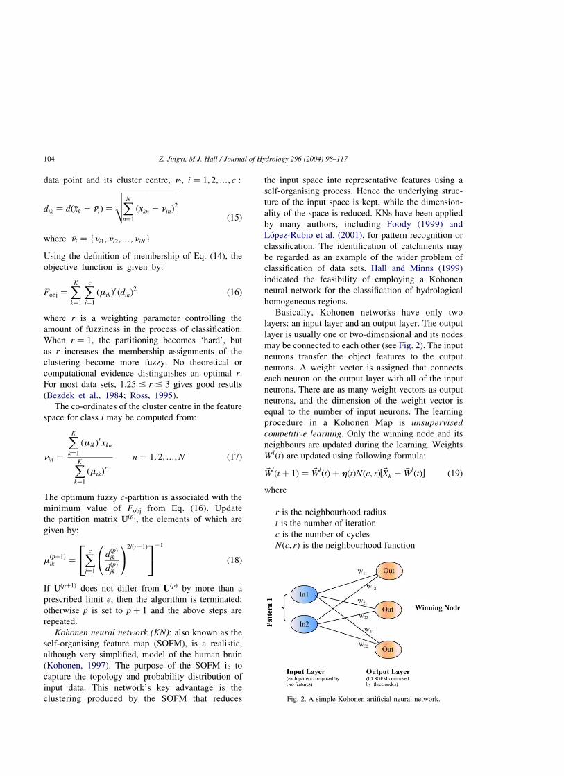
Basically, Kohonen networks have only two

layers: an input layer and an output layer. The output

layer is usually one or two-dimensional and its nodes

may be connected to each other (see Fig. 2). The input

neurons transfer the object features to the output

neurons. A weight vector is assigned that connects

each neuron on the output layer with all of the input

neurons. There are as many weight vectors as output

neurons, and the dimension of the weight vector is

equal to the number of input neurons. The learning

procedure in a Kohonen Map is unsupervised

competitive learning. Only the winning node and its

neighbours are updated during the learning. Weights

WlðtÞ are updated using following formula:

~Wlðt þ 1Þ ¼ ~WlðtÞ þ hðtÞNðc; rÞb~Xk 2 ~WlðtÞc ð19Þ

where

r is the neighbourhood radius

t is the number of iteration

c is the number of cycles

Nðc; rÞ is the neighbourhood function

Fig. 2. A simple Kohonen artificial neural network.


hðtÞ is the learning rate~Xk is the kth feature vector

The winning node is determined by a similarity

measure, which can be Euclidean distance measure

or the dot product of two vectors. The Euclidean

distance that is mostly used for similarity measure is

calculated as:

Dj ¼ kx 2 wk ¼

ffiffiffiffiffiffiffiffiffiffiffiffiffiffiffiffiffiXn

i¼1

ðxi 2 wjiÞ2

vuut ð20Þ

where

xi is the ith input signal;

wji is the weight of the connection from node i to

node j

Classification of the 86 catchments was carried out

using the NeuroSolutions software developed by

Neurodimensions Inc of Florida. Eight standardised

catchment characteristics were selected as input for

training the Kohonen neural network. The initial

learning rate was set to 0.45 and reduced by 0.0001

per epoch until it reached a final value of 0.001. Since

at least two or possibly three clusters were expected, a

set of 25 output nodes was adopted in the linear

SOFM. Four different neighbourhood radii ranging

from 9 to 12 were adopted to carry out the

simulations. Each simulation was repeated ten or

more times using different randomised weights for

each neighbourhood radius. The initial value of the

neighbourhood radius was reduced by 0.0025 per

epoch until it reached a final value of zero. The

principle of training a Kohonen neural network is the

same as that for any ANN, namely the repeated

presentation of the input data set until the output

response of each input vector has stabilised and the

resultant weight changes are negligible.

5. Application of classification methods

Four clustering methods, namely RM, WC, FC and

KN were applied to identify groupings of sites.

Wiltshire (1985) and Nathan and McMahon (1990)

among others have drawn attention to the large

amount of subjectivity involved in drawing

the regional boundaries by using RM. Different

hydrologists can obtain different groupings and the

geographical proximity is no guarantee of homogen-

eity since neighbouring catchments can be physically

different. To avoid geographical proximity, multi-

variate techniques (WC, FC and KN) which use

partitioning techniques can be applied. One of the

primary features of partitioning techniques is that the

allocation of a data point to a cluster is revocable, i.e.

although an object is assigned initially to a cluster, it

can be removed subsequently to other cluster.

The WC method manipulates the data points to

form the initial clusters and then uses the K-means

method to adjust inaccurately assigned sites. The FC

method assigns each data point to a particular class by

‘hardening’ the fuzzy partition matrix ðUÞ: For these

two methods, the expected number of classes must be

specified. However, the Kohonen network can both

select the number of clusters and allocate each site to a

cluster. Therefore, only the KN method as applied in

this study produces an objective estimate of the

number of clusters. Since the Kohonen network

indicated that a division into three sub-regions was

most appropriate, the results obtained from the other

methods are also presented for this number of clusters

or classes.

The classification results from applying the four

techniques are shown in Tables 1 and 2. In Table 1,

comparing RM with KN, only 38% of the sites are the

same, but for the other three methods the percentages

of the common sites were 90% and more. In

particular, the percentage of the common sites

reached 98% when comparing WC and FC. Class III

had the same 25 sites, and class I and class II only had

two different sites out of 39 sites and 24 sites,

respectively.

There is no clear difference between average

catchment characteristics of each class by using

RM, as shown in Table 2, but the results of the WC,

FC and KN methods display notable agreement. Fig. 3

shows the distribution of sites for the three classes

obtained by using KN. All sites belonging to class III

were located in the flat areas of Jiangxi province with

large catchment areas (AREA < 4000 km2), long

main stream lengths (MSL < 160 km), lower mean

catchment altitudes (MCA around 300 m), lower

geological feature indices (GFI < 0.55) and lower

plantation indices (PLANT < 0.15). Most sites of


class II are located in the hilly areas of Fujian

province with steep slopes (WMS < 50), larger

average annual rainfalls (AAR < 1760 mm), higher

MCA (<600 m) and higher PLANT (<0.60). The

class I sites are located in the mountainous boundary

between provinces, with shorter river lengths, higher

mean annual maximum catchment 1-day rainfalls and

higher GFI values. These results indicate that using

the WC, FC and KN methods with three classes

provided a consistent correlation with topography and

precipitation patterns.

When homogeneous regions have been at least

tentatively identified, the discordancy and homogen-

eity measures based on at-site L-moment statistics can

be calculated for a proposed region. If any site is

discordant with the region as a whole, the possibility of

moving that site to another region should be con-

sidered. Discordancy measures were calculated for

the original 86 sites and for the different groups formed

by applying the different classification methods. There

were 10 sites (Nos. 4, 31, 53, 54, 55, 60, 69, 70, 83 and

90) out of the 86 for which the Di value exceeds the

critical value ðDi $ 3Þ: The discordancy and hom-

ogeneity measures for all 3 classes are given in Table 3.

The locations of the 10 sites that were flagged as

discordant are also indicated in Fig. 3.

Table 3 shows that the sites 54, 83 and 90 were

always found to be discordant when using every

classification method, but the sites 4 and 31 were so

identified only when using the WC, FC and KN

methods. Site 55 was not identified as discordant in

any of the three classes for the WC, FC and KN

methods. The sites that were flagged as discordant

from the original groups were removed to form new

groups. A heterogeneity measure was computed for all

new groups, but there was no obvious improvement in

Table 1

Comparison between numbers of sites per sub-region identified by four different classification techniques, along with numbers common to one

or more methods

Three classes Method No. of common sites

RM WC FC KN RM/KN FC/KN WC/FC WC/KN WC/FC/KN

I 43 37 39 44 21 38 37 36 36

II 20 24 22 20 5 19 22 19 19

III 23 25 25 22 7 22 25 22 22

Total 86 86 86 86 33 79 84 77 77

Percentage (%) 38 92 98 90 90

RM, method of residuals; KN, Kohonen network; WC, Ward’s method; FC, fuzzy c-means method).

Table 2

Representative regional catchments (RRCs) for three sub-regions and four different classification techniques

Class Method AREA MSL WMS AAR APBAR MCA GFI PLANT

Three classes I RM 1578 86 22 1710 100 444 0.625 0.341

WC 747 60 15 1689 101 424 0.683 0.255

FC 731 59 17 1687 100 441 0.681 0.260

KN 882 67 17 1689 100 448 0.664 0.269

II RM 1735 103 27 1692 99 492 0.624 0.323

WC 815 79 50 1753 97 664 0.650 0.595

FC 850 82 51 1763 99 655 0.650 0.617

KN 685 76 51 1767 98 656 0.679 0.621

III RM 1937 97 13 1702 98 448 0.670 0.279

WC 3996 156 2 1678 98 306 0.556 0.153

FC 3996 156 2 1678 98 306 0.556 0.153

KN 4300 160 2 1674 98 292 0.543 0.150

RM, method of residuals; KN, Kohonen network; WC, Ward’s method; FC, fuzzy c-means method.


homogeneity. As Hosking and Wallis (1997) have

noted, a site’s L-moments may differ by chance alone

from those of other physically similar sites. For

example, an extreme but localised meteorological

event may have affected only a few sites in a region. If

such an event is approximately equally likely to affect

any of the sites in the future, then the entire group of

sites should be treated as a homogeneous region, even

though some sites may appear to be discordant with

the region as a whole. For this case study, whether

localised meteorological events have affected these 10

sites needed further investigation.

Fig. 3 shows that some sites (60, 69 and 70) are

located near the boundary between Fujian province

Fig. 3. Location of the sites belonging to the three classes as identified by the Kohonen SOFM; the 10 discordant sites are indicated by the

triangles.

Table 3

Numbers of discordant sites and homogeneity indices per sub-region for four different classification methods. The ‘new’ groups were obtained

by omitting the discordant sites.

Class Name of sites (discordancy $ 3) Homogeneity Homogeneity of new group

RM WC FC KN RM WC FC KN RM WC FC KN

I 83/90 83 83 54/90 20.22 1.75 1.67 1.54 1.00 2.06 1.79 1.92

II 54 90 90 83 0.45 1.11 1.08 0.93 2.71 1.08 1.17 1.45

III 55 4/31/54 4/31/54 4/31 3.63 20.54 20.54 20.12 0.02 21.26 21.26 21.16

Total 4 5 5 5



and Zhejiang province where rainfall is frequent in

spring, summer and autumn. The main rainfall pattern

of Zhejiang province is typhoon rain in summer. Sites

4, 31, 53, 54 and 55 are located in the mountainous

area in the southern part of Jiangxi province where the

precipitation is high in autumn. The typhoon rain also

affects this area. The position of sites 83 and 90 is near

the coast of the East Sea where typhoon rain is the

main rainfall pattern. According to the topography

and precipitation patterns and spatial distribution of

these locations, the possibility cannot be excluded that

localised meteorological events have affected these

sites. All these 10 sites were therefore kept in their

original groups. Class III for all three methods (WC,

FC, KN) and class II for the KN method were

acceptably homogeneous ðH , 1Þ: The H values of

other class are less than 2, so that these classes can

also be considered as defining a homogeneous region.

The principal conclusion to be drawn from this

comparison of methods for identifying sub-regions is

the similarity in the groupings of sites obtained using

the Kohonen network, Ward’s method and the Fuzzy

c-means method. Since all three approaches were

based on Euclidean distance as a similarity measure,

such a level of agreement could be anticipated.

However, of the three techniques, only the KN

method provides an objective number of sub-regions

as well as defining their membership, and as such is to

be preferred. However, the Fuzzy c-means method

provides for each site the membership levels associ-

ated with each class or sub-region. These fractional

memberships may then be employed as weights in

developing the at-site growth curve from those

applicable to each sub-region. A preliminary evalu-

ation of this approach is described in Section 6 below.

6. Determination of regional frequency

distributions

After successful use of the classification methods, a

probability distribution has to be chosen for fitting to

each region’s data. The goodness-of-fit measure based

on L-moments was used to test whether a selected

distribution is acceptable and to find the best-fitting

distribution. Table 4 showed the results of goodness-

of-fit analysis for the Gan-Ming river basin data and

indicated that the GEV, LN3 and PE3 distributions

give acceptably close fits to the regional average

L-moments. The choice of a suitable standard

frequency distribution is often controversial, but the

General Extreme Value (GEV) distribution has

obtained widespread acceptance (Hall and Minns,

1998). Therefore, the GEV distribution was selected

for fitting regional growth curves to Gan-Ming River

basin flood data.

Essentially, a regional estimation method is a

technique for transferring information from the sites

deemed to possess pertinent hydrological information

to the site at which a quantile estimate is needed.

Many regional estimation methods have been

suggested in the literature. Only the L-moments

method, the membership weights method and artifi-

cial neural networks were used in this study.

Regional L-moment algorithm: The index-flood

procedure uses summary statistics of the data at each

site and combines them by weighted averaging to

form the regional estimates. When the summary

statistics are the L-moment ratios of the at-site data,

the resulting procedure is called the regional

L-moment algorithm (Hosking and Wallis, 1997).

The regionalisation procedure is as follows:

† The flow data at each site i are arranged in

ascending order, i.e. q1 # q2 # · · · # qni: The

probability-weighted moments bri at each site i

are estimated using equation:

bri ¼n21i

Xni

j¼rþ1

ðj 2 1Þðj 2 2Þ· · ·ðj 2 rÞ

ðni 2 1Þðni 2 2Þ· · ·ðni 2 rÞqj:ni

;

r ¼ 0; 1; 2… ð21Þ

where qj is the jth smallest in the ordered sample of

events, and ni is the sample size of site i:

† The at-site sample L-moments lri and the

sample L-moment ratios tr are estimated using

equation:

lr ¼ n21i

Xni

j¼1

wðrÞj:ni

qj:nið22Þ

tr ¼ lr=l2

and the sample L 2 CV is:

t ¼ l2=l1 ð23Þ


Here the weights wðrÞj:n are the discrete Legendre

polynomials (Hosking and Wallis, 1997):

wðrÞj:ni

¼ ð21Þr21Pr21ðj 2 1; ni 2 1Þ ð24Þ

† The regional L-moments estimators are then

calculated using weights proportional to the

sites’ record length:

tR ¼XNi¼1

nitðiÞ

�XNi¼1

ni; ð25Þ

tRr ¼

XNi¼1

nitðiÞr

�XNi¼1

ni; r ¼ 3; 4;…

where N is the number of stations. The regional

average mean is set to 1, that is, lR1 ¼ 1:

† The parameters of the regional frequency

distribution are estimated using the estimators

of regional L-moments.

† For each site, the at-site quantile is obtained by

multiplying the at-site mean with the corre-

sponding dimensionless regional flow quantile,

qr: The estimate of quantile with non-excee-

dance probability F is:

QiðFÞ ¼ lðiÞ1 qT ðFÞ ð26Þ

The regional L-moment algorithm was applied to

the Gan-Ming River basin using a FORTRAN

program developed by Hosking (2000). The

regional average L-moments ratio and estimated

regional parameters for GEV distributions fitted to

the regions are indicated in Table 5. The regional

frequency growth curve can be expressed as

follows for the different regions:

qðFÞ ¼jþ a{1 2 ð2log FÞk}=k; k – 0

j2 a logð2log FÞ; k ¼ 0

(ð27Þ

Here j (location), a (scale) and k (shape) are

regional parameters of GEV distribution.

Fuzzy Membership Weights method: A site may be

regarded as not belonging totally to a particular region

but as having fractional membership in several

regions. As described by Hall and Minns (1999), in

fuzzy classification, the fuzzy partitions are ‘soft’, i.e.

each point is allowed a degree of membership in more

than one class. Then each data point can be assigned

to the class by hardening the fuzzy partition matrix.

The largest element in each column of the matrix is set

to unity and all the other elements are set to zero.

However, parameters or quantiles for the site can be

estimated by a weighted average of the corresponding

estimates for different regions using the degrees

of membership as weights. Similar weighting

Table 4

Goodness-of-fit analysis for five different frequency distributions when applied to the three groupings of sites identified by four classification

techniques

Methods Member Z-test

GLO GEV LN3 PE3 GPA

86 sites 5.04 0.89 20.22 22.45 28.71

Residual method (three classes) RM-1 43 sites 1.75 0.12 20.47 21.58 23.78

RM-2 20 sites 2.67 0.44 20.01 21.01 24.60

RM-3 23 sites 3.75 0.78 0.00 21.57 26.06

Ward’s cluster method (three classes) WC3-1 37 sites 3.59 0.99 0.23 21.27 25.08

WC3-2 24 sites 1.86 20.03 20.55 21.59 24.41

WC3-3 25 sites 2.75 0.34 20.21 21.37 25.17

Fuzzy c-means (three classes) FC3-1 39 sites 3.68 0.98 0.18 21.39 25.33

FC3-2 22 sites 1.84 20.03 20.52 21.52 24.34

FC3-3 25 sites 2.75 0.34 20.21 21.37 25.17

Kohonen network KN-1 44 sites 3.76 0.93 0.17 21.36 25.61

KN-2 20 sites 1.40 20.25 20.82 21.90 24.19

KN-3 22 sites 2.91 0.54 0.03 21.06 24.85

GLO, generalised Logistic; GEV, general extreme value; LN3, 3-parameter lognormal; PE3, Pearson type III; GPA, generalised Pareto.


approaches have been proposed, for example, by

Wiltshire (1986) and Acreman and Sinclair (1986).

Such weighting methods can equally well be used for

estimation of distribution parameters such as t or t3

and for estimation at ungauged sites.

In this study, class FC3 (25 sites) is selected as an

example. The membership levels are ai; bi and ci for

site i; respectively. The at-site mean is lðiÞ1 ; and the

regional growth curve is qjðFÞ for group j: Table 6

summarises the fuzzy memberships and root mean

square error (RMSE) between observed data and

computed quantiles. The latter were estimated using

the at-site mean and the three regional growth curves,

all derived using the L-moment method. Quantiles

were estimated by using the weighted average of the

corresponding estimates for the different regions with

the at-site membership levels as the weights. The

RMSEs of most sites obtained by using the at-site

estimated quantiles were smaller than those obtained

by using either the specific regional growth curve for

the sites or the weighted regional estimates. The

RMSEs for weighted estimates were close to those for

the regional growth curve. The estimated quantiles of

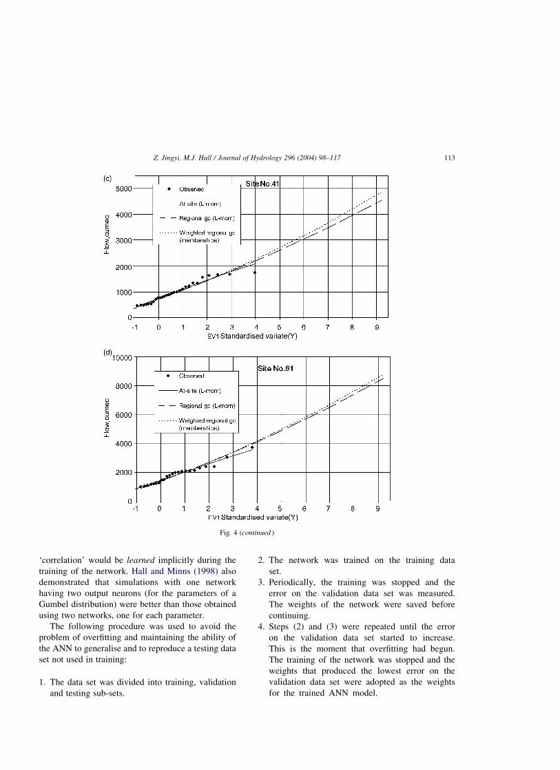
sites 7, 26, 41 and 61 are compared in Fig. 4. This

figure indicates that the average weighted quantiles of

site 7 describe the observed floods better, while sites

26, 41 and 61 were found to either over-estimate or

under-estimate the quantiles using the specific

regional growth curve.

Similar somewhat inconclusive results were also

obtained for the other two sub-regions defined by

classes FC1 and FC2. The use of the membership

levels as weighting factors in forming a regional

estimate is likely to be more successful with data sets

in which the growth curves of the sub-regions display

a greater variety in shape than those in the Gan-Ming

river basin.

MLP Neural Network: A multilayer, feed-forward

perceptron-type network (MLP) is one of the most

commonly used types of neural network. A typical

three-layer feed-forward network, which has an input

layer, a hidden layer and an output layer, is shown in

Fig. 5. The processing elements in each layer are

called nodes or units. The numbers of nodes in the

input layer and the output layer are determined by the

dimensions of the input pattern and of the desired

outputs, respectively. Each of the nodes is fully

connected to all the nodes of the neighbouring layers.

The parameters associated each of these connections

are called weights. All connections are feed forward,

i.e. they allow information transfer only from an

earlier layer to the next consecutive layer. Nodes

within a layer are not interconnected, and nodes in

non-adjacent layers are not connected.

Table 5

The regional average L-moments ratios and the estimated regional parameters for GEV distributions fitted to three regions as determined by four

different classification algorithms

Methods Member Regional average L-moments ratio Regional estimators of the GEV

parameters

t t3 t4 t5 j a k

86 sites 0.2689 0.2090 0.1561 0.0647 0.7658 0.3660 20.0599

RM-1 43 sites 0.2774 0.2299 0.1687 0.0846 0.7532 0.3652 20.0912

RM-2 20 sites 0.2661 0.1938 0.1505 0.0535 0.7721 0.3706 20.0368

RM-3 23 sites 0.2666 0.2089 0.1539 0.0614 0.7678 0.3629 20.0597

WC3-1 37 sites 0.2801 0.2150 0.1527 0.0627 0.7545 0.3776 20.0690

WC3-2 24 sites 0.2682 0.2111 0.1639 0.0633 0.7659 0.3638 20.0630

WC3-3 25 sites 0.2547 0.1995 0.1548 0.0684 0.7804 0.3517 20.0455

FC3-1 39 sites 0.2813 0.2161 0.1538 0.0629 0.7532 0.3786 20.0706

FC3-2 22 sites 0.2645 0.2085 0.1628 0.0629 0.7698 0.3602 20.0592

FC3-3 25 sites 0.2547 0.1995 0.1548 0.0684 0.7804 0.3517 20.0455

KN-1 44 sites 0.2780 0.2095 0.1523 0.0655 0.7578 0.3780 20.0606

KN-2 20 sites 0.2675 0.2261 0.1742 0.0645 0.7629 0.3543 20.0855

KN-3 22 sites 0.2540 0.1959 0.1500 0.0635 0.7819 0.3526 20.0401



Each node j receives incoming signals from every

node i in the previous layer. Associated with each

incoming signal xi; there is a weight wji: The effective

incoming signal Sj to node j is the weighted sum of all

the incoming signals and Sj passes through a non-

linear activation function (sometimes called a transfer

function or threshold function) to produce the out-

going signal yj of the node.

The output from the output node is compared with

the target output and the error is propagated back to

adjust the connecting weights. This procedure is

called backpropagation. The weight associated with

each connection is adjusted by an amount pro-

portional to the strength of the signal in the connection

and total measure of the error (see Rumelhart et al.,

1994). This process is repeated many times with many

different input/output tuples until a sufficient accuracy

for the data set has been obtained.

In this study, an ANN was employed in order to

develop a relationship between the parameters of

the regional flood frequency distribution for each site

and the characteristic features of the upstream

catchment. The performance of the ANN could then

be compared to that of the regional expression of

Eq. (13) obtained by linear regression analysis. The

properties of an ANN as a universal approximator

(Hornik et al., 1989) are such that the information

contained in the training data is encapsulated in a

reduced number of weights unconstrained by assump-

tions of linearity in the relationship between depen-

dent and independent variables or their transforms.

Unfortunately, in training an MLP, the number of

weights in the network should be about one-quarter or

less than the number of training data (see, e.g.

Walczak and Cerpa, 1999) in order not to impair the

ability of the ANN to generalise. Using the same

catchment features as those used in the regression

analysis, each ANN would have five inputs and one

output. Allowing for at least two nodes in the hidden

layer, the total number of weights would be 12,

Table 6

The fuzzy membership levels (a,b,c) and RMSEs for 25 sites in class FC3

No. Name L-mean Membership value RMSE

a b c At-site Regional gc Weighted regional gc

4 Nindu 1141 0.742 0.192 0.066 101 150 148

5 Fengkeng 2527 0.919 0.052 0.029 159 150 152

7 Hanlinqiao 1373 0.805 0.137 0.059 122 123 124

8 Fengkengkou 1665 0.884 0.078 0.038 226 249 245

9 Julongtan 2186 0.843 0.092 0.065 175 203 204

12 Yaoxiaba 675 0.773 0.181 0.047 47 70 75

13 Bashang 1826 0.920 0.050 0.030 131 182 179

22 Duotou 1218 0.706 0.211 0.083 102 123 129

23 Shangshalan 1910 0.871 0.083 0.045 145 134 135

25 Saitang 1324 0.743 0.177 0.08 61 65 66

26 Xintian 1728 0.963 0.027 0.011 128 126 125

31 Maozhou 1581 0.714 0.211 0.075 62 284 302

32 Jiacun 2072 0.937 0.042 0.022 129 289 294

34 Niutoushan 1428 0.932 0.051 0.017 116 156 153

38 Diaoshui 2020 0.941 0.041 0.017 146 149 150

40 Loujiacun 2089 0.919 0.054 0.026 134 240 245

41 Taopo 946 0.570 0.358 0.072 85 106 113

45 Dufengkeng 3410 0.745 0.169 0.086 152 423 453

49 Xiangtun 3270 0.623 0.246 0.131 226 249 277

50 Hushan 4456 0.872 0.084 0.045 203 297 315

51 Gaosha 3855 0.886 0.081 0.033 376 608 597

54 Xianfeng 1366 0.675 0.271 0.054 263 435 424

56 Wanjiabu 2114 0.643 0.244 0.113 193 267 245

58 Shangrao 2433 0.762 0.172 0.066 200 259 276

61 Pashi 1772 0.783 0.151 0.066 117 163 174


requiring at least 50 data tuples for training. However,

Table 1 indicates that none of the identified sub-

regions had this number of members. Therefore, the

comparison was carried out on the pooled data set of

86 sites for demonstration purposes.

The five catchment characteristics used in devel-

oping Eq. (13) were employed as inputs and the three

parameters ðj;a; kÞ of the GEV distribution fitted to

the annual floods recorded at each gauged site were

employed as outputs. Initially, a choice had to be

made regarding the suitability of applying a single

ANN with three outputs or of training separately three

ANNs with a single output for j;a and k; respectively.

An ANN with only one output neuron would, of

course, contain fewer weights than an ANN with three

output neurons, giving rise to a simple network that

would be correspondingly faster and easier to train.

However, the j;a and k parameters forming the

outputs are not entirely independent, as can be seen

from the form of Eqs. (27). Use of three separate

ANNs would therefore ignore this connection, but by

combining the outputs in a single ANN this

Fig. 4. Plots of the GEV distribution fitted to flood samples using the membership weights method for four stations: (a) site no. 7; (b) site no. 26;

(c) site no. 41; (d) site no. 61.


‘correlation’ would be learned implicitly during the

training of the network. Hall and Minns (1998) also

demonstrated that simulations with one network

having two output neurons (for the parameters of a

Gumbel distribution) were better than those obtained

using two networks, one for each parameter.

The following procedure was used to avoid the

problem of overfitting and maintaining the ability of

the ANN to generalise and to reproduce a testing data

set not used in training:

1. The data set was divided into training, validation

and testing sub-sets.

2. The network was trained on the training data

set.

3. Periodically, the training was stopped and the

error on the validation data set was measured.

The weights of the network were saved before

continuing.

4. Steps (2) and (3) were repeated until the error

on the validation data set started to increase.

This is the moment that overfitting had begun.

The training of the network was stopped and the

weights that produced the lowest error on the

validation data set were adopted as the weights

for the trained ANN model.

Fig. 4 (continued )


The data set was divided into a training set of

55 catchments, a cross-validation set of 15 catch-

ments and a test set of 16 catchments. The 16

catchments for the testing set were chosen such

that the values of variables were within the range

of variable values of the training data set. One

hidden layer with the sigmoidal activation function

was used to set up the network. The number of

nodes in the hidden layer was varied from two to

five (12–28 weights), with each run being repeated

with several different initial weight values in order

to identify a ‘best’ network.

Figs. 6–8 present the results of testing the ANN,

and show that the MLP network was unable to capture

entirely the variations in the parameter k: The

performance of this ANN for the GEV parameters

was compared with the mean annual flood plus growth

curve approach. Two flood magnitudes were selected:

the mean annual flood, MAF and the 50-year flood.

Scatter plots of the regression MAF from Eq. (13) and

the ANN MAF computed from Eq. (26) against the

‘observed’ MAF are shown in Fig. 9. In addition to the

scatter plot, the root mean square errors between

the computed and observed values were calculated.

Fig. 5. A typical three-layer MLP neural network.

Fig. 6. Scatter plots of observed versus simulated location

parameters for both training and testing data using an MLP network.

Fig. 7. Scatter plots of observed versus simulated scale parameters

for training data and testing data using an MLP network.


The values obtained were 380 m3/s for the regression

equation and 314 m3/s for the ANN, an improvement

of some 18% of the latter over the former.

The above exercise was repeated for the 50-year

flood. In the case of the ANN model, Eq. (26) gives

the required quantile directly. For the regression

model, the MAF from Eq. (13) must be multiplied by

the appropriate growth factor, which from Eq. (27)

and Table 5 was 2.375 for the 86 sites. The ‘observed’

50-year flood may also be estimated using Eq. (26),

but using j;a and k obtained from the recorded annual

floods. The root mean square errors were 903 m3/s for

the regression equation and 665 m3/s for the ANN, an

improvement of some 26% of the latter over the

former. The scatter plot shown in Fig. 10 is similar to

Fig. 9, demonstrating that, in general, the ANN model

was capable of providing better estimates of the MAF

than the regression model.

7. Conclusions and recommendations

To date, flood frequency analysis in the Gan-Ming

River basin has mainly focused on at-site analysis

using the Pearson Type 3 distribution. However, in

this study, a regional approach has been taken in

which the gauging sites were first classified into

groups using catchment and rainfall characteristics,

and then the at-site flow records were employed to

evaluate the discordancy and the homogeneity of the

groups. The classification methods employed

included the residuals method, a widely used cluster-

ing algorithm, a fuzzy classification method and a

Kohonen artificial neural network. Substantial agree-

ment on the groupings of sites was achieved using the

clustering technique, the fuzzy classification method

Fig. 8. Scatter plots of observed versus simulated shape parameter

for training data and testing data using MLP network.

Fig. 9. Scatter plots of computed versus observed mean annual

floods for 86 sites.

Fig. 10. Scatter plots of computed versus observed 50-year floods

for 86 sites.


and the Kohonen network, Such agreement was to be

expected since all three approaches are based upon the

use of Euclidean distance as a similarity measure.

However, as implemented in this study, Ward’s

method and the fuzzy c-means methods required the

number of classes to be set by the analyst (although a

tournament selection algorithm is now available for

the fuzzy classification method; see Endo and

Yamaguchi, 1998). The Kohonen SOFM, which

provides an estimate of the number of classes as

well as identifying the class membership, was there-

fore the preferred approach. No attempt was made at

classifier fusion, i.e. the combination of the results

obtained by application of the different techniques to

achieve a consensus, or classifier selection, i.e. the

identification of regions in the feature space where

one approach is the most ‘expert’ (see, e.g. Liu and

Yuan, 2001).

The use of a clustering algorithm on catchment

characteristics, followed by the examination of the

discordancy and homogeneity of the identified groups

based on at-site L-moments of the distribution of

annual floods, revealed that a small number of sites in

the Gan-Ming river basin appeared to be discordant.

However, further investigation showed that, since all

the apparently discordant sites were subject to the

influence of typhoon rains, there was no basis for

excluding them from the regional analysis. This result

may also be interpreted as an indication that a new

variable, reflecting the influence of such heavy and

infrequent precipitation, should be added to the list of

catchment and rainfall characteristics and the classi-

fication exercise repeated in order to refine the initial

groupings of sites reported here.

In addition to the use of a Kohonen SOFM as a

classifier, ANNs were also used to relate the

parameters of the at-site flood frequency distri-

butions to catchment and rainfall characteristics.

Since only 86 sites were available, the size of the

classes was insufficient to train and test MLP

networks for each sub-region. However, a compari-

son between the regional regression equation

obtained by MLRA and an MLP using the data

from all sites was sufficient to demonstrate the

advantages of ANNs as universal approximators

over linear regression in reducing the standard

errors of estimate of the predicted flood quantiles.

The improvement in standard errors was obtained

despite the poorer performance of the ANN in

capturing the variations of the shape parameter of

the GEV distribution compared with that for the

scale and location parameters. Further investigation

of the ANN approach using larger regional data

sets is therefore recommended.

The use of the membership levels obtained by the

application of the Fuzzy c-means algorithm as

weights in the determination of the at-site growth

curves proved to be inconclusive in this study, partly

because of the relatively small differences in the

growth curves of the identified regions (see Table 5).

However, the further evaluation of this technique is

recommended.

References

Acreman, M.C., Sinclair, C.D., 1986. Classification of drainage

basins according to their physical characteristics: an appli-

cation for food frequency analysis in Scotland. J. Hydrol. 84,

365–380.

Bezdek, J.C., Ehrlich, R., Full, W., 1984. FCM: the fuzzy c-means

clustering algorithm. Comput. Geosci. 10(2–3), 191–203.

Cunnane, C., 1988. Methods and merits of regional flood frequency

analysis. J. Hydrol. 100, 269–290.

Endo, Y., Yamaguchi, S., 1998. Tournament fuzzy clustering

algorithm with automatic cluster number estimation. Electron.

Commun. Jpn Part 3 81(2), 46–58.

Foody, G.M., 1999. Applications of the self-organising feature map

neural network in community data analysis. Ecol. Modell. 120,

97–107.

French, M.N., Krajewski, W.F., Cuykendall, R.R., 1992. Rainfall

forecasting in space and time using neural network. J. Hydrol.

137, 1–31.

Greenwood, J.A., Landwehr, J.M., Matalas, N.C., Wallis, J.R.,

1979. Probability weighted moments: definition and relation to

parameters of several distributions expressable in inverse form.

Water Resour. Res. 15, 1049–1054.

Groupe de recherche en hydrologie statistique (GREHYS), 1996.

Presentation and review of some methods for regional flood

frequency analysis. J. Hydrol. 186, 63–84.

Hall, M.J., Minns, A.W., 1998. Regional flood frequency analysis

using artificial neural network. In: Babovic, V., Larsen, L.C.

(Eds.), Proceedings of the Third International Conference on

Hydroinformatics (Copenhagen, Denmark), vol. 2. Balkema,

Rotterdam, pp. 759–763.

Hall, M.J., Minns, A.W., 1999. The classification of hydrological

homogeneous regions. J. Hydrol. Sci. 44(5), 693–704.

Hall, M.J., Minns, A.W., Ashrafuzzaman, A.K.M., 2002. The

application of data mining techniques for the regionalisation

of hydrological variables. Hydrol. Earth Syst. Sci. 6(4),

685–694.


Hornik, K., Stinchcombe, M., White, H., 1989. Multilayer

feedforward networks are universal approximators. Neural

Networks 2, 359–366.

Hosking, J.R.M. 2000. Fortran routines for use with the method of

L-moments, Version 3.03, (http://lib.stat.cmu.edu/general/lmo-

ments).

Hosking, J.R.M., Wallis, J.R., 1997. Regional Frequency Analysis:

An Approach Based on L-moments, Cambridge University

Press, Cambridge, ISBN 0-521-43045-3.

Kohonen, T., 1997. Self-Organizing Maps, 2nd ed., Springer,

Berlin, ISBN 3-540-62017-6.

Liu, R., Yuan, B., 2001. Multiple classifiers combination by

clustering and selection. Information Fusion 2, 163–168.

Lopez-Rubio, E., Munoz-Perez, J., Gomez-Ruiz, J.A., 2001.

Invariant pattern identification by self-organising networks.

Pattern Recogn. Lett. 22, 983–990.

Minns, A.W., Hall, M.J., 1996. Artificial neural networks as

rainfall-runoff models. Hydrol. Sci. J. 41(3), 399–417.

Muttiah, R.S., Srinivasan, R., Allen, P.M., 1997. Prediction of two-

year peak stream discharges using neural networks. J. Am.

Water Resour. Assoc. 33, 625–630.

Nathan, R.J., McMahon, T.A., 1990. Identification of homogeneous

regions for the purpose of regionalisation. J. Hydrol. 121,

217–238.

Robson, A.J., Reed, D.W., 1999. Flood Estimation Handbook, vol.

3. Institute of Hydrology, Wallingford.

Ross, T.J., 1995. Fuzzy Logic with Engineering Aplications,

McGraw-Hill, New York, ISBN 0-07-053917-0.

Rumelhart, D.E., Widrow, B., Lehr, M.A., 1994. The basic ideas in

neural networks. Commun. ACM 37(3), 87–92.

Vogel, R.M., Fennessey, N.M., 1993. L-moment diagrams should

replace product moment diagrams. Water Resour. Res. 29(6),

1745–1752.

Walczak, S., Cerpa, N., 1999. Heuristic principles for the design of

artificial neural networks. Information Software Technol 41,

109–119.

Ward, J.H., 1963. Hierarchical grouping to optimize an objective

function. J. Am. Stat. Assoc. 58, 236–244.

Wiltshire, S.E., 1985. Grouping of catchments for regional food

frequency analysis. Hydrol. Sci. J. 30, 151–159.

Wiltshire, S.E., 1986. Regional food frequency analysis: Hom-

ogeneity statistics. Hydrol. Sci. J. 31, 321–333.


http://lib.stat.cmu.edu/general/lmoments

http://lib.stat.cmu.edu/general/lmoments

Regional flood frequency analysis for the Gan-Ming River basin in China

Documents

Transcript of Regional flood frequency analysis for the Gan-Ming River basin in China