No. 07-E-22 November 2007

REGIME SWITCHES IN EXCHANGE RATE VOLATILITY AND UNCOVERED INTEREST PARITY Hibiki Ichiue* hibiki.ichiue@boj.or.jp Kentaro Koyama ** kentarou.koyama@boj.or.jp Bank of Japan 2-1-1 Nihonbashi Hongoku-cho, Chuo-ku, Tokyo 103-8660

* Research and Statistics Department ** Financial Markets Department Papers in the Bank of Japan Working Paper Series are circulated in order to stimulate discussion and comments. Views expressed are those of authors and do not necessarily reflect those of the Bank. If you have any comment or question on the working paper series, please contact each author. When making a copy or reproduction of the content for commercial purposes, please contact the Public Relations Department (webmaster@info.boj.or.jp) at the Bank in advance to request permission. When making a copy or reproduction, the source, Bank of Japan Working Paper Series, should explicitly be credited.

Bank of Japan Working Paper Series

1

REGIME SWITCHES IN EXCHANGE RATE VOLATILITY AND

UNCOVERED INTEREST PARITY#

Hibiki Ichiue♦ and Kentaro Koyama∗

November 2007

Abstract

We use a regime-switching model to examine how exchange rate volatilities

influence the failure of uncovered interest parity (UIP). Main findings are as follows.

First, exchange rate returns are significantly influenced by regime switches in the

relationship between the returns and interest rate differentials. Second, appreciation of

low-yielding currencies occurs less frequently but is faster than the depreciation. Third,

low volatilities and UIP failure are mutually dependent. Finally, these findings are more

evident for three-month maturity than six-month maturity. These results are consistent

with market participants’ views: the short-term carry trade in a low-volatility

environment and its rapid unwinding substantially influence exchange rates.

Keywords: Uncovered interest rate parity, Forward discount puzzle, Carry trade,

Markov-switching model, Bayesian Gibbs sampling

# We would like to thank Naohiko Baba, James D. Hamilton, Keiji Kono, Mototsugu Shintani, Toshiaki Watanabe, Tomoyoshi Yabu, and the staff at the Bank of Japan for their helpful comments. The views expressed here are solely ours, and do not necessarily reflect those of the Bank of Japan. ♦ Senior Economist and Director, Research and Statistics Department, Bank of Japan; e-mail: hibiki.ichiue@boj.or.jp ∗ Economist, Financial Markets Department, Bank of Japan; e-mail: kentarou.koyama@boj.or.jp

2

1. Introduction

Lower-interest-rate currencies tend to depreciate relative to higher-interest-rate

currencies. This observation is inconsistent with one of the most popular theories,

uncovered interest parity (UIP), but has been confirmed for many currencies and periods

in the extensive literature on the subject. Even though more than 20 years have passed

since Fama (1984) called this inconsistency the “forward discount puzzle,” the failure of

UIP is still one of the most prominent puzzles in economics. In fact, there is no

consensus on how to explain the puzzle yet, and researchers still continue to tackle the

problem.1

In contrast, many market participants including monetary authorities seem to

have reached the consensus that the depreciation of lower-interest currencies has been

influenced by the carry trade activities in a low-volatility environment. A simple

definition of the carry trade is “borrowing in a low-interest currency to invest in a higher

one to earn the interest differential (the ‘carry’)”. For instance, de Rato (2006), Managing

Director of the IMF, mentioned that the carry trade reflects low volatilities and large

interest rate differentials, which lead to high Sharpe ratios of such trade, and has exerted

downward pressure on one of the lowest-interest currencies, the Japanese yen. He also

warned that the unwinding of the carry trade positions could lead to rapid reversal

movements of exchange rates.2

1 See Chinn and Meredith (2004), Alvarez, Atkeson and Kehoe (2005), Burnside, Eichenbaum,

Kleshchelski and Rebelo (2006), Plantin and Shin (2006), and Lustig and Verdelhan (2007), for instance.

2 de Rato said, in his speech: “As a result, despite a large current account surplus, there has been downward pressure on the yen in the short run. Indeed, in real effective terms, the yen is now at a 20-year low.” “The carry trade is not a consequence of global imbalances. Rather, it reflects the

3

In this paper, we employ a regime-switching model to investigate what role

exchange rate volatilities play in the failure of UIP. The idea to use regime-switching

models in examining exchange rates is not new. After Hamilton (1989) proposed the

regime-switching model to examine the persistency of recessions and booms, many

papers, including Engel and Hamilton (1990), Bekaert and Hodrick (1993), Engel (1994),

Bollen, Gray and Whaley (2000), and Dewachter (2001), applied this model to exchange

rate data. We extend these models to closely investigate the relationship among exchange

rate returns, volatilities, and interest rate differentials.

In estimating the model, we employ a Bayesian Gibbs sampling. Our method is

an extension of those used in the literature, such as Albert and Chib (1993), Kim, Nelson

and Startz (1998), and Kim and Nelson (1999). There is a new aspect in our method,

however. With this estimation method, we can examine higher-frequency state

transmissions and, at the same time, avoid possible estimation biases arising from the use

of high-frequency data.

The empirical results basically support the market participants’ views: low

volatilities have influenced UIP failure. The reverse is also true. That is, we find that UIP

failure contributes to maintaining low volatilities as well. These results imply that UIP

failure and a low-volatility environment are mutually dependent. We also find that

low-interest-rate currencies appreciate less frequently, but once it occurs, its movement is

faster than when they depreciate. This may suggest that exchange rate movement is faster

when carry trade is unwound on a large scale, as mentioned by Breedon (2001) and globalization of financial markets and the current environment of low volatility and wide interest rate differentials.” “Moreover, both financial markets and countries are exposed to risks if there is a sudden reversal of financial flows. For example, a disruptive unwinding of carry trade positions occurred in October 1998, when the U.S. dollar fell by 15 percent against the Japanese yen in four days.”

4

Plantin and Shin (2006). All these results are more evident for shorter maturities, and this

suggests that UIP failure is influenced by short-term carry-trade activities.

The rest of this paper is organized as follows. Section 2 uses OLS regressions to

overview the basic empirical facts. Section 3 describes our regime-switching model, and

the estimated results are discussed in Section 4. Section 5 concludes this paper.

2. OLS Analysis

This section uses OLS regressions to overview the basic empirical facts. We first

replicate a traditional regression to test UIP with our updated data. UIP is defined as an

equation:

*, ,( ) ( ) /12t t n t t n t nE y y r r n+ − = − ⋅ , (1)

where ty denotes the log exchange rate of the home currency against the foreign

currency. The n -month interest rates in the home and foreign countries, ,t nr and *,t nr ,

are measured in rates per annum. The right-hand side of (1) is interpreted as the earnings

from the interest rate differential or the carry when investors borrow in the foreign

currency to invest in the home currency for n months. Thus this equation means an

arbitrage relationship in which the expected exchange rate return, ( )t t n nE y y+ − , cancels

out the earnings from the interest rate differential. Therefore, according to this theory, if

the foreign interest rate is lower than the home interest rate, the foreign currency should

5

appreciate on average.

A typical test of UIP is conducted using a regression of the form:

*, ,( ) 12 / ( )t n t t n t n t ny y n r rα β ε+ +− ⋅ = + − + , (2)

with a null hypothesis of 0α = and 1β = . We use the U.S. dollar (USD) as the home

currency, and the Japanese yen (JPY), British pound (GBP), Swiss franc (CHF), and

Deutsche mark (DEM) as the foreign currency. The data of exchange rates and interest

rates (three and six-month LIBOR) are obtained from the IMF International Financial

Statistics. We obtained end-of-month data over the period from January 1980 to April

2000 for DEM, since it was replaced by the Euro, and to May 2007 for the other

currencies. We use non-overlapping quarterly and semiannual data for our OLS analysis

with three and six-month interest rates, respectively, to avoid possible estimation biases

in standard errors arising from overlapping data.3

Table 1 reports the regression results. There are two noteworthy points. First,

all estimated slope coefficients, β ’s, are negative, and in seven cases of eight they are

significantly different from one at the five-percent-significance level. This result suggests

that lower-interest currencies tend to depreciate, and is in opposition to what is predicted

by UIP. In particular, the slope coefficients for JPY are the largest in absolute values, and

are negative at the one-percent-significance level. The yen is thus the most puzzling

currency. Second, the point estimates of slope coefficients are closer to zero for longer

maturities, except for DEM; this is consistent with the findings of Alexius (2001) and 3 Using monthly overlapping data with heteroskedasticity and autocorrelation consistent standard errors, however, does not change the implications.

6

Chinn and Meredith (2004).

As reviewed in the preceding section, many market participants consider that a

low-volatility environment is an important factor in the recent carry trade activities,

which support the puzzling relationship, the depreciation of lower-interest currencies. To

confirm these views, we add another term to the traditional regression (2):

*0 , ,( ) 12 / ( )( )t n t v t t n t n t ny y n v r rα β β ε+ +− ⋅ = + + − + , (3)

where tv is the annualized historical volatility calculated using daily exchange rate

returns for 20 business days up to end-of-month. 0 v tvβ β+ in (3), as well as β in (2),

reflects the extent to which currency returns are related to interest rate differentials. Thus

a positive vβ means that a lower volatility leads to a lower 0 v tvβ β+ , i.e. a higher

deviation from what is predicted by UIP.

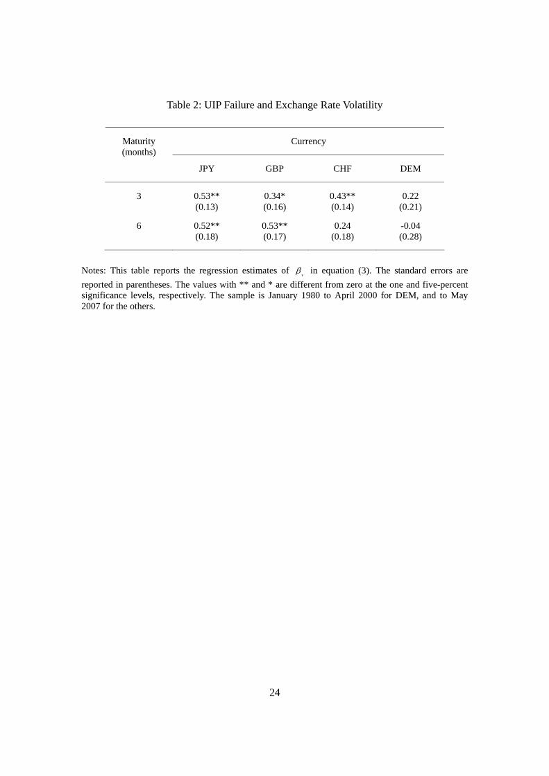
Table 2 shows that the point estimates of vβ are positive in seven cases out of

eight, and five of them are significantly different from zero at the five-percent

significance level. Thus, the puzzling relationship is stronger when the volatility is lower.

In particular, this tendency is most evident for JPY. That is, vβ of JPY is the largest for

three-month maturities, and is just slightly smaller than the largest, that of GBP, for

six-month maturities. In addition, only for JPY, both vβ ’s are positive at the

one-percent-significance level. These results do not seem to be just a coincidence with

the result seen in Table 1: JPY really is the most puzzling currency. On the contrary, these

results suggest that exchange rate volatilities play some role in the puzzling relationship.

7

Although we obtain some evidence for the relationship between UIP failure and

exchange rate volatility, the OLS analysis conducted here cannot help us understand their

causality. We will consider this issue using a regime-switching model, discussed in the

next section.

3. The Regime-Switching Model

The OLS analysis in the preceding section showed that the forward discount

puzzle is more evident for shorter maturities and under a lower-volatility regime. To

closely investigate these findings, we employ a regime-switching model. This section

discusses the model, and the empirical results are shown in the next section. Subsection

3.1 illustrates the idea of our model in comparison with models in the literature.

Subsection 3.2 defines the model in detail. Subsection 3.3 describes our estimation

strategy.

3.1. Comparison with the Models in the Literature

After Hamilton (1989) proposed the regime-switching model to examine the

persistency of recessions and booms, many papers have applied this model to exchange

rate data. In Engel and Hamilton’s (1990) two-regime model, currency returns are

specified as

1 1t t i i ty y α σ η+ +− = + , (4)

8

where {1,2}i∈ denotes the regime, iα and iσ denote the trend of exchange rate and

the volatility of exchange rate return under regime i , respectively, and 1 ~ (0,1)t Nη +

i.i.d. Engel and Hamilton estimate this model, and find that exchange rates have long

swings: exchange rates move in one direction for long periods of time. Engel (1994)

applies the same model to a large variety of currencies.

Bekaert and Hodrick (1993) also employ a two-regime model. They, however,

add an interest rate differential and a lag of exchange rate return in the model:

*1 1 1( ) ( )t t i i t t i t t i ty y r r y yα β γ σ η+ − +− = + − + − + , (5)

where tr and *tr denote one-period interest rates in the home and foreign countries.

Here the interest rates are measured in rates per period, rather than rates per annum, just

for notational convenience.4 Note that this two-regime model assumes simultaneous

switches in the intercept iα , the slope coefficient iβ , and the volatility parameter iσ .

The assumption of simultaneous switches in this model, as well as in the models of Engel

and Hamilton (1990) and Engel (1994), may be too restrictive; we will discuss this issue

later.

Bollen, Gray and Whaley (2000) and Dewachter (2004) employ four-regime

models:

4 In fact, Bekaert and Hodrick (1993) use a forward exchange rate rather than the interest rate differential. These, however, have a one-on-one relationship according to covered interest parity, which has been confirmed to approximately hold in the literature. Thus we use the interest rate differential just for convenience in comparison.

9

1 1t t i j ty y α σ η+ +− = + , (6)

where ( , ) {(1,1), (2,1), (1,2), (2,2)}i j ∈ . Equation (6) seems to be similar to (4), which is

employed by Engel and Hamilton (1990) and Engel (1994), but these models are

different in one crucial aspect. Bollen, Gray and Whaley (2000) and Dewachter (2004)

assume that i and j are perfectly independent from each other, and thus the trend iα

and the volatility jσ switch independently. On the other hand, Engel and Hamilton

(1990) and Engel (1994) assume that the trend and the volatility depend perfectly on each

other and switch simultaneously.

To show the difference between these regime-switching models and ours, let us

use the following nesting model:

*1 1( )t t i i t t j ty y r rα β σ η+ +− = + − + . (7)

The model employed by Engel and Hamilton (1990) and Engel (1994) can be interpreted

as a special case, where 0iβ = and i j= . Bekaert and Hodrick’s (1993) model can be

replicated by assuming i j= , although they add a lag of the exchange rate return in the

right-hand side. Bollen, Gray and Whaley (2000) and Dewachter (2004) assume 0iβ = ,

and i and j are independent.

We employ a four-regime model, in which the two state variables i and j are

not necessarily perfectly dependent nor independent. In that sense, our model is less

restricted than both models—which assume perfectly dependent and independent

10

switches—and nests them. We only assume that the intercept iα does not switch, i.e.

1 2α α α≡ = , because of the following reason. According to the market participants’

views reviewed in Section 1, regime switches in exchange rate returns should be

interpreted as switches in the relationship between the returns and interest rate

differentials, or switches in market participants’ activities between the carry trade and its

unwinding, rather than just switches in trends. Thus we focus on the switches in the slope

coefficient iβ rather than on those in the intercept iα . In fact, our assumption is

supported by the statistical tests conducted in the next section.

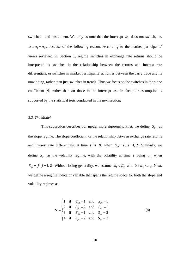
3.2. The Model

This subsection describes our model more rigorously. First, we define tSβ as

the slope regime. The slope coefficient, or the relationship between exchange rate returns

and interest rate differentials, at time t is iβ when tS iβ = , 1, 2i = . Similarly, we

define tSσ as the volatility regime, with the volatility at time t being jσ when

tS jσ = , 1, 2j = . Without losing generality, we assume 1 2β β< and 1 20 σ σ< < . Next,

we define a regime indicator variable that spans the regime space for both the slope and

volatility regimes as

1 if 1 and 12 if 2 and 13 if 1 and 24 if 2 and 2

t t

t tt

t t

t t

S SS S

SS SS S

β σ

β σ

β σ

β σ

= =⎧⎪ = =⎪= ⎨ = =⎪⎪ = =⎩

(8)

11

where tS evolves according to a first-order Markov process with transition probability

matrix P . The ( , )k l element of the transitional matrix klp is the probability of

transition from the regime l to k in a month.

In what follows, we call the regime with 1tSβ = , i.e. a lower slope coefficient

1β , the “Negative” regime, while we call the regime with 2tSβ = the “Positive” regime.

These terms are motivated by the empirical results shown later: the estimates of 1β and

2β are negative and positive, respectively, for all currencies and maturities. Similarly,

the regimes with low and high volatilities, or 1tSσ = and 2tSσ = , are called the “Low”

and “High” regimes, respectively. Accordingly, for instance, the regime with 1tS = , or

1tSβ = and 1tSσ = , is called the “Negative/Low” regime.

In sum, our model can be described as follows:

*, ,( ) 12 / ( )t n t t t n t n t t ny y n r rα β σ η+ +− ⋅ = + − + , (9)

1 1 3 2 2 4( ) ( )t t t t tS S S Sβ β β= + + + , (10)

1 1 2 2 3 4( ) ( )t t t t tS S S Sσ σ σ= + + + , (11)

1ktS = if tS k= , and 0ktS = otherwise; 1, 2, 3, 4k = , (12)

1Pr[ | ]t t klS k S l p+ = = = ; , 1, 2, 3, 4k l = , (13)

4

11kl

kp

=

=∑ , (14)

1 2β β< , (15)

1 20 σ σ< < . (16)

12

Here, t nη + follows (0,1)N , and is independent from 1, ,t tη η − K The model has 21

parameters including α , 1β , 2β , 1σ , 2σ , and a 4 4× transition matrix P . We

should estimate these parameters and the unobservable state variable tS , 1, 2,t = K . We

discuss the estimation strategy in the next subsection.

3.3. Estimation Strategy

To estimate the above model, we employ a Bayesian Gibbs sampling approach,

which is used by, among others, Albert and Chib (1993), Kim, Nelson and Startz (1998),

and Kim and Nelson (1999). Starting from arbitrary initial values of the parameters, the

Gibbs sampling proceeds by taking the following steps:

Step 1: A drawing from the conditional distribution of the state tS ,

1, 2, 3,t = K , given α , 1β , 2β , 1σ , 2σ , the monthly transition matrix P , and the

monthly data ty , ,t nr , and *,t nr , 1, 2, 3,t = K

Step 2: A drawing from the conditional distribution of P , given α , 1β , 2β ,

1σ , 2σ , and the monthly state and data tS , ty , ,t nr , and *,t nr , 1, 2, 3,t = K

Step 3: A drawing from the conditional distribution of 1σ , given α , 1β , 2β ,

2σ , the n -month transaction matrix nP , and the every n -month state and data tS , ty ,

,t nr , and *,t nr , 1, 1 ,1 2 ,t n n= + + K

Step 4: A drawing from the conditional distribution of 2σ , given α , 1β , 2β ,

13

1σ , nP , and the every n -month state and data.

Step 5: A drawing from the conditional distribution of α , given 1β , 2β , 1σ ,

2σ , nP , and the every n -month state and data.

Step 6: A drawing from the conditional distribution of 1β , given α , 2β , 1σ ,

2σ , nP , and the every n -month state and data.

Step 7: A drawing from the conditional distribution of 2β , given α , 1β , 1σ ,

2σ , nP , and the every n -month state and data.

By iterating these steps successively, we simulate a drawing from the joint

distribution of the state variable and parameters of the model, given the data. It is then

straightforward to summarize the marginal distributions of any of these, given the data.

Although this Gibbs sampling is just a simple extension of the methods

employed in the literature, there is an important new aspect. In steps 1 and 2, we generate

the state variable and transaction matrix from their conditional distributions, given the

monthly data and/or state. Nevertheless, in steps 3 through 7, we generate α , 1β , 2β ,

1σ , and 2σ , given the every- n -month, i.e. quarterly or semiannual data and state. In the

later steps, we use the lower-frequency state and data to avoid possible estimation biases

arising from using overlapping data. On the other hand, since we use the monthly states

and data in steps 1 and 2, we can examine the properties of higher-frequency state

transitions.

We employ diffuse or non-informative priors for all the parameters of the model

as ~ (0,10)Nα , 1 ~ ( 1,10)Nβ − , 2 ~ (1,10)Nβ , 21 ~ (4,300)IGσ , 2 2

2 1/ ~ (4,8)IGσ σ ,

14

and 1 4 0, 1 0, 4( , ) ~ ( , )k k k kp p Dirichlet p pK K where 0, 4kkp = and 0, 1klp = if k l≠ .

Data that we use in estimating the regime-switching model are monthly and exactly the

same as those obtained for the OLS analysis in Section 2.

4. Results

This section discusses the estimation results of our regime-switching model.

First, subsection 4.1 statistically confirms that our model is appropriate in comparison

with alternative models to explain the relationship between exchange rates and interest

rate differentials. We then discuss the parameter estimates in subsection 4.2. Finally,

subsection 4.3 investigates the regime probabilities and transition matrices to understand

how the slope and volatility regimes are related to each other.

4.1. Model Comparison

This subsection statistically confirms that our model is appropriate in

comparison with three alternatives. The first alternative model is called the “unrestricted

2 2× regime model,” which is less restricted than our model in the sense that the

intercept parameter α is allowed to switch simultaneously with the slope coefficient

β . The second alternative is called the “independent 2 2× regime model,” in which the

slope and volatility regimes are restricted to be perfectly independent similar to the

models employed by Bollen, Gray and Whaley (2000) and Dewachter (2004). The last

one is called the “2 regime model,” in which the slope and volatility regimes are

restricted to switch simultaneously similar to the model employed by Engel and

15

Hamilton (1990) and Engel (1994). Note that the last two alternative models are less

restricted than the models in the literature, in the sense that the slope coefficients are not

assumed to be zero.

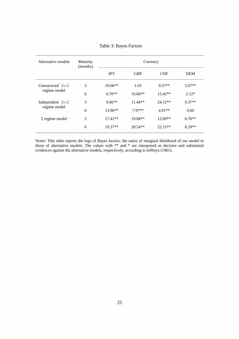
For the comparison between our model and these alternatives, we use a Bayes

factor, the ratio of the marginal likelihood of our model to the marginal likelihood of

each alternative. With this definition, if the logs of Bayes factors are positive, we can

interpret our model as being supported. To calculate the Bayes factors, we employ Chib’s

(1995) method, and the logs of them are reported in Table 3. This table shows that they

are positive in all 24 cases, i.e. for all alternative models, currencies, and maturities, and

that our model dominates the alternatives. Moreover, in 22 out of 24 cases, they are

larger than 4.61, which is interpreted as decisive evidence against the alternative models,

according to Jeffreys (1961). The evidence against the unrestricted 2 2× regime model

implies that allowing the intercept parameter to switch does not improve the model’s

ability to explain exchange rate returns. This implies that regime switches in exchange

rate returns should be interpreted as switches in the relationship between the returns and

interest rate differentials as viewed by market participants. The evidence against the other

two alternative models implies that the slope and volatility regimes are not perfectly

independent nor dependent.

4.2. Parameter Estimates

The preceding subsection confirmed that our model performs better than the

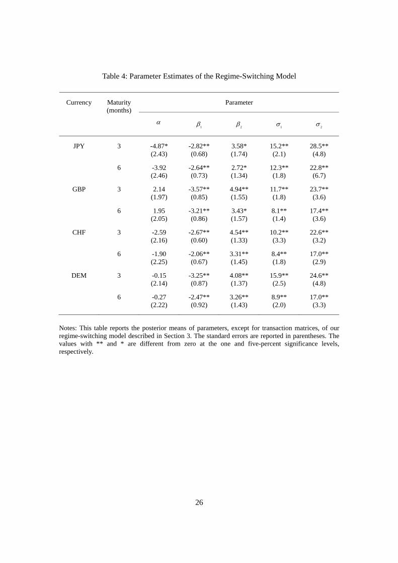
alternatives. Here we discuss the estimation results of this model. Table 4 reports the

posterior means of parameters except for transition matrices, and shows that the slope

16

coefficients 1β and 2β are negative and positive, respectively, in all cases. According

to the posterior distributions, all of the slope coefficients are different from zero at the

five-percent significance level. In addition, the point estimates of 2β are larger than

those of 1β in absolute values in all eight cases. This implies that the appreciation of

low-interest-rate currencies is faster than the depreciation. On the other hand, according

to Table 5, which reports the unconditional probabilities of the Negative and Low

regimes calculated with eigenvectors of transition matrices, the probabilities of the

Negative regime are higher than 50 percent in all eight cases, and reach to 66 percent on

average.

All these results imply that low-interest-rate currencies appreciate less

frequently, but once it occurs, its movement is faster than when they depreciate. This

implication, in fact, is less evident for longer maturities, for which the absolute values of

β ’s and the unconditional probabilities of the Negative regime are smaller for all four

currencies.

These results may be interpreted as the exchange rates being influenced by the

carry trade and its unwinding. That is, the depreciation of lower-interest-rate currencies,

or UIP failure, is influenced by the carry trade, while the fast appreciation is influenced

by its rapid unwinding. This is consistent with currency traders’ views described as

“going up by the stairs and coming down in the elevator” (see Breedon (2001) and

Plantin and Shin (2006)).

Table 4 also shows that the higher volatility 2σ is around twice the lower

volatility 1σ . In fact, they are different at the five-percent significance level in all cases.

This table also shows that the volatilities are lower for longer maturities, and this may

17

reflect a mean-reverting nature in exchange rates.

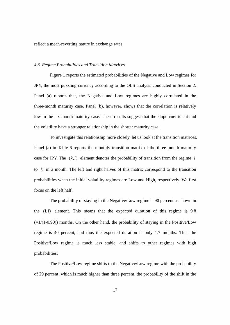
4.3. Regime Probabilities and Transition Matrices

Figure 1 reports the estimated probabilities of the Negative and Low regimes for

JPY, the most puzzling currency according to the OLS analysis conducted in Section 2.

Panel (a) reports that, the Negative and Low regimes are highly correlated in the

three-month maturity case. Panel (b), however, shows that the correlation is relatively

low in the six-month maturity case. These results suggest that the slope coefficient and

the volatility have a stronger relationship in the shorter maturity case.

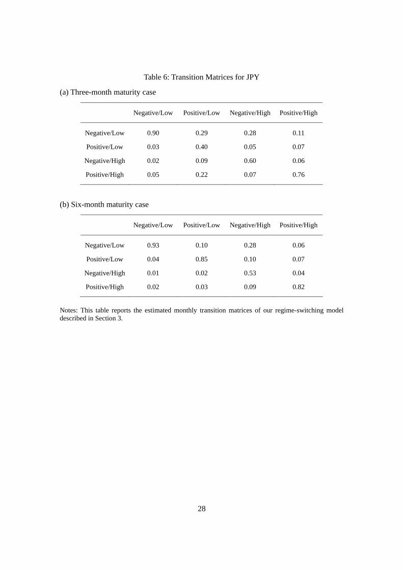
To investigate this relationship more closely, let us look at the transition matrices.

Panel (a) in Table 6 reports the monthly transition matrix of the three-month maturity

case for JPY. The ( , )k l element denotes the probability of transition from the regime l

to k in a month. The left and right halves of this matrix correspond to the transition

probabilities when the initial volatility regimes are Low and High, respectively. We first

focus on the left half.

The probability of staying in the Negative/Low regime is 90 percent as shown in

the (1,1) element. This means that the expected duration of this regime is 9.8

(=1/(1-0.90)) months. On the other hand, the probability of staying in the Positive/Low

regime is 40 percent, and thus the expected duration is only 1.7 months. Thus the

Positive/Low regime is much less stable, and shifts to other regimes with high

probabilities.

The Positive/Low regime shifts to the Negative/Low regime with the probability

of 29 percent, which is much higher than three percent, the probability of the shift in the

18

reverse direction. That is, the slope regime tends to converge into the Negative regime as

long as the volatility is low. This implies that the Negative regime tends to occur in a

low-volatility environment, not only because the probability of staying in the

Negative/Low regime is high but also because the Positive regime shifts to the Negative

regime with a high probability.

The other reason why the probability of staying in the Positive/Low regime is

lower than in the Negative/Low regime is that the volatility increases more easily under

this regime. The probability of shift from the Positive/Low regime to the Positive/High or

Negative/High regime, which is calculated as the sum of (3,2) and (4,2) elements, is 31

percent, and is much higher than seven percent, the probability of shift from the

Negative/Low regime to the Positive/High or Negative/High regime. This result implies

that lower volatility is easier to be maintained under the Negative regime rather than

under the Positive regime.

All the results in this subsection suggest that UIP failure and a low-volatility

environment are mutually dependent. This sharp contrast in stability between the

Negative and Positive regimes, however, is not seen clearly in the right half of Panel (a)

and the whole Panel (b), i.e. when the volatility is higher or maturities are longer.

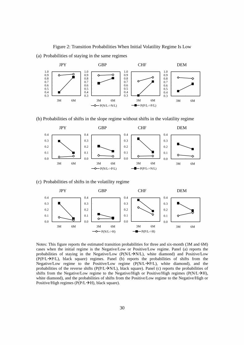
Figures 2 and 3 confirm that these implications of Table 6 hold for all currencies.

Figure 2 depicts the estimated transition probabilities when the initial volatility regime is

Low. Panel (a) shows that the probabilities of staying in the Positive/Low regime in the

next month are lower than the probabilities of staying in the Negative/Low regime for all

four currencies and maturities. This difference in probabilities is much larger for the

three-month cases. Panels (b) and (c) show that the probabilities of shift from the

19

Positive/Low regime to the other regimes are high, especially for the shorter maturities.

In contrast, Figures 3 shows that these properties are not observed when the initial

volatility regime is High.

5. Conclusion

Lower-interest-rate currencies tend to depreciate against higher-interest-rate

currencies. This observation is in opposition to what is predicted by UIP, and, according

to many market participants’ views, this may be caused by the carry-trade activities in a

low-volatility environment. We use OLS regressions and a regime-switching model to

examine how exchange rate volatilities and UIP failure are related to each other. The

regime-switching model allows the slope regime, which governs the relationship between

exchange rate returns and interest rate differentials, and the volatility regime to be not

perfectly independent nor dependent. This property of the model enables us to investigate

the relationship among exchange rate returns, volatilities, and interest rate differentials.

We estimate this model using a Bayesian Gibbs sampling approach, in which the

states and transition matrices are generated conditional on the monthly data and/or state,

while the parameters of intercept, slope coefficient, and volatility are generated

conditional on the quarterly or semiannual data and state. With this method, we can

examine the state transitions in a high frequency, while avoiding possible estimation

biases arising from overlapping data.

The main findings are as follows. First, statistical tests using Bayes factors

support our model in comparison with the alternatives. The evidence suggests that regime

20

switches in exchange rate returns should be interpreted as switches in the relationship

between the returns and interest rate differentials without switches in trends of exchange

rate. The evidence also implies that the slope and volatility regimes are partially

dependent; we should not assume that the regimes are perfectly independent or

dependent.

Second, low-interest-rate currencies appreciate less frequently, but once it

occurs, its movement is faster than when they depreciate. This may be because the

appreciation is influenced by a rapid unwinding of the carry trade.

Third, a low volatility tends to cause UIP failure, and this may be because a

higher Sharpe ratio attracts investors to the carry trade. In fact, the reverse is also true.

That is, UIP failure tends to cause a lower-volatility environment, which may imply that

a high volatility does not tend to occur until an unwinding of the carry trade. These

results imply that the low-volatility environment and UIP failure are mutually dependent,

and the stability would be lost once the slope or volatility regime shifts.

Finally, the second and third findings are more evident for shorter maturities,

and this may imply that UIP failure is influenced by short-term carry trade activities.

21

References

Albert, J.H., Chib, S., 1993. Bayes inference via Gibbs sampling of autoregressive time series subject to Markov mean and variance shifts. Journal of Business and Economic Statistics 11 (1), 1-15.

Alexius, A., 2001. Uncovered interest rate parity revisited. Review of International Economics 9, 505-517.

Alvarez, F., Atkeson, A., Kehoe, P.J., 2005. Time-varying risk, interest rates, and exchange rates in general equilibrium. Federal Reserve Bank of Minneapolis Working Paper 627.

Bekaert, G., Hodrick, B., 1993. On biases in the measurement of foreign exchange risk premiums. Journal of International Money and Finance 12, 115-138.

Bollen, N.P.B., Gray, S.F., Whaley, R.E., 2000. Regime switching in foreign exchange rates: Evidence from currency option prices. Journal of Econometrics 94, 29-276.

Breedon, F., 2001. Market liquidity under stress: observations in the FX market. Lehman Brothers working paper, presented at the BIS workshop on market liquidity http://www.bis.org/publ/bispap02g.pdf.

Burnside, C., Eichenbaum, M., Kleshchelski, I., Rebelo, S., 2006. The returns of currency speculation. NBER working paper 12489.

Chib, S., 1995. Marginal likelihood from the Gibbs output. Journal of the American Statistical Association 90, 1313-1321.

Chinn M.D., G. Meredith, 2004. Monetary policy and long-horizon uncovered interest rate parity. IMF Staff Papers 51, 409-430.

Dewachter H., 2001. Can Markov switching models replicate chartist profits in the foreign exchange market? Journal of International Money and Finance 20, 25-41.

Engel, C., Hamilton, J.D. 1990. Long swings in the dollar: Are they in the data and do markets know it? American Economic Review 80, 689-713.

Engel, C., 1994. Can the Markov switching model forecast rates? Journal of International Economics 36, 151-165.

Fama, E.F., 1984. Forward and spot exchange rates. Journal of Monetary Economics 14,

22

319-338.

Hamilton, J.D., 1989. A new approach to the economic analysis of nonstationary time series and the business cycle. Econometrica 57, 357-384.

Jeffreys, H., 1961. Theory of Probability, 3rd edition, Oxford University Press, New York.

Kim, C., Nelson, C., Startz, R., 1998. Testing for mean reversion in Heteroskedastic data based on Gibbs-sampling-augmented randomization. Journal of Empirical Finance 5, 131-154.

Kim, C., Nelson, C., 1999. Has the U.S. economy become more stable? A Bayesian approach based on a Markov-switching model of the business cycle. Review of Economics and Statistics 81 (4), 608-616.

Lusting, H., Verdelhan, A., 2007. The cross-section of foreign currency risk premia and consumption growth risk. American Economic Review, forthcoming.

Plantin, G., Shin, H.S., 2006. Carry trades and speculative dynamics. Working paper.

de Rato, R., 2007. Speech by Rodrigo de Rato, Managing Director of the IMF, the Harvard business school alumni dinner. Downloaded from IMF web site, http://www.imf.org/external/speeches/2007/022607.html.

23

Table 1: Results of UIP Test Regressions

Currency Maturity (months)

JPY GBP CHF DEM

3 -2.82** -1.94* -1.32 -0.60 (0.87) (0.87) (0.69) (0.80)

6 -2.36** -1.61 -0.97 -0.61 (0.91) (0.92) (0.74) (0.88)

Notes: This table reports the regression estimates of the slope coefficient in equation (2). The standard errors are reported in parentheses. The values with ** and * are different from zero at the one and five-percent significance levels, respectively. The sample is January 1980 to April 2000 for DEM, and to May 2007 for the others.

24

Table 2: UIP Failure and Exchange Rate Volatility

Currency Maturity (months)

JPY GBP CHF DEM

3 0.53** 0.34* 0.43** 0.22 (0.13) (0.16) (0.14) (0.21)

6 0.52** 0.53** 0.24 -0.04 (0.18) (0.17) (0.18) (0.28)

Notes: This table reports the regression estimates of vβ in equation (3). The standard errors are reported in parentheses. The values with ** and * are different from zero at the one and five-percent significance levels, respectively. The sample is January 1980 to April 2000 for DEM, and to May 2007 for the others.

25

Table 3: Bayes Factors

Currency Alternative models Maturity (months)

JPY GBP CHF DEM

3 19.06** 1.03 9.57** 5.97** Unrestricted 2 2× regime model

6 6.70** 16.66** 15.42** 2.12*

3 9.66** 11.44** 24.12** 9.37** Independent 2 2× regime model

6 13.96** 7.97** 4.91** 0.60

3 17.41** 19.84** 12.69** 6.76** 2 regime model

6 19.37** 28.54** 22.15** 8.29**

Notes: This table reports the logs of Bayes factors, the ratios of marginal likelihood of our model to those of alternative models. The values with ** and * are interpreted as decisive and substantial evidences against the alternative models, respectively, according to Jeffreys (1961).

26

Table 4: Parameter Estimates of the Regime-Switching Model

Currency Parameter

Maturity (months)

α 1β 2β 1σ 2σ

JPY 3 -4.87* -2.82** 3.58* 15.2** 28.5** (2.43) (0.68) (1.74) (2.1) (4.8)

6 -3.92 -2.64** 2.72* 12.3** 22.8** (2.46) (0.73) (1.34) (1.8) (6.7)

GBP 3 2.14 -3.57** 4.94** 11.7** 23.7** (1.97) (0.85) (1.55) (1.8) (3.6)

6 1.95 -3.21** 3.43* 8.1** 17.4** (2.05) (0.86) (1.57) (1.4) (3.6)

CHF 3 -2.59 -2.67** 4.54** 10.2** 22.6** (2.16) (0.60) (1.33) (3.3) (3.2)

6 -1.90 -2.06** 3.31** 8.4** 17.0** (2.25) (0.67) (1.45) (1.8) (2.9)

DEM 3 -0.15 -3.25** 4.08** 15.9** 24.6** (2.14) (0.87) (1.37) (2.5) (4.8)

6 -0.27 -2.47** 3.26** 8.9** 17.0** (2.22) (0.92) (1.43) (2.0) (3.3)

Notes: This table reports the posterior means of parameters, except for transaction matrices, of our regime-switching model described in Section 3. The standard errors are reported in parentheses. The values with ** and * are different from zero at the one and five-percent significance levels, respectively.

27

Table 5: Unconditional Probabilities of the Negative and Low Regimes

Currency

Maturity (months)

JPY GBP CHF DEM

Negative 3 0.72 0.79 0.61 0.62

6 0.63 0.75 0.59 0.56

Low 3 0.70 0.58 0.29 0.63

6 0.85 0.64 0.42 0.39

Notes: This table reports the unconditional probabilities of regimes, which are calculated using eigenvectors of estimated transition matrices.

28

Table 6: Transition Matrices for JPY

(a) Three-month maturity case

Negative/Low Positive/Low Negative/High Positive/High

Negative/Low 0.90 0.29 0.28 0.11

Positive/Low 0.03 0.40 0.05 0.07

Negative/High 0.02 0.09 0.60 0.06

Positive/High 0.05 0.22 0.07 0.76

(b) Six-month maturity case

Negative/Low Positive/Low Negative/High Positive/High

Negative/Low 0.93 0.10 0.28 0.06

Positive/Low 0.04 0.85 0.10 0.07

Negative/High 0.01 0.02 0.53 0.04

Positive/High 0.02 0.03 0.09 0.82

Notes: This table reports the estimated monthly transition matrices of our regime-switching model described in Section 3.

29

Figure 1: Regime Probabilities for JPY

(a) Three-month maturity case

00.10.20.30.40.50.60.70.80.9

1

80 82 84 86 88 90 92 94 96 98 00 02 04 06

Low Negative

(b) Six-month maturity case

00.10.20.30.40.50.60.70.80.9

1

80 82 84 86 88 90 92 94 96 98 00 02 04 06

Low Negative

Notes: This figure shows the estimated probabilities of the Negative (thick line) and Low (shadow) regimes for the Japanese yen. The sample is from January 1980 to May 2007.

30

Figure 2: Transition Probabilities When Initial Volatility Regime Is Low

(a) Probabilities of staying in the same regimes

JPY GBP CHF DEM

0.30.40.50.60.70.80.91.0

3M 6MP(N/L->N/L)

0.30.40.50.60.70.80.91.0

3M 6MP(P/L->P/L)

0.30.40.50.60.70.80.91.0

3M 6M0.30.40.50.60.70.80.91.0

3M 6M

(b) Probabilities of shifts in the slope regime without shifts in the volatility regime

JPY GBP CHF DEM

0.0

0.1

0.2

0.3

0.4

3M 6MP(N/L->P/L)

0.0

0.1

0.2

0.3

0.4

3M 6MP(P/L->N/L)

0.0

0.1

0.2

0.3

0.4

3M 6M0.0

0.1

0.2

0.3

0.4

3M 6M

(c) Probabilities of shifts in the volatility regime

JPY GBP CHF DEM

0.0

0.1

0.2

0.3

0.4

3M 6MP(N/L->H)

0.0

0.1

0.2

0.3

0.4

3M 6MP(P/L->H)

0.0

0.1

0.2

0.3

0.4

3M 6M0.0

0.1

0.2

0.3

0.4

3M 6M

Notes: This figure reports the estimated transition probabilities for three and six-month (3M and 6M) cases when the initial regime is the Negative/Low or Positive/Low regime. Panel (a) reports the probabilities of staying in the Negative/Low (P(N/L N/L), white diamond) and Positive/Low (P(P/L P/L), black square) regimes. Panel (b) reports the probabilities of shifts from the Negative/Low regime to the Positive/Low regime (P(N/L P/L), white diamond), and the probabilities of the reverse shifts (P(P/L N/L), black square). Panel (c) reports the probabilities of shifts from the Negative/Low regime to the Negative/High or Positive/High regimes (P(N/L H), white diamond), and the probabilities of shifts from the Positive/Low regime to the Negative/High or Positive/High regimes (P(P/L H), black square).

31

Figure 3: Transition Probabilities When Initial Volatility Regime Is High

(a) Probabilities of staying in the same regimes

JPY GBP CHF DEM

0.30.40.50.60.70.80.91.0

3M 6MP(N/H->N/H)

0.30.40.50.60.70.80.91.0

3M 6MP(P/H->P/H)

0.30.40.50.60.70.80.91.0

3M 6M0.30.40.50.60.70.80.91.0

3M 6M

(b) Probabilities of shifts in the slope regime without shifts in the volatility regime

JPY GBP CHF DEM

0.0

0.1

0.2

0.3

0.4

3M 6MP(N/H->P/H)

0.0

0.1

0.2

0.3

0.4

3M 6MP(P/H->N/H)

0.0

0.1

0.2

0.3

0.4

3M 6M0.0

0.1

0.2

0.3

0.4

3M 6M

(c) Probabilities of shifts in the volatility regime

JPY GBP CHF DEM

0.0

0.1

0.2

0.3

0.4

3M 6MP(N/H->L)

0.0

0.1

0.2

0.3

0.4

3M 6MP(P/H->L)

0.0

0.1

0.2

0.3

0.4

3M 6M0.0

0.1

0.2

0.3

0.4

3M 6M

Notes: This figure reports the estimated transition probabilities for three and six-month (3M and 6M) cases when the initial regime is the Negative/High or Positive/High regime. Panel (a) reports the probabilities of staying in the Negative/High (P(N/H N/H), white diamond) and Positive/High (P(P/H P/H), black square) regimes. Panel (b) reports the probabilities of shifts from the Negative/High regime to the Positive/High regime (P(N/H P/H), white diamond), and the probabilities of the reverse shifts (P(P/H N/H), black square). Panel (c) reports the probabilities of shifts from the Negative/High regime to the Negative/Low or Positive/Low regimes (P(N/H L), white diamond), and the probabilities of shifts from the Positive/High regime to the Negative/Low or Positive/Low regimes (P(P/H L), black square).