Long Horizon Uncovered Interest Parity Re Assessed · Long Horizon Uncovered Interest Parity Re ......

0

Long Horizon Uncovered Interest Parity Re‐Assessed

By

Menzie D. Chinn

and

Saad Quayyum

October 4, 2013

Abstract

We review the evidence for both short and long horizon uncovered interest parity (UIP) and rational

expectations over the period up to 2011, extending the sample examined in Chinn and Meredith (2004)

by nearly a decade. We find that the joint hypothesis of UIP and rational expectations (known as the

unbiasedness hypothesis) holds better at long horizons than at short, although the effect is somewhat

weaker than documented in Chinn and Meredith (2004). Using the formula for the slope coefficient, we

identify potential sources for the difference in slope coefficients at different horizons. We attribute our

weaker findings for long horizon unbiasedness for certain currencies partly to the advent of

extraordinarily low interest rates associated with the zero interest bound in Japan and Switzerland.

JEL classification: F31, F41

Keywords: uncovered interest parity, unbiasedness hypothesis, rational expectations, exchange rates, financial

market integration, emerging markets

Acknowledgments: We thank Charles Engel, Joe Gagnon and Ken West for helpful comments. The

financial support of University of Wisconsin graduate research funds is gratefully acknowledged by

Chinn.

* Robert M. La Follette School of Public Affairs; and Department of Economics, University of Wisconsin,

1180 Observatory Drive, Madison, WI 53706‐1393. Email: mchinn [at] lafollette.wisc.edu

** IMF, Washington, D.C. 20431. Email: squayyum [at] imf.org

1

1. Introduction

The failure of the joint hypothesis of uncovered interest rate parity (UIP) and rational

expectations is one of the most robust empirical regularities – and puzzles – in international finance.

According to the unbiasedness hypothesis, the interest rate differential between two countries should

be an unbiased predictor of the change in the exchange rate between them. As Chinn and Meredith

(2004) document, in a sample extending up to 2000, this hypothesis holds at longer horizons of five and

ten years, while failing to hold at shorter horizons extending up to a year.

This paper revisits the question of whether unbiasedness holds at long horizons, extending the

Chinn and Meredith (2004) dataset to 2011. Prior to Chinn and Meredith (2004), most papers focused

on the UIP hypothesis over short horizons of less than one year. This reflected the difficulty in obtaining

constant maturity longer term yields and the relatively short sample (relative to bond maturities)

available during the floating rate period.1 We now have a longer sample with which to conduct our

analyses, and therein lies the hope of estimating the relevant parameters more precisely.

However, data issues are not the only, or even primary reasons for this revisit. We believe a re‐

examination is important for at least four additional reasons. First, the last decade includes a period in

which short rates have effectively hit the zero interest rate bound. While long term rates remain above

zero, they remain quite low by historical standards, particularly for Japan and Switzerland. Second, the

2000’s were an era marked by unprecedented purchases of government bonds by the official sector

(specifically, East Asian and oil‐exporter central banks). It is unclear to us that UIP should hold under

such circumstances. Third, there is evidence that some factors that have typically been ignored, such as

1 Fixed or constant maturity yields for specified horizon are synthetic yields derived from yields of bonds with maturity shorter and longer than the specified horizon. Say we are interested in getting yield of a bond than expires in exactly ten years from today. It is unlikely that there is a government bond out there in the market which expires exactly 10 years from today. However there are bonds in the marker that expire in more than 10 years and less than ten years. The constant maturity 10 year yield data is calculated from the yields of these bonds.

2

default risk, have become increasingly important since the financial crisis of 2008; since covered interest

parity is a prerequisite for uncovered interest parity to hold, there is reason to believe that the behavior

of deviations from parity has changed. Finally, it is of interest to see if our previous conclusions

regarding this hypothesis have been colored by the behavior of Deutschemark. To the extent that the

DM and other legacy currencies no longer exist, the characterization of currency behavior should be

adapted to reflect these new realities.

To anticipate our results, we obtain the following findings. First, we find that UIP still holds

better at long horizons than at short, although the effect is somewhat weaker than documented in

Chinn and Meredith (2004). Second, the results are sensitive to the bond yields used. Third, the failure

of the unbiasedness hypothesis is more pronounced at long horizons when using the pound, instead of

the dollar, as the base currency. Finally, for the currencies characterized by particularly low bond yields

– the Japanese yen and the Swiss franc, interest rates in the mid‐1990’s onward do not point in the right

direction for subsequent exchange rate changes. In other words, the advent of extraordinarily low

interest rates associated with the advent of the zero interest bound in Japan and Switzerland seems to

have attenuated the long horizon unbiasedness effect.

In the next section we briefly explore the literature. In Section 3 we review the unbiasedness

hypothesis and the underlying assumptions behind it. In Section 4, we look at the empirical evidence at

short and long horizons respectively. In Section 5 we explore theoretical reasons behind our main

empirical finding. Section 6 includes some robustness tests. In Section 7 we conclude.

2. Theory and Literature

UIP is a parity relationship built up on a number of assumptions. It is convenient to start with the

covered interest parity (CIP) relationship. CIP states that with efficient financial market with no default

risk and no barriers to capital flows, the no arbitrage condition is that the k period ahead forward

3

exchange rate at time t, , ) can be expressed as a function of nominal rate of returns on risk free

bonds that matures in period k and the spot exchange rate as follows:

, ,

,∗ (1)

where is the spot exchange rate at time t expressed as home currency units per unit of foreign

currency. , is the gross return (one plus the yield) on a default risk free bond denominated in the

home currency that matures in period k, and ,∗ is the corresponding gross return denominated in

foreign currency. The above relationship has been found to generally hold empirically.2 Taking logs, the

above expression can be approximated as:

, , ,∗ (2)

where the lower scripts signifies logs of the variables described above.

The forward exchange rate is merely the price of foreign exchange set for a trade k periods ahead,

determined in the market at time t, that makes the returns equal when expressed in a common

currency.

How market participants determine the forward rate is not explained in this parity condition.

Under certain conditions, most importantly risk neutrality, the forward rate can be interpreted as the

expected future spot exchange rate.3 If investors are risk averse, the forward rate will differ from the

expected future spot exchange rate by amount of the risk premium, which we can define as follows:

, , (3)

2 See Dooley and Isard (1980) for discussion, and Popper (1993) for a review of the literature, and long horizon findings. 3 See Engel (1996) for a discussion of how the forward rate and the expected spot rate might deviate even under rational expectations and risk neutrality.

4

Where , is the exchange risk premium, and is the subjective expectation of the future spot

rate based on time t information. Substituting equations (3) into equation (2), one obtains the following

expression:

, ,∗ , (4)

Equation (4) relates ex ante depreciation to the interest differential (the term in the parentheses) and

the exchange risk premium.

The UIP hypothesis states, if investors are risk neutral, the return from investing a unit amount

in a risk free bond in the home currency for period k, , , should equal the expected return from

converting the unit amount into foreign currency and investing in risk free bond in foreign currency for

period k, and converting the foreign currency return back into home currency after period k. In equation

(5) this implies that the , term is zero.

Of course this hypothesis is difficult to test since one doesn’t directly observe the market’s

subjective expectations. Hence, researchers typically adopt the rational expectations hypothesis, so that

the subjective market expectation equals the mathematical (conditional) expectation. Under the

rational expectations hypothesis, the actual value of the future spot rate equals the expected value of

future spot rate plus an error term,

, (5)

where is an expectation error which is orthogonal to everything that is known at time t. This yields:

, ,∗ , (6)

The resulting unbiasedness hypothesis is usually tested using the following specification, often referred

to as the “Fama regression” (Fama, 1984):

5

, ,∗ (7)

where the expected value of according to the hypothesis is 1. The maintained hypothesis is the null

hypothesis, and under the unbiasedness null, the error is merely the expectations error, and is

orthogonal to the interest rate differential, , ,∗ . (Under the alternative, could be an error

term that does not fulfill the rational expectations criteria, and/or a time varying risk premium, possibly

correlated with the interest differential.) Note in the regressions reported in this paper, the exact

formulas are used instead of the log approximations.

Note that the intercept may be non zero while testing for UIP using equation (7). A non zero

alpha may reflect a constant risk premium (hence, we are really testing for a time‐varying risk premium,

rather than risk neutrality per se) and/or approximation errors stemming from Jensen’s Inequality from

the fact that expectation of a ratio (the exchange rate) is not equal to the ratio of the expectation.

The literature testing variants of the uncovered interest rate parity hypothesis at short horizons

is enormous. Most of the studies fall into the category employing the rational expectations hypothesis;

in our lexicon, that means they are tests of the unbiasedness hypothesis. Estimates of equation (6) using

values for k that range up to one year typically reject the unbiasedness restriction on the slope

parameter. For instance, the survey by Froot and Thaler (1990), for instance, finds an average estimate

for β of ‐0.88.4 Bansal and Dahlquist (2000) provide more mixed results, when examining a broader set

of advanced and emerging market currencies. They also note that the failure of unbiasedness appears to

depend upon whether the US interest rate is above or below the foreign.5 Frankel and Poonawala (2010)

4 Similar results are cited in surveys by MacDonald and Taylor (1992) and Isard (1995). Meese and Rogoff (1983) show that the forward rate is outpredicted by a random walk, which is consistent with the failure of the unbiasedness hypothesis. 5 Flood and Rose (1996, 2002) note that including currency crises and devaluations, one finds more evidence for the unbiasedness hypothesis.

6

show that for emerging markets more generally, the unbiasedness hypothesis coefficient is typically

more positive.6

The earliest studies that explored the UIP hypothesis over long horizons include Flood and

Taylor (1997) and Alexius (2001). Flood and Taylor (1997) explores the UIP relationship at three year

horizon pooling 21 currencies of mostly developed countries, with the U.S. Dollar as the base currency.

They estimate to be 0.596 with a standard error of 0.195. However, the bond yields used are

heterogeneous, with varying maturities, so are difficult to interpret. Alexius (2001) finds evidence of UIP

holding at long horizon using 14 long term bonds of varying maturities, using a sample from 1957‐97. As

the sample encompasses the Bretton Woods era and the associated capital control regime, those

findings are perhaps not applicable in current times.

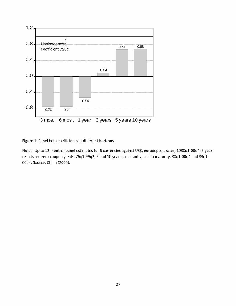
Chinn and Meredith (2004) tested the UIP hypothesis at five year and ten year horizons for the

Group of Seven (G7) countries, and found greater support for the UIP hypothesis holding at these long

horizons than in shorter horizons of three to twelve months. The estimated coefficient on the interest

rate differentials were positive and were closer to the value of unity than to zero in general. The sample

used in that paper extended up to 2000. The panel findings are summarized in Figure 1.

Madarassy and Chinn (2002) document additional positive evidence of long horizon

unbiasedness for some non‐G7 currencies. In contrast, Bekaert, Wing and Xie (2007) fails to find

evidence that unbiasedness holds better at long horizons.

6 There is an alternative approach that involves using survey‐based data to measure exchange rate expectations. Chinn and Frankel (1994) document that it is difficult to reject UIP for a broad set of currencies when using survey based forecasts. Similar results are obtained by Chinn (2012), when extending the data up to 2009. These results echo early findings by Froot and Frankel (1989). While we do not pursue this avenue in this paper (long horizon expectations being difficult to obtain), it is useful to recall these findings when interpreting rejections of the joint hypothesis of UIP and rational expectations.

7

3. Unbiasedness Estimated at Short and Long Horizons

In this paper we extend the sample up to 2011 and re‐test the unbiasedness hypothesis using equation 7

both at the short and long horizons.7 Among the G7 countries, Italy, France and Germany adopted the

Euro, so the UIP regression on the Italian Lira, French Franc and German Mark could not be extended.

The Euro has too short a history to be tested at long horizon. Thus we were left with the U.S. Dollar,

Japanese Yen, Canadian Dollar and British Pound for our analysis. We include results for the euro at the

short horizon. And to this group of currencies we added the Swiss Franc for which we were able to find

constant maturity yields at long horizons.

3.1 The Short Horizon

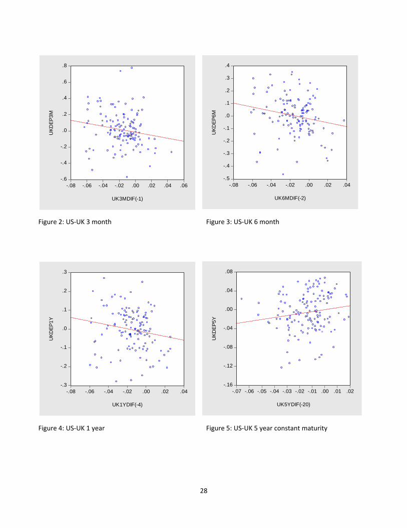
The stylized facts regarding exchange rate changes and interest differentials are well known. Ex post

exchange rate changes are highly variable, while interest differentials are not, and visually exhibit almost

no relationship with subsequent changes. For illustrative purposes, we display in Figures 2‐4 the interest

rates and exchange rate changes (timed appropriately) for the US dollar‐British pound pair at the three,

six and twelve month horizons, starting from 1979:Q1, and running through 2011:Q4. The , and ,∗

are returns from deposits in the Eurocurrency markets for maturities of three, six and twelve months

taken from Bloomberg. The data are sampled at quarterly frequencies with exchange rate and yield

observations recorded at the end of the quarter. A simple OLS regression line is included. Note that, in

line with the findings in the literature, the best‐fit line is downward sloping. This characterization is true

for the other currency pairs.8

In Table 1, we quantify the extent of the downward slope, and present the OLS estimates of

obtained from estimating equation 7 for horizons of three, six months and twelve months. The standard

7 Note in the regressions reported in this paper, the exact formulas are used instead of the log approximations. 8 Note that in Chinn and Meredith (2004), the same cannot be said for the US dollar‐French franc and US dollar‐Italian lire pairs.

8

errors presented are Newey‐West standard errors, correcting for moving average serial correlation in

the error term up to 2×(k‐1) lags, following Cochrane’s (1991). This means we have used the most

conservative assumptions in terms of the degree of serial correlation.

The interest rate data start from the first quarter of 1979 for the U.S. Dollar, the Canadian

Dollar, the British Pound and the Japanese Yen. For the Swiss Franc the 3‐month data begins from

1991:Q2, the 6‐month data begins from 1996:Q4 and the 12‐month data begins from 1997:Q1. The euro

data begins in 1999Q1.

The two panels contain the regression results with different base (home) currencies. In Panel A

the base currency is the U.S. Dollar. In Panel B the base currency is the British Pound. Note that when

testing the unbiasedness hypothesis for the two currencies in a regression setting, the choice of the

base currency can affect the estimate of .9 However, these differences are not substantial; that is why

we report the regression results for the exchange rate expressed as USD/GBP, but do not report the

corresponding results for GBP/USD.

First note that all the point estimates of are negative. In most of the case the estimates of

are significantly different from one. The exceptions are the USD/CAD in Panel A, and the euro in both

panels. In the latter case, the relatively small sample explains the failure to reject the unbiasedness null;

the standard errors are relatively large.

In the last two row of each panel, we present estimates from constrained panel regression,

where the data for different currencies (with the exception of the Swiss Franc and the euro) are pooled

together and the estimates of for all currencies are constrained to be equal to each other. The

regression controls for country fixed effects, thus allowing a different intercept (or for each country.

Pooling increases the number of observations and allows for more precise estimates of coefficients and

9 When using the exact formula, instead of the log approximations.

9

standard errors. The estimates of in the pooled regression are negative and different from one at the

one percent significance level for all base currency and horizons.

These estimates of are consistent to what has been found in the literature, as reviewed in

Section 2. Hence, there does not seem to be anything particularly remarkable about our sample period,

in terms of this stylized fact of short horizon bias.

3.2 The Long Horizon

Table 2 presents the regression results of estimating equation (7) for five year horizons with different

base currencies. , and ,∗ are the five year returns on constant maturity central government bonds.

Yields for constant maturity government bonds were obtained from central banks of their respective

countries10. When the central bank data did not go far back enough, we used the Chinn and Meredith

(2004) data to extend the series back to 1970. For the U.S. Dollar, Canadian Dollar, Japanese Yen and

British Pound, the sample starts in 1975, following Chinn and Meredith (2004). The sample for the Swiss

bonds starts in 1988.

A note in interpreting the results. The Table indicates a sample period. For instance, for the

Japanese yen, the sample start is indicated as 1979Q3. That means the first exchange rate depreciation

included in the sample is between 1974Q3 and 1979Q3, while the corresponding interest rate is

1974Q3. In general, we begin the samples so as to incorporate interest rate data that applies to the

floating rate period.

The chief distinction between Tables 1 and 2 is that in the latter, most of the point estimates are

positive. This contrasts with those in Table 1 which are uniformly negative. For four of the seven cases,

we cannot reject the null hypothesis of 1. If we estimate a panel regression, the coefficient

10 The Japanese constant maturity yield data were from the Japanese Ministry of Finance

10

estimates are positive (although when the British pound is used as the base currency, the coefficient is

indistinguishable from zero).

Table 3 presents the results for ten year horizon. The sample starts in 1983 for the U.S. Dollar,

Canadian Dollar, British Pound and Japanese Yen. The sample for the Swiss Franc starts in 1998. The ,

and ,∗ are the ten year returns on constant maturity central government bonds. The results are

slightly more favorable to the unbiasedness hypothesis than those reported in Table 2.

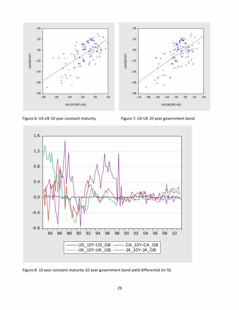
The distinction between the short and long horizon results can be conveyed by comparing

Figures 5 and 6 against Figures 2‐4. Figures 5 and 6 depict, respectively, the 5 and 10 year exchange rate

change‐interest differential relationships. What jumps out is that the regression line slopes are now

positive.

However, the above long horizon results are noticeably less favorable to the unbiasedness

hypothesis than those in Chinn and Meredith (2004). There, none of the estimated coefficients were

negative, and in Chinn and Meredith (2005) the results survived using the Deutschemark as a base

currency. If one focuses on estimates of with U.S. dollar as the base currency, and ignore estimates

based on the pound, our results with the extended sample are much closer to Chinn and Meredith

(2004). Many of the low and negative estimates of in Table 2 involve the Swiss Franc and the Japanese

Yen.

4. Accounting for the Findings

One can identify the sources of the identified pattern. First consider the failure of the hypothesis 1.

This could arise because:

i) Our assumption about rational expectation does not hold and/or our assumption about no

time‐varying risk premium does not hold.

11

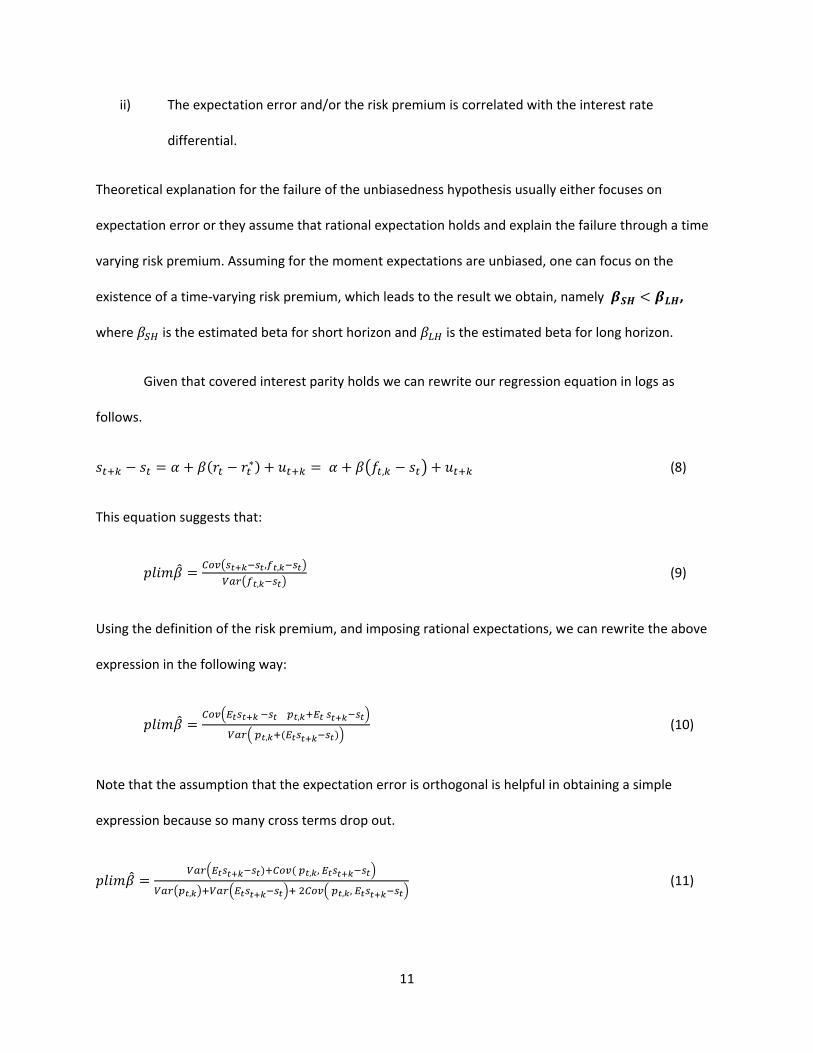
ii) The expectation error and/or the risk premium is correlated with the interest rate

differential.

Theoretical explanation for the failure of the unbiasedness hypothesis usually either focuses on

expectation error or they assume that rational expectation holds and explain the failure through a time

varying risk premium. Assuming for the moment expectations are unbiased, one can focus on the

existence of a time‐varying risk premium, which leads to the result we obtain, namely ,

where is the estimated beta for short horizon and is the estimated beta for long horizon.

Given that covered interest parity holds we can rewrite our regression equation in logs as

follows.

∗ , (8)

This equation suggests that:

, ,

, (9)

Using the definition of the risk premium, and imposing rational expectations, we can rewrite the above

expression in the following way:

,

, (10)

Note that the assumption that the expectation error is orthogonal is helpful in obtaining a simple

expression because so many cross terms drop out.

, ,

, , , (11)

12

The above expression highlights the importance of three components: the variance of the expected

exchange rate depreciation, , the covariance of the of risk premium with the expected

exchange rate depreciation, , , , and the variance of the risk premium, , .

An estimate of 0implies that , , < 0. In a seminal paper, Fama (1984)

demonstrates that, under rational expectations, that , > at short horizons.

Hence, theoretical models that attempt to explain the failure of UIP by assuming rational expectation

and allowing for time varying risk premium, mostly focus on generating the following two conditions:

i) , , 0 and

ii) , , ,

Our empirical finding suggests that in addition to 0, theoretical models also have to explain why

. This implies theoretical models need to incorporate the fact that the building blocks of

might be functions of the horizon k.

We now consider what conditions could generate by focusing on how varies with

each of the three components. Taking the derivative of the expression for the with respect to the

variance of the expected depreciation, one finds that the derivative is positive as long as condition (ii)

holds. Thus if the variance of the expected depreciation increases with the horizon, the will rise

as well. The details of the derivation are contained in Appendix 2.

Although we do not observe , we observe . The variance of

,( ), increases with horizon k, but less than linearly after a certain point.11

However, this pattern for does not necessarily mean of the same pattern holds for

. where is the expectation

11 The variance of changes increases linearly up to a horizon of about four years, but then less rapidly thereafter.

13

error at horizon k from equation 5. Lower values of at longer horizons than implied by a

random walk characterization of the exchange rate might arise because and not

grows less than linearly at longer horizons. Within the rational expectations

framework, not much more can be said.1213

The derivative of with respect to , , is positive as long as condition (ii)

holds14. Thus estimates of will increase with k if the covariance between the risk premium and

expected depreciation also increases with k and condition (ii) holds. This can explain the finding

. In order to explain 0 , models usually incorporate a mechanism whereby , ,

will be negative. In order to explain we need to assume , , will be

less negative or positive as the horizon increases.

Chinn and Meredith (2004) accomplish this by assuming the risk premium term (actually just a

random shock without persistence) exists at the short horizon, in the context of a Keynesian macro

model with Taylor rule reaction functions.15 The implied risk premium at longer horizons is a direct

function of the short horizon risk premium. In the resulting model, the short interest rates are more

endogenous at short horizons than long, motivating the findings.16

12 The expectational error could be relatively smaller because purchasing power parity is expected to hold in the long run, thus anchoring expectations. See Gagnon with Hinterschweiger (2011), Chapter 3. 13 Using survey data on exchange rate expectations from Chinn and Frankel (2002), one finds that the variance of expected depreciation declines with horizon. 14 See Appendix for derivation. 15 This approach is inspired by McCallum’s (1994) model, which incorporates a simpler monetary reaction function. See Engel and West (2006) and Mark (2009). 16 Chinn and Meredith (2005) discuss how long rates appear more weakly exogenous than short rates, in an error correction framework.

14

The relationship of to the , is complicated. At the short horizon, a higher variance

raises the slope coefficient as long as conditions (i) and (ii) hold. However, if condition (ii) holds at long

horizon, higher values , cannot change the sign of from negative to positive.17

There is substantial evidence exchange rate expectations are not unbiased. If one relaxes the

assumption of rational expectations, then the expression for is much more complicated. The

numerator then depends on two additional terms – the covariance between the expectations error and

the risk premium, and the covariance between the expectations error and expected depreciation. This

complicates the determination of how the implied slope coefficient changes with the horizon. In

general, holding the other factors constant, the more positive the covariance terms, the more positive

the . 18

5. Robustness Tests

5.1 Additional Countries

One can expand the set of countries examined (slightly) by using less appropriate data. Thus far, we

have employed constant maturity yields from government bonds, so that the yields correspond to the

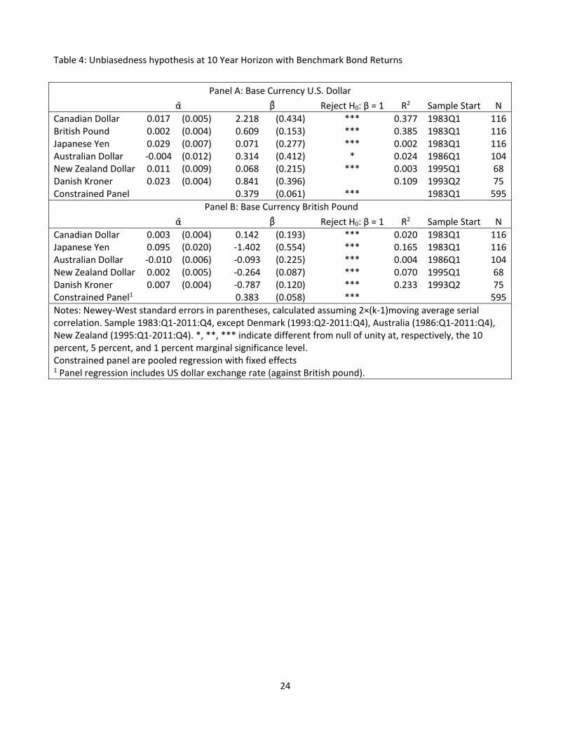
exchange rate horizons. In Table 4, we report estimates using benchmark yields instead of constant

maturity yields. The ten year benchmark yields are yields on government bonds that mature close to ten

years but not in exactly ten years; hence there is some maturity mismatch. The advantage of benchmark

yields is that they are more widely available and do not need to be estimated.

17 We do not account for conditional second moments in the driving processes, such as in Domowitz and Hakkio (1985), or Baillie and Bollerslev (1990). 18 Note that we have only addressed the relations between the interest rate differential and subsequent exchange rate change. In order to deal with the correlation between interest differentials and contemporaneous exchange rate strength, one needs a more complicated framework, as shown in Engel (2011).

15

In addition to long term benchmark yields on government bonds for the U.S., the U.K., Canada

and Japan we use benchmark yields for Australia, New Zealand and Denmark to test the UIP

relationship.19 Figure 7 shows the exchange rate depreciation – interest differential relationship.

In Panel A, we can see that all the estimates of are positive with the U.S. dollar as the base

currency. The estimate of for the Danish Kroner was 0.84, close to the theoretical value. When we

change the base currency to the British Pound, in Panel B, the estimate of becomes negative for all

currency pairs save the Canadian dollar. It is not entirely surprising that the results change, since the two

interest rate series differ. The difference between the constant maturity and benchmark yields is shown

in Figure 8.

The differences are not sufficient to overturn the results entirely, though. The estimate of is

approximately 0.4 in the constrained panel regression in both panels. This point estimate is substantially

closer to 1 than the short horizon estimates, although it is also significantly different from that value.

The fact that the panel slope coefficient is positive, when the individual slope coefficients are negative.

This suggests that the cross sectional variation is often critical in estimating the parameter.

5.2 The Financial Crisis of 2008

Did the 2008 financial crisis affect our results? One of the underlying assumptions in UIP is that

financial markets work efficiently in a way to remove arbitrage conditions. During the 2008 financial

crisis, investors were wary to invest and credit in financial markets dried up. Natural buyers of many

assets remained in the sidelines to allow fire sales. Under these circumstances, covered interest parity

failed to hold as default premia increased (Coffey, Hrung and Sarkar, 2009).

19 The benchmark yield series we collected for Switzerland have less than forty observations at the ten year horizon so we do not include the Swiss Franc in our analysis.

16

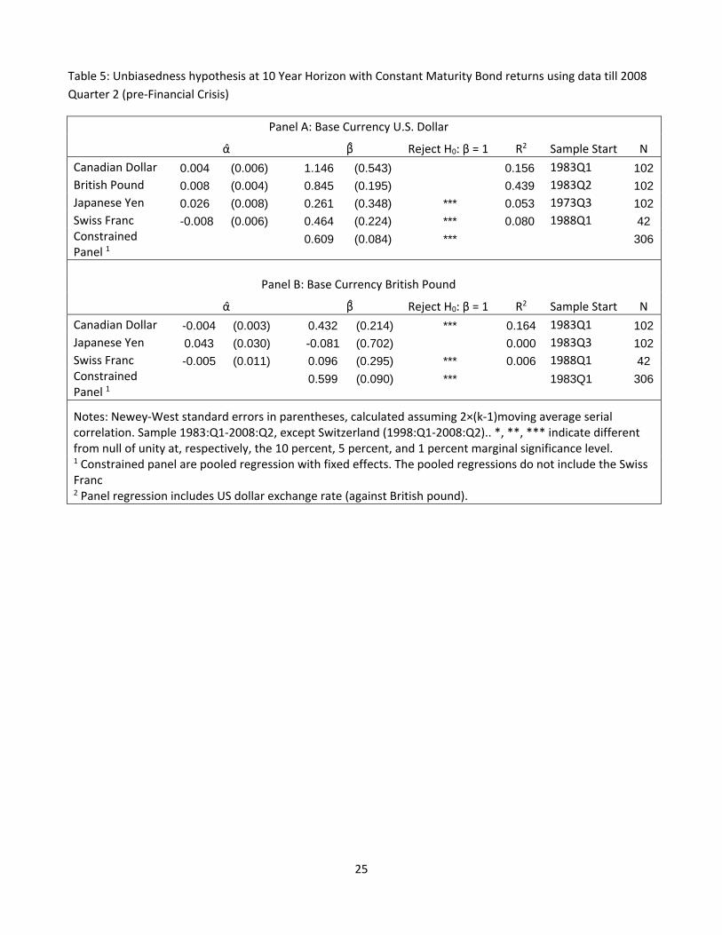
In Table 5, we report estimates from the Fama regression for ten year constant maturity bond

returns, ending the sample at the second quarter 2008. In Panel A, with the U.S. Dollar as the base

currency, we can see that the estimates of are all positive and in two cases we cannot reject the null

hypothesis of 1 for all currencies except the Swiss Franc. The UK regression results in particular are

not markedly different from the corresponding regression results in Table 4. The constrained panel

regression yields an estimate of about 0.6 which is closer to 1 than to zero.

Examining Panel B, the estimate of from the Japanese Yen and British Pound pair is negative,

but the Swiss franc coefficient is positive, in contrast to the estimates based only on pre‐financial crisis

data. The panel coefficient here is around the same magnitude as in Panel A, reinforcing the point that

the cross sectional dimension is important in obtaining precise estimates.

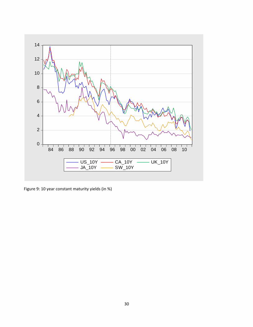
5.3 Low Interest Rate Countries: Japan and Switzerland

Even before the onset of the financial crisis, several countries had short term interest rates near the zero

interest bound. Perhaps more importantly for our results, long term interest rates were particularly

quite low in Japan and Switzerland, two currencies for which the estimated is noticeably low. This

point is illustrated in Figure 9, which shows the time series for 10 year constant maturity yields.

There is no particular reason why the unbiasedness hypothesis should not hold when short

and/or long term rates strike the zero interest bound, as expected exchange rate changes could adjust

to make the parity condition hold. However, it seems worthwhile to investigate the sensitivity of the

estimates to inclusion of the low‐interest rate period. We arbitrarily define 1996Q1 as the low interest

rate period for these two countries, and provide scatterplots in Figures 10‐13, distinguishing between

the two periods. Clearly, the latter period is different.

17

In order to confirm these impressions, we re‐estimate the Fama regression allowing for constant

and slope breaks.

, ,∗

, ,∗ (12)

The dummy variable takes a value of one such that the impact of interest rates in 1996:Q1 on exchange

rate depreciation through 2006:Q1 differs from that in the preceding period.

The results of estimating equation (12) for the yen and Swiss franc are reported in Table 6. They

indicate that post‐1996 the unbiasedness relationship breaks down, with the slope coefficient

significantly different – and negative – in the latter period. The change in the slope coefficient is

statistically significantly different from zero except for the Japanese yen at the 10 year horizon. And in

that case, the slope change is statistically significant in a specification that omits a mean shift.

These findings confirm that the advent of low long term interest rates in Japan and Switzerland

is associated with the attenuation of evidence for the unbiasedness hypothesis at the long horizon – for

currency pairs involving these countries. However, it is not an explanation, as uncovered interest parity

is an arbitrage condition. Our accounting exercise highlights that a changing behavior of the exchange

risk premium, or a changing correlation of expectations errors with the right hand side variables, could

explain the difference in behavior in the latter period.20

6. Conclusion

This paper fills an important gap in the literature regarding long horizon interest rate parity.

When the U.S. Dollar is the base currency, estimates of from long horizon unbiasedness regressions of

five and ten years are usually positive and closer to theoretical value of 1 than their short horizon

counterparts. In many of the cases especially at ten year horizon, we cannot reject the null hypothesis of

20 It could also be the case that the divergent behavior of these two currencies is associated with their large reserve accumulation.

18

1.However, when we extend the analysis to British Pound as the base the currency, we see a

number of estimates of that are negative especially among currency pairs that do not include the U.S.

Dollar. Nonetheless, the panel estimates are uniformly positive. Taken together, we find considerable

evidence of the unbiasedness hypothesis not holding at the long horizon, despite the typically more

positive coefficients. This difference in performance across different currency pairs is consistent with a

time varying risk premium whose properties differ across currency pairs.

The findings are dependent upon the data used and the sample period. In particular, interest

rate data that are not exactly aligned with exchange rate depreciations exhibit less positive results. This

is not particularly surprising.

What is more economically interesting is the fact that the relationship between exchange rate

changes and interest differentials at short horizons has remained unchanged, while it has altered

noticeably in the recent environment of low long term interest rates in certain countries. Since several

other countries have experienced a similar phenomenon of low long term interest rates – including the

US – we should not be surprised if the positive association detected in previous studies is attenuated in

studies that incorporate more recent data.

Our accounting exercise highlights the conditions under which the pattern of results arise,

assuming that expectations errors are random, and uncorrelated with other contemporaneous factors.

However, we also show that if expectations errors are not random, then there are numerous reasons

why the pattern of short and long horizon coefficients arises. We reserve the task of paring down the

number of explanations for future research.

19

References

Alexius, Annika. 2001. “Uncovered Interest Parity Revisited,” Review of International Economics 9(3): 505–17.

Baillie, Richard and Tim Bollerslev, 1990, “A Multivariate Generalized ARCH Approach to Modeling Risk

Premia in Forward Foreign Exchange Rate Markets,” Journal of International Money and Finance 9(3): 309‐324.

Bansal, Ravi, and Magnus Dahlquist, 2000, ‘The forward premium puzzle: different tales from developed and emerging economies,’ Journal of International Economics 51: 115‐144.

Bekaert, Geert, Min Wei and Yuhang Xing, 2007, “Uncovered Interest Rate Parity and the Term Structure,” Journal of International Money and Finance26 (6): 1038‐69.

Chinn, Menzie D., 2012, “(Almost) A Quarter Century of Currency Expectations Data: Interest Rate Parity and the Risk Premium,” mimeo (August).

Chinn, Menzie D., 2006,“The (Partial) Rehabilitation of Interest Rate Parity: Longer Horizons, Alternative

Expectations and Emerging Markets,” Journal of International Money and Finance 25 (1): 7‐21.

Chinn, Menzie D. and Jeffrey A. Frankel, 1994, “Patterns in Exchange Rate Forecasts for 25 Currencies,” Journal of Money, Credit and Banking 26 (4) (November): 759‐770.

Chinn, Menzie, and Guy Meredith. 2004. “Monetary Policy and Long‐Horizon Uncovered Interest Parity.” IMF Staff Papers 51 (3): 409‐30.

Chinn, Menzie D., and Guy Meredith, 2005, “Testing Uncovered Interest Parity at Short and Long

Horizons during the Post‐Bretton Woods Era,” NBER Working Paper No. 11077 (January).

Cochrane, John, 1991, “Production‐Based Asset Pricing and the Link between Stock Returns and Economic Fluctuations,” Journal of Finance 46 (March): 207‐234.

Coffey, Niall, Warren B. Hrung, and Asani Sarkar. 2009. “Capital Constraints, Counterparty Risk, and Deviations from Covered Interest Rate Parity,” Federal Reserve Bank of New York Staff Reports no. 393 (October 2009).

Domowitz, Ian and Craig Hakkio, 1985, “Conditional Variance and the Risk Premium in the Foreign

Exchange Market,” Journal of International Economics 19: 47–66.

Dooley, Michael P., and Peter Isard, 1980, “Capital controls, political risk, and deviations from interest‐rate parity,” Journal of Political Economy 88 (2): 370‐84.

Engel, Charles, 2011, The Real Exchange Rate, Real Interest Rates, and the Risk Premium. Charles Engel. NBER Working Paper No. 17116 (June).

Engel, Charles, 1996, “The Forward Discount Anomaly and the Risk Premium: A Survey of Recent Evidence,” Journal of Empirical Finance 3 (June): 123‐92.

20

Engel, Charles, and Kenneth D. West, 2006, “Taylor Rules and the Deutschmark–Dollar Real Exchange

Rate,” Journal of Money, Credit, and Banking 38(5) (August): 1175‐1194.

Fama, Eugene. 1984. “Forward and Spot Exchange Rate,” Journal of Monetary Economics 14:319‐38.

Flood, Robert P. and Andrew K. Rose, 1996, “Fixes: Of the Forward Discount Puzzle,” Review of

Economics and Statistics: 748‐752.

Flood, Robert B. and Andrew K. Rose, 2002, “Uncovered Interest Parity in Crisis,” International Monetary Fund Staff Papers 49: 252‐66.

Flood, Robert P. and Mark P. Taylor, 1997, “Exchange Rate Economics: What’s Wrong with the Conventional Macro Approach?” in The Microstructure of Foreign Exchange Markets (Chicago: U.Chicago for NBER), pp. 262‐301.

Frankel, Jeffrey A. and Kenneth A. Froot, 1987,"Using Survey Data to Test Standard Propositions Regarding Exchange Rate Expectations," American Economic Review. 77(1) (March): 133‐153.

Frankel, Jeffrey A. and Jumana Poonawala, 2010. "The forward market in emerging currencies: Less biased than in major currencies," Journal of International Money and Finance 29(3): 585‐598.

Froot, Kenneth A. and Jeffrey A. Frankel, 1989,"Forward Discount Bias: Is It an Exchange Risk Premium?" Quarterly Journal of Economics 104(1) (February): 139‐161.

Froot, Kenneth A. and Richard H. Thaler, 1990, “Foreign Exchange,” Journal of Economic Perspectives 4(3) (Summer): 179‐192.

Gagnon, Joseph with Marc Hinterschweiger, 2011, Flexible Exchange Rates for a Stable World Economy (Washington, D.C.: Peterson Institute for International Economics).

Isard, Peter, 1995, Exchange Rate Economics (Cambridge: Cambridge University Press).

McCallum, Bennet T., 1994, “A Reconsideration of the Uncovered Interest Parity Relationship,” Journal

of Monetary Economics 33: 105‐132.

MacDonald, Ronald and Mark P. Taylor, 1992, “Exchange Rate Economics: A Survey,” IMF Staff Papers 39(1): 1‐57.

Madarassy, Rita, and Menzie D. Chinn, 2002, “Free to Flow? New Results on Capital Mobility amongst the Developed Countries,” Santa Cruz Center for International Economics Working Paper No. 02‐20 (May).

Mark, Nelson, 2009, “Changing Monetary Policy Rules, Learning, and Real Exchange Rate Dynamics,” Journal of Money, Credit, and Banking 41(6): 1047‐1070.

Meese, Richard, and Kenneth Rogoff, 1983, "Empirical Exchange Rate Models of the Seventies: Do They

Fit Out of Sample?" Journal of International Economics 14: 3‐24.

Popper, Helen, 1993, “Long‐Term Covered Interest Parity—Evidence From Currency Swaps,” Journal of

International Money and Finance 12(4): 439‐48.

21

Table 1: Unbiasedness hypothesis at the Short Horizon: Estimates of

Base Currency: U.S. Dollar

Currency 3‐Month 6‐Month 12‐Month

Canadian Dollar ‐0.166 (0.713) ‐0.084* (0.700) ‐0.055 (0.705)

British Pound ‐1.847** (0.988) ‐1.554** (0.985) ‐1.006*** (0.905)

Japanese Yen ‐2.478*** (0.733) ‐2.785*** (0.628) ‐2.440*** (0.512)

Swiss Franc ‐2.213* (1.058) ‐2.864*** (1.362) ‐2.779*** (1.138)

Euro ‐2.251 (2.229) ‐1.991 (2.178) ‐2.179 (2.020)

Constrained Panel1 ‐1.241*** (0.558) ‐1.638*** (0.382) ‐1.801*** (0.458)

Base Currency: British Pound

3‐Month 6‐Month 12‐Month

Canadian Dollar ‐3.536*** (1.005) ‐2.503*** (0.964) ‐1.257** (0.876)

Japanese Yen ‐2.101** (1.347) ‐2.006*** (1.043) ‐1.651*** (0.843)

Swiss Franc ‐2.828** (1.476) ‐1.556** (0.978) ‐2.287*** (0.709)

Euro ‐0.299 (1.925) ‐0.081 (1.767) ‐0.662 (1.639)

Constrained Panel1, 2 ‐2.160*** (0.849) ‐1.969*** (0.783) ‐1.401*** (0.703)

Notes: Newey‐West standard error in brackets calculated assuming 2×(k‐1) serial correlation. *, **, *** indicate different from null of unity at, respectively, the 10 percent, 5 percent, and 1 percent marginal significance level. The sample ends in 2011:Q4 for all currencies. Sample begins from 1975:Q1 for all currencies except the Swiss Franc. For the Swiss Franc the 3‐month data begins from 1991:Q2, the 6‐month data begins from 1996:Q4 and the 12‐month data begins from 1997:Q1. Euro data begins 1999Q1. 1 Fixed‐effects regression with standard errors adjusted for serial correlation. The panel regression does not include Swiss Franc, or euro. 2 Panel regression includes US dollar exchange rate (against British pound).

22

Table 2: Unbiasedness hypothesis at Five Year Horizon with Constant Maturity Bond Returns

Panel A: Base Currency U.S. Dollar

α̂ β Reject H0: β = 1 R2 Sample Start N

Canadian Dollar 0.004 (0.007) 0.691 (0.636) 0.027 1978Q1 136

British Pound 0.000 (0.009) 0.415 (0.371) 0.024 1978Q1 136

Japanese Yen 0.031 (0.012) 0.545 (0.374) 0.000 1979Q3 130

Swiss Franc 0.022 (0.013) ‐0.165 (0.519) ** 0.002 1993Q1 76

Constrained Panel1

0.380 (0.186) *** 1978Q1 402

Panel B: Base Currency British Pound


Canadian Dollar ‐0.007 (0.006) ‐0.232 (0.405) *** 0.0007 1978Q1 136

Japanese Yen 0.064 (0.034) ‐0.624 (0.811) ** 0.012 1978Q1 136

Swiss Franc 0.014 (0.022) 0.188 (0.640) 0.002 1993Q1 76

Constrained Panel1,2

0.071 (0.178) *** 1978Q1 402

Notes: Newey‐West standard errors in parentheses, calculated assuming 2×(k‐1)moving average serial correlation. Sample 1978:Q1‐2011:Q4, except for Japan (1979:Q3‐2011:Q4), Switzerland (1993:Q1‐2011:Q4). *, **, *** indicate different from null of unity at, respectively, the 10 percent, 5 percent, and 1 percent marginal significance level. 1. Constrained panels are pooled regression with fixed effects. The pooled regression does not include Swiss Franc. 2 Panel regression includes US dollar exchange rate (against British pound).

23

Table 3: Unbiasedness hypothesis at 10 Year Horizon with Constant Maturity Bond Returns




British Pound 0.006 (0.003) 0.769 (0.177) 0.418 1983Q1 116

Japanese Yen 0.026 (0.008) 0.214 (0.315) *** 0.016 1973Q1 116

Swiss Franc 0.009 (0.013) 0.211 (0.431) ** 0.007 1998Q1 56 Constrained Panel1

0.598 (0.071) *** 1983Q1 348



Canadian Dollar 0.003 (0.004) 0.220 (0.239) *** 0.031 1983Q1 116

Japanese Yen 0.036 (0.025) 0.053 (0.623) 0.000 1983Q1 116

Swiss Franc 0.047 (0.013) ‐1.215 (0.422) *** 0.373 1998Q1 56 Constrained Panel1,2

0.459 (0.099) *** 1983Q1 348

Notes: Newey‐West standard errors in parentheses, calculated assuming 2×(k‐1)moving average serial correlation. Sample 1983:Q1‐2011:Q4, except Switzerland (1998:Q1‐2011:Q4). *, **, *** indicate different from null of unity at, respectively, the 10 percent, 5 percent, and 1 percent marginal significance level. 1Constrained panel are pooled regression with fixed effects. The pooled regression does not include Swiss Franc 2 Panel regression includes US dollar exchange rate (against British pound).

24

Table 4: Unbiasedness hypothesis at 10 Year Horizon with Benchmark Bond Returns



Canadian Dollar 0.017 (0.005) 2.218 (0.434) *** 0.377 1983Q1 116British Pound 0.002 (0.004) 0.609 (0.153) *** 0.385 1983Q1 116Japanese Yen 0.029 (0.007) 0.071 (0.277) *** 0.002 1983Q1 116Australian Dollar ‐0.004 (0.012) 0.314 (0.412) * 0.024 1986Q1 104New Zealand Dollar 0.011 (0.009) 0.068 (0.215) *** 0.003 1995Q1 68 Danish Kroner 0.023 (0.004) 0.841 (0.396) 0.109 1993Q2 75 Constrained Panel 0.379 (0.061) *** 1983Q1 595



Canadian Dollar 0.003 (0.004) 0.142 (0.193) *** 0.020 1983Q1 116Japanese Yen 0.095 (0.020) ‐1.402 (0.554) *** 0.165 1983Q1 116Australian Dollar ‐0.010 (0.006) ‐0.093 (0.225) *** 0.004 1986Q1 104New Zealand Dollar 0.002 (0.005) ‐0.264 (0.087) *** 0.070 1995Q1 68 Danish Kroner 0.007 (0.004) ‐0.787 (0.120) *** 0.233 1993Q2 75 Constrained Panel1 0.383 (0.058) *** 595

Notes: Newey‐West standard errors in parentheses, calculated assuming 2×(k‐1)moving average serial correlation. Sample 1983:Q1‐2011:Q4, except Denmark (1993:Q2‐2011:Q4), Australia (1986:Q1‐2011:Q4), New Zealand (1995:Q1‐2011:Q4). *, **, *** indicate different from null of unity at, respectively, the 10 percent, 5 percent, and 1 percent marginal significance level. Constrained panel are pooled regression with fixed effects 1 Panel regression includes US dollar exchange rate (against British pound).

25

Table 5: Unbiasedness hypothesis at 10 Year Horizon with Constant Maturity Bond returns using data till 2008

Quarter 2 (pre‐Financial Crisis)




British Pound 0.008 (0.004) 0.845 (0.195) 0.439 1983Q2 102

Japanese Yen 0.026 (0.008) 0.261 (0.348) *** 0.053 1973Q3 102

Swiss Franc -0.008 (0.006) 0.464 (0.224) *** 0.080 1988Q1 42 Constrained Panel 1

0.609 (0.084) *** 306



Canadian Dollar -0.004 (0.003) 0.432 (0.214) *** 0.164 1983Q1 102

Japanese Yen 0.043 (0.030) -0.081 (0.702) 0.000 1983Q3 102

Swiss Franc -0.005 (0.011) 0.096 (0.295) *** 0.006 1988Q1 42 Constrained Panel 1

0.599 (0.090) *** 1983Q1 306

Notes: Newey‐West standard errors in parentheses, calculated assuming 2×(k‐1)moving average serial correlation. Sample 1983:Q1‐2008:Q2, except Switzerland (1998:Q1‐2008:Q2).. *, **, *** indicate different from null of unity at, respectively, the 10 percent, 5 percent, and 1 percent marginal significance level. 1 Constrained panel are pooled regression with fixed effects. The pooled regressions do not include the Swiss Franc 2 Panel regression includes US dollar exchange rate (against British pound).

26

Table 6: Allowing for Structural Breaks

Panel A: Five year horizon (k=20)

α̂ β γ θ R2

Japanese yen 0.029*** (0.013) 0.420 (0.415) 0.039 (0.028) ‐1.738*** (0.690) 0.081

Swiss franc ‐0.004 (0.011) 0.251 (0.295) 0.078 (0.018) ‐2.105 (0.887) 0.242

Panel B: Ten year horizon (k=40)

α̂ β γ θ R2

Japanese yen 0.026 (0.008) 0.405 (0.350) 0.002 (0.031) ‐0.646 (0.786) 0.092

Swiss franc ‐0.010* (0.006) 0.356*** (0.162) 0.082*** (0.024) ‐2.093*** (0.969) 0.604

Notes: Newey‐West standard errors in parentheses, calculated assuming 2×(k‐1) moving average serial correlation. Sample Japan (1983:Q1‐2011:Q4), Switzerland (1998:Q1‐2011:Q4). *, **, *** indicate different from null of zero at, respectively, the 10 percent, 5 percent, and 1 percent marginal significance level.

27

Figure 1: Panel beta coefficients at different horizons.

Notes: Up to 12 months, panel estimates for 6 currencies against US$, eurodeposit rates, 1980q1‐00q4; 3 year

results are zero coupon yields, 76q1‐99q2; 5 and 10 years, constant yields to maturity, 80q1‐00q4 and 83q1‐

00q4. Source: Chinn (2006).

-0.8

-0.4

0.0

0.4

0.8

1.2

-0.76 -0.76

-0.54

0.09

0.67 0.68

3 mos. 6 mos . 1 year 3 years 5 years 10 years

/Unbiasednesscoefficient value

28

Figure 2: US‐UK 3 month Figure 3: US‐UK 6 month

Figure 4: US‐UK 1 year Figure 5: US‐UK 5 year constant maturity

-.5

-.4

-.3

-.2

-.1

.0

.1

.2

.3

.4

-.08 -.06 -.04 -.02 .00 .02 .04

UK6MDIF(-2)

UK

DE

P6

M

-.16

-.12

-.08

-.04

.00

.04

.08

-.07 -.06 -.05 -.04 -.03 -.02 -.01 .00 .01 .02

UK5YDIF(-20)

UK

DE

P5Y

-.6

-.4

-.2

.0

.2

.4

.6

.8

-.08 -.06 -.04 -.02 .00 .02 .04 .06

UK3MDIF(-1)

UK

DE

P3

M

-.3

-.2

-.1

.0

.1

.2

.3

-.08 -.06 -.04 -.02 .00 .02 .04

UK1YDIF(-4)

UK

DE

P1

Y

29

Figure 6: US‐UK 10 year constant maturity Figure 7: US‐UK 10 year government bond

Figure 8: 10 year constant maturity‐10 year government bond yield differential (in %)

-.08

-.06

-.04

-.02

.00

.02

.04

-.10 -.08 -.06 -.04 -.02 .00 .02 .04

UKGBDIF(-40)

UK

DE

P10

Y

-0.8

-0.4

0.0

0.4

0.8

1.2

1.6

84 86 88 90 92 94 96 98 00 02 04 06 08 10

US_10Y-US_GB CA_10Y-CA_GBUK_10Y-UK_GB JA_10Y-JA_GB

-.08

-.06

-.04

-.02

.00

.02

.04

-.08 -.06 -.04 -.02 .00 .02

UK10YDIF(-40)

UK

DE

P10

Y

30

Figure 9: 10 year constant maturity yields (in %)

0

2

4

6

8

10

12

14

84 86 88 90 92 94 96 98 00 02 04 06 08 10

US_10Y CA_10Y UK_10YJA_10Y SW_10Y

31

-.04

-.02

.00

.02

.04

.06

.08

.10

.12

-.02 -.01 .00 .01 .02 .03 .04 .05 .06 .07

JA10YDIF(-40)

JAD

EP

10Y

Figure 10: US‐Japan 5 year constant maturity Figure 11: US‐Swiss 5 year government bond

Blue: post‐1996 interest rates Blue: post‐1996 interest rates

Figure 12: US‐Japan 10 year constant maturity Figure 13: US‐Swiss 10 year government bond

Blue: post‐1996 interest rates Blue: post‐1996 interest rates

-.10

-.05

.00

.05

.10

.15

.20

-.02 -.01 .00 .01 .02 .03 .04 .05

SW5YDIF(-20)

SW

DE

P5Y

-.04

-.02

.00

.02

.04

.06

.08

.10

.00 .01 .02 .03 .04 .05

SW10YDIF(-40)

SW

DE

P10

Y

-.08

-.04

.00

.04

.08

.12

.16

-.04 -.02 .00 .02 .04 .06 .08

JA5YDIF(-20)

JAD

EP

5Y

32

Appendix 1. Data Sources

Source Link

U.S. Constant Maturity Bond Yields

Federal Reserve Board of Governors

Downloaded from Bloomberg

U.K. Constant Maturity Bond Yields

Bank of England, Chinn and Meredith (2004)

http://www.bankofengland.co.uk/boeapps/iadb/Index.asp? first=yes&SectionRequired=I&HideNums=‐1&ExtraInfo=true&Travel=NIx

Canadian Constant Maturity Bond Yields

Bank of Canada, Chinn and Meredith (2004)

http://www.bankofcanada.ca/rates/interest‐rates/bond‐yield‐curves/

Swiss Constant Maturity Bond Yields (Yields on Swiss Confederation Bond)

Historical Time Series Data, Swiss National Bank

http://www.snb.ch/en/iabout/stat/statpub/histz/id/statpub_histz_actual

Japanese Constant Maturity Bond Yields

Japanese Ministry of Finance and Chinn and Meredith (2004)

http://www.mof.go.jp/english/jgbs/reference/interest_rate/index.htm

33

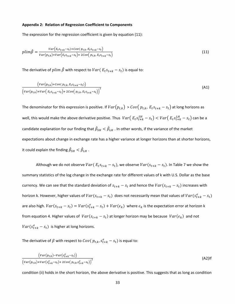
Appendix 2: Relation of Regression Coefficient to Components

The expression for the regression coefficient is given by equation (11):

, ,

, , , (11)

The derivative of with respect to is equal to:

, , ,

, , , (A1)

The denominator for this expression is positive. If , > , , at long horizons as

well, this would make the above derivative positive. Thus can be a

candidate explanation for our finding that . In other words, if the variance of the market

expectations about change in exchange rate has a higher variance at longer horizons than at shorter horizons,

it could explain the finding .

Although we do not observe , we observe . In Table 7 we show the

summary statistics of the log change in the exchange rate for different values of k with U.S. Dollar as the base

currency. We can see that the standard deviation of and hence the increases with

horizon k. However, higher values of does not necessarily mean that values of

are also high. where is the expectation error at horizon k

from equation 4. Higher values of at longer horizon may be because and not

is higher at long horizons.

The derivative of with respect to , , is equal to:

,

, , , (A2)If

condition (ii) holds in the short horizon, the above derivative is positive. This suggests that as long as condition

34

(ii) holds, if the value of covariance between the risk premium and expected change in the exchange rate

increases with k, this can explain our finding . In order to explain 0 models usually have a

mechanism whereby , , will be negative. In order to explain the models can have

a mechanism whereby , , will be less negative or positive as the horizon increases.

The derivative of with respect to , is equal to:

, ,

, , , (A3)

In the short run, if conditions (i) and (ii) holds, then the above derivative is positive. This would be imply,

higher variance of the risk premium at longer horizons can increase the value of at longer horizon. However,

if condition (ii) holds at long horizon, higher values , cannot change the sign of from negative to

positive.

Long Horizon Uncovered Interest Parity Re Assessed · Long Horizon Uncovered Interest Parity Re ......

Documents

Transcript of Long Horizon Uncovered Interest Parity Re Assessed · Long Horizon Uncovered Interest Parity Re ......