Reflector 8.1 User Guide - California Institute of...

Reflector 8.1User Guide

Copyright © 2016, All rights reserved.

Table of Contents

Preface....................................................................................................................................1Conventions Used in This Guide........................................................................................1Where to Find Information..................................................................................................1Technical Support...............................................................................................................2Feedback............................................................................................................................2

Chapter 1 – Introducing Reflector Interface............................................................................3Title Bar...............................................................................................................................4Menu Bar............................................................................................................................4

File Menu........................................................................................................................5Edit Menu.......................................................................................................................6Filter Menu......................................................................................................................6Decon Menu...................................................................................................................7VelAnalysis Menu...........................................................................................................7NMO Menu.....................................................................................................................8Statics Menu...................................................................................................................8Stack Menu.....................................................................................................................8Migration Menu...............................................................................................................9Section Menu.................................................................................................................9Display Menu..................................................................................................................9Window Menu...............................................................................................................10Help Menu....................................................................................................................10

Toolbar..............................................................................................................................10Display Window................................................................................................................11Status Bar.........................................................................................................................11

Chapter 2 – Loading Seismic Data.......................................................................................12Importing Seismic Data....................................................................................................13Loading Seismic Data.......................................................................................................17Saving Seismic Data........................................................................................................17Reviewing Geometry........................................................................................................18Displaying Seismic Data...................................................................................................19

Chapter 3 – Sorting Gathers.................................................................................................20Sorting Gathers.................................................................................................................21Saving a Single Gather.....................................................................................................23

Chapter 4 – Editing Seismic Data.........................................................................................24Divergence Correction......................................................................................................25Gain Control......................................................................................................................26Trace Editing.....................................................................................................................27Trigger Delay Correction..................................................................................................30

Reflector 8.1 User Guide i

Chapter 5 – Filtering Seismic Data.......................................................................................31Frequency Filter................................................................................................................32Time Variant Bandpass Filter...........................................................................................34F-K Filter...........................................................................................................................37Tau-p Filter........................................................................................................................39Random Noise Attenuation...............................................................................................41Frequency Scan...............................................................................................................42

Chapter 6 – Improving S/N Ratio with Deconvolution..........................................................43Spiking Deconvolution......................................................................................................44Predictive Deconvolution..................................................................................................46

Chapter 7 – Analyzing Velocities..........................................................................................48Semblance Spectra..........................................................................................................49Velocity Scan....................................................................................................................54Velocity Evaluation...........................................................................................................57

Chapter 8 – Applying Static Correction.................................................................................58Field Static Correction......................................................................................................59

Elevation Statics...........................................................................................................59Tomo Statics.................................................................................................................61

Residual Static Correction................................................................................................62

Chapter 9 – Creating Stacks.................................................................................................64Time Stack........................................................................................................................65Post-stack Time Migration................................................................................................67Depth Stack......................................................................................................................68Instantaneous Attributes...................................................................................................69Velocity Overlay................................................................................................................70

Chapter 10 – Creating a Processing Log.............................................................................72

Chapter 11 – Outputting Results...........................................................................................73

Reflector 8.1 User Guide ii

Preface

Thank you for choosing Reflector – the Seismic Reflection Data Processing Software in Geogiga Seismic Pro. Using Reflector, you can:

➢ Correct trigger delay.

➢ Sort gathers in the order of common midpoint, common offset, common shot, or common receiver.

➢ Apply field static and residual static correction.

➢ Scale seismic data with divergence correction, gain control, and muting.

➢ Filter seismic data with frequency filter, time variant filter, F-K transform, Tau-P mapping,and random noise attenuation.

➢ Improve the S/N ratio with spiking and predictive deconvolution.

➢ Analyze velocities based on semblance spectra and velocity scan.

➢ Run NMO and inverse NMO correction.

➢ Build time and depth stack.

➢ Migrate stacks.

Conventions Used in This Guide

The conventions used in this guide are given below:

➢ Bold – Represents keystrokes, menu items, window names, or fields.

➢ Italic – Uses for file names, directory names, and emphasis as well.

➢ Courier – Denotes the text to enter.

Where to Find Information

The following list explains what you can find in this guide:

➢ Chapter 1 introduces the Reflector interface.

➢ Chapter 2 describes how to import, display, and save seismic data.

➢ Chapter 3 talks about the gather sorting.

➢ Chapter 4 provides the details on editing seismic data.

➢ Chapter 5 talks about how to filter seismic data.

➢ Chapter 6 discusses the spiking and predictive deconvolution.

➢ Chapter 7 shows how to analyze velocities and evaluate velocity analysis.

➢ Chapter 8 demonstrates the field static and residual static correction.

➢ Chapter 9 explains how to build stacks, create instantaneous attributes, run post-stack migration, and overlay a stack with velocities.

➢ Chapter 10 describes how to create a processing log.

➢ Chapter 11 mentions how to output results.

If you are a first-time user, first read the Getting Started with Geogiga Seismic Pro which can be accessed by clicking the Getting Started command under the Help menu in the Geogiga Seismic Pro Launchpad.

Technical Support

If you have questions, need additional assistance, or encounter a problem, please contact Technical Support using the information given below:

Telephone: 1-403-451 4886

Email: [email protected]

Web: www.geogiga.com

Feedback

To help us improve the future documentation, we want to know any corrections, clarification orfurther information you would find useful. When you contact us, please include the following information:

➢ The title of the documentation you are referring to

➢ The version of the application you are using

➢ Your name, company name, phone number, and email address

Please send us your comments at [email protected].

Preface 2

mailto:[email protected]

mailto:[email protected]

http://www.geogiga.com/

Chapter 1 – Introducing Reflector Interface

The Reflector interface has five parts as shown in figure 1-1:

➢ Title Bar

➢ Menu Bar

➢ Toolbar

➢ Display Window

➢ Status Bar

The following will explain these parts in detail.

Figure 1-1: The Reflector interface

Chapter 1 – Introducing Reflector Interface 3

Title BarMenu Bar

Toolbar

Display Window

Status Bar

Title Bar

The Title Bar shows the seismic data filename.

Menu Bar

The Menu Bar has following menus:

➢ File Menu

➢ Edit Menu

➢ Filter Menu

➢ Decon Menu

➢ VelAnalysis Menu

➢ NMO Menu

➢ Statics Menu

➢ Stack Menu

➢ Migration Menu

➢ Section Menu

➢ Display Menu

➢ Window Menu

➢ Help Menu

When you click one of the menu names, a drop-down submenu appears and displays a list of related commands.


File Menu

The submenu under the File menu, as shown in figure 1-2, contains the commands given below:

➢ Open Seismic – Load seismic data.

➢ Import Seismic – Assign geometry in multiple files (one file per shot) and integrate these shot files.

➢ Save Seismic – Save seismic data.

➢ Save Seismic As – Save seismic data with a new file name.

➢ Open Velocity – Load velocities from a text file.

➢ Save Velocity – Save velocities.

➢ Save Velocity As – Save velocities with a new file name.

➢ Gather Sorting – Sort gathers in the order of commonmidpoint, common offset, common shot, or common receiver.

➢ Save Single Gather – Save a single gather in a file.

➢ Logging – Create a processing log.

➢ Geometry QC – Review and modify geometry.

➢ Print Seismic – Print seismic data with a defined size.

➢ Print Screen – Print an image shown on screen.

➢ Save Image – Save an image shown on screen.

➢ Close – Close seismic data and velocity files.

➢ Exit – Exit Reflector. Figure 1-2: The File submenu


Edit Menu

The submenu under the Edit menu, as shown in figure 1-3, contains the commands listed as follows:

➢ Undo – Erase changes done to seismic data.

➢ Redo – Reverse the Undo.

➢ Gain – Apply gain control on seismic data. The types of gain control include AGC, trace balance, and time variant scaling.

➢ Trace Edit – Mute and scale seismic data in an arbitrary region.

➢ Trigger Delay Correction – Correct trigger delay.

➢ Divergence Correction – Compensate the data amplitude with divergence correction.

Figure 1-3: The Edit submenu

Filter Menu

The submenu under the Filter menu, as shown in figure 1-4, contains the commands givenbelow:

➢ Frequency Filter – Filter seismic data with Butterworth or Ormsby filter.

➢ Time Variant – Filter seismic data with time variant band-pass filter.

➢ Frequency Scan – Scan seismic data in different frequency ranges.

➢ F-K – Filter seismic data in F-K domain.

➢ Tau-p – Filter seismic data in Tau-p domain.

➢ Random Noise – Attenuate random noise.

Figure 1-4: The Filter submenu


Decon Menu

The submenu under the Decon menu, as shown in figure 1-5, contains commands listed as follows:

➢ Spiking – Spiking deconvolution.

➢ Predictive – Predictive deconvolution.

Figure 1-5: The Decon submenu

VelAnalysis Menu

The submenu under the VelAnalysis menu, as shown in figure 1-6, contains commands given below:

➢ Semblance Spectra – Analyze velocities with semblance spectra.

➢ Velocity Scan – Analyze velocities with velocity scan.

➢ Location Selection – Select a location for the velocity analysis.

➢ Build Composite Stack – Update stack with picked velocities.

➢ Delete Velocity Function – Delete velocities at the current location.

➢ Copy Velocity Function – Copy velocities at the current location.

➢ Paste Velocity Function – Paste velocities at the current location.

Figure 1-6: The VelAnalysis submenu


NMO Menu

The submenu under the NMO menu as shown in figure 1-7 contains following commands:

➢ NMO Correction – NMO correction.

➢ Inverse NMO Correction– Inverse NMO correction.

Figure 1-7: The NMO submenu

Statics Menu

The submenu under the Statics menu, as shown in figure 1-8, contains commands listed as follows:

➢ Field Statics – Field static correction.

➢ Residual Statics – Residual static correction.

Figure 1-8: The Statics submenu

Stack Menu

The submenu under the Stack menu as shown in figure 1-9 contains following commands:

➢ Stack – Build time stack.

➢ Save Time Stack – Save time stack in a file.

➢ Time to Depth – Convert time stack to depth stack.

➢ Save Depth Stack – Save depth stack in a file.

➢ Create Attributes – Create instantaneous attributes.

Figure 1-9: The Stack submenu


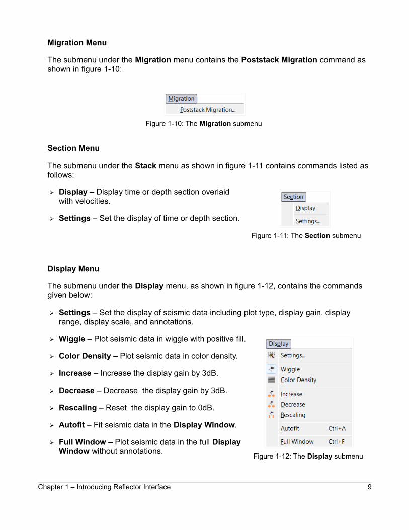
Migration Menu

The submenu under the Migration menu contains the Poststack Migration command as shown in figure 1-10:

Figure 1-10: The Migration submenu

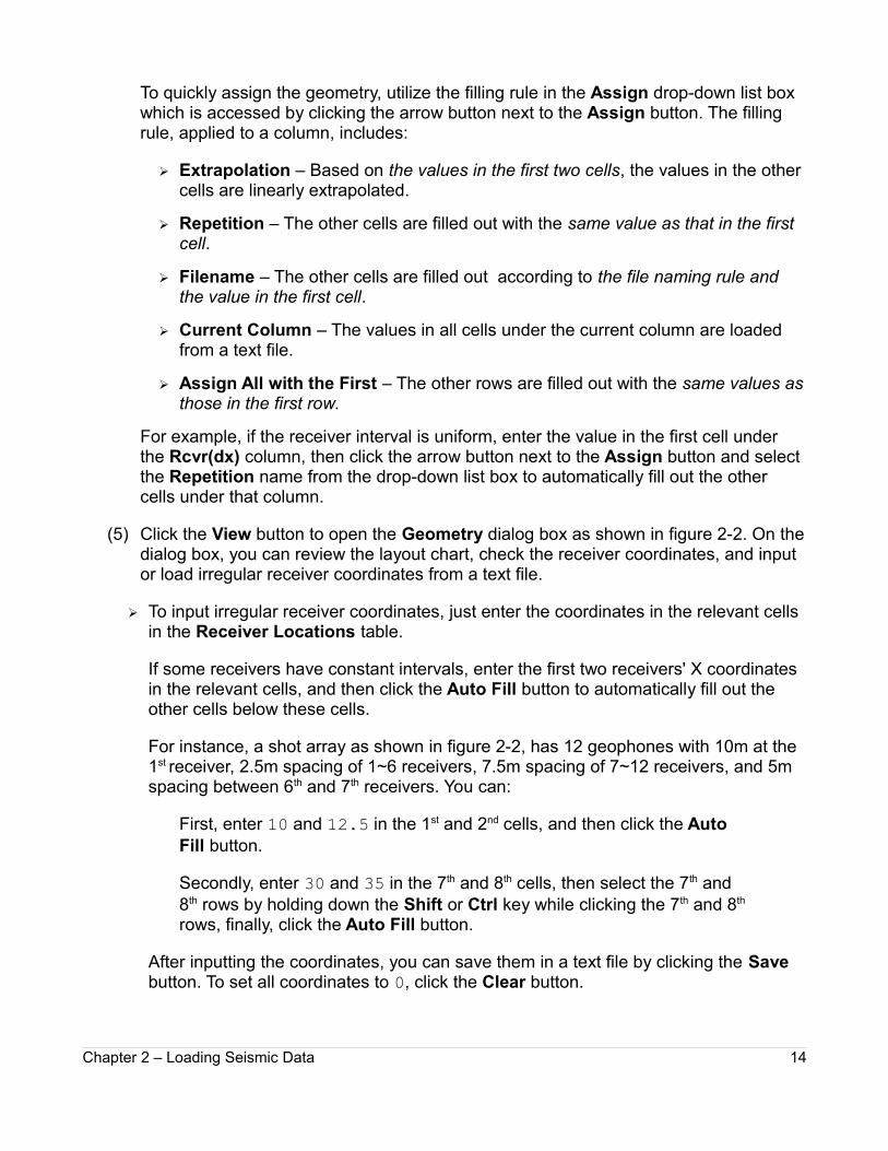
Section Menu

The submenu under the Stack menu as shown in figure 1-11 contains commands listed as follows:

➢ Display – Display time or depth section overlaid with velocities.

➢ Settings – Set the display of time or depth section.

Figure 1-11: The Section submenu

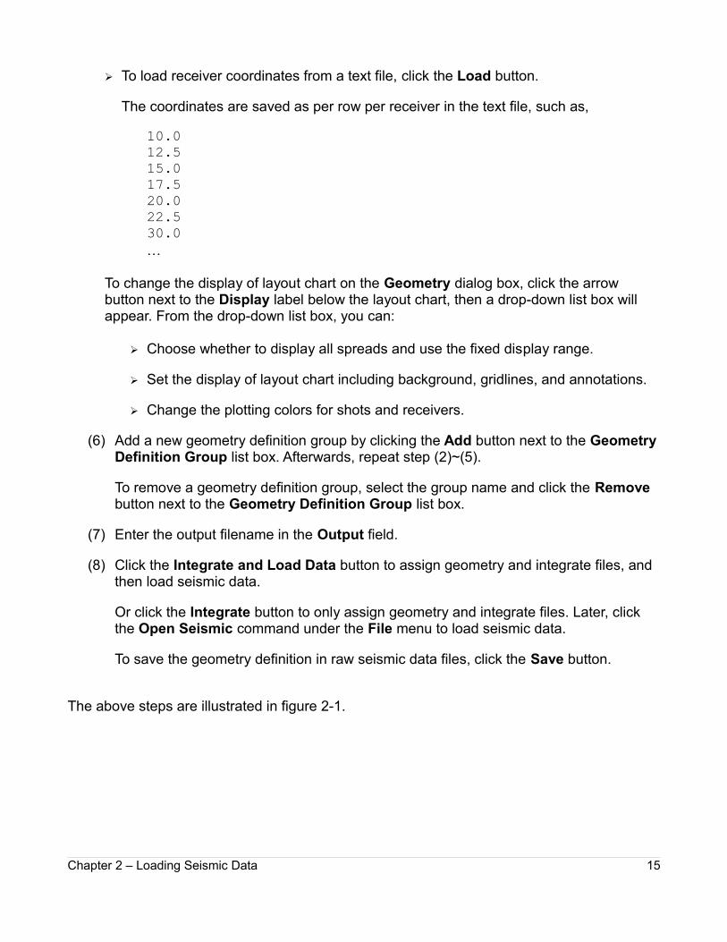
Display Menu

The submenu under the Display menu, as shown in figure 1-12, contains the commands given below:

➢ Settings – Set the display of seismic data including plot type, display gain, display range, display scale, and annotations.

➢ Wiggle – Plot seismic data in wiggle with positive fill.

➢ Color Density – Plot seismic data in color density.

➢ Increase – Increase the display gain by 3dB.

➢ Decrease – Decrease the display gain by 3dB.

➢ Rescaling – Reset the display gain to 0dB.

➢ Autofit – Fit seismic data in the Display Window.

➢ Full Window – Plot seismic data in the full Display Window without annotations.

Figure 1-12: The Display submenu


Window Menu

The submenu under the Window menu, as shown in figure 1-13, contains the following commands:

➢ Toolbars – Toggle the visibility of the Toolbar.

➢ Statusbar – Change the visibility of the Status Bar.

Figure 1-13: The Window submenu

Help Menu

The submenu under the Help menu as shown in figure 1-14 contains following commands:

➢ Manual – Open the User Guide.

➢ About – View information related to Reflector and the computer system memory.

Figure 1-14: The Help submenu

Toolbar

As shown in figure 1-15, the button icons on the Toolbar correspond to the commonly used commands under the menus. To run a command, click its related button icon.

Figure 1-15: Icons on the Toolbar


Display Window

The Display Window varies depending on the operating status. For example, in the velocity analysis, the window displays velocity curve, semblance spectra, CMP gathers, NMO CMP gathers, and time stack overlaid with velocities as shown in figure 1-16.

To adjust the size of any sub windows, drag the separator bar as shown in figure 1-16.

Figure 1-16. The Display Window in velocity analysis

Status Bar

On the Status Bar, you will see the information related to commands and data when moving the mouse cursor over the interface.


Chapter 2 – Loading Seismic Data

This chapter covers the following topics:

➢ Importing seismic data

➢ Loading seismic data

➢ Saving seismic data

➢ Reviewing geometry

➢ Displaying seismic data

Chapter 2 – Loading Seismic Data 12

Importing Seismic Data

If the multiple shot data are saved as per shot per file, you need to import seismic data first.

The purpose of importing seismic data is to:

➢ Assign geometry in multiple files (one file per shot).

➢ Integrate multiple files after geometry assignment.

To import seismic data, open the Geometry Assignment and Files Integration dialog box byclicking the Import Seismic command under the File menu. On the dialog box as shown in figure 2-1:

(1) Select the Group 1 name from the Geometry Definition Group list box.

The group concept is designed to make geometry assignment quicker and easier. Normally, a group should have similar features in order to use the filling rule describedin the step (4).

(2) Enter numbers in the Auxiliary Traces field, such as 1, 2, 6-9.

Leave the field blank if there are no auxiliary or dummy traces in each shot record.

(3) Add multiple files to the Files table by clicking the Add button under the Files table.

(4) Input the relevant geometry information for each shot under the following columns in the Files table.

➢ Shot No. – the shot number which can be any unique number.

➢ Shot(x) – the shot X coordinate.

➢ Shot Depth – the shot depth.

➢ 1st Rcvr No. – the 1st receiver station number used for CMP numbering. This value must be even number.

➢ 1st Rcvr(x) – the1st receiver X coordinate.

➢ Rcvr(dx) – the receiver interval in X direction.


To quickly assign the geometry, utilize the filling rule in the Assign drop-down list box which is accessed by clicking the arrow button next to the Assign button. The filling rule, applied to a column, includes:

➢ Extrapolation – Based on the values in the first two cells, the values in the other cells are linearly extrapolated.

➢ Repetition – The other cells are filled out with the same value as that in the first cell.

➢ Filename – The other cells are filled out according to the file naming rule and the value in the first cell.

➢ Current Column – The values in all cells under the current column are loaded from a text file.

➢ Assign All with the First – The other rows are filled out with the same values asthose in the first row.

For example, if the receiver interval is uniform, enter the value in the first cell under the Rcvr(dx) column, then click the arrow button next to the Assign button and select the Repetition name from the drop-down list box to automatically fill out the other cells under that column.

(5) Click the View button to open the Geometry dialog box as shown in figure 2-2. On thedialog box, you can review the layout chart, check the receiver coordinates, and input or load irregular receiver coordinates from a text file.

➢ To input irregular receiver coordinates, just enter the coordinates in the relevant cells in the Receiver Locations table.

If some receivers have constant intervals, enter the first two receivers' X coordinates in the relevant cells, and then click the Auto Fill button to automatically fill out the other cells below these cells.

For instance, a shot array as shown in figure 2-2, has 12 geophones with 10m at the 1st receiver, 2.5m spacing of 1~6 receivers, 7.5m spacing of 7~12 receivers, and 5m spacing between 6th and 7th receivers. You can:

First, enter 10 and 12.5 in the 1st and 2nd cells, and then click the Auto Fill button.

Secondly, enter 30 and 35 in the 7th and 8th cells, then select the 7th and 8th rows by holding down the Shift or Ctrl key while clicking the 7th and 8th

rows, finally, click the Auto Fill button.

After inputting the coordinates, you can save them in a text file by clicking the Save button. To set all coordinates to 0, click the Clear button.


➢ To load receiver coordinates from a text file, click the Load button.

The coordinates are saved as per row per receiver in the text file, such as,

10.012.515.017.520.022.530.0…

To change the display of layout chart on the Geometry dialog box, click the arrow button next to the Display label below the layout chart, then a drop-down list box will appear. From the drop-down list box, you can:

➢ Choose whether to display all spreads and use the fixed display range.

➢ Set the display of layout chart including background, gridlines, and annotations.

➢ Change the plotting colors for shots and receivers.

(6) Add a new geometry definition group by clicking the Add button next to the GeometryDefinition Group list box. Afterwards, repeat step (2)~(5).

To remove a geometry definition group, select the group name and click the Remove button next to the Geometry Definition Group list box.

(7) Enter the output filename in the Output field.

(8) Click the Integrate and Load Data button to assign geometry and integrate files, and then load seismic data.

Or click the Integrate button to only assign geometry and integrate files. Later, click the Open Seismic command under the File menu to load seismic data.

To save the geometry definition in raw seismic data files, click the Save button.

The above steps are illustrated in figure 2-1.


Figure 2-1: The Geometry Assignment and Files Integration dialog box

Figure 2-2: Inputting irregular receiver coordinates in step (5)


Loading Seismic Data

To load seismic data, click the Open Seismic command under the File menu to launch the Open Seismic File dialog box. On the dialog box as shown in figure 2-3, select a seismic data file, and then click the Open button.

Figure 2-3: The Open Seismic File dialog box

Saving Seismic Data

After changing the geometry or processing seismic data, save the data by clicking the Save Seismic or Save Seismic As command under the File menu.


Reviewing Geometry

To review the geometry after loading seismic data, click the Geometry QC command under the File menu to open the Geometry dialog box as shown in figure 2-4, where you can check and modify the geometry.

To check the geometry, choose a shot record by clicking the left mouse button in the Display Window, then you will see the layout chart and the coordinates are accordingly updated.

There are two ways to modify the geometry: Input or load from a text file. For details on how to input or load coordinates, refer to Step (5) in Importing Seismic Data described earlier.

After changing the geometry, click the Apply button to overwrite the coordinates in the file header for the chosen shot record.

If you want to set the current geometry for all shot records, click the Apply All button.

To save the geometry changes in the seismic file, click the Save Seismic or Save Seismic As command under the File menu.

Figure 2-4: The Geometry dialog box


Displaying Seismic Data

To set the display of seismic data, open the Trace Display dialog box by clicking the Settingscommand under the Display menu. On the dialog box as shown in figure 2-5, you can:

➢ Choose the plot type and adjust the display gain.

➢ Specify the display range of seismic data and view the sample rate.

➢ Define the scale factors.

➢ Change the annotation settings.

➢ Select to plot the trace graph.

To learn about this dialog box, read Chapter 4 in Getting Started with Geogiga Seismic Pro.

For your convenience, the most commonly used commands in the display of seismic data are added to the submenu under the Display menu as shown in figure 1-12.

Figure 2-5: The Trace Display dialog box


Chapter 3 – Sorting Gathers

This chapter covers the following topics:

➢ Sorting gathers

➢ Saving a single gather

Chapter 3 – Sorting Gathers 20

Sorting Gathers

The gathers can be sorted in the order of:

➢ Common Midpoint (CMP)

➢ Common Shot (CSP)

➢ Common Offset

➢ Common Receiver

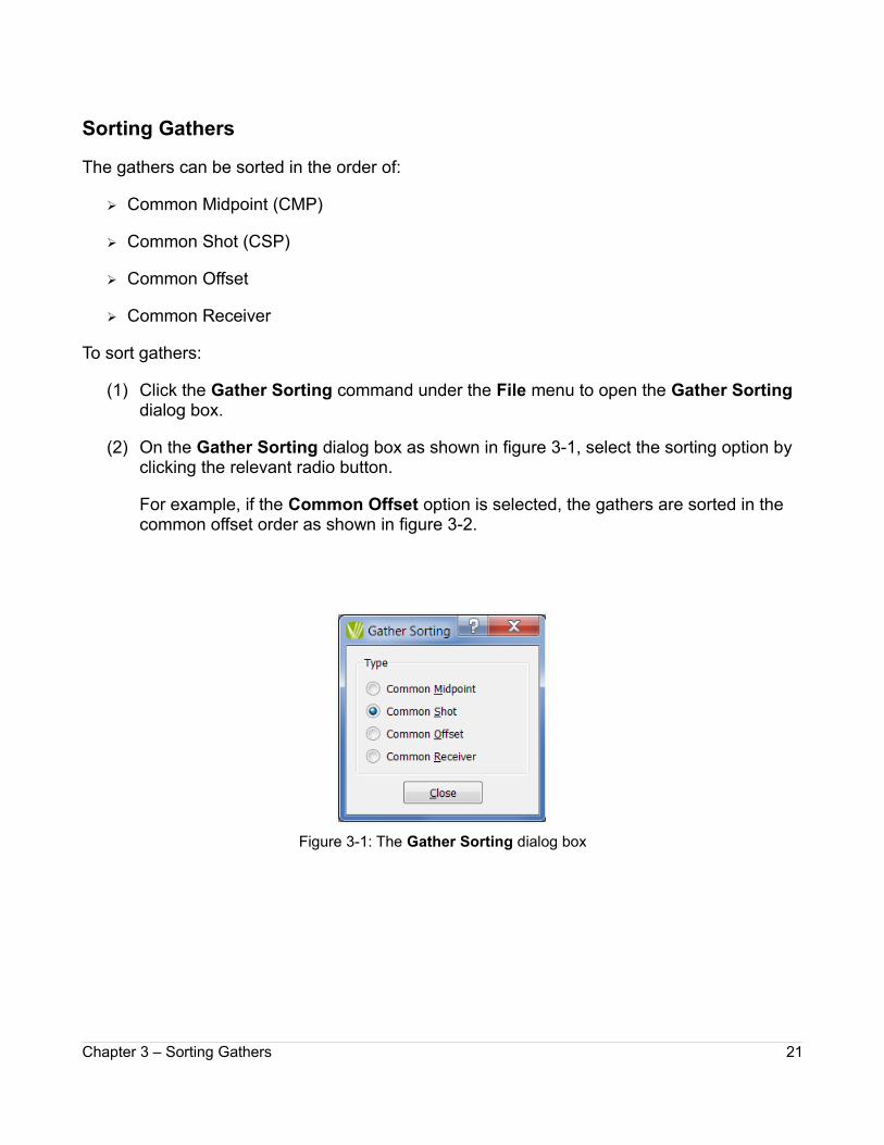
To sort gathers:

(1) Click the Gather Sorting command under the File menu to open the Gather Sorting dialog box.

(2) On the Gather Sorting dialog box as shown in figure 3-1, select the sorting option by clicking the relevant radio button.

For example, if the Common Offset option is selected, the gathers are sorted in the common offset order as shown in figure 3-2.

Figure 3-1: The Gather Sorting dialog box


Figure 3-2: Sorting gathers in the order of common offset

For your convenience, the Gather Sorting command is put on the Toolbar. You can select the sorting option by clicking the arrow button next to the sorting button icon as shown in figure 3-3.

Figure 3-3: The Gather Sorting command on the Toolbar


Saving a Single Gather

To save a single gather after sorting gathers in a specified order:

(1) Click the Save Single Gather command under the File menu to open the Save Gather dialog box.

(2) On the Save Gather dialog box as shown in figure 3-4, select a number from the list box and then click the Save button.

To save all single gathers, select the All option.

The list content will be different, depending on the sorting order.

Figure 3-4 The Save Single Gather dialog box

Normally, the single gather can be loaded in another application of Geogiga Seismic Pro for further processing. For example, SF Imager can handle the common offset gather saved in Reflector.


Chapter 4 – Editing Seismic Data

This chapter talks about how to edit seismic data with:

➢ Divergence correction

➢ Gain control

➢ Trace editing

➢ Trigger delay correction

Chapter 4 – Editing Seismic Data 24

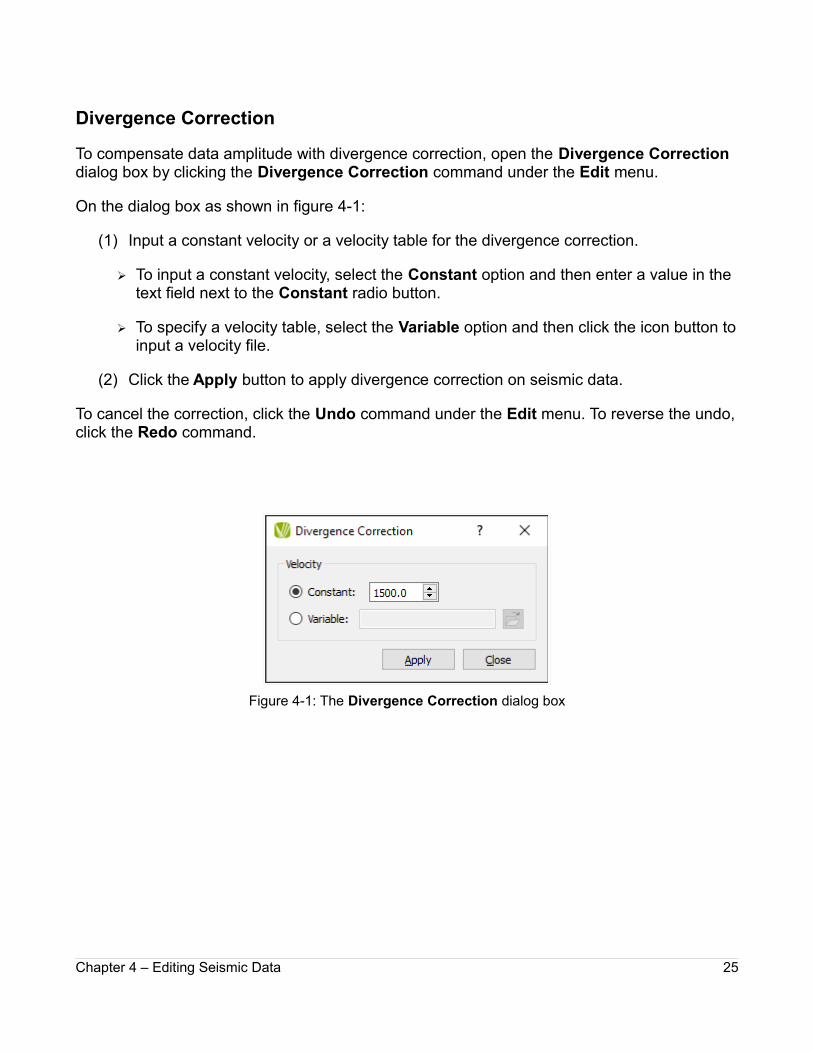
Divergence Correction

To compensate data amplitude with divergence correction, open the Divergence Correction dialog box by clicking the Divergence Correction command under the Edit menu.

On the dialog box as shown in figure 4-1:

(1) Input a constant velocity or a velocity table for the divergence correction.

➢ To input a constant velocity, select the Constant option and then enter a value in the text field next to the Constant radio button.

➢ To specify a velocity table, select the Variable option and then click the icon button toinput a velocity file.

(2) Click the Apply button to apply divergence correction on seismic data.

To cancel the correction, click the Undo command under the Edit menu. To reverse the undo,click the Redo command.

Figure 4-1: The Divergence Correction dialog box


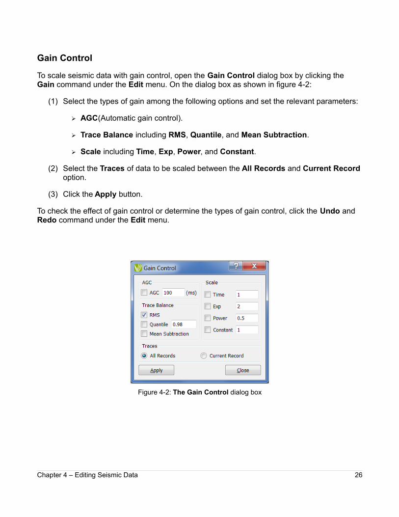
Gain Control

To scale seismic data with gain control, open the Gain Control dialog box by clicking the Gain command under the Edit menu. On the dialog box as shown in figure 4-2:

(1) Select the types of gain among the following options and set the relevant parameters:

➢ AGC(Automatic gain control).

➢ Trace Balance including RMS, Quantile, and Mean Subtraction.

➢ Scale including Time, Exp, Power, and Constant.

(2) Select the Traces of data to be scaled between the All Records and Current Record option.

(3) Click the Apply button.

To check the effect of gain control or determine the types of gain control, click the Undo and Redo command under the Edit menu.

Figure 4-2: The Gain Control dialog box


Trace Editing

To edit seismic data, open the Trace Edit dialog box as shown in figure 4-3 by clicking the Trace Edit command under the Edit menu.

Figure 4-3: The Trace Edit dialog box

On the Trace Edit dialog box:

(1) Select the editing Region among the Above, Below, Inside, Outside, and Single Trace options.

If the Single Trace option is chosen, go to step (5); otherwise, go to step (2).

(2) Click the Add button and then define an editing region on seismic data in the Display Window as shown in figure 4-4.

To insert a control point, click the left mouse button.

To adjust a control point, move the mouse cursor over the point and then drag it.

To delete a control point, move the mouser cursor over the point and then click the right mouse button.


(3) Repeat step (2) to define multiple editing regions.

To cancel an editing region, select the region on seismic data in the Display Window and then click the Remove Current button. To cancel all editing regions, click the Remove All button.

To save the editing regions in a file, click the Save button. This file can be loaded later by clicking the Load button.

(4) Interpolate the editing regions if required, and then go to step (6).

To interpolate editing regions on all records, select the Interpolate option and then click the Interpolate button.

(5) Select a single trace by clicking the left mouse button on seismic data in the Display Window. Afterwards, a mask is plotted on the trace as shown in figure 4-5.

To adjust the time range, drag the top and bottom horizontal blue line.

(6) Increase, decrease, mute, average, or reverse the data amplitude by clicking the >>, <<, 0, 1/2 , or +/- button.

The 1/2 and +/- buttons are enabled only if the Single Trace option is selected.

You can specify the Scaling Factor and Taper in the relevant fields when increasing or decreasing the data amplitude.

To cancel the editing operations, click the Undo command under the Edit menu. To reverse the undo, click the Redo command.


Figure 4-4: Defining the editing region

Figure 4-5: Selecting a single trace and defining the time range


Trigger Delay Correction

To correct trigger delay, open the Trigger Delay Correction dialog box by clicking the TriggerDelay Correction command under the Edit menu. On the dialog box as shown in figure 4-6:

(1) Enter the delay time in milliseconds in the text field next to the Time radio button.

(2) Click the Current Record or the All Records radio button to choose the Trace Range.

(3) Click the Apply button to apply the trigger delay correction.

Figure 4-6: The Trigger Delay Correction dialog box

To cancel the correction, click the Undo command under the Edit menu. To reverse the undo,click the Redo command.


Chapter 5 – Filtering Seismic Data

This chapter first talks about how to filter seismic data with:

➢ Frequency filter

➢ Time variant bandpass filter

➢ F-K filter

➢ Tau-p filter

➢ Random noise filter

At the end, it discusses the frequency scan.

Chapter 5 – Filtering Seismic Data 31

Frequency Filter

The seismic data can be filtered with low-pass, high-pass, band-pass, band-reject, or notch filters. Two types of filters are available: Butterworth filter and Ormsby filter.

To apply frequency filtering on seismic data, open the Frequency Filter dialog box by clickingthe Frequency Filter command under the Filter menu. On the dialog box as shown in figure 5-1:

(1) Set the display of amplitude spectrum by:

➢ Dragging the Max Frequency slide bar to adjust the display range of frequency.

➢ Clicking the arrow button next to the Display button to choose whether to display the Power or Amplitude spectrum in dB, or clicking the Display button to change the spectrum view settings such as colors, gridlines, etc.

(2) Update the amplitude spectrum. By default, the spectrum of current record is shown.

To plot the spectrum of some specific traces, select traces by clicking or dragging the left mouse button over traces in the Display Window, then click the Refresh button.

To cancel the trace selection, clicking or dragging the right mouse button over the selected traces in the Display Window, then click the Refresh button.

To normalize the spectrum plotting, click the Normalize button.

(3) Select the Butterworth filter or Ormsby filter by clicking the drop-down list box next tothe Filter label.

(4) Choose the Low Pass, High Pass, Band Pass or Band Reject by clicking the drop-down list box next to the Type label.

If the Band Reject type is chosen, select whether to use notch filter by clicking the Notch check box.

(5) Decide whether to apply a window function by clicking the Window check box.

Here, the Hanning window is used.

(6) Set the parameters of Pass and Slope (or Cut for the Ormsby filter) by:

➢ Horizontally dragging the relevant control nodes marked as green dots on the gate curve in the spectrum window.

➢ Or entering values in the relevant fields and then clicking the Set button.


(7) Choose the data Traces to be Filtered among the options of All Records, Current Record, or Selected Traces.

(8) Click the Apply button to filter seismic data.

To check the effect of filtering or tune the filter parameters, click the Undo and Redo commands under the Edit menu.

Figure 5-1: The Frequency Filter dialog box


Time Variant Bandpass Filter

To filter data with time variant bandpass filter, open the Time-Variant Band Pass Filter dialogbox by clicking the Time Variant command under the Filter menu.

Figure 5-2: The Time-Variant Band Pass Filter dialog box

On the Time-Variant Band Pass Filter dialog box as shown in figure 5-2:

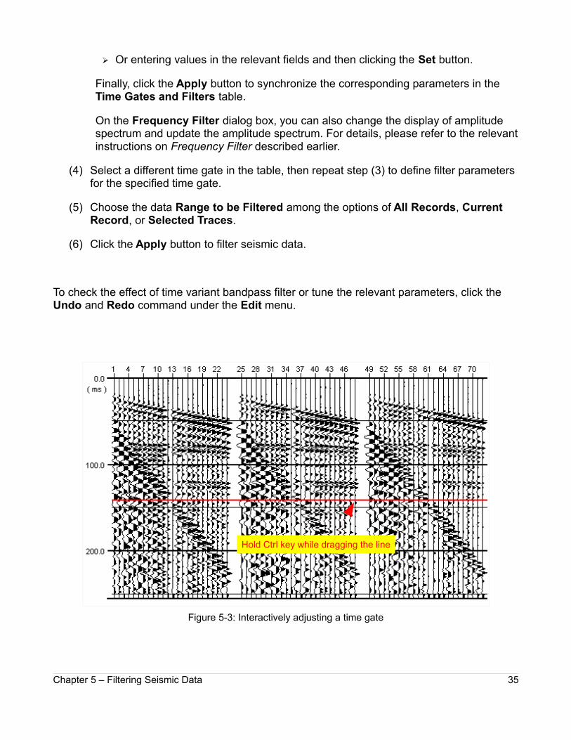
(1) Define the time gate by entering a value in the cell at the End column in the Time Gates and Filters table and then pressing the Enter key, or adjust the time gate by selecting the time gate in the table and then holding down the Ctrl key while dragging the red horizontal line on seismic data in the Display Window as shown in figure 5-3.

To insert a time gate, click the Insert button. To remove a time gate, click the Removebutton.

(2) Select the Butterworth filter or Ormsby filter by clicking the drop-down list box next tothe Filter Type label.

(3) Click the Define Filter button to open the Frequency Filter dialog box as shown in figure 5-4. On the dialog box, set the parameters of Pass and Slope (or Cut for the Ormsby filter) by:

➢ Horizontally dragging the relevant control nodes marked as green dots on the gate curve in the spectrum window.


➢ Or entering values in the relevant fields and then clicking the Set button.

Finally, click the Apply button to synchronize the corresponding parameters in the Time Gates and Filters table.

On the Frequency Filter dialog box, you can also change the display of amplitude spectrum and update the amplitude spectrum. For details, please refer to the relevantinstructions on Frequency Filter described earlier.

(4) Select a different time gate in the table, then repeat step (3) to define filter parameters for the specified time gate.

(5) Choose the data Range to be Filtered among the options of All Records, Current Record, or Selected Traces.

(6) Click the Apply button to filter seismic data.

To check the effect of time variant bandpass filter or tune the relevant parameters, click the Undo and Redo command under the Edit menu.

Figure 5-3: Interactively adjusting a time gate


Hold Ctrl key while dragging the line

Figure 5-4: Defining the time-variant filter parameters on the Frequency Filter dialog box


F-K Filter

F-K filter uses the F-K transform to separate noises and effective signals.

To filter data with F-K filter, open the F-K Filter dialog box by clicking the F-K command underthe Filter menu.

Figure 5-5: The F-K Filter dialog box

On the F-K Filter dialog box as shown in figure 5-5:

(1) Update the F-K spectrum. By default, the spectrum of current record is shown.

To plot the spectrum of a different record, select the record by clicking the left mouse button on seismic data in the Display Window, and then click the Refresh button.

To adjust the spectrum display gain, drag the Display Gain slide bar.

(2) If spatial aliasing occurs, set the shift parameter by entering a value in the Shift field or clicking the arrow button next to the field.


(3) Test the apparent velocity of an event by dragging the left mouse button along the group of waves on seismic data in the Display Window as shown in figure 5-6. Then, move the mouse cursor over the F-K spectrum to check the corresponding apparent velocity shown in the Va field.

(4) Select the Remove range among the Above, Below, Outside, and Inside option, andthen define the range on the F-K spectrum by:

➢ Clicking the left mouse button to insert a control point.

➢ Dragging a control point to adjust the point.

➢ Clicking the right mouse button over a control point to delete the point.

To cancel the defined range, click the Clear button.

(5) Choose the Range to be Filtered between the Current Record and the All Records option.


To check the effect of F-K filter or tune the relevant parameters, click the Undo and Redo command under the Edit menu.

Figure 5-6: Testing the apparent velocity of an event on seismic data


Tau-p Filter

Tau-p filter uses the Tau-p mapping to separate noises and effective signals.

To filter data with Tau-p filter, open the Tau-p Filter dialog box by clicking the Tau-p commandunder the Filter menu.

Figure 5-7: The Tau-p Filter dialog box

On the Tau-p Filter dialog box as shown in figure 5-7:

(1) Select the mapping Mode between the Slowness and Curvature option, and then setcorresponding parameters in the relevant fields, finally click the Refresh button.

If the Curvature option is chosen, the parameters include:

➢ The Type of curvature between the Parabolic and Hyperbolic option.

➢ The maximum frequency in the High End Frequency field.


➢ The number of curvature, minimum curvature, and maximum curvature in the Number, Min, and Max fields.

If the Slowness option is selected, the parameters include:

➢ Number of slowness in the Number field.

➢ Minimum slowness in the Min field.

➢ Maximum slowness in the Max field.

When you input the minimum and maximum slowness in the Min and Max fields, the corresponding maximum and minimum velocities are shown next to the relevant fields.

(2) Update the Tau-p mapping. By default, the mapping of current record is shown.

To plot the mapping of a different record, select the record by clicking the left mouse button on seismic data in the Display Window, and then click the Refresh button.

To adjust the mapping display gain, drag the Display Gain slide bar.

To plot the mapping in color density, turn off the Wiggle option.

(3) Test the apparent velocity of an event by dragging the left mouse button along the group of waves on seismic data in the Display Window as shown in figure 5-6. Then, move the mouse cursor over the Tau -p mapping to check the corresponding apparentvelocity or curvature shown in the Va or Curvature field.

(4) Select the Remove range among the Above, Below, Outside, and Inside option, andthen define the range on the Tau-p mapping by:

➢ Clicking the left mouse button to insert a control point.

➢ Dragging a control point to adjust the point.

➢ Clicking the right mouse button over a control point to delete the point.

To cancel the defined range, click the Clear button.



To check the effect of Tau-p filter or tune the relevant parameters, click the Undo and Redo command under the Edit menu.


Random Noise Attenuation

To apply random noise attenuation on seismic data, open the Random Noise Attenuation dialog box by clicking the Random Noise command under the Filter menu. On the dialog boxas shown in figure 5-8:

(1) Define the Length of Prediction Filter by entering a value in the relevant field or clicking the arrow button next to the field.

(2) Specify the filter Window Size in the Horizontal and Vertical fields.



To check the effect of random noise attenuation or tune the parameters, click the Undo and Redo command under the Edit menu.

Figure 5-8: The Random Noise Attenuation dialog box


Frequency Scan

To run frequency scan, open the Frequency Scan dialog box by clicking the Frequency Scan command under the Filter menu. On the dialog box as shown in figure 5-9:

(1) Modify the number of filters by clicking the Insert or Remove button.

(2) Select the Butterworth filter or Ormsby filter by clicking the drop-down list box below the Filter label.

(3) Enter the parameters of Pass and Slope (or Cut for the Ormsby filter) in the relevant cells at Low Slope(or Cut), Low Pass, High Pass, and High Slope(or Cut) row, and then click the Refresh button to update the plotting in the scan panel.

To change the display of plotting in the scan panel, click the Display button.

(4) Analyze frequencies of another record by clicking the left mouse button on seismic data in the Display Window to select the record and then clicking the Refresh button.

Figure 5-9: The Frequency Scan dialog box


Chapter 6 – Improving S/N Ratio with Deconvolution

This chapter talks about how to improve the S/N (Signal/Noise) ratio with:

➢ Spiking Deconvolution

➢ Predictive Deconvolution

Chapter 6 – Improving S/N Ratio with Deconvolution 43

Spiking Deconvolution

To apply spiking deconvolution on seismic data, open the Spiking Deconvolution dialog box by clicking the Spiking command under the Decon menu.

Figure 6-1: The Spiking Deconvolution dialog box

On the Spiking Deconvolution dialog box as shown in figure 6-1:

(1) Update the Wavelet Definition graph.

By default, the autocorrelation curve of the 1st trace is displayed in the graph.

To update the graph, choose the Autocorrelation or the Current Trace option, then select traces by clicking the left mouse button on a trace or dragging the left mouse button along traces in the Display Window, finally click the Refresh button.

If the Autocorrelation is chosen and there are more than one trace selected, the graph shows the averaged autocorrelation curve.

To cancel the trace selection, move the mouse cursor over a trace on the selected traces in the Display Window and then click the right mouse button or drag the right mouse button along traces, finally click the Refresh button.


(2) Define the wavelet by horizontally dragging the vertical green line on the Wavelet Definition graph.

(3) Select the data Range to be processed between the All Records and the Current Record option.


To check the effect of spiking deconvolution or tune the wavelet definition, click the Undo and Redo command under the Edit menu.


Predictive Deconvolution

To run predictive deconvolution on seismic data, open the Predictive Deconvolution dialog box by clicking the Predictive command under the Decon menu.

Figure 6-2: The Predictive Deconvolution dialog box

On the Predictive Deconvolution dialog box as shown in figure 6-2:

(1) Update the Parameters Definition graph.

By default, the autocorrelation curve of the 1st trace is displayed in the graph.

To update the graph, select traces by clicking the left mouse button on a trace or dragging the left mouse button along traces in the Display Window, and then click the Refresh button. Afterwards, the graph shows the averaged autocorrelation curve.

To cancel the trace selection, move the mouse cursor over a trace on the selected traces in the Display Window and then click the right mouse button or drag the right mouse button along traces, finally click the Refresh button.


(2) Define the filter length by horizontally dragging the red vertical line and then specify the prediction lag by horizontally dragging the blue vertical line on the Parameters Definition graph. The values in the Filter Length field and the Prediction Lag field are correspondingly updated.

(3) Select the data Range to be processed between the All Records and the Current Record option.


To check the effect of predictive deconvolution or tune the relevant parameters, click the Undo and Redo command under the Edit menu.


Chapter 7 – Analyzing Velocities

Before starting velocity analysis:

(1) Sort gathers in common Midpoint (CMP) or common shot point (CSP) order.

For instructions, please refer to Sorting Gathers in Chapter 3.

(2) Load the velocity file previously generated by clicking the Open Velocity command under the File menu.

Skip this step if there is no velocity file available.

Then, analyze velocities with:

➢ Semblance spectra

➢ Velocity scan

At the end, evaluate velocities with NMO and inverse NMO correction.

Chapter 7 – Analyzing Velocities 48

Semblance Spectra

To analyze velocities with semblance spectra:

1 Click the Semblance Spectra command under the VelAnalysis menu. If no velocity file is opened, a dialog box as show in figure 7-1 will appear. Afterwards, click the OK button to launch the Select Velocity File Name dialog box.

Figure 7-1:Reminding to inputting velocity file

2 On the Select Velocity File Name dialog box as shown in figure 7-2, enter a name in the File name field or select an existing velocity file and then click the Save button. Afterwards,the Semblance Spectra dialog box appears.

Figure 7-2: The Select Velocity File Name dialog box


If you select an existing file but the velocities are generated from a different gather order, you will see a dialog box as shown in figure 7-3. You can click the No button to cancel the conversion or click the Yes button to convert velocities and open the Semblance Spectra dialog box.

Figure 7-3: Velocity conversion dialog box

3 On the Semblance Spectra dialog box as shown in figure 7-4:

(1) Define the Velocity Range by entering the minimum velocity, velocity increment, and number of velocities in the Minimum, Increment, and Number fields. Afterwards, the maximum velocity is updated in the Maximum field.

(2) Specify the Sample Interval by entering a value in the Ratio field or clicking the arrowbutton next to the field. Afterwards, the current sample rate is updated in the Current field. For reference, the original sample rate is shown in the Original field.

(3) If the fold of CMP gathers is less than 6, turn on the Super Gather option and enter the number of super gathers in the field next to the option.

If the current gathers are in the CSP order, the Super Gather option is invalid.

(4) Determine how to Stretch the NMO gathers by turning on or off the Auto Mute and Auto Scale options.

If the Auto Mute option is turned on, enter the mute limit and taper in the Limit and Taper fields.

(5) Choose the View options by turning on or off the Local Stack and Velocity Scan Gathers options.

If the Local Stack option is turned on, enter the number of traces to be repeated in the Duplicated Traces field.

(6) Click the Apply or OK button.


Figure 7-4: The Semblance Spectra dialog box

Afterwards, the Display Window is updated as shown in figure 7-5. From left to right are the stacking and interval velocity functions, the semblance spectra, the original CMP or CSP gathers, the NMO gathers plus a local stack if the Local Stack option is turned on, the velocity scan gathers if the Velocity Scan Gather option is turned on, and composite stack overlaid with velocities.

Figure 7-5: The Display Window in velocity analysis with semblance spectra


4 Pick velocities on the semblance spectra in the Display Window as shown in figure 7-5.

➢ To pick a velocity, double click the left mouse button.

➢ To adjust a pick, drag the pick with the left mouse button.

➢ To delete a pick, double click the left mouse button over the pick.

➢ To delete all picks at a location, click the Delete Velocity Function commands under the VelAnalysis menu.

If the Velocity Scan Gathers option is turned on, you can pick velocities on the velocity scan gathers with the same operations.

When velocities are picked, the stacking and interval velocity functions, NMO gathers, and the velocity image overlaid on the composite stack are updated simultaneously. To update the composite stack, click the Build Composite Stack command under the VelAnalysis menu.

5 Select another location and repeat step 4.

To select a location, open the Location Selection for Velocity Analysis dialog box by clicking the Location Selection command under the VelAnalysis menu.

Figure 7-6: The Location Selection for Velocity Analysis dialog box


On the Location Selection for Velocity Analysis dialog box as shown in figure 7-6:

➢ Click the left mouse button on the Location Selection graph to select a location.

➢ Or click the yellow arrow buttons to select a location with a defined increment. To define the increment, enter a value in the Inc field.

➢ Or choose the Select Gather option and then select a location directly on seismic data.

After selecting a location on seismic data, choose the Semblance option to switch the Display Window back to the velocity analysis window.

In addition to using the Location Selection for Velocity Analysis dialog box, you can alsoselect a location directly on the composite stack in the Display Window by clicking the left mouse button on the composite stack.

After a new location is chosen, the velocity function at the nearest location is shown on the semblance spectra for reference. To speed up the picking operations, you can use the Copy Velocity Function and Paste Velocity Function commands under the VelAnalysis menu to copy a velocity function to the current location and then adjust the picks.

6 Save velocities in a text file by clicking the Save Velocity or Save Velocity As command under the File menu.


Velocity Scan

The analyzing steps and operations in the velocity scan are similar to those in the semblance spectra. So the following only talks about the difference.

To analyze velocities with velocity scan:

1 Launch the Velocity Scan dialog box by clicking the Velocity Scan command under the VelAnalysis menu.

2 On the Velocity Scan dialog box as shown in figure 7-7:

(1) Choose the velocity scan method between the Constant and the Percentage option.

(2) If the Constant option is selected, define the Velocity Range by entering minimum velocity, velocity increment, and number of velocities in the Minimum, Increment, andNumber fields.

(3) If the Percentage option is selected, define a velocity function in the Velocity Table by clicking the Add and Remove buttons and then entering values in the relevant cellsat the T and V columns. Afterwards, specify the Percentage Range by entering the minimum percentage, percentage increment, and number of percentages in the Minimum, Increment, and Number fields.


Here, to display the constant velocity stacks on the Stacks of Velocity Scan dialog box as shown in figure 7-8, click the Display Stacks button.

Figure 7-7: The Velocity Scan dialog box


Figure 7-8: Constant velocity stacks

Afterwards, the Display Window is updated as shown in figure 7-9. From left to right are the stacking and interval velocity functions, stacking energy spectra, a constant velocity stack, and the composite stack overlaid with velocities.

Figure 7-9: The Display Window in velocity analysis with velocity scan


3 Pick velocities on the stacking energy spectra in the Display Window as shown in figure 7-9.

➢ To pick a velocity, double click the left mouse button.

➢ To adjust a pick, drag the pick with the left mouse button.

➢ To delete a pick, double click the left mouse button over the pick.

➢ To delete all picks at a location, click the Delete Velocity Function commands under the VelAnalysis menu.

When you pick velocities, the stacking and interval velocity functions, the constant velocity stack, and the velocity image overlaid on the composite stack are updated simultaneously. To manually update the composite stack, click the Build Composite Stack command un-der the VelAnalysis menu.

4 Select another location and repeat step 3.

There are three ways to select a location in the velocity scan:

➢ Use the Location Selection for Velocity Analysis dialog box. For details, please refer to the instructions described in Semblance Spectra.

➢ Click the left mouse button on the constant velocity stack in the Display Window.

➢ Click the left mouse button on the composite stack in the Display Window.

5 Save velocities in a text file by clicking the Save Velocity or Save Velocity As command under the File menu.

To reduce the uncertainty of velocities, combining the semblance spectra and the velocity scan in the velocity analysis is always recommended. You can switch the method by clicking the Semblance or the Velocity Scan radio button on the Location Selection for Velocity Analysis dialog box as shown in figure 7-6.


Velocity Evaluation

To evaluate the velocities generated from velocity analysis:

(1) Create NMO gathers by clicking the NMO Correction command under the NMO menu.

With accurate velocities, the reflection events on NMO gathers should be flattened as shown in figure 7-10. If the reflection events are not flattened enough, the velocities may be inaccurate. Go to step (2) to re-pick velocities.

(2) Cancel the NMO correction by clicking the Inverse NMO Correction command under the NMO menu.

(3) Re-analyze velocities on CMP or CSP gathers with semblance spectra and velocity scan

(4) Repeat step(1)~(3) until the reflection events are flatted on NMO gathers.

Figure 7-10: NMO gathers with accurate velocities

The NMO gathers are also used to build stacks.


Chapter 8 – Applying Static Correction

There are two types of static correction:

➢ Field static correction

➢ Residual static correction

Chapter 8 – Applying Static Correction 58

Field Static Correction

There are two types of field statics: elevation statics and tomo statics.

Elevation Statics

To apply elevation static correction including shot depth correction to seismic data, open the Field Static Correction dialog box by clicking the Field Statics command under the Statics menu.

Figure 8-1: The Field Static Correction dialog box with Elevation option

On the Field Static Correction dialog box as shown in figure 8-1:

(1) Choose the option of elevation statics by clicking the Elevation radio button under the Type label.

(2) Input the final datum in the Datum field.

(3) Input elevation data from:

➢ A text file with the format as shown in figure 8-2 by clicking the File button.

➢ Or seismic trace headers by clicking the Trace Header button.


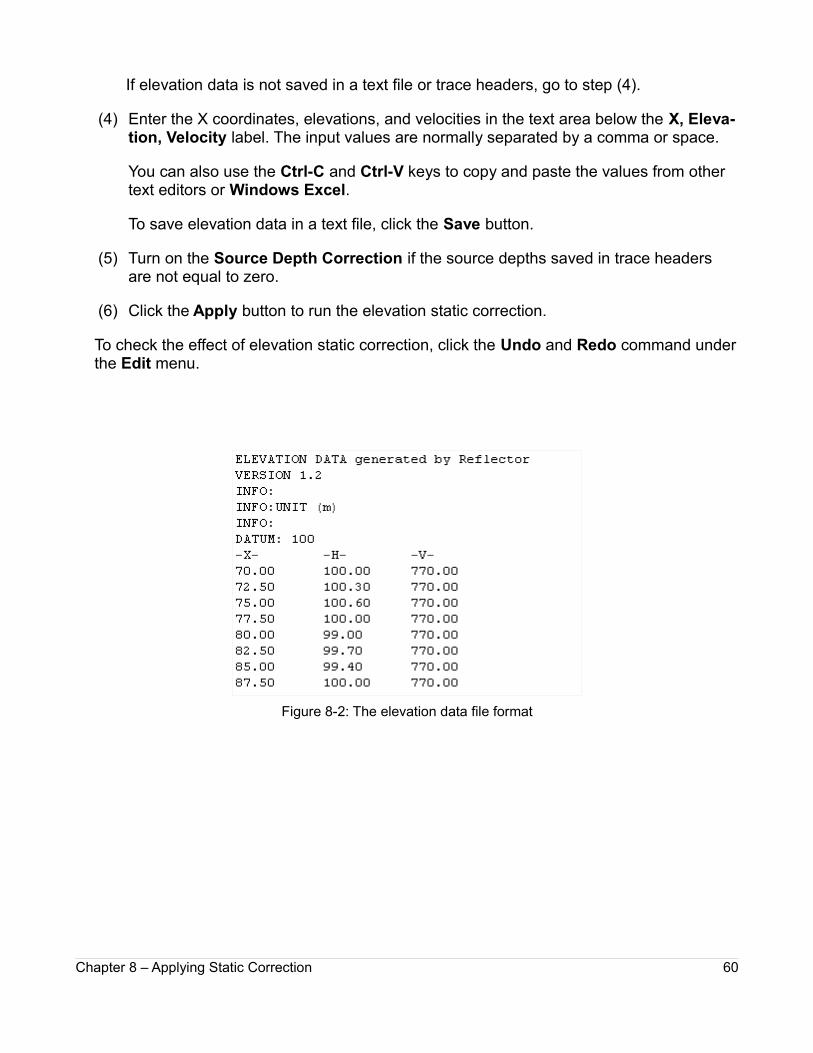
If elevation data is not saved in a text file or trace headers, go to step (4).

(4) Enter the X coordinates, elevations, and velocities in the text area below the X, Eleva-tion, Velocity label. The input values are normally separated by a comma or space.

You can also use the Ctrl-C and Ctrl-V keys to copy and paste the values from other text editors or Windows Excel.

To save elevation data in a text file, click the Save button.

(5) Turn on the Source Depth Correction if the source depths saved in trace headers are not equal to zero.

(6) Click the Apply button to run the elevation static correction.

To check the effect of elevation static correction, click the Undo and Redo command underthe Edit menu.

Figure 8-2: The elevation data file format


Tomo Statics

To apply tomo static correction to seismic data, open the Field Static Correction dialog box by clicking the Field Statics command under the Statics menu. On the dialog box as shown in figure 8-3:

(1) Choose the option of tomo statics by clicking the Tomography radio button under the Type label.

(2) Input the final datum in the Datum field.

(3) Load velocity model from a text file by clicking the Load Velocity Model button. The velocity file is normally generated from Geogiga DW Tomo.

(4) Input the correctional velocity for replacement, datum used in tomography, and depth applied below final datum in the Replacement Velocity, Reference Elevation, DepthApplied fields.

(5) Click the Apply button to run the tomo static correction.

To check the effect of tomo static correction, click the Undo and Redo command under theEdit menu.

Figure 8-3: The Field Static Correction dialog box with Tomography option


Residual Static Correction

The residual static correction should be done on CMP gathers after velocity analysis.

To apply the residual static correction to seismic data, open the Residual Static Correction dialog box by clicking the Residual Statics command under the Statics menu. On the dialog box as shown in figure 8-4:

(1) Enter the maximum shift in samples in the Maximum Shift field.

(2) Enter the number of iterations in the Number of Iterations field.

(3) Select the Stack View.

A CMP stack is automatically created when the Residual Static Correction dialog box appears. You can define a time window on the stack in step(4).

(4) Choose the type of Time Window between the Flat and the Floating option, and thendefine a time window on the CMP stack.

To define the size of time window, enter a value in samples in the Size field.

If the Flat option is chosen, specify the center of the time window by entering a value in milliseconds in the Center field or dragging the green horizontal line drawn on the stack.

If the Floating option is selected, define the time window by clicking the left mouse button on the stack to insert control points as shown in figure 8-5.

➢ To delete a control point, click the right mouse button over the control point.

➢ To adjust a control point, drag the control point with the left mouse button.

(5) Choose the Automatically Refresh option to view the result after an iteration.

To draw a mask on the time window as shown in figure 8-5, select the Mask Time Window option.

(6) Click the Apply button to run the residual static correction.

To check the effect of residual static correction, click the Undo and Redo command under theEdit menu.

Note: If the View option is switched from the Stack to the Gather or vice versa after residual static correction, the Undo and Redo command will be disabled.


Figure 8-4: The Residual Static Correction dialog box

Figure 8-5: Defining a time window on CMP stack


Chapter 9 – Creating Stacks

This chapter talks about how to :

➢ Create a time stack

➢ Run the post-stack time migration

➢ Covert a time stack to a depth stack

➢ Generate instantaneous attributes

➢ Overlay velocities on a stack

Chapter 9 – Creating Stacks 64

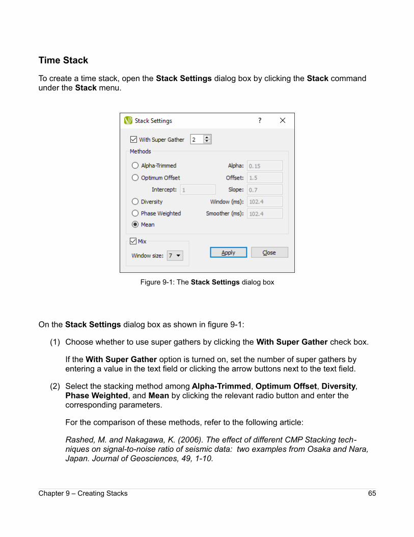
Time Stack

To create a time stack, open the Stack Settings dialog box by clicking the Stack command under the Stack menu.

Figure 9-1: The Stack Settings dialog box

On the Stack Settings dialog box as shown in figure 9-1:

(1) Choose whether to use super gathers by clicking the With Super Gather check box.

If the With Super Gather option is turned on, set the number of super gathers by entering a value in the text field or clicking the arrow buttons next to the text field.

(2) Select the stacking method among Alpha-Trimmed, Optimum Offset, Diversity, Phase Weighted, and Mean by clicking the relevant radio button and enter the corresponding parameters.

For the comparison of these methods, refer to the following article:

Rashed, M. and Nakagawa, K. (2006). The effect of different CMP Stacking tech-niques on signal-to-noise ratio of seismic data: two examples from Osaka and Nara, Japan. Journal of Geosciences, 49, 1-10.


(3) Determine whether to use the mix option by clicking the Mix check box.

If the Mix option is selected, select the Window Size among the 3, 5, and 7 options by clicking the relevant radio button.


Please note: If the gathers are sorted in the common shot order, a CSP stack will be created; otherwise, the stack will be a CMP stack.

To save the time stack, click the Save Time Stack command under the Stack menu.


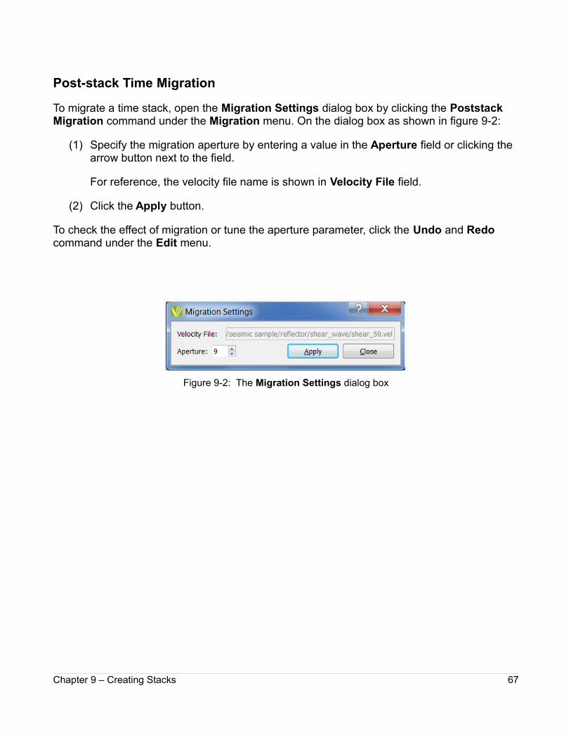
Post-stack Time Migration

To migrate a time stack, open the Migration Settings dialog box by clicking the Poststack Migration command under the Migration menu. On the dialog box as shown in figure 9-2:

(1) Specify the migration aperture by entering a value in the Aperture field or clicking the arrow button next to the field.

For reference, the velocity file name is shown in Velocity File field.


To check the effect of migration or tune the aperture parameter, click the Undo and Redo command under the Edit menu.

Figure 9-2: The Migration Settings dialog box


Depth Stack

To convert a time stack to a depth stack, open the Time-Depth Conversion dialog box by clicking the Time to Depth command under the Stack menu. On the dialog box as shown in figure 9-3:

(1) Enter the Depth Interval and the Number of Depth Samples in the relevant fields.

The maximum depth is simultaneously updated in the Maximum Depth field.

(2) Click the Apply button to create a depth stack.

To save the depth stack, click the Save Depth Stack command under the Stack menu.

Figure 9-3: The Time-Depth Conversion dialog box


Instantaneous Attributes

To create instantaneous attributes after the time stack is built, open the Create Attributes dialog box by clicking the Create Attributes command under the Stack menu. On the dialog box as shown in figure 9-4:

(1) Select the instantaneous attributes to be created by selecting the Amplitude, Phase, Frequency, or Q options.

(2) Click the Create button. Afterwards, the selected attributes are created and plotted in the Display Window as shown in figure 9-5.

To turn on or off some views in the Display Window, choose the Visible options next to the Amplitude, Phase, Frequency, Q, or Seismic options. To change the View Layout, select the Horizontal or the Vertical option.

Figure 9-4: The Create Attributes dialog box

Figure 9-5: The instantaneous attributes in the Display Window


Amplitude Phase Frequency Time Stack

Velocity Overlay

To overlay velocities on a stack as shown in figure 9-6, click the Display command under the Section menu.

Figure 9-6: Overlaying velocities on a stack

To set the display of velocity overlay, open the Section Settings dialog box by clicking the Settings command under the Section menu. On the dialog box as shown in figure 9-7:

(1) Choose the type of stack between the Time and Depth option.

(2) Determine whether to overlay velocities by clicking the Display Velocity checkbox.

If the Display Velocity option is selected, choose the type of velocities between the Stacking and Interval option.

(3) Smooth velocities by choosing the Smooth option and then entering the smoothing Radius in the X and Y fields.



Figure 9-7: The Section Settings dialog box

In addition, the type of data including gathers, time stack, and depth stack can be switched from the list box on the Toolbar as shown in figure 9-8.

Figure 9-8: Switching the view of stacks and gathers


Chapter 10 – Creating a Processing Log

A processing log stores the processing commands and parameters applied to seismic data.

To create a processing log after loading seismic data, open the dockable Log window by clicking the Logging command under the File menu. In the Log window as shown in figure 10-1, you can:

➢ Open and save a processing log file.

➢ Toggle the option to automatically append commands when processing data.

➢ Manually add and delete a processing command.

➢ Import parameters of a selected command to the processing log.

➢ Export parameters of a selected command to the processing dialog box.

Figure 10-1: The Log window

Chapter 10 – Creating a Processing Log 72

Open a processing log file

Save a processing log file

Toggle to automatically append commands

Manually add and delete a processing command

Import parameters of a selected command to the

processing log

Export parameters of a selected command to the

processing dialog box

Chapter 11 – Outputting Results

The results can be:

➢ Printed with a defined size.

➢ Printed as images shown on screen.

➢ Saved as images.

To learn how to print results or save results as images, view Chapter 6 in Getting Started withGeogiga Seismic Pro.

Chapter 11 – Outputting Results 73

Reflector 8.1 User Guide - California Institute of...

Documents

Transcript of Reflector 8.1 User Guide - California Institute of...