Reﬂex motion: masses and orbits - ethz.ch · PDF fileKepler’s law can be generalized...

Chapter 2

Reflex motion: masses and orbits

The mass is a most important parameter for the characterization of an astronomical object.This is also the case for planets. For the planets in the solar system one finds withdecreasing mass: giant planets Jupiter and Saturn, the “ice” giants Neptune and Uranus,the terrestrial planets Earth and Venus with substantial atmosphere, then Mars with onlya thin atmosphere and finally the bare, rocky planet Mercury without atmosphere. Thisanti-correlation between planet mass and extent of the “gaseous” envelope may be alsocommon for extra-solar planets.

The orbit is another key property for a planet. The orbital distance to the star de-fines largely its surface temperature. The orbital eccentricity, inclination, and the mutualorbit geometries in multi-planet systems provide essential information about the dynamicproperties and evolution of a system.

All this information is available without “seeing” the planet, but by measuring thereflex motion of the bright parent stars induced by the planets. The determination ofmasses and orbits based on the reflex motion of unseen companions was introduced morethan 100 years ago for binary stars. But because planets are much less massive thanstars, the required measurement accuracy for extra-solar planetary systems is extremelydemanding and could only be realized with modern technologies. Once, detections ofthe reflex motion were possible, the investigation of extra-solar planetary systems becameimmediately a major new field in modern astronomy, and a substantial fraction of allobservational information on extra-solar planets available today is based on this technique.Mass and orbit determinations via the stellar reflex motion will remain a backbone forextra-solar planet research in the near future. Therefore we discuss these methods in muchdetail.

2.1 Kepler’s laws and the stellar reflex motion

2.1.1 Kepler’s laws

Kepler formulated three generals laws for the orbits of the solar system planets basedmainly on the astrometric data from Tycho Brahe:

1. The planets move on elliptical orbits with the sun located in one of the focal points,

2. the line connecting the sun and a planet sweeps the same area in equal time intervals(Flachensatz),

1

2 CHAPTER 2. REFLEX MOTION: MASSES AND ORBITS

3. The squares of the orbital periods of the planets are proportional to the cubes oftheir semi-major axis.

Kepler’s laws follow also from the 2-body mechanics based on Newton’s theory of gravi-tation for the limiting case M⊙ ≫ mP . They are therefore valid for all 2-body problemswhere one body dominates in mass, for example for moons around planets. We summarizehere important implications of Kepler’s laws. The full derivations of the formula givenin this section can be found e.g. in standard textbooks on mechanics or comprehensivephysics textbooks.

Figure 2.1: Geometry of an elliptic orbit.

First Kepler law (elliptical orbits):

– The eccentricity ǫ characterizes the elliptic orbit 0 ≤ ǫ < 1. The major axis a andminor axis b of the ellipse are related by

b = a√

1− ǫ2 . (2.1)

– The location of the sun in the focal point F is offset from the ellipse center by thedistance a · ǫ on the major axis. The perihel rmin and aphel rmax distances are

rmin = a (1− ǫ) and rmax = a (1 + ǫ) .

– For circular orbits there is ǫ = 0 and a = b = rmin = rmax.

– For ǫ → 1 the orbit approaches a parabola (ǫ = 1) which is not a closed orbit.

Second Kepler law (Flachensatz):

– The second Kepler law is equivalent to the conservation of angular momentum ~L =mP~v × ~r

∆A =1

2|~x× ~v|∆t =

1

2mP|~L|∆t ,

where ∆A is the swept area per time interval ∆t.

2.1. KEPLER’S LAWS AND THE STELLAR REFLEX MOTION 3

– The second Kepler law can also be written as

∆A

πab=

t− T0

P, (2.2)

where T0 is the time of perihel passage and P the orbital period. From this rela-tionship one can derive numerically (not analytically) the “central” orbital angle Efrom the mean orbital anomaly M = E(t)− ǫ sinE and then the orbital phase angleas function of time φ(t) from

tanφ(t)

2=

√

1 + ǫ

1− ǫtan

E(t)

2where E(t)− ǫ sinE(t) =

2π

P(t− T0) .

The radial distance is defined by the orbital phase angle and the eccentricity

r(φ) = a1− ǫ2

1 + ǫ cosφ, (2.3)

– The orbital velocity has a maximum at perihel and a minimum at aphel

vmax =2πa

P

√

1 + ǫ

1− ǫand vmin =

2πa

P

√

1− ǫ

1 + ǫ,

which becomes of course a constant orbital velocity v = 2πa/P for a circle (ǫ = 0).

Third Kepler law:

– The third Kepler law states that a3/P 2 = const for the solar system planets. Theconstant is directly related to the mass of the sun and therefore the third Kepler lawis a most important tool for the determination of the the mass M of an astronomicalobject by measuring the separation and the orbital period of a small companionm ≪ M :

a3

P 2=

G

4π2M , (2.4)

where G is the gravitational constant.

– For circular orbits the velocity vcirc is related to a and P by vcirc = 2πa/P so thatthe above relation can be written as

v3circ · P = 2πGM .

indicating that the mass of the central object can also be determined by measuringthe orbital velocity vcirc and the period P .

– The third Kepler gives also the orbital velocity of small objects around a centralmass M as function of distance. For circular orbits P = 2πa/vcirc there is

vcirc =

√

GM

a∝

√

1

a. (2.5)

– The third Kepler law follows also from the force equilibrium −FG = FZ for a circularorbit, where the gravitational force is FG = −GMm/r2 and the centrifugal forceFZ = mω2r (where r = a and the angular velocity ω = 2π/P ).


2.1.2 Generalization for a two body problem

Kepler’s laws follow from Newton’s two body problem with M1 and M2, for the specialcase where M1 = M ≫ m = M2 → 0. Kepler’s law can be generalized for the two bodyproblem with M2 > 0:

– The exact formula for Kepler’s third law for a 2-body system is

(a1 + a2)3

P 2=

G

4π(M1 +M2) . (2.6)

– The individual orbits of the two masses M1 and M2 are ellipses with eccentricityǫ and semi-major axis a1 and a2 respectively, with the center of mass at the focalpoints. The total semi-major axis a of the orbit of M2 with respect to M1 is

a = a1 + a2 .

– The semi-major axis of the two ellipses behave like

M1a1 = M2a2 , (2.7)

according to the lever rule (Hebelgesetz). The radial distances and orbital velocitiesbehave accordingly

M1r1(φ) = M2r2(φ) and M1v1(φ) = M2v2(φ) .

2.1.3 Orbital elements

Seven quantities are necessary for the definition of the elliptic orbit of an object in a twobody system. If the orbit of one object M1 or M2 is given relative to the center of massthen the ellipse has the semi-major axis a1 or a2 respectively. If the orbit of one object isgiven relative to the position of the other object then the semi-major axis is a = a1 + a2.One object needs to be identified for the definition of the position angle for the orientationof the orbit, because the other object has an orbit which is offset by 180 in orbital phasewith respect to the first object.

Four parameter describe the elliptical orbit:

– P : Orbital period,

– ǫ: eccentricity of the ellipse,

– T0: time of periastron (or perihel) passage,

– a1, a2, or a: semi-major axis of the ellipse of component 1, component 2, or of onecomponent relative to the other component.

Three quantities describe the orientation of the elliptical orbit on the sky:

– Ω: position angle of the line of nodes for the orbital plane and a reference plane withrespect to a reference point. In the case of a solar system object this is the eclipticplane and the ”March” equinox. For a stellar system this is the sky plane and theposition angle with respect to N (measured from N over E).

– i: inclination of the orbital plane with respect to the reference plane (ecliptic or skyplane)

– ω: Angle between the line of node and the periastron (or perihel) passage. For astellar system this can be defined e.g. by the angle from the line of node passagewith positive radial velocity (red shift).

2.1. KEPLER’S LAWS AND THE STELLAR REFLEX MOTION 5

Figure 2.2: Illustration for the definition of the orientation of the elliptical orbit.

2.1.4 Orbital parameters for the solar system planets.

Table 2.1 gives orbital parameters for the solar system planets.

Table 2.1: Masses and orbital parameters for solar system planets. P is the orbital period,a the semi-major axis, v the mean orbital velocity, ǫ the eccentricity, and i the inclinationwith respect to the ecliptic plane.

planet M [MJ] P [yr] a [AU] v [km/s] ǫ i

Mercury 0.00017 0.241 0.387 47.9 0.206 700′′

Venus 0.0026 0.670 0.723 35.0 0.007 324′′

Earth 0.0031 1.00 1.00 29.8 0.017 000′′

Mars 0.00034 1.88 1.52 24.1 0.093 151′′

Jupiter 1.0 11.9 5.20 13.0 0.048 119′′

Saturn 0.299 29.5 9.55 9.64 0.056 230′′

Uranus 0.046 84.0 19.2 6.80 0.046 046′′

Neptune 0.054 165. 30.1 5.43 0.009 147′′

MJ = 1.90 · 1027 kg, 1 year = 365.25 days, 1 AU = 1.50 · 108 km

2.1.5 Expected reflex motion due to planets

The reflex motion of a star due to orbiting planets follow from Newton’s mechanics. Thestar will circle around the center of mass of the planetary system and mirror the motionof the planets. This motion can be measured with three different techniques:

– Radial velocity: periodic radial velocity variation of the star with respect to theline of sight, which can be measured with high precision spectroscopy,

– Astrometric motion: periodic motion of the star around the center of mass in thesky plane which can be measured with high precision astrometric techniques,

– Timing variation: arrival time variations of a well defined periodic signal due tolight path variations or changes in the system configurations.


The expected motion of the sun as seen from a distance of 10 pc is shown in Slide 2.1 andTable 2.2 gives the values induced by Jupiter and Earth. The solar motion is dominatedby the reflex motion due to Jupiter which has a period of 12 years. The typical amplitude(radius) of the circular motion is about 0.005 AU = 7.5 · 105 km (0.001′′ at 10 pc is 0.01AU). This orbit is comparable to the radius of the sun.

Table 2.2: Typical values for observables for the reflex motion for Jupiter-like and Earth-like planets (mass and orbit) around a solar mass star.

observable Jupiter Earth meas. limit (2013)

radial velocity amplitude 12.8 m s−1 0.1 m s−1 ≈ 1 m s−1

astrometric amplitude d = 10 pc 500 µas 0.3 µas ≈ 1 masastrometric amplitude d = 100 pc 50 µas 0.03 µas ≈ 1 mas

timing residuals 2.5 s 1.5 ms depends on signal

The time dependence of the measured reflex motion provides orbital parameters like pe-riod, eccentricity etc., while the amplitude of the observed effect is proportional to theplanet mass. If the mass of the star is known then one can estimate the mass of theplanet. The different methods provide not exactly the same information and they favorthe detection of different kinds of systems as summarized in Table 2.3.

Table 2.3: Resulting planet parameters from measurements of the reflex motion.

method mass orbit favored systems

radial velocity Mp sin i P, T0, ǫ, a sin i, ω shorter period planets, around bright,quiet stars with many absorption lines

astrometry Mp P, T0, ǫ, a, i, ω,Ω longer period (> 1 yr) planets aroundnearby stars

timing residual Mp sin i P, T0, ǫ, a sin i, ω measurable only for stars with well de-fined periodic signal

2.2. RADIAL VELOCITY METHOD 7

2.2 Radial velocity method

2.2.1 The radial velocity signal

With the radial velocity method one can only measure the velocity component of the starparallel to the line of sight vr = dz/dt. We consider here the effect of one planet only. Inthis case the temporal dependence of the z-component of the orbit is

z(t) = rS(t) sin(ω + φ(t)) sin i , (2.8)

where, sin i is the inclination of the orbital plane with respect to the line of sight, and ωthe orientation of the periastron phase away from the line of sight.

The resulting radial velocity signal induced by a planet follows by differentiation ofEquation 2.8, the ellipse equation, and Kepler’s 2nd law as given below:

vr(t) =dz(t)

dt=

2π

P

aS sin i√1− ǫ2

(

ǫ cosω + cos(ω + φ(t))

(2.9)

For the observed radial velocity there is in addition a (usually) constant radial velocity ofthe center of mass v0

vr(t) = v0 +K(

ǫ cosω + cos(ω + φ(t))

with K =2π

P

aS sin i√1− ǫ2

. (2.10)

K is called the RV semi-amplitude of the stellar reflex motion which is relevant for thedetermination of the planetary mass. The term in the brackets defines the shape of theperiodic radial velocity curve. The only time-dependent quantity is φ(t) as described inSection 2.2.

The following equation provide the derivation of Equation 2.9 from Equation 2.8 using the ellipseequation and Kepler’s 2nd law (see Section 2.2). Derivation yields:

dz

dt= sin i

dr

dtsin(ω + φ) + r cos(ω + φ))

dφ

dt.

The derivation dr/dt follows from the ellipse equation r = a(1− ǫ2)/(1 + ǫ cosφ)

dr

dt= − a(1− ǫ2)

(1 + cosφ)2(−ǫ sinφ)

dφ

dt=

ǫ sinφ

a(1− ǫ)2r2

dφ

dt.

One can replace r2 dφ/dt according to the 2nd Kepler law

r2dφ

dt=

2π

Pab =

2π

Pa2√

1− ǫ2

and r dφ/dt follows by dividing the Kepler law with r (ellipse equation)

dr

dt=

2π

Pa

ǫ sinφ√1− ǫ2

and rdφ

dt=

2π

Pa1 + ǫ cosφ√

1− ǫ2.

Inserting these two relations in dz/dt and using as a trick the following trigonometric relation

cosω = cos(

(ω + φ)− φ)

= cosφ cos(ω + φ) + sinφ sin(ω + φ)

yields then Equation 2.9 for the radial velocity variation.


Mass for the planet. From the radial-velocity parameters K, P and ǫ follows aS , thesemi-major axis for the orbit of the star around the center of mass

aS sin i =P

2π

√1− ǫK . (2.11)

Using Kepler’s third law a3/P 2 = G(mS + mP )/4π2, a = aS + aP and mSaS = mPaP

yields the so called mass function

(mP sin i)3

(mP +mS)2=

P

2πGK3(1− ǫ2)3/2 . (2.12)

For planetary systems there is mP ≪ mS and one can use for the mass of the planet theapproximation

mP sin i ≈( P

2πG

)1/3Km

2/3S

√

1− ǫ2 . (2.13)

Thus one can derive the mass of the planet mP sin i from the radial velocity data providedthat the mass of the central star mS is known. Usually mS is known within an uncertaintyof a few percent. The inclination factor sin i cannot be determined with RV-data alone.

Impact of the “sin i”-factor. With the radial velocity method alone one can get theplanet mass mP only together with the unknown sin i factor for the orbit inclination. Themeasured value mP sin i is therefore a lower limit value, also called minimum mass for aplanet. Thus one needs to consider that a given system could be seen almost pole-on, withan orbit inclination close to i ≈ 0 or sin i → 0. In such cases the planet mass is stronglyunderestimated.

If one assumes a random orientation of the orbital planes then the distribution oforbital inclinations is n(i) ∝ sin i. The probability to have a system within the inclinationrange [0,ix] is

∫ ix

0

sin i di = 1− cos ix

Thus, only 13.4 % of all systems have i < 30 or sin i < 0.5 and therefore a mass whichis more than twice the measured minimum mass. 71 % of all systems have i ≥ 45 andsin i > 0.71 and 50 % i ≥ 60 with sin i > 0.86 and the real mass of the planets isunderestimated less than about 30 % or 15 % respectively.

Convenient formulae. The formulae derived above can be expressed in convenientunits. The planet mass is:

mP [MJ ] sin i ≈ 3.5 · 10−2K[m s−1] (P [yr])1/3 (mS [M⊙])2/3 .

The semi-major axis a of the orbit of the planet relative to the star follows from the 3rd

Kepler law. With the approximation mP ≪ mS and one can write

a[AU] ≈ (P [yr])2/3(mS [M⊙])1/3

Similarly one can express the radial velocity semi-amplitude for given system parameters:

K =28.4m s−1

√1− ǫ2

mp[MJ ] sin i( 1

mS [M⊙]

)2/3( 1

P [yr]

)1/3

2.3. MEASUREMENT OF RADIAL VELOCITIES 9

2.2.2 Examples for the radial velocity signal induced by planets

Slide 2-2 to 2-4 illustrate a few examples for measured RV-curves for extra-solar planetarysystems:

51 Peg b: Slide 2-2 shows the historical detection measurements for 51 Peg b, the firstextra-solar planets around a normal star, from Mayor and Queloz. The orbital period isabout 4.2 days and the RV-semi-amplitude 59 m/s. The scatter of the data points withrespect to the fit is 13 m/s. The measurements which were taken during many differentorbits have been folded into a phase curve.

HD 4113 system: Slide 2-3 shows the RV-measurements and the phase curve for alonger period (529 days) planet with a very high eccentricity of ǫ = 0.90. In addition thereis a long term trend which points to a brown dwarf or low mass star with an orbit > 20years. A good sampling and long term monitoring are essential to uncover the real natureof such systems. Clearly visible are the yearly observing seasons for this object. Only4 orbital periods (≈ 6 years) after the initial detection of RV variations the very shortperiastron passage could be sampled with observation. The definition of the orbit of theouter companion must be completed by the next generation of astronomers.

HD 40307 system: State of the art measurements of the three super-Earth system HD40307 are shown on Slide 2-4. A measuring precision of ≈ 1 m/s is required to achieve thedetection of planets which induce RV-variation with a semi-amplitude of K = 2− 5 m/s.Multi-planet systems like this one require many data points to reveal the very complicatedRV-pattern. From a few data points one would interpret the data just as noise inducedby the instrument or the central star. A careful analysis is required to extract finally thecorrect solution.

2.3 Measurement of radial velocities

2.3.1 Science requirements.

A very high measuring precision is required for the detection of the planet induced reflexmotion of stars. The Doppler effect gives the relation between radial velocity vr and therelative wavelength shift ∆λ/λ, which is:

vrc

=∆λ

λ(2.14)

If one aims to achieve an accuracy of ∆v = ±3 m/s. then this corresponds to a measuringprecision of

±∆λ

λ=

±∆vrc

=±3 m/s

300′000 km/s= ±1 · 10−8 . (2.15)

The next generation of instruments aims at an accuracy which is another order of mag-nitude higher. What this very demanding science requirement really means is illustratedin Slide 2-5. The slide shows a section of the solar absorption line spectrum and picks asingle line which is then compared to the shift expected by the radial velocity variationinduced by a planet. The effect is much smaller than the line widths. It is obvious that


the technical requirements for building such a measuring instrument are very demandingand require sophisticated techniques.

In the following sections we introduce first the basic principles for astronomical spec-troscopy before addressing the details of the modern RV measuring techniques.

2.3.2 Telescopes

Basic principles of a telescope We first consider the astronomical refractor to explainthe basic layout of telescopes. The astronomical refractor consists of:

– a converging (convex) objective lens or aperture lens,

– an intermediate focus with eventually a field stop,

– a collimating lens,

– a parallel beam section with an intermediate pupil,

– a converging lens (camera lens).

Figure 2.3: Basic principles of a telescope.

The following quantities are used to describe a telescope:

– f1: focal length of objective lens L1,

– f2: focal length of the collimating lens L2 (or the eyepiece),

– f3: focal length of the camera lens L3,

– y1: or D, the diameter of the entrance pupil or aperture,

– y2: diameter of the intermediate pupil,

– α: semi-angle of the field of view in the entrance pupil,

– θ: semi-angle of the field of view in the exit pupil.

Some basic principles are:

– An image of the object is formed in the focal planes. The image plate scale is definedby the effective focal lengths f given by the F -ratio of the image forming lens L1 orL3 and the diameter of the entrance pupil D:

f = Fx ·D . (2.16)


– In a pupil plane the light from a distant object forms parallel rays. The informationis in the angular direction of the rays. In the case of the astronomical refractor thecollimating eyepiece refracts the light into a more or less parallel beam suited forobservation with the eye. The magnifying power m (angular magnification) of thetelescope is:

m =f1f2

=tan θ

tanα=

y1y2

. (2.17)

– The collimated beam section between L2 and L3 is the typical location for diffractiongratings or prisms for spectroscopy.

– The field stop in the first focal plane can be used for field selection (e.g. a spectro-graph aperture) or for a coronagraphic mask.

– Well designed pupil and field stops can be very helpful in reducing the stray lightand the background level of an instrument.

2.3.3 Spectrographs

Equations for grating spectrographs. A diffraction grating consists of a large num-ber of very fine, equally spaced parallel and periodic slits separated by a. The waveletsfrom each slit are strongly enhanced in a few directions θn in which all the wavelets are inphase so that constructive interference occurs. θ1 is the first order with a path differenceof λ etc. For wavelength λ the angular displacement θm is

sin θm =m · λa

, (2.18)

where a is the periodic separation between the grating lines and m an integer number forthe interference order. Because θm depends on λ the light is dispersed and spectra areformed. One should be aware that an overlap of the different orders (m − 1, m, m + 1,etc.) can occur. The same effect is obtained for a reflection grating which has fine periodicrulings.

Figure 2.4: Principle of a spectrograph grating.

The angular dispersion dθ/dλ of the grating follows from differentiation (determine firstdλ/dθ):

dθ

dλ=

m

a cos θ.


The angular width Wθ of a monochromatic interference peak is broad for few grating linesand it becomes narrower as the number of illuminated grating lines N increases like

Wθ =λ

Na cos θ.

This width can also be expressed in a wavelength width ∆λ

∆λ = Wθdλ

dθ=

λ

Na cos θ· a cos θ

m=

λ

N m,

or a resolving power R for a more general characterization of the diffraction limited reso-lution of the grating

R =λ

∆λ= N m. (2.19)

This formula indicates that the resolving power depends only on the number of illuminatedgrating lines N and the dispersion order m.

Gratings, in particular reflective gratings, are often inclined with respect to the incomingbeam by an angle i which is the angle of the grating normal to the incoming beam. Theangle θ is then defined by the interference orderm and the zero order. In this case Equation(2.18) includes the term sin i for the grating inclination:

sin θ =m · λa

− sin i . (2.20)

This is called the grating equation. The resolving power is larger for inclined gratingsbecause more lines are illuminated for a given beam diameter

R =λ

∆λ=

N m

cos i. (2.21)

The grating equation describes also how one can change the central wavelength and thewavelength range for a given deflection angle θ by changing the tilt angle i. The followinglist gives the dependence of spectrum parameters on grating properties:

– the resolving power R depends only on the number of illuminated lines and thediffraction order

– R increases if the number of lines per mm of the grating are enhanced for a givenbeam (=pupil) diameter

– R can be enhanced for a given grating by a larger illuminating beam (larger pupil)or by tilting the grating so that the illuminated lines increase like Ni = Ni=0/ cos i

– R is substantially larger for higher diffraction orders R ∝ m (there is the restrictionthat overlap of grating orders occur)

– the wavelength region for a given deflection angle can be selected by changing theinclination i of the grating.


2.3.4 Different types of spectrograph gratings

Simple gratings. Typical grating have about 100 − 1000 rulings/mm. This yields forthe first order diffraction spectrum and a collimated beam diameter (pupil diameter) of1 cm a grating resolving power of R = 1000 − 10000. The first order spectrum can becontaminated by the second order spectrum with λm=2 = λm=1/2 or higher order spectraλm≥3. For ground based optical spectroscopy this happens for λm=1 > 660 nm, whensecond order light from above the UV-cutoff λm=2 > 330 nm sets in. The second ordercan be suppressed with a short wavelength cutoff filter. For example a BG430 filter cutsall light short-wards of about 430 nm, allowing first order spectroscopy from 430 nm to860 nm without second order contamination.The same grating can also be used in second order with twice the resolution of the firstorder. In this case one has to select for a given wavelength range the correct pass-bandfilter to avoid the contamination by other orders.

Blazed gratings. Simple gratings are not very efficient since the light is distributedto several grating orders. The efficiency of reflecting gratings can be improved by anoptimized inclination of the reflecting surfaces so that they reflect the light preferentiallyin the direction of the aimed interference order. Thus the grating efficiency is optimizedfor one particular wavelength or diffraction angle θb, the so-called blaze angle.

Figure 2.5: Illustration of a blazed grating and an echelle grating.

Echelle gratings. An extreme case of the blazed grating is the echelle grating. It isstrongly inclined with respect to incoming beam and more importantly it is optimized(blazed) for high order diffraction directions, say m = 10− 100. With this type of gratingthe resolving power can be strongly enhanced even if the grating is quite coarse. Forexample a beam of 2 cm diameter illuminating an echelle grating with 20 lines / mm,inclined by i = 60 (1/ cos i = 2) will see effectively 800 grating lines, which producefor m ≈ 50 a spectral resolving power of R = 40′000. Of course for such a grating thefree spectral range, without overlap by neighboring pixels, is only small and of the order∆λ ≈ λ/m. Narrow band filters are required to select one particular order.A more elegant solution is a cross dispersion with a second low order grating or a prismperpendicular to the dispersion of the echelle grating. In this way the individual orders


are displaced with respect to each other and many orders of the echelle grating can beplaced on a rectangular imaging detector.

2.3.5 Technical requirements for a RV-spectrograph

The scientific requirement for measuring radial velocities with a precision of 3 m/s im-poses very demanding technical requirements for a spectrograph. The following type ofmeasurement must be possible:

– a spectral resolving power R = λ/∆λ > 50′000 is required for resolving the individualspectral lines and measure small wavelength shifts,

– a broad spectral coverage is required to cover many thousand lines for higher effi-ciency or for achieving enough signal for a successful detection,

– a high spectrograph throughput and/or a large telescope which allows also a searchfor planets around faint low mass stars or more distant stars,

– an efficient measuring and calibration strategy,

– a telescope with enough available observing time for monitoring program.

For achieving these technical requirements there are various problems and instrumenteffects which must be under control. The following effects introduce shifts which can be 2or 3 orders of magnitudes larger than the required precision of 3 m/s:

– The variation in the index of refraction of air nair with temperature or pressureintroduces strong wavelength shifts. The measured wavelengths is

λmeas = nair(P, T )λvac

where λvac is the wavelength in vacuum. A temperature change of 0.1 K or a pressurechange of 0.1 mbar introduce a wavelength shift of about 10 m/s! These large am-plitude drifts must therefore be corrected with very high accuracy. This is achievedwith the simultaneous measurement of a calibration spectrum.

– Mechanical flexures introduced by thermal expansion or variations in mechanicalforces can cause substantial shifts of the spectrum on the detector. The typicalvelocity sampling on the detector is about 1 km/s per pixel, with pixels dimensionsof about 10 - 20 µm. Thus a measured wavelength shift of 3 m/s corresponds onthe detector to a physical shift of the spectrum of about 50 nm. Any uncalibratedinstrumental flexure at this level is very harmful.

– The spectrograph illumination must be very stable. If the illumination is not fullystable due e.g. to telescope guiding errors, then this may introduce variable illumi-nation gradients which may cause large spurious wavelength shift. An absorptioncell in front of the spectrograph aperture or a spectrograph illumination with a fiberare two approaches to solve this problem.

These are only the most important disturbing effects which must be considered. Otherissues are the definition of accurate wavelengths of the spectral reference (to 9 or 10 digits),the stability of the spectral reference, detector effects like non-perfect charge transferefficiency and other problems.


2.3.6 HARPS - a high precision radial velocity spectrograph

HARPS is currently the best instrument for the measurement of reflex motion of planetarysystems. HARPS is an echelle spectrograph at the ESO 3.6m telescope which was builtas dedicated planet search instrument. It can measure radial velocities to a precision of∆RV = ±1 m/s or even a bit better.

HARPS is optimized for stability and the instrument has no moving components.The light of a star is focussed by the telescope onto an entrance lens of an optical fiberwhich guides the light to the spectrograph located in a laboratory. Using a fiber hasthe advantage that it equalizes inhomogeneous illumination from the telescope due to themany internal light reflections. Thanks to this the illumination of the spectrograph is veryhomogeneous.

The HARPS spectrograph is located in a temperature controlled vacuum vessel (Slide2.6) to minimize drifts due to temperature and air pressure variations and thermal vari-ations in the instrument. Simultaneously with the target a second fiber is illuminatedwith a Th-Ar spectral reference light source which provides a rich and accurate referencespectrum for the calibration of each individual measurement. The spectral range coveredis 378 nm – 681 nm with a spectral resolving power of about R = ∆λ/λ = 90′000. Theresulting data format of the echelle spectrograph is shown on Slide 2-7.

The main components of HARPS are:

– one fiber head for the target at the Cassegrain focus of the ESO 3.6 m telescope,

– a second fiber input which can be fed by a ThAr emission line lamp,

– an echelle grating, 31.6 gr/mm with a blaze angle of 75 with dimensions of 840 ×214× 125 mm (Slide 2-6),

– collimator mirror with a diameter of 730 mm (F = 1560 mm), which is used in triplepass mode,

– cross disperser grism (a combination of transmission grating and prism) with 257lines/mm,

– two 2k × 4k CCD detectors which record the echelle grating orders m = 89− 161 ina square image plane.

The HARPS spectrograph achieves a spectral resolution (≈ 3 pixels) of about ∆λ =0.005 nm or 50 mA. This allows us to measure wavelength shifts of the order 10−6 nmprovided there are a large number, say > 10′000, of narrow lines with a width of ≈ 0.02 nmin the spectrum. The measured wavelength shift corresponds to a physical shift of thespectrum of about 10 nm on the detector or ≈ 1/1000 of a detector pixel.

2.3.7 Stellar limitations to high-precision radial velocity

Measuring the reflex of motion of a star to a precision of ∆v ≈ ±3 m/s requires that thestellar properties are favorable for such a measurement. The ideal target for radial velocitymeasurements are bright, G or K main-sequence star (mass range 0.7− 1.2M⊙) with verylow magnetic activity. Of course one would like to investigate planetary systems not onlyaround such stars but for a broad range of systems with different stellar parameters.


Figure 2.6: Stars in the Hertzsprung-Russell diagram and their usefulness for the radialvelocity search of planets.

Radial velocity search for different stellar types. We consider different types ofstars in the Hertzsprung-Russell diagram in Fig. 2.6 and discuss their suitability for radialvelocity searches of planets.

– G and K main-sequence stars: These are often the ideal targets for the RV-searchof planets. They have a very rich absorption spectrum and they are also sufficientlyfrequent and bright for a statistically representative sample (> 500 objects). Gand K stars younger than 1 Gyr are still rotating quite fast and therefore theiratmosphere is not stable enough for very accurate measurements. We will discussthis further below.

– F main-sequence stars: Late F-stars can be good targets like G stars but forearly F-stars the lines are quite broad and the rotational induced activity is often aproblem. Atmospheres of F-stars show quite often stellar oscillations (see Slide 2.8for an example).

– A stars: A stars are problematic for planet searches with the RV method. Hotstars have less absorption lines and their widths are strongly enhanced by pressurebroadening and rotation. For example the bright A stars Altair and Fomalhautshow line broadening due to a rotation speed of vrot sin i = 240 km/s and 93 km/srespectively. Therefore it is currently only possible to find for A stars the reflexmotion with K ∼> 30 m/s. Only giant planets with short orbital periods < 1 yearcan be found around these stars.

– M type main sequence stars: Old M-stars are often objects with very stable at-mospheres well suited for radial velocity measurements. M stars younger than about1 Gyr are often too active (like young G and K stars) for accurate RV-searches. Animportant problem is that M-dwarfs are faint in particular in the visual wavelengthrange. Larger telescopes and RV-spectrographs optimized for the near-IR wave-lengths are required to investigate better M-stars with high precision.


– G- and K-giants: These are evolved A- and late B-stars located on the giantbranch in the HR-diagram. Because they have a rich spectrum of narrow lines theycan be used to assess planets around stars with a masses ∼> 1.5M⊙ (what is difficultfor main sequence stars).

– Other stars: High-mass stars and luminous red giants are not suited for radialvelocity searches of planets. Hot, high mass stars and white dwarfs have only few,broad lines. Red giants show at least strong, disturbing atmospheric oscillations (atthe 1 km/s level) if not large amplitude pulsations (> 10 km/s). It seems impossibleto measure for such star the potential reflex motion due to a planet.

Magnetic activity of late type stars. As discussed above only late type main se-quence stars of spectral type F, G, K and M and subgiants or giants of spectral type Gand K are suited for sensitive K < 30 m/s radial velocity searches of planets.

For a RV search in the range ∆RV ≈ m/s for low mass planets one needs to addressthe disturbing effects from the stellar atmosphere in more detail. All late type stars havea convective outer envelope and they are born as rapid rotators with rotation periods ofa few days. Convective motion and fast rotation induces a dynamo effect and thereforestrong magnetic activity which is disturbing the RV measurements. With age the rotationslows down due to the loss of rotational angular momentum via a magnetized stellar wind.For this reason, old stars show much less activity and are therefore better targets for verysensitive radial velocity searches. For comparison, our sun with an age of 4.6 Gyr is arather old and inactive star with a long rotation period of about one month. It would besuited for the search of planets.

Disturbing effects which are introduced by magnetic activity:

– stellar rotation and spots,

– magnetic suppression of convective surface motion,

– stellar oscillations.

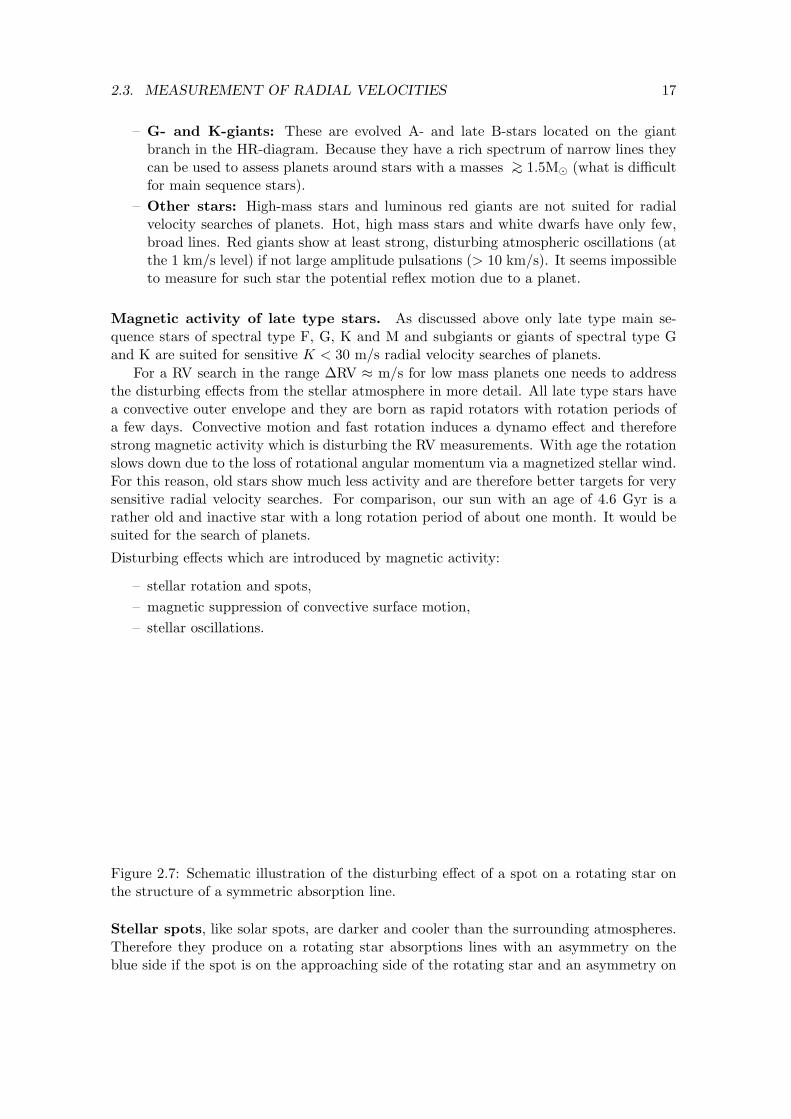
Figure 2.7: Schematic illustration of the disturbing effect of a spot on a rotating star onthe structure of a symmetric absorption line.

Stellar spots, like solar spots, are darker and cooler than the surrounding atmospheres.Therefore they produce on a rotating star absorptions lines with an asymmetry on theblue side if the spot is on the approaching side of the rotating star and an asymmetry on


the red side if the spot is on the receding side of the star. Because the spot is cool, it willproduce a deeper absorption for low excitation lines (e.g. from neutral atoms an molecules)while the spot absorption are less deep for high excitation lines from e.g. ionized species.Overall, the impact is a systematic displacement of line centers which can significantlyaffect the RV-measurement of a planet search program. An example for the resultingRV-signal induced by spots is shown for α Cen B in Slide 2.9.

Convection at the surface of late type stars is suppressed slightly by magnetic activityand the presence of stellar spot. Because the upward motion is less strong, we see less gaswith strong velocity components towards us and the average RV of the star is red-shifted.This effect is stronger during active phases of the magnetic cycle of stars. For the sun themagnetic activity goes up and down on a cycle with a periodicity of 11 years.

For extra-solar planet search programs these activity cycles can be very disturbingbecause a very quiet star may turn suddenly into an active star and introduce muchenhanced intrinsic RV-velocity variations (see Slide 2.9). For the analysis of RV-datait is important to check always the activity status of a star. A good activity indicatorare the Ca ii H and K lines, which have for active phases an enhanced central emissioncomponents.

Figure 2.8: Schematic illustration of the Ca ii emission cores in active late type stars.

Stellar oscillations are induces by the convective gas motion in the envelope. Oscillationsare often quite strong for F-stars, because they are located in or close to the pulsationinstability strip in the HR-diagram. Typical periodicities of the stellar oscillation are ofthe order several minutes and the induced RV-shift can be of the order 10 m/s (see Procyonon Slide 2.8) but also much larger.

For more extended giant stars the occurrence of oscillation-like atmospheric instabilitiesis more frequent. Essentially all F-giants and M-giants are pulsating stars. G and K giantscan be quite stable and they are therefore good targets for RV-search of planet aroundmore massive stars than the sun. Typically these giants have masses of ≈ 2 M⊙.


2.3.8 Data reduction and data analysis steps

The RV-search project teams need sophisticated software tools and a good understandingof all instrumental effects for the data reduction and analysis. The HARPS RV-databecome public one year after the observations, like all ESO data. Nonetheless, the Genevateam reaches with their own data reduction software, which they developed over the lastdecades, a significantly higher precision than other researchers using the same data butanother software. We address here some basic steps in the data reduction.

Cross-correlation technique. The RV-measurements use a cross-correlation techniqueof a target spectrum with a reference spectrum of a high quality RV standard star.

For the cross-correlation the data points from the extracted echelle spectrum must besampled with a constant ∆RV steps, which are constant ∆ log λ steps on a logarithmicwavelength coordinate log λ. In this way one can move the entire target spectrum by ashift value δi with respect to the reference spectrum and determine the cross-correlationparameter. If the two spectra match then one gets a cross-correlation peak. The exactcenter of the peak is then obtained with a least square fitting procedure. The result is theoffset of the target velocity with respect to the velocity of a reference spectrum.

Barycentric correction. The obtained RV-value must be translated into a barycentricRV, which is the RV with respect to the center of mass of the solar system. The measuredvalue depends on the radial motion of the observer with respect to the line of sight. Thisbarycentric correction is large and includes:

– the Earth motion around the center of gravity of the solar system which is 30 km/s,or 10’000 times larger than the 3 m/s measuring goal,

– the Earth rotation which is of the order 0.3 km/s,

– the Earth motion around the center of gravity of the Earth-Moon system which isof the order 10 m/s.

The corrections for the Earth motion can only be applied with sufficient accuracy if theexact observing time is registered. The radial velocity correction for the Earth motioncan change in 15 minutes by more than 1 m/s. Therefore it is not good to observe duringcloudy nights because clouds may shift the central time of an exposure (half of the photonscollected), if for example the second half of a long exposure is affected by clouds.

Period and RV-orbit search. The first step in the RV-planet analysis is the search fora strictly period RV-variations. The basic principle for a planet search is an approximationof the measured points vi(ti) by a fit curve with a sine function:

vfit(t) = v0 +K sin(2π

Pt+ δ

)

.

There are 4 parameters, system velocity v0, radial velocity semi-amplitude K, orbitalperiod P , and phase shift δ, which are varied until the best fit is obtained. Usually thebest fit is defined by the minimum of the least square parameter σ

σ2 =1

n

n∑

i=1

|vfit(ti)− vi(ti)|2 .


One should restrict the period search to reasonable parameter ranges. Good estimates forthe starting points are often easy to find for v0 (= mean RV value) and K (≈ 0.5vmax −vmin), while δ must be varied in the interval [0, 2π] for each trial period. The period rangeto be searched goes from about the shortest possible orbital period (e.g. 0.5 days) tothe total time span of the collected data points. Searching in the short period range isonly safe if there are also data-points which were taken within a fraction of the searchedperiod. Else the procedure produces good fits with very short, orbital periods which arenot well sampled by the data points. A good sampling requires that there are several welldistributed data point during at least one orbital period.

A periodogram provides the minimum σ2-value for each period for the best fittingv0,K and δ parameters. The highest, isolated peaks should be analyzed more carefully.There could be multiple narrow minima if data points are separated by long time intervalswithout measurements. Then a periodicity of say 4 days which fits the data taken duringone week of one year and another week taken during the following year may have severalsolutions separated by about 0.04 days. This happens because it is not clear whether thetwo measurement campaigns are separated by 85, 90 or 95 orbital periods. Additionaldata point are required to break the degeneracy.

Figure 2.9: Illustration of not well sampled RV measurements.

Similar effects happen because of natural observing gaps or observing periodicities.With Earth-bound observations targets can typically not be observed during some seasonswhen the sun is at a similar right ascension as the target, or there are monthly cyclesbecause the RV-program obtains only bright time near full moon, which is not demandedby extra-galactic observers. And of course there is the daily cycle because observationsare only possible during the night. All these periodicities may cause spurious signals inthe period search procedure and aliases of the real period with data sampling patterns.

If a good sine-fit for the data points is found then one should refine the fitting withthe full RV-equation (Eq. 2.9) including the eccentricity ǫ and the periastron angle ω.

2.4. STATISTICAL PROPERTIES OF RADIAL VELOCITY PLANETS 21

2.4 Statistical properties of radial velocity planets

2.4.1 On statistical methods

Target samples: Meaningful statistical studies for radial velocity planets are only pos-sible with well defined surveys and well-understood detection thresholds and observationalbiases. A good approach is to select stars with predefined intrinsic properties, like all singleG and K dwarf stars, using one of the following sample criteria:

– a volume limited sample which includes all stars within a fixed distance,

– a magnitude limited sample which includes all stars which are brighter than a certainlimit.

In the volume limited case there are relatively less higher mass stars because they have alower volume density, while in the magnitude limited sample the survey volume is larger forthe brighter stars than for the fainter stars. Both approaches have some subtle advantagesand disadvantages. However, the important point is that the sample selection is wellunderstood. Table 2.4 give numbers for the frequency of stars for a distant limit of 10 pcand their typical 10 pc brightness.

Table 2.4: Statistics for the stellar systems within the solar neighborhood up to a distanceof 10 pc.

object type numbers MV (spec. type)

stars (total) 342O and B stars 0 –4.0 (B0 V)A V stars 4 +0.6 (A0 V)F V stars 6 +2.7 (F0 V)G V stars 20 +4.4 (G0 V)K V stars 44 +5.9 (K0 V)M V stars 248 +8.8 (M0 V); +12.3 (M5 V)G and K III giants 0 +0.7 (K0 III)white dwarf stars 20

single stars 185binary systems 55multiple systems (3+) 12

brown dwarfs 15

planets 19planetary systems 11

In many surveys there are often some less well defined selection criteria which are due tospecial target properties, like:

– pulsations,

– fast rotation and high magnetic activity,

– stars in close binary systems with apparent separations of less than a few arcsec,

– early type stars (e.g. A and early F).


Such objects are often excluded from a survey because the planet detection limits are muchworse when compared to “normal” stars. From a statistical point of view a clean samplewithout special cases is easier to understand. This does not preclude a specific study ona sample of special, say e.g. young, fast rotation stars.

Important surveys for the derivation of statistical properties of RV-planets are:

– the volume limited CORALIE and HARPS sample of F, G and K stars with about2800 stars,

– the magnitude limited Lick, Keck and AAT survey of about 1330 F, G, K and Mstars.

The two surveys overlap with many targets in common.

Bias effects. Statistical studies can include various kinds of selection or bias effectswhich may change the measured distribution of system parameters. Such effects are of-ten unavoidable because of observational constraints, availability of sources, instrumentaleffects or not considered or unknown sample properties.

For a rough assessment of statistical results the most important bias effects should beknown. For the RV-surveys important effects are:

– planets with large mass are easier to detect than planets with small mass for givenorbital parameters,

– for a given mass planet with short periods are easier to detect than planet with longperiods.

This indicates that in a distribution of measured RV-planets there could always be more,undetected objects with longer periods or smaller mass. On the other hand, if lower massor longer period planet are more frequent than high mass or short period planets thenthis is at least qualitatively a robust result. It is very unlikely that there exists a largepopulation of high mass or short period planet which was not picked up by the survey.In order to achieve accurate and most useful scientific results a careful analysis of theobtained results is required:

– the sample selection should be based on well-understood parameters.

– observations of a predefined sample should be completed,

– if the completion of a sample is not guaranteed, then the targets should be pickedaccording to a scheme which depends not on intrinsic target parameters. In thisway an incomplete data set is not affected by a preference of the observers who liketo pick the bright targets first and the faint targets later and only if time permits.Often it is good to use a scheme according to the RA-coordinate of the targets.

– computer models of the sample are very useful to understand bias effects becausethey can provide accurate corrections for known bias effects and an assessment ofthe uncertainties in the final survey results.

Statistical noise. Low number statistics suffers strongly from statistical noise. Poissonstatistics can be used for many simple cases as starting point. For Poisson statistics theuncertainty is

σ =√N


where N is the number of objects in a given statistical bin. For example, if a survey hasdetected N = 50 targets, then the statistical uncertainty is σ =

√N ≈ 7 or a fractional

uncertainty of 14 %.

2.4.2 Frequency of planets

Statistical results presented in this and the following section are mainly from the reviewpaper of Udry and Santos (2007, Ann Rev. Astron. & Astrophys. 45, 397) and thepreprint from Mayor et al. (2011, arXiv:1109.2497v1). Because of the rapid progress inthis field many of the presented results will be outdated in a few years.

The most basic statistical quantity of planet search programs is the fraction of detectedplanets for the surveyed stars.

Giant planets around late type stars. For giant planets around single late type F,G, K main-sequence stars the RV velocity surveys find the following numbers:

– for about 1 % of the stars a close in (<0.1 AU), hot Jupiter with mP sin i > 0.1MJ

is detected,

– for about 15 % of the stars a giant planet with mP sin i > 0.1MJ out to a separationof 5 AU is present,

– RV-surveys can not say much about the frequency of giant planets at large separation> 5 AU, because the RV-search programs run not yet long enough for detectingplanets with periods much longer than 10 years.

These numbers are quite robust because the signal of Jupiter mass objects are relativelyeasy to detect. Slide 2.10 illustrates how an extrapolation from the detected numberof plants to expected planet rates is made. For giant planets, the uncertainties in thecorrection factor for non-detected systems are smaller than the statistical noise.

One may speculate about the real frequency of giant planets, including also objects withlarger separation than 5 AU. Since there seems to be no drop of planet frequency with longperiods > 3 years (see period distribution below) one can assume that the distributiondoes not drop steeply just beyond P > 10 years. Thus one can assume that at least 25 %of single, late type stars have a giant planet.

Frequency of low mass planets. It is not easy to derive estimates for the frequency oflow mass planets from RV surveys, because the samples are small and usually the detectiondepends a lot on stellar properties, like intrinsic atmospheric variations and observationallimitations. For this reason the numbers derived so far should be considered cautiously.For very stable, single G and K stars the Geneva group has estimated the occurrence rateof low mass planets, taking bias effects into account. For this the detection probabilityas function of orbital period and mass was determined in order to extrapolate from thenumber of detected planets to the number of expected planets (see Slide 2.10).

– the planet/star ratio is about 0.50, counting planets in the mass range from 1 ME –0.1 MJ and periods shorter than 100 days,

Note, that the solar system does not fulfill this selection criterion for a planetary systemwith low mass planets.


Metallicity dependence. Soon after the detection of the first extra-solar planets, itwas recognized that the host stars have on average a high metallicity. More detections ofgiant planets confirmed this planet-metallicity correlation.

– the frequency of giant planets around low metallicity stars is about 5 %, where lowmetallicity means the metallicity range from about 0.3 – 1.0 times the solar value.

– the frequency of giant planets is much higher for high metallicity stars, about 20 %or even a bit higher for stars with a metallicity twice the solar value.

For the frequency of low mass planets M < 0.1 MJ , such a correlation with metallicity isnot observed.

Selecting high metallicity stars in a planet search program enhances significantly the de-tection rate of giant planets.

Metallicity differences of stars is a well known property in our Milky Way but also othergalaxies. The variance of the stellar metallicities in the Milky Way is explained partly asan age effect (older stars tend to have lower metallicity) and a general metallicity gradientfrom the center to the outer regions of the Milky Way.

The fact that the giant planet population is different for high metallicity systems, whencompared to low metallicity systems indicates that the planet formation process mustdepend on metallicity. In a high metallicity system the fraction of dust in the proto-planetary disk may be enhanced. Another widespread effect of a high metallicity mediumis a more efficient cooling for the gas through the line emission from heavy elements. Moredust and a cooler environment could indeed have strong effects on the planet formationprocess.

How many planets are there in the Universe? The numbers given above from theRV-surveys indicate that single stars with planets are more frequent (about 2/3) than starswithout planets (about 1/3). This results holds at least for F,G,K stars. In addition onecan extrapolate the planet frequency including giant planets which are further away than10 AU from the star, or low mass planets with periods larger than 100 days, or planetswith masses less than ME .

Our solar system does not qualify to be counted in the statistics of Slide 2.10. Jupiterand Saturn have a period which is beyond the considered separation range and Earth andVenus have also a too long orbit to be counted in the low mass planet statistics. Of course,we can not use the solar system for an extrapolation of the planet frequency values, butthe solar system hints to the fact that the statistics considered above could miss a largenumber of existing planets. Thus one can suspect that there are more planets than starsin the Universe and one may now speculate about the average number of planets per star.

An interesting scientific question for the future is, whether there are stars without planetsand why they do not harbor planets.


2.4.3 Distribution of planetary masses

Stellar companions to stars are very frequent. About 25 − 30 % of all stellar system arebinary or multiple star systems or almost every second star is part of a binary or multiplesystem (see Table 2.4). The typical separation of binaries peaks around 20-50 AU, or forperiods of about 100 years.

Including planets in this companion distribution then their is a very strong bimodality.There are many giant planet companions and many stellar companions but only few objectswith a mass in the brown dwarf regime 20 – 50 MJ . This mass range is often called thebrown dwarf desert.

Giant planets. If one considers the mass of the detected RV-planets, then there is awell defined frequency drop-off for high mass planets mP ∼> 2MJ (Slide 2.12). The highmass end of the giant planet distribution can be described by

dN

dM∝ 1

M.

This strong drop-off is a robust result, because it is much easier to detect giant planetswith higher mass.

Ice giants and super-Earths. The RV-surveys for low mass planets are still quitesmall. The largest sample of low mass planets is the HARPS-sample from the Genevateam. Their sample shows:

– a strong peak in the mass distribution at about 2 MJ for the giant planets,

– a clear minimum in the mass distribution in the range 0.1 – 0.3 MJ ,

– another strong peak for masses 10 – 20 ME (0.03 – 0.06 MJ) comparable to Uranusand Neptune in the solar system,

– perhaps another depression just below 10 ME ,

– a clear increase in the frequency of planets for lower masses but the gradient of themass distribution of low mass planets is unclear.

The minimum in the mass distribution in the range 0.1 – 0.3 MJ is at least qualitatively avery robust results. Bias effects cannot explain the higher rates of Neptune mass planets(ice-giants), when compared to low mass 0.1 MJ gas giants, which must indeed be quiterare.

2.4.4 Orbital period distribution of extra-solar planets

The orbital period is another key parameter for planets. Already the first detection of 51Peg b pointed to the fact that orbital periods of extra-solar planet may be very differentto what we have in the solar system. Indeed it became rapidly clear that 51 Peg b is justone representative of a larger group.

Period distribution of giant planets. The period distribution of giant planets is wellknown. There are the following features:

– there is a strong maximum at about 3–5 days orbital period. This group is calledthe “hot” Jupiters,


– planets with very short periods of less than 2 days are 10 times less frequent thanplanets in the 3–5 day peak,

– in the range 10 – 300 days there are significantly less planets per ∆ logP interval,than in the 4 day peak,

– at periods > 300 days the planet are more frequent up to periods of a few 1000 dayswhich marks the limit in the duration of the observing programs.

Period distribution of low mass planets. The statistics for low mass planets arepoor. However, one can say that the period distribution in the range 3 - 30 days is ratherflat, without a strong preference for a specific period like for the hot Jupiters.

Period-mass diagram. The period-mass diagram shows an interesting property of theshort period giant planets. Essentially all giant planets with periods < 100 days have amass < 2.5 MJ (Slide 2.13). There are a few exceptions, but these are planets in stellarbinary systems.

This property indicates that there is a mass selection effect for giant planet with shortperiods. Only the lighter ones are pushed inwards towards the star.

2.4.5 Orbital eccentricities

The period - eccentricity diagram (slide 2.14) illustrates well the properties of the orbitsof extra-solar planets.

– Short period planets P < 10 days have circularized orbits with eccentricities ǫ ∼< 0.2.For many of these planets the eccentricity is ǫ = 0 within the measuring uncertainties.All planets with orbital periods P < 3 days have zero eccentricity.

– For longer periods P > 100 days the planets show a very broad eccentricity distri-bution, with about 30 % of all planets with an eccentricity larger than ǫ > 0.4.

2.4.6 Planets in binary systems

Surveys of planet in binary systems are much more difficult to perform because thereis already a very strong RV-signal form the orbital motion of the binary. Some studieshave been made, but the statistics are still poor because there are many different typesof binaries. For example one may select narrow or wide binaries, binaries with stars ofequal mass or with a large mass ratio, binaries with eccentric or near circular orbits andso on. For each class the search strategy must be adjusted and the selected sample mustbe representative of a given subgroup of binary system. It is not surprising that robuststatistical data for binaries are missing. Slide 2.15 shows some examples of multi-planetsystems which illustrates the large diversity in their structure.

A rough result is that planet also exist in binary systems. About 15 % of all knownplanet are in binary systems but it is not clear how many binary systems have been reallysearched for planetary companions.


2.4.7 Multiple planet systems

About 10 % of the detected systems with RV-planets have more than 1 known planet.A few examples of these multi-planet systems are shown in Slide 2.15. In many casesthe additional planets were found because the RV fit solution for the first planet showedsystematic deviations. The statistical properties of multi-planet systems are not wellknown because the selection effects are hard to define and no “clean” sample exists. Afew finding are described here.

More low mass planet systems? Just counting detected planets in multiple systemsindicates that low mass planets tend to be members in multi-planet systems. This couldbe a selection because low mass planets are usually searched with many high qualityobservations, which are required for a successful detection. Such high quality data aretherefore better suited to detect multiple planets in a system. On the other hand a giantplanet search program which surveys a large number of stars but only with a restrictednumber of measurements per star, say 20, is more successful in detecting only the mostprominent planet in a system. Multiple planet detection would require more high qualitydata per system.

Orbital period resonances? If the orbital periods of the planets are considered thenone finds many systems which are close to an orbital resonance.

Systems with planet close to orbital resonances are:

– Jupiter (PJ = 11.9 yr) and Saturn (PS = 29.5 yr) have a period ratio of 2.48 or closeto a 5 : 2 resonance,

– Gl 876 b and c have periods Pb = 30.12 days and Pc = 61.02 days with a periodratio of 2.03 close to a 2 : 1 resonance,

– the pulsar system B 1257+12 has two planet in orbit with PB = 66.54 days andPC = 98.22 days close to a 3 : 2 resonance.

There are many more systems where such a coincidence seems to exist. Although the sta-tistical evidence is not strong, there are hints that at least for some systems the dynamicalevolution seems to lock some planets into resonant orbital periods. Planet migration couldexplain such a behavior. If one planet moves inwards, e.g. due to angular momentumtransfer to a disk, then this may also force another planet further in to migrate becauseits orbit is locked in a resonance with the migrating planet.More data are required to assess the statistical evidence for the preference of planets inresonant orbits.


2.5 Astrometric detection of planets

2.5.1 The astrometric signal induced by a planet

The astrometric signal θ of the reflex motion of a star at the distance D introduced by aplanet is equivalent to the apparent angular size of the semi-major axis of the star

θ =aSD

≈ mP

mS

a

D, (2.22)

where we used the relation aSmS = aPmP and the approximation aP ≈ a. With Kepler’s3rd law one obtains:

θ =( G

4π2

)1/3 mP

m2/3S

P 2/3

D(2.23)

This can be written in convenient units like

θ = 2.9µasmP [ME ]( 1

mS [M⊙]

)2/3(P [yr])2/3

( 1

D[pc]

)

.

Some typical values for Jupiter mass and Earth mass planets are given in Table 2.5. Fromthis table and Equation 2.23 the following dependencies are apparent:

– the astrometric signal decreases with the distance of the source θ ∝ 1/D, favoringthus strongly nearby systems,

– the astrometric signal is larger for longer orbital periods θ ∝ P 2/3, or proportionalto the semi-major axis θ ∝ a,

– the signal is proportional to the mass of the planet θ ∝ mP ,

– the astrometric effect of a planet is larger for low mass star θ ∝ 1/m3/2S .

A strong signal is produced for nearby low mass stars, with massive giant planet on longorbits. Very interesting is the fact that the detection bias for astrometry with respectto orbital separation or orbital period is opposite to that of the radial velocity method.Because the current measuring limit is about 1 mas, no planets were detected up to nowby the astrometric method. However, in the near future a precision as good as 20 µas isexpected with the GAIA satellite and ground based astrometric interferometry.

Table 2.5: Astrometric signature for different planet - star systems

mP mS a [AU] P θ(10pc) θ(100pc)

MJ M⊙ 5.2 12 y 480 µas 48 µasMJ M⊙ 1.0 1.0 y 92 µas 9.2 µasMJ M⊙ 0.1 11.6 d 9.2 µas 0.9 µas

MJ 2.5 M⊙ 5.2 7.5 y 190 µas 19 µasMJ 0.4 M⊙ 5.2 18.7 y 1200 µas 120 µas

ME M⊙ 1.0 1.0 y 0.29 µas 0.029 µasME 0.4 M⊙ 5.2 18.7 y 3.8 µas 0.38 µas

2.5. ASTROMETRIC DETECTION OF PLANETS 29

2.5.2 Science potential of astrometry

The science goals of astrometric studies of the stellar reflex motion due to planets mustconsider that many properties of extra-solar planets are already known from RV surveys.Thus the astrometric studies should address questions which are complementary to theresults from the RV survey. Let’s assume that the next generation of instruments reachesan astrometric precision in the 10 - 100 µas range. This allows the detection of giantplanets with orbits longer than a few years within 50 to 100 pc (see Table 2.5). In thiscase the following science topics can be investigated:

– Astrometry can detect giant planets around more massive stars, magnetically activestars, and young fast-rotating stars, which are hard to detect with the RV method.Astrometry can therefore provide an inventory of extra-solar planets around stars ofall types.

– Planet masses mS can be easily determined for objects detected by the RV-surveysbut for which the sin i factor is not known. A few measurements are sufficient todetermine the orbit inclination.

– Many stars show long term trends in their RV-data. Astrometry can clarify thepresence of companions at large separation more easily because the astrometric signalincreases linearly with a while the RV signal scales with 1/

√a.

– Astrometry can clarify whether multiple systems are coplanar or not. Dynamicalinteractions with planet can lead to eccentric orbits and tilts between orbital planets.Astrometry can measure the mutual inclination.

– With an astrometric orbit of the central star the position of an unseen planet canbe determined. This is a most important information for the search of a planetarysignal with high contrast imaging.

2.5.3 Astrometric motion of stars

The astrometric reflex motion of a star due to a planet is very small when compared toother astrometric motion components, which are:

– the proper motion of the center of mass of the system which is the velocitycomponent projected on the sky with respect to the center of mass of the solarsystem. The proper motion of a star is described by the angular motion in rightascension µα and the angular motion in declination µδ. Typical values for the propermotion are of the order 0.1 – 1 arcsec/yr for nearby stars (≈ 10 pc), and 10 – 100mas for stars at about 100 pc.

– the annual parallax of a target is due to the motion of the Earth around the centerof mass of the solar system. The size of this effect is strictly related to the distance:

π[arcsec] =1

D[pc],

and it is by definition 1 arcsec for a distance of 1 pc, 100 mas for 10 pc, 10 masfor 100 pc, etc.. The shape of the annual parallactic motion is an ellipse and itsellipticity depends on the direction of the line of sight with respect to Earth orbit(the ecliptic plane).


Both effects are about 2 to 3 orders of magnitudes larger than the typical signal inducedby an orbiting giant planet. Thus, one needs to measure first accurately the proper motionand annual parallax, before one can aim for the detection of the astrometric reflex motiondue to a planet.

Slide 2.16 illustrate the different astrometric motion components for a nearby low massbinary system: orbital motion, annual parallax, and proper motion. For a planetarysystem the orbital motion will be about 2 orders of magnitudes smaller (of the order mas)and there is in general no co-moving secondary component present which can be used asrelative reference point.

2.5.4 Projected orbital motion

Astrometric measurements provides after the correction for the proper motion and theannual parallax the orbital motion as projected on the sky. From this one can derive themass of the planet mP , if the mass of the star is known and the orbital parameters P , ǫ,i, ω, Ω and T0. There is no sin i ambiguity.

For the simple case of an intrinsically circular orbit the projected orbit is an ellipse andthe ratio between the projected axes x (major) and y (minor) is y/x = cos i.

For an intrinsically elliptic orbit the situation is more complicated. However, the orbitalellipticity and the “projection ellipticity” can be disentangled because the orbital ellipticitydefines the temporal behavior of the observed motion. There remain only two solutionswith an ambiguity about the near or far side of the orbit. This ambiguity must be solvedwith radial velocity measurements.

Fitting the astrometric orbits of visual binaries is a classical topic in astronomy (see e.g.Binnendijk 1960, Properties of double stars. Univ. Pennsylvania Press). Data for plane-tary systems face the problem that one needs to disentangle potentially the contributionsof multiple planets to the reflex motion of the star, considering correctly the noise in thedata.

2.5.5 Astrometric measurements

Astrometric measurements of the planet induced reflex motions are difficult. The mea-suring precision reached up to know is of the order 1 mas, which is comparable to theexpected signal for an ideal (best) case of a nearby system with a giant planet with anorbital period of several years.

Due to these restriction, no extra-solar planets have been detected purely based on as-trometric measurements up to now. However, it was possible to measure the astrometricreflex motion of a few stars with known RV-planets. A good example for the detectionof a planet-induced astrometric motion is the nearby star ν And. The astrometric mea-surements for this system are shown in Slide 2.17. Thanks to many RV-data points mostorbital parameters for the “two astrometric planets” c and d were already well known.Astrometry provided in addition the inclination sin i for the orbits and the masses of thetwo planets. Of much interest for the orbit dynamics of the system is the large mutualinclination between the two orbits of about ∆i = 30.


2.5.6 Expected results from the GAIA mission

GAIA is an all-sky, astrometric satellite which will measure the astrometric parameters ofmore than 109 stars, 107 galaxies, 105 quasars and 105 asteroids in the brightness rangefrom 6 mag to 20 mag. The GAIA satellite was successfully launched in Dec. 2013 andthe mission will last for about 5 years.

GAIA will scan the sky with a predefined, regular pattern and each object is observedabout 70 times, or about 15 times per year. It will not be possible to adjust the observingstrategy for improving the sampling of “interesting targets”.

The GAIA instrument is a continuously rotating, double telescope which projects two skyregions separated by 120 degrees onto a huge array of more than 100 detectors with in totalof more than 1 billion detector pixels (see Slide 2.18). The instrument peformes besidesastrometry, also accurate photometry, and spectroscopy which allows stellar RV measure-ments with a precision of about 1 km/s. The detectors read continuously the detectedsignal and a powerful on board computer system, preprocesses the data, in particular itselects and transmits only the scientifically useful data down to Earth.

The expected astrometric precision of the satellite is better than 100 µas per single ob-servation for stars brighter than 15 mag. The end of mission precision, after 50 - 100measurements will be at the level of 20 µas, again for stars brighter than 15 mag. ThusGAIA is sensitive for the astrometric detection of giant planet around stars closer thanabout 100 pc with orbital periods in the range 0.5 – 5 years (see Table 2.5).

The GAIA mission will have an important impact in many fields of astronomy fromsolar system research, stellar astrophysics, galactic astronomy and cosmology.

The expected results for extra-solar planets are:

– many 1000 giant planets will be detected astrometrically,

– the orbits due to the reflex motion of about 500 giant planets will be measured withhigh precision allowing a determination of planet masses mp with an accuracy betterthan 20 %,

– for about 100 planetary systems the orbital parameters of more than one planet canbe measured and the orientation of their orbital planes can be investigated.

The GAIA detections will trigger many follow up studies using the RV method or directimaging for the most interesting systems.

2.5.7 Ground based interferometric astrometry

Interferometry measures the interference pattern of the light of a star collected by twotelescope separated by a distance B which is called the baseline. The exact angularposition θ of an object in the plane defined by the baseline and the line of sight canbe deduced by the external path length difference for the light reaching telescope 1 andtelescope 2.

Dext = B cos θ . (2.24)

Because a ground based interferometer rotates with respect to sky, different baseline ori-entation can be measured and the exact position α, δ of the object be determined. With


interferometry one obtains an interferometric wave pattern I(D) as function of the pathdifference

I(D) ∝ sinD where D = Dext + (D2 −D1) +λ

2πφ ,

λ is the wavelength of the light, φ the phase, and D2 −D1 is the relative path differencefor the light going through telescope 1 and 2, respectively. Figure 2.10 and Slide 2.19illustrate the basic principle for interferometric astrometry. Important components arethe two telescopes, the delay line with moving mirrors which compensate the changes ofthe external path length difference because of the Earth rotation, and the wave correlationlaboratory.

Figure 2.10: Basic principle for interferometry and the double difference method used forastrometry.

In interferometry path differences can be measured with an accuracy of a small fraction ofthe phase φ, equivalent to a small fraction of the wavelength. For example, for a measuringprecision of λ/100, equivalent to the path difference of ±20 nm for IR light with λ = 2µmthe position angle θ can be measured with a precision of

∆θ = ± λ

100B.

This yield for a 2-µm interferometer with a baseline of B = 100 m an angular precision of20nm/100m = 10−10 or 2 · 10−10arcsec · π/(180 · 3600) = 10µas.

In reality, this measurement is very difficult. Atmospheric turbulence introduces for thetwo telescopes path length variations which are larger than a wavelength. Also any varia-tion in the path length inside the telescope and interferometer due to unstable air condi-tions and mechanical instabilities are harmful and must be under control. The followingdouble difference strategy must be applied for a successful measurement of accurate as-trometric positions:

– The astrometric position of a target is determined relative to a nearby background orreference star located within a few tens of arcsec. This requires that interferometric


measurements are made simultaneously for the target star and the background ref-erence star. Instead of measuring Dext one measures the relative difference betweentarget and reference star

∆D = Dt −Dr = (Dt,2 −Dt,1)− (Dr,2 −Dr,1) = B(cos θt − cos θr) .

The big advantage is that both objects show the same path length variations intro-duced by the atmosphere and the instrument.

It is complicated to perform this double difference measurements. One needs to be able tomeasure the interference pattern of both stars simultaneously and correct the target inter-ferogram “on-line” for the path length variation seen in the reference star interferometer.The measured “phase difference” between target and reference yields then the position ofthe target relative to the reference star.

PRIMA is the astrometric instrument at the VLT interferometer which is currently tested.Unfortunately the tests showed that the laser monitoring concept for the interferometermeteorology is not sufficient. This system should measure the differential path length vari-ations of the light beams of the target star and the reference star in the interferometer andthe telescopes, because mechanical vibrations, air turbulence and other differential effectsbetween the 4 different beams must be corrected. An improved instrument monitoringsystem is now build before PRIMA astrometry becomes available.


2.6 Pulsar and transit timing

Timing studies are a third method to search for the reflex motion induced by extrasolarplanets. However, this method works only for systems which produce a measurable andwell defined periodic signals. Up to know there are only few planetary systems known forwhich this method could be applied:

– for two pulsars with planets,

– for the short period, eclipsing binaries consisting of a white dwarf and low mass star.A good example is the system HW Vir which harbors probably two circumbinaryplanets.

– for planetary transit signals mainly from KEPLER light curves.

Only the pulsar planets and the transit timing method are firmly established. The binaryeclipse system require further confirmation with more data. In the following subsectiontwo well established examples are given.

2.6.1 Planets around the pulsar B 1257+12

The milli-second pulsar B 1257+12 is famous because the first planetary mass objectswere found around this object. Milli-second pulsars are very special astronomical objects.Pulsars are born in supernovae as collapsed cores of the former stellar iron-core of a highmass star which reached the Chandrasekhar mass limit and became unstable. Thereforeone can expect that the pulsar B 1257+12 has a mass of about 1.4 M⊙ like essentially allbinary pulsars with mass determinations.

Pulsars are, very compact R ≈ 10 km, highly magnetized (stellar magnetic fields com-pressed to small diameter), and fast rotating (angular momentum conservation!) objects.Because the magnetic axis is usually not perfectly aligned with the rotation axis, theyaccelerate electrons along the polar magnetic fields to relativistic speeds, so that the emit-ted synchrotron radiation from the electrons emit strongly pulsed radiation with a pulseperiod equal or half the orbital period for a bipolar magnetic field. Pulsars are born asextremely hot, highly magnetized, and fast rotating objecs with a rotation period of lessthan 0.1 sec and strong pulses. They slow down because the relativistic particles extractangular momentum so that pulsars become slower and weaker with time. For example,their pulse period doubles from 0.5 s to 1 s in a few million years. If a pulsar has sloweddown to a rotation period of several seconds then their radio emission disappears and theyare no more observable.

Pulsars can be “re-born” if they reside in close binary systems. In a compact binarymass from the companion can flow to the pulsar via an accretion disk. This spins up apreviously “old”, cold and low magnetic field pulsar. If the pulsar’s rotation become fasterthan a rotation period of 20 ms, it starts to have again an radio signal. These reborn “old”milli-sec pulsars are therefore often found in binary systems. In some special cases thepulsar wind can evaporate the close companion and only an old, fast rotating millisecondpulsar is left. It’s orbital period is extremely stable, because the pulsar magnetic field isrelatively low, the pulsar wind is stable and the interior structure is settled. For somemilli-second pulsars the stability of the pulse arrival times is higher than any man-madeatomic clock with an evolution of the pulse period at a level of P /P ≈ 10−16 or a stabilityof the pulse arrival times of about 1 ns over a full year.

2.6. PULSAR AND TRANSIT TIMING 35

The main points of this milli-second pulsar story for planet research are:

– milli-second pulsars are ideal clocks for timing studies,

– planetary mass object around such systems must have survived a SN explosion in abinary system, a strong pulsar wind, the evolution and evaporation of a companionor they were formed during or after one of these events,

– the interpretation of properties of pulsar planets must consider their very specialnature.

On the other hand, pulsars are ideal targets for the search of planets with the timingmethod. Because of the presence of planets the pulsar position oscillates around thecenter of mass of the system and the pulse arrival time provides an exact position alongthe line of sight relative to the center of mass. Because pulse arriving times can bemeasured with a precision of about 0.01 ms any relative displacement of 0.01ms · c = 3kmbecomes measurable. This means that even the reflex motion due to objects significantlyless massive than Earth can be measured.

Planets around pulsars are rare. Besides the famous system B 1257+12 only one otherpulsar B 1640-26 with a planet is known.

Properties of the B 1257+12 pulsar system: B 1257+12 is a milli-second pulsarwith a period of 6.3 ms. It was studied in more details because it showed pulse arrivalanomalies which turned out to be caused by three planetary mass objects. The measureddeviations of the barycentric pulse arriving times from a constant value are shown in Slide2.20 together with a fit for a three planet system. The residual scatter from this fit are ofthe order ±10µs. The derived parameters for the planets are:

– innermost planet P = 25.3 days, a = 0.19, ǫ = 0.0, mP sin i = 0.015ME ,

– second planet P = 66.5 days, a = 0.36, ǫ = 0.018, mP sin i = 3.4ME ,

– third planet P = 98.2 days, a = 0.47, ǫ = 0.026, mP sin i = 2.8ME .

Note that the pulsar timing allowed in this case to find an object with the mass of theMoon. The second and third planet are close to an interesting 2 : 3 orbital periodresonance.

2.6.2 Transit timing for KOI 875

More and more transiting planets are detected. For all these objects an accurate transittiming can be used to search for additional unseen planets.

No transit timing variations (TTV) are expected for a single planet system. Thetransits will be strictly periodic. If a second or more planets are present then the positionof the star is altered, it is not just on the other side of the center of mass C with respectto the transiting planet. The star can be displaced from the line through the planet andthe center of mass because of other planets in the system. This means that the planetmust move a bit less or a bit more than a full orbit until the next transit occurs.

Transit timing variations are particularly large for a transiting planet with a long period,because it moves with slower speed and any lateral displacement of the star from thecenter of mass will result in a longer transit time difference.


Figure 2.11: Geometry of transit timing variation (TTV).

A good example for the TTV effect is KOI 872. This system was noticed as KeplerObject of Interest (KOI) because it showed eclipses with a period of about Pb = 33.6 days.A detailed study of the transit times revealed that the transits vary in time by about±1 hour. These deviations are introduced by a second, non-transiting planet with a massof about Mc = 0.37MJ and an orbital period of Pc = 57 days (see Slide 2.21). In additiona transiting close-in planet with a radius of 1.7 RE was found. The main result of theTTV effect are:

– KOI 872 b with a period of 33.6 days shows transit timing variations of up to ±1 hr,

– KOI 873 c, a non-transiting planet, with a period of 57 days and a mass of 0.37 MJ

is responsible for the large timing variations,

– the periodicity of the TTV provide the orbital period of planet c ,

– the mass of component c can be determined from the amplitude of the timing vari-ations,

– the mass of the transiting planet b cannot be determined from the TTV data, howeverthe modelling for the dynamic stability of the system requires Mb < 6 MJ ,

– the effect of the innermost low mass planet on the transit timing are two small tobe detected in the data.

In transiting systems the TTV effect is a basic tool for the investigation of additionalplanets in a system.

Reﬂex motion: masses and orbits - ethz.ch · PDF fileKepler’s law can be generalized...

Documents

Transcript of Reﬂex motion: masses and orbits - ethz.ch · PDF fileKepler’s law can be generalized...