Reduction, Telemetry, and Processing of Neural Data for a
153
Reduction, Telemetry, and Processing of Neural Data for a Fully Implantable Data Acquisition System by Michael Rizk Department of Biomedical Engineering Duke University Date: Approved: Patrick D. Wolf, Supervisor Craig S. Henriquez Warren M. Grill William T. Joines Dissertation submitted in partial fulfillment of the requirements for the degree of Doctor of Philosophy in the Department of Biomedical Engineering in the Graduate School of Duke University 2008
Transcript of Reduction, Telemetry, and Processing of Neural Data for a
Reduction, Telemetry, and Processing of Neural Data for a
Fully Implantable Data Acquisition System
by
Michael Rizk
Department of Biomedical EngineeringDuke University
Date:Approved:
Patrick D. Wolf, Supervisor
Craig S. Henriquez
Warren M. Grill
William T. Joines
Dissertation submitted in partial fulfillment of therequirements for the degree of Doctor of Philosophy
in the Department of Biomedical Engineeringin the Graduate School of
Duke University
2008

ABSTRACT
Reduction, Telemetry, and Processing of Neural Data for a
Fully Implantable Data Acquisition System
by
Michael Rizk
Department of Biomedical EngineeringDuke University
Date:Approved:
Patrick D. Wolf, Supervisor
Craig S. Henriquez
Warren M. Grill
William T. Joines
An abstract of a dissertation submitted in partial fulfillment of therequirements for the degree of Doctor of Philosophy
in the Department of Biomedical Engineeringin the Graduate School of
Duke University
2008

Copyright by
Michael Rizk
2008
Abstract
Cortical brain-machine interface (BMI) systems as they currently exist within the
research environment are not suitable for general clinical use. A clinical system must
be fully implantable, requiring no chronic breaks in the skin. This work addresses the
communication and processing needs of a fully implantable neural data acquisition
system. Such a system is a key component of a clinically viable BMI. This work
primarily focuses on the design, implementation, and testing of a data reduction
scheme for 96 channels of neural data and a bidirectional telemetry link for sending
data out of the body and providing commands and configuration information to the
implanted portion of the system.
The data reduction scheme and an interface to a one megabit per second com-
mercial transceiver were implemented in a single programmable logic device. The
data reduction scheme makes use of a voltage thresholding spike detection technique.
The threshold for each channel is computed automatically based on a user-defined
multiplier and an estimate of the noise level. The interface to the transceiver per-
forms all necessary serial encoding and decoding, queuing, and packet assembly and
disassembly.
The data reduction portion of the system was tested using simulated neural sig-
nals. Spike detection performance was evaluated using thirty different multiplier
values over a wide range of signal-to-noise ratios. Spike extraction tests showed that
the system could output up to 2000 extracted spikes per second with latencies suit-
able for a BMI application. The circumstances under which some spikes would not
be transmitted by the system were also characterized. Finally, an investigation of au-
tomatic threshold selection methods suitable for a BMI application was conducted.
The results suggest that the spike detection technique used in the data reduction
iv

scheme is appropriate for this application.
The neural data acquisition system has been fully implanted in several sheep
and has successfully recorded, processed, and transmitted neural data during these
experiments. The system is also shown to interface well with commercial spike sorting
software and with all of the necessary components of a BMI setup, demonstrating
suitability for integration into systems that have already been shown to be effective
in the laboratory environment.
v

Contents
Abstract iv
List of Tables x
List of Figures xi
Acknowledgements xiv
1 Introduction 1
1.1 A Network of Neurons . . . . . . . . . . . . . . . . . . . . . . . . . . 1
1.2 Multielectrode Recordings . . . . . . . . . . . . . . . . . . . . . . . . 2
1.3 Neural Data Acquisition Systems . . . . . . . . . . . . . . . . . . . . 3
1.4 Limitations of Current Neural Data Acquisition Systems . . . . . . . 4
1.5 Challenges Faced by a Fully Implantable Neural Data Acquisition System 6
1.6 Telemetry of Neural Data . . . . . . . . . . . . . . . . . . . . . . . . 7
1.7 Radio Frequency Telemetry and the Body . . . . . . . . . . . . . . . 9
1.8 Neural Data Processing . . . . . . . . . . . . . . . . . . . . . . . . . . 11
1.8.1 Raw Data . . . . . . . . . . . . . . . . . . . . . . . . . . . . . 11
1.8.2 Spikes . . . . . . . . . . . . . . . . . . . . . . . . . . . . . . . 12
1.9 Data Reduction for a Fully Implantable Neural Data Acquisition System 13
1.10 Neural Data Acquisition for a Clinical Brain-Machine Interface . . . . 14
2 System Design 16
2.1 Overview . . . . . . . . . . . . . . . . . . . . . . . . . . . . . . . . . . 16
2.2 Processing Performed by the Implantable Central CommunicationsModule . . . . . . . . . . . . . . . . . . . . . . . . . . . . . . . . . . . 20
2.2.1 Data Reduction . . . . . . . . . . . . . . . . . . . . . . . . . . 20
vi

2.2.2 Telemetry . . . . . . . . . . . . . . . . . . . . . . . . . . . . . 29
2.2.3 Command Interpretation . . . . . . . . . . . . . . . . . . . . . 31
2.3 Processing Performed by the Wireless Communications Module . . . 32
2.3.1 Fifty-Millisecond Binning . . . . . . . . . . . . . . . . . . . . 33
2.3.2 Spike Sorting . . . . . . . . . . . . . . . . . . . . . . . . . . . 33
2.4 Graphical User Interface . . . . . . . . . . . . . . . . . . . . . . . . . 36
3 System Evaluation 39
3.1 Neural Signal Simulator . . . . . . . . . . . . . . . . . . . . . . . . . 39
3.2 ICCM Neural Signal Processing . . . . . . . . . . . . . . . . . . . . . 41
3.2.1 FPGA Utilization and Power Consumption . . . . . . . . . . . 41
3.2.2 Automatic Bit Selection . . . . . . . . . . . . . . . . . . . . . 41
3.2.3 Spike Detection . . . . . . . . . . . . . . . . . . . . . . . . . . 42
3.2.4 Spike Extraction . . . . . . . . . . . . . . . . . . . . . . . . . 46
3.2.5 Latency . . . . . . . . . . . . . . . . . . . . . . . . . . . . . . 51
3.3 Timestamp Synchronization . . . . . . . . . . . . . . . . . . . . . . . 52
3.4 Telemetry . . . . . . . . . . . . . . . . . . . . . . . . . . . . . . . . . 54
3.5 Spike Sorting . . . . . . . . . . . . . . . . . . . . . . . . . . . . . . . 54
3.6 Live Animal Recordings . . . . . . . . . . . . . . . . . . . . . . . . . 56
3.6.1 Percutaneous . . . . . . . . . . . . . . . . . . . . . . . . . . . 60
3.6.2 Fully Implanted . . . . . . . . . . . . . . . . . . . . . . . . . . 63
4 System Discussion 75
4.1 Spike Detection . . . . . . . . . . . . . . . . . . . . . . . . . . . . . . 75
4.2 Data Reduction due to Spike Extraction . . . . . . . . . . . . . . . . 77
4.3 Spike Extraction Limitations . . . . . . . . . . . . . . . . . . . . . . . 80
vii

4.4 Latency . . . . . . . . . . . . . . . . . . . . . . . . . . . . . . . . . . 82
4.5 Flexibility . . . . . . . . . . . . . . . . . . . . . . . . . . . . . . . . . 85
4.6 Telemetry . . . . . . . . . . . . . . . . . . . . . . . . . . . . . . . . . 86
4.7 Spike Sorting . . . . . . . . . . . . . . . . . . . . . . . . . . . . . . . 89
4.8 Live Animal Recordings . . . . . . . . . . . . . . . . . . . . . . . . . 90
4.9 Power Consumption . . . . . . . . . . . . . . . . . . . . . . . . . . . 92
5 Integration into a Brain-Machine Interface Application 94
5.1 Overview . . . . . . . . . . . . . . . . . . . . . . . . . . . . . . . . . . 94
5.2 Generating the Neural Waveforms . . . . . . . . . . . . . . . . . . . . 96
5.2.1 Spike Times . . . . . . . . . . . . . . . . . . . . . . . . . . . . 96
5.2.2 Analog Waveforms . . . . . . . . . . . . . . . . . . . . . . . . 97
5.3 Role of the Neural Data Acquisition System . . . . . . . . . . . . . . 98
5.4 Decoding and Cursor Control . . . . . . . . . . . . . . . . . . . . . . 98
5.5 BMI Setup as a Demonstration Platform . . . . . . . . . . . . . . . . 100
6 Automatic Thresholding for Spike Detection 103
6.1 Background . . . . . . . . . . . . . . . . . . . . . . . . . . . . . . . . 103
6.2 Methods . . . . . . . . . . . . . . . . . . . . . . . . . . . . . . . . . . 105
6.2.1 Simulated Waveforms . . . . . . . . . . . . . . . . . . . . . . . 105
6.2.2 Noise Measures . . . . . . . . . . . . . . . . . . . . . . . . . . 108
6.2.3 Detection of Spikes . . . . . . . . . . . . . . . . . . . . . . . . 109
6.2.4 Neural Signal Processor . . . . . . . . . . . . . . . . . . . . . 112
6.3 Results . . . . . . . . . . . . . . . . . . . . . . . . . . . . . . . . . . . 113
6.3.1 Single-Unit Waveforms . . . . . . . . . . . . . . . . . . . . . . 113
6.3.2 Two-Unit Waveforms . . . . . . . . . . . . . . . . . . . . . . . 116
viii

6.3.3 Neural Signal Processor . . . . . . . . . . . . . . . . . . . . . 116
6.4 Discussion . . . . . . . . . . . . . . . . . . . . . . . . . . . . . . . . . 119
6.4.1 Modified Criteria for Evaluating Spike Detectors . . . . . . . . 119
6.4.2 Threshold Stability . . . . . . . . . . . . . . . . . . . . . . . . 121
6.4.3 Optimal Multipliers for Single-Unit Waveforms . . . . . . . . . 121
6.4.4 Effect of Multiple Units . . . . . . . . . . . . . . . . . . . . . 122
6.4.5 Comparison of Noise Measures . . . . . . . . . . . . . . . . . . 123
6.4.6 Limitations and Extensions . . . . . . . . . . . . . . . . . . . 124
6.4.7 Final Notes . . . . . . . . . . . . . . . . . . . . . . . . . . . . 126
7 Conclusion 128
Bibliography 130
Biography 138
ix

List of Tables
2.1 Input-referred voltage range and resolution for automatic bit selection. 25
3.1 Bits selected for waveforms with spikes of various peak amplitudes. . 42
3.2 Percentage of spikes for which a given amount of template shiftingresulted in the minimum sum of squared errors. . . . . . . . . . . . . 56
3.3 Mean sum of squared errors for spikes that led to a given amount oftemplate shifting. . . . . . . . . . . . . . . . . . . . . . . . . . . . . . 59
3.4 Sum of squared errors between pairs of templates. . . . . . . . . . . . 59
3.5 Implanted telemetry results for sheep #3. . . . . . . . . . . . . . . . 72
3.6 Implanted telemetry results for sheep #4 − #6. . . . . . . . . . . . . 73
6.1 Weights used in computing the optimality score. . . . . . . . . . . . . 112
6.2 Comparison of optimal multipliers across the different noise measures. 114
6.3 Maximum optimality score obtained for each operator for several com-binations of firing rate and window size. . . . . . . . . . . . . . . . . 116
x

List of Figures
2.1 Block diagram of the neural data acquisition system. . . . . . . . . . 17
2.2 Flow of information through the fully implantable neural data acqui-sition system. . . . . . . . . . . . . . . . . . . . . . . . . . . . . . . . 17
2.3 DHSM circuit board. . . . . . . . . . . . . . . . . . . . . . . . . . . . 18
2.4 ICCM circuit board. . . . . . . . . . . . . . . . . . . . . . . . . . . . 19
2.5 Block diagram of the processing performed in the ICCM FPGA. . . . 21
2.6 Data reduction for a set of sixteen channels. . . . . . . . . . . . . . . 22
2.7 Automatic bit selection. . . . . . . . . . . . . . . . . . . . . . . . . . 24
2.8 Flow of spike information during the two phases of the spike sortingprocess. . . . . . . . . . . . . . . . . . . . . . . . . . . . . . . . . . . 35
2.9 Screenshot of the LabView graphical user interface used for interactingwith the WCM. . . . . . . . . . . . . . . . . . . . . . . . . . . . . . . 37
3.1 Attenuator board for neural signal simulator. . . . . . . . . . . . . . . 40
3.2 Spike detection comparison for SNR=6 and alpha=4.5. . . . . . . . . 47
3.3 Spike detection comparison for SNR=10 and alpha=4.5. . . . . . . . 48
3.4 Probability of detection and rate of false alarms as a function of thresh-old multiplier value across SNRs. . . . . . . . . . . . . . . . . . . . . 49
3.5 ROC curves. . . . . . . . . . . . . . . . . . . . . . . . . . . . . . . . . 50
3.6 Latencies for extracted spikes. . . . . . . . . . . . . . . . . . . . . . . 53
3.7 Synchronization of ICCM and WCM timestamps. . . . . . . . . . . . 55
3.8 Screenshot of Plexon Offline Sorter being used to generate templates. 57
xi

3.9 Results of real-time template-matching phase. . . . . . . . . . . . . . 58
3.10 Extracted spikes for four SNRs. . . . . . . . . . . . . . . . . . . . . . 58
3.11 Output of the streaming data mode. . . . . . . . . . . . . . . . . . . 61
3.12 Output of the extracted spikes data acquisition mode. . . . . . . . . . 62
3.13 Output of the streaming data with extracted spikes data acquisitionmode. . . . . . . . . . . . . . . . . . . . . . . . . . . . . . . . . . . . 63
3.14 Comparison of neural data collected by the Plexon data acquisitionsystem and our data acquisition system. . . . . . . . . . . . . . . . . 64
3.15 Spikes from multiple units extracted from a single channel. . . . . . . 65
3.16 Spikes extracted from several channels during recording from an owlmonkey. . . . . . . . . . . . . . . . . . . . . . . . . . . . . . . . . . . 66
3.17 Extracted spikes after some presumably false extractions have beenremoved. . . . . . . . . . . . . . . . . . . . . . . . . . . . . . . . . . . 67
3.18 Microwire electrode array. . . . . . . . . . . . . . . . . . . . . . . . . 68
3.19 The implantable portions of the neural data acquisition system pack-aged for implantation. . . . . . . . . . . . . . . . . . . . . . . . . . . 69
3.20 Streaming neural data recorded by our system while it was fully im-planted in a sheep. . . . . . . . . . . . . . . . . . . . . . . . . . . . . 70
3.21 Spikes extracted from several channels while the system was fully im-planted in a sheep. . . . . . . . . . . . . . . . . . . . . . . . . . . . . 71
3.22 Antenna orientations for telemetry tests for sheep #6. . . . . . . . . . 74
4.1 Example of FIFO overflow during data collection in the streaming datawith extracted spikes data acquisition mode. . . . . . . . . . . . . . . 78
5.1 Flow of information in the BMI setup. . . . . . . . . . . . . . . . . . 95
xii
5.2 Predetermined trajectory along with its reconstruction based on sorted50-ms bin counts. . . . . . . . . . . . . . . . . . . . . . . . . . . . . . 101
5.3 Real-time estimation of a user-controlled joystick’s trajectory. . . . . 102
6.1 Example of a set of simulated waveforms. . . . . . . . . . . . . . . . . 107
6.2 Optimality index curves for single-unit simulations. . . . . . . . . . . 114
6.3 Maximum optimality index values achieved and optimality scores forsingle-unit simulations. . . . . . . . . . . . . . . . . . . . . . . . . . . 115
6.4 Optimality index curves and optimality scores for two-unit simulations.SNR of the first unit is 8. . . . . . . . . . . . . . . . . . . . . . . . . 117
6.5 Optimality index curves and optimality scores for two-unit simulations.SNR of the first unit is 12. . . . . . . . . . . . . . . . . . . . . . . . . 118
6.6 Optimality index curves and optimality scores for two-unit simulationsrepresenting the spike detection performance of our system. . . . . . . 120
xiii

Acknowledgements
I’ll be honest – sometimes when I look at this document (as I have over and over
and over again), my eyes just glaze over. (I sure hope that doesn’t happen to anyone
else reading this!) At those times I take comfort in the fact that even apart from
any of the work that I’ve done here, the last several years really have been a great
experience. That is in large part because I have gotten to know and learn from
so many wonderful people. Take for instance my advisor, Dr. Patrick Wolf. I am
always amazed by his good ideas and breadth of knowledge. Thank you for guiding
me through my time as a graduate student. I sometimes wonder if I really am an
engineer, or if I even really know what an engineer is. Dr. Wolf, after watching and
being around you, I think I see a little bit more clearly. Thank you for being a good
example. And then we have the rest of my committee – Dr. Henriquez, Dr. Grill,
Dr. Joines, and Dr. Turner. Thank you for being excellent teachers and for being so
kind and helpful. Some people who know as much as all of you do end up becoming
inaccessible and intimidating. Thank you for not being those people.
I also want to express my appreciation for the wonderful labmates I’ve had –
Iyad, Amy, Kit, Ninita, Debbie, Chad, and Tom. It has been an honor to be a grad
student along with all of you. I have learned so much from you, as much about life
as about anything related to our work. And, honestly, you made coming into lab
fun and meaningful. That goes for you too, Steve. If I don’t get a chance to work
with you again in the future, I sure hope that I’ll get to work with someone just like
you. To Andy, the fact that you are just getting started doesn’t mean that you are
forgotten or not appreciated. I wish you the best on this journey. I don’t want to
forget all of the undergraduates (Nasir and Deepak deserve special credit for their
work on the user interface that I am still using today) and others who have passed
xiv

through our lab in the last several years. Thank you for putting a smile on my face.
Ned, thanks for keeping things running, printing, etc. To Ellen and the members of
the Nicolelis lab, thanks for all of your help in the animal studies.
Scott and Jenny, Debbie (again) and Alex, Ming, Jing, Barnabas, and all of the
rest of ICF – thank you for sharing God’s love with me. I feel like I am part of a
special community that extends throughout time and around the world. I thank God
for you. Then there’s the Blacknall youth group. Honestly, finding myself involved
with this amazing group of high schoolers and leaders was a bit of a surprise. This is
one surprise for which I will forever be grateful. Thank you for being in my life and
giving me the chance to get into yours.
Hanna, you get your own paragraph. Thank you for being you. I can’t wait to
see what the future holds.
It is strange to think that when I started graduate school, I didn’t know any of
the people I’ve mentioned above. Yet now you all mean so much to me. There are
people, however, whom I’ve known for much longer and who deserve more credit and
thanks than I know how to give. To my parents, Magdi and Hoda, and my brother,
Hani – thank you for being a family that has always loved and cared for me. As time
passes, I see more and more that I have been blessed with a wonderful family and I
become more and more grateful for you.
So many people have touched my life. God, thank you for giving me what I
haven’t earned and what I don’t deserve.
“Trust in the Lord with all your heart and lean not on your own understanding;
in all your ways acknowledge him, and he will direct your paths.” Proverbs 3:5-6
xv

Chapter 1
Introduction
1.1 A Network of Neurons
The brain consists of a highly interconnected set of neurons. These neurons pass
information back and forth amongst themselves as well as receive information from
and send commands to the rest of the body. While there is a general understanding
that different areas of the brain have different functions, the processing performed
by this massive network of individual units remains, to a large extent, a mystery.
The signals within the brain have been studied at multiple levels and from mul-
tiple viewpoints. Noninvasive methods such as electroencephalography (EEG) give
a spatially-averaged, filtered picture of these signals [1] and present a high-level ap-
proach to understanding the brain. Invasive techniques have allowed for recording
from individual neurons, the fundamental building blocks of the brain, and have
provided access to a very low level of brain processing. While, originally, single
neurons were the focus of these recordings, recognition of the distributed nature of
processing within the brain as well as advances in recording techniques and technol-
ogy have caused a shift in focus toward simultaneous recordings from populations
of neurons [2, 3]. These ensemble recordings provide an opportunity to study both
low-level signaling and higher-level properties of the brain’s network as a whole, such
as interactions and correlations among neurons.
Analysis of recordings of extracellular signals from populations of neurons provides
a possible avenue for extracting motor and sensory information from the brain [2]. For
example, the location of a tactile stimulus applied to rat whiskers can be predicted
based on the activity of a population of neurons. While some degree of predictive
1

power is provided by even single neurons, performance is significantly enhanced by
looking at populations of neurons [4]. On the motor side, recordings from neuronal
ensembles have been used to predict arm trajectories and control robot arms [5,
6]. Even the largest ensemble recordings record from only a minute fraction of the
neurons in the brain; nevertheless, these recordings have repeatedly been shown to
extract significant amounts of information.
1.2 Multielectrode Recordings
Sensory and motor information is of great interest from both a research perspective
and from a clinical perspective. Over the past decade, multielectrode recordings
have been used to investigate a variety of brain areas and various aspects of brain
function over a wide range of animals. Research utilizing multielectrode recordings
has looked at, among other things, cat auditory cortex [7]; squirrel visual cortex [8];
rat olfactory bulb [9]; and monkey motor, premotor, somatosensory, and posterior
parietal cortices [10]. Multielectrode recordings have even been performed in the
human medial temporal lobe and have possibly shed some light on the way in which
memories are represented in the human brain [11]. These types of studies provide a
greater understanding of both how the brain is organized and how it processes and
represents information.
Outside of the research world, multielectrode recordings also play a central role in
a very realistic and beneficial clinical application – the brain-machine interface (BMI).
A BMI records signals from the brain, processes and interprets them in real-time,
and outputs control signals derived from the recorded neural signals to a machine.
The end result is control of, for example, a cursor on a computer, a wheelchair, or a
prosthetic or robotic arm. Much of the work on BMIs so far has focused on restoration
of motor function for individuals with severe nerve damage or paralysis [1]. BMIs
2

have been shown to enable monkeys to control a cursor and perform reaching and
grasping tasks based on their measured neural activity [6,12,13]. Additionally, recent
work has shown the feasibility of human use of a BMI to allow a tetraplegic individual
to control a computer cursor, a prosthetic hand, and a robotic limb [14]. In both of
these cases, high channel-count, simultaneous recordings of neural data were the first
step in achieving control of the end device.
1.3 Neural Data Acquisition Systems
Since the information that can be extracted from signals from populations of neurons
has many uses within both research and clinical settings, the systems that record these
signals – neural data acquisition systems – are quite important. They now play a
critical role in the study of the brain and are key to the continued progress of this
field.
A neural data acquisition system, as it is being referred to here, can basically be
thought of as a system that records extracellular voltage waveforms from within the
brain and passes the obtained information in a usable form to another device either for
display, storage, or further processing. This broad description leaves room for many
different types of neural data acquisition systems with varying capabilities and levels
of complexity. Something as simple as a set of electrodes with basic amplifiers (since
extracellular action potentials generally have amplitudes of at most a few hundred
microvolts) could possibly be considered to be a neural data acquisition system. A
more complex system could include some or all of the following features: filtering,
digitizing, or multiplexing the data from the various electrodes; data reduction or
processing to select what subset of the acquired data should be passed on and in
what form; or telemetry to pass the data from one location to another wirelessly. In
addition to all of this, on the very front end of the system many different electrode
3

types, sizes, and configurations can be used [15, 16]. On the back end of the system,
the ultimate desired use of the data will determine the required final format of the
data.
Many different neural data acquisition systems are in use today. A commonly
used setup [17–19] utilizes the Plexon Multichannel Acquisition Processor (MAP).
This setup generally includes several components. An analog headstage plugs into
the implanted electrode array and is connected by a cable to a preamplifier. A
ribbon cable carries the neural signals from the preamplifier to the MAP box, which
contains digital signal processing hardware. The entire system is controlled using
software running on a host computer [20, 21]. Within the last several years, some
neural data acquisition systems have begun to incorporate telemetry [22–24] or high-
capacity on-board storage capabilities [23, 25] with the intention of recording from
freely behaving animals.
1.4 Limitations of Current Neural Data Acquisi-
tion Systems
Today’s neural data acquisition systems have been effective in simultaneously record-
ing extracellular potentials from hundreds of neurons [7,17,26]. They have provided
a large quantity of data and given researchers much insight into brain function and
processing. Nevertheless, these systems have limitations that must be overcome in
order for research to take a big step forward and in order for clinical applications of
these systems to become feasible.
Most current neural data acquisition requires that an animal be physically wired
to large pieces of equipment. This in and of itself presents constraints on the animal’s
behavior and range of motion. Furthermore, additional restraints are often employed
to prevent the animal from damaging or detaching cables or other equipment [27].
4
As mentioned above, steps have been taken to develop systems that do not require
this tethering and unnatural restraint of animals. While these newer systems do solve
some problems, they are only an incomplete solution. Some systems obviate the need
for a cable connection from the animal to other equipment by incorporating on-board
storage space from which experimental data can be retrieved after the completion of
the experiment [25]. Such systems may be useful in certain experimental setups but
are not appropriate for experiments in which the data must be observed or analyzed
in real-time. Other systems essentially replace the wired link between the animal
and other equipment with a wireless telemetry link [24]. With these systems, real-
time data analysis may be possible. However, both types of systems still present two
limitations.
First, while the animal is no longer tethered to large pieces of equipment, these
systems still require that the animal have objects protruding, often quite awkwardly,
from its head. So, while restraint from the tethering effect is no longer an issue, it is
possible that the equipment directly attached to the head will still influence behavior.
In addition, restraints on animal motion and behavior may still need to be imposed
in order to prevent damage to or detachment of portions of the system located on
the animal. These newer systems have the potential to allow researchers to record
neural data from animals whose movement and behavior is not severely constrained.
However, even these systems are not ideal for achieving the goal of studying truly
freely-behaving animals.
Second, essentially all current neural data acquisition systems require percuta-
neous connections. These “through-the-skin” connections increase the risk of infec-
tion [1,28]. Typically, the electrodes are attached to a connector and implanted into
the animal’s brain. The connector then sticks out of the animal’s head. While this
setup may be suitable for a research environment, it is most definitely not suitable
5

for long-term human use [1]. Thus, especially for clinical applications like a BMI,
current neural data acquisition systems are not appropriate.
These limitations point to the need for a fully implantable neural data acquisition
system. Such a system would have nothing protruding out of the skin and would
not require an animal or human to be tethered to other pieces of equipment. The
user of such a system would have essentially no physical constraints on motion, al-
lowing for the study of freely-behaving animals and for use in the clinic. The lack
of percutaneous connections would remove one possible complication, a high risk of
infection, from the research environment and would make a fully implantable neural
data acquisition system suitable for clinical use. In fact, the development of a fully
implantable neural recording system is one of the major challenges that must be
overcome in order for a clinical BMI to be successful [1].
1.5 Challenges Faced by a Fully Implantable Neu-
ral Data Acquisition System
Implantation of devices that share some similarities with a neural data acquisition
system is not unprecedented. Implantable electronic biomedical devices have made
tremendous progress in the last few decades. The development of the implantable
cardiac pacemaker in the late 1950’s and early 1960’s [29] has been followed by the
development of devices such as the cochlear implant, the implantable cardioverter de-
fibrillator, and the deep brain stimulator. The success of several implantable devices
gives hope that an implantable neural data acquisition system can be developed as
well.
Certain challenges are common to many or all implantable devices. Insights into
issues concerning biocompatibility, surgical procedures, power, and even communi-
cation with external devices can be gleaned from the experiences of developing and
6

optimizing other implantable devices. However, the task of developing a fully im-
plantable neural data acquisition system presents at least one challenge that has not
been faced by previously implanted devices – such a device must have the ability to
transmit large amounts of data from inside the body to outside the body in real-
time. Many of the devices that are currently implantable have the ability to receive
commands and configuration information from an external source. Some are even
equipped for bidirectional communication and can send status information and lim-
ited amounts of data to a device outside of the body [30, 31]. Nevertheless, the data
rates of these devices do not compare with the high data rates needed for a high
channel-count neural data acquisition system.
Other challenges faced by a fully implantable neural data acquisition system, even
if they have in some form been faced by other implantable systems, should not be
trivialized. For example, since such a system must continuously record and transmit
data, it will in general consume more power than devices that need to be active for
only a small percentage of the time. Limited space for implantation around the brain
suggests that while the electrodes must be located in the brain, other components of
the system may be forced into other, relatively far locations. This brings up cabling,
connector, and surgical challenges. In short, development of a fully implantable
neural data acquisition system is not an easy task. Nevertheless, the obstacles to
accomplishing this task are not insurmountable.
1.6 Telemetry of Neural Data
As stated above, one of the major challenges faced by a fully implantable neural data
acquisition system is the passing of large amounts of information acquired inside of
the body to a device outside of the body in real-time. A fully implantable system,
simply by definition, cannot communicate with the outside world using wires that pass
7

through the skin. A different means of communication is required. Three possible
options that have been used in other implanted systems are magnetic coupling [32,33],
radio frequency (RF) telemetry [34], and optical or infrared transmission [30].
In selecting a method of wireless communication, several factors must be kept
in mind. First of all, a link that can accommodate the high data rate desirable
for use with a high channel-count data acquisition system should be used. The
maximum rate at which information can be transmitted through a communication
channel, the information capacity, is proportional to that channel’s bandwidth [35].
Generally, transmitters that operate at higher carrier frequencies are likely to have
more available bandwidth. This suggests that a relatively high frequency transmitter
may be required in order to provide a sufficient data rate.
A second factor that must be taken into consideration is a result of the fact that
the system is fully implantable. A telemetry system that is part of a fully implantable
system obviously must be implantable as well. The effect of biological tissue on the
telemetry performance must therefore be taken into account.
Finally, one of the key advantages of a fully implantable neural data acquisition
system is that it frees the subject in which it is implanted from motion and behavior
constraints. In order to fully take advantage of this, the external device that com-
municates with the implantable portion of the system (and maybe more importantly,
whatever other equipment that is connected to it) should be located a fair distance
away from the subject, so as not to interfere with the subject. Thus, telemetry setups
with excessively short transmission ranges are undesirable.
Data transmission using magnetic coupling relies on the use of the magnetic in-
ductive field generated by a loop antenna. The advantage of using magnetic coupling
is that biological tissue does not significantly affect magnetic fields [36]. Unfortu-
nately, the inductive field is only dominant near the antenna. At a distance signif-
8

icantly greater than one-sixth of a wavelength, the radiating electromagnetic field
is dominant [36]. Consequently, at higher frequencies (on the order of hundreds of
megahertz), data transmission using magnetic coupling is generally only practical
over relatively short ranges (on the order of several centimeters or less). Optical
or infrared data transmission has the potential for very high data rates [37], but
once again, in the context of an implantable system, the transmission range is quite
limited [30, 37].
The remaining option is RF telemetry. Tremendous advances in and increases
in use of RF for wireless communication make RF telemetry an attractive choice
for communication with the implanted system. High quality, high bandwidth, low
power, inexpensive RF transceivers are available that could very well be used for
bidirectional communication in an implantable system. In large part due to the
explosion in the use of cellular telephones, a wealth of knowledge has begun to amass
regarding the effect of biological tissues on RF waves and the effect of RF waves on
biological tissues. The widespread use of RF for wireless communication, however,
is a double-edged sword. While its prevalence has led to advances in technology and
increases in knowledge, now interference between various wireless systems must be
considered as a very realistic possibility. Nevertheless, the potential for RF telemetry
to provide high data rates and significant transmission ranges makes it a suitable
option for use in a fully implantable neural data acquisition system.
1.7 Radio Frequency Telemetry and the Body
One of the concerns for any implantable wireless communication system, as mentioned
earlier, is the effect of biological tissue on the system’s ability to effectively and
reliably communicate with an external device. For radio frequency (RF) telemetry,
these effects vary considerably with frequency. The dielectric properties of tissues,
9
such as conductivity and permittivity, are functions of frequency [38,39]. In addition,
critical parameters such as the attenuation constant are also functions of frequency.
The attenuation constant, α, for some material at a specific frequency is given by
α = ω
√
µε
2
[
√
1 +( σ
ωε
)2
− 1
]1/2
nepers/m
where ω is the angular frequency, µ is the permeability of the material, ε is the
permittivity of the material, and σ is the conductivity of the material [40]. The re-
ciprocal of the attenuation constant, the penetration depth (d ≡ 1/α), is the distance
over which a given field’s intensity will be reduced by a factor of e [40]. At many
commonly used RF frequencies, the penetration depth in biological tissues is quite
small. For example, according to [41], the penetration depth for tissue such as muscle
or skin is about 3.0 cm at 433 MHz, 2.5 cm at 915 MHz, and 1.7 cm at 2.45 GHz.
(Bluetooth technology operates at 2.45 GHz.) This suggests that while RF commu-
nication with an implantable device is possible, the location of that device, or at least
of its antenna, within the body is quite important. In addition, at 1 GHz only about
40% of the incident power would be transmitted through an air-muscle interface [42].
The remainder of the power is reflected. The losses due to attenuation and reflection
can certainly be significant and will reduce the transmission range relative to what
it would be if telemetry was simply occurring in air.
Antenna size can also be greatly impacted by biological tissue. Generally, anten-
nas should be at least on the order of a half wavelength long (or a quarter wavelength
if a ground plane is being used) in order for them to radiate efficiently [36]. Wave-
length is a function of both frequency and the speed of propagation of electromagnetic
waves. This speed of propagation is different in different materials. Thus, the wave-
length depends not only on the frequency but also on the material. The wavelength,
10

λ, is given by
λ = 2π/β
where β is the phase constant given by
β = ω
√
µε
2
[
√
1 +( σ
ωε
)2
+ 1
]1/2
rad/m
where again ω is the angular frequency, µ is the permeability of the material, ε is
the permittivity of the material, and σ is the conductivity of the material [40]. At
low frequencies, λ is very large and an antenna with a length on the order of a half
wavelength is impractical for implantable systems. At frequencies of several hundred
megahertz or higher, efficient implantable antennas become feasible.
The selection of an appropriate frequency for RF telemetry using an implantable
system is a balancing act. Factors such as data rate, antenna size, and attenuation
all must be considered.
1.8 Neural Data Processing
Recording neural data can be a formidable challenge. Many other challenges, how-
ever, still remain after the data has simply been obtained. The data must still be
analyzed, processed, and interpreted in order to be of significant use.
1.8.1 Raw Data
Raw neural data from ensemble recordings generally consist of voltage waveforms
picked up by microelectrodes located in extracellular space within the brain. These
waveforms are most dramatically influenced by neurons near the microelectrodes.
Oftentimes one or two neurons, and at times possibly three or four neurons, are close
enough to a given recording electrode to significantly affect the recorded voltage
waveform.
11

1.8.2 Spikes
In most cases, the raw neural data can be thought of as consisting of a baseline noise
trace with occasional voltage spikes, corresponding to action potentials of nearby
neurons, superimposed on it. Analysis of neural data focuses almost exclusively on
these spikes. It is common for only the frequency of the spikes, or the firing rate, to be
considered. However, the actual timing of individual spikes is sometimes of interest
as well. Oftentimes, an attempt is made to differentiate between spikes recorded on
a single waveform that may have come from different neurons. Regardless of how
exactly the spikes are treated, the focus of neural data processing remains on these
spikes and essentially ignores the baseline noise trace between individual spikes.
Spike Detection
Given raw neural data waveforms and the interest in spikes, the spikes in the wave-
forms must be identified. This is typically done using a threshold. A variety of
methods can be used to determine the threshold [43]. Whenever the voltage crosses
this threshold (and possibly meets other requirements such as a refractory period), a
spike is considered to have occurred.
Bin Counts
Bin counts provide a much simplified view of the data that gives an estimation of
firing rate as a function of time. A bin count is simply the number of spikes detected
within a given binning period. Common binning periods are 50 and 100 milliseconds.
The most straightforward way to estimate firing rates based on bin counts is to simply
divide the bin counts by the duration of the binning period. Additionally, smoothing
operators are sometimes applied to result in more continuously varying estimates
of firing rate as a function of time [44]. Bin counts present a large amount of the
12

information in neural data waveforms in a very compact form. However, certain pieces
of information such as the precise timing of individual spikes are lost (assuming the
binning period is not on the order of one millisecond). Also, if binning is performed
directly on the raw waveform, discriminability between spikes from different neurons
is lost.
Spike Sorting
Spike sorting [45] is the process of classifying individual spikes into groups such that
the spikes within a given group are believed to have all come from the same neuron.
Due to varying physical properties of individual neurons as well as their different
locations relative to any given recording electrode, the spikes associated with different
neurons will have different properties when recorded [46]. When a single electrode
records spikes from multiple neurons, these differences in spike characteristics can be
used to sort the spikes into appropriate categories. Spike sorting provides a means
by which to preserve discriminability of the activity of different neurons even when
further processing such as binning is to be performed.
1.9 Data Reduction for a Fully Implantable Neu-
ral Data Acquisition System
The fact that a significant amount of the recorded neural data (the “baseline noise
trace”) is of essentially no interest suggests that it may be possible to drastically
reduce the amount of data that needs to be sent out of the body by a fully implantable
neural data acquisition system [28]. This can be done with little reduction in the
amount of useful information that is sent. High channel count neural data acquisition
systems collect enormous amounts of data. Developing an implantable telemetry
system capable of dealing with the high data rate needed to send all of this data
13
out of the body presents a daunting challenge. It is wise to reduce the amount of
data that needs to be sent if at all possible, especially when much of the data is
likely to be ultimately ignored. Since the focus of neural data processing is on the
spikes, the telemetry system should also focus on sending out as much information
as is necessary concerning the spikes while avoiding the burden of extraneous data.
In applications in which spike sorting will be performed, each spike waveform (or
some processed version of the spike waveform) must be sent out along with timing
information. In other applications, only the spike timing is needed. At other times,
the option of observing the raw data for a single channel may be desirable. This
ability is useful, for example, during implantation of electrodes or at the beginning
of a recording session in order to obtain an initial assessment of the quality of signals
on individual channels.
1.10 Neural Data Acquisition for a Clinical Brain-
Machine Interface
Clinical BMIs provide a possible means of restoring motor function and communi-
cation to individuals suffering from nerve damage due to spinal cord injury, stroke,
or neurodegenerative diseases. The goal of the work presented here is to address
some of the obstacles standing in the way of a clinical BMI. Specifically, we focus
on the processing and communication needs of a neural data acquisition system for
a clinical BMI. Such a neural data acquisition system should be fully implantable.
Since BMIs have already been demonstrated in a laboratory setting [6, 12, 13], the
major processing steps for such a system are already known. Consequently, the pri-
mary need is not necessarily to develop new and improved algorithms to perform the
processing. Rather, it is to implement these processing steps in a way that is suitable
for an implantable system. Performance must be balanced with practical limitations.
14
Limitations on size, power, and data rate that are not found in the laboratory setting
are present in the clinical setting. This work recognizes that these limitations exist
and seeks to push us closer to understanding how to best deal with them.
In order for a BMI to be viable for general clinical use, it must make use of
a fully implanted neural data acquisition system. The use of a wireless means of
communication between the implanted and external portions of the system requires
that the implanted module perform processing to extract the information that is of
importance from the large quantity of recorded neural data. Thus, the need exists
to investigate spike detection techniques that are appropriate for implantable neural
signal processors. Further, these techniques must be implemented as part of a data
reduction scheme within a neural data acquisition system that is capable of transmit-
ting the processed data out of the body wirelessly. Finally, the funcionality of this
system must be demonstrated while the system is fully implanted in a live animal.
This work seeks to address these needs and in so doing to overcome some of the
obstacles that stand in the way of moving BMIs from the research environment to a
general clinical setting.
15

Chapter 2
System Design
2.1 Overview
This chapter1 presents the design of our fully implantable neural data acquisition
system. The work presented here focuses primarily on the processing and commu-
nication aspects of the system. Only aspects of the system design related to this
focus will be presented in depth. However, since it is important to understand these
aspects within the context of the entire system, the other portions of the system will
be introduced and described briefly before the design of the portion of interest is
described in detail. A block diagram of the overall system is presented in figure 2.1.
A simplified picture of the flow of information throughout the system is shown in
figure 2.2.
At the heart of our neural data acquisition system is a single-chip neural signal
processing and telemetry engine that has been implemented in a Field Programmable
Gate Array (FPGA). This device interfaces with three Digitizing Headstage Modules
(DHSMs) and a commercial one megabit per second (Mbps) RF transceiver. Each
DHSM amplifies, filters, and digitizes 32 channels of neural data. The passband of
the DHSM amplifiers extends from 500 Hz to 6 kHz. The neural data is sampled at
31.25 kHz with 12 bits of resolution. Six lines carry the digitized neural data from
the three DHSMs to the neural signal processor, with each line containing serialized
time-multiplexed data for 16 channels. A DHSM is shown in figure 2.3.
The neural signal processor and the transceiver are contained in the Implantable
Central Communications Module (ICCM). A populated ICCM circuit board is shown
1Significant portions of chapters 2, 3, and 4 appear in [47].
16
W ireless C ommunications M odule
Tissue I mplantable C entral C ommunications M odule
D igitizing H ead- S tage M odule(s)
Power Coils
User Interface
Outside the body Inside the body
RF Data Transceiver
FPGA RF Data Transceiver
FPGA
T ranscutaneous E nergy T ransfer S ystem
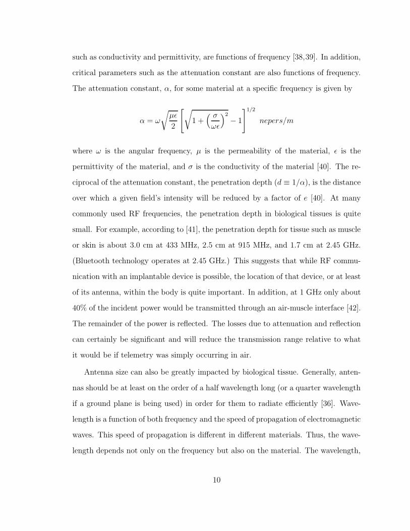
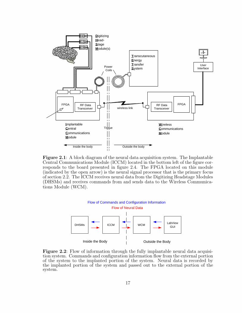
wireless link
Figure 2.1: A block diagram of the neural data acquisition system. The ImplantableCentral Communications Module (ICCM) located in the bottom left of the figure cor-responds to the board presented in figure 2.4. The FPGA located on this module(indicated by the open arrow) is the neural signal processor that is the primary focusof section 2.2. The ICCM receives neural data from the Digitizing Headstage Modules(DHSMs) and receives commands from and sends data to the Wireless Communica-tions Module (WCM).
DHSMs ICCM WCM LabView
GUI
Flow of Commands and Configuration Information
Flow of Neural Data
Outside the Body Inside the Body
Figure 2.2: Flow of information through the fully implantable neural data acquisi-tion system. Commands and configuration information flow from the external portionof the system to the implanted portion of the system. Neural data is recorded bythe implanted portion of the system and passed out to the external portion of thesystem.
17

electrodes connect
here
amplifiers
ADCs
CPLD
Figure 2.3: The digitizing headstage module (DHSM) circuit board. This boardcontains two custom amplifiers, two analog-to-digital converters (ADCs), and a com-plex programmable logic device (CPLD). Neural signals picked up by the electrodesare amplified, filtered, and digitized before being passed on to the Implantable Cen-tral Communications Module (ICCM) for further processing. Each amplifier/ADCpair processes signals from 16 channels. Thus, each DHSM records from a total of32 channels.
18
FPGA
transceiver
Figure 2.4: A circuit board designed for components of a fully implantable moduleof a neural data acquisition system. This board serves as the Implantable CentralCommunications Module (ICCM). The arrows indicate the neural signal processorFPGA and the transceiver with which it interfaces.
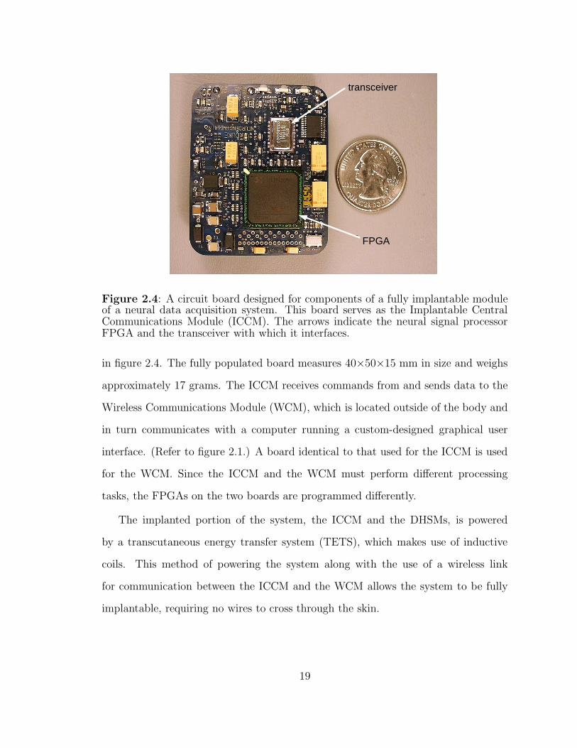
in figure 2.4. The fully populated board measures 40×50×15 mm in size and weighs
approximately 17 grams. The ICCM receives commands from and sends data to the
Wireless Communications Module (WCM), which is located outside of the body and
in turn communicates with a computer running a custom-designed graphical user
interface. (Refer to figure 2.1.) A board identical to that used for the ICCM is used
for the WCM. Since the ICCM and the WCM must perform different processing
tasks, the FPGAs on the two boards are programmed differently.
The implanted portion of the system, the ICCM and the DHSMs, is powered
by a transcutaneous energy transfer system (TETS), which makes use of inductive
coils. This method of powering the system along with the use of a wireless link
for communication between the ICCM and the WCM allows the system to be fully
implantable, requiring no wires to cross through the skin.
19

2.2 Processing Performed by the Implantable Cen-
tral Communications Module
The programmable logic for processing the neural data and interfacing with the
transceiver has been implemented in a Xilinx (San Jose, CA) Virtex-II XC2V1000
FPGA. This implementation has been performed using a combination of the VHDL
and Verilog hardware description languages and consists of more than 50 distinct
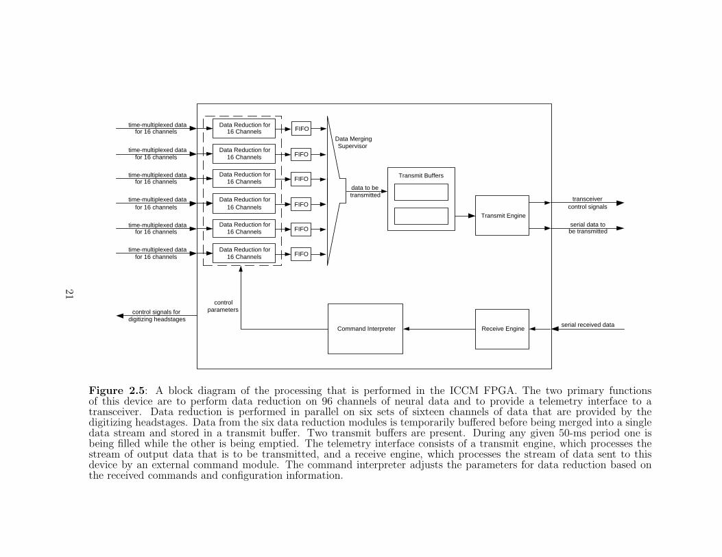
modules. The general organization of this processing is shown in figure 2.5. Data
reduction is applied to each set of sixteen channels independently and simultaneously.
The output from the six data reduction modules is then merged together to form a
single stream of data that can be sent to the transceiver.
2.2.1 Data Reduction
Data reduction is a key function of the neural signal processor. Without data reduc-
tion, and assuming no overhead for telemetry, fewer than three full channels of data
could be transmitted using a 1 Mbps transceiver.
(106 bits/second)/(12 bits/sample)
(31250 samples/second/channel)= 2.67 channels
In order to effectively make use of the 96 channels of input data, data reduction
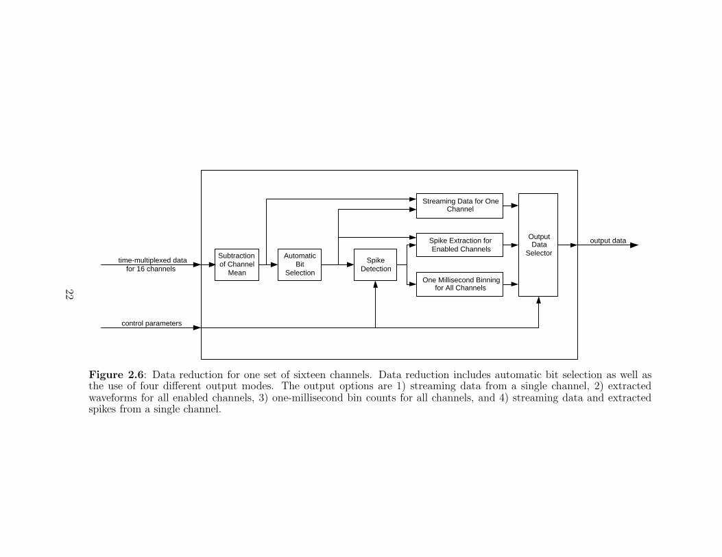
is necessary. Figure 2.6 shows a diagram of the data reduction scheme for sixteen
channels.
Automatic Bit Selection
One effective method of reducing the amount of data is to simply reduce the bit
resolution of the output data. The DHSMs use 12-bit analog-to-digital converters
(ADCs) and pass all twelve bits to the neural signal processor. However, the use
of all twelve bits is generally unnecessary. For low amplitude signals, the highest
20
time-multiplexed data for 16 channels
Data Reduction for 16 Channels
Data Reduction for 16 Channels
Data Reduction for 16 Channels
Data Reduction for 16 Channels
Data Reduction for 16 Channels
Data Reduction for 16 Channels
time-multiplexed data for 16 channels
time-multiplexed data for 16 channels
time-multiplexed data for 16 channels
time-multiplexed data for 16 channels
time-multiplexed data for 16 channels
control signals for digitizing headstages
Transmit Engine
data to be transmitted
Command Interpreter
control parameters
transceiver control signals
serial data to be transmitted
serial received data
FIFO
FIFO
FIFO
FIFO
FIFO
FIFO
Transmit Buffers
Receive Engine
Data Merging Supervisor
Figure 2.5: A block diagram of the processing that is performed in the ICCM FPGA. The two primary functionsof this device are to perform data reduction on 96 channels of neural data and to provide a telemetry interface to atransceiver. Data reduction is performed in parallel on six sets of sixteen channels of data that are provided by thedigitizing headstages. Data from the six data reduction modules is temporarily buffered before being merged into a singledata stream and stored in a transmit buffer. Two transmit buffers are present. During any given 50-ms period one isbeing filled while the other is being emptied. The telemetry interface consists of a transmit engine, which processes thestream of output data that is to be transmitted, and a receive engine, which processes the stream of data sent to thisdevice by an external command module. The command interpreter adjusts the parameters for data reduction based onthe received commands and configuration information.
21
time-multiplexed data for 16 channels
control parameters
Spike Detection
Streaming Data for One Channel
Output Data
Selector
output data
One Millisecond Binning for All Channels
Spike Extraction for Enabled Channels
Automatic Bit
Selection
Subtraction of Channel
Mean
Figure 2.6: Data reduction for one set of sixteen channels. Data reduction includes automatic bit selection as well asthe use of four different output modes. The output options are 1) streaming data from a single channel, 2) extractedwaveforms for all enabled channels, 3) one-millisecond bin counts for all channels, and 4) streaming data and extractedspikes from a single channel.
22
bits contain no information. For high amplitude signals, the resolution provided by
the lowest bits is not critical. These bits can be ignored with minimal loss of useful
information. The neural signal processor performs automatic bit selection to select
the “best” eight bits for each channel. The “best” eight bits are the bits that provide
the highest resolution while still providing sufficient range on a given channel. This
determination is made based on approximately two seconds’ worth of data that are
collected during an initial monitoring period. This monitoring period is initiated by
a Reset command received from the WCM. (The commands are described in section
2.2.3.) The bits are selected to allow for a roughly 25% increase in deviation from the
channel mean over that seen during the monitoring period. Any further processing
within the neural signal processor is then performed on these 8-bit samples. In
addition, the mean value for each channel is computed during the initial monitoring
period. From then on, the mean computed for a given channel is subtracted from
incoming samples on that channel. Consequently, the data to be processed for each
channel is “zero-mean.” Selection of bits for a given sample is made after the mean has
been subtracted. The most significant bit of the 12-bit sample essentially performs
the function of a sign bit, so it is always preserved regardless of which other bits are
selected. Automatic bit selection significantly reduces the amount of data, allows for
a relatively large input range, and retains the resolution of low-amplitude signals.
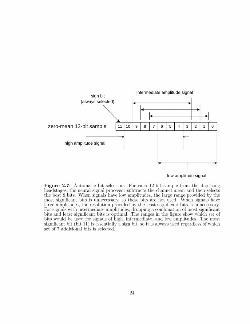
Figure 2.7 illustrates automatic bit selection.
The DHSMs have a voltage gain of 5000, and the ADCs on the DHSMs have a full-
scale range of 2.4 V. Table 2.1 shows the input-referred voltage range and resolution
corresponding to each set of 8 bits that can be chosen during automatic bit selection.
Additionally, the table shows the set of bits that will be selected as a function of the
maximum deviation from the channel mean observed during the monitoring period.
23
intermediate amplitude signal
11 10 9 8 7 6 5 4 3 2 1 0 zero-mean 12-bit sample
low amplitude signal
high amplitude signal
sign bit (always selected)
Figure 2.7: Automatic bit selection. For each 12-bit sample from the digitizingheadstages, the neural signal processor subtracts the channel mean and then selectsthe best 8 bits. When signals have low amplitudes, the large range provided by themost significant bits is unnecessary, so these bits are not used. When signals havelarge amplitudes, the resolution provided by the least significant bits is unnecessary.For signals with intermediate amplitudes, dropping a combination of most significantbits and least significant bits is optimal. The ranges in the figure show which set ofbits would be used for signals of high, intermediate, and low amplitudes. The mostsignificant bit (bit 11) is essentially a sign bit, so it is always used regardless of whichset of 7 additional bits is selected.
24
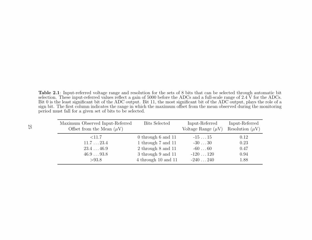
Table 2.1: Input-referred voltage range and resolution for the sets of 8 bits that can be selected through automatic bitselection. These input-referred values reflect a gain of 5000 before the ADCs and a full-scale range of 2.4 V for the ADCs.Bit 0 is the least significant bit of the ADC output. Bit 11, the most significant bit of the ADC output, plays the role of asign bit. The first column indicates the range in which the maximum offset from the mean observed during the monitoringperiod must fall for a given set of bits to be selected.
Maximum Observed Input-Referred Bits Selected Input-Referred Input-ReferredOffset from the Mean (µV) Voltage Range (µV) Resolution (µV)
<11.7 0 through 6 and 11 -15 . . . 15 0.1211.7 . . . 23.4 1 through 7 and 11 -30 . . . 30 0.2323.4 . . . 46.9 2 through 8 and 11 -60 . . . 60 0.4746.9 . . . 93.8 3 through 9 and 11 -120 . . . 120 0.94
>93.8 4 through 10 and 11 -240 . . . 240 1.88
25
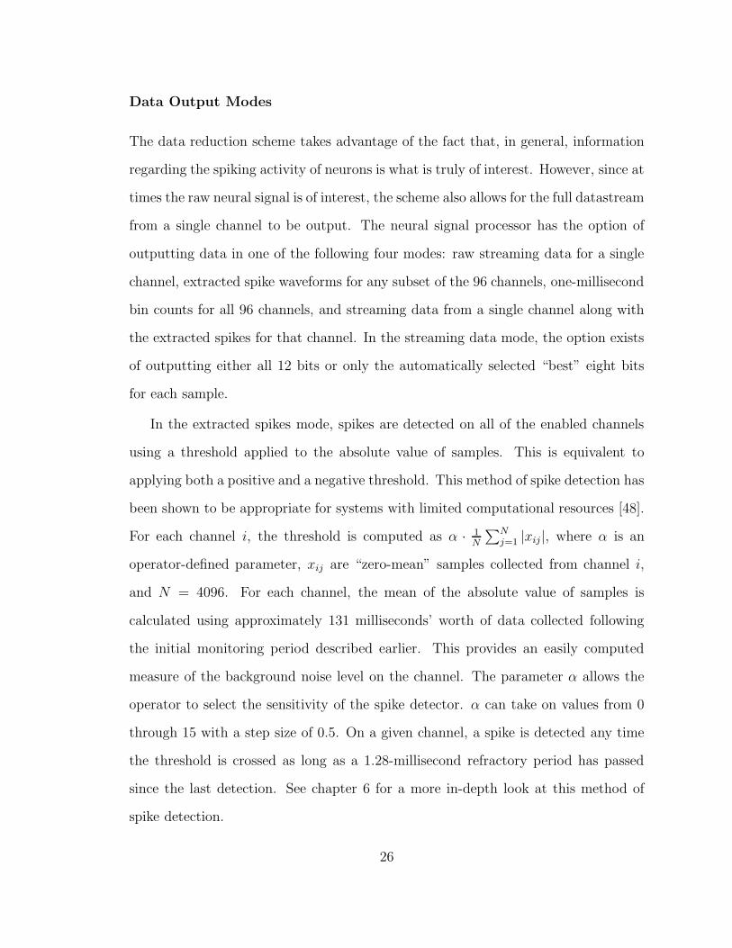
Data Output Modes
The data reduction scheme takes advantage of the fact that, in general, information
regarding the spiking activity of neurons is what is truly of interest. However, since at
times the raw neural signal is of interest, the scheme also allows for the full datastream
from a single channel to be output. The neural signal processor has the option of
outputting data in one of the following four modes: raw streaming data for a single
channel, extracted spike waveforms for any subset of the 96 channels, one-millisecond
bin counts for all 96 channels, and streaming data from a single channel along with
the extracted spikes for that channel. In the streaming data mode, the option exists
of outputting either all 12 bits or only the automatically selected “best” eight bits
for each sample.
In the extracted spikes mode, spikes are detected on all of the enabled channels
using a threshold applied to the absolute value of samples. This is equivalent to
applying both a positive and a negative threshold. This method of spike detection has
been shown to be appropriate for systems with limited computational resources [48].
For each channel i, the threshold is computed as α · 1N
∑Nj=1 |xij|, where α is an
operator-defined parameter, xij are “zero-mean” samples collected from channel i,
and N = 4096. For each channel, the mean of the absolute value of samples is
calculated using approximately 131 milliseconds’ worth of data collected following
the initial monitoring period described earlier. This provides an easily computed
measure of the background noise level on the channel. The parameter α allows the
operator to select the sensitivity of the spike detector. α can take on values from 0
through 15 with a step size of 0.5. On a given channel, a spike is detected any time
the threshold is crossed as long as a 1.28-millisecond refractory period has passed
since the last detection. See chapter 6 for a more in-depth look at this method of
spike detection.
26
For each detected spike, a 48-byte packet is constructed containing the number of
the channel on which the spike occurred, a two-byte timestamp with one-millisecond
resolution, and a 45-byte spike waveform. Thus shape, timing, and channel informa-
tion is included in the output for each detected spike. The timestamp is synchronized
to a timer contained in the external WCM. As a result, the timing of spikes extracted
within the body can be known relative to events occurring outside of the body. Minor
adjustments to the timer in the neural signal processor are made every 50 ms to pre-
vent drift between the internal and external timers. In addition, every four seconds,
the internal timer is set to exactly match the external timer. The spike waveform
includes 10 samples before the threshold crossing and 35 samples after it.
In cases in which the spike shape is not of interest, the data can be reduced even
further by detecting spikes and outputting bin counts for each one-millisecond period.
Since the temporal extent of a neural spike is on the order of one millisecond, each
one-millisecond bin count has a value of either 0 or 1. The fourth output mode,
streaming data with extracted spikes for a single channel, presents both raw and
reduced data for one channel. For each of these modes, the neural signal processor
outputs a packet of data every fifty milliseconds.
Merging of Output Data
As stated earlier, six lines of serial data, each containing data from 16 channels,
serve as input to the neural signal processor. These six lines are processed in parallel
resulting in up to six separate streams of reduced neural data. Only one stream
of data can be sent to the transceiver. Thus, as the data reduction on each of the
individual lines is performed, the output from the six data reduction modules is
merged together to form a single stream of data to be sent to the transceiver.
This merging procedure is trivial in all data output modes except for the extracted
27
spikes mode. In the extracted spikes mode the merging of the data is complicated by
the fact that the amount of data (based on the number of spikes) and the location of
the data (based on the set of 16 channels on which a given spike occurs) cannot be
known beforehand. To deal with this, an extra level of buffering is used to temporarily
hold spikes in each individual sixteen-channel data reduction module until those
spikes can be merged into the single output datastream. Each data reduction module
has its own two-kilobyte first-in-first-out (FIFO) buffer. Each FIFO can hold 42
extracted spikes. As spikes are extracted and placed into these FIFOs, a data merging
supervisor keeps track of the time when spikes are placed into the individual FIFOs
and then reads them out in the proper order. As spikes are read out, the merged
output datastream is stored in a transmit buffer. The system has two transmit buffers
each capable of holding 4800 bytes, which corresponds to exactly 100 extracted spikes.
During a given fifty-millisecond period, one transmit buffer is being filled while the
other is being read out so that its data can be transmitted by the transceiver. At
the end of the fifty-millisecond period, the buffers are switched so that the one that
is now empty can be filled with new data and the one that just finished being filled
can have its data transmitted.
Each transmit buffer has a finite amount of storage space. Before reading a spike
out from a FIFO, the data merging supervisor checks to make sure that the transmit
buffer has space to hold a new spike. If the transmit buffer is full, spikes remain in
the FIFOs until the swap of transmit buffers frees up space to hold more spikes. As a
result, it is possible that a FIFO may fill up and be unable to hold additional spikes.
If spikes are extracted within a data reduction module that has a full FIFO, these
spikes are dropped from the output datastream. With each set of extracted spikes
that is output, the neural signal processor provides an indication for each of the six
data reduction modules of whether or not any spikes had to be dropped from that
28

module during the corresponding fifty-millisecond period.
The FIFOs are also used in the streaming data with extracted spikes mode. In
this mode, data is recorded from a single channel. During a 50-ms period, streaming
data is stored in a transmit buffer and extracted spikes are stored in the FIFO for
the data reduction module which corresponds to the active channel. At the end of
the 50-ms period, the streaming data from that period is sent to the transceiver.
The extracted spikes for that period are then read out of the FIFO and sent to the
transceiver.
2.2.2 Telemetry
A telemetry link provides a means of communication between an implanted portion
of a neural data acquisition system and the external world. Our system requires
information to flow in both directions (see figure 2.2). Commands and configuration
information must be sent from the external world into the implanted portion of the
system, and the recorded neural data must be sent from inside the body out to
the external world. Our bidirectional telemetry link consists of the following three
components: a transceiver, transmit and receive engines within the FPGA in order to
interface with the transceiver, and an antenna with matching network. The external
unit (the WCM) and the implantable unit (the ICCM) have each of these components.
Transceiver
We use a commercial 1 Mbps transceiver with a carrier frequency of 916.5 MHz
(TR1100, RF Monolithics, Inc., Dallas, TX). This transceiver is intended for use in
applications in which low power, short-range wireless communication is needed. The
transceiver uses amplitude-shift keyed modulation. This form of modulation allows
binary data to be transmitted by simply representing a low bit by a low transmitted
29
power level and a high bit by a higher transmitted power level [49].
Transceiver Interface
The transceiver uses a three-line interface. One line determines the transceiver’s
transmit/receive state. Another line serves as the input to the transceiver when in
transmit mode. The third line serves as the output from the transceiver when in
receive mode.
The transmit engine formats the single stream of output data (see section 2.2.1)
so that it can be transmitted successfully over the telemetry link. A packet consisting
of the output data and header information is assembled so that the receiver can both
interpret and perform error-checking on the received data. Each byte is encoded
into a 10-bit symbol (8b/10b encoding [50]) to ensure that the bitstream that is sent
to the transceiver is DC-balanced, to allow for the use of special symbols, and to
ensure that the minimum transition requirements for bit recovery are met. Finally,
the encoded bitstream is sent serially to the transceiver.
The receive engine takes the bitstream that is output from the transceiver and
reconstructs and decodes it. No timing or framing information is received apart from
that which can be extracted from the received serial data stream. When receiving
data, the receive engine first recovers the bitstream present in the received data line
using a data locked loop [51]. Once the individual bits and framing information
have been recovered, 10-bit symbols are decoded and interpreted based on the packet
structure. Finally, the received commands and data are passed out of the receive
engine for further use within the system.
The presence of both a transmit engine and a receive engine provides the capa-
bility for bidirectional communication. The transmit and receive engines are com-
plementary. In other words, the receive engine is designed to properly interpret data
30

that has been processed by the transmit engine. Consequently, both the implantable
module and the external module use these engines to interface with their respective
transceivers.
Matching Network and Antenna
The transceiver is connected to an antenna through a matching network. The match-
ing network has been tuned to match the impedance of the antenna with that of the
transceiver and to facilitate the efficient transfer of power between the transceiver
and antenna. Different types of antennas are used for the WCM and the ICCM. The
ICCM antenna is constrained by the fact that it must be implantable. We primarily
used two designs for the ICCM antenna – a dipole made of floppy, stranded stainless
steel wire and a monopole made by stripping off the appropriate length of shielding
from a coaxial cable. The monopole and each leg of the dipole were 4 cm long. The
latter design was found to be preferable since it was easier to implant.
The WCM antenna essentially has no constraints since it is part of an external
unit. We primarily used a 5-element Yagi antenna (ANT-916-YG5-N, Antenna Fac-
tor, Merlin, OR) or a commercial half wavelength dipole (ANT-916-MHW-RPS-S,
Antenna Factor, Merlin, OR) as the WCM antenna.
2.2.3 Command Interpretation
The neural signal processor is capable of responding to the following five commands
from the WCM: 1) Loopback, 2) Write Configuration Registers, 3) Read Configura-
tion Registers, 4) Request Acquired Data, and 5) Reset. In typical operation, the
ICCM expects to receive a command from the WCM every fifty milliseconds.
The Loopback command is sent by the WCM in a packet along with 256 data
bytes. Upon receiving this packet, the ICCM responds by echoing back the received
31
data. This command is used to ensure that the communication pathway is operating
properly. The Write Configuration Registers command is used to configure settings
within the implantable portion of the system. The packet in which this command is
sent contains information for setting a channel enable list, the data acquisition mode
(one of the four modes described in section 2.2.1), the operator-defined parameter
used in calculating thresholds (α), and additional setting for the DHSMs. In response
to this command, the ICCM updates its internal settings and sends a copy of the
received data back to the WCM. The Read Configuration Registers command allows
the external module to determine the current settings of the neural signal processor.
In response to this command, the ICCM transmits its current configuration settings.
It also sends an indication of which eight bits were selected for each channel during
the automatic bit selection. This information is necessary for mapping the data that
are sent back to the external module into actual voltages. The Request Acquired Data
command is the command that allows the WCM to obtain the neural data that has
been acquired over the past fifty milliseconds. The format of the data output by the
neural signal processor in response to this command is based on the data acquisition
mode setting. The final command, Reset, initiates the calculation of channel means,
automatic bit selection, and the calculation of thresholds.
2.3 Processing Performed by the Wireless Com-
munications Module
The WCM’s primary function is to simply communicate with the ICCM. The WCM
relays commands to the ICCM and receives data from the ICCM so that that data
can be used elsewhere. Depending on the end use of the neural data, the data received
by the WCM may be useful directly in the form in which it is output by the ICCM.
However, in some cases further processing of the data is desirable. Two additional
32
processing steps have been implemented within the WCM – 50-millisecond binning
and real-time spike sorting.
2.3.1 Fifty-Millisecond Binning
The ICCM has the capability of outputting 1-ms bin counts. While this provides
resolution of individual spikes, ultimately it is not the most useful form of binning.
Bin counts are generally used to provide an estimate of instantaneous firing rates.
The temporal duration of a spike is on the order of 1 ms. Thus, 1-ms bin counts are
not very useful in providing an estimate of the instantaneous firing rate. Commonly
used bin widths are on the order of 50 or 100 ms [6, 12, 14]. The WCM has the
capability of compiling the 1-ms bin counts provided by the ICCM into 50-ms bin
counts and outputting these more standard bin counts.
2.3.2 Spike Sorting
The main purpose for providing the ICCM with the ability to extract spike wave-
forms rather than to only detect spikes is to allow for spike sorting. Spike sorting is
commonly performed within BMI and other neural data acquisition applications. It
is generally a computationally intense process. Spike sorting is commonly performed
in a two-phase process: spike templates are generated during a learning phase and
then template matching is performed in a real-time phase. The task of template
matching is computationally suitable for implementation in a fully implantable sys-
tem; however, the process of generating templates is computationally complex and
typically requires supervision. The programmable logic contained in our system is not
well-suited to perform many of the mathematical manipulations (principal compo-
nent analysis, for example) that are often used in generating templates. Commercial
software that provides the functionality and necessary user interactivity to generate
33
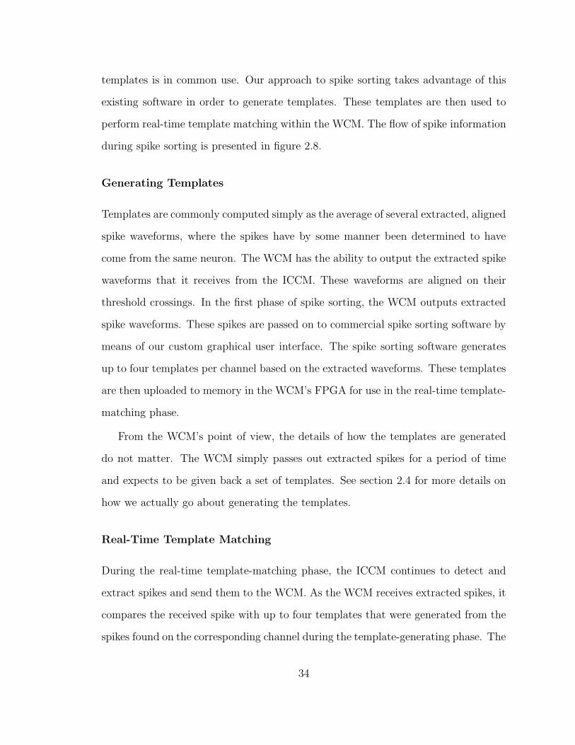
templates is in common use. Our approach to spike sorting takes advantage of this
existing software in order to generate templates. These templates are then used to
perform real-time template matching within the WCM. The flow of spike information
during spike sorting is presented in figure 2.8.
Generating Templates
Templates are commonly computed simply as the average of several extracted, aligned
spike waveforms, where the spikes have by some manner been determined to have
come from the same neuron. The WCM has the ability to output the extracted spike
waveforms that it receives from the ICCM. These waveforms are aligned on their
threshold crossings. In the first phase of spike sorting, the WCM outputs extracted
spike waveforms. These spikes are passed on to commercial spike sorting software by
means of our custom graphical user interface. The spike sorting software generates
up to four templates per channel based on the extracted waveforms. These templates
are then uploaded to memory in the WCM’s FPGA for use in the real-time template-
matching phase.
From the WCM’s point of view, the details of how the templates are generated
do not matter. The WCM simply passes out extracted spikes for a period of time
and expects to be given back a set of templates. See section 2.4 for more details on
how we actually go about generating the templates.
Real-Time Template Matching
During the real-time template-matching phase, the ICCM continues to detect and
extract spikes and send them to the WCM. As the WCM receives extracted spikes, it
compares the received spike with up to four templates that were generated from the
spikes found on the corresponding channel during the template-generating phase. The
34
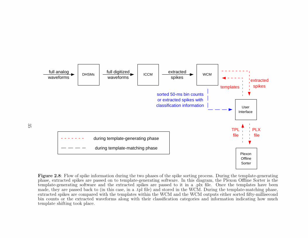
DHSMs full analog waveforms
ICCM full digitized waveforms
WCM extracted
spikes
User Interface
extracted spikes
Plexon Offline Sorter
PLX file
TPL file
templates
sorted 50-ms bin counts or extracted spikes with classification information
during template-generating phase
during template-matching phase
Figure 2.8: Flow of spike information during the two phases of the spike sorting process. During the template-generatingphase, extracted spikes are passed on to template-generating software. In this diagram, the Plexon Offline Sorter is thetemplate-generating software and the extracted spikes are passed to it in a .plx file. Once the templates have beenmade, they are passed back to (in this case, in a .tpl file) and stored in the WCM. During the template-matching phase,extracted spikes are compared with the templates within the WCM and the WCM outputs either sorted fifty-millisecondbin counts or the extracted waveforms along with their classification categories and information indicating how muchtemplate shifting took place.
35

sum of squared errors (SSE) between the extracted spike and each of the applicable
templates is computed. Each template is also shifted one and two samples (32 µs per
sample) in each direction in order to reduce errors due to alignment issues. A spike is
classified as matching the template that either in its original form or a shifted form
results in the minimum SSE as long as the computed SSE is below a specified value.
Based on these classifications, the WCM generates 50-ms bin counts for each unit.
These 384 bin counts (4 units/channel ∗ 96 channels = 384 units) are sent out of
the WCM every 50 milliseconds. In addition a count for an “unclassified” category
is generated and output for each channel. A spike is placed into this category if no
templates have been stored for the channel from which the spike was extracted or if
the spike does not sufficiently match (based on the SSE metric) any of the applicable
templates. Finally, the option exists to output each individual extracted waveform
along with its classification category and an indication of the amount of template
shifting that was found to be optimal.
2.4 Graphical User Interface
We have developed a LabView graphical user interface (GUI) to serve as a link
between a user and the WCM. The WCM interfaces to a digital I/O data acquisition
card (653X, National Instruments, Austin, TX) installed in the computer running the
GUI. A user can view and store data output from the WCM through this interface.
This also provides a means by which commands and configuration information can
be sent to the WCM and ultimately to the ICCM.
Most of the processing performed by the GUI simply assists the user in properly
interpreting the data. For example, the neural data output by the WCM must be
scaled appropriately in order to be displayed in microvolts. The scaling depends on
which bits were selected during the automatic bit selection procedure and may differ
36
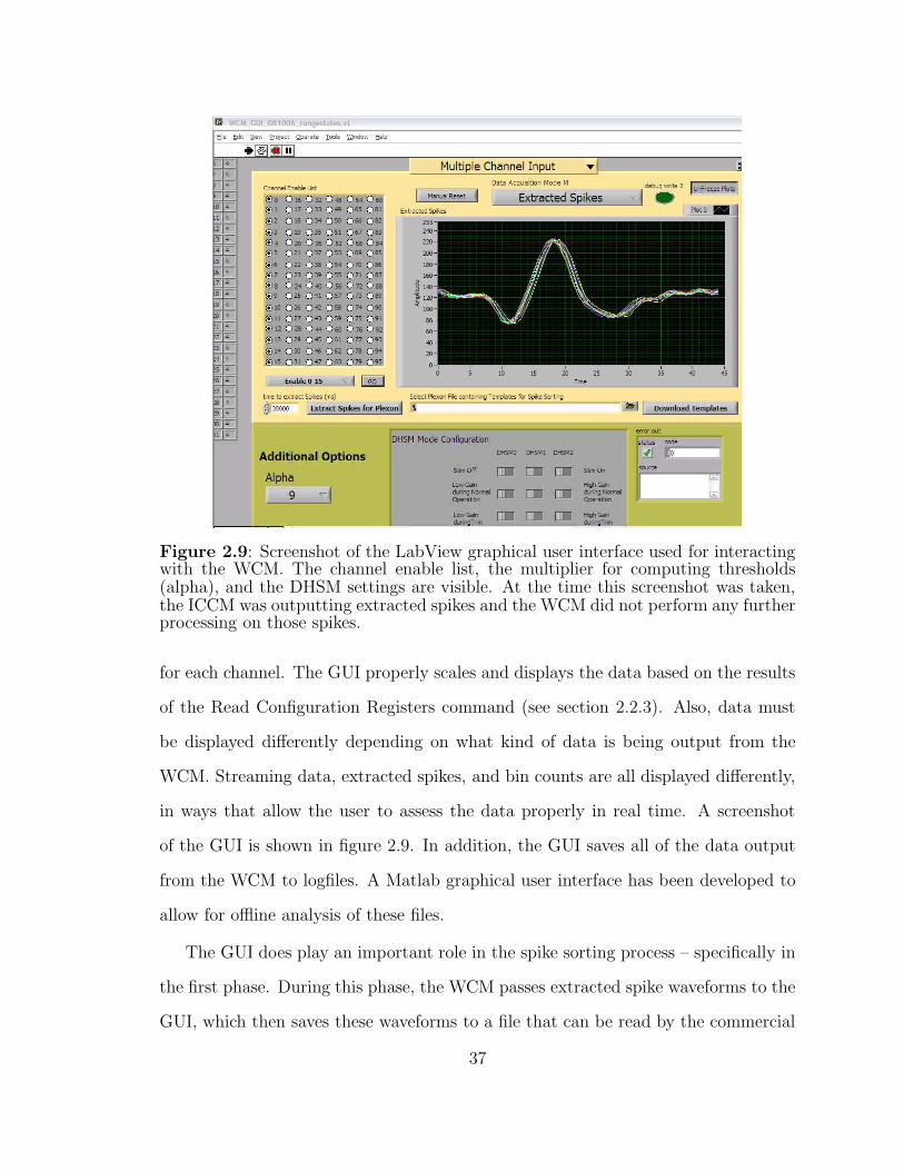
Figure 2.9: Screenshot of the LabView graphical user interface used for interactingwith the WCM. The channel enable list, the multiplier for computing thresholds(alpha), and the DHSM settings are visible. At the time this screenshot was taken,the ICCM was outputting extracted spikes and the WCM did not perform any furtherprocessing on those spikes.
for each channel. The GUI properly scales and displays the data based on the results
of the Read Configuration Registers command (see section 2.2.3). Also, data must
be displayed differently depending on what kind of data is being output from the
WCM. Streaming data, extracted spikes, and bin counts are all displayed differently,
in ways that allow the user to assess the data properly in real time. A screenshot
of the GUI is shown in figure 2.9. In addition, the GUI saves all of the data output
from the WCM to logfiles. A Matlab graphical user interface has been developed to
allow for offline analysis of these files.
The GUI does play an important role in the spike sorting process – specifically in
the first phase. During this phase, the WCM passes extracted spike waveforms to the
GUI, which then saves these waveforms to a file that can be read by the commercial
37

spike sorting software. We use the Plexon (Dallas, TX) Offline Sorter software. The
extracted spikes are saved in the .plx file format. The user then utilizes the features
and functionality of the Offline Sorter to generate templates. This would typically
involve having Offline Sorter map each waveform to a point in principal component
space followed by a user manually drawing circles around distinct clusters of points
within the space. Once all of the spikes have been classified, templates are computed
as the average of all of the spikes within a cluster. The templates are saved in Plexon’s
.tpl file format and the GUI uploads them to memory in the WCM’s FPGA.
38

Chapter 3
System Evaluation
This chapter presents the results of testing various aspects of the fully implantable
neural data acquisition system. This evaluation focuses primarily on the processing
performed within the system but touches on other aspects of the system as well.
3.1 Neural Signal Simulator
In order to evaluate the performance of the system’s spike processing, known data
must be used as input. We developed a neural signal simulator to provide input to
our system. The simulator is made up of two main components – an analog output
card and an attenuator board. We use a National Instruments 6723 analog output
card to output up to 32 analog waveforms. The waveforms may either be read in
from a file and then output through the analog output card repeatedly (i.e., restarting
from the beginning once the waveforms reach their ends), or they may be generated
in real-time by a LabView application running on the computer in which the analog
output card is installed.
The 32 analog waveforms are then passed to the attenuator board, which is shown
in figure 3.1. The attenuator board reduces the amplitude of the signals by a factor of
10000. This results in signals within the physiological range of extracellular potentials
(on the order of tens or hundreds of microvolts). The attenuator board also has an
output impedance similar to that of microelectrodes (on the order of a few hundred
kilohms). Finally, the attenuator board maps the 32 input channels from the analog
output card to 96 output channels that can serve as input into our neural data
acquisition system. Several of the 32 simulated waveforms are mapped to multiple
39
A
B
C
Figure 3.1: Attenuator board for neural signal simulator. Simulated neural wave-forms are output from an analog output card and passed into this board. The signalspass through resistor networks to attenuate the voltage by a factor of 10000. Thesignals can then be fed into the DHSMs. (A) Connectors to input signals from theanalog output card. (B) 32 resistor networks used to attenuate voltage. (C) Connec-tors into which DHSMs can be plugged.
channels, but each set of 16 channels contains 3 channels that are not used elsewhere.
This allows unique sets of signals to be input onto each set of 16 channels.
The key advantage of using the simulator for testing and characterization of the
system’s spike processing is that the simulated waveforms are fully customizable. As
a result, information indicating the timing and unit classification of all “true spikes”
in those waveforms can be known. Thus, unlike live animal recordings, a standard
exists with which to compare the results of the spike processing system.
40
3.2 ICCM Neural Signal Processing
3.2.1 FPGA Utilization and Power Consumption
The VHDL and Verilog hardware description of the ICCM FPGA consists of ap-
proximately 6000 lines of code. The design utilizes almost all of the resources of the
FPGA. Specifically, 49% of the FPGA’s 10240 flip-flops, 93% of the FPGA’s 10240
4-input look-up-tables, and 100% of the FPGA’s 40 18-kilobit blocks of RAM are
used by the design.
The FPGA consumes approximately 100 mW of power. It uses 53 mA from a
1.5 V supply and 7.6 mA from a 3.3 V supply. Each sixteen-channel data reduction
module is responsible for approximately 10 mW of power consumption. The data
merging, telemetry processing, command interpretation, and system supervision have
a combined consumption of about 20 mW. Additionally, the FPGA has a quiescent
power consumption of roughly 20 mW, bringing the total power consumed to 100
mW.
3.2.2 Automatic Bit Selection
In order to test the automatic bit selection feature of the neural signal processor,
we used the neural signal simulator to generate waveforms with spikes of varying
amplitudes. One period of a 2 kHz sine wave with a 180◦ phase-shift was used as
the spike waveform. The spikes occurred at a rate of 20 times per second. No noise
was incorporated into these waveforms. Each waveform was used as input to a single
channel of a DHSM. The neural signal processor performed automatic bit selection
on each waveform. Table 3.1 shows which bits were selected for waveforms with
different spike amplitudes. Spike amplitudes were increased in steps of 10 µV. The
table shows the results for spike amplitudes at the boundaries for the various sets of
41

Table 3.1: Bits selected for waveforms with spikes of various peak amplitudes.
Spike Amplitude (µV) Bits Selected
0 2 through 8 and 1120 2 through 8 and 1130 3 through 9 and 1170 3 through 9 and 1180 4 through 10 and 11
bits. The two lowest sets of bits, bits 0 through 6 and bits 1 through 7, were never
selected due to noise and distortions added to the waveforms by the attenuator board
and recording circuitry. Discrepancies between the results shown in Table 3.1 and
the first two columns of Table 2.1 are also due to the noise and distortions added by
the attenuator board and recording circuitry.
3.2.3 Spike Detection
We evaluated our system’s spike detection performance over a wide range of signal-to-
noise ratios (SNRs). Spike detection was performed using thresholds computed based
on each of thirty different multipliers for each SNR. The spike detection performance
of our system was then compared with the performance of offline spike detection
performed on the waveform seen by the neural signal processor and on the original
input waveform.
We constructed waveforms by first selecting a 2-second noise waveform from a
cortical microelectrode recording made by our system from a rat. This segment was
classified as noise based on the fact that it had no visible spikes. We also created
a spike template, which was simply the average of similarly shaped spikes extracted
from a single channel. Next we randomly selected 40 spike times at which to add a
copy of the template to the 2-second noise waveform. Spikes were placed no closer
than 1.6 ms from each other. We constructed fifteen waveforms. They had SNRs
42

ranging from 1 through 15. Each of these fifteen waveforms used the same noise
waveform, spike template, and spike times. They differed only in the scaling of the
spike template. We define SNR as
SNR =peak amplitude of scaled template
standard deviation of 2-second noise waveform
The waveforms used here are the same as the ones used in section 6.2.4.
Each of the fifteen waveforms was passed through the neural signal simulator into
our neural data acquisition system once for each of the thirty different multipliers.
We used multiplier (i.e., alpha) values from 0.5 through 15 with steps of 0.5. For each
combination of SNR and multiplier, the ICCM was given a Reset command causing
it to compute thresholds at a random point in time within the 2-second waveform.
The ICCM was put into the streaming data with extracted spikes data acquisition
mode. Spike detection performance was then evaluated based on two parameters –
the probability of detection (PD) and the rate of false alarms (RFA). The probability
of detection is defined as
PD =Ncorrect
actual number of spikes in the waveform
and the rate of false alarms is defined as
RFA =total number of detections − Ncorrect
temporal duration of waveform
where Ncorrect is the number of correctly detected spikes. Note that while PD is
unitless, RFA has units of false alarms per second.
Spike detection performance was evaluated for the following three circumstances:
(1) spike detection as performed by the ICCM’s neural signal processor, (2) spike
detection as performed by a Matlab program on the waveform seen by the ICCM’s
43
neural signal processor, and (3) spike detection as performed by a Matlab program
on the original input waveform.
The neural signal processor’s performance was computed based on comparing
the timestamps of the extracted spikes to the known true spike times. (Remember
that the true spike times are known because the spike times were chosen during
the process of constructing the simulated waveforms.) Making this comparison is
complicated by the fact that an unknown offset exists between the reference time
for the timestamp (i.e., the time at which the timestamp has a value of zero) and
the reference time for the true spike times. We addressed this problem by feeding
a waveform that consisted of a single synchronization pulse at the beginning of the
2-second period into a different channel of the neural data acquisition system. The
timestamp of the extraction of this pulse was then used as the reference time for
timestamps. Detections made within 1.5 ms of a true spike time were counted as
true detections. Otherwise, detections were counted as false positives. Since the
neural signal processor’s timestamp has a resolution of 1 ms, we added 0.5 ms to
each timestamp before making the comparisons to the true spike times. This was
done because a spike whose detection time t fell in the range i ≤ t < i + 1 for an
integer i would have a timestamp of i.
The waveform seen by the neural signal processor was known because the ICCM’s
data acquisition mode was streaming data with extracted spikes. Spike detection was
performed offline on the streaming data using a threshold computed as alpha times
the mean of the absolute value of the entire 2-second streaming waveform. Note
that since the neural signal processor computes its threshold based on a randomly
selected 4096-sample window, the thresholds used in these two circumstances will
not be exactly the same. We had to align the waveform seen by the neural signal
processor with the original input waveform so that comparisons between detection
44
times and the true spike times would be meaningful. This was done by finding the
sample within the streaming data that corresponded to a particular timestamp value
assigned during an extraction. The offset in timestamp values was then taken care
of through the use of the synchronization pulse as described above. This procedure
results in knowledge of which sample in the waveform seen by the ICCM corresponds
to which sample in the input waveform. This alignment procedure can be seen to
work well by noting that the waveform in figure 3.3(a) is aligned properly with respect
to the waveform in figure 3.3(b). Once alignment was completed, detections within
1.5 ms of a true spike time were counted as true detections, and other detections were
considered to be false positives.
Finally, spike detection was also performed on the original input waveform (i.e.,
the waveform used as input to the neural signal simulator). Note that this waveform
does not exactly match that seen by the neural signal processor since the act of passing
the signal through the neural signal simulator and the DHSMs affects the signal. Spike
detection in this circumstance was again performed using a threshold computed as
alpha times the mean of the absolute value of the entire 2-second waveform. Once
again, detections were considered to be true detections if and only if they occurred
within 1.5 ms of a true spike time.
Figures 3.2(a) and 3.3(a) show examples of waveforms seen by the neural signal
processor along with the times at which spikes were detected by the neural signal
processor, the times at which spikes were detected by the offline spike detection,
and the true spike times. Figures 3.2(b) and 3.3(b) show examples of original input
waveforms along with the times at which spikes were detected by the offline spike
detection and the true spike times. Figure 3.4 shows, for each SNR, the probability of
detection and the rate of false alarms computed for each of the three circumstances as
a function of the multiplier value. Figure 3.5 shows receiver operating characteristic
45
(ROC) curves for each of the three circumstances for each SNR. In these curves we
plot PD versus RFA. (For more on ROC curves, see section 6.4.7.)
3.2.4 Spike Extraction
In order to investigate the circumstances under which the neural signal processor will
drop extracted spikes from the output datastream, we examined the effect of firing
rate and the distribution of enabled channels on when a data reduction module’s
FIFO would overflow. In each trial, either 16 or 32 channels were enabled. The
following three channel distributions were used: 1) 16 channels enabled – all 16
channels belonging to the same data reduction module; 2) 16 channels enabled – 8
channels belonging to one data reduction module and the other 8 channels belonging
to a different data reduction module; and 3) 32 channels enabled – 16 channels
belonging to one data reduction module and the other 16 channels belonging to a
different data reduction module. For each trial, one of these channel distributions
was selected and a per-channel firing rate was selected. Based on this firing rate,
waveforms were generated with equal spacing between the spikes and provided as
input to our system using the neural signal simulator. For a given trial, identical
waveforms were used as input to all of the enabled channels.
When 16 channels all belonging to the same data reduction module were enabled,
spikes were first dropped at a firing rate of 126 spikes per second per channel. When
16 channels evenly split between two data reduction modules were enabled, spikes
were also first dropped at a firing rate of 126 spikes per second per channel. In both
of these cases, no FIFO overflow was observed at a firing rate of 125 spikes per second
per channel. Also, in both cases at a firing rate of 126 spikes per second per channel,
roughly 20% of the packets indicated that spikes were dropped. At a firing rate of
130 spikes per second per channel, generally every other packet indicated dropped
46
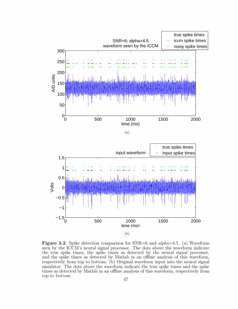
0 500 1000 1500 20000
50
100
150
200
250
300A
/D u
nits
time (ms)
SNR=6; alpha=4.5waveform seen by the ICCM
true spike timesiccm spike timesnoisy spike times
(a)
0 500 1000 1500 2000−1.5
−1
−0.5
0
0.5
1
1.5
Vol
ts
time (ms)
input waveform
true spike timesinput spike times
(b)
Figure 3.2: Spike detection comparison for SNR=6 and alpha=4.5. (a) Waveformseen by the ICCM’s neural signal processor. The dots above the waveform indicatethe true spike times, the spike times as detected by the neural signal processor,and the spike times as detected by Matlab in an offline analysis of this waveform,respectively from top to bottom. (b) Original waveform input into the neural signalsimulator. The dots above the waveform indicate the true spike times and the spiketimes as detected by Matlab in an offline analysis of this waveform, respectively fromtop to bottom.
47
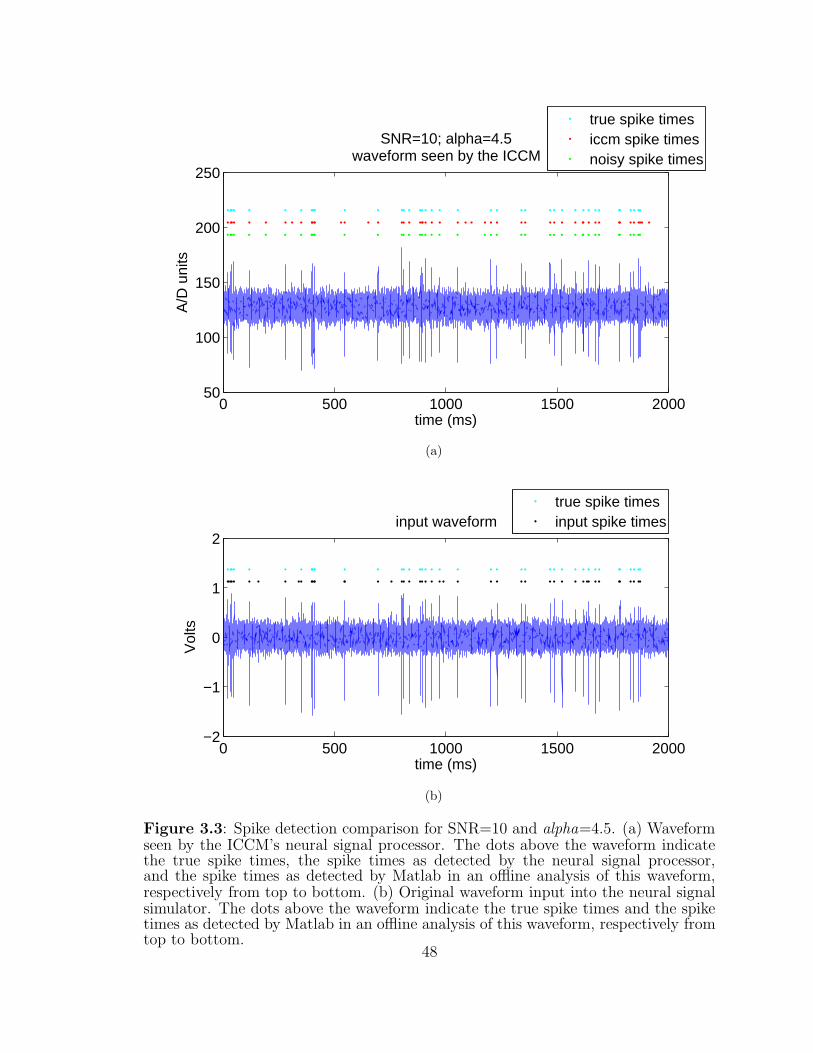
0 500 1000 1500 200050
100
150
200
250A
/D u
nits
time (ms)
SNR=10; alpha=4.5waveform seen by the ICCM
true spike timesiccm spike timesnoisy spike times
(a)
0 500 1000 1500 2000−2
−1
0
1
2
Vol
ts
time (ms)
input waveform
true spike timesinput spike times
(b)
Figure 3.3: Spike detection comparison for SNR=10 and alpha=4.5. (a) Waveformseen by the ICCM’s neural signal processor. The dots above the waveform indicatethe true spike times, the spike times as detected by the neural signal processor,and the spike times as detected by Matlab in an offline analysis of this waveform,respectively from top to bottom. (b) Original waveform input into the neural signalsimulator. The dots above the waveform indicate the true spike times and the spiketimes as detected by Matlab in an offline analysis of this waveform, respectively fromtop to bottom.
48

0 5 10 150
0.5
1SNR=1
PD
0 5 10 150
500
1000
RF
A
0 5 10 150
0.5
1SNR=2
0 5 10 150
500
1000
0 5 10 150
0.5
1SNR=3
0 5 10 150
500
1000
0 5 10 150
0.5
1SNR=4
0 5 10 150
500
1000
0 5 10 150
0.5
1SNR=5
0 5 10 150
500
1000
0 5 10 150
0.5
1SNR=6
PD
0 5 10 150
500
1000
RF
A
0 5 10 150
0.5
1SNR=7
0 5 10 150
500
1000
0 5 10 150
0.5
1SNR=8
0 5 10 150
500
1000
0 5 10 150
0.5
1SNR=9
0 5 10 150
500
1000
0 5 10 150
0.5
1SNR=10
0 5 10 150
500
1000
0 5 10 150
0.5
1SNR=11
PD
0 5 10 150
500
1000
RF
A
alpha
0 5 10 150
0.5
1SNR=12
0 5 10 150
500
1000
alpha
0 5 10 150
0.5
1SNR=13
0 5 10 150
500
1000
alpha
0 5 10 150
0.5
1SNR=14
0 5 10 150
500
1000
alpha
0 5 10 150
0.5
1SNR=15
0 5 10 150
500
1000
alpha
iccm
noisy
input
Figure 3.4: Probability of detection (PD) and rate of false alarms (RFA) as a function of threshold multiplier value(alpha). Spike detection performance on simulated waveforms with SNRs from 1 through 15 is shown. The plots show acomparison of spike detection as performed by our system (iccm), as performed by Matlab on the waveform seen by theICCM (noisy), and as performed by Matlab on the original simulated waveform (input).
49
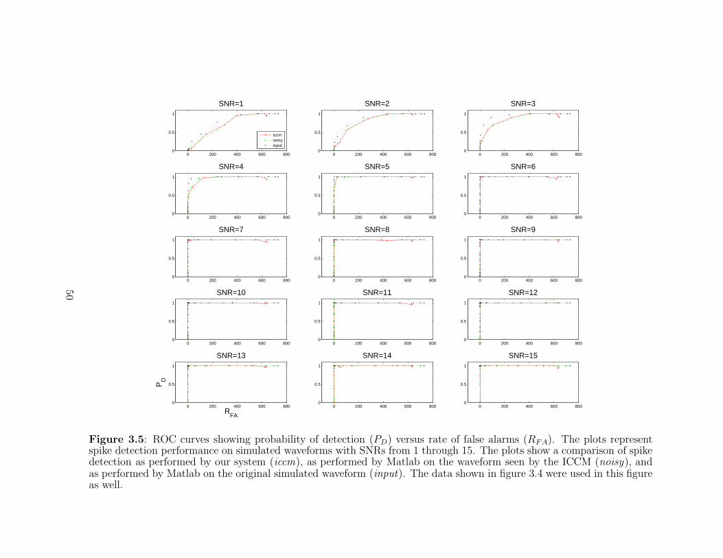
0 200 400 600 8000
0.5
1
SNR=1
0 200 400 600 8000
0.5
1
SNR=2
0 200 400 600 8000
0.5
1
SNR=3
0 200 400 600 8000
0.5
1
SNR=4
0 200 400 600 8000
0.5
1
SNR=5
0 200 400 600 8000
0.5
1
SNR=6
0 200 400 600 8000
0.5
1
SNR=7
0 200 400 600 8000
0.5
1
SNR=8
0 200 400 600 8000
0.5
1
SNR=9
0 200 400 600 8000
0.5
1
SNR=10
0 200 400 600 8000
0.5
1
SNR=11
0 200 400 600 8000
0.5
1
SNR=12
0 200 400 600 8000
0.5
1
SNR=13
RFA
PD
0 200 400 600 8000
0.5
1
SNR=14
0 200 400 600 8000
0.5
1
SNR=15
iccmnoisyinput
Figure 3.5: ROC curves showing probability of detection (PD) versus rate of false alarms (RFA). The plots representspike detection performance on simulated waveforms with SNRs from 1 through 15. The plots show a comparison of spikedetection as performed by our system (iccm), as performed by Matlab on the waveform seen by the ICCM (noisy), andas performed by Matlab on the original simulated waveform (input). The data shown in figure 3.4 were used in this figureas well.
50
spikes.
In the case of 32 enabled channels, spikes were first dropped at a firing rate of 63
spikes per second per channel. Approximately 15% of packets indicated that spikes
were dropped. In this case, no FIFO overflow was observed at a firing rate of 62
spikes per second per channel. At a firing rate of 65 spikes per second per channel,
generally every fourth packet indicated dropped spikes.
3.2.5 Latency
We explored the latencies present in our system between when a spike occurs and
when the corresponding extracted spike is received and is ready for further use within
the WCM. We examined how these latencies behave as the overall firing rate of the
input channels changes. A waveform with a firing rate of approximately one spike
per second was used as input on a “target channel.” The latency was computed as
the time between when the analog output card generated a spike for this channel and
when a spike from this channel was received and ready for further processing within
the WCM. Four different trials were run, each with different overall firing rates. In
each trial, the latencies for 500 spikes were measured. Spikes that were generated
but were never received by the WCM were considered to be dropped spikes.
In each trial, 25 channels in addition to the target channel were enabled. Twelve
of these channels belonged to the same data reduction module as the target channel
and the other 13 channels belonged to a different data reduction module. In the first
trial, the target channel was the only channel with spikes. The mean latency was
26.7 ms. A histogram of the latencies for this case is shown in figure 3.6(a). In the
second trial, each of the 25 enabled non-target channels had a firing rate of 40 spikes
per second, for an overall firing rate of approximately 1000 spikes per second, or 50
spikes per 50 ms. The mean latency was 51.0 ms. The histogram for this case is
51

shown in figure 3.6(b). In the third trial, each of the 25 enabled non-target channels
had a firing rate of 79 spikes per second, for an overall firing rate of just under 2000
spikes per second, or 100 spikes per 50 ms. The mean latency was 74.9 ms and the
histogram is shown in figure 3.6(c). No spikes were dropped in these first three cases.
In the final trial, each of the 25 enabled non-target channels had a firing rate of 85
spikes per second, for an overall firing rate of approximately 2125 spikes per second.
The mean latency was 120.3 ms and 20 out of the 500 spikes were dropped. The
histogram for this case is shown in figure 3.6(d).
3.3 Timestamp Synchronization
It is often desirable to align neural data with other simultaneously recorded data (po-
sition or velocity data, for example) so that temporal correlations and relationships
between the two sets of data can be investigated. With percutaneous, wired neural
data acquisition systems, this can be achieved relatively easily by feeding the analog
neural data and other analog data into a single processing unit that can then sample
all of the individual lines of data. This type of setup makes aligning the two sets of
data trivial since the relationship between when different lines are sampled is known.
The alignment process is more difficult for a fully implantable system due to the fact
that the neural data are sampled by one processor inside the body and external data
must be sampled by a different processor outside the body.
As mentioned in section 2.2.1, the ICCM’s neural signal processor provides a
timestamp with each extracted spike. This timestamp is synchronized to a timer in
the WCM. The WCM’s timer is accessible to the outside world and can consequently
be used to align data collected externally with the spikes extracted internally. Figure
3.7 shows that the WCM and ICCM timestamps are well synchronized. The ICCM
timestamp increments approximately 12µs after the WCM timestamp increments.
52
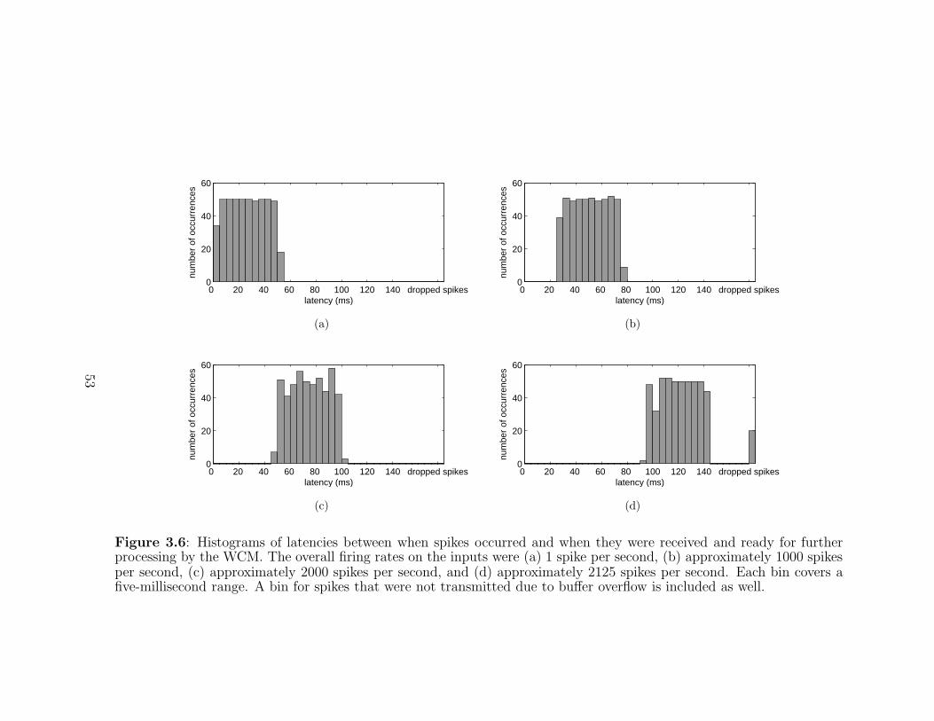
0 20 40 60 80 100 120 140 dropped spikes0
20
40
60
latency (ms)
num
ber
of o
ccur
renc
es
(a)
0 20 40 60 80 100 120 140 dropped spikes0
20
40
60
latency (ms)
num
ber
of o
ccur
renc
es
(b)
0 20 40 60 80 100 120 140 dropped spikes0
20
40
60
latency (ms)
num
ber
of o
ccur
renc
es
(c)
0 20 40 60 80 100 120 140 dropped spikes0
20
40
60
latency (ms)
num
ber
of o
ccur
renc
es(d)
Figure 3.6: Histograms of latencies between when spikes occurred and when they were received and ready for furtherprocessing by the WCM. The overall firing rates on the inputs were (a) 1 spike per second, (b) approximately 1000 spikesper second, (c) approximately 2000 spikes per second, and (d) approximately 2125 spikes per second. Each bin covers afive-millisecond range. A bin for spikes that were not transmitted due to buffer overflow is included as well.
53
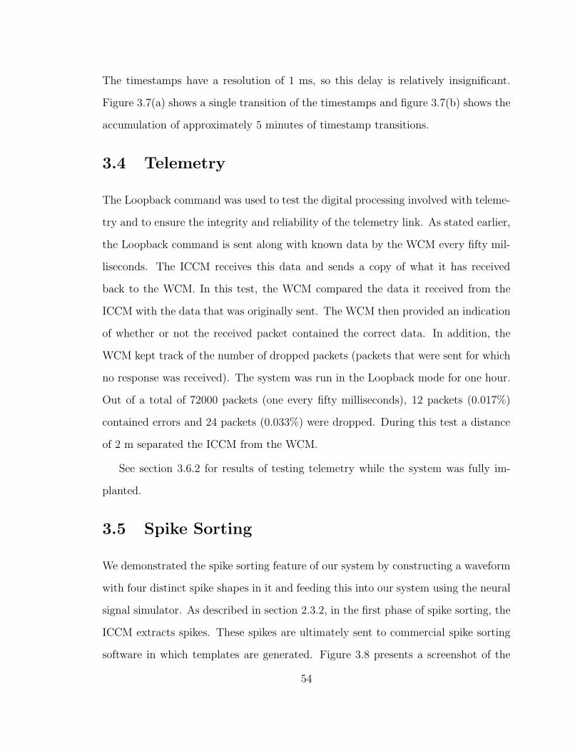
The timestamps have a resolution of 1 ms, so this delay is relatively insignificant.
Figure 3.7(a) shows a single transition of the timestamps and figure 3.7(b) shows the
accumulation of approximately 5 minutes of timestamp transitions.
3.4 Telemetry
The Loopback command was used to test the digital processing involved with teleme-
try and to ensure the integrity and reliability of the telemetry link. As stated earlier,
the Loopback command is sent along with known data by the WCM every fifty mil-
liseconds. The ICCM receives this data and sends a copy of what it has received
back to the WCM. In this test, the WCM compared the data it received from the
ICCM with the data that was originally sent. The WCM then provided an indication
of whether or not the received packet contained the correct data. In addition, the
WCM kept track of the number of dropped packets (packets that were sent for which
no response was received). The system was run in the Loopback mode for one hour.
Out of a total of 72000 packets (one every fifty milliseconds), 12 packets (0.017%)
contained errors and 24 packets (0.033%) were dropped. During this test a distance
of 2 m separated the ICCM from the WCM.
See section 3.6.2 for results of testing telemetry while the system was fully im-
planted.
3.5 Spike Sorting
We demonstrated the spike sorting feature of our system by constructing a waveform
with four distinct spike shapes in it and feeding this into our system using the neural
signal simulator. As described in section 2.3.2, in the first phase of spike sorting, the
ICCM extracts spikes. These spikes are ultimately sent to commercial spike sorting
software in which templates are generated. Figure 3.8 presents a screenshot of the
54
(a)
(b)
Figure 3.7: Synchronization of ICCM and WCM timestamps. (a) Screenshot from alogic analyzer showing the ICCM timestamp (ICCMTS) incrementing approximately12 µs after the WCM timestamp (WCMTS) increments. The filled arrow points tothe time at which the WCM timestamp increments and the open arrow points tothe time at which the ICCM timestamp increments. (b) Screenshot from the logicanalyzer showing that the ICCM timestamp consistently increments approximately12 µs after the WCM timestamp increments. This figure shows the accumulation ofapproximately 5 minutes of timestamp transitions. Again, the filled arrow points tothe time at which the WCM timestamp incremented (the event on which the logicanalyzer was triggered) and the open arrow points to the range of times over whichthe ICCM timestamp incremented during the 5-minute period.
55

Table 3.2: For a given SNR, percentage of spikes for which a given amount oftemplate shifting resulted in the minimum sum of squared errors.
SNR13 10 7 5
shift left 2 samples 0 0 2 4shift left 1 sample 11 9 16 12
no shift 77 77 67 48shift right 1 sample 12 14 14 33shift right 2 samples 0 0 < 1 3
spike sorting software after clustering has been performed. Figure 3.9 shows the
results of the real-time template-matching phase after the templates from figure 3.8
were uploaded into the WCM.
As mentioned in section 2.3.2, the WCM attempts to match incoming extracted
spikes with shifted versions of the templates in addition to the original templates.
Tables 3.2 and 3.3 provide some insight into the effect of shifting templates. For
each of four different SNRs, we simulated spikes, generated templates, and then
had the WCM perform template matching on approximately 200 to 300 spikes. The
extracted spikes are shown in figure 3.10. Table 3.2 shows for each SNR the percentage
of extracted spikes for which a given amount of template shifting resulted in the
minimum SSE. Table 3.3 provides a comparison of the optimal SSEs achieved using
template shifting and the SSEs that would have been obtained if no template shifting
had taken place. Finally, table 3.4 gives a feel for the SSEs that result from comparing
spikes of one size to templates of another size. This table presents the SSEs when
the templates of the four SNRs are compared against each other.
3.6 Live Animal Recordings
The system evaluation presented so far in this chapter has involved testing our system
on the bench. As mentioned in section 3.1, this type of testing is critical because it
56
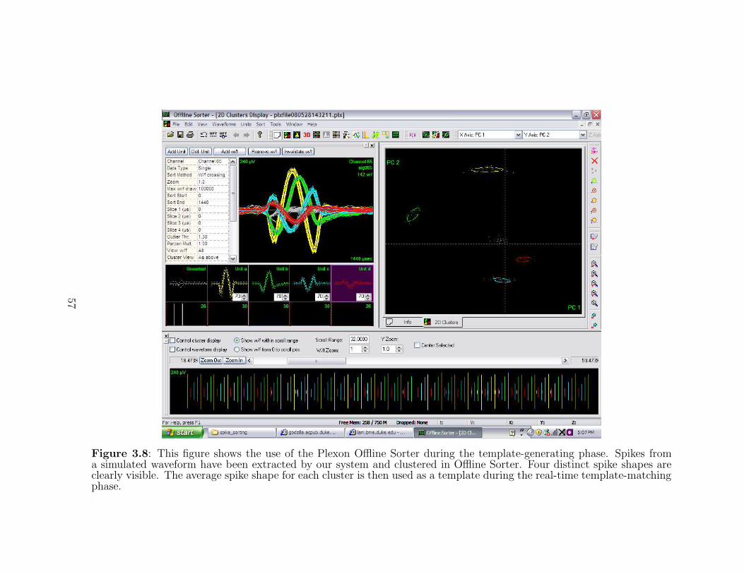
Figure 3.8: This figure shows the use of the Plexon Offline Sorter during the template-generating phase. Spikes froma simulated waveform have been extracted by our system and clustered in Offline Sorter. Four distinct spike shapes areclearly visible. The average spike shape for each cluster is then used as a template during the real-time template-matchingphase.
57
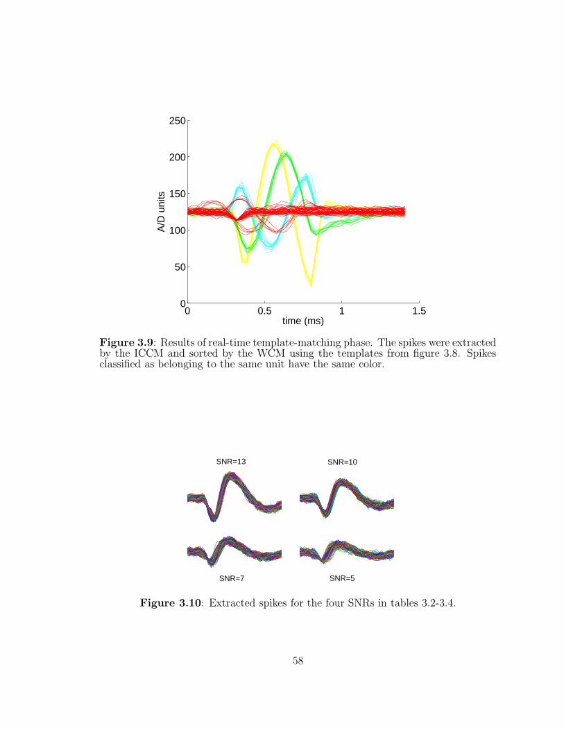
0 0.5 1 1.50
50
100
150
200
250
time (ms)
A/D
uni
ts
Figure 3.9: Results of real-time template-matching phase. The spikes were extractedby the ICCM and sorted by the WCM using the templates from figure 3.8. Spikesclassified as belonging to the same unit have the same color.
SNR=13
SNR=5
SNR=10
SNR=7
Figure 3.10: Extracted spikes for the four SNRs in tables 3.2-3.4.
58

Table 3.3: Mean sum of squared errors (SSE) for spikes that led to a given amountof template shifting. For each SNR, the numbers on the left give the mean SSEbetween the spikes and the non-shifted template. The numbers in parentheses on theright give the mean SSE between the spikes and the optimally shifted template. Theunits are 103 µV 2. A dash (–) indicates that no spikes with a particular SNR led toa given amount of template shifting.
SNR13 10 7 5
shift left 2 samples – (–) – (–) 18 (5) 13 (6)shift left 1 sample 14 (7) 9 (5) 7 (4) 8 (6)
no shift 6 (6) 5 (5) 4 (4) 5 (5)shift right 1 sample 12 (6) 12 (6) 7 (5) 7 (5)shift right 2 samples – (–) – (–) 18 (5) 17 (7)
Table 3.4: Sum of squared errors between pairs of templates. Again, the units are103 µV 2.
template for SNR13 10 7 5
template for SNR
13 0 18 72 11710 – 0 19 457 – – 0 65 – – – 0
59
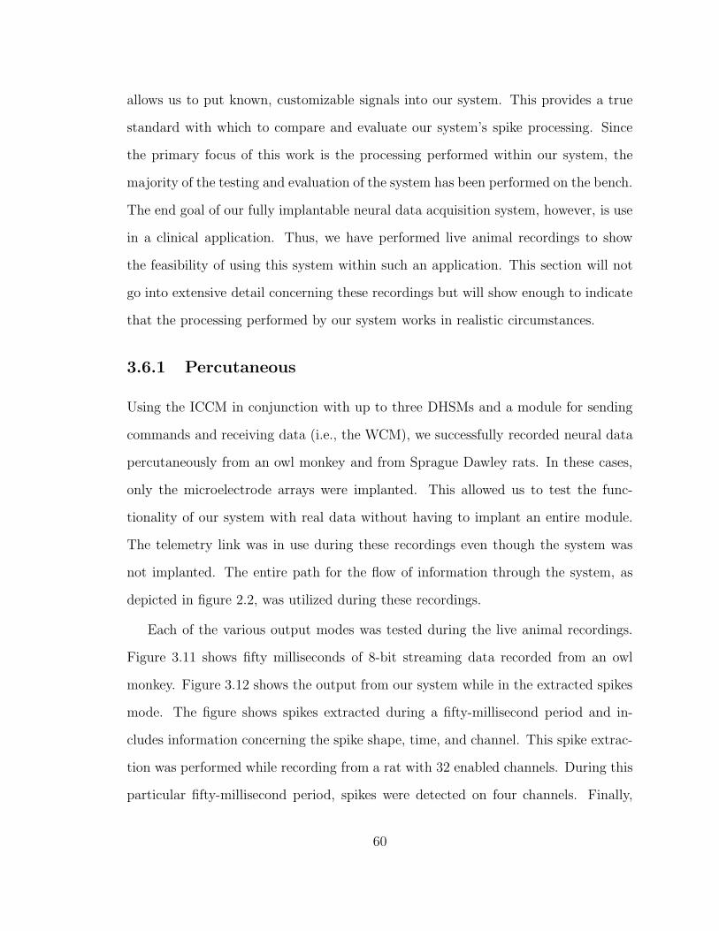
allows us to put known, customizable signals into our system. This provides a true
standard with which to compare and evaluate our system’s spike processing. Since
the primary focus of this work is the processing performed within our system, the
majority of the testing and evaluation of the system has been performed on the bench.
The end goal of our fully implantable neural data acquisition system, however, is use
in a clinical application. Thus, we have performed live animal recordings to show
the feasibility of using this system within such an application. This section will not
go into extensive detail concerning these recordings but will show enough to indicate
that the processing performed by our system works in realistic circumstances.
3.6.1 Percutaneous
Using the ICCM in conjunction with up to three DHSMs and a module for sending
commands and receiving data (i.e., the WCM), we successfully recorded neural data
percutaneously from an owl monkey and from Sprague Dawley rats. In these cases,
only the microelectrode arrays were implanted. This allowed us to test the func-
tionality of our system with real data without having to implant an entire module.
The telemetry link was in use during these recordings even though the system was
not implanted. The entire path for the flow of information through the system, as
depicted in figure 2.2, was utilized during these recordings.
Each of the various output modes was tested during the live animal recordings.
Figure 3.11 shows fifty milliseconds of 8-bit streaming data recorded from an owl
monkey. Figure 3.12 shows the output from our system while in the extracted spikes
mode. The figure shows spikes extracted during a fifty-millisecond period and in-
cludes information concerning the spike shape, time, and channel. This spike extrac-
tion was performed while recording from a rat with 32 enabled channels. During this
particular fifty-millisecond period, spikes were detected on four channels. Finally,
60

5 ms
100 µV
Figure 3.11: Output of the streaming data mode. The figure shows fifty millisecondsof data recorded from an owl monkey.
figure 3.13 shows the output of the streaming data with extracted spikes mode. This
includes fifty milliseconds of raw neural data followed by the spike extracted during
that time period.
The fact that these recordings were made percutaneously also allowed us to make
a comparison between data recorded by our system and data recorded by another
commonly used neural data acquisition system. Figure 3.14 shows a comparison
between recordings from a rat. One set of recordings was made using our system and
another set was obtained using a wired Plexon neural data acquisition system. The
two sets of data were recorded sequentially rather than simultaneously. As a result,
the two systems did not record the exact same spikes; however, they did record from
the same neurons. Channel 17 in this figure is of particular interest since two clearly
distinguishable units are visible. Figure 3.15 shows extracted spikes from channel 17
in two different formats – a typical overlay of the extracted spikes and a density plot,
which aids in visualization of the two distinct units.
Figure 3.16 shows spikes extracted by our system from selected channels over
a roughly one-minute period of recording from an owl monkey. Figure 3.17 shows
61
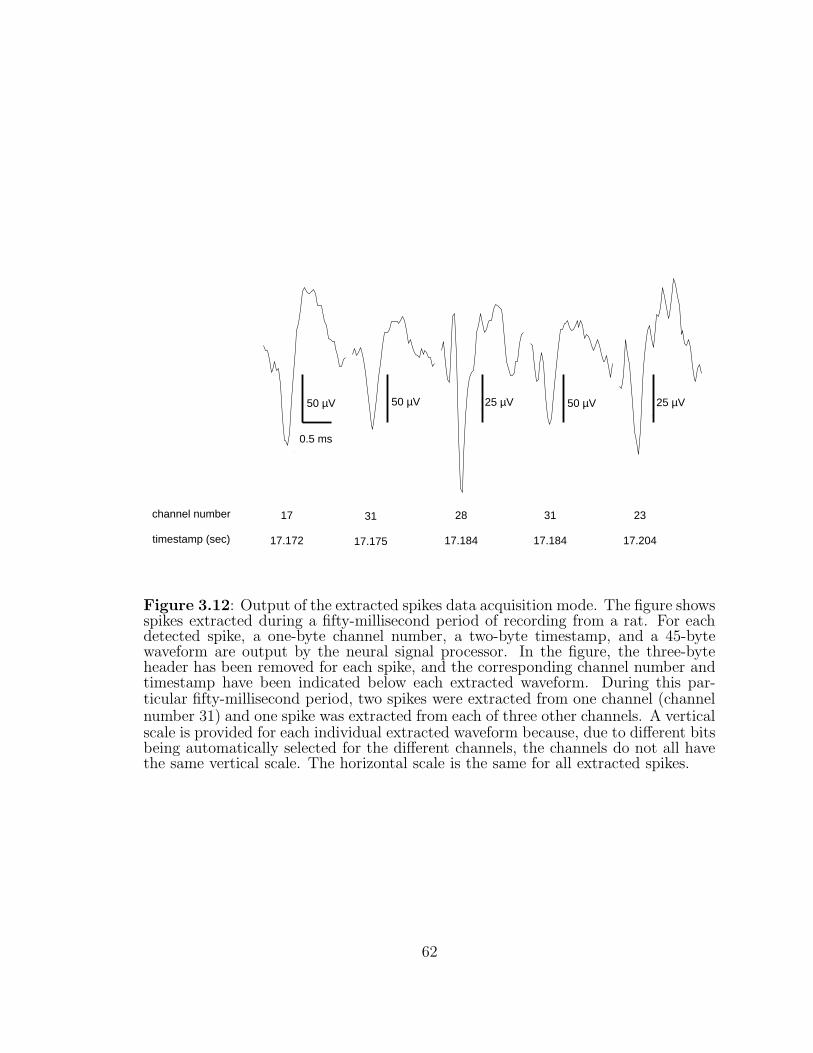
50 µV 50 µV 50 µV25 µV 25 µV
0.5 ms
channel number
timestamp (sec)
17
17.172
31
17.175
28
17.184
31
17.184
23
17.204
Figure 3.12: Output of the extracted spikes data acquisition mode. The figure showsspikes extracted during a fifty-millisecond period of recording from a rat. For eachdetected spike, a one-byte channel number, a two-byte timestamp, and a 45-bytewaveform are output by the neural signal processor. In the figure, the three-byteheader has been removed for each spike, and the corresponding channel number andtimestamp have been indicated below each extracted waveform. During this par-ticular fifty-millisecond period, two spikes were extracted from one channel (channelnumber 31) and one spike was extracted from each of three other channels. A verticalscale is provided for each individual extracted waveform because, due to different bitsbeing automatically selected for the different channels, the channels do not all havethe same vertical scale. The horizontal scale is the same for all extracted spikes.
62
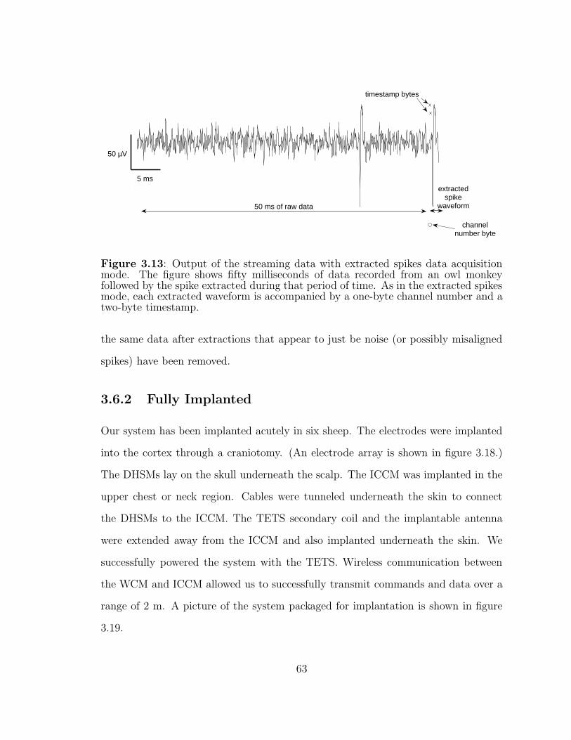
5 ms
50 µV
channelnumber byte
timestamp bytes
50 ms of raw data
extractedspike
waveform
Figure 3.13: Output of the streaming data with extracted spikes data acquisitionmode. The figure shows fifty milliseconds of data recorded from an owl monkeyfollowed by the spike extracted during that period of time. As in the extracted spikesmode, each extracted waveform is accompanied by a one-byte channel number and atwo-byte timestamp.
the same data after extractions that appear to just be noise (or possibly misaligned
spikes) have been removed.
3.6.2 Fully Implanted
Our system has been implanted acutely in six sheep. The electrodes were implanted
into the cortex through a craniotomy. (An electrode array is shown in figure 3.18.)
The DHSMs lay on the skull underneath the scalp. The ICCM was implanted in the
upper chest or neck region. Cables were tunneled underneath the skin to connect
the DHSMs to the ICCM. The TETS secondary coil and the implantable antenna
were extended away from the ICCM and also implanted underneath the skin. We
successfully powered the system with the TETS. Wireless communication between
the WCM and ICCM allowed us to successfully transmit commands and data over a
range of 2 m. A picture of the system packaged for implantation is shown in figure
3.19.
63
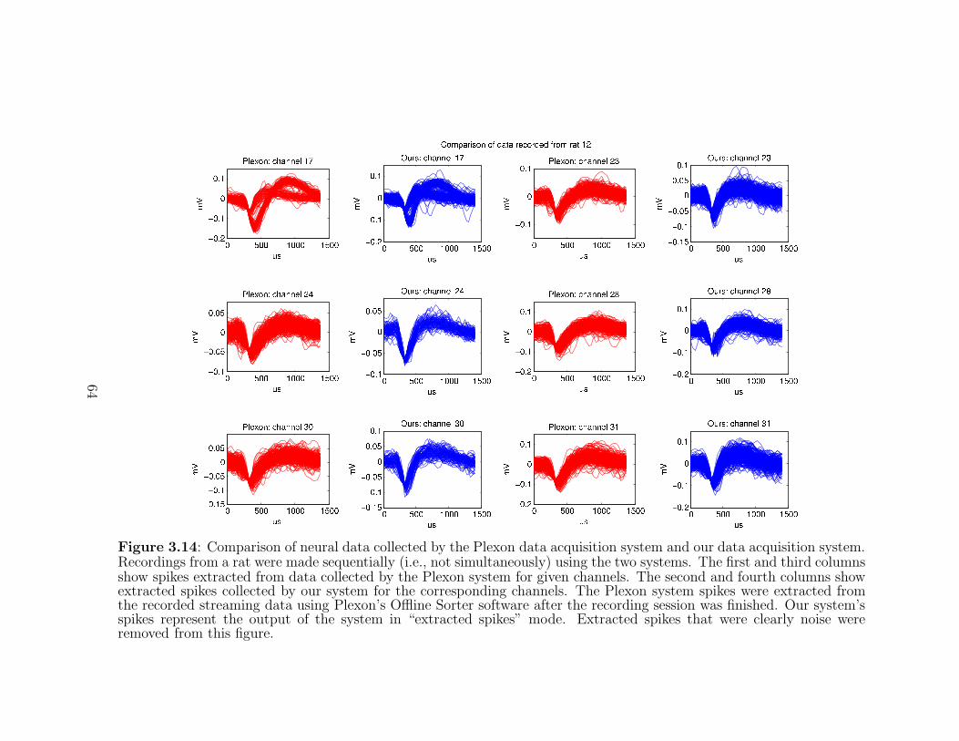
Figure 3.14: Comparison of neural data collected by the Plexon data acquisition system and our data acquisition system.Recordings from a rat were made sequentially (i.e., not simultaneously) using the two systems. The first and third columnsshow spikes extracted from data collected by the Plexon system for given channels. The second and fourth columns showextracted spikes collected by our system for the corresponding channels. The Plexon system spikes were extracted fromthe recorded streaming data using Plexon’s Offline Sorter software after the recording session was finished. Our system’sspikes represent the output of the system in “extracted spikes” mode. Extracted spikes that were clearly noise wereremoved from this figure.
64
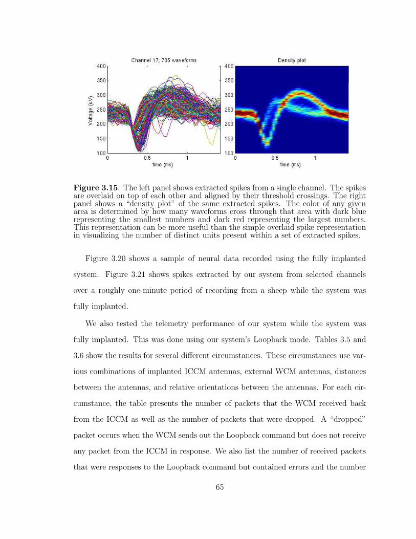
Figure 3.15: The left panel shows extracted spikes from a single channel. The spikesare overlaid on top of each other and aligned by their threshold crossings. The rightpanel shows a “density plot” of the same extracted spikes. The color of any givenarea is determined by how many waveforms cross through that area with dark bluerepresenting the smallest numbers and dark red representing the largest numbers.This representation can be more useful than the simple overlaid spike representationin visualizing the number of distinct units present within a set of extracted spikes.
Figure 3.20 shows a sample of neural data recorded using the fully implanted
system. Figure 3.21 shows spikes extracted by our system from selected channels
over a roughly one-minute period of recording from a sheep while the system was
fully implanted.
We also tested the telemetry performance of our system while the system was
fully implanted. This was done using our system’s Loopback mode. Tables 3.5 and
3.6 show the results for several different circumstances. These circumstances use var-
ious combinations of implanted ICCM antennas, external WCM antennas, distances
between the antennas, and relative orientations between the antennas. For each cir-
cumstance, the table presents the number of packets that the WCM received back
from the ICCM as well as the number of packets that were dropped. A “dropped”
packet occurs when the WCM sends out the Loopback command but does not receive
any packet from the ICCM in response. We also list the number of received packets
that were responses to the Loopback command but contained errors and the number
65
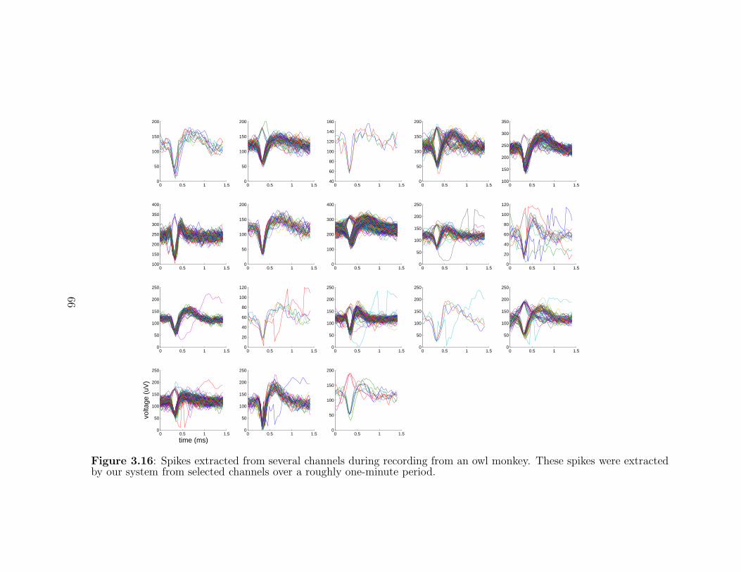
0 0.5 1 1.50
50
100
150
200
0 0.5 1 1.50
50
100
150
200
0 0.5 1 1.540
60
80
100
120
140
160
0 0.5 1 1.50
50
100
150
200
0 0.5 1 1.5100
150
200
250
300
350
0 0.5 1 1.5100
150
200
250
300
350
400
0 0.5 1 1.50
50
100
150
200
0 0.5 1 1.50
100
200
300
400
0 0.5 1 1.50
50
100
150
200
250
0 0.5 1 1.50
20
40
60
80
100
120
0 0.5 1 1.50
50
100
150
200
250
0 0.5 1 1.50
20
40
60
80
100
120
0 0.5 1 1.50
50
100
150
200
250
0 0.5 1 1.50
50
100
150
200
250
0 0.5 1 1.50
50
100
150
200
250
0 0.5 1 1.50
50
100
150
200
250
time (ms)
volta
ge (
uV)
0 0.5 1 1.50
50
100
150
200
250
0 0.5 1 1.50
50
100
150
200
Figure 3.16: Spikes extracted from several channels during recording from an owl monkey. These spikes were extractedby our system from selected channels over a roughly one-minute period.
66
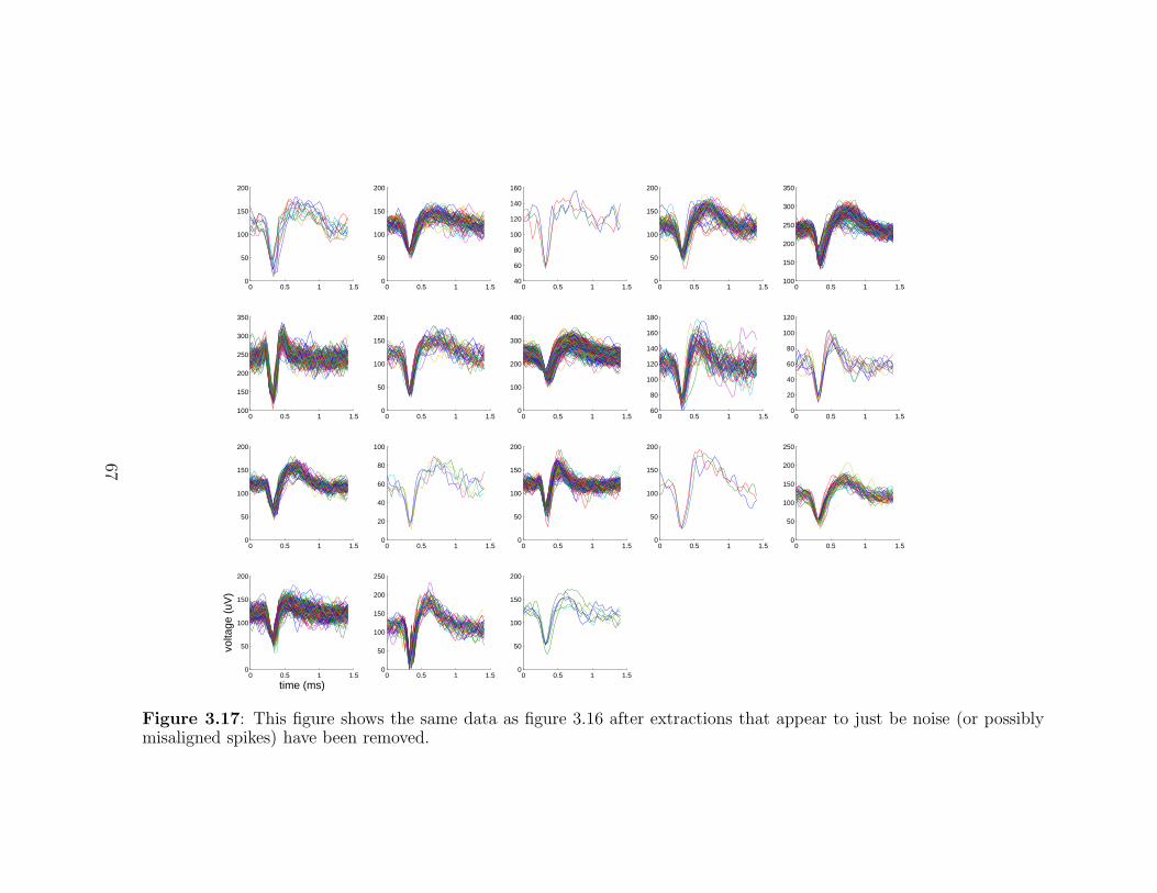
0 0.5 1 1.50
50
100
150
200
0 0.5 1 1.50
50
100
150
200
0 0.5 1 1.540
60
80
100
120
140
160
0 0.5 1 1.50
50
100
150
200
0 0.5 1 1.5100
150
200
250
300
350
0 0.5 1 1.5100
150
200
250
300
350
0 0.5 1 1.50
50
100
150
200
0 0.5 1 1.50
100
200
300
400
0 0.5 1 1.560
80
100
120
140
160
180
0 0.5 1 1.50
20
40
60
80
100
120
0 0.5 1 1.50
50
100
150
200
0 0.5 1 1.50
20
40
60
80
100
0 0.5 1 1.50
50
100
150
200
0 0.5 1 1.50
50
100
150
200
0 0.5 1 1.50
50
100
150
200
250
0 0.5 1 1.50
50
100
150
200
time (ms)
volta
ge (
uV)
0 0.5 1 1.50
50
100
150
200
250
0 0.5 1 1.50
50
100
150
200
Figure 3.17: This figure shows the same data as figure 3.16 after extractions that appear to just be noise (or possiblymisaligned spikes) have been removed.
67

Figure 3.18: Microwire electrode array. This array contains tungsten electrodes for32 channels. It also has two reference electrodes. Arrays like this one were connectedto DHSMs and implanted during the acute sheep studies.
of packets that were received but were responses to incorrect commands (i.e., the
ICCM misinterpreted the command from the WCM as something other than a Loop-
back command). These results are not meant to be a comprehensive evaluation of
the telemetry performance of the implanted system. Rather, they give a general idea
of the level of performance under different circumstances. It should be noted that
we adjusted the antenna matching network after sheep #4. This improved tuning
resulted in better telemetry performance for sheep #5 and #6.
68
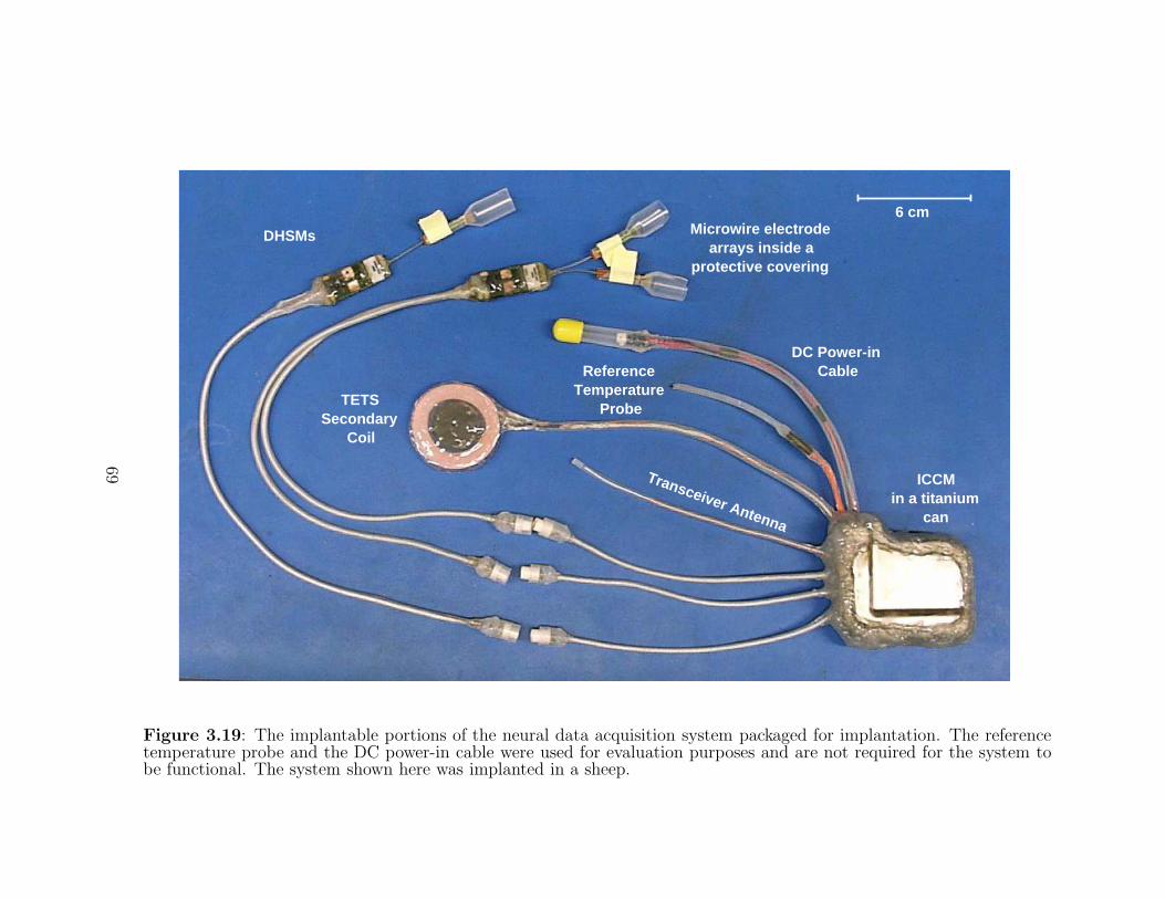
DC Power-in Cable
TETS Secondary
Coil
DHSMs
Transceiver Antenna
Reference Temperature
Probe
ICCM in a titanium
can
6 cm Microwire electrode
arrays inside a protective covering
Figure 3.19: The implantable portions of the neural data acquisition system packaged for implantation. The referencetemperature probe and the DC power-in cable were used for evaluation purposes and are not required for the system tobe functional. The system shown here was implanted in a sheep.
69

0 1000 2000 3000 4000 5000 600060
80
100
120
140
160
180
time (ms)
Vol
tage
(uV
)
(a)
2130 2135 2140 2145 2150 2155 2160 2165 2170
50
100
150
200
time (ms)
Vol
tage
(uV
)
(b)
Figure 3.20: (a) Streaming neural data recorded by our system while it was fullyimplanted in a sheep. (b) A zoomed in portion of some of the data. The threesolid arrows point to spikes that presumably came from a neuron near this particularchannel’s electrode. The dashed arrow points to a spike that presumably came froma neuron near the reference electrode. See section 4.8 for more on this.
70
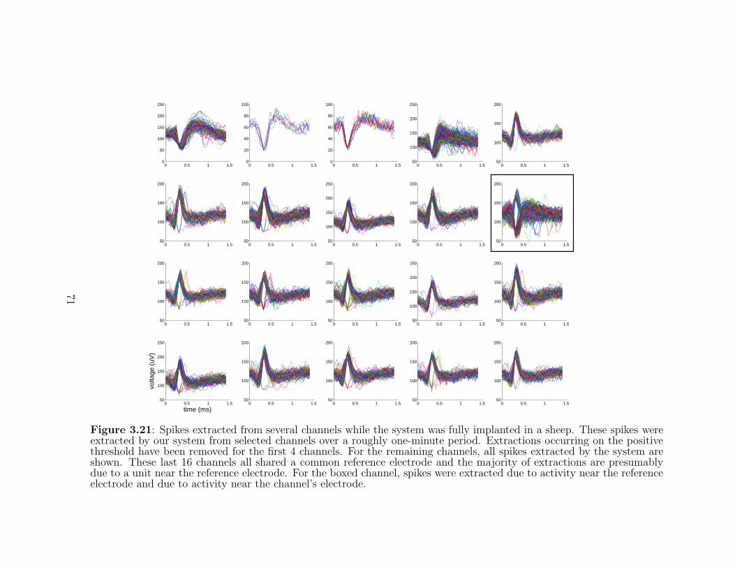
0 0.5 1 1.50
50
100
150
200
250
0 0.5 1 1.50
20
40
60
80
100
0 0.5 1 1.50
20
40
60
80
100
0 0.5 1 1.550
100
150
200
0 0.5 1 1.550
100
150
200
0 0.5 1 1.550
100
150
200
0 0.5 1 1.550
100
150
200
250
0 0.5 1 1.550
100
150
200
0 0.5 1 1.550
100
150
200
0 0.5 1 1.550
100
150
200
0 0.5 1 1.550
100
150
200
0 0.5 1 1.550
100
150
200
0 0.5 1 1.550
100
150
200
250
0 0.5 1 1.550
100
150
200
0 0.5 1 1.550
100
150
200
250
time (ms)
volta
ge (
uV)
0 0.5 1 1.550
100
150
200
0 0.5 1 1.550
100
150
200
0 0.5 1 1.550
100
150
200
0 0.5 1 1.550
100
150
200
0 0.5 1 1.550
100
150
200
250
Figure 3.21: Spikes extracted from several channels while the system was fully implanted in a sheep. These spikes wereextracted by our system from selected channels over a roughly one-minute period. Extractions occurring on the positivethreshold have been removed for the first 4 channels. For the remaining channels, all spikes extracted by the system areshown. These last 16 channels all shared a common reference electrode and the majority of extractions are presumablydue to a unit near the reference electrode. For the boxed channel, spikes were extracted due to activity near the referenceelectrode and due to activity near the channel’s electrode.
71
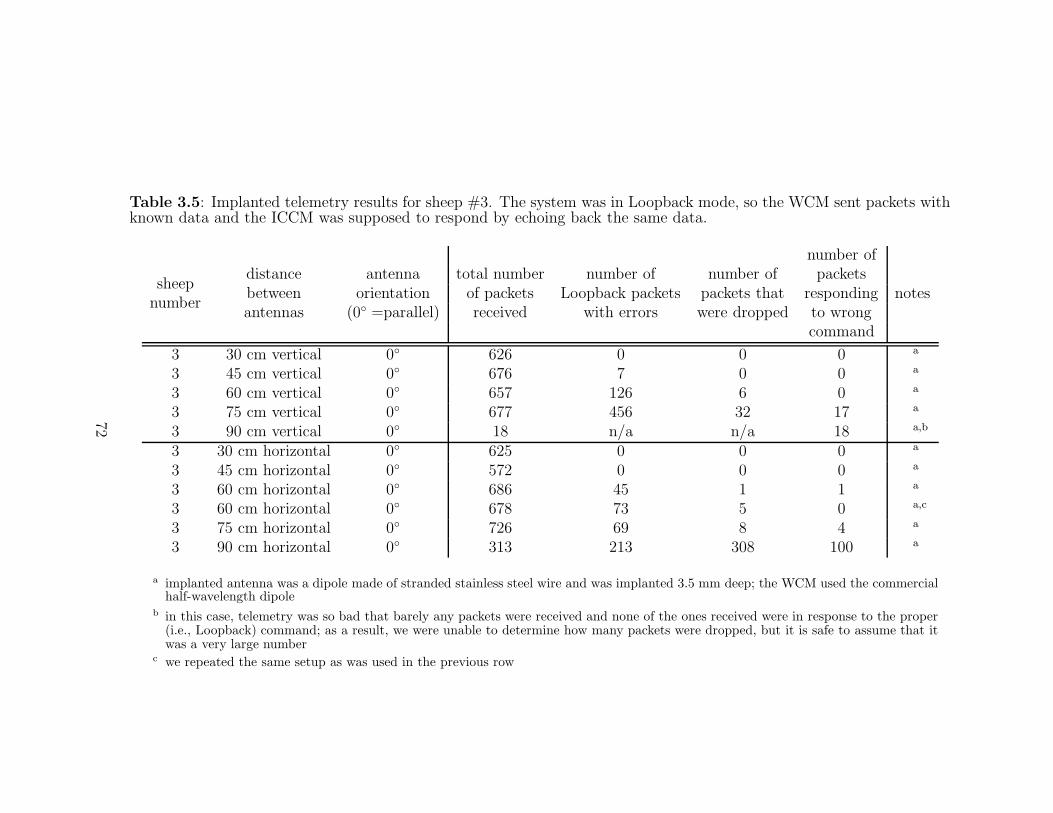
Table 3.5: Implanted telemetry results for sheep #3. The system was in Loopback mode, so the WCM sent packets withknown data and the ICCM was supposed to respond by echoing back the same data.
number of
sheepdistance antenna total number number of number of packets
numberbetween orientation of packets Loopback packets packets that responding notesantennas (0◦ =parallel) received with errors were dropped to wrong
command
3 30 cm vertical 0◦ 626 0 0 0 a
3 45 cm vertical 0◦ 676 7 0 0 a
3 60 cm vertical 0◦ 657 126 6 0 a
3 75 cm vertical 0◦ 677 456 32 17 a
3 90 cm vertical 0◦ 18 n/a n/a 18 a,b
3 30 cm horizontal 0◦ 625 0 0 0 a
3 45 cm horizontal 0◦ 572 0 0 0 a
3 60 cm horizontal 0◦ 686 45 1 1 a
3 60 cm horizontal 0◦ 678 73 5 0 a,c
3 75 cm horizontal 0◦ 726 69 8 4 a
3 90 cm horizontal 0◦ 313 213 308 100 a
a implanted antenna was a dipole made of stranded stainless steel wire and was implanted 3.5 mm deep; the WCM used the commercialhalf-wavelength dipole
b in this case, telemetry was so bad that barely any packets were received and none of the ones received were in response to the proper(i.e., Loopback) command; as a result, we were unable to determine how many packets were dropped, but it is safe to assume that itwas a very large number
c we repeated the same setup as was used in the previous row
72
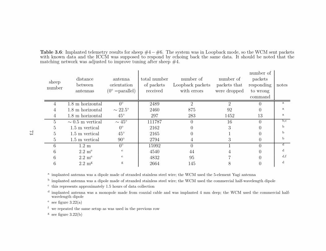
Table 3.6: Implanted telemetry results for sheep #4−#6. The system was in Loopback mode, so the WCM sent packetswith known data and the ICCM was supposed to respond by echoing back the same data. It should be noted that thematching network was adjusted to improve tuning after sheep #4.
number of
sheepdistance antenna total number number of number of packets
numberbetween orientation of packets Loopback packets packets that responding notesantennas (0◦ =parallel) received with errors were dropped to wrong
command
4 1.8 m horizontal 0◦ 2489 2 2 0 a
4 1.8 m horizontal ∼ 22.5◦ 2460 875 92 0 a
4 1.8 m horizontal 45◦ 297 283 1452 13 a
5 ∼ 0.5 m vertical ∼ 45◦ 111787 0 16 0 b,c
5 1.5 m vertical 0◦ 2162 0 3 0 b
5 1.5 m vertical 45◦ 2165 0 1 0 b
5 1.5 m vertical 90◦ 2794 4 3 0 b
6 1.2 m 0◦ 15992 0 1 0 d
6 2.2 me e 4540 44 4 0 d
6 2.2 me e 4832 95 7 0 d,f
6 2.2 mg g 2664 145 8 0 d
a implanted antenna was a dipole made of stranded stainless steel wire; the WCM used the 5-element Yagi antennab implanted antenna was a dipole made of stranded stainless steel wire; the WCM used the commercial half-wavelength dipolec this represents approximately 1.5 hours of data collectiond implanted antenna was a monopole made from coaxial cable and was implanted 4 mm deep; the WCM used the commercial half-
wavelength dipolee see figure 3.22(a)f we repeated the same setup as was used in the previous rowg see figure 3.22(b)
73
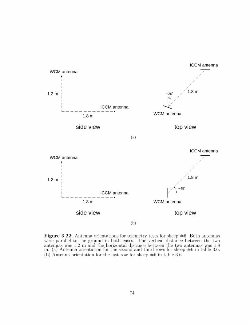
WCM antenna
ICCM antenna
side view top view
1.2 m
1.8 m
1.8 m
ICCM antenna
WCM antenna
~20˚
(a)
WCM antenna
ICCM antenna
side view top view
1.2 m
1.8 m
1.8 m
ICCM antenna
WCM antenna
~45˚
(b)
Figure 3.22: Antenna orientations for telemetry tests for sheep #6. Both antennaswere parallel to the ground in both cases. The vertical distance between the twoantennas was 1.2 m and the horizontal distance between the two antennas was 1.8m. (a) Antenna orientation for the second and third rows for sheep #6 in table 3.6.(b) Antenna orientation for the last row for sheep #6 in table 3.6.
74
Chapter 4
System Discussion
4.1 Spike Detection
In section 3.2.3, we presented the spike detection results for various SNRs and thresh-
old multipliers. We compared spike detection as performed by our system with offline
spike detection performed on the waveform seen by the neural signal processor and
with offline spike detection performed on the original input waveform. These results,
in terms of the probability of detection and rate of false alarms metrics, were pre-
sented in figure 3.4. The similarity between the spike detection performance of our
system and the performance of offline spike detection on the waveform seen by the
neural signal processor confirms that our system is detecting spikes in the intended
manner.
A few further comments about the results are necessary. The probability of de-
tection versus multiplier value curve for the offline spike detection performed on the
original input waveform shifts to the right relative to the curves for the other two
circumstances as the SNR increases. This is due to the fact, as mentioned earlier,
that the act of passing the signal through the neural signal simulator and the DHSMs
adds some noise and performs some filtering on the signal. The end result is that the
SNR of the signal seen by the neural signal processor is lower than that of the signal
used as input to the neural signal simulator. This can be seen by comparing figures
3.3(a) and 3.3(b).
The performance of the system’s spike detection and that of the offline detection
performed on the waveform seen by the neural signal processor match fairly well.
They, however, are not identical even though the same waveform is used in both cir-
75
cumstances. Again, as mentioned earlier, this is due to the fact that the thresholds
used in the two cases were not identical. The threshold used by the neural signal
processor was based on a randomly selected 4096-sample window for each waveform
while the threshold used during offline detection was based on the entire 2-second
waveform. This difference in how thresholds were computed also explains the in-
creased variability in spike detection performance across alpha values for our system
relative to the other two circumstances.
A final difference among the spike detection performance of the three cases is that
at low alpha values our system consistently resulted in a lower rate of false alarms
and oftentimes in a lower probability of detection when compared to the two offline
detection cases. This is due to the buffering within the neural signal processor. As
mentioned in section 2.2.1, when acquiring data in the streaming data with extracted
spikes mode (the mode used to evaluate our system’s spike detection performance),
two-kilobyte FIFOs are used to store extracted spikes until they are ready to be
transmitted. At very low alpha values, the spike detection threshold is very low and
many extractions take place during each 50-ms period. The two-kilobyte FIFO can
hold a maximum of 42 extracted spikes. Once the FIFO has 42 spikes in it, no more
spikes can be stored in it until spikes are transmitted out of the FIFO. Consequently,
it is possible that some detected spikes will never make it into the FIFO, never be
transmitted, and ultimately not show up as detected spikes when computing our
system’s spike detection performance. Since at very low thresholds most detections
do not represent true spikes, the end result is primarily a decrease in the rate of false
alarms. An example of the overflow of the FIFO can be seen in figure 4.1. In this
figure we see that 36 spikes were extracted in a particular 50-ms period. All of these
fit easily into the FIFO. At the end of this 50-ms period, the streaming data for that
period (the “previous” period in the figure) is sent from the ICCM before the spikes
76

from that period are read out of the FIFO and transmitted. Since it takes roughly
15 ms to transmit the streaming data, the 36 spikes remain in the FIFO for the first
15 ms of the next period. In the figure we see that six more spikes are extracted
before there is a significant jump in the timestamp of extracted spikes. Once these
six spikes have been extracted, the FIFO holds a total of 42 spikes and is full. After
the spikes from the previous 50-ms period begin to be transmitted, the FIFO has
available space and newly extracted spikes are once again stored in it. In this figure,
we see that the one true spike was not extracted because it happened to occur during
the period of time in which the FIFO was full. The difference between our system’s
spike detection performance and that of an offline analysis of the waveform presents
no significant concern since it only occurs at very low alpha values. At these low
alpha values, thresholds are so low that almost all extractions are false detections,
so reasonable spike detection performance is not present regardless of whether some
extractions are missed. The difference in performance due to buffering vanishes at
thresholds that are near or above the noise floor. These are the thresholds that are
actually useful and practical for our system.
4.2 Data Reduction due to Spike Extraction
The amount of data reduction resulting from spike extraction ultimately depends on
the rate at which spikes are being detected. The total number of spikes that are
present in the recorded waveforms depends on two factors – the number of neurons
from which the electrodes are recording and the firing rates of these neurons. The
system described here has 96 channels. It is very unlikely that active units will be
present on all 96 channels. However, having 60% to 80% of the channels yield active
units is not unreasonable [17, 52]. Having a single electrode record from multiple
neurons is also quite common. As a result, a value of 1 to 2 is realistic for the ratio
77
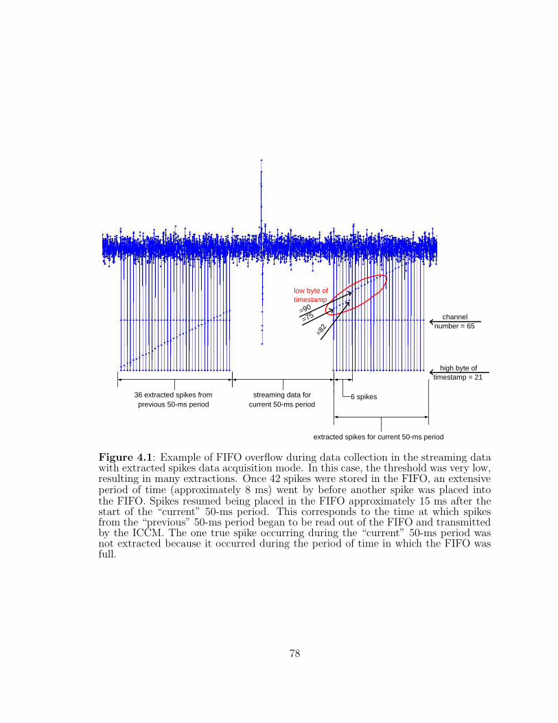
36 extracted spikes from previous 50-ms period
streaming data for current 50-ms period
extracted spikes for current 50-ms period
6 spikes
high byte of timestamp = 21
channel number = 65
low byte of timestamp
=75 =8
2
=90
Figure 4.1: Example of FIFO overflow during data collection in the streaming datawith extracted spikes data acquisition mode. In this case, the threshold was very low,resulting in many extractions. Once 42 spikes were stored in the FIFO, an extensiveperiod of time (approximately 8 ms) went by before another spike was placed intothe FIFO. Spikes resumed being placed in the FIFO approximately 15 ms after thestart of the “current” 50-ms period. This corresponds to the time at which spikesfrom the “previous” 50-ms period began to be read out of the FIFO and transmittedby the ICCM. The one true spike occurring during the “current” 50-ms period wasnot extracted because it occurred during the period of time in which the FIFO wasfull.
78
of total units to electrodes [17, 52]. Thus, a generous estimate of the total number
of neurons from which the electrodes of a 96-channel system might record is 200.
Typical neural firing rates fall in the range of roughly 1 to 10 spikes per second for
resting neurons and roughly 10 to 100 spikes for active neurons [53]. At any given
time, only a fraction of the neurons will be active. Assuming an average firing rate
of 20 spikes per second per neuron, the extracted spikes mode would need to output
192 kilobytes per second (kBps).
(200 neurons)
(
20 spikes/s
neuron
) (
48 bytes
spike
)
= 192 kBps
In order to output all samples for all channels at 8 bits each, an output data rate of
3000 kBps would be needed.
(
31.25 kBps
channel
)
(96 channels) = 3000 kBps
Consequently, spike extraction can be expected to reduce the amount of data by
roughly a factor of 15. A spike extraction scheme similar to the one described here
has been used in live neural recordings and was found to reduce data by 97% [43].
Data reduction through spike extraction is only beneficial if spikes are detected
properly. If true spikes are not detected, valuable information will be lost. If detec-
tions are made where no true spikes are present, the efficiency of the data reduction
will decrease. As stated in section 2.2.1, our system performs spike detection by
applying a threshold to the absolute value of the data. This is a computationally
simple method of performing spike detection. While more complex spike detection
algorithms exist and may provide better performance, this thresholding method is
suitable for a system with limited computational resources [48]. (A detailed evalua-
tion of spike detection methods will not be presented here. See [48,54–61] as well as
chapter 6 for more on spike detection.)
79
4.3 Spike Extraction Limitations
In an ideal neural data acquisition system, the performance of spike extraction would
be equivalent to that of spike detection. For each detection, a given number of samples
before and after the detection point would be stored as the extracted spike waveform.
As long as spikes were detected successfully, there would be no reason for them to not
be extracted properly. However, in systems with limited resources, such as the one
described here, spike detection is only one factor in determining how well extracted
spikes can be acquired by the system. In a fully implantable neural data acquisition
system, memory and data rate limitations must be considered as well. A spike that
has been extracted must be stored in memory until it can be transferred out of the
body via the telemetry link. In our system, the telemetry link has a finite data rate
that allows for a maximum of one hundred extracted spikes to be transmitted in a
given fifty-millisecond period. Consequently, if too many spikes are extracted within
a given period of time, the ICCM will be unable to store and transmit some of them.
These spikes must simply be dropped from the output datastream.
The results presented in section 3.2.4 indicate that the major factor in determin-
ing when spikes will be dropped is the total spike rate across all channels. For all
three distributions of enabled channels, the first FIFO overflows were observed when
the total spike rate was slightly more than 2000 spikes per second. A rate of 2000
spikes per second corresponds to a rate of 100 spikes per fifty-millisecond period.
Considering that the neural signal processor can output a maximum of 100 spikes
per fifty-millisecond period, it is not surprising that spikes are dropped once this rate
is exceeded. If more than 100 spikes are detected in a fifty-millisecond period, the
transmit buffer will be full and spikes will begin to accumulate in the individual data
reduction module FIFOs. If spike rates remain above the 100 spikes per fifty mil-
lisecond limit for an extended period of time, the FIFOs will eventually fill up and be
80

unable to hold more spikes. In the two cases in which 16 channels were enabled and
the firing rate per channel was 125 spikes per second, no overflow of the FIFOs oc-
curred. These cases correspond to having exactly 100 spikes in each fifty-millisecond
period. As expected, no spikes are dropped as long as the spike limit is not surpassed.
The test setup used in section 3.2.4 allowed us to essentially look at FIFO overflow
as a function of firing rate. It must be noted, however, that realistic neural data is very
unlikely to have perfectly constant firing rates. The results that we have presented
represent “steady-state” behaviors. In other words, the results show how our system
behaves after the firing rates of the inputs have been constant for a significant period
of time (on the order of one second). In cases in which the overall firing rate is greater
than 100 spikes per fifty milliseconds, the steady-state behavior occurs only after the
FIFOs have had enough time to gradually fill up. In fact, the FIFOs can serve as
temporary buffers so that the system can accommodate brief periods of overall spike
rates in excess of the 100 spikes per fifty milliseconds limit without dropping any
spikes.
The results presented in section 3.2.4 indicate that the steady-state behaviors of
the two channel distributions with 16 enabled channels are very similar. However,
these two cases differ in how long they take to reach this steady state. In the case
in which the 16 channels were split between two different data reduction modules,
approximately twice as many packets were sent before an occurrence of FIFO overflow
as in the case in which the 16 channels all belonged to the same data reduction
module. This difference in “transient” behavior is a result of the fact that during the
pre-steady-state period, the individual FIFOs in the former case are in essence each
filling up at half the rate of the single FIFO in the latter case.
The steady-state behavior of the neural signal processor is mostly determined by
the total spike rate across all channels while the transient behavior is additionally
81
influenced by the distribution of enabled channels. As a result, the circumstances
under which spikes will be dropped are largely determined by the overall distribution
of spikes in time with some influence by the distribution of spikes in space.
As mentioned in section 3.2.2, no noise was incorporated into any of the waveforms
used for these experiments. This was done intentionally so that only “true” spikes
would be detected and extracted. By eliminating false detections, we were able to
carefully control how many spikes were extracted over a given period of time. With
real neural data, however, it must be assumed that some false detections will occur.
Noise that is incorrectly extracted as a spike will take up space in the transmit buffer
and could contribute to overflows of the FIFOs.
4.4 Latency
Even when spikes are not dropped, high spike rates may increase the delay between
when the spikes are detected and when they are transmitted [62]. The ICCM trans-
mits extracted spikes once every fifty milliseconds. If the telemetry system had
infinite bandwidth, then the expected average latency would be 25 milliseconds and
we would expect the latencies to be uniformly distributed between 0 and 50 millisec-
onds. Spikes that occur near the beginning of a fifty-millisecond period would be
expected to have a latency close to 50 ms while spikes that occur near the end of
a fifty-millisecond period would be expected to have a latency close to 0 ms. How-
ever, since the implantable module can only transmit a finite amount of data during
each fifty-millisecond period, it is possible that spikes which are detected during one
fifty-millisecond period will not be able to be transmitted at the end of that fifty-
millisecond period, thus increasing the average latency. Also, the amount of time
required to transmit a complete packet increases as the size of the packet increases.
As a result, packets that contain large numbers of spikes will take a non-negligible
82

amount of time to be transmitted. Spikes in such packets will also have a higher
than ideal average latency. For a clinical BMI, total latencies should be less than 200
milliseconds [63].
Our results show that latencies do vary with total firing rate. However, even in
the worst case that we tested, the latencies remained safely below 200 ms. In the
first trial, very few spikes were present. The distribution of latencies as presented in
figure 3.6(a) is close to what would be expected in the ideal case described above.
The mean latency, 26.7 ms, and the distribution of latencies indicate that no more
than roughly 2 ms of latency are added by processing in the system. Almost all
latency present in this case is due to the fact that extracted spikes are transmitted
by the ICCM at the end of fifty-millisecond periods.
In the second trial, the overall firing rate was approximately 1000 spikes per
second, or 50 spikes per 50 ms. This is one half of the 100 spikes per fifty-millisecond
period limit. Figure 3.6(b) again shows a relatively uniform distribution of latencies
over a fifty-millisecond range. However, the mean and distribution are shifted up by
approximately 25 ms from the first case. This is a result of the fact that the WCM
waits until it has received an entire packet before it is ready to perform further
processing on any of the extracted spikes. The 25 ms shift is due directly to the fact
that a packet containing 50 spikes takes approximately 25 ms to be transmitted.
In the third trial, the overall firing rate was just under 2000 spikes per second,
or 100 spikes per 50 ms. Even though no spikes were dropped during this trial,
each packet was either full or nearly full. Once again, figure 3.6(c) shows a more
or less uniform distribution of latencies over a fifty-millisecond range. The mean
and distribution are shifted up by approximately 50 ms from the first case and by
approximately 25 ms from the second case. Again, this shift is due to the fact that
a packet containing 100 spikes takes approximately 50 ms to be transmitted.
83

In the final trial, the overall firing rate was approximately 2125 spikes per second.
This rate exceeded the 100 spikes per fifty-millisecond limit and resulted in dropped
spikes. Spikes that were not dropped had latencies that were relatively uniformly
distributed between about 95 ms and 145 ms. The large increase in latencies as
compared to the previous case can be explained by the fact that in most cases during
this trial, spikes that were detected during one fifty-millisecond period would be
unable to be transmitted at the end of that period. Rather, they would be forced to
sit in the neural signal processor until the end of the next fifty-millisecond period.
Figure 3.6(d) has two significant features – the presence of dropped spikes and
the noticeable dip in the 100 ms to 105 ms range. These two features are most likely
related. Since the overall firing rate in this case is not tremendously greater than
the 100 spikes per 50 ms limit, the buffers would only be completely filled near the
end of a given fifty-millisecond period. Consequently, spikes would only be dropped
if they occurred near the end of a fifty-millisecond period. If these spikes had not
been dropped, they would be expected to have a latency of approximately 100 ms –
50 ms due to sitting in the neural signal processor for an extra period as a result of a
full transmit buffer followed by another 50 ms required for transmitting a full packet.
Thus, the dip in the histogram is a result of the fact that spikes that would have
fallen within a specific latency range were dropped instead of being transmitted.
We do not foresee problems with the latencies measured here. However, if nec-
essary, it is possible to decrease the latency. The total latency within our system is
essentially made up of the following two components: 1) the time from when a spike
is detected until it is transmitted and 2) the time from when a spike is received by the
external module until it is ready for further use within that module. The latency con-
tributed by the first component is basically the time between when a spike is detected
and when a given 50-ms period ends. Since the timing of spikes is independent of the
84
times at which 50-ms periods start and end, we would expect this first component
to contribute on average 25 ms of latency. Reducing the interval between when the
WCM sends commands (and consequently between when the neural signal processor
responds to commands) would in turn reduce the first component of latency. For
example, if spikes were sent out of the ICCM every 20 ms instead of every 50 ms,
on average the time between when a spike would be detected and when it would be
transmitted would be roughly 10 ms. The trade-off for increasing the frequency at
which packets are sent out of the ICCM is that a larger percentage of the available
bandwidth will need to be used for transmitting packet overhead. This is a result of
the fact that each packet has a fixed amount of overhead and more packets will be
transmitted when commands are received at a higher frequency.
The latency contributed by the second component is a direct result of the way
the WCM processes data. Currently our WCM does not use any of the data that
it has received until it has received a complete packet. This is done so that error
checking (through the use of a parity byte) can be performed before any of the data
are processed further. Since a full packet can take up to almost 50 ms to transmit, the
possibility exists that data will sit in the WCM for a significant amount of time before
it is used. An alternative, which would essentially eliminate this component of the
latency, is to allow the WCM to use data as soon as it is received. The consequence
in this case is that simple error-checking schemes that depend on knowledge of the
contents of an entire packet will have extremely limited usefulness.
4.5 Flexibility
While we anticipate that our system will primarily be used in the extracted spikes
mode, we have implemented it in such a way that flexibility in how data reduc-
tion is performed is available. Many different research and clinical applications of a
85
neural data acquisition system exist. These applications do not all have the same
requirements regarding the collected neural data. A fully implantable neural data
acquisition system that is flexible enough to perform different forms of data reduction
can be useful in these various applications while still limiting the amount of unnec-
essary information that is sent out and thus reducing the burden on the telemetry
system. Even within a single experiment, flexibility in how data is processed and
output is desirable. For example, while a given experiment might ultimately use the
extracted spikes mode of our system, the streaming data mode could be a valuable
tool for the investigator in making an initial assessment of the quality of the signals
on individual channels. Also, cases exist in which the costs incurred by spike sorting
are not necessarily justified by the potential information gained from this processing
step [64]. In such cases, the flexibility to simply output spike detections, rather than
extracted waveforms, is desirable.
The fact that the processing has been implemented in programmable logic also
provides flexibility. Our design can serve as a starting point for other systems with
signal processing and telemetry needs. The modular nature of the design lends itself
to modifications of individual portions of the system while leaving the overall system
architecture intact.
4.6 Telemetry
Development of the neural signal processor has been centered on the communication
needs of a fully implantable neural data acquisition system. The transceiver interface
clearly plays a crucial role in the telemetry link. Also, the data reduction scheme was
implemented in large part as a response to telemetry limitations. The use of a custom
packet structure and telemetry protocol has allowed us to implement the telemetry
engine along with the data reduction algorithms in a single chip. This has also allowed
86
us to limit overhead so that as much neural data as possible can be efficiently output
by the implanted portion of the system. The command-and-response structure of
our telemetry protocol allows for flexibility in terms of what data can be obtained
from the implantable module. It also allows the external module to determine when
packets are being dropped and the communication pathway is not working properly.
The results of the Loopback test presented in section 3.4 confirm that our system is
capable of successful, reliable bidirectional communication.
It should be noted that our system employs a relatively simple telemetry proto-
col. While the protocol allows for a baseline level of error-checking and allows the
external module to determine when packets are being dropped, it does not provide
a means for the retransmission of dropped commands or data. Since commands are
sent every 50 ms, the WCM can simply repeat a given command (for example, “write
configuration registers” or “read configuration registers”) until it receives a response
from the ICCM. Additionally, the ICCM is set up to send out data at the end of each
50-ms period if the last command that it received was a request for data and it has
not received any commands within the last 50 ms. Given these facts, the dropping
of commands should not pose a significant problem. The more important question is
whether or not providing a means for the retransmission of dropped data is justifiable.
The cost of providing a means of retransmission would be quite high. Implement-
ing a more complex communication protocol would consume valuable computational
resources. More importantly, a significant increase in the amount of space allocated
for storing data would be required since data would need to continue to be stored
in the implantable module even after the original transmission. Otherwise, a future
retransmission of the data would not be possible. The discussion of latency presented
earlier suggests that data that are delayed significantly more than the delays that are
already present in the system will be “too old” to be useful in a real-time system.
87

Providing the capability to retransmit dropped data would likely add significantly to
the latency of the data. Thus, we feel that for a system with limited resources that is
intended to be used in real-time, the benefits of providing a more complex telemetry
protocol do not justify the costs. Clearly, there are limitations to the telemetry sys-
tem presented here. In the context of the full neural data acquisition system, we feel
that these limitations are best addressed through optimization of antennas, antenna
configurations, and device placement rather than through increasing the complexity
of the telemetry protocol.
We presented some data regarding the telemetry performance of the fully im-
planted system in section 3.6.2. We found that telemetry can be performed relatively
successfully over a range of a couple meters. Some implantable systems have a teleme-
try range on the order of a few centimeters rather than on the order of a couple meters.
However, the performance of our system can be sensitive to the relative orientation
between antennas and to the surrounding environment. The operating room in which
the telemetry tests were performed is far from an ideal environment. Additionally, for
a system that is implanted in a living, moving animal or person, the effect of motion
between the implanted portion of the system and the external portion of the system
could prove to have a significant impact on telemetry performance. As stated earlier,
we did not set out to perform a comprehensive evaluation of telemetry performance
for the implanted system. Rather, we have shown that our implanted system can
successfully communicate with an external module over a reasonable range. Teleme-
try is one area in which the environment and circumstances in which the system will
be used should be considered in order to obtain the necessary performance.
88
4.7 Spike Sorting
Our system has been designed to be a component of a BMI. Within a BMI application,
spike sorting is a commonly used signal processing step. The extracted spikes mode
of our system was developed with this in mind. This mode provides the information
necessary for spike sorting to be performed outside of the body where it can be
supervised and modified easily. At the same time, the data that are not necessary
for spike sorting, the baseline voltage trace between spikes, are discarded within the
neural signal processor resulting in significant data reduction. High channel-count
implantable devices that do not provide the extracted spike shape [53,65,66] preclude
standard spike sorting as a further processing step. It should be noted, however, that
some level of spike discrimination might still be possible in such systems. For example,
while the system presented in [65] does not output extracted spike waveforms, it does
provide spike timing and amplitude information, which may be used in discriminating
spikes that are recorded on the same electrode. Nevertheless, to the best of our
knowledge, the neural signal processor presented here is the first implantable, high
channel-count neural signal processor with the capability of outputting extracted
spike waveforms. We have shown that our system can interface well with commercial
spike sorting software. By sending extracted spikes out of the body, our system
allows us to perform spike sorting in a manner similar to that commonly used by
wired, percutaneous recording systems.
Section 2.3.2 stated that the real-time template-matching phase of the spike sort-
ing process is performed in the WCM. An alternative location for performing tem-
plate matching is the ICCM’s neural signal processor. Rather than sending extracted
spikes out of the body and performing template matching in the external processor,
we could extract the spikes and perform the template matching inside the body.
Then, for example, sorted bin counts could be sent out of the body. This would be
89

advantageous because it would significantly decrease the burden on the telemetry
system. We have not implemented template matching in this manner simply because
the ICCM’s FPGA does not have enough resources to perform template matching in
addition to all of its current functions (see section 3.2.1 for more details on the use
of resources within the FPGA). Nevertheless, the potential for performing template
matching within the body exists if the ICCM used an FPGA with more resources
or if we removed some of the functionality of the current neural signal processor.
The implanted neural signal processor is perfectly well-suited to perform template
matching, and due to the modular nature of our processing implementation, the
template-matching module currently located in the WCM’s FPGA could more or
less be dropped into the ICCM’s FPGA as is.
4.8 Live Animal Recordings
As shown in section 3.6, our system successfully recorded and processed neural data
from live animals. A few details regarding these live recordings are worth further
attention. Extracellular action potentials typically have a triphasic shape consisting
of a positive phase followed by a negative phase followed by another positive phase.
The initial positive phase is oftentimes relatively small and may not rise above the
noise floor resulting in what appears to be a biphasic spike. The negative phase
typically has an amplitude at least as large as that of the final positive phase. (Ex-
amples of these general characteristics can be seen in the spikes in figures 3.11-3.17
and 3.20(b).) As a result, when voltage thresholds are used to detect spikes, they are
typically set to detect the negative phase of spikes. Systems that use dual thresholds
(such as ours) typically also end up detecting the negative phase, but crossings of
the positive threshold do occur as well. We have observed that detections due to
a crossing of the positive threshold often fall into one of two categories – (1) noise
90

that crosses the positive threshold or (2) a triphasic spike whose initial positive phase
crossed the positive threshold. In both of these cases, it would often be better if the
positive threshold simply had not been used. In the first case, the noise may not
have crossed the negative threshold; thus, the use of a dual threshold can lead to
more false detections. (Compare figures 3.16 and 3.17 to see this.) In the second
case, since the negative phase of a spike typically has the largest amplitude, the spike
most likely would have still been detected even if the positive threshold had not been
used. Spikes that have an initial positive phase that has an amplitude comparable
to the threshold can lead to alignment issues when spike sorting is performed after
detection using a dual threshold. See the red spikes in figure 3.9 for an example of
alignment issues that can arise due to the use of a dual threshold. (Note that the
spikes in this figure were simulated and are not realistic in shape. Nevertheless, in the
figure, some of the red spikes crossed the threshold during an initial positive phase
while other red spikes did not cross the threshold until the negative phase.) Mis-
alignment can also be seen in some cases in figure 3.16. Our choice to perform spike
detection on the absolute value of the data was based on the results found in [48].
Our limited observations of live animal recordings, however, suggest that there may
be some advantages to simply using a single negative threshold rather than applying
the threshold to the absolute value of the data.
There is a third circumstance in which we have observed crossings of the positive
threshold. Our system performs differential recordings. Each set of 16 channels has a
local reference electrode. If an active neuron is located near the reference electrode,
inverted spikes will appear on each channel that uses that reference electrode. We
observed this in some of our recordings from sheep. Figure 3.20(b) presents an
example of a recording that appears to contain spikes both from a neuron near the
particular channel’s electrode and from a neuron near the reference electrode. The
91
suspicion of the presence of a neuron near the reference electrode was supported in
this case by looking at a logfile recorded while the ICCM was in the extracted spikes
data acquisition mode. In this logfile we found that a significant proportion of the
extracted spikes on the set of 16 channels (see figure 3.21) had identical timestamps
on all 16 channels. It is extremely unlikely that this would have been observed based
on the activity of individual units located near each of the 16 individual electrodes.
4.9 Power Consumption
The power consumption of our neural signal processor is high compared to that of
devices such as those described in [53], [65], and [66]. This is in large part due to
the fact that our device was implemented in an FPGA while the other devices were
implemented in application-specific integrated circuits (ASICs). The exact power
savings gained by implementing a design in an ASIC rather than an FPGA depends
on the specifics of the design, the FPGA, and other factors. Nevertheless, for low-
power systems, a reduction in power consumption by a factor of 10 or more is not
an unreasonable result of switching from an FPGA implementation to an ASIC im-
plementation [67]. Thus, an ASIC implementation of our design would be expected
to consume 10 mW or less. Additionally, our implementation work has focused on
functionality and constraints of resources within the FPGA. As a result, the neural
signal processor has not been optimized to reduce power consumption. We expect
that optimization will provide further power savings.
One of the main benefits of performing data reduction in an implantable module
is the power savings obtained by having to transmit only a small fraction of the neural
data. As stated in section 4.2, transmitting all 8-bit samples from 96 channels would
require a data rate of 3000 kBps, or 24 Mbps. Using 12-bit samples instead of 8-bit
samples would push the data rate up to 36 Mbps. All else being equal, the power
92

transmitted by a transceiver must increase linearly with the data rate in order to
transmit the data the same distance with the same bit error rate [68]. Consequently,
data reduction drastically decreases the system’s required transmit power. It should
be noted, however, that since power is consumed within a transceiver apart from that
which is ultimately transmitted, the overall power consumption of the transceiver
does not necessarily increase linearly with data rate [68].
One option for transmitting all of the data from a 96-channel system with no data
reduction would be to use an IEEE 802.11g-compliant transceiver. Such a device can
achieve a maximum data rate of 54 Mbps [69] and has a transmitted energy per
bit comparable to our system. These devices typically consume several hundred
milliwatts of power when transmitting data [69–72]. On the other hand, the 1 Mbps
transceiver used in our system consumes on the order of 35 mW [49]. It should also be
noted that a system with no data reduction would not necessarily eliminate the need
for all processing of data. Some sort of merging of the many channels of data and
much of the telemetry processing present in our system would likely still be necessary.
One other alternative for transmitting large amounts of data is to use an infrared link.
Using an infrared emitter/detector pair, up to 40 Mbps can be transmitted with less
than 100 mW of power consumption [37]. Two drawbacks of transcutaneous infrared
telemetry are the high sensitivity to alignment between the emitter and detector and
the very limited range over which signals can be successfully transmitted [37].
93
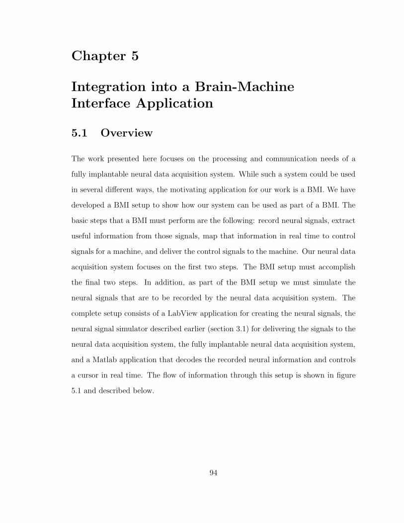
Chapter 5
Integration into a Brain-MachineInterface Application
5.1 Overview
The work presented here focuses on the processing and communication needs of a
fully implantable neural data acquisition system. While such a system could be used
in several different ways, the motivating application for our work is a BMI. We have
developed a BMI setup to show how our system can be used as part of a BMI. The
basic steps that a BMI must perform are the following: record neural signals, extract
useful information from those signals, map that information in real time to control
signals for a machine, and deliver the control signals to the machine. Our neural data
acquisition system focuses on the first two steps. The BMI setup must accomplish
the final two steps. In addition, as part of the BMI setup we must simulate the
neural signals that are to be recorded by the neural data acquisition system. The
complete setup consists of a LabView application for creating the neural signals, the
neural signal simulator described earlier (section 3.1) for delivering the signals to the
neural data acquisition system, the fully implantable neural data acquisition system,
and a Matlab application that decodes the recorded neural information and controls
a cursor in real time. The flow of information through this setup is shown in figure
5.1 and described below.
94
determine current direction of motion (based either on
predefined trajectory or "joystick" input)
compute instantaneous firing rate and then
generate spike times based on tuning curves
and refractory period
construct analog waveform based on spike times; send
through attenuator board to our system
system performs spike detection (and possibly sorting); outputs 50ms
bin counts
bin counts are sent to decoder, which in real- time maps bin counts to
direction
real-time reconstruction of trajectory is updated
bin counts
OR
estimate of current direction
Figure 5.1: Flow of information in the BMI setup.
95

5.2 Generating the Neural Waveforms
5.2.1 Spike Times
The underlying assumption behind the operation of a BMI is that information about
some parameter of interest is encoded in the neural signals. In BMI research, the
parameters of interest have often been related to motion – parameters such as po-
sition, direction, or velocity. For our BMI setup we have chosen to generate neural
waveforms that contain information about an angle. The decoded angle is ultimately
used to control the direction of motion of a cursor. For simplicity, we assume a con-
stant speed. Thus, a trajectory is completely defined by the evolution of the angle
versus time function. Information about the angle is encoded in firing rates. Each
unit’s firing rate is a cosine-tuned function of the difference between the current an-
gle and the unit’s preferred direction. Spike times for each unit are generated based
on the unit’s instantaneous firing rate as a function of time. We have two types of
trajectories that can be generated. A different method of determining spike times is
used for each one.
Predetermined Trajectory
One approach to generating the neural waveforms is to generate a complete trajectory
beforehand. Once the trajectory has been defined, the angle as a function of time
is known. We can then easily compute interspike intervals for a Poisson process (a
commonly used approximation for neural firing) using our knowledge of each unit’s
instantaneous firing rate [44]. The end result is that we have all of the spike times
for all of the units.
96

Real-time Control of Trajectory
An alternative to having a predetermined trajectory is to generate the trajectory in
real time. It is desirable to look at this case because it is more behaviorally relevant.
The contrast between a predetermined trajectory and real-time control of a trajectory
can be thought of as similar to the difference between a robot that is preprogrammed
to execute a fixed set of actions and a person using a mouse to follow a moving target
on a screen. We have implemented real-time control of the trajectory through the
use of a knob control on the front panel of the LabView application. The current
angle of motion at any instant in time is determined by the position of the knob at
that instant. Since the spike times encode information about the trajectory, we must
generate the spike times in real time as well. We do this by making a binary decision
regarding the presence of a spike every three milliseconds (based on the approximately
1 ms duration of a spike and a 2 ms refractory period). The probability of a spike
occurring for a unit during a given three millisecond period is based on the unit’s
instantaneous firing rate at that point in time.
5.2.2 Analog Waveforms
Ultimately, we want to generate analog waveforms that we can feed into our neu-
ral data acquisition system. A neural waveform can be thought of as consisting of
stereotypical spike shapes superimposed on background noise. Spikes from a single
unit will be similar in size and shape while spikes from different units may differ
significantly in size and shape. For the case of a predetermined trajectory, the Lab-
View application allows the user to select the standard deviation of the Gaussian
background noise. Spikes are then superimposed at the predetermined spike times.
The option of placing spikes from up to four units on a single waveform is available.
When multiple units are used to create a single waveform, spikes of different shapes
97

are used for each unit. The spike times for each unit are determined independently,
so overlapping spikes may be present in the final analog waveform. For the case in
which the trajectory is determined in real-time, we simplify the process of generating
analog waveforms since everything must be done in real time. No background noise
is added and each waveform is limited to having spikes from a single unit.
Once the full waveform is generated by the LabView application, the National
Instruments analog output card and the attenuator board are used to feed the neural
waveform into the neural data acquisition system.
5.3 Role of the Neural Data Acquisition System
The neural data acquisition system has already been described in detail. Within the
BMI setup, its role is to take the neural waveforms as input and to output either
sorted or unsorted 50-ms bin counts. This is the information that is then decoded
and used to control the cursor. These bin counts are sent from the WCM’s user
interface to the Matlab decoder application over a TCP connection.
5.4 Decoding and Cursor Control
A Matlab application maps the 50-ms bin counts that it receives to an angle. The
estimate of the current angle is simply computed as a weighted average of the es-
timated preferred directions of each of the units. The weights for any given 50-ms
period are proportional to the bin counts during that period. Clearly, estimations of
each unit’s preferred direction must be made before estimations of the current angle
can be made. Preferred directions are estimated during a training period in which
the Matlab application is receiving two types of information – the 50-ms bin counts
from the WCM’s user interface and the current angle from the waveform-generating
LabView application. Once all of the data for the training period have been col-
98

lected, a vector representing the preferred direction for each unit is computed. This
is done with a pseudoinverse matrix (using Matlab’s pinv function). The x- and
y-components of the preferred directions are computed as
xpd = pinv(bincounts) ∗ cos(angles)
ypd = pinv(bincounts) ∗ sin(angles)
where each column of the bincounts matrix holds the bin counts observed for a
given unit throughout the training period and angles is a column vector holding the
current angle for each of the 50-ms periods during the training period. xpd and ypd
are vectors holding the x- and y-components of the preferred directions of each of the
units. These preferred direction vectors are then used during the real-time decoding
phase to estimate the current angle. This estimate is made using
xest = xnormpd ∗ bincounts
yest = ynormpd ∗ bincounts
where the vector (xest, yest) represents the estimated direction for the current 50-ms
period, (xnormpd (i), ynorm
pd (i)) is a unit vector representing the preferred direction of unit
i, and bincounts is a row vector holding the bin counts observed for each of the units
during the current period.
As the angle is estimated for each 50-ms period, the position of a cursor in the
Matlab application is updated accordingly. This allows a user to watch as predeter-
mined trajectories are being reconstructed. In the case of real-time control of the
trajectory, the knob control indirectly (by means of affecting the generated neural
waveforms and consequently the angle estimations) controls the cursor on the Matlab
application. As a result, a user can use the knob control to guide the cursor to a
fixed target or to attempt to follow a moving target. Figure 5.2 shows a predeter-
mined trajectory and its reconstruction based on a total of 36 units across 15 different
99
channels. Figure 5.3 shows the real-time estimation of a trajectory controlled by the
joystick. Fifteen channels, each with a single unit, were used in this case. Note
that fairly good control of the estimated trajectory was achieved using the joystick
as indicated by our ability to write “duke.” Once again, it must be stated that the
position of the joystick does not directly control the estimated trajectory. Rather the
position of the joystick contains information that is encoded into the firing rates of
the analog waveforms generated by the neural simulator and used as input for our
neural data acquisition system. The estimated trajectory visible in the figure is the
result of decoding 50-ms bin counts output by our system.
5.5 BMI Setup as a Demonstration Platform
This BMI setup uses neither the most realistic means for simulating neural signals
nor the most sophisticated decoding algorithms. It must be remembered that the
focus of this work is the neural data acquisition system. The purpose of this BMI
setup is to demonstrate that the neural data acquisition system can work well within
the context of a BMI application. The BMI setup should be viewed as a platform for
demonstrating our system’s suitability for integration into a BMI application rather
than an in-depth piece of work in and of itself.
100

LabView application for creating neural signals
reconstructed trajectory
predetermined trajectory
Matlab application for reconstructing trajectories
raster plot of spike times for
each unit
Figure 5.2: This screenshot shows a LabView application that was used to create neural signals and a Matlab applicationthat was used to reconstruct trajectories in real time based on sorted bin counts. The reconstructed trajectory can beseen to match the true (i.e., “predetermined”) trajectory quite well.
101
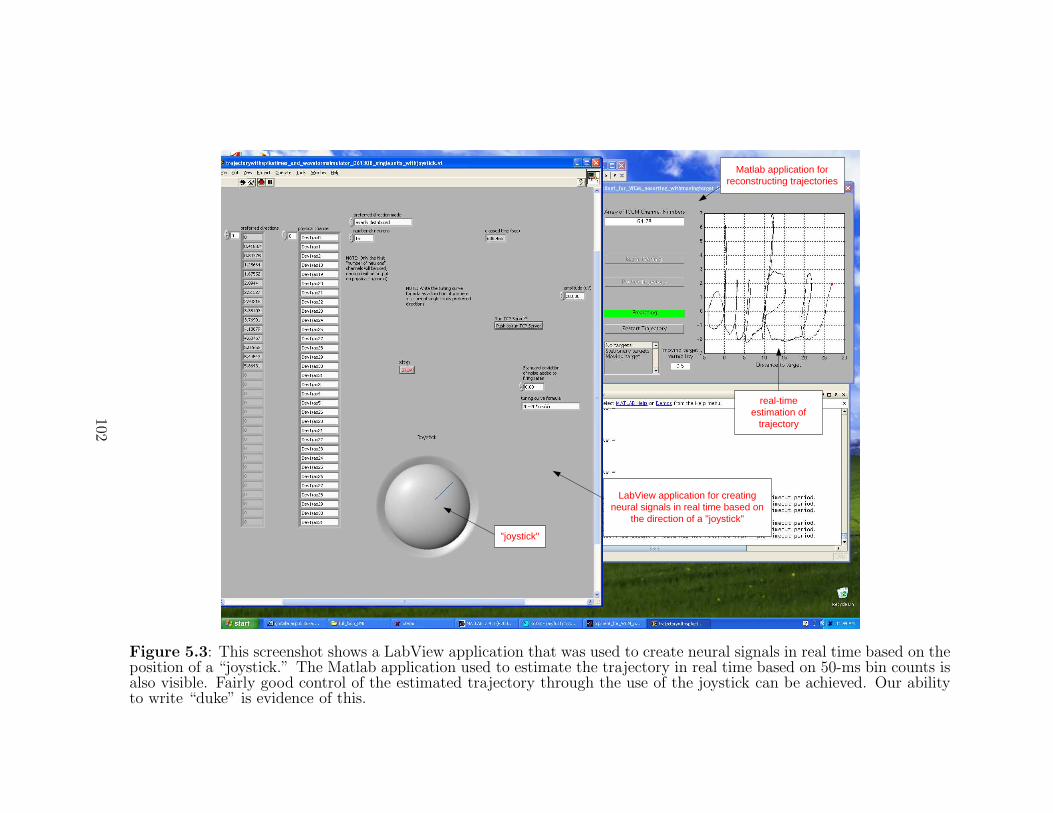
LabView application for creating neural signals in real time based on
the direction of a "joystick"
"joystick"
real-time estimation of
trajectory
Matlab application for reconstructing trajectories
Figure 5.3: This screenshot shows a LabView application that was used to create neural signals in real time based on theposition of a “joystick.” The Matlab application used to estimate the trajectory in real time based on 50-ms bin counts isalso visible. Fairly good control of the estimated trajectory through the use of the joystick can be achieved. Our abilityto write “duke” is evidence of this.
102
Chapter 6
Automatic Thresholding for SpikeDetection
This chapter takes an in-depth look at how to best set thresholds in fully implantable
neural data acquisition systems. We undertook a simulation study to compare and
evaluate various methods of automatically computing a threshold as a multiple of a
measure of the noise level. Our system, as well as others, uses this type of approach
(see section 2.2.1). This study confirms that the mean deviation operator is an
appropriate noise measure for use within our implantable neural signal processor.
The results also provide guidance regarding the selection of appropriate multipliers
for this means of spike detection.
6.1 Background
High channel-count fully implantable neural data acquisition systems must perform
data reduction before transmitting recorded neural data over a wireless link [47, 53,
65, 66]. However, these systems have significant size and power constraints and are
limited in the amount and complexity of processing that they can perform [73]. In
addition, timing constraints must be imposed on systems that are used in a real-
time application such as a BMI. Consequently, the use of amplitude thresholding for
spike detection is especially attractive for these systems due to its relative simplicity.
Voltage thresholding has been the method of choice for spike detection in recently
developed implantable neural signal processors [47, 53, 65, 66].
We have developed a 96-channel neural signal processor for use as part of a clinical
BMI [47]. The device automatically sets thresholds for each channel. The threshold
103

for a given channel is set to a multiple of an estimate of the noise level on that
channel. We would like to know how to best select thresholds within our implantable
neural signal processor. While several groups have used a multiple of some measure
of the noise level as a threshold, a few different noise measures have been used. The
most commonly used measure of noise is the root-mean-square (rms) of the data over
a given window, essentially the standard deviation of the data [55, 65, 74–79]. Other
noise measures that have been used are the mean deviation [47, 80] and the value of
the data located at a given percentile within a ranked set of data [81–83]. It must
be noted that all of the noise measures mentioned above do not measure only the
noise. In reality, they are calculated from the entire neural signal. The samples that
fall within a given window may simply be noise but they may also be spikes. So, the
distribution of the samples is dependent not only on the distribution of neural noise
but also on the size, shape, and number of spikes that fall within the window.
In order to effectively perform automatic threshold selection using a multiple of
a noise measure, we would like to select a single value of the multiplier and trust
that it will work reasonably well for all channels – even across channels that have
different firing rates and SNRs. So, we would like to know whether or not there is a
relatively consistent optimal multiplier for a given noise measure. A multiplier that
is near optimal across waveforms with varying characteristics would be suitable for
all channels in a high channel-count system such as ours.
This study investigates the problem of automatically selecting a threshold for spike
detection for use in an implantable neural signal processor. Thresholds computed
as multiples of four different noise measures are compared as SNR, firing rate, and
window size are varied. In addition, this study investigates the selection of an optimal
multiplier for each of these noise measures in neural waveforms that contain spikes
from either one or two neurons. While the results presented here are specific to a
104
particular method of spike detection, the concepts and optimization framework used
to perform the analysis are applicable more generally.
6.2 Methods
6.2.1 Simulated Waveforms
We compared the performance of thresholds computed as multiples of various noise
measures on simulated realistic neural signal waveforms. In order to simulate wave-
forms, we first constructed two libraries, one containing noise waveforms and the
other containing spike templates. The noise library contained 17 5-second segments
each from different channels of cortical microelectrode recordings from a rat. Each of
these segments had no visible spikes and was thus classified as noise. The recordings
were made with our system. Each data point was an 8-bit sample and the waveforms
were zero-mean. The spike template library consisted of 10 spike templates from rat
and monkey data recorded by our system. Each template was the average of similarly
shaped spikes extracted from a single channel.
For each simulated waveform, a 2-second span from one of the segments contained
in the noise library was randomly selected. A template was also randomly selected to
be used as the spike waveform to be inserted at locations within the 2-second noise
waveform. This method of simulating neural signals has been used widely throughout
the spike detection literature [54, 57, 60, 84, 85].
Each simulated waveform was described by two parameters – SNR and firing rate.
The SNR was used to scale the template. We define SNR as
SNR =peak amplitude of scaled template
standard deviation of 2-second noise waveform
(See section 6.4.7 for more on the definition of the SNR.) Spike times were selected to
determine where in the noise waveform to place the spike waveforms. For a given firing
105

rate, the appropriate number of spikes was placed into the waveform (for example,
for a firing rate of 20 Hz there would be 40 spikes in a 2-second waveform). Spike
times were randomly selected within the 2-second period; a refractory period of 1.6
ms was enforced. For each selected spike time, the spike waveform was added to the
noise waveform (resulting in a noisy version of the “clean” spike) with the portion
of the spike waveform with the highest amplitude placed at the selected spike time.
Thus, the simulation resulted in realistic neural waveforms with known SNRs and
spike times.
Rather than simulating an entirely new waveform (with a new noise waveform, a
new spike template, and completely new spike times) for each combination of SNR
and firing rate, sets of waveforms were simulated in a manner that limited all variation
due to factors other than changing SNRs or firing rates. Each set of waveforms was
generated in the following manner:
1. Randomly select a 2-second noise waveform.
2. Randomly select a spike template.
3. For the lowest firing rate of interest that has not yet been simulated, generate
spike times. If spike times have already been generated for lower firing rates,
start with those and generate more until the number of spikes corresponding
to the current firing rate has been generated.
4. For each SNR of interest, use the noise waveform, spike template, and spike
times to generate a full waveform.
5. If simulations have not yet been run for the highest firing rate of interest, go
back to step 3.
Figure 6.1 provides an example of a set of waveforms generated using this procedure.
106
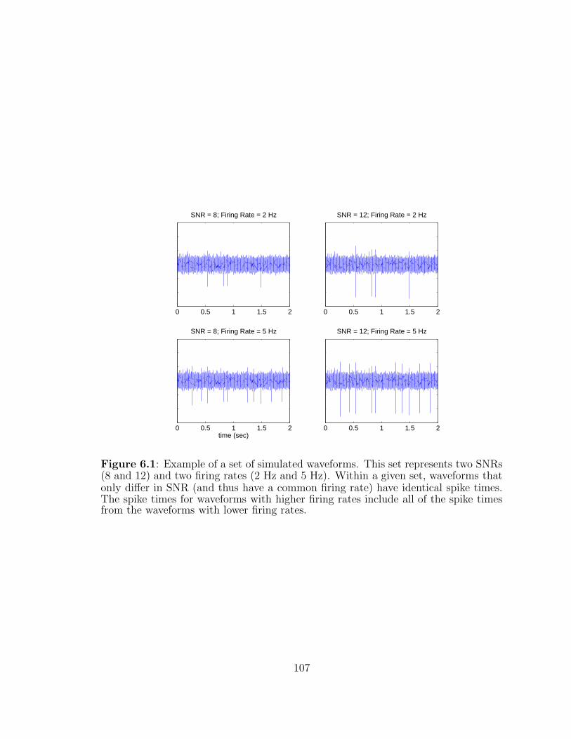
0 0.5 1 1.5 2
SNR = 8; Firing Rate = 2 Hz
0 0.5 1 1.5 2
SNR = 12; Firing Rate = 2 Hz
0 0.5 1 1.5 2time (sec)
SNR = 8; Firing Rate = 5 Hz
0 0.5 1 1.5 2
SNR = 12; Firing Rate = 5 Hz
Figure 6.1: Example of a set of simulated waveforms. This set represents two SNRs(8 and 12) and two firing rates (2 Hz and 5 Hz). Within a given set, waveforms thatonly differ in SNR (and thus have a common firing rate) have identical spike times.The spike times for waveforms with higher firing rates include all of the spike timesfrom the waveforms with lower firing rates.
107
The procedure described above generates neural waveforms that can be thought of
as containing spikes from a single neuron. Commonly, signals from multiple neurons
(or “units”) are observed on a single extracellularly recorded waveform. In order to
simulate this circumstance, we generated two-unit waveforms. This was done by first
simulating a single-unit waveform as described above. Then a second unit, with its
own SNR and firing rate, was added to the waveform. The spike times for the second
unit were selected independently of the spike times for the first unit. This created the
potential for overlapping spikes from different units, a phenomenon often observed
in real neural recordings. A template was scaled according to the SNR of the second
unit and spikes were added into the waveform at the selected times regardless of if
they overlapped with spikes from the first unit.
6.2.2 Noise Measures
For each simulated waveform, a sliding window was passed across the waveform and
at each point a noise measurement was made using four different operators – MD,
RMS, P84, and PA68. MD took the mean deviation of the points in the window.
Since the data were zero-mean, we simply took the mean of the absolute value of
the points in the window. RMS took the root-mean-square of all of the values in
the window. P84 found the 84th percentile of the data in the window. PA68 found
the 68th percentile of the absolute value of the data in the window. (For zero-mean,
normally distributed data, RMS, P84, and PA68 should approximate the standard
deviation of the data. MD should give σ√
2π
where σ is the standard deviation of the
data [86].)
These noise metrics are all based on measures that have been used throughout
the neural spike detection literature for setting thresholds (see section 6.1). For
108

zero-mean data, the operators are defined as follows:
MD(X) =1
N
N∑
i=1
|xi|
RMS(X) =
√
√
√
√
1
N
N∑
i=1
x2i
P84(X) = xbac + (xdae − xbac)(a − bac); a = 0.5 + 0.84N
PA68(X) = xbbc + (xdbe − xbbc)(b − bbc); b = 0.5 + 0.68N
where N is the window size; the vector X = {x1, . . . , xN} contains the waveform
samples that fall within the window; {x1, . . . , xN} contains the values in X sorted in
ascending order; {x1, . . . , xN} contains, in ascending order, the absolute values of the
elements in X; | · | is the absolute value function; b·c is the floor function; and d·e is
the ceiling function.
The size of the sliding window over which noise measures were computed was a
parameter that was varied.
6.2.3 Detection of Spikes
In order to perform spike detection, thresholds were applied to the absolute value
of the data. This method of spike detection has been shown to be appropriate for
computationally limited systems [48]. A refractory period of 1.28 ms (40 samples)
was imposed so that a single spike would not cause multiple detections. Detections
that occurred within 0.48 ms (15 samples) of the true spike time were considered to be
accurate detections. Detections falling outside of this time window were considered
to be false positives.
Thresholds were computed as multiples of the noise measures. A nonadaptive
threshold was computed for each position of the sliding window and applied to the
109
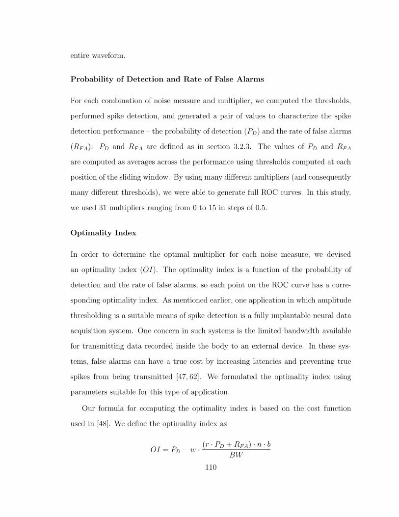
entire waveform.
Probability of Detection and Rate of False Alarms
For each combination of noise measure and multiplier, we computed the thresholds,
performed spike detection, and generated a pair of values to characterize the spike
detection performance – the probability of detection (PD) and the rate of false alarms
(RFA). PD and RFA are defined as in section 3.2.3. The values of PD and RFA
are computed as averages across the performance using thresholds computed at each
position of the sliding window. By using many different multipliers (and consequently
many different thresholds), we were able to generate full ROC curves. In this study,
we used 31 multipliers ranging from 0 to 15 in steps of 0.5.
Optimality Index
In order to determine the optimal multiplier for each noise measure, we devised
an optimality index (OI). The optimality index is a function of the probability of
detection and the rate of false alarms, so each point on the ROC curve has a corre-
sponding optimality index. As mentioned earlier, one application in which amplitude
thresholding is a suitable means of spike detection is a fully implantable neural data
acquisition system. One concern in such systems is the limited bandwidth available
for transmitting data recorded inside the body to an external device. In these sys-
tems, false alarms can have a true cost by increasing latencies and preventing true
spikes from being transmitted [47, 62]. We formulated the optimality index using
parameters suitable for this type of application.
Our formula for computing the optimality index is based on the cost function
used in [48]. We define the optimality index as
OI = PD − w ·(r · PD + RFA) · n · b
BW
110
where PD is the probability of detection, w is a unitless weight, r is the expected
firing rate per channel, RFA is the rate of false alarms per channel, n is the number
of channels, b is the number of bytes that will be transmitted for each detected spike,
and BW is the available bandwidth, or data rate, of the data acquisition system. The
second term of the formula represents the fraction of the available bandwidth that is
needed to transmit information about detections (whether true spikes or false alarms)
multiplied by the cost, w, of using all of the available bandwidth. Throughout this
study, we used 96 channels for n, 48 bytes per spike for b, and 96000 bytes per second
for BW . These values were taken from a 96-channel system that sends a channel
number, timestamp, and extracted spike waveform for each spike detected and has
a limited wireless data rate [47]. We also used a value of 50 spikes per channel per
second for r and a value of 0.1 for w.
In this study, we computed the optimality index separately for each SNR. This
allowed us to find an optimal multiplier for each noise measure for each SNR.
Optimality Score
We used the optimality score to find the optimal multiplier when all SNRs were taken
into consideration together. For a given multiplier, the optimality score is a weighted
average of the optimality indices at that multiplier and each of the SNRs. Table 6.1
presents the weights that we used. These weights correspond to the frequency with
which waveforms of a given SNR were found in a sample real neural recording. The
weights are based on the distribution of SNRs presented in figure 13 of [26]. This
figure contains histograms that show the distribution of SNRs observed on electrodes
implanted in the motor cortex for each of three monkeys. See section 6.4.7 for more
details on how the weights were determined.
111
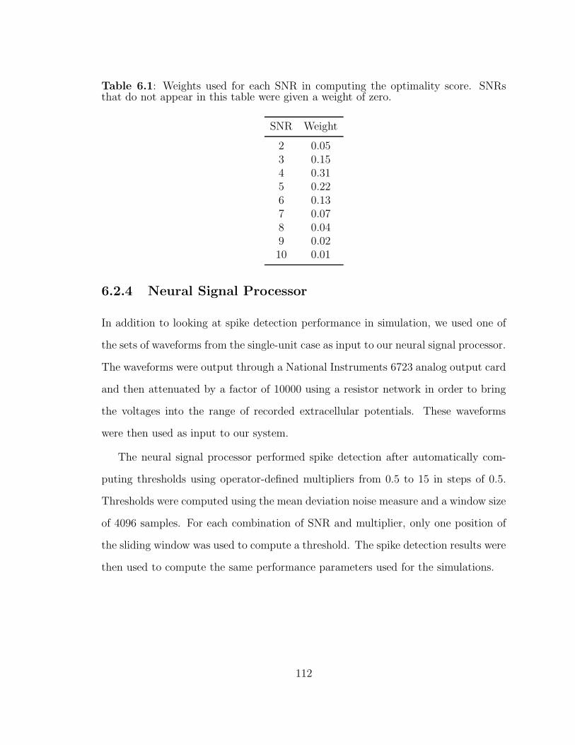
Table 6.1: Weights used for each SNR in computing the optimality score. SNRsthat do not appear in this table were given a weight of zero.
SNR Weight
2 0.053 0.154 0.315 0.226 0.137 0.078 0.049 0.0210 0.01
6.2.4 Neural Signal Processor
In addition to looking at spike detection performance in simulation, we used one of
the sets of waveforms from the single-unit case as input to our neural signal processor.
The waveforms were output through a National Instruments 6723 analog output card
and then attenuated by a factor of 10000 using a resistor network in order to bring
the voltages into the range of recorded extracellular potentials. These waveforms
were then used as input to our system.
The neural signal processor performed spike detection after automatically com-
puting thresholds using operator-defined multipliers from 0.5 to 15 in steps of 0.5.
Thresholds were computed using the mean deviation noise measure and a window size
of 4096 samples. For each combination of SNR and multiplier, only one position of
the sliding window was used to compute a threshold. The spike detection results were
then used to compute the same performance parameters used for the simulations.
112
6.3 Results
6.3.1 Single-Unit Waveforms
We simulated ten sets of waveforms. Each set had spikes from a single unit with
SNRs ranging from 1 to 15 in steps of 1 and firing rates ranging from 5 Hz to 50 Hz
in steps of 5 Hz. Each set of waveforms was generated as described in section 6.2.1.
On each waveform, we computed all four noise measures using window sizes of 512,
1024, 2048, 4096, and 8192 samples and performed spike detection as described in
section 6.2.3.
For the ten waveforms with a given SNR (from 1 to 15) and firing rate 20 Hz,
the probability of detection and rate of false alarms values were used to construct
optimality index curves for each of the four noise measures. These are plotted in
figure 6.2 as a function of the multiplier value. The plots are based on spike de-
tection performance using a window size of 4096 samples. The optimality indices
were computed using overall probabilities of detection and rates of false alarms mea-
sured across ten waveforms with identical firing rates and SNRs. Curves are plotted
for SNRs from 1 through 15. Figure 6.3(a) shows the maximum optimality index
achieved for each noise measure at each SNR and figure 6.3(b) shows the optimality
score for each multiplier for each noise measure. The multiplier that received the
highest optimality score for each noise measure is listed in table 6.2. Optimality
scores were also calculated for the other combinations of firing rate and window size.
Table 6.3 shows the maximum optimality score obtained for each noise measure for
selected parameter combinations. Overall, for a given set of parameters, compara-
ble maximum optimality scores were achieved by all of the noise measures for the
single-unit waveforms.
113
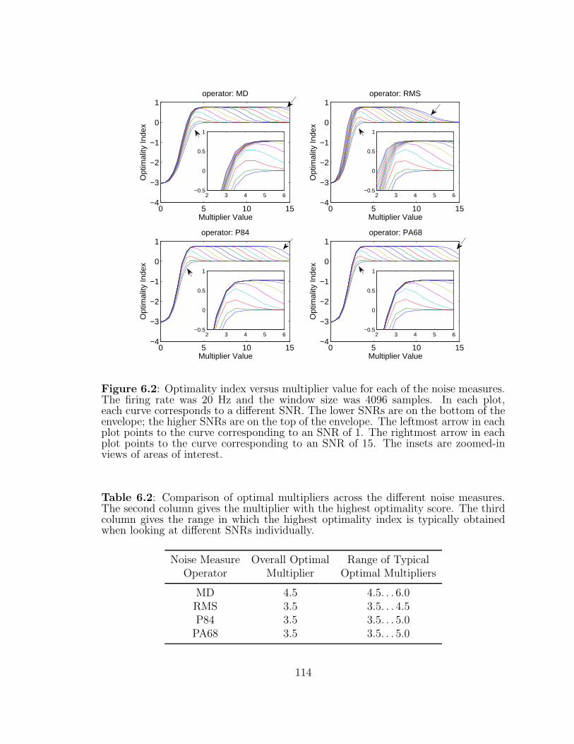
0 5 10 15−4
−3
−2
−1
0
1
Multiplier Value
Opt
imal
ity In
dex
operator: MD
2 3 4 5 6−0.5
0
0.5
1
0 5 10 15−4
−3
−2
−1
0
1
Multiplier Value
Opt
imal
ity In
dex
operator: RMS
2 3 4 5 6−0.5
0
0.5
1
0 5 10 15−4
−3
−2
−1
0
1
Multiplier Value
Opt
imal
ity In
dex
operator: P84
2 3 4 5 6−0.5
0
0.5
1
0 5 10 15−4
−3
−2
−1
0
1
Multiplier Value
Opt
imal
ity In
dex
operator: PA68
2 3 4 5 6−0.5
0
0.5
1
Figure 6.2: Optimality index versus multiplier value for each of the noise measures.The firing rate was 20 Hz and the window size was 4096 samples. In each plot,each curve corresponds to a different SNR. The lower SNRs are on the bottom of theenvelope; the higher SNRs are on the top of the envelope. The leftmost arrow in eachplot points to the curve corresponding to an SNR of 1. The rightmost arrow in eachplot points to the curve corresponding to an SNR of 15. The insets are zoomed-inviews of areas of interest.
Table 6.2: Comparison of optimal multipliers across the different noise measures.The second column gives the multiplier with the highest optimality score. The thirdcolumn gives the range in which the highest optimality index is typically obtainedwhen looking at different SNRs individually.
Noise Measure Overall Optimal Range of TypicalOperator Multiplier Optimal Multipliers
MD 4.5 4.5. . . 6.0RMS 3.5 3.5. . . 4.5P84 3.5 3.5. . . 5.0PA68 3.5 3.5. . . 5.0
114
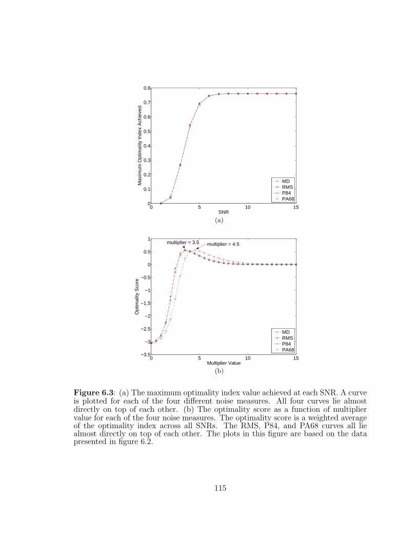
0 5 10 150
0.1
0.2
0.3
0.4
0.5
0.6
0.7
0.8
SNR
Max
imum
Opt
imal
ity In
dex
Ach
ieve
d
MDRMSP84PA68
(a)
0 5 10 15−3.5
−3
−2.5
−2
−1.5
−1
−0.5
0
0.5
1
Multiplier Value
Opt
imal
ity S
core
MDRMSP84PA68
multiplier = 3.5 multiplier = 4.5
(b)
Figure 6.3: (a) The maximum optimality index value achieved at each SNR. A curveis plotted for each of the four different noise measures. All four curves lie almostdirectly on top of each other. (b) The optimality score as a function of multipliervalue for each of the four noise measures. The optimality score is a weighted averageof the optimality index across all SNRs. The RMS, P84, and PA68 curves all liealmost directly on top of each other. The plots in this figure are based on the datapresented in figure 6.2.
115

Table 6.3: Maximum optimality score obtained for each operator for several com-binations of firing rate and window size. In each of these cases, the multiplier thatachieved the maximum was 4.5 for the MD operator and was 3.5 for each of the otherthree operators.
Firing Window Size MD RMS P84 PA68Rate (Hz) (samples)
5 512 0.5309 0.5275 0.5135 0.52185 4096 0.5381 0.5399 0.5370 0.53685 8192 0.5380 0.5402 0.5392 0.537520 512 0.5424 0.5394 0.5245 0.532920 4096 0.5528 0.5574 0.5487 0.548620 8192 0.5534 0.5581 0.5508 0.550050 512 0.5455 0.5418 0.5365 0.544250 4096 0.5573 0.5611 0.5586 0.558550 8192 0.5576 0.5619 0.5594 0.5591
6.3.2 Two-Unit Waveforms
We simulated two-unit waveforms in which the first unit had an SNR of 8 and each
unit had a firing rate of 20 Hz. For each set of waveforms, the SNR of the second
unit was varied from 1 to 8 in steps of 1. Ten of these sets were simulated. Similar to
section 6.3.1, spike detection was performed and optimality indices and scores were
computed. These results are shown in figure 6.4. Since the SNR of the first unit
was held constant at a value of 8, all variations in SNR referred to in the plots and
calculations correspond to the SNR of the second unit.
Similarly, we also simulated two-unit waveforms in which the first unit had an
SNR of 12. The results for this case are shown in figure 6.5.
6.3.3 Neural Signal Processor
The spike detection results for our neural signal processor are shown in figure 6.6.
Two points must be noted regarding these results. First, only one threshold (based on
a randomly selected position of the sliding window) was used for each combination
116
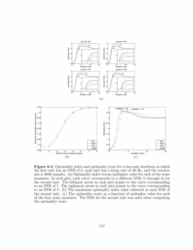
0 5 10 15−3
−2
−1
0
1
Multiplier ValueO
ptim
ality
Inde
x
operator: MD
2 3 4 50
0.5
1
0 5 10 15−3
−2
−1
0
1
Multiplier Value
Opt
imal
ity In
dex
operator: RMS
2 3 4 50
0.5
1
0 5 10 15−3
−2
−1
0
1
Multiplier Value
Opt
imal
ity In
dex
operator: P84
2 3 4 50
0.5
1
0 5 10 15−3
−2
−1
0
1
Multiplier Value
Opt
imal
ity In
dex
operator: PA68
2 3 4 50
0.5
1
(a)
1 2 3 4 5 6 7 80.35
0.4
0.45
0.5
0.55
0.6
0.65
0.7
0.75
SNR for lower amplitude signal
Max
imum
Opt
imal
ity In
dex
Ach
ieve
d
MDRMSP84PA68
(b)
0 5 10 15−3
−2.5
−2
−1.5
−1
−0.5
0
0.5
1
Multiplier Value
Opt
imal
ity S
core
MDRMSP84PA68
multiplier = 3.5 multiplier = 4.5
(c)
Figure 6.4: Optimality index and optimality score for a two-unit waveform in whichthe first unit has an SNR of 8, each unit has a firing rate of 20 Hz, and the windowsize is 4096 samples. (a) Optimality index versus multiplier value for each of the noisemeasures. In each plot, each curve corresponds to a different SNR (1 through 8) forthe second unit. The leftmost arrow in each plot points to the curve correspondingto an SNR of 1. The rightmost arrow in each plot points to the curve correspondingto an SNR of 8. (b) The maximum optimality index value achieved at each SNR ofthe second unit. (c) The optimality score as a function of multiplier value for eachof the four noise measures. The SNR for the second unit was used when computingthe optimality score.
117
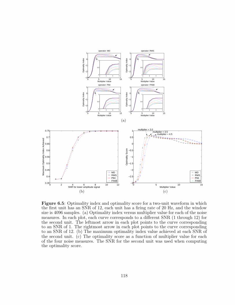
0 5 10 15−3
−2
−1
0
1
Multiplier ValueO
ptim
ality
Inde
x
operator: MD
2 3 4 50
0.5
1
0 5 10 15−3
−2
−1
0
1
Multiplier Value
Opt
imal
ity In
dex
operator: RMS
2 3 4 50
0.5
1
0 5 10 15−3
−2
−1
0
1
Multiplier Value
Opt
imal
ity In
dex
operator: P84
2 3 4 50
0.5
1
0 5 10 15−3
−2
−1
0
1
Multiplier Value
Opt
imal
ity In
dex
operator: PA68
2 3 4 50
0.5
1
(a)
0 2 4 6 8 10 120.35
0.4
0.45
0.5
0.55
0.6
0.65
0.7
0.75
SNR for lower amplitude signal
Max
imum
Opt
imal
ity In
dex
Ach
ieve
d
MDRMSP84PA68
(b)
0 5 10 15−3
−2.5
−2
−1.5
−1
−0.5
0
0.5
1
Multiplier Value
Opt
imal
ity S
core
MDRMSP84PA68
multiplier = 3.0multiplier = 3.5
multiplier = 4.5
(c)
Figure 6.5: Optimality index and optimality score for a two-unit waveform in whichthe first unit has an SNR of 12, each unit has a firing rate of 20 Hz, and the windowsize is 4096 samples. (a) Optimality index versus multiplier value for each of the noisemeasures. In each plot, each curve corresponds to a different SNR (1 through 12) forthe second unit. The leftmost arrow in each plot points to the curve correspondingto an SNR of 1. The rightmost arrow in each plot points to the curve correspondingto an SNR of 12. (b) The maximum optimality index value achieved at each SNR ofthe second unit. (c) The optimality score as a function of multiplier value for eachof the four noise measures. The SNR for the second unit was used when computingthe optimality score.
118
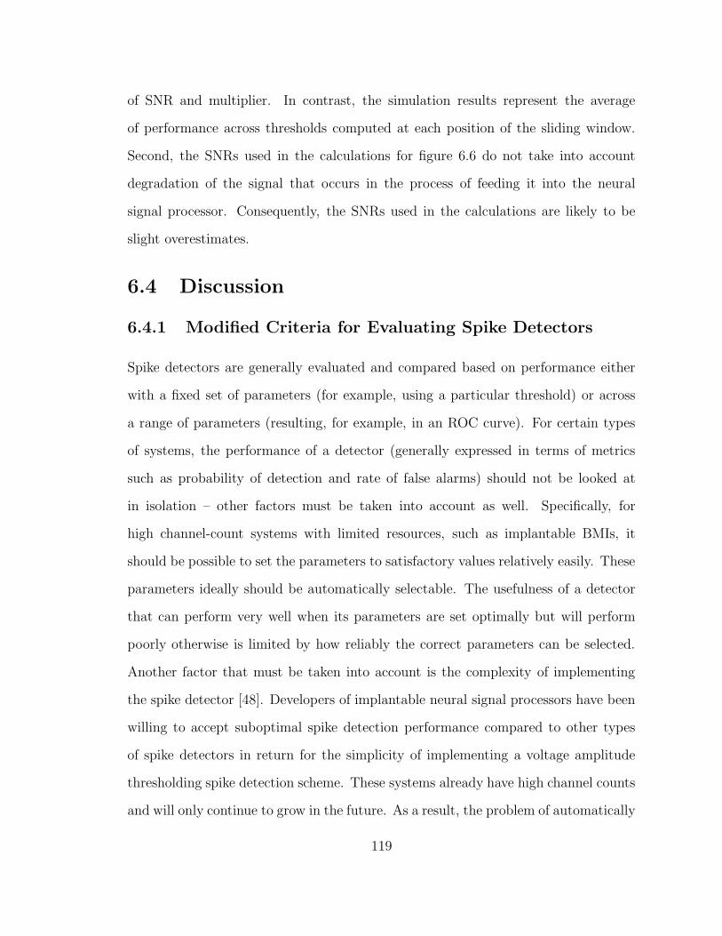
of SNR and multiplier. In contrast, the simulation results represent the average
of performance across thresholds computed at each position of the sliding window.
Second, the SNRs used in the calculations for figure 6.6 do not take into account
degradation of the signal that occurs in the process of feeding it into the neural
signal processor. Consequently, the SNRs used in the calculations are likely to be
slight overestimates.
6.4 Discussion
6.4.1 Modified Criteria for Evaluating Spike Detectors
Spike detectors are generally evaluated and compared based on performance either
with a fixed set of parameters (for example, using a particular threshold) or across
a range of parameters (resulting, for example, in an ROC curve). For certain types
of systems, the performance of a detector (generally expressed in terms of metrics
such as probability of detection and rate of false alarms) should not be looked at
in isolation – other factors must be taken into account as well. Specifically, for
high channel-count systems with limited resources, such as implantable BMIs, it
should be possible to set the parameters to satisfactory values relatively easily. These
parameters ideally should be automatically selectable. The usefulness of a detector
that can perform very well when its parameters are set optimally but will perform
poorly otherwise is limited by how reliably the correct parameters can be selected.
Another factor that must be taken into account is the complexity of implementing
the spike detector [48]. Developers of implantable neural signal processors have been
willing to accept suboptimal spike detection performance compared to other types
of spike detectors in return for the simplicity of implementing a voltage amplitude
thresholding spike detection scheme. These systems already have high channel counts
and will only continue to grow in the future. As a result, the problem of automatically
119
0 5 10 15−4
−3.5
−3
−2.5
−2
−1.5
−1
−0.5
0
0.5
1
Multiplier Value
Opt
imal
ity In
dex
(a)
0 5 10 150
0.1
0.2
0.3
0.4
0.5
0.6
0.7
0.8
SNR
Max
imum
Opt
imal
ity In
dex
Ach
ieve
d
(b)
0 5 10 15−3.5
−3
−2.5
−2
−1.5
−1
−0.5
0
0.5
1
Multiplier Value
Opt
imal
ity S
core
multiplier = 4.5
(c)
Figure 6.6: Optimality index and optimality score representing the spike detectionperformance of our neural signal processor. The firing rate was 20 Hz and the neuralsignal processor used a window size of 4096 samples. (a) Optimality index versusmultiplier value. Each curve corresponds to a different SNR (1 through 15). Theleftmost arrow points to the curve corresponding to an SNR of 1. The rightmost arrowpoints to the curve corresponding to an SNR of 15. (b) The maximum optimalityindex value achieved at each SNR. (c) The optimality score as a function of multipliervalue.
120

selecting thresholds is an important one. Spike detectors for these systems should
be evaluated not only on their achievable levels of performance, but also on their
complexity and ability to perform well using parameters that are selected without
supervision.
6.4.2 Threshold Stability
Neural data is often thought of as consisting of large amplitude spikes superimposed
on a noise cloud primarily representing background neural activity. Calculations that
use a portion of the recorded data to estimate the noise level will be affected by spikes
that happen to fall within the window over which the calculation is made. The level
to which the calculation is affected depends on the firing rate and SNR of the spikes
as well as the type of calculation.
A relatively straightforward way to automatically compute a threshold is to use a
multiple of a noise measure as the threshold. In this case, having a relatively stable
noise measure is desirable. Thresholds calculated based on the noise measure made
during an initial monitoring period ideally should not be significantly influenced by
the location in time at which the monitoring period occurs (since that is essentially
random).
6.4.3 Optimal Multipliers for Single-Unit Waveforms
Having to select a multiplier for each channel individually essentially defeats the
purpose of trying to automatically set thresholds. If an individual is required to look
at each channel in order to choose the multiplier, he might as well directly set the
threshold for each channel. It is valuable to know the range over which multipliers
are near optimal for waveforms with different firing rates and SNRs. This way a
multiplier that can perform well across many channels can be selected. There can
121
still be some design flexibility in picking the multiplier. A value toward the high
end of the range would limit false detections and a value toward the low end would
increase the probability of detection. At the same time, it is desirable to have a wide
range of multipliers that are near optimal so that performance will not suffer greatly
as long as a multiplier near the optimal multiplier is used. We used the optimality
index described in section 6.2.3 and computed in section 6.3.1 to compare the optimal
multipliers for the different noise measures.
From figure 6.2 it is clear that for a given noise measure, the optimality index can
reach its peak at slightly different multiplier values for different SNRs. As a result, a
single optimal multiplier cannot be identified. Nevertheless, across SNRs the optimal
multiplier does generally fall within a small range. These ranges are different for the
different noise measures (table 6.2). In order to pick a single multiplier to be used
across channels with a variety of SNRs, an optimality score that is computed using
weights corresponding to the frequency with which a given SNR occurs is appropriate.
While the optimality index curves shown in figure 6.2 look relatively similar for
the different noise measures, one noticeable difference is the range over which the
individual curves remain near their peaks. Curves remain near their peaks over
the widest range for the MD operator. The range is slightly narrower for the P84
and PA68 operators. Finally, for the RMS operator, the range is even narrower.
A review of the literature shows that many different multipliers have been used
[47, 55, 65, 74, 76–79,81–83]. In some cases these may not have been optimal.
6.4.4 Effect of Multiple Units
While the spike detection performance of all four operators was quite similar for
waveforms containing spikes from only one unit, a couple of interesting observations
can be made regarding the performance for waveforms containing spikes from two
122

units. First, when large amplitude spikes from one unit are present along with lower
amplitude spikes from a second unit, the maximum optimality indices achieved by the
RMS operator at the SNRs that are most common (SNRs of 3 through 6 according
to table 6.1) are lower than those achieved by the other operators. (Compare figures
6.4(b) and 6.5(b) with figure 6.3(a).) Second, the optimality score curve for the RMS
operator peaks farther to the left (at a lower multiplier value) in the two-unit case
than it does in the single-unit case. This can be seen by comparing figures 6.3(b)
and 6.5(c). For the other operators, the multiplier for which the optimality score is
highest remained unchanged across all of the different parameter combinations and
circumstances investigated. This suggests that a single multiplier may prove to be
optimal more generally for the MD, P84, and PA68 operators than for the RMS
operator.
6.4.5 Comparison of Noise Measures
The complexity of neural noise should not be underestimated. It has been observed
to be colored and non-stationary [57, 87]. The complexity of the neural waveforms
over which noise calculations are performed is further complicated by the presence of
spikes in addition to the noise. These spikes distort the distribution of the samples
in the waveform since they contain a disproportionate number of high amplitude
samples [61]. As a result, the noise level estimates (and consequently the thresholds)
computed by the different noise measures should not automatically be assumed to
lead to equal performance as they might when applied to large samples of simple,
perfectly Gaussian data. Since the statistical nature of the overall neural waveform
is not simple or obvious, an experimental approach (using real data as opposed to a
statistical model) to the problem under consideration is warranted.
While the overall performance of all four measures investigated in this study
123
was fairly similar, the root-mean-square operator did exhibit a few disadvantageous
characteristics. The range of multipliers over which a given optimality index curve
remained near its peak was narrowest for the RMS operator (section 6.4.3). In the
two-unit case, the RMS operator had lower maximum optimality indices and a less
consistent optimal multiplier than the other operators (section 6.4.4). Additionally,
performing the squaring and square root operations used by the RMS operator can
be problematic in certain types of systems. This suggests that using a percentile
operator may be preferable for a system utilizing a mixed-signal processor [81, 83]
and using the mean deviation operator may be preferable for a system utilizing a
digital processor with limited memory resources [47].
6.4.6 Limitations and Extensions
It should be noted that the results presented in section 6.3 and discussed in sections
6.4.3 and 6.4.4 use a specific value of the weight w. This weight is related to the
cost incurred by false detections. False detections can range from simply being a
nuisance to causing a severe drop in performance depending on the circumstances.
For example, in a wired recording system in which spikes are detected and extracted
with essentially no limit on the number of spikes and in which a reliable spike sorting
process will be performed (meaning that most of the false extractions will later be
categorized as noise rather than as true spikes), false detections are undesirable but
should have only a minor impact on the performance of the system. In this case,
the emphasis should be on picking a multiplier that results in a high probability of
detection.
In the case of a fully implantable neural data acquisition system with a limited
data rate, false detections will take up valuable bandwidth and could possibly prevent
some true spikes from being transmitted [47]. Even if spike sorting is performed
124
after the extracted spikes are received outside of the body (again categorizing false
detections as noise), some of the true spiking information may be irretrievably lost
due to the false detections. The cost of false detections might be relatively high in
this case if the data rate necessary for true spikes is close to the available data rate.
Another case is a system that does not use spike sorting but instead simply pro-
cesses spike detection information. This system would end up treating false detections
exactly like true spikes. Thus false detections would never be removed and the per-
formance of the system could be impacted negatively. In this case, multipliers that
lead to many false detections would not be considered optimal.
From these examples it is clear that the multiplier that is considered to be optimal
in one case may not be considered optimal in another. In this study, we looked at
one possible case.
Also, this study, as all studies must, had a limited scope. Seemingly endless com-
binations of SNRs, firing rates, and window sizes could have been investigated, espe-
cially when allowing spikes from multiple neurons to be present in a given waveform.
This study investigated only a limited subset of the possible parameter combinations.
Nevertheless, many of the ideas and methods presented here can be extended and
applied to circumstances and spike detection techniques that do not exactly match
those presented in this study. For example, we found that the results using an adap-
tive threshold were very similar to the average performance of nonadaptive thresholds
presented here.
Also, this work is applicable beyond the realm of implantable neural data acqui-
sition systems. Voltage thresholding is used widely to perform neural spike detec-
tion in many different contexts [17, 47, 53, 55, 65, 66, 74–83, 88–90]. Other means of
spike detection exist and have the potential to have improved spike detection perfor-
mance [54, 56–58, 61, 85, 91–95]. Nevertheless, voltage amplitude thresholding, even
125

with its less than ideal spike detection performance, is the predominant method of
spike detection. This is in large part due to its simplicity and its ease of implemen-
tation. Automatic threshold selection is desirable in a wide variety of circumstances.
Finally, we suggest that the ability to easily and robustly select parameters that
result in good performance across a wide range of realistic circumstances should
be considered while developing and evaluating spike detection techniques. This is
especially true for spike detection techniques intended for use in implantable systems.
The optimization framework presented here may be useful in the development and
evaluation of many of these techniques.
6.4.7 Final Notes
SNR
No consistent definition of SNR is found in the neural spike processing literature.
Two commonly used definitions are the one used here (see section 6.2.1) [57, 79, 85]
and one in which the numerator of the ratio is the rms value of the template rather
than the peak amplitude of the template [54,55,59,61,96]. Other definitions are used
as well [26, 56, 58, 60, 95]. A definition of SNR that relies on the peak amplitude fits
well with a detection scheme that uses an amplitude threshold since only the high
amplitude portion of the spike is likely to cross the threshold and lead to a detection.
Also, SNR computations that rely on the rms value of a spike are influenced by the
assumed temporal duration of the spike. In general, exactly what portion of a full
neural waveform should be considered to be part of a spike is not well-defined. For a
useful note on SNR see [57].
The difference in how SNR is defined here and in [26] must specifically be men-
tioned. In [26], SNR is defined as the peak-to-peak amplitude of the spikes divided
by two times the standard deviation of the noise. The spike templates used in our
126
study had, on average, peak-to-peak amplitudes that were approximately 1.5 times
the size of their peak amplitudes. In order to account for this, we scaled the SNR
values presented in [26] by 43
so that they would correspond to the SNR values used
here. Once this was done, we used the frequency with which waveforms of a given
SNR were found in the recordings from [26] to determine the weights used in the
optimality score calculation.
Spike Detection Performance Parameters
In section 6.2.3, we characterize the spike detection performance by two parameters
– PD and RFA. In the spike detection literature, it is more common to plot PD versus
the probability of false alarm (PFA) or the “false alarm ratio” [56–58, 60, 88]. These
are generally defined as the number of false alarms divided by the total number of
detections. We feel that RFA is a more appropriate measure because it is essentially
independent of the firing rate of the spike whereas PFA, as it is generally defined, is
very dependent on the firing rate. In a rough sense, for a given threshold, RFA can be
thought of as a measure of the noise level and PD can be thought of as a measure of
the signal level, both independent of firing rate. While plots of PD versus RFA do not
exactly correspond to classical ROC curves, they do present the same general type of
information. A few others have also plotted the probability of detection versus the
rate of false alarms [95, 97].
127
Chapter 7
Conclusion
We have addressed problems related to reduction, telemetry, and processing of neu-
ral data for a fully implantable data acquisition system. Specifically, we have imple-
mented data reduction algorithms within an implantable module, developed a wireless
communications link between the implantable module and an external module, and
enabled the external module to perform real-time spike sorting. We have evaluated
the neural signal processing performed by our system on the bench and investigated
appropriate means for performing spike detection in an implantable neural signal pro-
cessor. Finally, we have confirmed that the telemetry and processing aspects of our
system function properly as part of a fully implanted system. This work demonstrates
that the fundamental neural data acquisition and processing tasks that have proven
to be effective within the laboratory environment using percutaneous systems can be
performed by a fully implantable system. Our demonstration of a neural data ac-
quisition system that effectively acquires, transmits, and processes neural data while
fully implanted creates a clearer path for future clinical applications of neural data
acquisition systems.
This work has been approached with an eye toward the use of a fully implantable
neural data acquisition system as part of a clinically viable BMI. Our focus has been
on the processing performed within our system, and we have presented this work
within the context of the full neural data acquisition system and the BMI application.
The overall development of our fully implantable neural data acquisition system has
not been nicely and neatly wrapped up. There are many areas in which our system
can be improved. The goal of this work, however, was to recognize and address some
128

(not all) of the challenges that stand in the way of using a neural data acquisition
system in a clinical setting. A recent review stated that “the issues related to the
long-term functionality of implantable microelectrodes, and to the development of
fully implantable electronic devices for amplification of a large number or neuronal
signals and their wireless transmission to the actuator, are the major technological
challenges that will determine the success or failure of future clinical applications of
BMI technology” [1]. This work has pushed us closer to overcoming the obstacles
standing in the way of a clinical BMI.
A future clinical BMI might take one of several different forms, and depending on
its form will require different features. Much of the work presented here centers on
the idea of relaying neural information from inside the body to the external world.
This ability is required when the end goal is to control an external machine such as
a wheelchair or a computer. It is conceivable that a closed loop BMI requiring no
external processing and no interaction with an external machine could be developed.
In this case, there may never be a need to send the neural data out of the body.
Nevertheless, much of the processing presented in this work is still applicable to such
a case. Finally, the work presented here is also applicable outside of the realm of
BMIs. As mentioned before, neural data acquisition is quite common within the
research world. Significant effort has been put forth to make wired recording sys-
tems suitable for recording from freely behaving animals [98]. The wireless recording
system presented here (whether implanted or not) may be beneficial in these types
of research environments. We hope that this work will prove to be beneficial in a
variety of circumstances in which neural data acquisition is performed.
129

Bibliography
[1] M A Lebedev and M A Nicolelis. Brain-machine interfaces: past, present andfuture. Trends Neurosci, 29(9):536–546, Sep 2006.
[2] J K Chapin. Using multi-neuron population recordings for neural prosthetics.Nat Neurosci, 7(5):452–455, May 2004.
[3] J T McIlwain. Population coding: a historical sketch. In M A L Nicolelis, editor,Advances in Neural Population Coding. Elsevier Science B.V., Amsterdam, 2001.
[4] A A Ghazanfar, C R Stambaugh, and M A L Nicolelis. Encoding of tactilestimulus location by somatosensory thalamocortical ensembles. J Neurosci,20(10):3761–3775, May 2000.
[5] J Wessberg, C R Stambaugh, J D Kralik, P D Beck, M Lauback, J K Chapin,J Kim, S J Biggs, M A Srinivasan, and M A L Nicolelis. Real-time prediction ofhand trajectory by ensembles of cortical neurons in primates. Nature, 408:361–365, Nov 2000.
[6] J M Carmena, M A Lebedev, R E Crist, J E O’Doherty, D M Santucci, D FDimitrov, P G Patil, C S Henriquez, and M A Nicolelis. Learning to controla brain-machine interface for reaching and grasping by primates. PLoS Biol,1(2):193–208, Nov 2003.
[7] S J Kim, S C Manyam, D J Warren, and R A Normann. Electrophysiologicalmapping of cat primary auditory cortex with multielectrode arrays. Ann BiomedEng, 34(2):300–309, Feb 2006.
[8] S D Van Hooser, J A Heimel, S Chung, and S B Nelson. Lack of patchy horizontalconnectivity in primary visual cortex of a mammal without orientation maps. JNeurosci, 26(29):7680–7692, Jul 2006.
[9] M J Lehmkuhle, R A Normann, and E M Maynard. High-resolution analysis ofthe spatio-temporal activity patterns in rat olfactory bulb evoked by enantiomerodors. Chem Senses, 28:499–508, Jul 2003.
[10] D M Santucci, J D Kralik, M A Lebedev, and M A L Nicolelis. Frontal andparietal cortical ensembles predict single-trial muscle activity during reachingmovements in primates. Eur J Neurosci, 22:1529–1540, Sep 2005.
[11] R Q Quiroga, L Reddy, G Kreiman, C Kock, and I Fried. Invariant visualrepresentation by single neurons in the human brain. Nature, 435:1102–1107,Jun 2005.
130
[12] M D Serruya, N G Hatsopoulos, L Paninski, M R Fellows, and J P Donoghue.Instant neural control of a movement signal. Nature, 416(6877):141–142, Mar2002.
[13] D M Taylor, S I Tillery, and A B Schwartz. Direct cortical control of 3d neuro-prosthetic devices. Science, 296(5574):1829–1832, Jun 2002.
[14] L R Hochberg, M D Serruya, G M Friehs, J A Mukand, M Saleh, A H Caplan,A Branner, D Chen, R D Penn, and J P Donoghue. Neuronal ensemble controlof prosthetic devices by a human with tetraplegia. Nature, 442(7099):164–171,Jul 2006.
[15] E M Schmidt. Electrodes for many single neuron recordings. In M A L Nicolelis,editor, Methods for Neural Ensemble Recordings. CRC Press, Boca Raton, 1999.
[16] K A Moxon. Multichannel electrode design: considerations for different appli-cations. In M A L Nicolelis, editor, Methods for Neural Ensemble Recordings.CRC Press, Boca Raton, 1999.
[17] M A Nicolelis, D Dimitrov, J M Carmena, R Crist, G Lehew, J D Kralik, andS P Wise. Chronic, multisite, multielectrode recordings in macaque monkeys.Proc Natl Acad Sci USA, 100(19):11041–11046, Sep 2003.
[18] R E Isaacs, D J Weber, and A B Schwartz. Work toward real-time control of acortical neural prosthesis. IEEE Trans Rehabil Eng, 8(2):196–198, Jun 2000.
[19] D C Bradley, P R Troyk, J A Berg, M Bak, S Cogan, R Erickson, C Kufta,M Mascaro, D McCreery, E M Schmidt, V L Towle, and H Xu. Visuotopic map-ping through a multichannel stimulating implant in primate V1. J Neurophysiol,93:1659–1670, 2005.
[20] Inc Plexon, Sep 2006. http://www.plexoninc.com/MAP.htm.
[21] Inc Plexon. Map system data sheet, Sep 2006.http://www.plexoninc.com/pdf/Plexon MAP Datasheet.pdf.
[22] I Obeid, M A L Nicolelis, and P D Wolf. A multichannel telemetry system forsingle unit neural recordings. J Neurosci Methods, 133:33–38, Feb 2004.
[23] J Mavoori, A Jackson, C Diorio, and E Fetz. An autonomous implantable com-puter for neural recording and stimulation in unrestrained primates. J NeurosciMethods, 148:71–77, Oct 2005.
[24] J Morizio, P Irazoqui, V Go, and J Parmentier. Wireless headstage for neuralprosthetics. Proc 2nd Int IEEE EMBS Conf Neural Eng, pages 414–417, Mar2005.
131

[25] M D Linderman, V Gilja, G Santhanam, A Afshar, S Ryu, T H Meng, and K VShenoy. An autonomous, broadband, multi-channel neural recording system forfreely behaving primates. Proc 28th IEEE EMBS Annu Int Conf, pages 1212–1215, Aug/Sep 2006.
[26] S Suner, M R Fellows, C Vargas-Irwin, G K Nakata, and J P Donoghue. Re-liability of signals from a chronically implanted, silicon-based electrode arrayin non-human primate primary motor cortex. IEEE Trans Neural Syst RehabilEng, 13(4):524–541, Dec 2005.
[27] M A L Nicolelis, C R Stambaugh, A Brisben, and M Laubach. Methods forsimultaneous multisite neural ensemble recordings in behaving primates. InM A L Nicolelis, editor, Methods for Neural Ensemble Recordings. CRC Press,Boca Raton, 1999.
[28] K A Moxon, J C Morizio, J K Chapin, M A Nicolelis, and P Wolf. Design-ing a brain-machine interface for neuroprosthetic control. In J K Chapin andK A Moxon, editors, Neural Prostheses for Restoration of Sensory and MotorFunction. CRC Press, Boca Raton, FL, 2001.
[29] W Greatbatch and C F Holmes. History of implantable devices. IEEE Eng MedBiol, 10(3):38–41,49, Sep 1991.
[30] P J Hendry, T V Mussivand, R G Masters, M E Bourke, G M Guiraudon, K SHolmes, K D Day, and W J Keon. The HeartSaver left ventricular assist device:an update. Ann Thorac Surg, 71(3):S166–S170, Mar 2001.
[31] K Au-Yeung, C R Johnson, and P D Wolf. A novel implantable cardiac telemetrysystem for studying atrial fibrillation. Physiol Meas, 25(5):1223–1238, Oct 2004.
[32] L Wang, E A Johannessen, P A Hammond, L Cui, S W J Reid, J M Cooper,and D R S Cumming. A programmable microsystem using system-on-chip forreal-time biotelemetry. IEEE Trans Biomed Eng, 52(7):1251–1260, Jul 2005.
[33] C Liang, J J Chen, C Chung, C Cheng, and C Wang. An implantable bi-directional wireless transmission system for transcutaneous biological signalrecording. Physiol Meas, 26:83–97, Feb 2005.
[34] W G Scanlon, J B Burns, and N E Evans. Radiowave propagation from atissue-implanted source at 418 MHz and 916.5 MHz. IEEE Trans Biomed Eng,47(4):527–534, Apr 2000.
[35] S Haykin. Communication Systems. John Wiley and Sons, Inc., 2001.
[36] M Ahmadian, B W Flynn, A F Murray, and D R S Cumming. Data transmissionfor implantable microsystems using magnetic coupling. IEE Proc - Commun,152(2):247–250, Apr 2005.
132

[37] K S Guillory, A K Misener, and A Pungor. Hybrid rf/ir transcutaneous telemetryfor power and high-bandwidth data. In Proc 26th Annu Int Conf IEEE EMBS,volume 2, pages 4338–4340, Sep 2004.
[38] K R Foster and H P Schwan. Dielectric properties of tissues. In C Polk andE Postow, editors, Handbook of Biological Effects of Electromagnetic Fields. CRCPress, Boca Raton, 1996.
[39] F A Duck. Physical Properties of Tissue: A Comprehensive Reference Book.Academic Press, 1990.
[40] U S Inan and A S Inan. Electromagnetic Waves. Prentice Hall, 2000.
[41] J C Lin and O P Gandhi. Computational methods for predicting field intensity.In C Polk and E Postow, editors, Handbook of Biological Effects of Electromag-netic Fields. CRC Press, Boca Raton, 1996.
[42] C Polk. Introduction. In C Polk and E Postow, editors, Handbook of BiologicalEffects of Electromagnetic Fields. CRC Press, Boca Raton, 1996.
[43] I Obeid. A wireless multichannel neural recording platform for real-time brainmachine interfaces. PhD thesis, Duke University, 2004.
[44] P Dayan and L F Abbot. Theoretical Neuroscience: Computational and Math-ematical Modeling of Neural Systems. MIT Press, 2001.
[45] M S Lewicki. A review of methods for spike sorting: the detection and classifi-cation of neural action potentials. Network, 9(4):R53–78, Nov 1998.
[46] B C Wheeler. Automatic discrimination of single units. In M A L Nicolelis,editor, Methods for Neural Ensemble Recordings. CRC Press, Boca Raton, 1999.
[47] M Rizk, I Obeid, S H Callender, and P D Wolf. A single-chip signal process-ing and telemetry engine for an implantable 96-channel neural data acquisitionsystem. J Neural Eng, 4(3):309–321, Sep 2007.
[48] I Obeid and P D Wolf. Evaluation of spike-detection algorithms for a brain-machine interface application. IEEE Trans Biomed Eng, 51(6):905–911, Jun2004.
[49] RF Monolithics, Inc. Tr1100 datasheet, 1999.
[50] A X Widmer and P A Franaszek. A DC-balanced, partitioned-block, 8B/10Btransmission code. IBM J Res Develop, 27(5):440–451, Sep 1983.
[51] N Sawyer. Data recovery, Jul 2005. Xilinx Application Note 224.
133
[52] M A L Nicolelis, A A Ghazanfar, B M Faggin, S Votaw, and L M O Oliveira.Reconstructing the engram: Simultaneous, multisite, many single neuron record-ings. Neuron, 18(4):529–537, Apr 1997.
[53] R R Harrison, P T Watkins, R J Kier, R O Lovejoy, D J Black, B Greger, andF Solzbacher. A low-power integrated circuit for a wireless 100-electrode neuralrecording system. IEEE J Solid-State Circuits, 42(1):123–133, Jan 2007.
[54] I N Bankman, K O Johnson, and W Schneider. Optimal detection, classification,and superposition resolution in neural waveform recordings. IEEE Trans BiomedEng, 40(8):836–841, 1993.
[55] R Chandra and L M Optican. Detection, classification, and superposition res-olution of action potentials in multiunit single-channel recordings by an on-linereal-time neural network. IEEE Trans Biomed Eng, 44(5):403–412, 1997.
[56] K H Kim and S J Kim. A wavelet-based method for action potential detectionfrom extracellular neural signal recording with low signal-to-noise ratio. IEEETrans Biomed Eng, 50(8):999–1011, 2003.
[57] Z Nenadic and J W Burdick. Spike detection using the continuous wavelettransform. IEEE Trans Biomed Eng, 52(1):74–87, 2005.
[58] J H Choi, H K Jung, and T Kim. A new action potential detector using theMTEO and its effects on spike sorting systems at low signal-to-noise ratios.IEEE Trans Biomed Eng, 53(4):738–746, 2006.
[59] U Rutishauser, E M Schuman, and A N Mamelak. Online detection and sort-ing of extracellularly recorded action potentials in human medial temporal loberecordings, in vivo. J Neurosci Methods, 154(1):204–224, 2006.
[60] T Borghi, R Gusmeroli, A S Spinelli, and G Baranauskas. A simple method forefficient spike detection in multiunit recordings. J Neurosci Methods, 163(1):176–180, 2007.
[61] P H Thakur, H Lu, S S Hsiao, and K O Johnson. Automated optimal detec-tion and classification of neural action potentials in extra-cellular recordings. JNeurosci Methods, 162(1):364–376, 2007.
[62] C A Bossetti, J M Carmena, M A L Nicolelis, and P D Wolf. Transmissionlatencies in a telemetry-linked brain-machine interface. IEEE Trans BiomedEng, 51(6):919–924, Jun 2004.
[63] J P Donoghue. Connecting cortex to machines: recent advances in brain inter-faces. Nat Neurosci, 5(supp):1085–1088, Nov 2002.
134

[64] D S Won and P D Wolf. A simulation study of information transmission bymulti-unit microelectrode recordings. Network: Comput Neural Syst, 15(1):29–44, 2004.
[65] R H Olsson III and K D Wise. A three-dimensional neural recording microsys-tem with implantable data compression circuitry. IEEE J Solid-State Circuits,40(12):2796–2804, Dec 2005.
[66] A M Sodagar, K D Wise, and K Najafi. A fully integrated mixed-signal neuralprocessor for implantable multichannel cortical recording. IEEE Trans BiomedEng, 54(6):1075–1088, 2007.
[67] A Amara, F Amiel, and T Ea. FPGA vs. ASIC for low power applications.Microelectron J, 37(8):669–677, 2006.
[68] A Y Wang and C G Sodini. On the Energy Efficiency of Wireless Transceivers.IEEE Int Conf Commun, 8, 2006.
[69] E Ferro and F Potorti. Bluetooth and Wi-Fi wireless protocols: a survey and acomparison. IEEE Wirel Commun, 12(1):12–26, 2005.
[70] T M Chen, Y M Chiu, C C Wang, K U Chan, Y H Lin, M C Huang, C H Lu,W S Wang, C S Hu, C C Lee, J Z Huang, B I Chang, S C Yen, and Y Y Lin.A low-power fullband 802.11 a/b/g WLAN transceiver with on-chip PA. IEEEJ Solid-State Circuits, 42(2):983–991, 2007.
[71] Maxim Integrated Products. Max2825 key specifications, Jun 2007.www.maxim-ic.com/quick view2.cfm/qv pk/4191.
[72] NXP Semiconductors. Bgw211 specifications, Jun 2007.http://www.nxp.com/acrobat download/literature/9397/75015598.pdf.
[73] R R Harrison. The design of integrated circuits to observe brain activity. ProcIEEE, 96(7):1203–1216, Jul 2008.
[74] S Farshchi, A Pesterev, E Guenterberg, I Mody, and J W Judy. An embeddedsystem architecture for wireless neural recording. 3rd Int IEEE/EMBS Conf onNeural Eng, pages 327–332, May 2007.
[75] K S Guillory and R A Normann. A 100-channel system for real time detectionand storage of extracellular spike waveforms. J Neurosci Methods, 91(1-2):21–29,1999.
[76] W Jensen and P J Rousche. On variability and use of rat primary motor cortexresponses in behavioral task discrimination. J Neural Eng, 3(1):7–13, Mar 2006.
135
[77] C Pouzat, O Mazor, and G Laurent. Using noise signature to optimize spike-sorting and to assess neuronal classification quality. J Neurosci Methods,122(1):43–57, Dec 2002.
[78] R K Snider and A B Bonds. Classification of non-stationary neural signals. JNeurosci Methods, 84(1-2):155–66, 1998.
[79] Z S Zumsteg, C Kemere, S O’Driscoll, G Santhanam, R E Ahmed, K V Shenoy,and T H Meng. Power feasibility of implantable digital spike sorting circuits forneural prosthetic systems. IEEE Trans Neural Syst Rehabil Eng, 13(3):272–279,Sep 2005.
[80] E Soto, E Manjarrez, and R Vega. A microcomputer program for automatedneuronal spike detection and analysis. Int J Med Informatics, 44(3):203–212,1997.
[81] R R Harrison. A low-power integrated circuit for adaptive detection of actionpotentials in noisy signals. Conf Proc IEEE Eng Med Biol Soc, 4:3325–3328,2003.
[82] R Q Quiroga, Z Nadasdy, and Y Ben-Shaul. Unsupervised spike detectionand sorting with wavelets and superparamagnetic clustering. Neural Comput,16(8):1661–1687, 2004.
[83] P T Watkins, G Santhanam, K V Shenoy, and R R Harrison. Validation ofadaptive threshold spike detector for neural recording. Conf Proc IEEE EngMed Biol Soc, 6:4079–4082, 2004.
[84] R Benitez and Z Nenadic. Robust unsupervised detection of action potentialswith probabilistic models. IEEE Trans Biomed Eng, 55(4):1344–1354, Apr 2008.
[85] R J Brychta, S Tuntrakool, M Appalsamy, N R Keller, D Robertson, R G Shiavi,and A Diedrich. Wavelet methods for spike detection in mouse renal sympatheticnerve activity. IEEE Trans Biomed Eng, 54(1):82–93, Jan 2007.
[86] B L Burrows and R F Talbot. The mean deviation. Math Gazette, 69(448):87–91, Jun 1985.
[87] M S Fee, P P Mitra, and D Kleinfeld. Variability of extracellular spike waveformsof cortical neurons. J Neurophysiol, 76(6):3823–3833, Dec 1996.
[88] N G Hatsopoulos, Q Xu, and Y Amit. Encoding of movement fragments in themotor cortex. J Neurosci, 27(19):5105–5114, May 2007.
[89] S C Leiser and K A Moxon. Responses of trigeminal ganglion neurons duringnatural whisking behaviors in the awake rat. Neuron, 53(1):117–133, Jan 2007.
136

[90] L Paninski, M R Fellows, N G Hatsopoulos, and J P Donoghue. Spatiotemporaltuning of motor cortical neurons for hand position and velocity. J Neurophysiol,91(1):515–532, 2004.
[91] T I Aksenova, O K Chibirova, O A Dryga, I V Tetko, A L Benabid, and A E PVilla. An unsupervised automatic method for sorting neuronal spike waveformsin awake and freely moving animals. Methods, 30(2):178–87, Jun 2003.
[92] A Bar-Hillel, A Spiro, and E Stark. Spike sorting: bayesian clustering of non-stationary data. J Neurosci Methods, 157(2):303–316, Oct 2006.
[93] S N Gozani and J P Miller. Optimal discrimination and classification of neu-ronal action potential waveforms from multiunit, multichannel recordings usingsoftware-based linear filters. IEEE Trans Biomed Eng, 41(4):358–372, Apr 1994.
[94] K H Kim and S J Kim. Neural spike sorting under nearly 0-dB signal-to-noise ra-tio using nonlinear energy operator and artificial neural-network classifier. IEEETrans Biomed Eng, 47(10):1406–1411, Oct 2000.
[95] S Kim and J McNames. Automatic spike detection based on adaptive templatematching for extracellular neural recordings. J Neurosci Methods, 165(2):165–174, 2007.
[96] Z Nenadic and J W Burdick. A control algorithm for autonomous optimizationof extracellular recordings. IEEE Trans Biomed Eng, 53(5):941–955, May 2006.
[97] I Obeid. Comparison of spike detectors based on simultaneous intracellular andextracellular recordings. 3rd Int IEEE/EMBS Conf Neural Eng, pages 410–413,May 2007.
[98] S J Eliades and X Wang. Chronic multi-electrode neural recording in free-roaming monkeys. J Neurosci Methods, 172(2):201–214, Jul 2008.
137

Michael RizkBorn: July 11, 1981Seattle, Washington
Education:Duke University, Durham, North CarolinaPh.D., Biomedical Engineering, December 2008
California Institute of Technology, Pasadena, CaliforniaB.S. with Honors, Electrical and Computer Engineering, June 2003
Awards/Honors:Duke University Preparing Future Faculty Fellow, 2007-08
Ruth L. Kirschstein National Research Service Award Individual PredoctoralFellowship, 2007-08
Duke University Biomedical Engineering Department Outstanding TeachingAssistant Award, 2004-05
Publications/Conference Proceedings:Rizk M, Wolf PD. Utilizing Commercial Spike Sorting Software in Conjunction witha Fully Implantable Neural Data Acquisition System. Neural Interfaces Conference.June 2008. Cleveland, OH.
Rizk M, Obeid I, Callender SH, Wolf PD. A Single-Chip Signal Processing andTelemetry Engine for an Implantable 96-Channel Neural Data Acquisition System.Journal of Neural Engineering, vol. 4, no. 3, pp. 309-321, September 2007.
Rizk M, Obeid I, Callender SH, Wolf PD. A Single-Chip 96-Channel Neural SignalProcessor and Telemetry Engine for a Brain-Machine Interface. Biomedical Engi-neering Society Annual Fall Meeting. September/October 2005. Baltimore, MD.
Wolf PD, Nicolelis MAL, Bossetti CA, Callender SH, Rizk M, Jochum TA. Designand Implementation of the Electronics for a 96 Channel Implanted Brain-MachineInterface. Neural Interfaces Workshop. September 2005. Bethesda, MD.
Wolf PD, Callender SH, Rizk M, Nicolelis MAL. A 32 Channel Digitizing Head-stage for Neural Recording in Behaving Animals. Society for Neuroscience AnnualMeeting. October 2004. San Diego, CA.
138