Dimensionality Reduction by Random Mappingpeople.csail.mit.edu/mrub/talks/random_mapping.pdf ·...
51
© Miki Rubinstein Dimensionality Reduction by Random Mapping: Fast Similarity Computation for Clustering Samuel Kaski Helsinki University of Technology 1998
Transcript of Dimensionality Reduction by Random Mappingpeople.csail.mit.edu/mrub/talks/random_mapping.pdf ·...

© Miki Rubinstein
Dimensionality Reduction by Random Mapping: Fast Similarity Computation for Clustering
Samuel KaskiHelsinki University of Technology
1998

© Miki Rubinstein
Outline
MotivationStandard approachesRandom mappingResults (Kaski)Heuristics Very general overview of related workConclusion

© Miki Rubinstein
MotivationFeature vectors
Pattern recognitionClusteringMetrics (distances), similarities
High dimensionalityImages – large windowsText – large vocabulary…
DrawbacksComputationNoiseSparse data

© Miki Rubinstein
Dimensionality reduction methods
Feature selectionAdapted to nature of data. E.g. text:
Stemming (going go, Tom’s Tom)Remove low frequencies
Not generally applicableFeature transformation / Multidimensional scaling
PCASVD…Computationally costly
Need for faster, generally applicable method

© Miki Rubinstein
Random mapping
Almost as good: Natural similarities / distances between data vectors are approx. preservedReasoning
AnalyticalEmpirical
© Miki Rubinstein
Related workBingham, Mannila, ’01: results of applying RP on image and text dataIndyk, Motwani ’99: use of RP for approximated NNS, a.k.a Locality-Sensitive HashingFern, Brodley ’03: RP for high dimensional data clusteringPapadimitriou ’98: LSI by random projectionDasgupta ’00: RP for learning high dimensional Gaussian mixture modelsGoel, Bebis, Nefian ’05: Face recognition experiments with random projection
Thanks to Tal Hassner
© Miki Rubinstein
Related work
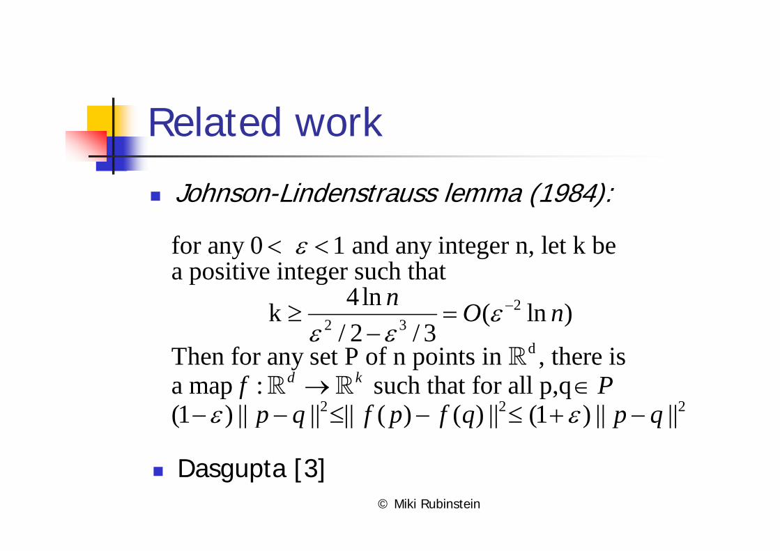
Johnson-Lindenstrauss lemma (1984):
22 3
d
for any 0 1 and any integer n, let k be a positive integer such that
4 ln k ( ln )/ 2 / 3
Then for any set P of n points in , there is a map : such that for all p,q(1
d k
n O n
f P
ε
εε ε
ε
−
< <
≥ =−
→ ∈− 2 2 2) || || || ( ) ( ) || (1 ) || ||p q f p f q p qε− ≤ − ≤ + −
Dasgupta [3]

© Miki Rubinstein
Johnson-Lindenstrauss Lemma
Any n point set in Euclidian space can be embedded in suitably high (logarithmic in n, independent of d) dimension without distorting the pairwise distances by more that a factor of )1( ε±

© Miki Rubinstein
Random mapping methodLet Let R be dxn matrix of random values where ||ri||=1 and each rij∈R is normally i.i.d with mean 0
[ 1] [ ] [ 1]
1
dx dxn nx
n
i ii
y R x d n
r x=
= <<
= ∑
nx ∈

© Miki Rubinstein
Random mapping method
1
21 2
1 0 00 1 0
0 0 1
n
n
xx
x x x x
x
⎛ ⎞⎛ ⎞ ⎛ ⎞ ⎛ ⎞⎜ ⎟⎜ ⎟ ⎜ ⎟ ⎜ ⎟⎜ ⎟⎜ ⎟ ⎜ ⎟ ⎜ ⎟+ + + = =⎜ ⎟⎜ ⎟ ⎜ ⎟ ⎜ ⎟⎜ ⎟⎜ ⎟ ⎜ ⎟ ⎜ ⎟
⎝ ⎠ ⎝ ⎠ ⎝ ⎠ ⎝ ⎠
11 12 1 1
21 22 2 21 2
1 2
n
nn
d d dn d
r r r yr r r y
x x x y
r r r y
⎛ ⎞ ⎛ ⎞ ⎛ ⎞ ⎛ ⎞⎜ ⎟ ⎜ ⎟ ⎜ ⎟ ⎜ ⎟⎜ ⎟ ⎜ ⎟ ⎜ ⎟ ⎜ ⎟+ + + = =⎜ ⎟ ⎜ ⎟ ⎜ ⎟ ⎜ ⎟⎜ ⎟ ⎜ ⎟ ⎜ ⎟ ⎜ ⎟⎝ ⎠ ⎝ ⎠ ⎝ ⎠ ⎝ ⎠

© Miki Rubinstein
Similarity
( , ) cos|| || || ||
if || || 1,|| || 1
then cos
u vsim u vu v
u v
u v
θ
θ
⋅= =
= =
= ⋅
© Miki Rubinstein
Random mapping methodHow will it affect the mutual similaritiesbetween the data vectors?As R is more orthonormal the better. however R is generally not orthogonalHecht-Nielsen [4]: in a high dimensional space, there exists a much larger number of almost orthogonal than orthogonal directionsSo, R might be sufficiently good approximation for a basis

© Miki Rubinstein
Transformation of similarities
Similarity measure:
Properties of ε:
( , ) cos for unit vectors|| || || ||
where ,
where for and 0
T T T n
T Tij i j ii
u vsim u v u vu v
x y n R Rm n m
R R I r r i j
θ
ε ε ε
⋅= = = ⋅
= ∈
= + = ≠ =
1 1( ) ( ) ( ) ( ) 0
d dT
ij i j ik jk ik jkk k
E E r r E r r E r E rε= =
⎛ ⎞ ⎡ ⎤= = = =⎜ ⎟ ⎣ ⎦⎝ ⎠∑ ∑

© Miki Rubinstein
Recall
Pearson correlation coefficient
Sample correlation
Geometric interpretation
,( , )
X YX Y
Cov X Yρσ σ
=
[ ], , 2 2
( )( )ˆ
( ) ( )
i ix y x y
i i
x x y yr
x x y yρ
− −= =
− −
∑∑ ∑
cos x yx x y y
θ ⋅=
⋅ ⋅

© Miki Rubinstein
RecallFisher (r2z) Transformation
Variance of z is estimate of the variance of the population correlation
Let X, Y normally distributedand let r be correlation of sample of size N from X,Y
1 1log2 1
then is approximately normally distributed with1standard deviation N-3
erzr
z
+=
−

© Miki Rubinstein
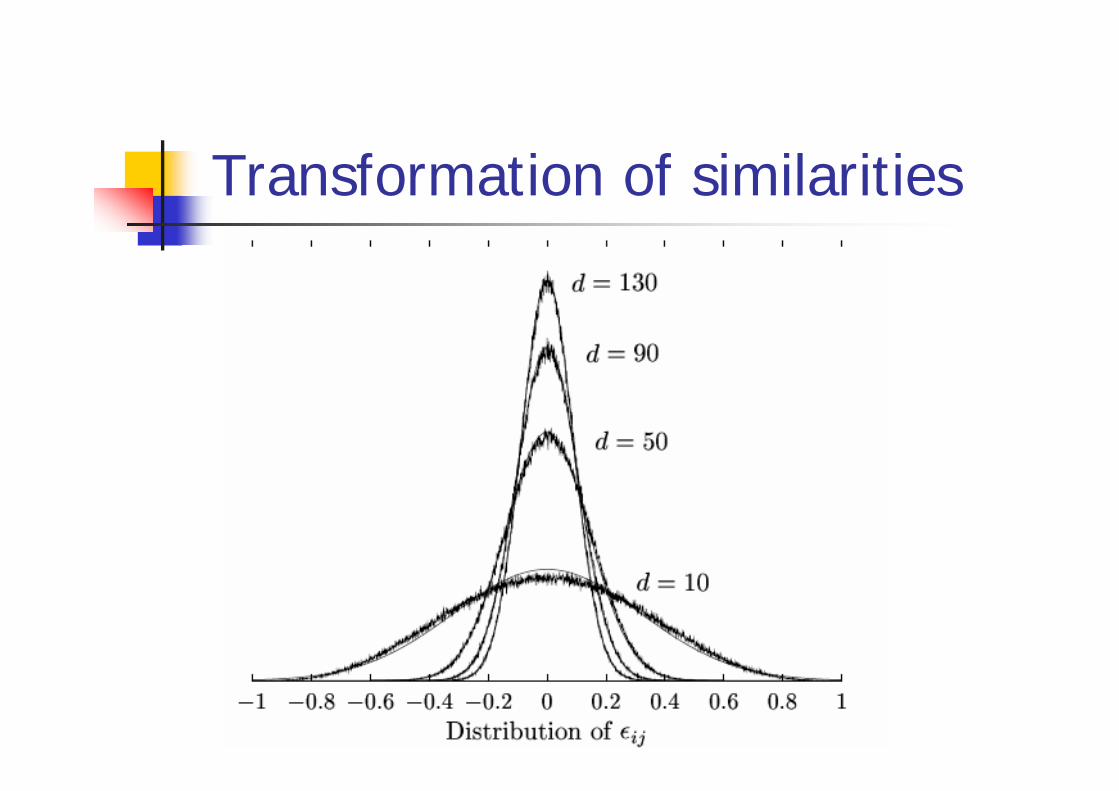
Transformation of similarities
Properties of ε:εij is an estimate of the correlation coefficient between two normally i.i.d random variables riand rj
2
11 ln is approximately normally distributed2 1
1with variance 1/ for large d-3
ij
ij
ddε
εε
σ
+
−
= ≈
as , Td R R I⇒ → ∞ →
© Miki Rubinstein
Transformation of similarities

© Miki Rubinstein
Transformation of similarities
Statistical propertiesLet , , and assume , are normalized
( ) = (recall 0)
let =
n
T T T T T T
Tkl k l kk
k l
kl k lk l
n m n m
x y n R Rm n I m n m n mn m n m e
n m
ε εε
δ ε
≠
≠
∈
= = + = ++ =∑
∑
( ) ( ) 0kl k l k l klk l k l
E E n m n m Eδ ε ε≠ ≠
⎛ ⎞= = =⎜ ⎟
⎝ ⎠∑ ∑

© Miki Rubinstein
Transformation of similaritiesVariance of δ:
2 2 2( ) ( ( )) [( )( )] 0
= [ ]
[ ]
[ ] 0 only for ( and ) or ( and )
kl k l pq p qk l p q
k l p q kl pqk l p q
kl pq ki li pj qj ki li pj qji j i j
kl pq
E E E n m n m
n m n m E
E E r r r r E r r r r
E k p l q k q l p
δσ δ δ ε ε
ε ε
ε ε
ε ε
≠ ≠
≠ ≠
= − = − =
⎡ ⎤ ⎡ ⎤= =⎢ ⎥ ⎢ ⎥
⎣ ⎦ ⎣ ⎦
≠ = = = =
∑ ∑∑∑
∑ ∑ ∑∑
1 2denote ( , ), ( , )c k p l q c k q l p= = = = = =

© Miki Rubinstein
Transformation of similaritiesVariance of δ:
2 2 2 2 21 2
2 2 2
2 2 2
(corresponds to , respectively)
=
= (1 ) ( || || 1,|| || 1)
= 1
k l k l l kk l k l
k l k k l lk l k k l k
k k k k l l k kk k l
k
n m n m n m c c
n m n m n m
n m n m n m n m n m
n
δ ε ε
ε
ε
σ σ σ
σ
σ
≠ ≠
≠ ≠
= +
⎡ ⎤+⎢ ⎥
⎣ ⎦⎡ ⎤⎛ ⎞
− + − = =⎢ ⎥⎜ ⎟⎝ ⎠⎣ ⎦
−
∑ ∑
∑ ∑ ∑ ∑
∑ ∑ ∑2 2 2 2 2 2
2 2 2 2
( )
= 1+( ) 2
k k k k kk k k
k k k kk k
m n m n m
n m n m
ε
ε
σ
σ
⎡ ⎤+ −⎢ ⎥
⎣ ⎦⎡ ⎤
−⎢ ⎥⎣ ⎦
∑ ∑ ∑
∑ ∑

© Miki Rubinstein
Transformation of similaritiesVariance of δ:
That is, the distortion of the inner products as aresult of applying random mapping is 0 on averageand its variance is proportional to the inverse ofthe dimensionality of the reduced space (x 2)
2
2 2
( ) 1 by Cauchy-Schwartz ( , normalized)
2 2 /
k kk
n m n m
dδ εσ σ
≤
⇒ ≤ ≈
∑

© Miki Rubinstein
Sparsity of the dataSay we constrain the input vectors to have L 1’s, and say K of those occur in same position in both vectors
( ) 1
2 2 2 2 2 2 22
2 2
Now, let's normalize , and we get K corresponding
dimenstions, each with value
=[1+( ) 2 ] [1 ( ) 2( )]
1 =[1 ( ) 2( ) ]
T
k k k kk k
K Kn mLL Ln m
LK Kn m n mL L
K KL L L
δ ε ε
ε
σ σ σ
σ
−
⇒ = =
⇒ − = + −
+ −
∑ ∑
Sparser data smaller variance of error!
© Miki Rubinstein
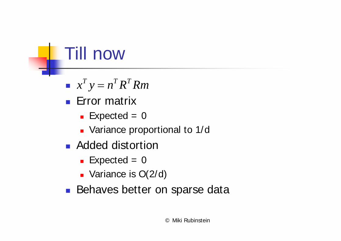
Till now
1Error matrix
Expected = 0Variance proportional to 1/d
Added distortionExpected = 0Variance is O(2/d)
Behaves better on sparse data
T T Tx y n R Rm=

© Miki Rubinstein
Self Organizing Maps

© Miki Rubinstein
Self Organizing Maps

© Miki Rubinstein
Self Organizing Maps
Kohonen Feature MapsUsually 1D or 2DEach map unit associated with an Rn
vectorUnsupervised, Single layer, Feed-Forward network

© Miki Rubinstein
SOM algorithmInitialization
RandomPattern
For each sample vector nFind winner, or BMU
Update rule:
Where hc(n),i is the neighborhood kernel and α(t) is the learning rate factor
( ),( 1) ( ) ( ) ( )[ ( )]i i c n i im t m t h t t n m tα+ = + −
( ) arg min{|| ||}ii
c n n m= −

© Miki Rubinstein
SOM visualization
wsom
© Miki Rubinstein
Back to Random Mapping
SOM should not be too sensitive to distortions by random mapping
Small neighborhoods in Rn will be mapped to small neighborhoods in Rd will probably be mapped to single MU or a set of close-by MUs

© Miki Rubinstein
WEBSOM document organizing system
Vector space model (Salton 1975)Vectors are histograms of words
i’th element indicates (function of) frequency of the i’th vocabulary term in the document
Direction of vector reflects doc context

© Miki Rubinstein
WEBSOM – example?
http://websom.hut.fi/websom/comp.ai.neural-nets-new/html/root.html
© Miki Rubinstein
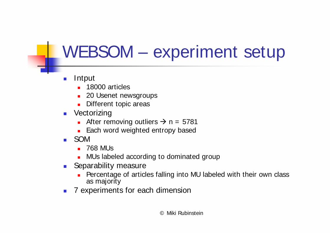
WEBSOM – experiment setupIntput
18000 articles20 Usenet newsgroupsDifferent topic areas
VectorizingAfter removing outliers n = 5781Each word weighted entropy based
SOM768 MUsMUs labeled according to dominated group
Separability measurePercentage of articles falling into MU labeled with their own class as majority
7 experiments for each dimension

© Miki Rubinstein
WEBSOM - results

© Miki Rubinstein
heuristicsDistance metric:
= expected norm of projection of unit vector to random subspace through the origin (JL scaling term)Image data
Constructing R:Set each entry of the matrix to an i.i.d. N(0,1) valueOrthogonalize the matrix using the Gram-Schmidt algorithmNormalize the columns of the matrix to unit length
1 2 1 2|| || / || ||x x n d Rx Rx− ⇒ −/n d

© Miki Rubinstein
heuristics
Achlioptas [2]:Simpler distributions that are JL compatible
Only 1/3 of the operations
1 with probability 1/63 0 with probability 2/3
1 with probability 1/6ijr
+⎧⎪= ⋅⎨⎪−⎩
1 with probability 1/2 1 with probability 1/2ijr +⎧= ⎨−⎩
© Miki Rubinstein
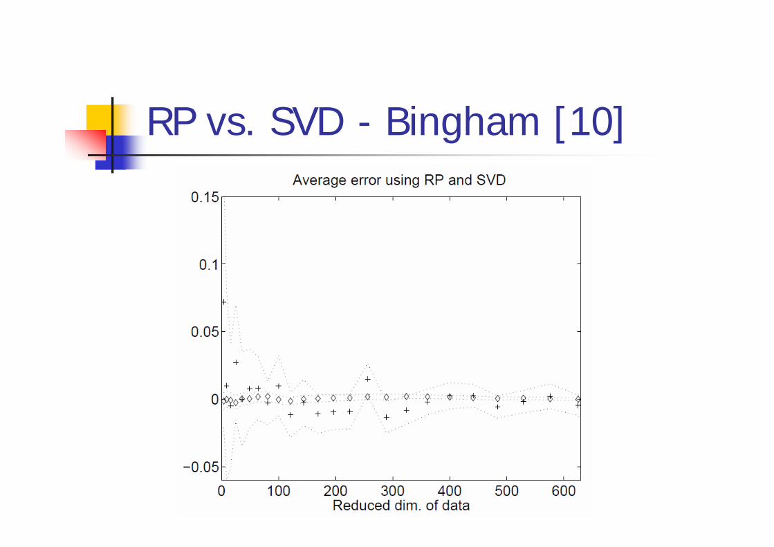
RP vs. SVD - Bingham [10]
n = 50002262 newsgroup documentsRandomly chosen pairs of data vectors u, vError = uv – (Ru)(Rv)95% confidence intervals over 100 pairs of (u,v)
© Miki Rubinstein
RP vs. SVD - Bingham [10]

© Miki Rubinstein
RP on Mixture of Gaussians
data from a mixture of k Gaussians can be projected into O(logk) dimensions while still retaining the approximate level of separation between the clusters
Projected dimension independent of number of points and original dimensionEmpirically shown for 10lnkDecision of reduced dimension is highly studied
Dasgupta [9] – for further details!

© Miki Rubinstein
RP on Mixture of Gaussians
The dimension is drastically reduced while eccentric clusters remain well separated and become more spherical

© Miki Rubinstein
RP ensembles – Fern [7]
Experience of distorted, unstable clustering performanceDifferent runs may uncover different parts of the structure in the data that complement one another

© Miki Rubinstein
RP ensemblesMultiple runs of RP + EM:
Project to lower subspace dUse EM to generate a probabilistic model of a mixture of k Gaussians
Average the Pijs across n runsGenerate final clusters based on P
Can iterate of different (reduced) subspacesFern [7] - for more details!
1( | , ) ( | , )
k
ijl
P P l i P l jθ θ θ=
= ∑

© Miki Rubinstein
Face recognition with RP –Goal [11]
Training set: M NxN vectors (each represents a face)
Algorithm:1. compute average face:
2. Subtract mean face from each face:
3. Generate random operator R4. Project normalized faces to random subspace:
1
1 M
iiM =
Ψ = Γ∑
i iΦ = Γ − Ψ
i iw R= Φ

© Miki Rubinstein
Face recognition with RP
Recognition:1. Normalize2. Project to same random space3. Compare projection to database

© Miki Rubinstein
Face recognition with RP
Face representations need not be updated when face database changesUsing ensembles of RPs seems promisingGoel [11] – for more details!

© Miki Rubinstein
Face recognition with RP –example results

© Miki Rubinstein
ConclusionsComputationally much simpler
k data vectors, d << NRP: O(dN) to build, O(dkN) to apply
If R has c nonzero entries: O(ckN) to applyPCA: O(kN2)+O(N3)
Independent of the dataHas been applied on various problems and shown satisfactory results:
Information retrievalMachine learningImage/text analysis

© Miki Rubinstein
Conclusions
Computation vs. PerformanceBad results?Applying Johnson-Lindenstrauss on Kaski’s setup yields k~2000 (?)

© Miki Rubinstein
?
Sanjoy Dasgupta

© Miki Rubinstein
References[1] S. Kaski. Dimensionality reduction by random mapping. In Proc. Int. Joint Conf. on Neural Networks, volume 1, pages 413–418, 1998.[2] D. Achlioptas. Database-friendly random projections. In Proc. ACM Symp. on the Principles of Database Systems, pages 274–281, 2001.[3] S. Dasgupta and A. Gupta. An elementary proof of the Johnson-Lindenstrauss lemma. Technical Report TR-99-006, International Computer Science Institute, Berkeley, California, USA, 1999.[4] R. Hecht-Nielsen. Context vectors: general purpose approximate meaning representations self-organized from raw data. In J.M. Zurada, R.J. Marks II, and C.J. Robinson, editors, Computational Intelligence: Imitating Life, pages 43–56. IEEE Press, 1994.[5] P. Indyk and R. Motwani. Approximate nearest neighbors: Towards removing the curse of dimensionality. In Proc. of 30th STOC, 1998 [6] D. Fradkin and D. Madigan. Experiments with random projections for machine learning. In KDD '03: Proceedings of the ninth ACM SIGKDD international conference on Knowledge discovery and data mining, pages 517--522, 2003

© Miki Rubinstein
References[7] Xiaoli Z. Fern and Carla E. Brodley, "Cluster ensembles for high dimensional data clustering: An empirical study", Techenical report CS06-30-02[8] C.H. Papadimitriou, P. Raghvan, H. Tamaki and S. Vempala, “Latent semantic analysis: A probabilistic analysis,” in Proceedings of 17th ACM Symp. On the principles of Database Systems, pp. 159–168, 1998.[9] Sanjoy Dasgupta, Experiments with Random Projection, Proceedings of the 16th Conference on Uncertainty in Artificial Intelligence, p.143-151, June 30-July 03, 2000[10] E. Bingham and H. Mannila, “Random projection in dimensionality reduction: applications to image and text data,” in Proceedings of the 7th ACM SIGKDD International Conference on Knowledge Discovery and Data Mining, pp. 245–250, 2001[11] N. Goel, G. Bebis, and A. Nefian. Face recognition experiments with random projection. In Proceedings SPIE Vol. 5779, pages 426--437, 2005

© Miki Rubinstein
ReferencesSantosh S. Vempala (2004)The Random Projection Method