Reduction of Fan Generated Tonal Noise in a Ventilation...

Reduction of Fan Generated Tonal Noise in a Ventilation Duct with Applications to theInternational Space Station

Holly SmithWorkforce Development Grant

Arkansas Space Grant Consortium

Johnson Space Center Acoustics O!ceHabitability and Environmental Factors Branch

Space and Life Sciences DirectorateMentor: Christopher Allen

Abstract

The ventilation system aboard the International Space Station (ISS) is a cruciallife-support system that provides the crew with circulated, filtered air; however, thissystem contains fans that generate unwanted tonal noise. The tonal noise producedby the fans may interfere with the daily activities of the crew as well as pose a po-tential health hazard. Because a Helmholtz resonator’s unique geometry allows it toresonate at a specific frequency, it is possible to design a Helmholtz resonator that willeliminate the single frequency tonal noise when adjacently attached to a ventilationduct. Therefore, this project focused on how to incorporate Helmholtz resonators intoa model ventilation duct in order to eliminate tonal noise produced by a fan.

This project was completed using two di!erent methods: analytical and experi-mental. The analytical approach involved calculating transmission loss predictions inorder to determine how various Helmholtz resonators would a!ect the sound level of thetonal noise when introduced into the ventilation duct. The experimental approach in-volved constructing a model ventilation duct from medium density fiberboard (MDF).Multiple, adjustable Helmholtz resonators constructed from PVC and MDF were intro-duced adjacently to the duct, and measurements of the Helmholtz resonators’ e!ectson the sound level were obtained. These measurements are compared to the numericalpredictions calculated during the analytical stage.

2

Contents

1 Theory 41.1 International Space Station Acoustic Requirements . . . . . . . . . . . . . . 41.2 Fan Generated Tonal Noise . . . . . . . . . . . . . . . . . . . . . . . . . . . 51.3 Helmholtz Resonators . . . . . . . . . . . . . . . . . . . . . . . . . . . . . . 51.4 Transmission Loss . . . . . . . . . . . . . . . . . . . . . . . . . . . . . . . . . 7

1.4.1 Transmission Loss Prediction - Helmholtz Resonator with No Ther-moviscous losses . . . . . . . . . . . . . . . . . . . . . . . . . . . . . . 9

1.4.2 Transmission Loss Prediction - Cavity and Neck Impedance . . . . . 9

2 Emperical Predictions 102.1 Fan Generated Tonal Noise Prediction . . . . . . . . . . . . . . . . . . . . . 102.2 Pressure Antinode Prediction . . . . . . . . . . . . . . . . . . . . . . . . . . 112.3 Transmission Loss Prediction . . . . . . . . . . . . . . . . . . . . . . . . . . 11

3 Experimental Procedure and Results 143.1 The Experimental Duct . . . . . . . . . . . . . . . . . . . . . . . . . . . . . 143.2 Fan Generated Tonal Noise Measurement . . . . . . . . . . . . . . . . . . . . 163.3 Adjustable Helmholtz Resonators . . . . . . . . . . . . . . . . . . . . . . . . 183.4 Insertion Loss . . . . . . . . . . . . . . . . . . . . . . . . . . . . . . . . . . . 22

4 Conclusion 234.1 Project Conclusions . . . . . . . . . . . . . . . . . . . . . . . . . . . . . . . . 234.2 Future Experiments . . . . . . . . . . . . . . . . . . . . . . . . . . . . . . . . 264.3 Acknowledgements . . . . . . . . . . . . . . . . . . . . . . . . . . . . . . . . 26

Appendix A:Determining the Fan Speed of a 4184/2XH ebmpapst 4100N Series Tubeax-ial Fan 28

Appendix B:Sample Mathematica File for Determining Transmission Loss - First Pre-diction Method 30

Appendix C:Sample Mathematica File for Determining Transmission Loss - SecondPrediction Method 32

3

1 Theory

1.1 International Space Station Acoustic Requirements

The Crew Quarters (CQ) aboard the International Space Station (ISS) contains a venti-

lation system composed of a duct with two fans. The supply fan introduces filtered air into

the CQ whereas the return fan removes the air from the CQ and back into the ventilation

system. Due to the nature of axial fans, both fans are responsible for creating tonal noise

that may a"ect the health and performance of the ISS crew. Therefore, it is imperative to

eliminate any tonal noise that violates the currently existing acoustic safety standards.

The acoustic sound levels of the generated tonal noise must meet three basic criteria: (1)

the sound levels must not pose a health hazard to the crew; (2) the sound levels should not

a"ect crew performance; and (3) the sound levels should support a habitable and comfortable

living and work environment.[1] Because the fans can operate at low, medium, and high

settings1, there are di"erent noise criterion curves for the di"erent settings. Currently, the

fans are considered to produce continuous noise when operated at the low setting2. The

maximum noise criteria curve for continuous noise in the CQ during sleeping hours is NC-

40.[2] The noise produced by the fans in either the medium or high setting is considered to be

intermittent noise3. The acceptable noise criterion curve for intermittent noise is NC-37.[2]

For the sake of simplicity, this investigation focuses on limiting to the tonal noise produced

by the return fan at its highest setting (24 Volts) to the NC-40 curve4.

Along with the continuous and intermittent noise criteria, tonal noise must meet the

sound pressure level specified by the Narrow-Band Annoyance criteria. According to this

requirement, a single frequency tone must be ten decibels less than the broadband sound

1For this investigation, the fan speeds at the low, medium, and high settings were considered to beapproximately 2000, 3300, and 4030 rotations per minute for the supply fan and 2567, 3667, and 4400 rpmfor the return fan. These fan speeds are based on an approximation that is explained in Appendix A.

2This study assumes that the fans are operated at the low setting during the crew’s sleep periods.[2]3This study assumes that the duration of these settings does not exceed eight hours.4Because multiple sound sources have sound pressure levels that logarithmically add to produce an overall

sound pressure level, this fan must actually match the NC-34 curve.

4

pressure level of its octave band.[3] If tonal noise created by ventilation fans is higher than

the accepted sound pressure level set by these criteria, then these ventilation systems may

pose serious hazards to the health and safety of the crew. This project aims to minimize the

amount of tonal noise produced by fans located in ventilation ductwork by investigating the

incorporation of Helmholtz resonators as side-branches to the duct.

1.2 Fan Generated Tonal Noise

Tonal noise in ventilation ducts often occurs as a result of an operating fan within the

duct. This tonal noise is produced by a periodic distubance of the fan’s inflow or the

interaction of the downstream flow with a stationary object.[4] If the noise occurs as a result

of the fan’s inflow, then the tonal noise can be predicted by the equation:

!n =nKN

60, n=1,2,3,... (1)

In this equation, !n is the nth-harmonic frequency, n is an integer number, K is the number

of fan blades, and N is the speed of the fan in revolutions per minute.[5]

1.3 Helmholtz Resonators

A Helmholtz resonator consists of a hollow neck attached to an empty volume. The

behavior of the air within the flask is comparable to a driven, damped spring-mass system as

shown in Figure 1. When a sinusoidal force acts upon the air within the flask, the air within

the neck is comparable to a mass oscillating on a spring. The air within the cavity serves

as the “spring” and is responsible for providing the system’s sti"ness element. Due to its

contact with the neck’s wall, the mass of air within the neck will experience thermoviscous

losses, and this friction will cause a portion of the acoustic energy to be converted into heat.

5

Figure 1: Motion of air

within a Helmholtz res-

onator.

Like a driven, damped spring-mass system, the Helmholtz res-

onator will resonate or produce sound when driven at its natural

frequency. The resonator’s natural frequency is determined by its

dimensions and the speed of sound and is described by the equation:

!o =c

2"

!Sn

L!V(2)

In this equation, !o is the natural frequency, c is the speed of sound

in air, Sn is the the cross-sectional area of the neck, L! is the e"ective

length of the neck,5 and V is the volume.[6] The production of

sound that occurs at resonance will lead to more energy loss due to

radiation resistance at the opening.

Helmholtz resonators can be incorporated into ventilation ducts as side branches in order

to reduce the tonal noise generated by fans within the duct. The amount of tonal noise

reduction can be described by the power transmission coe!cient, T!, which describes how

much acoustic power is transmitted through the duct. The power transmission coe!cient

for this type of band-stop filter is given by:

T! =1

1 +"

c/2Sd

!L!/Sn"c2/!V

#2 (3)

Here, Sd represents the cross-sectional area of the duct in which the Helmholtz resonator is

being incorporated. When T! = 0, none of the incoming acoustic power is transmitted into

the duct. Instead, the incoming acoustic energy enters the resonator and is reflected back

towards the source, causing destructive interference. Solving Equation 4 for T! = 0 yields

the resonance frequency of the Helmholtz resonator.[6] Therefore, by designing a Helmholtz

resonator to resonate at the frequency of the tonal noise, the resonator can cause near tonal

5The e!ective length is related to the length of the neck by the equation: L! = L + 1.4a, where a is theradius of the neck’s opening. The e!ective length accounts for the shape of the opening of the resonator.The openings for the Helmholtz resonators used in this experiment are unflanged.

6

reflection of acoustic waves with frequencies near that of the resonance frequency.

1.4 Transmission Loss

Figure 2: A cylindrical Helmholtz resonator attached to a duct as a side-branch. Thedimensions of the Helmholtz resonator include a volume of cross-sectional area Scavity, heighth, neck of cross-sectional area Sneck, and length L. The duct has a cross-sectional area ofSduct. A represents the acoustic wave originating from a source, and B and C are the reflectedand transmitted waves, respectively.

Figure 2 shows a duct with a Helmholtz resonator adjacently as a side-branch. The

pressures and velocities at points 1 and 2 along the duct are related by the transfer matrix

for a Helmholtz resonator:

$

%&p1

#S1u1

'

() =

$

%&1 0

1Zr

1

'

()

$

%&p2

#S2u2

'

() (4)

In this equation pn is the pressure at a point within the duct, # is the air density, Sn is

the cross-sectional area of the duct, un is the velocity, and Zr is the Helmholtz resonator’s

acoustic impedance6.[4] A common measurement of a Helmholtz resonator’s e"ectiveness

6Acoustic impedance is defined as pressure divided by volume velocity or Z = p/U . Acoustic impedancecan also be defined as Z = !c

S where S is the cross-sectional area of the acoustic device in question. It iscomposed of both real and imaginary parts: Z = R + jX , where R is the acoustic resistance and X is theacoustic reactance. For a Helmholtz resonator, Z = (Rr + Rw) + j(!m ! s!), where Rr is the radiationresistance, Rw is the thermoviscous resistance, m is the mass of air in the neck (m = "0SL!), s is the sti!nessof air in the volume (s = !0c2S2

V ), and ! is the angular resonance frequency.

7

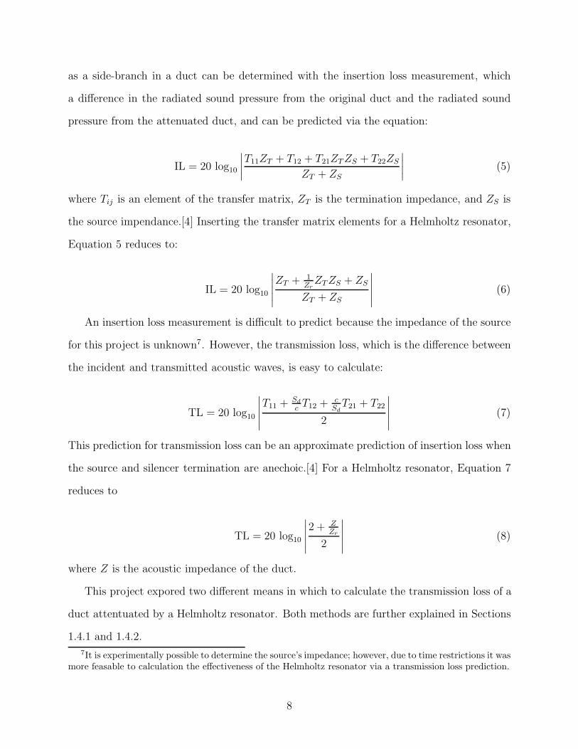
as a side-branch in a duct can be determined with the insertion loss measurement, which

a di"erence in the radiated sound pressure from the original duct and the radiated sound

pressure from the attenuated duct, and can be predicted via the equation:

IL = 20 log10

****T11ZT + T12 + T21ZT ZS + T22ZS

ZT + ZS

**** (5)

where Tij is an element of the transfer matrix, ZT is the termination impedance, and ZS is

the source impendance.[4] Inserting the transfer matrix elements for a Helmholtz resonator,

Equation 5 reduces to:

IL = 20 log10

*****ZT + 1

ZrZT ZS + ZS

ZT + ZS

***** (6)

An insertion loss measurement is di!cult to predict because the impedance of the source

for this project is unknown7. However, the transmission loss, which is the di"erence between

the incident and transmitted acoustic waves, is easy to calculate:

TL = 20 log10

*****T11 + Sd

c T12 + cSd

T21 + T22

2

***** (7)

This prediction for transmission loss can be an approximate prediction of insertion loss when

the source and silencer termination are anechoic.[4] For a Helmholtz resonator, Equation 7

reduces to

TL = 20 log10

*****2 + Z

Zr

2

***** (8)

where Z is the acoustic impedance of the duct.

This project expored two di"erent means in which to calculate the transmission loss of a

duct attentuated by a Helmholtz resonator. Both methods are further explained in Sections

1.4.1 and 1.4.2.7It is experimentally possible to determine the source’s impedance; however, due to time restrictions it was

more feasable to calculation the e!ectiveness of the Helmholtz resonator via a transmission loss prediction.

8

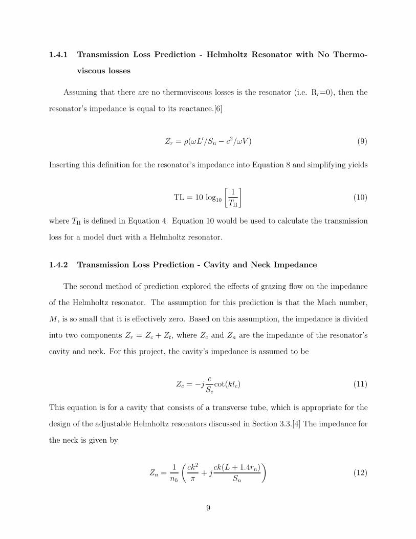
1.4.1 Transmission Loss Prediction - Helmholtz Resonator with No Thermo-

viscous losses

Assuming that there are no thermoviscous losses is the resonator (i.e. Rr=0), then the

resonator’s impedance is equal to its reactance.[6]

Zr = #($L!/Sn ! c2/$V ) (9)

Inserting this definition for the resonator’s impedance into Equation 8 and simplifying yields

TL = 10 log10

+1

T!

,(10)

where T! is defined in Equation 4. Equation 10 would be used to calculate the transmission

loss for a model duct with a Helmholtz resonator.

1.4.2 Transmission Loss Prediction - Cavity and Neck Impedance

The second method of prediction explored the e"ects of grazing flow on the impedance

of the Helmholtz resonator. The assumption for this prediction is that the Mach number,

M , is so small that it is e"ectively zero. Based on this assumption, the impedance is divided

into two components Zr = Zc + Zt, where Zc and Zn are the impedance of the resonator’s

cavity and neck. For this project, the cavity’s impedance is assumed to be

Zc = !jc

Sccot(klc) (11)

This equation is for a cavity that consists of a transverse tube, which is appropriate for the

design of the adjustable Helmholtz resonators discussed in Section 3.3.[4] The impedance for

the neck is given by

Zn =1

nh

-ck2

"+ j

ck(L + 1.4rn)

Sn

.(12)

9

where nh is the number of necks and rn is the neck’s radius8.[4] Adding Equations 11 and

12 yield the acoustic impedance of the resonator, and this value is inserted into Equation 8

to yield:

TL = 20 log10

********

2 +!0cSd

"j cSc

cot(klc)+ 1nh

“ck2

" +j ck(L+1.4rn)Sn

”

2

********(13)

2 Emperical Predictions

2.1 Fan Generated Tonal Noise Prediction

Due to time limitations, the goal of this project was to show successful attentuation

of the 366 Hz tone produced by the fan operating at 24 Volts by adjacently inserting a

Helmholtz resonator into the duct. Prior to conducting the insertion loss experiment, it

was necessary to predict the frequency values of the tonal noise and the e"ectiveness of a

Helmholtz resonator designed to eliminate a specific tonal noise produced by a fan within a

ventilation duct. These values would later be compared to experimental measurements.

The following frequency predictions for the fan were predicted using Equation 1 and the

estimated fan speeds given in Table 4 for 12, 18, and 22 V (supply fan) supplied to the fan

as well as 14, 20, and 24 V (return fan).

Volts Fan 1st 2nd 3rd 4th 5th

Supplied Speed Harmonic Harmonic Harmonic Harmonic Harmonicto Fan (rpm) (Hz) (Hz) (Hz) (Hz) (Hz)

12 2200 183 367 550 733 91718 3300 275 550 825 1100 137522 4033 336 672 1008 1344 1681

Table 1: The first five harmonic frequencies for the low, medium, and high settings of thesupply fan.

8This equation di!ers from Beranek and Ver’s in that the correction for the neck, L + 1.4rn, is for anunflanged neck. Beranek nd Ver assume a flanged neck.

10

Volts Fan 1st 2nd 3rd 4th 5th

Supplied Speed Harmonic Harmonic Harmonic Harmonic Harmonicto Fan (rpm) (Hz) (Hz) (Hz) (Hz) (Hz)

14 2567 214 428 642 856 106920 3667 306 611 917 1222 152824 4400 367 733 1100 1467 1833

Table 2: The first five harmonic frequencies for the low, medium, and high settings of thereturn fan. The frequencies listed in the third row would be compared to the measured tonalfrequencies recorded during the experimental stage of the project. These results can be seenin Section 3.2.

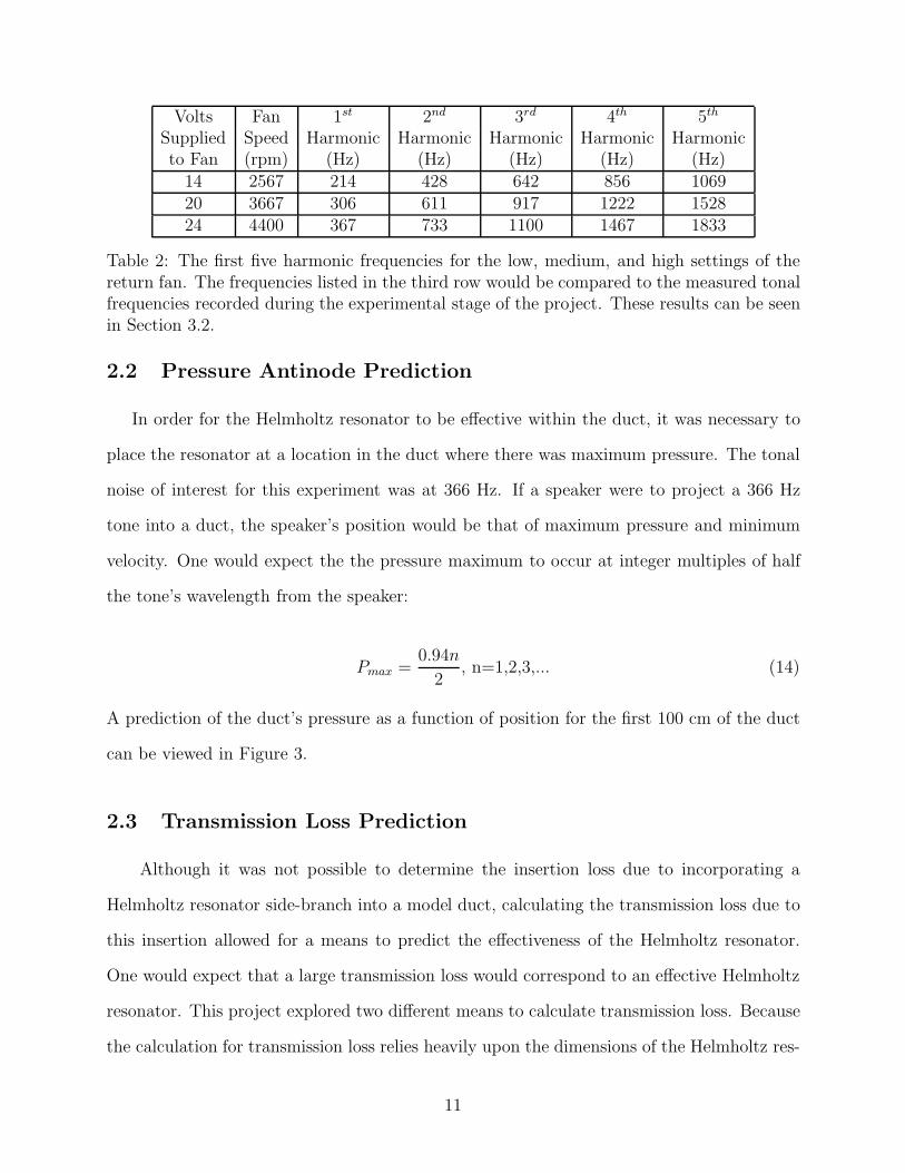
2.2 Pressure Antinode Prediction

In order for the Helmholtz resonator to be e"ective within the duct, it was necessary to

place the resonator at a location in the duct where there was maximum pressure. The tonal

noise of interest for this experiment was at 366 Hz. If a speaker were to project a 366 Hz

tone into a duct, the speaker’s position would be that of maximum pressure and minimum

velocity. One would expect the the pressure maximum to occur at integer multiples of half

the tone’s wavelength from the speaker:

Pmax =0.94n

2, n=1,2,3,... (14)

A prediction of the duct’s pressure as a function of position for the first 100 cm of the duct

can be viewed in Figure 3.

2.3 Transmission Loss Prediction

Although it was not possible to determine the insertion loss due to incorporating a

Helmholtz resonator side-branch into a model duct, calculating the transmission loss due to

this insertion allowed for a means to predict the e"ectiveness of the Helmholtz resonator.

One would expect that a large transmission loss would correspond to an e"ective Helmholtz

resonator. This project explored two di"erent means to calculate transmission loss. Because

the calculation for transmission loss relies heavily upon the dimensions of the Helmholtz res-

11

0

0.2

0.4

0.6

0.8

1

0 20 40 60 80 100

P/P m

ax

Distance from Speaker (cm)

Predicted Pressure in a Driven Duct

Figure 3: At x=0 (the theoretical position of the speaker), there exists a pressure maxi-mum. For a 366 Hz tone, the next pressure maximum is located half a wavelength away orapproximately 46.86 cm.

onator, the goal of each prediction was to optimize the dimensions for greatest transmission

loss. Therefore, Mathematica notebooks were created in order to simplify the prediction

process by calculating the transmission loss for given dimensions over a range of frequencies.

Both notebooks were adjustable, which allowed for various dimensions (in SI Units) to be

tested. Once the notebook completes the calculation, it generates a text file that can later

be used to generate tranmission loss graphs. A sample Mathematica notebook can be viewed

in Appendix B.

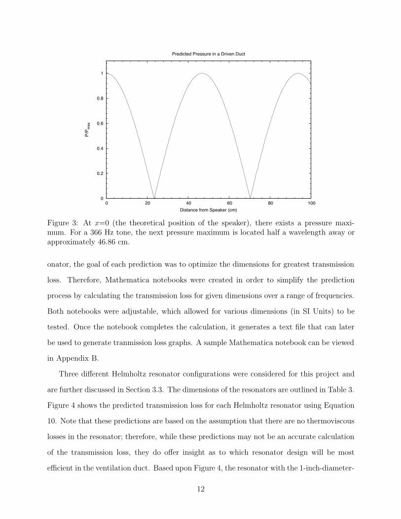
Three di"erent Helmholtz resonator configurations were considered for this project and

are further discussed in Section 3.3. The dimensions of the resonators are outlined in Table 3.

Figure 4 shows the predicted transmission loss for each Helmholtz resonator using Equation

10. Note that these predictions are based on the assumption that there are no thermoviscous

losses in the resonator; therefore, while these predictions may not be an accurate calculation

of the transmission loss, they do o"er insight as to which resonator design will be most

e!cient in the ventilation duct. Based upon Figure 4, the resonator with the 1-inch-diameter-

12

neck Helmholtz resonator was predicted to be the most e!cient at reducing the 366 Hz tone

produced by the ventilation fan operating at 24 V.

Neck Neck Volume Volume ResonanceDiameter (in) Length (in) Diameter (in) Height (in) Frequency (Hz)

0.50 0.5 3 1.125 366.30.75 0.5 3 2.1 366.21 0.5 3 3.1875 366.3

Table 3: Each row corresponds to the dimensions of a Helmholtz resonator. Each resonatorwas identified by the diameter of its neck. Note that the dimensions are given in standardunits (i.e. inches). Dimensions in standard units were necessary for construction purposesand would later be converted into SI units for calculations.

0

5

10

15

20

25

30

35

350 355 360 365 370 375 380

Tran

smiss

ion

Loss

(dB)

Frequency/Frequencymax

Transmission Loss Predictions for Various Helmholtz Resonators

1/2-Inch-Diameter Neck3/4-Inch-Diameter Neck

1-Inch-Diameter Neck

Figure 4: The transmission loss predictions for three Helmholtz resonators of varying size.The dimensions of each resonator is outlined in Table 3. The ’bump’ located on the left ofthe three resonance curves is probably a result of the Mathematica program not iterating insmall enough increments.

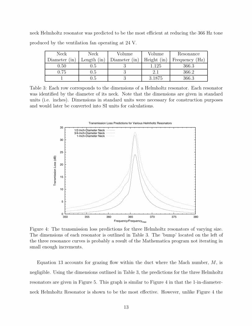
Equation 13 accounts for grazing flow within the duct where the Mach number, M , is

negligible. Using the dimensions outlined in Table 3, the predictions for the three Helmholtz

resonators are given in Figure 5. This graph is similar to Figure 4 in that the 1-in-diameter-

neck Helmholtz Resonator is shown to be the most e"ective. However, unlike Figure 4 the

13

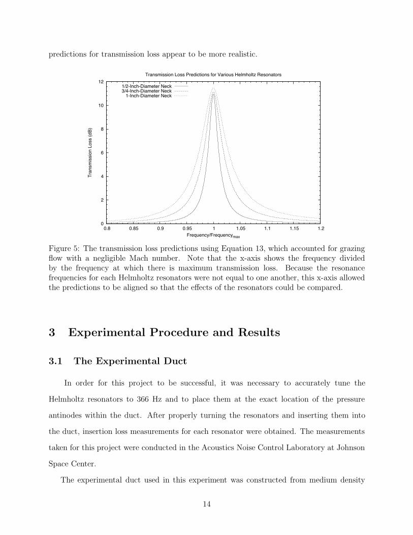
predictions for transmission loss appear to be more realistic.

0

2

4

6

8

10

12

0.8 0.85 0.9 0.95 1 1.05 1.1 1.15 1.2

Tran

smiss

ion

Loss

(dB)

Frequency/Frequencymax

Transmission Loss Predictions for Various Helmholtz Resonators


1-Inch-Diameter Neck

Figure 5: The transmission loss predictions using Equation 13, which accounted for grazingflow with a negligible Mach number. Note that the x-axis shows the frequency dividedby the frequency at which there is maximum transmission loss. Because the resonancefrequencies for each Helmholtz resonators were not equal to one another, this x-axis allowedthe predictions to be aligned so that the e"ects of the resonators could be compared.

3 Experimental Procedure and Results

3.1 The Experimental Duct

In order for this project to be successful, it was necessary to accurately tune the

Helmholtz resonators to 366 Hz and to place them at the exact location of the pressure

antinodes within the duct. After properly turning the resonators and inserting them into

the duct, insertion loss measurements for each resonator were obtained. The measurements

taken for this project were conducted in the Acoustics Noise Control Laboratory at Johnson

Space Center.

The experimental duct used in this experiment was constructed from medium density

14

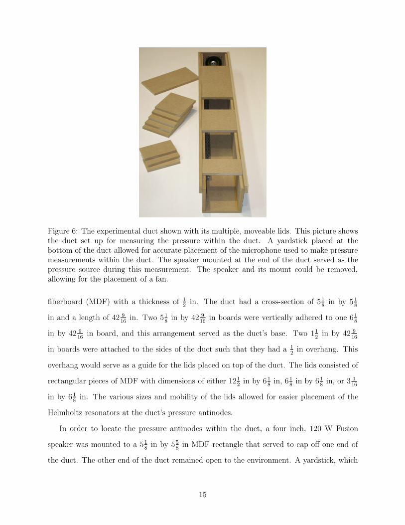
Figure 6: The experimental duct shown with its multiple, moveable lids. This picture showsthe duct set up for measuring the pressure within the duct. A yardstick placed at thebottom of the duct allowed for accurate placement of the microphone used to make pressuremeasurements within the duct. The speaker mounted at the end of the duct served as thepressure source during this measurement. The speaker and its mount could be removed,allowing for the placement of a fan.

fiberboard (MDF) with a thickness of 12 in. The duct had a cross-section of 51

8 in by 518

in and a length of 42 916 in. Two 51

8 in by 42 916 in boards were vertically adhered to one 61

8

in by 42 916 in board, and this arrangement served as the duct’s base. Two 11

2 in by 42 916

in boards were attached to the sides of the duct such that they had a 12 in overhang. This

overhang would serve as a guide for the lids placed on top of the duct. The lids consisted of

rectangular pieces of MDF with dimensions of either 1212 in by 61

8 in, 618 in by 61

8 in, or 3 116

in by 618 in. The various sizes and mobility of the lids allowed for easier placement of the

Helmholtz resonators at the duct’s pressure antinodes.

In order to locate the pressure antinodes within the duct, a four inch, 120 W Fusion

speaker was mounted to a 518 in by 55

8 in MDF rectangle that served to cap o" one end of

the duct. The other end of the duct remained open to the environment. A yardstick, which

15

0

0.2

0.4

0.6

0.8

1

0 20 40 60 80 100

Pres

sure

/Pre

ssur

e max

Distance from Speaker (cm)

Pressure Versus Distance from Speaker in Duct

Experimental DataPredicted

Figure 7: The horizontal di"erence between the experimental data and the predicted pressurecurve may arise from the fact that 0 cm corresponded to the speaker’s mount and not to thelocation at which the speaker was emitting maximum pressure.

was placed at the bottom of the duct, lied flush against the mount. A Larson-Davis Model

2541 12-in free-field microphone was placed in numerous locations within the duct while the

speaker emitted a 366 Hz tone. The results of this pressure measurement can be viewed in

Figure 7.

3.2 Fan Generated Tonal Noise Measurement

Figures 8(a) and 8(b) show the fan used in this experiment and its dimensions. In

order to determine the tonal noise frequencies of the fan, it was inserted at one end of the

experimental duct shown in Figure 6 and was operated at the high setting for the return fan-

24 Volts. A Larson Davis Model 2541 12 in free-field microphone was placed approximately a

foot away from the opening of the duct and was protected with a windscreen. A narrowband,

800 line measurement of the tonal noise within a 0 to 2500 Hz range was recorded by a Larson

Davis 2900B analyzer. The narrowband tonal noise measurement shown in Figure 9 is an

16

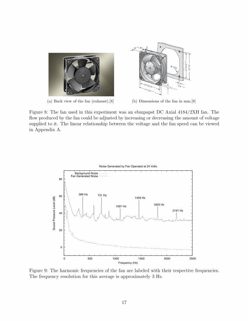
(a) Back view of the fan (exhaust).[8] (b) Dimensions of the fan in mm.[8]

Figure 8: The fan used in this experiment was an ebmpapst DC Axial 4184/2XH fan. Theflow produced by the fan could be adjusted by increasing or decreasing the amount of voltagesupplied to it. The linear relationship between the voltage and the fan speed can be viewedin Appendix A.

0

20

40

60

80

0 500 1000 1500 2000 2500

Soun

d Pr

essu

re L

evel

(dB)

Frequency (Hz)

Noise Generated by Fan Operated at 24 Volts

366 Hz 731 Hz

1097 Hz

1459 Hz

1825 Hz

2191 Hz

Background NoiseFan Generated Noise

Figure 9: The harmonic frequencies of the fan are labeled with their respective frequencies.The frequency resolution for this average is approximately 3 Hz.

17

average of five tonal noise measurements that were each averaged over twenty seconds9. The

tonal peaks labeled with their frequencies correspond to the predicted tonal noise values for

the fan. The first five harmonic frequencies are listed in Table 2.

3.3 Adjustable Helmholtz Resonators

Figure 10: The two Helmholtz resonators pictured here have neck diameters of 12 in and 3

4 in.The plunger on the far right was equipped with a Bruel & Kjaer Type 4138 1

4 -in microphonethat served as a tool for accurate tuning of the resonator.

The Helmholtz resonators used in this experiment were constructed of MDF and

PVC pipe. Two of the resonators (12- and 3

4-inch-diameters) were constructed for a prior

experiment. The necks of both resonators were created by cutting the appropriate diameter

holes into the center of a 618 in by 61

8 in duct lid. Three-inch-diameter PVC pipes with lengths

of 14 in were adhered to the lid using epoxy. Black plungers, which had a length of 112 in and

a diameter of approximately 3 in when lined with white foam, were then inserted into the

three-inch-inner-diameter PVC pipes. The mobility of the plungers within the pipe allowed

the volume of this resonator’s cavity to be easily changed, therefore allowing the resonator

to be tuned to multiple frequencies10. Another Helmholtz resonator with a 1-inch-diameter

9Unless otherwise noted, each graph containing SPL narrowband measurements were evaluated at thesame settings.

10The frequency range for which these resonators could be tuned was limited. Assuming that the cavity

18

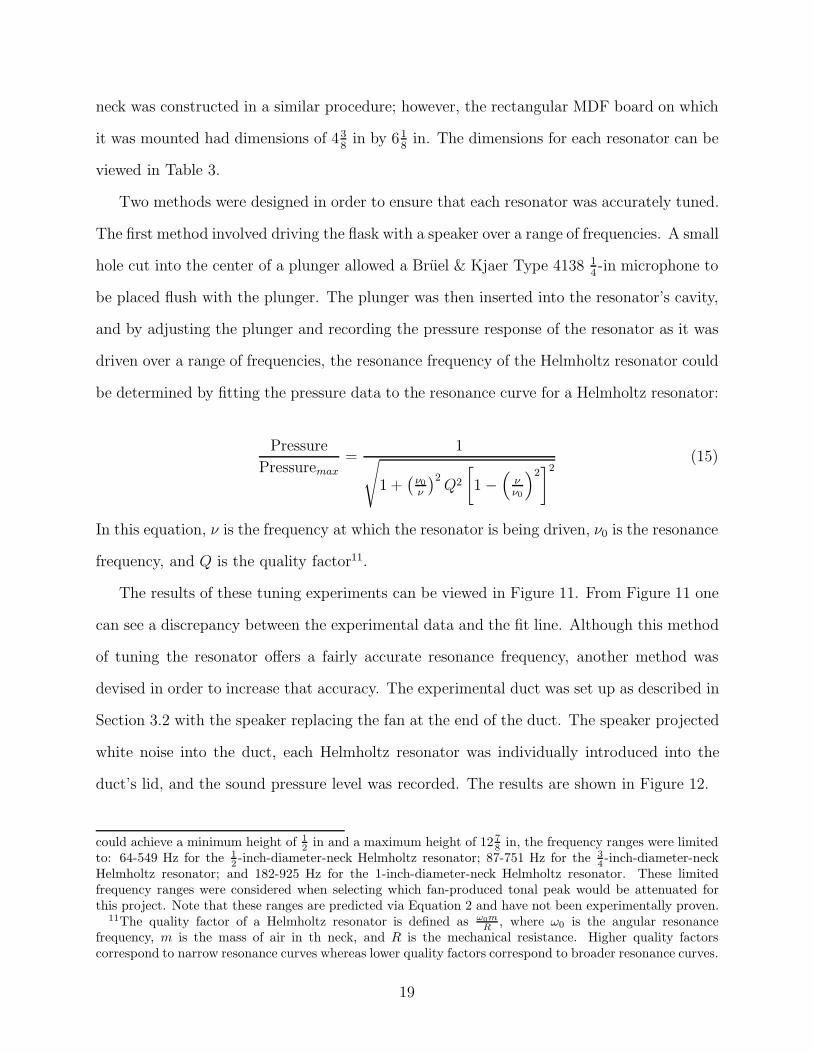
neck was constructed in a similar procedure; however, the rectangular MDF board on which

it was mounted had dimensions of 438 in by 61

8 in. The dimensions for each resonator can be

viewed in Table 3.

Two methods were designed in order to ensure that each resonator was accurately tuned.

The first method involved driving the flask with a speaker over a range of frequencies. A small

hole cut into the center of a plunger allowed a Bruel & Kjaer Type 4138 14 -in microphone to

be placed flush with the plunger. The plunger was then inserted into the resonator’s cavity,

and by adjusting the plunger and recording the pressure response of the resonator as it was

driven over a range of frequencies, the resonance frequency of the Helmholtz resonator could

be determined by fitting the pressure data to the resonance curve for a Helmholtz resonator:

Pressure

Pressuremax=

1/

1 +0

"0"

12Q2

+1 !

"""0

#2,2

(15)

In this equation, ! is the frequency at which the resonator is being driven, !0 is the resonance

frequency, and Q is the quality factor11.

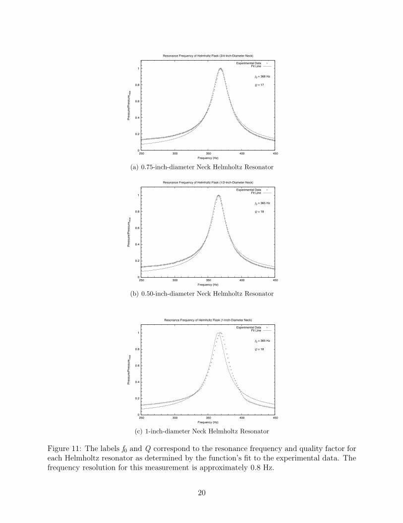
The results of these tuning experiments can be viewed in Figure 11. From Figure 11 one

can see a discrepancy between the experimental data and the fit line. Although this method

of tuning the resonator o"ers a fairly accurate resonance frequency, another method was

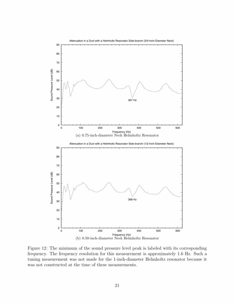
devised in order to increase that accuracy. The experimental duct was set up as described in

Section 3.2 with the speaker replacing the fan at the end of the duct. The speaker projected

white noise into the duct, each Helmholtz resonator was individually introduced into the

duct’s lid, and the sound pressure level was recorded. The results are shown in Figure 12.

could achieve a minimum height of 12 in and a maximum height of 127

8 in, the frequency ranges were limitedto: 64-549 Hz for the 1

2 -inch-diameter-neck Helmholtz resonator; 87-751 Hz for the 34 -inch-diameter-neck

Helmholtz resonator; and 182-925 Hz for the 1-inch-diameter-neck Helmholtz resonator. These limitedfrequency ranges were considered when selecting which fan-produced tonal peak would be attenuated forthis project. Note that these ranges are predicted via Equation 2 and have not been experimentally proven.

11The quality factor of a Helmholtz resonator is defined as "0mR , where !0 is the angular resonance

frequency, m is the mass of air in th neck, and R is the mechanical resistance. Higher quality factorscorrespond to narrow resonance curves whereas lower quality factors correspond to broader resonance curves.

19

0

0.2

0.4

0.6

0.8

1

250 300 350 400 450

Pres

sure

/Pre

ssur

e max

Frequency (Hz)

Resonance Frequency of Helmholtz Flask (3/4-Inch-Diameter Neck)

f0 = 368 Hz

Q = 17

Experimental DataFit Line

(a) 0.75-inch-diameter Neck Helmholtz Resonator

0

0.2

0.4

0.6

0.8

1

250 300 350 400 450

Pres

sure

/Pre

ssur

e max

Frequency (Hz)

Resonance Frequency of Helmholtz Flask (1/2-Inch-Diameter Neck)

f0 = 365 Hz

Q = 18


(b) 0.50-inch-diameter Neck Helmholtz Resonator

0

0.2

0.4

0.6

0.8

1

250 300 350 400 450

Pres

sure

/Pre

ssur

e max

Frequency (Hz)

Resonance Frequency of Helmholtz Flask (1-Inch-Diameter Neck)

f0 = 365 Hz

Q = 18


(c) 1-inch-diameter Neck Helmholtz Resonator

Figure 11: The labels f0 and Q correspond to the resonance frequency and quality factor foreach Helmholtz resonator as determined by the function’s fit to the experimental data. Thefrequency resolution for this measurement is approximately 0.8 Hz.

20

0

10

20

30

40

50

60

70

80

90

0 100 200 300 400 500 600

Soun

d Pr

essu

re L

evel

(dB)

Frequency (Hz)

Attenuation in a Duct with a Helmholtz Resonator Side-branch (3/4-Inch-Diameter Neck)

367 Hz


0

10

20

30

40

50

60

70

80

90

0 100 200 300 400 500 600

Soun

d Pr

essu

re L

evel

(dB)

Frequency (Hz)

Attenuation in a Duct with a Helmholtz Resonator Side-branch (1/2-Inch-Diameter Neck)

368 Hz


Figure 12: The minimum of the sound pressure level peak is labeled with its correspondingfrequency. The frequency resolution for this measurement is approximately 1.6 Hz. Such atuning measurement was not made for the 1-inch-diameter Helmholtz resonator because itwas not constructed at the time of these measurements.

21

3.4 Insertion Loss

-10

-5

0

5

10

15

20

250 300 350 400 450

Soun

d Pr

essu

re L

evel

(dB)

Frequency (Hz)

Insertion Loss 366 Hz in a Duct with a Helmholtz Resonator Side-branch


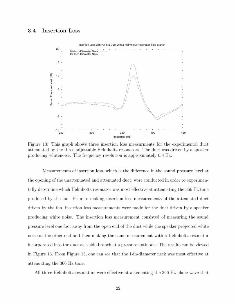
Figure 13: This graph shows three insertion loss measurments for the experimental ductattenuated by the three adjustable Helmholtz resonators. The duct was driven by a speakerproducing whitenoise. The frequency resolution is approximately 0.8 Hz.

Measurements of insertion loss, which is the di"erence in the sound pressure level at

the opening of the unattenuated and attenuated duct, were conducted in order to experimen-

tally determine which Helmholtz resonator was most e"ective at attenuating the 366 Hz tone

produced by the fan. Prior to making insertion loss measurements of the attenuated duct

driven by the fan, insertion loss measurements were made for the duct driven by a speaker

producing white noise. The insertion loss measurement consisted of measuring the sound

pressure level one foot away from the open end of the duct while the speaker projected white

noise at the other end and then making the same measurement with a Helmholtz resonator

incorporated into the duct as a side-branch at a pressure antinode. The results can be viewed

in Figure 13. From Figure 13, one can see that the 1-in-diameter neck was most e"ective at

attenuating the 366 Hz tone.

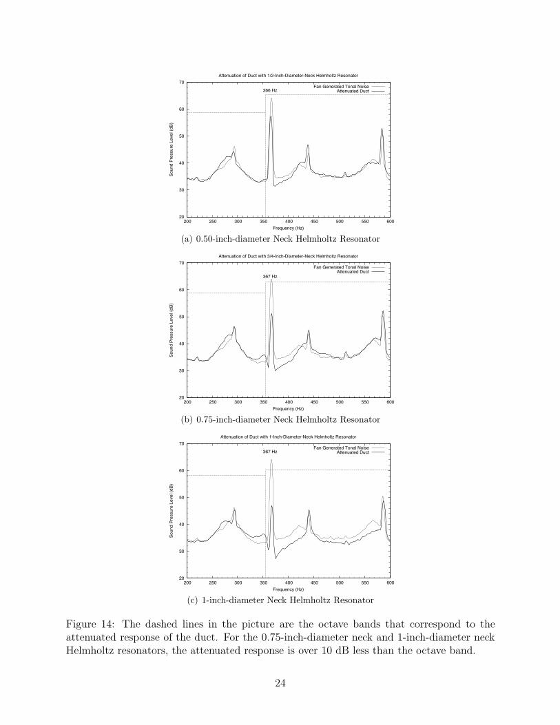
All three Helmholtz resonators were e"ective at attenuating the 366 Hz plane wave that

22

was introduced into the duct by the speaker; however, the acoustic waves introduced into the

duct by the ventilation fan were not uniform like those produced by the speaker. Therefore,

it was uncertain how e"ective the Helmholtz resonators would be a attentuating the tonal

noise produced by the fan. Figure 14 shows the attenuation for the duct with each of the

Helmholtz resonators. Like Figure 13, the 1-inch-diameter neck Helmholtz resonator was

most e"ective at attenuating the tone. However, unlike Figure 14, the insertion loss of the

duct with tonal noise produced by the fan was much greater than than the insertion loss of

the duct with the speaker producing the 366 Hz tone. These results can be seen in Figure

15.

4 Conclusion

4.1 Project Conclusions

When designing a Helmholtz resonator to attenuate tonal noise generated by a fan in a

duct, there are several factors to consider. First, in order to have the greatest attenuation,

a Helmholtz resonator that is introduced adjacently to a duct should be placed such that its

opening corresponds to a pressure antinode (or maximum pressure) of the duct. Secondly,

the Helmholtz resonator must be tuned as precisely as possible to allow for maximum at-

tenuation. One must also consider the acoustic waves produced by the fan are not constant,

plane waves such as those produced by a speaker. Therefore, the transmission loss in a duct

driven by a speaker is not adequate for the transmission loss in a duct driven by a fan.

Based on the results of this project, the transmission loss predications calculated for this

experiment were not an adequate substition for insertion loss predictions. Future projects

would need to explore other prediction methods and suggestions for these new predictions

can be viewed in the following section. However, the predicitions did o"er valuable insight as

to which resonator would be most e"ective at attenuating the unwanted 366 Hz tonal peak.

As predicted, the 1-inch-neck Helmholtz resonator had the greatest attenuation of the tone

23

20

30

40

50

60

70

200 250 300 350 400 450 500 550 600

Soun

d Pr

essu

re L

evel

(dB)

Frequency (Hz)

Attenuation of Duct with 1/2-Inch-Diameter-Neck Helmholtz Resonator

366 HzFan Generated Tonal Noise

Attenuated Duct


20

30

40

50

60

70

200 250 300 350 400 450 500 550 600

Soun

d Pr

essu

re L

evel

(dB)

Frequency (Hz)

Attenuation of Duct with 3/4-Inch-Diameter-Neck Helmholtz Resonator

367 Hz

Fan Generated Tonal NoiseAttenuated Duct


20

30

40

50

60

70

200 250 300 350 400 450 500 550 600

Soun

d Pr

essu

re L

evel

(dB)

Frequency (Hz)

Attenuation of Duct with 1-Inch-Diameter-Neck Helmholtz Resonator

367 HzFan Generated Tonal Noise

Attenuated Duct


Figure 14: The dashed lines in the picture are the octave bands that correspond to theattenuated response of the duct. For the 0.75-inch-diameter neck and 1-inch-diameter neckHelmholtz resonators, the attenuated response is over 10 dB less than the octave band.

24

-10

-5

0

5

10

15

20

200 250 300 350 400 450 500 550 600

Inse

rtion

Los

s (d

B)

Frequency (Hz)

Insertion Loss of Attenuated Duct with 1/2-Inch-Diameter-Neck Helmholtz Resonator

370 Hz


-10

-5

0

5

10

15

20

200 250 300 350 400 450 500 550 600

Inse

rtion

Los

s (d

B)

Frequency (Hz)

Insertion Loss of Attenuated Duct with 3/4-Inch-Diameter-Neck Helmholtz Resonator

363 Hz


-10

-5

0

5

10

15

20

25

200 250 300 350 400 450 500 550 600

Inse

rtion

Los

s (d

B)

Frequency (Hz)

Insertion Loss of Attenuated Duct with 1-Inch-Diameter-Neck Helmholtz Resonator

364 Hz


Figure 15: Insertion loss graphs for each Helmholtz resonator. The 1-in-Helmholtz resonantorwas greatest at attenuating the tonal noise. Note that the greatest insertion loss for eachresonator did not occur at the resonator’s resonance frequency- 366 Hz.

25

whereas the 0.5-inch-neck Helmholtz resonator had the least attenuation.

4.2 Future Experiments

Based on the results shown in Figures 14 and 15, the transmission loss measurements

made in Section 1.4 were accurate in predicting the most e"ective Helmholtz resonator; how-

ever, these predictions are not accurate in predicting insertion loss. Therefore, it is necessary

to adjust these predictions for more accurate results. The adjustment to these predictions

can be accomplished in two di"erent ways. The first method involves experimentally deter-

mining the source’s impedance and calculating insertion loss measurements using Beranek

and Ver’s definition for insertion loss.[4]

The second method involves using a grazing flow prediction for transmission loss where

the Mach number, M, does not equal zero. If this prediction were to be calculated, then it

would be necessary to make actual transmission loss measurements with the duct. Two 12

in holes were drilled in the centers of two of the 3 116 in by 61

8 lids. The holes would allow

for two Larson Davis 12 in microphones to be placed in each lid, and each lid could then be

placed on opposite sides of the Helmholtz resonator. The transmission loss could then be

calculated based on the pressure responses recorded by the microphone.

Designing and creating various Helmholtz resonators would also be a useful extension to

this project. One would need to be mindful of the limited space aboard the ISS during the

design process. It might also be useful to consider lining a Helmholtz resonator’s interior with

acoustic lining. The lining would change the impedance of the neck and cavity, thus allowing

for greater attenuation over a broader range of frequencies. Predictions for acoustically-lined

Helmholtz resonators would need to be further researched.

26

4.3 Acknowledgements

I am very grateful to the following people for their support and encouragement:

Sue Hawkins and her colleagues at the Arkansas Space Grant Consortium for informing

and granting me the opportunity to intern in the Acoustics O!ce at Johnson Space

Center.

My mentor, Chris Allen, who proposed this project to me and guided me during its

ten week duration.

Je"rey Dornak, who was essential in the construction of my experimental setup and

greatly contributed to the success of this project.

Dave Welsh, who taught me my first signal processing lesson as well as o"ered invalu-

able advice in acoustical engineering and measurement methods.

S. Reynold Chu and Shuo Wang, who provided me with resources and support.

Punan Tang, who o"ered me invaluable and practical advice on the incorporation of

Helmholtz resonators into ducts.

Efram Reeves, who initially designed this experiment and willfully helped me with my

questions.

William Slaton, who served as my faculty mentor for this project and o"ered valuable

advice and support.

27

Appendix A:Determining the Fan Speed of a 4184/2XH ebmpapst4100N Series Tubeaxial Fan

The rotational speed of the fan was assumed to be linearly proportional to the voltage

supplied to the fan. At a nominal voltage of twenty-four volts, the fan was stated to have

a speed of 4400 rotations per minute.[8] This fact, along with the knowledge that the fan

speed was zero rpm when no power was supplied to the fan, was used to generate a linear

fit as shown in Figure 16 below. A summary of this relationship can also be viewed in Table

4. Therefore, it was possible to estimate the speed of the fan if the voltage supplied to the

fan was known.

0

500

1000

1500

2000

2500

3000

3500

4000

4500

0 5 10 15 20 25

Fan

Spee

d (m

in-1

)

Voltage (Volts)

Fan Speed as a Function of Voltage

y = 183.33x

Figure 16: Assuming that the fan speed is linearly proportional to the voltage suppliedto the fan, it is possible to use known information from the fan’s specifications sheet todetermine the proportionality constant. Multiplying the voltage by this constant shouldyield an approximation to the fan’s speed.

28

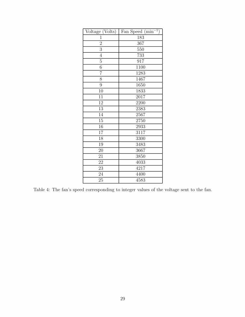
Voltage (Volts) Fan Speed (min"1)1 1832 3673 5504 7335 9176 11007 12838 14679 165010 183311 201712 220013 238314 256715 275016 293317 311718 330019 348320 366721 385022 403323 421724 440025 4583

Table 4: The fan’s speed corresponding to integer values of the voltage sent to the fan.

29

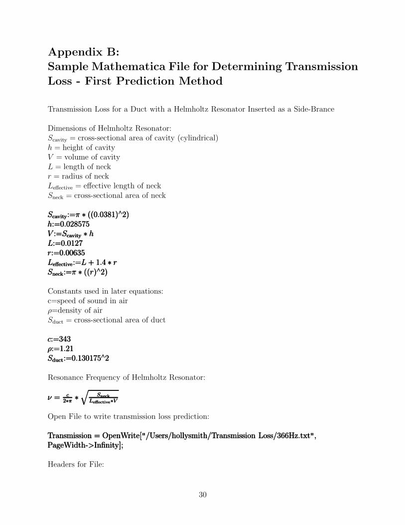
Appendix B:Sample Mathematica File for Determining TransmissionLoss - First Prediction Method

Transmission Loss for a Duct with a Helmholtz Resonator Inserted as a Side-Brance

Dimensions of Helmholtz Resonator:Scavity = cross-sectional area of cavity (cylindrical)h = height of cavityV = volume of cavityL = length of neckr = radius of neckLe"ective = e"ective length of neckSneck = cross-sectional area of neck

Scavity:=" " ((0.0381)#2)Scavity:=" " ((0.0381)#2)Scavity:=" " ((0.0381)#2)h:=0.028575h:=0.028575h:=0.028575V :=Scavity " hV :=Scavity " hV :=Scavity " hL:=0.0127L:=0.0127L:=0.0127r:=0.00635r:=0.00635r:=0.00635Le"ective:=L + 1.4 " rLe"ective:=L + 1.4 " rLe"ective:=L + 1.4 " rSneck:=" " ((r)#2)Sneck:=" " ((r)#2)Sneck:=" " ((r)#2)

Constants used in later equations:c=speed of sound in air#=density of airSduct = cross-sectional area of duct

c:=343c:=343c:=343#:=1.21#:=1.21#:=1.21Sduct:=0.130175#2Sduct:=0.130175#2Sduct:=0.130175#2

Resonance Frequency of Helmholtz Resonator:

! = c2$# "

2Sneck

Le!ective$V! = c

2$# "2

SneckLe!ective$V! = c

2$# "2

SneckLe!ective$V

Open File to write transmission loss prediction:

Transmission = OpenWrite["/Users/hollysmith/Transmission Loss/366Hz.txt",Transmission = OpenWrite["/Users/hollysmith/Transmission Loss/366Hz.txt",Transmission = OpenWrite["/Users/hollysmith/Transmission Loss/366Hz.txt",PageWidth->Infinity];PageWidth->Infinity];PageWidth->Infinity];

Headers for File:

30

Write[Transmission, {"Frequency [Hz]", "Transmission Loss"}];Write[Transmission, {"Frequency [Hz]", "Transmission Loss"}];Write[Transmission, {"Frequency [Hz]", "Transmission Loss"}];

Calculations for the File:x= 1

T"

TL=10 log10

"1

T"

#

The Do Loop is continued for a frequency range of 200 Hz - 500 Hz, and the frequency andtransmission loss are written to the file ’366Hz.txt’.

Do[Do[Do[

x = 1 +

-c

2"Sduct

$$“

2"""i"Le!ectiveSneck

" c2

2"""i"V

”

.2;x = 1 +

-c

2"Sduct

$$“


" c2

2"""i"V

”

.2;x = 1 +

-c

2"Sduct

$$“


" c2

2"""i"V

”

.2;

TL = 10 " Log[10, x];TL = 10 " Log[10, x];TL = 10 " Log[10, x];Write[Transmission, {i, TL}]Write[Transmission, {i, TL}]Write[Transmission, {i, TL}], {i, 200, 500, 1}];, {i, 200, 500, 1}];, {i, 200, 500, 1}];

Closing the file:

Close[Transmission]Close[Transmission]Close[Transmission]

31

Appendix C:Sample Mathematica File for Determining TransmissionLoss - Second Prediction Method

Clearing Stored Symbols:

Clear["Global*"]Clear["Global*"]Clear["Global*"]

Transmission Loss for a Duct with a Helmholtz Resonator Inserted as a Side-Brance

Dimensions of Helmholtz Resonator:# = density of airc = speed of sound in airrn = radius of neckSn = cross-sectional aread of neckLn = length of neck%n = neck correctionV = volumeSd = cros-sectional area of ductrc = radius of cavity (cylindrical)h = height of cavity

#:=1.21#:=1.21#:=1.21c:=343c:=343c:=343rn:=0.00635rn:=0.00635rn:=0.00635Sn:=" " (rn

2)Sn:=" " (rn2)Sn:=" " (rn2)

Ln:=0.0127Ln:=0.0127Ln:=0.0127%n:=1.4 " rn%n:=1.4 " rn%n:=1.4 " rn

V :=0.00013031V :=0.00013031V :=0.00013031Sd:=0.1301752Sd:=0.1301752Sd:=0.1301752

rc:=0.0381rc:=0.0381rc:=0.0381h:=0.028575h:=0.028575h:=0.028575

Resonance Frequency of Helmholtz Resonator:

! = c2$# "

2Sn

(Ln+%n)$V! = c2$# "

2Sn

(Ln+%n)$V! = c2$# "

2Sn

(Ln+%n)$V

Open File to Write Transmission Loss:

Transmission = OpenWrite["/Users/hollysmith/NewTL.txt",Transmission = OpenWrite["/Users/hollysmith/NewTL.txt",Transmission = OpenWrite["/Users/hollysmith/NewTL.txt",

32

PageWidth->Infinity];PageWidth->Infinity];PageWidth->Infinity];

Headers for File:

Write[Transmission, {"Frequency [Hz]", "Transmission Loss"}];Write[Transmission, {"Frequency [Hz]", "Transmission Loss"}];Write[Transmission, {"Frequency [Hz]", "Transmission Loss"}];

Calculations for the File:

Do[Do[Do[k = 2$#$i

c ;k = 2$#$ic ;k = 2$#$ic ;

x = Abs

$

%%%%&

2+“

!"cSd

”$

0

B@ 1

i"

c""r2

c

!"Cot[ 2"""i

c "h]+( c"k2" #i" c"k(Ln+1.4"rn)

Sn )

1

CA

2

'

(((();x = Abs

$

%%%%&

2+“

!"cSd

”$

0

B@ 1

i"

c""r2

c

!"Cot[ 2"""i

c "h]+( c"k2" #i" c"k(Ln+1.4"rn)

Sn )

1

CA

2

'

(((();x = Abs

$

%%%%&

2+“

!"cSd

”$

0

B@ 1

i"

c""r2

c

!"Cot[ 2"""i

c "h]+( c"k2" #i" c"k(Ln+1.4"rn)

Sn )

1

CA

2

'

(((();

TL = 20 " Log[10, x];TL = 20 " Log[10, x];TL = 20 " Log[10, x];Write[Transmission, {i, TL}]Write[Transmission, {i, TL}]Write[Transmission, {i, TL}], {i, 0, 10000, 1}];, {i, 0, 10000, 1}];, {i, 0, 10000, 1}];

Closing the file:

Close[Transmission]Close[Transmission]Close[Transmission]

33

References

[1] Goodman, Jerry R. “International Space Station Acoustics.” Proceedings of Noise-Con2003. Cleveland, Ohio. 23-25 June 2003.

[2] Spratlin, Larry. “CQ Acoustics Assessment Report for CDR.” June 27, 2008.

[3] “CQ Project Technical Requirements Specification for the ISS Crew Quarters,” Revi-sion A. Engineering Directorate, Crew and Thermal Systems Division, Johnson SpaceCenter, June 25, 2007.

[4] Beranek, Leo L. and Ver, Istvan L. Noise and Vibration Control Engineering. JohnWiley & Sons, New York, NY, 1992.

[5] Orr, W. Graham. Handbook for Industrial Noise Control. The Bionetics Corporation,Hampton, Virginia, 1981.

[6] L.E. Kinsler, A.R. Frey, A.B. Coppens, and J.V. Sanders. Fundamentals of Acoustics,4th edition. John Wiley & Sons, New York, NY, 1982.

[7] Seo, Sang-Hyun and Kim, Yang-Hann. “Silencer design by using array resonators forlow-frequency band noise reduction,” Journal of the Acoustical Society of America, 118,2332-2338 (2005).

[8] “DC Axial Fans Specification Sheet.” ebmpapst. http://www.ebmpapst.co.uk/Assets/PDF/Press\%20Releases/Serie\%204100N_GB.pdf.

34

Reduction of Fan Generated Tonal Noise in a Ventilation...

Documents

Transcript of Reduction of Fan Generated Tonal Noise in a Ventilation...