Recursive MUSIC: A Framework for EEG and MEG …neuroimage.usc.edu/paperspdf/R_Music2.pdfRecursive...
40
Recursive MUSIC: A Framework for EEG and MEG Source Localization John C. Mosher * and Richard M. Leahy + * Los Alamos National Laboratory Group P-21 MS D454 Los Alamos, NM 87545 USA (505) 665-2175 voice, (505) 665-4507 fax email: [email protected] + Signal & Image Processing Institute University of Southern California Los Angeles, CA 90089-2564 USA (213) 740-4659 voice, (213) 740-4651 fax email: [email protected] Los Alamos Technical Report: LA-UR-97-3182 and USC-SIPI Report No. 304 (Revision of Los Alamos Technical Report: LA-UR-96-3829) This technical report has been revised and submitted for review and possible publication in a journal. Because changes may be made before publication, this document is made available with the understanding that any journal version supersedes this document. Until such journal publica- tion occurs, please cite this work using the above technical report numbers.
Transcript of Recursive MUSIC: A Framework for EEG and MEG …neuroimage.usc.edu/paperspdf/R_Music2.pdfRecursive...
Recursive MUSIC: A Framework forEEG and MEG Source Localization
John C. Mosher* and Richard M. Leahy+
*Los Alamos National LaboratoryGroup P-21 MS D454
Los Alamos, NM 87545 USA(505) 665-2175 voice, (505) 665-4507 fax
email: [email protected]+Signal & Image Processing Institute
University of Southern CaliforniaLos Angeles, CA 90089-2564 USA
(213) 740-4659 voice, (213) 740-4651 faxemail: [email protected]
Los Alamos Technical Report: LA-UR-97-3182and
USC-SIPI Report No. 304
(Revision of Los Alamos Technical Report: LA-UR-96-3829)
This technical report has been revised and submitted for review and possible publication in a
journal. Because changes may be made before publication, this document is made available with
the understanding that any journal version supersedes this document. Until such journal publica-
tion occurs, please cite this work using the above technical report numbers.
Mosher, Leahy: R-MUSIC Version 2 Page 2 of 40
Los Alamos Technical Report # LA-UR-97-3182 July 31, 1997
Recursive MUSIC: A Frameworkfor EEG and MEG Source Localization‡
John C. Mosher* and Richard M. Leahy+
*Los Alamos National Laboratory, Group P-21 MS D454,Los Alamos, NM 87545 [email protected], (505) 665-2175
+Signal & Image Processing Institute, University of Southern California,Los Angeles, CA 90089-2564 [email protected], (213) 740-4659
The multiple signal classification (MUSIC) algorithm can be used to locate multiple asynchro-
nous dipolar sources from electroencephalography (EEG) and magnetoencephalography (MEG)
data. The algorithm scans a single dipole model through a three-dimensional head volume and
computes projections onto an estimated signal subspace. To locate the sources, the user must
search the head volume for multiple local peaks in the projection metric. This task is time consum-
ing and subjective. Here we describe an extension of this approach which we refer to as recursive
MUSIC (R-MUSIC). This new procedure automatically extracts the locations of the sources
through a recursive use of subspace projections. The new method is also able to locate synchronous
sources through the use of a spatio-temporal independent topographies (IT) model. This model
defines a source as one or more non-rotating dipoles with a single time course. Within this frame-
work, we are able to locate fixed, rotating and synchronous dipoles. The recursive subspace pro-
jection procedure that we introduce here uses the metric of principal correlations as a
multidimensional form of correlation analysis between the model subspace and the data subspace.
By recursively computing principal correlations, we build up a model for the sources that account
for a given set of data. We demonstrate here how R-MUSIC can easily extract multiple asynchro-
nous dipolar sources that are difficult to find using the original MUSIC scan. We then demonstrate
R-MUSIC applied to the more general IT model and show results for combinations of fixed, rotat-
ing, and synchronous dipoles.
‡This work was supported in part by the National Institute of Mental Health Grant R01-MH53213, by the National
Eye Institute Grant R01-EY08610-04, and by Los Alamos National Laboratory, operated by the University of
California for the United States Department of Energy under contract W-7405-ENG-36.
Mosher, Leahy: R-MUSIC Version 2 Page 3 of 40
Los Alamos Technical Report # LA-UR-97-3182 July 31, 1997
I. I NTRODUCTION
The problem of localizing the sources of event related scalp potentials (the electroencephalo-
gram or EEG) and magnetic fields (the magnetoencephalogram or MEG) can be formulated in
terms of finding a least-squares fit of a set of current dipoles to the observed data. Early attempts
at source localization were based on fitting the multiple dipole model to a single time sample of the
measurements across the E/MEG (EEG and/or MEG) array[5], [23], [33]. By noting that physio-
logical models for the current sources typically assume that they are spatially fixed for the duration
of a particular response, researchers were able to justify fitting the multiple dipole model to a com-
plete spatio-temporal data set[2], [3], [19], [20]. The spatio-temporal model can result in substan-
tial improvements in localization accuracy; however, processing the entire data set leads to a large
increase in the number of unknown parameters, since the times series for each source must now be
estimated in addition to the dipole location and orientation. We show in[12] that since these time
series parameters are linear with respect to the data, they can be factored out and the source loca-
tions found without explicit computation of their associated time series.
While factoring out the linear parameters can reduce the dimensionality of the search required
to localize the sources of the measured fields, a fundamental problem remains: the least-squares
cost function is highly non-convex with respect to the locations of the dipoles. Consequently,
inverse methods such as gradient-based optimization or simplex searches often become trapped in
local minima, yielding significant localization errors (cf.[9]). In an attempt to overcome this prob-
lem, we have examined the use of signal subspace methods that are common in the array signal
processing literature[10]. The method that we used in[12], which was originally referred to as the
MUSIC (for MUltiple SIgnal Classification) algorithm in[21], replaces the multiple dipole
directed search with a procedure in which a single dipole is scanned through a grid confined to a
three-dimensional head or source volume. At each point on this grid, the forward model for a dipole
at this location is projected against a signal subspace that has been computed from the E/MEG data.
The locations on this grid where the source model gives the best projection onto the signal subspace
correspond to the dipole locations. We also show in[12] that we do not need to test all possible
Mosher, Leahy: R-MUSIC Version 2 Page 4 of 40
Los Alamos Technical Report # LA-UR-97-3182 July 31, 1997
dipole orientations at each location, but instead can solve a generalized eigenvalue problem whose
solution gives us the orientation of the dipole which gives the best fit to the signal subspace for a
source at that location.
One of the major problems with the MUSIC method, and one that is addressed by the new
approach described here, is how we choose the locations which give the best projection on to the
signal subspace. In the absence of noise and with perfect head and sensor models, the forward
model for a source at the correct location will project entirely into the signal subspace. In practice,
of course, there are errors in the estimate of the signal subspace due to noise, and there are errors
in the forward model due to approximations in our models of the head and data acquisition system.
An additional problem is that we often compute the metric only at a finite set of grid points. The
effect of these practical limitations is that the user is faced with the problem of searching the grid-
ded source volume for “peaks” and deciding which of these peaks correspond to true locations. It
is important to note that a local peak in this metric does not necessarily indicate the location of a
source. Only when the forward model projects entirely into the signal subspace – or as close as one
would expect given errors due to noise and model mismatch – can we infer that a source is at that
location. The effect of this limitation is that some degree of subjective interpretation of the MUSIC
“scan” is required to decide on the locations of the sources. This subjective interpretation is clearly
undesirable and can also lead to the temptation to incorrectly view the MUSIC scan as an image
whose intensity is proportional to the probability of a source being present at each location.
Two other problems that arise with the use of MUSIC are based on the assumptions that the
data are produced by a set of asynchronous dipolar sources and that the data are corrupted by addi-
tive spatially-white noise. Often both of these assumptions are incorrect in clinical or experimental
data. If two dipoles have synchronous activation, then the two-dimensional signal subspace that
would have been produced if they were asynchronous collapses into a one dimensional subspace.
Scanning of a single dipole against this subspace using MUSIC will fail to localize either of the
sources. The new MUSIC algorithm described here is able to localize synchronous sources through
the use of a modified source representation, which we refer to as the spatio-temporalindependent
Mosher, Leahy: R-MUSIC Version 2 Page 5 of 40
Los Alamos Technical Report # LA-UR-97-3182 July 31, 1997
topographies (IT) model. This model is described in detail inSection II. The second problem, the
issue of non-white noise, is not addressed in depth here. We note, however, that it is straightforward
to modify both the original and R-MUSIC algorithms to cope with colored noise through standard
pre-whitening procedures[25]. In practice, the pre-whitening could be achieved by using pre-stim-
ulus data to estimate the covariance of the background noise; see[22], [24] as recent examples of
processing E/MEG data with colored noise.
We begin the paper inSection II with a combined formulation of the E/MEG forward problem
in which we develop a standard matrix notation for the relationship between the source and data.
We then describe the spatio-temporal independent topographies model in which, rather than treat-
ing individual current dipoles as sources, we define a source as one or more non-rotating dipoles
with a single time course. In this way our model is constrained to consist of a number of sources
equal to the rank of the signal subspace. InSection III we review the definition and properties of
the signal subspace and relate these subspaces to cost functions commonly used for estimating the
parameters of the model. We describe the use of principal correlations as a general metric for com-
puting the goodness of fit of putative sources to the signal subspace. We then review the MUSIC
algorithm in the light of the preceding development. The new R-MUSIC algorithm is then devel-
oped inSection IV. We present some examples of the application of R-MUSIC to fixed, rotating
and synchronous dipolar sources inSection V. A condensed version of this paper appears in[17]‡.
II. SPATIO -TEMPORAL INDEPENDENT TOPOGRAPHIES
A. Background
Quasi-static approximations of Maxwell’s equations govern the relationship between neural
current sources and the E/MEG data that they produce. For the signal subspace methods for source
localization that are described here, these relationships must be expressed in matrix form. In[15]
we reviewed matrix forms of the “lead field”[4], [29] for EEG and MEG measurements, for both
‡In [11], [17], we referred to R-MUSIC as RAP-MUSIC; we have since adopted the terminol-
ogy used here and in[18] to differentiate the two methods.
Mosher, Leahy: R-MUSIC Version 2 Page 6 of 40
Los Alamos Technical Report # LA-UR-97-3182 July 31, 1997
spherical and general BEM head models. In each case, the measurements can be expressed as an
explicit function ofprimary currentactivity; thepassive volume currents due to the macroscopic
electric fields are implicitly embedded in the lead field formula. The lead field should also account
for the sensor characteristics of the measurement modality, such as gradiometer orientation and
configuration in MEG or differential pairs in EEG. The result is that our EEG or MEG measure-
ment at sensor location may be expressed as
(1)
where is the volume of sources, represents theprimary current density at any point in
the volume, and is thelead field vector[4], [29] relating the sensor point to the primary
current point. The scalar function represents either the voltage potential or the magnetic field
component that may be observed at observation (sensor) point .
If we assume that the primary current exists only at a discrete point , i.e., the primary current
is , where is the Dirac delta functional, then(1) simplifies in E/MEG to
(2)
where is themoment of acurrent dipolelocated at .We assume in this paper that our source
consists of current dipole sources. We assume simultaneous recordings at sensors for time
instances. We can express the by spatio-temporal data matrix as
. (3)
or
. (4)
f m r( ) r
f m r( ) g r r ′,( ) j r ′( )⋅ r ′dV∫=
V j r ′( ) r ′
g r r ′,( )
f m r( )
r
rq
j r ′( )δ r ′ rq–( ) δ r ′ rq–( )
f m r( ) g r rq,( ) q⋅=
q rq
p m n
m n
f m r1 t1,( ) … f m r1 tn,( )
… … …f m rm t1,( ) … f m rm tn,( )
g r1 rq1,( )T … g r1 rqp,( )
T
… … …
g rm rq1,( )T … g rm rqp,( )
T
q1 t1( ) … q1 tn( )
… … …qp t1( ) … qp tn( )
=
Fm G rq1( ) … G rqp( ) QT=
Mosher, Leahy: R-MUSIC Version 2 Page 7 of 40
Los Alamos Technical Report # LA-UR-97-3182 July 31, 1997
We refer to as the dipole “gain matrix”[12] that maps a dipole at into a set of mea-
surements. The three columns of the gain matrix represent the possibleforward fieldsthat may be
generated by the three orthogonal orientations of the th dipole at the sensor locations
. Each row of the full gain matrix represents thelead fieldsam-
pled at the discrete dipole locations . The matrix is ourspatio-temporal model
matrix of perfect measured data, i.e., the magnetic field component or scalp potential data we
would observe in the absence of noise.
The columns of represent the time series associated with each of the three orthogonal com-
ponents of each dipole, i.e., with each column of the gain matrix. For the “fixed” dipole model,
whose moment orientation is time invariant, we can separate the orientation of each source from
the moments as[12]:
(5)
such that , where is a unit norm orientation vector. The scalar time series
are thelinear parameters of our model, the corresponding dipole locations are thenon-
linear parameters, and the dipole orientations are thequasi-linearparameters.
In [12], we also considered a “rotating” dipole as one whose time series could not be decom-
posed into a single fixed orientation and time series and therefore comprised multiple “elemental”
dipoles. Physically, a rotating dipole may be viewed as two nearly collocated dipoles with indepen-
dent time series, such that they are indistinguishable from a model comprising a single dipole
whose orientation is allowed to vary with time. The “hybrid” models in[12] comprised both fixed
and rotating dipoles.
G rqi( ) rqi
i m
r1 … rm, ,{ } G rq1( ) … G rqp( )
rq1 … rqp, ,{ } Fm
Q
Fm G rq1( ) … G rqp( )
uq1 0
…0 uqp
sq1 t1( ) … sq1 tn( )
… … …sqp t1( ) … sqp tn( )
=
qi ti( ) uqisqi ti( )= uqi
sqi ti( ) rqi
uqi
Mosher, Leahy: R-MUSIC Version 2 Page 8 of 40
Los Alamos Technical Report # LA-UR-97-3182 July 31, 1997
B. Independent Topographies
A common observation in MUSIC processing is that the rank of the signal subspace should
equal the number of “sources.” As defined in[12], we allowed a source to be a single dipole with
one (“fixed”) or more (“rotating”) independent time courses. For example, the data model defined
by (5) assumes a collection of “fixed” dipoles. The MUSIC method applied to this model
requires that all dipoles have linearly independent time courses. Stated conversely, each linearly
independent time course is associated with a single dipole.
Our goal in this section is build up a new source model for the data as the sum of contributions
from a fixed number of spatio-temporalindependent topographies. Each of these independent
topographies (ITs) is considered to be a source comprising one or more fixed dipoles which collec-
tively have a single time course. Thus, in contrast to our models in[12], each linearly independent
time course is now associated with oneor more dipoles. By building up the model in this way, the
rank of the signal subspace is, by definition, always equal to the number of sources. This represen-
tation then provides a convenient framework for describing and implementing our new variant of
the MUSIC algorithm.
We cluster the dipoles into subsets and restate(4) as where
represents sets of dipoles. The th set of dipoles comprises dipoles with
the location parameter set . The moments of the th set are clustered such that,
by design, theymust result in a rank-one time series matrix. An SVD of these moments yields
(6)
p
p r Fm G ρ( )Q=
ρ ρ1 … ρr, ,{ }≡ r i ρi pi
ρi rq1i( ) … rqpi
i( ), ,
≡ i
QiT
q1i( )
t1( ) … q1i( )
tn( )
… … …
qpi
i( )t1( ) … qpi
i( )tn( )
uiσiviT
= =
Mosher, Leahy: R-MUSIC Version 2 Page 9 of 40
Los Alamos Technical Report # LA-UR-97-3182 July 31, 1997
where and are respectively the left and right singular vectors of unit norm, and is the only
non-zero singular value of the decomposition of . The result is that the th set of dipoles may
be represented by the rank one spatio-temporal matrix
(7)
where the time series follows from the decomposition in(6) as .
The sets of dipoles are then collected such that(4) is now restated as
(8)
(9)
where the set contains the corresponding unit norm vectors. Our final require-
ment in this IT framework is that must be of rank , and therefore, by necessity, both
and are of full column rank . We refer to each column vector of as a “ -dipolar inde-
pendent topography,” with a corresponding time series found as the th column of .
Through the IT framework, we have altered the original concept of spatio-temporal source
modeling[20]. If written as(4), we might state that our model comprises dipolar sources with
their corresponding time series; however, such a viewpoint has led to the complexity of represent-
ing “fixed” and “rotating” or “regional” dipoles. The rank of this spatio-temporal dipolar model
spanned from unity (i.e., all dipoles fixed and synchronous) to (e.g., fully rotating dipoles in an
EEG model). The number of “sources” depended on the viewpoint of the researcher, since some
viewed the rotating dipole as a single “regional” source or as multiple “elemental” sources. When
written as(9), we have altered the spatio-temporal model by stating that the number of sourcesmust
equal the rank of the spatio-temporal model, where a single source may now comprise one or more
ui vi σi
Qi i
G ρi( )QiT
G rq1i( )
( ) … G rqpi
i( )( ) uiσivi
T a ρi ui,( )siT
= =
si σivi=
r
Fm G ρ( )Q a ρ1 u1,( ) … a ρr ur,( )
s1T
…
srT
= =
A ρ θ,( )ST=
θ u1 … ur, ,{ }≡
Fm r A ρ θ,( )
S r A ρ θ,( ) pi
i S
p
3p
Mosher, Leahy: R-MUSIC Version 2 Page 10 of 40
Los Alamos Technical Report # LA-UR-97-3182 July 31, 1997
dipoles. Each source generates a “topography” across the array of sensors that is spatially and tem-
porally independent of any other source or topography.
We will conclude this section with some examples that show the relationships between IT mod-
els and common multiple dipole models. The case of three fixed dipoles, with asynchronous time
series, is represented by the rank-three spatio-temporal matrix as
(10)
where is the set of dipole locations and is the set of dipole
orientations as shown in(5). Our IT model is said to comprise three “single-dipolar topographies.”
Now consider the case where two of these dipoles are synchronous, but the third remains asynchro-
nous from the others. The rank of the model is two, and our IT model must be adjusted to account
for two sources,
(11)
where now is the set of source locations, and the second source comprises two
dipoles, . The set of source orientations is , and we may continue to
view as the orientation of the dipole in the single-dipole topography. The orientation , how-
ever, is a generalized form of source orientation and is in this instance a six-dimensional vector, as
discussed inthe Appendix. The first three elements of this vector relate to the orientation of dipole
and similarly the second set of three elements relate to . The norm of the first three elements
gives the strength of dipole relative to , with the restriction that the combined vector of all
elements in is of unit norm. This IT model comprises one “single-dipolar” topography and one
“2-dipolar” topography.
If all three dipoles are synchronous, then our IT model comprises a single “3-dipolar” topog-
raphy. Similarly, we consider the limiting case of a single time slice and a general dipole model;
A ρ θ,( )ST a rq1 uq1,( ) a rq2 uq2,( ) a rq3 uq3,( ), ,[ ] sq1 sq2 sq3, ,[ ]T=
ρ rq1 rq2 rq3, ,{ }≡ θ uq1 uq2 uq3, ,{ }≡
A ρ θ,( )ST a rq1 uq1,( ) a ρ2 u2,( ),[ ] sq1 s2,[ ]T=
ρ rq1 ρ2,{ }≡
ρ2 rq2 rq3,{ }≡ θ uq1 u2,{ }≡
uq1 u2
rq2 rq3
rq2 rq3
u2
p
Mosher, Leahy: R-MUSIC Version 2 Page 11 of 40
Los Alamos Technical Report # LA-UR-97-3182 July 31, 1997
this spatio-temporal model is always rank one, and our IT model is therefore a single -dipolar
topography.
“Rotating” or “regional” dipoles are a simple extension of the IT framework. In the case of the
MEG spherical head model, a single “rotating” dipole becomes two fixed orientation dipoles cor-
responding to two “single-dipolar” topographies,
(12)
with . In other words, two fixed dipoles share the same location, just different ori-
entations and time courses, which is the original intent of a “rotating” model. For other head mod-
els, the dipole may possibly rotate in three dimensions, . Note that the
(or ) IT gain matrix (or )
properly remains of full column rank.
To summarize, all “sources” in an IT model must be mutually spatially and temporally inde-
pendent. Under this requirement, therankof the noiseless spatio-temporal data matrix determines
the number of independent topographies. Each topography in turn may comprise multiple dipoles
with synchronous time courses. The IT model can handle arbitrary combinations of synchronous
and asynchronous, and fixed and rotating dipoles.
III. S IGNAL SUBSPACE METHODS
A. Signal Subspaces
We will now investigate the relationship between the IT model and the signal subspace that we
estimate from the spatio-temporal data. Assume that a random noise matrix comprising time
slices is added to the data , to produce an “noisy”
spatio-temporal data set,
(13)
p
A ρ θ,( )ST a ρ1 uq1,( ) a ρ2 uq2,( ),[ ] sq1 sq2,[ ]T=
ρ1 ρ2 rq1= =
ρ1 ρ2 ρ3 rq1= = = m 2×
m 3× a rq1 uq1,( ) a rq1 uq2,( ) a rq1 uq1,( ) a rq1 uq2,( ) a rq1 uq3,( )
n
N n t1( ) … n tn( )≡ Fm A ρ θ,( )ST= m n×
F AST N+=
Mosher, Leahy: R-MUSIC Version 2 Page 12 of 40
Los Alamos Technical Report # LA-UR-97-3182 July 31, 1997
For convenience we will drop the explicit dependence of on its parameters. The goal of the
inverse problem is to estimate the parameters, , given the data set . We will use the
common assumption that the noise is zero-mean and white, i.e., , where
denotes the expected value of the argument, and is the identity matrix. The case for col-
ored noise is readily treated with standard pre-whitening methods[25], provided a reasonable esti-
mate of the noise covariance is available. For event related studies, the noise covariance can
probably be estimated using sufficiently long periods of pre-stimulus data.
Under the zero-mean white noise assumption, we may represent the expected value of the
matrix outer product as
(14)
(15)
Here we have assumed that our model parameters and the dipolar time series are deterministic.
From our independent topographies model, we know that is rank and may be eigen-
decomposed as , where contain the eigenvectors such that = ,
and is the corresponding diagonal matrix of nonzero eigenvalues.
We can eigendecompose the correlation matrix as
. (16)
(17)
where is the diagonal matrix combining both the model and noise eigenval-
ues, and is the diagonal matrix of noise only eigenvalues. The
A
ρ θ S, ,{ } F
n ti( )n ti( )T{ }E σn
2I=
•{ }E I
FF T
RF FF T{ }E≡ ASTSATE n ti( )nT
ti( )( )i 1=
n
∑+=
ASTSATnσN
2 I+=
ASTSATr
ΦsΛΦsT Φs m r× spanΦs( ) spanA( )
Λ r r×
RF Φs Φn,[ ]Λ nσN
2 I+ 0
0 nσN2 I
Φs Φn,[ ]T=
ΦsΛsΦsT ΦnΛnΦn
T+=
Λs Λ nσN2 I+≡ r r×
Λn nσN2 I≡ m r–( ) m r–( )×
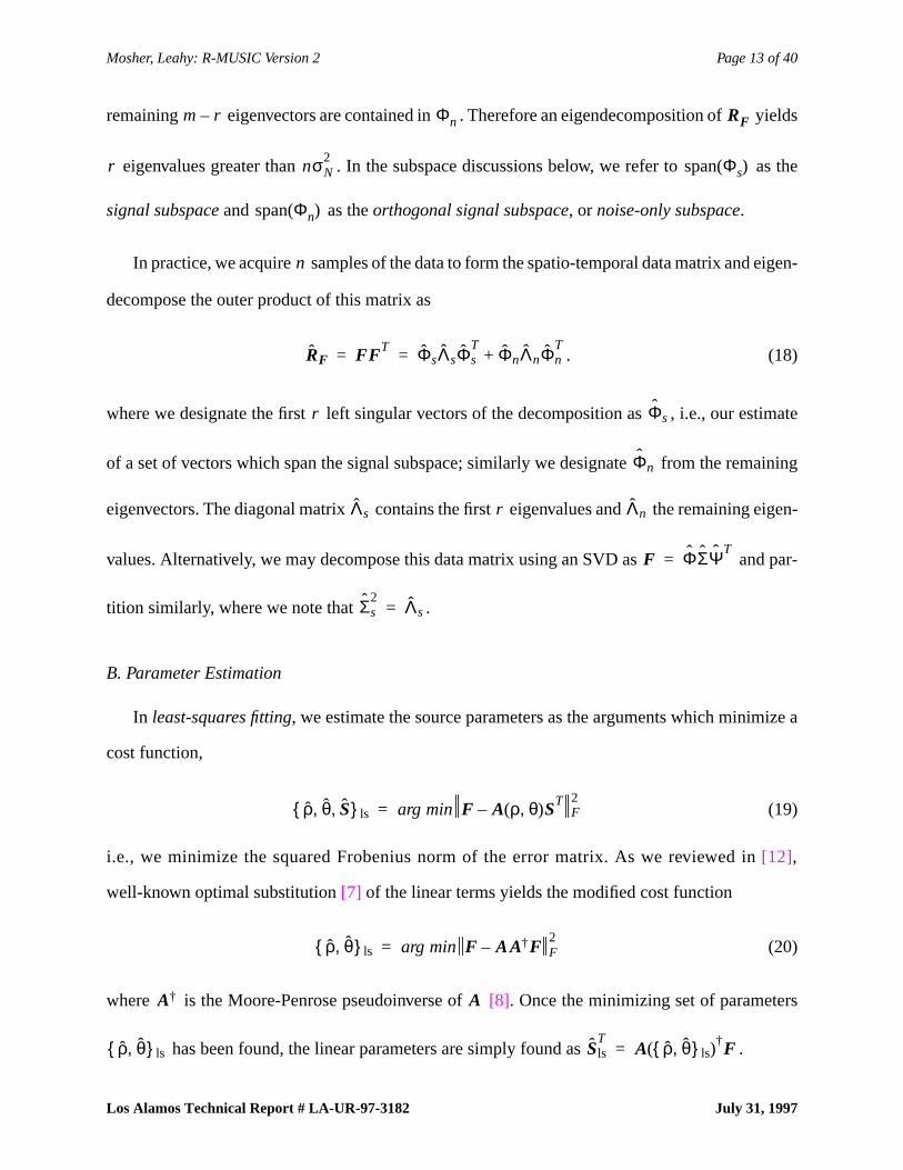
Mosher, Leahy: R-MUSIC Version 2 Page 13 of 40
Los Alamos Technical Report # LA-UR-97-3182 July 31, 1997
remaining eigenvectors are contained in . Therefore an eigendecomposition of yields
eigenvalues greater than . In the subspace discussions below, we refer to as the
signal subspaceand as theorthogonal signal subspace, ornoise-only subspace.
In practice, we acquire samples of the data to form the spatio-temporal data matrix and eigen-
decompose the outer product of this matrix as
. (18)
where we designate the first left singular vectors of the decomposition as , i.e., our estimate
of a set of vectors which span the signal subspace; similarly we designate from the remaining
eigenvectors. The diagonal matrix contains the first eigenvalues and the remaining eigen-
values. Alternatively, we may decompose this data matrix using an SVD as and par-
tition similarly, where we note that .
B. Parameter Estimation
In least-squares fitting, we estimate the source parameters as the arguments which minimize a
cost function,
(19)
i.e., we minimize the squared Frobenius norm of the error matrix. As we reviewed in[12],
well-known optimal substitution[7] of the linear terms yields the modified cost function
(20)
where is the Moore-Penrose pseudoinverse of[8]. Once the minimizing set of parameters
has been found, the linear parameters are simply found as .
m r– Φn RF
r nσN2
spanΦs( )
spanΦn( )
n
RF FF T ΦsΛsΦsT
ΦnΛnΦnT
+= =
r Φs
Φn
Λs r Λn
F ΦΣΨT=
Σs2
Λs=
ρ θ S, ,{ }ls F A ρ θ,( )ST– F
2arg min=
ρ θ,{ }ls F AA†F– F2
arg min=
A† A
ρ θ,{ }ls SlsT
A ρ θ,{ }ls( )†F=
Mosher, Leahy: R-MUSIC Version 2 Page 14 of 40
Los Alamos Technical Report # LA-UR-97-3182 July 31, 1997
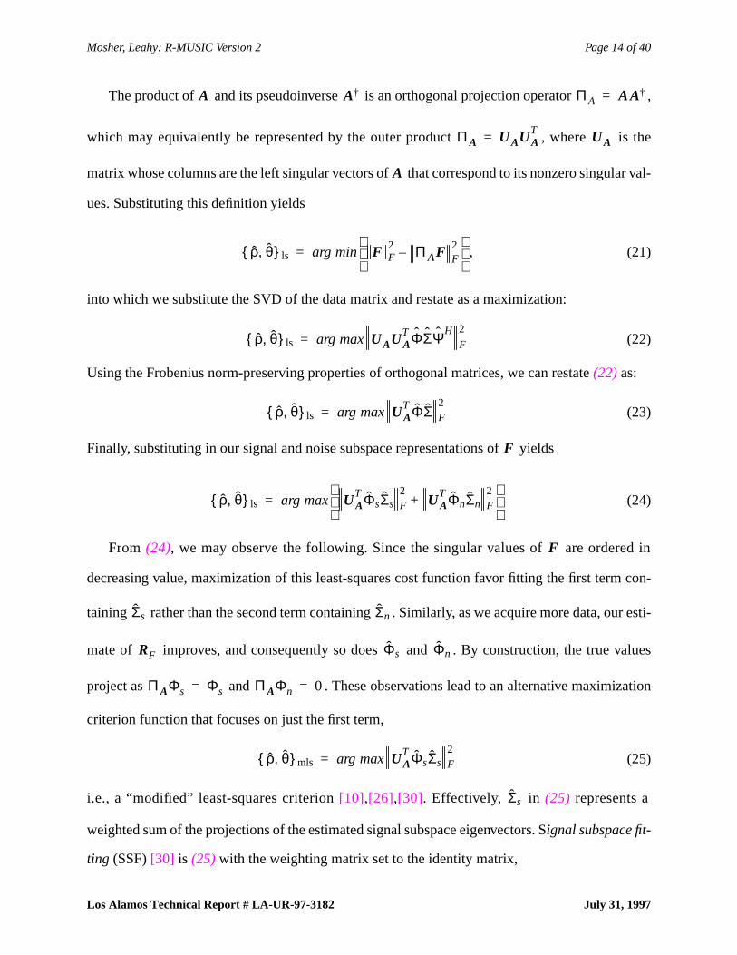
The product of and its pseudoinverse is an orthogonal projection operator ,
which may equivalently be represented by the outer product , where is the
matrix whose columns are the left singular vectors of that correspond to its nonzero singular val-
ues. Substituting this definition yields
, (21)
into which we substitute the SVD of the data matrix and restate as a maximization:
(22)
Using the Frobenius norm-preserving properties of orthogonal matrices, we can restate(22) as:
(23)
Finally, substituting in our signal and noise subspace representations of yields
(24)
From (24), we may observe the following. Since the singular values of are ordered in
decreasing value, maximization of this least-squares cost function favor fitting the first term con-
taining rather than the second term containing . Similarly, as we acquire more data, our esti-
mate of improves, and consequently so does and . By construction, the true values
project as and . These observations lead to an alternative maximization
criterion function that focuses on just the first term,
(25)
i.e., a “modified” least-squares criterion[10],[26],[30]. Effectively, in (25) represents a
weighted sum of the projections of the estimated signal subspace eigenvectors. Signal subspace fit-
ting (SSF)[30] is (25) with the weighting matrix set to the identity matrix,
A A† ΠA AA†=
ΠA UAUAT
= UA
A
ρ θ,{ }ls F F2 ΠAF F
2–
arg min=
ρ θ,{ }ls UAUAT ΦΣΨH
F
2arg max=
ρ θ,{ }ls UAT ΦΣ F
2arg max=
F
ρ θ,{ }ls UAT ΦsΣs F
2UA
T ΦnΣn F
2+
arg max=
F
Σs Σn
RF Φs Φn
ΠAΦs Φs= ΠAΦn 0=
ρ θ,{ }mls UAT ΦsΣs F
2arg max=
Σs
Mosher, Leahy: R-MUSIC Version 2 Page 15 of 40
Los Alamos Technical Report # LA-UR-97-3182 July 31, 1997
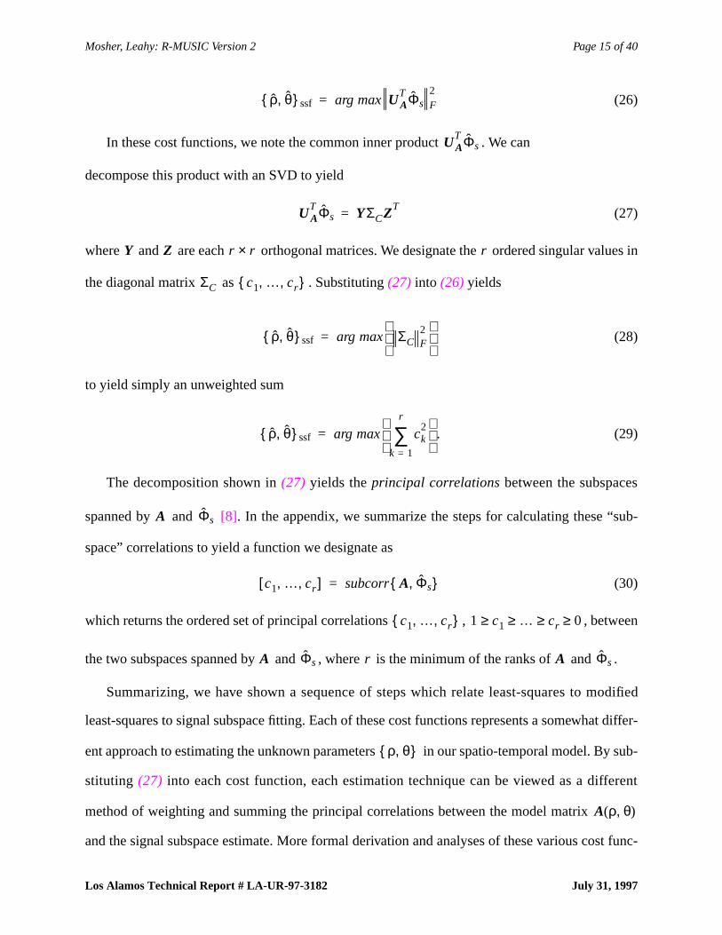
(26)
In these cost functions, we note the common inner product . We can
decompose this product with an SVD to yield
(27)
where and are each orthogonal matrices. We designate the ordered singular values in
the diagonal matrix as . Substituting(27) into (26) yields
(28)
to yield simply an unweighted sum
. (29)
The decomposition shown in(27) yields theprincipal correlationsbetween the subspaces
spanned by and [8]. In the appendix, we summarize the steps for calculating these “sub-
space” correlations to yield a function we designate as
(30)
which returns the ordered set of principal correlations , , between
the two subspaces spanned by and , where is the minimum of the ranks of and .
Summarizing, we have shown a sequence of steps which relate least-squares to modified
least-squares to signal subspace fitting. Each of these cost functions represents a somewhat differ-
ent approach to estimating the unknown parameters in our spatio-temporal model. By sub-
stituting (27) into each cost function, each estimation technique can be viewed as a different
method of weighting and summing the principal correlations between the model matrix
and the signal subspace estimate. More formal derivation and analyses of these various cost func-
ρ θ,{ }ssf UAT Φs F
2arg max=
UAT Φs
UAT Φs YΣCZT
=
Y Z r r× r
ΣC c1 … cr, ,{ }
ρ θ,{ }ssf ΣC F2
arg max=
ρ θ,{ }ssf ck2
k 1=
r
∑
arg max=
A Φs
c1 … cr, ,[ ] A Φs,{ }subcorr=
c1 … cr, ,{ } 1 c1 … cr 0≥ ≥ ≥ ≥
A Φs r A Φs
ρ θ,{ }
A ρ θ,( )
Mosher, Leahy: R-MUSIC Version 2 Page 16 of 40
Los Alamos Technical Report # LA-UR-97-3182 July 31, 1997
tions in relation to the general array signal processing problem may be found in[26], [27], [30],
[31], [32]. We will now use the novel framework of principal correlations to re-develop the MUSIC
algorithm and introduce our new variant, R-MUSIC.
C. MUSIC
The least-squares and SSF methods reviewed above require nonlinear multidimensional
searches to find the unknown parameters . MUSIC was introduced by Schmidt[21] as a
means to reduce the complexity of this nonlinear search. Here we review MUSIC in terms of the
principal correlations, which in turn leads to our proposed R-MUSIC approach.
Given that the rank of is and the rank of is at least , the smallest principal cor-
relation value,
, (31)
represents the minimum principal correlation (maximum principal angle) between principal vec-
tors in the column space of and the signal subspace . The principal correlation of any
individual column with the signal subspace must therefore equal or exceed this
minimum principal correlation,
, (32)
As the quality of our signal subspace estimate improves (either by improved signal to noise
ratios or longer data acquisition), then will approach and the minimum correlation
approaches unity when the correct parameter set is identified, such that the distinct sets
of parameters have principal correlations approaching unity. Thus a search strategy for
identifying the parameter set is to identify peaks of the met-
ric
(33)
ρ θ,{ }
A ρ θ,( ) r Φs r
cr A ρ θ,( ) Φs,{ }subcorrmin≡
A ρ θ,( ) Φs
a ρi θi,( ) A ρ θ,( )∈
a ρi θi,( ) Φs,{ }subcorr A ρ θ,( ) Φs,{ }subcorrmin≥ i 1 … r, ,=
Φs Φs
ρ θ,{ } r
ρi θi,{ }
ρ θ,{ } ρ1 θ1,{ } … ρr θr,{ }, ,{ }= r
a ρ θ,( ) Φs,{ }subcorr2aT ρ θ,( )ΦsΦs
Ta ρ θ,( )
a ρ θ,( )2
---------------------------------------------------=
Mosher, Leahy: R-MUSIC Version 2 Page 17 of 40
Los Alamos Technical Report # LA-UR-97-3182 July 31, 1997
where the squaredsubcorr operation is readily equated with the right hand side, since the first argu-
ment is a vector and the second argument is already a matrix with orthonormal columns. We rec-
ognize this as the MUSIC metric[21], with the minor difference of using the signal subspace
projector rather than the more commonly used noise-only subspace projector . If our
estimate of the signal subspace is perfect, then we will find global maxima equal to unity.
D. Quasi-linear Solution
Before proceeding to a description of MUSIC, we first address the problem of finding the ori-
entation vector . The dipole parameters are chosen to maximize
(34)
However, , a vector constrained to unity norm, represents a linear combination of the columns
of the gain matrix (see equation(6) and preceding discussion). We can avoid explicitly
searching for the optimal orientation vector by noting that the maximum of the principal correlation
vector gives us the best way of combining the columns of so that they
are as close as possible to the signal subspace. Therefore we can find the dipole locations by solving
(34) at each candidate dipole location, then searching for the locations at which this maximum cor-
relation equals, or is sufficiently close to, unity. Once we find these locations, we can then explicitly
find the corresponding best orientation as “ ” (see Appendix) scaled to unity norm.
E. Classical MUSIC
In [12] we adapted a “diversely polarized” form of Schmidt’s original MUSIC algorithm[6],
[21] to the problem of multiple point dipoles. We briefly review and update that presentation here
to include our discussion of principal correlations. The steps are:
1. Obtain a spatio-temporal data matrix , comprising information from sensors and
time slices. Decompose or and select the rank of the signal subspace to obtain
ΦsΦsH
ΦnΦnH
r
ui
a ρi ui,( ) Φs,{ }subcorr
ui
G ρi( )
G ρi( ) Φs,{ }subcorr G ρi( )
x1
F m
n F FF T
Mosher, Leahy: R-MUSIC Version 2 Page 18 of 40
Los Alamos Technical Report # LA-UR-97-3182 July 31, 1997
. Overspecifying the true rank by a couple of dimensions usually has little effect on per-
formance. Underspecifying the rank can dramatically reduce the performance.
2. Create a relatively dense grid of dipolar source locations. At each grid point, form the
gain matrix for the dipole. At each grid point, calculate the principal correlations
.
3. As a graphical aid, plot the inverse of , where is the maximum principal
correlation. Correlations close to unity will exhibit sharp peaks (indeed, perfect correlation
yields an infinite spike). Locate or fewer peaks in the grid. At each peak, refine the search
grid to improve the location accuracy, and check the second principal correlation. A large
second principal correlation is an indication of a “rotating dipole.”
IV. R-MUSIC
Problems with the use of MUSIC arise when there are errors in the estimate of the signal sub-
space and the principal correlation is computed at only a finite set of grid points. The largest peak
is usually easily located by searching over the grid for the largest correlation; however, the second
and subsequent peaks must be located by means of a three-dimensional “peak-picking” routine.
The R-MUSIC methods overcomes this problem by recursively building up the IT model and com-
paring this full model to the signal subspace.
A. Development
In the following we assume that our independent topographies each comprise one or more
dipoles. We search first for the single dipolar topographies, then the two-dipolar topographies, and
so forth. As we discover each topography model, we add it to our existing IT model and continue
the search. We build the source model by recursively applying the principal correlation measure,
the key metric of MUSIC, to successive principal correlations.
Φs
G
G Φs,{ }subcorr
1 c12
– c1
r
Mosher, Leahy: R-MUSIC Version 2 Page 19 of 40
Los Alamos Technical Report # LA-UR-97-3182 July 31, 1997
For exemplary purposes, we first assume that the independent topographies each comprise a
single dipole. Single dipole locations are readily found by scanning the head volume. At each point
in the volume, we calculate
(35)
where is the set of principal correlations. We find the dipole location which max-
imizes the primary correlation . As described inthe Appendix, the corresponding dipole orien-
tation is easily obtained from , and we designate our topography model
comprising this first dipole as
(36)
To search for the second dipole, we again search the head volume; however, at each point in the
head, we first form the model matrix . We then calculate
(37)
but now we find the dipole point that maximizes thesecondprincipal correlation, ; the first prin-
cipal correlation should already account for in the model. The corresponding dipole ori-
entation may be readily obtained by projecting this second topography against the subspace,
, and we append this to our model to form
. (38)
We repeat the process times, maximizing the th principal correlation at the th pass,
. The final iteration is effectively attempting to minimize the subspace “distance”[8]
between the full topographies matrix and the signal subspace estimate.
If the topographies comprise single-dipolar topographies and 2-dipolar topographies,
then R-MUSIC will first extract the single dipolar models. At the th iteration, we will
r
c1 c2 …, ,{ } G rq( ) Φs,{ }subcorr=
c1 c2 …, ,{ } rq1
c1
u1 G rq1( ) Φs,{ }subcorr
A1( )
a rq1 u1,( )=
M A1( )
G rq( ),[ ]=
c1 c2 …, ,{ } M Φs,{ }subcorr=
c2
a rq1 u1,( )
u2
G rq2( ) Φs,{ }subcorr
A2( )
a rq1 u1,( ) a rq2 u2,( ),[ ]=
r k k
k 1 … r, ,=
r
r r1 r2
r1 r1 1+( )
Mosher, Leahy: R-MUSIC Version 2 Page 20 of 40
Los Alamos Technical Report # LA-UR-97-3182 July 31, 1997
find no single dipole location that correlates well with the subspace. We then increase the number
of dipole elements per topography to two. We must now search simultaneously for two dipole loca-
tions, such that
(39)
is maximized for the principal correlation , where comprises two dipoles. If
the combinatorics are not impractical, we can exhaustively form all pairs on our grid and compute
maximum principal correlations for each pair. The alternative is to begin a two-dipole nonlinear
search with random initialization points to maximize this correlation (cf.[9]). This low-order
dipole search can be easily performed using standard minimization methods.
We proceed in this manner to build the remaining 2-dipolar topographies. As each pair of
dipoles is found to maximize the appropriate principal correlation, the corresponding pair of dipole
orientations may be readily obtained from , as described inthe Appendix.
Extensions to more dipoles per independent topography are straightforward, although the complex-
ity of the search obviously increases. In any event, the complexity of the search will always remain
less than or equal to the least-squares search required for finding all dipoles simultaneously.
B. Algorithm
To summarize, we assume that our forward model has been corrupted by additive noise, and
that this noise is zero mean with a known spatial covariance matrix . We decompose or
and select the rank of the signal subspace to form , which is our estimate of a set of vectors
that span the signal subspace. If the rank is uncertain, we should err towards overspecifying the
signal subspace rank. If we overselect the rank, the additional subspace vectors should span an arbi-
trary subspace of the noise-only subspace, and the probability that these vectors correlate with our
model is small; hence, we may in general overspecify the rank of the signal subspace. However, as
the overspecification of the signal subspace increases, so does the probability that we may inad-
c1 c2 …, ,{ } Ar 1( )
G ρ( ),[ ] Φs,
subcorr=
cr 1 1+ ρ rq1 rq2,{ }=
r2
G ρ( ) Φs,{ }subcorr
σn2I F FF T
r Φs
Mosher, Leahy: R-MUSIC Version 2 Page 21 of 40
Los Alamos Technical Report # LA-UR-97-3182 July 31, 1997
vertently include a noise-only subspace that correlates with our models, so some prudence is called
for in rank selection. We demonstrate examples of overselection of the subspace inSection V.
We design a sufficiently dense grid in our volume of interest, and at each grid point we form
the head model for the single dipole gain matrix .We initialize the topography complexity as
“1-dipolar topography,” i.e., each topography comprises a single dipole. We then proceed as fol-
lows:
1. Forindexfrom 1 to rank :
2. Let be the model extracted as of the previous loop ( is a
null matrix for the first loop).
3. Form sets of grid points , where for a 1-dipolar topography each set consists of the
location of a single grid point . For a 2-dipolar topography, contains the locations of
pairs of grid points, and so on for higher order dipolar topographies. If the combinatorics
make it impractical to consider all possible combinations of grid points, choose a random
subset of the possible combinations.
4. For each set of grid points , form the grid model , i.e., concate-
nate the set of grid point models to the present extracted model.
5. Calculate the set of principal correlations, , using
the algorithm described inthe Appendix.
6. Find the maximum over all sets of grid points for , e.g., for , find
the maximumsecondprincipal correlation.
7. Optionally, if the set of grid points is not particularly dense or complete, then
use a nonlinear optimization method (e.g., Nelder-Meade simplex) to maximize ,
beginning the optimization at the best . If the grid is dense and our sets in Step 2 com-
plete, this step may not be necessary.
l i
G l i( )
r
A a1 … a index 1–( ), ,[ ]= A
λi
l i λi
λi M i A G λi( ),[ ]=
c1 c2 …, ,{ } M i Φs,{ }subcorr=
λi cindex index 2=
λi{ }
cindex
λi
Mosher, Leahy: R-MUSIC Version 2 Page 22 of 40
Los Alamos Technical Report # LA-UR-97-3182 July 31, 1997
8. Is the correlation at the location of the maximum “sufficient,” i.e., does indi-
cate a good correlation? If the correlation is adequate, proceed to Step 11. If it is not, pro-
ceed to Step 9.
9. (Insufficient correlation in Step 8). We have two situations to consider. We may have
overspecified the true rank of the signal subspace, in which case we are now attempting to
fit a topography into a noise-only subspace component. We can test for this condition by
forming the projection operator (where is thepseudoinverse[12]) from the
existing estimated model, then forming the residual . Inspection and test-
ing of the residual should reveal whether or not we believe a signal is still present. If we
believe the residual is simply “noise,” break this loop. Otherwise, proceed to Step 10.
10. (Signal still apparent in the residual) Increase the complexity of the topography
(e.g. from one to two dipolar) and return to Step 3 without increasing the loopindex.
11. (Good correlation in Step 8) We have found the best set of locations of the
next independent topography, with corresponding gain matrix . We need the
best fitting orientation. Calculate the principal orientation vector (seethe Appendix)
from , normalize , and form the topography
vector .
12. Increment theindex and loop to Step 1 for the next independent topography.
In Step 8, we recommend here that the correlation exceed at least 95%. In[14], we discuss
some of the means for determining if a MUSIC peak represents “adequate” or “sufficient” correla-
tion. Our recommendation here of 95% reflects the empiricism that a “good” solution should gen-
erate a topography which explains at least 90% (the square of the correlation, i.e., the “R-squared”
statistic) of the variance of the topography identified in the data. If we overselect the rank of the
signal subspace, then we will in general break out of the loops at Step 9, once we have found the
cindex
PA
A A†
= A†
F res F PA
F–=
ρindex
Gindex ρindex( )
x1
Gindex ρindex( ) Φs,{ }subcorr uindex x1 x1⁄=
aindex Gindex ρindex( )uindex=

Mosher, Leahy: R-MUSIC Version 2 Page 23 of 40
Los Alamos Technical Report # LA-UR-97-3182 July 31, 1997
true number of sources and have only noise left in the residual. We will not address the determina-
tion of statistical “sufficiency” of the model in this paper. The interested reader may refer to ([1],
[28]) among others for discussions on the testing of the residual for remnant signals.
If the grid is dense or we performed Step 7 for each topography, we may find the R-MUSIC set
of parameters is already a good solution. The R-MUSIC algorithm has maximized a set of principal
correlations, a metric different from the least-squares approach. We may refine this solution with a
least-squares search:
13. Our R-MUSIC search has yielded an estimate of the full spatial topographies gain
matrix , which is a function of the estimated full set of dipole locations
and orientations . Beginning with these parameters, initialize a nonlinear search using
the cost functions(24) or (25).
Step 13 represents an increase in the complexity in the nonlinear search over that of R-MUSIC,
at possibly diminishing returns in terms of improvement in the solution. Note that each iteration of
the nonlinear search must now adjust the parameters of all of the dipoles, not just a single topog-
raphy as in R-MUSIC.
V. COMPUTER SIMULATIONS
We present two simulations to illustrate some of the features of our proposed IT model and the
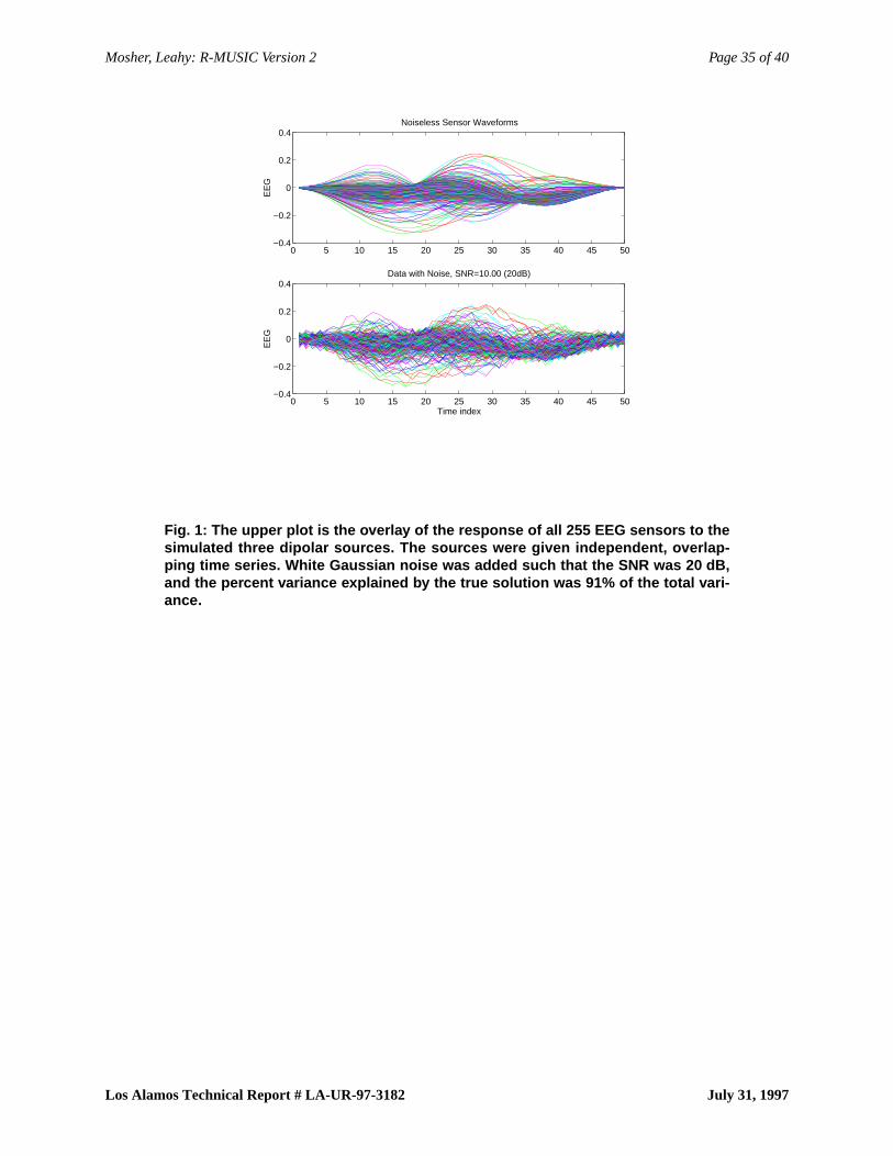
R-MUSIC algorithm. In the first simulation, we arranged 255 EEG sensors about the upper region
of an 8.8 cm single shell sphere, with a nominal spacing between sensors of 1 cm. For illustrative
purposes, we arranged three dipolar sources in the same plane, cm, and the three sources
were given independent, overlapping time courses. The overlay of the responses of all sensors is
given in the upper plot ofFig. 1. We then added white Gaussian noise to all data points, scaled such
that the squared Frobenius norm of the noise matrix was one-tenth that of the squared Frobenius
norm of the noiseless signal matrix, for an SNR of 20 dB. The lower plot ofFig. 1 shows the over-
lay of all sensors for the signal plus noise data.
A a1 … ar, ,[ ]=
ρ θ
z 7=

Mosher, Leahy: R-MUSIC Version 2 Page 24 of 40
Los Alamos Technical Report # LA-UR-97-3182 July 31, 1997
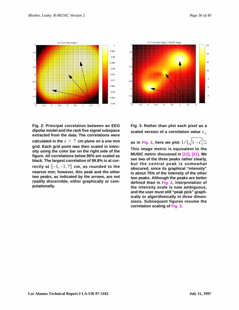
The singular value spectrum was clearly rank three, but we selected rank five to illustrate
robustness to rank over-selection. We created a 1 mm grid in the cm plane and calculated
the correlation between a single dipole model and the signal subspace.Fig. 2 displays these corre-
lation as an image whose intensities are proportional to the primary correlation . We have defined
the gray scale inFig. 2 such that the principal correlation must exceed 95% in order to be visible.
In Fig. 3, we have replotted the same data, but in this case we plot in order to graph-
ically intensify the appearance of the peaks. This image is the original MUSIC scan proposed in
[12]. The measure is equivalent to the correlation with the noise-only subspace, the orig-
inal proposal by Schmidt[21]. As we discussed in[12], plotting the inverse of this measure makes
graphical location of the peaks easier; however, since that publication we have found it more infor-
mative to plot the principal correlation, since correlation is a direct measure of how well the model
fits the data.
The largest principal correlation of 99.8% is easily found at cm, as rounded to the
nearest mm. The peak at is apparent inFig. 3, but the peak at is obscured in both
figures (see caption). Graphically or computationally declaring the location of these other two
peaks is non-obvious without subjective interpretation by the observer.
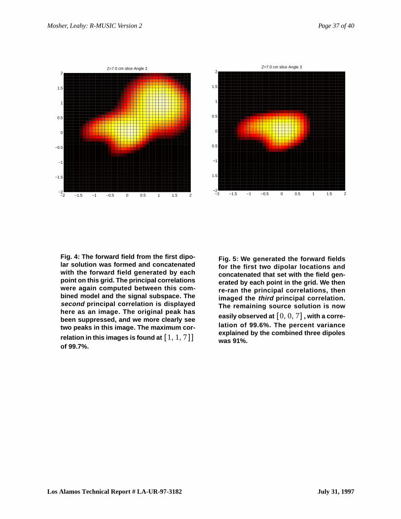
We generated the forward field for this first dipole, then re-scanned the principal correlation on
the same grid with the combined model.Fig. 4 displays thesecond principal correlation; in this and
subsequent figures, we will resume plotting the correlation value directly, rather than the inverted
metric. We can now more clearly see the peaks corresponding to the two remaining sources, and
the first source has been suppressed. The maximum peak of this image at 99.7% is easily located
at .
We then generated the forward field for this second dipole and appended it to the first dipole’s
forward field. We then re-scanned the principal correlations on the same grid with the combined
model.Fig. 5 displays thethird principal correlation, where we now readily observe the single
z 7=
c1
1 1 c12
–( )⁄
1 c12
–
1– 1– 7, ,[ ]
1 1 7, ,[ ] 0 0 7, ,[ ]
1 1 7, ,[ ]
Mosher, Leahy: R-MUSIC Version 2 Page 25 of 40
Los Alamos Technical Report # LA-UR-97-3182 July 31, 1997
remaining peak for the third source, 99.6% at . Visual examination of the residual at this
point indicated no remaining signal, and principal correlations of multiple dipole models yielded
no substantial correlations.
The second simulation was designed to demonstrate the localization of a “rotating” dipole and
a pair of synchronous dipoles, as well as to illustrate the use of a directed search algorithm to refine
these locations. In this simulation, we arranged 240 MEG planar gradiometer sensors about the
upper hemisphere, with a nominal spacing of about 2 cm and a baseline separation of 1 cm. A
“rotating” dipole was located at cm, and a pair of dipoles with synchronous activation was
located at and cm. We then created a 1.5 mm grid in the cm plane,
i.e., in a plane displaced from the true source plane, and the gridding was slightly coarser than the
first simulation. The noise level was again set to 20 dB. The true rank of the signal subspace was
three, with the rotating dipole comprising two single-dipolar topographies, and the third topogra-
phy comprising a two-dipolar topography.Fig. 6 displays the overlay of the noiseless and noisy
sensor responses.
We again overselected the rank of the signal subspace rank to be five, then scanned the one
dipole model against the signal subspace. We found a single good peak at 99.3%, as displayed in
Fig. 7. Note the absence of any other peaks; the remaining “rotating” dipolar topography is
obscured by this peak, and the other topography is not a single dipole. The peak observed in the
grid was at cm. We initiated a directed search from this point to maximize the cor-
relation to 99.8% at cm, the correct solution for the single dipole topography,
rounded to the nearest mm.
As in the previous example, we then scanned for a second dipole, observing the second princi-
pal correlation. The maximum correlation in the grid was again high, 99.2%, at ,
as shown inFig. 8. A directed search initiated at this point maximized the second principal corre-
lation at 99.7% at , the same dipole location as the first solution. The dipole orientations
0 0 7, ,[ ]
0 0 7, ,[ ]
2– 2– 7, ,[ ] 2 2 7, ,[ ] z 6.5=
0.1 0.2– 6.5, ,[ ]
0.0 0.0 7.0, ,[ ]
0.1– 0.2– 6.5, ,[ ]
0 0 7, ,[ ]
Mosher, Leahy: R-MUSIC Version 2 Page 26 of 40
Los Alamos Technical Report # LA-UR-97-3182 July 31, 1997
of the two solutions were nearly orthogonal, and , indicating we had
correctly identified the simulated “rotating” dipole at this point.
We then scanned for a third single dipole solution, but only a peak of 88.8% was found, and a
directed search maximization only improved this correlation to 88.9%. Thus this third dipole could
only account for of the variance of the third topography, and we rejected this
third single dipolar topography solution.
Since one dipole was inadequate to describe the third topography, we shifted to our next puta-
tive solution, that of two dipoles. Our grid comprised 729 dipole locations, and all combinations of
two dipoles yielded 265,356 sets. Rather than exhaustively search all set combinations, we ran-
domly selected a small subset of these sets for a total of about 3,000 sets. We then concatenated
each of these 3,000 pairs with the first two dipole solutions, calculated the principal correlation of
the combined model and observed the third principal correlation. The maximum third correlation
of 98.4% corresponded to the pair at . We initiated a two dipole
directed search from this set and achieved a maximum correlat ion of 99.7% at
cm, the correct solution. InFig. 9, we plot two-dimensional
cross-slices of this six-dimensional function, holding constant the correct plane and the true loca-
tion of one of the two dipoles. We clearly observe the correlation metric peaking at the correct solu-
tion. As in the first example, visual examination of the residual from this model revealed that no
signal was present, and further correlations with multiple dipole models yielded no substantial cor-
relations.
This relatively simple pair of simulations has illustrated some of the key concepts of the
R-MUSIC algorithm and the IT model. Both simulations used relatively dense grids of EEG or
MEG sensors, such that sensor spacing was not an issue; see[13] for analysis of the effects of EEG
and MEG sensor spacing on dipole localization performance. In both simulations, we overselected
the true rank of the signal subspace to illustrate the robustness to such an error; we repeated the
localization results with the true rank and achieved nearly identical results to those presented here.
0.94 0.34 0, ,[ ] 0.3 0.95 0, ,[ ]
88.9%( )2 79.0%=
2– 1.9– 6.5, ,[ ] 1.8 1.8 6.5, ,[ ],
2.0– 2.0– 7.0, ,[ ] 2.0 2.0 7.0, ,[ ],
z
Mosher, Leahy: R-MUSIC Version 2 Page 27 of 40
Los Alamos Technical Report # LA-UR-97-3182 July 31, 1997
In these simulations, as in[12], the subspace scans were presented as images to highlight the
MUSIC peaks; however, the R-MUSIC algorithm readily extracts these peaks without the need for
the user to manually observe and select these solutions. Indeed, in these simulations, the set of
MUSIC peaks would have been difficult to discriminate either graphically or computationally, due
to their proximity and the noise. Additional simulation studies using R-MUSIC can be found in
[11], [17].
In practice, after we have scanned on a discrete grid for any of the single or multiple dipolar
solutions, we always then initiate a directed search from these points to maximize the correlation.
By optimizing the correlation in this manner, we bypass some of the concerns of coarse or inade-
quate gridding. In the first simulation, each of the three dipoles was located with a single dipole
search of three location parameters; in contrast, a full nonlinear least-squares would have required
nine parameters. In the second simulation, we performed two single-dipole searches, followed by
a two-dipole search of six nonlinear parameters. A full nonlinear least-squares search would have
required a twelve parameter search.
VI. C ONCLUSION
In the E/MEG inverse problem, our goal is to estimate a set of parameters that represent our
source. In the multiple dipole model, an issue that complicates the least-squares problem is that it
requires a multidimensional search over a highly non-convex cost function. Here we have
described a new algorithm, R-MUSIC, which uses principal correlations between the model sub-
space and the data subspace to reduce the problem to a sequential search. By identifying one source
at a time we reduce the computational complexity of the search. The search for topographies com-
prising a few dipoles can then be performed over the entire source volume, largely avoiding the
local minima problem.
The independent topography (IT) model that was also presented here is a new framework in
which to view the concept of a source. We often encounter dipolar sources that are effectively fully
correlated in their time courses due to either bisynchronous activation or strong noise. The IT
model allows a straightforward interpretation of these correlated dipoles as a single source topog-
Mosher, Leahy: R-MUSIC Version 2 Page 28 of 40
Los Alamos Technical Report # LA-UR-97-3182 July 31, 1997
raphy comprising multiple dipoles. Combining the R-MUSIC method with the IT source model
keeps the complexity of the parameter search simple relative to more traditional multidimensional
cost functions while bypassing the “peak-picking” problem of the classical MUSIC algorithm.
While determining multiple peaks in a single parameter case (the common presentation in much of
the array signal processing literature on MUSIC) is possible, we found the problem confounding
in even our simplest case of single dipolar topographies, where we must search for peaks in
three-dimensions. Graphically searching for multiple peaks in two-dipolar topographies (a
six-dimensional space) is generally not practical.
In this paper, we have used multiple dipoles as our source model, increasing the independent
topography complexity by simply increasing the number of synchronous dipoles. The IT model
and R-MUSIC algorithm are readily extended to include source models that can represent more
distributed current activity, as we will address in a future publication.
APPENDIX: PRINCIPAL CORRELATION
A. Definitions and Computation
From[8], we summarize the definition and method for computation of the principal or “sub-
space” correlation. Given two matrices, and , where is , and is , let be the
min imum of the ranks o f the two mat r ices . We wish to ca lcu la te a funct ion
, where the scalars are defined as follows.
(40)
subject to:
(41)
The vectors and are theprincipal vectorsbetween the subspaces
spanned by and , and by construction, each set of vectors represents an orthonormal basis.
A B A m p× B m q× r
A B,{ }subcorr c1 c2 … cr, , ,{ }= ck
ck maxa A∈ maxb B∈ aTb akTbk= =
a b 1= =
aTai 0=
bTbi 0=
i 1 … k 1–, ,=
i 1 … k 1–, ,=
a1 … ar, ,{ } b1 … br, ,{ }
A B
Mosher, Leahy: R-MUSIC Version 2 Page 29 of 40
Los Alamos Technical Report # LA-UR-97-3182 July 31, 1997
Note that . The angles are theprincipal angles, representing
the geometric angle between and , or analogously, is theprincipal correlation between
these two vectors. The steps to compute the principal correlations are as follows[8] (p. 585),
1. If and are already orthogonal matrices, we redesignate them as and and
skip to Step 2. Otherwise, perform a singular value decomposition (SVD) of , such that
. Similarly decompose . Retain only those components of and
that correspond to nonzero singular values, i.e., the number of columns in and cor-
respond to their ranks, and the other matrices are square, with dimension equal to the ranks.
2. Form .
3. If only the correlations are desired, then compute only the singular values of (the
extra computation for the singular vectors is not required). The ordered singular values
are the subspace or principal correlations between and .
4. If the principal vectors are also desired, then compute the full singular value decom-
position, . The ordered singular values are extracted from the diagonal of
. Form the sets principal vectors and for sets and
respectively.
The matrices and are each orthogonal, and the columns comprise the ordered sets of
principal vectors for matrices and respectively. If both matrices are of the same subspace
dimension, the measure is called thedistancebetween spaces and [8].
When the distance is zero, we see that and are parallel subspaces. A maximum distance of
unity ( )indicates at least one basis of is orthogonal to or vice versa; if the principal
1 c1 c2 … cr 0≥ ≥ ≥ ≥ ≥ θkcos ck=
ak bk ck
A B UA UB
A
A UAΣAV AT
= B UA UB
UA UB
C UATUB=
C
r
1 c1 c2 … cr 0≥ ≥ ≥ ≥ ≥ A B
C UCΣCVCT
= r
ΣC Ua UAUC= Ub UBVC= A B
Ua Ub
A B
1 cr2
– θrsin= A B
A B
cr 0= A B
Mosher, Leahy: R-MUSIC Version 2 Page 30 of 40
Los Alamos Technical Report # LA-UR-97-3182 July 31, 1997
correlation , then all bases are orthogonal. We see that minimizing the distance is equivalent
to maximizing the minimum principal correlation between and .
We may also readily compute the specific linear combinations of and that yielded these
principal vectors and angles. By construction, we know that for some , and can be
simply found using the pseudoinverse of . If we have used the SVD to decompose , then the
calculation of reduces to ; similarly, we compute .
The best way to linearly combine the columns of (i.e. the combination that minimizes the
angle of the resulting vector with ) is found in the first column of (similarly
define ), , which is best correlated with when it is arranged as . In other
words, there is no other (excepting a scale factor of ) for which a corresponding best fitting
will yield a better correlation between and . The first columns of and are and .
Similarly, the worst way to linearly combine is . The best fit to this particular
is , with a correlation of only . No other will yield abest fitting such that the prin-
cipal correlation islower.
If two correlations are identical, for instance , then the two corresponding vectors
and are themselves arbitrary, but they form a plane such that any linear combination of the
two vectors yields a vector whose corresponding correlation is .
B. Geometric Example
To give an intuitive geometric insight into these principal correlations, consider
, where we define the columns of a matrix to represent two vectors that
form a basis for a two-dimensional plane in a three-dimensional space. Similarly, let the vec-
tor represent a one-dimensional vector (line). The subspaces and both pass through the
c1 0=
A B
A B
AX Ua= X X
A A
X X V AΣA1– UC= Y VBΣB
1– VC=
A
B X x1 … xr, ,[ ]≡
Y a1 Ax1= B b1 B y1=
x x1 y
a b Ua Ub a1 b1
A ar Axr= x
br B yr= cr x y
c1 c2 1= =
x1 x2
c1 c2=
A B,{ }subcorr 3 2× A
3 1×
B A B
Mosher, Leahy: R-MUSIC Version 2 Page 31 of 40
Los Alamos Technical Report # LA-UR-97-3182 July 31, 1997
origin. In this case, yields a single correlation coefficient, representing the cosine
of the angle between the line and the plane. We can directly form , which is the unit
length vector in the plane of closest to . We illustrate this case inFig. 10. If the correlation is
unity, then lies in the plane of ; if the correlation is zero, then is perpendicular to the plane,
and is arbitrary.
Next, consider a second two-dimensional plane spanned by a matrix , and again the
planes formed by the columns of both and pass through the origin. We find that the first (max-
imum) principal correlation of is always unity, since two such planes always inter-
sect along a line, namely the line found by or . The second principal correlation is the
cosine of the angle between the planes, the angle we intuitively picture when visualizing two inter-
secting planes.
C. Principal Correlations and E/MEG
In E/MEG MUSIC processing, we may compute the principal correlations between a dipole
model and the signal subspace, e.g., . In this case, the vectors in relate to
the dipole orientations. By scaling the first orientation to unity, , we obtain the unit
dipole orientation that best correlates the dipolar source at with the signal subspace. For a
two-dipolar topography, , then represents the concatenation of
the two dipole orientations, , such that the two-dipolar topography
(42)
best correlates with the signal subspace. Consistent with our IT model description, we note that the
dipole orientations and in(42) are themselves not unit vectors, but that their concatenation
into the vector is constrained to unity norm.
A B,{ }subcorr
a1 Ax1=
A B
B A B
x1
3 2× B
A B
A B,{ }subcorr
Ax1 By1
G rq( ) Φs,{ }subcorr X
u1 x1 x1⁄≡
rq
G rq1( ) G rq2( ),[ ] Φs,{ }subcorr u1
u1T q1
T q2T,[ ]=
G rq1( ) G rq2( ),[ ]u1 G rq1( )q1 G rq2( )q2+=
q1 q2
u1
Mosher, Leahy: R-MUSIC Version 2 Page 32 of 40
Los Alamos Technical Report # LA-UR-97-3182 July 31, 1997
VII. R EFERENCES
[1] Achim A, “Signal detection in averaged evoked potentials: Monte Carlo comparison of the sensitiv-
ity of different methods,”Electroenceph. and clin. Neurophys. Vol. 96:574–584, 1995.
[2] Achim A, “Cerebral source localization paradigms: spatiotemporal source modeling,”Brain and
Cognition,27, pp. 256–287, 1995.
[3] Achim A, Richer F, and Saint-Hilaire J, “Methods for separating temporally overlapping sources of
neuroelectric data,”Brain Topography,Vol. 1, no. 1, pp. 22–28, 1988.
[4] Barr RC, Pilkington TC, Boineau JP, Spach MS, “Determining surface potentials from current
dipoles, with application to electrocardiography,”IEEE Trans. Biomed. Eng., April 1966, pp. 88–92.
[5] Brenner D, Lipton J, Kaufman L, and Williamson SJ, “Somatically Evoked Magnetic Fields of the
Human Brain,”Science, 199: 81-83, 1978,
[6] Ferrara E, Parks T, “Direction finding with an array of antennas having diverse polarizations,”IEEE
Trans. Anten. Prop.Vol. AP-31, pp. 231–236, Mar. 1983.
[7] Golub GH, Pereyra V, “The differentiation of pseudo-inverses and nonlinear least squares problems
whose variables separate,”SIAM Journal Numerical Analysis,vol. 10, pp. 413–432, April 1973.
[8] Golub GH, Van Loan CF,Matrix Computations,second edition, Johns Hopkins University Press,
1984.
[9] Huang M, Aine CJ, Supek S, Best E, Ranken D and Flynn ER “Multi-start downhill simplex method
for spatio-temporal source localization in magnetoencephalography,”Electroenceph. Clin. Neurophysiol.,
1997 (in press).
[10] Krim H, Viberg M, “Two decades of signal processing: The parametric approach,”IEEE Signal
Processing Magazine,July 1996, Vol. 13, No. 4, pp. 67–94.
[11] Luetkenhoener B, Greenblatt R, Hamalainen M, Mosher JC, Scherg M, Tesche C, Valdes Sosa P,
“Comparison between different approaches to the biomagnetic inverse problem – workshop report,” to
appear in Aine CJ, Flynn ER, Okada Y, Stroink G, Swithenby SJ, and Wood CC (Eds)Biomag96: Advances
in Biomagnetism Research, Springer-Verlag, New York, 1997.
[12] Mosher JC, Lewis PS, and Leahy RM, “Multiple dipole modeling and localization from spa-
tio-temporal MEG data,”IEEE Trans. Biomedical Eng, Jun 1992, Vol. 39, pp. 541 – 557.
[13] Mosher JC, Spencer ME, Leahy RM, Lewis PS, “Error bounds for EEG and MEG dipole source
localization,”Electroenceph. and clin. Neurophys. Vol. 86:303–321, June 1993.
[14] Mosher JC, Lewis PS, Leahy RM, “Coherence and MUSIC in biomagnetic source localization” In
Mosher, Leahy: R-MUSIC Version 2 Page 33 of 40
Los Alamos Technical Report # LA-UR-97-3182 July 31, 1997
C Baumgartner, L Deecke, G Stroink, and SJ Williamson (Eds), Biomagnetism: Fundamental Research and
Clinical Applications,Elsevier/IOS Press, Amsterdam, pp. 330–334, 1995.
[15] Mosher JC, Leahy RM, Lewis PS, “Matrix kernels for MEG and EEG source localization and
imaging,” IEEE Acoustics, Speech, and Signal Processing Conference 1995,Detroit, MI, May 7-12, 1995,
vol. 5, pp. 2943–2946.
[16] Mosher JC, “Subspace Angles: A Metric for Comparisons in EEG and MEG,” In Aine CJ, Flynn
ER, Okada Y, Stroink G, Swithenby SJ, and Wood CC (Eds)Biomag96: Advances in Biomagnetism
Research, Springer-Verlag, New York, 1997.
[17] Mosher JC, Leahy RM, “EEG and MEG source localization using recursively applied (RAP)
MUSIC,” Proceedings Thirtieth Annual Asilomar Conference on Signals, Systems, and Computers, Pacific
Grove, CA, Nov 3-6, 1996.
[18] Mosher JC, Leahy RM, “Source localization using recursively applied and projected (RAP)
MUSIC,” Los Alamos National Laboratory Technical Report LA-UR-97-1881.
[19] Scherg M, “Fundamentals of dipole source potential analysis,” inAuditory Evoked Magnetic Fields
and Potentials,vol. 6 (M Hoke, F Grandori, and GL Romani, eds) Basel, Karger, 1989.
[20] Scherg M, von Cramon D, “Two bilateral sources of the late AEP as identified by a spatio-temporal
dipole model,”Elec. and clin. Neuro.,vol. 62, pp. 32–44, 1985.
[21] Schmidt RO “Multiple emitter location and signal parameter estimation,”IEEE Trans. on Ant. and
Prop.vol. AP-34, pp. 276–280, March 1986. Reprint of the original 1979 paper from theRADC Spectrum
Estimation Workshop.
[22] Sekihara K, Miyauchi S, Koizumi H, “Covariance incorporated MEG-MUSIC algorithm and its
application to detect SI and SII when large background brain activity exists,” Neuroimage vol. 3, no. 3,
June 1996, p. S29.
[23] Shaw JC, Roth M, “Potential Distribution Analysis I: A New Technique for the Analysis of Elec-
trophysiological Phenomena,”Electroencephalography and clinical Neurophysiology, 273-284, 1955.
[24] Soong ACK, Koles AJ, “Principal-component localization of the sources of the background EEG,”
IEEE Trans. Biomed. Eng., vol. 42, no. 1, Jan 1995, pp. 59–67.
[25] Sorenson H.,Parameter Estimation, Principles and Problems, Marcel Dekker, Inc., New York,
1980.
[26] Stoica P, Sharman KC, “Maximum likelihood methods for direction-of-arrival estimation,”IEEE
Trans. Signal Processing,July 1990, Vol. 38, No. 7, pp. 1132–1143.
Mosher, Leahy: R-MUSIC Version 2 Page 34 of 40
Los Alamos Technical Report # LA-UR-97-3182 July 31, 1997
[27] Stoica P, Handel P, Nehorai A, “Improved sequential MUSIC,”IEEE Trans. Aero. Elect. Sys, Oct.
1995, Vol. 31, No. 4, pp. 1230–1239.
[28] Supek S, Aine CJ, “Simulation studies of multiple dipole neuromagnetic source localization:
Model order and limits of source resolution,”IEEE Trans. Biomedical Eng, Jun 1993, Vol. 40, pp. 529–540.
[29] Tripp JH, “Physical concepts and mathematical models,” inBiomagnetism: An interdisciplinary
approach, (S.J. Williamson, ed.) pp. 101–149, Plenum Press, 1982.
[30] Viberg M, Ottersten B, “Sensor array processing based on subspace fitting,”IEEE Trans. Signal
Processing,May 1991, Vol. 39, No. 5, pp. 1110–1121.
[31] Viberg M, Ottersten B, Kailath T, “Detection and estimation in sensor arrays using weighted sub-
space fitting,”IEEE Trans. Signal Processing,Nov. 1991, Vol. 39, No. 11, pp. 2436–2449.
[32] Viberg M, Swindlehurst AL, “Analysis of the combined effects of finite samples and model errors
on array processing performance,”IEEE Trans. Signal Processing,Nov. 1994, Vol. 42, No. 11, pp.
3073–3083.
[33] Wood CC, “Application of dipole localization methods to source identification of human evoked
potentials,”Annals New York Academy Science,vol. 388, pp. 139–155, 1982.
Mosher, Leahy: R-MUSIC Version 2 Page 35 of 40
Los Alamos Technical Report # LA-UR-97-3182 July 31, 1997
0 5 10 15 20 25 30 35 40 45 50−0.4
−0.2
0
0.2
0.4Noiseless Sensor Waveforms
EE
G
0 5 10 15 20 25 30 35 40 45 50−0.4
−0.2
0
0.2
0.4Data with Noise, SNR=10.00 (20dB)
Time index
EE
G
Fig. 1: The upper plot is the overlay of the response of all 255 EEG sensors to thesimulated three dipolar sources. The sources were given independent, overlap-ping time series. White Gaussian noise was added such that the SNR was 20 dB,and the percent variance explained by the true solution was 91% of the total vari-ance.
Mosher, Leahy: R-MUSIC Version 2 Page 36 of 40
Los Alamos Technical Report # LA-UR-97-3182 July 31, 1997
0.95
0.955
0.96
0.965
0.97
0.975
0.98
0.985
0.99
0.995
1
−2 −1.5 −1 −0.5 0 0.5 1 1.5 2−2
−1.5
−1
−0.5
0
0.5
1
1.5
2Z=7.0 cm slice Angle 1
Fig. 2: Principal correlation between an EEGdipolar model and the rank five signal subspaceextracted from the data. The correlations were
calculated in the cm plane on a one mmgrid. Each grid point was then scaled in inten-sity using the color bar on the right side of thefigure. All correlations below 95% are scaled asblack. The largest correlation of 99.8% is at cor-
rectly at cm, as rounded to thenearest mm; however, this peak and the othertwo peaks, as indicated by the arrows, are notreadily discernible, either graphically or com-putationally.
z 7=
1– 1– 7, ,[ ]
4
6
8
10
12
14
16
−2 −1.5 −1 −0.5 0 0.5 1 1.5 2−2
−1.5
−1
−0.5
0
0.5
1
1.5
2Z=7.0 cm slice Angle 1, MUSIC image
Fig. 3: Rather than plot each pixel as a
scaled version of a correlation value
as in Fig. 2 , here we plot .
This image metric is equivalent to theMUSIC metric discussed in [12] , [21] . Wesee two of the three peaks rather clearly,but the centra l peak is somewhatobscured, since its graphical “intensity”is about 75% of the intensity of the othertwo peaks. Although the peaks are betterdefined than in Fig. 2 , interpretation ofthe intensity scale is now ambiguous,and the user must still “peak pick” graph-ically or algorithmically in three dimen-sions. Subsequent figures resume thecorrelation scaling of Fig. 2.
c1
1 1 c12
–( )⁄
Mosher, Leahy: R-MUSIC Version 2 Page 37 of 40
Los Alamos Technical Report # LA-UR-97-3182 July 31, 1997
−2 −1.5 −1 −0.5 0 0.5 1 1.5 2−2
−1.5
−1
−0.5
0
0.5
1
1.5
2Z=7.0 cm slice Angle 2
Fig. 4: The forward field from the first dipo-lar solution was formed and concatenatedwith the forward field generated by eachpoint on this grid. The principal correlationswere again computed between this com-bined model and the signal subspace. Thesecond principal correlation is displayedhere as an image. The original peak hasbeen suppressed, and we more clearly seetwo peaks in this image. The maximum cor-
relation in this images is found atof 99.7%.
1 1 7], ,[ ]
−2 −1.5 −1 −0.5 0 0.5 1 1.5 2−2
1.5
−1
0.5
0
0.5
1
1.5
2Z=7.0 cm slice Angle 3
Fig. 5: We generated the forward fieldsfor the first two dipolar locations andconcatenated that set with the field gen-erated by each point in the grid. We thenre-ran the principal correlations, thenimaged the third principal correlation.The remaining source solution is now
easily observed at , with a corre-lation of 99.6%. The percent varianceexplained by the combined three dipoleswas 91%.
0 0 7, ,[ ]
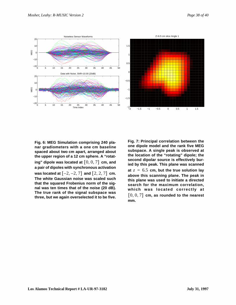
Mosher, Leahy: R-MUSIC Version 2 Page 38 of 40
Los Alamos Technical Report # LA-UR-97-3182 July 31, 1997
0 5 10 15 20 25 30 35 40 45 50−20
−10
0
10
20Noiseless Sensor Waveforms
ME
G
0 5 10 15 20 25 30 35 40 45 50−20
−10
0
10
20Data with Noise, SNR=10.00 (20dB)
Time index
ME
G
Fig. 6: MEG Simulation comprising 240 pla-nar gradiometers with a one cm baselinespaced about two cm apart, arranged aboutthe upper region of a 12 cm sphere. A “rotat-
ing” dipole was located at cm, anda pair of dipoles with synchronous activation
was located at and cm.The white Gaussian noise was scaled suchthat the squared Frobenius norm of the sig-nal was ten times that of the noise (20 dB).The true rank of the signal subspace wasthree, but we again overselected it to be five.
0 0 7, ,[ ]
2– 2– 7, ,[ ] 2 2 7, ,[ ]
−2 −1.5 −1 −0.5 0 0.5 1 1.5−2
−1.5
−1
−0.5
0
0.5
1
1.5
Z=6.5 cm slice Angle 1
Fig. 7: Principal correlation between theone dipole model and the rank five MEGsubspace. A single peak is observed atthe location of the “rotating” dipole; thesecond dipolar source is effectively bur-ied by this peak. This plane was scanned
at cm, but the true solution layabove this scanning plane. The peak inthis plane was used to initiate a directedsearch for the maximum correlation,wh ich was loca ted cor rec t ly a t
cm, as rounded to the nearestmm.
z 6.5=
0 0 7, ,[ ]
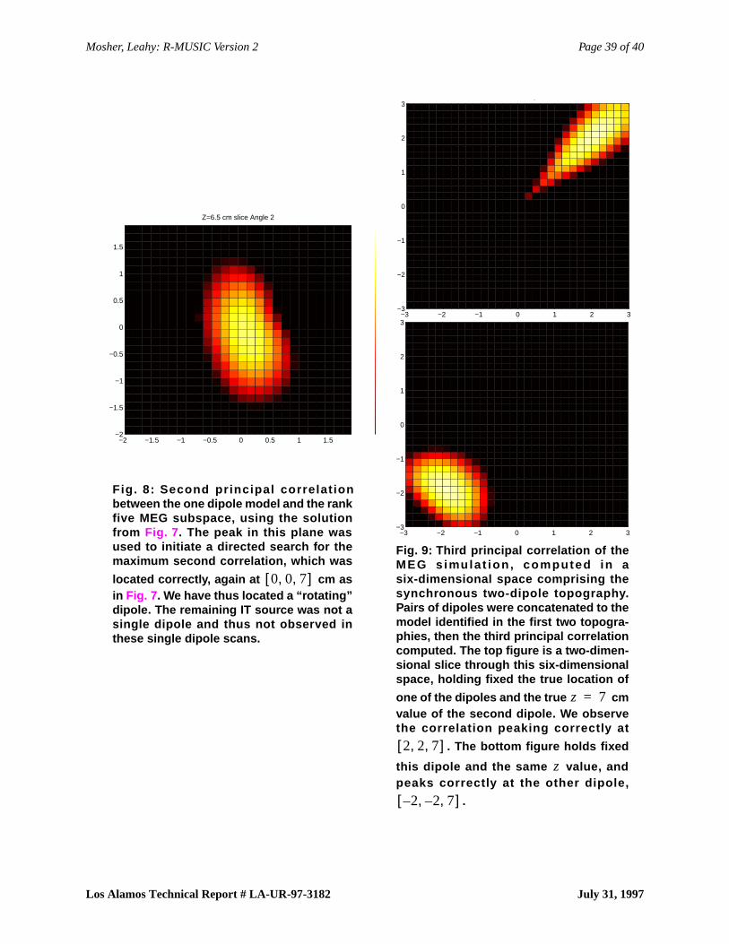
Mosher, Leahy: R-MUSIC Version 2 Page 39 of 40
Los Alamos Technical Report # LA-UR-97-3182 July 31, 1997
−2 −1.5 −1 −0.5 0 0.5 1 1.5−2
−1.5
−1
−0.5
0
0.5
1
1.5
Z=6.5 cm slice Angle 2
Fig. 8: Second pr incipal correlat ionbetween the one dipole model and the rankfive MEG subspace, using the solutionfrom Fig. 7 . The peak in this plane wasused to initiate a directed search for themaximum second correlation, which was
located correctly, again at cm asin Fig. 7. We have thus located a “rotating”dipole. The remaining IT source was not asingle dipole and thus not observed inthese single dipole scans.
0 0 7, ,[ ]
−3 −2 −1 0 1 2 3−3
−2
−1
0
1
2
3Z=7.0, cross slice of Angle 3, 2 dipole−3 −2 −1 0 1 2 3
−3
−2
−1
0
1
2
3g
Fig. 9: Third principal correlation of theMEG s imu la t ion , computed in asix-dimensional space comprising thesynchronous two-dipole topography.Pairs of dipoles were concatenated to themodel identified in the first two topogra-phies, then the third principal correlationcomputed. The top figure is a two-dimen-sional slice through this six-dimensionalspace, holding fixed the true location of
one of the dipoles and the true cmvalue of the second dipole. We observethe correlation peaking correctly at
. The bottom figure holds fixed
this dipole and the same value, andpeaks correctly at the other dipole,
.
z 7=
2 2 7, ,[ ]z
2– 2– 7, ,[ ]
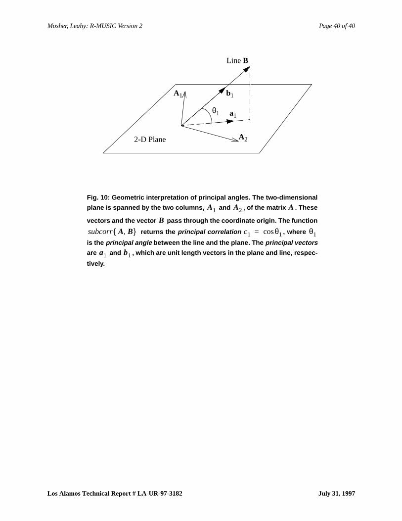
Mosher, Leahy: R-MUSIC Version 2 Page 40 of 40
Los Alamos Technical Report # LA-UR-97-3182 July 31, 1997
2-D Plane
Line B
A1
A2
a1
b1
θ1
Fig. 10: Geometric interpretation of principal angles. The two-dimensional
plane is spanned by the two columns, and , of the matrix . These
vectors and the vector pass through the coordinate origin. The function
returns the principal correlation , where
is the principal angle between the line and the plane. The principal vectors
are and , which are unit length vectors in the plane and line, respec-
tively.
A1 A2 A
BA B,{ }subcorr c1 θ1cos= θ1
a1 b1