Recreation, Tourism, and Rural Well-Being

Recreation, Tourism, and Rural Well-Being/ERR-7Economic Research Service/USDA

United StatesDepartmentof Agriculture

www.ers.usda.gov

A Report from the Economic Research Service

August 2005

Economic

Research

Report

Number 7

Recreation, Tourism,and Rural Well-Being

Richard J. Reeder and Dennis M. Brown

Abstract

The promotion of recreation and tourism has been both praised and criticized as arural development strategy. This study uses regression analysis to assess theeffect of recreation and tourism development on socioeconomic conditions inrural recreation counties. The findings imply that recreation and tourism develop-ment contributes to rural well-being, increasing local employment, wage levels,and income, reducing poverty, and improving education and health. Butrecreation and tourism development is not without drawbacks, including higherhousing costs. Local effects also vary significantly, depending on the type ofrecreation area.

Keywords: recreation, tourism, recreation counties, rural development, economicindicators, social indicators, rural development policy.

Acknowledgments

The authors wish to thank the following reviewers for their helpful comments:Calvin Beale and Pat Sullivan of the Economic Research Service and RickWetherill of Rural Development, all of USDA, as well as Steven Deller of theDepartment of Agricultural and Applied Economics, University of Wisconsin atMadison. Thanks also go to Courtney Knauth for her editing assistance, and toAnne Pearl for the graphic design and text layout of the report.

Contents

Summary . . . . . . . . . . . . . . . . . . . . . . . . . . . . . . . . . . . . . . . . . . . . . . . . . . .iii

Introduction…………………………………… . . . . . . . . . . . . . . . . . . . . .1What Is a Recreation County? . . . . . . . . . . . . . . . . . . . . . . . . . . . . . . . . . .3General Characteristics of Recreation Counties . . . . . . . . . . . . . . . . . . . .3

Economic Impacts . . . . . . . . . . . . . . . . . . . . . . . . . . . . . . . . . . . . . . . . . . . .7Employment . . . . . . . . . . . . . . . . . . . . . . . . . . . . . . . . . . . . . . . . . . . . . . . .8Earnings . . . . . . . . . . . . . . . . . . . . . . . . . . . . . . . . . . . . . . . . . . . . . . . . . . .9Income . . . . . . . . . . . . . . . . . . . . . . . . . . . . . . . . . . . . . . . . . . . . . . . . . . .10Housing Costs . . . . . . . . . . . . . . . . . . . . . . . . . . . . . . . . . . . . . . . . . . . . .12

Social Impacts . . . . . . . . . . . . . . . . . . . . . . . . . . . . . . . . . . . . . . . . . . . . . ..14Population Growth . . . . . . . . . . . . . . . . . . . . . . . . . . . . . . . . . . . . . . . . . .14Travel Time to Work . . . . . . . . . . . . . . . . . . . . . . . . . . . . . . . . . . . . . . . .14Poverty Rate . . . . . . . . . . . . . . . . . . . . . . . . . . . . . . . . . . . . . . . . . . . . . .16

Educational Attainment . . . . . . . . . . . . . . . . . . . . . . . . . . . . . . . . . . . . . .16

Health Measures . . . . . . . . . . . . . . . . . . . . . . . . . . . . . . . . . . . . . . . . . . .17

Crime Rate . . . . . . . . . . . . . . . . . . . . . . . . . . . . . . . . . . . . . . . . . . . . . . . .18

Variations by Type of Recreation County . . . . . . . . . . . . . . . . . . . . . . . .19

Conclusions . . . . . . . . . . . . . . . . . . . . . . . . . . . . . . . . . . . . . . . . . . . . . . . . .24

Ideas for Future Research . . . . . . . . . . . . . . . . . . . . . . . . . . . . . . . . . . . .26

References . . . . . . . . . . . . . . . . . . . . . . . . . . . . . . . . . . . . . . . . . . . . . . . . . .27

Appendix: Regression Analysis . . . . . . . . . . . . . . . . . . . . . . . . . . . . . . . .29

iiRecreation, Tourism, and Rural Well-Being/ERR-7

Economic Research Service/USDA

SummaryWith their high rates of growth, rural recreation counties represent one ofthe main rural success stories of recent years. During the 1990s, theseplaces—whose amenities attract permanent residents as well as seasonalresidents and tourists—averaged 20-percent population growth, about threetimes that of other nonmetropolitan counties, and 24-percent employmentgrowth, more than double the rate of other nonmetro counties. However,tourism- and recreation-based development has been viewed as having nega-tive as well as positive economic and social impacts, leading some localofficials to question recreation development strategies.

What Is the Issue?

Critics argue that the tourism industry—consisting mainly of hotels, restau-rants, and other service-oriented businesses—offers seasonal, unskilled,low-wage jobs that depress local wages and income. As more of a county’sworkforce is employed in these jobs, tourism could increase local povertyand adversely affect the levels of education, health, and other aspects ofcommunity welfare. Meanwhile, the rapid growth associated with this devel-opment could strain the local infrastructure, leading to problems such asroad congestion.

On the other hand, if tourism and recreational development attracts signifi-cant numbers of seasonal and permanent residents, it could change thecommunity for the better. For example, the new residents could spark ahousing boom and demand more goods and services, resulting in a morediversified economy with more high-paying jobs. Even low-paid recreationworkers could benefit if better employment became available. Income levelscould rise, along with levels of education, health, and other measures ofcommunity welfare, and poverty rates could be expected to decline.

This study quantifies the most important socioeconomic impacts of ruraltourism and recreational development.

What Did the Study Find?

Rural tourism and recreational development results in generally improvedsocioeconomic well-being, though significant variations were observed fordifferent types of recreation counties.

Rural tourism and recreational development leads to higher employmentgrowth rates and a higher percentage of working-age residents who areemployed. Earnings and income levels are also positively affected. Althoughthe cost of living is increased by higher housing costs, the increase offsetsonly part of the income advantage.

Rural tourism and recreational development results in lower local povertyrates and improvements in other social conditions, such as local educationalattainment and health (measured by mortality rates). Although rates ofserious crimes are elevated with this kind of development, this may bemisleading because tourists and seasonal residents, while included asvictims in the crime statistics, are not included in the base number of resi-

iiiRecreation, Tourism, and Rural Well-Being/ERR-7


ivRecreation, Tourism, and Rural Well-Being/ERR-7


dents. Rapid growth brings its own challenges, particularly pressures oninfrastructure. The one growth-strain measure examined in the study,commuting time to work, revealed little evidence of traffic congestion inrural recreation areas.

Rural recreation counties have not benefited equally. Rural counties with skiresorts were among the wealthiest, healthiest, and best educated places inthe study, while those with reservoir lakes or those located in the southernAppalachian mountains were among the poorest and least educated. Ruralcasino counties had relatively high rates of employment growth and largeincreases in earnings during the 1990s.

How Was the Study Conducted?

The study assessed the effect of recreation and tourism development on 311rural U.S. counties identified by ERS as dependent on recreation andtourism. The findings here, showing largely positive effects, pertain mainlyto places already dependent on recreational development. Counties justbeginning to build a tourism- and recreation-based economy may not benefitto the same extent.

The authors used multiple regression analysis to determine the degree towhich socioeconomic indicators in the 311 counties had been affected byrecreational development. The key variable in the regression analysis wasrecreation dependency, a composite measure reflecting the percentage oflocal income, employment, and housing directly attributable to tourism andrecreation. For each socioeconomic indicator in the study, two regressionswere computed to explain intercounty variations—one for a single point intime (1999 or 2000) and one for variations in changes that occurred duringthe 1990s. A descriptive analysis, supplementing the regression analysis,compared recreation and other nonmetro county means for each of thesocioeconomic indicators and trends, and then made socioeconomiccomparisons among the different types of rural recreation counties.

1Recreation, Tourism, and Rural Well-Being/ERR-7


IntroductionWhile the economies of many rural areas in the United States have beensluggish in recent years, rural communities that have stressed recreationand tourism have experienced significant growth.1 This has not gone unno-ticed by local officials and development organizations, which have increas-ingly turned to recreation and tourism as a vehicle for development.However, not all observers are convinced that the benefits of this approachare worth the costs. There are concerns about the quality of the jobscreated, rising housing costs, and potential adverse impacts on poverty,crime, and other social conditions.2 This report assesses the validity ofthese concerns by analyzing recent data on a wide range of socioeconomicconditions and trends in U.S. rural recreation areas. The purpose is to gaina better understanding of how recreation and tourism development affectsrural well-being.

Recreation and tourism development has potential advantages and disadvan-tages for rural communities. Among the advantages, recreation and tourismcan add to business growth and profitability. Landowners can benefit fromrising land values. Growth can create jobs for those who are unemployed orunderemployed, and this can help raise some of them out of poverty. Recre-ation and tourism can help diversify an economy, making the economy lesscyclical and less dependent on the ups and downs of one or two industries.It also gives underemployed manufacturing workers and farmers a way tosupplement their incomes and remain in the community. Benefiting fromgrowing tax revenues and growth-induced economies of scale, local govern-ments may be able to improve public services. In addition, local residentsmay gain access to a broader array of private sector goods and services,such as medical care, shopping, and entertainment. While other types ofgrowth can have similar benefits, rural recreation and tourism developmentmay provide greater diversification, and, for many places, it may be easierto achieve than other kinds of development—such as high-tech develop-ment—because it does not require a highly educated workforce.

Many of the potential disadvantages of recreation-related development areassociated with the rapid growth that these counties often experience; onaverage, “recreation counties” grew by 20 percent during the 1990s, nearlythree times as fast as other rural counties. Rapid growth from any cause canerode local natural amenities, for example, by despoiling scenic views.Cultural amenities, such as historic sites, can also be threatened. Growth canlead to pollution and related health problems, higher housing costs, roadcongestion, and more crowded schools, and it may strain the capacity ofpublic services. Small businesses can be threatened by growth-induced “big-box” commercial development, and farms can be burdened by increasedproperty taxes. In addition, newcomers might have different values thanexisting residents, leading to conflicts over land use and public policies.Growth can also erode residents’ sense of place, which might reduce supportfor local institutions, schools, and public services.

Aside from these general growth-related issues, some specific problemshave been linked to tourism and recreation industries. These include thepotential for higher poverty rates associated with low-wage, unskilledworkers who are attracted to the area to work in hotels, restaurants, and

1In this report, “tourism” and“recreation” refer to the developmentprocess in which tourists, seasonal res-idents, and permanent residents areattracted to the community to take partin recreation and leisure activities.

2For a good overall discussion ofthe benefits as well as the liabilities ofrecreation and tourism as a ruraldevelopment strategy, see Gibson(1993), Galston and Baehler (1995),or Marcouiller and Green (2000).



recreation sites. Higher poverty rates could lead to various other social prob-lems, including higher crime rates, lower levels of education, more healthproblems, and higher costs of providing public services.

With this mix of positive and negative impacts, it is understandable whyexperts on development policy may be uncertain about the value of ruraltourism and recreation development strategies. Hence, it is important thatpolicymakers have access to information about the nature and extent of thesocioeconomic impacts of this type of development.

Past research has examined some of the impacts (Brown, 2002). Much ofthat research, however, is in the form of case studies, with only a few empir-ical studies examining nationwide rural impacts, such as the articles byEnglish et al. (2000) and Deller et al. (2001). English et al. examined theimpact of tourism on a variety of measures of local socioeconomic condi-tions (local income, employment, housing, economic structure, and demo-graphic characteristics). Deller and his colleagues examined recreationalamenities (including recreational infrastructure), local government finances,labor supply characteristics, and demographic demand characteristics, esti-mating their effects upon the growth of local population, employment, andincome.

Our research used an approach similar to that of English and his colleagues,which identified a group of tourism-dependent counties and then usedregression analysis to estimate the effect of tourism on various indicators oflocal rural conditions. Using the new ERS typology of rural recreation coun-ties developed by Kenneth Johnson and Calvin Beale (2002), we identifieddifferences between rural recreation counties and other nonmetro countiesfor various indicators of economic and social well-being.3 We also exam-ined socioeconomic variations by type of recreation county. We then usedregression analysis to test statistically for the effect that dependence onrecreation (including tourism and seasonal resident recreation) has on localsocioeconomic conditions. Details about the regression analysis areprovided in the appendix.

We hoped to shed light on several important questions about this develop-ment strategy. Among these are:

� How does rural recreation development affect residents’ ability to find jobs?

� How are local wages and incomes affected?

� How does recreation development affect housing costs and local cost of living?

� What effect does recreation development have on local social problems such as crime, congestion, and poverty?

� How are education and health affected?

� How do various types of recreation areas differ in socioeconomic characteristics?

3We also examined fiscal and eco-nomic conditions in earlier research(Reeder and Brown, 2004), but our fis-cal findings were not easy for us tointerpret, so we excluded them fromthis report.

4We also excluded several countiesthat had been metropolitan in the1980s but had lost their metropolitanstatus by 1993.



What Is a Recreation County?

In 1998, Beale and Johnson identified 285 nonmetropolitan recreation coun-ties based on empirical measures of recreation activity, including levels ofemployment and income in tourism-related industries and the presence ofseasonal housing (Beale and Johnson, 1998). They modified and expandedtheir typology a few years later (Johnson and Beale, 2002). Their 2002typology identified 329 recreation counties that fell into 11 categories,varying by geographic location, natural amenities, and form of recreation. Itis this typology that ERS has adopted as its recreation county typology. Weused the 2002 typology, which covered only nonmetropolitan counties. Tosimplify our analysis, we excluded Alaska and Hawaii.4 This reduced thenumber of recreation counties in our study to 311.

One of the advantages of this typology is that it includes not only placeswith significant tourism-related activity but also those with a significantnumber of seasonal residents. (See box on next page, “How Were Recre-ation Counties Identified?”) Like tourists, most seasonal residents areattracted by opportunities for recreation, including some who come simplyto relax in a scenic rural setting. In theory, seasonal residents should have abigger economic impact on the local community than tourists because theystimulate the housing industry and their season-long presence significantlyincreases the demand for a wide range of local goods and services. In addi-tion, seasonal residents often later become permanent residents. Becausemany seasonal residents first came to the area as tourists, it is difficult, ifnot impossible, to separate the long-term impact of tourists from seasonalresidents. Our use of the ERS typology, which covers both tourism andseasonal recreational/residential development, thus seems ideal for esti-mating the long-term, overall impacts of tourism and recreation combined.

Another advantage of this typology is that it is derived from a continuousvariable—a weighted average of tourism and seasonal housing dependence(see box on next page). In theory, this continuous variable may be usedmore effectively to estimate impacts than a simple recreation/othernonmetro dichotomous variable because it allows us to examine variationsin the extent of recreation. Similarly, the different types of recreation coun-ties in the Johnson/Beale typology can be used to further elucidate and esti-mate the impacts of recreational activity on local socioeconomic conditions.

General Characteristics of Recreation Counties

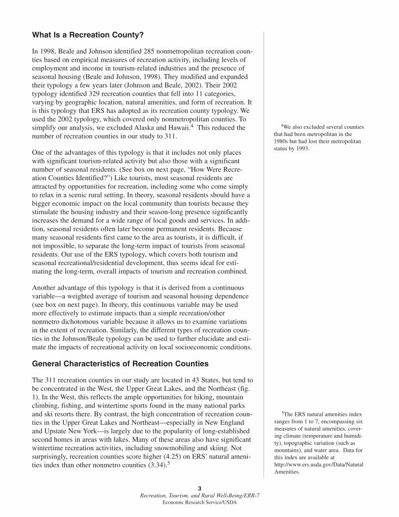
The 311 recreation counties in our study are located in 43 States, but tend tobe concentrated in the West, the Upper Great Lakes, and the Northeast (fig.1). In the West, this reflects the ample opportunities for hiking, mountainclimbing, fishing, and wintertime sports found in the many national parksand ski resorts there. By contrast, the high concentration of recreation coun-ties in the Upper Great Lakes and Northeast—especially in New Englandand Upstate New York—is largely due to the popularity of long-establishedsecond homes in areas with lakes. Many of these areas also have significantwintertime recreation activities, including snowmobiling and skiing. Notsurprisingly, recreation counties score higher (4.25) on ERS’ natural ameni-ties index than other nonmetro counties (3.34).5

5The ERS natural amenities indexranges from 1 to 7, encompassing sixmeasures of natural amenities, cover-ing climate (temperature and humidi-ty), topographic variation (such asmountains), and water area. Data forthis index are available athttp://www.ers.usda.gov/Data/NaturalAmenities.



Data from the 2000 Census reveal that recreation and other nonmetro coun-ties average similar population sizes (table 1).6 However, during the lastdecade, the population of recreation counties has grown almost three timesas fast (20 percent vs. 7 percent, on average). Recreation counties also haverelatively low population densities, and more of their residents tend to livein rural parts of the county (those with less than 2,500 population).

Using the ERS 1993 county economic and policy typologies (Cook andMizer, 1994), we found that the economies in recreational counties weregenerally more diverse than in other nonmetro counties. For example, only30 percent of recreation counties were highly dependent on a single majorindustry (agriculture, mining, or manufacturing), while 58 percent of othernonmetro counties were highly dependent on just one of these industries.Recreation counties also were slightly less dependent on neighboring coun-ties for employment; only 13 percent of recreation counties were identifiedas commuting counties (with a high percentage of their resident workforcecommuting outside the county for employment), compared with 17 percentof other nonmetro counties.

We also found that about a third (32 percent) of recreation counties wereretirement-destination places vs. only 4 percent of other nonmetro counties.

How Were Recreation Counties Identified?

The 2002 Johnson/Beale typology covered only nonmetropolitan counties,

using the 1993 Office of Management and Budget (OMB) definitions of

metropolitan areas. Johnson and Beale began by examining a sample of well-

known recreation areas to determine which economic indicators were most

appropriate for identifying other such counties. They then computed the

percentage share of wage and salary employment from the Census Bureau’s

1999 County Business Patterns data and personal income from Bureau of

Economic Analysis data as these data apply to recreation-related industries,

i.e., entertainment and recreation, accommodations, eating and drinking

places, and real estate. They also computed a third measure: the percentage

share of housing units of seasonal or occasional use, from 2000 Census data.

They then constructed a weighted average of the standardized Z-scores of

these three main indicators (0.3 employment + 0.3 income + 0.4 seasonal

homes). Counties scoring greater than 0.67 on this recreation dependency

measure were considered recreation counties. Next, they added several large

nonmetro counties that did not make the cut but had relatively high hotel and

motel receipts from 1997 Census of Business data. Additional counties were

accepted if the weighted average of the three combined indicators exceeded

the mean and at least 25 percent of the county’s housing was seasonal. Then

Johnson and Beale deleted 14 counties that lacked any known recreational

function but appeared to qualify “either because they were very small in

population with inadequate and misleading County Business Patterns

coverage or because they reflected high travel activity without recreational

purpose, i.e., overnight motel and eating place clusters on major highways.”

These calculations produced their final set of 329 recreation counties. In

2004, ERS established these recreation counties as one of its county typolo-

gies (available at http://www.ers.usda.gov/Briefing/Rurality/Typology/). By

2004, some of these counties had changed their metropolitan status based on

the new 2003 OMB definitions of metropolitan areas.

6The averages shown in this reportare “unweighted” averages (simplemeans). In most cases, these averagesappear to represent fairly the typicalcounty in the group being reported. Insome cases, however, the average(mean) may be unrepresentative in thatit differs significantly from the median.We will point out such instances in thetext or in a footnote.



Note: Excludes counties in Alaska and Hawaii.Source: Adapted from Kenneth M. Johnson and Calvin L. Beale, 2002. “Nonmetro RecreationCounties: Their Identification and Rapid Growth,” Rural America, Vol. 17, No. 4:12-19.

Figure 1

Nonmetropolitian recreation counties, 2002Counties are concentrated in the West, Upper Midwest, and Northeast

Nonmetro recreation countyOther nonmetro county

Metro county

Table 1Demographic characteristics of recreation and othernonmetro counties

Type of county

Indicator Recreation Other nonmetro

Nonmetro counties Numberin our study 311 1,935

PersonsAverage county

population in 2000 26,256 24,138

Population change Percent1990-2000 20.2 6.9

Population density Persons per square milein 2000 35.9 40.2

Rural share of Percentcounty population 79.9 72.4 in 1990

Note: These are county averages (simple means).Source: ERS calculations using data from the U.S. Census Bureau and Bureau of EconomicAnalysis, U.S. Department of Commerce.

Many recreation counties (38 percent) were Federal land counties, meaningthat at least 30 percent of the county’s land was federally owned; only 7percent of other nonmetro counties had that much Federal land. In addition,relatively few recreation counties (10 percent) had experienced persistentlyhigh levels of poverty (from 1950 to 1990), whereas about a fourth (26percent) of other nonmetro counties fell into this category. Because recre-ation counties are not homogeneous with respect to these and other charac-teristics, the averages we present for all recreation counties maskconsiderable variation.



Economic ImpactsThe conventional wisdom among researchers in recent years has been thatrecreation and tourism have both positive and negative economic impactsfor recreation areas.7 On the positive side, recreation development helps todiversify the local economy (Gibson, 1993; Marcouiller and Green, 2000;English et al., 2000), and it generates economic growth (Gibson, 1993;Deller et al., 2001). It achieves this partly by acting as a kind of exportindustry, attracting money from the outside to spend on goods and servicesproduced locally (Gibson, 1993). It also stimulates the local economythrough other means. Infrastructure, such as airports and highways andwater systems, often must be upgraded to meet the needs of tourists, andsuch improvements can help foster the growth of nonrecreation industries inthe area by attracting entrepreneurs and labor and by providing direct inputsto these industries (Gibson, 1993).

Recreation development can involve significant economic leakages,however, in that many of the goods and services it requires come fromoutside the community—for example, temporary foreign workers often aredrawn to the area to fill jobs in hotels, ski resorts, etc.—and many of therecreation-related establishments (restaurants, hotels, tour and travel compa-nies) are owned by national or regional companies that export the profits(Gibson, 1993). Thus, part of the money from tourists and seasonal residentsends up leaving the locality. Another economic drawback involves theseasonality of recreation activities, which can create problems for workersand businesses during off-seasons (Gibson, 1993; Galston and Baehler,1995), though this may actually be a plus for places where seasonal recre-ation jobs are timely, coming when farmers and other workers normallyhave an off-season.

The greatest economic concern is that recreation development may be lessdesirable than traditional forms of rural development because it increasesthe incidence of service employment with relatively low wages. Accordingto Deller et al. (2001), “There is a perception that substituting traditionaljobs in resource-extractive industries and manufacturing with more service-oriented jobs yields inferior earning power, benefits, and advancementpotential” and that this may lead to “higher levels of local underemploy-ment, lower income levels, and generally lower overall economic well-being.” In addition, many researchers are concerned that recreation mayresult in a less equitable distribution of income (Gibson, 1993; Marcouillerand Green, 2000). These problems may be compounded by the higherhousing costs in some recreation areas (Galston and Baehler, 1995).

These concerns reflect findings from individual case studies. Only a fewstudies have attempted to estimate how rural recreation areas nationwidediffer on economic measures. Deller et al. (2001) found that rural tourismand amenity-based development contributed to growth in per capita incomeand employment, and concluded that as a result of the positive impact onincome “the concern expressed about the quality of jobs created … appearsto be misplaced.” English et al. (2000) also found that rural tourism wasassociated with higher per capita incomes, and with a higher percentincrease in per capita income, although they found no significant relation-ship for household income. English and his colleagues also found housing



7Because most economic develop-ment strategies are adopted and imple-mented at the local level, our goalhere is to provide better informeddecisions at that level. Hence, the pos-itives and negatives discussed hererefer only to the situation facing thelocal county. Whether rural recre-ational development is good for theState or the Nation as a whole is alsoa worthwhile question, but beyond thescope of this report.

costs and the change in housing costs over time to be significantly related torural tourism. On the other hand, they found no evidence that the distribu-tion of income was less equal due to rural tourism.

To address these economic issues, we examined a variety of indicatorsreflecting employment, earnings, income, and housing costs.

Employment

Two employment measures, the local employment growth rate (percentincrease during the 1990s) and the local employment-population ratio(percentage of working-age resident population employed in 2000) areparticularly illuminating. (See box “Data Sources” for each of the indicatorsused in this study.)

Recreation counties, on average, had more than double the rate of employ-ment growth of other rural areas during the 1990s: 24 percent vs. 10percent. The regression analysis, moreover, indicated that the extent towhich a recreation county was dependent on recreation was positively andsignificantly related to the rate of local employment growth (see appendixfor details on regression analysis). Employment growth generally offersresidents more job opportunities, enabling some unemployed residents tofind jobs and employed residents to find better jobs. However, job growthdoes not necessarily improve job conditions for current residents. If toomany people come into the area seeking employment, and if thosenewcomers aggressively compete with locally unemployed (or underem-ployed) residents, the resident job seekers may end up having greater diffi-culty gaining employment. Thus, we need to look closely at employmentdata to determine how recreation affects the local ability to find jobs.



Data Sources

The source for most of our data is the Decennial Census (Census Bureau, U.S.

Department of Commerce). Other sources include:

� The Bureau of Economic Analysis, U.S. Department of Commerce, for data on earnings per job, and the Bureau of Labor Statistics, U.S. Department of Labor, Local Area Unemployment Statistics, for employ-ment growth.

� The Uniform Crime Reporting Program (an unpublished data source avail-able on an annual basis from the Federal Bureau of Investigation (FBI)),for data on serious crimes. Note: These data have not been adjusted by the FBI to reflect underreporting, which could affect comparability over time or among geographic areas.

� The Area Resource File (a county-specific health resources information system maintained by Quality Resource Systems, under contract to the Health Resources and Services Administration, U.S. Department of Healthand Human Services), for the age-adjusted death rate, the number of physicians, and the area (in square miles) used to compute population den-sities for regression analysis.

� Kenneth Johnson and Calvin Beale for the recreation county types and the measure of recreation dependency used in their 2002 article.

To measure the ability of residents to find jobs, we examined the percentageof the working-age population that was employed.8 For our study, we brokethis into three separate rates covering three groups of the working-age popu-lation: ages 18-24, 25-64, and 65 and over. We hypothesized that recreationcounties might be particularly advantageous for younger and older popula-tions that may have a harder time competing in places with less job growth.In addition, younger and older groups may find it more convenient to workin recreation counties, which are thought to provide more part-time andseasonal jobs than most other places.

As expected, we found higher employment-population rates in recreationcounties for both the younger and older age groups. However, the differencewas less than 1 percentage point. The main working-age employment rate(ages 25-64) was roughly the same for both recreation and other nonmetrocounties in 2000.9 However, for each of these age groups, the upward trendin the employment-population rate during the 1990s favored recreationcounties. Our regression analysis indicates that recreation had a positive andstatistically significant impact on the employment rates for all three agecategories in 2000. Recreation also had a positive and statistically signifi-cant impact on the increase in the employment rate during the 1990s, exceptfor the older age group.10

Earnings

Conventional wisdom suggests that a main drawback of tourism is thatmany of the jobs it creates are in restaurants, motels, and other businessesthat tend to offer relatively low wages and few fringe benefits. But does thismean that rural recreation development generally leads to low-paying jobs?To address this question, we examined average annual earnings per job(which include wages and salaries and other labor and proprietor income,but exclude unearned income and fringe benefits). We found that averageearnings per job were $22,334 in 2000 for recreation counties—about $450less than in other rural counties (fig. 2, table 2).11 The difference, thoughonly about 2 percent, is consistent with the low-wage hypothesis. On theother hand, our finding that earnings per job increased faster in recreationcounties than in other rural counties in the 1990s was not consistent with theconventional wisdom, but again, the difference was relatively small ($200).

Our regression analysis, however, found no statistically significant relation-ship between earnings per job and recreation dependency, at least no simplelinear relationship.12 With regard to change in earnings per job duringthe 1990s, the regression analysis found that recreation had a positive andstatistically significant impact on earnings per job. So these findings do notsupport the conventional wisdom that recreation results in generally low-paying jobs.

The data on earnings per job covered all jobs in the county, including thosefilled by nonresidents. A different picture emerges when we look only atearnings per resident worker. Aside from excluding nonresidents employedin the county (who, in theory, might be lowering the average earnings perjob in recreation counties), this measure totals the income workers receivefrom all the jobs they have. This is important because recreation countiesoften provide numerous part-time and seasonal jobs, potentially allowing



12When we ran a curvilinear regres-sion, we found a significant negativecoefficient for recreation dependency,and a significant positive coefficientfor recreation dependency squared.This implies that among recreationcounties, those with moderate degreesof recreation dependency had relative-ly lower earnings per job, comparedwith counties with lower or higherrecreation dependencies. We do nothave any explanation for this.

8This may be viewed as a measureof both the availability of job opportu-nities to residents and of local eco-nomic efficiency.

9Comparing medians instead ofmeans, the difference between recre-ation and other nonmetro countiestends to be bigger in 2000 for all threeage groups.

10Our regression explaining thechange in employment rates for theelderly explained only 1 percent of thevariation, which may have preventedthe regression analysis from detectingthe importance of recreation.

11Although the average earnings perjob grew more in recreation countiesthan in other nonmetro counties, thereverse was true for the median earn-ings per job.

more of their residents to have multiple jobs than the residents of othercounties. The average worker’s earnings from multiple jobs exceeded theaverage earnings per job. In recreation counties, earnings amounted to$29,593 per resident worker (16 years or older) in 1999—about $2,000more than in other rural counties—an 8-percent difference.13 Our regres-sion analysis found recreation had a positive and statistically significanteffect on earnings per resident worker. Thus, some residents may work morehours in recreation counties, but on average they end up earning more thanresidents of other nonmetro counties.

Income

Earnings are only one source of income. Other sources include interestreceipts, capital gains, and retirement benefits like social security. Becausemany recreation areas have attracted wealthy individuals—including retirees,whose earnings are only a small part of their incomes—we expected recre-ation county income levels to be higher than in other rural areas. Consistentwith this expectation, we found average per capita income was 10 percenthigher in recreation counties than in other nonmetro counties (fig. 3). More-over, per capita income levels were growing more rapidly during the 1990sin recreation counties than in other nonmetro counties. These findings werereflected in our regression analysis, which found recreation had a positiveand statistically significant effect on both the level of per capita income andthe change in per capita income over time. This should also benefit thecommunity as a whole, because higher incomes mean an increase in demandfor local goods and services, as well as increased local government taxcollections and contributions to local charities and other social organizations.

One problem in interpreting per capita incomes is that they average togetherthe incomes of the wealthiest and the poorest individuals. Thus, a smallnumber of extremely wealthy people could make the community seem much



0

5,000

10,000

15,000

20,000

25,000

30,000

35,000

Earnings per job Earnings per resident worker

Dollars

Figure 2

Earnings in recreation and nonrecreation counties, 1999Recreation counties have significantly higher levels of earnings per resident worker

Source: Calculated by ERS using data from U.S. Census Bureau and Bureau of EconomicAnalysis, U.S. Department of Commerce.

Recreation counties Other nonmetro counties

13Census data also provided medianearnings for two kinds of residentworkers who were 16 years and older:full-time workers and other workers.For both types of workers, recreationcounties surpassed other nonmetrocounties in median earnings per work-er in 2000.

better off than with other measures, for instance, the income of the typical(or median) person in the county. If recreation counties had more wealthyindividuals than other rural counties, the per capita measure might be amisleading indicator of how the average family or household in each ofthese counties differed in income.14 For this reason, we include a secondincome measure: median household income in the county in 1999.

Using this measure, we found that median household income was 10percent higher in recreation counties than in other rural counties. The recre-ation county advantage amounted to $3,185 per year for the median house-hold. The regression analysis reflected this finding, showing a positive and

14In other words, the mean (aver-age) does not equal the median whenincome is not normally distributed.



Table 2Economic conditions in recreation and other nonmetro counties

Type of countyOther

Indicator Recreation nonmetro

Employment growth Percent1990-2000 23.7 9.8

Employment/populationratio in 2000

Ages 16-24 67.4 66.7Ages 25-64 70.3 70.3Ages 65 and over 13.6 13.4

Change 1990-2000 Percentage pointsAges 16-24 0.7 0.0Ages 25-64 0.7 0.3Ages 65 and over 1.5 1.4

Earnings per job Dollarsin 2000 22,334 22,780

Change 1990-2000 5,340 5,140

Earnings per residentworker in 1999 29,593 27,445

Income per capitain 2000 22,810 20,727

Change 1990-2000 7,471 6,564

Median householdincome in 1999 35,001 31,812

Change 1989-1999 11,952 10,531

Median monthly rentin 2000 474 384

Change 1990-2000 134 104

Note: These are county averages (simple means).Source: ERS calculations based on data from U.S. Census Bureau and Bureau of EconomicAnalysis, U.S. Department of Commerce, and Bureau of Labor Statistics, U.S. Departmentof Labor.

statistically significant relationship between recreation and both the leveland change in median family income.

Housing Costs

One of the main complaints about recreation areas is that the cost of livingin them is often higher, offsetting much of the advantage that residentsmight obtain from their higher incomes. Of particular concern is that highliving costs could become a significant hardship for people struggling toraise families on minimum-wage jobs (Galston and Baehler, 1995). A highcost of living could force some lower paid workers (including some long-time residents) to look for housing outside the area.

The cost of housing is one of the most important contributors to the cost ofliving. According to Census data in 2000, median monthly rents for housingaveraged $474 in recreation counties, 23 percent higher than the $384median rent in other nonmetro counties (fig. 4). Our regression analysis alsofound a positive and statistically significant effect of recreation on medianrent. Rents also increased faster during the 1990s in recreation counties,with the extent of recreation positively and significantly related to the extentof rent increase.

Though recreation counties had higher rents than other nonmetro counties,over the course of a year this amounted to a difference of only $1,080 perhousehold—about a third of the $3,185 advantage we found in medianhousehold income in recreation counties. So after deducting for their higherrents, we found that households in recreation counties still had a significantincome advantage over those in other rural counties.15



15Alternatively, we may compareregression coefficients for medianrents and median household incomes.If we multiply the median (monthly)rent coefficient by 12 (months peryear), we get a $384 annual rent add-on associated with a 1-unit increase inrecreation dependency. This compareswith the $1,474 add-on to medianhousehold income associated with thesame 1-unit increase in recreationdependency. Thus, the regressionanalysis implies that higher rentsclaim only about a fourth (26 percent)of the added income related to recre-ation.

0

5,000

10,000

15,000

20,000

25,000

30,000

35,000

2000 1990 to 2000 change


Source: Calculated by ERS using data from U.S. Census Bureau and Bureau of Economic Analysis, Department of Commerce.

Figure 3

Per capita income in recreation and nonrecreation counties, 2000, and change during 1990s Recreation counties have significantly higher levels of income and had moreincome growth in the 1990s

Dollars

It is difficult to draw conclusions from this kind of information, for severalreasons. First, rents show only part of the housing cost picture. Mosthousing units in the nonmetro counties we studied (in both recreation andother nonmetro counties) are owner-occupied rather than rented. Assumingthat higher rents reflect higher home prices and greater equity in homes,higher home prices should increase the wealth of homeowners in recreationcounties. In addition, higher rents and home prices may reflect betterhousing quality in recreation counties, rather than simply higher costs. Thismight be expected because more of the housing in these rapidly growingplaces is likely to be relatively new (and hence more valuable), and recre-ation county residents, having generally higher incomes, may demand betterhousing than residents of other nonmetro counties. Higher home values alsoincrease the local tax base, which may lead to higher tax collections,enabling local governments to increase public services. Thus, on balance, itis unclear whether these higher housing costs are a plus or minus for thecommunity.



Source: Calculated by ERS using data from U.S. Census Bureau, Department of Commerce.

Figure 4

Median monthly rents in recreation and nonrecreation counties, 2000, and change during 1990sRecreation counties have significantly higher rents and had more growth in rents in the 1990s

0

50

100

150

200

250

300

350

400

450

500

2000 1990 to 2000 change

Dollars


Social ImpactsVarious researchers have examined the relationship between nonmetrorecreation and social conditions in a community. Page et al. (2001) note thatrapid population growth in nonmetro recreation counties has resulted inovercrowded conditions and traffic congestion. Recreation may also affectlocal poverty rates. Some authors have argued that recreation activity createsnew sources of employment, helping to raise the poor from poverty (Gibson,1993; Patton, 1985). Others have pointed to the low-wage, seasonal, andpart-time nature of many tourism jobs, arguing that tourism may actuallyadd to the number of poor in the community (Galston and Baehler, 1995;Smith, 1989). Recreation affects social conditions in other ways. Forexample, Page et al. argue that tourism and recreation activity may help tomaintain or improve local services, such as health facilities, entertainment,banking, and public transportation, because of the increased demand thattourists generate for these activities. The relationship between recreation andcrime has also been explored by a number of researchers (Rephann, 1999;Page et al., 2001; McPheters and Stronge, 1974), with a popular questionbeing whether casinos increase criminal activity (Rephann et al., 1997;Hakim and Buck, 1989).

To address social impact concerns, we identified eight social indicators. Twoinvolve conditions associated with rapid population growth; one identifies apopulation subgroup (persons in poverty) that may present special chal-lenges; two relate to education; two deal with health-related concerns; andone measures crime.

Population Growth

The first social variable we examined was the county population growth rateduring the 1990s. Population growth can be beneficial for stagnant ordeclining rural areas looking for new sources of employment and income,but in some places it can bring problems. This is particularly true if growthoccurs rapidly and haphazardly, contributing to sprawl, traffic congestion,environmental degradation, increased housing costs, school overcrowding, adecrease in open land, and loss of a “sense of place” for local residents.

Perhaps because of their natural amenities and tourist attractions, recreationcounties experienced a 20.2-percent rate of population growth between1990-2000, nearly triple the 6.9-percent rate for other nonmetro countiesduring the same period (table 3). These results are consistent with our linearregression analysis, which found a positive and statistically significant rela-tionship between recreation and the county population growth rate. Furtheranalysis revealed an apparent curvilinear relationship, in which recreationcounties with moderate recreation dependencies experienced higher growthrates than those with smaller and larger recreation dependencies.16

Travel Time to Work

This variable was included to test the hypothesis that growth in recreationcounties may lead to increasing traffic congestion (Page et al., 2001). Wefound that mean commute times for recreation and other rural counties werenot significantly different in 2000. Moreover, during the 1990s, commute



16The recreation dependency vari-able had a statistically significantpositive coefficient, while the recre-ation dependency squared variablehad a statistically significant negativecoefficient.

times increased at roughly the same rate (4.4 percent for recreation countiesvs. 4.3 percent for other rural counties). The regression analysis, however,revealed a significant negative relationship between recreation dependenceand change in travel time to work during the 1990s. One explanation maybe that expanded economic opportunities in recreation counties during the1990s meant that residents had to travel shorter distances for jobs.



Table 3Social conditions in nonmetro recreation and other nonmetro counties

Type of county

OtherIndicator Recreation nonmetro

Population growth Percent1990-2000 20.2 6.9

Mean travel time to work Minutesin 2000 22.7 23.0

Change 1990-2000 4.4 4.3

Poverty rate Percentin 1999 13.2 15.7

Percentage pointsChange 1989-1999 -2.6 -3.1

Residents without a Percenthigh school diploma

in 2000 18.4 25.0Percentage points

Change 1990-2000 -7.4 -8.4

Residents with at least Percenta bachelor's degreein 2000 19.2 13.6

Percentage pointsChange 1990-2000 4.0 2.4

Physicians Numberper 100,000 residentsin 2003 123.0 83.4

Age-adjusted deathsper 100,000 residentsin 2003 817.3 898.3

Rate of serious crime Percentper 100 residentsin 1999 2.8 2.4

Note: These are county averages (simple means).Source: ERS calculations based on data from U.S. Bureau of the Census, U.S. Department ofCommerce, Department of Health and Human Services, and the FBI.

Poverty Rate

Poverty poses a problem for communities by increasing the costs ofproviding public services and contributing to crime rates, health problems,and neighborhood blight. Previous research has found that an expandingtourist industry is linked with a decreasing rate of poverty (Rosenfeld et al.,1989; John et al., 1988). Given that many recreation counties have attractedwell-off retirees and that average income levels have risen in recreationcounties, the counties might, on average, be expected to have fewer individ-uals living in poverty than other nonmetro counties. However, as notedearlier, some have argued that tourism, by expanding the number of low-paying, part-time jobs, could increase the number of individuals living inpoverty in these counties (Galston and Baehler, 1995; Smith, 1989).

We found that the poverty rate was substantially lower in recreation countiesthan in other rural counties. In 1999, 13.2 percent of all residents in recre-ation counties were living in poverty, compared with 15.7 percent in othernonmetro counties. Mirroring the national trend of declining poverty ratesduring the 1990s, the proportion of residents living in poverty during thedecade declined (at approximately the same rate) in both recreation andother rural counties.17 Our regression analysis also found a significantlynegative relationship between recreation and the poverty rate.18 In addition,the regression analysis found a statistically significant negative relationshipbetween recreation and the change in the poverty rate.

Educational Attainment

Previous research has identified the central role that education plays inrural poverty (McGranahan, 2000). Education is important, not onlybecause it contributes to the economy, but also because it can affect thequality of life in rural communities and can help raise people out ofpoverty. Nonmetro areas with lower levels of education tend to be poorerand offer fewer economic opportunities for their residents. Migration(movement to another area) tends to increase with higher levels of educa-tion (Basker, 2002; Greenwood, 1993; Greenwood, 1975). Hence, recre-ation counties, which have had many in-migrants in recent years, may beexpected to have higher levels of educational attainment than othernonmetro counties. English et al. (2000) found rural tourism to be associ-ated with higher levels of educational attainment. We examined educationalattainment at two levels: high school and college.

Our results show that residents in recreation counties have higher levels ofeducation than other nonmetro residents (fig. 5). Recreation counties haveboth a smaller share of residents 25 years or older without a high schooleducation, and a higher share of those with at least a bachelor’s degree, thanresidents of other nonmetro counties. In 2000, 18.4 percent of residents age25 or older in recreation counties did not have a high school diploma,compared with 25 percent in other nonmetro counties. For the same year,19.2 percent of recreation county residents age 25 or older had a 4-yearcollege degree or higher, compared with 13.6 percent in other nonmetrocounties. During the 1990s, educational attainment on both measuresimproved in recreation as well as other nonmetro counties. These findings



17Both recreation and other ruralcounties had rates of poverty in 1999higher than the 11.8 percent of metrocounties.

18English et al. (2000) found nosuch relationship.

are supported by our regression analysis, which found that recreation had asignificant negative correlation with the share of residents without a highschool diploma and a significant positive correlation with the share of resi-dents with a bachelor’s degree or higher. In addition, a statistically signifi-cant relationship was found between recreation and an increase in the shareof college-educated residents during the 1990s. However, the change in theshare of high school graduates during the 1990s, although positive, was notsignificantly related to recreation.

Health Measures

Health is important for quality of life. In some recreation counties, manyindividuals moving in are retirees who demand more from health servicesthan younger people; this could result in improved health services in theseplaces. Many recreation counties are in pristine locations with clean air andwater, which might also lead to better overall health. In addition, residentsin recreation areas are probably more likely to be involved in outdoor activi-ties than individuals in other nonmetro areas, which may also promote betteroverall health.

Our indicators of local health conditions—the number of physicians avail-able and the age-adjusted mortality rate—support the view that recreationcounty residents have better health and health services than other nonmetroresidents. In 2003, recreation counties had 123 physicians per 100,000 resi-dents, compared with 83.4 per 100,000 residents in other nonmetro counties.The analysis also shows that the age-adjusted death rate (computed as a 3-year average) was almost 10 percent lower in recreation than in othernonmetro counties.



Figure 5

Educational attainment in recreation and nonrecreation counties, 2000Recreation counties have significantly higher levels of educational attainment

0

5

10

15

20

25

30

No high school diploma Bachelor's degree or higher

Percent

Source: Calculated by ERS using data from U.S. Census Bureau, Department of Commerce.


Our regression results show that recreation had a significantly negativecorrelation with the age-adjusted death rate. However, the relationshipbetween recreation and the number of physicians, although positive, wasstatistically insignificant.

Crime Rate

Many researchers have looked at the link between recreation activity andcrime (Page et al., 2001; Rephann, 1999; McPheters and Stronge, 1974).Some types of recreation counties attract criminals who prey on tourists in-season and rob unoccupied houses during the off-season. Also, some low-income residents of these counties may commit crimes of opportunity,taking advantage of the influx of well-off outsiders. Some researchers haveargued that crime may be particularly associated with casinos (Rephann etal., 1997; Hakim and Buck, 1989).

The results of our analysis indicate that recreation counties had nearly a 17-percent higher rate of serious crime (murder and non-negligentmanslaughter, forcible rape, robbery, and aggravated assault) than othernonmetro counties. In 1999, the overall rate of serious crime in recreationcounties was 2.8 incidents per 100 residents, compared with 2.4 incidentsper 100 residents in other nonmetro counties, a statistically significantdifference. These results are consistent with our regression analysis, whichfound that a significantly positive relationship exists between recreation andthe crime rate.

However, the meaning of this finding is not clear because the crime rate is abiased measure in recreation areas, due to the fact that crimes committedagainst tourists and seasonal residents are included in the total number ofcrimes (the numerator of the crime rate), while tourists and seasonal resi-dents are not included in the base number of residents (the denominator ofthe crime rate). So the crime rate is expected to be higher in recreationareas, even if residents of these areas are not more likely to be crime victimsthan residents of other rural areas.



Variations by Type of Recreation CountyAs noted, Johnson and Beale (2002) categorized each recreation county asbelonging to 1 of 11 mutually exclusive recreational groupings, a classifica-tion that provides greater insight into the recreational component of eachcounty (figs. 6 and 7). The single most common category is the MidwestLake and Second Home, accounting for 70 counties and overwhelminglyconcentrated in central and northern Michigan, Minnesota, and Wisconsin(table 4). The Northeast Mountain, Lake, and Second Home group, a closelyrelated category, is mainly concentrated in northern New England (Maine,New Hampshire, and Vermont) and in portions of New York and Pennsyl-vania. Together, these two similar categories account for more than a quarterof all recreation counties. Both categories are relatively prosperous: North-east counties had the highest level of earnings per job among all recreationtypes, and the Midwest category experienced sharp increases in householdincome during the 1990s (table 5). Both regions had rates of poverty amongthe lowest of all recreation categories (table 6).

Although almost every type of recreation county registered at least double-digit population growth during the 1990s (the exception being the NortheastMountain, Lake, and Second Home), Ski Resort counties grew the fastest(increasing 38 percent), continuing a trend from the 1980s. Other recreationcategories in the West (West Mountain and Other Mountain) also experi-enced rapid population growth. Ski Resort counties stand out in other ways,



Figure 6

Nonmetropolitian recreation categories by type (part 1), 2002


Metro countyNational ParkNE Mtn./Lake/Second HomeMidwest Lake/Second Home

Reservoir LakeCoastal Ocean ResortCasinoOther nonmetro county

measuring substantially higher than other recreation counties on a numberof economic variables, including ratio of employment to population, earn-ings per job, earnings per worker, per capita income, and median householdincome. Ski Resorts also had the lowest poverty rate among all recreationcategories, but had substantially higher housing costs—nearly 40 percenthigher than the average for other nonmetro counties—which grew rapidlyduring the 1990s. Ski Resort counties also stand out in terms of social indi-cators, having the highest levels of educational attainment, the largestnumber of doctors, the lowest death rates, and the highest rate of crimeamong all recreation categories.

In contrast, Reservoir Lake counties and South Appalachian MountainResort counties are among the most economically challenged recreationcounty types. Reservoir Lake counties, which are mainly located in theMidwest and Great Plains regions, and South Appalachian Mountain Resortcounties—in the upland areas of Georgia, North Carolina, Virginia, WestVirginia, and Maryland—have among the lowest earnings per worker andlowest median household income levels. They also have among the lowestrents. Both of these regions have among the lowest levels of educationalattainment. Further, they have higher-than-average age-adjusted death rates,but relatively low crime rates. The South Appalachian Mountain Resortcategory also has a significantly longer commute than other other nonmetrocounties, possibly a reflection of its mountainous topography.



Figure 7

Nonmetropolitian recreation categories by type (part 2), 2002

Metro countyMiscellaneous RecreationSouth Appalachian Mtn. ResortOther Mountain

West MountainSki ResortOther nonmetro county


Casino counties also have relatively low levels of economic development,with the highest rate of poverty—over 40 percent higher than for all recre-ation counties—as well as below-average levels of per capita income,median household income, and earnings per worker. Still, during the 1990s,Casino counties, which are mainly located in the Upper Midwest, theDakotas, the Mississippi Delta region, and Nevada, collectively had sharpemployment growth (a third faster than the average for all recreation coun-ties). Casino counties, which benefited from the establishment of gamblingon Native American reservations during the 1990s, had a lower level ofeducational attainment, fewer physicians, a higher-than-average age-adjusted death rate, and a significantly higher rate of crime than most otherrecreation counties.



Table 4Recreation county categories

Number ofRecreation category counties

Midwest Lake and Second Home 70

Northeast Mountain, Lake, 19and Second Home

Coastal Ocean Resort 35

Reservoir Lake 27

Ski Resort 20

Other Mountain (with Ski Resorts) 17

West Mountain (excluding Ski Resorts 46and National Parks)

South Appalachian Mountain Resort 17

Casino 21

National Park 18

Miscellaneous 21

Total 311

Source: Kenneth M. Johnson and Calvin L. Beale, “Nonmetro Recreation Counties: TheirIdentification and Rapid Growth,” Rural America, Vol. 17, No. 4, 2002:12-19.



Tabl

e 5

Eco

no

mic

co

nd

itio

ns

and

tre

nd

s by

typ

e o

f re

crea

tio

n c

ou

nty

MW

NE

Sou

thN

on-

Oce

anR

eser

voir

Lake

MT

/LK

Nat

.W

est

Ski

Oth

erA

P M

TR

ec.

Rec

.re

c.In

dica

tor

Cas

ino

Res

ort

Lake

Hom

e

Hom

eP

ark

MT

Res

ort

MT

Res

ort

Mis

c.to

tal

tota

l

Em

ploy

men

tP

erce

ntgr

owth

199

0-20

0031

.7*

19.2

*24

.9*

23.3

*3.

519

.0*

25.0

*35

.3*

26.0

*18

.7*

29.2

*23

.7*

9.8

Em

ploy

men

t/pop

ulat

ion

ratio

in 2

000

Age

s 16

-24

66.0

67.5

64.6

67.3

68.8

66.3

66.5

74.3

*67

.266

.168

.167

.466

.7A

ges

25-6

470

.469

.967

.369

.472

.169

.969

.777

.4*

70.6

69.4

71.0

70.3

70.3

Age

s 65

and

ove

r16

.0*

13.8

13.3

10.0

*11

.615

.315

.5*

19.3

*13

.511

.1*

14.8

13.6

13.4

Cha

nge

1990

-200

0P

erce

ntag

e po

ints

Age

s 16

-24

1.0

-1.4

*0.

22.

7*1.

30.

70.

00.

80.

5-0

.1-0

.70.

7*0.

0A

ges

25-6

40.

7-1

.40.

62.

8*1.

10.

5-0

.00.

40.

6-0

.7-0

.40.

7*-0

.3A

ges

65 a

nd o

ver

2.2

1.6

1.2

2.0

0.8

0.9

0.5

3.0

0.8

1.3

0.9

1.5

1.4

Ear

ning

s pe

r jo

bD

olla

rsin

200

0 24

,372

23,6

9819

,630

*22

,710

25,2

55*

21,2

33

20,0

58*

24,2

9423

,560

22,4

1220

,604

22,3

3422

,780

Cha

nge

1990

-200

06,

748

5,76

14,

264

5,35

95,

100

4,38

33,

487*

7,39

4*5,

342

5,84

84,

887

5,34

05,

140

Ear

ning

s pe

r w

orke

rin

199

928

,249

31,9

05*

27,0

3329

,314

*28

,968

*28

,346

28,6

18*

34,9

92*

30,3

91*

28,5

9630

,089

*29

,593

*27

,445

Inco

me

per

capi

tain

200

0

21,8

6526

,628

*20

,002

21,4

8523

,718

*21

,891

20,7

1729

,552

*22

,898

*21

,895

24,2

15*

22,8

10*

20,7

27C

hang

e199

0-20

00

7,45

78,

813*

5,80

2*7,

243*

7,56

6*7,

363

5,70

411

,080

*7,

323

7,83

4*

8,41

9*

7,47

1*6,

564

Med

ian

hous

ehol

din

com

e in

199

933

,325

37,2

39*

29,6

35*

34,8

96*

34,4

47*

33,2

1533

,905

*44

,521

*36

,128

*32

,843

36,3

96*

35,0

01*

31,8

12C

hang

e 19

89-1

999

11,4

7711

,475

*10

,280

13,4

95*

9,41

1*11

,231

11,1

4616

,220

*11

,630

*11

,244

11,6

77*

11,9

52*

10,5

31

Med

ian

mon

thly

ren

tin

200

0 44

0*55

6*

384

421*

460*

445*

47

3*66

0*53

5*43

1*48

8*47

4*38

4C

hang

e 19

90-2

000

115

140*

110

111

85*

126

151*

228*

14

2*12

9*

15

0*

134

104

Not

e:T

hese

are

cou

nty

aver

ages

(si

mpl

e m

eans

).M

W=

Mid

wes

t;N

E=

Nor

thea

st;M

T=

Mou

ntai

n;LK

=La

ke;N

at.=

Nat

iona

l;A

P=

App

alac

hian

;Mis

c.=

Mis

cella

neou

s;R

ec.=

Rec

reat

ion.

*Sig

nific

antly

diff

eren

t fr

om n

onre

crea

tion

coun

ty m

ean

at 5

-per

cent

err

or le

vel.

Sou

rce:

ER

S c

alcu

latio

ns b

ased

on

data

fro

m U

.S.C

ensu

s B

urea

u an

d B

urea

u of

Eco

nom

ic A

naly

sis,

U.S

.Dep

artm

ent

of C

omm

erce

, an

d B

urea

u of

Lab

or S

tatis

tics,

U

.S.D

epar

tmen

t of

Lab

or.R

ecre

atio

n ty

pes

from

Joh

nson

and

Bea

le (

2002

), U

SD

A,

Eco

nom

ic R

esea

rch

Ser

vice

.



Tabl

e 6

So

cial

co

nd

itio

ns

and

tre

nd

s by

typ

e o

f re

crea

tio

n c

ou

nty

MW

NE

Sou

thN

on-

Oce

anR

eser

voir

Lake

MT

/LK

Nat

.W

est

Ski

Oth

erA

P M

TR

ec.

Rec

.re

c.In

dica

tor

Cas

ino

Res

ort

Lake

Hom

e

Hom

eP

ark

MT

Res

ort

MT

Res

ort

Mis

c.to

tal

tota

l

Pop

ulat

ion

grow

thP

erce

nt19

90-2

000

16.7

*18

.8*

20.4

*15

.8*

5.8

13.3

*27

.6*

38.0

*24

.9*

18.4

*23

.3*

20.2

*6.

9

Mea

n tr

avel

tim

e to

wor

kM

inut

esin

200

021

.722

.324

.322

.323

.320

.3*

23.1

22.1

21.2

26.3

*23

.522

.723

.0C

hang

e 19

90-2

000

2.7*

3.8

4.8

4.8*

4.8

4.1

5.1*

4.6

3.9

5.3

3.6

4.4

4.3

Pov

erty

rat

eP

erce

ntin

199

918

.8*

12.4

*15

.210

.7*

12.0

*16

.214

.0*

10.2

*13

.913

.2*

13.3

13.2

*15

.7

Per

cent

age

poin

tsC

hang

e 19

89-1

999

-4.3

-1.6

*-2

.9-4

.4*

0.0*

-4.4

-1.3

*-1

.6*

-1.5

*-2

.6-2

.1-2

.6-3

.1

Res

iden

ts w

ithou

t hi

ghP

erce

ntsc

hool

dip

lom

a in

200

021

.2*

19.0

*23

.618

.0*

18.7

*17

.7*

16.1

*11

.8*

14.5

*24

.719

.8*

18.4

*25

.0P

erce

ntag

e po

ints

Cha

nge

1990

-200

0-7

.3-6

.9*

-9.4

*-8

.9-6

.3*

-6.8

-5.9

*-3

.5*

-5.6

*-1

0.8*

-7.4

-7.4

-8.4

Res

iden

ts w

ith a

t le

ast

Per

cent

a B

.A.d

egre

e in

200

016

.2*

22.5

*13

.314

.9*

17.7

*20

.9*

20.5

*33

.2*

24.3

*17

.0*

19.6

*19

.2*

13.6

Per

cent

age

poin

tsC

hang

e 19

90-2

000

2.7

4.7*

2.8

3.4*

2.7

4.2*

4.5*

6.5*

4.8*

3.4*

4.2*

4.0

2.4

Phy

sici

ans

per

100,

000

Num

ber

resi

dent

s in

200

378

.016

6.6*

52.8

*97

.518

1.9*

110.

110

9.9*

192.

0*19

0.7*

149.

7*11

4.4

123.

0*83

.4

Age

-adj

uste

d de

ath

rate

per

100,

000

resi

dent

s in

200

0-02

955.

683

9.5*

858.

882

9.7*

869.

080

9.1*

766.

3*66

1.7*

759.

3*86

9.7

772.

7*81

7.3*

898.

3

Rat

e of

ser

ious

crim

epe

r 10

0 re

side

nts

in 1

999

3.2*

3.2*

2.0

2.6

2.6

2.5

2.6

3.8*

3.0

2.0

3.3*

2.8*

2.4

Not

e:T

hese

are

cou

nty

aver

ages

(si

mpl

e m

eans

).M

W=

Mid

wes

t;N

E=

Nor

thea

st;M

T=

Mou

ntai

n;LK

=La

ke;N

at.=

Nat

iona

l;A

P=

App

alac

hian

;Mis

c.=

Mis

cella

neou

s;R

ec.=

Rec

reat

ion.

*Sig

nific

antly

diff

eren

t fr

om n

on-r

ecre

atio

n co

unty

mea

n at

5-p

erce

nt e

rror

leve

l.S

ourc

e:E

RS

cal

cula

tions

bas

ed o

n da

ta f

rom

U.S

.Cen

sus

Bur

eau

and

Bur

eau

of E

cono

mic

Ana

lysi

s, U

.S.D

epar

tmen

t of

Com

mer

ce,

and

Bur

eau

of L

abor

Sta

tistic

s,

U.S

.Dep

artm

ent

of L

abor

.Rec

reat

ion

type

s fr

om J

ohns

on a

nd B

eale

(20

02),

US

DA

, E

cono

mic

Res

earc

h S

ervi

ce.

Conclusions This study provides quantitative information on how tourism and recreationdevelopment affects socioeconomic conditions in rural areas. Specifically,we wanted to address economic issues related to employment, income, earn-ings, and cost of living, and social issues such as poverty, education, health,and crime. A summary follows of our main findings on the socioeconomicimpacts of rural recreation and tourism development.

�� Employment. Our regression analysis found a positive and statistical-ly significant association between recreation dependency and the per-centage of working-age population with jobs. We also found that, with the exception of the older (65 and over) population, recreation depend-ency positively affected the change in this employment measure during the 1990s.

�� Earnings. We examined earnings per job and earnings per resident to measure the value of the jobs associated with rural recreation develop-ment. We found that the average earnings per job in recreation countieswere not significantly different than in other nonmetro counties, and we found no direct (linear) relationship between local dependency on recreation and local earnings per job in our recreation counties.However, our regression analysis found a positive relationship between recreation and growth in earnings per job during the 1990s. Thus, the trend seems to favor the pay levels for jobs in these recreation counties.

These findings concern earnings of all who work in the county, includ-ing nonresidents. They report earnings per job, not per worker—an important distinction because workers may have more than one job,and the availability of second jobs (part-time and seasonal) may be greater in recreation counties than elsewhere. When we focused on total job earnings for residents of recreation counties, we found these earnings were significantly higher ($2,000 more per worker) than for residents of other rural counties. The regression analysis also found a significant positive relationship between recreation and resident-workerearnings. So the earnings picture for recreation counties appears posi-tive for the average resident.

�� Cost of living. Our research suggests recreation development leads to higher living costs, at least with respect to housing. We found that the average rent was 23 percent higher in recreation counties, and it was positively and significantly associated with the degree of recreation dependency in our regression analysis. While this may reduce some of the economic advantages for residents of recreation counties, it does soonly partially. Median household incomes, on average, were $3,185 higher in recreation counties than in other rural counties. Annual costs associated with rent were $1,080 higher in recreation counties, offset-ting only about a third of the recreation county income advantage.

�� Growth strains. We found recreation led to significantly higher rates of population growth. In theory, this can aggravate social problems,such as school crowding, housing shortages, pollution, and loss of identification with the community. The one growth-related social prob-lem we addressed was road congestion. Examining the time it takes to commute to work, we found little evidence that congestion was pre-



senting undue problems for residents in recreation counties. Moreover,our regression analysis found that recreation was associated with small-er increases in average commute times in the 1990s than in other rural counties.

�� Poverty. Another social problem that appeared to be reduced in recre-ation counties was poverty. Our regression analysis found recreation was associated with lower poverty rates and with larger declines in the poverty rate during the 1990s.

�� Crime. There may be some cause for concern with regard to crime. We found crime rates (for serious crimes) were higher in recreation counties than in other rural counties, and our regression analysis also found a statistically significant positive relationship between crime rates and recreation dependency. However, crime statistics may be biased in recreation areas because crimes against tourists and seasonal residents are counted in the crime rate, while tourists and seasonal resi-dents are not counted as part of the population base upon which the rate is calculated. Thus, even if people in recreation areas do not face a higher chance of becoming victims of crimes, the crime rates of these areas will appear higher than elsewhere. Nonetheless, one may still argue that recreation-related crime adds to the local cost of policing and incarcerating criminals, just as recreation-related traffic—even though it may not create congestion—adds to the cost of maintaining roads.

�� Education and health. Our analysis found that recreation is associat-ed with a more educated population, particularly with a higher percent-age of college-educated people. We also found relatively good health conditions (measured by age-adjusted death rates) in recreation coun-ties. This might be expected from the higher numbers of physicians per100,000 residents that we found in recreation counties. However, our regression analysis did not find a statistically significant relationship between recreation dependence and the local supply of physicians. So some other explanation must be posited for the general good health in recreation counties, such as greater opportunities for physical exercise or residents who are more health-conscious.

�� Variations by county type. Conditions vary significantly by recre-ation county type. For example, Ski Resort counties have among the wealthiest, best educated, and healthiest populations of all recreation county types. Ski Resort counties also have relatively high rates of crime. In contrast, Reservoir Lake counties and South Appalachian Mountain Resort counties have among the poorest and least educated residents of all recreation county types, along with relatively high age-adjusted death rates, but they have relatively low crime rates. Casino counties—which had among the highest rates of job growth and the largest absolute increases in earnings per job during the 1990s—also had among the highest rates of growth in employment per person for seniors, perhaps reflecting the greater need for jobs among those over age 65 in these relatively high-poverty communities.



Ideas for Future ResearchWe focused mainly on conditions facing residents of mature rural recreationcounties, that is, places that already have a substantial amount of recreation.Additional insights may come from expanding the analysis to includeemerging recreation areas and neighboring places that may be affected byspillover impacts from recreation areas. Future research might also addressissues related to specific population subgroups, such as low-paid workers,who may face more significant problems related to the high cost of housingin recreation areas. The analysis might also be expanded to examine recre-ation impacts on other aspects of community well-being, such as the envi-ronment, public services, institutions like churches and charitablefoundations, and small business formation and entrepreneurial activity.

Our knowledge of rural recreation impacts might also benefit from differentformulations of the regression model. For example, models could be fine-tuned to focus on individual indicators, or they could be estimated sepa-rately for individual regions and types of recreation areas. Feedback effectsmight be incorporated into the model—for example, recreation can lead tohigher housing costs, which in turn can lead to reduced tourism and recre-ation development. More sophisticated models may be able to separate outthese two effects. The models might also be examined over different timeperiods to test for cyclical effects and robustness over time.

Research might also measure the effects of specific State and local policies,along with other factors thought to affect the level of rural recreation andtourism (such as the availability of natural amenities and proximity andaccess to nonmetro areas). This might help State and local officials assesstheir potential for recreation and tourism development and identify strategiesto further this development.



ReferencesBasker, Emek. 2002. Education, Job Search and Migration. WorkingPaper No. WP 02-16, Department of Economics, University of Missouri-Columbia. September.

Beale, Calvin L., and Kenneth M. Johnson. 1998. “The Identification ofRecreational Counties in Nonmetropolitan Areas of the USA,” PopulationResearch and Policy Review, Vol. 17:37-53.

Brown, Dennis M. 2002. “Rural Tourism: An Annotated Bibliography.”Unpublished manuscript, available electronically at:www.nal.usda.gov/ric/ricpubs/rural_tourism.html

Cook, Peggy J., and Karen L. Mizer. 1994. The Revised ERS CountyTypology. RDRR-89, U.S. Department of Agriculture, Economic ResearchService.

Deller, Steven C., Tsung-Hsiu (Sue) Tsai, David W. Marcouiller, andDonald B.K. English. 2001. “The Role of Amenities and Quality of Life inRural Economic Growth,” American Journal of Agricultural Economics,Vol. 83, No. 2, May:352-65.

English, Donald B.K., David W. Marcouiller, and H. Ken Cordell. 2000.“Tourism Dependence in Rural America: Estimates and Effects,” Society &Natural Resources, Vol. 13:185-202.

Galston, William A., and Karen J. Baehler. 1995. Rural Development inthe United States: Connecting Theory, Practice, and Possibilities. Wash-ington, DC: Island Press.

Gibson, Lay James. 1993. “The Potential for Tourism Development inNonmetropolitan Areas,” in David L. Barkley, ed., Economic Adaptation:Alternatives for Nonmetropolitan Areas, pp. 145-64. Boulder, CO: West-view Press.

Greenwood, Michael J. 1975. “Research on Internal Migration in theUnited States: A Survey,” Journal of Economic Literature, Vol. 13, No.2:397-433.

Greenwood, Michael J. 1993. “Migration: A Review,” Regional Studies,Vol. 27, No. 4:295-383.

Hakim, Simon, and Andrew J. Buck. 1989. “Do Casinos Enhance Crime?”Journal of Criminal Justice, Vol. 17:409-16.

John, DeWitt, Sandra S. Batie, and Kim Norris. 1988. A Brighter Futurefor Rural America? Washington, DC: National Governors’ Association,Center for Policy Research.

Johnson, Kenneth M., and Calvin L. Beale. 1994. “The Recent Revival ofWidespread Population Growth in Nonmetropolitan Areas of the UnitedStates,” Rural Sociology, Vol. 59:655-67.



Johnson, Kenneth M., and Calvin L. Beale. 2002. “Nonmetro RecreationCounties: Their Identification and Rapid Growth,” Rural America, Vol. 17,No. 4:12-19.

Marcouiller, David W., and Gary Paul Green. 2000. “Outdoor Recreationand Rural Development.” In Gary E. Machlis and Donald R. Field, eds.,National Parks and Rural Development: Practice and Policy in the UnitedStates, pp. 33-49. Washington, DC: Island Press.

McGranahan, David. 2000. “Boon or Bust? New Technology Manufac-turing in Low-Skill Rural Areas.” U.S. Department of Agriculture,Economic Research Service, Rural Industry briefing room, atwww.ers.usda.gov/Briefing/Industry/boonorbust/ch1.htm.

McPheters, Lee R., and William B. Stronge. 1974. “Crime as an Environ-mental Externality of Tourism: Miami, Florida,” Land Economics, Vol.50:288-92.

Page, Stephen J., Paul Brunt, Graham Busby, and Jo Connell. 2001.Tourism: A Modern Synthesis. London, UK: Thomson Learning.

Patton, Spiro G. 1985. “Tourism and Local Economic Development:Factory Outlets and the Reading SMSA,” Growth and Change, Vol. 16, No.3:64-73.

Reeder, Richard J., and Dennis M. Brown. 2004. “Economic and FiscalConditions in Rural Recreation Counties.” Paper presented before theSouthern Regional Science Association’s annual meeting in New Orleans,LA, March 11-13.

Rephann, Terance J. 1999. “Links Between Rural Development andCrime,” Papers in Regional Science, Vol. 78:365-86.

Rephann, Terance, Margaret Dalton, Anthony Stair, and Andrew Isserman.1997. “Casino Gambling as an Economic Development Strategy,” TourismEconomics, Vol. 3:161-83.

Rosenfeld, Stuart A., Edward M. Berman, and Sarah Rubin. 1989. MakingConnections: ‘After the Factories’ Revisited. Research Triangle Park, NC:Southern Growth Policies Board.

Smith, Michael. 1989. Behind the Glitter: The Impact of Tourism on RuralWomen in the Southeast. Lexington, KY: Southeast Women’s EmploymentCoalition.



Appendix: Regression AnalysisMaking inferences from simple comparisons of recreation and othernonmetro county means can be misleading because it is possible that muchof the observed socioeconomic difference between the two groups could becoincidental and not directly related to the extent of recreation.

For example, during the 1990s, many recreation counties in the RockyMountains benefited from an unusual regional phenomenon associated withthe outflow of population from metropolitan California. This raises a ques-tion: How much of the difference in growth that we observed between recre-ation and other nonmetro counties nationwide was region-specific,associated with this one-time outflow of population?

Similarly, the decade of the 1990s was one of rapid economic improvement,which may have particularly benefited places with high poverty rates,providing job opportunities to many who, under normal conditions, wouldhave had a hard time finding jobs. Many of these high-poverty rural areasare in the South in other nonmetro counties. This largely regional phenom-enon could have led to our finding that recreation counties nationwide bene-fited less from poverty rate reduction than did other nonmetro counties. Butwould we find the same thing if we looked at each region separately?

Other factors unrelated to recreation might also be expected to differentiallyaffect recreation and other nonmetro areas and lead to a potential bias in thedifferences observed between the two types of counties. For example, coun-ties that are more urban in nature may have had developmental advantagesover more rural and isolated areas. While recreation is expected to add tothe level of urbanization, recreation counties are still less urban than othernonmetro counties on average, so this potential bias could mask the benefi-cial impact of recreation in simple comparisons.

Regression Methodology

In an attempt to overcome potential biases, we narrowed our analysis torecreation counties and conducted a regression analysis to see how a recre-ation county’s extent of recreation dependency might affect the socioeco-nomic indicators examined in this report. Our measure of recreationdependency is the weighted average of a county’s Z-scores coveringtourism-related employment and income shares of the local economy andthe recreational home share of total county homes, as developed by Johnsonand Beale (2002): the larger the average, the more dependent a county is onrecreation and tourism.19 In addition, we included 10 dichotomous vari-ables reflecting the Johnson and Beale recreation county types (for statis-tical reasons, we excluded the miscellaneous recreation county type). Thisallows for significant socioeconomic variations by type of recreation county(but it assumes that impacts associated with changes in recreation depend-ency do not vary with recreation type).

Following the approach of English et al. (2000), we also included severalcontrol variables that were not highly correlated with recreation dependencybut that might be expected to affect local socioeconomic conditions. Forexample, we included eight dichotomous (0,1) variables identifying the



19Among the recreation counties weincluded in our analysis, recreationdependency ranged from a minimumof 0.12 to a maximum of 8.60, with amean of 1.56 and a standard deviationof 1.23.

Census regional subdivisions. We did not include a dichotomous variable forone of the nine subdivisions—the Southeast—to avoid statistical problems.

We also included several demographic measures related to urbanization thatare often included in empirical studies explaining regional socioeconomicvariations. One was a dichotomous variable indicating whether the countywas influenced by a nearby metropolitan area (based on adjacency asdefined in the ERS 1993 Beale Codes, which requires both physical adja-cency and significant commuting to the metro area). The other two demo-graphic measures were county population density and percentage of countypopulation residing in the rural portion of the county.

Ideally, an attempt to explain cross-county variations in socioeconomic indi-cators would involve separate models for each indicator, using theory toidentify the explanatory variables and the form of the regression most rele-vant for a particular indicator. Given the large number of indicators in thisstudy, we decided a simpler approach was expedient, so we followedEnglish et al. in using just one set of explanatory variables for all of theindicators examined in our study. This results in some imprecision.

One of the ways our analysis differed from that of English and hiscolleagues was that our regressions only explained variations among our311 recreation counties (rather than including all nonmetro counties asEnglish did). In addition, we ran two ordinary least-squares regressionsexplaining intercounty variations rather than one. One of our regressionsexplained intercounty variations in the year 2000 (or the most recent yearthe data were available). The other regression explained intercounty varia-tions in the change in the indicator over the previous 10 years. The changeregression, which used the identical set of explanatory variables, may beviewed as a check on the year 2000 regression. In most cases, the regres-sions produced similar results: if recreation dependency was significant inthe 2000 regression, it usually had the same sign and was significant in thechange regression.

We also ran additional regressions for each indicator, adding a “squared”version of the recreation dependency variable to allow for a curvilinear rela-tionship. We do not show the results of these additional regressions becausein most cases they did not affect our results—the squared variable eitherexplained little or no additional variation, or it only replaced the non-squared recreation dependency variable in significance with the same sign.In discussing our findings, however, we mention two cases where thesecurvilinear recreation factor regressions provided interesting results.

Regression Findings

Space limitations prevent us from showing the complete regression resultshere, including estimated coefficients for the many control variables weused in our regressions.20 However, we can summarize our findings byshowing only the regression coefficients for the recreation dependency vari-able in the linear regressions we ran to explain variations for each of thesocioeconomic variables of interest. For example, each horizontal row intable 7 summarizes the results of one or two regressions covering a partic-ular socioeconomic variable. Results for the 2000 regression refer to regres-



20Detailed regression results areavailable from the authors uponrequest.

sions that explain socioeconomic variations in the year 2000 (or in the next-closest year available). Results for the 1990s change regression refer toregressions that explain variations in the change in socioeconomic variablesduring the 1990s. Thus, table 7 summarizes the results for 29 regressions.In addition, the regression statistics shown are unstandardized, and oneshould not attempt to draw inferences about their relative importance basedon their magnitudes.

These regression coefficients are generally consistent with what we previ-ously found when comparing simple means for recreation and othernonmetro counties (tables 2 and 3). Dependency on recreation was signifi-cantly related to most of our economic indicators, and the recreationdependency regression coefficients were also generally consistent with mostof our prior findings with regard to social indicators.

In addition, we found statistically significant relationships that were notapparent from comparisons of means for recreation and other nonmetro



Table 7Linear regression analysis measuring the effect of recreation dependency on economic andsocial indicators

2000 regression 1990s change regression

Recreation Regression’s Recreation Regression’sdependency explanatory dependency explanatory

Dependent variables B estimate power1 B estimate power1

Economic indicators:Job growth rate NA NA 5.50** 0.184Employment-populaton ratio:

Ages 16-24 1.13** 0.209 0.56** 0.115Ages 25-64 0.92** 0.211 0.48** 0.139Ages 65 and over 1.04** 0.364 0.30 0.013

Earnings per job -7.95 0.396 482.77** 0.265Earnings per worker2 846.49** 0.317 NA NAIncome per capita 1,044.52** 0.265 487.73** 0.207Median household income2 1,474.40** 0.393 907.59** 0.339Median rent 32.59** 0.516 10.74** 0.377

Social indicators:Population growth rate 4.59** 0.282 2.85** 0.245Travel time to work -0.25 0.327 -0.44** 0.157Poverty rate2 -0.84** 0.249 -0.43** 0.242Percent without HS diploma -1.37** 0.468 0.22 0.341Percent with bachelor’s degree 2.24** 0.491 0.65** 0.211Physicians per 100,000 population3 0.69 0.280 NA NAAge-adjusted death rate

per 100,000 population4 -24.20** 0.290 NA NACrime rate2 0.68** 0.264 NA NA

NA=Not applicable.* The coefficient is statistically different from zero at the .05 level.** The coefficient is statistically different from zero at the .01 level.1Adjusted R-square statistic (fraction of variation explained by regression).2Data are reported for 19993Data are reported for 2003.4Data are reported for 2000-02Source: ERS calculations, based on data from U.S. Census Bureau and Bureau of Economic Analysis, U.S. Department of Commerce, andBureau of Labor Statistics, U.S. Department of Labor.

counties. For example, the regression analysis showed significant positiverelationships between recreation and the employment-population ratios forall three age groups studied, whereas there was little or no difference in themeans for these ratios.

In some cases, the regression analysis raises questions about previouslyobserved statistical differences. For example, we earlier found that recre-ation counties were statistically different from other nonmetro counties withrespect to number of physicians per 100,000 residents, but the regressionanalysis found no statistically significant relationship between this indicatorand recreation dependency.

For travel time to work, we had previously found no statistically significantdifference between recreation and other nonmetro counties, either for theyear 2000 or for the trend during the 1990s. However, the regressionanalysis revealed a statistically significant negative relationship betweenrecreation dependence and change in travel time to work during the 1990s.

One of the more interesting findings was recreation dependency’s negativeand statistically significant relationship with the change in poverty rate.This means that the more recreation dependent a county is, the bigger itsdecline in poverty rate during the 1990s, controlling for other factors. Thefinding contrasts with our simple descriptive analysis, which found thatrecreation counties had, on average, a smaller decline in poverty than othernonmetro counties during the 1990s. This suggests that, as we suspected,the smaller average decline in poverty for recreation counties may havebeen simply a geographic coincidence, because when we controlled forregional differences and other factors in our regression analysis we foundthat the higher a county’s recreation dependency, the more its poverty wasreduced during this decade.

Another interesting finding involved earnings per job. We initially found thatrecreation dependency had a negative but statistically insignificant coefficientfor earnings per job (in the 2000 model). When we ran the curvilinearversion of the first regression (the 2000 model), we found a significant nega-tive coefficient for recreation dependency and a significant positive coeffi-cient for recreation dependency squared.21 This implies that the recreationcounties with moderate degrees of recreation dependency had relativelylower earnings per job, while those with higher or lower recreation depend-ency had higher earnings. Taken together, these findings present a somewhatmuddled picture with respect to recreation impacts on earnings per job—there is no clear indication that recreation hurts a county in this regard. Wegot a clearer regression finding regarding the change in earnings per jobduring the 1990s, which revealed a positive and significant relationshipbetween recreation dependency and the growth in earnings per job.

Two other indicators had different results for the 2000 regressions and the1990s change regression: the employment population ratio for the elderlyand the percent of adult (ages 25 and older) residents without high schooldiplomas. In both cases, the regressions explaining the change in the indi-cator produced insignificant coefficients for recreation dependency. For theemployment-population ratio for ages 65 and up, the change regressionperformed very poorly, explaining less than 6 percent of the variation—less



21The nonlinear version of thechange regression did not produce asimilar significant relationship.

than any other regression in our analysis. This suggests that we might finda significant relationship if we were to improve the model to explain thebehavior of the elderly. For the other indicator, the percentage without highschool diplomas, we may need to find some other explanation, since theregression explaining change for this indicator performed better in terms ofexplaining variation than all of our other change-form regressions. Perhapssomething unusual was going on in the 1990s that kept places with higherrecreation dependencies from experiencing more significant declines in thepercentage lacking high school degrees.22

We have already mentioned recreation’s curvilinear relationship with earn-ings per job. The other case where we found a curvilinear relationshipinvolved recreation’s effects on population growth rates in the 1990s. Thelinear regression explaining population growth rate had a statistically signif-icant positive coefficient for recreation dependency. The curvilinear regres-sion had a statistically significant positive coefficient for recreationdependency and a statistically significant negative coefficient for recreationdependency squared. This implies that counties with moderate recreationdependencies have higher growth rates than counties with smaller or largerrecreation dependencies.



22For example, it may be that dur-ing the 1990s, higher educated retireesbegan to move to a wider array ofrecreation areas, whereas before theymay have concentrated in the mostrecreation-dependent areas.

Recreation, Tourism, and Rural Well-Being

Documents

Transcript of Recreation, Tourism, and Rural Well-Being