April 8, 2009

Recovery Before Redemption:A Theory of Delays in Sovereign Debt Renegotiations

David Benjamin∗

State University of New York, Buffalo

Mark L. J. Wright∗

University of California, Los Angeles

ABSTRACT

Negotiations to restructure sovereign debts are protracted, taking on average almost 8 years tocomplete. In this paper we construct a new database (the most extensive of its kind covering ninetyrecent sovereign defaults) and use it to document that these negotiations are also ineffective in bothrepaying creditors and reducing the debt burden countries face. Specifically, we find that creditorlosses average roughly 40 per-cent, and that the average debtor exits default more highly indebtedthan when they entered default. To explain this apparent large inefficiency in negotiations, wepresent a theory of sovereign debt renegotiation in which delay arises from the same commitmentproblems that lead to default in the first place. A debt restructuring generates surplus for the partiesat both the time of settlement and in the future. However, a creditor’s ability to share in the futuresurplus is limited by the risk that the debtor will default on the settlement agreement. Hence, thedebtor and creditor find it privately optimal to delay restructuring until future default risk is low,even though delay means some gains from trade remain unexploited. We show that a quantitativeversion of our theory can account for a number of stylized facts about sovereign default, as well asthe new facts about debt restructurings that we document in this paper. Finally, we argue that ourfindings shed light on the existence of delays in bargaining in a wider range of contexts.

∗We thank Lee Ohanian, Christoph Trebesch, Vivian Yue, numerous seminar participants, as well as partic-ipants at the 2007 Society for Economic Dynamics meetings in Prague, for comments. Further commentswelcome. Benjamin: db64@buffalo.edu. Wright: mlwright@econ.ucla.edu.

1 Introduction

In many economic environments, agents appear to have trouble reaching mutually

advantageous agreements. In this paper, we document that this phenomenon is especially

severe in the case of debt restructuring negotiations between a sovereign country in default and

its international creditors. Using a new database of sovereign debt restructuring outcomes,

the most extensive of its kind covering ninety recent sovereign defaults, we show that the

average default takes more than 7 years to resolve, results in creditor losses (or “haircuts”)

of roughly 40 per-cent, and leaves the sovereign country more highly indebted than when

they entered default. To explain this apparent inefficiency, we present a theory of sovereign

borrowing, default, and debt restructuring in which delays in debt restructuring are the

result of the same commitment problems that lead to default in the first place. As a debt

restructuring agreement produces gains for the debtor country both in the period of the

settlement, and in the future, the country would like to promise a share of these future gains

as part of a settlement. However, there is a risk that the country will default on such a

promise. As a result, both the country and its creditors find it privately optimal to delay

restructuring until future default risk is low. We show that a quantitative version of the

theory can account for a number of stylized facts about sovereign default, as well as the

new facts on debt restructurings that we document in this paper. Finally, we use the theory

to examine the efficacy of bailouts by multilateral institutions as a tool for both providing

insurance to debtor countries, and for encouraging a prompt restructuring.

We begin by presenting our database of sovereign debt restructuring outcomes. Drawn

from a variety of sources, the database covers 90 defaults by 73 countries that were settled

during the period 1989 to 2006, and contains data on the occurrence of default and settlement,

the outcomes of negotiations, as well as measures of economic performance and indebtedness.

In addition to the three facts introduced above, we emphasize three facts about the relation-

ship of these outcomes to economic activity, and to each other, that motivate the development

of our theory below. Specifically, we find that longer defaults are correlated with larger hair-

cuts, and that there is a modest (but only a modest) tendency for countries to enter default

when output is relatively low, and to emerge from default once output has recovered to its

trend. Finally, we also establish that longer defaults and larger haircuts are more likely when

economic conditions in the defaulting country are weak at the time of default.

We then present our theory of sovereign borrowing, default and debt restructuring.

In the theory, international debt markets are incomplete so that default offers the sovereign

country partial (and costly) insurance against adverse economic outcomes. While in default,

and until it has settled with its creditors, output in the country is reduced, and access to

international financial markets is limited. As a result, surplus is wasted while the country is

in default, and the country and its creditors bargain over shares of this surplus. Bargaining

takes place under complete information, with the bargaining power of the parties fluctuating

over time. A settlement consists of a transfer of current resources as well as a new debt issue

which serves to share the future surplus generated by a settlement. The value of a settlement

to creditors, therefore, depends on the market value of the new debt issue, which is in turn

limited by the fact that the country may default on these debts. Delay arises as both the

country and creditor find it optimal to wait until the value of any debt issued as part of a

settlement has recovered before agreeing on a settlement and redeeming the old debts.

We next take the theory to the data and show that it is capable of matching the

new debt restructuring facts above, as well as a number of facts about sovereign borrowing

and default stressed in previous studies. Calibrating bargaining power in our model to the

relationship between default and economic activity in the data, we generate some defaults

when output is high as a result of a favorable bargaining position for the debtor. Other

defaults occur following a sequence of low income levels. In such cases, the possibility of a

settlement leads creditors to lend even when default risk is high, supporting higher levels of

borrowing (at face value) at higher interest rates than in previous models. Defaults occur

when the ability to raise debt levels in response to another negative income shock is limited.

When debt levels are high, settlements consist largely of new debt issues, and occur only after

significant improvements in economic circumstances or bargaining conditions that raise the

value of new debt issues. This is the source of delay in our model. Likewise, when the face

value of the defaulted debt is high we get large haircuts, generating a positive correlation

between delay and haircuts. Since countries exit default when circumstances have improved,

they are able to borrow more than they could just prior to default. Thus, debt levels often

rise upon exit from default. The volatility of sovereign spreads is increased by both volatility

2

in the size of the expected settlement, and the greater variability in debt levels.

Our paper contributes to a number of literatures. We believe we are the first to charac-

terize the empirical relationship between delay, haircuts and debt levels for sovereign countries

in default, while our characterization of creditor losses for ninety defaults triples the number

of estimates previously available (e.g. Cline 1995 and Sturzenegger and Zettelmeyer 2007).

Our theory contributes to the recent literature on debt and default in both an international

(Arellano 2007, Kovrijnykh and Szentes 2007, Yue 2007, and Mendoza and Yue 2008) and do-

mestic (Chatterjee et al 2007) context. Unlike all of these papers, our theory generates delays

in bargaining, and does so without appealing to collective action problems among creditors

(unlike Pitchford and Wright 2007, 2008), and while simultaneously explaining the evolution

of debt during the default restructuring process (unlike Bi 2008 and d’Erasmo 2008). Finally,

we view our work as a contribution to the broader literature on delays in bargaining. Our

finding that delays are predictable leads us to focus on commitment problems with complete

information, and abstract from the role of asymmetric information (unlike the work surveyed

by Ausubel, Cramton, and Deneckere 2002). Our approach extends the abstract bargaining

environment of Merlo and Wilson (1995) by allowing for outside options, flow payoffs, and

an endogenous terminal payoff.

The rest of this paper is organized as follows. Section 2 describes our database of

sovereign debt restructuring outcomes and presents our empirical findings. Section 3 presents

our theory, first analyzing the debt restructuring process taking borrowing outcomes as given,

before analyzing borrowing outcomes taking the debt restructuring process as given. We then

combine the restructuring environment with the borrowing environment and provide a proof

of existence of an equilibrium for the overall model. Section 4 shows that a calibrated version

of the model can match the facts introduced in Section 2, while Section 5 evaluates the effect

of supranational bailout policies. Section 6 concludes by reinterpreting the phenomenon

of worldwide sovereign debt crises in the light of our results, and considering the theories

implications for negotiations in other contexts. An appendix collects tables and figures,

proofs of theorems, and provides further details on our database.

3

2 Sovereign Debt Restructuring Facts

In this section we describe our database of sovereign defaults and debt renegotiation

outcomes, and present our empirical findings.

2.A Data Sources and Construction

In setting the limits of our database, we restrict attention to defaults on sovereign debts

owed to private sector creditors, like banks and bondholders. The reason is that, in our model

of debt restructuring below, creditors bargain with a view to maximizing the value of their

settlement, while official creditors like the International Monetary Fund and creditor country

governments are arguably motivated by broader concerns of equity. We define sovereign debts

to include debts owed either directly by a country’s national government, or owed indirectly

by virtue of a government guarantee. The most comprehensive and widely used source of

data on the dates of defaults on sovereign debts owed to private sector creditors, as well as the

dates of settlements of these defaults, is published by the ratings agency Standard and Poors

(Beers and Chambers 2006). Standard and Poors (S&P) defines a default on a debt contract

to have occurred if a payment is not made within any grace period specified in the contract,

or if debts are rescheduled on terms less favorable than those specified in the original debt

contract. S&P defines the end of a default as occurring when a settlement occurs, typically

in the form of an exchange of new debt for old debt, and when they conclude that “no further

near-term resolution of creditors claims is likely” (page 22). Defining a default to have begun

when debts are rescheduled on unfavorable terms, which is also related to the definition of

a settlement, may result in an underestimate of actual delays in bargaining. Standard and

Poors record only the year in which a default started and ended, and so we supplement these

dates with data from Arteta and Hale (2007), Pitchford and Wright (2007) and Trebesch

(2008), as well as a range of primary sources, to come up with the month, and in some cases

the day, in which a default started and ended.

The most novel part of our dataset lies in its estimates of creditor losses, or haircuts,

for a large number of defaults. Until now, there has existed only a small number of estimates

produced by different researchers using different methods for largely non-overlapping sam-

4

ples of defaults1. In order to obtain the largest sample possible, and to ensure consistency of

treatment, we base our measures on the World Bank’s estimates of debt stock reduction, in-

terest and principal forgiven, and debt buybacks, as published in Global Development Finance

(GDF). We combine the World Bank’s estimates of the reduction in the face value of the debt

with estimates of the forgiveness of arrears on interest and principle. As the World Bank data

do not make any distinction between forgiveness of debts by private creditors and forgiveness

by official creditors, we scale the amount of forgiveness using estimates of the total amount

of debt renegotiated, and on the proportion owed to private creditors, from both GDF and

Institute for International Finance (2001). Losses in different years were added together and

discounted back to the time of the default using a ten per-cent discount rate, following the

practice of the OECD Development Assistance Committee and the World Bank (Dikhanov

2006). As shown in Appendix C, our estimates correlate closely with those of other studies.

The resulting series on private creditor haircuts covers ninety defaults and renego-

tiations by seventy-three separate countries that were completed after GDF data on debt

forgiveness first became available in 1989 and that ended prior to 2006. Our data on default

dates and haircuts were then combined with data on various indicators of economic activity

taken from the World Bank’s World Development Indicators publication, and with data on

the stock of long term sovereign debt outstanding from GDF. Short term debt is not included

because it is not available disaggregated by type of creditor.

2.B The Facts

Table 1 presents some summary statistics on the length of time taken to settle a default,

which we refer to as delay, and on average haircuts weighted by the level of outstanding debt.

There are three instances of defaults being contiguous in time, in the sense that S&P dates a

default by a country as ending in the same year, or year before, another default begins2. We

present results treating these defaults both as separate events (“delay 1”), and treating them

1We have uncovered estimates of haircuts in 27 defaults, constructed by four different authors using fivedifferent methods. All of the estimates are tabulated for the purposes of comparison in Appendix C.

2The three episodes are: Ecuador, who S&P treat as being in default from 1999 to 2000, and again from2000 to 2001; Russia, in default from 1991 to 1997, and from 1998 to 2000; and Venezuela, in default from1995 to 1997, and in 1998.

5

as a single default episode (“delay 2”). Treating contiguous defaults as distinct defaults, there

are ninety defaults in our sample lasting an average of 7.4 years. Delays rise to an average of

7.6 years if contiguous defaults are treated as a single default event. In our sample, delay is

slightly higher than found in other studies, such as Pitchford and Wright (2008), who record

an average delay of 6.5 years for a larger sample of defaults in the modern era. This leads

to our first result:

Fact 1: sovereign defaults are time consuming to resolve, taking almost eight years on average

in our sample.

Table 1 also presents evidence on the average size of haircuts, where the average is

weighted by the value of outstanding debts for the case of contiguous defaults. As shown in

the Table, the average creditor experienced a haircut of roughly 40 per-cent of the value of the

debt. Further information on the sizes of haircuts and delays is presented in Figure 1 which

contains a scatter plot of haircuts and delays for each of the ninety settlements contained in

our sample. As shown in the Figure, haircuts in our sample have ranged from approximately

zero all the way up to ninety per-cent of the value of creditors claims in the case of some

African defaults. Likewise, there is a great deal of variation in delays with many defaults

being settled almost immediately while others are settled in excess of two decades. There

is also a noticeable positive relationship between the amount of delay in renegotiation and

the size of the haircut, with the correlation coefficient between the two series equalling 0.66.

This gives rise to our next two results:

Fact 2: creditor losses (or haircuts) are substantial, with the average creditor experiencing

a reduction in the value of their claim of forty-four per-cent.

Fact 3: longer defaults are associated with larger haircuts, with a correlation between the

length of the renegotiation process and the size of the creditor haircut of two-thirds.

One possible explanation for Fact 3 is that there is a common factor driving both

longer defaults and larger haircuts. To examine this, Table 1 also presents evidence on the

relationship between delays and haircuts and the level of economic activity in the year of the

default. In particular, the third column shows that the larger is the decline in output in the

6

year of default, the longer the delay and the larger the haircut, on average. The relationship

is only modest, however, never rising above 0.3 in absolute value, with the correlation to

haircuts barely different from zero. The fourth column Table 1 presents the relationship

between delays and haircuts and the growth of output in the two years surrounding the

default and finds a stronger negative relationship with haircuts. This leads to our fourth

fact:

Fact 4: larger output declines in the year of default are associated with modestly longer

defaults and larger haircuts, with correlation coefficients around −0.25

Table 2 provides further evidence on the relationship between defaults, settlements and

output. As shown in the first column, there is a broad tendency for default to be associated

with adverse economic conditions, with a mean level of output roughly one-half of one per-

cent below trend3, while output in non-default periods is above trend by an equal amount on

average. Economic adversity is particularly likely in the first year of a default, when output

was on average 1.3 per-cent below trend, and tends to have dissipated by the time a country

settles with its creditors when output is on average only 0.2% below trend. Nonetheless,

there is a great deal of variation across country experiences so that the overall relationship

between output and default is quite weak. In almost one-third of cases, a country defaults

with output above trend. This confirms the earlier finding of Tomz and Wright (2007) for a

larger sample of defaults, and leads to our fifth result:

Fact 5: defaults are somewhat more likely to occur when output is below trend, and settle-

ments tend to occur when output has returned to trend, with 64% of defaults beginning when

output is below trend, and 49% ending when output is above trend. The average deviation

of output from trend is −1.3% in the first year of a default, and −0.2% in the year of the

settlement.

Table 2 also explores the relationship between defaults and debt levels for the default-

ing country. As shown in the table, being in default is associated with levels of debt to GDP

3Deviations from trend are calculated using a Hodrick-Prescott filter with smoothing parameter 6.25 forannual data (see the discussion in Ravn and Uhlig 2002). Tomz and Wright (2007) establish that these factsare robust to different filtering methods.

7

that are more than seventy per-cent higher than for when a country is not in default, bearing

in mind that our sample of countries is conditioned upon having defaulted once during this

period. Strikingly, the table reveals that the average country exits default with levels of

debt that are 25 per-cent higher than they possessed when they entered default. This figure

is accentuated by some outlier countries, but even the median country exits default with 5

per-cent more debt. From this we conclude that renegotiations are ineffective at reducing the

indebtedness of a debtor country. This leads to our sixth result:

Fact 6: default resolution is not associated with decreased country indebtedness, with the

median and average country exiting default with a debt to GDP ratio 5 and 25 per-cent

higher than before they entered default, respectively.

Finally, Table 1 also shows that delays and haircuts are essentially unrelated to the initial level

of indebtedness of a country. In our theory, which we begin to outline in the next section,

we therefore do not focus upon differences in debt levels as a major factor in negotiations.

3 A Theory of Sovereign Debt, Default, and Debt Restructuring

In this section, we present our theory of sovereign borrowing and default. We begin

by first describing the decisions facing a sovereign country that is in good standing with its

creditors, before moving on to a description of international credit markets, and then to the

debt restructuring environment, devoting the most detail to the latter.

3.A The Borrowing and Default Environment

The Sovereign Borrower

Consider a world in which time is discrete and lasts forever. In each period t = 0, 1, ..,

a sovereign country receives an endowment of the single non-storable consumption good e (s)

that is a function of the exogenous state s which takes on values in the finite set S. Thus,

the endowment also takes on only a finite number, Ne, of values. The state s summarizes

all sources of uncertainty in the model and evolves according to a first order Markov process

with transition probabilities given by a transition matrix with representative element π (s′|s).

Below, the evolution of the state s will also govern the evolution of the country’s bargaining

position with creditors.

8

The sovereign country is represented by an agent that maximizes the discounted ex-

pected value of its utility from consuming state contingent sequences of the single consumption

good {ct (st)} according to∞∑

t=0

βt∑st|s0

π(st|s0

)u(ct

(st))

.

Here, the felicity function u is twice continuously differentiable, strictly increasing and strictly

concave so that the country is averse to fluctuations in its consumption. The notation st|s0 is

used to denote a history of the state that begins with state s0, while π (st|s0) is the product of

the associated one-period ahead conditional probabilities. The discount factor β lies between

zero and one and is assumed to imply a discount rate in excess of the world interest rate. As

a result, international borrowing may be motivated by both a desire to smooth consumption,

as well as a desire to tilt a country’s consumption profile forward in time.

A sovereign country that is not in default enters a period with a new value of the state

s, and a level of international debt b. It is assumed that b must lie in the set of debt levels,

B, which is finite with cardinality Nb, and contains both negative and positive elements, as

well as the zero element, where negative elements are interpreted as savings by the country.

We let V (b, s) denote the value function of a country of that enters the period with debt b

and state s, before the country has decided whether or not to default, which is an Ne by Nb

vector of real numbers.

The sovereign’s first decision is whether or not to default on its debts. If the sovereign

defaults, they receive a payoff given by V D (b, s) , which is a Ne by Nb vector of real numbers,

and which will be determined below when we describe the process by which a country in

default bargains with its creditors. If we let V R (b, s) denote the value function of a country

that enters the period with debt b and state s, after it has decided to repay it’s debts, which

is an Ne by Nb vector of real numbers, then the value function V (b, s) satisfies

V (b, s) = max{

V R (b, s) , V D (b, s)}

. (1)

If the sovereign country repays its debts, it must decide how much to consume c and

how much debt b′ ∈ B to take into the next period. The value function associated with the

9

repayment of debt, V R, is defined by

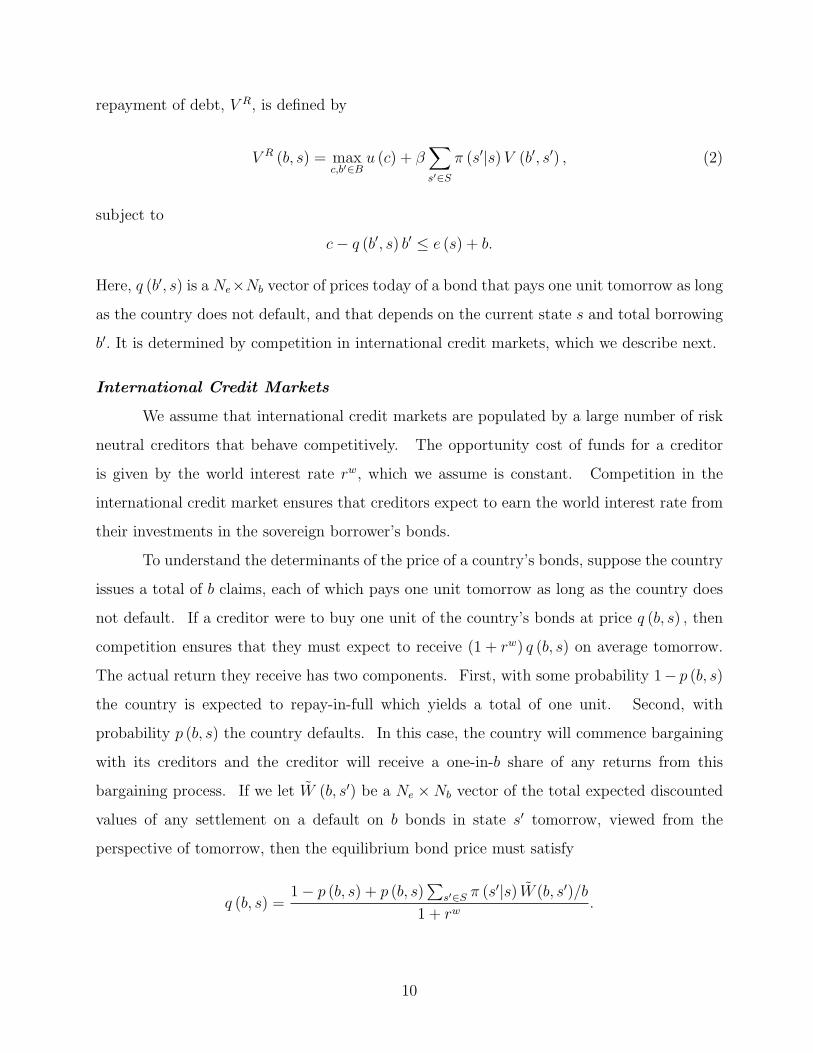
V R (b, s) = maxc,b′∈B

u (c) + β∑s′∈S

π (s′|s) V (b′, s′) , (2)

subject to

c− q (b′, s) b′ ≤ e (s) + b.

Here, q (b′, s) is a Ne×Nb vector of prices today of a bond that pays one unit tomorrow as long

as the country does not default, and that depends on the current state s and total borrowing

b′. It is determined by competition in international credit markets, which we describe next.

International Credit Markets

We assume that international credit markets are populated by a large number of risk

neutral creditors that behave competitively. The opportunity cost of funds for a creditor

is given by the world interest rate rw, which we assume is constant. Competition in the

international credit market ensures that creditors expect to earn the world interest rate from

their investments in the sovereign borrower’s bonds.

To understand the determinants of the price of a country’s bonds, suppose the country

issues a total of b claims, each of which pays one unit tomorrow as long as the country does

not default. If a creditor were to buy one unit of the country’s bonds at price q (b, s) , then

competition ensures that they must expect to receive (1 + rw) q (b, s) on average tomorrow.

The actual return they receive has two components. First, with some probability 1− p (b, s)

the country is expected to repay-in-full which yields a total of one unit. Second, with

probability p (b, s) the country defaults. In this case, the country will commence bargaining

with its creditors and the creditor will receive a one-in-b share of any returns from this

bargaining process. If we let W (b, s′) be a Ne ×Nb vector of the total expected discounted

values of any settlement on a default on b bonds in state s′ tomorrow, viewed from the

perspective of tomorrow, then the equilibrium bond price must satisfy

q (b, s) =1− p (b, s) + p (b, s)

∑s′∈S π (s′|s) W (b, s′)/b

1 + rw.

10

The total expected discounted value of any settlement, viewed from tomorrow, W (b, s′)

will be determined along with the Ne × Nb vector of values to the country from default

V D (b, s) , as a result of the bargaining process which we describe in the next section. For

now, we assume that W (b, s′) is bounded below by zero and above by b, which in turn ensures

that the bond price function takes values in the interval [0, 1/ (1 + rw)] ; we prove that W has

these properties below. We let Q (B × S) be the set of all functions on B × S taking values

in [0, 1/ (1 + rw)] .

It remains to describe the probability of default p (b, s) , which is determined by the

sovereign’s decision to default described in (1) above. For most values of (b, s) , the sovereign

country will strictly prefer defaulting over repaying, or repaying over defaulting. However,

it is possible that for some values of (b, s) that the country is indifferent. To deal with this

possibility, we define an indicator correspondence for default with debt b in state s, Φ (b, s) ,

as

Φ (b, s) =

1 if V D (b, s) > V R (b, s)

0 if V D (b, s) < V R (b, s)

[0, 1] if V D (b, s) = V R (b, s)

.

From this we can define the default probability correspondence for debt b and state s, P (b, s) ,

as the set of all p (b, s) constructed as

p (b, s) =∑s′∈S

φ (b, s′) π (s′|s) ,

for some φ (b, s) ∈ Φ (b, s) .

Debt Restructuring Negotiations

In this subsection, we specify the process by which a sovereign country in default

bargains with its creditors over a settlement. We abstract from the coordination problems in

debt restructuring negotiations studied by Pitchford and Wright (2007, 2008), and assume

that creditors are able to perfectly coordinate in bargaining with the country. Hence, our

restructuring negotiations are modeled as a game between two players: the sovereign borrower

in default, and a single creditor.

11

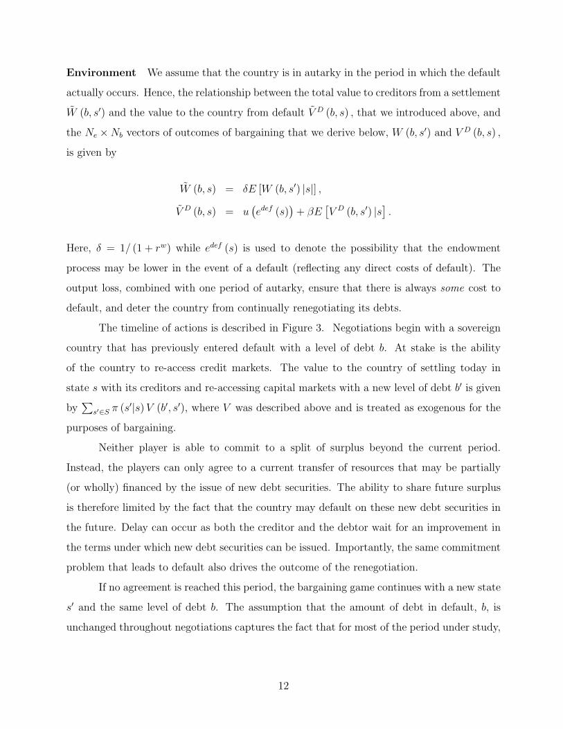
Environment We assume that the country is in autarky in the period in which the default

actually occurs. Hence, the relationship between the total value to creditors from a settlement

W (b, s′) and the value to the country from default V D (b, s) , that we introduced above, and

the Ne ×Nb vectors of outcomes of bargaining that we derive below, W (b, s′) and V D (b, s) ,

is given by

W (b, s) = δE [W (b, s′) |s|] ,

V D (b, s) = u(edef (s)

)+ βE

[V D (b, s′) |s

].

Here, δ = 1/ (1 + rw) while edef (s) is used to denote the possibility that the endowment

process may be lower in the event of a default (reflecting any direct costs of default). The

output loss, combined with one period of autarky, ensure that there is always some cost to

default, and deter the country from continually renegotiating its debts.

The timeline of actions is described in Figure 3. Negotiations begin with a sovereign

country that has previously entered default with a level of debt b. At stake is the ability

of the country to re-access credit markets. The value to the country of settling today in

state s with its creditors and re-accessing capital markets with a new level of debt b′ is given

by∑

s′∈S π (s′|s) V (b′, s′), where V was described above and is treated as exogenous for the

purposes of bargaining.

Neither player is able to commit to a split of surplus beyond the current period.

Instead, the players can only agree to a current transfer of resources that may be partially

(or wholly) financed by the issue of new debt securities. The ability to share future surplus

is therefore limited by the fact that the country may default on these new debt securities in

the future. Delay can occur as both the creditor and the debtor wait for an improvement in

the terms under which new debt securities can be issued. Importantly, the same commitment

problem that leads to default also drives the outcome of the renegotiation.

If no agreement is reached this period, the bargaining game continues with a new state

s′ and the same level of debt b. The assumption that the amount of debt in default, b, is

unchanged throughout negotiations captures the fact that for most of the period under study,

12

interest on missed payments was not a part of default settlements4.

Negotiations between the creditors and the debtor are efficient, in the sense that

agreements are optimal for the two parties subject to the constraints on negotiations implied

by future default risk. To capture this fact, we say that negotiations are privately optimal

ex post. Nonetheless, delay may be said to be socially wasteful ex post, as the country is

unable to access capital markets while in default, and thus forfeits potential gains from trade

in tilting and smoothing its consumption.

Timing and Actions Bargaining occurs according to a randomly alternating offer bar-

gaining game with an outside option available to the debtor. The timing is illustrated in

Figure 2. At any point, the debtor country has the option of paying off the defaulted debt in

full, using any desired mix of current transfers and new debt securities issued at the market

price. We refer to this action as the outside option of the debtor, although we stress that

this is strictly only an outside option for the game conditional on default, and not for the

entire borrowing environment. In addition to being a feature of the actual environment

governing sovereign debt renegotiations, this assumption guarantees that the total value of

the settlement never exceeds b which serves to bound our bond price function.

In every period and in each state of the world s, either the sovereign borrower or

the creditor is selected to be the proposer who is then allowed to make a settlement offer. A

proposal consists of a transfer of resources τ to the creditor in the current period, and an issue

of new debt securities b′. The proposer’s action is therefore given by an offer of two values

(τ , b′) ∈ R× B. We do not place any additional bounds on the issue of new debt, although

debt issues will continue to be limited by the price that new creditors will be prepared to

offer for these new bonds. Importantly, we allow for the possibility that the settlement may

contain an amount of “new money” in which case the country receives a positive flow of the

consumption good in the period in which they settle (this corresponds to a negative τ).

Once a proposal is made, the non-proposing agent chooses to either accept or reject

the current proposal. If the proposal is accepted, or if the debtor country’s outside option is

4In cases that went to court, the courts did not award interest on missed payments until 1997 as part ofthe legal proceedings involving Elliott Associated and Peru.

13

taken, the bargaining concludes and the country emerges from default with the new negotiated

debt level. If the proposal is rejected and the outside option is not taken, the game continues

to the next period, and we say that there has been delay in bargaining. In the next period,

the realization of the state determines the identity of the proposer, and the timing repeats

with the next proposer suggesting an offer.

A history of the bargaining game is a list of all previous actions and states that have

occurred after a country’s most recent default. That is, we are assuming that each debt

restructuring is not affected by previous borrowing, default or debt restructurings, except

insofar as these decisions have determined the debt level b. If no offer has been accepted,

and if t indexes stages, a history up to the beginning of stage t is defined by the sequence of

realizations for the state variable and the sequence of rejected offers:

ht ={

st = (s0, s1, ..., st−1) , (τ , b′)t=((τ 0, b

′0) , (τ 1, b

′1) , ...,

(τ t−1, b

′t−1

))}.

We let H t denotes the set of all histories to stage t.

Strategies Strategies map the level of the defaulted debt b and the history into a choice

of actions. The current state determines the identity of the current proposer, and the set

of feasible actions depends on which player is the proposer. A strategy for the creditor

when they are the proposer is a function σC,P : B×H t × S → R×B. The situation is more

complicated when the debtor is the proposer due to the fact that the debtor may elect to take

the outside option. In particular, a strategy for the debtor when they are the proposer is a

function σD,P : B×H t×S → R×B×{0, 1} , where the third element takes on the value one if

the debtor takes the outside option; whether or not the debtor takes the outside option, there

is an associated transfer and new debt level (τ , b′) . A strategy for the creditor when they are

not the proposer depends on whether or not the debtor has taken the outside option. If the

debtor has not taken the outside option, a strategy for a non-proposing creditor is a function

σC,NP : B × H t+1 → {0, 1} where 0 denotes rejection of the proposal, and 1 acceptance of

the proposal. If the debtor has taken the outside option, the creditor has no choice but to

accept the proposed settlement and so a strategy for a non-proposing creditor is a function

14

σC,NP : B × H t+1 → {1}. A strategy for the debtor when they are not the proposer is

a function σD,NP : B × H t+1 → {0} ∪ {1} ∪ {2} × {(τ , b′) ∈ R×B : τ + q (b′, st+1) b′ ≥ b}

where the first element 0 indicates a rejection, 1 indicates acceptance, and the third element

indicates that the outside option was chosen with associated transfer and new debt levels

(τ , b′). A strategy profile is a pair of strategies, one for each player.

Payoffs and Equilibrium Next we discuss outcomes and payoffs and define an equilib-

rium. An outcome is a termination of negotiations plus the final accepted offer. That is, an

outcome of the bargaining game is a stopping time t∗ and the associated proposal (τ , b′) . At

any history, a strategy profile induces an outcome and hence a payoff for each player. The

payoff to the debtor given outcome ϕ = {t∗, (τ , b′)} after history st∗ is

V D(t∗, st∗ , (τ , b′)

)=

t∗−1∑r=0

βru(edef (sr)

)+ βt∗

{u(edef (st∗)− τ

)+ βE [V (b′, st∗+1) |st∗ ]

},

while to the creditor it is given by

W(t∗, st∗ , (τ , b′)

)= δt∗ {τ + q (b′, st∗) b′} .

Let G(b, ht) denote the game from date t onwards starting from history ht. Let |ht

denote the restriction to the histories consistent with ht. Then σ|ht is a strategy profile

on G(b, ht). We let ϕ (σ|ht) be the outcome generated by the strategy profile σ|ht in game

G (b, ht) . A strategy profile is subgame perfect (SP) if, for every history ht, σ|ht is a Nash

equilibrium of G(b, ht). That is

W(ϕ(σ|ht

))≥ W

(ϕ(σD|ht, σC′|ht

)),

V D(ϕ(σ|ht

))≥ V D

(ϕ(σD′|ht, σC |ht

)),

for all σ, t, and ht.

As is customary in the literature, we impose the restriction of stationarity. A strategy

profile is stationary if the actions prescribed at any history depend only on the current state

15

and proposal. That is a stationary strategy profile satisfies:

σD(b, ht, st

)= σD (b, st)

σC(b,(ht, (st, (τ t, b

′t))))

= σC (b, st, (τ t, b′t)) ,

for all ht and all t when st is such that the debtor proposes, and

σC(b, ht, st

)= σC (b, st)

σD(b,(ht, (st, (τ t, b

′t))))

= σD (b, st, (τ t, b′t)) ,

for all ht and all t when st is such that the creditor proposes. A stationary subgame perfect

equilibrium (SSP) outcome and payoff are the outcome and payoff generated by an SSP

strategy profile. We define a stationary outcome as ((B × S)µ , µ),where µ = (τ , b′) and

where (B × S)µ is the set of debt levels b and states s on which an agreement occurs or the

outside option is taken, and where (B × S) \ (B × S)µ is the disagreement set.

3.B Solution to the Bargaining Model

The solution to the overall model involves solving a fixed point problem. First, taking

as given the solution to the bargaining problem, we solve for the solution to the debtor

countries default problem and update the market price of debt. Second, we take the market

price of debt and the debtor’s value function from repayment and then use these to solve the

bargaining problem. An equilibrium is a fixed point of the composition of the two operators.

In this section, we focus on the bargaining model, taking as given the form of the solution to

the borrowing problem.

Recursive Problem Statement

For this section, we take the solution to the borrowing problem as given. That is, the

debtor country’s value of accessing capital markets V (b, s) is assumed to be a fixed element

of the set all real valued Ne by Nb vectors, and the equilibrium bond price function q (b, s) is

assumed to be a fixed element of Q (B × S). Given these assumptions, we then show that

the SSP values of the bargaining game are fixed points of a particular functional equation.

16

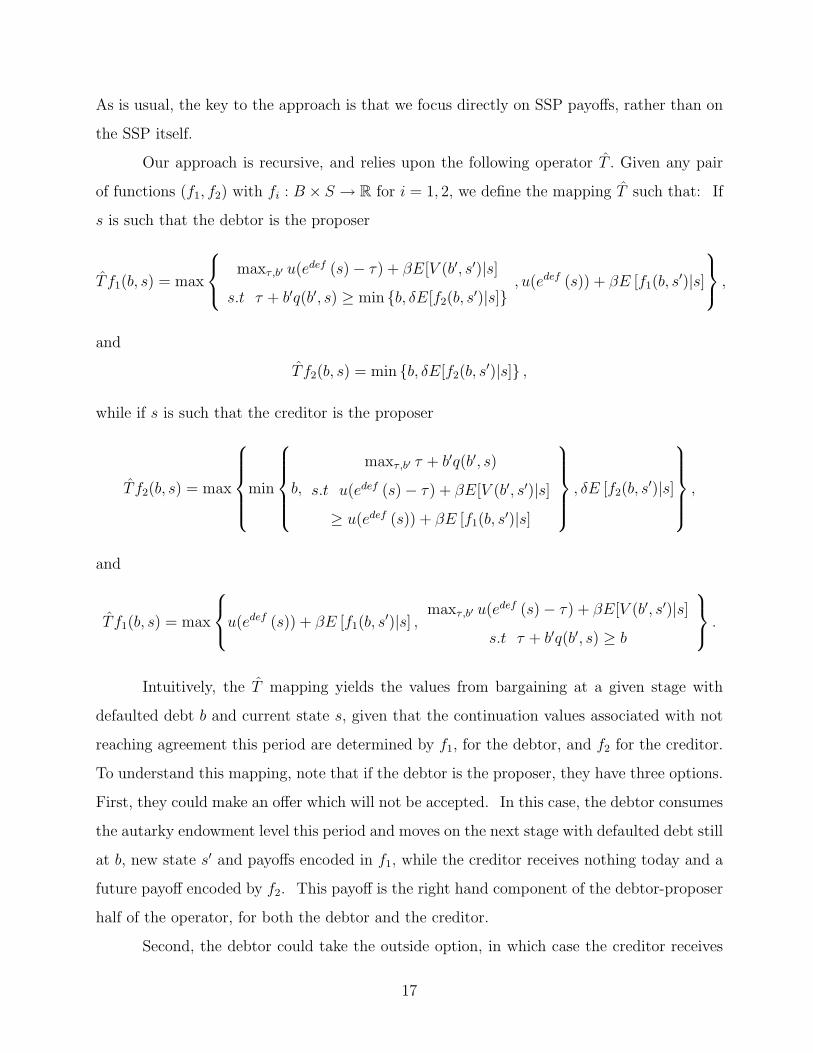
As is usual, the key to the approach is that we focus directly on SSP payoffs, rather than on

the SSP itself.

Our approach is recursive, and relies upon the following operator T . Given any pair

of functions (f1, f2) with fi : B × S → R for i = 1, 2, we define the mapping T such that: If

s is such that the debtor is the proposer

T f1(b, s) = max

maxτ,b′ u(edef (s)− τ) + βE[V (b′, s′)|s]

s.t τ + b′q(b′, s) ≥ min {b, δE[f2(b, s′)|s]}

, u(edef (s)) + βE [f1(b, s′)|s]

,

and

T f2(b, s) = min {b, δE[f2(b, s′)|s]} ,

while if s is such that the creditor is the proposer

T f2(b, s) = max

min

b,

maxτ,b′ τ + b′q(b′, s)

s.t u(edef (s)− τ) + βE[V (b′, s′)|s]

≥ u(edef (s)) + βE [f1(b, s′)|s]

, δE [f2(b, s′)|s]

,

and

T f1(b, s) = max

u(edef (s)) + βE [f1(b, s′)|s] ,

maxτ,b′ u(edef (s)− τ) + βE[V (b′, s′)|s]

s.t τ + b′q(b′, s) ≥ b

.

Intuitively, the T mapping yields the values from bargaining at a given stage with

defaulted debt b and current state s, given that the continuation values associated with not

reaching agreement this period are determined by f1, for the debtor, and f2 for the creditor.

To understand this mapping, note that if the debtor is the proposer, they have three options.

First, they could make an offer which will not be accepted. In this case, the debtor consumes

the autarky endowment level this period and moves on the next stage with defaulted debt still

at b, new state s′ and payoffs encoded in f1, while the creditor receives nothing today and a

future payoff encoded by f2. This payoff is the right hand component of the debtor-proposer

half of the operator, for both the debtor and the creditor.

Second, the debtor could take the outside option, in which case the creditor receives

17

the value of the defaulted debt b, and the debtor receives the maximum value achievable

while still delivering a payoff of b to the creditor. This corresponds to the left hand side of

the creditors part of the debtor-proposer half of the operator, and to the left hand side of the

debtor’s part of the operator given the constraint on creditor utility defined by b.

Third, the debtor could make an offer that is accepted. In this case, since the debtor

makes the offer, the creditor receives none of the surplus from the agreement, and hence

receives the same payoff as if the offer was not accepted (the right hand side of the creditor

part of the debtor-proposer half of the operator). The debtor, on the other hand, receives

the maximum value that can be achieved while delivering this value to the creditor (the left

hand side of the debtor’s part of the operator with the constraint defined by the reservation

payoff of the creditor). Since the debtor would never take the outside option when it can do

better by making an offer that is accepted, the minimum over the value of the debt and the

creditors reservation value is the relevant determinant of the constraint.

Similar logic underlies the half of the operator that applies to states in which the

creditor is the proposer, noting that the creditor will extract all of the surplus from an

accepted proposal up to a maximum value of b at which level the debtor will take the outside

option.

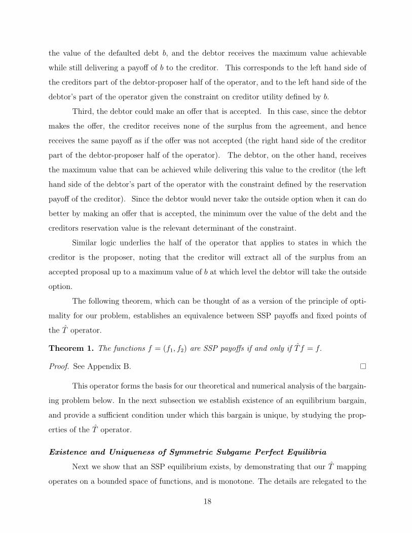
The following theorem, which can be thought of as a version of the principle of opti-

mality for our problem, establishes an equivalence between SSP payoffs and fixed points of

the T operator.

Theorem 1. The functions f = (f1, f2) are SSP payoffs if and only if T f = f.

Proof. See Appendix B.

This operator forms the basis for our theoretical and numerical analysis of the bargain-

ing problem below. In the next subsection we establish existence of an equilibrium bargain,

and provide a sufficient condition under which this bargain is unique, by studying the prop-

erties of the T operator.

Existence and Uniqueness of Symmetric Subgame Perfect Equilibria

Next we show that an SSP equilibrium exists, by demonstrating that our T mapping

operates on a bounded space of functions, and is monotone. The details are relegated to the

18

appendix.

Theorem 2. An SSP equilibrium exists.

Proof. See Appendix B.

The uniqueness of the values of the equilibrium bargain could be easily established if T

is a contraction mapping. However, as in many multi-agent problems, this is not straightfor-

ward. The difficulty results from two issues. First, changes in one agent’s continuation value

function will affect the result of the operator on the other agents continuation value function,

because continuation values act as constraints on the proposals that will be accepted. Second,

and more importantly, the rates at which changes in one agent’s continuation value affect

the operator on the other agents continuation value can vary when payoffs are non-linear

functions of outcomes.

To understand this difficulty, it is instructive to consider how these issues appear in

an attempt to establish Blackwell’s sufficient conditions for a contraction mapping, and in

particular by affecting the proof of the discounting condition. Suppose we change the value of

the creditor’s and debtor’s continuation values by a small constant amount. The discounting

property requires that the operator produce functions that are bounded by the modulus of

the contraction mapping, which is strictly less than one. Since the country’s felicity function

is non-linear, it is possible that a small increase in the creditor’s continuation value, which

would lead to a small change in the settlement value, could lead to a large change in the

country’s payoff if the marginal utility of consumption was high near the solution of the

debtor’s problem in the debtor’s half of the T operator. Moreover, it is also possible that a

small change in the debtor’s continuation value could result in a large change in the value of

the settlement (and hence also a large change in creditor payoffs) if the marginal utility of

consumption is low near the solution of the creditor’s problem in the creditor’s half of the T

operator.

The following theorem states a condition that is sufficient to prove uniqueness, by

imposing bounds on the rate at which resources can be transformed into utility, and the rate

at which utility can be transformed into resources. As a consequence of the fact that we have

imposed few restrictions on the shape of the V and q functions, the condition is stated in terms

19

of bounds on the slope of the utility function of the debtor. In our numerical work below, as in

much of the quantitative literature on sovereign debt and default, we focus on discount factors

for the country that are substantially less than one, reflecting political economy problems in

developing countries that lead to impatient policy making. For sufficiently low β, we can

typically show that the sufficient condition is satisfied.

Theorem 3. Let u : R → R be differentiable. If there exists KL > β and KU < 1/δ such

that KL ≤ u′ (c) ≤ KU , for all c, then the SSP equilibrium values are unique.

Proof. See Appendix B.

3.C Solution to Borrowing Model

In the previous section, we establish the existence and uniqueness of a solution to

the debt restructuring bargaining problem, taking as given the value to the country from

re-accessing capital markets with new debt b′, E [V (b′, s′) |s] , and the value of new debt to

creditors q (b′, s) . In this section, we take as given the solution to the bargaining model, and

hence the value to the country and the creditor from being in default, and then establish

existence of a solution to the borrowing problem. That is, we take as given the Ne × Nb

vectors of payoffs to the country, V D (b, s) , and the creditor, W (b, s) , in default, that are

elements of B (B × S) .

The solution of the borrowing problem is established as the composition of two op-

erators. The first takes a value to the country from default and an equilibrium bond price

function, and then solves the country’s problem to obtain a value to the country for access

to capital markets, and a default policy function, which is a selection from a default policy

correspondence. The second takes the default policy function and combines it with the value

to the creditors from default to obtain a new bond price function. Existence of a solution

follows from the monotonicity of the composition of these operators.

Theorem 4. Given(V D (b, s) , W (b, s)

)∈ B (B × S) and q (b, s) ∈ Q (B × S) , there exists

a value function for the country, V (b, s) , and an equilibrium bond price function q (b, s) ∈

Q (B × S) , that solve the borrowing problem.

Proof. See Appendix B.

20

Given the result of this Theorem, it is tempting to try to prove existence of an equilib-

rium for our entire model by iterating successively on the T V , T q and T operators. However,

this approach need not converge. Specifically, although iterating on the T V and T q op-

erators produces a monotone operator, when combined with the bargaining operator, the

compounded operator need not be monotone. Intuitively, it can be the case that a high

value to the creditor in default, and a low value to debtor, leads to a high bond price, which

in turn leads to a high value to the country from repayment. This high value to repayment

can lead to a high value from default, which then leads to a low bond price in the next

iteration. That is, we cannot rule out cycles in the successive application of these operators.

In the next section, we describe an alternative method for proving existence.

3.D Existence of Equilibrium

In this section, we establish the existence of a recursive equilibrium for our economy.

First, we define an equilibrium for our economy.

Definition 1. An equilibrium for our economy is a value function for the country from

borrowing V (b, s), a value function for the country in default V D (b, s) , a value function for

the creditor in default W (b, s) and a bond price function q (b, s) such that:

1. Given the bond price function q (b, s) and the value to the country from re-accessing

capital markets V (b, s), the country and the creditor optimally bargain over re-access to

financial markets. That is, V D and W are fixed points of the inside default operator

T ;

2. Given the value to the country and from default V D (b, s), and the bond price q (b, s) , the

country makes optimal borrowing and default decisions. That is, V (b, s) is a fixed point

of T V with associated default policy correspondence Φ (b, s)

3. Given the payoff to the creditor in default W and the optimal default policy correspon-

dence, the bond price function q (b, s) satisfies the no arbitrage condition for creditors.

That is, q (b, s) is a fixed point of the operator T q.

The latter two conditions may equivalently be written as: Given V D (b, s) and W (b, s) ,

V (b, s) and q (b, s) are a fixed point of the outside default operator, which is the composition

21

of the T V and T q operators.

We prove existence by using the operators defined above to construct a new mapping

from the space of value functions for the country and creditor in default, and the space of

bond price functions, into itself, and establishing that it possesses a fixed point. Specifically,

define the mapping H from B (B × S)×Q (B × S) into itself as follows. First, given V D, W

and q, iterate on the outside default operator to convergence to obtain a new bond price

function q′ (b, s) . Second, given V D and q, iterate on the T V operator to convergence to

produce a value function V. Then, given the old q and this V, iterate on the T operator to

convergence to find new V D′ and W ′. We establish that the combination of these operators

defines an upper hemi-continuous correspondence with non-empty and convex values. Then,

noting that B (B × S) × Q (B × S) is a compact and convex space of functions, the result

then follows by application of the Kakutani-Fan-Glicksberg fixed point theorem.

Theorem 5. There exists an equilibrium of our borrowing economy.

Proof. See Appendix B.

4 Calibration and Numerical Results

In this section, we present results from several numerical solutions of the model that

vary only in the calibration of the bargaining power process for the debtor and creditor. These

examples are used to illustrate some comparative static properties of the model, and to build

intuition for the elements of the model that produce delay. We then present our benchmark

case in which the parameters of the model governing bargaining power are calibrated to some

aspects of the relationship between default and output observed in the data. The model is

then assessed according to it’s ability to match the other facts discussed in the introduction.

4.A Calibration

The first step in calibrating the model is the choice of a period length. On the one

hand, as debt contracts in our theory are one period in duration, calibration to a long period

length is necessary in order to match the maturity of observed debt issues. A long period

length is also desirable given that the information on which bargaining positions are formed is

revealed at best quarterly, and in some cases only annually. On the other hand, the bargaining

22

process plausibly operates at a high frequency, suggesting that we should calibrate to a shorter

period length. To balance these concerns, and given that most other studies in the literature

calibrate to quarterly data, we adopt a quarterly calibration.

In some cases, our data is only available at an annual frequency. To construct annual

outcomes, we simulate on a quarterly calendar for 11000 periods beginning with the March

quarter, and drop the first thousand periods to eliminate the effect of initial conditions.

All model variables are treated identically to the data, with flow variables such as output

being summed, and stock variables such as debt calculated as of the end of the year. Trend

output is computed from the annualized data using a Hodrick-Prescott filter with smoothing

parameter equal to 6.25 as in Ravn and Uhlig (2002). If a country exits and re-enters default

in successive quarters, we count this as one default5. Since our data measures the start and

end of a default at a high frequency, we calculate the duration of default in the model from the

quarterly data. In comparing our annual data on output and debt to the timing of defaults

and settlements, we follow the practice of S&P and label a country as being in default in a

given year if it was in default at any point in that year.

Most parameters in the model are held constant in every experiment and, as shown

in Table 3, are set to values that are standard in the literature. Following Arellano (2007),

Aguiar and Gopinath (2006), Yue (2007), and Tomz and Wright (2007), the world interest

rate is set to 1% per quarter, and the coefficient of relative risk aversion is set to two. The

income process is assumed to follow a log normal AR(1) process, which is chosen to match

Argentinean output data. One non-standard parameter value is the discount factor, which in

the rest of the literature often takes on values as low as 0.8 for quarterly data implying annual

discount factors around 0.4. Although a low value can be plausibly motivated by political

economy considerations that lead developing country governments to act myopically, we view

a choice of 0.8 as too extreme and use a more modest 0.945 at our quarterly frequency.

5This is conventional. Standard and Poors classify periods in which a country has engaged in a series ofsuccessive renegotiations as one default episode. For example, S&P defines Mexico to have defaulted oncein the past three decades, starting in 1982 and ending in 1990, despite the fact that Arteta and Hale (2008)record 3 separate negotiations and 23 separate rescheduling agreements for commercial bank debt during thisperiod. Likewise, Beim and Calomiris (2001, p.35) treat defaults occurring within five years of each other asone default episode. By only merging defaults that occur within one quarter of each other, our estimates ofdelay are conservative.

23

The remaining parameters describe the evolution of the proposer identity during bar-

gaining, and the loss of output experienced by the country during default. For our benchmark

case, these parameters are calibrated to the features of the data summarized in Table 4. First,

we calibrate the output loss during default to match the observed average ratio of debt to

GDP; higher output costs support higher borrowing levels. In matching model data on debt

to the World Bank data on debt, we must confront a measurement issue, raised earlier and

described in more detail in Appendix C. The issue is that the World Bank reports debt at

face values, which is defined as the undiscounted sum of all future amortization payments.

However, two equivalent debts (that is, two debts with exactly the same streams of debt

service) will have different face values if debt service is divided into principal and interest in

different ways. In our presentation of the theory, all debt is issued at a discount without a

coupon, so the face value of the debt is given by the state variable b. However, these zero-

coupon bonds with face value b are equivalent to par bonds with face value equal to their

market value, q (b, s) b, and with total coupons worth b − q (b, s) b. We calibrate the output

cost of default so that a 2 : 1 weighted average of face value and market value debt matches

the average debt-to-GDP level of 65%, reported by the World Bank. This produces an output

cost of 1% of GDP, which is about half the level assumed by other studies.

Finally, we need to choose values for the parameters governing the evolution of the

identity of the proposer in bargaining. Obviously, the ability to make today’s offer can

be thought of as giving the proposer more bargaining power. Less obviously, the agent’s

expectations about who will propose offers in the future has the strongest effect on bargaining

power because it determines the reservation value of the non-proposing agent. Hence, we

refer to these probabilities as “bargaining power” parameters. Since the economics literature

provides little guidance as to how to set these parameters, we experiment with a number of

alternatives.

In our benchmark case, we calibrate bargaining power to some aspects of the rela-

tionship between default and income in the data. Specifically, we divide output realizations

equally into ‘high’, ‘medium’ and ‘low’ levels, and describe the evolution of proposer iden-

tity in terms of the probability that the debtor proposes conditional on the output level and

identity of the proposer in the previous period. This leaves us six probabilities to calibrate.

24

We assume a limited form of symmetry to set two of these parameters; we assume that the

probability that the creditor proposes tomorrow given that they proposed today and output

was high (low) is equal to the probability that the debtor will propose tomorrow given that

they proposed today and output was low (high). The remaining probabilities are set to match

the first four moments in Table 4, with the resulting probabilities tabulated in Table 5.

In order to build intuition for the effect of bargaining power on the outcomes of the

model, we also present numerical results for five stylized example processes for bargaining

power. The economics literature that considers bargaining typically assumes that bargaining

power is constant (for example, when the cooperative Nash bargaining solution is imposed, as

in Yue (2007) in her study of sovereign debt restructuring). To capture this case, we present

results for two examples in which the identity of the proposer is i.i.d., and which differ only

as to whether it is the creditor (probability 0.99) or debtor (probability 0.55) who is always

likely to propose, and hence who has most of the bargaining power. We follow these i.i.d.

cases with a “persistent” regime where the proposer today is very likely (probability 0.99) to

remain proposer tomorrow, so that there will be random cycles in bargaining power.

Last, we present two examples in which the bargaining power of the agents depends

on economic conditions in the country. In the first case, which we follow the international

relations literature in referring to as “strength through weakness”, the likelihood that the

country is able to make offers in the future is higher when output is low, so that the debtors

bargaining power is greatest when the economy is weak. This case attempts to capture the

idea that in countries with weak economies, the politicians negotiating the debt restructuring

are too weak politically at home to propose significant concessions to its lenders, which acts

as a form of bargaining power. In the second – “strength through strength” – the debtor

country has more bargaining power when output is high, capturing the idea that strong

economic performance insulates a political leader from domestic political pressures. In both

of these cases, the agent that has higher bargaining power when output in the debtor country

is high proposes with a probability greater than one half (probability 0.96). Inspection of the

calibrated probabilities in Table 5 reveals that the benchmark case possesses elements of the

“persistent” and “strength through weakness” examples.

25

4.B Intuition For Delays in Bargaining

Before turning to our results for the benchmark model, it is instructive to examine

bargaining outcomes for two of the example bargaining power processes introduced above.

We begin with an i.i.d. case in which the creditor is very likely to propose each period

and hence has the greater bargaining power. As the likelihood of making future offers is

constant,bargaining power is constant, and defaults are driven primarily by fluctuations in

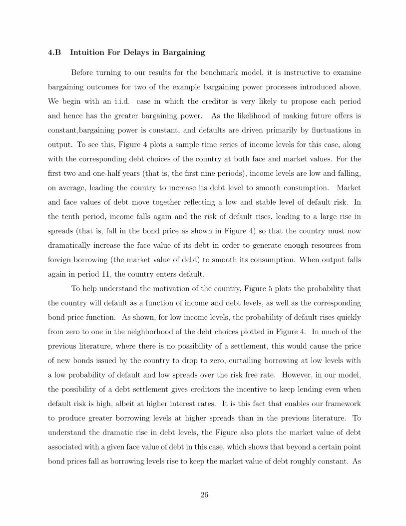
output. To see this, Figure 4 plots a sample time series of income levels for this case, along

with the corresponding debt choices of the country at both face and market values. For the

first two and one-half years (that is, the first nine periods), income levels are low and falling,

on average, leading the country to increase its debt level to smooth consumption. Market

and face values of debt move together reflecting a low and stable level of default risk. In

the tenth period, income falls again and the risk of default rises, leading to a large rise in

spreads (that is, fall in the bond price as shown in Figure 4) so that the country must now

dramatically increase the face value of its debt in order to generate enough resources from

foreign borrowing (the market value of debt) to smooth its consumption. When output falls

again in period 11, the country enters default.

To help understand the motivation of the country, Figure 5 plots the probability that

the country will default as a function of income and debt levels, as well as the corresponding

bond price function. As shown, for low income levels, the probability of default rises quickly

from zero to one in the neighborhood of the debt choices plotted in Figure 4. In much of the

previous literature, where there is no possibility of a settlement, this would cause the price

of new bonds issued by the country to drop to zero, curtailing borrowing at low levels with

a low probability of default and low spreads over the risk free rate. However, in our model,

the possibility of a debt settlement gives creditors the incentive to keep lending even when

default risk is high, albeit at higher interest rates. It is this fact that enables our framework

to produce greater borrowing levels at higher spreads than in the previous literature. To

understand the dramatic rise in debt levels, the Figure also plots the market value of debt

associated with a given face value of debt in this case, which shows that beyond a certain point

bond prices fall as borrowing levels rise to keep the market value of debt roughly constant. As

26

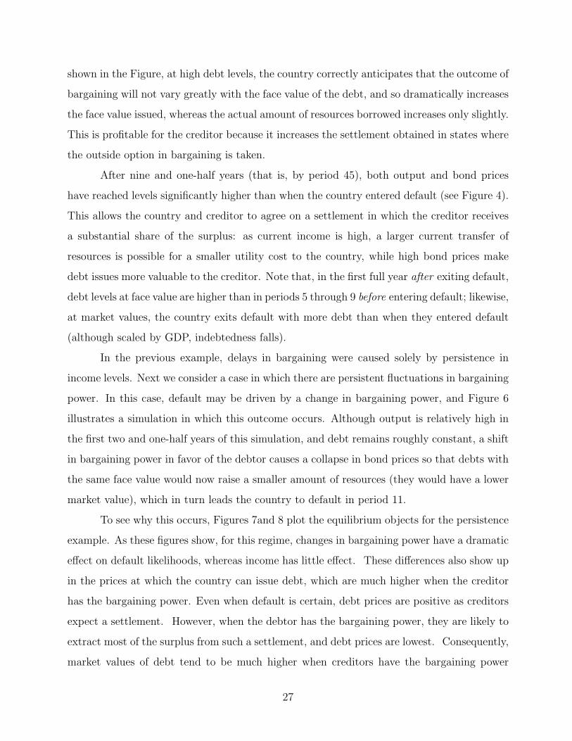
shown in the Figure, at high debt levels, the country correctly anticipates that the outcome of

bargaining will not vary greatly with the face value of the debt, and so dramatically increases

the face value issued, whereas the actual amount of resources borrowed increases only slightly.

This is profitable for the creditor because it increases the settlement obtained in states where

the outside option in bargaining is taken.

After nine and one-half years (that is, by period 45), both output and bond prices

have reached levels significantly higher than when the country entered default (see Figure 4).

This allows the country and creditor to agree on a settlement in which the creditor receives

a substantial share of the surplus: as current income is high, a larger current transfer of

resources is possible for a smaller utility cost to the country, while high bond prices make

debt issues more valuable to the creditor. Note that, in the first full year after exiting default,

debt levels at face value are higher than in periods 5 through 9 before entering default; likewise,

at market values, the country exits default with more debt than when they entered default

(although scaled by GDP, indebtedness falls).

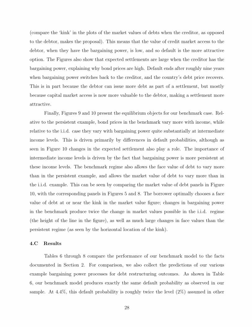
In the previous example, delays in bargaining were caused solely by persistence in

income levels. Next we consider a case in which there are persistent fluctuations in bargaining

power. In this case, default may be driven by a change in bargaining power, and Figure 6

illustrates a simulation in which this outcome occurs. Although output is relatively high in

the first two and one-half years of this simulation, and debt remains roughly constant, a shift

in bargaining power in favor of the debtor causes a collapse in bond prices so that debts with

the same face value would now raise a smaller amount of resources (they would have a lower

market value), which in turn leads the country to default in period 11.

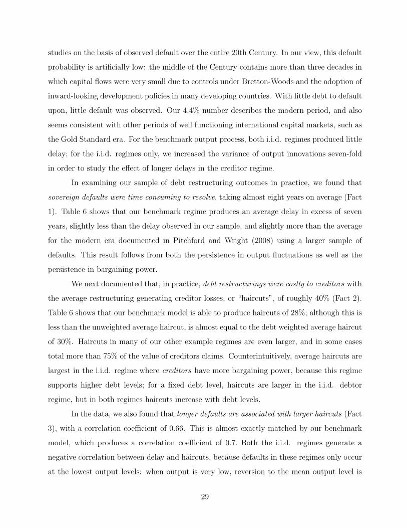
To see why this occurs, Figures 7and 8 plot the equilibrium objects for the persistence

example. As these figures show, for this regime, changes in bargaining power have a dramatic

effect on default likelihoods, whereas income has little effect. These differences also show up

in the prices at which the country can issue debt, which are much higher when the creditor

has the bargaining power. Even when default is certain, debt prices are positive as creditors

expect a settlement. However, when the debtor has the bargaining power, they are likely to

extract most of the surplus from such a settlement, and debt prices are lowest. Consequently,

market values of debt tend to be much higher when creditors have the bargaining power

27

(compare the ‘kink’ in the plots of the market values of debts when the creditor, as opposed

to the debtor, makes the proposal). This means that the value of credit market access to the

debtor, when they have the bargaining power, is low, and so default is the more attractive

option. The Figures also show that expected settlements are large when the creditor has the

bargaining power, explaining why bond prices are high. Default ends after roughly nine years

when bargaining power switches back to the creditor, and the country’s debt price recovers.

This is in part because the debtor can issue more debt as part of a settlement, but mostly

because capital market access is now more valuable to the debtor, making a settlement more

attractive.

Finally, Figures 9 and 10 present the equilibrium objects for our benchmark case. Rel-

ative to the persistent example, bond prices in the benchmark vary more with income, while

relative to the i.i.d. case they vary with bargaining power quite substantially at intermediate

income levels. This is driven primarily by differences in default probabilities, although as

seen in Figure 10 changes in the expected settlement also play a role. The importance of

intermediate income levels is driven by the fact that bargaining power is more persistent at

these income levels. The benchmark regime also allows the face value of debt to vary more

than in the persistent example, and allows the market value of debt to vary more than in

the i.i.d. example. This can be seen by comparing the market value of debt panels in Figure

10, with the corresponding panels in Figures 5 and 8. The borrower optimally chooses a face

value of debt at or near the kink in the market value figure; changes in bargaining power

in the benchmark produce twice the change in market values possible in the i.i.d. regime

(the height of the line in the figure), as well as much large changes in face values than the

persistent regime (as seen by the horizontal location of the kink).

4.C Results

Tables 6 through 8 compare the performance of our benchmark model to the facts

documented in Section 2. For comparison, we also collect the predictions of our various

example bargaining power processes for debt restructuring outcomes. As shown in Table

6, our benchmark model produces exactly the same default probability as observed in our

sample. At 4.4%, this default probability is roughly twice the level (2%) assumed in other

28

studies on the basis of observed default over the entire 20th Century. In our view, this default

probability is artificially low: the middle of the Century contains more than three decades in

which capital flows were very small due to controls under Bretton-Woods and the adoption of

inward-looking development policies in many developing countries. With little debt to default

upon, little default was observed. Our 4.4% number describes the modern period, and also

seems consistent with other periods of well functioning international capital markets, such as

the Gold Standard era. For the benchmark output process, both i.i.d. regimes produced little

delay; for the i.i.d. regimes only, we increased the variance of output innovations seven-fold

in order to study the effect of longer delays in the creditor regime.

In examining our sample of debt restructuring outcomes in practice, we found that

sovereign defaults were time consuming to resolve, taking almost eight years on average (Fact

1). Table 6 shows that our benchmark regime produces an average delay in excess of seven

years, slightly less than the delay observed in our sample, and slightly more than the average

for the modern era documented in Pitchford and Wright (2008) using a larger sample of

defaults. This result follows from both the persistence in output fluctuations as well as the

persistence in bargaining power.

We next documented that, in practice, debt restructurings were costly to creditors with

the average restructuring generating creditor losses, or “haircuts”, of roughly 40% (Fact 2).

Table 6 shows that our benchmark model is able to produce haircuts of 28%; although this is

less than the unweighted average haircut, is almost equal to the debt weighted average haircut

of 30%. Haircuts in many of our other example regimes are even larger, and in some cases

total more than 75% of the value of creditors claims. Counterintuitively, average haircuts are

largest in the i.i.d. regime where creditors have more bargaining power, because this regime

supports higher debt levels; for a fixed debt level, haircuts are larger in the i.i.d. debtor

regime, but in both regimes haircuts increase with debt levels.

In the data, we also found that longer defaults are associated with larger haircuts (Fact

3), with a correlation coefficient of 0.66. This is almost exactly matched by our benchmark

model, which produces a correlation coefficient of 0.7. Both the i.i.d. regimes generate a

negative correlation between delay and haircuts, because defaults in these regimes only occur

at the lowest output levels: when output is very low, reversion to the mean output level is

29

fast and settlements occur quickly; however, when output is low, haircuts are large. This

also explains why there is a negative correlation between output declines and delay for the

i.i.d. models, with the largest output declines being associated with the fastest reversion

to the mean, and hence the shortest delays. The other example bargaining power regimes

produce little or no relationship between output declines in the year of default and debt

restructuring outcomes, in contrast to the data where larger output declines in the year of

default are associated with longer defaults and larger haircuts (Fact 4). Our benchmark model

produces negative correlations between the change in output and both haircuts and delays.

The reason is that, in the benchmark model, defaults occur for two reasons: when bargaining

power changes at intermediate income levels, defaults are resolved with little delay and small

haircuts because creditors regain bargaining power relatively quickly; when income falls to

low levels, defaults are resolved more slowly and with larger haircuts, because there is more

persistence in the output process. In our other example regimes, only one effect is present

so that time aggregation tends to reduce or eliminate the correlation between outcomes and

output.

In calibrating the bargaining power process, we chose parameter values to match some

aspects of the relationship between output and default in the data, although not the aspects

that we had emphasized in Section 2, where we had confirmed the finding of Tomz and

Wright (2007) that defaults are somewhat more likely to occur when output is below trend,

and settlements tend to occur when output has returned to trend (Fact 5). Table 7 shows

that our benchmark model also produces a weak relationship between output and default,

as observed in the data, although settlements tend to occur before output returns to trend.

The weak relationship between default and output is also a feature of each of our example

bargaining regimes. However, whereas for many of our example regimes this is solely a

product of time aggregation, for our benchmark regime it is also due to the role of switches

in bargaining power in generating defaults. As shown in Table 8, at a quarterly frequency,

all of our examples except for the strength-through-strength regime produce a near perfect

negative relationship between default and output. Moving from quarterly to annual data

not only weakens this pattern, but occasionally reverses it. By contrast, our benchmark

regime displays a strong negative relationship in only the quarter of default, and almost no

30

relationship with output in the preceding quarter.

Finally, we documented that in practice debt restructuring negotiations are ineffective

at reducing country indebtedness (Fact 6) with the median country exiting default with 5%

more debt (scaled by GDP) than when it entered default, and the mean country exiting

with 25% more debt. Table 7 presents results on the evolution of indebtedness throughout

default for each of the bargaining regimes. Data on debt is presented at both at face values

and market values in order to bracket the World Bank data which, as discussed above and

in Appendix C, is an average of the two. Our benchmark regime predicts that a country

should exit default with roughly the same level of indebtedness as when they entered default,

regardless of which measure of the value of debt is used. This is because settlements tend

to be associated with both improved economic conditions and more bargaining power for the

creditor, which increase the country’s ability to borrow.

To summarize, we conclude that our benchmark model is able to explain almost all

of the delay observed in the data and more than two-thirds of observed haircuts, while also

producing the relationships between bargaining outcomes and economic activity documented

above in Section 2. In addition to matching these new facts, our model is also able to match

the features of the data emphasized by the previous quantitative theoretical literature on

sovereign default. Specifically, this literature has emphasized four facts, all established using

quarterly (and chiefly Argentine) data; we collect these facts in Table 9. First, capital

flows tend to be “procyclical”, with net exports relatively high (and hence capital inflows

small) when output is relatively low; the correlation coefficient in the quarterly Argentine

data has been reported between −0.2 and −0.9. Second, the difference between interest

rates charged on developing country and developed country debts, typically referred to the

‘spread’ on developing country debt, is counter-cyclical, rising in recessions and falling in

booms, with estimates of the correlation between spreads and output for Argentina ranging

from −0.1 to −0.9. Third, high spreads are associated with capital outflows, with correlation

coefficients between spreads and net exports reported between 0.05 and 0.85. Fourth and

finally, consumption in many developing countries is more volatile than output, with the

standard deviation of consumption roughly 10 percentage points higher than the standard

deviation of output.

31

Table 9 documents the performance of both our benchmark model and our expository

examples along these dimensions and compares them to results reported in a sample of other

studies. All moments were calculated from the quarterly model data. Our benchmark model,

like some of the leading previous studies, produces consumption that is almost exactly 10%

more volatile than output. This arises due to the large movements in consumption that

are predicted in both the year of default and the year of settlement. All regimes, except

for strength-through-strength, produce countercyclical spreads, with the benchmark model

producing a correlation between spreads and income that is almost exactly in the center

of the range of published targets. Likewise, the benchmark model also produces procyclical

capital flows with the correlation between income and capital flows the same as that produced

by Arellano (2007). All of the regimes produce a positive relationship between spreads and

capital flows, with the benchmark model producing a stronger relationship, closer to that

observed in the data, than any of the alternative studies.

Finally, a number of studies have emphasized the inability of quantitative models of

sovereign debt to produce spreads with the same level, and volatility, as observed in the

data (see, for example, Arellano and Ramnarayan 2008, Chatterjee and Eyigungor 2008, and

Hatchondo and Martinez 2008). In assessing the ability of this class of models to match data

on spreads, it is important to note that the available data on spreads are limited. Prior to the

early 1990s, most developing country borrowing took the form of bank loans that were not

traded on liquid markets. Moreover, many developing countries spent the decade of the 1980s

in default, so that the data on spreads in the 1990s should be viewed as being conditional on

a recent settlement of a default. In the case of Argentina, spreads in the 1990s should also

be viewed as conditional on being in the lead-up to another default6. Bearing these caveats

in mind, a coarse summary of the Argentine data over this period shows that Argentine

spreads averaged 5 percentage points during the 1990s, peaking near 15 percentage points in

the middle of 1995 and again just prior to the default at the end of 2001. The benchmark

calibration of our theory produces spreads on the order of those observed in the Argentine

6In recognition of this problem, most authors follow Arellano (2007, p.22) and restrict attention to simu-lations that are less than eighty quarters in length and terminate just prior to a default, so as to match theavailable quarterly data for Argentina. As shown in her Figure 5, the spreads generated by her model forthis period are typically zero, and exceed the spreads observed in the data at only four data points.

32

data. In the quarter that a default occurs, spreads average 20%, while a country emerges

from a default with spreads at roughly 8%.

5 Policy Analysis and Welfare

Third party organizations such as creditor country governments and supranational

institutions often attempt to influence the sovereign debt restructuring process by providing

direct financial transfers to countries involved in restructuring negotiations. Some of these

transfers appear large; for example, the IMF negotiated a bailout with Argentina in 2001 that

was valued at a total of $40 billion, or nearly 15% of Argentine GDP, although this number

overstates the size of the transfer to the extent that it is in the form of a loan that is eventually

repaid. Such “bailouts” can affect restructuring outcomes and welfare in numerous ways. On

the one hand, by transferring resources to a country when its output is low, bailouts might

facilitate smoothing of consumption. In addition, to the extent that bailouts are conditional

on agreement to a settlement, bailouts may encourage prompt restructuring. On the other

hand, the possibility of a future bailout may encourage countries to default, or to delay a

restructuring until a bailout is offered. Finally, the effect of bailouts on borrowing rates, and

hence on borrowing levels, depends on the effect they have on default probabilities relative

to the effect they have on settlement values if creditors can extract part of the settlement

amount. In this Section, we first examine the effect of bailouts on countries with different

borrowing histories. We then evaluate the net cost of making bailouts available to a wide

group of countries.

We implement bailouts stochastically. This captures an important feature of bailouts

in practice where, at the time of default and during early negotiations, there is much un-

certainty about the timing, and even the existence, of future bailouts. At the end of every

period of bargaining, there is positive probability that a bailout will be “placed on the table”

in the next period so that when a subsequent agreement is reached additional resources will

be transferred to the country. Once on the table, the bailout remains on the table until set-

tlement is reached. We assume that bailouts amount to 1.44 per-cent of the average income

of a country, which is Jeanne and Zettelemeyer’s (2001) estimate of the subsidy implicit in

an average IMF bailout loan. We assume that the probability of a bailout is 20 per-cent per

33

quarter, implying that it takes 15 months on average for a bailout to be put on the table.

We examine the sensitivity of our results to this probability below.

We examine the welfare consequences of introducing the possibility of a future bailout.

Let VB(b, s, D) denote the welfare of a country with debt level b, in state s, either in default

(D = 1) or out of default (D = 0), when a bailout is possible, but is currently not on the

table; let V (b, s, d) denote welfare when there is no possibility of a future bailout. When there

is no bailout possible, a country in this position would be prepared to give up the fraction

x (b, s, D) = 1−(

V (b, s, D)

VB (b, s, D)

)1/(1−γ)

,

of its expected future consumption stream for the possibility of a bailout in the future (under

the assumption that preferences display a constant coefficient of relative risk aversion γ).

Later, when we compare costs to benefits, it will be convenient to value this stream of

payments from the perspective of the third party. We assume that the third party providing

the bailouts discounts the future at the world interest rate, and so define the present value

of expected benefits as

EB(b, s, D) = x (b, s, D) E

[∞∑

t=0

(1 + rw)−t cBt| (b, s, D, 0)

],

where cBt denotes the consumption of a country at time t, which is in turn a function of its

debt level b, state s, default status D and bailout status B. The overall expected benefit is

independent of B because it is assumed all countries begin without a bailout on the table.

Figures 11 and 13 plot the function EB as a function of debt levels for different states

s (one income level is low relative to the mean and one is exactly the mean) and default

states D. The Figures show that, if a firm has low income and high debt levels, there is little

difference in the welfare effect of a possible future bailout regardless of whether the country

firm is currently in default. The reason is that the country is likely to enter default in the

near future regardless of whether or not there is the possibility of a bailout. In both cases,

welfare increases. However for countries with more moderate incomes and lower debt levels,

the prime effect of the bailout is too encourage more default, which limits a country’s ability

34

to borrow to smooth consumption in the future and results in more direct costs of default

being paid. For these countries the presence of future bailouts lowers welfare.

Next, we compare these benefits to the cost of providing bailouts. We denote the

expected discounted cost to the third party of providing bailouts to such a country by

EC (b, s, D, B) , where B takes the value one when a bailout is on the table, and is zero

otherwise. Figures 12 and 14 show that expected costs tend to be monotonic in the current

debt level and income level, as countries with low levels of income and high levels of debt can

be expected to require more bailouts.

Finally, we examine the cost of implementing a bailout program more widely. In

particular, we consider a world with many country’s that has no possibility of a bailout.

Over time, the world distribution of country types (b, s, d) will converge to its invariant

distribution, which we denote by Λ (b, s, d) . We then calculate the average expected net

benefit by comparing the costs and benefits computed above and then integrating with respect

to the invariant distribution for the world without a bailout. As the developed countries

account for more than 80% of world income (at market exchange rates) we assume that

world interest rates are unaffected by this policy.

Expressing the result as a fraction of the present value (discounted at the world interest

rate) of the world’s lifetime consumption stream, we obtain∫[EB (b, s, D)− EC (b, s, D)] Λ(s, b, D)∫

E[∑∞

t=0 (1 + rw)−t cBt| (b, s, D, B)]ΛB(s, b, D, B)

.

The results for our benchmark case are presented in Table 10, which shows that the costs of

bailouts dominate the benefits producing a welfare loss equivalent to just over one-tenth of

lifetime consumption. On average, country welfare falls only slightly, with any benefit from

resource transfers offset by the fact that they now spend 75% of their time in default. The cost

to the third party providing the bailout amounts to about 0.11% of lifetime consumption, so

that the overall net effect is that the world loses roughly 0.13% of lifetime world consumption.

Table 11 shows that the result that net benefits are negative is quite robust to variations in

the average time it takes to implement a bailout. The reason is that the possibility of a

bailout producing a substantial amount of moral hazard. With the possibility of a future

35

bailout, many countries borrow and default repeatedly. Treating neighboring defaults as one

default episode, for moderate bailout probabilities, the average country remains in perpetual

default. As the probability of a bailout rises to 50% per quarter, the net cost of bailouts rises

to 0.25% of lifetime consumption.

6 Conclusion and Future Work

In this paper, we documented that negotiations to restructure sovereign debts are

both time consuming and costly, leading to creditor losses in excess of forty per-cent and

leaving the defaulting country more highly indebted than when they entered default. We

also documented the relationships between these outcomes, as well as their relationship to

economic activity. We then proposed a theory of these delays in which the very same risk of

default that gave rise to these negotiations is also the factor that leads to negotiations being

prolonged. Intuitively, the conclusion of a debt restructuring negotiation generates surplus to

be shared at both the time of the settlement and in the future. However, the debtor country

cannot be trusted to honor promises to share future surplus. Hence, both the creditor and

the country find it optimal to wait until a future time period in which the risk of default is

low; low default risk facilitates the sharing of future surplus, and is also directly associated

with a greater amount of surplus to be shared as access to capital markets by the country

is more valuable. We show that our model is capable of explaining the bulk of the observed

delay in reaching a settlement, as well as about two-thirds of the observed creditor losses.

We then use the model to examine the effect of multinational bailout policies, and show that

the negative effect of bailouts on default incentives outweigh any benefits from both greater

risk sharing and a greater incentive to reach a settlement.

Our theory also suggests a reinterpretation of the modern history of worldwide sovereign

default crises in which multiple countries default at the same time. The phenomenon of con-

current defaults has often been explained by appealing to common negative economic shocks.

However, this is hard to reconcile with the modest declines in output observed at the time of

default. Our alternative emphasizes changes in the institutional structure governing negotia-

tions over sovereign debt restructuring with all countries. The rise in sovereign borrowing in

the late 1970s coincides with the weakening of the “absolute view” of sovereign immunity and

36

movement to a more “restrictive view” which allowed suit against a sovereign in default, and

weakened the bargaining position of debtors. In the mid 1980’s, the IMF’s policy of “lending

into arrears” combined with the weak financial position of international banks, strengthened

the position of debtors in default, and it was not until these banks improved their financial

position, and hence their bargaining power, that the crisis was resolved7. Similarly, the rise of

litigious “vulture creditors” in the 1990s has been associated with fewer and shorter defaults.

Such an interpretation suggests that current efforts to curtail legal action by creditors, such

as the introduction of collective action mechanisms into bond contracts, may lead to more

default, and lower borrowing levels, in the future.

We intend to pursue two extensions of this project in future work. First, our model

makes predictions about the behavior of secondary market prices for sovereign bonds while

a country is in default. We have begun the collection of data on secondary market prices

to evaluate these predictions. Second, as discussed in length in the paper, we calibrated

the model on a quarterly frequency. Although this is standard when examining the timing

of investment decisions in macroeconomics, it is arguably too long a time horizon when

thinking about the frequency with which parties may make proposals in bargaining. However,

shortening the time horizon also limits the set of assets available to the country; calibrated

to a monthly frequency, the country can only issue thirty-day treasury bills. Adding more

assets, however, expands the dimension of the state vector for the model, and hence requires

greater computational power. In future work we intend to explore the approach of Hatchondo

and Martinez (2008), Arellano and Ramnarayan (2008) and Chatterjee and Eyigungor (2008)

to computing models with multiple debt maturities.

Finally, we argue that our findings may be useful in understanding the presence of

delays in other bargaining contexts. As one, but by far from the only, possibility, consider

bargaining between a firm and its workers in which changes in current work practices are

sought in return for future wage and pension benefits. If firm profits are currently low

7In 1987, John Reed, chairman of Citicorp wrote that “Through building up their reserves and capital,U.S. banks’ exposure to troubled debtor nations now accounts for a much smaller portion of capital andearnings than it did in 1982 ... [and that this] increases the strength of the banks and is putting a great strainon the bank restructuring process. Banks are now more able to lend new money, but they are also more ableto ‘walk away’ from the process entirely” (Reed 1987 p.427).

37

(or negative) the firms’ workers may delay agreeing to changes in work practices that are

potentially mutually beneficial, if they anticipate that the firm will declare bankruptcy in the

future in order to avoid honoring these future benefits.

References

[1] Aguiar, Mark and Gita Gopinath. 2006. “Defaultable Debt, Interest Rates and the CurrentAccount.” Journal of International Economics, 69:1, pp. 64-83.

[2] Aliprantis, Charalambos D. and Kim C. Border. 2006. Infinite Dimensional Analysis: AHitchhikers Guide. Berlin: Springer-Verlag, 3rd Edition.

[3] Arellano, Cristina. 2006. “Default Risk and Income Fluctuations in Emerging Economies.”University of Minnesota Working Paper.

[4] Arteta, Carlos and Galina Hale. 2008. “Sovereign debt crises and credit to the privatesector.” Journal of International Economics, 74:1, pp. 53-69.

[5] Ausubel, Lawrence M., Peter Cramton, and Raymond J. Deneckere. 2002. “Bargainingwith incomplete information,” in Handbook of Game Theory with Economic Applications :Elsevier, pp. 1897-945.

[6] Beers, David T. and John Chambers. 2006. “Default Study: Sovereign Defaults At 26-Year Low, To Show Little Change In 2007”. Standard & Poor’s CreditWeek, September18.

[7] Beim, David O., and Charles W. Calomiris, 2000, Emerging Financial Markets (NewYork: McGraw Hill/Irwin).

[8] Bi, Ran. 2008. “‘Beneficial’ Delays in Debt Restructuring Negotiations.” IMF WorkingPaper, 08:38.

[9] Chatterjee, Satyajit, Dean Corbae, Makoto Nakajima, and Jose-Victor Rios-Rull. 2007.“A Quantitative Theory of Unsecured Consumer Credit with Risk of Default.” Econo-metrica, 75:6, pp. 1525-89.

[10] Chatterjee, Satyajit and Burcu Eyigungor. 2008. “Maturity, Indebtedness and DefaultRisk.” Unpublished Paper, Federal Reserve Bank of Philadelphia.

[11] Cline, William R. 1995. International Debt Re-examined. Washington, DC: Institute forInternational Economics.

[12] D’Erasmo, Pablo. 2007. Government Reputation and Debt Repayment in EmergingEconomies. Unpublished Paper, University of Texas at Austin.

[13] Dikhanov, Yuri. 2006. “Historical Present Values of Debt in developing Countries, 1980-2002.” World Bank Working Paper.

[14] Eaton, Jonathan and Mark Gersovitz. 1981. “Debt with potential repudiation: Theoret-ical and empirical analysis.” Review of Economic Studies, 48:2, pp. 289-309.

38

[15] Global Committee of Argentina Bondholders. 2004. Investor Roadshow Presentation.Global Committee of Argentina Bondholders: New York.

[16] Hatchondo, Juan Carlos and Leonardo Martinez. 2008. “Long-duration bonds andsovereign defaults.” Unpublished Paper, Federal Reserve Bank of Richmond.

[17] Institute for International Finance. 2001. Survey of Debt Restructuring by Private Cred-itors. Institute for International Finance: Washington, D.C.

[18] Jeanne, Olivier and Jeromin Zettelmeyer. 2001. “International Bailouts, Moral Hazardand Conditionality.” Economic Policy, 16:33, pp. 409-32.

[19] Kovrijnykh, Natalia and Balazs Szentes. 2007. “Equilibrium Default Cycles.” Journal ofPolitical Economy, 115:3, pp. 403-46.

[20] Mendoza, Enrique G. and Vivian Z. Yue. 2007. “Solving the Country Risk - BusinessCycle Disconnect: Endogenous Output Collapse in a Model of Sovereign Default.” Un-published Paper, University of Maryland.

[21] Merlo, Antonio and Charles Wilson. 1995. “A Stochastic Model of Sequential Bargainingwith Complete Information.” Econometrica, 63:2, pp. 371-99.

[22] Pitchford, Rohan and Mark L. J. Wright. 2008. “Restructuring the Sovereign Debt Re-structuring Mechanism.” UCLA Working Paper.

[23] Pitchford, Rohan and Mark L. J. Wright. 2008. “Holdouts in Sovereign Debt Restruc-turing: A Theory of Negotiation in a Weak Contractual Environment.” UCLA WorkingPaper.

[24] Ravn, Morten O. and Harald Uhlig. 2002. “On Adjusting the Hodrick-Prescott Filter forthe Frequency of Observations.” Review of Economics and Statistics, 84:2, pp. 371-76.

[25] Reed, John S. 1987 “The Role of External Private Capital Flows”, in Vittorio Corbo,Morris Goldstein and Mohsin Khan (eds.) Growth Oriented Adjustment Programs, TheWorld Bank: Washington, D.C.

[26] Sturzenegger, Federico and Jeromin Zettelmeyer. “Haircuts: Estimating investor lossesin sovereign debt restructurings, 1998-2005.” Journal of International Money and Finance,In Press, Corrected Proof.

[27] Tomz, Michael and Mark L. J. Wright. 2007. “Do Countries Default in ‘Bad Times’?”Journal of the European Economic Association, 5:2-3, pp. 352-60.

[28] Trebesch, Christoph. 2008. “Delays in Sovereign Debt Restructuring: Should We ReallyBlame the Creditors?” Unpublished Paper, Free University of Berlin.

[29] World Bank. various. Global Development Finance. World Bank: Washington, D.C.

[30] Yue, Vivian Z. 2006. ”Sovereign Default and Debt Renegotiation.” New York UniversityWorking Paper.

39

7 Appendix A: Tables and Figures

Table 1: Delays and Haircuts

Mean Median Correlation with(eT − eT−1) /eT−1

Correlation with(eT+1 − eT−1) /eT−1

Correlation withDebt/GDP

Delay 1 7.4 years 6.0 years -0.26 -0.21 0.03Delay 2 7.6 years 6.7 years -0.26 -0.21 0.03Haircut 1 38% 42% -0.25 -0.23 0.02Haircut 2 38% 42% -0.25 -0.23 0.02

Table 2: Output and Debt Levels Around Default

mean % deviation % of years Debt/GDP (%)from trend e e below trend Mean Median

years in default -0.4 54 87 61years out of default 0.4 43 51 33year before default 1.0 39 52 40year of default -1.3 64 58 45year of settlement -0.2 51 73 50year after settlement 0.1 48 72 47

Figure 1: The Relationship Between Delays and Haircuts

ZWE00

ZMB83

YEM85

VNM85VEN98

VEN95VEN90

URY03URY90UKR98

UGA80

TTO88

TGO91

THA97

TZA84

LKA96ZAF93

SLB96

SLE97

SLE86

SYC00

SER92

SEN92

SEN90

STP87

RWA95

RUS98

RUS91

ROM81

POL81

PHL83

PER83

PER80PRY03

PRY86

PAN83

PAK98

NGA02

NGA82

NER83

NIC79

MMR97

MOZ83

MAR86

MNG97

MDA02MDA98

MEX82

MRT92

MDG81

MKD92

KEN94

JOR89

JAM87

CIV00

CIV83

HND81

HTI82

GUY82

GIN83

GNB91

GNB86

GTM89

GMB86GAB99

GAB86ETH91

SLV81

ECU00ECU99

ECU82

DOM83

DMA03

HRV92

CRI83

COL85

CHL83

CAF83

CPV81

CMR85

BFA83

BGR90

BRA83

BOL80

ARG01

ARG82

AGO85

DZA91ALB91

0

5

10

15

20

25

0 10 20 30 40 50 60 70 80 90 100Haircut (%)

Leng

th o

f Neg

otia

tions

(Yea

rs)

40

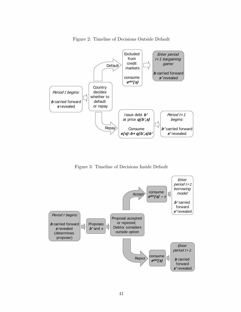
Figure 2: Timeline of Decisions Outside Default

Period t begins:

b carried forwards revealed

Excluded from credit

markets

consume edef(s)

Issue debt b’at price q(b’,s)

Consumee(s)-b+q(b’,s)b’

Enter period t+1 bargaining

game:

b carried forwards’ revealed

Period t+1 begins:

b’ carried forwards’ revealed

Country decides

whether to default or repay

Default

Repay

Figure 3: Timeline of Decisions Inside Default

Period t begins:

b carried forwards revealed

(determines proposer)

Proposesb’ and τ

Proposal accepted or rejected;

Debtor considersoutside option

Accept

Reject

consume edef(s) – τ

Enter period t+1:

b carried forward

s’ revealed

Enter period t+1borrowing

model:

b’ carried forward

s’ revealed

consume edef(s)

41

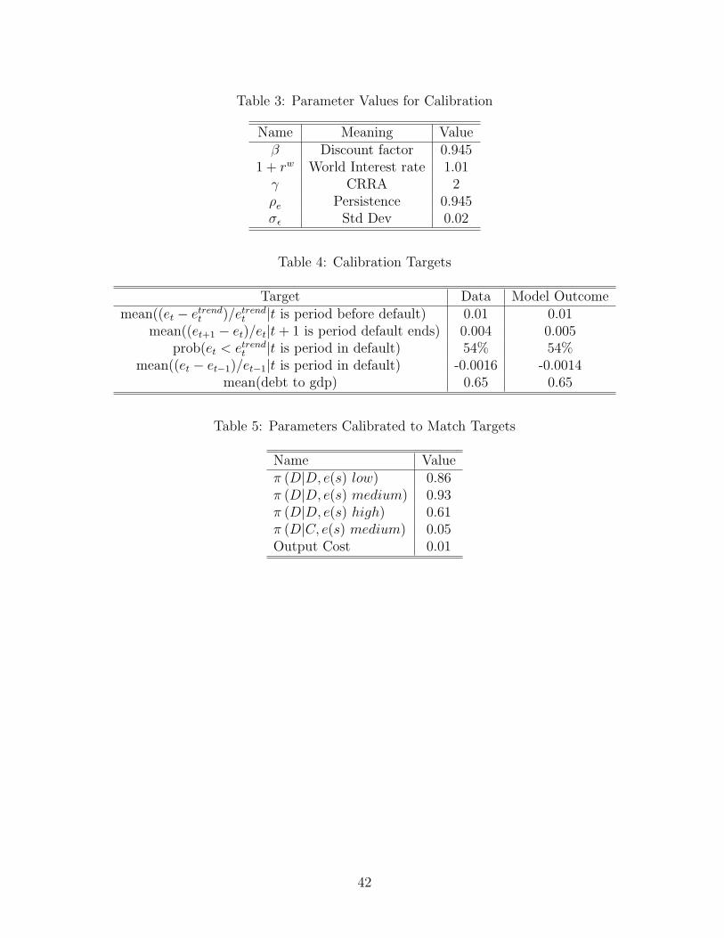
Table 3: Parameter Values for Calibration

Name Meaning Valueβ Discount factor 0.945

1 + rw World Interest rate 1.01γ CRRA 2ρe Persistence 0.945σε Std Dev 0.02

Table 4: Calibration Targets

Target Data Model Outcomemean((et − etrend

t )/etrendt |t is period before default) 0.01 0.01

mean((et+1 − et)/et|t + 1 is period default ends) 0.004 0.005prob(et < etrend

t |t is period in default) 54% 54%mean((et − et−1)/et−1|t is period in default) -0.0016 -0.0014

mean(debt to gdp) 0.65 0.65

Table 5: Parameters Calibrated to Match Targets

Name Valueπ (D|D, e(s) low) 0.86π (D|D, e(s) medium) 0.93π (D|D, e(s) high) 0.61π (D|C, e(s) medium) 0.05Output Cost 0.01

42

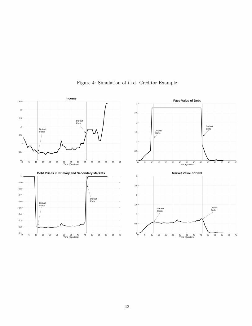
Figure 4: Simulation of i.i.d. Creditor Example

0 5 10 15 20 25 30 35 40 45 50 55 60 65 700

0.5

1

1.5

2

2.5

3

3.5

Time (Quarters)

Income

DefaultStarts

DefaultEnds

0 5 10 15 20 25 30 35 40 45 50 55 60 65 700

0.5

1

1.5

2

2.5

3

Time (Quarters)

Face Value of Debt

DefaultStarts

DefaultEnds

0 5 10 15 20 25 30 35 40 45 50 55 60 65 700.1

0.2

0.3

0.4

0.5

0.6

0.7

0.8

0.9

1

Time (Quarters)

Debt Prices in Primary and Secondary Markets

DefaultStarts

DefaultEnds

0 5 10 15 20 25 30 35 40 45 50 55 60 65 700

0.5

1

1.5

2

2.5

3

Time (Quarters)

Market Value of Debt

DefaultStarts

DefaultEnds

43

Figure 5: Equilibrium Objects in i.i.d. Creditor Example

0 0.5 1 1.5 2 2.5 3 3.5 40

0.1

0.2

0.3

0.4

0.5

0.6

0.7

0.8

0.9

1

Face Value of Debt

Default Probability (i.i.d. Creditor)

High IncomeLow IncomeMean Income

0 0.5 1 1.5 2 2.5 3 3.5 40

0.1

0.2

0.3

0.4

0.5

0.6

0.7

0.8

0.9

1

Face Value of Debt

Debt Prices (i.i.d. creditor)

High IncomeMean IncomeLow Income

0 0.5 1 1.5 2 2.5 3 3.5 40

0.1

0.2

0.3

0.4

0.5

0.6

0.7

0.8

0.9

1

Face Value of Debt

Market Value of Debt (i.i.d., Creditor)

Medium IncomeHigh IncomeLow Income

0 0.5 1 1.5 2 2.5 3 3.5 40

0.2

0.4

0.6

0.8

1

Face Value of Debt

Expected Value of Settlement (i.i.d. Creditor)

High IncomeLow IncomeMean Income

44

Figure 6: Simulation of Persistent Example

0 5 10 15 20 25 30 35 40 45 500.75

0.8

0.85

0.9

0.95

1

1.05

1.1

Time (Quarters)

Income

Begin outsidedefault, with creditoras proposer

Debtor becomesproposer; Default starts

Creditor becomesproposer; Default ends

0 5 10 15 20 25 30 35 40 45 500

0.2

0.4

0.6

0.8

1

1.2

1.4

1.6

1.8

2

Time (Quarters)

Face Value of Debt

Begin outsidedefault, with creditoras proposer

Debtor becomesproposer; Default starts

Creditor becomesproposer; Default ends

0 5 10 15 20 25 30 35 40 45 500

0.1

0.2

0.3

0.4

0.5

0.6

0.7

0.8

0.9

1

Time (Quarters)

Debt Prices in Primary and Secondary Markets

Begin outsidedefault, with creditoras proposer

Debtor becomesproposer; Default starts

Creditor becomesproposer; Default ends

0 5 10 15 20 25 30 35 40 45 500

0.2

0.4

0.6

0.8

1

1.2

1.4

1.6

1.8

2

Time (Quarters)

Market Value of Debt

Begin outsidedefault, with creditoras proposer

Debtor becomesproposer; Default starts

Creditor becomesproposer; Default ends

45

Figure 7: Equilibrium Objects in Persistent Example: Part I

0 0.5 1 1.5 2 2.5 30

0.1

0.2

0.3

0.4

0.5

0.6

0.7

0.8

0.9

1

Face Value of Debt

Default Probability (Persistent, Debtor Proposes)

High IncomeLow Income

0 0.5 1 1.5 2 2.5 30

0.1

0.2

0.3

0.4

0.5

0.6

0.7

0.8

0.9

1

Face Value of Debt

Default Probability (Persistent, Creditor Proposes)

High IncomeLow Income

0 0.5 1 1.5 2 2.5 30

0.1

0.2

0.3

0.4

0.5

0.6

0.7

0.8

0.9

1

Face Value of Debt

Debt Prices (Persistent, Debtor Proposes)

High IncomeLow Income

0 0.5 1 1.5 2 2.5 30

0.1

0.2

0.3

0.4

0.5

0.6

0.7

0.8

0.9

1

Face Value of Debt

Debt Prices (Persistent, Creditor Proposes)

High IncomeLow Income

46

Figure 8: Equilibrium Objects in Persistent Example: Part II

0 0.5 1 1.5 2 2.5 30

0.2

0.4

0.6

0.8

1

1.2

1.4

Face Value of Debt

Market Value of Debt (Persistent, Debtor Proposes)

Low IncomeHigh Income

0 0.5 1 1.5 2 2.5 30

0.2

0.4

0.6

0.8

1

1.2

1.4

Face Value of Debt

Market Value of Debt (Persistent, Creditor Proposes)

High IncomeLow Income

0 0.5 1 1.5 2 2.5 30

0.2

0.4

0.6

0.8

1

1.2

1.4

Face Value of Debt

Expected Value of Settlement (Persistent, Debtor Proposes)

High incomeLow Income

0 0.5 1 1.5 2 2.5 30

0.2

0.4

0.6

0.8

1

1.2

1.4

Face Value of Debt

Expected Value of Settlement (Persistent, Creditor Proposes)

Low IncomeHigh Income

47

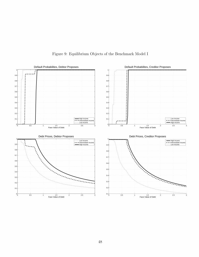
Figure 9: Equilibrium Objects of the Benchmark Model I

0 0.5 1 1.5 2 2.5 30

0.1

0.2

0.3

0.4

0.5

0.6

0.7

0.8

0.9

1

Face Value of Debt

Default Probabilites, Debtor Proposes

High IncomeIntermediate IncomeLow Income

0 0.5 1 1.5 2 2.5 30

0.1

0.2

0.3

0.4

0.5

0.6

0.7

0.8

0.9

1

Face Value of Debt

Default Probabilites, Creditor Proposes

Low IncomeIntermediate IncomeHigh Income

0 0.5 1 1.5 2 2.5 30

0.1

0.2

0.3

0.4

0.5

0.6

0.7

0.8

0.9

1

Face Value of Debt

Debt Prices, Debtor Proposes

Low IncomeIntermediate IncomeHigh Income

0 0.5 1 1.5 2 2.5 30.1

0.2

0.3

0.4

0.5

0.6

0.7

0.8

0.9

1

Face Value of Debt

Debt Prices, Creditor Proposes

High IncomeIntermediate IncomeLow Income

48

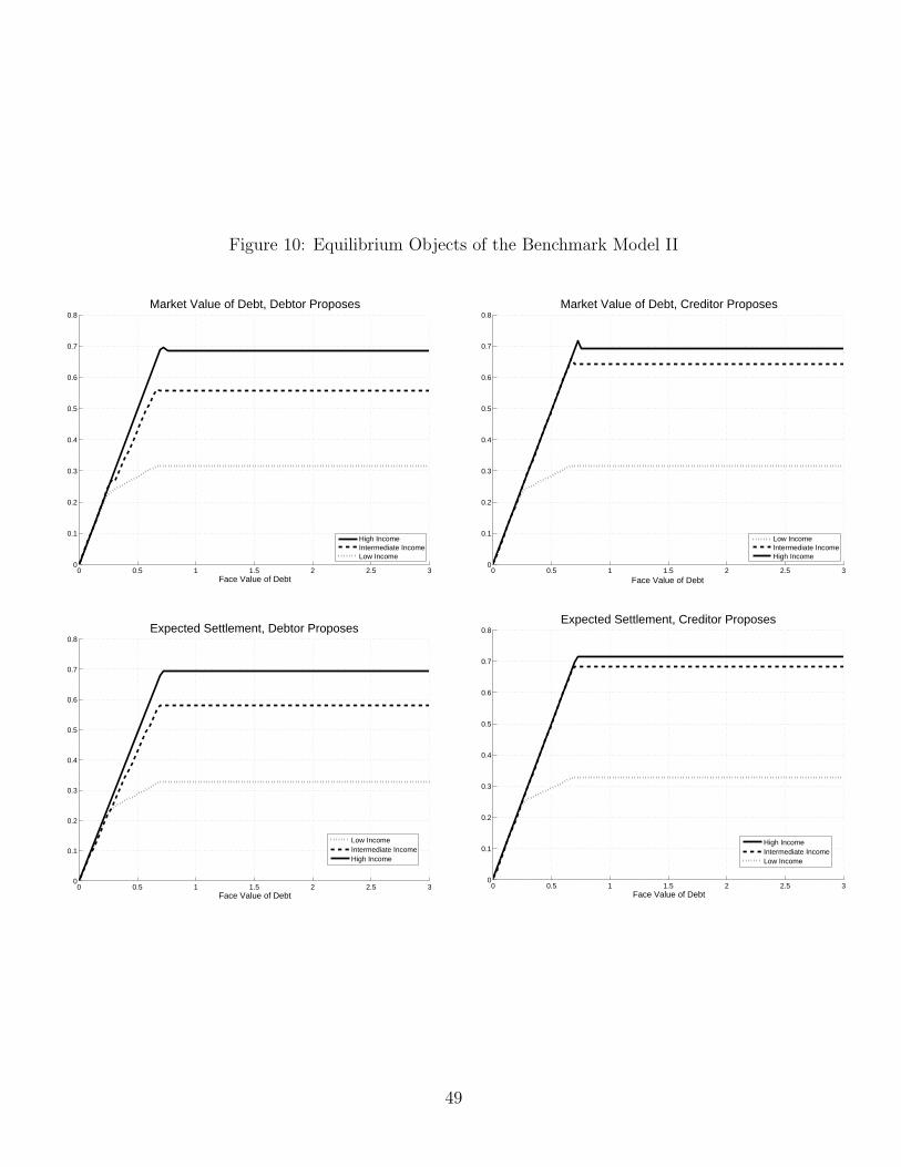
Figure 10: Equilibrium Objects of the Benchmark Model II

0 0.5 1 1.5 2 2.5 30

0.1

0.2

0.3

0.4

0.5

0.6

0.7

0.8

Face Value of Debt

Market Value of Debt, Debtor Proposes

High IncomeIntermediate IncomeLow Income

0 0.5 1 1.5 2 2.5 30

0.1

0.2

0.3

0.4

0.5

0.6

0.7

0.8Market Value of Debt, Creditor Proposes

Face Value of Debt

Low IncomeIntermediate IncomeHigh Income

0 0.5 1 1.5 2 2.5 30

0.1

0.2

0.3

0.4

0.5

0.6

0.7

0.8

Face Value of Debt

Expected Settlement, Debtor Proposes

Low IncomeIntermediate IncomeHigh Income

0 0.5 1 1.5 2 2.5 30

0.1

0.2

0.3

0.4

0.5

0.6

0.7

0.8

Face Value of Debt

Expected Settlement, Creditor Proposes

High IncomeIntermediate IncomeLow Income

49

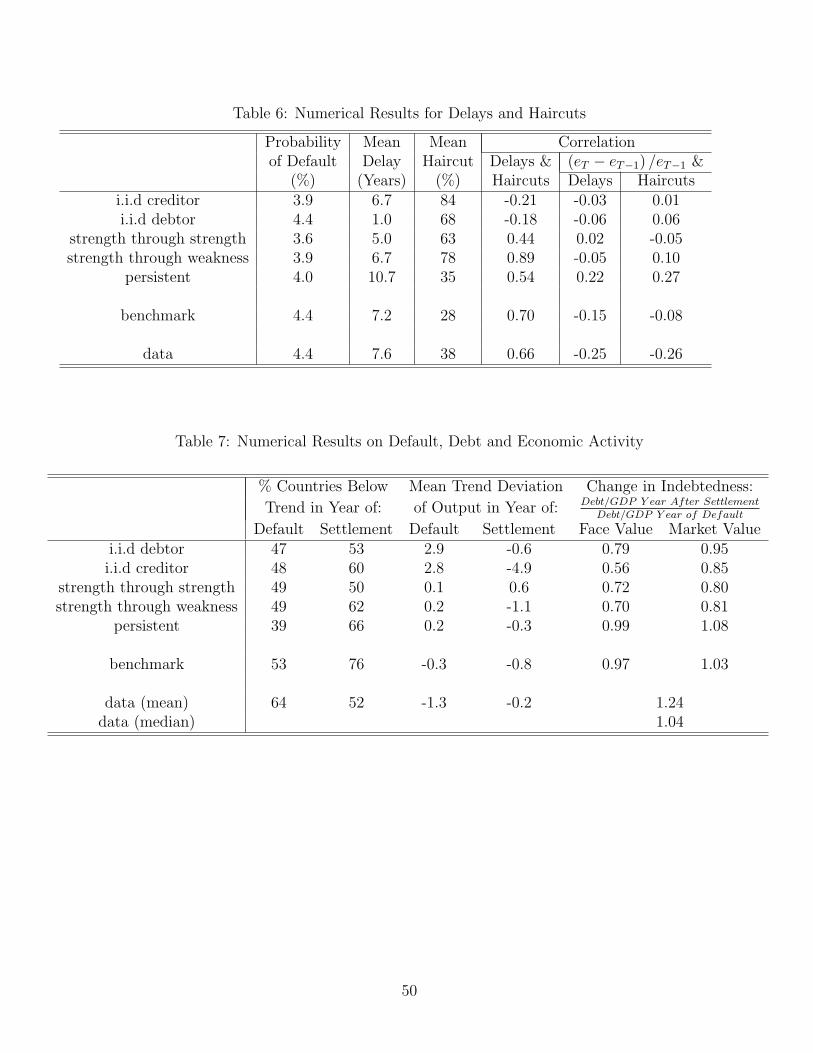
Table 6: Numerical Results for Delays and Haircuts

Probability Mean Mean Correlationof Default Delay Haircut Delays & (eT − eT−1) /eT−1 &

(%) (Years) (%) Haircuts Delays Haircutsi.i.d creditor 3.9 6.7 84 -0.21 -0.03 0.01i.i.d debtor 4.4 1.0 68 -0.18 -0.06 0.06

strength through strength 3.6 5.0 63 0.44 0.02 -0.05strength through weakness 3.9 6.7 78 0.89 -0.05 0.10

persistent 4.0 10.7 35 0.54 0.22 0.27

benchmark 4.4 7.2 28 0.70 -0.15 -0.08

data 4.4 7.6 38 0.66 -0.25 -0.26

Table 7: Numerical Results on Default, Debt and Economic Activity

% Countries Below Mean Trend Deviation Change in Indebtedness:

Trend in Year of: of Output in Year of: Debt/GDP Y ear After SettlementDebt/GDP Y ear of Default

Default Settlement Default Settlement Face Value Market Valuei.i.d debtor 47 53 2.9 -0.6 0.79 0.95i.i.d creditor 48 60 2.8 -4.9 0.56 0.85

strength through strength 49 50 0.1 0.6 0.72 0.80strength through weakness 49 62 0.2 -1.1 0.70 0.81

persistent 39 66 0.2 -0.3 0.99 1.08

benchmark 53 76 -0.3 -0.8 0.97 1.03

data (mean) 64 52 -1.3 -0.2 1.24data (median) 1.04

50

Table 8: Numerical Results on the Proportion of Countries Below Trend

RegimePeriod Before

DefaultPeriod OfDefault

Period OfSettlement

Period AfterSettlement

Quarterlyi.i.d debtor 97 99 87 84i.i.d creditor 99 97 52 56

strength through strength 1 5 42 40strength through weakness 98 99 57 53

persistent 60 89 89 58benchmark 46 90 73 19

Annuali.i.d debtor 4 47 53 86i.i.d creditor 3 48 60 55

strength through strength 96 49 50 40strength through weakness 3 49 62 40

persistent 15 39 66 62benchmark 25 53 76 29

data 40 64 52 49

Table 9: Numerical Results on Spreads, Income and Capital Flows: Quarterly Data

Correlation Between Face ValueModel Spreads & Income & Std Dev (C)/ of Debt/

NX/Y NX Income NX/Y NX Std Dev (Y) IncomeArellano (2007) 0.43 -0.29 -0.25 1.10 6Aguiar & Trend Stat -0.21 0.51 -0.33 0.99 27Gopinath (2007) Diff. Stat. 0.11 -0.03 -0.19 0.98 19Yue (2007) 0.54 -0.18 -0.14 1.03 10Bi (2008) -0.51 0.12 0.99 9

i.i.d debtor 0.23 -0.24 0.19 0.99 49i.i.d creditor 0.12 -0.45 0.27 0.98 246strength through strength 0.17 0.31 -0.20 1.27 51strength through weakness 0.19 -0.51 0.24 1.09 66persistent 0.25 -0.09 0.01 1.03 83

benchmark 0.32 -0.44 -0.24 1.09 69

data range min (abs. val.) 0.05 0.49 -0.12 -0.17 -0.64 1.03 65max (abs. val.) 0.86 0.70 -0.88 -0.89 -0.88 1.19

Sources: Arellano (2007) Tables 1 and 4. Aguiar and Gopinath (2007) Tables 1 and 3. Yue(2008) Table 4. Bi (2008) Table 4.

51

Figure 11: The Benefits of Bailouts: Low Output

-1 -0.8 -0.6 -0.4 -0.2 0-0.2

0

0.2

0.4Debtor Proposes, Inside Default

-1 -0.8 -0.6 -0.4 -0.2 0-0.2

0

0.2

0.4Creditor Proposes, Inside Default

-1 -0.8 -0.6 -0.4 -0.2 0-0.2

0

0.2

0.4Debtor Proposes, Outside Default

-1 -0.8 -0.6 -0.4 -0.2 0-0.2

0

0.2

0.4Creditor Proposes, Outside Default

Figure 12: The Costs of Bailouts: Low Output

-1 -0.8 -0.6 -0.4 -0.2 00.12

0.14

0.16

0.18

0.2Debtor Proposes, Inside Default

-1 -0.8 -0.6 -0.4 -0.2 00.12

0.14

0.16

0.18

0.2Creditor Proposes, Inside Default

-1 -0.8 -0.6 -0.4 -0.2 00.12

0.14

0.16

0.18

0.2Debtor Proposes, Outside Default

-1 -0.8 -0.6 -0.4 -0.2 00.12

0.14

0.16

0.18

0.2Creditor Proposes, Outside Default

52

Figure 13: The Benefits of Bailouts: Mean Output

-1 -0.8 -0.6 -0.4 -0.2 0-0.2

0

0.2

0.4Debtor Proposes, Inside Default

-1 -0.8 -0.6 -0.4 -0.2 0-0.2

0

0.2

0.4Creditor Proposes, Inside Default

-1 -0.8 -0.6 -0.4 -0.2 0-0.2

0

0.2

0.4Debtor Proposes, Outside Default

-1 -0.8 -0.6 -0.4 -0.2 0-0.2

0

0.2

0.4Creditor Proposes, Outside Default

Figure 14: The Costs of Bailouts: Mean Output

-1 -0.8 -0.6 -0.4 -0.2 00.12

0.14

0.16

0.18

0.2Debtor Proposes, Inside Default

-1 -0.8 -0.6 -0.4 -0.2 00.12

0.14

0.16

0.18

0.2Creditor Proposes, Inside Default

-1 -0.8 -0.6 -0.4 -0.2 00.12

0.14

0.16

0.18

0.2Debtor Proposes, Outside Default

-1 -0.8 -0.6 -0.4 -0.2 00.12

0.14

0.16

0.18

0.2Creditor Proposes, Outside Default

53

Table 10: The Effect of Bailouts

Benchmark Case

No Bailout BailoutLength of Default (years) 7.2 11.1

Time in Default (%) 44 75

Average Benefit(% lifetime consumption) -0.02

Average Cost(% lifetime consumption) 0.11

Average Net Benefit(% lifetime consumption) -0.13

Table 11: Probability of a Bailout

Sensitivity AnalysisProb of Bailout(per quarter) 0.00 0.05 0.10 0.15 0.20 0.25 0.30 0.35 0.40 0.45 0.50

Time inDefault (%) 44 43 74 75 75 75 100 96 100 100 100

Ave Net Benefit(% of life consn) 0.00 -0.04 -0.05 -0.11 -0.13 -0.10 -0.17 -0.15 -0.19 -0.20 -0.24

8 Appendix B: Proofs of Theorems

8.A Solution to the Bargaining Model

Recursive Problem StatementIn this section, we prove the equivalence between SSP payoffs and fixed points of the

T operator defined in the text. This requires some notation, and an intermediate Lemma.Take the SSP outcome, which consists of a set of states in which acceptance occurs

and the proposal that is accepted in that state, ((B × S)µ , µ) , as given. We can define thevalue of this outcome as follows. First, fix the value of the defaulted debt to b. Then, givena sequence of realizations of the state, define the stopping time for an agreement by t∗ where(b, st∗) ∈ (B × S)µ and (b, st) ∈ (B × S) \ (B × S)µ for all t = 0, ..., t∗−1. Then we can definethe value of this outcome in state s as

vµ (b, s) ≡(

vµ1 (b, s)

vµ2 (b, s)

)=

(E[∑t∗−1

t=0 βtU(edef (st

)+ βt∗

{U(edef (st∗)− τ (st∗)

)+ βV (b (st∗) , st∗)

}|s]

E[δt∗ {τ (st∗) + b (st∗) q (b (st∗) , st∗)} |s

] ).

First, we establish that the value function vµ (b, s) is the unique function defined on

54

B×S taking values in R2 satisfying a particular functional equation. The proof relies on thefollowing mapping which is defined for an arbitrary stationary outcome. Specifically, considerthe mapping T on the set of functions f : B × S → R2 into itself defined by:

Tf1(b, s) =

{u(edef (s)− τ (b, s)) + βE[V (b′ (b, s) , s′|s)] if (b, s) ∈ (B × S)µ

u(edef (s)) + βE [f1(b, s′)|s] if (b, s) ∈ (B × S) \ (B × S)µ ,

and

Tf2(b, s) =

{τ (b, s) + b′ (b, s) q(b′ (b, s) , s) if (b, s) ∈ (B × S)µ

δE[f2(b, s′)|s] if (b, s) ∈ (B × S) \ (B × S)µ .

The first operator applies to the payoff of the debtor country, and simply states that if (b, s)is in the set (B × S)µ , which is the set of debt levels and states in which either the outsideoption is taken or a proposal is accepted, then the payoff to the country is found by evaluatingthe value of that proposal. Conversely, if (b, s) is not in the acceptance set, the debtor countryconsumes its endowment in default today and the discounted value of the expected payofffrom continuing the bargaining game tomorrow. The second operator is similar and appliesto the payoff of the creditors.

Lemma B. 1. Given an outcome ((B × S)µ , µ) where µ = (τ , b), vµ is the unique functiondefined on B × S taking values in R2 for which

(vµ

1 (b, s)vµ

2 (b, s)

)=

(

u(edef (s)− τ (b, s)) + βE[V (b′ (b, s) , s′)|s]τ (b, s) + b′ (b, s) q (b′ (b, s) , s) if s ∈ Sµ

)(

u(edef (s)) + βE [vµ1 (b, s′)|s]

δE[vµ2 (b, s′)|s] if s ∈ S\Sµ

) .

Proof. The proof requires us to show that vµ is a fixed point of the operator T, and thatthe operator T has a unique fixed point. First, to see that vµ is a fixed point, note that if(b, s0) ∈ (B × S)µ then

Tvµ (b, s0) =

(u(edef (s0)− τ (b, s0)) + βE[V (b′ (b, s0) , s1|s0)]

τ (b, s0) + b′ (b, s0) q(b′ (b, s0) , s0)

),

which is precisely the definition of vµ on states for realizations in which the stopping time iszero. Alternatively, suppose that (b, s0) ∈ (B × S) \ (B × S)µ. Then by definition of T wehave

T

(vµ

1 (b, s0)vµ

2 (b, s0)

)=

(u(edef (s0)) + βE[vµ

1 (b, s1)|s0]δE[vµ

2 (b, s1)|s0]

).

Define a stopping time t∗,such that if (b, s0) is the initial state, t∗ is the period in whichagreement is reached. That is, (b, st∗) ∈ (B × S)µ and (b, st) ∈ (B × S) \ (B × S)µ for all

55

t < t∗. Then iterating on the operator T we have

T

(vµ

1 (b, s0)vµ

2 (b, s0)

)=

(u(edef (s0)) + βE[vµ

1 (b, s1)|s0]δE[vµ

2 (b, s1)|s0]

)=

(u(edef (s0)) + βE[

∑t∗−1t=1 βtu

(edef (st)

)+ βt∗E[vµ

1 (b, st∗) |s1]|s0]δ[E[E[δt∗vµ

2 (b, st∗)|s1]]|s0

] )=

(E[∑t∗−1

t=0 βtU(edef (st)

)+ βt∗

{U(edef (st∗)− τ (b, st∗)

)V (b′ (b, st∗) , st∗)

}|s]

E[δt∗ {τ (b, st∗) + b′ (b, st∗) q (b′ (b, st∗) , st∗)} |s

] )= vµ.

Second, to show that T has a unique fixed point it is sufficient to show that T is acontraction on the metric space of functions defined on B × S taking values in R2 endowedwith the sup (or in this case, the max) norm. That is, we require that if f 1 and f 2 are eachfunctions mapping B × S into R2, then

||T (f 1)− T (f 2)||∞ ≤ δ||f 1 − f 2||∞.

To see this, note that if (b, s) ∈ (B × S)µ , then Tf is independent of the function f andhence∣∣Tf 1 (b, s)− Tf 2 (b, s)

∣∣ = max{∣∣Tf 1

1 (b, s)− Tf 21 (b, s)

∣∣ , ∣∣Tf 12 (b, s)− Tf 2

2 (b, s)∣∣} = 0.

Otherwise, ∣∣Tf 1(b, s)− Tf 2(b, s)∣∣

= max{∣∣βE[f 1

1 (b, s′)|s]− βE[f 21 (b, s′)|s]

∣∣ , ∣∣δE[f 12 (b, s′)|s]− δE[f 2

2 (b, s′)|s]∣∣}

= β max{∣∣E[f 1

1 (s′)− f 21 (s′)|s]

∣∣ , ∣∣E[f 12 (s′)− f 2

2 (s′)|s]∣∣}

≤ β||f 1 − f 2||∞,

where we have exploited our assumption that β < δ < 1. But then∥∥Tf 1 − Tf 2∥∥∞ = max

b,s

∣∣Tf 1 (b, s)− Tf 2 (b, s)∣∣ ≤ β||f 1 − f 2||∞.

Using the result of the previous Lemma, the following theorem establishes an equiva-lence between SSP payoffs and fixed points of the T operator.

Theorem 1. The functions f = (f1, f2) are SSP payoffs if and only if T f = f.

Proof. First, suppose that f are SSP payoffs. Fix (b, s) ∈ B × S. Suppose that no proposalis accepted at (b, s) , and the outside option is not taken. Then the SSP payoffs f satisfy therelationships

f1 (b, s) = u(edef (s)) + βE [f1(b, s′)|s] ,

f2 (b, s) = δE [f2(b, s′)|s] .

56

If a proposal is accepted at (b, s) , it must be that it gives the agent who receives theproposal at least their reservation utility. If the debtor is proposing, then it must be thatthe proposal (τ , b′) satisfies

τ + b′q(b′, s) ≥ min {b, δE[f2(b, s′)|s]} = δE[f2(b, s

′)|s],

while if the creditor is proposing, it must satisfy

u(edef − τ) + βE[V (b′, s′)|s]

≥ max

{u(edef (s)) + βE [f1(b, s

′)|s] , maxτ,b′ u(edef (s)− τ) + βE[V (b′, s′)|s]s.t τ + b′q(b′, s) ≥ b

}.

Moreover, as the proposal is part of a SSP, it must give the proposer the largest payoffover all such feasible proposals. Hence, if the debtor proposes in a state where a proposal isaccepted

f1 (b, s) = maxτ,b′

u(edef (s)− τ) + βE[V (b, s′)|s],

s.t. τ + b′q(b′, s) ≥ min {b, δE[f2(b, s′)|s]} ,

while if a creditor proposes, it must be that

f2 (b, s) = min

{b,

maxτ,b′ τ + b′q(b′, s),s.t. u(edef (s)− τ) + βE[V (b′, s′)|s] ≥ u(edef (s)) + βE [f1(b, s

′)|s]

}.

Finally, as the proposer can always guarantee themselves their reservation payoff (or theoutside option in the case of the debtor) by proposing something that will not be accepted,it must be that

f1(b, s) = max

{maxτ,b′ u(edef (s)− τ) + βE[V (b′, s′)|s]

s.t τ + b′q(b′, s) ≥ min {b, δE[f2(b, s′)|s]} , u(edef (s)) + βE [f1(b, s

′)|s]}

when the debtor proposes, and

f2(b, s) = max

{min

{b,

maxτ,b′ τ + b′q(b′, s)s.t u(edef (s)− τ) + βE[V (b′, s′)|s] ≥ u(edef (s)) + βE [f1(b, s

′)|s]

}, δE [f2(b, s

′)|s]}

when the creditor proposes. But then T f = f.Second, suppose that T f = f. We will construct a SSP outcome ((B × S)µ , µ) for

which f = vµ. We construct (B × S)µ by noting that, if for a given (b, s) there exists (τ , b′)such that

f1 (b, s) = u(edef (s)− τ) + βE[V (b′, s′)|s]f2(b, s) = τ + b′q(b′, s),

then (b, s) is an agreement state and hence (b, s) ∈ (B × S)µ . Then for that state we let

µ (b, s) = (τ , b′) .

Otherwise, we say (b, s) ∈ (B × S) \ (B × S)µ .

57

We need to show that the value of the outcome ((B × S)µ , µ) , vµ, is equal to f andthat it is a SSP outcome. To show that the value of the outcome is vµ, consider any state(b, s) . Since T f = f, for the non-proposing player we have

f1(b, s) = u(edef (s)) + βE [f1(b, s′)|s] ,

f2(b, s) = min {b, δE [f2(b, s′)|s]} ,

while for the proposing country we have

T f1(b, s) = max

{maxτ,b′ u(edef (s)− τ) + βE[V (b′, s′)|s]

s.t τ + b′q(b′, s) ≥ δE[f2(b, s′)|s] , u(edef (s)) + βE [f1(b, s

′)|s]}

,

with an analogous result for the creditor. If τ + b′q(b′, s) = f2(b, s), then (b, s) ∈ (B × S)µ

by construction andf1 (b, s) = u(edef (s)− τ) + βE[V (b′, s′)|s].

If τ + b′q(b′, s) < f2(b, s), then (b, s) /∈ (B × S)µ and

f1 (b, s) = u(edef (s)) + βE [f1(b, s′)|s] .

but in Lemma 1 we showed that vµ was the unique function satisfying these conditions.Hence f = vµ.

Finally, to show that ((B × S)µ , µ) is a SSP outcome, consider a strategy designedas follows: (i) if (b, s) ∈ (B × S)µ , then propose µ (b, s) , otherwise propose an outcome thatdelivers the other player strictly less than vµ (b, s) ; (ii) accept any proposal as long as itdelivers at least vµ (b, s) . To see that this is a subgame perfect equilibrium, consider a nodeat which a player has yet to propose. µ (b, s) delivers at least vµ (b, s) by the previous result

and so will be accepted. Moreover, as T vµ = vµ, this proposal maximizes the payoff of theproposer subject to delivering this utility level. Hence a proposer cannot gain by deviatingto any other proposal. Next, consider a node at which a proposal has been made. If theproposal gives strictly less than vµ (b, s) , the player can only lose by accepting it. If theproposal gives exactly vµ (s) , then by construction it also delivers exactly the reservationpayoff of the agent, which is the value they expect from rejecting the offer. Hence, a onestage rejection of a proposal gives the same expected payoff. Familiar arguments show thatby iterating on this argument we can rule out finite stage deviations, while boundedness anddiscounting rule out infinite deviations.

Existence and Uniqueness of SSP Equilibria of the Bargaining ModelNext we show that an SSP equilibrium exists, and provide a condition under which

the SSP equilibrium is unique. Existence is proven by demonstrating that our T mappingoperates on a bounded set of functions, and is monotone. Let F (B × S) be the space of allfunctions mapping B×S into R2, and let B (B × S) be the subset of F (B × S) that satisfiesthe following bounds

mins∈S

u(edef (s)

)1− δ

≡ Vmin ≤ min(b,s)∈B×S

f1 (b, s) ≤ max(b,s)∈B×S

f1 (b, s)

≤ Vmax ≡ max(b,s,s′)∈B×S×S

u (e (s)− b) + βV (b, s′) ,

bmin ≡ min B ≤ min(b,s)∈B×S

f2 (b, s) ≤ max(b,s)∈B×S

f2 (b, s) ≤ bmax ≡ max B.

58

We endow B (B × S) with the supremum (in this case, maximum) norm.

Lemma B. 2. The operator T maps B (B × S) into itself.

Proof. To see that if f ∈ B (B × S) then T f ∈ B (B × S) , first consider the creditors con-tinuation value function. Fix b. Then if s is such that the debtor proposes

T2(f1, f2) (b, s) = min {b, δE [f2 (b, s′) |s]} ∈ [bmin, bmax] .

If s is such that the creditor proposes

T2 (f1, f2) (b, s) = max

min

b,maxτ,b′ τ + b′q(b′, s)

s.t u(edef (s)− τ) + βE[V (b′, s′)|s]≥ u(edef (s)) + βE [f1(b, s

′)|s]

, δE [f2(b, s′)|s]

≤ max {b, δE [f2(b, s

′)|s]} ≤ bmax,

and

T2 (f1, f2) (b, s) = max

min

b,maxτ,b′ τ + b′q(b′, s)

s.t u(edef (s)− τ) + βE[V (b′, s′)|s]≥ u(edef (s)) + βE [f1(b, s

′)|s]

, δE [f2(b, s′)|s]

≥ δE [f2(b, s

′)|s] ≥ bmin,

since bmin ≤ 0.Next consider the debtor’s continuation value function. Fix b. Then if s is such that

the creditor proposes

T1 (f1, f2) (b, s)

= max

{u(edef (s)

)+ βE [f1 (b, s′) |s] , maxτ,b′ u

(edef (s)− τ

)+ βE [V (b′, s′) |s]

s.t τ + b′q (b′, s) ≥ b

}≤ max

{u(edef (s)− bmin

)+ βVmax, Vmax

}≤ Vmax,

and

T1 (f1, f2) (b, s) = max

{u(edef (s)

)+ βE [f1 (b, s′) |s] , maxτ,b′ u

(edef (s)− τ

)+ βE [V (b′, s′) |s]

s.t τ + b′q (b′, s) ≥ b

}≥ u

(edef (s)

)+ βE [f1 (b, s′) |s] ≥ Vmin.

If s is such that the debtor proposes

T1 (f1, f2) (b, s)

= max

{maxτ,b′ u(edef (s)− τ) + βE[V (b′, s′)|s]

s.t τ + b′q(b′, s) ≥ min {b, δE [f2 (b, s′) |s]} ,, u(edef (s)) + βE [f1(b, s

′)|s]}

≥ u(edef (s)) + βE [f1(b, s′)|s] ≥ Vmin,

59

and

T1 (f1, f2) (b, s)

= max

{maxτ,b′ u(edef (s)− τ) + βE[V (b′, s′)|s]

s.t τ + b′q(b′, s) ≥ min {b, δE [f2 (b, s′) |s]} ,, u(edef (s)) + βE [f1(b, s

′)|s]}

≤ max{Vmax, u

(edef (s)− bmin

)+ βVmax

}≤ Vmax.

Lemma B. 3. The operator T is monotone. That is, if there exists functions f1, f′1, f2, f

′2 ∈

F (B × S) such that f1 > f ′1 and f ′2 > f2 then

T1(f1, f2) ≥ T1(f′1, f

′2) and T2(f1, f2) ≤ T2(f

′1, f

′2).

Proof. Take the functions f1, f′1, f2, f

′2 as given. Fix b and consider a state s in which the

debtor proposes. Then it follows immediately that the creditor’s value satisfies

T2(f1, f2) (b, s) = min {b, δE [f2 (b, s′) |s]} ≤ min {b, δE [f ′2 (b, s′) |s]} = T2(f′1, f

′2) (b, s) .

For the debtor’s value, we have

T1 (f1, f2) (b, s)

= max

{maxτ,b′ u(edef (s)− τ) + βE[V (b′, s′)|s]

s.t τ + b′q(b′, s) ≥ min {b, δE [f2 (b, s′) |s]} ,, u(edef (s)) + βE [f1(b, s

′)|s]}

≥ max

{maxτ,b′ u(edef (s)− τ) + βE[V (b′, s′)|s]

s.t τ + b′q(b′, s) ≥ min {b, δE [f ′2 (b, s′) |s]} ,, u(edef (s)) + βE [f ′1(b, s

′)|s]}

= T1(f′1, f

′2) (b, s) .

As this is true for all (b, s) , monotonicity holds for this region of the state space.Now consider s such that the creditor proposes. The debtor’s value satisfies

T1 (f1, f2) (b, s)

= max

{u(edef (s)

)+ βE [f1 (b, s′) |s] , maxτ,b′ u

(edef (s)− τ

)+ βE [V (b′, s′) |s]

s.t τ + b′q (b′, s) ≥ b

}≥ max

{u(edef (s)

)+ βE [f ′1 (b, s′) |s] , maxτ,b′ u

(edef (s)− τ

)+ βE [V (b′, s′) |s]

s.t τ + b′q (b′, s) ≥ b

}= T2 (f ′1, f

′2) (b, s) .

60

Similarly, the creditor’s value satisfies

T2 (f1, f2) (b, s)

= max

min

b,maxτ,b′ τ + b′q(b′, s)

s.t u(edef (s)− τ) + βE[V (b′, s′)|s]≥ u(edef (s)) + βE [f1(b, s

′)|s]

, δE [f2(b, s′)|s]

≤ max

min

b,maxτ,b′ τ + b′q(b′, s)

s.t u(edef (s)− τ) + βE[V (b′, s′)|s]≥ u(edef (s)) + βE [f1(b, s

′)|s]

, δE [f ′2(b, s′)|s]

≤ max

min

b,maxτ,b′ τ + b′q(b′, s)

s.t u(edef (s)− τ) + βE[V (b′, s′)|s]≥ u(edef (s)) + βE [f ′1(b, s

′)|s]

, δE [f ′2(b, s′)|s]

= T2 (f ′1, f

′2) (b, s) ,

where the last inequality comes from the fact that f ′1 ≤ f1 which loosens the constraint onthe creditor’s maximization problem and thus weakly increases the value of the program.

The proof of existence then follows by applying the T operator to a suitable initial f 0 withinthe space B (B × S).

Theorem 2. An SSP equilbrium exists.

Proof. Choose f 0 = (f 01 , f0

2 ) such that for all (b, s) , f01 (b, s) = Vmax and f 0

2 (b, s) = bminand

successively apply the operator T to obtain the sequence of functions {fn}∞n=0 where fn+1 =

T fn. By Lemma 4 T is monotone, and by Lemma 3 T maps B (B × S) into itself, so thatthis is a monotone sequence of functions in B (B × S). Hence, the sequence converges to aSSP equilibrium values and by Theorem 2 and Lemma 1 there exists a SSP equilibrium.

The following theorem provides bounds on the rate at which resources can be trans-formed into utility, and the rate at which utility can be transformed into resources which, ifsatisfied, are sufficient to establish uniqueness of this fixed point.

Theorem 3. Let u : R → R be differentiable. If there exists KL > β and KU < 1/δ suchthat KL ≤ u′ (c) ≤ KU , for all c, then the SSP equilibrium values are unique.

Proof. Let f 1 = (f 11 , f1

2 ) and f 2 = (f 21 , f2

2 ) be elements of B (B × S). To establish the result,we need to show that there exists a γ ∈ (0, 1) such that

||T f 1 − T f 2||∞= max

(b,s)∈B×S

{max

{∣∣∣(T f 11

)(b, s)−

(T f 2

1

)(b, s)

∣∣∣ , ∣∣∣(T f 12

)(b, s)−

(T f 2

2

)(b, s)

∣∣∣}}≤ γ max

(b,s)∈B×S

{max

{∣∣f 11 (b, s)− f 2

1 (b, s)∣∣ , ∣∣f 1

2 (b, s)− f 22 (b, s)

∣∣}}≤ γ||f 1 − f 2||∞.

61

The argument varies according to whether the outside offer is taken, no proposal is accepted,or a proposal is accepted.

First, fix (b, s) and consider the case in which s is such that the debtor proposes. Ifthe outside option is taken for both f 1 and f 2, then we have∣∣∣(T f 1

)(b, s)−

(T f 2

)(b, s)

∣∣∣ = 0,

since the creditor’s payoff is b, and the debtor’s payoff solves

maxτ,b′ u(edef (s)− τ) + βE[V (b′, s′)|s]s.t τ + b′q(b′, s) ≥ b,

neither or which depends on the continuation values f 1 and f 2.If no proposal is accepted for both f 1 and f 2, then we have∣∣∣(T f 1

2

)(b, s)−

(T f 2

2

)(b, s)

∣∣∣ =∣∣δE [f 1

2 (b, s′) |s]− δE

[f 2

2 (b, s′) |s]∣∣ ≤ δ||f 1

2 − f 22 ||∞,

for the creditor’s continuation value function, and∣∣∣(T f 11

)(b, s)−

(T f 2

1

)(b, s)

∣∣∣=

∣∣u(edef (s)) + βE [f1(b, s′)|s]− u(edef (s))− βE [f1(b, s

′)|s]∣∣

= β |E [f1(b, s′)|s]− E [f1(b, s

′)|s]|≤ β

∥∥f 11 − f 2

1

∥∥∞ .

for the debtor’s continuation value function.If a proposal is accepted for both f 1 and f 2, consider first the case in which s is such

that the debtor proposes. In this case, the creditor’s continuation values satisfy∣∣∣(T f 12

)(b, s)−

(T f 2

2

)(b, s)

∣∣∣ =∣∣δE [f 1

2 (b, s′) |s]− δE

[f 2

2 (b, s′) |s]∣∣ ≤ δ||f 1

2 − f 22 ||∞.

Using this fact, the debtor’s continuation values satisfy∣∣∣(T f 11

)(b, s)−

(T f 2

1

)(b, s)

∣∣∣=

∣∣∣∣ maxτ,b′ u(edef (s)− τ

)+ βE [V (b′, s′) |s]

s.t τ + b′q (b′, s) ≥ δE [f 12 (b, s′) |s]

− maxτ,b′ u(edef (s)− τ

)+ βE [V (b′, s′) |s]

s.t τ + b′q (b′, s) ≥ δE [f 22 (b, s′) |s]

∣∣∣∣≤

∣∣∣∣ maxτ,b′ u(edef (s)− τ

)+ βE [V (b′, s′) |s]

s.t τ + b′q (b′, s) ≥ δE [f 22 (b, s′) |s] + δ||f 1

2 − f 22 ||∞

− maxτ,b′ u(edef (s)− τ

)+ βE [V (b′, s′) |s]

s.t τ + b′q (b′, s) ≥ δE [f 22 (b, s′) |s]

∣∣∣∣ .Now suppose that (τ 2, b′2) attain the maximum for f 2

2 . Then exploiting the fact that U isdefined over negative consumptions and that its slope is bounded we can find a feasible τ

62

such thatτ = τ 2 + δ

∥∥f 12 − f 2

2

∥∥∞ ,

yielding ∣∣∣(T f 11

)(b, s)−

(T f 2

1

)(b, s)

∣∣∣≤

∣∣u (edef (s)− τ 2 + δ∥∥f 1

2 − f 22

∥∥∞

)+ βE

[V(b2, s′

)|s]− u

(edef (s)− τ 2

)−βE

[V(b2, s′

)|s]∣∣

≤∣∣u (edef (s)− τ 2

)+ u′

(edef (s)− τ 2

)δ∥∥f 1

2 − f 22

∥∥∞ − u

(edef (s)− τ 2

)∣∣≤ δKU

∥∥f 12 − f 2

2

∥∥∞ .

Next consider the case in which s is such that the creditor proposes. In this case, thedebtor’s continuation values satisfy∣∣∣(T f 1

1

)(b, s)−

(T f 2

1

)(b, s)

∣∣∣=

∣∣βE[f 1

1 (b, s′) |s]− βE

[f 2

1 (b, s′) |s]∣∣ ≤ β||f 1

1 − f 21 ||∞.

Using this fact, the creditor’s continuation values satisfy∣∣∣(T f 12

)(b, s)−

(T f 2

2

)(b, s)

∣∣∣=

∣∣∣∣∣∣maxτ,b′ τ + b′q(b′, s)

s.t u(edef (s)− τ) + βE[V (b′, s′)|s]≥ u(edef (s)) + βE [f 1

1 (b, s′)|s]−

maxτ,b′ τ + b′q(b′, s)s.t u(edef (s)− τ) + βE[V (b′, s′)|s]≥ u(edef (s)) + βE [f 2

1 (b, s′)|s]

∣∣∣∣∣∣≤

∣∣∣∣∣∣maxτ,b′ τ + b′q(b′, s)

s.t u(edef (s)− τ) + βE[V (b′, s′)|s]≥ u(edef (s)) + βE [f 1

1 (b, s′)|s]

−maxτ,b′ τ + b′q(b′, s)

s.t u(edef (s)− τ) + βE[V (b′, s′)|s]≥ u(edef (s)) + βE [f 1

1 (b, s′)|s] + β ‖f 11 − f 2

1‖∞

∣∣∣∣∣∣ .Now suppose that (τ 1, b′1) attain the maximum for f 1

1 . Then there exists a τ such that∣∣τ − τ 1∣∣ ≤ βKL

∥∥f 11 − f 2

1

∥∥∞ ,

and that (τ , b′2) is feasible for f 11 and so∣∣∣(T f 1

2

)(b, s)−

(T f 2

2

)(b, s)

∣∣∣ ≤ β1

KL

∥∥f 11 − f 2

1

∥∥∞ .

It remains to consider cases that involve combinations of the outside option, no pro-posal being accepted, and a proposal being accepted. Suppose the outside option is takenfor one of the f i and no proposal is accepted for f−i. The argument is analogous regardlessof whether the debtor proposes or the creditor proposes at s. Without loss of generality we

63

can order the creditor’s continuation value functions such that∣∣∣(T f 12

)(b, s)−

(T f 2

2

)(b, s)

∣∣∣ =∣∣b− δE

[f 2

2 (b, s′) |s]∣∣

≤∣∣δE [f 1

2 (b, s′) |s]− δE

[f 2

2 (b, s′) |s]∣∣

≤ δ||f 12 − f 2

2 ||∞,

while for the debtor, if we define

V oo (b, s) =maxτ,b′ u(edef (s)− τ) + βE[V (b′, s′)|s]

s.t τ + b′q(b′, s) ≥ b,

we have ∣∣∣(T f 11

)(b, s)−

(T f 2

1

)(b, s)

∣∣∣=

∣∣V oo (b, s)− u(edef (s)) + βE[f 2

1 (b, s′)|s]∣∣

≤∣∣u (edef (s)

)+ βE

[f 2

1 (b, s′) |s]− u(edef (s))− βE

[f 1

1 (b, s′)|s]∣∣

≤ β∥∥f 1

1 − f 21

∥∥∞ .

where the first inequality follows from the fact that the debtor did not take the outside optionfor f 2 and the fact that the value of the outside option is independent of the continuationvalues.

Now suppose the outside option is taken for one of the f i and a proposal is acceptedfor f−i. If s is such that the debtor proposes, then the argument for the creditor is the sameas in the previous case since they earn their autarky value from an accepted proposal. Forthe debtor, we have∣∣∣(T f 1

1

)(b, s)−

(T f 2

1

)(b, s)

∣∣∣=

∣∣∣∣ maxτ,b′ u(edef (s)− τ

)+ βE [V (b′, s′) |s]

s.t τ + b′q (b′, s) ≥ δE [f 12 (b, s′) |s] − V oo (b, s)

∣∣∣∣≤

∣∣∣∣ maxτ,b′ u(edef (s)− τ

)+ βE [V (b′, s′) |s]

s.t τ + b′q (b′, s) ≥ δE [f 12 (b, s′) |s] − maxτ,b′ u

(edef (s)− τ

)+ βE [V (b′, s′) |s]

s.t τ + b′q (b′, s) ≥ δE [f 22 (b, s′) |s]

∣∣∣∣≤ δKU

∥∥f 12 − f 2

2

∥∥∞ ,

where the first inequality follows from the fact that the debtor did not take the outside optionfor f 2. If s is such that the creditor proposes, the argument for the debtor’s continuationvalue function is the same as in the previous case because the debtor receives their autarkyvalue from an accepted proposal. For the creditor, the result follows from an argumentsimilar to the debtor proposer case.

Finally, consider the case where no agreement occurs for f 1 and an agreement occursfor f 2. Non-proposers receive their autarky values in both cases, implying no differencein continuation value functions under the T operator. For the proposer, the fact that noagreement is chosen over agreement for f 2 means we can apply the same argument as in theprevious case.

Since the result holds for arbitrary (b, s) , the operator T is a contraction with modulus

γ = max {δ, β, δKU , β/KL} .

64

8.B Solution to the Borrowing Problem

In this subsection, we prove the following theorem:

Theorem 4. Given(V D (b, s) , W (b, s)

)∈ B (B × S) and q (b, s) ∈ Q (B × S) , there exists

a value function for the country, V (b, s) , and an equilibrium bond price function q (b, s) ∈Q (B × S) , that solve the borrowing problem.

The proof proceeds by establishing the following two Lemmata. The first takes thebond price function as given and establishes the existence of a unique solution to the country’sproblem.

Lemma B. 4. Given(V D (b, s) , W (b, s)

)∈ B (B × S) and q (b, s) ∈ Q (B × S) , there exists

a unique solution to the country’s borrowing problem, V (b, s) .

Proof. Let G (B × S) be the space of all real functions on B×S, bounded below by V D (b, s) ,and above by U (maxs∈S e (s)− bmax + bmin/ (1 + rw)) / (1− β) . It is straightforward to showthat T V maps G (B × S) into itself.

For any f ∈ G (B × S) define the operator T V by

(T V f

)(b, s) = max

{maxc,b′∈B U (c) + β

∑s′∈S π (s′|s) f (b′, s′) ,

s.t. c− q (b′, s) b′ ≤ e (s) + b., V D (b, s)

}.

First, we show that the operator T V is monotone. Let f 1, f2 ∈ G (B × S) such that f 1 ≥ f 2.Then for all (b, s)

(T V f 1

)(b, s) = max

{maxc,b′∈B U (c) + β

∑s′∈S π (s′|s) f 1 (b′, s′) ,

s.t. c− q (b′, s) b′ ≤ e (s) + b., V D (b, s)

}≥ max

{maxc,b′∈B U (c) + β

∑s′∈S π (s′|s) f 2 (b′, s′) ,

s.t. c− q (b′, s) b′ ≤ e (s) + b., V D (b, s)

}≥

(T V f 2

)(b, s) .

Next, we show that the operator T V satisfies the discounting property. Let a ∈ R.Then for all f ∈ G (B × S) and all (b, s) we have∣∣T V (f + a) (b, s)− T V (f) (b, s)

∣∣=

∣∣∣∣max

{maxc,b′∈B U (c) + β

∑s′∈S π (s′|s) f (b′, s′) + βa

s.t. c− q (b′, s) b′ ≤ e (s) + b, V D (b, s)

}− T V (f) (b, s)

∣∣∣∣≤

∣∣∣∣max

{maxc,b′∈B U (c) + β

∑s′∈S π (s′|s) f (b′, s′)

s.t. c− q (b′, s) b′ ≤ e (s) + b, V D (b, s)

}+ βa− T V (f) (b, s)

∣∣∣∣= βa.

Hence, T V is a contraction with modulus β, and there exists a unique fixed point inG (B × S) .

The second Lemma constructs a new operator and shows that, in combination withthe result of the first Lemma, that the composition of these operators is monotone, and hencethat an equilibrium exists.

65

Lemma B. 5. Given(V D (b, s) , W (b, s)

)∈ B (B × S) , there exists an equilibrium bond

price function q (b, s) ∈ Q (B × S) .

Proof. For any gn ∈ Q (B × S) , define the operator T q as follows. First, given gn, apply theoperator T V (which is defined for a given g) until convergence to V n with associated

(V R)n

.Then define

φn (b, s) =

{1 if V D (b, s) >

(V R)n

(b, s)

0 if V D (b, s) ≤(V R)n

(b, s),

which embodies the behavioral assumption that when indifferent between default and repay-ment the country always repays, from which can be constructed the default probability

pn (b, s) =∑

b∈B,s′∈S

φn (b, s′) π (s′|s) ,

and a new bond price function

gn (b, s) =1− p (b, s) + p (b, s)

∑s′∈S π (s′|s) W (b, s′)/b

1 + rw,

which is an element of Q (B × S) given the bounds on W (b, s) .Then define the sequence {gn}∞n=0 by applying T q successively from the initial g0 =

1/ (1 + rw) . To see that this is a monotone sequence in Q (B × S) , note that g1 ≤ g0

and moreover that φn (b, s) = 0 whenever b ≤ 0. Hence, the interest rate on borrowings isincreasing at each stage, while the interest rate on savings is unchanged, and consequentlythe fixed points of the associated T V operators are ordered. But this produces an orderedsequence of default probabilities pn and, given our restriction on W (b, s) , a monotonicallydecreasing sequence of gn. As this sequence is bounded below by zero, it converges to a fixedpoint in Q (B × S) .

8.C Existence of Equilibrium

Theorem 5. There exists an equilibrium of our borrowing economy.

Proof. Let q ∈ Q (B × S) and(V D, W

)∈ B (B × S). We construct the first part of our

mapping, H1

(V D, q

)as follows. Fix (b, s) and think of the q (b′, s) and V D (b, s) as a set of

Nb + 1 parameters for the country’s borrowing problem. Let C (X) be the set of continuous

and bounded functions defined on X = [0, 1/ (1 + rw)]Nb+1× [Vmin, Vmax] . Let f ∈ C (X) and

define the operator T V by(T V)

f = max

{maxb′∈B

u (e (s)− b + b′q (b′, s)) + βE [V (b′, s′) |s] , V D (b, s)

}.

Next define H1

(T V , q

)as the fixed point of the bargaining operator, given a default

value of T V and a bond price of q.The finiteness of B ensures that a solution to the country’s borrowing problem exists,

and that it is bounded, while the Theorem of the Maximum implies that(T V)

f is continuous

in x. For any f 1, f2 ∈ C (X) analogues of the arguments provided above ensure that the fixedpoints of the bargaining operator defined on C (X) are also continuous in X. Select the largest

66

such fixed point. Then the mapping H1

(V D, q

)(b, s) is a continuous (and hence upper hemi-

continuous) single valued, and hence compact and convex valued, correspondence. From this,we can construct the product correspondence

H1

(V D, q

)=

∏(b,s)∈B×S

H1

(V D, q

)(b, s) .

By Theorem 17.28 of Aliprantis and Border (2006), this product correspondence is continuousand compact valued.

Now consider the second part of our mapping H2

(V D, W, q

)defined as follows. First,

think of the q (b′, s), V D (b, s) and W (b, s) as a finite set of parameters for the country’sborrowing problem, with each q (b′, s) belonging to the compact interval [0, 1/ (1 + rw)], eachV D (b, s) belonging to [Vmin, Vmax] , and each W (b, s) belonging to [bmin, bmax] . Let C (X) bethe space of all continuous functions defined on

X = [0, 1/ (1 + rw)]Nb×Ne × [Vmin, Vmax]Nb×Ne × [bmin, bmax]

Nb×Ne .

Let f ∈ C (X) and define the operator T V be defined by(T V)

f = max

{maxb′∈B

u (e (s)− b + b′q (b′, s)) + βE [V (b′, s′) |s] , V D (b, s)

}.

As above, the fixed point V is continuous on X; the calculations also define the functionV R (b, s) .

Define the default indicator correspondence

Φ (b, s) =

1 if V D (b, s) > V R (b, s)0 if V D (b, s) < V R (b, s)

[0, 1] if V D (b, s) = V R (b, s)

.

From this we can define a default probability correspondence, P (b′, s) , as the set of allp (b′, s) constructed as

p (b′, s) =∑s′∈S

φ (b′, s′) π (s′|s) ,

for some φ (b′, s′; x) ∈ Φ (b′, s′; x) ., Hence, for any fixed (b′, s) we can define the bond pricecorrespondence from points in X to [0, 1/ (1 + rw)] as

H2

(V D, W, q

)(b′, s) =

{y : y =

1− p + p∑

s′∈S π (s′|s) W (b′, s′)/b

1 + rwfor some p ∈ P (b′, s)

},

where W (b′, s′) was defined above.It is straightforward to show that for (b′, s) and

(V D, W, q

)fixed, this is a closed

interval contained in [0, 1] . Hence, it is compact valued. A straightforward adaptationof App Lemma 8 from Chatterjee, Corbae, Nakajima and Rios-Rull (2002) shows that itis also upper-hemi continuous. Therefore, viewed as a correspondence from points in X to[0, 1/ (1 + rw)] this is upper-hemi continuous. Then for any

(V D, W, q

), we can define the

67

product correspondence

H2

(V D, W, q

)=

∏(b,s)∈B×S

H2

(V D, W, q

)(b, s) .

By Theorem 17.28 of Aliprantis and Border (2006), this product correspondence is continuousand compact valued.

Finally, form

H(V D, W, q

)=[H1

(V D, q

),H2

(V D, W, q

)].

By Theorem 17.23 of Aliprantis and Border (2006), H is upper hemi-continuous. Usingthe fact that H1 is single valued, it is also straightforward to show that it is convex valued.Hence, by Kakutani’s fixed point theorem there exists a fixed point of H.

Using the fixed points for q∗ and V D∗, we can then iterate to convergence to find V ∗.The collection V ∗, V D∗, W ∗ and q∗ satisfies the definition for an equilibrium of our borrowingeconomy, and hence there exists an equilibrium for our borrowing economy.

9 Appendix C: Data

In this appendix, we tabulate our data on delays and haircuts, and study the rela-tionship between our estimates of haircuts and those computed by other authors. We alsodiscuss the some issues that arise with the use of World Bank debt stock data.

9.A Data on Haircuts

The data on haircuts are presented in Figure 15, for all ninety defaults and settlements.Table 12 then presents the correlations between our measures of haircuts, and those computedby other authors for smaller samples of countries. As shown in Table 12, the correlationwith the World Bank and Cline estimates is around 0.9, which presumably follows from thesimilar sources of data. The correlation with the Sturzenegger and Zettelmeyer preferredestimate (calculated as a debt value weighted average over the estimates for all instrumentsin a restructuring) is also 0.86. Interestingly, the correlations with the market estimates ofSturzenegger and Zettelmeyer, and with the estimates produced by the Global Committee ofArgentine Bondholders, are the smallest.

The differences in estimates result for a number of reasons. One reason is the rate ofdiscounting. Another is that not all estimates subtract “new money” (new loans made aspart of a restructuring), although as pointed out by Cline (1995 p. 236), new money typicallyamounted to less than two per-cent of the debt stock, and should have little impact on theresults. Another reason is that some estimates are intended as estimates of the reductionin total debt, rather than just the debts owed to private sector creditors. For example,the World Bank (1993) estimates of “debt reduction equivalents” for nine countries subtractthe value of new loans by the official sector. The estimates of the private sector GlobalCommittee of Argentine Bondholders, 2004, were intended as evidence in support of theirclaim that the restructuring of Argentine debts after the 2001 default was particularly severe.Since the methodology for their computation was not reported, it is not possible to verifywhether or not they focused on measures that would tend to understate the estimates. Finally,the World Bank estimates also focus on the reduction in the face value of the debt, whichneglects the effect of any extension of the maturity of the loans being rescheduled. The mostrigorous measurement is by Sturzenegger and Zettelmeyer (2005, 2007), who provide carefulinstrument-by-instrument estimates of creditor losses for 246 debts, but for only six defaults,

68

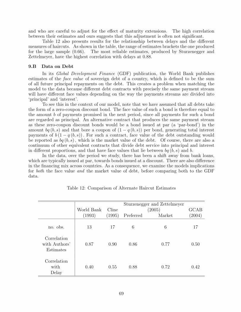
and who are careful to adjust for the effect of maturity extensions. The high correlationbetween their estimates and ours suggests that this adjustment is often not significant.

Table 12 also presents results for the relationship between delays and the differentmeasures of haircuts. As shown in the table, the range of estimates brackets the one producedfor the large sample (0.66). The most reliable estimates, produced by Sturzenegger andZettelmeyer, have the highest correlation with delays at 0.88.

9.B Data on Debt

In its Global Development Finance (GDF) publication, the World Bank publishesestimates of the face value of sovereign debt of a country, which is defined to be the sumof all future principal repayments on the debt. This creates a problem when matching themodel to the data because different debt contracts with precisely the same payment streamwill have different face values depending on the way the payments streams are divided into‘principal’ and ‘interest’.

To see this in the context of our model, note that we have assumed that all debts takethe form of a zero-coupon discount bond. The face value of such a bond is therefore equal tothe amount b of payments promised in the next period, since all payments for such a bondare regarded as principal. An alternative contract that produces the same payment streamas these zero-coupon discount bonds would be a bond issued at par (a ‘par-bond’) in theamount bq (b, s) and that bore a coupon of (1− q (b, s)) per bond, generating total interestpayments of b (1− q (b, s)) . For such a contract, face value of the debt outstanding wouldbe reported as bq (b, s) , which is the market value of the debt. Of course, there are also acontinuum of other equivalent contracts that divide debt service into principal and interestin different proportions, and that have face values that lie between bq (b, s) and b.

In the data, over the period we study, there has been a shift away from bank loans,which are typically issued at par, towards bonds issued at a discount. There are also differencein the financing mix across countries. As a consequence, we examine the models implicationsfor both the face value and the market value of debt, before comparing both to the GDFdata.

Table 12: Comparison of Alternate Haircut Estimates

Sturzenegger and ZettelmeyerWorld Bank Cline (2005) GCAB

(1993) (1995) Preferred Market (2004)

no. obs. 13 17 6 6 17

Correlationwith Authors’

Estimates0.87 0.90 0.86 0.77 0.50

CorrelationwithDelay

0.40 0.55 0.88 0.72 0.42

69

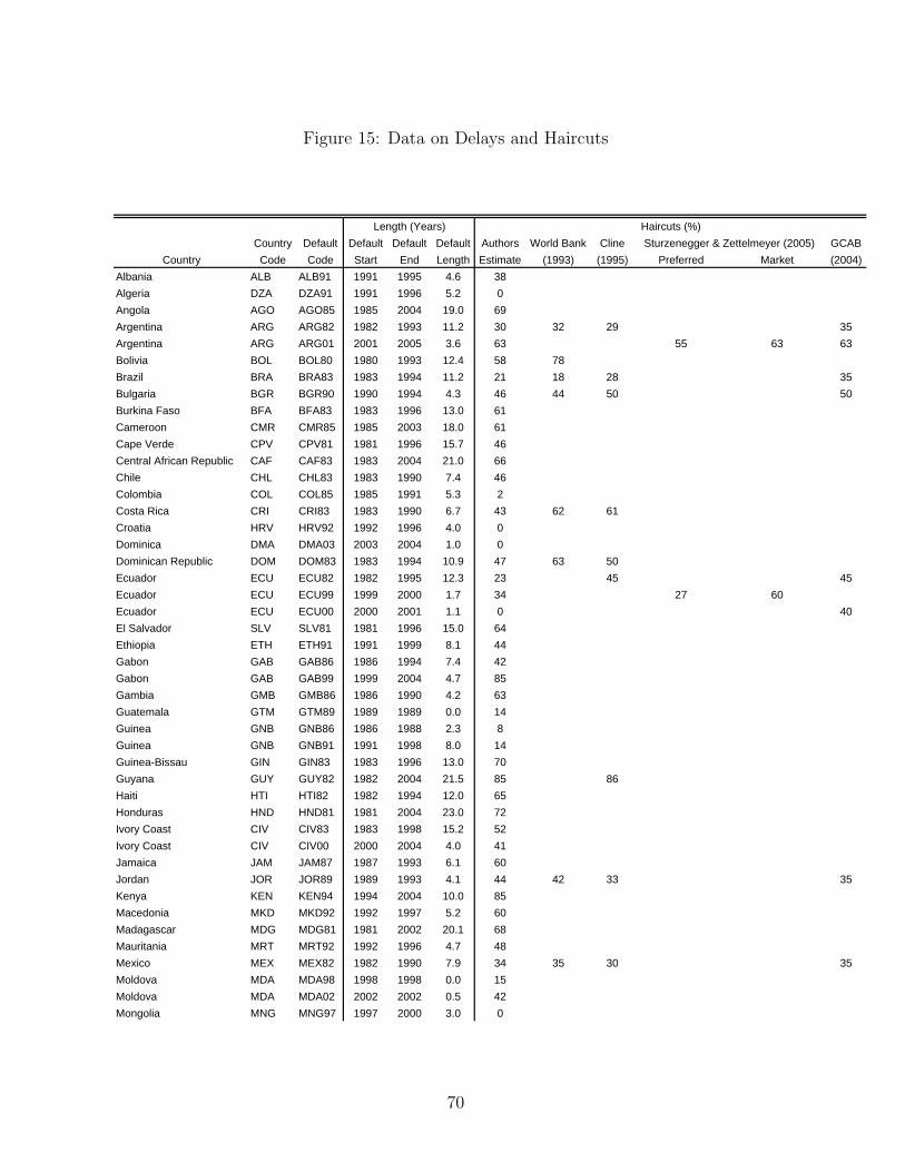
Figure 15: Data on Delays and Haircuts

Country Default Default Default Default Authors World Bank Cline GCABCountry Code Code Start End Length Estimate (1993) (1995) Preferred Market (2004)

Albania ALB ALB91 1991 1995 4.6 38Algeria DZA DZA91 1991 1996 5.2 0Angola AGO AGO85 1985 2004 19.0 69Argentina ARG ARG82 1982 1993 11.2 30 32 29 35Argentina ARG ARG01 2001 2005 3.6 63 55 63 63Bolivia BOL BOL80 1980 1993 12.4 58 78Brazil BRA BRA83 1983 1994 11.2 21 18 28 35Bulgaria BGR BGR90 1990 1994 4.3 46 44 50 50Burkina Faso BFA BFA83 1983 1996 13.0 61Cameroon CMR CMR85 1985 2003 18.0 61Cape Verde CPV CPV81 1981 1996 15.7 46Central African Republic CAF CAF83 1983 2004 21.0 66Chile CHL CHL83 1983 1990 7.4 46Colombia COL COL85 1985 1991 5.3 2Costa Rica CRI CRI83 1983 1990 6.7 43 62 61Croatia HRV HRV92 1992 1996 4.0 0Dominica DMA DMA03 2003 2004 1.0 0Dominican Republic DOM DOM83 1983 1994 10.9 47 63 50Ecuador ECU ECU82 1982 1995 12.3 23 45 45Ecuador ECU ECU99 1999 2000 1.7 34 27 60Ecuador ECU ECU00 2000 2001 1.1 0 40El Salvador SLV SLV81 1981 1996 15.0 64Ethiopia ETH ETH91 1991 1999 8.1 44Gabon GAB GAB86 1986 1994 7.4 42Gabon GAB GAB99 1999 2004 4.7 85Gambia GMB GMB86 1986 1990 4.2 63Guatemala GTM GTM89 1989 1989 0.0 14Guinea GNB GNB86 1986 1988 2.3 8Guinea GNB GNB91 1991 1998 8.0 14Guinea-Bissau GIN GIN83 1983 1996 13.0 70Guyana GUY GUY82 1982 2004 21.5 85 86Haiti HTI HTI82 1982 1994 12.0 65Honduras HND HND81 1981 2004 23.0 72Ivory Coast CIV CIV83 1983 1998 15.2 52Ivory Coast CIV CIV00 2000 2004 4.0 41Jamaica JAM JAM87 1987 1993 6.1 60Jordan JOR JOR89 1989 1993 4.1 44 42 33 35Kenya KEN KEN94 1994 2004 10.0 85Macedonia MKD MKD92 1992 1997 5.2 60Madagascar MDG MDG81 1981 2002 20.1 68Mauritania MRT MRT92 1992 1996 4.7 48Mexico MEX MEX82 1982 1990 7.9 34 35 30 35Moldova MDA MDA98 1998 1998 0.0 15Moldova MDA MDA02 2002 2002 0.5 42Mongolia MNG MNG97 1997 2000 3.0 0

Length (Years) Haircuts (%)Sturzenegger & Zettelmeyer (2005)

70

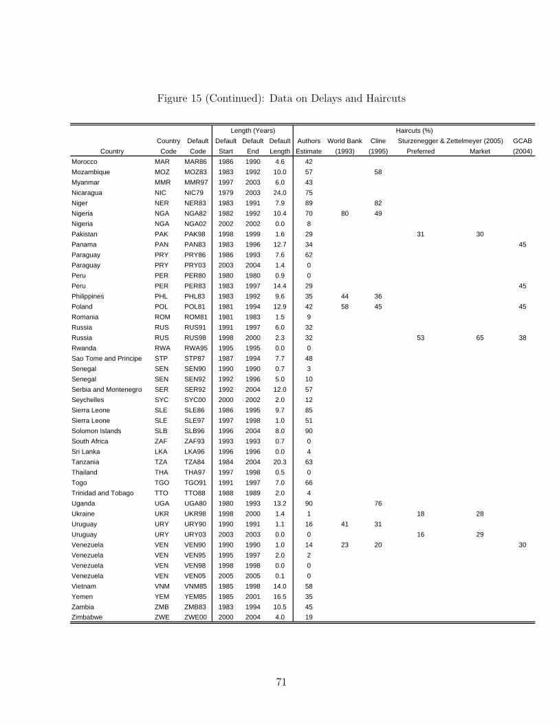
Figure 15 (Continued): Data on Delays and Haircuts

Country Default Default Default Default Authors World Bank Cline GCABCountry Code Code Start End Length Estimate (1993) (1995) Preferred Market (2004)

Length (Years) Haircuts (%)Sturzenegger & Zettelmeyer (2005)

Morocco MAR MAR86 1986 1990 4.6 42Mozambique MOZ MOZ83 1983 1992 10.0 57 58Myanmar MMR MMR97 1997 2003 6.0 43Nicaragua NIC NIC79 1979 2003 24.0 75Niger NER NER83 1983 1991 7.9 89 82Nigeria NGA NGA82 1982 1992 10.4 70 80 49Nigeria NGA NGA02 2002 2002 0.0 8Pakistan PAK PAK98 1998 1999 1.6 29 31 30Panama PAN PAN83 1983 1996 12.7 34 45Paraguay PRY PRY86 1986 1993 7.6 62Paraguay PRY PRY03 2003 2004 1.4 0Peru PER PER80 1980 1980 0.9 0Peru PER PER83 1983 1997 14.4 29 45Philippines PHL PHL83 1983 1992 9.6 35 44 36Poland POL POL81 1981 1994 12.9 42 58 45 45Romania ROM ROM81 1981 1983 1.5 9Russia RUS RUS91 1991 1997 6.0 32Russia RUS RUS98 1998 2000 2.3 32 53 65 38Rwanda RWA RWA95 1995 1995 0.0 0Sao Tome and Principe STP STP87 1987 1994 7.7 48Senegal SEN SEN90 1990 1990 0.7 3Senegal SEN SEN92 1992 1996 5.0 10Serbia and Montenegro SER SER92 1992 2004 12.0 57Seychelles SYC SYC00 2000 2002 2.0 12Sierra Leone SLE SLE86 1986 1995 9.7 85Sierra Leone SLE SLE97 1997 1998 1.0 51Solomon Islands SLB SLB96 1996 2004 8.0 90South Africa ZAF ZAF93 1993 1993 0.7 0Sri Lanka LKA LKA96 1996 1996 0.0 4Tanzania TZA TZA84 1984 2004 20.3 63Thailand THA THA97 1997 1998 0.5 0Togo TGO TGO91 1991 1997 7.0 66Trinidad and Tobago TTO TTO88 1988 1989 2.0 4Uganda UGA UGA80 1980 1993 13.2 90 76Ukraine UKR UKR98 1998 2000 1.4 1 18 28Uruguay URY URY90 1990 1991 1.1 16 41 31Uruguay URY URY03 2003 2003 0.0 0 16 29Venezuela VEN VEN90 1990 1990 1.0 14 23 20 30Venezuela VEN VEN95 1995 1997 2.0 2Venezuela VEN VEN98 1998 1998 0.0 0Venezuela VEN VEN05 2005 2005 0.1 0Vietnam VNM VNM85 1985 1998 14.0 58Yemen YEM YEM85 1985 2001 16.5 35Zambia ZMB ZMB83 1983 1994 10.5 45Zimbabwe ZWE ZWE00 2000 2004 4.0 19

71