
Recent Developments of the Theory of Tunneling 1 Faculty of Integmted Human Studies, Kyoto
56
INVITED PAPERS 1 Progress of Theoretical Physics, Vol. 127, No. 1, January 2012 Thermodynamics of Information Processing in Small Systems ˜) Takahiro Sagawa 1,2 1 The Hakubi Center, Kyoto University, Kyoto 606-8302, Japan 2 Yukawa Institute for Theoretical Physics, Kyoto University, Kyoto 606-8502, Japan (Received October 24, 2011) We review a general theory of thermodynamics of information processing. The back- ground of this topic is the recently-developed nonequilibrium statistical mechanics and quan- tum (and classical) information theory. These theories are closely related to the modern technologies to manipulate and observe small systems; for example, macromolecules and colloidal particles in the classical regime, and quantum-optical systems and quantum dots in the quantum regime. First, we review a generalization of the second law of thermodynamics to the situations in which small thermodynamic systems are subject to quantum feedback control. The gener- alized second law is expressed in terms of an inequality that includes the term of information obtained by the measurement, as well as the thermodynamic quantities such as the free energy. This inequality leads to the fundamental upper bound of the work that can be extracted by a “Maxwell’s demon”, which can be regarded as a feedback controller with a memory that stores measurement outcomes. Second, we review generalizations of the second law of thermodynamics to the measure- ment and information erasure processes of the memory of the demon that is a quantum system. The generalized second laws consist of inequalities that identify the lower bounds of the energy costs that are needed for the measurement and the information erasure. The inequality for the erasure leads to the celebrated Landauer’s principle for a special case. Moreover, these inequalities enable us to reconcile Maxwell’s demon with the second law of thermodynamics. In these inequalities, thermodynamic quantities and information contents are treated on an equal footing. In fact, the inequalities are model-independent, so that they can be applied to a broad class of information processing. Therefore, these inequalities can be called the second law of “information thermodynamics”. Subject Index: 058 §1. Introduction Information is physical. — Rolf Landauer It from bit. — John A. Wheeler In 1867, James C. Maxwell wrote a letter to Peter G. Tait. In the letter, Maxwell mentioned for the first time his gedankenexperiment of “a being whose faculties are so sharpened that he can follow every molecule”. 1) The being may be like a tiny fairy, and may violate the second law of thermodynamics. In 1874, William Thomson, who ∗) This review article is based on Chaps. 1 to 7 and Chap. 10 of the author’s Ph.D. thesis. Downloaded from https://academic.oup.com/ptp/article-abstract/127/1/1/1850101 by guest on 15 April 2019
Transcript of Recent Developments of the Theory of Tunneling 1 Faculty of Integmted Human Studies, Kyoto
INVITED PAPERS 1
Progress of Theoretical Physics, Vol. 127, No. 1, January 2012
Thermodynamics of Information Processing in Small Systems˜)
Takahiro Sagawa1,2
1The Hakubi Center, Kyoto University, Kyoto 606-8302, Japan2Yukawa Institute for Theoretical Physics, Kyoto University,
Kyoto 606-8502, Japan
(Received October 24, 2011)
We review a general theory of thermodynamics of information processing. The back-ground of this topic is the recently-developed nonequilibrium statistical mechanics and quan-tum (and classical) information theory. These theories are closely related to the moderntechnologies to manipulate and observe small systems; for example, macromolecules andcolloidal particles in the classical regime, and quantum-optical systems and quantum dotsin the quantum regime.
First, we review a generalization of the second law of thermodynamics to the situationsin which small thermodynamic systems are subject to quantum feedback control. The gener-alized second law is expressed in terms of an inequality that includes the term of informationobtained by the measurement, as well as the thermodynamic quantities such as the freeenergy. This inequality leads to the fundamental upper bound of the work that can beextracted by a “Maxwell’s demon”, which can be regarded as a feedback controller with amemory that stores measurement outcomes.
Second, we review generalizations of the second law of thermodynamics to the measure-ment and information erasure processes of the memory of the demon that is a quantumsystem. The generalized second laws consist of inequalities that identify the lower boundsof the energy costs that are needed for the measurement and the information erasure. Theinequality for the erasure leads to the celebrated Landauer’s principle for a special case.Moreover, these inequalities enable us to reconcile Maxwell’s demon with the second law ofthermodynamics.
In these inequalities, thermodynamic quantities and information contents are treated onan equal footing. In fact, the inequalities are model-independent, so that they can be appliedto a broad class of information processing. Therefore, these inequalities can be called thesecond law of “information thermodynamics”.
Subject Index: 058
§1. Introduction
Information is physical.— Rolf Landauer
It from bit.— John A. Wheeler
In 1867, James C. Maxwell wrote a letter to Peter G. Tait. In the letter, Maxwellmentioned for the first time his gedankenexperiment of “a being whose faculties areso sharpened that he can follow every molecule”.1) The being may be like a tiny fairy,and may violate the second law of thermodynamics. In 1874, William Thomson, who
∗) This review article is based on Chaps. 1 to 7 and Chap. 10 of the author’s Ph.D. thesis.
Dow
nloaded from https://academ
ic.oup.com/ptp/article-abstract/127/1/1/1850101 by guest on 15 April 2019

2 T. Sagawa
is also well-known as Lord Kelvin, gave it an impressive but opprobrious name —“demon”.
Ever since the birth of Maxwell’s demon, it has puzzled numerous physicistsover 150 years. The demon has shed light on the foundation of thermodynamics andstatistical mechanics, because it apparently contradicts the second law of thermo-dynamics.2)–8) Many researchers have tried to reconcile the demon with the secondlaw.9)
The first crucial step of the quantitative analysis of the demon was made byLeo Szilard in his paper published in 1929.10) He recognized the importance of theconcept of information to understand the paradox of Maxwell’s demon, about twentyyears before an epoch-making paper by Claude E. Shannon.11) As we will discuss indetail in the next section, Szilard considered that, if we take the role of informationinto account, the demon is shown to be consistent with the second law.
In 1951, Leon Brillouin considered that the key to resolve the paradox of Maxwell’sdemon is in the measurement process.12) On the other hand, Charles H. Bennett in-sisted that the measurement process is irrelevant to resolve the paradox of Maxwell’sdemon. Instead, in 1982, Bennett argued that the erasure process of the obtainedinformation is the key to reconcile the demon with the second law,13) based on Lan-dauer’s principle proposed by Rolf Landauer in 1961.14) The argument by Bennetthas been broadly accepted as the resolution of the paradox of Maxwell’s demon —until recently.9),15)
Let us next discuss the modern backgrounds of Maxwell’s demon. The recenttechnologies of controlling small systems have been developed in both classical andquantum regimes. For example, in the classical regime, one can manipulate a singlemacromolecule or a colloidal particle more precisely than the level of thermal fluctu-ations at room temperature, by using, for example, optical tweezers. This techniquehas been applied to investigate biological systems such as the molecular motors16)
(e.g., Kinesins and F1-ATPases). Moreover, artificial molecular machines17)–21) havealso been investigated in both terms of theories and experiments. In the quantumregime, both theories and experiments of quantum measurement and control havebeen developed at the level of a single atom or a single photon.
In particular with these developments, powerful theories have been establishedin nonequilibrium statistical mechanics and quantum information theory.
In nonequilibrium statistical mechanics, thermodynamic aspects of small sys-tems have become more and more important.22)–24) In the classical regime, macro-molecules and colloidal particles are typical examples of the small thermodynamicsystems. In the quantum regime, quantum dots can be regarded as a typical exam-ple. The crucial feature of such small thermodynamic systems is that their dynamicsis stochastic; their thermal or quantum fluctuations become the same order of mag-nitude as the averages of the physical quantities. Therefore, the fluctuations playcrucial roles to understand the dynamics of such systems. In this review article, wewill mainly focus on the thermal fluctuations in terms of nonequilibrium statisticalmechanics. Since 1993, a lot of equalities that are universally valid in nonequilib-rium stochastic systems have been found,25)–58) and they have been experimentally
Dow
nloaded from https://academ
ic.oup.com/ptp/article-abstract/127/1/1/1850101 by guest on 15 April 2019

Thermodynamics of Information Processing in Small Systems 3
verified.59)–69) A prominent result is the fluctuation theorem,25),26),28),29),33) whichenables us to quantitatively understand the probability of the stochastic violationof the second law of thermodynamics in small systems. Another prominent result isthe Jarzynski equality,27) which expresses the second law of thermodynamics by anequality rather than an inequality. From the first cumulant of the Jarzynski equality,we can reproduce the conventional second law of thermodynamics that is expressedin terms of an inequality. The second law of thermodynamics can be shown to stillhold on average even in small systems without Maxwell’s demon, while the secondlaw is stochastically violated in small systems due to the thermal fluctuations.
On the other hand, quantum measurement theory has been established, andhas been applied to a lot of systems including quantum-optical systems.70)–77) Theconcepts of positive operator-valued measures (POVMs) and measurement opera-tors play crucial roles, which enable us to quantitatively calculate the probabilitydistributions of the outcomes and the backactions of quantum measurements. Thesetheoretical concepts correspond to a lot of experimental situations in which one per-forms indirect measurements by using a measurement apparatus. Moreover, on thebasis of the quantum measurement theory, quantum information theory74) has alsobeen developed, which is a generalization of classical information theory proposedby Shannon.11),78)
On the basis of these backgrounds, Maxwell’s demon and thermodynamics of in-formation processing have been attracted renewed attentions.79)–116) In particular,Maxwell’s demon can be characterized as a feedback controller acting on thermody-namic systems.86),87) Here, “feedback” means that a control protocol depends onmeasurement outcomes obtained from the controlled system.117),118) Feedback con-trol is useful to experimentally realize intended dynamical properties of small systemsboth in classical and quantum systems. While feedback control has a long historymore than 50 years in science and engineering, the modern technologies enable usto control the thermal fluctuation at the level of kBT with kB being the Boltzmannconstant and T being the temperature. In fact, recently, Szilard-type Maxwell’s de-mon has been realized for the first time,116) by using a real-time feedback control ofa colloidal particle on a ratchet-type potential.
In this review article, we review a general theory of thermodynamics of informa-tion processing in small systems, by using both nonequilibrium statistical mechanicsand quantum information theory. The significances of this topic are:
• It sheds new light on the foundations of thermodynamics and statistical me-chanics.
• It is applicable to the analysis of the thermodynamic properties of a broad classof information processing.
In particular, we review generalizations of the second law of thermodynamics toinformation processing such as the feedback control, the measurement, and the in-formation erasure. The generalized second laws involve the terms of informationcontents, and identify the fundamental lower bounds of the energy costs that areneeded for the information processing in both classical and quantum regimes.
Dow
nloaded from https://academ
ic.oup.com/ptp/article-abstract/127/1/1/1850101 by guest on 15 April 2019
4 T. Sagawa
We also discuss an explicit counter-example against Bennett’s argument to re-solve the paradox of Maxwell’s demon, and discuss a general and quantitative wayto reconcile the demon with the second law. The paradox of Maxwell’s demon hasbeen essentially resolved by this argument.
This review article is based on Chaps. 1 to 7 and Chap. 10 of the author’s Ph.D.thesis. The organization of this article is as follows.
In §2, we review the basic concepts and the history of the problem of Maxwell’sdemon. Starting from the review of the original gedankenexperiment by Maxwell,we discuss the arguments by Szilard, Brillouin, Landauer, and Bennett.
To generally formulate Maxwell’s demon in a model-independent way, we needmodern information theory which will be reviewed in §§3 and 4. In §3, we focuson the classical aspects: we review the general formulations of classical stochasticdynamics, information, and measurement. The key concepts in this section are theShannon information and the mutual information. In §4, we focus on the quantumaspects of information theory. Starting from the formulation of the dynamics ofunitary and nonunitary quantum systems, we shortly review quantum measurementtheory and quantum information theory. In particular, we discuss the concept ofQC-mutual information and prove its important properties. Moreover, we discussthat the quantum formulation includes the classical one as a special case, by pointingout the quantum-classical correspondence. Therefore, while we discuss only quantumformulations in §§5, 6, and 7, the formulations and results include classical ones.
In §5, we review the possible derivations of the second law of thermodynamics.In particular, we discuss the proof of the second law in terms of the unitary evolutionof the total system including multi-heat baths with the initial canonical distributions.This approach to prove the second law is the standard one in modern nonequilibriumstatistical mechanics. We derive several inequalities including Kelvin’s inequality, theClausius inequality, and its generalization to nonequilibrium initial and final states.The proof is independent of the size of the thermodynamic system, and can beapplied to small thermodynamic systems.
Section 6 is the first main part of this article. We review a generalized secondlaw of thermodynamics with a single quantum measurement and quantum feedbackcontrol, by involving the measurement and feedback to the proof in §5 in line withRef. 87). The QC-mutual information discussed in §4 characterizes the upper boundof the additional work that can be extracted from heat engines with the assistanceof feedback control, or Maxwell’s demon.
In §7, we review the thermodynamic aspects of Maxwell’s demon itself (or thememory of the feedback controller), which is the second main part of this article.Starting from the formulation of the memory that stores measurement outcomes, weidentify the lower bounds of the thermodynamic energy costs for the measurementand the information erasure, which are the main results of Ref. 97). These resultscan be regarded as the generalizations of the second law of thermodynamics to themeasurement and the information erasure processes. In particular, the result for theerasure includes Landauer’s principle as a special case.
By using the general arguments in §§6 and 7, we can essentially reconcile Maxwell’s
Dow
nloaded from https://academ
ic.oup.com/ptp/article-abstract/127/1/1/1850101 by guest on 15 April 2019

Thermodynamics of Information Processing in Small Systems 5
demon with the second law of thermodynamics. This is a novel and general phys-ical picture of the resolution of the paradox of Maxwell’s demon, which has beendiscussed in Ref. 97).
In §8, we conclude this article.
§2. Review of Maxwell’s demon
In this section, we review the basic ideas related to the problem of Maxwell’sdemon.
2.1. Original Maxwell’s Demon
First of all, we consider the original version of the demon proposed by Maxwell(see also Fig. 1).1) A classical ideal gas is in a box that is adiabatically separated fromthe environment. In the initial state, the gas is in thermal equilibrium at temperatureT . Suppose that a barrier is inserted at the center of the box, and a small door isattached to the barrier. A small being, which is named as a “demon” by Kelvin,is in the front of the door. It has the capability of measuring the velocity of eachmolecule in the gas, and it opens or closes the door depending on the measurementoutcomes. If a molecule whose velocity is higher than the averaged one comes fromthe left box, then the demon opens the door. If a molecule whose velocity is slowerthan the average one comes from the right box, then the demon also opens thedoor. Otherwise the door is closed. By repeating this operation again and again,the gas in the left box gradually becomes cooler than the initial temperature, andthe gas in the right box becomes hotter. After all, the demon is able to adiabaticallycreate the temperature difference starting from the initial uniform temperature. Inother words, the entropy of the gas is more and more decreased by the action of thedemon, though the box is adiabatically separated from the outside. This apparentcontradiction to the second law has been known as the paradox of Maxwell’s demon.
The important point of this gedankenexperiment is that the demon can performthe measurement at the single-molecule level, and can control the door based onthe measurement outcomes (i.e., the molecule’s velocity is faster or slower than theaverage), which implies the demon can perform feedback control of the thermalfluctuation.
Fig. 1. The original gedankenexperiment of Maxwell’s demon. A white (black) particle indicates a
molecule whose velocity is slower (faster) than the average. The demon adiabatically realizes a
temperature difference by measuring the velocities of molecules and controlling the door based
on the measurement outcomes.
Dow
nloaded from https://academ
ic.oup.com/ptp/article-abstract/127/1/1/1850101 by guest on 15 April 2019

6 T. Sagawa
2.2. Szilard Engine
The first crucial model of Maxwell’s demon that quantitatively clarified therole of the information was proposed by Szilard in 1929.10) The setup by Szilardseems to be a little different from Maxwell’s one, but the essence — the role of themeasurement and feedback — is the same.
Let us consider a classical single molecule gas in an isothermal box that contactswith a single heat bath at temperature T . Szilard’s engine consists of the followingfive steps (see also Fig. 2).
Step 1: Initial state. In the initial state, a single molecule is in thermal equilib-rium at temperature T .
Step 2: Insertion of the barrier. We next insert a barrier at the center of thebox, so that we divide the box into two boxes. In this stage, we do not know whichbox the molecule is in. In the ideal case, we do not need any work for this insertionprocess.
Step 3: Measurement. The demon then measures the position of the molecule,and finds whether the molecule is in “left” or “right”. This measurement is assumedto be error-free. The information obtained by the demon is 1 bit, which equalsln 2 nat in the natural logarithm, corresponding to the binary outcome of “left” or“right”. The rigorous formulation of the concept of information will be discussed inthe next section.
Step 4: Feedback. The demon next performs the control depending on the mea-
Fig. 2. Schematic of the Szilard engine. Step 1: Initial equilibrium state of a single molecule at
temperature T . Step 2: Insertion of the barrier. Step 3: Measurement of the position of the
molecule. The demon gets I = ln 2 nat of information. Step 4: Feedback control. The demon
moves the box to the left only if the measurement outcome is “right”. Step 5: Work extraction
by the isothermal and quasi-static expansion. The state of the engine then returns to the initial
one. During this isothermal cycle, we can extract kBT ln 2 of work.
Dow
nloaded from https://academ
ic.oup.com/ptp/article-abstract/127/1/1/1850101 by guest on 15 April 2019

Thermodynamics of Information Processing in Small Systems 7
surement outcome, which is regarded as a feedback control. If the outcome is “left”,then the demon does nothing. On the other hand, if the outcome is “right”, then thedemon quasi-statically moves the right box to the left position. No work is neededfor this process, because the motion of the box is quasi-static. After this feedbackprocess, the state of the system is independent of the measurement outcome; thepost-feedback state is always “left”.
Step 5: Extraction of the work. We then expand the left box quasi-statically andisothermally, so that the system returns to the initial state. Since the expansion isquasi-static and isothermal, the equation of states of the single-molecular ideal gasalways holds:
pV = kBT, (2.1)
where p is the pressure, V is the volume, and kB is the Boltzmann constant. There-fore, we extract Wext = kBT ln 2 of work during this expansion, which is followedfrom
Wext =∫ V0
V0/2dV
kBT
V= kBT ln 2, (2.2)
where V0 is the initial volume of the box.
During the total process described above, we can extract the positive work ofkBT ln 2 from the isothermal cycle with the assistance of the demon. This apparentlycontradicts the second law of thermodynamics for isothermal processes known asKelvin’s principle, which states that we cannot extract any positive work from anyisothermal cycle in the presence of a single heat bath. In fact, if one could violateKelvin’s principle, one was able to create a perpetual motion of the second kind.Therefore, the fundamental problem is the following:
• Is the Szilard engine a perpetual motion of the second kind?• If not, what compensates for the excess work of kBT ln 2?
This is the problem of Maxwell’s demon.The crucial feature of the Szilard engine lies in the fact that the extracted work of
kBT ln 2 is proportional to the obtained information ln 2 with the coefficient of kBT .Therefore, it would be expected that the information plays a key role to resolve theparadox of Maxwell’s demon. In fact, from Step 2 to Step 4, the demon decreaseskB ln 2 of physical entropy corresponding to the thermal fluctuation between “left”or “right”, by using ln 2 of information. Immediately after the measurement in Step3, the state of the molecule and the measurement outcome are perfectly correlated,which implies that the demon has the perfect information about the measured state(i.e., “left” or “right”). However, immediately after the feedback in Step 5, the stateof the molecule and the measurement outcome is no longer correlated. Therefore,we can conclude that the demon uses the obtained information as a resource todecrease the physical entropy of the system. This is the bare essential of the Szilardengine. On the other hand, the decrease of kB ln 2 of the entropy means the increaseof kBT ln 2 of the Helmholtz free energy, because F = E − TS holds with F beingthe free energy, E being the internal energy, and S being the entropy. Therefore,
Dow
nloaded from https://academ
ic.oup.com/ptp/article-abstract/127/1/1/1850101 by guest on 15 April 2019
8 T. Sagawa
the free energy is increased by kBT ln 2 during the feedback control by the demon,and the increase in the free energy has been extracted as the work in Step 5. Thisis how the information has been used in the Szilard engine to extract the positivework.
Szilard pointed out that the increase of the entropy in the memory of the demoncompensates for the decrease of the entropy of kB ln 2 by feedback control. In fact,the memory of the demon, which stores the obtained information of “left” or “right”,is itself a physical system, and the fluctuation of the measurement outcome impliesan increase in the physical entropy of the memory. In fact, to decrease kB ln 2 of thephysical entropy of the controlled system (i.e., the Szilard engine), at least the sameamount of physical entropy must increase elsewhere corresponding to the obtainedinformation, so that the second law of thermodynamics for the total system of theSzilard engine and demon’s memory is not violated. This is a crucial observationmade by Szilard. However, it was not yet so clear which process actually compensatesfor the excess work of kBT ln 2. This problem has been investigated by Brillouin,Landauer, and Bennett.
2.3. Brillouin’s Argument
In 1951, Brillouin made an important argument on the problem of Maxwell’sdemon.12) He considered that the excess work of kBT ln 2 is compensated for by thework that is needed for the measurement process by the demon.
He considered that the demon needs to shed a probe light, which is at least asingle photon, to the molecule to detect its position. However, if the temperatureof the heat bath is T , there must be the background radiation around the molecule.The energy of a photon of the background radiation is about kBT . Therefore, todistinguish the probe photon from the background photons, the energy of the probephoton should be much greater than that of the background photons:
�ωP � kBT, (2.3)
where ωP is the frequency of the probe photon. Inequality (2.3) may imply
Wmeas = �ωP > kBT ln 2, (2.4)
which means that the energy cost Wmeas that is needed for the measurement shouldbe larger than the excess work of kBT ln 2. Therefore, Brillouin considered that theenergy cost for the measurement process compensates for the excess work, so thatwe cannot extract any positive work from the Szilard engine.
We note that, from the modern point of view, Brillouin’s argument depends ona specific model to measure the position of the molecule.
2.4. Landauer’s Principle
On the other hand, in his paper published in 1961,14) Landauer considered thefundamental energy cost that is needed for the erasure of the obtained informa-tion from the memory. He propose an important observation, which is known asLandauer’s principle today: to erase one bit (= ln 2 nat) of information from the
Dow
nloaded from https://academ
ic.oup.com/ptp/article-abstract/127/1/1/1850101 by guest on 15 April 2019

Thermodynamics of Information Processing in Small Systems 9
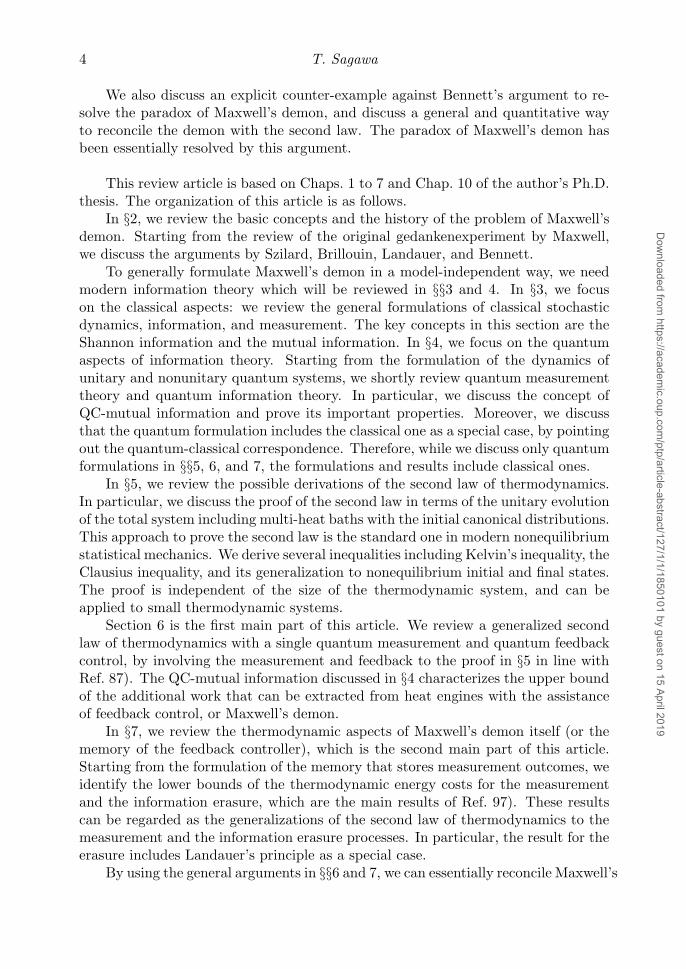
Fig. 3. Schematic of information erasure. Before the erasure, the memory stores information “0”
or “1”. After the erasure, the memory goes back to the standard state “0” with unit probability.
memory in the presence of a single heat bath at temperature T , at least kBT ln 2 ofheat should be dissipated from the memory to the environment.
This statement can be understood as follows. Before the information erasure,the memory stores ln 2 of information, which can be represented by “0” and “1”.For example, as shown in Fig. 3, if the particle is in the left well, the memory storesthe information of “0”, while if the particle is in the right well, the memory storesinformation of “1”. This information storage corresponds to kB ln 2 of entropy ofthe memory. After the information erasure, the state of the memory is reset to thestandard state, say “0” with unit probability as shown in Fig. 3. The entropy ofthe memory then decreases by kB ln 2 during the information erasure. According tothe conventional second law of thermodynamics, the decrease of the entropy in anyisothermal process should be accompanied by the heat dissipation to the environ-ment. Therefore, during the erasure process, at least kBT ln 2 of heat is dissipatedfrom the memory to the heat bath, corresponding to the decrease of the entropy ofkB ln 2. This is the physical origin of Landauer’s principle, which is closely relatedto the second law of thermodynamics.
If the internal energies of “0” and “1” are degenerate, we need the same amountof the work as the heat to compensate for the heat dissipation. Therefore, Landauer’sprinciple can be also stated as
Weras ≥ kBT ln 2, (2.5)
where Weras is the work that is needed for the erasure process.The argument by Landauer seems to be very general and model-independent,
because it is a consequence of the second law of thermodynamics. However, theproof of Landauer’s principle based on statistical mechanics has been given only fora special type of memories that is represented by the symmetric binary potentialdescribed in Fig. 3.89),92) We note that Goto and his collaborators argued that thereis a counter-example of Landauer’s principle.91)
Dow
nloaded from https://academ
ic.oup.com/ptp/article-abstract/127/1/1/1850101 by guest on 15 April 2019
10 T. Sagawa
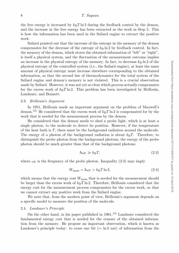
Fig. 4. Logical reversibility and irreversibility. (a) Logically reversible measurement process.
(b) Logically irreversible erasure process.
2.5. Bennett’s Argument
In 1982, Bennett proposed an explicit example in which we do not need any en-ergy cost to perform a measurement, which implies that there is a counter-exampleagainst Brillouin’s argument.13) Moreover, Bennett argued that, based on Lan-dauer’s principle (2.5), we always need the energy cost for information erasure fromdemon’s memory, which compensates for the excess work of kBT ln 2 that is extractedfrom the Szilard engine by the demon.
His proposal of the resolution of the paradox of Maxwell’s demon can be sum-marized as follows. To make the total system of the Szilard engine and demon’smemory a thermodynamic cycle, we need to reset the memory’s state which corre-sponds to information erasure. While we do not necessarily need for the work for themeasurement, at least kBT ln 2 of work is always needed the work for the erasure.Therefore, the information erasure is the key to reconcile the demon with the secondlaw of thermodynamics.
Bennett’s argument is also related to the concept of logical reversibility of clas-sical information processing. For example, the classical measurement process islogically reversible, while the erasure process is logically irreversible in classical in-formation theory. To see this, let us consider a classical binary measured system Sand a binary memory M. As shown in Fig. 4 (a), before the measurement, the stateof M is in the standard state “0” with unit probability, while the state of S is in“0” or “1”. After the measurement, the state of M changes according to the stateof S, and the states of M and S are perfectly correlated. In terminology of theoryof computation, this process corresponds to the C-NOT gate, where M is the targetbit. We stress that there is a one-to-one correspondence of the pre-measurement andthe post-measurement states of the total system of M and S, which implies that themeasurement process is logically reversible.
On the other hand, in the erasure process, measured system S is detached frommemory M, and the state of M returns to the standard state “0” with unit proba-bility, irrespective of the pre-erasure state. Figure 4 (b) shows this process. Clearly,there is no one-to-one correspondence between the pre-erasure and the post-erasurestates. In other words, the erasure process is not bijective. Therefore, the informa-
Dow
nloaded from https://academ
ic.oup.com/ptp/article-abstract/127/1/1/1850101 by guest on 15 April 2019
Thermodynamics of Information Processing in Small Systems 11
tion erasure is logically irreversible.In the logically reversible process, we may conclude that the entropy of the
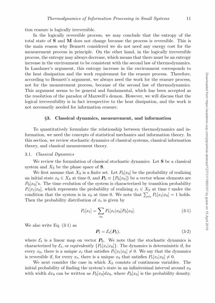
total state of S and M does not change because the process is reversible. This isthe main reason why Bennett considered we do not need any energy cost for themeasurement process in principle. On the other hand, in the logically irreversibleprocess, the entropy may always decrease, which means that there must be an entropyincrease in the environment to be consistent with the second law of thermodynamics.In Landauer’s argument, this entropy increase in the environment corresponds tothe heat dissipation and the work requirement for the erasure process. Therefore,according to Bennett’s argument, we always need the work for the erasure process,not for the measurement process, because of the second law of thermodynamics.This argument seems to be general and fundamental, which has been accepted asthe resolution of the paradox of Maxwell’s demon. However, we will discuss that thelogical irreversibility is in fact irrespective to the heat dissipation, and the work isnot necessarily needed for information erasure.
§3. Classical dynamics, measurement, and information
To quantitatively formulate the relationship between thermodynamics and in-formation, we need the concepts of statistical mechanics and information theory. Inthis section, we review stochastic dynamics of classical systems, classical informationtheory, and classical measurement theory.
3.1. Classical Dynamics
We review the formulation of classical stochastic dynamics. Let S be a classicalsystem and XS be the phase space of S.
We first assume that XS is a finite set. Let P0[x0] be the probability of realizingan initial state x0 ∈ XS at time 0, and P0 ≡ {P0[x0]} be a vector whose elements areP0[x0]’s. The time evolution of the system is characterized by transition probabilityPt[xt|x0], which represents the probability of realizing xt ∈ XS at time t under thecondition that the system is in x0 at time 0. We note that
∑xtPt[xt|x0] = 1 holds.
Then the probability distribution of xt is given by
Pt[xt] =∑x0
Pt[xt|x0]P0[x0]. (3.1)
We also write Eq. (3.1) asPt = Et(P0), (3.2)
where Et is a linear map on vector P0. We note that the stochastic dynamics ischaracterized by Et, or equivalently {Pt[xt|x0]}. The dynamics is deterministic if, forevery x0, there is a unique xt that satisfies Pt[xt|x0] �= 0. We say that the dynamicsis reversible if, for every xt, there is a unique x0 that satisfies Pt[xt|x0] �= 0.
We next consider the case in which XS consists of continuous variables. Theinitial probability of finding the system’s state in an infinitesimal interval around x0
with width dx0 can be written as P0[x0]dx0, where P0[x0] is the probability density.
Dow
nloaded from https://academ
ic.oup.com/ptp/article-abstract/127/1/1/1850101 by guest on 15 April 2019
12 T. Sagawa
We also write the probability density of xt as Pt[xt]. Let Pt[xt|x0] be the probabilitydensity of realizing xt ∈ XS at time t under the condition that the system is in x0
at time 0. Then we have
Pt[xt] =∫dx0Pt[xt|x0]P0[x0] (3.3)
for the case of continuous variables.
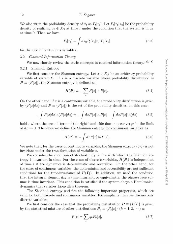
3.2. Classical Information Theory
We now shortly review the basic concepts in classical information theory.11),78)
3.2.1. Shannon EntropyWe first consider the Shannon entropy. Let x ∈ XS be an arbitrary probability
variable of system S. If x is a discrete variable whose probability distribution isP ≡ {P [x]}, the Shannon entropy is defined as
H(P ) ≡ −∑
x
P [x] lnP [x]. (3.4)
On the other hand, if x is a continuous variable, the probability distribution is givenby {P [x]dx} and P ≡ {P [x]} is the set of the probability densities. In this case,
−∫P [x]dx ln(P [x]dx) = −
∫dxP [x] lnP [x] −
∫dxP [x] ln(dx) (3.5)
holds, where the second term of the right-hand side does not converge in the limitof dx→ 0. Therefore we define the Shannon entropy for continuous variables as
H(P ) ≡ −∫dxP [x] lnP [x]. (3.6)
We note that, for the cases of continuous variables, the Shannon entropy (3.6) is notinvariant under the transformation of variable x.
We consider the condition of stochastic dynamics with which the Shannon en-tropy is invariant in time. For the cases of discrete variables, H(Pt) is independentof time t if the dynamics is deterministic and reversible. On the other hand, forthe cases of continuous variables, the determinism and reversibility are not sufficientconditions for the time-invariance of H(Pt). In addition, we need the conditionthat the integral element dxt is time-invariant, or equivalently, the phase-space vol-ume is time-invariant. This condition is satisfied if the system obeys a Hamiltoniandynamics that satisfies Liouville’s theorem.
The Shannon entropy satisfies the following important properties, which arevalid for both discrete and continuous variables. For simplicity, here we discuss onlydiscrete variables.
We first consider the case that the probability distribution P ≡ {P [x]} is givenby the statistical mixture of other distributions Pk ≡ {Pk[x]} (k = 1, 2, · · · ) as
P [x] =∑
k
qkPk[x], (3.7)
Dow
nloaded from https://academ
ic.oup.com/ptp/article-abstract/127/1/1/1850101 by guest on 15 April 2019
Thermodynamics of Information Processing in Small Systems 13
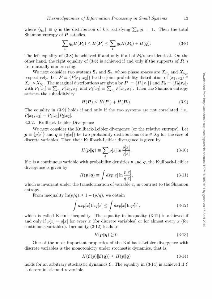
where {qk} ≡ q is the distribution of k’s, satisfying∑
k qk = 1. Then the totalShannon entropy of P satisfies∑
k
qkH(Pk) ≤ H(P ) ≤∑
k
qkH(Pk) +H(q). (3.8)
The left equality of (3.8) is achieved if and only if all of Pk’s are identical. On theother hand, the right equality of (3.8) is achieved if and only if the supports of Pk’sare mutually non-crossing.
We next consider two systems S1 and S2, whose phase spaces are XS1 and XS2 ,respectively. Let P ≡ {P [x1, x2]} be the joint probability distribution of (x1, x2) ∈XS1×XS2 . The marginal distributions are given by P1 ≡ {P1[x1]} and P2 ≡ {P2[x2]}with P1[x1] ≡
∑x2P [x1, x2] and P2[x2] ≡
∑x1P [x1, x2]. Then the Shannon entropy
satisfies the subadditivity
H(P ) ≤ H(P1) +H(P2). (3.9)
The equality in (3.9) holds if and only if the two systems are not correlated, i.e.,P [x1, x2] = P1[x1]P2[x2].
3.2.2. Kullback-Leibler DivergenceWe next consider the Kullback-Leibler divergence (or the relative entropy). Let
p ≡ {p[x]} and q ≡ {q[x]} be two probability distributions of x ∈ XS for the case ofdiscrete variables. Then their Kullback-Leibler divergence is given by
H(p‖q) ≡∑
x
p[x] lnp[x]q[x]
. (3.10)
If x is a continuous variable with probability densities p and q, the Kullback-Leiblerdivergence is given by
H(p‖q) ≡∫dxp[x] ln
p[x]q[x]
, (3.11)
which is invariant under the transformation of variable x, in contrast to the Shannonentropy.
From inequality ln(p/q) ≥ 1 − (p/q), we obtain∫dxp[x] ln q[x] ≤
∫dxp[x] ln p[x], (3.12)
which is called Klein’s inequality. The equality in inequality (3.12) is achieved ifand only if p[x] = q[x] for every x (for discrete variables) or for almost every x (forcontinuous variables). Inequality (3.12) leads to
H(p‖q) ≥ 0. (3.13)
One of the most important properties of the Kullback-Leibler divergence withdiscrete variables is the monotonicity under stochastic dynamics, that is,
H(E(p)‖E(q)) ≤ H(p‖q) (3.14)
holds for an arbitrary stochastic dynamics E . The equality in (3.14) is achieved if Eis deterministic and reversible.
Dow
nloaded from https://academ
ic.oup.com/ptp/article-abstract/127/1/1/1850101 by guest on 15 April 2019

14 T. Sagawa
3.2.3. Mutual InformationWe next consider the mutual information between two systems S1 and S2. Let
XS1 and XS2 be phase spaces of S1 and S2, respectively. Let P ≡ {P [x1, x2]} be thejoint probability distribution of (x1, x2) ∈ XS1 × XS2 . The marginal distributionsare given by P1 ≡ {P1[x1]} and P2 ≡ {P2[x2]} with P1[x1] ≡ ∑
x2P [x1, x2] and
P2[x2] ≡∑
x1P [x1, x2]. Then the mutual information is given by
I(S1 : S2) ≡ H(P1) +H(P2) −H(P ), (3.15)
which represents the correlation between the two systems. Mutual information (3.15)can be rewritten as
I(S1 : S2) =∑x1,x2
P [x1, x2] lnP [x1, x2]
P1[x1]P2[x2]= H(P ‖P ′), (3.16)
where P ′ ≡ {P1[x1]P2[x2]}. From Eq. (3.16) and inequality (3.9), we find that themutual information satisfies
I(S1 : S2) ≥ 0, (3.17)
where I(S1 : S2) = 0 is achieved if and only if P [x1, x2] = P1[x1]P2[x2] holds, orequivalently, if the two systems are not correlated. We can also show that
0 ≤ I(S1 : S2) ≤ H(P1), 0 ≤ I(S1 : S2) ≤ H(P2). (3.18)
Here, I(S1 : S2) = H(P1) holds if x1 is determined only by x2, and I(S1 : S2) =H(P2) holds if x2 is determined only by x1.
We note that, for the case of continuous variables, Eq. (3.16) can be written as
I(S1 : S2) =∫dx1dx2P [x1, x2] ln
P [x1, x2]P1[x1]P2[x2]
= H(P ‖P ′), (3.19)
which is invariant under the transformation of variables x1 and x2.
3.3. Classical Measurement Theory
We next review the general theory of a measurement on a classical system.Although the following argument can be applied to both continuous and discretevariables, for simplicity, we mainly concern the continuous variable cases.
Let x ∈ XS be an arbitrary probability variable of measured system S, andP ≡ {P [x]} be the probability distribution or the probability densities of x. Weperform a measurement on S and obtain outcome y. We note that y is also aprobability variable. If the measurement is error-free, x = y holds, in other words,x and y are perfectly correlated. In general, stochastic errors are involved in themeasurement, so that the correlation between x and y is not perfect. The errors canbe characterized by conditional probability P [y|x], which represents the probabilityof obtaining outcome y under the condition that the true value of the measuredsystem is x. We note that
∫dyP [y|x] = 1 for all x, where the integral is replaced by
the summation if x is a discrete variable. In the case of an error-free measurement,P [y|x] is given by the delta function (or Kronecker’s delta) such that x = y holds.
Dow
nloaded from https://academ
ic.oup.com/ptp/article-abstract/127/1/1/1850101 by guest on 15 April 2019
Thermodynamics of Information Processing in Small Systems 15
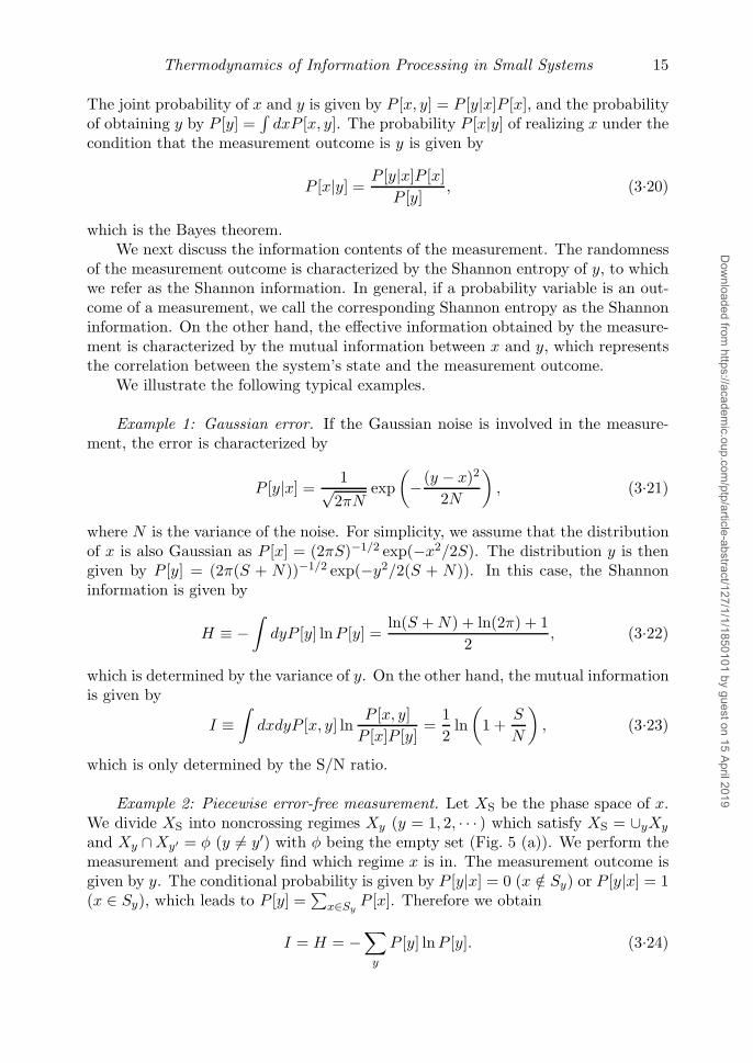
The joint probability of x and y is given by P [x, y] = P [y|x]P [x], and the probabilityof obtaining y by P [y] =
∫dxP [x, y]. The probability P [x|y] of realizing x under the
condition that the measurement outcome is y is given by
P [x|y] =P [y|x]P [x]
P [y], (3.20)
which is the Bayes theorem.We next discuss the information contents of the measurement. The randomness
of the measurement outcome is characterized by the Shannon entropy of y, to whichwe refer as the Shannon information. In general, if a probability variable is an out-come of a measurement, we call the corresponding Shannon entropy as the Shannoninformation. On the other hand, the effective information obtained by the measure-ment is characterized by the mutual information between x and y, which representsthe correlation between the system’s state and the measurement outcome.
We illustrate the following typical examples.
Example 1: Gaussian error. If the Gaussian noise is involved in the measure-ment, the error is characterized by
P [y|x] =1√
2πNexp
(−(y − x)2
2N
), (3.21)
where N is the variance of the noise. For simplicity, we assume that the distributionof x is also Gaussian as P [x] = (2πS)−1/2 exp(−x2/2S). The distribution y is thengiven by P [y] = (2π(S + N))−1/2 exp(−y2/2(S + N)). In this case, the Shannoninformation is given by
H ≡ −∫dyP [y] lnP [y] =
ln(S +N) + ln(2π) + 12
, (3.22)
which is determined by the variance of y. On the other hand, the mutual informationis given by
I ≡∫dxdyP [x, y] ln
P [x, y]P [x]P [y]
=12
ln(
1 +S
N
), (3.23)
which is only determined by the S/N ratio.
Example 2: Piecewise error-free measurement. Let XS be the phase space of x.We divide XS into noncrossing regimes Xy (y = 1, 2, · · · ) which satisfy XS = ∪yXy
and Xy ∩Xy′ = φ (y �= y′) with φ being the empty set (Fig. 5 (a)). We perform themeasurement and precisely find which regime x is in. The measurement outcome isgiven by y. The conditional probability is given by P [y|x] = 0 (x /∈ Sy) or P [y|x] = 1(x ∈ Sy), which leads to P [y] =
∑x∈Sy
P [x]. Therefore we obtain
I = H = −∑
y
P [y] lnP [y]. (3.24)
Dow
nloaded from https://academ
ic.oup.com/ptp/article-abstract/127/1/1/1850101 by guest on 15 April 2019

16 T. Sagawa
Fig. 5. (a) Piecewise error-free measurement. The total phase space is divided into subspaces
S1, S2, · · · . We measure which subspace the system is in. (b) Binary-symmetric channel with
error rate ε.
We note that H ≤ Hx holds, where Hx ≡ −∑x P [x] lnP [x] is the Shannon infor-mation of the measured system.
Example 3: Binary symmetric channel. We assume that both x and y take 0 or1. The conditional probabilities are given by
P [0|0] = P [1|1] = 1 − ε, P [0|1] = P [1|0] = ε, (3.25)
where ε is the error rate satisfying 0 ≤ ε ≤ 1 (Fig. 5 (b)). For an arbitrary probabilitydistribution of x, the Shannon information and the mutual information are relatedas
I = H −H(ε), (3.26)
where H(ε) ≡ −ε ln ε − (1 − ε) ln(1 − ε). We note that I = H holds if and only ifε = 0 or 1, and that I = 0 holds if and only if ε = 1/2.
§4. Quantum dynamics, measurement, and information
We next review the theory of quantum dynamics, measurement, and informa-tion.74) The classical measurement theory is shown to be a special case of thequantum measurement theory. In the followings, we will focus on quantum systemsthat correspond to finite-dimensional Hilbert spaces for simplicity. In the followings,we set � = 1.
4.1. Quantum Dynamics
First of all, we discuss the theory of quantum dynamics without any measure-ment. We first discuss the unitary dynamics, and next the nonunitary dynamics inopen systems.
4.1.1. Unitary EvolutionsWe consider a quantum system S corresponding to a finite-dimensional Hilbert
space H. Let |ψ〉 ∈ H be a pure state with 〈ψ|ψ〉 = 1. If system S is isolated fromany other quantum systems, the time evolution of state vector |ψ〉 is described bythe Schrodinger equation
id
dt|ψ(t)〉 = H(t)|ψ(t)〉, (4.1)
Dow
nloaded from https://academ
ic.oup.com/ptp/article-abstract/127/1/1/1850101 by guest on 15 April 2019
Thermodynamics of Information Processing in Small Systems 17
where H(t) is the Hamiltonian of this system. The formal solution of Eq. (4.1) isgiven by
|ψ(t)〉 = U(t)|ψ(0)〉, (4.2)
where U(t) is the unitary operator that is given by
U(t) ≡ T exp(−i∫H(t)dt
), (4.3)
where T denotes the time-ordered product.A statistical mixture of pure states is called a mixed state. It is described by a
Hermitian operator ρ acting on H, which we call a density operator. The statisticalmixture of pure states {|ξj〉} with probability distribution {qj} satisfying
∑j qj = 1
with qj ≥ 0 corresponds to density operator
ρ =∑
i
qi|ξi〉〈ξi|. (4.4)
In the case of pure state |ψ〉, the corresponding density operator is given by ρ =|ψ〉〈ψ|. From Eq. (4.4), it can easily be shown that
ρ ≥ 0 (4.5)
andtr(ρ) = 1. (4.6)
Conversely, any Hermitian operator satisfying (4.5) and (4.6) can be decomposed as
ρ =∑
i
qi|φi〉〈φi|, (4.7)
where {qi} is a probability distribution satisfying∑
i qi = 1, and {|φi〉} is an ortho-normal basis of H satisfying 〈φi|φj〉 = δij . The decomposition (4.7) implies that anyHermitian operator ρ that satisfies (4.5) and (4.6) can be interpreted as a statisticalmixture of pure states.
From spectral decomposition (4.7), we can easily obtain the time evolution ofthe density operator:
id
dtρ(t) = [H(t), ρ(t)], (4.8)
where [A, B] ≡ AB − BA. Equation (4.8) is called the von Neumann equation. Theformal solution of Eq. (4.8) is given by
ρ(t) = U(t)ρ(0)U(t)†, (4.9)
where U(t) is given by Eq. (4.3). We note that the unitary evolution is trace-preserving:
tr[U(t)ρ(0)U(t)†] = tr[ρ(0)]. (4.10)
Dow
nloaded from https://academ
ic.oup.com/ptp/article-abstract/127/1/1/1850101 by guest on 15 April 2019

18 T. Sagawa
4.1.2. Nonunitary EvolutionsWe will next discuss the general formulation of quantum open systems that are
subject to nonunitary evolutions.Before that, we generally formulate the composite systems of two quantum sys-
tems S1 and S2 corresponding to the Hilbert spaces H1 and H2, respectively. Thenthe composite system S1+S2 belongs to the Hilbert space H1⊗H2, where ⊗ denotesthe tensor product. For the case in which S1 and S2 are not correlated, a pure stateof H1 ⊗ H2 corresponds to
|Ψ〉 = |ψ1〉|ψ2〉 ∈ H1 ⊗ H2, (4.11)
which is called a separable state. If a pure state |Ψ〉 ∈ H1 ⊗H2 cannot be factorizedunlike Eq. (4.11), the state is called an entangled state. In general, a state of S1 +S2
is described by a density operator acting on H1 ⊗ H2. Let ρ be a density operatorof the composite system. Its marginal states ρ1 and ρ2 are defined as
ρ1 = tr2ρ ≡∑
k
〈φ(2)k |ρ|φ(2)
k 〉, (4.12)
ρ2 = tr1ρ ≡∑
k
〈φ(1)k |ρ|φ(1)
k 〉, (4.13)
where {|φ(1)k 〉} is an arbitrary orthonormal basis of H1, and {|φ(2)
k 〉} is that of H2.We now consider nonunitary evolutions of system S that interacts with environ-
ment E. We note that S and E correspond to Hilbert spaces HS and HE, respectively.The total system is isolated from any other quantum systems and subject to a uni-tary evolution. We assume that the initial state of the total system is given by aproduct state
ρtot ≡ ρ⊗ |ψ〉〈ψ|, (4.14)
where the state of E is assumed to be described by a state vector |ψ〉. We notethat the generality is not lost by this assumption, because every mixed state can bedescribed by a vector with a sufficiently large Hilbert space. After unitary evolutionU of S + E, the total state is given by
ρ′tot = U ρtotU†, (4.15)
which leads to S’s stateρ′ = trE[U ρtotU
†]. (4.16)
Let {|k〉} be an HE’s basis. Then we have
ρ′ =∑
k
〈k|U |ψ〉ρ〈ψ|U †|k〉. (4.17)
By introducing notationMk ≡ 〈k|U |ψ〉, (4.18)
we finally obtainρ′ =
∑k
MkρM†k . (4.19)
Dow
nloaded from https://academ
ic.oup.com/ptp/article-abstract/127/1/1/1850101 by guest on 15 April 2019
Thermodynamics of Information Processing in Small Systems 19
Equation (4.19) is called Kraus representation71),72) and Mk’s are called Kraus oper-ators. The Kraus representation is the most basic formula to describe the dynamicsof quantum open systems, which is very useful in quantum optics and quantuminformation theory. We note that unitary evolution can be written in the “Krausrepresentation” as ρ′ = U ρU †, where U is the single Kraus operator. We stressthat Eq. (4.19) can describe nonunitary evolutions. The linear map from ρ to ρ′ inEq. (4.19) is called a quantum operation, which can be written as
E : ρ �→ E(ρ) ≡∑
k
MkρM†k . (4.20)
We note that the Kraus operators satisfy∑k
M †kMk =
∑k
〈ψ|U †|k〉〈k|U |ψ〉 = 〈ψ|Itot|ψ〉 = IS, (4.21)
where Itot and IS are the identity of HS ⊗HE and HS, respectively. Equation (4.21)confirms that the trace of ρ is conserved:
tr[ρ′] = tr
[∑k
M †kMkρ
]= tr[ρ]. (4.22)
4.2. Quantum Measurement Theory
We next review quantum measurement theory.
4.2.1. Projection MeasurementWe start with formulating the projection measurements. An observable of S,
which is described by Hermitian operator A acting on Hilbert space H, can bedecomposed as
A =∑
i
a(i)PA(i), (4.23)
where a(i)’s are the eigenvalues of A, and PA(i)’s are projection operators satisfying∑i PA(i) = I with I being the identity operator of H. If we perform the projection
measurement of observable A on pure state |ψ〉, then the probability of obtainingmeasurement outcome a(k) is given by
pk = 〈ψ|PA(k)|ψ〉, (4.24)
which is called the Born rule. The corresponding post-measurement state is givenby
|ψk〉 =1√pkPA(k)|ψ〉, (4.25)
which is called the projection postulate. The measurement satisfying Eqs. (4.24) and(4.25) is called the the projection measurement of A.70) We note that the averageof measurement outcomes is given by
〈A〉 ≡∑
k
pka(k) = 〈ψ|A|ψ〉. (4.26)
Dow
nloaded from https://academ
ic.oup.com/ptp/article-abstract/127/1/1/1850101 by guest on 15 April 2019

20 T. Sagawa
If we perform the projection measurement of observable A on mixed state (4.7),the probability of obtaining outcome a(k) is given by
pk =∑
i
qi〈φi|PA(k)|φi〉 = tr(PA(k)ρ), (4.27)
and the post-measurement state by
ρk =1pkPA(k)APA(k). (4.28)
The average of measurement outcomes of observable A is given by
〈A〉 = tr(Aρ). (4.29)
4.2.2. POVM and Measurement OperatorsWe next discuss the general formulation of quantum measurements involving
measurement errors. The measurement process can be formulated by indirect mea-surement models, in which the measured system S interacts with a probe P. Let ρbe the measured state of S, and σ be the initial state of P. The initial state of thecomposite system is then ρ⊗ σ. Let U be the unitary operator which characterizesthe interaction between S and P as
ρ⊗ σ �→ U ρ⊗ σU †. (4.30)
After this unitary evolution, we can extract the information about measured state|ψ〉 by performing the projection measurement of observable R of S + P. We writethe spectrum decomposition of R as
R ≡∑
i
r(i)PR(i), (4.31)
where r(i) �= r(j) for i �= j, and PR(i)’s are projection operators with∑
i PR(i) = I.We stress that, in contrast to a standard textbook by Nielsen and Chuang,74) wedo not necessarily assume that R is an observable of P, because, in some importantexperimental situations such as homodyne detection or heterodyne detection, R isan observable of S + P.
From the Born rule, the probability of obtaining outcome r(i) is given by
pk = tr[PR(k)U ρ⊗ σU †]. (4.32)
By introducingEk ≡ trP[PR(k)U I ⊗ σU †], (4.33)
we can express pk aspk = tr[Ekρ]. (4.34)
In the case of σ = |ψP〉〈ψP|, Eq. (4.42) can be reduced to
Ek = 〈ψP|U †PR(k)U |ψP〉. (4.35)
Dow
nloaded from https://academ
ic.oup.com/ptp/article-abstract/127/1/1/1850101 by guest on 15 April 2019

Thermodynamics of Information Processing in Small Systems 21
The set {Ek} is called a positive operator-valued measure (POVM).We consider a special case in which Ek’s are given by the projection opera-
tors PA(k)’s, which correspond to the spectral decomposition of observable A asA =
∑k a(k)PA(k). In this case, the measurement can be regarded as the error-free
measurement of observable A. In fact, the probability distribution of the measure-ment outcomes obeys the Born rule in this case.
We next consider post-measurement states. Suppose that we get outcome k.Then the corresponding post-measurement state ρk is given by
ρk = trP[PR(k)U ρ⊗ σU †PR(k)]/pk. (4.36)
Let σ =∑
j qj |ψj〉〈ψj | be the spectral decomposition with {|ψj〉} being an orthonor-mal basis. Then we have
ρk =∑j,l
qj〈ψl|PR(k)U |ψj〉ρ〈ψj |U †PR(k)|ψl〉/pk, (4.37)
and define the Kraus operators as
Mk;jl ≡ √qj〈ψl|PR(k)U |ψj〉, (4.38)
which is also called measurement operators in this situation. We finally have
ρk =1pk
∑jl
Mk;jlρM†k;jl (4.39)
andEk =
∑jl
M †k,jlMk,jl. (4.40)
If R is an observable of R with PR(k) ≡∑l |k, l〉〈k, l|, we have
Mk;jl =√qj〈k, l|U |ψj〉. (4.41)
By relabeling the indexes (j, l) by j for simplicity, we summarize the formula asfollows:
Ek = trP(U †(I ⊗ PR(k))U(I ⊗ σ)), (4.42)
pk = tr(Ekρ), (4.43)
ρk =1pk
trP[U(ρ⊗ σ)U †(I ⊗ PR(k))] =1pk
∑j
Mk,j ρM†k,j , (4.44)
Ek =∑
j
M †k,jMk,j . (4.45)
We note that for a more special case in which R is an observable of R withPR(k) = |k〉〈k| for all k and σ = |ψP〉〈ψP| is a pure state, Eqs. (4.41), (4.42), (4.44),
Dow
nloaded from https://academ
ic.oup.com/ptp/article-abstract/127/1/1/1850101 by guest on 15 April 2019
22 T. Sagawa
and (4.45) can be simplified, respectively, as
Mk = 〈k|U |ψP〉, (4.46)Ek = 〈ψP|U †|k〉〈k|U |ψP〉, (4.47)
ρk =1pkMkρM
†k , (4.48)
Ek = M †kMk. (4.49)
We also note that the ensemble average of ρk’s can be written as a trace-preservingquantum operation: ∑
k
pkρk =∑kj
Mk,j ρM†k,j . (4.50)
POVMs and measurement operators can be characterized by the following prop-erties:Positivity ∑
j
M †k,jMk,j = Ek ≥ 0, (4.51)
Completeness ∑kj
M †k,jMk,j =
∑k
Ek = I . (4.52)
Equation (4.51) ensures that pk ≥ 0, and Eq. (4.52) ensures that∑
k pk = 1. Wecan show that every set of operators {Mk,j} satisfying (4.51) and (4.52) has a corre-sponding model of the measurement process. To see this, letting σ = |ψP〉〈ψP|, wedefine an operator U as
U |ψ〉|ψP〉 ≡∑k,j
Mk,j |ψ〉|φP(k, j)〉, (4.53)
where {|φP(k, j)〉} is an orthonormal set of the Hilbert space vectors correspondingto P. For arbitrary state vectors |ψ〉, |ϕ〉 of S, we have
〈ψ|〈ψP|U †U |ϕ〉|ψP〉 =∑
k,j,k′,j′〈ψ|M †
k,jMk′,j′ |ϕ〉〈φP(k, j)|φP(k′, j′)〉
=∑k,j
〈ψ|M †k,jMk,j |ϕ〉
= 〈ψ|ϕ〉, (4.54)
where we used the completeness condition. We thus conclude that U is a unitaryoperator. By taking
PR(k) ≡ I ⊗∑
j
|φP(k, j)〉〈φP(k, j)|, (4.55)
we obtainMk;j ≡ 〈φP(k, j)|U |ψP〉 (4.56)
Dow
nloaded from https://academ
ic.oup.com/ptp/article-abstract/127/1/1/1850101 by guest on 15 April 2019
Thermodynamics of Information Processing in Small Systems 23
for all k. Therefore {Mk,j} has a model of the measurement process characterizedby U , |ψP〉, and {PR(k)}. We stress that, according to the above discussion, everyset of measurement operators can be realized by a measurement model for which Ris the observable of P.
Example (Spontaneous emission of a two level atom): As a simple ex-ample, we consider a two-level atom surrounded by the vacuum in free space. Wedetect a photon that is spontaneously emitted from the atom. We assume that theefficiency of the detection is perfect. Let |+〉 ≡ [1, 0]T and |−〉 ≡ [0, 1]T be the ex-cited and ground states, respectively. If the probability that the excited state emitsa photon is p, then the Kraus operators are given by
M0 ≡[ √
1 − p 00 1
], M1 ≡
[0 0√p 0
]. (4.57)
Event “1” corresponds to the emission:
M1
[10
]=[
0√p
]. (4.58)
If the initial state is given by
ρ =[a bb∗ 1 − a
], (4.59)
the ensemble average of the post-emission states is given by
ρ′ =∑
k=0,1
MkρM†k =
[a(1 − p) b
√1 − p
b∗√
1 − p 1 − a(1 − p)
]. (4.60)
We note that the non-diagonal terms are decreased by a factor of√
1 − p, whichmeans that the spontaneous emission causes a decoherence. The probability thatthe emission occurs is given by
p1 = tr[M †1M1ρ] = ap, (4.61)
which means that the atom is in the excited state with probability a, and if so, itemits a photon with probability p. We note that, if p = 1, we have
ρ′ =[
0 00 1
]. (4.62)
4.3. Quantum Information Theory
We now discuss the information-theoretic aspects of quantum systems. We alsodiscuss that the classical measurement theory can be regarded a special case of thequantum measurement theory.
Dow
nloaded from https://academ
ic.oup.com/ptp/article-abstract/127/1/1/1850101 by guest on 15 April 2019

24 T. Sagawa
4.3.1. Von Neumann EntropyWe start with introducing the concept of the von Neumann entropy of density
operator ρ asS(ρ) ≡ −tr(ρ ln ρ). (4.63)
If ρ is diagonalized as ρ =∑
k pk|k〉〈k|, the von Neumann entropy reduces to theShannon entropy of p ≡ {pk} as
S(ρ) = −∑
k
pk ln pk ≡ H(p). (4.64)
The von Neumann entropy is invariant under an arbitrary unitary evolution:
S(U ρU †) = S(ρ), (4.65)
where U is a unitary operator. On the other hand, it increases by projections as
S
(∑k
PkρPk
)≥ S(ρ), (4.66)
where Pk’s are projection operators satisfying∑
k Pk = I.The von Neumann entropy has important properties as follows.We first suppose that ρ is a statistical mixture of ρk’s as
ρ =∑
k
pkρk. (4.67)
Then the following inequalities are satisfied:∑k
pkS(ρk) ≤ S(ρ) ≤∑
k
pkS(ρk) +H(p), (4.68)
where H(p) ≡ −∑ pk ln pk is the Shannon entropy of the statistical mixture. Theleft equality of (4.68) is achieved if and only if all of ρk’s are identical. On the otherhand, the right equality of (4.68) is achieved if and only if the supports of ρk’s aremutually orthogonal.
We next consider the composite system of S1 and S2. Let ρ12, ρ1 ≡ tr2[ρ12], andρ2 ≡ tr1[ρ12] be the density operator of the total system, that of S1, and that of S2,respectively. Then the subadditivity is satisfied:
S(ρ12) ≤ S(ρ1) + S(ρ2), (4.69)
where the equality is achieved if and only if ρ12 = ρ1 ⊗ ρ2.
4.3.2. Quantum Kullback-Leibler DivergenceWe next discuss the quantum version of the Kullback-Leibler divergence (or the
quantum relative entropy) of two quantum states ρ and σ, which is defined as
S(ρ‖σ) ≡ tr(ρ ln ρ) − tr(ρ ln σ). (4.70)
Dow
nloaded from https://academ
ic.oup.com/ptp/article-abstract/127/1/1/1850101 by guest on 15 April 2019
Thermodynamics of Information Processing in Small Systems 25
We can show that the quantum version of Klein’s inequality (3.12):
tr[ρ ln σ] ≤ tr[ρ ln ρ], (4.71)
where the equality is achieved if and only if ρ = σ. Inequality (4.71) leads to
S(ρ‖σ) ≥ 0. (4.72)
On the other hand, we consider density operators ρ12 and σ12 of the compositesystem of S1 and S2. Let ρ1 ≡ tr2[ρ12] and σ1 ≡ tr2[σ12]. Then the followinginequality holds:
S(ρ1‖σ1) ≤ S(ρ12‖σ12). (4.73)
Combining inequality (4.73) with the unitary invariance of von Neumann entropy,we obtain
S(E(ρ1)‖E(σ1)) ≤ S(ρ1‖σ1) (4.74)
for an arbitrary quantum operation E on S1.
We note that the quantum mutual information between two systems S1 and S2
is given by
I(ρ1 : ρ2) ≡ S(ρ1) + S(ρ2) − S(ρ12) (4.75)= S(ρ12‖ρ1 ⊗ ρ2) (4.76)≥ 0. (4.77)
We note that I(ρ1 : ρ2) = 0 holds if and only if the two systems are not correlated,so that ρ12 ≡ ρ1 ⊗ ρ2.
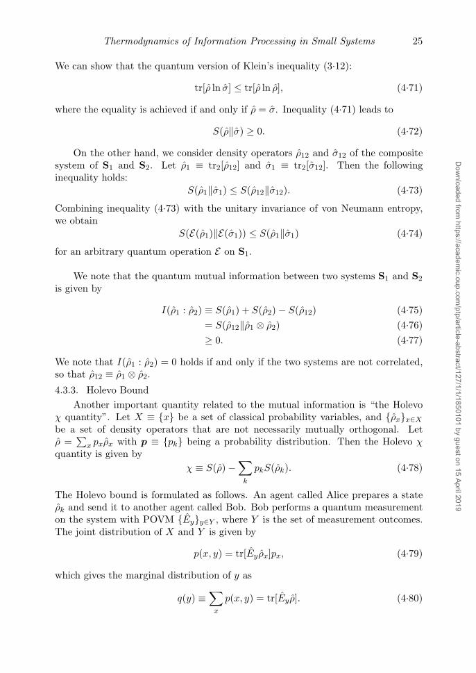
4.3.3. Holevo BoundAnother important quantity related to the mutual information is “the Holevo
χ quantity”. Let X ≡ {x} be a set of classical probability variables, and {ρx}x∈X
be a set of density operators that are not necessarily mutually orthogonal. Letρ =
∑x pxρx with p ≡ {pk} being a probability distribution. Then the Holevo χ
quantity is given byχ ≡ S(ρ) −
∑k
pkS(ρk). (4.78)
The Holevo bound is formulated as follows. An agent called Alice prepares a stateρk and send it to another agent called Bob. Bob performs a quantum measurementon the system with POVM {Ey}y∈Y , where Y is the set of measurement outcomes.The joint distribution of X and Y is given by
p(x, y) = tr[Eyρx]px, (4.79)
which gives the marginal distribution of y as
q(y) ≡∑
x
p(x, y) = tr[Eyρ]. (4.80)
Dow
nloaded from https://academ
ic.oup.com/ptp/article-abstract/127/1/1/1850101 by guest on 15 April 2019
26 T. Sagawa
Let q ≡ {q(y)}. Then the classical mutual information between X and Y is givenby
I(X : Y ) =∑x,y
p(x, y) lnp(x, y)p(x)q(y)
. (4.81)
The Holevo bound states that the classical mutual information is bounded by theHolevo χ quantity as
I(X : Y ) ≤ χ, (4.82)
which implies that the accessible information that is coded on the quantum statesis bounded by χ. We note that, from inequality (4.68), the Holevo χ quantity isbounded by the Shannon information of X as χ ≤ H(p), where the equality isachieved if and only if the supports of ρk’s are mutually orthogonal. Since the non-orthogonality of density operators characterizes their indistinguishability, we canconclude that mutual information I(X : Y ) decreases by the indistinguishability ofthe quantum states.
4.3.4. QC-Mutual InformationWe next discuss “QC-mutual information”, which will play crucial roles in
the generalizations of the second law of thermodynamics. Here, “QC” denotes“quantum-classical”; as we will see later, QC-mutual information characterizes akind of correlation between a quantum system and a classical system. The QC-mutual information was first introduced by Groenewold and Ozawa,119),120) andindependently re-introduced in Ref. 87).
We consider density operator ρ of quantum system S, and perform a quantummeasurement on it. Let {Ey}y∈Y be the POVM of the measurement, where Yis the set of measurement outcomes. The probability of obtaining y is given byp(y) = tr[Eyρ]. Let p ≡ {p(y)} and H(p) ≡ −∑y p(y) ln p(y). The QC-mutualinformation associated the POVM is then defined as
IQC ≡ S(ρ) +H(p) +∑
y
tr(√
Eyρ
√Ey ln
√Eyρ
√Ey
). (4.83)
We note that, the QC-mutual information can be rewritten as
IQC ≡ S(ρ) −∑
y
p(y)S(ρ(y)), (4.84)
whereρ(y) ≡ 1
p(y)
√Eyρ
√Ey. (4.85)
In Ref. 87), it has been shown that the QC-mutual information satisfies
0 ≤ IQC ≤ H(p). (4.86)
Here, IQC = 0 holds for all state ρ if and only if Ey is proportional to the identityoperator for every y, which means that we cannot obtain any information about thesystem by this measurement. On the other hand, IQC = H(q) for some ρ holds if
Dow
nloaded from https://academ
ic.oup.com/ptp/article-abstract/127/1/1/1850101 by guest on 15 April 2019

Thermodynamics of Information Processing in Small Systems 27
and only if Ey is the projection operator satisfying [ρ, Ey] = 0 for every y, whichmeans that the measurement on state ρ is classical and error-free.
The proof of inequality (4.86) is as follows. We first note that
−∑
y
tr(√
Eyρ
√Ey ln
√Eyρ
√Ey
)=∑
y
p(y)S(
1p(y)
√Eyρ
√Ey
)+H(p), (4.87)
where S(·) denotes the von Neumann entropy. We introduce auxiliary system Rwhich is spanned by orthonormal basis {|φy〉}y∈Y , and note that
S
(1
p(y)
√Eyρ
√Ey
)= S
(1
p(y)
√Eyρ
√Ey ⊗ |φy〉〈φy|
). (4.88)
Noting that S(L†L) = S(LL†) holds for any linear operator L, we have
−∑
y
tr(√Eyρ
√Ey ln
√Eyρ
√Ey) =
∑y
p(y)S(
1p(y)
√Eyρ
√Ey ⊗ |φy〉〈φy|
)+H(p)
=∑
y
p(y)S(
1p(y)
√ρEy
√ρ⊗ |φy〉〈φy|
)+H(p).
(4.89)
Since√ρEy
√ρ⊗ |φy〉〈φy|/p(y)’s are mutually orthogonal, we have
∑y
p(y)S(
1p(y)
√ρEy
√ρ⊗ |φy〉〈φy|
)+H(p) = S(σ), (4.90)
whereσ ≡
∑y
√ρEy
√ρ⊗ |φy〉〈φy|. (4.91)
We note that trR(σ) = ρ and trS(σ) =∑
y p(y)|φy〉〈φy| ≡ ρR hold. Therefore
−∑
y
tr(√Eyρ
√Ey ln
√Eyρ
√Ey) = S(σ1)
≤ S(ρ) + S(ρR)= S(ρ) +H(p), (4.92)
which implies IQC ≥ 0. The equality in (4.92) holds for every ρ if and only if σ canbe written as tensor product ρ ⊗ ρR for every ρ: that is, Ey is proportional to theidentity operator for all y.
We will next show that IQC ≤ H(p). We first note that
H(p) − IQC = H(p) +∑
y
p(y)S(ρ(y)) − S(ρ). (4.93)
Dow
nloaded from https://academ
ic.oup.com/ptp/article-abstract/127/1/1/1850101 by guest on 15 April 2019
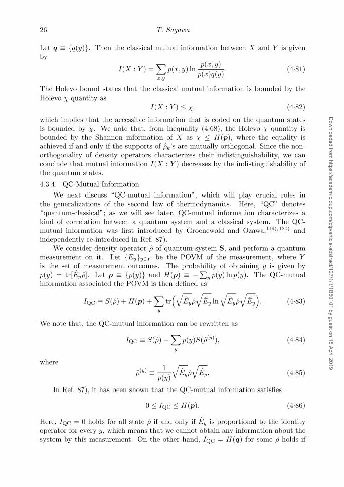
28 T. Sagawa
Let ρ′ ≡ ∑y p(y)ρ
(y) =∑
y
√Eyρ
√Ey. We make the spectral decompositions as
ρ =∑
i ri|ψi〉〈ψi| and ρ′ =∑
j sj |ψ′j〉〈ψ′
j |, where sj =∑
i ridij, and define eij ≡∑y |〈ψi|
√Ey|ψ′
j〉|2, where∑
i eij = 1 for all j and∑
j eij = 1 for all i. It followsfrom the convexity of −x lnx that S(ρ) = −∑i ri ln ri ≤ −∑j sj ln sj = S(ρ′).Therefore,
H(p) − IQC = H(p) +∑
y
p(y)S(ρ(y)) − S(ρ)
≥ H(p) +∑
k
p(y)S(ρ(y)) − S(ρ′)
≥ 0. (4.94)
The necessary and sufficient conditions that H(p) = IQC for a given ρ are:• Ey is a projection operator on the support of ρ for every y.• [ρ, Ey] = 0 for every y.
We next discuss another inequality of the QC-mutual information. Let Myi’sbe the measurement operators, which leads to an element of the POVM as Ey ≡∑
i M†yiMyi. Let pyi ≡ tr[ρM †
yiMyi] which satisfies p(y) =∑
i pyi. The correspondingQC-mutual information is given by Eq. (4.83) or (4.84). On the other hand, we definea different POVM whose elements are given by E′
yi ≡ M †yiMyi. The QC-mutual
information corresponding to POVM {E′yi} is then given by
I ′QC ≡ S(ρ) −∑
y
pyiS
(√E′
yiρ√E′
yi/pyi
)= S(ρ) −
∑y
pyiS(M †
yiρMyi/pyi
).
(4.95)Noting that ∑
i
pyi
p(y)S(MyiρM
†yi/pyi) =
∑i
pyi
p(y)S(√
ρM †yiMyi
√ρ/pyi
)
≤ S(√
ρEy
√ρ/p(y)
)= S
(√Eyρ
√Ey/p(y)
), (4.96)
we obtainIQC ≥ I ′QC. (4.97)
Inequality (4.97) implies that the QC-mutual information decreases by the coarse-graining.
We next discuss the relationship between the QC-mutual information and theHolevo χ quantity. For simplicity, we consider the case in which the measurement op-
erators are written as My =√Ey where Ek’s are the elements of the POVM. In this
case, the post-measurement state with outcome y is given by ρ(y) ≡ My ρMy/p(y),
Dow
nloaded from https://academ
ic.oup.com/ptp/article-abstract/127/1/1/1850101 by guest on 15 April 2019

Thermodynamics of Information Processing in Small Systems 29
where p(y) ≡ tr[Eyρ]. Let ρ ≡ ∑y MyρMy. Then the QC-mutual information can
be written asIQC = χ−ΔSmeas, (4.98)
whereχ ≡ S(ρ′) −
∑y
pkS(ρ(y)) (4.99)
is the Holevo χ quantity of the post-measurement states {ρ(y)}, and
ΔSmeas ≡ S(ρ′) − S(ρ) (4.100)
is the difference in the von Neumann entropy between the pre-measurement andpost-measurement states. If ΔSmeas = 0 holds, that is, if the measurement processdoes not disturb the measured system, then IQC reduces to the Holevo χ quantity.
4.3.5. Quantum-Classical CorrespondenceWe now show that the classical measurement theory discussed in §3 is a special
case of the quantum measurement theory. We write the classical probability distribu-tion as p ≡ (p[1], p[2], · · · , p[n]), where 1, 2, · · · , n denote the states of the measuredsystem. The classical distribution p corresponds to a diagonal density operatorρ ≡ diag(p1, p2, · · · , pn), where diag(· · · ) means the diagonal matrix whose diagonalelements are given by “· · · ”. On the other hand, for every measurement outcome y(= 1, 2, · · · ,m), the conditional probabilities p[y|x] (x = 1, 2, · · · , n) correspond toa diagonal measurement operator My ≡ diag(
√p[y|1],
√p[y|2], · · · ,√p[y|n]). Then
the POVM is given by Ey ≡ M †yMy = diag(p[y|1], p[y|2], · · · , p[y|n]), which com-
mutes with the measured density operator. We note that the probability of obtainingoutcome y is given by
q[y] ≡∑
x
p[y|x]p[x] = tr[Eyρ]. (4.101)
The joint distribution of x and y corresponds to
My ρM†y = diag(p[y|1]p[1], p[y|2]p[2], · · · , p[y|n]p[n]). (4.102)
Therefore we obtain the post-measurement state with outcome y:
1q[y]
MyρM†y = diag
(p[y|1]p[1]q[y]
,p[y|2]p[2]q[y]
, · · · , p[y|n]p[n]q[y]
), (4.103)
which corresponds the Bayes theorem (3.20). We note that, in the cases of classicalmeasurements, every element of a POVM is always written as Ey = M †
yMy with My
being a measurement operator. We also note that∑y
MyρM†y = ρ (4.104)
holds for classical measurement, which implies that we can neglect the effect of thedecoherence due to the measurement in the cases of classical measurements.
Dow
nloaded from https://academ
ic.oup.com/ptp/article-abstract/127/1/1/1850101 by guest on 15 April 2019
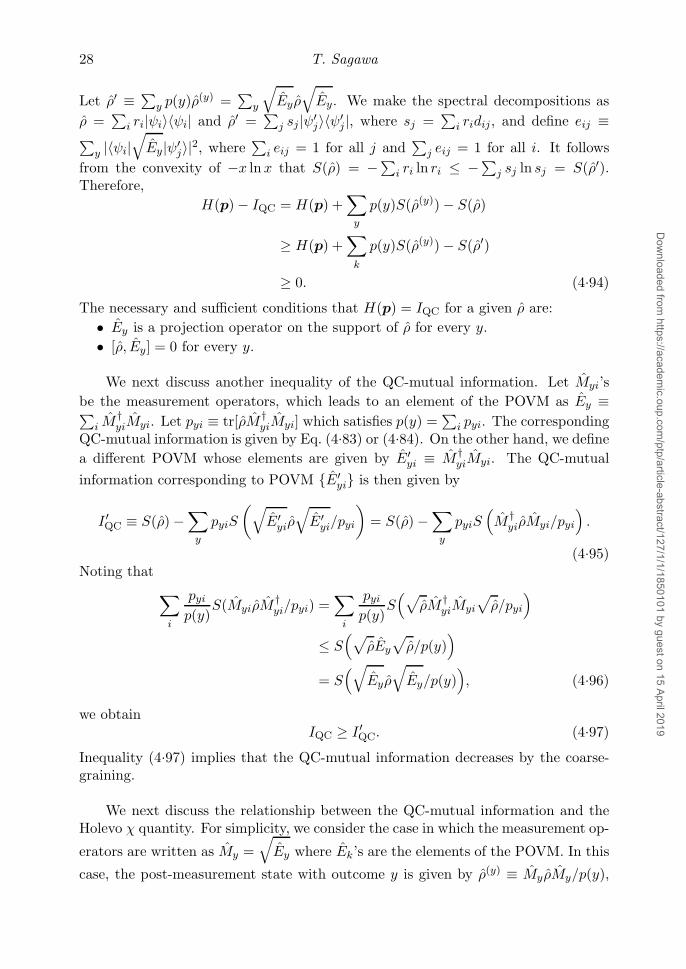
30 T. Sagawa
We next show that the QC-mutual information reduces to the classical mutualinformation in the case of the classical measurements. In this case, we have
S(ρ) = −∑
x
p[x] ln p[x] (4.105)
and
−∑
y
tr(√
Eyρ
√Ey ln
√Eyρ
√Ey
)= −
∑x,y
p[y|x]p[x] ln p[y|x]p[x]. (4.106)
Therefore IQC can be written as
IQC = −∑
y
q[y] ln q[y] −∑
x
p[x] ln p[x] +∑x,y
p[y|x]p[x] ln p[y|x]p[x], (4.107)
which is the classical mutual information.
Therefore, the arguments based on quantum theory in the following sectionsinvolve the classical cases, by regarding classical measurements and the classicalmutual information as special cases of quantum measurements and the QC-mutualinformation.
§5. Unitary proof of the second law of thermodynamics
We next review how to derive the second law of thermodynamics based on mi-croscopic dynamics. Starting with the statement of the second law, we derive itby a standard method in nonequilibrium statistical mechanics.27),33),51),121),122) Weformulate the theory such that the total system of the thermodynamic system andthe heat baths obey the unitary evolution, and assume that the initial states of theheat baths are in the canonical distribution. The reason why the second law can bederived from the reversible unitary evolution is due to the fact that we select thecanonical distributions as the initial states.
5.1. Second Law of Thermodynamics
Since the 19th century,2) the second law of thermodynamics has been establishedfor macroscopic systems. From the modern point of view, there are several expres-sions of the second law.3)–8) In particular, if a macroscopic thermodynamic systemS is in contact with a large single heat bath at temperature T = (kBβ)−1, the secondlaw for isothermal processes is formulated as follows. Suppose that the initial stateof S is in thermal equilibrium at temperature T . We then perform thermodynamicoperations on S through external parameters such as the volume of the gas. We donot assume that S is in thermal equilibrium during the operation. After that, systemS goes back to a thermal equilibrium at temperature T . In this case, the work W S
performed on S is bounded by the difference of the Helmholtz free energy ΔF S as
W S ≥ ΔF S. (5.1)
Dow
nloaded from https://academ
ic.oup.com/ptp/article-abstract/127/1/1/1850101 by guest on 15 April 2019
Thermodynamics of Information Processing in Small Systems 31
We stress that, in general, inequality (5.1) holds even if the intermediate statesof the thermodynamic operation are out of equilibrium. The equality of (5.1) isachieved if the process is quasi-static, i.e., if all of the intermediate states are inthermal equilibrium. In the case of a thermodynamic cycle, inequality (5.1) reducesto Kelvin’s principle:
W Sext ≤ 0, (5.2)
where W Sext ≡ −W S. We note that, according to thermodynamics, the Helmholtz
free energy F S and the internal energy ES are related to the thermodynamic entropySS
therm asSS
therm = β(ES − F S). (5.3)
We next suppose that thermodynamic system S can contact multi-heat baths B1,B2, · · · , Bn, at respective temperatures T1 = (kBβ1), T2 = (kBβ2), · · · , Tn = (kBβn).If the initial and final states of S are in thermal equilibrium at temperature T andthe process is a thermodynamic cycle, then the second law of thermodynamics isexpressed as the Clausius inequality:∑
m
βmQm ≤ 0, (5.4)
where Qm is the heat absorbed by S from Bm. If there are only two heat bathsBH and BL at respective temperatures TH and TL, inequality (5.4) gives the Carnotbound:
W Sext
QH=QH +QL
QH≤ 1 − TL
TH, (5.5)
where QH (QL) is the heat absorbed by S from BH (BL), and W Sext = QH + QL is
the work that is extracted from S.
In terms of statistical mechanics, thermodynamic quantities in thermal equi-librium can be calculated by using probability models. One of the most usefulprobability models is the canonical distribution:
ρScan ≡ e−βHS
ZS, (5.6)
where HS is the Hamiltonian of the system, and
ZS ≡ tr[e−βHS]. (5.7)
With the canonical distribution, free energy F S can be calculated as
F S = −kBT lnZS, (5.8)
and internal energy ES asES = tr[HSρS
can]. (5.9)
From Eqs. (5.8) and (5.9), we obtain
β(ES − F S) = −tr[ρScan ln ρS
can] ≡ S(ρScan), (5.10)
Dow
nloaded from https://academ
ic.oup.com/ptp/article-abstract/127/1/1/1850101 by guest on 15 April 2019

32 T. Sagawa
where S(· · · ) is the von Neumann entropy. Combining Eqs. (5.3) and (5.10), weobtain
SStherm = S(ρS
can), (5.11)
which implies that the thermodynamic entropy and the von Neumann entropy areequivalent in the canonical distribution. We note that, however, this equivalencerigorously holds only for the canonical distribution.
In the following arguments of this article, we sometimes assume that the initialdistribution of a thermodynamic system is in the canonical distribution, while we donot assume that any intermediate or final state is in the canonical distribution. Insuch cases, we assume the equivalence between the von Neumann entropy and thethermodynamic entropy only in the initial state.
In this section, we will discuss the following two problems:• How to prove the second law?• How to generalize the second law to microscopic systems?
We will answer theses questions by formulating the total system of the thermody-namic system and heat baths as a unitary system. The crucial assumption is thatthe total system (or at least the heat baths) is in the canonical distribution in theinitial state. This formulation is a standard method to prove the second law ofthermodynamics and the nonequilibrium equalities in nonequilibrium statistical me-chanics. Since our formulation does not involve any factor to characterize the size ofthe system, our proof can be applied to microscopic systems.
5.2. Initial Canonical Distribution with a Single Heat Bath
We first consider a quantum system that obeys a unitary evolution from time 0to τ . The Hamiltonian of the system is given by H(λ), where λ describes a set ofexternal parameters such as an applied magnetic field or the volume of the gas. Wecontrol λ from time 0 to τ with time-dependent protocol λ(t). Let Hi ≡ H(λ(0)) andHf ≡ H(λ(τ)). We define the partition functions and the Helmholtz free energieswith temperature T = (kBβ)−1corresponding to the initial and final Hamiltonians:
Zi ≡ tr[e−βHi ], Zf ≡ tr[e−βHf ], (5.12)
andFi ≡ −kBT lnZi, Ff ≡ −kBT lnZf . (5.13)
The initial state of the system is assumed to be the canonical distribution attemperature T :
ρi = ρcan,i ≡ e−βHi
Zi. (5.14)
The system evolves with the unitary evolution
U ≡ T exp(−i∫ τ
0H(λ(t)dt)
), (5.15)
Dow
nloaded from https://academ
ic.oup.com/ptp/article-abstract/127/1/1/1850101 by guest on 15 April 2019
Thermodynamics of Information Processing in Small Systems 33
where T denotes the time-ordered product. Then the final state of the system isgiven by
ρf = U ρiU†, (5.16)
which is not necessarily equal to the canonical distribution ρcan,f ≡ e−βHf/Zf .Since the von Neumann entropy S(·) is time-invariant under unitary evolutions,
we obtainS(ρi) = S(ρf). (5.17)
On the other hand, from Klein’s inequality, we have
S(ρf) ≤ −tr[ρf ln ρcan,f ], (5.18)
where the equality is achieved if and only if the final state is in the canonical distri-bution: ρf = ρcan,f . We can also show that
S(ρi) = β(tr[Hiρi] − Fi), (5.19)
because the system is initially in the canonical distribution (i.e., ρi = ρi,can), andthat
−tr[ρf ln ρcan,f ] = β(tr[Hf ρf ] − Ff). (5.20)
Therefore we obtaintr[Hf ρf ] − tr[Hiρi] ≥ Ff − Fi. (5.21)
We note that the left-hand side of (5.21) is the difference of the energies of the initialand final states. Since the system is not in contact with another heat bath, we canidentify the energy difference with the work performed on the system. Therefore, wewrite
W ≡ tr[Hf ρf ] − tr[Hiρi]. (5.22)
By defining ΔF ≡ Ff − Fi, we obtain
W ≥ ΔF, (5.23)
which is, at least formally, the second law of thermodynamics for isothermal processes.The equality in (5.23) is achieved if and only if ρi = ρi,can.
We stress that we did not assume that the final state of the system is the canon-ical distribution. In fact, we cannot say that even the temperature is well-defined inthe final state. The final free energy Ff is only formally defined by using the finalHamiltonian Hf and the initial temperature T , which is a standard formulation inmodern nonequilibrium statistical physics. Since the final state is arbitrary, inequal-ity (5.23) can be applied to an arbitrary nonequilibrium processes in which only theinitial state is in the canonical distribution; inequality (5.23) still holds even whenthe final state is far from equilibrium. We also stress that we did not assume thatthe system is large; inequality (5.23) can be applied even to small systems.
We note that the difference between the work and the free-energy change is givenby the Kullback-Leibler divergence:
W −ΔF = kBTS(ρf‖ρf,can), (5.24)
Dow
nloaded from https://academ
ic.oup.com/ptp/article-abstract/127/1/1/1850101 by guest on 15 April 2019

34 T. Sagawa
which implies that the dissipation W − ΔF is given by the gap between the finalstate and the canonical distribution.
The purpose of this article is to consider small systems which is in contact withlarge heat bath(s). To explicitly take into account the effect of a heat bath, we dividethe above system into two: small system S and large heat bath B. In this situation,we write the total Hamiltonian as
H(λ, c) = HS(λ) + HSB(c) + HB, (5.25)
where HS(λ) is the Hamiltonian of S, HSB(c) is the interaction Hamiltonian betweenS and B, and HB(λ) is the Hamiltonian of B. We assume that S can be controlledthrough external parameters λ. In addition, we assume that the interaction betweenS and B can also be controlled by external parameters c. This assumption is notunrealistic: we can control the strength of the interaction by, for example, using anadiabatic wall on S. Moreover, in some special setups, we can use the dynamicaldecoupling to control the strength of the interaction. Let Hi ≡ H(λ(0), c(0)), Hf ≡H(λ(τ), c(τ)), HS
i ≡ HS(λ(0)), HSf ≡ H(λ(τ)), HSB
i ≡ HSB(c(0)), and HSBf ≡
HSB(c(τ)). We define the partition functions and the Helmholtz free energies
ZSi ≡ tr[e−βHS
i ], ZSf ≡ tr[e−βHS
f ], (5.26)
andF S
i ≡ −kBT lnZSi , F
Sf ≡ −kBT lnZS
f . (5.27)
If the initial and final interactions are zero, i.e., HSBi = HSB
f = 0 holds, theninequality (5.21) reduces to
W S ≥ ΔF S, (5.28)
whereW S ≡W ≡ tr[Hf ρf ] − tr[Hiρi] (5.29)
is the work performed on S, and ΔF S ≡ F Sf − F S
i is the free-energy difference of S.We note that W S = W holds because the total energy difference of S and B is theenergy input through external parameter, which is the work (see also Fig. 6).
If the initial and final interactions are weak enough, inequality (5.28) holdsapproximately.
Inequality (5.28) is better than (5.23) as the microscopic foundation of the secondlaw of thermodynamics (5.1), because the former takes into account the effect of a
Fig. 6. Energy balance of the total system of S and B.
Dow
nloaded from https://academ
ic.oup.com/ptp/article-abstract/127/1/1/1850101 by guest on 15 April 2019
Thermodynamics of Information Processing in Small Systems 35
heat bath. In fact, in the original second law of thermodynamics, a macroscopicsystem obeys an isothermal process with a large heat bath, and both the initial andfinal states of the system are assumed to be in thermal equilibrium. If S and B arelarge enough and the system is relaxed to the thermal equilibrium in the final state,inequality (5.28) is expected to lead to the original second law of thermodynamics.However, we note that, inequality (5.28) is more general than the original secondlaw of thermodynamics: in (5.28), we did not assume that S is large nor that thefinal state of S is in the canonical distribution.
We note that, if the initial and final interactions are zero nor weak, we canformally introduce the effective free energies55) as
F Si ≡ Fi − FB, F S
f ≡ Ff − FB, (5.30)
where FB ≡ −kBT ln tr[e−βHB] is the free energy of B. Then inequality (5.23)
trivially reduces toW S ≥ ΔF S, (5.31)
where ΔF S ≡ F Sf − F S
i . However, in the following, we assume that HSBi = HSB
f = 0holds for simplicity.
5.3. General Situations with Multi-Heat Baths
We next consider a thermodynamic process of system S that can contact heatbaths B1, B2, · · · , Bn, at respective temperatures T1 = (kBβ1), T2 = (kBβ2), · · · ,Tn = (kBβn). We assume that the total of S and Bm’s obeys a unitary evolution.The total Hamiltonian can be written as
H(λ, {cm}) = HS(λ) +n∑
m=1
(HSBm(cm) + HBm), (5.32)
where HS(λ) is the Hamiltonian of S, HSBm(cm) is the interaction Hamiltonian be-tween S and Bm, and HBm is the Hamiltonian of Bm. Here, λ describes controllableexternal parameters, and cm describes external parameters to control the interactionbetween S and Bm.
We consider a time evolution from 0 to τ , and assume that HSBm(cm(0)) =HSBm(cm(τ)) = 0 holds for all m. We write HS(λ(0)) ≡ HS
i , HS(λ(τ)) ≡ HSf ,
H(λ(0), {cm(0)}) ≡ Hi, and H(λ(τ), {cm(0)}) ≡ Hf .We assume that the initial state of the total system is given by
ρi ≡ ρS ⊗ ρB1can ⊗ · · · ⊗ ρBn
can, (5.33)
where ρS is an arbitrary initial state of S, and
ρBmcan ≡ e−βmHBm
ZBm, (5.34)
is the canonical distribution with ZBm ≡ tr[e−βHBm ]. We write the free energies ofthe heat baths as FBm ≡ kBTm lnZBm . We note that Eq. (5.33) is consistent withthe assumption that HSBm(cm(0)) = HSBm(cm(τ)) = 0 holds for all m.
Dow
nloaded from https://academ
ic.oup.com/ptp/article-abstract/127/1/1/1850101 by guest on 15 April 2019
36 T. Sagawa
The unitary evolution of the total system is given by
U ≡ T exp(−i∫ τ
0H(λ(t), {cm(t)})dt
), (5.35)
which leads to the final stateρf ≡ U ρiU
†. (5.36)
We write ρS ≡ trB1···Bn [ρf ].Due to the unitary invariance of the von Neumann entropy, we obtain
S(ρi) = S(ρf). (5.37)
On the other hand, we have
S(ρi) = S(ρSi ) +
∑m
βm
(tr[ρiH
Bm ] − FBm
). (5.38)
From Klein’s inequality, we also have
S(ρf) ≥ tr[ρf ln(ρSf ⊗ ρB1
can ⊗ · · · ⊗ ρBncan)] (5.39)
= S(ρSf ) +
∑m
βm
(tr[ρfH
Bm ] − FBm
), (5.40)
where we used −tr[ρf ln ρSf ] = S(ρS
f ). Therefore we obtain
S(ρSf ) − S(ρS
i ) ≥∑m
βmQm, (5.41)
whereQm ≡ tr[ρiH
Bm ] − tr[ρfHBm ] (5.42)
is the heat that is absorbed by system S from heat bath Bm. Inequality (5.41) is themain result of this section. We stress that inequality (5.41) holds for arbitrary initialand final states of S (i.e., ρS
i and ρSf ); in fact, we have only assumed that the initial
distributions of the heat baths are in the canonical distribution. Inequality (5.41)can be regarded as a generalization of Clausius’ inequality (5.4) to nonequilibriuminitial and final distributions.
We consider inequality (5.41) for special cases.
Nonequilibrium steady state. We first consider a simple case in which system Sis in contact with two heat baths TH = (kBβH)−1 and TL = (kBβL)−1 with TH > TL,and S is in a nonequilibrium steady state with a constant heat flow QH = −QL ≡ Q.Since S is in a steady state, we may assume S(ρS
i ) = S(ρSf ). Therefore inequality
(5.41) reduces to(βH − βL)Q ≤ 0, (5.43)
and therefore Q ≤ 0, implying that the heat flows from the hot bath to the cold one.
Dow
nloaded from https://academ
ic.oup.com/ptp/article-abstract/127/1/1/1850101 by guest on 15 April 2019
Thermodynamics of Information Processing in Small Systems 37
Isothermal process. We next consider the case in which there is a single heatbath at temperature T = (kBβ)−1. In this case, inequality (5.41) reduces to
S(ρSf ) − S(ρS
i ) ≥ βQ. (5.44)
We then assume that the initial state of S is the canonical distribution as
ρSi = ρS
can,i ≡e−βHS
i
ZSi
, (5.45)
where ZSi ≡ tr[e−βHS
i ]. We also introduce notations as
F Si ≡ −kBT lnZS
i , (5.46)
e−βHSf
ZSf
, ZSf ≡ tr[e−βHS
f ], F Sf ≡ −kBT lnZS
f . (5.47)
From Klein’s inequality, we obtain
S(ρSf ) − S(ρS
i ) ≤ β(ΔES −ΔF S), (5.48)
whereΔES ≡ tr[HS
f ρSf ] − tr[HS
i ρSi ] (5.49)
is the internal-energy difference of S, and
ΔF S ≡ F Sf − F S
i . (5.50)
From inequalities (5.44) and (5.48), we have
ΔES −ΔF S ≥ Q. (5.51)
On the other hand, the first law of thermodynamics holds as
ΔES = Q+W S, (5.52)
where W S is the work performed on the system, which is given by Eq. (5.29). There-fore we reproduce inequality (5.28).
With multi-heat baths. We next consider the case in which there are multi-heatbaths. We again assume that the initial state of S is the canonical distribution attemperature T = (kBβ)−1. While T is arbitrary in general, we can assume that Tis equal to Tm if S is initially in contact only with Bm. By using inequality (5.48),inequality (5.41) leads to
β(ΔES −ΔF S) ≥∑m
βmQm. (5.53)
In the case of a thermodynamic cycle with ΔES = ΔF S = 0, we obtain∑m
βmQm ≤ 0, (5.54)
Dow
nloaded from https://academ
ic.oup.com/ptp/article-abstract/127/1/1/1850101 by guest on 15 April 2019
38 T. Sagawa
which is Clausius’ inequality (5.4). In particular, if there are two heat baths attemperatures TH = (kBβH)−1 and TL = (kBβL)−1 with TH > TL, we obtain
W Sext
QH≤ 1 − TH
TL, (5.55)
where W Sext = QH−QL is the work that is extracted from the cycle. Inequality (5.55)
implies the Carnot bound.
§6. Second law with feedback control
We now proceed to the main part of this article. In this section, we review ageneralized second law with a quantum measurement and feedback control, whichhas been derived in Ref. 87). In §6.1, we discuss the lower bound of the entropydifference by feedback control. Based on it, we discuss a generalized second law ofthermodynamics with feedback control in §6.2.
6.1. Entropy Inequality
We first discuss the entropy balance of a quantum system that obeys a quantummeasurement and feedback in addition to unitary evolutions. Let ρi be an arbitraryinitial density operator of a finite-dimensional quantum system, which evolves asfollows.
Step 1: Unitary evolution. From time 0 to t1, the system undergoes unitaryevolution Ui. At time t1, the density operator is given by ρ1 = UiρiU
†i .
Step 2: Measurement. From time t1 to t2, we perform a quantum measurementon the system. We assume that the measurement is described by measurementoperators {Mk} with k’s being measurement outcomes, which leads to POVM
Ek ≡ M †kMk. (6.1)
We obtain each outcome k with probability
pk = tr(Ekρ1). (6.2)
Here we assumed that every single measurement operator corresponds a single mea-surement outcome as Eq. (6.1). Let p ≡ {pk}. The post-measurement state corre-sponding to outcome k is given by
ρ(k)2 =
1pkMkρ1M
†k , (6.3)
and the ensemble average is given by
ρ2 =∑
k
pkρ(k)2 =
∑k
Mkρ1M†k . (6.4)
Dow
nloaded from https://academ
ic.oup.com/ptp/article-abstract/127/1/1/1850101 by guest on 15 April 2019
Thermodynamics of Information Processing in Small Systems 39
Step 3: Feedback control. From t2 to t3, we perform feedback control; the cor-responding unitary operator Uk depends on measurement outcome k. The post-feedback state corresponding to outcome k is given by
ρ(k)3 = Ukρ
(k)2 U †
k =1pkUkMkρ1M
†kU
†k , (6.5)
and the ensemble average is given by
ρ(k)3 ≡
∑k
pkUkρ(k)2 U †
k =∑
k
UkMkρ1M†kU
†k . (6.6)
Step 4: Unitary evolution. After the feedback, from time t3 to τ , the systemevolves according to unitary operator Uf which is independent of outcome k. Thefinal state is ρf = Uf ρ3U
†f .
The entire time evolution is then given by
ρf = E(ρi) ≡∑
k
Uf UkMkUiρiU†i M
†kU
†kU
†f . (6.7)
The difference in the von Neumann entropy S between the initial and final statescan be bounded as follows:
S(ρi) − S(ρf)=S(ρ1) − S(ρ3)
≤S(ρ1) −∑
k
pkS(ρ(k)3 )
=S(ρ1) −∑
k
pkS(ρ(k)2 )
=S(ρ1) +∑
k
tr
⎛⎝√Ekρ1
√Ek ln
√Ekρ1
√Ek
pk
⎞⎠
=S(ρ1) +H(p) +∑
k
tr(√
Ekρ1
√Ek ln
√Ekρ1
√Ek
), (6.8)
where H(p) ≡ −∑k pk ln pk is the Shannon information obtained by the measure-ment. Note that in deriving the inequality (6.8), we used the convexity of the vonNeumann entropy, i.e. S(
∑k pkρ
(k)3 ) ≥ ∑k pkS(ρ(k)
3 ). From the definition (4.83) ofQC-mutual information, we obtain
S(ρi) − S(ρf) ≤ IQC, (6.9)
where the equality is achieved if and only if all of ρ(k)3 ’s are the same. Intuitively
speaking, this condition means that the feedback control is perfect, i.e., we used allthe obtained information by feedback control.
Dow
nloaded from https://academ
ic.oup.com/ptp/article-abstract/127/1/1/1850101 by guest on 15 April 2019
40 T. Sagawa
We note that Nielsen et al.86) have derived inequality S(ρi) − S(ρf) ≤ S(ρi, E),where S(ρi, E) is the entropy exchange. The entropy exchange depends on the totalprocess E including the feedback process. On the other hand, our inequality (6.9) isbounded by IQC which does not depend on the feedback process, but only dependson the pre-measurement state and the POVM.
6.2. Generalized Second Laws
We now consider the energetics of feedback control on thermodynamic systems,in terms of the work, the heat, and the free energy. We consider a thermodynamicprocess of system S which can be in contact with heat baths B1, B2, · · · , Bn,at respective temperatures T1 = (kBβ1), T2 = (kBβ2), · · · , Tn = (kBβn). In thefollowing, we use the same notations as in §5.2.
We assume that the total system of S and heat baths Bm obeys a unitaryevolution except for the process of a measurement. Apart from the measurementapparatus, the total Hamiltonian can be written as
H(λ, {cm}) = HS(λ) +n∑
m=1
(HSBm(cm) + HBm). (6.10)
For simplicity of notations, we write λ ≡ (λ, {cm}). We assume that the initial stateof the total system is given by
ρi ≡ ρSi ⊗ ρB1
can ⊗ · · · ⊗ ρBncan, (6.11)
where ρSi is an arbitrary initial state of S. The total density operator evolves as
described in Step 1 to 5 in the previous subsection, which corresponds to the presentsetup as follows.
Step 1: From time 0 to t1, the unitary operator is given by
Ui = T exp(−i∫ t1
0H(λ(t))dt
). (6.12)
Step 2: From time t1 to t2, we perform a measurement. While we perform itonly on S, the corresponding measurement operators can be extended to the totalsystem, which are described by Mk’s.
Step 3: From time t2 to t3, we perform feedback control in which the controlprotocol of λ depends on measurement outcome k as λ(t; k). The unitary evolutionis then given by
Uk = T exp(−i∫H(λ(t; k))dt
). (6.13)
Step 4: From time t3 to τ , the total system obeys the unitary evolution
Uf = T exp(−i∫ τ
t3
H(λ(t))dt). (6.14)
Dow
nloaded from https://academ
ic.oup.com/ptp/article-abstract/127/1/1/1850101 by guest on 15 April 2019
Thermodynamics of Information Processing in Small Systems 41
To transform inequality (6.9) to energetic inequalities, we can apply the sameargument as in §5.2. First of all, inequality (5.37) is replaced by inequality (6.9) inthe presence of feedback control. We then obtain
S(ρSf ) − S(ρS
i ) ≥∑m
βmQm − IQC, (6.15)
which is a generalization of inequality (5.41) to the situation in which the system issubject to feedback control. Inequality (6.15) is a little generalization of the mainresult of Ref. 87).
If there is a single heat bath and the initial distribution of S is a canonicaldistribution, (6.15) reduces to
W S ≥ ΔF S − kBTIQC, (6.16)
where W S is given by Eq. (5.29). Inequality (6.16) is a generalization of inequality(5.44) to feedback-controlled processes, which is one of the main results in Ref. 87).By introducing notation W S
ext ≡ −W S, inequality (6.16) can be rewritten as
W Sext ≤ −ΔF S + kBTIQC. (6.17)
Inequality (6.17) implies that we can extract work greater than −ΔF S froma single heat bath with feedback control, but that we cannot extract work largerthan −ΔF S + kBTIQ. If IQC = 0, inequality (6.17) reduces to (5.28). On the otherhand, in the case of a classical and error-free measurement, inequality (6.17) becomesWext ≤ −ΔF S + kBTH(p).
The upper bound of inequality (6.17) can be achieved with the Szilard engine10)
in which IQC = H(p) = ln 2, Wext = ln 2, and ΔF S = 0 hold. In fact, in the case ofthe Szilard engine, the expansion is quasi-static and the post-feedback state is inde-pendent of the measurement outcomes. Moreover, as shown in Ref. 88), the upperbound of inequality (6.17) can be achieved for any quantum measurement satisfyingEq. (6.1). Some models that achieves the upper bound of (6.17) are discussed inRefs. 113) and 114) for classical stochastic systems.
If there are multi-heat baths and the initial state of S is the canonical distributionat temperature T = (kBβ)−1, inequality (6.17) leads to another main result of thissection:
β(ΔES −ΔF S) ≥∑m
βmQm − IQC, (6.18)
which is a generalization of inequality (5.53). Inequality (6.18) represents the secondlaw of thermodynamics with multi-heat baths in the presence of a feedback con-trol, where the effect of the feedback control is described by the last term. For athermodynamic cycle with ΔES = 0, and ΔF S = 0, inequality (6.18) reduces to ageneralized Clausius inequality
n∑m=1
Qm
Tm≤ IQC. (6.19)
Dow
nloaded from https://academ
ic.oup.com/ptp/article-abstract/127/1/1/1850101 by guest on 15 April 2019
42 T. Sagawa
In particular, in the case of a thermodynamic cycle with two heat baths withfeedback control, we obtain
W Sext ≤
(1 − TL
TH
)QH + kBTLIQ, (6.20)
which is a generalization of Carnot’s bound (5.55). Inequality (6.20) implies that theupper bound for the efficiency of heat cycles becomes larger than that of the Carnotcycle with feedback control.
We can achieve the upper bound of (6.20) by performing a Szilard-type operationduring an isothermal process of the one-molecule Carnot cycle. If we perform themeasurement and feedback in the same scheme as the Szilard engine during theisothermal process at temperature TL, we can extract the work of W S
ext = (1 −TL/TH)QH+kBTL ln 2 in the total process. Moreover, if we perform the measurementand feedback in the same scheme as the Szilard engine during the isothermal processat temperature TH, we can also obtain the same bound: W S
ext = (1 − TL/TH)(QH −kBTH ln 2) + kBTH ln 2 = (1 − TL/TH)QH + kBTL ln 2.
§7. Thermodynamics of memories
In the previous section, we considered a thermodynamic system that is measuredand controlled by Maxwell’s demon. In this section, in line with Ref. 97), we reviewthe thermodynamic properties of the demon itself, which is regarded as a memorythat stores the measurement outcomes. For simplicity, we consider the case in whichthere is a single heat bath. We also discuss the resolution of the paradox of Maxwell’sdemon.
7.1. Formulation of Memory
We first formulate a memory M that stores measurement outcomes. We notethat the “memory” may include the measurement apparatus that directly interactswith a measured system.
Let HM be the Hilbert space corresponding to M. We decompose HM intomutually orthogonal subspaces HM
k (k = 0, 1, 2, · · · , N), where the k’s describe themeasurement outcomes. HM is written as the direct sum of HM
k ’s as
HM =⊕
k
HMk . (7.1)
Outcome “k” is stored in M if the support of the density operator of the memory be-longs to HM
k . We note that the classical outcomes (i.e., k’s) can be distinguished eachother when they are stored in M, because HM
k ’s are mutually orthogonal. Therefore,the assumption of the orthogonality is crucial for M to work as a memory that storesclassical outcomes. We assume that M has a pre-fixed standard state, and that Mis in the standard state before a measurement. We assume that k = 0 correspondsto the standard state of M.
The total Hamiltonian of M, denoted as HM, can also be written as the direct
Dow
nloaded from https://academ
ic.oup.com/ptp/article-abstract/127/1/1/1850101 by guest on 15 April 2019
Thermodynamics of Information Processing in Small Systems 43
sum of sub-Hamiltonians:HM ≡
∑k
HMk , (7.2)
where the support of HMk is in HM
k for every k. Let the spectral decomposition ofHM
k be HMk ≡∑i εki|εki〉〈εki|, where {|εki〉}i is an orthonormal basis set of HM
k .The conditional canonical distribution at temperature T = (kBβ)−1 under the
condition of outcome “k” is given by
ρMcan,k ≡ e−βHM
k
Zk, (7.3)
where ZMk ≡ tr[exp(−βHM
k )]. The corresponding Helmholtz free energy of M with“k” is given by
FMk ≡ −kBT lnZM
k . (7.4)
7.2. Erasure Process
We consider the following process for the information erasure in the presence ofa single heat bath at temperature T = (kBβ)−1. The pre-erasure state means thepost-measurement state, in which the memory stores the information of the measuredsystem. In the pre-erasure state, M stores outcome “k” with probability pk. Wedefine p ≡ {pk}. The Shannon information corresponding to the pre-erasure state isgiven by
H(p) ≡ −∑
k
pk ln pk. (7.5)
We assume that, before the information erasure, the state of M under the conditionof “k” is in the canonical distribution ρcan
k , and that the total pre-erasure state ofM is given by
ρMi ≡
∑k
pkρMcan,k. (7.6)
We stress that memory M should be able to store an arbitrary probability dis-tribution {pk}, which is the most important necessary property for M to fulfill thefunction of a memory. For example, if the measurement is error-free, {pk} is deter-mined only by the state of the measured system. In general, {pk} is independentof the structure of the memory, while Fk’s are determined by the structure of thememory.
Let HB be the Hilbert space corresponding to the heat bath B. We assume thatB is initially in the canonical distribution, which is given by ρB
can ≡ exp(−βHB)/ZB,where HB is the Hamiltonian of B and ZB ≡ tr[exp(−βHB)] is the partition function.We also assume that the initial states of M and B are not correlated, and that theinitial state of the total system is given by
ρMBi ≡ ρM
i ⊗ ρBcan. (7.7)
We consider the erasure process from t = 0 to t = τ . During the erasure process,we change the Hamiltonian of M with a protocol which need to be independent of
Dow
nloaded from https://academ
ic.oup.com/ptp/article-abstract/127/1/1/1850101 by guest on 15 April 2019
44 T. Sagawa
k. The total Hamiltonian at time t then is given by
HMB(t) = HM(t) + H int(t) + HB, (7.8)
where H int(t) is the interaction Hamiltonian between M and B. We assume thatHM(0) = HM(τ) = HM and H int(0) = H int(τ) = 0, which is consistent withEq. (7.7). The time evolution of the total system from time 0 to τ is then givenby the unitary operator U ≡ T exp(−i
∫HMB(t)dt), which gives the post-erasure
state of the total systemsρMBf = U ρMB
i U †. (7.9)
We define ρBf ≡ trM[ρMB
f ] and ρMf ≡ trB[ρMB
f ]. After the information erasure, thestate of M is in the standard state with unit probability. In other words, the supportof ρMB
f is in HM0 ⊗ HB with unit probability.
We now derive the minimal energy cost that is needed for the erasure process.From the general second law (5.41), we obtain
S(ρMf ) − S(ρM
i ) ≥ βQMeras, (7.10)
whereQM
eras ≡ tr[HBρBcan] − tr[HBρB
f ] (7.11)
is the heat that is absorbed in M during the erasure process. On the other hand,S(ρM
i ) can be decomposed as
S(ρMi ) =
∑k
pkS(ρMcan,k) +H(p), (7.12)
because ρMcan,k’s are mutually orthogonal. We then obtain
S(ρMf ) −
∑k
pkS(ρMcan,k) −H(p) ≥ βQM
eras. (7.13)
We note thatS(ρM
can,k) = β(tr[HMk ρ
Mcan,k] − FM
k ) (7.14)
holds. On the other hand, from Klein’s inequality, we have
S(ρMf ) ≤ −tr[ρM
f ln ρMcan,0] = β(tr[HM
0 ρMf ] − FM
0 ). (7.15)
Therefore we obtain
−ΔFMeras +ΔEM
eras − kBTH(p) ≥ QMeras, (7.16)
whereΔFM
eras ≡ FM0 −
∑k
pkFMk (7.17)
is the difference of the averaged free energies of M, and
ΔEMeras ≡ tr[HM
0 ρMf ] −
∑k
pktr[HMk ρ
Mcan,k] (7.18)
Dow
nloaded from https://academ
ic.oup.com/ptp/article-abstract/127/1/1/1850101 by guest on 15 April 2019
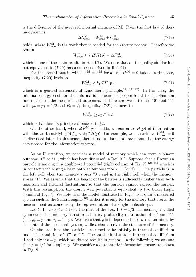
Thermodynamics of Information Processing in Small Systems 45
is the difference of the averaged internal energies of M. From the first law of ther-modynamics,
ΔEMeras = WM
eras +QMeras (7.19)
holds, where WMeras is the work that is needed for the erasure process. Therefore we
obtainWM
eras ≥ kBTH(p) +ΔFMeras, (7.20)
which is one of the main results in Ref. 97). We note that an inequality similar butnot equivalent to (7.20) has also been derived in Ref. 94).
For the special case in which FM0 = FM
k for all k, ΔFM = 0 holds. In this case,inequality (7.20) leads to
WMeras ≥ kBTH(p), (7.21)
which is a general statement of Landauer’s principle.14),89),92) In this case, theminimal energy cost for the information erasure is proportional to the Shannoninformation of the measurement outcomes. If there are two outcomes “0” and “1”with p0 = p1 = 1/2 and F0 = f1, inequality (7.21) reduces to
WMeras ≥ kBT ln 2, (7.22)
which is Landauer’s principle discussed in §2.On the other hand, when ΔFM �= 0 holds, we can erase H(p) of information
with the work satisfying WMeras < kBTH(p). For example, we can achieve WM
eras = 0as discussed later. In this sense, there is no fundamental lower bound of the energycost needed for the information erasure.
As an illustration, we consider a model of memory which can store a binaryoutcome “0” or “1”, which has been discussed in Ref. 97). Suppose that a Brownianparticle is moving in a double-well potential (right column of Fig. 7),13),14) which isin contact with a single heat bath at temperature T = (kBβ)−1. The particle is inthe left well when the memory stores “0”, and in the right well when the memorystores “1”. We assume that the height of the barrier is sufficiently higher than bothquantum and thermal fluctuations, so that the particle cannot exceed the barrier.With this assumption, the double-well potential is equivalent to two boxes (rightcolumn of Fig. 7). We note that the model illustrated in Fig. 7 is not for a measuredsystem such as the Szilard engine;10) rather it is only for the memory that stores themeasurement outcome using the representation of a single-molecule gas.
Let t : 1− t (0 < t < 1) be the ratio of the box. If t = 1/2, the memory is calledsymmetric. The memory can store arbitrary probability distribution of “0” and “1”(i.e., p0 ≡ p and p1 ≡ 1−p). We stress that p is independent of t; p is determined bythe state of the measured system, while t characterizes the structure of the memory.
On the each box, the particle is assumed to be initially in thermal equilibriumunder the condition of “0” or “1”. The total initial state is in thermal equilibriumif and only if t = p, which we do not require in general. In the following, we assumethat p = 1/2 for simplicity. We consider a quasi-static information erasure as shownin Fig. 8.
Dow
nloaded from https://academ
ic.oup.com/ptp/article-abstract/127/1/1/1850101 by guest on 15 April 2019
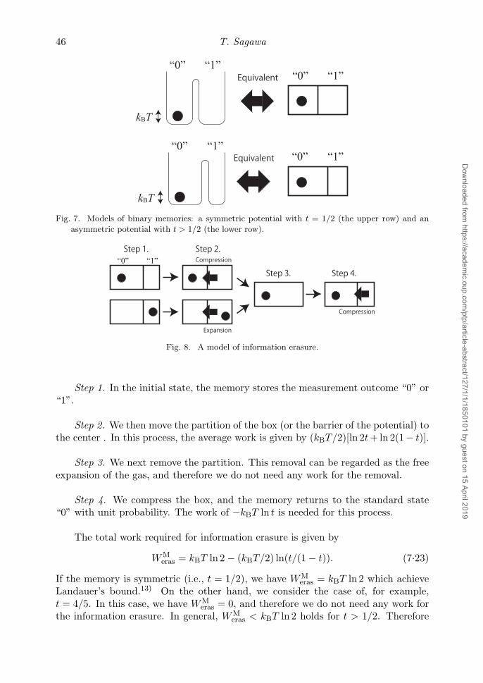
46 T. Sagawa
Fig. 7. Models of binary memories: a symmetric potential with t = 1/2 (the upper row) and an
asymmetric potential with t > 1/2 (the lower row).
Fig. 8. A model of information erasure.
Step 1. In the initial state, the memory stores the measurement outcome “0” or“1”.
Step 2. We then move the partition of the box (or the barrier of the potential) tothe center . In this process, the average work is given by (kBT/2)[ln 2t+ ln 2(1− t)].
Step 3. We next remove the partition. This removal can be regarded as the freeexpansion of the gas, and therefore we do not need any work for the removal.
Step 4. We compress the box, and the memory returns to the standard state“0” with unit probability. The work of −kBT ln t is needed for this process.
The total work required for information erasure is given by
WMeras = kBT ln 2 − (kBT/2) ln(t/(1 − t)). (7.23)
If the memory is symmetric (i.e., t = 1/2), we have WMeras = kBT ln 2 which achieve
Landauer’s bound.13) On the other hand, we consider the case of, for example,t = 4/5. In this case, we have WM
eras = 0, and therefore we do not need any work forthe information erasure. In general, WM
eras < kBT ln 2 holds for t > 1/2. Therefore
Dow
nloaded from https://academ
ic.oup.com/ptp/article-abstract/127/1/1/1850101 by guest on 15 April 2019

Thermodynamics of Information Processing in Small Systems 47
Landauer’s principle for information erasure is valid for a symmetric double-wellpotential, but not for an asymmetric one. We note that the proof of WM
eras ≥ kBT ln 2using statistical mechanics in Refs. 89) and 92) is valid only for the symmetric case.We also note that another asymmetric memory has also been discussed in Ref. 93).
7.3. Measurement Process
We next consider the measurement processes. Suppose that memory M performsa measurement on a measured system S, and stores outcome “k” with probabilitypk. We assume that the memory is in contact with heat bath BM at temperatureT = (kBβ)−1. On the other hand, during the measurement, measured system Sadiabatically evolves or is in contact with a different heat bath, denoted as BS,which is different from BM. The latter assumption corresponds to the conditionthat the thermal noises on M and S are independent. For example, two colloidalparticles, whose Langevin noises are independent, may satisfy this condition, evenwhen they are actually in the same water. The total Hamiltonian is then given by
Htot(t) = HM(t) + HMBM(t) + HBM + HM(t) + HS(t) + HSBS(t) + HBS + HMS(t),(7.24)
where HMS(t) describes the interaction between M and S for the measurement (seealso Fig. 9). We assume that HM(0) = HM(τ) = HM and HMBM(0) = HMBM(τ) =HMS(0) = HMS(τ) = 0 hold.
We consider the following measurement process.
Step 1: Initial state. The initial state of M is in the standard state “0”; weassume that the initial state of M is the conditional canonical distribution under thecondition that the support of the density operator is in HM
0 . Then the initial densityoperator of the total system is given by
ρtoti = ρM
can,0 ⊗ ρBMcan ⊗ ρSBS , (7.25)
where ρBMcan is the initial canonical distribution of BM, and ρSBS is the initial density
operator of S + BS . We stress that, in this section, we do not put any assumptionon ρSBS .
Fig. 9. A schematics of the interactions of the total system.
Dow
nloaded from https://academ
ic.oup.com/ptp/article-abstract/127/1/1/1850101 by guest on 15 April 2019
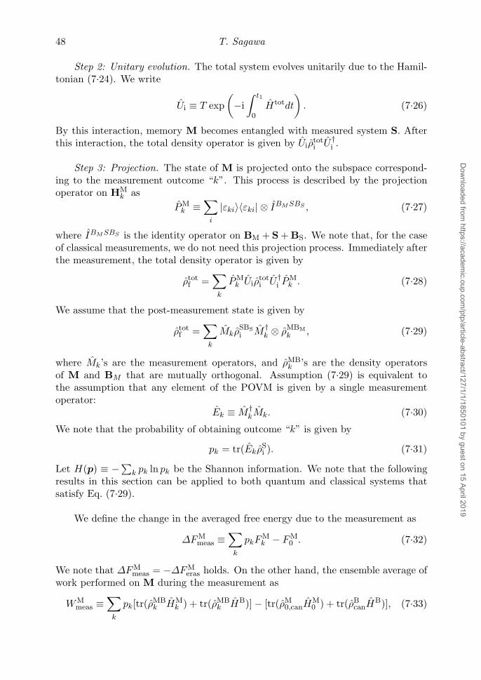
48 T. Sagawa
Step 2: Unitary evolution. The total system evolves unitarily due to the Hamil-tonian (7.24). We write
Ui ≡ T exp(−i∫ t1
0Htotdt
). (7.26)
By this interaction, memory M becomes entangled with measured system S. Afterthis interaction, the total density operator is given by Uiρ
toti U †
i .
Step 3: Projection. The state of M is projected onto the subspace correspond-ing to the measurement outcome “k”. This process is described by the projectionoperator on HM
k asPM
k ≡∑
i
|εki〉〈εki| ⊗ IBM SBS , (7.27)
where IBMSBS is the identity operator on BM + S + BS. We note that, for the caseof classical measurements, we do not need this projection process. Immediately afterthe measurement, the total density operator is given by
ρtotf =
∑k
PMk Uiρ
toti U †
i PMk . (7.28)
We assume that the post-measurement state is given by
ρtotf =
∑k
MkρSBSi M †
k ⊗ ρMBMk , (7.29)
where Mk’s are the measurement operators, and ρMBk ’s are the density operators
of M and BM that are mutually orthogonal. Assumption (7.29) is equivalent tothe assumption that any element of the POVM is given by a single measurementoperator:
Ek ≡ M †kMk. (7.30)
We note that the probability of obtaining outcome “k” is given by
pk = tr(EkρSi ). (7.31)
Let H(p) ≡ −∑k pk ln pk be the Shannon information. We note that the followingresults in this section can be applied to both quantum and classical systems thatsatisfy Eq. (7.29).
We define the change in the averaged free energy due to the measurement as
ΔFMmeas ≡
∑k
pkFMk − FM
0 . (7.32)
We note that ΔFMmeas = −ΔFM
eras holds. On the other hand, the ensemble average ofwork performed on M during the measurement as
WMmeas ≡
∑k
pk[tr(ρMBk HM
k ) + tr(ρMBk HB)] − [tr(ρM
0,canHM0 ) + tr(ρB
canHB)], (7.33)
Dow
nloaded from https://academ
ic.oup.com/ptp/article-abstract/127/1/1/1850101 by guest on 15 April 2019
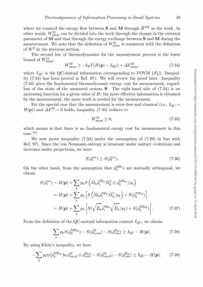
Thermodynamics of Information Processing in Small Systems 49
where we counted the energy flow between S and M through HSM as the work. Inother words, WM
meas can be divided into the work through the change in the externalparameter of M and that through the energy exchange between S and M during themeasurement. We note that the definition of WM
meas is consistent with the definitionof W S in the previous section.
The second law of thermodynamics for the measurement process is the lowerbound of WM
meas:WM
meas ≥ −kBT (H(p) − IQC) +ΔFMmeas, (7.34)
where IQC is the QC-mutual information corresponding to POVM {Ek}. Inequal-ity (7.34) has been proved in Ref. 97). We will review the proof later. Inequality(7.34) gives the fundamental thermodynamic energy cost for measurement, regard-less of the state of the measured system S. The right-hand side of (7.34) is anincreasing function for a given value of H; the more effective information is obtainedby the measurement, the more work is needed for the measurement.
For the special case that the measurement is error-free and classical (i.e., IQC =H(p)) and ΔFM = 0 holds, inequality (7.34) reduces to
WMmeas ≥ 0, (7.35)
which means is that there is no fundamental energy cost for measurement in thiscase.13)
We now prove inequality (7.34) under the assumption of (7.29) in line withRef. 97). Since the von Neumann entropy is invariant under unitary evolutions andincreases under projections, we have
S(ρtoti ) ≤ S(ρtot
f ). (7.36)
On the other hand, from the assumption that ρMBk ’s are mutually orthogonal, we
obtain
S(ρtotf ) = H(p) +
∑k
pkS(Mkρ
SBSi M †
k ⊗ ρMBMk /pk
)
= H(p) +∑
k
pk
[S(Mkρ
SBSi M †
k/pk
)+ S(ρMBM
k )]
= H(p) +∑
k
pk
[S(√Ekρ
SBSi
√Ek/pk) + S(ρMBM
k )]. (7.37)
From the definition of the QC-mutual information content IQC, we obtain∑k
pkS(ρMBMk ) − S(ρM
0,can) − S(ρBMcan) ≥ IQC −H(p). (7.38)
By using Klein’s inequality, we have
−∑
k
pktr[ρMBMk ln ρM
can,k ⊗ ρBMcan] − S(ρM
can,0) − S(ρBMcan) ≥ IQC −H(p). (7.39)
Dow
nloaded from https://academ
ic.oup.com/ptp/article-abstract/127/1/1/1850101 by guest on 15 April 2019
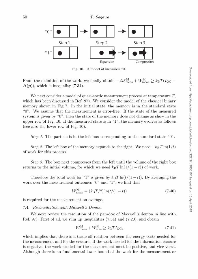
50 T. Sagawa
Fig. 10. A model of measurement.
From the definition of the work, we finally obtain −ΔFMmeas +WM
meas ≥ kBT (IQC −H(p)), which is inequality (7.34).
We next consider a model of quasi-static measurement process at temperature T ,which has been discussed in Ref. 97). We consider the model of the classical binarymemory shown in Fig 7. In the initial state, the memory is in the standard state“0”. We assume that the measurement is error-free. If the state of the measuredsystem is given by “0”, then the state of the memory does not change as show in theupper row of Fig. 10. If the measured state is in “1”, the memory evolves as follows(see also the lower row of Fig. 10).
Step 1. The particle is in the left box corresponding to the standard state “0”.
Step 2. The left box of the memory expands to the right. We need −kBT ln(1/t)of work for this process.
Step 3. The box next compresses from the left until the volume of the right boxreturns to the initial volume, for which we need kBT ln(1/(1 − t)) of work.
Therefore the total work for “1” is given by kBT ln(t/(1− t)). By averaging thework over the measurement outcomes “0” and “1”, we find that
WMmeas = (kBT/2) ln(t/(1 − t)) (7.40)
is required for the measurement on average.
7.4. Reconciliation with Maxwell’s Demon
We next review the resolution of the paradox of Maxwell’s demon in line withRef. 97). First of all, we sum up inequalities (7.34) and (7.20), and obtain
WMmeas +WM
eras ≥ kBTIQC, (7.41)
which implies that there is a trade-off relation between the energy costs needed forthe measurement and for the erasure. If the work needed for the information erasureis negative, the work needed for the measurement must be positive, and vice versa.Although there is no fundamental lower bound of the work for the measurement or
Dow
nloaded from https://academ
ic.oup.com/ptp/article-abstract/127/1/1/1850101 by guest on 15 April 2019
Thermodynamics of Information Processing in Small Systems 51
only for the erasure, there exists a fundamental lower bound on their sum. We notethat we have adopted the commonly used definitions for the measurement and theerasure.9) Under the fixed condition for them, we can still change the ratio of WM
meas
and WMeras by changing the physical structure of the memory, which is described by
FMmeas = −FM
eras.We stress that the lower bound on the total energy cost does not depend on the
Shannon information nor on the free-energy difference, but only on the QC-mutualinformation obtained by the measurement. This fact implies that the origin of thefundamental energy cost is not the randomness of the measurement outcomes whichis described by the Shannon information; but is the correlation between the measuredsystem and the memory which is described by the (QC-)mutual information.
We can illustrate the trade-off relation (7.41) by the model of the binary memorythat has been discussed in the foregoing subsections. By summing up the erasurecost (7.23) and the measurement cost (7.40), we find that the total work is given by
WMmeas +WM
eras = kBT ln 2, (7.42)
with which the equality in (7.41) is achieved. In fact, IQC = H = ln 2 holds in ourmodel.
We now discuss the consistency between the demon and the second law of ther-modynamics. The fundamental upper bound of the work that can be extracted bythe demon has been identified in §6. In particular, if the free-energy difference ΔF S
of the controlled system S is zero, the work that can be extracted by the demon isgiven by
W Sext ≤ kBTIQC. (7.43)
By summing up inequalities (7.41) and (7.43), we obtain
W SMext ≡W S
ext −WMmeas −WM
eras ≤ 0, (7.44)
which implies that the work that can be extracted from the total system of S andM cannot be positive. This is consistent with Kelvin’s principle (5.2) for the cycleof the total system. Therefore, the conventional second law of thermodynamics issatisfied for the total system. We note that the foregoing argument is valid underthe assumption that any element of the POVM corresponds to a single measurementoperator as Ek ≡ M †
kMk. To discuss the cases in which this assumption is notsatisfied is a future challenge.
As discussed in §2, Brillouin argued that, based on a specific model, a positivework is needed for the measurement, which must be larger than the excess workextracted by Maxwell’s demon.12) After that, Bennett proposed a model that canperform measurement without any positive work. Moreover, he argued that, on thebased on a specific model and Landauer’s principle, we always need a positive workto erase the information stored in the memory,13) which has been widely accepted asthe resolution of Maxwell’s demon. Here, we have constructed a model with whichwe do not need any positive work for the information erasure. Moreover, we havederived inequalities (7.41) and (7.44), which enables us to finally reconcile Maxwell’s
Dow
nloaded from https://academ
ic.oup.com/ptp/article-abstract/127/1/1/1850101 by guest on 15 April 2019

52 T. Sagawa
demon with the second law of thermodynamics; what reconciles the demon with thesecond law is the total work of the measurement and erasure, which compensates forthe excess work of kBTIQC that can be extracted by the demon.
We note that kBTIQC of work extracted by the demon can be still useful. Byusing feedback control, we can get the controlled system to obtain the free energyor the work even when there is no direct energy flow between the controller andthe controlled system. We stress that, without feedback control, we need the directenergy input to the system in order to get it to obtain the free energy or the work.
7.5. Second Law of Information Thermodynamics
The conventional second law of thermodynamics cannot be applied to informa-tion processing straightforwardly. On the other hand, our main inequalities (6.17),(7.34), and (7.20) are the generalizations of the second law of thermodynamics forinformation processing processes. In fact, in the limit of H → 0 and IQC → 0, allof inequalities (6.17), (7.34), and (7.20) reduce to the conventional second law ofthermodynamics.
In the inequalities, information content (such as IQC andH) and thermodynamicquantities (such as W and ΔF ) are treated on an equal footing. Therefore, they con-stitute the second law of “information thermodynamics”, which is the generalizationof thermodynamics to information processing processes.
§8. Conclusions
We have reviewed the thermodynamic properties of information processing. Thegeneralized second law of thermodynamics reviewed in this article can be applied tosmall thermodynamic systems that can be precisely controlled by modern experi-mental technologies. The topic of this article is closely related to the fundamentalproblem of Maxwell’s demon, which can be regarded as a feedback controller actingon thermodynamic systems. In the following, we will summarize the main parts ofthis article with several discussions.
In §5, we have reviewed a possible derivation of the second law of thermodynam-ics based on quantum-statistical mechanics. We have formulated the total systemof a thermodynamic system and heat baths obeys a unitary evolution, and the ini-tial states of the heat baths are in the canonical distribution. As a result, we havederived a general form of the second law (5.41), which leads to several expressionsof the second law such as Kelvin’s principle and the Clausius inequality. The reasonwhy we can derive the second law from the unitary dynamics lies in the fact thatwe have set the initial canonical distributions in which the von Neumann entropytakes the maximum values under a given amount of the energy. While this typeof derivation of the second law is a standard method in modern statistical mechan-ics,27),33),51) there would be a room to make the proof physically clearer. In fact,it has been recognized that a thermal equilibrium state of the total system fromthe macroscopic point of view do not necessarily correspond to the canonical (ormicrocanonical) distribution from the microscopic point of view; in fact, even a purestate can behave as a thermal equilibrium state.124)–129) Therefore, it is a future
Dow
nloaded from https://academ
ic.oup.com/ptp/article-abstract/127/1/1/1850101 by guest on 15 April 2019
Thermodynamics of Information Processing in Small Systems 53
challenge to relax the condition of the initial canonical distribution. We note thatsome approaches have been studied in this direction.121),122)
In §§6 and 7, we have reviewed the generalized second law of thermodynamicsto information processing processes by involving quantum information theory to theproof of the second law that is discussed in §5.
In §6, in line with Ref. 87), we have discussed the maximum work (6.17) thatcan be extracted from thermodynamic systems that are subject to feedback control.The maximum work is given by the term of the free energy and the term that isproportional to the QC-mutual information obtained by a measurement. The QC-mutual information, which has been discussed in §4 in detail, represents a kind ofcorrelation between the measured quantum system and the measurement outcomes.The QC-mutual information reduces to the classical mutual information in the casesof classical measurements.
In §7, in line with Ref. 97), we have discussed the minimal works (7.34) and (7.20)that are performed on memories during the measurement and information erasure.The memories can be regarded as the physical implementations of Maxwell’s demon,and therefore these results have identified the minimal work that is needed for thedemon to work. The minimal work for the erasure leads to Landauer’s principle forspecial cases. These results lead to the trade-off relation between the works that areneeded for the measurement and erasure, and the lower bound (7.43) of the sum ofthe works is determined only by the temperature and the QC-mutual information.
The main inequalities in §§6 and 7 imply that the excess work that is extractedfrom Maxwell’s demon is compensated for by the total work that is needed for themeasurement and the erasure. Therefore, these results enable us to reconcile theMaxwell’s demon with the second law of thermodynamics as discussed in Ref. 97),which is different from the previous approaches for the reconciliation. The maininequalities in §§6 and 7 are the generalizations of the second law of thermodynamics,which can be applied to the information processing processes.
We note that the main inequalities in §§6 and 7.3 have been87),97) derived underthe assumption that any element of the POVM corresponds to a single measurementoperator so that Ek = M †
kMk. To relax this assumption is a future challenge.In the generalized second law of thermodynamics, the thermodynamic quanti-
ties, such as the free energy and the work, and the information contents such as theShannon information and the mutual information, are treated on an equal footing.Therefore, our theory reviewed in this article can be regarded as constituting “infor-mation thermodynamics”. Information thermodynamics sheds fundamental lightson the foundations of thermodynamics and statistical mechanics through the para-dox of Maxwell’s demon, and has potential applications to information processing insmall systems such as nanomachines and nanodevices.
Acknowledgements
The author is grateful to Prof. Masahito Ueda, who was the supervisor of theauthor in his Ph.D. course, for fruitful discussions and numerous valuable advices.The main arguments reviewed in this article are based on the author’s researches
Dow
nloaded from https://academ
ic.oup.com/ptp/article-abstract/127/1/1/1850101 by guest on 15 April 2019
54 T. Sagawa
collaborating with Prof. Ueda. The author is grateful to his collaborators Prof.Masaki Sano, Prof. Eiro Muneyuki, and Prof. Shoichi Toyabe for an experimentalwork on Maxwell’s demon. The author is also grateful to many researchers who havegiven him the opportunities of a lot of valuable discussions on this topic in Japan andoverseas. Finally, the author is grateful to Prof. Hisao Hayakawa who has invitedhim to the publication of this review article.
References
1) J. C. Maxwell, Theory of Heat (Appleton, London, 1871).2) S. Carnot, Reflexions sur la pussance motrice du feu et sur les machines propresa
developper atte puissance (Bachelier, 1824).3) L. Tisza and P. M. Quay, Ann. of Phys. 25 (1963), 48.4) E. H. Lieb and J. Yngvason, Phys. Rep. 310 (1999), 1.5) H. B. Callen, Thermodynamics and an Introduction to Thermostatistics, 2nd Ed. (John
Wiley and Sons, New York, 1985).6) H. Tasaki, Thermodynanmics — From a Modern Point of View (Baifu-kan, 2000), in
Japanese.7) S. Sasa, Introduction to Thermodynamics (Kyoritsu, 2000), in Japanese.8) A. Shimizu, Principles of Thermodynamics (University of Tokyo Press, 2007), in
Japanese.9) Maxwell’s demon 2: Entropy, Classical and Quantum Information, Computing, ed. H. S.
Leff and A. F. Rex (Princeton University Press, New Jersey, 2003).10) L. Szilard, Z. Phys. 53 (1929), 840.11) C. Shannon, Bell System Technical Journal 27 (1948), 379; Bell System Technical Journal
27 (1948), 623.12) L. Brillouin, J. Appl. Phys. 22 (1951), 334.13) C. H. Bennett, Int. J. Theor. Phys. 21 (1982), 905.14) R. Landauer, IBM J. Res. Dev. 5 (1961), 183.15) K. Maruyama, F. Nori and V. Vedral, Rev. Mod. Phys. 81 (2009), 1.16) M. Schliwa and G. Woehlke, Nature 422 (2003), 759.17) Y. Shirai et al., Nano Lett. 5 (2005), 2330.18) V. Serreli et al., Nature 445 (2007), 523.19) S. Rahav, J. Horowitz and C. Jarzynski, Phys. Rev. Lett. 101 (2008), 140602.20) E. R. Kay, D. A. Leigh and F. Zerbetto, Angew. Chem. 46 (2007), 72.21) H. Gu et al., Nature 465 (2010), 202.22) K. Sekimoto, Prog. Theor. Phys. Suppl. No. 130 (1998), 17.23) C. Bustamante, J. Liphardt and F. Ritort, Physics Today 58 (2005), 43.24) U. Seifert, Eur. Phys. J. B 64 (2008), 423.25) D. J. Evans, E. G. D. Cohen and G. P. Morriss, Phys. Rev. Lett. 71 (1993), 2401.26) G. Gallavotti and E. G. D. Cohen, Phys. Rev. Lett. 74 (1995), 2694.27) C. Jarzynski, Phys. Rev. Lett. 78 (1997), 2690.28) G. E. Crooks, J. Stat. Phys. 90 (1998), 1481.29) G. E. Crooks, Phys. Rev. E 60 (1999), 2721.30) J. L. Lebowitz and H. Spohn, J. Stat. Phys. 95 (1999), 333.31) C. Maes, J. Stat. Phys. 95 (1999), 367.32) C. Maes, F. Redig and A. V. Moffaert, J. Math. Phys. 41 (2000), 1528.33) C. Jarzynski, J. Stat. Phys. 98 (2000), 77.34) T. Hatano and S.-I. Sasa, Phys. Rev. Lett. 86 (2001), 3463.35) D. J. Evans and D. J. Searles, Adv. Phys. 51 (2002), 1529.36) R. van Zon and E. G. D. Cohen, Phys. Rev. Lett. 91 (2003), 110601.37) C. Jarzynski, J. Stat. Mech. (2004), P09005.38) C. Jarzynski and D. K. Wojcik, Phys. Rev. Lett. 92 (2004), 230602.39) D. Andrieux and P. Gaspard, J. Chem. Phys. 121 (2004), 6167.40) T. Harada and S.-I. Sasa, Phys. Rev. Lett. 95 (2005), 130602.41) U. Seifert, Phys. Rev. Lett. 95 (2005), 040602.42) T. Ohkuma and T. Ohta J. Stat. Mech. (2007), P10010.
Dow
nloaded from https://academ
ic.oup.com/ptp/article-abstract/127/1/1/1850101 by guest on 15 April 2019
Thermodynamics of Information Processing in Small Systems 55
43) R. Kawai, J. M. R. Parrondo and C. Van den Broeck, Phys. Rev. Lett. 98 (2007), 080602.44) A. Gomez-Marin, J. M. R. Parrondo and C. Van den Broeck, Phys. Rev. E 78 (2008),
011107.45) T. S. Komatsu and N. Nakagawa, Phys. Rev. Lett. 100 (2008), 030601.46) T. S. Komatsu, N. Nakagawa, S.-I. Sasa and H. Tasaki, Phys. Rev. Lett. 100 (2008),
230602.47) H.-H. Hasegawa, J. Ishikawa, K. Takara and D. J. Driebe, Phys. Lett. A 374 (2010),
1001.48) M. Esposito and C. Van den Broeck, Phys. Rev. Lett. 104 (2010), 090601.49) S. Vaikuntanathan and C. Jarzynski, Europhys. Lett. 87 (2009), 60005.50) J. Kurchan, cond-mat/0007360.51) H. Tasaki, cond-mat/0009244.52) M. Esposito and S. Mukamel, Phys. Rev. E 73 (2006), 046129.53) K. Saito and A. Dhar, Phys. Rev. Lett. 99 (2007), 180601.54) Y. Utsumi and K. Saito, Phys. Rev. B 79 (2009), 235311.55) M. Campisi, P. Talkner and P. Hanggi, Phys. Rev. Lett. 102 (2009), 210401.56) J. Ren, P. Hanggi and B. Li, Phys. Rev. Lett. 104 (2010), 170601.57) A. Shimizu and T. Yuge, J. Phys. Soc. Jpn. 79 (2010), 013002.58) A. Shimizu, J. Phys. Soc. Jpn. 79 (2010), 113001.59) G. M. Wang et al., Phys. Rev. Lett. 89 (2002), 050601.60) J. Liphardt et al., Science 296 (2002), 1832.61) E. H. Trepagnier et al., Proc. Natl. Acad. Sci. USA 101 (2004), 15038.62) D. M. Carberry et al., Phys. Rev. Lett. 92 (2004), 140601.63) D. Collin et al., Nature 437 (2005), 231.64) F. Douarche et al., Phys. Rev. Lett. 97 (2006), 140603.65) D. Andrieux et al., Phys. Rev. Lett. 98 (2007), 150601.66) S. Toyabe et al., Phys. Rev. E 75 (2007), 011122.67) S. Toyabe et al., Phys. Rev. Lett. 104 (2010), 198103.68) K. Hayashi et al., Phys. Rev. Lett. 104 (2010), 218103.69) S. Nakamura et al., Phys. Rev. Lett. 104 (2010), 080602.70) J. von Neumann, Mathematische Grundlagen der Quantumechanik (Springer, Berlin,
1932) [Eng. trans. R. T. Beyer, Mathematical Foundations of Quantum Mechanics (Prin-ston University Press, Princeton, 1955)].
71) E. B. Davies and J. T. Lewis, Commun. Math. Phys. 17 (1970), 239.72) K. Kraus, Ann. of Phys. 64 (1971), 311.73) M. Ozawa, J. Math. Phys. 25 (1984), 79.74) M. A. Nielsen and I. L. Chuang, Quantum Computation and Quantum Information (Cam-
bridge University Press, Cambridge, 2000).75) H. P. Breuer and F. Petruccione, The theory of open quantum systems (Oxford University
Press, Oxford, 2002).76) K. Koshino and A. Shimizu, Phys. Rep. 412 (2005), 191.77) H. M. Wiseman and G. J. Milburn, Quantum Measurement and Control (Cambridge
University Press, Cambridge, UK, 2010).78) T. M. Cover and J. A. Thomas, Elements of Information Theory (John Wiley and Sons,
New York, 1991).79) S. Lloyd and W. H. Zurek, J. Stat. Phys. 62 (1991), 819.80) H. Touchette and S. Lloyd, Phys. Rev. Lett. 84 (2000), 1156.81) W. H. Zurek, quant-ph/0301076.82) M. O. Scully et al., Science 299 (2003), 862.83) T. D. Kieu, Phys. Rev. Lett. 93 (2004), 140403.84) A. E. Allahverdyan et al., J. Mod. Optics 51(2004), 2703.85) H. T. Quan et al., Phys. Rev. Lett. 97 (2006), 180402.86) M. A. Nielsen, C. M. Caves, B. Schumacher and H. Barnum, Proc. R. Soc. London A,
454 (1998), 277.87) T. Sagawa and M. Ueda, Phys. Rev. Lett. 100 (2008), 080403.88) K. Jacobs, Phys. Rev. A 80 (2009), 012322.89) K. Shizume, Phys. Rev. E 52 (1995), 3495.90) M. O. Magnasco, Europhys. Lett. 33 (1996), 583.
Dow
nloaded from https://academ
ic.oup.com/ptp/article-abstract/127/1/1/1850101 by guest on 15 April 2019
56 T. Sagawa
91) H. Matsueda, E. Goto and K-F. Loe, RIMS Kokyuroku 1013 (1997), 187.92) B. Piechocinska, Phys. Rev. A 61 (2000), 062314.93) M. M. Barkeshli, cond-mat/0504323.94) O. J. E. Maroney, Phys. Rev. E 79 (2009), 031105.95) C. Horhammer and H. Buttner, J. Stat. Phys. 133 (2008), 1161.96) R. Dillenschneider and E. Lutz, Phys. Rev. Lett. 102 (2009), 210601.97) T. Sagawa and M. Ueda, Phys. Rev. Lett. 102 (2009), 250602; [Errata; 106 (2011),
189901].98) F. J. Cao, L. Dinis and J. M. R. Parrondo, Phys. Rev. Lett. 93 (2004), 040603.99) K. H. Kim and H. Qian, Phys. Rev. E 75 (2007), 022102.
100) B. J. Lopez et al., Phys. Rev. Lett. 101 (2008), 220601.101) F. J. Cao and M. Feito, Phys. Rev. E 79 (2009), 041118.102) M. Feito, J. P. Baltanas and F. J. Cao, Phys. Rev. E 80 (2009), 031128.103) M. Bonaldi et al., Phys. Rev. Lett. 103 (2009), 010601.104) H. Suzuki and Y. Fujitani, J. Phys. Soc. Jpn. 78 (2009), 074007.105) T. Sagawa and M. Ueda, Phys. Rev. Lett. 104 (2010), 090602.106) S. W. Kim, T. Sagawa, S. De Liberato and M. Ueda, Phys. Rev. Lett. 106 (2011), 070401.107) Y. Fujitani and H. Suzuki, J. Phys. Soc. Jpn. 79 (2010), 104003.108) T. Brandes, Phys. Rev. Lett. 105 (2010), 060602.109) M. Ponmurugan, Phys. Rev. E 82 (2010), 031129.110) J. M. Horowitz and S. Vaikuntanathan, Phys. Rev. E 82 (2010), 061120.111) Y. Morikuni and H. Tasaki, J. Stat. Phys. 143 (2011), 1.112) S. Ito and M. Sano, Phys. Rev. E 84 (2011), 021123.113) J. M. Horowitz and J. M. R. Parrondo, Europhys Lett. 95 (2011), 10005.114) D. Abreu and U. Seifert, Europhys Lett. 94 (2011), 10001.115) S. Vaikuntanathan and C. Jarzynski, Phys. Rev. E 83 (2011), 061120.116) S. Toyabe, T. Sagawa, M. Ueda, E. Muneyuki and M. Sano, Nature Physics 6 (2010),
988.117) J. C. Doyle, B. A. Francis and A. R. Tannenbaum, Feedback Control Theory (Macmillan,
New York, 1992).118) K. J. Astrom and R. M. Murray, Feedback Systems: An Introduction for Scientists and
Engineers (Princeton University Press, 2008).119) H. J. Groenewold, Int. J. Theor. Phys. 4 (1971), 327.120) M. Ozawa, J. Math. Phys. 27 (1986), 759.121) A. Lenard, J. Stat. Phys. 19 (1978), 575.122) H. Tasaki, cond-mat/0009206.123) J. M. R. Parrondo and B. J. De Cisneros, Appl. Phys. A 75 (2002), 179.124) J. von Neumann, Z. Phys. 57 (1929), 30 [Eng. Trans. in arXiv:1003.2133].125) H. Tasaki, Phys. Rev. Lett. 80 (1998), 1373.126) A. Sugita, RIMS Kokyuroku, 1507 (2006), 147, in Japanese.127) S. Goldstein, J. L. Lebowitz, R. Tumulka and N. Zanghi, Phys. Rev. Lett. 96 (2006),
050403.128) S. Popescu, A. J. Short and A. Winter, Nature Physics 2 (2006), 754.129) P. Reimann, Phys. Rev. Lett. 99 (2007), 160404.
Dow
nloaded from https://academ
ic.oup.com/ptp/article-abstract/127/1/1/1850101 by guest on 15 April 2019