Realistically Coupled Neural Mass Models Can Generate EEG Rhythms

8/6/2019 Realistically Coupled Neural Mass Models Can Generate EEG Rhythms

http://slidepdf.com/reader/full/realistically-coupled-neural-mass-models-can-generate-eeg-rhythms 1/31

LETTER Communicated by Olivier Faugeras

Realistically Coupled Neural Mass Models Can Generate EEGRhythms

Roberto C. [email protected]

Nelson J. [email protected]

Yasser Iturria-Medina

[email protected] Neuroscience Center, Brain Dynamics Department, Havana, Cuba

Felix Carbonell [email protected]

Juan C. Jimenez [email protected]

Instituto de Cibern´ etica Matem´ atica y F´ ısica, Departamento de Sistemas Adaptativos,

Havana, Cuba

We study the generation of EEG rhythms by means of realistically cou-pled neural mass models. Previous neural mass models were used tomodel cortical voxels and the thalamus. Interactions between voxels ofthe same and other cortical areas and with the thalamus were taken intoaccount. Voxels within the same cortical area were coupled (short-rangeconnections) with both excitatory and inhibitory connections, while cou-pling between areas (long-range connections) was considered to be ex-citatory only. Short-range connection strengths were modeled by usinga connectivity function depending on the distance between voxels. Cou-

pling strength parameters between areas were defined from empiricalanatomical data employing the information obtained from probabilisticpaths, which were tracked by water diffusion imaging techniques andused to quantify white matter tracts in the brain. Each cortical voxel wasthen described by a set of 16 random differential equations, while thethalamus was described by a set of 12 random differential equations.Thus, for analyzing the neuronal dynamics emerging from the interac-tion of several areas, a large system of differential equations needs tobe solved. The sparseness of the estimated anatomical connectivity ma-trix reduces the number of connection parameters substantially, makingthe solution of this system faster. Simulations of human brain rhythmswere carried out in order to test the model. Physiologically plausible re-sults were obtained based on this anatomically constrained neural massmodel.

Neural Computation 19, 478–512 (2007) C 2007 Massachusetts Institute of Technology



Realistic Neural Mass Models 479

1 Introduction

We aim at describing a generative model of EEG rhythms based on anatomi-cally constrained coupling of neural mass models. Although the biophysicalmechanisms underlying oscillatory activity in neurons are well studied, theorigin and function of global characteristics (such as EEG rhythms) of largepopulations of neurons are still unknown. In this context, computationalmodels have proven capable of providing insight into this problem. Twomodeling approaches have been used to study the behavior of neuronalpopulations. One approach is based on the study of large computationalneuronal networks in which each cell is realistically represented by mul-tiple compartments for the soma, axon, and dendrites, and each synaptic

connection is modeled explicitly (Traub & Miles, 1991). A disadvantage ofsuch realistic modeling is that it requires high computational power. Forthis reason, simplified versions of such models in which only one compart-ment model was taken into account have been used (Wang, Golomb, &Rinzel, 1995; Rinzel, Terman, Wang, & Ermentrout, 1998). However, evenin this case, the use of such detailed models makes it difficult to determinethe influence of each model parameter on the generated average networkcharacteristics. The second approach is based on the use of neural massmodels (NMM). In contrast to neuronal networks, NMMs describe the dy-

namics of cortical columns and brain areas by using only a few parameters, but without much detail. In this approach, spatially averaged magnitudesare assumed to characterize the collective behavior of populations of neu-rons of a given type instead of modeling single cells and their interac-tions in a detailed network (Wilson & Cowan, 1972; Lopes da Silva, Hoeks,Smits, & Zetterberg, 1974; Zetterberg, Kristiansson, & Mossberg, 1978; vanRotterdam, Lopes da Silva, van den Ende, Viergever, & Hermans, 1982; Jansen & Rit, 1995; Valdes, Jimenez, Riera, Biscay, & Ozaki, 1999; Wendling,Bellanger, Bartolomei, & Chauvel, 2000; David & Friston, 2003).

Despite their simplicity, NMMs have been very helpful in the study

of EEG rhythms. For example, in order to study the origin of the alpharhythm, Lopes da Silva et al. (1974) developed an NMM comprising twointeracting populations of neurons, the thalamocortical relay cells and theinhibitory interneurons, which were interconnected by a negative feedbackloop. Later, this model was extended to include both positive and negativefeedback loops (Zetterberg et al., 1978; Jansen, Zouridakis, & Brandt, 1993).In Jansen and Rit (1995), alpha and beta activities were replicated by usingtwo coupled neural mass models representing cortical areas with delaysin the interconnections between them. Wendling et al. (2000) investigated

the generation of epileptic spikes by extending Jansen’s model to multiplecoupled areas but explored the dynamics of only three areas for differentvalues of the connectivity constants. David and Friston (2003) consideredthat a cortical area comprises several noninteracting neuronal populationsthat were in turn described by Jansen’s models. This model allowed them



480 R. Sotero et al.

to reproduce the whole spectrum of EEG signals by changing the coupling between two of these areas, thus showing the importance of parametersrelated to the coupling between different brain regions for the resultingdynamics.

Due to the lack of information about actual connectivity patterns, previ-ous approaches have been devoted to the study of the temporal evolutionof neuronal populations rather than their spatial dynamics. However, thedevelopment of techniques such as diffusion weighted magnetic resonanceimaging (DWMRI) in the past 20 years makes noninvasive study of theanatomical brain circuitry of the living human brain possible. This has putat our disposal extremely valuable information and gives us a unique op-portunity to formulate models that take into account a more realistic view

of the central nervous system.In this article, we extend Jansen’s model to characterize the dynamics of

a cortical voxel. Building on this, our goal is to study the rhythms obtainedwhen coupling several areas comprising large numbers of interconnectedvoxels. In this approach, voxels of the same cortical area are assumed to be coupled with excitatory and inhibitory connections (short-range con-nections), while connections between areas (long-range connections) areassumed to be excitatory only. This is an extension of the model of Davidand Friston (2003) because interactions between voxels within the same area

are taken into account. Additionally, we introduce anatomical constraintson coupling strength parameters (CSP) between different brain regions.This is accomplished by using CSPs estimated from human DWMRI data(Iturria-Medina, Canales-Rodrıguez, Melie-Garcia, & Valdes-Hernandez,2005). The thalamus is also modeled using a single NMM, mutually cou-pled with the cortical areas. We show that this anatomically constrainedNMM can reproduce the EEG rhythms recorded at the scalp, another stepin the validation of NMMs as a valuable tool for describing the activity oflarge populations of neurons.

The letter is organized as follows. In section 2, the NMMs used for a

cortical voxel and the thalamus are formulated. Section 3 is devoted tothe modeling of short-range and long-range interactions. The integratedthalamocorticalmodel is formulated in section 4. In section 5 the observationmodel that links the activity in a cortical voxel with the recorded EEG on thescalp surface is presented. Section 6 describes the numerical method usedfor integrating the huge system of random differential equations obtained.Finally, sections 7 and 8 are devoted to a description of the simulations aswell as a discussion of the results.

2 Models for a Cortical Voxel and the Thalamus

In this work we model the neuronal activity in a cortical voxel by extend-ing previous neural mass models that have been used to describe neu-ral dynamics at smaller spatial scales. In particular, Jansen and Rit (1995)




A

B

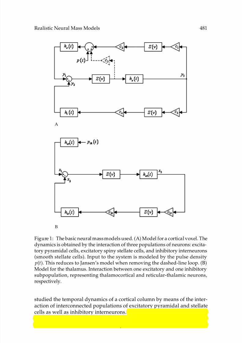
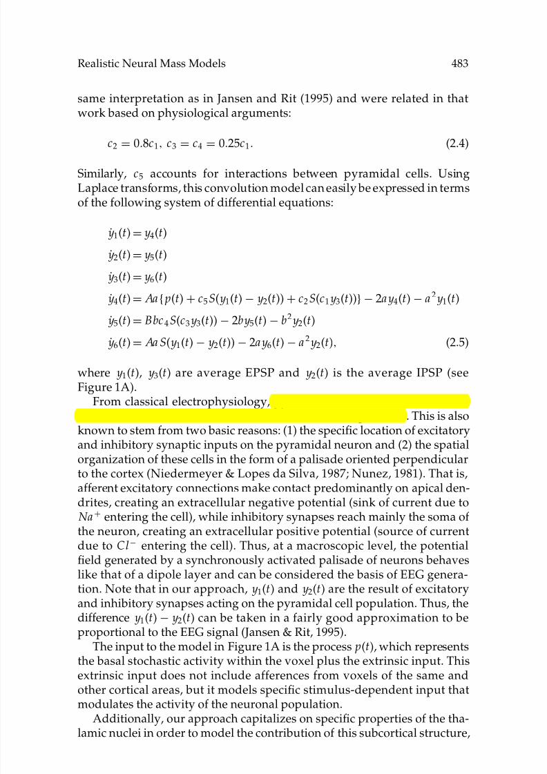
Figure 1: The basic neural mass models used. (A) Model for a cortical voxel. Thedynamics is obtained by the interaction of three populations of neurons: excita-tory pyramidal cells, excitatory spiny stellate cells, and inhibitory interneurons(smooth stellate cells). Input to the system is modeled by the pulse density p(t). This reduces to Jansen’s model when removing the dashed-line loop. (B)Model for the thalamus. Interaction between one excitatory and one inhibitorysubpopulation, representing thalamocortical and reticular-thalamic neurons,respectively.

studied the temporal dynamics of a cortical column by means of the inter-action of interconnected populations of excitatory pyramidal and stellatecells as well as inhibitory interneurons. This model (see Figure 1A, exceptfor the dashed-line loop) capitalizes on the basic circuitry of the corticalcolumn (Mountcastle, 1978, 1997). Pyramidal cells receive feedback from




excitatory and inhibitory interneurons, which receive only excitatoryinput from pyramidal cells. Nevertheless, at the spatial scale of voxels,this simplified circuitry is no longer valid, but more complicated interac-tions need to be considered. While a cortical column has a diameter of 150 to300µm, the length of a voxel usually ranges from 1 to 3 mm, comprising sev-eral interconnected columns. At this spatial scale, pyramidal-to-pyramidalconnections become increasingly important, accounting for the majority ofintracortical fibers (Braitenberg & Schuz, 1998). In our approach, Jansen’smodel is extended to include this kind of connection by adding a self-excitatory loop for the pyramidal population (see Figure 1B). Zetterberget al. (1978) had already used a generic model of this kind for describingthe temporal dynamics of a neuronal mass consisting of two excitatory

and one inhibitory population. Although they were able to produce signalsresembling EEG background activity, their model had no specific neuralsubstrate.

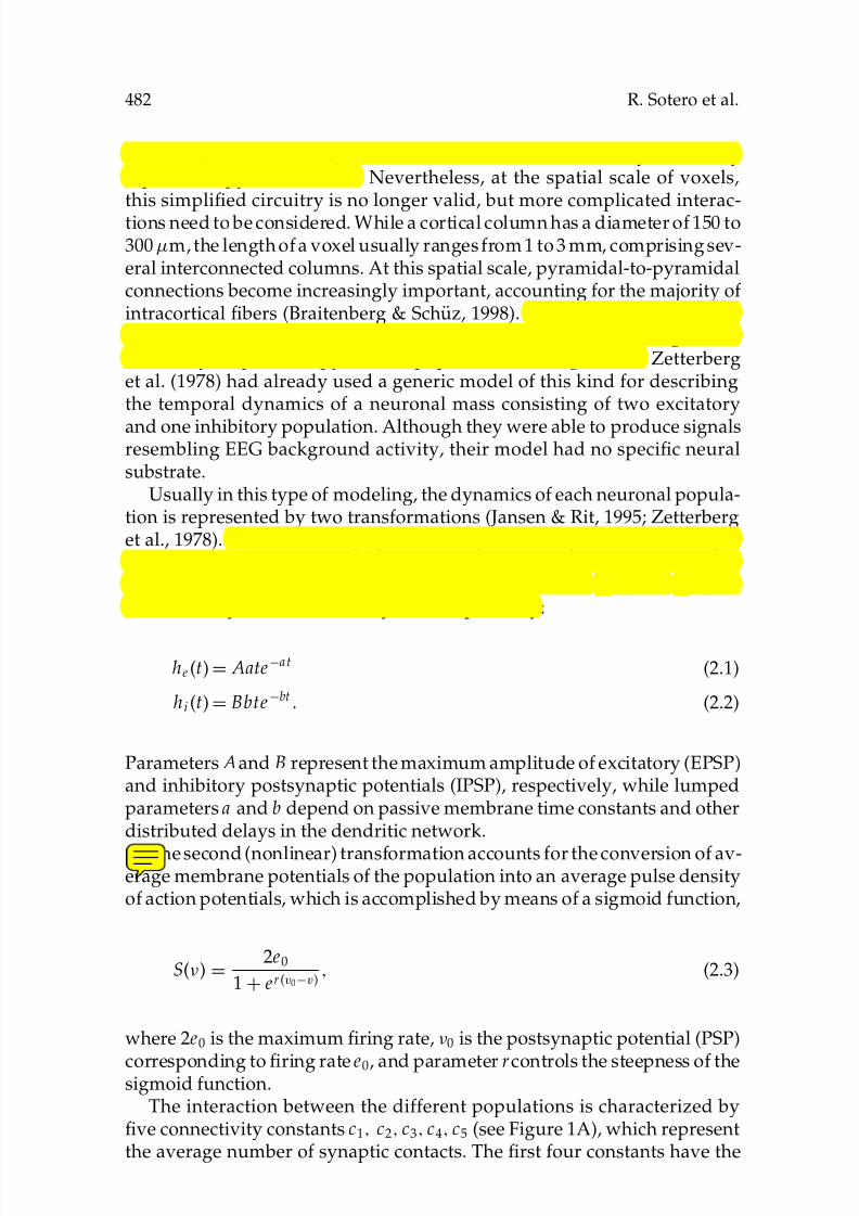
Usually in this type of modeling, the dynamics of each neuronal popula-tion is represented by two transformations (Jansen & Rit, 1995; Zetterberget al., 1978). First, the average pulse density of action potentials entering apopulation is converted into an average postsynaptic membrane potential by means of linear convolutions with impulse responses he (t) and hi (t) forthe excitatory and the inhibitory case, respectively:

he (t)= Aate−a t (2.1)

hi (t)= Bbte−bt . (2.2)

Parameters Aand B represent the maximum amplitude of excitatory (EPSP)and inhibitory postsynaptic potentials (IPSP), respectively, while lumpedparameters a and b depend on passive membrane time constants and otherdistributed delays in the dendritic network.

The second (nonlinear) transformation accounts for the conversion of av-erage membrane potentials of the population into an average pulse densityof action potentials, which is accomplished by means of a sigmoid function,

S(ν) =2e0

1+ er (v0−v), (2.3)

where 2e0 is the maximum firing rate, ν0 is the postsynaptic potential (PSP)

corresponding to firing rate e0, and parameter rcontrols the steepness of thesigmoid function.

The interaction between the different populations is characterized byfive connectivity constants c1, c2, c3, c4, c5 (see Figure 1A), which representthe average number of synaptic contacts. The first four constants have the




same interpretation as in Jansen and Rit (1995) and were related in thatwork based on physiological arguments:

c2 = 0.8c1, c3 = c4 = 0.25c1. (2.4)

Similarly, c5 accounts for interactions between pyramidal cells. UsingLaplace transforms, this convolution model can easily be expressed in termsof the following system of differential equations:

˙ y1(t)= y4(t)

˙ y2(t)= y5(t)

˙ y3(t)= y6(t)

˙ y4(t)= Aa{ p(t) + c5 S( y1(t) − y2(t))+ c2 S(c1 y3(t))} − 2a y4(t) − a 2 y1(t)

˙ y5(t)= Bbc 4 S(c3 y3(t)) − 2by5(t) − b2 y2(t)

˙ y6(t)= Aa S( y1(t) − y2(t)) − 2a y6(t) − a 2 y2(t), (2.5)

where y1(t), y3(t) are average EPSP and y2(t) is the average IPSP (seeFigure 1A).

From classical electrophysiology, pyramidal cells are considered to bethe main contributors to the measured EEG at the scalp surface. This is alsoknown to stem from two basic reasons: (1) the specific location of excitatoryand inhibitory synaptic inputs on the pyramidal neuron and (2) the spatialorganization of these cells in the form of a palisade oriented perpendicularto the cortex (Niedermeyer & Lopes da Silva, 1987; Nunez, 1981). That is,afferent excitatory connections make contact predominantly on apical den-drites, creating an extracellular negative potential (sink of current due toNa+ entering the cell), while inhibitory synapses reach mainly the soma ofthe neuron, creating an extracellular positive potential (source of current

due to Cl− entering the cell). Thus, at a macroscopic level, the potentialfield generated by a synchronously activated palisade of neurons behaveslike that of a dipole layer and can be considered the basis of EEG genera-tion. Note that in our approach, y1(t) and y2(t) are the result of excitatoryand inhibitory synapses acting on the pyramidal cell population. Thus, thedifference y1(t) − y2(t) can be taken in a fairly good approximation to beproportional to the EEG signal (Jansen & Rit, 1995).

The input to the model in Figure 1A is the process p(t), which representsthe basal stochastic activity within the voxel plus the extrinsic input. This

extrinsic input does not include afferences from voxels of the same andother cortical areas, but it models specific stimulus-dependent input thatmodulates the activity of the neuronal population.

Additionally, our approach capitalizes on specific properties of the tha-lamic nuclei in order to model the contribution of this subcortical structure,




which is the main relay station of the sensory input on its way to the cor-tex. That is, the thalamus comprises two major populations of neurons:thalamocortical (TC) excitatory relay neurons and thalamic inhibitory retic-ular (RE) neurons. Only the axons of TC neurons project to the cortex,while RE neurons form an inhibitory network that surrounds the thalamusand project inhibitory connections to TC neurons exclusively (Destexhe &Sejnowski, 2001). This circuitry allowed us to formulate the mass modelshown in Figure 1B, which Lopes da Silva et al. (1974) used for simulatingthe alpha rhythm. Note that the model is used to describe the dynamicsof the thalamus as a whole, without taking into account any subdivisioninto voxels. The motivation for this was the physical separation of the twotypes of neuronal populations that form the thalamus. On the other hand,

the absence of any preferential orientation of the neurons in the thalamus,together with the depth of this structure, has led to the idea that it doesnot generate any measurable voltage at the scalp surface. Thus, in our ap-proach, no direct thalamic contribution to the EEG is considered. A moresophisticated model of the thalamic activity could be used to elucidate itsactual contribution to the EEG generation, but that would entail a detailedknowledge of its microscopic cytoarchitectonic organization, which we lackat the moment.

3 Short-Range versus Long-Range Interactions

If we want to model the dynamics of macroscopic cortical areas, we haveto augment the model described to account for the specific neuronal inter-actions in the brain. In the cytoarchitectonic organization of the cerebralcortex, two types of connections can be distinguished: short-range andlong-range connections (SRC and LRC, respectively). SRCs are made bycortical neurons with local branches that can reach a maximum of about10 mm (Braitenberg, 1978; Abeles, 1991; Jirsa & Haken, 1997) corresponding

to the length of the longest horizontal axon collaterals plus the length ofthe longest dendrites. LRCs are mainly formed by axons of pyramidal cellsthat cross the white matter and connect cortical regions that can be up to100 mm apart (Abeles, 1991; Jirsa & Haken, 1997).

Several differences between these two systems can be established, notonly in their characteristic lengths but also in their specificity and function(Abeles, 1991; Braitenberg & Schuz, 1998). While SRCs can be described instatistical terms, with an effective connection strength that diminishes ex-ponentially with the distance between neuronal populations, LRCs do not

show such a regular and smooth pattern but have a high degree of speci-ficity. Additionally, LRCs terminate preferentially on the apical dendrites ofpyramidal cells, while local collaterals terminate more on basal dendrites.In the following sections, we describe how this differentiation of corticalinteractions is incorporated into our model.




3.1 Within-Area Interactions. First, SRCs that mediate neuronal inter-actions within a cortical area will be described. A diagram of the proposedaugmented model for a given voxel is shown in Figure 2A. We assumethat voxels of the same area are coupled by means of both excitatory andinhibitory connections, where the pyramidal cell population is the targetof all the input to the system. Excitatory input comes from pyramidal andspiny stellate cell populations with coupling strengths described by con-nectivity functions that depend on the distance between voxels |xm − x j |(Jirsa & Haken, 1996, 1997):

kmje1 =

1

2σ e1e−|xm−x j |

σ e1 (3.1)

kmje2 =

1

2σ e2e−|xm−x j |

σ e2 . (3.2)

In equations 3.1 and 3.2, kmje1 and k

mje2 are the strengths of the connections that

pyramidal cells and excitatory interneurons of voxel m make on pyramidalcells of voxel j , respectively. Delays in these connections can be modeled bylinear transformations similar to equation 2.1, as in Jansen and Rit (1995).We use hd2(t) and hd3(t), respectively:

hd2(t)= Aad2te−ad2t (3.3)

hd3(t)= Aad3te−ad3t. (3.4)

Similar equations are formulated for within-area inhibitory connections,

which are considered by means of the connection strength kmji that in-

hibitory interneurons (smooth stellate cells) of voxel m exert on pyramidalcells of voxel j , that is,

kmji = 12σ ie−

|xm−x j |

σ i (3.5)

hd4(t)= Bbd4te−bd4t. (3.6)

3.2 Between-Area Interactions. Interactions between distant corticalareas are determined by LRCs, which in our approach are mediated bypyramidal-to-pyramidal cell connections. There is no clarity about the rulesgoverning the system of LRCs (Braitenberg & Schuz, 1998). Nevertheless,the emergence of new imaging techniques like diffusion weighted magnetic

resonance imaging (DWMRI) in the past few years has opened a windowto the study of this type of connection in the living human brain. DWMRIis based on the fact that trajectories followed by water molecules duringdiffusion processes reflect the microscopic environment of brain tissues.Then nervous fibers can be characterized by tracing probabilistic paths




Figure 2: The thalamocortical model. (A) Input-output relationship for the neu-ral mass model of a cortical voxel. A cortical voxel receives excitatory afferencesfrom pyramidal cells and excitatory stellate cells of voxels of the same area, frompyramidal cells of other cortical areas, and from TC relay neurons. Inhibitoryafferences are received from inhibitory interneurons of voxels of the same area.The pulse density p(t) accounts for the basal stochastic activity within the voxel.

(B) Input-output relationship for the neural mass model of the thalamus. TCrelay neurons send axonal projections to the cortex, where they make synapseson the three populations of neurons considered. TC cells receive backward con-nections from cortical pyramidal neurons. The pulse density pth (t) accounts forthe background stochastic activity within the thalamus plus stimulus relatedinputs.




that represent the preferred direction of water diffusion along the nervousfibers in each voxel. Finally, measures of anatomical connectivity reflectingthe interrelation between voxels and areas can be defined and calculated based on these paths. In this article, the LRC strength K i,n between twoareas i and n will be estimated from actual DWMRI data.

Most work in the field of DWMRI has defined measures of between-voxel rather than between-areas anatomical connectivity. For example, forcharacterizing the probability of connection of a point R with a point P , onecan use the number of probabilistic paths leaving P and entering R divided by the number of probabilistic paths generated in P (Behrens et al., 2003;Hagmann et al., 2003; Parker, Wheeler-Kingshott, & Barker, 2002; Koch,Norris, & Hund-Georgiadis, 2002). In Tuch (2002) the probability of connec-

tion between two points is estimated as the probability of the most prob-able paths joining both points, while in Parker et al. (2002) and Tournier,Calamate, Gadian, & Connelly, (2003), it is taken as the probability of thepath that minimizes a cost function depending on diffusion data. However,diffusion data generally show high isotropy within the gray matter, givingpoor information about the distribution of nerve fibers. Consequently, inmost cases, it is not convenient to trace probabilistic paths within gray mat-ter areas. Another approach for studying connectivity in the brain is to useonly the points at the boundaries of gray matter regions for characterizing

connection strengths between zones and not between the individual voxelscomprising them. In this line of work, Iturria-Medina, Canales-Rodrıguezet al. (2005) and Iturria-Medina, Valdes-Hernandez et al. (2005) proposed amodel for obtaining anatomical connection strengths (ACS) between brainzones. In their method, the ACS between two regions, A and B (C A↔B ),was defined as being proportional to the cross-section area of the totalcylindrical-shaped volume of the nervous fibers shared by these regions.ACS was then calculated as the area occupied by the connector volume overthe surfaces of the connected zones,

C A↔B = AT ( A,B) + BT ( A,B), (3.7)

where AT ( A,B) and BT ( A,B) represent the area defined by fibers (both afferentand efferent), joining A with B over the surface of A and B, respectively.These areas were evaluated from a DWMRI data set by measuring thenumber of target voxels on each surface of the generated probabilistic pathsthat simulate fiber trajectories under the assumption that those paths arecontained inside the connector volume.

Notice that methods for reconstructing fiber paths using DWMRI datacannot distinguish between excitatory and inhibitory connections. How-ever, in the proposed model, LRCs are considered to be excitatory only.This assumption is consistent with physiological and anatomical studies,demonstrating, that pyramidal cells of layer III are the main source of the




feedforward projections to other cortical areas (Gilbert & Wiesel, 1979, 1983;Martin & Whitteridge, 1984; McGuire, Gilbert, Rivlin, & Wiesel, 1991; Dou-glas & Martin, 2004). Thus, information obtained from DWMRI data can beused as a measure of the CSP (K i,n) between any two given areas i and n.

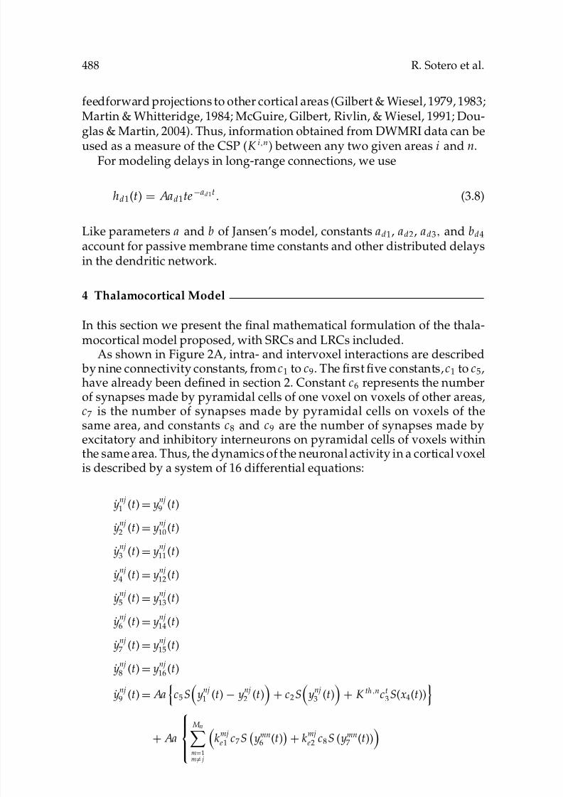
For modeling delays in long-range connections, we use

hd1(t) = Aad1te−ad1t. (3.8)

Like parameters a and b of Jansen’s model, constants ad1, ad2, ad3, and bd4

account for passive membrane time constants and other distributed delaysin the dendritic network.

4 Thalamocortical Model

In this section we present the final mathematical formulation of the thala-mocortical model proposed, with SRCs and LRCs included.

As shown in Figure 2A, intra- and intervoxel interactions are described by nine connectivity constants, from c1 to c9. The first five constants, c1 to c5,have already been defined in section 2. Constant c6 represents the numberof synapses made by pyramidal cells of one voxel on voxels of other areas,c

7is the number of synapses made by pyramidal cells on voxels of the

same area, and constants c8 and c9 are the number of synapses made byexcitatory and inhibitory interneurons on pyramidal cells of voxels withinthe same area. Thus, the dynamics of the neuronal activity in a cortical voxelis described by a system of 16 differential equations:

˙ ynj1 (t)= ynj

9 (t)

˙ ynj2 (t)= ynj

10 (t)

˙ ynj

3(t)= y

nj

11(t)

˙ ynj4 (t)= ynj

12 (t)

˙ ynj5 (t)= ynj

13 (t)

˙ ynj6 (t)= ynj

14 (t)

˙ ynj7 (t)= ynj

15 (t)

˙ ynj8 (t)= ynj

16 (t)

˙ ynj

9 (t)= Aa

c5 S

ynj

1 (t) − ynj

2 (t)+ c2 S

y

nj

3 (t)+ K

th,n

ct

3 S(x4(t))

+ Aa

Mnm=1m= j

kmj

e1 c7 S ymn

6 (t)+ kmj

e2 c8 S ( ymn7 (t))




+N

i=1i=n

K i,n

Mi

m=1

c6 S yim5 (t)

− 2a ynj9 (t) − a 2 ynj

1 (t) + Aa pnj (t)

˙ ynj10 (t)= Bb

c4 S

y

nj4 (t)

+

Mnm=1m= j

kmji c9 S

ynm

8 (t)− 2by

nj10 (t) − b2 y

nj2 (t)

˙ ynj11 (t)= Aa

c1 S

ynj

1 (t)− ynj2 (t)

+ K th,nct

4 S(x5(t))− 2aynj

11 (t) − a 2 ynj3 (t)

˙ ynj12 (t)= Aa

c3 S

ynj

1 (t) − ynj2 (t)

+ K th,nct

5 S (x6(t))− 2a ynj

12 (t) − a 2 ynj4 (t)

˙ ynj13 (t)= Aad1 S

ynj1 (t) − ynj2 (t)− 2ad1 ynj13 (t) − a 2d1 ynj5 (t)

˙ ynj14 (t)= Aa21 S

ynj

1 (t)− ynj2 (t)

− 2ad2 y

nj14 (t) − a 2

d2 ynj6 (t)

˙ ynj15 (t)= Aad3 S

ynj

3 (t)− 2ad3 y

nj15 (t)− a 2

d3 ynj7 (t)

˙ ynj16 (t)= Bbd4 S

ynj

4 (t)− 2bd4 y

nj16 (t) − b2

d4 ynj8 (t), (4.1)

where the superscript nj refers to the voxel j in the area n. The systemhas extrinsic inputs given by connections from other cortical voxels and thethalamus as well as an intrinsic input p(t) that represents baseline stochastic

activity within the voxel. The output is taken as ynj1 (t) − y

nj2 (t), which from

section 2 can be considered proportional to the generated EEG signal. Notethat close voxels separated by the boundary of two neighboring regions areconsidered to be coupled through LRC solely, even if they are close enoughfor the SRC to be important. This simplification can easily be avoided by

adding relevant terms to the equations for ˙ ynj9 and ˙ y

nj10 in equation 4.1.

Nevertheless, in the calculations shown here, all anatomical areas were

chosen large enough and the activation regions within each area locateddistant enough such that boundary effects could be neglected. This allowedus to keep equations simple for the sake of a better understanding of themodel.

In the case of the thalamus, the main output of the system is mediated by TC cells, which are assumed to send axonal projections to the threepopulations of neurons in the cortex: pyramidal, spiny stellate, and smoothstellate cells (see Figure 2). On the contrary, only pyramidal cells project back to the thalamus and make synapses on TC neurons. This model is

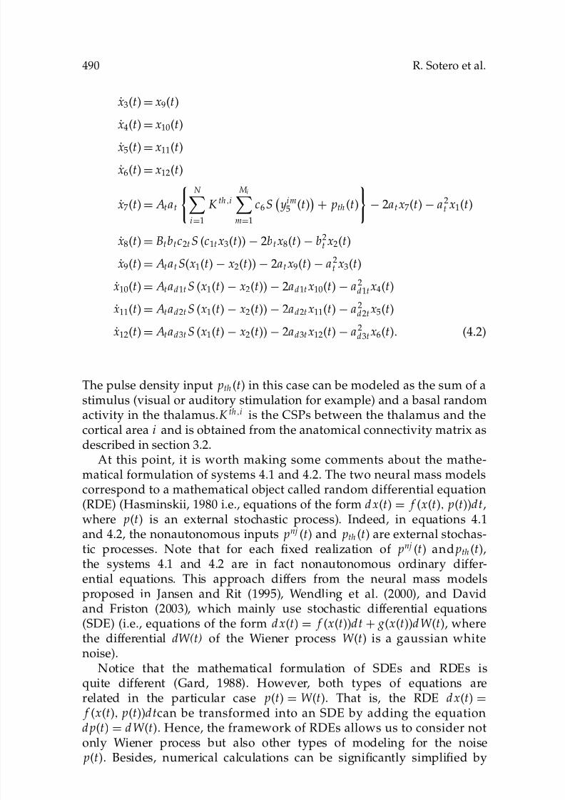
described by the following set of 12 differential equations:

x1(t)= x7(t)

x2(t)= x8(t)




x3(t)= x9(t)

x4(t)= x10(t)

x5(t)= x11(t)

x6(t)= x12(t)

x7(t)= Atat

N

i=1

K th,i Mi

m=1

c6 S yim

5 (t)+ pth (t)

− 2at x7(t)− a 2

t x1(t)

x8(t)= Btbtc2t S (c1t x3(t)) − 2bt x8(t) − b2t x2(t)

x9(t)= Atat S(x1(t) − x2(t))− 2at x9(t) − a 2t x3(t)

x10(t)= Atad1t S (x1(t) − x2(t)) − 2ad1t x10(t) − a 2d1t x4(t)

x11(t)= Atad2t S (x1(t) − x2(t)) − 2ad2t x11(t) − a 2d2t x5(t)

x12(t)= Atad3t S (x1(t) − x2(t)) − 2ad3t x12(t) − a 2d3t x6(t). (4.2)

The pulse density input pth (t) in this case can be modeled as the sum of astimulus (visual or auditory stimulation for example) and a basal random

activity in the thalamus.Kth,i

is the CSPs between the thalamus and thecortical area i and is obtained from the anatomical connectivity matrix asdescribed in section 3.2.

At this point, it is worth making some comments about the mathe-matical formulation of systems 4.1 and 4.2. The two neural mass modelscorrespond to a mathematical object called random differential equation(RDE) (Hasminskii, 1980 i.e., equations of the form d x(t) = f (x(t), p(t))dt,where p(t) is an external stochastic process). Indeed, in equations 4.1and 4.2, the nonautonomous inputs pnj (t) and pth (t) are external stochas-tic processes. Note that for each fixed realization of pnj (t) and pth (t),

the systems 4.1 and 4.2 are in fact nonautonomous ordinary differ-ential equations. This approach differs from the neural mass modelsproposed in Jansen and Rit (1995), Wendling et al. (2000), and Davidand Friston (2003), which mainly use stochastic differential equations(SDE) (i.e., equations of the form dx(t) = f (x(t))dt + g(x(t))dW (t), wherethe differential dW(t) of the Wiener process W (t) is a gaussian whitenoise).

Notice that the mathematical formulation of SDEs and RDEs isquite different (Gard, 1988). However, both types of equations are

related in the particular case p(t) = W (t). That is, the RDE dx(t) = f (x(t), p(t))dtcan be transformed into an SDE by adding the equationdp(t) = dW (t). Hence, the framework of RDEs allows us to consider notonly Wiener process but also other types of modeling for the noise p(t). Besides, numerical calculations can be significantly simplified by




avoiding elements of stochastic integration theory usually required inSDEs.

Finally, the existence and uniqueness of the solution of systems 4.1 and4.2 follow from classical arguments. That is, given a realization of thestochastic processes pnj (t) and pth (t), it is easily seen that the right-handside of systems 4.1 and 4.2 is given by continuously differentiable functionsof their respective arguments (for any choice of the corresponding param-eters). Besides, function S (v(t)) defined in equation 2.3, the only source ofnonlinearity presented on both systems, satisfies a Lipchitz condition (it hasfirst derivative bounded). According to theorem 3.1 in Hasminskii (1980),these two last conditions (continuity and Lipchitz) are enough to guar-antee that our model is well posed (i.e., existence and uniqueness of the

solution).

5 EEG Observation Model

We now relate the average membrane potential of pyramidal cells of eachvoxel to the observed EEG on the scalp surface.

The current dipole due to a PSP is approximately (Hamalainen, Hari,Ilmoniemi, Knuutila, & Lounasmaa, 1993)

j =π

4 d2σ inV = εV (5.1)

ε =π

4d2σ in, (5.2)

where d is the diameter of the dendrite, σ in is the intracellular conductivity,and V is the change of voltage during a PSP (for a single PSP j ≈ 20 fAm;Hamalainen et al., 1993). The equivalent current dipole (ECD) due to N PSPs is then

J =N

i=1

αi ji ≈ ε

N i=1

αiV i , (5.3)

where αi is +1 for EPSP and −1 for IPSP. As discussed in section 2, we canassume that for one voxel.

y1(t) − y2(t) =N

i=1

αiV i (5.4)

and

J (t) = ε ( y1(t) − y2(t)) . (5.5)




On the other hand, from the forward problem of the EEG, we know that thevoltage measured at the scalp surface due to a current density distributionis given by

φ(rs, t) =

K (rs, r g) J (r g, t)d3r g. (5.6)

where the kernel K (rs, r g) is the electric lead field, which summarizes theelectric and geometric properties of the conducting media (brain, skull, and

scalp), and J (r g, t) is the primary current density (PCD) vector. The indicess and g run over the sensor (electrodes) and generator (voxels) spaces,respectively, and t denotes time. The lead field matrix K (rs, r g) is commonly

known and can be calculated by means of the reciprocity theorem (Plonsey,1963; Rush & Driscoll, 1969). Thus, the EEG generated due to the activationof one voxel at a given array of electrodes distributed over the scalp surfacecan easily be calculated by multiplication of the lead field by expression 5.5, both evaluated for the given voxel.

6 Numerical Method

As we mentioned in section 4, an RDE is just a nonautonomous ordinary

differential equation (ODE) coupled with a stochastic process ( p(t) and pth (t) in our model). Thus, in principle, RDEs can be integrated by applyingconventional numerical methods for ODEs. However, it is well known thatclassical methods in ODEs may introduce “ghost” solutions and numericalinstabilities when applied to nonlinear equations, which is critical whendealing with high-dimensional problems (as in our case). On the otherhand, very few researchers have studied systematically the properties ofsuch methods for the numerical integration of RDEs (Grune & Kloeden,2001; Carbonell, Jimenez, Biscay, & de la Cruz, 2005). In this letter wechoose the local linearization (LL) for RDE (Carbonell et al., 2005) to solve

systems 4.1 and 4.2 (see a description of this method in the appendix). Therationale for this choice is the fact that the LL method improves the order ofconvergence and stability properties of conventional numerical integrators(Carbonell et al., 2005) for RDEs. Moreover, the LL approach has been keyfor constructing efficient and stable numerical schemes for the integrationand estimation of various classes of random dynamical systems (Shoji &Ozaki, 1998; Prakasa-Rao, 1999; Schurz, 2002).

7 Results

In this section, computational simulations are used to demonstrate the ca-pability of the model to reproduce the temporal dynamics and spectralcharacteristics of the EEG signal as recorded on the scalp surface. A number of model predictions arising from the results obtained are also shown,




Figure 3: (A) Average anatomical connectivity matrix estimated from diffusionweighted magnetic resonance imaging data of two human subjects. This matrixcontains the connection strength between 71 brain areas. These areas weresegmented based on the Probabilistic Brain Atlas developed at the MontrealNeurological Institute. The values are normalized between 0 and 1. (B) Randommatrix calculated with the same degree of sparseness as that of the anatomicalconnectivity matrix in A.

and can be further tested experimentally. Additionally, the sensitivity of theresults to changes in model parameters is studied.

7.1 Description of the Simulation Method. In the simulations, 71 brainareas were defined based on the Probabilistic MRI Atlas (PMA) produced by the Montreal Neurological Institute (Evans et al., 1993, 1994; Collins,Neelin, Peters, & Evans, 1994; Mazziotta, Toga, Evans, Fox, & Lancaster,1995). Anatomical connectivity matrices between these areas, correspond-ing to two human subjects, were then calculated and averaged out. Theelements of the resultant average matrix were then used as CSP for between-

areas interactions. As shown in Figure 3, the sparseness of this anatomicalconnectivity matrix allows for a significant reduction in the number of CSPsand thus reduces the computational cost of solving the large RDE systemthat describes the model presented here.

Initial conditions were set to zero in all simulations, and an integrationstep size of 5 ms was used. The first 100 points of the simulated signalswere discarded in order to avoid transient behavior, and the input p(t)was a gaussian process with mean and standard deviation of 10,000 and1000 pulses per second, respectively. As for the rest of the model parameter

values, they were chosen to vary across space, with values taken froma uniform distribution in the interval between 5% below and above thestandard values reported in Table 1. This choice was motivated by theinhomogeneities found in cortical tissue. The motor cortex, for example,has a relatively sparse population of neurons, while sensory cortices tend




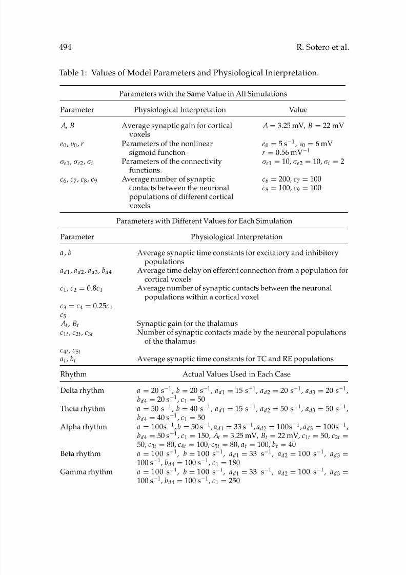
Table 1: Values of Model Parameters and Physiological Interpretation.

Parameters with the Same Value in All Simulations

Parameter Physiological Interpretation Value

A, B Average synaptic gain for corticalvoxels

A= 3.25 mV, B = 22 mV

e0, ν0, r Parameters of the nonlinearsigmoid function

e0 = 5 s−1, ν0 = 6 mVr = 0.56 mV−1

σ e1, σ e2, σ i Parameters of the connectivityfunctions.

σ e1 = 10, σ e2 = 10, σ i = 2

c6, c7, c8, c9 Average number of synapticcontacts between the neuronalpopulations of different corticalvoxels

c6 = 200, c7 = 100c8 = 100, c9 = 100

Parameters with Different Values for Each Simulation

Parameter Physiological Interpretation

a , b Average synaptic time constants for excitatory and inhibitorypopulations

ad1, ad2, ad3, bd4 Average time delay on efferent connection from a population forcortical voxels

c1, c2 = 0.8c1 Average number of synaptic contacts between the neuronalpopulations within a cortical voxel

c3 = c4 = 0.25c1

c5

At , Bt Synaptic gain for the thalamusc1t , c2t , c3t Number of synaptic contacts made by the neuronal populations

of the thalamusc4t , c5t

at , bt Average synaptic time constants for TC and RE populations

Rhythm Actual Values Used in Each Case

Delta rhythm a = 20 s−1, b = 20 s−1, ad1 = 15 s−1, ad2 = 20 s−1, ad3 = 20 s−1,

bd4 = 20 s−1

, c1 = 50Theta rhythm a = 50 s−1, b = 40 s−1, ad1 = 15 s−1, ad2 = 50 s−1, ad3 = 50 s−1,bd4 = 40 s−1, c1 = 50

Alpha rhythm a = 100s−1, b = 50 s−1, ad1 = 33 s−1, ad2 = 100s−1, ad3 = 100s−1,bd4 = 50 s−1, c1 = 150, At = 3.25 mV, Bt = 22 mV, c1t = 50, c2t =50, c3t = 80, c4t = 100, c5t = 80, at = 100, bt = 40

Beta rhythm a = 100 s−1, b = 100 s−1, ad1 = 33 s−1, ad2 = 100 s−1, ad3 =100 s−1, bd4 = 100 s−1, c1 = 180

Gamma rhythm a = 100 s−1, b = 100 s−1, ad1 = 33 s−1, ad2 = 100 s−1, ad3 =100 s−1, bd4 = 100 s−1, c1 = 250




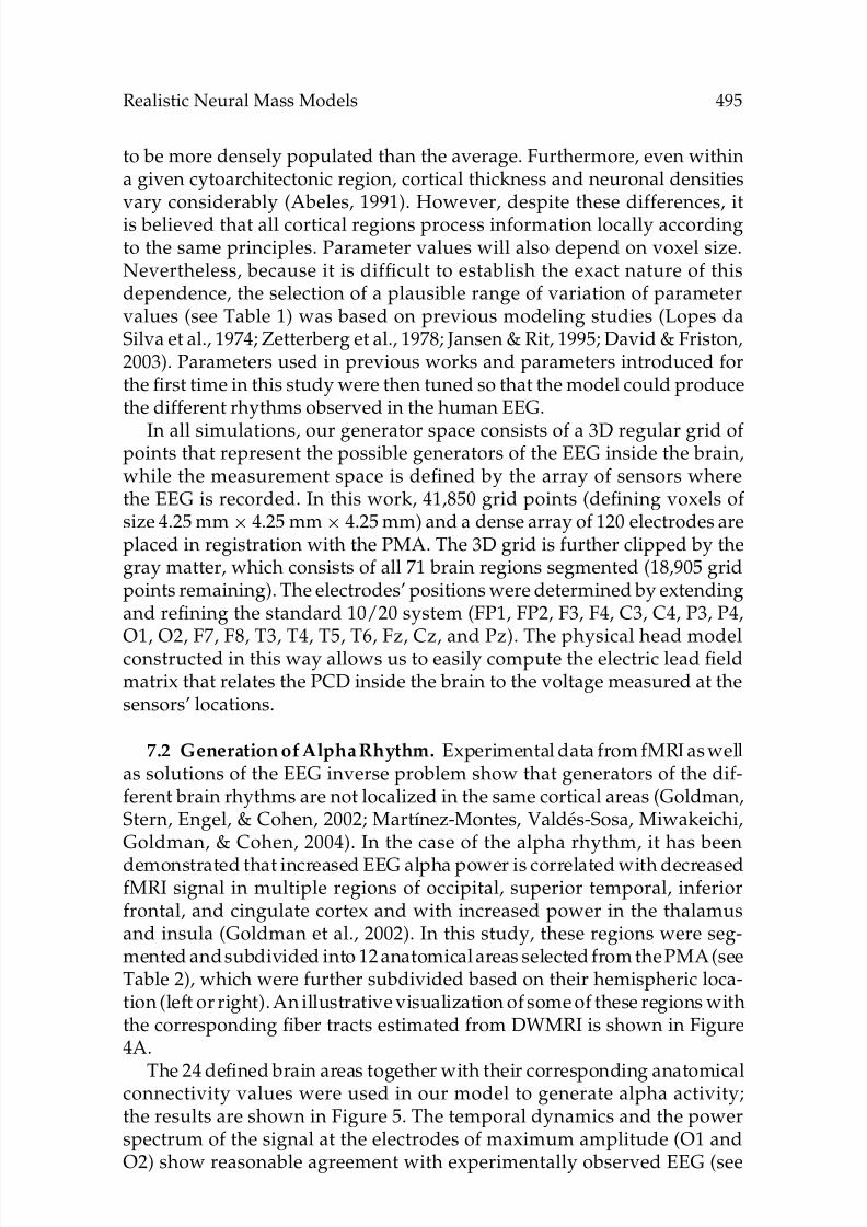
to be more densely populated than the average. Furthermore, even withina given cytoarchitectonic region, cortical thickness and neuronal densitiesvary considerably (Abeles, 1991). However, despite these differences, itis believed that all cortical regions process information locally accordingto the same principles. Parameter values will also depend on voxel size.Nevertheless, because it is difficult to establish the exact nature of thisdependence, the selection of a plausible range of variation of parametervalues (see Table 1) was based on previous modeling studies (Lopes daSilva et al., 1974; Zetterberg et al., 1978; Jansen & Rit, 1995; David & Friston,2003). Parameters used in previous works and parameters introduced forthe first time in this study were then tuned so that the model could producethe different rhythms observed in the human EEG.

In all simulations, our generator space consists of a 3D regular grid ofpoints that represent the possible generators of the EEG inside the brain,while the measurement space is defined by the array of sensors wherethe EEG is recorded. In this work, 41,850 grid points (defining voxels ofsize 4.25 mm × 4.25 mm× 4.25 mm) and a dense array of 120 electrodes areplaced in registration with the PMA. The 3D grid is further clipped by thegray matter, which consists of all 71 brain regions segmented (18,905 gridpoints remaining). The electrodes’ positions were determined by extendingand refining the standard 10/20 system (FP1, FP2, F3, F4, C3, C4, P3, P4,

O1, O2, F7, F8, T3, T4, T5, T6, Fz, Cz, and Pz). The physical head modelconstructed in this way allows us to easily compute the electric lead fieldmatrix that relates the PCD inside the brain to the voltage measured at thesensors’ locations.

7.2 Generation of Alpha Rhythm. Experimental data from fMRI as wellas solutions of the EEG inverse problem show that generators of the dif-ferent brain rhythms are not localized in the same cortical areas (Goldman,Stern, Engel, & Cohen, 2002; Martınez-Montes, Valdes-Sosa, Miwakeichi,Goldman, & Cohen, 2004). In the case of the alpha rhythm, it has been

demonstrated that increased EEG alpha power is correlated with decreasedfMRI signal in multiple regions of occipital, superior temporal, inferiorfrontal, and cingulate cortex and with increased power in the thalamusand insula (Goldman et al., 2002). In this study, these regions were seg-mented andsubdivided into 12 anatomical areas selected from the PMA (seeTable 2), which were further subdivided based on their hemispheric loca-tion (left or right). An illustrative visualization of some of these regions withthe corresponding fiber tracts estimated from DWMRI is shown in Figure4A.

The 24 defined brain areas together with their corresponding anatomicalconnectivity values were used in our model to generate alpha activity;the results are shown in Figure 5. The temporal dynamics and the powerspectrum of the signal at the electrodes of maximum amplitude (O1 andO2) show reasonable agreement with experimentally observed EEG (see




Table 2: Brain Areas Selected for Each Rhythm Simulation.

Alpha Rhythm Delta, Beta, Theta, and Gamma Rhythms

Cuneus (left and right) Medial front-orbital gyrus (left and right)Lingual gyrus (left and right) Middle frontal gyrus (left and right)Lateral occipitotemporal gyrus (left and

right)Precentral gyrus (left and right)

Insula (left and right) Lateral front-orbital gyrus (left and right)Inferior occipital gyrus (left and right) Medial frontal gyrus (left and right)Superior occipital gyrus (left and right) Superior frontal gyrus (left and right)Medial occipitotemporal gyrus (left and

right)Inferior frontal gyrus (left and right)

Occipital pole (left and right)

Cingulate region (left and right)Inferior frontal gyrus (left and right)Superior temporal gyrus (left and right)Thalamus (left and right)

Figure 4: Visualization of the fiber tracts connecting the brain regions used inthe simulations as calculated from DWMRI. (A) Alpha rhythm: left and rightsuperior temporal gyri (1, 2); left and right thalamus (3, 4); left and right medial

occipitotemporal gyri (5, 6); left and right occipital poles (7, 8). (B) Beta, gamma,delta, and theta rhythms: left and right superior frontal gyri (1, 2); left and rightinferior frontal gyri (3, 4).




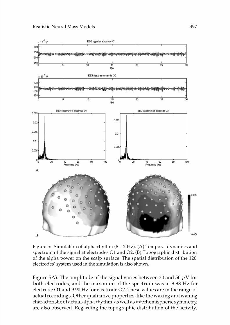
Figure 5: Simulation of alpha rhythm (8–12 Hz). (A) Temporal dynamics andspectrum of the signal at electrodes O1 and O2. (B) Topographic distributionof the alpha power on the scalp surface. The spatial distribution of the 120electrodes’ system used in the simulation is also shown.

Figure 5A). The amplitude of the signal varies between 30 and 50 µV for

both electrodes, and the maximum of the spectrum was at 9.98 Hz forelectrode O1 and 9.90 Hz for electrode O2. These values are in the range ofactual recordings. Other qualitative properties, like the waxing and waningcharacteristic of actual alpha rhythm, as well as interhemispheric symmetry,are also observed. Regarding the topographic distribution of the activity,




Figure 6: Reactivity test simulation. A trapezoidal input of 12 seconds durationand amplitude of 106 pulses per second is used to simulate visual input at thethalamic level. The response of the system results in a significant reduction inthe amplitude of both the signal and the peak of the alpha power and a shift ofthe power spectrum toward higher frequencies.

Figure 5B shows that the simulated EEG is maximal over the occipitalregions and diminishes in amplitude toward frontal areas, which has also been described for alpha rhythm.

The influence of an external input (stimulus) on the simulated alphaactivity was also studied, and results are depicted in Figure 6. Actualalpha rhythm is known to be temporarily blocked by an influx of light(eye opening). This is known as reactivity. The degree of reactivity varies;the alpha rhythm may be blocked, suppressed, or attenuated with voltage




reduction (Niedermeyer & Lopes da Silva, 1987). In the simulations shownin Figure 6, a trapezoidal input representing visual stimulation of 12 sec-onds duration and amplitude of 106pulses per second was given to thethalamus. As shown in the figure, the effect of this input was to attenuatethe EEG signal and shift the whole EEG spectrum toward higher frequen-cies with a reduction in the amplitude of the power, which is also observedin actual reactivity tests.

7.3 Generation of Delta, Theta, Beta, and Gamma Rhythms. For thesimulation of delta, theta, beta, and gamma rhythms, 7 brain regions(medial-front orbital gyrus, middle frontal gyrus, precental gyrus, lateral-

front orbital gyrus, medial frontal gyrus, superior frontal gyrus, and inferiorfrontal gyrus) were selected and subdivided based on their hemispheric lo-cation (left or right), for a total of 14 brain areas. Some of these areas, withthe corresponding fiber tracts connecting them, are shown in Figure 4B.

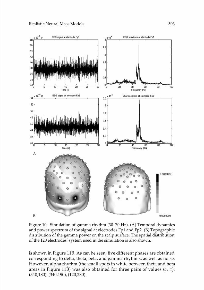
In these studies, 30 seconds of EEG data were simulated for each rhythm.Figures 7, 8, 9, and 10 show the temporal dynamics and the spectrum ofthe signal obtained at electrodes Fp1 and Fp2 for the delta, theta, beta,and gamma rhythms simulations, respectively. Amplitudes and spectralfrequency bands obtained are within the range of experimentally observedEEG. Note the characteristic interhemispheric asymmetry in the frequency

of the peak for the beta rhythm (see Figure 9). That is, the maximum ofthe spectrum is located at 18.46 Hz for electrode Fp1 and at 16.76 Hz forelectrode Fp2. The rest of the simulated rhythms do not show a significantinterhemispheric frequency asymmetry. Finally note that the power spec-trum on the scalp surface was maximum at frontal areas in all cases andreaches minimum amplitudes at occipital electrodes.

7.4 Influence of the Model Parameters on the Generation of the EEGRhythms. Parameter values in Table 1 show that by increasing c1 (and thus

c2, c3, and c4), while keeping the other parameters constant, the EEG spec-trum shifts toward higher frequencies, going from beta to gamma frequency bands. On the other hand, keeping c1 constant, we can switch from deltato theta rhythm by increasing parameters associated with membrane timeconstants and dendritic tree time delays. However, as there are 32 param-eters in the model (excluding the connectivity matrix values), it is difficultto study the influence of each of them on the output of the model. Thatis, parameter values presented in Table 1 are not the only ones capable ofproducing EEG rhythms. Additionally, neural mass models can produce

the same EEG rhythm with different sets of parameter values, as shown byDavid and Friston (2003), which varied excitatory and inhibitory time con-stants and obtained regions of the parameters’ phase-space within whichthe same rhythm was obtained. In this section, we perform similar analysesfor parameters a and b.




Figure 7: Simulation of delta rhythm (1–4 Hz). (A) Temporal dynamics andpower spectrum of the signal at electrodes Fp1 and Fp2. (B) Topographic dis-tribution of the delta power on the scalp surface. The spatial distribution of the120 electrodes’ system used in the simulation is also shown.

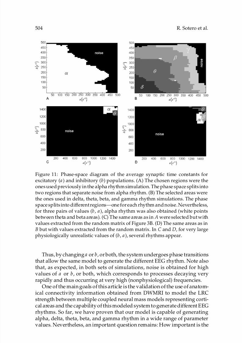
In the first set of simulations the areas involved in the alpha rhythmsimulation study were selected, and then parameters a , b were varied from10 s−1 to 500 s−1, with a step size of 10 s−1, while the rest of the parameterswere kept constant with the values in Table 1 that correspond to alpharhythm. For each case, the resulting dynamics was assigned to an EEG




Figure 8: Simulation of theta rhythm (4–8 Hz). (A) Temporal dynamics andpower spectrum of the signal at electrodes Fp1 and Fp2. (B) Topographic dis-tribution of the theta power on the scalp surface. The spatial distribution of the120 electrodes’ system used in the simulation is also shown.

band. A phase diagram is shown in Figure 11A. Two phases are obtaineddepending on parameter values: one corresponding to alpha rhythms andthe other corresponding to noise.




Figure 9: Simulation of beta rhythm (12–30 Hz). (A) Temporal dynamics andpower spectrum of the signal at electrodes Fp1 and Fp2. (B) Topographic dis-tribution of the theta power on the scalp surface. The spatial distribution of the120 electrodes’ system used in the simulation is also shown.

In the second study, parameters a , b were also varied from 10 s−1

to500 s−1 with a step size of 10 s−1, but now the brain areas selected were theones involved in the generation of delta, theta, beta, and gamma rhythms.As in the previous case, the other parameters were kept constant with thevalues shown in Table 1 for beta rhythm. The corresponding phase diagram




Figure 10: Simulation of gamma rhythm (30–70 Hz). (A) Temporal dynamicsand power spectrum of the signal at electrodes Fp1 and Fp2. (B) Topographicdistribution of the gamma power on the scalp surface. The spatial distributionof the 120 electrodes’ system used in the simulation is also shown.

is shown in Figure 11B. As can be seen, five different phases are obtainedcorresponding to delta, theta, beta, and gamma rhythms, as well as noise.However, alpha rhythm (the small spots in white between theta and betaareas in Figure 11B) was also obtained for three pairs of values (b, a ):(340,180), (340,190), (120,280).




Figure 11: Phase-space diagram of the average synaptic time constants for

excitatory (a) and inhibitory (b) populations. (A) The chosen regions were theones used previously in the alpha rhythm simulation. The phase space splits intotwo regions that separate noise from alpha rhythm. (B) The selected areas werethe ones used in delta, theta, beta, and gamma rhythm simulations. The phasespace splits into different regions—one for each rhythm and noise. Nevertheless,for three pairs of values (b, a), alpha rhythm was also obtained (white points

between theta and beta areas). (C) The same areas as in A were selected but withvalues extracted from the random matrix of Figure 3B. (D) The same areas as inB but with values extracted from the random matrix. In C and D, for very largephysiologically unrealistic values of (b, a), several rhythms appear.

Thus, by changing a or b, or both, the system undergoes phase transitionsthat allow the same model to generate the different EEG rhythm. Note alsothat, as expected, in both sets of simulations, noise is obtained for highvalues of a or b, or both, which corresponds to processes decaying veryrapidly and thus occurring at very high (nonphysiological) frequencies.

One of the main goals of this article is the validation of the use of anatom-ical connectivity information obtained from DWMRI to model the LRC

strength between multiple coupled neural mass models representing corti-cal areas and the capability of this modeled system to generate different EEGrhythms. So far, we have proven that our model is capable of generatingalpha, delta, theta, beta, and gamma rhythm in a wide range of parametervalues. Nevertheless, an important question remains: How important is the




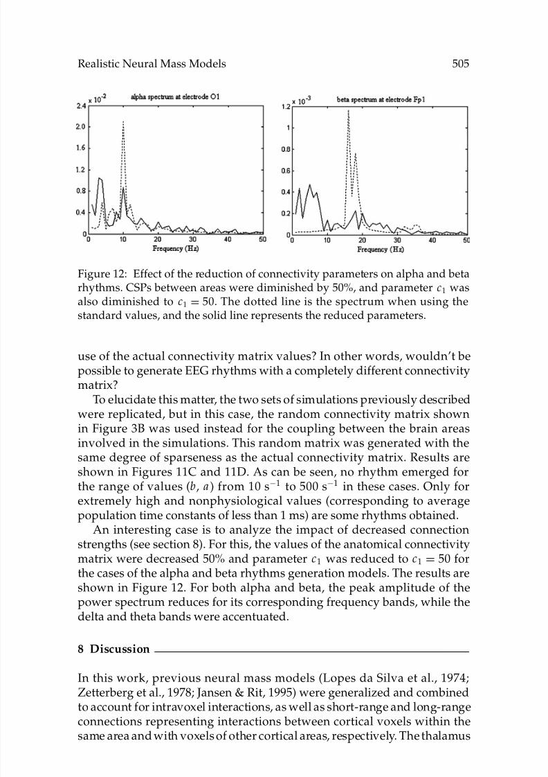
Figure 12: Effect of the reduction of connectivity parameters on alpha and betarhythms. CSPs between areas were diminished by 50%, and parameter c1 wasalso diminished to c1 = 50. The dotted line is the spectrum when using thestandard values, and the solid line represents the reduced parameters.

use of the actual connectivity matrix values? In other words, wouldn’t bepossible to generate EEG rhythms with a completely different connectivitymatrix?

To elucidate this matter, the two sets of simulations previously describedwere replicated, but in this case, the random connectivity matrix shownin Figure 3B was used instead for the coupling between the brain areasinvolved in the simulations. This random matrix was generated with thesame degree of sparseness as the actual connectivity matrix. Results areshown in Figures 11C and 11D. As can be seen, no rhythm emerged forthe range of values (b, a ) from 10 s−1 to 500 s−1 in these cases. Only forextremely high and nonphysiological values (corresponding to averagepopulation time constants of less than 1 ms) are some rhythms obtained.

An interesting case is to analyze the impact of decreased connection

strengths (see section 8). For this, the values of the anatomical connectivitymatrix were decreased 50% and parameter c1 was reduced to c1 = 50 forthe cases of the alpha and beta rhythms generation models. The results areshown in Figure 12. For both alpha and beta, the peak amplitude of thepower spectrum reduces for its corresponding frequency bands, while thedelta and theta bands were accentuated.

8 Discussion

In this work, previous neural mass models (Lopes da Silva et al., 1974;Zetterberg et al., 1978; Jansen & Rit, 1995) were generalized and combinedto account for intravoxel interactions, as well as short-range and long-rangeconnections representing interactions between cortical voxels within thesame area and with voxels of other cortical areas, respectively. The thalamus




was also described by a neural mass model and coupled to the cortical areas.Anatomical information from DWMRI was introduced to constrain cou-pling strength parameters between different brain regions. This allowed usto couple multiple brain areas with real anatomical connectivity values andstudy the rhythms emerging from these interactions across different spatialscales. Knowing the average depolarization of pyramidal cells in each voxeland the lead field matrix that characterizes the spatial distribution of theelectromagnetic field in the head, we obtained the voltage signals recordedat the location of given electrodes on the scalp surface.

For validating the model, several simulations were carried out. The pa-rameters that were tuned in each simulation were the time delays of efferentconnections and connectivity constants between the different populations

within a voxel. The choice of parameter was given by its importance inthe generation of different rhythms, as demonstrated by previous work inthis field (Jansen & Rit, 1995; David & Friston, 2003). The temporal dy-namics and the spectrum of human EEG rhythms were reproduced by theproposed model. EEG rhythms were also obtained at the right spatial lo-cations. In the case of alpha rhythm, the activity was maximal at occipitalelectrodes and diminished toward the frontal electrodes. Delta, theta, beta,and gamma rhythms were maximal at frontal electrodes. The amplitudesof the rhythms were also within the range observed in actual EEG record-

ings. Interhemispheric symmetry was found in the case of alpha rhythm,since the difference between the peaks of EEG spectrum at electrodes O1and O2 was less than 0.1 Hz. In contrast beta rhythm showed interhemi-spheric asymmetry; that is, there was a difference of 1.7 Hz between thepeaks of the EEG spectrum at Fp1 and Fp2. For delta, theta, and gammarhythms, interhemispheric symmetry with respect to the peak frequency ofthe spectrum was obtained. In clinical practice, no EEG is complete with-out a reactivity test (Niedermeyer & Lopes da Silva, 1987). For this reason,we made a reactivity test simulation, finding that the effect of stimulationwas to shift the spectrum toward higher frequencies together with a reduc-

tion in amplitude, which also agrees with actual EEG recordings in healthysubjects.

Instead of the anatomical connectivity matrix, values from a randommatrix were also used to couple brain areas. In this case, some rhythmsappear for extremely high values of parameters a and b. However, thesevalues of a and b correspond to an average population time constant of lessthan 1 ms, which does not make much sense from the physiological point ofview. Thus, it can be concluded that in the range of physiologically plausiblevalues, no rhythm was obtained when using a nonrealistic connectivity

matrix.Finally, the model was used to study the effect of a reduction in all

connectivity parameters values predicting an increase in delta and thetapower (see Figure 12), along with a decrease in alpha and beta peaks. It is




interesting to note that this slowing of oscillatory activity is a prominentfunctional abnormality that has been reported in EEG and MEG studies ofAlzheimer disease (AD) patients (Coben, Danziger, & Berg, 1983; Penttila,Partanen, Soininen, & Riekkinen, 1985; Schreiter-Gasser, Gasser, & Ziegler,1993; Berendse, Verbunt, Scheltens, van Dijk, & Jonkman, 2000). On theother hand it is also recognized that AD patients show a progressive corti-cal disconnection syndrome due to the loss of large pyramidal neurons incortical layers III and V (Pearson, Esiri, Hiorns, Wilcock, & Powell, 1985;Morrison, Scherr, Lewis, Campbell, & Bloom, 1986). Related to this, it hasalso been found that the total callosal area is significantly reduced in pa-tients suffering from this pathology (Rose et al., 2000; Hampel et al., 1998).According to our model, the shift of the EEG spectrum toward low fre-

quencies found in AD could be associated with the cortical disconnectionsyndrome that is reflected in the decreased values of the coupling strengthparameters, although the model does not exclude contributions from othermechanisms.

As we know, lumped models are simplifications of actual brain struc-tures, so further improvements could be made by including more realisticmodels in order to describe a wider range of phenomena. Another limita-tion of our approach is that DWMRI cannot distinguish between efferentand afferent fibers (this is reflected in the symmetry of the connectivity

matrix; see Figure 3A), and connectivity values thus could be overesti-mated. Moreover, the validity of the connectivity matrix values dependson the assumption that probabilistic paths calculated based on the infor-mation obtained from DWMRI reflect the actual connections between brainareas.

While this letter focused on the EEG forward problem, the next logicalstep is the estimation of the parameters of this model from data. Previouswork has accomplished this task. For example, in Valdes et al. (1999), theneural mass model described in Zetterberg et al. (1978) was fitted to actualEEG alpha data. In that work, the LL approach was used to discretize Zetter-

berg’s model, which was then reformulated in a state-space formalism thatcould be integrated by using a nonlinear Kalman filter scheme. A maximumlikelihood procedure was then employed to estimate the model parametersfor several EEG data sets. Bayesian inference, dynamic causal modeling(Friston, Harrison, & Penny, 2003; David, Harrison, Kilner, Penny, & Fris-ton, 2004), and genetic algorithms (Jansen, Balaji Kavaipatti, & Markusson,2001) have also been used for estimating the parameters of neural massmodels of the type presented here. A more ambitious goal is the integrationof EEG with functional imaging techniques such as functional magnetic res-

onance imaging and positron emission tomography. The use of this modelas a framework in which electrical, hemodynamic, and metabolic activitiescan be coupled is currently under study and will be the subject of a futurepublication.




Appendix: Local Linearization Method for RDE

Assume that a k-dimensional random process p(t), t ∈ [t0, T ] and a non-linear function f are given, and define the d-dimensional RDE:

d y(t)= f ( y(t), p(t))dt

y(t0)= y0.

Then, given a step size h,the local linearization scheme that solves numer-ically the equation above at the time instants tn = t0 + nh,n = 0, 1, . . . , isgiven by

yn+1 = yn + LeCnh R,

where L = [I d , 0d x2], R = [01x(d+1), 1]T , and the (d + 2) × (d + 2) matrix Cn

is defined by blocks as

Cn =

˙ f y(t)( yn, p(tn)) ˙ f p(t)( yn, p(tn)) p(tn+1)− p(tn)h

f ( yn, p(tn))0 0 10 0 0

Here, ˙ f y(t)and ˙ f p(t) denote the derivatives of f with respect to the variables y and p, respectively.

Due to the high dimensionality of our problem, the main task in the im-plementation of the LL scheme is the computation of the matrix exponentialeCnh . The use of the Krylov subspace methods (Sidje, 1998) is strongly rec-ommended for that purpose. Indeed, that method can be used to computethe vector v = eCnh R, and then the operation Lv reduces to take the first delements of v.

Acknowledgments

We thank Trinidad Virues, Elena Cuspineda, and Thomas Wennekers forhelpful comments.

References

Abeles, M. (1991). Corticonics: Neural circuits of the cerebral cortex. Cambridge:

Cambridge University Press.

Behrens, T., Johansen-Berg, H., Woolrich, M. W., Smith, S. M., Wheeler-Kingshott, C., Boulby, P. A., Barker, G. J., Sillery, E. L., Sheehan, K., Ciccarelli, O.,

Thompson, A. J., Brady, J. M., & Matthews, P. M. (2003). Non-invasive mapping

of connections between human thalamus and cortex using diffusion imaging.

Nature Neuroscience, 6, 750–757.

Realistically Coupled Neural Mass Models Can Generate EEG Rhythms

Documents

Transcript of Realistically Coupled Neural Mass Models Can Generate EEG Rhythms