Real Options, Irreversible Investment and Firm Uncertainty...

1

Real Options, Irreversible Investment and Firm Uncertainty:

New Evidence from U.S. FirmsLaarni T. Bulan*†

September 2004

JEL Classification: G31Keywords: Real Options, Irreversible Investment

Abstract

This paper investigates real options behavior in capital budgeting decisions using a firm-level

panel data set of U.S. companies in the manufacturing sector. Specifically, this paper looks are

the relationship between the firm’s investment to capital ratio and total firm uncertainty,

measured as the volatility of the firm’s equity returns. Total firm uncertainty is decomposed into

its market, industry and firm-specific components. Given that the irreversibility of capital is

derived from asset-specificity at the industry level, increased industry uncertainty displays a

pronounced negative effect on firm investment consistent with real options behavior. Increased

firm-specific uncertainty is also found to depress firm investment - a result that can be attributed

to real options behavior and not just managerial risk aversion. The results are robust to various

specifications that control for the firm’s investment opportunities that are captured by Tobin’s q,

cash flow, marginal profitability of capital and firm leverage.

*Assistant Professor, Brandeis University International Business School, 415 South Street MS 021, Waltham, MA

02454, USA Phone: 781-736-2294 Fax: 781-736-2269 Email: [email protected]

† I am indebted to Charlie Himmelberg, Chris Mayer, John Donaldson, Larry Glosten, and Ken Kuttner for their

guidance and support. I would also like to thank Andrew Ang, Blake Le Baron, Chris Downing, Ray Fisman,

Dominika Halka, Cornelia Kullmann, Inessa Love, Deborah Lucas, Robert McDonald, Marti Subrahmanyam,

Narayanan Subramanian, Zhenyu Wang, Karl Whelan, Atakan Yalcin, John Yeoman and three anonymous referees

for helpful comments and suggestions. All remaining errors are mine.

1McDonald and Siegel (1986) present a tractable solution to the valuation of an option to invest in an

irreversible project. Similar problems are also investigated in Baldwin (1982), Bernanke (1983) and McDonald and

Siegel (1985). Titman (1985) specifically focuses on the valuation of land while Brennan and Schwartz (1985)

evaluate investments in natural resource projects.

2See McDonald and Siegel (1986), Pindyck (1988) and Dixit and Pindyck (1994). Homogeneous capital

goods that are not industry or firm-specific (such as office equipment) are still partially irreversible because of the

lemons problem. Abel and Eberly (1994, 1996) and Abel, Dixit, Eberly and Pindyck (1996) define partial

irreversibility (or costly reversibility) as the case when the purchase price of capital is greater than its resale price.

2

I. INTRODUCTION

What is it about real options that has made it a buzz word on the Street? Why is it that

real options theory has caught the attention of academics and practitioners alike? In a survey of

corporate finance practices in the U.S., Graham and Harvey (2001) find that more than 70 % of

the CFOs surveyed rely on discounted cash flows and the Capital Asset Pricing Model (CAPM)

for their capital budgeting decisions. Despite the popularity of Net Present Value (NPV), it has

long been acknowledged that it fails to capture an important feature of the investment decision -

that of managerial flexibility in a dynamic and uncertain environment. Among the various

methods that have been devised to address this shortcoming of the NPV model, the use of

option-pricing techniques holds the most promise. In contrast to the static NPV invest-now-or-

never rule, real option methods maximize the value of the investment opportunity, i.e. maximize

the value of a call option.1

The ability to delay investment decisions is valuable when the investment is irreversible

and the future is uncertain. The irreversibility of investment expenditures stems from capital

specificity at the industry level and/or at the firm level.2 If managers can wait for the resolution

3

of uncertainty before deciding to pursue the irreversible investment, they can avoid potentially

large losses by foregoing the investment altogether when the outcome is unfavorable. Hence, a

familiar result from option-pricing applies to irreversible investments: the greater the uncertainty

in an investment’s expected future cash flows, the more valuable is this option to delay the

investment. This in turn reduces the incentive for exercising the option today.

This paper investigates real options behavior in capital budgeting decisions of U.S.

companies in the manufacturing sector. In particular, this paper tests whether real options

models can explain the relationship between firm investment and uncertainty. Although a

majority of firms may not actually be employing real options techniques yet, McDonald (2000)

points out that arbitrary methods such as hurdle rates and profitability indexes can actually

approximate the optimal decision under real options, i.e. the same factors that increase the value

of the option to delay investment also increase firm hurdle rates and profitability requirements.

By improving on the empirical methods of prior studies, this paper provides substantial

evidence at the firm-level and makes two significant contributions towards finding support for

real options behavior of firm managers. First, the approach taken in this paper is to use an

“asset-pricing” model to decompose the total uncertainty faced by an individual firm into its

systematic and firm-specific components and then relate these measures to the firm’s

investment behavior. The traditional view asserts that it is only systematic risk (e.g. market

uncertainty under the CAPM), as it affects the firm’s cost of capital, that should matter for firm

investment. Real options models predict the contrary, that it is total risk or total firm uncertainty

that should matter for firm investment. By decomposing risk in this manner, we can identify

whether firm-specific risk adds value through the firm’s investment (or growth) options and

hence, identify whether it influences investment decisions. Second, in addition to a market

3Consider the case where a single firm experiences a negative shock to its profits. Since other firms in the

industry are not affected by this shock, the resale value of this firm’s capital is high. On the other hand, if the

negative shock were industry-wide, then the resale value of its capital would be much lower because all firms in the

industry are adversely affected.

4These calculations are based on the mean investment-to-capital ratio.

5Only two other papers have looked at the effect of competition on investment behavior in a real options

framework at the firm or project level: Guiso and Parigi (1999) and Bulan, Mayer and Somerville (2003).

4

component, total firm uncertainty is decomposed further to account for the effect of industry-

wide variations. Distinguishing between industry uncertainty and firm-specific uncertainty is

important for irreversible investments. Dixit and Pindyck (1994) argue that the irreversibility of

capital is more pronounced at the industry level because capital is industry-specific.3 In this

case, the predictions of real options theory have greater relevance for uncertainty that is industry-

wide.

This paper provides empirical support for the prediction of real options models that

higher uncertainty reduces incentives for investing. The decomposition of total uncertainty into

its market, industry and firm-specific components reveals that periods of higher industry and

firm-specific uncertainty are related to lower investment by firms. A one standard deviation

increase in industry uncertainty reduces a firm’s investment-to-capital ratio by 6.4 %. A one

standard deviation increase in firm-specific uncertainty decreases firm investment by 19.3 %. In

contrast, a one standard deviation increase in Tobin’s q increases investment by only 5 %.4 The

findings point to the importance of industry uncertainty as a determinant of firm investment

when capital is industry specific.

In addition, this paper revisits the effect of competition on investment behavior.5

6See for example Federer (1993), Pindyck & Solimano (1993), Huizinga (1993), Caballero & Pindyck

(1996), Holland, Ott & Riddiough (2000), and Ghosal and Loungani (1996, 2000).7See for example, Paddock, Siegel and Smith (1988), Quigg (1993), Favero, Pesaran & Sharma (1994),

Hurn and Wright (1994), Moel and Tufano (2002) and Bulan, Mayer and Somerville (2003).

5

Competition has a differential effect on the investment-uncertainty relationship. This finding

provides further evidence for real options behavior and precludes managerial risk aversion as an

alternative interpretation of the results.

The remainder of the paper is organized as follows. Section II reviews related empirical

studies. Section III presents the empirical model used in the estimation and provides a

description of the data. Section IV gives the empirical results and Section V concludes.

II. RELATED LITERATURE

Few papers have attempted to empirically test the investment-uncertainty relationship

predicted by irreversible investment models. The evidence has not been completely supportive

of the implication that higher uncertainty discourages firm investment. Studies that have been

successful in documenting a negative influence of uncertainty on investment have mainly used

aggregate data.6 It is unclear, however, if the same conclusions from real options theory derived

at the firm or project level can be made at the macro level or even at the industry level. These

papers can only infer real options behavior from the relationship between the level of investment

and uncertainty. On the other hand, studies that use project level data have been able to

investigate the effect of uncertainty on the timing (as opposed to the level) of investment, which

is a direct test of the optimal exercise of real options. These project-level studies however have

mixed findings7. A third line of inquiry in the empirical literature utilizes firm-level data such as

6

Bell & Campa (1997), Leahy and Whited (1996) and Guiso and Parigi (1999).

Most relevant to this paper is the study by Leahy & Whited (1996). They use a panel of

manufacturing firms from Compustat and CRSP to document some stylized facts regarding the

relationship between investment and uncertainty over the period 1981-1987. They employ VAR

methods to generate volatility forecasts from daily stock returns to measure uncertainty. They

control for Tobin’s q in their main regressions and include the covariance of equity returns with

the market return to test the implications of the CAPM for firm investment. Their main finding

is that the variance of stock returns has a negative effect on investment that works primarily

through Tobin’s q, i.e. once they control for Tobin’s q, the variance of equity returns has no

predictive power for investment. In addition, they find no evidence that their CAPM-based

measure of risk plays a role in the investment decision.

At the firm level the evidence is weak. At the project level, support for real options

behavior is more favorable. Nevertheless project level studies remain specific to certain

industries (e.g. real estate and mining) and generalizing their findings to other industries may not

be straightforward. This paper attempts to provide stronger support for real options models at

the firm level by analyzing a heterogenous group of firms from the U.S. manufacturing sector

and improving on the empirical methods of previous work.

III. EMPIRICAL SPECIFICATION

A. Measuring Uncertainty

Obtaining a general measure of the uncertainty affecting a firm is not straightforward.

Many theoretical models require a measure of the volatility of a firm’s demand shocks or more

precisely, the volatility of a firm's output price. Other models have also included uncertainty in

8Volatility is measured over a firm’s fiscal year to correspond with reported financial data.

7

input costs or supply-side shocks. As an alternative, the measure of uncertainty employed in this

paper is the volatility of a firm’s stock returns. The advantage of this measure is that it captures

the total uncertainty that is relevant to the firm in a single variable, facilitating a decomposition

of risk into its various components as discussed below. Pindyck (1991) argues that increased

volatility in the product markets is translated into increased volatility in the stock market. Leahy

and Whited (1996) reason that stock returns capture the changing aspects of a firm’s

environment that is important to investors. Additionally, Berk, Green and Naik (1999) show that

time variation in asset returns are driven by the firm’s expectations about its returns from assets

in place and from potential growth options. Simply put, common stock represents claims on the

future profits of a firm. Innovations to a firm’s stock return are reactions to news about the

firm’s future profitability and future investment opportunities. If markets are efficient, news

about asset fundamentals and the firm’s future prospects are priced by the market. Hence, the

volatility of a firm’s stock returns should reflect these variations and provide an adequate

measure of the total uncertainty that is relevant for firm-level investment decisions.

Total firm uncertainty for firm i in year t is measured as the volatility of the firm’s equity

returns, i.e. the annualized standard deviation of the firm’s daily returns in that fiscal year, .8 $σ it

Daily returns are used to generate annual volatility measures from non-overlapping samples of

return data. This creates an estimation error in that is uncorrelated over time, which is its$σ it

advantage over moving-average procedures for calculating volatility that use lower frequency

9Daily returns however are noisy and can capture changes in non-fundamentals. This noise will be factored

into measurement error in . $σ it

10All volatility measures are annualized by multiplying by the square-root of 252 (the number of trading

days in a year).

8

data. In addition, small sample bias is also minimized.9

Total uncertainty is decomposed into its aggregate and firm-specific components by

estimating the following two-index model. Under the standard i.i.d assumptions for returns in

each year,

, (1)r r ri it it M it I iτ τ τ τα β γ ε= + + +

where J = 1, 2, ..., ti . ti is the number of trading days in year t, is the daily return on firmriτ

i’s equity, is the daily return on the market index, is the component of the daily returnrMτ rIτ

on firm i’s industry index that is orthogonal to the market return, and is a white noise errorε it

term with variance . and are the market and industry betas respectively for firm iσ εit β it γ it

in year t, as implied by this two-index model. Using ordinary-least-squares, the estimated betas

are and . The resulting standard deviation of residuals from this regression, , is the$β it $γ it$σ εit

estimate of firm-specific uncertainty.10 This measure captures the volatility of returns that is

orthogonal to both market and industry movements.

Denote the annual volatility of market returns by and the volatility of industry$σ Mt

11It can be argued that alternative asset pricing models will yield different measures of firm-specific

uncertainty, such as the Fama-French three-factor model. The choice of risk decomposition in this paper is clearly

motivated from a statistical framework and is based on 1) Dixit and Pindyck (1994) and 2) the straightforward

economic interpretation of the results from a real investment perspective. As a robustness check, the Fama-French

three-factor model is used and similar results are found in terms of the relationship between firm investment and

firm-specific uncertainty. The difficulty arises in the interpretation of the results for the three “systematic” factor

risks and their role in firm investment behavior.

12It is possible that the individual risk components of stock return volatility may not correspond to the true

systematic and unsystematic risks that the firm faces due to the fact that stock return volatility is dependent on the

degree of “moneyness” of a firm’s real options. To address this issue, measures of total uncertainty, market

uncertainty and industry uncertainty are constructed similar to Leahy and Whited (1996). (Instead of a risk

9

returns for industry I in year t that is orthogonal to the market return by . Using the$σ It

estimated beta from equation (1), market uncertainty is measured as , i.e. the portion of$ $β σit Mt

total market uncertainty that matters for the firm. Similarly, industry uncertainty for firm i in

industry I is measured as , i.e. the portion of total industry uncertainty that is relevant to$ $γ σit It

the firm and orthogonal to market movements.

For comparison, an alternative decomposition of uncertainty is estimated where the

restriction is imposed on equation (1). This scenario is analogous to the Capital Assetγ it = 0

Pricing Model (CAPM) and provides a benchmark for comparing the value-added of identifying

industry sources of uncertainty. In particular, it allows a test of the hypothesis that the type of

uncertainty that impacts valuation when capital is irreversible stems from capital-specificity at

the industry level.11,12

decomposition, Leahy and Whited include total stock return volatility and the covariance of a firm’s stock return

with the market return.) With these alternative measures of uncertainty, the findings in section IV are unchanged.

13The shortcoming of this scaling is that it assumes debt is riskless. The median debt-to-equity ratio in the

sample is 0.28.

10

An important issue in the measurement of uncertainty is that the measure has to be

forward-looking since it should reflect future profitability. The volatility measures calculated

above are ex-post estimates. Under a rational expectations assumption, we can use realized

values of volatility to proxy for expected volatility. This adds a rational expectations error to the

error term that is orthogonal to information available at the beginning of each time period.

Schwert (1989) reports strong persistence in stock return volatility where lagged volatility is the

most important variable in predicting next period's stock return volatility. Thus, lagged values of

volatility can be used as valid instruments in the estimation.

The effect of financial leverage on stock return volatility was first pointed out by Black

(1976). A firm becomes more highly levered when the value of its equity drops. This makes the

firm’s equity riskier and raises the volatility of its stock returns. Additionally, leverage can have

the same effect on the firm’s equity beta. Hence there is the concern that uncertainty is only

measuring a firm’s indebtedness since it has been shown that leverage negatively affects firm

investment. To address this leverage effect, the betas and volatility measures are multiplied by

the ratio of it's equity to total firm value, as derived in Christie (1982), to calculate measures of

uncertainty that are free of leverage effects.13

B. Investment Equation

The goal of this paper is to identify the role of uncertainty as it affects investment

behavior at the firm level. Pindyck (1988) presents the firm’s problem as a decision to invest in

14See McDonald and Siegel (1986) or Dixit and Pindyck (1994) for the discrete project framework.

15Hayashi (1982) shows the conditions under which marginal q and average q are equivalent: perfect

competition and linearly homogenous production and installation functions.

16Recent studies revisiting q-theory and investment regressions have sought to explain this empirical

anomaly as either (1) measurement error in Tobin’s q or (2) non-linearity of the investment function. See for

example Erickson and Whited (2000), Bond and Cummins (2001), Gomes (2001), Cooper and Ejarque (2001) and

Abel and Eberly (2002).

11

the marginal unit of capital which is valued as a real option. The firm’s objective is to choose its

optimal capital stock that maximizes firm value. To do this, the firm evaluates a succession of

options to invest in each additional unit of capital. The firm exercises each investment option

consecutively until it reaches its optimal capital stock. When uncertainty is greater, the value of

the option to invest in the additional unit of capital increases. Firm value is maximized when the

option to invest in the marginal unit is kept alive. This will correspond to a lower optimal capital

stock. Consequently, higher uncertainty discourages firm investment.14 Hence, we expect a

negative relationship between firm investment and firm uncertainty.

In the estimation, it is important to sufficiently control for investment opportunities. Q

theory relates the rate of investment (investment to capital ratio) of a firm to it's marginal q, the

present value of all future marginal returns to capital. Theoretically, the effect of uncertainty on

firm investment will be captured by marginal q. In practice, we can only observe average q (or

Tobin's q), which is measured using the firm's average returns to capital.15 It has been well

documented in the literature that Tobin's q exhibits low explanatory power in investment

regressions.16 Thus, other variables that forecast investment opportunities and help predict

marginal q will also contribute to explaining investment behavior. Such variables that are

17To examine the effects of financing constraints due to capital market imperfections, Fazzari, Hubbard &

Petersen (1988) estimate a modified q-theory regression of investment on Tobin’s q and cash flow, where they use

cash flow as a measure of internal funds. Based on the premise that Tobin's q sufficiently controls for the

investment opportunities of the firm, a significant positive coefficient on cash flow is evidence in favor of a

financing constraints story. Contrary to most prior work however, the results in the next section display no

differential impact of cash flow on investment for firms that are more financially constrained. One possible

explanation is that cash flow is highly correlated with profitability.

18Tobin’s q is a market-to-book measure of the firm’s total assets and MPK is a sales-based measure of

profitability proposed by Gilchrist and Himmelberg (1998). MPK=2(Sales/K) where 2 is an industry level constant.

See the appendix for an explanation of this calculation.

12

prevalent in the literature are firm output (measured by total sales) and cash flow17. (See

appendix table A1.)

To control for investment opportunities, I include Tobin's q, a sales-based measure of the

firm’s marginal profitability of capital18 (MPK) and cash flow (scaled by the firm’s capital stock)

in the basic empirical specification. The appendix explains in detail the derivation of these

variables. The empirical model to be estimated is:

(2)

IK

Q CFK

MPKit

itit

it it Mt it It it

it i t

⎛⎝⎜

⎞⎠⎟

= + + ⎛⎝⎜

⎞⎠⎟

+ + + +

+ + +

−−

−α α α α α β σ α γ σ α σ

ξ ν η

ε0 1 1 21

3 1 4 5 6$ $ $ $ $

The dependent variable is firm investment (I) scaled by the beginning-of-period capital stock

(K). The investment decision is assumed to be made at the beginning of year t. Tobin’s q (Q),

19Gilchrist and Himmelberg (1998) report that time to build is on average about 6 months for manufacturing

firms. Time to build (or investment lags) has been incorporated into the irreversible investment framework by Majd

and Pindyck (1987) and Bar-Ilan and Strange (1996). Their common finding is that short periods of time to build

still preserves the negative impact of uncertainty on investment.

13

MPK, and cash flow (CF) are measured as end of year values for t-1, and hence are all

predetermined regressors. Since there is strong persistence in these measures, they serve as

controls for the firm’s investment opportunities for the coming year. The uncertainty measures

represent rational expectations of the variability in the firm’s profits over year t. are aν ηi tand

firm fixed effect and a time fixed effect, respectively. The presence of firm fixed effects can be

attributed to characteristics of the investment policy that are time invariant and specific to each

firm. Additionally, sample selection and errors-in-variables could also introduce this same type

of bias in the error term. The time fixed effect is added to control for time variation caused by

aggregate shocks. Implicit in this empirical specification is the assumption that invested capital

becomes productive within the year.19

In this reduced-form investment regression, finding a role for uncertainty that is not

captured by Tobin’s q, MPK and cash flow would provide some insight into the channels by

which the market, industry and firm-specific components of uncertainty affect firm investment

behavior. The use of Tobin’s q in place of marginal q assumes perfect competition and linear

homogeneity in investment (I) and capital (K) of the production and installation functions. It is

highly unlikely that firms are perfectly competitive. In addition, and more importantly, the

irreversibility of capital is inconsistent with a production technology and adjustment cost

function that are linearly homogeneous in I and K. Irreversibility matters when investment

14

decisions today affect investment decisions tomorrow. With linear homogeneity, the investment

decision rule is independent of the current level of the capital stock, which means there is no

inter-temporal link between today’s and tomorrow’s investment decisions. Thus, there is good

reason to believe that uncertainty will contain additional information for investment that affects

firm hurdle rates and option values because of the irreversibility effects that are not captured by

Tobin’s q, MPK or cash flow.

C. Data

Following previous empirical work in the investment-Q literature, the data set is a firm-

level panel of all U.S. manufacturing firms from the annual 2000 Compustat files. Firms with

missing years are deleted as well as firm-year observations with missing or inconsistent data. To

account for mergers or large acquisitions, observations with a greater than 20 % change in the

book value of assets are dropped. Daily stock return data is taken from the 2000 CRSP files

where returns are adjusted for stock splits and dividends and the number of days between trades.

Only those observations with less than 5 days between trades are included to eliminate illiquid

stocks. Firm-years with less than 125 return observations are then deleted, restricting the sample

to firms that traded for at least 50% of the trading days in a year. The value weighted NYSE

index is used as the market return series and a value-weighted industry index for each 3-digit

manufacturing SIC group (SIC codes 200-399) is constructed.

The working data set comes from merging the Compustat and CRSP firms that have at

least 3 annual observations. The result is a sample of 2,901 firms from 1964-1999 consisting of

29,639 firm-year observations. Outlier rules are imposed on the firm variables by setting the

values at the upper and lower tails equal to the 99th and 1st percentiles respectively. It is assumed

that all the Compustat variables used in this analysis are end-of-year values except for

20See Arellano & Bover (1995 ) for a detailed explanation of this methodology.

15

investment, which is assumed to be made at the beginning of the year. The appendix specifies in

greater detail the variables used in the estimation. Descriptive statistics and correlations are

given in Tables 1a-1b. Note that compared to the control variables, the correlation of investment

with the various uncertainty measures are close to zero and except for industry uncertainty, are

all positive in sign. Contrary to the expected negative relationship between investment and

uncertainty, this points to the need to properly control for exogenous factors that affect

investment that are also correlated with uncertainty.

D. Estimation Methodology

Estimation of equation (2) is by instrumental variables (Two Stage Least Squares) with a

robust variance-covariance estimator. Since realized values of volatility are used to proxy for

expected uncertainty, the instrumental variables methodology addresses the issue of endogeneity

in these uncertainty measures. In addition, errors-in-variables resulting from the use of stock

return volatility to measure firm uncertainty is also accounted for by this estimation procedure.

Standard errors are computed to allow for correlation within firms across time. The instruments

are the predetermined right-hand side variables from equation (2), lagged values of all

uncertainty measures, plus lagged values of the ratio of investment to capital, the ratio of sales

to capital and year dummies. The use of lagged observations as instruments reduces the sample

to 2,722 firms consisting of 19,579 firm-year observations.

A forward mean-differencing procedure (Helmert procedure)20 is implemented to

remove firm fixed effects. This is a weighted transformation that subtracts the mean of all the

future observations of each variable. Hence, estimation of equation (2) is similar to the fixed-

16

effects methodology. The advantage of the Helmert procedure over first-differencing or mean-

differencing is that it preserves all lagged values of the explanatory variables as valid

instruments. All current and lagged values of the right-hand side variables remain uncorrelated

with the transformed error term. This procedure also preserves homoskedasticity (if the original

error term is homoskedastic) and does not induce serial correlation. To control for time-fixed

effects, year dummies are included in the regression. As a result, identification will come from

cross-sectional differences in the data.

IV. EMPIRICAL RESULTS

In the tables that follow, the regressions are based on equation (2). Model (a) uses the

single measure of total return volatility as a proxy for total firm uncertainty, model (b)

decomposes total firm uncertainty into its market and firm-specific components, while model (c)

decomposes total firm uncertainty into its market, industry and firm-specific components. The

base specification includes all the control variables: Tobin's q, MPK and cash flow. It should be

noted that in these reduced form regressions, we can only make statements about the short run

effect of uncertainty on investment. Further analysis will require a richer structural framework

relating investment to uncertainty.

The main findings support a strong negative influence of uncertainty on investment that

is not captured by Tobin’s q, MPK or cash flow, contrary to the results of Leahy and Whited

(1996). Greater industry and firm-specific uncertainty significantly reduce investment in a

manner consistent with real options behavior.

A. Base Regressions

Table 2 presents the results of the base regressions. The first three columns report the

21Since cross-sectional CAPM regressions normally have low R-squares, most of the variation in total

returns is due to the variation in the residuals. Hence, we observe similar results with the coefficients on total

uncertainty and firm-specific uncertainty.

17

investment regressions without the control variables. It is striking that both total uncertainty and

firm-specific uncertainty have a highly significant negative effect on investment.21 The

coefficient on industry uncertainty is negative but not significantly different from zero.

Surprisingly, the coefficient on market uncertainty is positive and significant. Under the null

hypothesis, market uncertainty should affect investment negatively through the discount rate.

With the addition of the control variables in the last three columns, the coefficient on market

uncertainty becomes insignificant and is very close to zero. The coefficients on Tobin’s q, MPK

and cash flow are all of the expected signs and significant at the 5 % level. Clearly, without the

control variables market uncertainty proxies for investment opportunities, i.e. a higher market

beta predicts increased profitability via higher expected returns on the firm’s equity. In

equilibrium, the marginal cost of capital equals its marginal profitability. In a reduced-form

regression, this implies that market uncertainty can have two opposing effects on investment. In

fact, in most of the regressions that follow, the coefficient on market uncertainty is not

statistically different from zero. With the inclusion of the controls for investment opportunities,

the coefficients on industry and firm-specific uncertainty are negative and significant at the 5 %

level or better. Based on the last column in table 2, a one standard deviation increase in industry

uncertainty reduces a firm’s investment-to-capital ratio from its mean by 6.4 % while a one

standard deviation increase in firm-specific uncertainty decreases firm investment by 19.3 %. In

contrast, a one standard deviation increase in Tobin’s q increases investment by only 5 %.

Clearly, industry sources of variation are important determinants of investment decisions. If

22Even with the inclusion of a lagged (I/K) term, the results between investment and uncertainty remain

unchanged.

23See, for example, Himmelberg, Hubbard and Love (2001).

18

most capital expenditures are irreversible due to capital being industry-specific, then this result is

consistent with real options models. The option to delay investment is more valuable when

capital is irreversible.22

An alternative interpretation of these results independent of real options behavior is

simple risk aversion of managers. If a substantial fraction of the manager’s wealth is in the

company’s equity, then he or she is exposed to the firm’s idiosyncratic risk. A risk-averse

manager will require a higher rate of return on the firm’s investments than what is dictated by

the capital markets. This can cause the manager to forego profitable investment projects that

would increase the riskiness of the firm. Under this scenario greater firm-specific risk would

lower firm investment.23 In the next sub-section, a variety of sample splits is performed to verify

whether the negative relationship between investment and uncertainty is indeed due to real

options behavior.

From q theory we know that the firm’s investment decision today depends on its

expected marginal profitability of capital in this period and in all future periods. Given the

strong persistence in MPK, we can use current MPK as a first order approximation of the future

profitability of the firm. Table 3 shows how well the explanatory variables in the base

regressions can predict next period’s MPK. The dependent variable here is realized MPK and

the uncertainty variables are measured over the same year as MPK.

The coefficient on market uncertainty is positive and highly significant, even after

controlling for lagged MPK. This points to the predictive power of systematic risk for the firm’s

24Shin and Stulz (2000) also find a positive correlation between systematic equity risk (measured as the

systematic component of the variance of equity returns) and Tobin’s q.

19

investment opportunities as mentioned above.24 Industry uncertainty is not significantly related

to MPK. On the other hand, firm-specific uncertainty is negatively correlated with MPK. If we

regard MPK as the “return” on the firm’s investment, these results are consistent with real

options models as well. In a q-theory framework, marginal q is equal to the expected present

value of the firm’s current and future MPK. Under the assumption of complete irreversibility of

capital, Abel, Dixit, Eberly and Pindyck (1996) show that marginal q can be decomposed into

the marginal value of a firm’s existing capital stock minus the marginal value of a firm’s call

options to increase the capital stock. In this model, since marginal q is a sufficient statistic for

investment, the option effects of uncertainty on investment are fully capitalized in the firm’s

current and future MPK. Greater uncertainty will make the call options to invest more valuable

reducing marginal q. The results in Table 3 suggest that periods of high firm-specific uncertainty

are associated with smaller returns to capital which in turn induces less investment while

periods of low firm-specific uncertainty are associated with greater returns to capital that

encourage investment.

B. Sample Splits

In this section, sample splits are implemented to examine the robustness of the negative

investment-uncertainty relationship to differences in the irreversibility of capital, industry

competition and firm size. Sub-samples of the data are created by dividing the full sample at the

median average-firm value of the conditioning variable except where noted. These regressions

25Splits conducted at the top and bottom third of the sample yield similar, and mostly more significant

results. Other variations of sample splits at quartiles and cross-quartiles (competition and size, etc.) have also been

tested and the findings are similar to those reported here.

26This classification is derived from the Fixed Reproducible Tangible Wealth Data produced by the Bureau

of Economic Analysis.

20

are reported in Tables 4-6.25

Up to this point, this paper has only referred to the firm’s investment options as call

options to increase its capital stock. Nonetheless firms may be able to decrease their stock of

capital, albeit in a costly manner. Abel, Dixit, Eberly and Pindyck (1996) consider the more

general scenario where they assume the partial irreversibility (or equivalently, costly

reversibility) of capital. In this case, a firm has call options to invest as well as put options to

disinvest. When a firm invests in an additional unit of capital, it extinguishes the call option to

invest in that unit of capital in the future - which is a cost of investing. At the same time,

investment in that same unit of capital gives the firm a put option to sell that unit of capital in the

future - which is a benefit from investing. The effect of higher uncertainty on the incentives to

invest is thus indeterminate and will depend on the interaction between the firm’s call and put

options.

To address this ambiguity, a firm’s capital expenditures are classified according to their

degree of irreversibility. The details of this classification scheme are shown in Appendix B.26 For

each two-digit SIC industry, total investment is broken down into the type of equipment or

structure. Using this grouping, each investment type is classified as reversible or irreversible

based on industry-specificity. An irreversibility index is constructed according to the percentage

of industry-specific capital expenditures in a two-digit SIC industry. The greater share of

27Since industries can only be classified at the two digit level, the “median” index value does not

correspond to an exact 50/50 division of the sample. Guiso and Parigi (1999) perform a similar exercise where they

measure the irreversibility of firms according to (1) the probability that a firm’s capital can be sold in the secondary

markets (estimated from survey data) and (2) the correlation of a firm’s output with its industry group, i.e. low

correlation implies low irreversibility.

28It is possible that this classification scheme at the 2-digit SIC level could also be capturing a size effect.

The reversible sub-sample contains larger firms compared to the irreversible sub-sample. See Table 6 for the size

regressions. Ideally, we would want to be able to classify irreversibility at the firm level and not just at the aggregate

2-digit SIC level.

21

industry-specific investments made by firms in an industry, the more “irreversible” that industry

is. The sample is divided at the median irreversibility index.27 If a firm’s capital expenditures

are predominantly irreversible, then their call options for expansion are more valuable than their

put options for contraction. Furthermore, we should expect this to be the case at the industry

level because of irreversibility derived from the industry-specificity of capital. Hence, the

negative effect of industry uncertainty on the incentives to invest and increase the capital stock

should be more dominant for irreversible firms compared to reversible firms.

The results of this sample split are given in Table 4. Industry uncertainty has a negative

coefficient significant at the 10 % level for irreversible firms while the coefficient is

insignificant for reversible firms. These findings are consistent with real options behavior when

capital is industry-specific. The coefficients on firm-specific uncertainty in these regressions,

however, are quite puzzling. For irreversible firms, firm-specific uncertainty has no effect on

investment, but for reversible firms, the coefficients on firm-specific uncertainty are negative

and significant at the 1 % level. This is opposite of what we would expect if we believe asset-

specificity at the firm level should also be contributing to the irreversibility of capital.28

29Trigeorgis (1996) and Grenadier (2002) show that competition mitigates the option effect of uncertainty

on investment. On the other hand, Novy-Marx (2003) argues that the real option premium is still significant in a

strategic equilibrium. According to Kulatilaka and Perotti (1998), the nature of competition determines whether the

real option premium is affected or not.

30In this exercise, missing industries from the Census of Manufactures reduced the sample to 1634 firms.

31Guiso and Parigi use the firm’s profit margin as a proxy for market power while Bulan, Mayer and

Somerville measure competition by the actual number of competitors that a firm has. Both studies find that

competition reduces the negative effect of uncertainty on investment at the firm-level and project level respectively.

Ghosal and Loungani (1996) find the opposite effect using industry level data, i.e. the negative relationship between

investment and uncertainty is more prominent in more competitive industries (where competition is measured by the

degree of seller concentration).

22

Next, the effect of competition on the investment-uncertainty relationship is examined.29

The full sample is split according to high and low degrees of competition based on industry

concentration ratios from the 1992 Census of Manufactures. The concentration ratios measure

the share of individual activity accounted for by the four largest companies in each four-digit

industry. A lower concentration ratio implies a more competitive industry. The median industry

concentration ratio is 35 %. These competition regressions are reported in Table 5.30

The coefficients on both industry uncertainty and firm-specific uncertainty for less

competitive firms are negative and significant at the 5 % level or better while for more

competitive firms they are still negative but insignificant. It is apparent that competition reduces

the negative impact of uncertainty on investment. Guiso and Parigi (1999) and Bulan, Mayer

and Somerville (2003) have similar findings.31 These results are consistent with models that

predict the fear of preemption could lead a firm to exercise early despite high levels of

uncertainty.

32CEO incentives are calculated in two ways according to Jensen and Murphy (1990) and Core and Guay

(2001): 1) the sensitivity of an executive’s portfolio of stock and options to a change in firm value and 2) total pay

(including options) sensitivity to a change in firm value. I am grateful to Atreya Chakraborty, Shahbaz Shiekh and

Narayanan Subramanian for providing their incentives data, derived from Execucomp 2003.

23

Previous studies that have found a negative relationship between investment and firm

uncertainty have not adequately been able to rule out the alternative explanation where managers

are risk-averse and care about their firm’s idiosyncratic risk. Certain types of compensation

contracts can cause risk-averse managers to pass up risky positive NPV projects (see for example

Smith and Stulz (1985)) resulting in the negative relationship between investment and uncertainty

that we see in the data. If it can be shown that the nature of industry competition is not

systematically related to a manager’s compensation, and consequently to his risk-taking behavior,

then the results in Table 5 rule out this alternative story. This is indeed the case. Using data from

Chakraborty, Shiekh and Subramanian (2004), I find no significant relationship between CEO

incentives and industry competition measures.32 In addition, the inclusion of firm fixed effects in

the estimation of equation (2) further controls for the variation in executive compensation

contracts across firms. Since competition has a differential effect on the investment-uncertainty

relationship that is unrelated to managerial risk aversion, we can attribute the findings of this

paper to real options behavior.

Firm size has repeatedly been shown to affect investment regressions. In Table 6 the

sample is split according to firm size as measured by the firm’s total assets scaled by the CPI

(1992=100). Each firm’s average size is calculated over time, then the full sample is divided at

the median average firm size. Industry uncertainty has a significant negative effect on investment

for large firms that is absent for small firms. The coefficients on firm-specific uncertainty are

33Contrary to these results, Ghosal and Loungani (2000) find that the negative relationship between

investment and uncertainty at the industry level is more significant in industries consisting mostly of smaller firms

and they attribute their findings to small firms being financially constrained. However, it can be argued that

unconstrained firms are better able to take advantage of the option value of waiting to invest when uncertainty is

24

negative and significant at the 1 % level for both large and small firms. Although it seems that

this effect is stronger for large firms, we cannot reject the hypothesis that the coefficients are

different across sub-samples at the 10 % level. Firm size is a reasonable proxy for market power,

i.e. larger firms have greater market power and will behave more like monopolists while smaller

firms with less market power will exhibit more competitive behavior. This is precisely the

competition scenario discussed above and indeed the findings here are similar to Table 5. In fact,

it can be argued that competition should matter more for industry uncertainty than firm-specific

uncertainty since a firm can still realize the option value of waiting and act more like a

monopolist when it observes firm-specific shocks to its profitability.

Another plausible explanation for this size effect is that larger firms are usually associated

with having more capital intensive technologies to achieve greater economies of scale. Capital

intensive technologies could be a proxy for the degree of substitutability of labor for capital. The

inability to substitute labor for capital affects the irreversibility of invested capital in that the firm

cannot vary its production inputs in response to negative demand shocks. In this sense, large

firms are more “irreversible” than small firms. Hence, the larger, more “irreversible” firms will

exhibit a more negative coefficient on uncertainty compared to small firms. In fact, in the models

of Hartman (1972) and Abel (1983) it is precisely the ability to substitute labor for capital that

makes a firm more “reversible,” which in turn mitigates the negative effect of uncertainty on

investment.33

high. 34A few exceptions are Mauer and Triantis (1994) and Mauer and Ott (2000).

35See Christie(1982 ) for a derivation of this adjustment factor.

25

Overall, the common finding in these sub-sample regressions is that industry uncertainty

has a statistically significant effect on investment that is consistent with irreversibility and

competition at the industry level. 1) The greater the degree of industry-specificity of capital (and

hence the more irreversible the firm’s investments are), the more valuable is the option to delay

investment when industry uncertainty is higher. 2) When firms observe the same industry shocks

to their profitability, preemption by competitors can induce early investment and mitigate the

negative effect of industry uncertainty on firm investment.

C. Leverage

In a Modigliani-Miller (MM) world, the firm’s capital structure choice is irrelevant for

investment decisions. Most papers in the real options literature have implicitly assumed a MM

framework by ignoring the issue of financing.34 Myers (1977) has argued that the conflict of

interest between equity-holders and debt-holders prevents firms from pursuing positive NPV

projects in the presence of risky debt. As shown in Table A1 in the appendix, a firm’s leverage

ratio has a significant negative effect on investment. As previously discussed, there is the

concern that the volatility of a firm’s stock returns is simply a measure of a firm’s indebtedness.

To address this issue, Table 7 presents regressions which include the firm’s leverage ratio (debt to

total firm value) with both levered and unlevered volatility measures. Unlevered volatility is

calculated as the firm’s levered volatility multiplied by the ratio of its equity to the sum of debt

and equity.35 The firm’s beta is also adjusted in the same manner to obtain an unlevered beta. In

36The 33rd percentile has a 12 % leverage ratio.

37It should be noted that this adjustment factor used to scale volatility is based on the assumption of riskless

debt. Furthermore, Schwert (1989) also reports that leverage explains a relatively small portion of the movements in

stock return volatility. Hence it is not clear whether this specification with unlevered measures of volatility is

preferable. Another difficulty in drawing more concrete inferences from this exercise is the potential endogeneity in

the choice of debt. The firm’s level of corporate debt could be a function of its own riskiness. Furthermore, debt

has also been shown to negatively forecast MPK. Lang, Ofek and Stulz (1996) have found evidence that a firm’s

leverage is negatively related to the future growth of a firm.

26

addition, the base regressions are estimated on a sub-sample of low leverage firms corresponding

to the bottom third of firms in the sample.36 This sub-sample of low leverage firms has a mean

leverage ratio of 4.3 %. The results are all similar to that of the base regressions in Table 2.

Industry and firm-specific uncertainty still have significant negative coefficients either as levered

or unlevered measures. Clearly, debt matters for investment. In addition, the results of the

previous section on irreversibility, competition, and firm size still hold with this leverage

adjustment.37 Incorporating the effects of financing decisions into a real options framework is

still a relatively new area of research. A firm’s investment and financing decisions are not

mutually exclusive decisions. Better solutions to address leverage concerns are a consideration

for future work.

V. CONCLUSIONS & EXTENSIONS

This paper finds substantial evidence in favor of real options models not previously

documented at the firm level. The main finding is that greater uncertainty in a firm’s

environment significantly reduces investment and that effect is present even after controlling for

27

investment opportunities captured by Tobin’s q, MPK and cash flow. Greater firm-specific

uncertainty is found to depress firm investment because of the option to delay. In addition, firms

reduce their investments when industry uncertainty is high and their investments are irreversible

due to capital specificity at the industry level. Increased competition is also found to diminish the

value of the option to delay investment during periods of higher industry uncertainty.

An extension of this paper would be to derive an empirically testable relationship between

investment and uncertainty from a structural model of investment where profits are a function of

market, industry and firm-specific shocks. Differentiating between these types of shocks should

allow one to model directly the impact of industry uncertainty on the irreversibility of new

investments because of capital specificity. Furthermore, a structural model will be able to

distinguish between the uncertainty that affects investment through the cost of capital and the

uncertainty that affects the option to delay investment. This would clarify the role of systematic

risk as it affects investment through the cost of capital and through investment opportunities.

Analyzing the role of financial factors in a real options model of investment is another

area of research that is open to new contributions. A formal model that can incorporate financing

constraints into the irreversible investment framework is desirable. Most of the existing real

options models have not taken into account the role of financing constraints, whereas the

investment literature has widely investigated this issue in empirical studies and has provided

significant evidence in favor of the effect of financial factors on the investment decisions of

firms.

28

APPENDIX A

A. Firm Variables

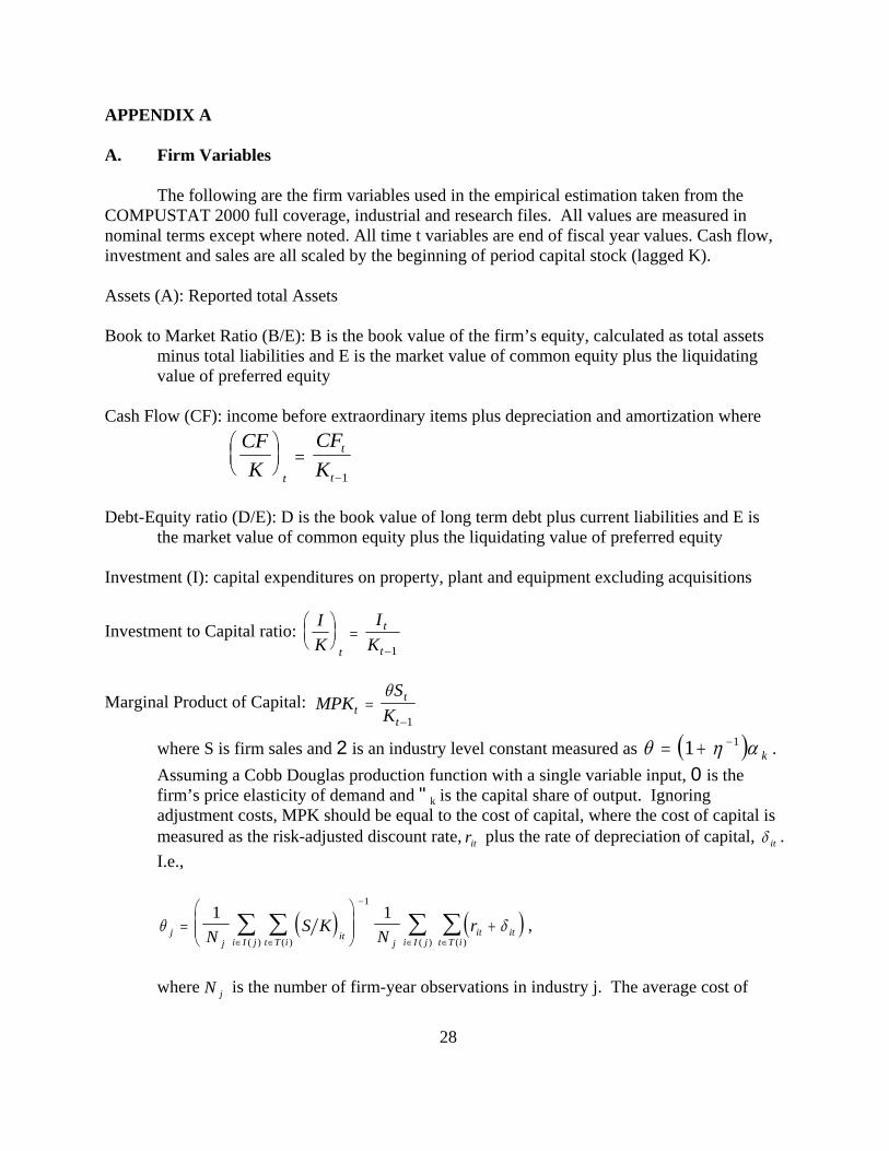
The following are the firm variables used in the empirical estimation taken from theCOMPUSTAT 2000 full coverage, industrial and research files. All values are measured innominal terms except where noted. All time t variables are end of fiscal year values. Cash flow,investment and sales are all scaled by the beginning of period capital stock (lagged K).

Assets (A): Reported total Assets

Book to Market Ratio (B/E): B is the book value of the firm’s equity, calculated as total assetsminus total liabilities and E is the market value of common equity plus the liquidating value of preferred equity

Cash Flow (CF): income before extraordinary items plus depreciation and amortization where

CFK

CFKt

t

t

⎛⎝⎜

⎞⎠⎟ =

−1

Debt-Equity ratio (D/E): D is the book value of long term debt plus current liabilities and E isthe market value of common equity plus the liquidating value of preferred equity

Investment (I): capital expenditures on property, plant and equipment excluding acquisitions

Investment to Capital ratio: IK

IKt

t

t

⎛⎝⎜

⎞⎠⎟ =

−1

Marginal Product of Capital: MPKS

Ktt

t=

−

θ

1

where S is firm sales and 2 is an industry level constant measured as . ( )θ η α= + −1 1k

Assuming a Cobb Douglas production function with a single variable input, 0 is thefirm’s price elasticity of demand and "k is the capital share of output. Ignoringadjustment costs, MPK should be equal to the cost of capital, where the cost of capital ismeasured as the risk-adjusted discount rate, plus the rate of depreciation of capital, . rit δ it

I.e.,

,( ) ( )θ δjj

itt T ii I j j i I jit it

t T iN S K N r=⎛

⎝⎜⎜

⎞

⎠⎟⎟ +

∈∈

−

∈ ∈∑∑ ∑ ∑1 1

1

( )( ) ( ) ( )

where is the number of firm-year observations in industry j. The average cost ofN j

29

capital is set equal to 0.18 . See Gilchrist and Himmelberg (1998) for further details.

Replacement value of the capital stock: K KP

PI

Lt tt

tt=

⎛⎝⎜

⎞⎠⎟ +

⎡

⎣⎢

⎤

⎦⎥ −

⎛⎝⎜

⎞⎠⎟−

−1

11

2

where Pt is the price deflator for non-residential fixed investment from NIPA (National Income and Product Accounts and L is the average of Lt, the useful life of capital goods which is calculated as:

LGK I

DEPRtt t

t

=+−1

where GK is reported gross property, plant and equipment and DEPR is capitaldepreciation. See Salinger and Summers (1983) for a detailed explanation of thisperpetual inventory method.

Tobin's q : qE TL

Att t

t=

+

where E is the market value of common equity plus the liquidating value of preferredequity, TL is the book value of total liabilities, and A is the firm’s reported total assets asmeasured in Gilchrist and Himmelberg (1998).

B. Volatility Variables

Total volatility: $ ( )σ ττ

iti

i it

t

tr r

i

= −=

∑1 2

1

Market Volatility: $ ( )σ ττ

Mti

M Mt

t

tr r

i

= −=

∑1 2

1

Industry Volatility: $ ( )σ ττ

Iti

I It

t

tr r

i

= −=

∑1 2

1

Firm-Specific Volatility: ,$ $σ εε ττ

iti

i

t

t

i

==

∑1 2

1

where J = 1, 2, ..., ti . ti is the number of trading days in year t, riJ is the daily return on firm i’sequity, rMJ is the daily market index return, rIJ is the daily industry index return of firm i’s three-digit SIC group that is orthogonal to the market return, giJ is the residual from equation (1). Allvolatility estimates are annualized.

Table A1: Standard Investment Regressions

Panel A: Variable (1) (2) (3) (4) (5)

Tobin's q 0.0389 0.0204 0.0256 0.0170 0.0109(6.04) (3.43) (3.79) (2.82) (1.85)

MPKt-1 1.0328 0.8781 0.8752(11.78) (8.62) (8.67)

(CF/K)t-1 0.0668 0.0305 0.0267(7.20) (2.96) (2.55)

D/(D+E) -0.0960-(5.30)

F(n,2722) 16.52 23.17 18.64 23.49 25.05p-value 0 0 0 0 0Root MSE 0.11884 0.11485 0.1153 0.11285 0.11223No. of Firms 2722 2722 2722 2722 2722No. of observations 19579 19579 19579 19579 19579

Panel B: Variable (1) (2) (3) (4) (5)

(I/K)t-1 0.2381 0.1700 0.2247 0.2193 0.2132(14.00) (6.65) (13.17) (8.72) (8.48)

Tobin's q 0.0318 0.0252 0.0208 0.0205 0.0154(5.57) (4.67) (3.55) (3.61) (2.82)

MPKt-1 0.4812 0.0403 0.0541(4.16) (0.31) (0.41)

(CF/K)t-1 0.0569 0.0555 0.0524(6.59) (5.44) (5.04)

D/(D+E)t-1 -0.0647-(4.31)

F(n,2721) 26.33 28.66 26.33 28.88 29.47p-value 0 0 0 0 0Root MSE 0.11308 0.10999 0.11047 0.11012 0.10957No. of Firms 2722 2722 2722 2722 2722No. of observations 19579 19579 19579 19579 19579

1) The dependent variable is I/K. 2) Estimation is by instrumental variables (2SLS). Instruments are the lagged values of all the right- hand side variables plus lagged Sales/K, lagged I/K, and year dummies.3) Robust standard errors are calculated that allow for correlation within firms. T-statistics are in parenthesis.4) n=33+number of regressors.

30

APPENDIX B

Table B1: Irreversibility Classification of Equipment or Structure Investments

Irreversible (Industry Specific) Reversible (Non-Industry Specific)

Metalworking machinery AutosSpecial industry machinery Communication equipmentAgricultural machinery, except tractors Computer printersCommercial warehouses Computer storage devicesConstruction machinery, except tractors Computer tape drivesConstruction tractors Computer terminalsElectrical transmission, distribution, Direct access storage devices and industrial apparatus General industrial, including materials handling, equipmentFarm related buildings and structures Household appliancesFarm tractors Household furnitureIndustrial buildings Internal combustion enginesOther nonfarm structures Mainframe computersOther nonresidential equipment Mobile structuresAircraft Other furnitureInstruments Other office equipmentOffice buildings Personal computersOther electrical equipment Photocopy and related equipmentOther fabricated metal products Steam enginesService industry machinery Trucks, buses, and truck trailers

1) The Fixed Reproducible Tangible Wealth Data produced by the Bureau of Economic Analysis reports capital expenditures of each

two digit SIC industry according to the above criteria. Industries are then classified as Irreversible or Reversible based on the

industry-specificity of these investments.

31

Table B2: Two Digit SIC Industry Irreversibility Ranking

SIC Industries Fraction of Irreversible Investments Index

20 Food and kindred products 0.568 721 Tobacco products 0.521 322 Textile mill products 0.811 1923 Apparel and other textile products 0.543 424 Lumber and wood products 0.639 1125 Furniture and fixtures 0.695 1626 Paper and allied products 0.554 627 Printing and publishing 0.692 1528 Chemicals and allied products 0.404 129 Petroleum and coal products 0.500 230 Rubber and miscellaneous plastics products 0.835 2031 Leather and leather products 0.663 1432 Stone, clay, and glass products 0.551 533 Primary metal industries 0.604 834 Fabricated metal products 0.748 1735 Industrial machinery and equipment 0.614 1036 Electronic and other electric equipment 0.610 937 Motor vehicles and equipment 0.764 1838 Instruments and related products 0.645 1239 Miscellaneous manufacturing industries 0.649 13

1)The fraction of irreversible capital expenditures (based on dollar amounts) is calculated for each industry according to Table B1. Industries are ranked according to this measure to generate an Irreversibility Index. The higher the index, the more irreversible is the industry.

32

33

BIBLIOGRAPHY

Abel, A. (1983). Optimal investment under uncertainty. American Economic Review, 73, 228-233.

________ , A. Dixit, J. Eberly and R. Pindyck, (1996). Options, the value of capital, andinvestment. Quarterly Journal of Economics, 111, 753-777.

, and J. Eberly, (1994). Optimal investment with costly reversibility. Review ofEconomic Studies, 63, 581-593.

Arellano, M. and O. Bover, (1995). Another look at the instrumental variable estimation of errorcomponent models. Journal of Econometrics, 68, 29-51.

Baldwin, C. (1982). Optimal sequential investment when capital is not readily reversible. Journalof Finance, 37, 763-782.

Bar-Ilan, A. and W. Strange, (1996). Investment lags. American Economic Review, 86, 610-622.

Bell, G. and J. Campa, (1997). Irreversible investment and volatile markets: A study of thechemical processing industry. Review of Economics and Statistics, 79, 79-87.

Berk, J., R. Green and V. Naik, (1999). Optimal investment, growth options, and security returns.Journal of Finance, 54, 1553-1607.

Bernanke, B. (1983). Irreversibility, uncertainty, and cyclical investment. Quarterly Journal ofEconomics, 98, 85-106.

Black, F. (1976). Studies of stock market volatility changes. Proceedings of the AmericanStatistical Association, Business and Economics Statistics Section, 177-181.

Bond, S. and J. Cummins, (2001). Noisy share prices and the q model of investment. Workingpaper, IFS.

Brennan, M. and E. Schwartz, (1985). Evaluating Natural Resource Investments. Journal ofBusiness, 58, 135-157.

Bulan, L., C. Mayer and T. Somerville (2003). Irreversible investment, real options andcompetition: Evidence from real estate development. Working paper,Wharton School.

Caballero, R. and R. Pindyck, (1996). Uncertainty, investment and industry evolution.International Economic Review, 37, 641-662.

34

Chakraborty, A., S. Shiekh and N. Subramanian, (2004). Performance incentives, performancepressure and executive turnover. Working paper, Brandeis University.

Christie, A. (1982). The stochastic behavior of stock variables: Value, leverage and interest rateeffects. Journal of Financial Economics, 10, 407-432.

Dixit, A. and R. Pindyck, (1994), Investment Under Uncertainty. Princeton, NJ: PrincetonUniversity Press.

Erickson, T. and T. Whited, (2000). Measurement error and the relationship between investmentand q. Journal of Political Economy, 108, 1027-1057.

Favero, C., M. Pesaran and S. Sharma, (1994). A duration model of irreversible oil investment:Theory and empirical evidence. Journal of Applied Econometrics, 9, 95-112 .

Fazzari, S., R.G. Hubbard and B. Petersen, (1988). Financing constraints and corporateinvestment. Brookings Papers on Economic Activity, 1, 141-195.

Federer, J. (1993). The impact of uncertainty on aggregate investment spending: An empiricalanalysis. Journal of Money, Credit and Banking, 25, 30-48.

Ghosal, V. and P. Loungani, (1996). Product market competition and the impact of priceuncertainty on investment: Some evidence from U.S. manufacturing industries. Journal ofIndustrial Economics, 44, 217-228.

, (2000). The differential impact of uncertainty on investment in small and largebusinesses. Review of Economics and Statistics, 82, 338-349.

Gilchrist, S. and C. Himmelberg, (1998). Investment, fundamentals and finance. Working Paper665, NBER.

Gomes, J. (2001). Financing investment. American Economic Review, 91, 1263-1285.

Graham, J. and C. Harvey, (2001). The theory and practice of corporate finance: Evidence fromthe field. Journal of Financial Economics, 60, 187-243.

35

Guiso, L. and G. Parigi, (1999). Investment and demand uncertainty. Quarterly Journal ofEconomics, 114, 185-227.

Hartman, R. (1972). The effects of price and cost uncertainty on investment. Journal of EconomicTheory, 5, 258-266.

Hayashi, F. (1982), Tobin’s marginal q and average a: A neoclassical interpretation.Econometrica, 50, 215-224.

.

Holland, A., S. Ott and T. Riddiough, (2000). The role of uncertainty in investment: Anexamination of competing investment models using commercial real estate data. Real EstateEconomics, 28, 33-64.

Hubbard, R. G. (1998). Capital market imperfections and investment. Journal of EconomicLiterature, 36, 193-225.

Huizinga, J. (1993). Inflation uncertainty, relative price uncertainty, and investment in U.S.manufacturing. Journal of Money, Credit and Banking, 25, 521-549.

Hurn, A. and R. Wright, (1994). Geology or economics? Testing models of irreversibleinvestment using north sea oil data. Economic Journal, 104, 363-371.

Kulatilaka, N. and E. Perotti, (1998). Strategic growth options. Management Science, 44,1021-1031

Lang, O. and R. Stulz, (1996). Leverage, investment, and firm growth. Journal of FinancialEconomics, 40, 3-29.

Leahy, J. and T. Whited, (1996). The effects of uncertainty on investment: Some stylized facts.Journal of Money, Credit and Banking, 28, 64-83.

Majd, S. and R. Pindyck, (1987). Time to build, option value and investment decisions. Journalof Financial Economics, 18, 7-27.

Mauer, D. and A. Triantis, (1994). Interactions of corporate financing and investment decisions:A dynamic framework. Journal of Finance, 49, 1253-1277.

and S. Ott, (2000). Agency costs, underinvestment and optimal capital structure:The effect of growth options to expand. In Project Flexibility, Agency and Competition, edited by

36

M. Brennan and L.Trigeorgis, Oxford: Oxford University Press, 151-179.

McDonald, R. (2000). Real options and rules of thumb in capital budgeting. In Project Flexibility, Agency and Competition, edited by M. Brennan and L.Trigeorgis, Oxford:Oxford University Press, 13-33.

McDonald, R. and D. Siegel, (1985). Investment and the valuation of firms when there is anoption to shut down. International Economic Review, 26, 331-349.

_ , (1986). The value of waiting to invest. Quarterly Journal of Economics, 101, 707-727.

Moel, A. and P. Tufano, (2002). When are real options exercised? An empirical study of mineclosings. Review of Financial Studies, 15, 35-64.

Myers, S. (1977). Determinants of corporate borrowing. Journal of Financial Economics, 5, 147-175.

Paddock, J., D. Siegel and J. Smith, (1988). Option valuation of claims on real assets: The case ofoffshore petroleum leases. Quarterly Journal of Economics, 103, 755-784.

Pindyck, R. (1988). Irreversible investment, capacity choice and the value of the firm. AmericanEconomic Review, 78, 969-985.

________, (1991). Irreversibility and the explanation of investment behavior. In StochasticModels and Option Values, edited by D. Lund and B. Oksendal, Amsterdam: North-Holland.

________, (1993). A note on competitive investment under uncertainty. American EconomicReview, 83, 273-277.

________, and A. Solimano, (1993). Economic stability and aggregate investment. NBERMacroeconomics Annual, 8, 259-303.

Quigg, L. (1993). Empirical testing of real option pricing models. Journal of Finance, 48, 621-640.

Salinger, M. and L. Summers, (1983). Tax reform and corporate investment: A microeconomicsimulation study. In Behavioral Simulation Methods in Tax Policy Analysis, edited by M.Feldstein, Chicago: University of Chicago Press, 247-286

Schwert, G.W. (1989). Why does stock market volatility change over time? Journal of Finance,44, 1115-1153.

37

The determinants of firms’ hedging policies. Journal of Financialand Quantitative Analysis, 20, 391-405.

Titman, S. (1985). Urban land prices under uncertainty. American Economic Review, 65, 505-514.

Trigeorgis, L. (1996). Real Options. Cambridge, MA: MIT Press.

Table 1a: Descriptive Statistics (1964-1999)

Variable Mean Std. Dev. Minimum Median Maximum

I/K 0.2333 0.2049 0.0135 0.1813 1.2982

Tobin's q 1.4716 0.9307 0.6077 1.1877 6.5162

MPK 0.1514 0.1498 0.0123 0.1091 1.0149

CF/K 0.3023 0.6770 -3.5076 0.2734 2.9051

Assets (real) 17.7545 51.4785 0.0397 2.2553 374.6321

D/(D+E) 0.2599 0.2134 0.0000 0.2193 0.8333

Total Uncertainty: σit 0.4395 0.2536 0.1439 0.3644 1.4591

Market Uncertainty (b): βitσMt 0.0899 0.0646 -0.0487 0.0799 0.2967

Firm-Specific Uncertainty (b): σεit 0.4245 0.2563 0.1327 0.3472 1.4530

Market Uncertainty (c): βitσMt 0.0899 0.0646 -0.0487 0.0799 0.2967

Industry Uncertainty: γitσIt 0.0605 0.0841 -0.0979 0.0404 0.3853

Firm-Specific Uncertainty (c): σεit 0.4036 0.2682 0.0184 0.3316 1.4490

Number of Firms 2901Number of Observations 29639

1) Market Uncertainty (b) and Firm-Specific Uncertainty (b) correspond to the market decomposition of firm returns.2) Market Uncertainty (c) and Firm-Specific Uncertainty (c) correspond to the orthogonal market and industry decomposition of firm returns.

38

Table 1b: Sample Correlations

Variable I/K Tobin's q MPK Cash Flow D/(D+E) σit βitσMt (b) σεit (b) βitσMt (c) γitσIt

I/K 1

Tobin's q 0.2302 1

MPK 0.4413 0.056 1

Cash Flow 0.2676 0.081 0.2979 1

D/(D+E) -0.251 -0.4675 -0.0495 -0.2134 1

σit 0.0707 -0.0365 0.1444 -0.2015 0.1687 1

βitσMt (b) 0.0621 0.0544 -0.0437 -0.0061 0.0575 0.0917 1

σεit (b) 0.0667 -0.0431 0.1499 -0.202 0.1681 0.997 0.025 1

βitσMt (c) 0.0621 0.0544 -0.0437 -0.0061 0.0575 0.0917 1 0.025 1

γitσIt -0.0398 0.0414 -0.0511 0.023 0.0568 -0.0874 0.2267 -0.1062 0.2267 1

σεit (c) 0.0689 -0.0531 0.1486 -0.1969 0.1568 0.9694 -0.0071 0.975 -0.0071 -0.2719

1) Tobin's q, MPK, cash flow and the debt-ratio are lagged values consistent with the empirical specification.

39

Table 2: Base Regressions

Variable (a) (b) (c) (a) (b) (c)

Tobin's q 0.0132 0.0120 0.0124(2.17) (1.99) (2.05)

MPKt-1 0.7771 0.8000 0.8071(7.31) (7.56) (7.51)

(CF/K)t-1 0.0326 0.0322 0.0322(3.29) (3.24) (3.20)

Total Uncertainty: σit -0.4752 -0.1939-(11.53) -(4.10)

Market Uncertainty: βitσMt 0.6150 0.6141 -0.0300 0.0130(4.14) (3.99) -(0.22) (0.09)

Industry Uncertainty: γitσIt -0.1441 -0.1784-(1.32) -(2.09)

Firm-Specific Uncertainty: σεit -0.5381 -0.5193 -0.1882 -0.1677-(11.77) -(11.48) -(3.72) -(3.38)

F(n,2721) 16.81 16.41 16.25 25.11 24.51 23.85p-value 0 0 0 0 0 0Root MSE 0.1248 0.1257 0.1256 0.1125 0.1125 0.1127No. of Firms 2722 2722 2722 2722 2722 2722No. of observations 19579 19579 19579 19579 19579 19579

1) The dependent variable is I/K. Model (a) uses total volatility, model (b) corresponds to the market decompostion of firm returns, and model (c) corresponds to the orthogonal market and industry decompostion of firm returns.2) Estimation is by instrumental variables (2SLS). Instruments are lagged values of all the right-hand side variables plus lagged Sales/K, lagged I/K, and year dummies. Firm fixed effects are eliminated according to Arellano and Bover (1995).3) Robust standard errors are calculated that allows for correlation within firms. T-statistics are in parenthesis4) n=33+number of regressors.

40

Table 3: MPK (Marginal Profitability of Capital) Regressions


Tobin's q 0.0017 0.0003 0.0004(0.65) (0.12) (0.14)

MPKt-1 0.3383 0.3319 0.3226(6.83) (6.65) (6.33)

(CF/K)t-1 0.0113 0.0090 0.0098(2.42) (1.90) (2.01)


Market Uncertainty: βitσMt 0.6008 0.5665 0.3682 0.3495(5.86) (5.45) (5.47) (5.02)

Industry Uncertainty: γitσIt 0.0077 -0.0003(0.10) -(0.01)


F(n,2721) 12.29 11.03 10.56 27.54 24.4 23.11p-value 0 0 0 0 0 0Root MSE 0.0582 0.0632 0.0632 0.0410 0.0439 0.0442No. of Firms 2722 2722 2722 2722 2722 2722No. of observations 19579 19579 19579 19579 19579 19579

1) The dependent variable is MPK. Model (a) uses total volatility, model (b) corresponds to the market decompostion of firm returns, and model (c) corresponds to the orthogonal market and industry decompostion of firm returns.2) Estimation is by instrumental variables (2SLS). Instruments are lagged values of all the right-hand side variables plus lagged Sales/K, lagged I/K, and year dummies. Firm fixed effects are eliminated according to Arellano and Bover (1995).3) Robust standard errors are calculated that allows for correlation within firms. T-statistics are in parenthesis4) n=33+number of regressors.

41

Table 4: Irreversible Investment RegressionsIrreversible Investments Reversible Investments


Tobin's q 0.0245 0.0247 0.0242 0.0027 0.0014 0.0013(2.56) (2.53) (2.49) (0.34) (0.18) (0.17)

MPKt-1 0.6960 0.7252 0.7208 0.8840 0.9040 0.9246(5.32) (5.61) (5.56) (4.93) (5.06) (4.91)

(CF/K)t-1 0.0377 0.0366 0.0359 0.0297 0.0300 0.0303(3.07) (2.99) (2.91) (1.82) (1.84) (1.82)


Market Uncertainty: βitσMt -0.0665 0.0865 -0.0997 -0.1137-(0.25) (0.32) -(0.60) -(0.68)



F(n,k) 16.7 16.28 15.76 11.93 11.65 11.34p-value 0 0 0 0 0 0Root MSE 0.1154 0.1156 0.1159 0.1108 0.1111 0.1114No. of Firms 1432 1432 1432 1376 1376 1376No. of observations 9362 9362 9362 10217 10217 10217

1) The sub-samples are created according to the degree of irreversibility of invested capital at the 2-digit SIC level. See Appendix B for more details.2) The dependent variable is I/K. Model (a) uses total volatility, model (b) corresponds to the market decompostion of firm returns, and model (c) corresponds to the orthogonal market and industry decompostion of firm returns.3) Estimation is by instrumental variables (2SLS). Instruments are lagged values of all the right-hand side variables plus lagged Sales/K, lagged I/K, and year dummies. Firm fixed effects are eliminated according to Arellano and Bover (1995).4) Robust standard errors are calculated that allows for correlation within firms. T-statistics are in parenthesis5) n=33+number of regressors.k=number of firms-1

42

Table 5: Industry Concentration Regressions

Less Competitive Firms More Competitive FirmsVariable (a) (b) (c) (a) (b) (c)

Tobin's q 0.0178 0.0161 0.0158 0.0142 0.0138 0.0140(1.79) (1.65) (1.63) (1.63) (1.59) (1.60)

MPKt-1 0.4744 0.4915 0.4965 1.0511 1.0569 1.0727(3.31) (3.43) (3.45) (4.49) (4.52) (4.64)

(CF/K)t-1 0.0459 0.0445 0.0455 0.0238 0.0231 0.0221(3.14) (2.99) (3.05) (0.75) (0.74) (0.70)


Market Uncertainty: βitσMt -0.0145 0.0897 0.0888 0.1068-(0.07) (0.42) (0.45) (0.54)




1) The sub-samples are created according to the degree of competitiveness of the firm in a four digit SIC industry as measured by industry concentration ratios from the 1992 Census of Manufactures.2) The dependent variable is I/K. Model (a) uses total volatility, model (b) corresponds to the market decompostion of firm returns, and model (c) corresponds to the orthogonal market and industry decompostion of firm returns.3) Estimation is by instrumental variables (2SLS). Instruments are lagged values of all the right-hand side variables plus lagged Sales/K, lagged I/K, and year dummies. Firm fixed effects are eliminated according to Arellano and Bover (1995).4) Robust standard errors are calculated that allows for correlation within firms. T-statistics are in parenthesis

43

Table 6: Size Regressions Based on Real Total Assets

Large Firms Small FirmsVariable (a) (b) (c) (a) (b) (c)

Tobin's q 0.0219 0.0216 0.0219 0.0056 0.0055 0.0055(3.45) (3.41) (3.47) (0.43) (0.42) (0.43)

MPKt-1 0.8812 0.8892 0.8904 0.6757 0.6743 0.6656(6.91) (6.92) (7.00) (4.98) (4.99) (4.84)

(CF/K)t-1 0.0398 0.0384 0.0402 0.0300 0.0329 0.0333(2.79) (2.68) (2.78) (2.63) (2.76) (2.79)


Market Uncertainty: βitσMt 0.0681 0.1284 -0.4257 -0.4007(0.59) (1.07) -(0.83) -(0.76)




1) The full sampe is divided at the median average-firm size measured by total real assets.2) The dependent variable is I/K. Model (a) uses total volatility, model (b) corresponds to the market decompostion of firm returns, and model (c) corresponds to the orthogonal market and industry decompostion of firm returns.3) Estimation is by instrumental variables (2SLS). Instruments are lagged values of all the right-hand side variables plus lagged Sales/K, lagged I/K, and year dummies. Firm fixed effects are eliminated according to Arellano and Bover (1995).4) Robust standard errors are calculated that allows for correlation within firms. T-statistics are in parenthesis

44

Table 7: Leverage

Unlevered Volatility Levered Volatility Unlevered Firms

Variable (a) (b) (c) (a) (b) (c) (a) (b) (c)

Tobin's q 0.0103 0.0090 0.0091 0.0065 0.0046 0.0053 0.0114 0.0099 0.0105(1.76) (1.56) (1.57) (1.08) (0.76) (0.87) (1.15) (0.98) (1.06)

MPKt-1 0.7958 0.8200 0.8294 0.7222 0.7643 0.7760 0.7532 0.7763 0.7919(7.54) (7.82) (7.79) (6.90) (7.39) (7.30) (4.22) (4.48) (4.43)

(CF/K)t-1 0.0298 0.0294 0.0289 0.0335 0.0319 0.0315 0.0259 0.0271 0.0254(2.91) (2.88) (2.79) (3.33) (3.19) (3.06) (1.72) (1.78) (1.64)

D/(D+E)t-1 -0.0600 -0.0642 -0.0715 -0.1724 -0.1659 -0.1655-(2.70) -(2.83) -(3.12) -(7.11) -(6.55) -(6.57)

Total Uncertainty : σit -0.1542 -0.3660 -0.3710-(2.95) -(4.17) -(2.26)

Market Uncertainty : βitσMt -0.0569 -0.0088 0.0074 0.0760 -0.2724 -0.1479-(0.41) -(0.06) (0.04) (0.38) -(0.79) -(0.41)

Industry Uncertainty : γitσIt -0.1826 -0.3590 -0.4330-(2.13) -(2.80) -(1.73)

Firm-Specific Uncertainty : σεit -0.1421 -0.1173 -0.3395 -0.2885 -0.3522 -0.3053-(2.52) -(2.11) -(3.56) -(3.09) -(2.02) -(1.75)

F(n,k) 25.83 25.29 24.64 25.65 24.5 24.66 6.24 6.16 5.93p-value 0 0 0 0 0 0 0 0 0Root MSE 0.1119 0.1121 0.1124 0.1130 0.1124 0.1127 0.1473 0.1481 0.1488No. of Firms 2722 2722 2722 2722 2722 2722 898 898 898No. of observations 19579 19579 19579 19579 19579 19579 5318 5318 5318

1) The dependent variable is I/K. Model (a) uses total volatility, model (b) corresponds to the market decompostion of firm returns, and model (c) corresponds to the orthogonal market and industry decompostion of firm returns.2) Unlevered volatility measures are calculated by multiplying volatility by E/(D+E). The sub-sample of unlevered firms is the bottom third (33rd percentile) of firms in terms of leverage with a mean leverage ratio of 4.3 %.3) Estimation is by instrumental variables (2SLS). Instruments are lagged values of all the right-hand side variables plus lagged Sales/K, lagged I/K, and year dummies.4) Robust standard errors are calculated that allows for correlation within firms. T-statistics are in parenthesis5) n=33+number of regressors.k=number of firms-1

45

Real Options, Irreversible Investment and Firm Uncertainty...

Documents

Transcript of Real Options, Irreversible Investment and Firm Uncertainty...