Real Estate Valuation, Current Account and Credit …Real Estate Valuation, Current Account and...

NBER WORKING PAPER SERIES

REAL ESTATE VALUATION, CURRENT ACCOUNT AND CREDIT GROWTHPATTERNS, BEFORE AND AFTER THE 2008-9 CRISIS

Joshua AizenmanYothin Jinjarak

Working Paper 19190http://www.nber.org/papers/w19190

NATIONAL BUREAU OF ECONOMIC RESEARCH1050 Massachusetts Avenue

Cambridge, MA 02138June 2013

The views expressed herein are those of the authors and do not necessarily reflect the views of theNational Bureau of Economic Research. We thank Livio Stracca and the participants at the conferenceon "Current Account Imbalances and International Financial Integration," hosted by the EuropeanCommission in Brussels, 6-7 December 2013, as well as the seminar at Victoria University of Wellington,for useful comments and suggestions.

NBER working papers are circulated for discussion and comment purposes. They have not been peer-reviewed or been subject to the review by the NBER Board of Directors that accompanies officialNBER publications.

© 2013 by Joshua Aizenman and Yothin Jinjarak. All rights reserved. Short sections of text, not toexceed two paragraphs, may be quoted without explicit permission provided that full credit, including© notice, is given to the source.

Real Estate Valuation, Current Account and Credit Growth Patterns, Before and After the2008-9 CrisisJoshua Aizenman and Yothin JinjarakNBER Working Paper No. 19190June 2013, Revised March 2014JEL No. F15,F21,F32,R21,R31

ABSTRACT

We explore the stability of the conditioning variables accounting for the real estate valuation beforeand after the crisis of 2008-9, in a panel of 36 countries, recognizing the crisis break. We validate therobustness of the association between the real estate valuation and lagged current account patterns,both before and after the crisis. The most economically significant variable in accounting for real estatevaluation changes turned out to be the lagged real estate valuation appreciation (real estate inflationminus CPI inflation), followed by lagged declines of the current account/GDP, lagged domestic credit/GDPgrowth, and lagged equity market valuation appreciation (equity market appreciation minus CPI inflation).A one standard deviation increase in lagged real estate appreciation is associated with a 10 % increasein the present real estate appreciation, larger than the impact of a one standard deviation deteriorationin the lagged current account/GDP (5%) and of the lagged domestic credit/GDP growth (3%). Theresults are supportive of both current account and credit growth channels, with the momentum channelsplaying the most important role. Smaller current account/GDP surpluses or larger deficits may serveas warning signals, especially when coinciding with credit expansion and real estate appreciation duringthe past several quarters.

Joshua AizenmanEconomics and SIRUSCUniversity ParkLos Angeles, CA 90089-0043and [email protected]

Yothin JinjarakDeFiMS SOASUniversity of London, United Kingdomand ADB Institute, [email protected]

2

1. Introduction and overview

The global crisis of 2008-9 sparked a vibrant debate on the factors contributing to the

crisis. Were global imbalances or excessive credit growth the key suspects? Contributors to the

debate include Borio and Disyatat (2011), conjecturing that the main causing factor to the

financial crisis was not “excess saving” but the “excess elasticity” of the international monetary

and financial system; and Obstfeld (2012:20), noting that “The balance sheet mismatches of

leveraged entities provide the most direct indicators of potential instability, much more so than

do global imbalances, though the imbalances may well be a symptom that deeper financial

threats are gathering.” Against this background, we revisit these questions in the context of the

real estate market. The macro importance of the real estate market is well appreciated by now.

A prime example of it has been the U.S., where Leamer (2007)’s title succinctly summarized it:

“Housing is the business cycle.”

A priori, one expects that both the current account and credit growth trends would impact

the valuation of national real estates. A primary link between real estate valuation and the

current account deficit follows from national accounting and the absorption approach. Growing

current account deficits is a signal of a growing gap between the spending of domestic residents

[absorption] and their output. As long as the demand for key non-traded durable assets, like real

estate, is positively correlated with absorption, one expects higher current account deficits to be

associated with higher real estate valuation. Yet, as most households co-finance the purchase of

their dwelling through the banking system, greater financial depth and accelerated growth rate of

credit tend to increase the demand for houses, probably increasing the real estate valuation.

Thus, one expects that both current account and credit trends matter for the valuation of

real estate, and a priori there is no obvious reason to surmise which of the two should dominate.

In Aizenman and Jinjarak (2009) we looked empirically at these issues in 41 countries, for the

years 1990–2005, investigating the association between lagged current account deteriorations

and the appreciation of the real estate prices/GDP deflator, controlling for macro factors

associated with real estate valuation [lagged GDP/capita growth, inflation, financial depth,

institution, urban population growth and the real interest rate]. We found a strong positive

association between lagged current account deteriorations and an appreciation of the real estate,

where the real appreciation is magnified by financial depth, and mitigated by the quality of

3

institutions. Intriguingly, the economic importance of current account variations, in accounting

for the real estate valuation, exceeds that of the other variables, including the real interest rate

and inflation.

A growing literature identified several related channels contributing to the positive

association of the current account and credit growth patterns with real estate valuation. Tomura

(2010) analyzed the roles of credit market conditions in the endogenous formation of housing-

market boom–bust cycles, in a business cycle model. When households are uncertain about the

duration of a temporary high income growth period, expected future house prices rise during a

high growth period and fall at the end of the period. These developments induce in his model

expectation-driven boom–bust cycles in house prices, only if the economy is open to

international capital flows. Furthermore, high maximum loan-to-value ratios for residential

mortgages per se do not cause boom–bust cycles without international capital flows. Laibson

and Mollerstrom (2010) noted that national asset bubbles may explain the international

imbalances -- the bubbles raised consumption, resulting in large trade deficits. In their sample of

18 OECD countries plus China, movements in home prices alone explain half of the variation in

trade deficits. Gete’s (2010) model showed that an increased demand for housing may generate

trade deficits without the need for wealth effects or trade in capital goods, and that housing

booms are larger if the country can run a trade deficit. These predictions were found consistent

with the pre-crisis experience of the OECD countries. Adam et al. (2011) outlined an open

economy asset pricing model with households characterized by subjective beliefs about price

behavior and update these beliefs using Bayes' rule. They show that the resulting belief dynamics

propagate considerable economic shocks and contribute to replicating the empirical evidence of

the association between current account patterns and real estate valuations. Belief dynamics can

temporarily delink house prices from fundamentals, so that low interest rates can fuel a house

price boom.

As there is no reason for the relative importance of the current account and the credit

patterns to stay stable overtime in accounting real estate valuation, we explore in this paper the

degree to which the pre global crisis patterns continues to hold after the crisis. Specifically, we

look at the following questions:

4

i. Stability of the key conditioning variables accounting for the real estate valuation before

and after the crisis; specifically the relative importance of the current account and credit

growth patterns.

ii. The importance of ‘momentum’ in the pricing of real estate, as measured by the impact of

lagged real estate appreciation in accounting for the present real estate appreciation,

controlling for other macro factors. This issue is related to concerns about possible

bubble dynamics, where lagged appreciation is reinforcing expectations of future

appreciation.

iii. Symmetry of the patterns during real estate appreciation versus real estate depreciation.

iv. The possible two way causality between current account and real estate valuation

patterns.

v. The degree to which the valuation of equities is accented by similar conditioning

variables.

Overall, our paper reveals a complex of time varying patterns, yet it validates the

robustness of the association between real estate valuation of lagged current account patterns

both before and after the crisis. The base regression is a dynamic panel estimate of 36 countries,

during the periods 2005:I -2012:IV, recognizing the crisis break. It accounts for the appreciation

rate of the real estate valuation (real estate inflation minus CPI inflation) as explained by the

following correlates: lagged appreciation rate of the real estate valuation, lagged decline in the

current account/GDP, lagged changes in the domestic credit/GDP, lagged changes in the equity

market valuation appreciation (equity market appreciation minus CPI inflation), and a vector of

lagged changes of macro controls [inflation, growth of industrial production, TED spreads,

sovereign spreads, VIX, and international reserves]. The most economically significant variable

in accounting for real estate valuation changes turned out to be the lagged real estate valuation

appreciation, followed by lagged declines of the current account/GDP, lagged domestic

credit/GDP growth, and lagged equity market valuation appreciation. The first three effects are

economically substantial: a one standard deviation increase in lagged real estate appreciation is

associated with a 10 % increase in the present real estate appreciation, much larger than the

impact of a one standard deviation decline in the lagged current account (5%), and that of lagged

increase in the domestic credit/GDP growth (3%). Thus, the results are supportive of both current

5

account and credit growth channels, with the animal-spirits and expectations channels playing

the most important role in the boom and bust of real estate valuation.

While positive reverse feedback of real estate appreciation to current account

deteriorations cannot be ruled out theoretically, we find that it is not supported during our sample

period. We find support for a positive feedback of real estate appreciation to equity market

appreciation, which is consistent with the wealth effects from real estate valuation to equity

investment.

2. Sample

We use quarterly data to understand how short- to medium-term adjustment of the real

estate valuation interacts with current accounts, domestic credit, and relevant macro and global

variables. Using quarterly data comes at a cost of sample length: subject to data availability, our

data covers the period of 2005:I to 2012:IV. Obviously we miss out earlier episodes of real

estate booms and busts. However, in the present context of our investigation this may not be so

costly since previous cycles would be varying across countries, meaning that there would be a

variety of other driving factors in country-specific episodes. On the other hand, the current

sample period fits well with our interests that specifically focus on the real estate valuation over

the global crisis, with quarterly adjustment dynamics. Alternatively, using annual data instead

would allow for a longer sample period back in the historical past, but could not capture the

dynamics of short- to medium-term interactions between real estate data and confounding macro

fundamentals that we try to understand.

The data are drawn from several sources, as shown in Appendix A, including Oxford

Economics, Economist Intelligence Unit (EIU), Federal Reserve Economic Data (FRED), and

Credit Market Analysis (CMA). Our main variable of interests is real estate valuation

appreciation (real estate inflation minus CPI inflation). As a user of secondary data, we are made

well aware that the primary collection method of our most important variable, the real estate

valuation series, is known to be highly heterogeneous across countries. National statistical

offices and local real estate agencies have their own approaches in compiling the data; e.g. some

are repeated sales, others are not; some include both residential and commercial, others do not,

etc. Hence, pooling real estate series across countries amounts to an aggregation problem. Our

6

real estate series, which are drawn from a compilation of Oxford Economics database, are also

subject to this data issue, as is the case in other earlier studies and datasets.1 Yet, as is shown in

Aizenman and Jinjarak (2009) using real estate data from different cross-country databases,

residential series and commercial real estate series, the econometric evidence are largely

consistent across the data sets on the empirical relationships of real estate, current account, and

macro variables.

Altogether there are 36 countries in the sample, covering both developed and emerging

markets. Appendix A provides the list of countries and Appendix B shows geographically the

locality of real estate markets included. Some of these are large, hot spot markets, widely

monitored and publicized by the press, e.g. China and the US, whereas many others are smaller

in size and may not be known as boom-bust spots in the global real estate markets. As shown by

standard deviation of real estate valuation appreciation highlighted in the figure of Appendix B,

several of these countries are considered highly volatile markets for the period before and after

the global crisis.

2.1 Preliminary statistics

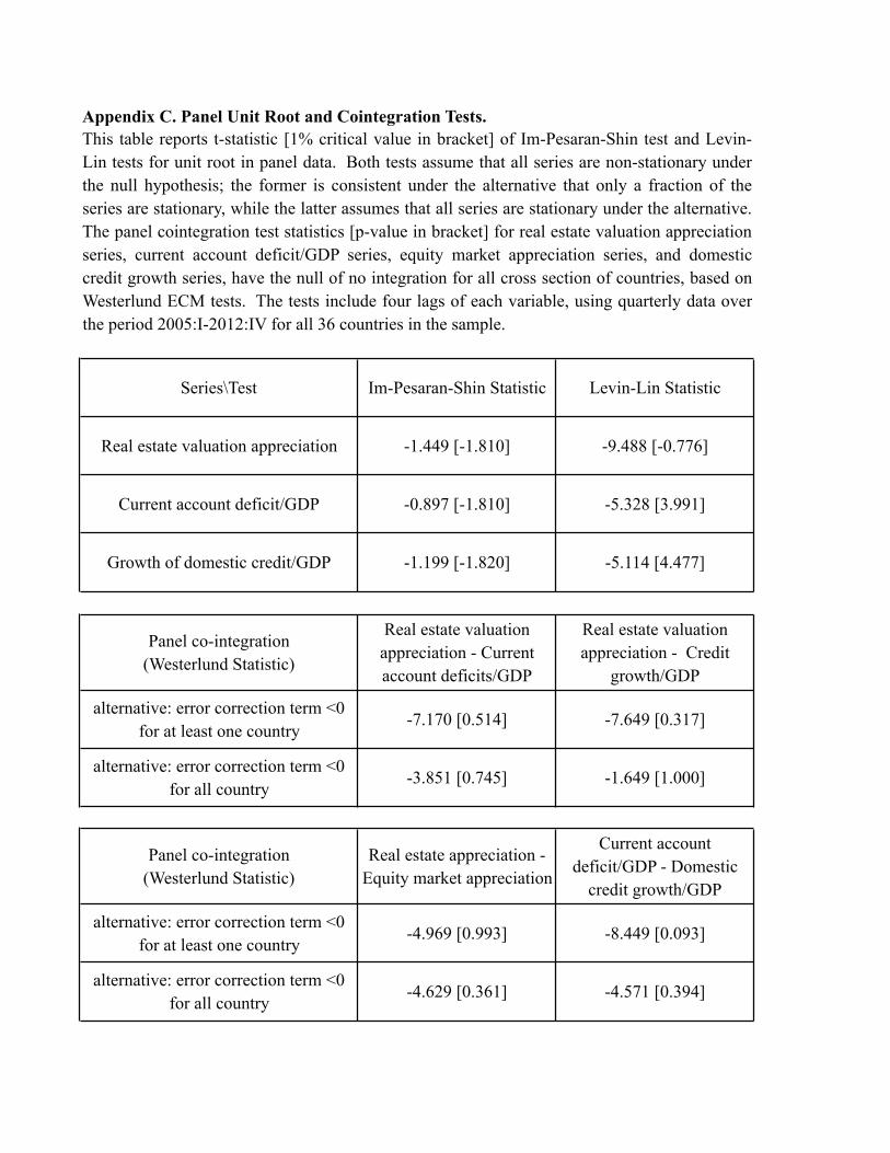
Panel unit root tests suggest that real estate valuation appreciation, current account/GDP

deterioration, and domestic credit growth/GDP are all nonstationary. As the power of unit root

tests undoubtedly varies across study samples, not to mention panel data extension of the tests,

we report both Im-Pesaran-Shin statistic and Levin-Lin statistic (Appendix C). These two tests

assume that all series are non-stationary under the null hypothesis; the former is consistent under

the alternative that only a fraction of the series are stationary, while the latter assumes that all

series are stationary under the alternative. Both tests appear consistent with each other in our

sample, pointing to the existence of unit roots in the series. Next, we examine whether there is

any co-integrating relationship among these variables.2

1 The cross-country series currently available are not sufficiently detailed to resolve the issues, as well as in term of

cross-series comparability, in contrast to, for example, Standard and Poor’s (S&P) Case-Shiller for the US real estate

series.2 To smooth seasonal fluctuations in quarterly real estate valuation appreciation, current account/GDP deterioration, and domestic credit growth/GDP, we use their four-quarter moving averages (current plus three lags) here and in the following estimation.

7

The panel co-integration test does not reject the null of no co-integration between real

estate valuation appreciation and current account/GDP deterioration; real estate valuation

appreciation and domestic credit growth/GDP; real estate valuation appreciation and equity

market valuation appreciation (equity market appreciation minus CPI inflation); current account

/GDP deterioration and domestic credit growth/GDP. The panel co-integration test statistics

have the null of no integration for all cross-sections of countries, based on Westerlund panel

error-correction-model (ECM) tests. We report test statistics both when an alternative is error

correction term less than zero for at least one country, and when an alternative is error correction

term less than zero for all countries. Both statistics are consistent with each other in rejecting co-

integration. While there is some weak evidence of co-integration between current account/GDP

deterioration and domestic credit growth/GDP, this is not statistically significant at the 5 percent

level of the test.

Based on the panel unit-root and panel co-integration tests, the application of dynamic

panel data estimation in first-differenced series is deemed necessary for the real estate and macro

variables in our sample. With 36 countries and over 20 quarterly periods for each country, the

fixed-effect estimation may also be applicable. However, given that several series are known to

be highly persistent in the panel of countries (i.e. real estate prices, current accounts, domestic

credit growth, as well as equity prices), including lagged terms of dependent variables on the

right-hand side of estimating equations may entail empirical correlation between the lagged

regressors and the error terms, and hence the endogeneity issue. For these reasons, we focus in

the following on coefficient estimates from dynamic panel estimation as our main econometric

evidence.

2.2 Patterns of real estate valuation appreciation and current account/GDP deterioration

Mean reversion in real estate appreciation across national markets is quite noticeable in

the data. As shown in Figure 1, we plot cumulative real estate valuation appreciation for the

period of 2005:I-2007:III on the horizontal axis, and cumulative real estate valuation

appreciation for the period of 2008:III-2012:IV on the vertical axis. The relationship between

cumulative real estate appreciation between the two periods is negative: the slope coefficient

from OLS estimation is -0.5 and is statistically significant at the 1 percent level, with R2 = 0.28.

Ireland, Spain, South Africa, United States, and United Kingdom provide clear example of mean

8

revision before and after the global crisis. There are a few outliers in this relationship; including

mostly small markets, i.e. Hong Kong, Ireland, and Romania (not included in the plot for

illustrative purposes).

Once we plot the country-specific evolution of real estate valuation appreciation series, it

appears that there are large differences across countries in the associated patterns against the

backdrop of the global financial crisis. Shown in Figure 2A, real estate valuation varied

markedly before and after the global crisis events, as marked by the two vertical lines for

2007:III (Northern Rock event) and for 2008:III (Lehman Brother event), respectively. While

real estate valuation appreciation of some countries increased until the crisis events (e.g. Canada,

Ireland), for several others the real estate valuation appreciation valuation were already spiraling

downward even before the global crisis (e.g. US, South Africa). For some markets, the real

estate valuation appreciation appear to bounce back soon after the global financial panic (e.g.

Australia), while for a few others, national real estate markets continued to be highly volatile

(e.g. Hong Kong, Singapore).

The patterns of current account/GDP deterioration and domestic credit growth/GDP were

also heterogeneous across countries over the periods before and after the global financial crisis.

As shown in Figure 2A for current account/GDP deterioration and in Figure 2B for domestic

credit growth/GDP, the quarterly adjustment dynamics of these two variables tracked real estate

valuation appreciation in some countries quite well, whereas for several others there appeared no

relationship between the two variables and the real estate valuation appreciation valuation.

Hence, as an alternative to using the global crisis events (i.e. Northern Rock even and Lehman

Brothers event) to mark the turning points, we assign a new binary variable "Current

account/GDP's deterioration Break" to identify a country-specific break date, or structural shift,

in the empirical association between real estate valuation appreciation and current account/GDP

deterioration, according to QLR statistics3; and a new binary variable "Domestic credit/GDP's

Break", which is defined similarly for the stock of domestic credit/GDP. As shown in figures 2A

3 Quandt likelihood ratio test for a break at an unknown break date (Stock and Watson, 2012). Here we are mainly

interested in empirical breaks of the association between real estate valuation appreciation and current account/GDP

deterioration (or growth of domestic credit/GDP) in each country over the sample period of 2005:I-2012:IV. For

identification of extreme capital flow episodes from 1986-2009, see Forbes and Warnock (2012).

9

and 2B, these empirical turning points closely resemble the global crisis events for a majority of

countries (notably, i.e. US, UK, Australia, Spain), whereas they were not the same turning points

in a number of countries.

3. Baseline Results

3.1 The Global Financial Crisis

From our baseline estimation, real estate valuation is positively and significantly

associated with current account deficits in both periods before and after the crisis of 2008-09.

Real estate valuation is positively associated with domestic credit growth to a lesser degree,

statistically significant only in the period before the crisis [see Appendix D for the empirical

specification]. Column 1 of Table 1 provides the main results, using 2007:III (Northern Rock

event) as the turning point that marked the global financial crisis, while column 2 uses 2008:III

(Lehman Brothers event) as an alternative turning point. Both estimation results are consistent

with each other, suggesting that the association of real estate valuation appreciation with current

account/GDP deterioration and with domestic credit growth/GDP are positive and statistically

significant (accounting coefficient estimates on the four lags of current account deficit and

domestic credit growth).4

The baseline results also show that equity market appreciation and inflation are

empirically associated with real estate valuation, while the relationship with other variables

(growth, global interest rate, sovereign risk, reserve accumulation) is not supported in the current

sample. The positive association between real estate valuation appreciation and equity market

valuation appreciation is consistent with the wealth effects from real estate valuation to equity

investment, as capital gains in the equity investment spillover to the real estate sector. The

association between real estate valuation appreciation and inflation is negative as one might

expect. The coefficients of other variables are not statistically significant; for some variables,

coefficient estimates have an unexpected sign (i.e. growth of industrial production, TED spread,

and foreign reserve accumulation).

4 The coefficients are obtained from the Arellano-Bond dynamic panel estimation. While only lagged real estate

valuation appreciation is treated as an endogenous regressor, the autocorrelation test suggests that AR(2) is only

marginally significant at the 10 percent level, but not at the 5 percent level.

10

Interestingly, coefficient estimates of lagged real estate valuation appreciation indicate

persistence in real estate valuation up to two quarters, consistent with popular commentaries that

real estate markets are driven by animal spirits and momentum, with macroeconomic and

regulatory environment playing a supporting role. The lagged real estate coefficients are equal

to 0.6 for the first two quarters and statistically significant at the 1 percent level, suggesting that

more than half of real estate valuation was carried on from one quarter to the next three quarters

on average.5 However, our sample focuses on a specific episode before and after the global

crisis. Hence, the findings do not imply that expectation-driven persistence in real estate

valuation may last only half a year, but instead that this observed momentum appears to be the

case over the period of 2005:I to 2012:IV.

3.2 Breaks in current account deficits and domestic credit growth

The positive association between real estate appreciation and current account

deterioration remains robust for alternative turning points in their relationship, but the

association between real estate appreciation and domestic credit growth does not. As shown

earlier in Figures 2A and 2B, for a majority of countries, the global crisis events (Northern Rock

in 2007:III and Lehman Brothers in 2008:III) coincided with the empirical turning points in the

relationship between real estate valuation appreciation and current account/GDP deterioration, as

well as the relationship between real estate valuation appreciation and domestic credit

growth/GDP. To verify, instead of using a Global crisis binary variable as done in Table 1, we

use in Table 2 a new binary variable "Current account/GDP deterioration's Break" that identifies

a country-specific turning point in the association between real estate appreciation and current

account/GDP deterioration, according to QLR statistics as described in Section 2.2; "Growth of

domestic credit/GDP's Break" is defined similarly for domestic credit growth/GDP; both are

depicted in Figure 2. These country-specific breaks enter the estimation of Table 2 individually,

and also as interaction terms with current account deficit/GDP series and with growth of

domestic credit/GDP series. Table 2 column 1 reports the dynamic panel estimates from these

new specifications. We find that the positive association between real estate valuation

appreciation and current account/GDP deterioration is still statistically significant, while the

5 The coefficient estimate on a third lag is negative, but much smaller than the first two, so the net effect remains positive for three quarters. In Section 4, we revisit the economic significance of lagged real estate valuation in more details.

11

positive association between real estate valuation appreciation and growth of domestic

credit/GDP becomes insignificant.

In addition, with these alternative turning points, using the fixed-effect estimation does

not change the main finding on the positive and statistically significant association between real

estate valuation and current account deficit. As shown in column 2 of Table 2, the coefficient

estimates of current account/GDP deterioration remain statistically significant in the fixed-effect

estimation; the coefficient estimates of lagged real estate valuation appreciation and equity

market valuation appreciation also remain statistically significant. Further, current account

deficit/GDP enters the estimation positive and statistically significant both individually and as

interaction terms. The explanatory power, as measured by R2 in column 2, suggests that the

estimation is able to explain about 80 percent of variation in the real estate valuation over the

period of 2005:I to 2012:IV. Since a drawback of fixed-effect estimation is a lack of empirical

treatment on endogeneity in the presence of lagged dependent variable (real estate valuation

appreciation), we take the fixed-effect estimates as supportive evidence and continue onwards

with the dynamic panel estimation in the following.6

3.3 Current account deterioration vis-à-vis of domestic credit growth

Horseracing lagged current account/GDP changes vis-à-vis lagged growth of domestic

credit/GDP suggests that the former is more statistically significant in the empirical association

with real estate valuation changes. The findings in Tables 1 and 2 indicates that the positive

association between real estate valuation appreciation and lagged current account /GDP declines

is always statistically significant, whereas the association between real estate valuation

appreciation and lagged growth of domestic credit/GDP is insignificant in several specifications

(i.e. columns 1 and 2 of Table 2). Perhaps this difference might be due to common underlying

6 For real estate valuation and current account relationship, it is beyond a scope of the study to defend either method

of the panel estimation. Hypothetically, in the context of reduced-form analysis, endogenous regressors may include

not only lagged real estate valuation appreciation, but also additional lags of the right-hand-side variables, i.e.

current account/GDP deterioration, growth of domestic credit/GDP, and equity market valuation appreciation.

Alternatively, one may consider current account as endogenous and study the present value of current account with

real estate valuation (and for that matter, other asset prices) and VAR (although the causal ordering has never been

clear in such setting for all contemporaneous coordinates). Essentially, in the general-equilibrium analysis, all the

variables would be endogenous, even the incidence of global crises. Hence, since we take no stance and there is no

point to be too defensive about the main specifications reported in this paper, instead we hereby provide a battery of

results based on various specifications for the readers to judge.

12

factors in both current account and credit growth series; the patterns illustrated in Figures 2A and

2B seem to suggest that both series tracked real estate valuation appreciation quite well for a

majority of countries, before and after the global crisis. Alternatively, the difference might be

due to insufficient lagged adjustment allowed for these two variables in the estimation.

Accordingly, in Table 3 we allow for four lags of current account/GDP deterioration in column

1, excluding growth of domestic credit/GDP and a binary variable for global crisis or a binary

variable for turning points in the association between real estate valuation appreciation and

current account/GDP deterioration. Similarly, we allow for four lags of growth of domestic

credit/GDP in column 2, excluding current account /GDP declines and a binary variable for

global crisis or for the turning points in growth of domestic credit/GDP. Based on these

alternative specifications, the findings are consistent with the coefficient estimates of Tables 1

and 2. Without growth of domestic credit/GDP in the estimation, the association between real

estate valuation appreciation and current account/GDP deterioration remains positive and

significant (column 1). On the other hand, without current account/GDP deterioration in the

estimation, the association between real estate valuation appreciation and growth of domestic

credit/GDP is still weak and insignificant at all lags (column 2).

Based on statistical pair-wise correlation and panel co-integration tests, multi-collinearity

between current account deterioration and growth of domestic credit is unlikely, at least for the

2005:I-2012:IV sample. As discussed earlier via Appendix C, the panel co-integration tests

cannot reject the null of no co-integration between current account/GDP declines and growth of

domestic credit/GDP. We also find that the pair-wise correlation between the two series is only

0.1 across countries in our sample. Nevertheless, this does not imply that we should rule out

altogether potential feedback between current account deficit changes and growth of domestic

credit in other samples, presumably with a longer sample and covering episodes other than we

currently examine. Useful extension may also try to understand causality between current

account changes and credit growth across time and countries. One may suspect some

intertwining of household debt accumulation, consumption of durables, and domestic

indebtedness in foreign currency become important factors in such setting.

13

4. Sensitivity Analysis

4.1 Reverse feedback

We find that reverse and positive feedback of real estate appreciation to current account

deterioration is not supported by the data over the crisis period. To investigate for possible

feedback from real estate valuation appreciation, Table 4 column 1 reverses the empirical

specification of column 1 in Table 1 by placing current account/GDP declines on the left-hand

side of the estimating equation. This specification is not a straightjacket model of current

account, but is a simple verification of possible influence on current account from real estate

valuation. The coefficient estimates suggest that there is no evidence of positive feedback of real

estate valuation appreciation to current account/GDP declines in the data. As shown in Table 4,

the coefficient estimates of real estate valuation appreciation, while statistically significant, have

negative sign, opposite to what one might expect, before and after the global crisis period. This

counterintuitive finding seems to be rather consistent with the panel co-integration tests in

Appendix C where we cannot reject the null of no co-integration between current account/GDP

deterioration and real estate valuation appreciation. However, these non-findings do not rule out

positive and reverse feedback of real estate appreciation to current account deteriorations in other

samples, but only that any support for such reverse feedback is not prevalent during 2005:I-

2012:IV period that we study.

On the other hand, and contrary to panel co-integration tests, the coefficient estimates of

dynamic panel estimation suggest positive feedback of real estate appreciation to equity market

appreciation, a finding consistent with the wealth effects from real estate valuation to equity

investment. In column 2 of Table 4, we replace a left-hand-side variable of the estimating

equation with equity market valuation appreciation. As shown in the column, a positive

association between equity market valuation appreciation and real estate valuation appreciation

is statistically significant before and after the global crisis period. However, we suspect that

common underlying causes of these two variables may not be the same. In the present context,

the association between equity market valuation appreciation and current account/GDP

deterioration is negative before the global financial crisis (Table 4 column 2), whereas the

association is positive between real estate valuation appreciation and current account/GDP

declines (earlier in Table 1 column 1). Interestingly, the relationship between equity market

14

valuation appreciation and growth of industrial production, TED spread, sovereign CDS, and

foreign reserve accumulation in Table 4 are also statistically significant with expected signs, in

contrast to the equation of real estate valuation in Table 1. This finding may also imply that the

momentum and animal-spirits channels in the real estate valuation can change rather

independently from those in equity investment over the crisis period.7

4.2 Asymmetric adjustment

Additional sensitivity checks show that for appreciation episode of the real estate

valuation, a positive association between real estate appreciation and current account

deterioration is statistically significant, while the positive association between real estate

appreciation and growth of domestic credit is statistically significant but to a lesser degree. In

Table 5, we allow for asymmetric adjustment, assigning different coefficients for the estimation

of real estate valuation appreciation (column 1) and the estimation of real estate valuation

depreciation (column 2); the specification is closely resembled to that in Table 1, but here we

separate the whole sample into real estate appreciation sample and real estate depreciation

sample. For the real estate appreciation episode, estimation results are largely consistent with the

results from the whole-sample estimation in column 1 of Table 1; an exception is coefficient

estimates of equity market valuation appreciation and inflation are insignificant. For the real

estate depreciation episode, the estimation results are markedly different from the whole-sample

estimation, as only lagged real estate valuation appreciation and equity market valuation

appreciation are found statistically significant in the association with the real estate valuation.

Hence, we find that when real estate markets were on the rise, the real estate valuation adjusts

with respect to macro variables differently from when the markets were declining. Asymmetric

bubbly dynamics are evident in the real estate valuation.

4.3 Additional Results

To explore alternative hypotheses and specifications, we provide additional results in

Table 7. First, we estimated two new regressions, one replacing the current account deficit with

gross inflows, and another replacing the current account deficit with gross inflows plus gross

7 Carroll, Otsuka, and Slacalek (2011) find that an eventual marginal propensity to consume from a $1 change in housing wealth is about 9 cents, substantially larger than the effect of shocks to financial wealth. Hence, our emphasis placed on the real estate valuation has additional merit at a macro level.

15

outflows, based on the data from IMF Balance of Payments Statistics. The results, reported in

columns (1) and (2) of Table 7, suggest that the association between the gross flows and real

estate valuation appreciation is not as strong as the association between the current account

deficit and real estate valuation appreciation. We also consider the composition of capital flows,

focusing the debt inflows, net flows, and inflows plus outflows in columns (3), (4), and (5),

respectively. The results suggest that these disaggregated flows are not statistically associated

with the real estate valuation appreciation. One limitation of using the gross flows and debt

flows is that the quarterly data of these flows are only available for a subset of countries; in the

present estimation, using the series reduced our sample by half.

Second, we added two new regressions, one for countries faced with banking crisis

during the sample period, and another for countries without the banking crisis, based on the

identification of Laeven and Valencia (2012).8 The results, shown in columns (6) and (7) of

Table 7, suggest that the domestic credit growth is more statistically significant in the banking

crisis group, while both the current account and the credit growth are significant in the non crisis

group. Third, we added two new regressions, one for countries with high level of financial

openness, and another for countries with low level of financial openness. The level of financial

openness is derived from Chinn and Ito (2013) de jure measure of financial openness. Countries

with the index above the 2004 global average of financial openness as of the first quarter of 2005

(beginning of the sample) are considered having high level of financial openness; the other

countries are considered having low level of financial openness.9 The results, reported in

columns (8) and (9) of Table 7, suggest that while the positive association between current

account deterioration and real estate valuation appreciation holds for both high financial

openness group and low financial openness group, the coefficients are more statistically

significant for the latter.

Fourth, we added two new regressions for Euro area countries and non-Euro countries in

columns (10) and (11) of Table 7, respectively. The results suggest that the relationship between

real estate valuation with the current account and the credit growth are more statistically

8 This group of countries includes Austria, Belgium, Switzerland, Germany, Denmark, Spain, France, United Kingdom, Greece, Hungary, Ireland, Italy, Netherlands, Portugal, Sweden, and United States. These countries are identified as facing the banking crisis in 2008:Q3, except United States, in 2007:Q4. 9 High financial openness group includes: AT, AU, BE, CA, CH, CZ, DE, DK, ES, FI, FR, GB, GR, HK, HU, ID, IE, IT, JP, NL, NO, NZ, PT, RO, SE, SG, TW, and US.

16

significant in the non-Euro group. Potentially the asset bubbles may be driven by the Tri-lemma

consideration, and this linkage should be taken into account more rigorously in a longer period

and larger set of countries. We also added two additional regressions for OECD and non-OECD

countries, shown in columns (12) and (13) of Table 7; the results suggest that the credit growth is

more statistically significant in the former, whereas the current account change is more

statistically significant in the latter. Hence, it seems that there is some heterogeneity in the

factors driving real estate valuation between these groups of countries. Lastly, we added a

regression using a new control based on estimates of mortgage origination in USA as measure

that may help capture the common shock driving real estate markets across countries. The result,

reported in column (14) of Table 7, suggests that this variable cannot sufficiently explain the

variation in real estate valuation across countries. Nevertheless, the underlying common causes,

interdependence of real estate bubbles across countries, as well as volume, building consents,

and construction cycles, warrant further investigation in the future extensions.

4.4. Economic Significance

Based on sample standard deviation and estimation results, the economic significance on

real estate valuation is driven mostly by lagged real estate appreciation, followed by current

account deterioration, growth of domestic credit, and equity market appreciation. We reach this

conclusion by accounting for all our main findings and sensitivity checks, including in particular

positive feedback of real estate appreciation to equity market appreciation (Table 4) and

asymmetric adjustment in real estate appreciation and in depreciation episodes (Table 5).

Essentially, we revise the empirical specification of column 1 in Table 1, hereby verifying our

estimation in Table 6 by treating real estate appreciation and equity market appreciation both as

endogenous regressors. Our benchmark findings are reported in Table 6, for the whole sample in

column 1, and for the episode of real estate appreciation in column 2. Next, we calculate the

economic significance on real estate valuation of each macro variable by multiplying one

standard deviation of each variable with its coefficient estimate of column 1 in Table 6. As

shown in Figure 3 for the real estate valuation on annualized basis, the most economically

significant variable is lagged real estate valuation appreciation (10.4%), then lagged decline in

the current account /GDP (5.0%), lagged growth of domestic credit/GDP (3.0%), and lagged

equity market valuation appreciation (1.5%), for our sample of 36 countries during 2005-12.

17

5. Concluding Remarks

Our paper confirmed a robust positive association between the appreciation of real estate

valuation and increases in current account deficits and the growth rates of credit (both as

fractions of the GDP) in 36 countries, covering the OECD and emerging markets, before and

after the global financial crisis. While the relative impact of current account deterioration is

larger than that of credit growth in our sample, one should recognize that the growth of

credit/GDP is a noisy measure of the effective credit growth in the real estate market. Data

limitations prevented us from controlling directly for the credit conditions in the real estate

markets, and factors like the stringency of credit standards, required down payment, the effective

spreads in the mortgage markets, etc.10 Thus, there is no reason to expect that the relative ranking

of the importance of the current account versus the credit channels in accounting for real estate

appreciations should be stable overtime.11 Yet, as theory suggests, both channels are potent.

Smaller current account/GDP surpluses or larger deficits may serve as warning signals,

especially when coinciding with credit expansion and real estate appreciation during the past

several quarters.

Notwithstanding these results, the most important factor accounting for the appreciation

of real estate turned out to be the impact of momentum: the lagged quarterly appreciations in the

past year. This effect is large: a real estate appreciation of 1% in a given quarter was associated

with a projected real appreciation of more than 1% in the next three quarters.12 This result is

consistent with Shiller’s (2000) concerns regarding Irrational Exuberance in the USA in the early

10 Favilukis et al. (2012) found that credit standard variables provide the most important information in accounting

for the in house price growth in the U.S. over the period 1992-2010. They made a similar, though a weaker

inference for a sample of 11 OECD countries. See also Ferrero (2011) on the role of relaxation of collateral

constraint on the current account-real estate price correlation, and Kuttner and Shim on the role of non-interest rate

measures in the real estate markets across countries. 11 In principle, counter cyclical leverage policy in the face of credit booms facilitated by hot money inflows and

other factors may mitigate the impact of credit booms and raising current account deficits. Yet, the implementation

of these polices is frequently subject to policy lags, and leakages allowing the private sector to bypass regulations

[see Calvo (2012)]. Indeed, in the US, it took the crisis of 2008-9 to induce the tightening of the credit standards. 12 The sum of the statistically significant quarterly lags is a 1.08 for the whole sample, and 1.17 for real state

appreciation episodes (see Table 6). These results suggest that the momentum effect is stronger on the appreciation

than the depreciation side. While this is only an approximation, it is worth noting the significance of momentum; on

the predictability and momentum of real estate markets, see also Sinai (2013), Ghysels et al. (2013), and Piazzesi

and Schneider (2009).

18

2000s, with Case, Shiller, and Thompson (2012)’s findings on the significant role of expectation

for demand in real estate markets, and with Glaeser, Gottlieb, and Gyourko (2013)’s questioning

the role of cheap credit on real estate boom. Importantly, our results were derived in a sample of

36 countries, suggesting that Shiller’s concerns apply globally. The painful adjustment in the

real estate markets of the US, Spain and other affected countries in the aftermath of the crisis of

2008-9, and the key importance of momentum effects call for further research on policies that

would mitigate possible bubble-dynamics.

References

Adam, Klaus, Pei Kuang and Albert Marcet (2011) “House Price Booms and the Current

Account,” NBER Chapters, in: NBER Macroeconomics Annual 2011 (26): 77-122.

Aizenman, Joshua and Yothin Jinjarak (2009), “Current Account Patterns and National Real

Estate Markets,” Journal of Urban Economics, 66(2): 75-89.

Borio, Claudio and Piti Disyatat (2011), “Current account patterns and national real estate

markets Global imbalances and the financial crisis: Link or no link” BIS Working

Papers Number 346.

Case, Karl E., Robert J. Shiller, and Anne K. Thompson (2012), “What have they been thinking?

Homebuyer behavior in hot and cold markets,” Brookings Papers on Economic Activity,

2: 265-298.

Calvo, Guillermo (2012), “On Capital Inflows, Liquidity and Bubbles,” manuscript, Columbia

University.

Carroll, Christopher D., Misuzu Otsuka, and Jiri Slacalek (2011), “How large are housing and

financial wealth effects? A new approach,” Journal of Money, Credit, and Banking,

43(1): 55-79.

Chinn, Menzie, and Hiro Ito (2013): http://web.pdx.edu/~ito/Chinn-Ito_website.htm.

Favilukis Jack, David Kohn, Sydney C. Ludvigson and Stijn Van Nieuwerburgh (2012),

“International Capital Flows and House Prices: Theory and Evidence,” NBER Working

Paper No. 17751.

Ferrero, Andrea, 2011, "House Prices Booms and Current Account Deficits." Unpublished paper.

19

Forbes, Kristin J. and Francis E. Warnock (2012), “Capital flow waves: Surges, stops, flight, and

retrenchment,” Journal of International Economics, 88(2): 235-251.

Gete, Pedro (2010), “Housing Markets and Current Account Dynamics,” manuscript,

Georgetown University.

Ghysels, Eric, Alberto Plazzi, and Walter Torous (2013). “Forecasting Real Estate Prices,” in

Chapter 9, Handbook of Economic Forecasting, G. Elliott and A. Timmermann (eds.),

Vol. 2, Part A: 509-580.

Glaeser, Edward L., Joshua D. Gottlieb, and Joseph Gyourko (2013), “Can cheap credit explain

the housing boom?” in Housing and the Financial Crisis, E. Glaeser and T. Sinai

(editors), University of Chicago Press.

Kuttner, Kenneth, and Ilhyock Shim (2013). “Can Non-Interest Rate Policies Stabilize Housing

Markets? Evidence from a Panel of 57 Economies,” NBER Working Paper No. 19723.

Laven, Luc, and Fabian Valencia (2012), “Systemic Banking Crises Database: An Update,” IMF

Working Paper No. 12/163.

Laibson, David and Johanna Mollerstrom (2010). “Capital Flows, Consumption Booms and

Asset Bubbles: A Behavioural Alternative to the Savings Glut Hypothesis,” Economic

Journal, 120(544): 354-374.

Leamr, Edward E. (2007). “Housing is the business cycle,” Proceedings, Federal Reserve Bank

of Kansas City, pages 149-233.

Obstfeld, Maurice (2012). “Does the Current Account Still Matter?” American Economic

Review, 102(3): 1-23.

Piazzesi, Monika, and Martin Schneider (2009). “Momentum Traders in the Housing Market:

Survey Evidence and a Search Model,” American Economic Review, 99(2): 406-411.

Shiller, Robert (2000). Irrational exuberance, Princeton University Press. See also the 2nd

edition, 2005.

Sinai, Todd (2012). “House Price Moments in Boom-Bust Cycles,” NBER Working Paper No.

18059.

Stock, James H. and Mark W. Watson (2012), Introduction to Econometrics, 3rd edition, Pearson,

Essex, England.

Tomura, Hajime, (2010) “International capital flows and expectation-driven boom–bust cycles in

the housing market,” Journal of Economic Dynamics and Control, 34(10): 1993–2009.

Appendix A. Quarterly Data, 2005:I-2012:IV.

Variable Description

Real estate valuation appreciation Nominal growth of national real estate price indices,

minus consumer price inflation. Source: Oxford

Economics, Economist Intelligence Unit (EIU).Current account deficit/GDP Current account deficits (billion US$) divided by gross

domestic product (billion US$). Source: EIU.

Growth of domestic credit/GDP Bank lending (billion local currency) divided by gross

domestic product (billion local currency). Source: EIU.

Equity market valuation

appreciation

Change in US$ value of national stockmarket indices,

minus consumer price inflation. Source: EIU.

CPI inflation Consumer price inflation. Source: EIU.

Growth of industrial production Change in national industrial production indices.

Source EIU.

TED spread 3-month LIBOR (based on US$) minus 3-month US

Treasury bill rate (secondary market). Source: FRED

(online).VIX CBOE Volatility Index: VIX. Source: FRED (online).

Sovereign CDS Sovereign credit default swap prices for 5-year contract

(basis points). Source: CMA.

Foreign reserve accumulation Change in foreign-exchange reserves (billion US$),

divided by gross domestic product (billion US$).

Source: EIU.Gross inflows and outflows of

capital flows and debt flows

Changes in incurrance of liabilities and acquisition of

assets (million US$). Source: IMF BOPS.

Banking crisis incidence Country-specific incidence of banking crisis. Source:

Laeven and Valencia (2012).

Financial openness Country-specific de jure measure of financial openness.

Source: Chinn and Ito (2013).

Mortgage Origination in USA Estimates of mortgage origination in USA. Source:

Mortgage Bankers Association.

36 countries in the sample and country codes in figures. Australia:AU, Austria:AT,

Belgium:BE, Bulgaria:BG, Canada:CA, China:CN, Czech Republic:CZ, Denmark:DK,

Finland:FI, France:FR, Germany:DE, Greece:GR, Hong Kong:HK, Hungary:HU,

Indonesia:ID, Ireland:IE, Italy:IT, Japan:JP, Korea:KR, Malaysia:MY, Netherlands:NL,

New Zealand:NZ, Norway:NO, Poland:PL, Portugal:PT, Romania:RO, Singapore:SG,

Slovakia:SK, South Africa:ZA, Spain:ES, Sweden:SE, Switzerland:CH, Taiwan:TW,

Thailand:TH, United Kingdom:GB, United States:US

Ap

pen

dix

B. V

ola

tili

ty o

f R

eal

Est

ate

Valu

ati

on

.

Th

is f

igu

re s

ho

ws

stan

dar

d d

evia

tion o

f re

al e

stat

e val

uat

ion a

pp

reci

atio

n o

ver

th

e p

erio

d 2

00

5:I

- 2

01

2:I

V f

or

all

36

co

un

trie

s in

the

sam

ple

.

[2.1

,3.7

](3

.7,4

.7]

(4.7

,6.8

](6

.8,1

0.5

](1

0.5

,39.6

]N

o d

ata

Appendix C. Panel Unit Root and Cointegration Tests.

Series\Test Im-Pesaran-Shin Statistic Levin-Lin Statistic

Real estate valuation appreciation -1.449 [-1.810] -9.488 [-0.776]

Current account deficit/GDP -0.897 [-1.810] -5.328 [3.991]

Growth of domestic credit/GDP -1.199 [-1.820] -5.114 [4.477]

Panel co-integration

(Westerlund Statistic)

Real estate valuation

appreciation - Current

account deficits/GDP

Real estate valuation

appreciation - Credit

growth/GDP

alternative: error correction term <0

for at least one country-7.170 [0.514] -7.649 [0.317]


for all country-3.851 [0.745] -1.649 [1.000]

Panel co-integration

(Westerlund Statistic)

Real estate appreciation -

Equity market appreciation

Current account

deficit/GDP - Domestic

credit growth/GDP


for at least one country-4.969 [0.993] -8.449 [0.093]


for all country-4.629 [0.361] -4.571 [0.394]

This table reports t-statistic [1% critical value in bracket] of Im-Pesaran-Shin test and Levin-

Lin tests for unit root in panel data. Both tests assume that all series are non-stationary under

the null hypothesis; the former is consistent under the alternative that only a fraction of the

series are stationary, while the latter assumes that all series are stationary under the alternative.

The panel cointegration test statistics [p-value in bracket] for real estate valuation appreciation

series, current account deficit/GDP series, equity market appreciation series, and domestic

credit growth series, have the null of no integration for all cross section of countries, based on

Westerlund ECM tests. The tests include four lags of each variable, using quarterly data over

the period 2005:I-2012:IV for all 36 countries in the sample.

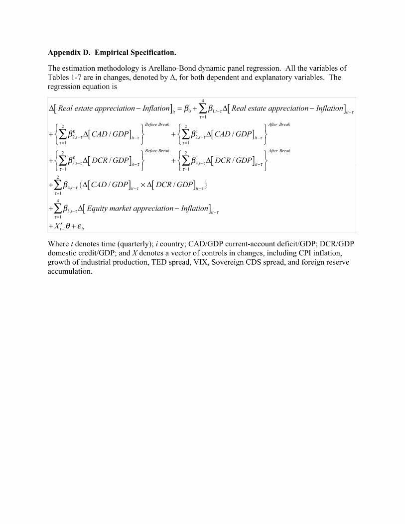
Appendix D. Empirical Specification.

The estimation methodology is Arellano-Bond dynamic panel regression. All the variables of Tables 1-7 are in changes, denoted by Δ, for both dependent and explanatory variables. The regression equation is

∆ Real estate appreciation− Inflation[ ]it= β0 + β1,t−τ∆ Real estate appreciation− Inflation[ ]

it−ττ=1

4

∑

+ β2,t−τ0 ∆ CAD / GDP[ ]

it−ττ=1

2

∑

Before Break

+ β2,t−τ1 ∆ CAD / GDP[ ]

it−ττ=1

2

∑

After Break

+ β3,t−τ0 ∆ DCR / GDP[ ]

it−ττ=1

2

∑

Before Break

+ β3,t−τ1 ∆ DCR / GDP[ ]

it−ττ=1

2

∑

After Break

+ β4,t−τ {∆ CAD / GDP[ ]it−τ

× ∆ DCR / GDP[ ]it−τ

}τ=1

2

∑

+ β5,t−τ∆ Equity market appreciation− Inflation[ ]it−τ

τ=1

4

∑+ ′X t−1θ + ε it

Where t denotes time (quarterly); i country; CAD/GDP current-account deficit/GDP; DCR/GDP domestic credit/GDP; and X denotes a vector of controls in changes, including CPI inflation, growth of industrial production, TED spread, VIX, Sovereign CDS spread, and foreign reserve accumulation.

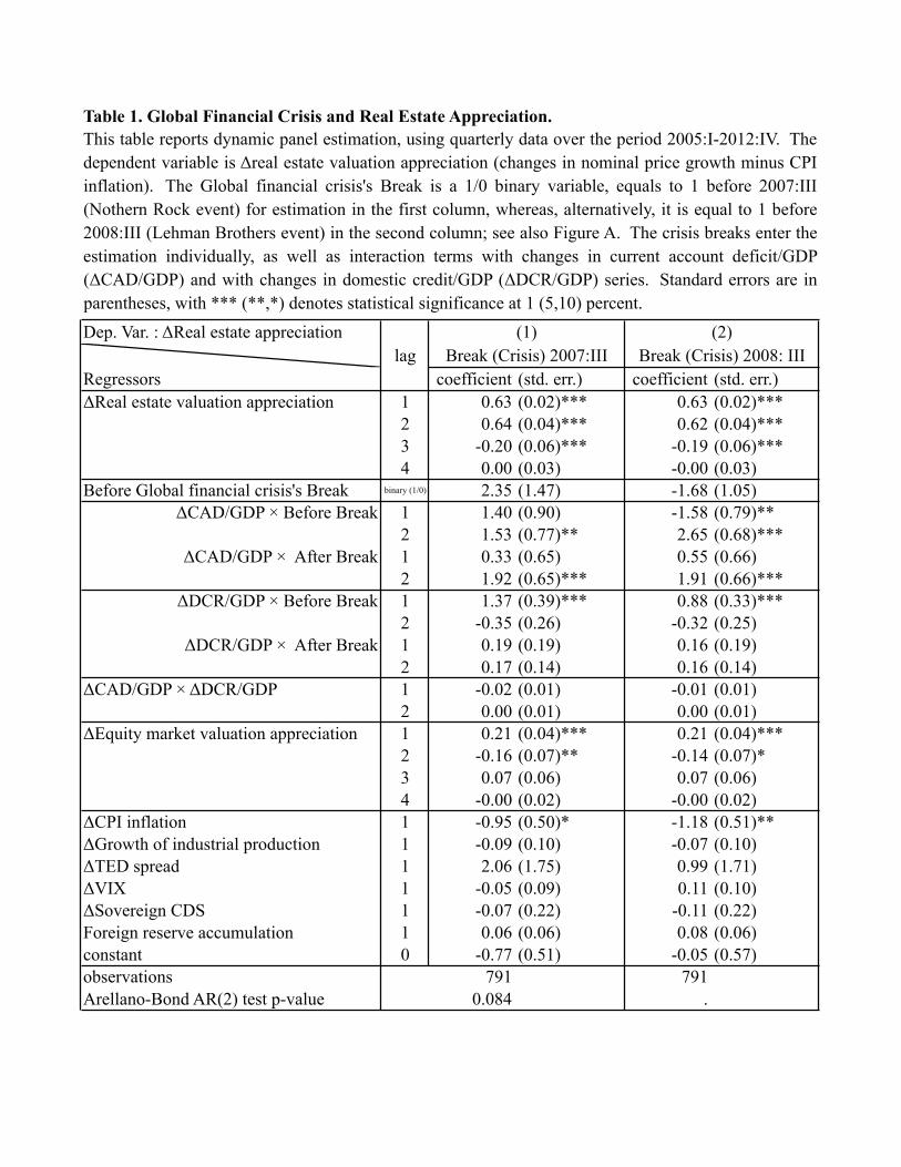
Table 1. Global Financial Crisis and Real Estate Appreciation.

Dep. Var. : ΔReal estate appreciation

Regressors coefficient (std. err.) coefficient (std. err.)

ΔReal estate valuation appreciation 1 0.63 (0.02)*** 0.63 (0.02)***

2 0.64 (0.04)*** 0.62 (0.04)***

3 -0.20 (0.06)*** -0.19 (0.06)***

4 0.00 (0.03) -0.00 (0.03)

Before Global financial crisis's Break binary (1/0) 2.35 (1.47) -1.68 (1.05)

ΔCAD/GDP × Before Break 1 1.40 (0.90) -1.58 (0.79)**

2 1.53 (0.77)** 2.65 (0.68)***

ΔCAD/GDP × After Break 1 0.33 (0.65) 0.55 (0.66)

2 1.92 (0.65)*** 1.91 (0.66)***

ΔDCR/GDP × Before Break 1 1.37 (0.39)*** 0.88 (0.33)***

2 -0.35 (0.26) -0.32 (0.25)

ΔDCR/GDP × After Break 1 0.19 (0.19) 0.16 (0.19)

2 0.17 (0.14) 0.16 (0.14)

ΔCAD/GDP × ΔDCR/GDP 1 -0.02 (0.01) -0.01 (0.01)

2 0.00 (0.01) 0.00 (0.01)

ΔEquity market valuation appreciation 1 0.21 (0.04)*** 0.21 (0.04)***

2 -0.16 (0.07)** -0.14 (0.07)*

3 0.07 (0.06) 0.07 (0.06)

4 -0.00 (0.02) -0.00 (0.02)

ΔCPI inflation 1 -0.95 (0.50)* -1.18 (0.51)**

ΔGrowth of industrial production 1 -0.09 (0.10) -0.07 (0.10)

ΔTED spread 1 2.06 (1.75) 0.99 (1.71)

ΔVIX 1 -0.05 (0.09) 0.11 (0.10)

ΔSovereign CDS 1 -0.07 (0.22) -0.11 (0.22)

Foreign reserve accumulation 1 0.06 (0.06) 0.08 (0.06)

constant 0 -0.77 (0.51) -0.05 (0.57)

observations 791 791

Arellano-Bond AR(2) test p-value 0.084 .

This table reports dynamic panel estimation, using quarterly data over the period 2005:I-2012:IV. The

dependent variable is Δreal estate valuation appreciation (changes in nominal price growth minus CPI

inflation). The Global financial crisis's Break is a 1/0 binary variable, equals to 1 before 2007:III

(Nothern Rock event) for estimation in the first column, whereas, alternatively, it is equal to 1 before

2008:III (Lehman Brothers event) in the second column; see also Figure A. The crisis breaks enter the

estimation individually, as well as interaction terms with changes in current account deficit/GDP

(ΔCAD/GDP) and with changes in domestic credit/GDP (ΔDCR/GDP) series. Standard errors are in

parentheses, with *** (**,*) denotes statistical significance at 1 (5,10) percent.

lag

(1) (2)

Break (Crisis) 2007:III Break (Crisis) 2008: III

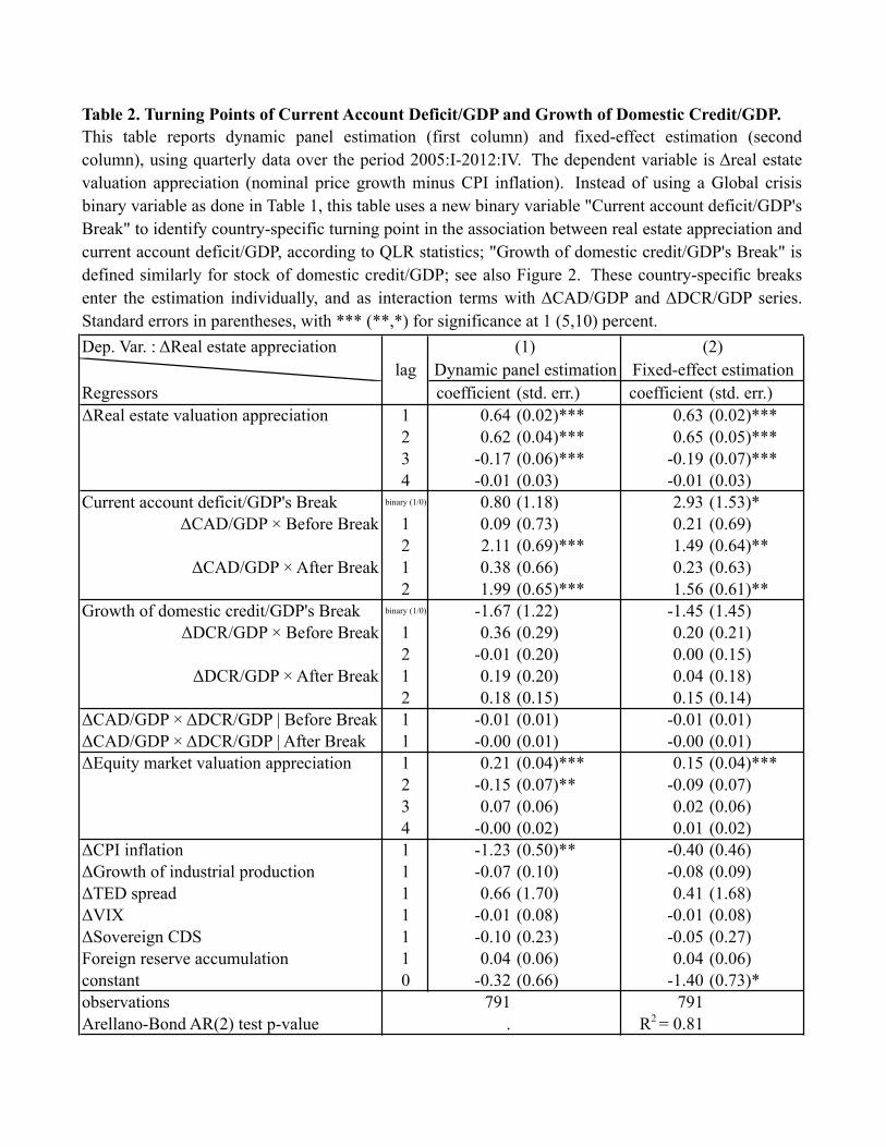
Table 2. Turning Points of Current Account Deficit/GDP and Growth of Domestic Credit/GDP.




2 0.62 (0.04)*** 0.65 (0.05)***

3 -0.17 (0.06)*** -0.19 (0.07)***

4 -0.01 (0.03) -0.01 (0.03)

Current account deficit/GDP's Break binary (1/0) 0.80 (1.18) 2.93 (1.53)*

ΔCAD/GDP × Before Break 1 0.09 (0.73) 0.21 (0.69)

2 2.11 (0.69)*** 1.49 (0.64)**

ΔCAD/GDP × After Break 1 0.38 (0.66) 0.23 (0.63)

2 1.99 (0.65)*** 1.56 (0.61)**

Growth of domestic credit/GDP's Break binary (1/0) -1.67 (1.22) -1.45 (1.45)

ΔDCR/GDP × Before Break 1 0.36 (0.29) 0.20 (0.21)

2 -0.01 (0.20) 0.00 (0.15)

ΔDCR/GDP × After Break 1 0.19 (0.20) 0.04 (0.18)

2 0.18 (0.15) 0.15 (0.14)

ΔCAD/GDP × ΔDCR/GDP | Before Break 1 -0.01 (0.01) -0.01 (0.01)

ΔCAD/GDP × ΔDCR/GDP | After Break 1 -0.00 (0.01) -0.00 (0.01)


2 -0.15 (0.07)** -0.09 (0.07)

3 0.07 (0.06) 0.02 (0.06)

4 -0.00 (0.02) 0.01 (0.02)

ΔCPI inflation 1 -1.23 (0.50)** -0.40 (0.46)


ΔTED spread 1 0.66 (1.70) 0.41 (1.68)

ΔVIX 1 -0.01 (0.08) -0.01 (0.08)

ΔSovereign CDS 1 -0.10 (0.23) -0.05 (0.27)


constant 0 -0.32 (0.66) -1.40 (0.73)*


Arellano-Bond AR(2) test p-value . R2 = 0.81

This table reports dynamic panel estimation (first column) and fixed-effect estimation (second

column), using quarterly data over the period 2005:I-2012:IV. The dependent variable is Δreal estate

valuation appreciation (nominal price growth minus CPI inflation). Instead of using a Global crisis

binary variable as done in Table 1, this table uses a new binary variable "Current account deficit/GDP's

Break" to identify country-specific turning point in the association between real estate appreciation and

current account deficit/GDP, according to QLR statistics; "Growth of domestic credit/GDP's Break" is

defined similarly for stock of domestic credit/GDP; see also Figure 2. These country-specific breaks

enter the estimation individually, and as interaction terms with ΔCAD/GDP and ΔDCR/GDP series.

Standard errors in parentheses, with *** (**,*) for significance at 1 (5,10) percent.

lag

(1)

Dynamic panel estimation

(2)

Fixed-effect estimation

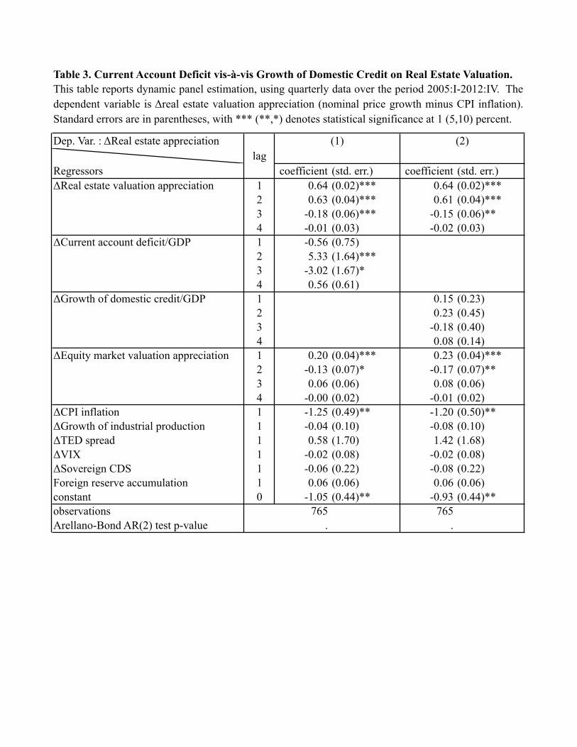
Table 3. Current Account Deficit vis-à-vis Growth of Domestic Credit on Real Estate Valuation.




2 0.63 (0.04)*** 0.61 (0.04)***

3 -0.18 (0.06)*** -0.15 (0.06)**

4 -0.01 (0.03) -0.02 (0.03)

ΔCurrent account deficit/GDP 1 -0.56 (0.75)

2 5.33 (1.64)***

3 -3.02 (1.67)*

4 0.56 (0.61)

ΔGrowth of domestic credit/GDP 1 0.15 (0.23)

2 0.23 (0.45)

3 -0.18 (0.40)

4 0.08 (0.14)


2 -0.13 (0.07)* -0.17 (0.07)**

3 0.06 (0.06) 0.08 (0.06)

4 -0.00 (0.02) -0.01 (0.02)

ΔCPI inflation 1 -1.25 (0.49)** -1.20 (0.50)**


ΔTED spread 1 0.58 (1.70) 1.42 (1.68)

ΔVIX 1 -0.02 (0.08) -0.02 (0.08)

ΔSovereign CDS 1 -0.06 (0.22) -0.08 (0.22)


constant 0 -1.05 (0.44)** -0.93 (0.44)**


Arellano-Bond AR(2) test p-value . .


dependent variable is Δreal estate valuation appreciation (nominal price growth minus CPI inflation).

Standard errors are in parentheses, with *** (**,*) denotes statistical significance at 1 (5,10) percent.

lag

(1) (2)

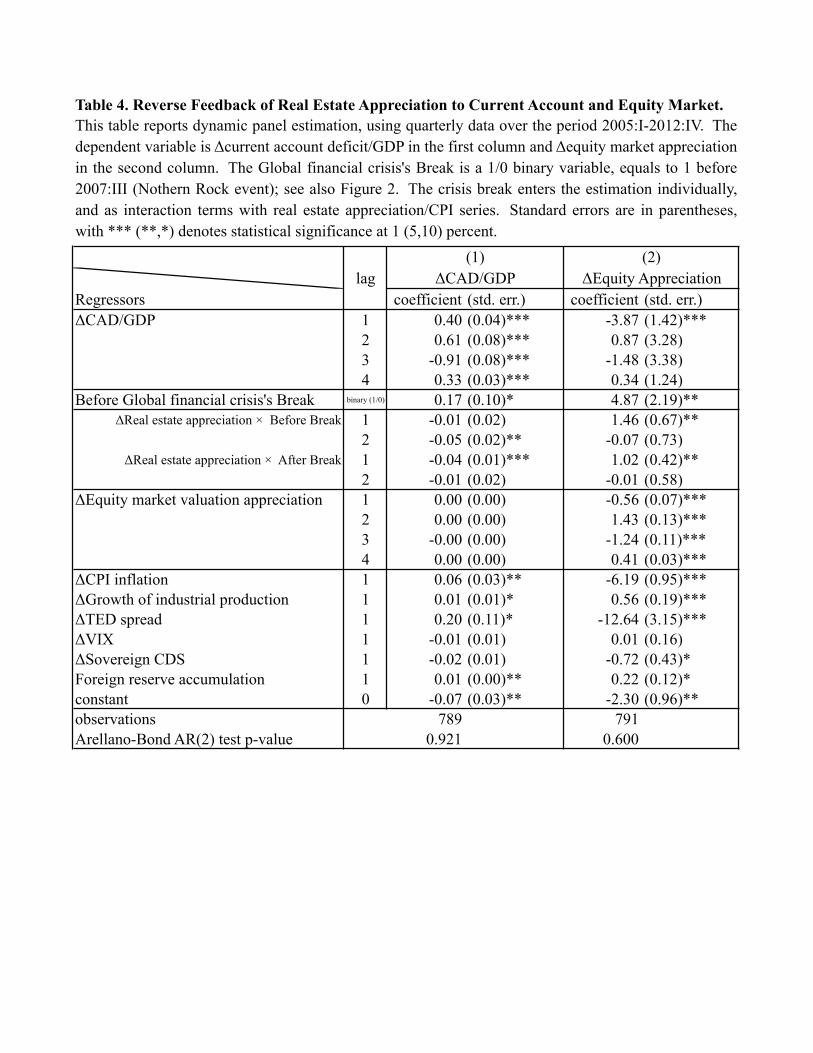
Table 4. Reverse Feedback of Real Estate Appreciation to Current Account and Equity Market.


ΔCAD/GDP 1 0.40 (0.04)*** -3.87 (1.42)***

2 0.61 (0.08)*** 0.87 (3.28)

3 -0.91 (0.08)*** -1.48 (3.38)

4 0.33 (0.03)*** 0.34 (1.24)

Before Global financial crisis's Break binary (1/0) 0.17 (0.10)* 4.87 (2.19)**

ΔReal estate appreciation × Before Break 1 -0.01 (0.02) 1.46 (0.67)**

2 -0.05 (0.02)** -0.07 (0.73)

ΔReal estate appreciation × After Break 1 -0.04 (0.01)*** 1.02 (0.42)**

2 -0.01 (0.02) -0.01 (0.58)

ΔEquity market valuation appreciation 1 0.00 (0.00) -0.56 (0.07)***

2 0.00 (0.00) 1.43 (0.13)***

3 -0.00 (0.00) -1.24 (0.11)***

4 0.00 (0.00) 0.41 (0.03)***

ΔCPI inflation 1 0.06 (0.03)** -6.19 (0.95)***

ΔGrowth of industrial production 1 0.01 (0.01)* 0.56 (0.19)***

ΔTED spread 1 0.20 (0.11)* -12.64 (3.15)***

ΔVIX 1 -0.01 (0.01) 0.01 (0.16)

ΔSovereign CDS 1 -0.02 (0.01) -0.72 (0.43)*

Foreign reserve accumulation 1 0.01 (0.00)** 0.22 (0.12)*

constant 0 -0.07 (0.03)** -2.30 (0.96)**


Arellano-Bond AR(2) test p-value 0.921 0.600


dependent variable is Δcurrent account deficit/GDP in the first column and Δequity market appreciation

in the second column. The Global financial crisis's Break is a 1/0 binary variable, equals to 1 before

2007:III (Nothern Rock event); see also Figure 2. The crisis break enters the estimation individually,

and as interaction terms with real estate appreciation/CPI series. Standard errors are in parentheses,

with *** (**,*) denotes statistical significance at 1 (5,10) percent.

lag

(1) (2)

ΔCAD/GDP ΔEquity Appreciation

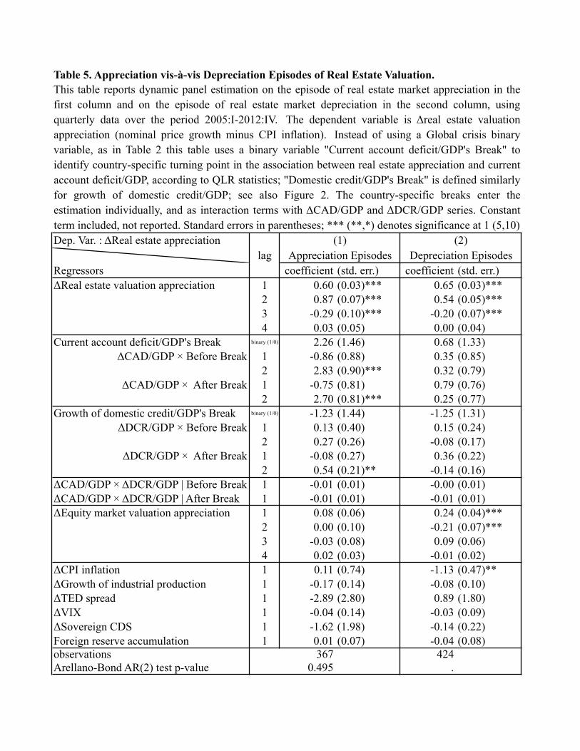
Table 5. Appreciation vis-à-vis Depreciation Episodes of Real Estate Valuation.




2 0.87 (0.07)*** 0.54 (0.05)***

3 -0.29 (0.10)*** -0.20 (0.07)***

4 0.03 (0.05) 0.00 (0.04)

Current account deficit/GDP's Break binary (1/0) 2.26 (1.46) 0.68 (1.33)

ΔCAD/GDP × Before Break 1 -0.86 (0.88) 0.35 (0.85)

2 2.83 (0.90)*** 0.32 (0.79)

ΔCAD/GDP × After Break 1 -0.75 (0.81) 0.79 (0.76)

2 2.70 (0.81)*** 0.25 (0.77)

Growth of domestic credit/GDP's Break binary (1/0) -1.23 (1.44) -1.25 (1.31)

ΔDCR/GDP × Before Break 1 0.13 (0.40) 0.15 (0.24)

2 0.27 (0.26) -0.08 (0.17)

ΔDCR/GDP × After Break 1 -0.08 (0.27) 0.36 (0.22)

2 0.54 (0.21)** -0.14 (0.16)



ΔEquity market valuation appreciation 1 0.08 (0.06) 0.24 (0.04)***

2 0.00 (0.10) -0.21 (0.07)***

3 -0.03 (0.08) 0.09 (0.06)

4 0.02 (0.03) -0.01 (0.02)

ΔCPI inflation 1 0.11 (0.74) -1.13 (0.47)**


ΔTED spread 1 -2.89 (2.80) 0.89 (1.80)

ΔVIX 1 -0.04 (0.14) -0.03 (0.09)

ΔSovereign CDS 1 -1.62 (1.98) -0.14 (0.22)

Foreign reserve accumulation 1 0.01 (0.07) -0.04 (0.08)


Arellano-Bond AR(2) test p-value 0.495 .

This table reports dynamic panel estimation on the episode of real estate market appreciation in the

first column and on the episode of real estate market depreciation in the second column, using

quarterly data over the period 2005:I-2012:IV. The dependent variable is Δreal estate valuation

appreciation (nominal price growth minus CPI inflation). Instead of using a Global crisis binary

variable, as in Table 2 this table uses a binary variable "Current account deficit/GDP's Break" to

identify country-specific turning point in the association between real estate appreciation and current

account deficit/GDP, according to QLR statistics; "Domestic credit/GDP's Break" is defined similarly

for growth of domestic credit/GDP; see also Figure 2. The country-specific breaks enter the

estimation individually, and as interaction terms with ΔCAD/GDP and ΔDCR/GDP series. Constant

term included, not reported. Standard errors in parentheses; *** (**,*) denotes significance at 1 (5,10)

lag

(1) (2)

Appreciation Episodes Depreciation Episodes

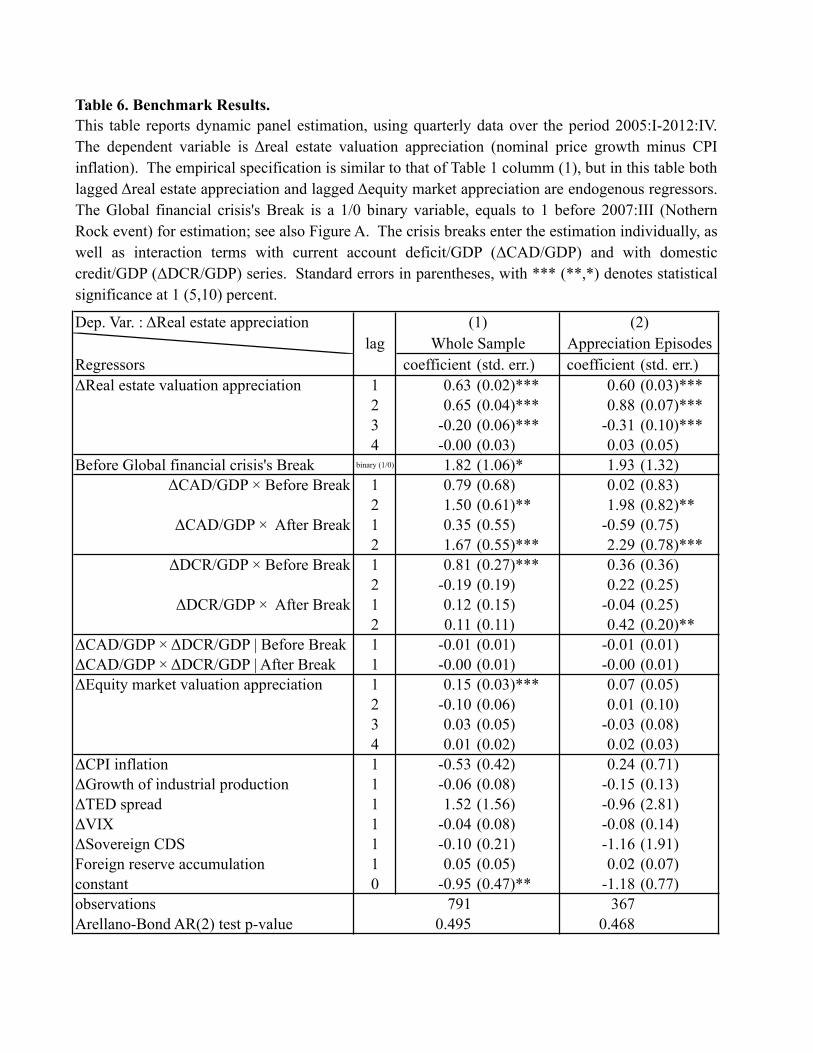
Table 6. Benchmark Results.




2 0.65 (0.04)*** 0.88 (0.07)***

3 -0.20 (0.06)*** -0.31 (0.10)***

4 -0.00 (0.03) 0.03 (0.05)

Before Global financial crisis's Break binary (1/0) 1.82 (1.06)* 1.93 (1.32)

ΔCAD/GDP × Before Break 1 0.79 (0.68) 0.02 (0.83)

2 1.50 (0.61)** 1.98 (0.82)**

ΔCAD/GDP × After Break 1 0.35 (0.55) -0.59 (0.75)

2 1.67 (0.55)*** 2.29 (0.78)***

ΔDCR/GDP × Before Break 1 0.81 (0.27)*** 0.36 (0.36)

2 -0.19 (0.19) 0.22 (0.25)

ΔDCR/GDP × After Break 1 0.12 (0.15) -0.04 (0.25)

2 0.11 (0.11) 0.42 (0.20)**



ΔEquity market valuation appreciation 1 0.15 (0.03)*** 0.07 (0.05)

2 -0.10 (0.06) 0.01 (0.10)

3 0.03 (0.05) -0.03 (0.08)

4 0.01 (0.02) 0.02 (0.03)

ΔCPI inflation 1 -0.53 (0.42) 0.24 (0.71)


ΔTED spread 1 1.52 (1.56) -0.96 (2.81)

ΔVIX 1 -0.04 (0.08) -0.08 (0.14)

ΔSovereign CDS 1 -0.10 (0.21) -1.16 (1.91)


constant 0 -0.95 (0.47)** -1.18 (0.77)


Arellano-Bond AR(2) test p-value 0.495 0.468

This table reports dynamic panel estimation, using quarterly data over the period 2005:I-2012:IV.

The dependent variable is Δreal estate valuation appreciation (nominal price growth minus CPI

inflation). The empirical specification is similar to that of Table 1 columm (1), but in this table both

lagged Δreal estate appreciation and lagged Δequity market appreciation are endogenous regressors.

The Global financial crisis's Break is a 1/0 binary variable, equals to 1 before 2007:III (Nothern

Rock event) for estimation; see also Figure A. The crisis breaks enter the estimation individually, as

well as interaction terms with current account deficit/GDP (ΔCAD/GDP) and with domestic

credit/GDP (ΔDCR/GDP) series. Standard errors in parentheses, with *** (**,*) denotes statistical

significance at 1 (5,10) percent.

lag

(1) (2)

Whole Sample Appreciation Episodes

Table 7. Additional Results.


Regressors coefficient (std. err.) coefficient (std. err.) coefficient (std. err.) coefficient (std. err.) coefficient (std. err.) coefficient (std. err.) coefficient (std. err.)

ΔReal estate valuation appreciation 1 0.70 (0.02)*** 0.70 (0.02)*** 0.71 (0.02)*** 0.71 (0.02)*** 0.71 (0.02)*** 0.62 (0.02)*** 0.64 (0.03)***

2 0.57 (0.04)*** 0.57 (0.04)*** 0.60 (0.04)*** 0.79 (0.05)*** 0.80 (0.05)*** 0.89 (0.05)*** 0.58 (0.06)***

3 -0.08 (0.06) -0.08 (0.06) -0.13 (0.06)** -0.11 (0.08) -0.11 (0.08) -0.39 (0.08)*** -0.16 (0.08)*

4 -0.04 (0.03) -0.04 (0.03) -0.01 (0.03) 0.02 (0.04) 0.03 (0.04) 0.10 (0.04)** -0.01 (0.04)

Before Global financial crisis's Break binary (1/0) 2.32 (1.22)* 2.30 (1.22)* 1.92 (0.93)** 2.88 (1.04)*** 2.83 (1.03)*** -0.59 (0.88) 4.08 (1.85)**

ΔCAD/GDP × Before Break 1 1.82 (3.35) 1.05 (1.73) 5.01 (26.34) 5.83 (19.99) 9.38 (19.68) -0.33 (0.68) 1.66 (0.95)*

2 -0.48 (1.88) -0.31 (0.98) -9.21 (14.84) -10.22 (11.44) -19.43 (11.57)* 0.91 (0.63) 1.21 (0.88)

ΔCAD/GDP × After Break 1 0.39 (0.94) 0.24 (0.49) -1.62 (6.29) -0.50 (5.12) 6.32 (5.24) -0.24 (0.58) 0.97 (0.83)

2 -0.14 (0.53) -0.08 (0.28) -0.26 (3.59) -1.50 (2.96) -4.74 (3.02) 0.63 (0.59) 1.65 (0.81)**

ΔDCR/GDP × Before Break 1 0.89 (0.28)*** 0.89 (0.28)*** 0.77 (0.23)*** 0.68 (0.23)*** 0.71 (0.23)*** 0.46 (0.19)** 1.11 (0.54)**

2 -0.26 (0.19) -0.26 (0.19) -0.34 (0.16)** -0.29 (0.15)* -0.26 (0.15)* -0.27 (0.13)** -0.01 (0.36)

ΔDCR/GDP × After Break 1 0.01 (0.15) 0.01 (0.15) 0.03 (0.14) 0.00 (0.14) 0.02 (0.14) 0.10 (0.11) -0.03 (0.30)

2 0.08 (0.12) 0.07 (0.12) 0.06 (0.11) 0.02 (0.10) 0.02 (0.10) -0.04 (0.08) 0.47 (0.24)*

ΔEquity market valuation appreciation 1 0.08 (0.04)* 0.08 (0.04)* 0.10 (0.03)*** 0.05 (0.04) 0.05 (0.04) 0.14 (0.04)*** 0.15 (0.05)***

2 -0.00 (0.07) -0.00 (0.07) -0.02 (0.06) -0.00 (0.07) 0.01 (0.07) -0.18 (0.06)*** -0.02 (0.10)

3 -0.01 (0.06) -0.02 (0.06) -0.01 (0.05) 0.02 (0.06) 0.02 (0.06) 0.14 (0.05)*** -0.06 (0.08)

4 0.01 (0.02) 0.01 (0.02) 0.02 (0.01) -0.00 (0.02) -0.00 (0.02) -0.03 (0.02)* 0.04 (0.03)

ΔCPI inflation 1 -0.32 (0.53) -0.30 (0.53) 0.37 (0.43) 1.48 (0.59)** 1.45 (0.58)** -0.14 (0.51) -0.12 (0.60)

ΔGrowth of industrial production 1 0.38 (0.13)*** 0.38 (0.13)*** 0.16 (0.10) 0.15 (0.12) 0.14 (0.11) -0.03 (0.10) -0.15 (0.12)

ΔTED spread 1 3.20 (1.67)* 3.18 (1.67)* 2.95 (1.44)** 1.75 (1.66) 1.62 (1.63) 1.49 (1.35) -0.98 (2.88)

ΔVIX 1 -0.03 (0.08) -0.03 (0.08) -0.04 (0.07) -0.06 (0.08) -0.06 (0.08) -0.06 (0.07) 0.03 (0.14)

ΔSovereign CDS 1 -0.11 (0.18) -0.11 (0.18) -0.12 (0.17) -0.06 (0.15) -0.06 (0.15) -0.08 (0.13) -1.57 (1.45)

Foreign reserve accumulation 1 0.02 (0.06) 0.02 (0.06) 0.02 (0.05) 0.07 (0.06) 0.07 (0.06) 0.03 (0.05) 0.04 (0.09)

constant 0 -0.67 (0.49) -0.67 (0.49) -0.93 (0.42)** -1.27 (0.47)*** -1.26 (0.46)*** -1.01 (0.40)** -1.03 (0.83)

observations 523 523 588 383 383 398 393

Arellano-Bond AR(2) test p-value 0.348 0.337 . 0.688 0.633 0.445 0.529


Regressors coefficient (std. err.) coefficient (std. err.) coefficient (std. err.) coefficient (std. err.) coefficient (std. err.) coefficient (std. err.) coefficient (std. err.)

ΔReal estate valuation appreciation 1 0.60 (0.02)*** 0.72 (0.04)*** 0.66 (0.02)*** 0.63 (0.03)*** 0.66 (0.02)*** 0.61 (0.04)*** 0.64 (0.02)***

2 0.64 (0.05)*** 0.64 (0.08)*** 0.80 (0.06)*** 0.61 (0.05)*** 0.76 (0.05)*** 0.51 (0.07)*** 0.64 (0.04)***

3 -0.23 (0.07)*** -0.06 (0.13) -0.34 (0.09)*** -0.18 (0.07)** -0.18 (0.08)** -0.15 (0.10) -0.19 (0.06)***

4 0.01 (0.03) -0.06 (0.07) 0.10 (0.05)** -0.01 (0.04) -0.04 (0.04) 0.00 (0.05) -0.00 (0.03)

Before Global financial crisis's Break binary (1/0) 0.77 (1.17) 3.64 (2.18)* 0.34 (0.95) 2.52 (1.51)* 2.53 (1.07)** -2.08 (2.49) 1.71 (1.05)

ΔCAD/GDP × Before Break 1 0.79 (0.75) 0.61 (1.05) -1.21 (0.82) 1.49 (0.79)* -0.00 (0.81) 1.55 (1.03) 0.83 (0.67)

2 0.91 (0.69) 3.22 (1.11)*** -0.22 (0.78) 1.26 (0.74)* 0.62 (0.74) 1.79 (0.99)* 1.52 (0.61)**

ΔCAD/GDP × After Break 1 0.63 (0.65) 0.28 (0.93) -1.17 (0.73) 0.87 (0.68) 0.00 (0.72) 1.15 (0.90) 0.33 (0.54)

2 1.03 (0.63) 3.41 (1.03)*** -0.65 (0.75) 1.69 (0.67)** 0.42 (0.69) 2.27 (0.91)** 1.72 (0.55)***

ΔDCR/GDP × Before Break 1 0.61 (0.27)** 1.00 (0.74) 0.25 (0.20) 1.10 (0.43)*** 0.82 (0.26)*** -0.18 (0.71) 0.76 (0.27)***

2 -0.15 (0.18) -0.27 (0.51) -0.28 (0.13)** -0.12 (0.29) -0.28 (0.18) 0.45 (0.45) -0.15 (0.18)

ΔDCR/GDP × After Break 1 0.09 (0.15) -0.18 (0.48) 0.03 (0.11) 0.05 (0.24) 0.05 (0.15) 0.13 (0.33) 0.12 (0.15)

2 0.14 (0.11) -0.19 (0.40) -0.04 (0.08) 0.32 (0.19)* 0.10 (0.11) 0.06 (0.27) 0.11 (0.11)

ΔEquity market valuation appreciation 1 0.19 (0.04)*** 0.11 (0.06)* 0.13 (0.04)*** 0.17 (0.04)*** 0.06 (0.04) 0.24 (0.06)*** 0.16 (0.03)***

2 -0.13 (0.07)* -0.02 (0.11) -0.14 (0.07)* -0.08 (0.08) -0.03 (0.07) -0.12 (0.12) -0.10 (0.06)

3 0.06 (0.06) -0.02 (0.10) 0.10 (0.06)* 0.00 (0.07) 0.04 (0.06) -0.02 (0.10) 0.03 (0.05)

4 -0.00 (0.02) 0.01 (0.03) -0.01 (0.02) 0.01 (0.02) -0.01 (0.02) 0.04 (0.03) 0.01 (0.02)

ΔCPI inflation 1 -0.05 (0.50) 0.59 (0.75) 1.35 (0.65)** -0.62 (0.50) 0.36 (0.59) -0.90 (0.65) -0.45 (0.41)

ΔGrowth of industrial production 1 0.12 (0.10) -0.57 (0.17)*** 0.03 (0.11) -0.13 (0.11) 0.27 (0.11)** -0.34 (0.14)** -0.06 (0.09)

ΔTED spread 1 1.84 (1.71) -5.14 (3.69) 1.03 (1.50) -0.05 (2.31) 1.40 (1.60) -2.01 (3.72)

ΔVIX 1 -0.04 (0.09) 0.17 (0.18) -0.02 (0.08) -0.01 (0.11) 0.03 (0.08) -0.04 (0.17) 0.01 (0.05)

ΔSovereign CDS 1 -0.06 (0.20) -2.44 (1.82) -0.10 (0.12) -0.84 (1.16) -0.07 (0.18) -1.52 (1.60) -0.12 (0.21)

Foreign reserve accumulation 1 0.14 (0.06)** -0.09 (0.10) -0.13 (0.37) 0.04 (0.06) 0.06 (0.06) 0.03 (0.09) 0.05 (0.05)

Growth of Mortgage Origination in USA 1 0.00 (0.00)

constant 0 -1.03 (0.51)** -0.80 (1.01) -1.19 (0.51)** -0.86 (0.64) -1.25 (0.48)*** -0.19 (1.08) -0.99 (0.47)**

observations 613 178 268 523 572 219 791

Arellano-Bond AR(2) test p-value 0.589 0.056 0.674 0.459 0.961 0.465 0.348

lag

(13) (14)

High Financial Openness Low Financial Openness Euro Area Countries Non Euro Countries OECD Countries Non OECD Episodes Whole Sample

(8) (9) (10) (11) (12)

(7)

No Banking Crisis Group

(4)

CAD=Debt Inflows CAD=Net Debt Flows

(5) (6)

This table reports dynamic panel estimation, using quarterly data over the period 2005:I-2012:IV. The dependent variable is Δreal estate valuation appreciation (nominal price growth minus CPI inflation). The empirical specification is

similar to that of Table 1 columm (1), but in this table both lagged Δreal estate appreciation and lagged Δequity market appreciation are endogenous regressors. The Global financial crisis's Break is a 1/0 binary variable, equals to 1 before

2007:III (Nothern Rock event) for estimation; see also Figure A. The crisis breaks enter the estimation individually, as well as interaction terms with current account deficit/GDP (ΔCAD/GDP) and with domestic credit/GDP (ΔDCR/GDP)

series. Standard errors in parentheses, with *** (**,*) denotes statistical significance at 1 (5,10) percent.

CAD=Debt In+Outflows Banking Crisis Grouplag

(1) (2)

CAD=Gross Inflows CAD=Inflows+Outflows

(3)

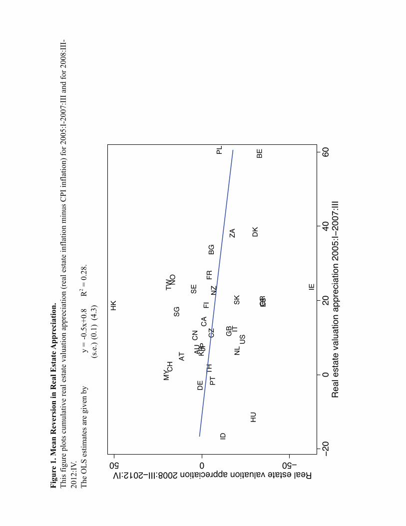
Fig

ure

1. M

ean

Rev

ersi

on

in

Rea

l E

state

Ap

pre

ciati

on

.

The

OL

S e

stim

ates

are

giv

en b

yy =

-0.5

x+

0.8

R2 =

0.2

8.

(s.e

.)(0

.1)

(4.3

)

This

fig

ure

plo

ts c

um

ula

tive

real

est

ate

val

uat

ion a

ppre

ciat

ion (

real

est

ate

infl

atio

n m

inus

CP

I in

flat

ion)

for

2005:I

-2007:I

II a

nd f

or

2008:I

II-

2012:I

V.

!" !#

$%

$&

'!

'(

') '*

+%

+,

%-

./

.0

&$

&0

(,

(#

/+

/%

/"

12

,0

34

)5

)6

)*

25

2"

-%

-&

-,

"(

"7

#-

*!

899890:;<=:>?;?:=@;<A;?BCD=;EEF:GB;?BCD=H99IJ///H9KHJ/L

H9

9H9

M9

N9

0:;<=:>?;?:=@;<A;?BCD=;EEF:GB;?BCD=H998J/H99OJ///

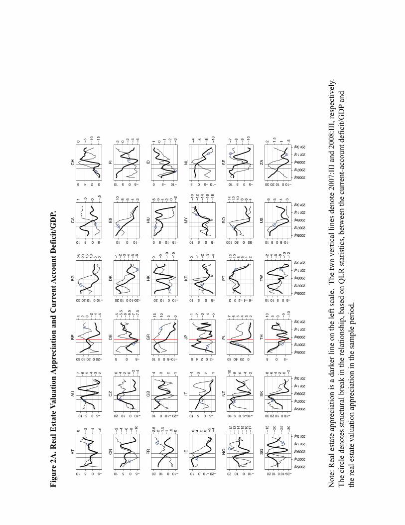
Fig

ure

2A

. R

eal

Est

ate

Valu

ati

on

Ap

pre

ciati

on

an

d C

urr

ent

Acc

ou

nt

Def

icit

/GD

P.

Note

: R

eal

esta

te a

ppre

ciat

ion i

s a

dar

ker

lin

e on t

he

left

sca

le. T

he

two v

erti

cal

lines

den

ote

2007:I

II a

nd 2

008:I

II, re

spec

tivel

y.

The

circ

le d

enote

s st

ruct

ura

l bre

ak i

n t

he

rela

tionsh

ip, bas

ed o

n Q

LR

sta

tist

ics,

bet

wee

n t

he

curr

ent-

acco

unt

def

icit

/GD

P a

nd

the

real

est

ate

val

uat

ion a

ppre

ciat

ion i

n t

he

sam

ple

per

iod.

!"#

$

#%"&!'

!"#$#"

$&($(&#$#&

)&

$)&(

(&

($

&

$

($

*!"#

"#

$#"!

')&'!)&!&)&&

!&"%#(

#"!*($

!"#

$#

$)&(()&

##)&

(#%"

$&($

(&

(&

($

&

$

#

$#"!*

%#(

$(

"#$#"!

(#%"

&"%#(

"%#(

$

(*

(!

("

(#

($

($

*!"

('(!(&("(%(#

#"!*($

#%"&!'

#"!*($(#

"!*($(#("

($

+*'

%$

#&

#$

(&

#$#"!*

($

&

$&($

(#

($

*!"#

%"&!

)&(()&

#

&$&($

&$&($

#$$#$"$!$

($$($#$%$

&$&($

$#"!

&$&($

($$($#$

&$&

#$($$($#$

($$($

&$&($

($$($#$

#$($$($

($&$&($

($$($#$

(&($&$

($&$

#$($$($

&$&($

#$#"!

&$&($

&$&($

($&$&

($$($#$

($&$&($

$#$"$!$

!"#$#

&$$&$($$

&$&($

#$($$($#$

($$($#$%$

&$&

&$&($(&

($&$&($

($$($#$%$

#$$&,(

#$$',(

#$$+,(

#$((,(

#$(%,(

#$$&,(

#$$',(

#$$+,(

#$((,(

#$(%,(

#$$&,(

#$$',(

#$$+,(

#$((,(

#$(%,(

#$$&,(

#$$',(

#$$+,(

#$((,(

#$(%,(

#$$&,(

#$$',(

#$$+,(

#$((,(

#$(%,(

#$$&,(

#$$',(

#$$+,(

#$((,(

#$(%,(

-.

-/

01

02

3-

34

35

36

71

78

19

:;

:<

20

2<

48

4/

;7

;1;.

=>

8<

?@

5A

5B

56

>A

>.

<B

91

92

98

.4

.C

/9

6-

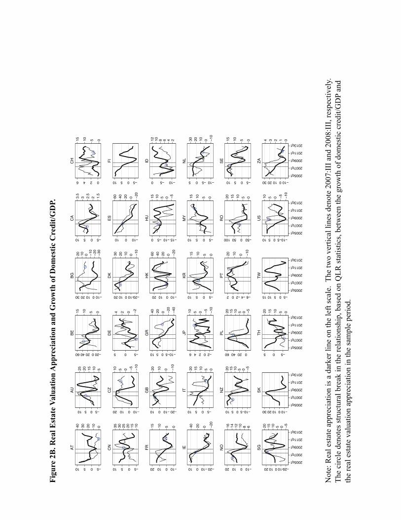
Fig

ure

2B

. R

eal

Est

ate

Valu

ati

on

Ap

pre

ciati

on

an

d G

row

th o

f D

om

esti

c C

red

it/G

DP

.

Note

: R

eal

esta

te a

ppre

ciat

ion i

s a

dar

ker

lin

e on t

he

left

sca

le. T

he

two v

erti

cal

lines

den

ote

2007:I

II a

nd 2

008:I

II, re

spec

tivel

y.

The

circ

le d

enote

s st

ruct

ura

l bre

ak i

n t

he

rela

tionsh

ip, bas

ed o

n Q

LR

sta

tist

ics,

bet

wee

n t

he

gro

wth

of

dom

esti

c cr

edit

/GD

P a

nd

the

real

est

ate

val

uat

ion a

ppre

ciat

ion i

n t

he

sam

ple

per

iod.

!"!

#!

$!

%!

&"!

"&

#!

#&

!&"!

"&

$!#!"!

!"!#!

"'&

##'&

$$'&

!&"!

"&

"!"&#!#&$!$&

"!

&

!&"!

#

!#%

"!

!"!

#!

$!

#!

!#!

%!

(!

!&"!

"&

"!

!"!

#!

%!

#!

!#!

%!

#!

!#!

%!

(!

&

!&"!

"&

#%()"!"#

#!

!#!

%!

!&"!

"&

#!

"!

&

!&"!

!&"!

"&

!&"!

"&

"!

!"!

#!

$!

()"!"#"%"(

&!&"!"&#!

&!&"!"&#!

"!

!"!

#!

!&"!

"&

#!

!&"!

"&

&

!&"!

"&

#!

!&"!

"&

#!

"!

&

!&"!

!"#$%

&!&"!

&!&"!

#!!#!%!(!

"!!"!#!$!

&!&"!

!#%(

&!&"!

"!!"!#!

&!&

#!"!!"!#!

"!!"!

&!&"!

"!!"!#!

#!"!!"!

"!&!&"!

"!!"!#!

"&"!&!

"!&!

#!"!!"!

&!&"!

#!#%(

&!&"!

&!&"!

"!&!&

"!!"!#!

"!&!&"!

!#!%!(!

(%#!#

&!!&!"!!

&!&"!

#!"!!"!#!

"!!"!#!$!

&!&

&!&"!"&

"!&!&"!

"!!"!#!$!

#!!&*"

#!!+*"

#!!,*"

#!""*"

#!"$*"

#!!&*"

#!!+*"

#!!,*"

#!""*"

#!"$*"

#!!&*"

#!!+*"

#!!,*"

#!""*"

#!"$*"

#!!&*"

#!!+*"

#!!,*"

#!""*"

#!"$*"

#!!&*"

#!!+*"

#!!,*"

#!""*"

#!"$*"

#!!&*"

#!!+*"

#!!,*"

#!""*"

#!"$*"

-.

-/

01

02

3-

34

35

36

71

78

19

:;

:<

20

2<

48

4/

;7

;1;.

=>

8<

?@

5A

5B

56

>A

>.

<B

91

92

98

.4

.C

/9

6-

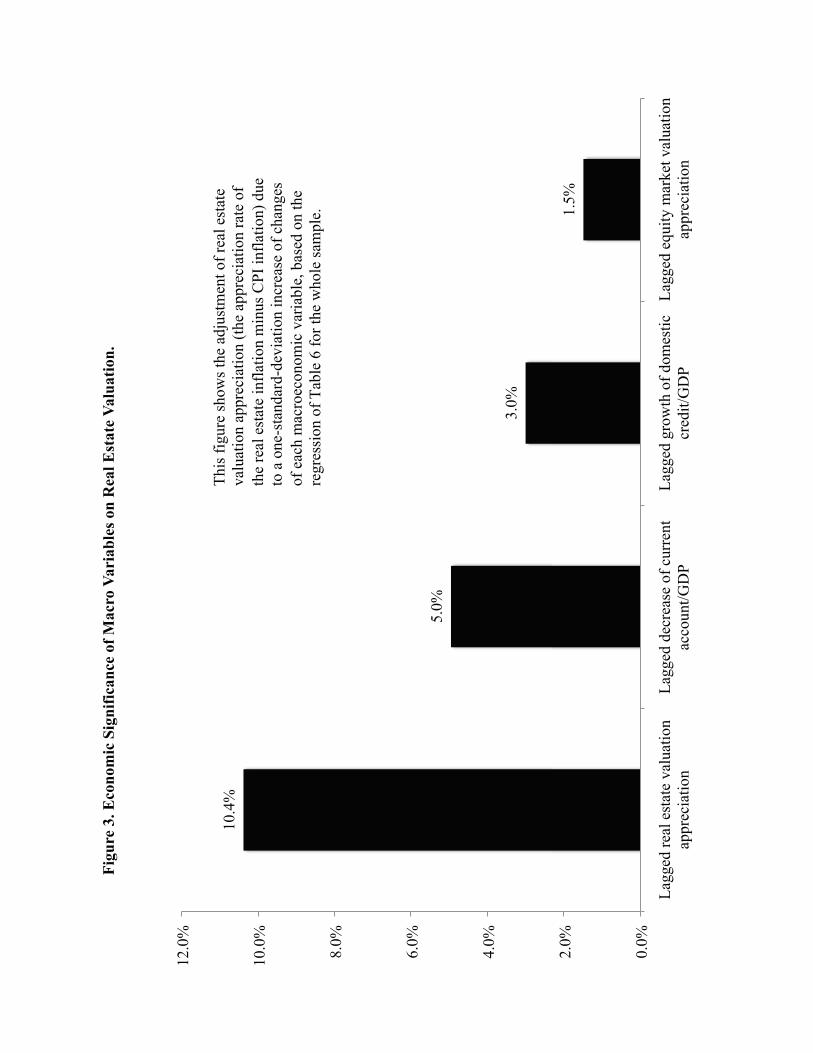
10.4

%

5.0

%

3.0

%

1.5

%

0.0

%

2.0

%

4.0

%

6.0

%

8.0

%

10.0

%

12.0

%

Lag

ged

rea

l es

tate

val

uat

ion

appre

ciat

ion

Lag

ged

dec

reas

e of

curr

ent

acco

unt/

GD

P

Lag

ged

gro

wth

of

dom

esti

c

cred

it/G

DP

Lag

ged

equit

y m

arket

val

uat

ion

appre

ciat

ion

Fig

ure

3. E

con

om

ic S

ign

ific

an

ce o

f M

acr

o V

ari

ab

les

on

Rea

l E

state

Valu

ati

on

.

This

fig

ure

show

s th

e ad

just

men

t of

real

est

ate

val

uat

ion a

ppre

ciat

ion (

the

appre

ciat

ion r

ate

of

the

real

est

ate

infl

atio

n m

inus

CP

I in

flat

ion)

due

to a

one-

stan

dar

d-d

evia

tion i

ncr

ease

of

chan

ges

of

each

mac

roec

onom

ic v

aria

ble

, bas

ed o

n t

he

regre

ssio

n o

f T

able

6 f

or

the

whole

sam

ple

.

Real Estate Valuation, Current Account and Credit …Real Estate Valuation, Current Account and...

Documents

Transcript of Real Estate Valuation, Current Account and Credit …Real Estate Valuation, Current Account and...