Reading Note on Quantum Field Theory in Curved Spacetime · Reading Note on Quantum Field Theory in...

Reading Note on Quantum Field Theory in Curved Spacetime

Zhong-Zhi Xianyu∗

Institute of Modern Physics and Center for High Energy Physics,

Tsinghua University, Beijing, 100084

April 25, 2012

Abstract

In this note we consider the quantum field theory with curved spacetime background of 3+1

dimensions, following the approach of R. M. Wald [1].

Contents

1 Introduction 1

2 Quantum Mechanics and QFT in Flat Spacetime 1

2.1 Classical mechanics . . . . . . . . . . . . . . . . . . . . . . . . . . . . . . . . . . . . 2

2.2 Quantum mechanics . . . . . . . . . . . . . . . . . . . . . . . . . . . . . . . . . . . 4

2.3 Harmonic oscillators . . . . . . . . . . . . . . . . . . . . . . . . . . . . . . . . . . . 5

2.4 Quantum fields in Minkowski spacetime . . . . . . . . . . . . . . . . . . . . . . . . 7

2.5 Particle Interpretation . . . . . . . . . . . . . . . . . . . . . . . . . . . . . . . . . . 9

3 Quantum Fields in Curved Spacetime 10

3.1 Constructing quantum fields in curve spacetimes . . . . . . . . . . . . . . . . . . . 10

3.2 Ambiguous one-particle spaces . . . . . . . . . . . . . . . . . . . . . . . . . . . . . 12

3.3 Quantum field theory in stationary spacetimes . . . . . . . . . . . . . . . . . . . . 14

3.4 The S-matrix . . . . . . . . . . . . . . . . . . . . . . . . . . . . . . . . . . . . . . . 16

4 The Unruh Effect 19

4.1 The Unruh effect in flat spacetime . . . . . . . . . . . . . . . . . . . . . . . . . . . 19

4.2 Killing horizons . . . . . . . . . . . . . . . . . . . . . . . . . . . . . . . . . . . . . . 23

1 Introduction

The topic of quantum field theory in curved spacetime refers to the theories of quantum fields

living in classical spacetime background, namely, a manifold with Lorentzian signature. All fields

are treated to be quantized except that the spacetime metric remains a classical object. For most

times the metric will be treated as fixed, except when we consider back reactions.

∗E-mail: [email protected]

1

Notes by Zhong-Zhi Xianyu Begin on 2012/03/21, last updated on 2012/04/25

The field theories built in this manner have finite range of validity. For instance, we expect

that it will break down when the energy scale is around Planck mass. However, they are able to

cover a variety of phenomena including cosmological particle generation, Hawking radiation, etc.

To generalize QFT from flat spacetime to curved ones needs us to reconsider a number of basic

settings in the former case, in which many concepts are introduced with a strong dependence of

Poincare symmetry.

2 Quantum Mechanics and QFT in Flat Spacetime

In this section we will develop a formalism of quantizing a classical system which can be applied

directly to field theories with curved spacetime. This formalism differs significantly from the the

way one usually encounter in quantum field theory in Minkowski spacetime. Therefore we will

develop it step by step, and make comparisons with conventional approach at each corner.

2.1 Classical mechanics

We begin with a classical system with finite degrees of freedom. Such a system can be described

as follows. Let q1, · · · , qn be the generalized coordinates of the system and p1, · · · , pn their conju-

gate momenta. Then (q1, · · · qn; p1, · · · , pn) span the phase space of the system. The dynamics of

the system is given by the Hamiltonian H = H(qi, pi), which is a function defined over the phase

space. The time evolution of the system is governed by the Hamilton’s equations,

dqidt

=∂H

∂pi,

dpidt

= − ∂H∂qi

. (1)

Equivalently, we can define y = (q1, · · · , qn; p1, · · · , pn) and the 2n× 2n antisymmetric matrix

Ωab =

(0n×n In×n−In×n 0n×n

), (2)

and rewrite equations (2) asdya

dt= Ωab ∂H

∂yb. (3)

Such a system can be generalized: We can take the phase space of the system to be a 2n-

dimensional manifold M with a symplectic form Ωab. That is, Ωab is a nondegenerate, closed

2-form, satisfying Ωab = −Ωba and ∇[aΩbc] = 0. Nondegeneracy implies that Ωab has a unique

inverse Ωab such that ΩabΩbc = δac. The Hamiltonian, then, is still given by a function H : M → R.

Furthermore, we can define the Hamiltonian vector field on M , to be ha = Ωab∇bH. Then, the

law of time evolution, namely the Hamilton’s equation, is simply the statement that the dynamical

evolution of the system is given by the integral curves of ha.

This generalized description coincides with the original one, at least locally. In fact, the phase

space defined as the span of (qi, pi) can be regarded as a cotangent bundle, M = T∗(Q), with Q

the configuration space spanned by coordinates qi. The symplectic form Ωab is given by Ωab =

2(∇[api)(∇b]qi), or in the language of differential forms:

Ω = dpi ∧ dqi. (4)

2


Conversely, from a phase space defined as a symplectic manifold (M ,Ω), Darboux theorem tells

us that one can always find a local coordinates on a neighborhood of M such that the symplectic

form Ω in this coordinate system takes the form of (4). The advantage of using the language of

symplectic manifold is that it is independent of choice of canonical variables.

In a classical system, observables can be defined to be C∞ functions on M . Obviously, C∞(M )

is a linear space. With Ωab, we can define a product on C∞(M ) which we call Poisson bracket.

For any f, g ∈ C∞(M ), we define their Poisson bracket, f, g, to be

f, g = Ωab(∇af)(∇bg). (5)

It is easy to check that f, g ∈ C∞(M ), and that the bracket is antisymmetric, and satisfies the

Jacobi identity.

Canonical variables themselves, in particular, are observables. Their Poisson bracket can be

found with the expression of Ω, (4), to be

qi, qj = pi, pj = 0, qi, pj = δij . (6)

From now on, we will restrict ourselves to linear system, which satisfies the following two

conditions: 1) The phase space M is given by the cotangent bundle of the configuration space Q,

M = T∗(Q), where Q is set to be a linear space; 2) Hamiltonian function H : M → R is quadratic

in coordinates of M .

Let’s see what consequences do these two linear conditions lead to. Firstly, the linear structure

of Q naturally makes M also a linear space, on which a global coordinate system (qi, pi) can be

assigned. The symplectic form Ωab, then, becomes a bilinear map Ω : M ×M → R. ∀y1, y2 ∈M

with y1 = (q1i, p1i), y2 = (q2i, p2i),

Ω(y1, y2) = p1iq2i − p2iq1i. (7)

That is, M becomes a symplectic (linear) space. In this case, a crucial observation is that co-

ordinates on M can be represented in terms of Ω. For instance, if we take y = (qi, pi) with

qi = (1, 0, · · · , 0) and pi = (0, · · · , 0), then Ω(y, ·), as a linear map on M , simply picks out

the minus “p1”-component of the vector on which it acts. Similarly, for qi = (0, · · · , 0) and

pi = (1, 0, · · · , 0), Ω(y, ·) picks out the q1-component. In general, when y runs over M , Ωy,··· gives

all possible linear combinations of all components of the vector on which it acts. Therefore one can

rewrite expressions involving canonical variables in terms of Ω(y, · · · ). In particular, the Poisson

bracket of canonical variables can be rewritten asΩ(y1, ·),Ω(y2, ·)

= −Ω(y1, y2). (8)

The advantage of using this somewhat sophisticated notation is, again, the independence of choice

of coordinates.

Now let’s consider the solutions of Hamilton’s equation. Since the solution is uniquely deter-

mined once we assign a point y ∈ M as the initial condition at time t = 0, we can naturally

identify the space S of all solutions of Hamilton’s equation with M . By the linearity condition

2), S is also a linear space. Furthermore, we can carry the symplectic structure of M into S . To

see this, let us write the Hamiltonian as follows without loss of generality,

H(t; y) =1

2Kij(t)y

iyj , ∀y ∈M , (9)

3


where Kµν is a symmetric matrix. Then the Hamilton’s equation becomes:

dyi

dt= ΩijKjky

k. (10)

Suppose y1(y) and y2(t) are two solutions, we define their symplectic product s(t), by

s(t) = Ω(y1(t), y2(y)) = Ωijyi1yj2. (11)

It is straightforward to show that s(t) is actually independent of t,

ds

dt= Ωij

( dyi1dt

yj2 + yi1dyj2dt

)= Ωij

(ΩimKmny

n1 y

j2 + ΩjmKmny

n2 y

i1

)=−Kjny

n1 y

j2 +Kiny

i1yn2 = 0.

Therefore, this symplectic product of solutions gives a symplectic structure of S .

2.2 Quantum mechanics

In classical mechanics the state of a system is represented by a point in phase space. Its

dynamical evolution is dictated by the canonical transformation generated by Hamiltonian function.

Observables are represented by functions on phase space. In quantum mechanics, one use vectors

in state space to describe the system, and the unitary transformation generated by Hamiltonian

operator to describe the time evolution. Observables are represented by self-adjoint operators on

the state space.

The procedure of quantization, is to seek a correspondence between these two pictures. The

kernel of this correspondence is the symplectic structure, which is described by Poisson bracket

on classical side and by commutator on quantum side. Therefore, quantizing a classical system

amounts to find an appropriate state space and associated self-adjoint operators served as observ-

ables, such that there exists a map, which we denote by “ ”, between classical observables and

quantum self-adjoint operators, : f → f , such that

[f , g] = if, g. (12)

Unfortunately, this is generally impossible. That is, these exists no such a map which send all

classical observables to quantum self-adjoint operators in a manner consistent with Schrodinger’s

quantization procedure (See, e.g., [2]). Nevertheless, it is possible to find a map which send

canonical variables, together with observable at most linear in canonical variables, into operators,

such that,

[qi, qj ] = [pi, pj ] = 0, [qi, pj ] = iqi, pj = iδijI. (13)

Now let us restrict ourselves to linear theory. According to the last subsection, we would generalize

the commutator above in the following coordinate-independent manner:[Ω(y1, ·), Ω(y2, ·)

]= −iΩ(y1, y2)I, ∀y1, y2 ∈M . (14)

4


However for technical reasons (the self-adjoint operators appearing here may be unbounded and

commutators cannot be well-defined), we should consider the unitary operators W (y) ≡ eiΩ(y,·)

instead. Then the condition imposed on quantized operator W are as follows:

1) W (y1)W (y2) = eiΩ(y1,y2)/2W (y1 + y2); (15)

2) W †(y) = W (−y). (16)

There two conditions are called Weyl relations. Then the quantization is a procedure of seeking

for a state space F and observables fi on it, such that there exists a map : fi → fi satisfying

Weyl relations. The state space F together with observables fi obtained in this way is called a

representation of Weyl relations.

There is a theorem showing that Weyl relations bring strong constraint to the choice of the

quantum state space of a system of finite degrees of freedom. To state this theorem, we note in

advance that a representation (F , W ) of Weyl relations is said to be irreducible, if for given Ψ ∈ F ,

W (y)Ψ|y ∈M is a dense subset of F . Two representations (F1, W1) and (F2, W2) are said to

be unitarily equivalent, if there is a unitary map U : F1 → F2 such that W2(y) = UW1(y)U−1 for

all y. Then, we have the following:

Theorem. (Stone-von Neumann theorem) Let (M ,Ω) be finite dimensional symplectic space,

let (F1, W1(y)) and (F2, W2(y)) be two strongly continuous1, irreducible representations of Weyl

relations. Then (F1, W1(y)) and (F2, W2(y)) are unitarity equivalent.

Note that SvN theorem says nothing about observables other than canonical variables. As

mentioned above, observables at most linear in canonical variables can also be unambiguously

mapped to self-adjoint operators. In other cases, there is factor ordering ambiguity. Furthermore,

the condition of finite dimension of phase space in SvN theorem is crucial, in that when the classical

system contains infinitely many degrees of freedom, as happens in field theory, there actually

exists an infinite number of unitarily inequivalent irreducible representations of Weyl relations. In

Minkowski spacetime, Poincare symmetry picks out a preferred representation among others. But

in curved spacetime, there is in general no way to select out a preferred representation. We will

discuss this topic further in the next section.

As the final remark of this subsection, we note that in conventional Schrodinger procedure of

quantization of a 3 dimensional system, one takes the state space to be L2(R3), and qµ is defined

to be multiplying the state function by qµ, and pµ is defined to be −i∂/∂qµ. It can be shown that

the result is an irreducible representation of Weyl relations. SvN theorem then guarantees that

any other irreducible construction of quantum theory of this system is unitarily equivalent to the

one obtained by Schrodinger’s procedure.

2.3 Harmonic oscillators

As a warming-up exercise, let’s consider a system of n uncoupled harmonic oscillators. For

each of them, the Lagrangian and Hamiltonian function are given by

L = 12 p

2 − 12 ω

2q2, H = 12 p

2 + 12 ω

2q2, (17)

1Strong continuity means the continuity under the strong operator topology.

5


respectively. We can following Schrodinger’s procedure, taking the state space to be F = L2(R),

and taking q → q = q×, p→ p = −i∂/∂q. We further define

a =

√ω

2q + i

√1

2ωp. (18)

Then the Hamiltonian operator can be written as H = ω(a†a + 12 I). The state space can con-

structed from vacuum state Ψ0 satisfying aΨ0 = 0, by applying a† any times: Ψn = 1√n!

(a†)nΨ0.

Then the state space F is spanned by Ψi∞i=0.

For n uncoupled harmonic oscillators with frequencies ωi (i = 1, · · · , n), the state space can be

taken to be the tensor product of state spaces of individual oscillators,

F =n⊗i=1

Fi. (19)

On the other hand, we can reconstruct the quantum theory along a new way which can be

directly generalized to the case of field theories. We begin with the symplectic space (S ,Ω)

of solutions of classical equation of motion, introduced in Subsection 2.1. The first step of our

construction is to complexify S into a complex linear space S C, and introduce a bilinear map

(·, ·) : S C ×S C → C, by

(y1, y2) = −iΩ(y1, y2), ∀y1, y2 ∈ S C. (20)

Note that this bilinear map fails to be a inner product on S C since it is not positively definite.

However, we notice that when restricted to the space H spanned by solutions of positive frequency,

namely solutions of the form qi(t) = αie−iωit, it can be shown (show it!) that this bilinear map is

positively definite, and turns into an inner product. It follows that H is a n-complex dimensional

Hilbert space. The normalized solutions ξi (i = 1, · · · , n) with (ξi, ξi) = 1 then form an orthonormal

basis of H .

Then, we take the state space F of the system to be the symmetric Fock space of H , namely

F = FS(H ), or more elaborately,

FS(H) =

∞⊕n=1

(⊗nS H

), (21)

with ⊗nS representing the symmetric tensor product of n copies, while ⊗0SH ≡ C. Then, a state

Ψ ∈ F can be represented as

Ψ = (ψ,ψa1 , ψa1a2 , · · · , ψa1···an , · · · ), (22)

where the indices of each ψ are totally symmetric. In such a Fock space FS(H ), one can define

the annihilation operator a(ξ) associated a vector ξa ∈ H , by

a(ξ)Ψ = (ξaψa,√

2ξaψaa1 ,√

3σaψaa1a2 , · · · ), (23)

where the contraction of indices means the “inner product” on S C. Similarly, the creation operator

associated with ξ ∈H is defined by

a†(ξ)Ψ = (0, ψξa1 ,√

2ξ(a1ψa2),√

3ξ(a1ψa2a3), · · · ). (24)

6


Annihilation and creation operators defined in such way satisfy the commutation relation,

[a(ξ), a†(η)] = (ξ, η)I. (25)

Now we take ai to be the annihilation operator associated with ξi, and define the Heisenberg

operators associated with coordinate and momenta to be

qiH(t) = ξi(t)a+ ξi(t)a†i , piH(t) =

dqiHdt

. (26)

Either by SvN theorem or by direct checking, we know that the quantum theory constructed in

this way is unitarily equivalent to the one obtained above by Schrodinger construction.

With slight modification, we can reexpress the Fock space construction in a coordinate-independent

manner. It is easy to see that in our case, ∀y ∈ S C, there exist a unique y+ ∈ H and a unique

y− ∈ H such that y = y+ + y−. It follows directly that there exists a projection operator

K : S C →H projecting a solution to its positive-frequency component. Then, ∀y ∈ S , the clas-

sical variable, represented as Ω(y, ·), corresponds to the following quantum operator in Schrodinger

picture:

Ω(y, ·) = ia(Ky)− ia†(Ky). (27)

We can also write down the operators of canonical variables in Heisenberg picture,

ΩH(y, ·) = ia(Kyt)− ia†(Kyt), (28)

where yt denotes the classical solution which at time t takes the same value as y at t = 0.

Next, we generalize the above construction to the case in which the Hamiltonian is time depen-

dent. Now there is no definite meaning to talk about solutions of positive or negative frequency,

and thus there is no natural way to select out the space H . But we can make it conversely. In

light of the properties of H defined in above case, now we can take the desired space H to be

anyone satisfying the following three conditions:

1. The bilinear map (, ) defined via (20) is positively definite on H ;

2. S C is spanned by H and H ;

3. ∀y+ ∈H and ∀y− ∈ H , we have (y+, y−) = 0.

It follows directly that ∀y ∈ S ⊂ S C, y can be uniquely decomposed as y = y+ +y− with y+ ∈H

and y− ∈ H , or equivalently, there exists the projection operator K : S →H .

Once the space H is chosen, we can still take the quantum state space to be FS(H ), and take

the Heisenberg operators of canonical variables to be given by (28).

It is worth noting that the construction above is independent of choice of canonical variable,

but depends on the choice of H . We will study this dependence further in the following.

2.4 Quantum fields in Minkowski spacetime

We consider real and noninteracting Klein-Gordon field, with the action given by

S = − 1

2

∫d4x

((∂aφ)(∂aφ) +m2φ2

). (29)

7


The conventional approach of quantization begins with taking the spacetime to be 3-torus T 3, and

expanding the solution of the classical equation of motion (∂2−m2)φ = 0 in terms of plane waves,

φ(t,x) =1

L3/2

∑k

φk(t)eik·x, φk(t) =1

L3/2

∫d3xφ(t,x)e−ik·x. (30)

The reality of the field, namely φ(t,x) = φ(t,x) implies that φk = φ−k. As a result, the Lagrangian

can be rewritten in terms of modes, as

L =1

2

∑k

(|φk|2 − ω2

k|φk|2), (31)

with ωk ≡ k2 +m2, and this is actully a system of infinitely many uncoupled harmonic oscillators.

To quantize this system, we need a quantum state space. Here the tensor product space is not

suitable since it is too large, in the sense that it is a reducible representation of Weyl relations.

Instead, we will adopt Fock space construction. That is, we pick out the space of positive-frequency

solutions H , which is spanned by eigenfunction

ψk(t,x) =1√

2ωkL3ei(k·x−ωkt), (32)

from the whole solution space S , and define the inner product as was done in (20), to turn H

into a Hilbert space. The following steps are in parallel with that of harmonic oscillators: 1) The

quantum state space is given by the symmetric Fock space of H , namely FS(H ). 2) We take akto be the annihilation operator associated with ψk, which, together with its Hermite conjugation,

satisfies the familiar commutation relations [ak, ak′ ] = 0, [ak, a†k′ ] = δkk′I. 3) The quantum field

operator in Heisenberg picture is

φ(t,x) =∑k

(ψk(t,x)ak + h.c.

). (33)

Now we would like to reformulate the quantum field theory in Minkowski space-time in a

coordinate-independent manner. Taking the 3-dimensional hypersurface Σ0 of constant time. Then

the field φ(x) together with its conjugate momentum π = δS/δφ = φ on Σ0 uniquely determines

a solution of classical equation of motion. Therefore, the classical phase space is spanned by all

possible functions assigned to φ(x) and π(x) on Σ0. The problem is, then, what class of functions

is permissible? The basic requirements on these functions are that they should be well behaved

such that the mathematical structures such like symplectic forms can be defined, while this class of

functions cannot be too restrictive to reflect local degrees of freedom of fields. For our purpose, it

is suitable to take φ(x) and π(x) to be test functions, i.e., smooth functions with compact support.

We denote the space of test functions on Σ0 by C∞0 (Σ0). Then, the classical phase space is given

by

M =

(φ, π)|φ, π ∈ C∞0 (Σ0). (34)

The symplectic product of two points in M are given by

Ω((φ1, π1), (φ2, π2)

)=

∫Σ0

d3x (π1φ2 − π2φ1), (35)

8


and the Poisson bracket is defined as before:Ω((φ1, π1), ·

),Ω((φ2, π2), ·

)= −Ω

((φ1, π1), (φ2, π2)

). (36)

Note that this expression is already independent of choice of basis in phase space, and thus can

be generalized directly to the case of curved spacetime. To send this abstract equation back to

our familiar one, we make a particular choice that (φ1, π1) = (0, f1), (φ2, π2) = (f2, 0). Then,

substitute an arbitrary (φ, π) ∈ Σ0 for the dot in equation above, we get∫Σ0

d3x f1φ ,

∫Σ0

d3x f2π

=

∫Σ0

d3x f1f2. (37)

In a familiar but somewhat loose notation, this result can be rewritten as

φ(x1), π(x2) = δ(x1 − x2). (38)

To quantize this classical system with phase space M , we again begin with the solution space

S , which can still be identified with M . We complexify S into S C, take the subspace of positive

frequency solutions S C+, and define inner product on S C+ by (ψ+, χ+) = −iΩ(ψ+, χ+). Then

we Cauchy-complete S C+ under this inner product to turn it into a Hilbert space H . The unique

decomposition of solutions into positive and negative frequency parts ψ = ψ+ + ψ− still works,

and it gives a projection K from S onto a dense subset of H . Then, the quantum state space is

again given by the symmetric Fock space FS(H ). The quantum operator associated with ψ ∈ S

is given by

Ω(ψ, ·) = ia(Kψ)− ia†(Kψ). (39)

2.5 Particle Interpretation

Now we will consider the question of how the concept of particles arises in field theories, in

what sense we call an excited state of quantum fields a particle. In this investigation, the notion

of particle detector is important.

Let’s consider the simplest case, a real Klein-Gordon field in Minkowski spacetime coupled to

a two-state system, whose Hamiltonian is given by

H = Hφ +Hq +Hint., (40)

where H = 12

∫d3x

(φ2 + (∇φ)2 +m2φ2

). For two-state system, let’s assume its two energy states

to be |χ0〉 and |χ1〉 with energy 0 and σ. Then its Hamiltonian can be represented as Hq = σA†A,

where A is the lowering operator satisfying A|χ0〉 = 0 and A|χ1〉 = |χ0〉. In addition, the interaction

term Hint. can be taken to be

Hint. = ε(t)

∫d3x φ(x)

(F (x)A+ h.c.

), (41)

with F ∈ C∞0 (R3). The coupling ε ∈ C∞0 (R) is opened and closed slowly and is nonzero during a

finite range of time.

Now we would like to calculate the quantum transition of the system using the time-dependent

perturbation theory to the leading order in ε. We choose the interaction picture such that field

operators have the same time revolution as free fields. In particular, we have AI(t) = e−iσtAS, and

(Hint.)I = ε(t)

∫d3x

(e−iσtF (x)φI(t,x)AS + h.c.

). (42)

9


We assume that the system is initially in the state

|Ψi〉 = |χ〉|nψ〉, with |nψ〉 ≡ (0, · · · , 0, ψa1 · · ·ψan , 0, · · · ) (43)

where ai’s are Fock indices. Then at the end of the evolution, namely, a long time after turning

off the coupling, the initial state |Ψi becomes

|Ψf〉 =

(I − i

∫ +∞

−∞dt(Hint)I

)|Ψi〉. (44)

Note that ∫ +∞

−∞dt (Hint.)I = ψI(f)AS, (45)

with f(t,x) = ε(t)e−iσtF (x) is a complex test function2. Here we can replace the operator in

interaction picture with ones in Heisenberg picture, up to a ε2 term. Thus,

ψI(f) ' ψH(f) = ia(KEf)− ia†(KEf). (46)

Since the coupling is turned on and turned off adiabatically, the coupling should changes with

time so slow that f is function of almost positive frequency. Then we have KEf ' Ef ≡ −λ and

KEf ' 0, and φI(f) ' ia†(λ). Substitute this back into (44), we find

|Ψf 〉 =(I + a†(λ)A− a(λ)A†

)|Ψi〉 = |χ〉|nψ〉+

√n+ 1‖λ‖(A|χ〉)|(n+ 1)′〉 (47)

3 Quantum Fields in Curved Spacetime

In this section we mainly consider the Klein-Gordon field φ defined over a spacetime (M , gab).

In our treatment the spacetime metric gab is regarded as a background field and its dynamics is

irrelevant to us, except when we study the back reaction of the Klein-Gordon field on the metric.

3.1 Constructing quantum fields in curve spacetimes

The classical action of the Klein-Gordon field is given by

S = − 1

2

∫d4x√−g(∇aφ∇aφ+m2φ2 − ξRφ2

), (48)

where ∇a is the covariant derivative adapted to the metric gab, R is the scalar curvature and ξ is

the coupling constant which can also be set to zero if one does not wish to consider this term. In

the following we will always take ξ = 0 although the results also hold for nonzero ξ.

To construct a physically meaningful quantum field theory, we must put additional constraint

on the background spacetime (M , gab). In particular, we except the spacetime to have a good

causal structure such that an initial value problem can be formulated. For this purpose, the

spacetime will be taken to be globally hyperbolic. This requirement is equivalent to the existence

of a Cauchy surface Σ whose domain of dependence is the whole spacetime. In addition, if (M , gab)

is globally hyperbolic with Cauchy surface Σ, then M is topologically equivalent to R × Σ, and

can be foliated by a one-parameter family of smooth Cauchy surface Σt. That is, a smooth time

2Therefore φI(f) should be understood as φI(Re f) + iφI(Im f).

10


coordinate t can be chosen on M such that each surface of constant t is a Cauchy surface. See

Chapter 8 in [3] for more details.

In such a globally hyperbolic spacetime, we can formulate a well-defined classical system of

field. This can be stated more precisely by the following theorem (see [4] for more details):

Theorem. Let (M , gab) be a globally hyperbolic spacetime with smooth, spacelike Cauchy surface

Σ. Then the Klein-Gordon equation:

∇a∇aφ−m2φ = 0 (49)

has a well posed initial value formulation in the following sense: Given any pair of C∞ functions

(φ0, φ0) on Σ, there exits a unique solution φ to the Klein-Gordon equation, such that on Σ we

have φ = φ0 and na∇aφ = φ0, where na denotes the future directed unit vector normal to Σ.

Furthermore, for any closed subset S ⊂ Σ, the solution φ restricted to D(S) depends only upon the

initial data on S. In addition, φ is smooth and varies continuously with the initial data.

A source term f can be added to the Klein-Gordon equation without affecting the above

theorem. Thus the theorem implies that there exist unique advanced and retarded solutions to the

Klein-Gordon equation with given source.

With a globally hyperbolic spacetime (M , gab), now we are going to formulate the classical and

quantum theory of Klein-Gordon field. We first introduce the global time function t and use it

to slice M into Cauchy surfaces Σt. Then we define the time evolution vector field ta on M by

ta∇at = 1 and decompose it as

ta = Nna +Na, (50)

with na the unit normal to Σt, called lapse function, and Na tangent vector of Σt, called shift

vector. Then the local coordinate (t, x1, x2, x3) can be introduced such that ta = (∂/∂t)a and

ta∇axi = 0 (i = 1, 2, 3). In this coordinate the action for Klein-Gordon field (48) can be written

as S =∫

dt L, with the Lagrangian given by

L =1

2

∫Σt

d3x√hN((na∇aφ)2 − hab(∇aφ)(∇bφ)−m2φ2

), (51)

with hab the metric induced from gab on Σt.

Now, from na∇aφ = N−1(ta−Na)∇aφ = N−1(φ−Na∇aφ), we find the momentum density φ

conjugate to φ on Σt is given by π = (na∇aφ)√h. Then, the classical phase space is again spanned

by all test function pairs (φ, π) on Σ0, namely (34), and the symplectic product is given by (35).

With the explicit form of π, we can further rewrite (35) as

Ω((φ1, π1), (φ2, π2)

)=

∫Σ0

d3x√h(φ2n

a∇aφ1 − φ1na∇aφ2

). (52)

The identification between the solution space S and the phase space M still holds now, and

we can use the former as the starting point of quantization. All steps are the same with that

in Subsection 2.4, except that now there is no definite meaning of positive or negative frequency

solutions. Naıvely, we are free to choose any subspace S C+ ⊂ S C satisfying three conditions

imposed in Subsection 2.3 to complexify it into a Hilbert space H , and take this H as the one-

particle space and define the quantum state space to be FS(H ). Actually the fact is that the

choice is a little more complicated for field theories due to infinitely many degrees of freedom,

which will be explained in the next section. But, anyway, the ambiguity remains.

11


The ambiguity of choosing the one-particle space H has two important consequences. One

is that the concept of particles loses its meaning in general cases. That is, a one-particle state

associated with a given choice of H may not be a one-particle state in another choice of H . In

particular, the vacuum associated with a given H may fail to be a vacuum state with other choices.

However, as will be seen in the next subsection, in a stationary spacetime, or in asymptotic regions

of a asymptotically stationary spacetime, the concept of particle still works well.

The other consequence is that different choices of one-particle space for a field system with

infinitely many degrees of freedom will in general lead to unitarily inequivalent representations

of Weyl relations. The resulted quantum theories will give distinct physical predictions, except

when there are criteria telling us how to pick out a preferred choice of one-particle space. Criteria

of this kind exist in some cases, e.g., when the spacetime is stationary, the time function gives

an unambiguous set of positive frequency solutions to classical equation of motion, with which

the one-particle space is spanned; when the Cauchy surface of the spacetime is compact, the so-

called Hadamard condition on quantum states also picks out a preferred choice for one-particle

space. But in general, there is no such criteria. Therefore it is of great interest and importance to

know how should one describe this ambiguity. In the next subsection, we will introduce additional

mathematical settings with which one can describe the ambiguity from different but equivalent

perspectives.

3.2 Ambiguous one-particle spaces

Now we are going to study the problem that what freedom is available for us in the choice of

the one-particle space H . To begin with, let’s recall the three condition we gave when studying

the harmonic oscillators in Subsection 2.3. In that case, the one-particle space H is picked out

from the complexified solution space S C, equipped with a bilinear form (20), satisfying the three

conditions:

1. The bilinear map (, ) defined via (20) is positively definite on H ;

2. S C is spanned by H and H ;

3. ∀y+ ∈H and ∀y− ∈ H , we have (y+, y−) = 0.

But these conditions are no longer that useful in field theories since now S C is a space of infinite

dimensions. More explicitly, if we are going to identify the Hilbert space H as a subspace of S C,

we should Cauchy-complete the latter in advance. But the process of Cauchy-completeness requires

an inner product which can be borrowed from H only. But this is already a partial specification

of H . For this reason we will introduce another way of characterizing the choice of H now.

No matter which way we take, we must face with the task of Cauchy-completing, which needs

a structure of inner product. Thus we could begin with defining an inner product directly on S .

To motivate how should we define it, let’s go back to the case of harmonic oscillators. Suppose

now we have found the one-particle space H ⊂ S C consisting of positive frequency modes, as was

done in Subsection 2.3. Then, we define a bilinear form µ : S ×S → R, as

µ(y1, y2) ≡ Re (Ky1,Ky2)H = Im Ω(Ky1,Ky2), ∀y1, y2 ∈ S , (53)

12


where K : S → H is the projection operator projecting a solution to its positive frequency

component. The bilinear form µ defined in this way is positively definite. To see this, we note that

Im(Ky1,Ky2) = −Re Ω(Ky1,Ky2) = − 12

(Ω(Ky1,Ky2) + Ω(Ky1,Ky2)

)= − 1

2 Ω(y1, y2). (54)

Then,

(Ky1,Ky2)H = Re (Ky1,Ky2)H + i Im (Ky1,Ky2)H = µ(y1, y2)− 12 Ω(y1, y2). (55)

Now we apply the Schwartz inequality,

‖z1‖2‖z2‖2 ≥ |(z1, z2)|2 ≥ | Im (z1, z2)|2, ∀z1, z2 ∈H ,

with z1 = Ky1 and z2 = Ky2, to get

µ(y1, y1)µ(y2, y2) ≥ 14 Ω2(y1, y2). (56)

Therefore µ is positive definite and is really a inner product. Actually, since the equality in the

expression above can always be reached, we can write down a stronger condition on µ, namely:

µ(y1, y2) =1

4maxy2 6=0

Ω2(y1, y2)

µ(y1, y2). (57)

This condition is strong enough, in the sense that any inner product on H satisfying it will give

rise to a one particle space H . To see this, suppose µ is an inner product on H satisfying (57).

Then we claim that for each y1 ∈ S , there exists a unique y2 ∈ S , such that the following two

equalities hold:12 Ω(y1, y2) = µ(y1, y1), and µ(y2, y2) = µ(y1, y1). (58)

Otherwise, suppose both y2 and y′2 with y2 6= y2 satisfy the equalities above, then we evaluate the

following expression with y′′2 = y2 + y′2:

Ω2(y1, y′′2)

4µ(y′′2 , y′′2)

=µ2(y1, y1)

2µ(y1, y1) + 2µ(y2, y′2)>

µ2(y1, y1)

2µ(y1, y1) + 2µ(y1, y1)= µ(y1, y2),

where we have applied the Schwartz inequality again. But this expression contradicts (57). Then

the uniqueness of y2 follows. Now, ∀y1 ∈ S , let y2 ∈ S be the unique element associated

with y1 in the way described above. Then, we claim that the one-particle space H is given by

H = 12 (y1 + iy2)|y1 ∈ S . It can be checked that H defined in this way satisfies all three

conditions list at the beginning of this subsection. (Check it!)

Now let’s turn to field theories. As argued above, the three conditions on H is not suitable

in this case. However, the inner product on S defined above can be generalized directly to field

theories. To achieve this, we only need to replace (57) with the following condition:

µ(ψ1, ψ1) =1

4l.u.b.ψ2 6=0

Ω2(ψ1, ψ2)

µ(ψ2, ψ2), (59)

where “max” has been replaced with “l.u.b.”, namely the least upper bound, since the maximum

may not be reached due to the continuously many dimensions. We will show that such an inner

product will generate a desired one-particle space H .

13


We begin with Cauchy-completing the solution space S with respect to the inner product

(·, ·) defined as (ψ1, ψ2) = 2µ(ψ1, ψ2), with the coefficient 2 merely a normalization factor. Then,

the completed space Sµ is a real Hilbert space. From (59) we see that the symplectic form Ω is

bounded on S with respect to its inner product. Thus we can generalize Ω to Sµ in a continuous

way.

Now we define the operator Sµ → Sµ, according to

Ω(ψ1, ψ2) = 2µ(ψ, Jψ2) = (ψ1, Jψ2). (60)

The anti-symmetry of Ω immediately implies that J† = −J . On the other hand, (59) is equivalent

to the statement that J†J = I. (Why??) Therefore we have J2 = −I and thus J gives rise to a

complex structure on S . Conversely, given a complex structure J on S such that −Ω(ψ1, Jψ2) is

a positive definite bilinear map, we have naturally an inner product µ defined via (60). Therefore

we have a rough correspondence between the inner product µ defined on S satisfying (59), and

the complex structure J defined on S . It is a rough because the complex structure generated by

µ is in general defined on Sµ rather on S .

Now, let’s complexify Sµ together with its structures Ω, µ, and J . We define the inner product

on S Cµ to be

(ψ1, ψ2) ≡ 2µ(ψ1, ψ2), ∀ψ1, ψ2 ∈ S Cµ , (61)

which makes S Cµ a complex Hilbert space. Note that iJ : S C

µ → S Cµ is self-adjoint, thus from the

spectrum theorem we know that S Cµ can be decomposed into two eigenspaces of J with eigenvalues

±i. Now, we define the one-particle space H to be the eigenspace of J with eigenvalue +i, then

it can be shown (Show it!) that this H satisfies the three defining conditions, except that we

should replace S C with S Cµ in Condition 2. In addition, we can define the orthogonal projection

K : S Cµ → H . The restriction of K in S is a real linear map K : S → H , with K(S ) a dense

subset of H . Furthermore, we have

(Kψ1,Kψ2)H = −iΩ(Kψ1,Kψ2) = µ(ψ1, ψ2)− 12 iΩ(ψ1, ψ2). (62)

In particular,

Im (Kψ1,Kψ2)H = 12 Ω(ψ1, ψ2). (63)

Conversely, given a one-particle space H and a real linear map K : S → H satisfying the

equation above and the condition that K(S ) is dense in H , one can find an inner product µ on

S satisfying (59). Thus we have established the correspondence between choosing the one-particle

space and choosing the inner product on S .

3.3 Quantum field theory in stationary spacetimes

Now let’s consider the stationary spacetime. By stationary we mean a spacetime which admits a

one-parameter group of isometries with timelike orbits. Let ξa be the Killing vector field generating

the isometries and define the Killing time t to be a global function over the spacetime satisfying

ξa∇at = 1. Then we may attempt to Fourier decompose the solution of classical equations of

motion into positive and negative frequency parts with respect to Killing time. But the Fourier

resolution needs the structure of hypersurface-orthogonality of the Killing field, which is the case

in a static spacetime but not in a stationary spacetime. (The static spacetime by definition is

14


a stationary spacetime with hypersurface-orthogonal Killing field. See [3] and [5] for details.)

Therefore we will take another way to the positive frequency one-particle space H without using

Fourier resolution, following [5].

For technique reasons, we introduce two additional conditions. One is on the field: we need

the Klein-Gordon field to be massless, namely m > 0, to avoid troubles from infrared divergence.

The other is on the spacetime: we assume that there exists a Cauchy surface Σ such that on Σ we

have

− ξaξa ≥ −εξana > ε2, (64)

for some ε > 0.

The original idea of [5] on seeking for the one-particle space is from the observation that a

positive frequency solution ψ+ ∈ H is not only a solution of classical field equation, but also a

one-particle state in the quantum Fock space. Therefore there are two ways two evaluate the stress-

energy tensor associated with ψ+: One is to substitute the solution into the classical expression

for the stress tensor Tab, and the other is to calculate the expectation value 〈ψ|Tab|ψ〉. It is

suggested in [5] that both evaluations should give the same answer, thus fixes the choice of H . It

is further proved that the one-particle space H found in this way does coincide with the space of

positive-frequency solutions.

In light of this consideration, we define a bilinear map 〈·, ·〉 on S C, called energy inner product,

by

〈ψ1, ψ2〉 =

∫Σ

d3x√hTabξ

anb, (65)

with the stress tensor Tab defined via

Tab(ψ1, ψ2) = ∇(aψ1∇b)ψ2 −1

2gab(∇cψ1∇cψ2 +m2ψ1ψ2

). (66)

The bilinear function defined above is independent of Killing time t. To see this, we note that the

stress tensor satisfies Tab = Tba and ∇aTab = 0, as can be checked directly from the expression

above with ψ1 and ψ2 are solutions of classical field equation. We also note that the Killing field

ξa satisfies the Killing equation ∇(aξb) = 0. Combining all these facts we see that ∇a(Tabξb) = 0.

Then, we perform the following integration with the integral region the spacetime within two

Cauchy surfaces Σ1 and Σ2 located at t = t1 and t = t2, respectively:

0 =

∫ Σ2

Σ1

dtd3x√g∇a(Tabξb) =

∫Σ2

d3x√hTabn

aξb −∫

Σ1

d3x√hTabn

aξb.

This shows that the energy inner product 〈·, ·〉 is indeed time independent. Furthermore, it can be

checked that 〈·, ·〉 is indeed a inner product in that it is positively definite.

Then we can Cauchy-complete S C in the norm defined by 〈·, ·〉 to get a Hilbert space H , and

the time translation on H is a one-parameter group of strongly continuous unitary transformations

V + t. From Stone theorem Vt has the form e−iht with h : H → H a self-adjoint operator, which

generates time translation, namely,

hψ = Lξψ, (67)

where Lξ is the Lie derivative associated with ξa.

15


Now we define a bilinear map B : S C → S C by B(ψ1, ψ2) = Ω(ψ1, ψ2). Then, from the

definition of Ω, (35), and the two assumptions made above, one can prove (Prove it!) that

|B(ψ1, ψ2)| ≤ C‖ψ1‖‖ψ2‖. (68)

Thus B is bounded, and can be generalized to H continuously. In addition, we can check directly

from definition that

B(ψ1, ψ2) = 2i〈ψ1, ψ2〉. (69)

This two equations, together with the fact that S C is dense in H , implies that the spectrum of

h is bounded away from zero, and thus h−1 exists and is also bounded on H .

Now we take H + to be the subspace of H with positive spectrum of h, then by (67), H + can

be interpreted as the space of positive frequency modes. Let K : H → H + to be the orthogonal

projection, and for ∀ψ1, ψ2 ∈ S , define µ : S ×S → R via

µ(ψ1, ψ2) = ImB(Kψ1,Kψ2) = 2Re 〈Kψ1, h−1Kψ2〉, (70)

then it can be shown (Show it!) that µ satisfies (59), and thus H+ is the desired one-particle space.

One can show that the particle interpretation made in Subsection 2.5 still works here. Therefore

the concept of particles can be well defined in a globally hyperbolic stationary spacetime.

Now we consider spacetimes of partially stationary or asymptotically stationary. Let’s consider

first a spacetime (M , gab) which is stationary in the past. More precisely, there exist a Cauchy

surface Σ, and another globally hyperbolic stationary spacetime (M ′, g′ab) with a Cauchy surface

Σ′ ⊂M , such that I−(Σ) is isometric I−(Σ′). In this case, one can identify the two solution spaces

S and S ′, by identifying a solution ψ ∈ S with ψ′ ∈ S ′ if ψ∣∣I−(Σ)

= ψ′∣∣I−(Σ′)

. Then, we can

borrow the one-particle space H ′ from S ′ and treat it as the one-particle space in the past of Σ

on M . We will denote this one-particle space by Hin. Similarly, if solutions on a spacetime M

are asymptotically equal to ones on another globally hyperbolic stationary spacetime M ′ as the

time goes to negative infinity, we can also identify the two solution space properly, and use this

identification to build a one-particle space Hin.

In the same way, we can also construct Hout. Now if the spacetime M is or approaches to

stationary spacetime in both of time directions, then we can construct Hin and Hout simultaneously.

Furthermore, if Hin and Hout are unitarily equivalent, then there exists a unitary transformation

U : FS(Hin)→ FS(Hout). This unitary map is conventionally called the S-matrix.

With the formalism built in this subsection, we can prove that for each Klein-Gordon field in

a globally hyperbolic spacetime, one can always find an inner product µ : S ×S → R defined on

the solution space S . Thus the quantum field theory constructed as described in Subsection 3.2

always exists. (To be complete)

3.4 The S-matrix

Let (S ,Ω) be an arbitrary symplectic space. In particular, we would expect S to be the space

of solutions of classical Klein-Gordon equation. Let µ1 : S ×S → R and µ2 : S ×S → R be two

inner products satisfying the condition (59). We know from previews subsections that µ1 and µ2

determine two one-particle spaces H1 and H2, and thus two quantum state space F1 = FS(H1)

and F2 = FS(H2) together with quantum operators of canonical variables Ω1(ψ, ·) : F1 → F1

16


and Ω2(ψ, ·) : F2 → F2. The problem we address here is that under what conditions the two

constructions of quantum field theory are unitarily equivalent, i.e., there exists a unitary map

U : F1 → F2, such that ∀ψ ∈ S , we have

U Ω1(ψ, ·)U−1 = Ω2(ψ, ·). (71)

This problem is important both theoretically and practically, for, it not only tells us how to choose

the inner products on S to construct equivalent or inequivalent theories, but also gives the S-

matrix for a asymptotically stationary spacetime.

We distinguish two cases: 1) There exits C,C ′ > 0 such that ∀ψ ∈ S , we have

Cµ1(ψ,ψ) ≤ µ2(ψ,ψ) ≤ C ′µ1(ψ,ψ). (72)

2) No such C and C ′ exist. We now show that two inner products of case 2 cannot lead to

equivalent quantum field theories. In fact, if there does not exist a C > 0 such that ∀ψ ∈ S

we have µ1(ψ,ψ) ≤ µ2(ψ,ψ)/C, then we can find a series ψn such that µ1(ψn, ψn) = 1 for

all n while µ2(ψn, ψn) → 0 as n → ∞. Then, from our analysis before, for all fixed ψ ∈ S ,

|Ω(ψ,ψn)|2 ≤ µ2(ψn, ψn)µ2(ψ,ψ) → 0 as n → ∞. Then, the quantum operator eiΩ2(ψn,·) − I

converges strongly to zero, i.e., when applying this operator to any fixed state in F2, the resulted

series of states tends toward zero. However, the series of states (eiΩ1(ψ,·) − I)|0〉1 does not tends

to zero. Now, if there exists a unitary map U : F1 → F2, then U |0〉1 ∈ F2 would contradict the

strong convergence of eiΩ2(ψn,·) − I.

Therefore we only need to consider Case 1). This condition, namely (71), says nothing but

that µ1 and µ2 give equivalent norms. That is, a series in S is a Cauchy series with µ1, if and

only if it is also a Cauchy series with µ2. As a consequence, µ1 and µ2 lead to the same Cauchy-

completed space of S , which we will denote as Sµ with no distinction between 1 and 2. Thus the

two one-particle spaces H1 and H2 can be regarded as subspaces of a common space S Cµ .

Now, we define the inner product on S Cµ by (ψ, χ) = 2µ1(ψ, χ), then let K : S C

µ → H1

be the orthogonal projection, and K : S Cµ → H2 be corresponding orthocomplement projection.

Obviously we have K + K = I. Similarly, we define another inner product on S Cµ associated

with µ2, to be 2µ2(ψ, χ), as well as corresponding projections K2 and K2. By definition, these

two constructions are unitarily equivalent, if and only if there exists a unitary transformation

U : F1 → F2 such that ∀ψ ∈ S we have

U(ia1(K1ψ)− ia†1(K1ψ)

)U−1 = ia2(K2ψ)− ia†2(K2ψ), (73)

where a1, a†1 and a2, a†2 are annihilation and creation operators in F1 and F2, respectively. From

complex linearity and continuity, this equation can be directly generalized to ∀ψ ∈ S Cµ . Now, we

define the following four operators:

A = K1|H2 , B = K1|H2 , C = K2|H1 , D = K2|H2 . (74)

Then the unitary condition requires that ∀χ ∈H1, we have

Ua1(χ)U−1 = a2(Cχ)− a†2(Dχ) = a2(Cχ)− a†2(Dχ), (75)

where the operators with bars means complex conjugate maps, i.e., A : H2 → H1, B : H2 →H1,

C : H1 → H2 and D : H1 → H2. From the condition (71) we see that A,B,C and D are

17


all bounded operators. Furthermore, they satisfy more constrains that can be got directly from

definition. For instance, we take χ, ψ ∈H2, then,

(ψ, χ)H2 =− iΩ(ψ, χ) = −iΩ(K1ψ + K1ψ,K1χ+ K1χ)

= (Aψ,Aχ)H1 − (Bψ,Bχ)H1, (76)

which leads to

A†A−B†B = I. (77)

Similarly, we can choose χ ∈ H2 and ψ ∈ H2, to get A†B = B†A by the same calculation.

Furthermore, we have C†C −D†D = I and C†D = D†C.

On the other hand, we take ψ ∈H1 and χ ∈H2, then

(ψ,Aχ)H1 =− iΩ(ψ,K1χ) = −iΩ(K2ψ + K2ψ,K1χ+ K1χ)

=− iΩ(K2ψ, χ) = (Cψ, χ)H2 . (78)

This gives A† = C. In addition, we also have B† = −D, by similar manipulations. We note that

the relations A†A = I + B†B and C†C = I + D†D imply in particular that both A−1 and C−1

exist and are bounded.

In summary, the unitary transformation U : F1 → F2 satisfying the following conditions:

1) Ua1(χ)U−1 = a2(Cχ)− a†2(Dχ), ∀χ ∈H1; (79a)

2) A†A−B†B = I, A†B = B†A, C†C −D†D = I, C†D = D†C; (79b)

3) A† = C, B† = −D, (79c)

are called the Bogoliubov transformation. Now we derive the condition for the existence of Bogoli-

ubov transformation. If this transformation U exists, then its action on the vacuum state |0〉1 in

F1 can be expanded in F2 as

Ψ = U |0〉1 = c(1, ψa, ψab, ψabc, · · · ), (80)

where c is a normalization coefficient, and we have assumed that the vacuum component of Ψ

is nonzero, with loss of generality, as can be seen later. Now, we take ξ ∈ H2, and substitute

χ = C−1ξ into (79a), then we get

Ua1(C−1ξ) = a2(σ)− a†2(E ξ), (81)

where the mapping E : H2 →H2 is defined to be E ≡ DC−1. It’s easy to see that E is symmetric,

namely, E† = E . Now let the operator equation above act on Ψ = U |0〉1, then the left hand side

vanishes by definition, and the right hand side can be found by noting that

a2(ξ)Ψ = c(ξa′ψ

a′ ,√

2ξa′ψa′a,√

3ξa′ψa′ab,√

4ξa′ψa′abc, · · ·

),

a†2(Eξ)Ψ = c(0, (E ξ)a,

√2(E ξ)(aψb),

√3(E ξ)(aψbc), · · ·

).

Then we get a series of equations,

ξa′ψa′ = 0, (82a)

√2ξa′ψ

a′a = (E ξ)a, (82b)√

3ξa′ψa′ab =

√2(E ξ)(aψb), (82c)

√4ξa′ψ

a′abc =√

3(E ξ)(aψbc), (82d)

18


etc. These equations must hold for all ξ ∈ H2. First, we immediately see that (82a) has the

unique solution ψa = 0, and by induction, all components of Ψ with odd number of particles are

zero. Then, if we view ψab : H2 → H2 as a map in (82b), this equation tells us that ψab = 1√2E .

Note that ψab, as a component of a state, is not arbitrary: it should be symmetric and satisfy

ψabψab < ∞. On the other hand, E is already symmetric. Thus (82b) has solutions if and only if

E satisfies

tr (E†E) <∞. (83)

Since C and C−1 are bounded, this condition is equivalent to tr (D†D) <∞, and is also equivalent

to tr (B†B) <∞. This condition can also be represented with the inner products µ1 and µ2, which

reads, the linear map Q : Sµ → Sµ defined via

µ1(ψ1, Qψ2) = µ2(ψ1, ψ2)− µ1(ψ1, ψ2) (84)

is of trace class3.

When condition (83) is satisfied, the state Ψ = U |0〉1 can be found by induction, to be

Ψ = c(

1, 0,√

12 ε

ab, 0,√

3·14·2 ε

(abεcd), 0, · · ·), (85)

where εab is the two-particle state corresponding to E . It can be proved that this state is normaliz-

able and the normalization constant c is determined by ‖Ψ‖ = 1, which is required by the unitary

property of U . This result tells us that the spontaneous creation of particle pairs in vacuum occurs,

if and only if εab 6= 0, namely E 6= 0, and equivalently, D 6= 0. Note that D : H1 → H2. Thus the

spontaneous creation of particle pairs requires that some modes of positive frequency becomes of

negative frequency during the time evolution.

The action of U on other states in F1 can be found in similar ways. For instance, Ua†1(χ)|0〉χcan be found by acting the conjugation of equation (79a) on Ψ = U |0〉1. In this way and by

induction, one can find the action of U on arbitrary states in F1. Therefore when the condition

(83) holes, U can be constructed explicitly, which then establishes the following:

Theorem. Two quantum field theories constructed from inner products µ1 and µ2 are unitarily

equivalent, if and only if the following two conditions holds: 1) ∃C,C ′ > 0 such that ∀ψ ∈ S , we

have Cµ(ψ,ψ) ≤ µ2(ψ,ψ) ≤ C ′(ψ,ψ); b) The operator Q defined in (84) is of trace class.

The condition b) can be replaced by: b′) tr (D†D) <∞, or by b′′) tr (B†B) <∞.

4 The Unruh Effect

4.1 The Unruh effect in flat spacetime

In Minkowski there is a three-parameter family of inertial time translations, corresponding to

the proper time translations of inertial frames boosted in three spatial directions. Since boosts do

not change a positive frequency solution to negative one and vice versa, the quantum field theory

constructed under any inertial time translation has the same one-particle space with other inertial

ones. Therefore constructions with different inertial frames are unitarily equivalent, which is a fact

we are all familiar with.3An operator in Hilbert space is said to be of trace class if its trace can be defined and is finite and independent

of choice of basis

19


However, in Minkowski spacetime there are other isometries that can serve partially as time

translations, other than inertial ones. For instance, consider the one-parameter group of Lorentz

boost isometries generated by the following Killing field:

ba = a

[X( ∂

∂T

)a+ T

( ∂

∂X

)a], (86)

with a an arbitrary constant and T and X are globall inertial coordinates. Several orbits of this

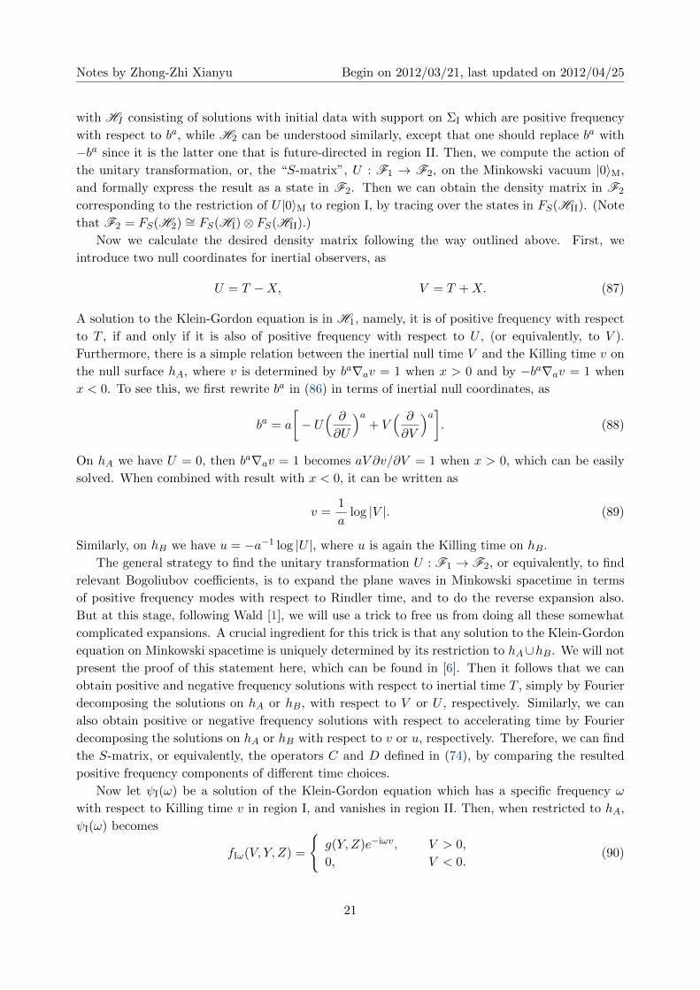
Killing field are shown in Fig. 1, from which we see that ba fails to be globally timelike. But it is

timelike within the region I given by |X| > T . In addition, Region I is also globally hyperbolic.

Therefore we may view the Region I as an independent spacetime being globally hyperbolic and

stationary, and construct quantum field theories there. By the construction described in Subsection

3.3, there is a natural concept of particles in this stationary spacetime. In particular, the vacuum

state associated with this construction unambiguously is called the Rindler vacuum.

III

III

IV

ShA

hB

SISII

U V

Figure 1: Unruh Effect.

From the viewpoint of an inertial observer with coordinates (T,X, Y, Z), particles at rest in

frames with ba-Killing time undergoes a motion of uniform acceleration, with different acceleration

for different orbits. For the object along the orbit baba = −1, namely X2 = T 2 + a−2, it is easy

to show that its 3-velocity is w = aT√

1 + a2T 2, and the spatial component of its 4-velocity if

γw = aT , with γ ≡ 1/√

1− w2 =√

1 + a2T 2. Thus its acceleration is simply a.

Now we can construct quantum field theories in two different ways. One is associated with

inertial frame with global coordinates (T,X, Y, Z), the other is constructed with the time transla-

tion generated by Killing field ba in region I. The problem we want to address is that what does

the vacuum state of inertial construction, which we will called Minkowski vacuum, look like from

the viewpoint of an accelerated observer? More precisely, we would like to express the Minkowski

vacuum state |0〉M in terms of states in Fock space associated with accelerated observers, namely,

with Killing time v satisfying ba∇av = 1.

For this purpose, we first construct a new quantum state space F2 = FS(H2) associated with

accelerated observers, besides the inertial one which we denote as F1 = FS(H1). That is, H2

consists of solutions of positive frequency with respect to the Killing time v, while H1 consists

of those with respect to the inertial time T . Now, let Σ be a Cauchy surface of the Minkowski

spacetime passing through the bifurcation surface S, and let ΣI and ΣII be the portions of Σ in

region I and region II, respectively. Then, H2 can be obtained by the direct sum H2 = HI ⊕HII,

20


with HI consisting of solutions with initial data with support on ΣI which are positive frequency

with respect to ba, while H2 can be understood similarly, except that one should replace ba with

−ba since it is the latter one that is future-directed in region II. Then, we compute the action of

the unitary transformation, or, the “S-matrix”, U : F1 → F2, on the Minkowski vacuum |0〉M,

and formally express the result as a state in F2. Then we can obtain the density matrix in F2

corresponding to the restriction of U |0〉M to region I, by tracing over the states in FS(HII). (Note

that F2 = FS(H2) ∼= FS(HI)⊗ FS(HII).)

Now we calculate the desired density matrix following the way outlined above. First, we

introduce two null coordinates for inertial observers, as

U = T −X, V = T +X. (87)

A solution to the Klein-Gordon equation is in H1, namely, it is of positive frequency with respect

to T , if and only if it is also of positive frequency with respect to U , (or equivalently, to V ).

Furthermore, there is a simple relation between the inertial null time V and the Killing time v on

the null surface hA, where v is determined by ba∇av = 1 when x > 0 and by −ba∇av = 1 when

x < 0. To see this, we first rewrite ba in (86) in terms of inertial null coordinates, as

ba = a

[− U

( ∂

∂U

)a+ V

( ∂

∂V

)a]. (88)

On hA we have U = 0, then ba∇av = 1 becomes aV ∂v/∂V = 1 when x > 0, which can be easily

solved. When combined with result with x < 0, it can be written as

v =1

alog |V |. (89)

Similarly, on hB we have u = −a−1 log |U |, where u is again the Killing time on hB.

The general strategy to find the unitary transformation U : F1 → F2, or equivalently, to find

relevant Bogoliubov coefficients, is to expand the plane waves in Minkowski spacetime in terms

of positive frequency modes with respect to Rindler time, and to do the reverse expansion also.

But at this stage, following Wald [1], we will use a trick to free us from doing all these somewhat

complicated expansions. A crucial ingredient for this trick is that any solution to the Klein-Gordon

equation on Minkowski spacetime is uniquely determined by its restriction to hA∪hB. We will not

present the proof of this statement here, which can be found in [6]. Then it follows that we can

obtain positive and negative frequency solutions with respect to inertial time T , simply by Fourier

decomposing the solutions on hA or hB, with respect to V or U , respectively. Similarly, we can

also obtain positive or negative frequency solutions with respect to accelerating time by Fourier

decomposing the solutions on hA or hB with respect to v or u, respectively. Therefore, we can find

the S-matrix, or equivalently, the operators C and D defined in (74), by comparing the resulted

positive frequency components of different time choices.

Now let ψI(ω) be a solution of the Klein-Gordon equation which has a specific frequency ω

with respect to Killing time v in region I, and vanishes in region II. Then, when restricted to hA,

ψI(ω) becomes

fIω(V, Y, Z) =

g(Y, Z)e−iωv, V > 0,

0, V < 0.(90)

21


We want to resolute this function into Fourier modes with respect to inertial null time V . Let us

denote the frequency variable associated with V by σ, then the Fourier modes with frequency σ is

given by

fIω =1√2π

∫ ∞−∞

dV fIω(V, Y, Z)eiσV =1√2πg(Y,Z)I(σ), (91)

with

I(σ) =

∫ ∞0

dV e−i(ω/a) log V eiσV . (92)

In the same way, we can consider the solutions in region II. But these solutions can also be obtained

from the “wedge reflection” isometry (T,X, Y, Z) → (−T,−X,Y, Z). Under this transformation,

solutions fIω transforms to fIIω, which is of mono frequency on hA when x < 0 and vanishes on

hA when x > 0. That is, we have

fIIω(V, Y, Z) =

0, V > 0,

g(Y,Z)e−iωv, V < 0.(93)

This function can also be decomposed into modes with respect to V , as

˜fIIω =1√2πg(Y, Z)

∫ 0

−∞dV e−i(ω/a) log |V |eiσV

=1√2πg(Y, Z)

∫ ∞0

dV e−i(ω/a) log |V |e−iσV =1√2πg(Y,Z)I(−σ). (94)

Then we see immediately that

˜fIIω(σ, Y, Z) = fIω(−σ, Y, Z). (95)

To relate these modes with positive or negative modes with respect to inertial null time V , we

make use of the trick of symmetry analysis. Our claim is,

fIω(−σ, Y, Z) = −e−πω/afIω(σ, Y, Z), σ > 0. (96)

To prove this equation, we evaluate I(σ) for σ > 0 defined in (92), by making the substitution

V = iy and rotating y to the positive real axis. Here we put the branch cut of logarithm to the

negative real axis. Then, log V = log(iy) = log y + iπ/2, and

I(σ) = ieπω/2a∫ ∞

0dy e−i(ω/a) log ye−σy. (97)

To fine I(−σ), we make the substitution V = −iσ, and proceed in the same way, and this time we

have

I(−σ) = −ie−πω/2a∫ ∞

0dy e−i(ω/a) log ye−σy. (98)

Then (96) follows straightforwardly.

Now, we define two functions Fω F′ω on hA by

Fω = fIω + e−πω/afIIω, F ′ω = fIIω + e−πω/aψIω. (99)

22


We decompose Fω in terms of modes with respect to V . Then its negative frequency modes read:

Fω(−σ, Y, Z) = fIω(−σ, Y, Z) + e−πω/a ˜fIIω(−σ, Y, Z)

=− e−πω/afIω(σ, Y, Z) + e−πω/afIω(σ, Y, Z) = 0, (100)

where we have used (95) and (96). That is, Fω is a of pure positive frequency with respect to V .

In the same way, we can show that F ′ω is also of pure positive frequency. Now, definitions of the

operators C : H1 →H2 and D : H1 → H2, we have

CFω = fIω, DFω = e−πω/afIIω; CF ′ω = fIIω, DF ′ω = e−πω/afIω. (101)

Therefore,

DC−1fIω = e−πω/afIIω, DC−1fIIω = e−πω/afIω. (102)

Note that fIω and fIIω span HI and HII respectively, which means they span H2 = HI ⊕HII

together, thus we have completely determined the operator E = DC−1. Then according to (to be

added), the corresponding two particle state is given by

εab =∑i

e−πωi/a2f(aIωifb)IIωi

, (103)

which can be rewritten in Dirac notations as

U |0〉M =∏i

( ∞∑n=0

e−nπωi/a|ni〉I ⊗ |ni〉II)

(104)

This is the result of acting the unitary transformation U on the Minkowski vacuum state. Now we

take the tensor product of it and trace over FS(H2), to get

ρ = tr FS(H2)

∏i

∞∑n=0

e−2nπωi/a|ni〉I|ni〉II II〈ni|I〈ni|

=∏i

∞∑n=0

e−2nπωi/a|ni〉I I〈ni| (105)

This is exactly the thermal density matrix with temperature

T =a

2π, (106)

which is known as the Unruh effect.

We finish this subsection with some remarks.

4.2 Killing horizons

Now we are going to generalize the previous derivation of Unruh effect to curved spacetime.

Note that the derivation above depends essentially on the structure of four wedge-like regions.

Thus we will at first introduce the similar structure in curved spacetime, namely the so-called

“bifurcate Killing horizon”.

23


For illustration we firstly consider the case of 2d spacetime. We recall that an isometry is

defined to be a diffeomorphism of the spacetime (M , gab) that leaves the metric gab invariant, and

that a Killing vector field ξa is defined to be the generator of a one-parameter group of isometries.

It follows directly that ξa satisfies ∇(aξb) = 0. Another property of Killing field which is crucial

here is that it is uniquely determined over the spacetime manifold by its action (of a spacetime

function) on one point p ∈M together with its induced action on the tangent space Vp to p. Stated

equivalently, a Killing vector filed ξa on spacetime manifold M is uniquely specified by its value

ξa and the value of its derivative Fab ≡ ∇aξb = ∇[aξb] at one point. This result is most easily seen

from the fact that the Killing field ξa satisfies the following equation:

∇c∇aξb = −Rabcdχd. (107)

Then the statement above is justified by the uniqueness of the solution to this differential equation

once the initial condition is given.

Now, in 2d spacetime, suppose a Killing field ξa vanishes on the point p, ξa(p) = 0. then ξa

is totally determined by the antisymmetric tensor Fab = ∇aχb, which has only one independent

component in 2d. This single component is nothing but the coefficient of the Lie derivative of a

vector, namely, Lξva = F abξ

b. The vanishing of ξa(p) = 0 simply means that p is a fixed-point of

the one-parameter group of isometries, and the behavior of ξa within a small neighborhood of p is

determined by the signature of the spacetime metric. In Riemannian case, ξa is the generator of

rotations and its integration curves is a family of ellipses, while in Minkowskian case, xia generates

Lorentz boosts and its integration curves are hyperbolas, which has exactly the same structure as

shown in Fig. 1.

Similar things happen in n > 2 dimensions, if a Killing field ξa vanishes entirely over an (n−2)d

spacelike surface S. In Minkowskian case, the pair of hypersurfaces hA and hB generated by null

geodesics orthogonal to S is called a bifurcate Killing horizon. This bifurcate Killing horizon locally

divides the spacetime into four wedges as shown in Fig. 1.

Now we introduce the concept of surface gravity of an arbitrary Killing horizon. A Killing

horizon h associated with the Killing field χa is defined to be a null surface to which χa is normal.

Now, by definition we have χaχa = 0 on h, thus ∇b(χaχa) must be normal to h. Since χa itself is

also normal to h, then these two vectors must be proportional, namely, there exists a function κ

on h, namely the surface gravity of h, such that

∇b(χaχa) = −2κχb. (108)

The surface gravity can be represented in terms of the Killing field χa to be

κ2 = − 12 (∇aχb)(∇aχb), (109)

or,

κ = limp→h

a√−χaχa, (110)

where a is the magnitude of the proper acceleration of the orbits of χa in the region outside h

where ξa is timelike, and the limit is taken to approach the horizon. The name of “surface gravity”

can be understood in the asymptotically flat spacetime in which the Killing field χa approaches a

time translation at infinity. Then one can normalize χa such that χaχa → −1 at infinity. It follows

24


directly that√−χaχa is now the gravitational redshift factor, and (110) is simply the redshifted

proper acceleration of orbits of χa near the horizon, which is equivalent in the usual sense to the

concept of surface gravity.

A crucial property of the bifurcate Killing horizons is that the surface gravity κ is a constant

over the whole horizon. This can be proved in two steps. Firstly, the surface gravity κ is constant

along each orbit of χa on h, which can be directly seen by taking the Lie derivative of (108) with

respect to χa.

It can be shown that the event horizon of a stationary black hole must be a Killing horizon,

which in turn comprises a portion of a bifurcate Killing horizon, except in the “degenerating” case

of vanishing surface gravity.

References

[1] R. M. Wald, Quantum Field Theory in Curved Spacetime and Black Hole Thermodynamics,

The University of Chicago Press, 1994

[2] M. J. Gotay, “Functorial Geometric Quantization and Van Hove’s Theorem”, Int. J. Theor.

Phys. 19, 139.

[3] R. M. Wald, General Relativity, The University of Chicago Press, 1984.

[4] S. W. Hawking and G. F. R. Ellis, The Large Scale Structure of Space-Time, Cambridge

University Press, 1973.

[5] A. Ashtekar and A. Magnon, “Quantum Fields in Curved Space-Times”, Proc. Roy. Soc. Lond.

A 346, 375 (1975).

[6] B. S. Kay and R. M. Wald, “Theorems on the Uniqueness and Thermal Properties of a Sta-

tionary, Nonsingular, Quasifree States on Spacetimes with a Bifurcate Killing Horizon”, Phys.

Rep. 207, 49.

25

Reading Note on Quantum Field Theory in Curved Spacetime · Reading Note on Quantum Field Theory in...

Documents

Transcript of Reading Note on Quantum Field Theory in Curved Spacetime · Reading Note on Quantum Field Theory in...