RAVEN User Guide - Idaho National Laboratory
174
MANUAL INL/EXT-18-44465 Revision 0 Printed June 2018 RAVEN User Guide Andrea Alfonsi, Cristian Rabiti, Diego Mandelli, Joshua Cogliati, Congjian Wang, Paul W. Talbot, Daniel P. Maljovec Prepared by Idaho National Laboratory Idaho Falls, Idaho 83415 The Idaho National Laboratory is a multiprogram laboratory operated by Battelle Energy Alliance for the United States Department of Energy under DOE Idaho Operations Office. Contract DE-AC07-05ID14517. Approved for unlimited release.
Transcript of RAVEN User Guide - Idaho National Laboratory
MANUALINL/EXT-18-44465Revision 0Printed June 2018
RAVEN User Guide
Andrea Alfonsi, Cristian Rabiti, Diego Mandelli, Joshua Cogliati, Congjian Wang,Paul W. Talbot, Daniel P. Maljovec
Prepared byIdaho National LaboratoryIdaho Falls, Idaho 83415
The Idaho National Laboratory is a multiprogram laboratory operated byBattelle Energy Alliance for the United States Department of Energyunder DOE Idaho Operations Office. Contract DE-AC07-05ID14517.
Approved for unlimited release.

Issued by the Idaho National Laboratory, operated for the United States Department of Energyby Battelle Energy Alliance.
NOTICE: This report was prepared as an account of work sponsored by an agency of the UnitedStates Government. Neither the United States Government, nor any agency thereof, nor anyof their employees, nor any of their contractors, subcontractors, or their employees, make anywarranty, express or implied, or assume any legal liability or responsibility for the accuracy,completeness, or usefulness of any information, apparatus, product, or process disclosed, or rep-resent that its use would not infringe privately owned rights. Reference herein to any specificcommercial product, process, or service by trade name, trademark, manufacturer, or otherwise,does not necessarily constitute or imply its endorsement, recommendation, or favoring by theUnited States Government, any agency thereof, or any of their contractors or subcontractors.The views and opinions expressed herein do not necessarily state or reflect those of the UnitedStates Government, any agency thereof, or any of their contractors.
Printed in the United States of America. This report has been reproduced directly from the bestavailable copy.
DE
PA
RT
MENT OF EN
ER
GY
• • UN
IT
ED
STATES OFA
M
ER
IC
A
2
INL/EXT-18-44465Revision 0
Printed June 2018
RAVEN User Guide
Andrea AlfonsiCristian RabitiDiego MandelliJoshua CogliatiCongjian WangPaul W. Talbot
Daniel P. Maljovec
3

4

Contents1 Introduction . . . . . . . . . . . . . . . . . . . . . . . . . . . . . . . . . . . . . . . . . . . . . . . . . . . . . . . . . . . . . . . . . . . . . 7
1.1 Project Background . . . . . . . . . . . . . . . . . . . . . . . . . . . . . . . . . . . . . . . . . . . . . . . . . . 71.2 Acquiring and Installing RAVEN . . . . . . . . . . . . . . . . . . . . . . . . . . . . . . . . . . . . . . . 71.3 User Guide Formats . . . . . . . . . . . . . . . . . . . . . . . . . . . . . . . . . . . . . . . . . . . . . . . . . . 81.4 Capabilities of RAVEN . . . . . . . . . . . . . . . . . . . . . . . . . . . . . . . . . . . . . . . . . . . . . . . 91.5 Components of RAVEN . . . . . . . . . . . . . . . . . . . . . . . . . . . . . . . . . . . . . . . . . . . . . . . 111.6 Code Interfaces of RAVEN . . . . . . . . . . . . . . . . . . . . . . . . . . . . . . . . . . . . . . . . . . . . 131.7 User Guide Organization . . . . . . . . . . . . . . . . . . . . . . . . . . . . . . . . . . . . . . . . . . . . . . 15
2 RAVEN Tutorial . . . . . . . . . . . . . . . . . . . . . . . . . . . . . . . . . . . . . . . . . . . . . . . . . . . . . . . . . . . . . . . . . 162.1 Example Model: Analytic Bateman . . . . . . . . . . . . . . . . . . . . . . . . . . . . . . . . . . . . . . 162.2 Build RAVEN input: <SingleRun> . . . . . . . . . . . . . . . . . . . . . . . . . . . . . . . . . . . . 182.3 Build RAVEN Input: <IOStep> . . . . . . . . . . . . . . . . . . . . . . . . . . . . . . . . . . . . . . . 24
2.3.1 Perform input/output operations . . . . . . . . . . . . . . . . . . . . . . . . . . . . . . . . . . 252.3.2 Sub-plot and selectively printing. . . . . . . . . . . . . . . . . . . . . . . . . . . . . . . . . . 28
2.4 Build RAVEN Input: <MultiRun> . . . . . . . . . . . . . . . . . . . . . . . . . . . . . . . . . . . . . 312.5 Build RAVEN Input: <RomTrainer> . . . . . . . . . . . . . . . . . . . . . . . . . . . . . . . . . . 41
2.5.1 How to train and output a ROM? . . . . . . . . . . . . . . . . . . . . . . . . . . . . . . . . . 412.5.2 How to load and sample a ROM? . . . . . . . . . . . . . . . . . . . . . . . . . . . . . . . . . 45
2.6 Build RAVEN Input: <PostProcess> . . . . . . . . . . . . . . . . . . . . . . . . . . . . . . . . . 503 Forward Sampling Strategies . . . . . . . . . . . . . . . . . . . . . . . . . . . . . . . . . . . . . . . . . . . . . . . . . . . . . . 54
3.1 Monte-Carlo sampling through RAVEN . . . . . . . . . . . . . . . . . . . . . . . . . . . . . . . . . . 543.2 Grid sampling through RAVEN . . . . . . . . . . . . . . . . . . . . . . . . . . . . . . . . . . . . . . . . . 643.3 Stratified sampling through RAVEN . . . . . . . . . . . . . . . . . . . . . . . . . . . . . . . . . . . . . 733.4 Sparse Grid Collocation sampling through RAVEN . . . . . . . . . . . . . . . . . . . . . . . . . 83
4 Adaptive Sampling Strategies . . . . . . . . . . . . . . . . . . . . . . . . . . . . . . . . . . . . . . . . . . . . . . . . . . . . . 994.1 Limit Surface Search sampling through RAVEN . . . . . . . . . . . . . . . . . . . . . . . . . . . 99
5 Sampling from Restart . . . . . . . . . . . . . . . . . . . . . . . . . . . . . . . . . . . . . . . . . . . . . . . . . . . . . . . . . . . . 1106 Reduced Order Modeling through RAVEN . . . . . . . . . . . . . . . . . . . . . . . . . . . . . . . . . . . . . . . . . 1137 Statistical Analysis through RAVEN . . . . . . . . . . . . . . . . . . . . . . . . . . . . . . . . . . . . . . . . . . . . . . . 1298 Data Mining through RAVEN . . . . . . . . . . . . . . . . . . . . . . . . . . . . . . . . . . . . . . . . . . . . . . . . . . . . . 1379 Model Optimization . . . . . . . . . . . . . . . . . . . . . . . . . . . . . . . . . . . . . . . . . . . . . . . . . . . . . . . . . . . . . . 148
9.1 Introduction: The Optimizer Input . . . . . . . . . . . . . . . . . . . . . . . . . . . . . . . . . . . . . . . 1489.1.1 Models . . . . . . . . . . . . . . . . . . . . . . . . . . . . . . . . . . . . . . . . . . . . . . . . . . . . . . 1509.1.2 Data Objects . . . . . . . . . . . . . . . . . . . . . . . . . . . . . . . . . . . . . . . . . . . . . . . . . 1519.1.3 Out Streams . . . . . . . . . . . . . . . . . . . . . . . . . . . . . . . . . . . . . . . . . . . . . . . . . . 1519.1.4 Steps . . . . . . . . . . . . . . . . . . . . . . . . . . . . . . . . . . . . . . . . . . . . . . . . . . . . . . . 1529.1.5 Conclusion . . . . . . . . . . . . . . . . . . . . . . . . . . . . . . . . . . . . . . . . . . . . . . . . . . 152
9.2 Initial Conditions and Parallel Trajectories . . . . . . . . . . . . . . . . . . . . . . . . . . . . . . . . 1539.3 Summarizing Results . . . . . . . . . . . . . . . . . . . . . . . . . . . . . . . . . . . . . . . . . . . . . . . . . 1549.4 Adjusting Adaptive Steps . . . . . . . . . . . . . . . . . . . . . . . . . . . . . . . . . . . . . . . . . . . . . . 155
5

9.5 Denoising Stochastic Problems . . . . . . . . . . . . . . . . . . . . . . . . . . . . . . . . . . . . . . . . . 1579.6 Input Space Subdivision . . . . . . . . . . . . . . . . . . . . . . . . . . . . . . . . . . . . . . . . . . . . . . . 1599.7 Functional Constraints . . . . . . . . . . . . . . . . . . . . . . . . . . . . . . . . . . . . . . . . . . . . . . . . 160
10 EnsembleModel. . . . . . . . . . . . . . . . . . . . . . . . . . . . . . . . . . . . . . . . . . . . . . . . . . . . . . . . . . . . . . . . . . 16210.1 Introduction: The EnsembleModel . . . . . . . . . . . . . . . . . . . . . . . . . . . . . . . . . . . . . . 16210.2 Example: ballistics and impact . . . . . . . . . . . . . . . . . . . . . . . . . . . . . . . . . . . . . . . . . 162
10.2.1 DataObjects . . . . . . . . . . . . . . . . . . . . . . . . . . . . . . . . . . . . . . . . . . . . . . . . . . 16310.2.2 Files . . . . . . . . . . . . . . . . . . . . . . . . . . . . . . . . . . . . . . . . . . . . . . . . . . . . . . . . 16410.2.3 Models . . . . . . . . . . . . . . . . . . . . . . . . . . . . . . . . . . . . . . . . . . . . . . . . . . . . . . 16510.2.4 Steps . . . . . . . . . . . . . . . . . . . . . . . . . . . . . . . . . . . . . . . . . . . . . . . . . . . . . . . 166
10.3 ExternalModel in EnsembleModel . . . . . . . . . . . . . . . . . . . . . . . . . . . . . . . . . . . . . . 16710.3.1 Input Placeholder DataObject . . . . . . . . . . . . . . . . . . . . . . . . . . . . . . . . . . . . 16710.3.2 DataSet . . . . . . . . . . . . . . . . . . . . . . . . . . . . . . . . . . . . . . . . . . . . . . . . . . . . . 16810.3.3 Scalar Variables . . . . . . . . . . . . . . . . . . . . . . . . . . . . . . . . . . . . . . . . . . . . . . . 16810.3.4 Independent Variables . . . . . . . . . . . . . . . . . . . . . . . . . . . . . . . . . . . . . . . . . . 169
Appendices . . . . . . . . . . . . . . . . . . . . . . . . . . . . . . . . . . . . . . . . . . . . . . . . . . . . . . . . . . . . . . . . . . . . . . . . . 171A Document Version Information . . . . . . . . . . . . . . . . . . . . . . . . . . . . . . . . . . . . . . . . . . . . . . . . . . . . 171References . . . . . . . . . . . . . . . . . . . . . . . . . . . . . . . . . . . . . . . . . . . . . . . . . . . . . . . . . . . . . . . . . . . . . . . . . . 172
6
1 Introduction
1.1 Project Background
The development of RAVEN started in 2012 when, within the Nuclear Energy Advanced Modelingand Simulation (NEAMS) program [1], the need of a modern risk evaluation framework arose.RAVEN’s principal assignment is to provide the necessary software and algorithms in order toemploy the concepts developed by the Risk Informed Safety Margin Characterization (RISMC)Pathway. RISMC is one of the pathways defined within the Light Water Reactor Sustainability(LWRS) program [2].
The goal of the RISMC approach is the identification not only of the frequency of an eventwhich can potentially lead to system failure, but also the proximity (or lack thereof) to key safety-related events: the safety margin. Hence, the approach is interested in identifying and increasingthe safety margins related to those events. A safety margin is a numerical value quantifying theprobability that a safety metric (e.g. peak pressure in a pipe) is exceeded under certain conditions.Most of the capabilities, implemented having Reactor Excursion and Leak Analysis Program v.7(RELAP-7) as a principal focus, are easily deployable to other system codes. For this reason,several side activates have been employed (e.g. RELAP5-3D [3], any Multiphysics Object OrientedSimulation Environment-based App, etc.) or are currently ongoing for coupling RAVEN withseveral different software.
1.2 Acquiring and Installing RAVEN
RAVEN is supported on three separate computing platforms: Linux, OSX (Apple Macintosh), andMicrosoft Windows. Currently, RAVEN is open-source and downloadable from RAVEN GitHubrepository: https://github.com/idaholab/raven. New users should visit https://github.com/idaholab/raven/wiki or refer to the user manual [4] to get started withRAVEN. This typically involves the following steps:
• Download RAVENYou can download the source code of RAVEN from https://github.com/idaholab/raven.
• Install RAVEN dependenciesInstructions are available from https://github.com/idaholab/raven/wiki, orthe user manual [4].
• Install RAVENInstructions are available from https://github.com/idaholab/raven/wiki, orthe user manual [4].
7

• Run RAVENIf RAVEN is installed successfully, please run the regression tests to verify your installation:
./run_tests
Normally there are skipped tests because either some of the codes are not available, or someof the test are not currently working. The output will explain why each is skipped. If allthe tests pass, you are ready to run RAVEN. Now, open a terminal and use the followingcommand (replace <inputFileName.xml> with your RAVEN input file):
raven_framework <inputFileName.xml>
where the raven framework script can be found in the RAVEN folder. Alternatively, theDriver.py script contained in the folder “raven/framework” can be directly used:
python raven/framework/Driver.py <inputFileName.xml>
• Participate in RAVEN user communitiesJoin RAVEN mail lists to get help and updates of RAVEN: https://groups.google.com/forum/#!forum/inl-raven-users.
1.3 User Guide Formats
In order to highlight some parts of the user guide having a particular meaning (input structure,examples, terminal commands, etc.), specific formats have been used. This section provides theformats with a specific meaning:
• Python Coding:
class AClass():def aMethodImplementation(self):
pass
• RAVEN XML input example:
<MainXMLBlock>...<aXMLnode name='anObjectName' anAttribute='aValue'>
<aSubNode>body</aSubNode></aXMLnode><!-- This is commented block -->...
</MainXMLBlock>
8
• Bash Commands:
cd trunk/raven/./raven_libs_script.shcd ../../
1.4 Capabilities of RAVEN
RAVEN [5] [6] [7] [8] is a software framework that allows the user to perform parametric andstochastic analysis based on the response of complex system codes. The initial developmentwas designed to provide dynamic probabilistic risk analysis capabilities (DPRA) to the thermal-hydraulic code RELAP-7 [9], currently under development at Idaho National Laboratory (INL).Now, RAVEN is not only a framework to perform DPRA but it is a flexible and multi-purpose un-certainty quantification, regression analysis, probabilistic risk assessment, data analysis and modeloptimization platform. Depending on the tasks to be accomplished and on the probabilistic charac-terization of the problem, RAVEN perturbs (e.g., Monte-Carlo, Latin hypercube, reliability surfacesearch) the response of the system under consideration by altering its own parameters. The systemis modeled by third party software (e.g., RELAP5-3D, MAAP5, BISON, etc.) and accessible toRAVEN either directly (software coupling) or indirectly (via input/output files). The data gener-ated by the sampling process is analyzed using classical statistical and more advanced data miningapproaches. RAVEN also manages the parallel dispatching (i.e. both on desktop/workstation andlarge High Performance Computing machines) of the software representing the physical model.RAVEN heavily relies on artificial intelligence algorithms to construct surrogate models of com-plex physical systems in order to perform uncertainty quantification, reliability analysis (limit statesurface) and parametric studies.
The main capabilities of RAVEN, with brief descriptions, are summarized here, or one cancheck the Figure. 1. These capabilities may be used on their own or as building blocks to con-struct the sought workflow. In addition, RAVEN also provides some more sophisticated Ensemblealgorithms such as EnsembleForward, EnsembleModel to combine the existing capabilites.
• Sensitivity Analysis and Uncertainty Quantification: Sensitivity analysis is a mathemat-ical tool that can be used to identify the key sources of uncertainties. Uncertainty quantifi-cation is a process by which probabilistic information about system responses can be com-puted according to specified input parameter probability distributions. Available approachesin RAVEN include Monte Carlo, Grid, Stratified (Latin hypercube), Sparse Grid Collo-cation, Sobol, Adaptive Sparse Grid, Adaptive Sobol and BasicStatistics.
• Design of Experiments: The design of experiments (DOE) is a powerful tool that can beused to explore the parameter space at a variety of experimental situations. It can be used
9
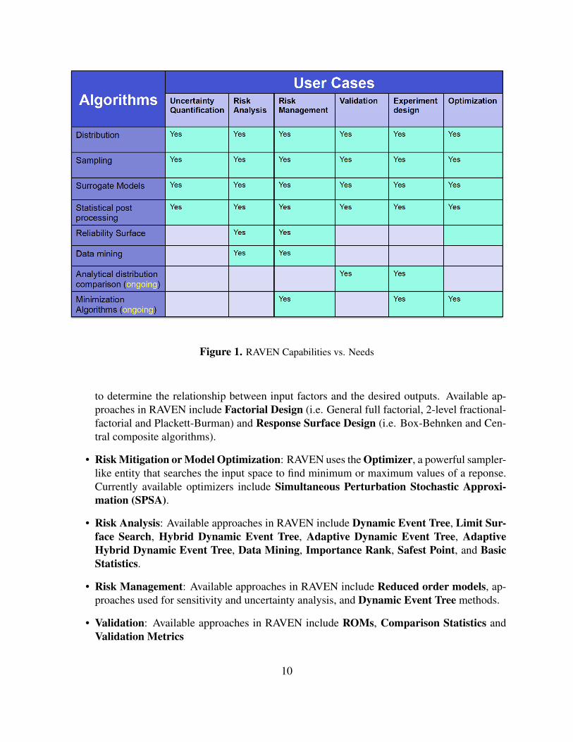
Figure 1. RAVEN Capabilities vs. Needs
to determine the relationship between input factors and the desired outputs. Available ap-proaches in RAVEN include Factorial Design (i.e. General full factorial, 2-level fractional-factorial and Plackett-Burman) and Response Surface Design (i.e. Box-Behnken and Cen-tral composite algorithms).
• Risk Mitigation or Model Optimization: RAVEN uses the Optimizer, a powerful sampler-like entity that searches the input space to find minimum or maximum values of a reponse.Currently available optimizers include Simultaneous Perturbation Stochastic Approxi-mation (SPSA).
• Risk Analysis: Available approaches in RAVEN include Dynamic Event Tree, Limit Sur-face Search, Hybrid Dynamic Event Tree, Adaptive Dynamic Event Tree, AdaptiveHybrid Dynamic Event Tree, Data Mining, Importance Rank, Safest Point, and BasicStatistics.
• Risk Management: Available approaches in RAVEN include Reduced order models, ap-proaches used for sensitivity and uncertainty analysis, and Dynamic Event Tree methods.
• Validation: Available approaches in RAVEN include ROMs, Comparison Statistics andValidation Metrics
10

In addition, RAVEN includes a number of related advanced capabilities. Surrogate or Re-duced order models (ROMs) are mathematical model trained to predict a response of interest ofa physical system. Typically, ROMs trade speed for accuracy representing a faster, rough estimateof the underlying systems. They can be used to explore the input parameter space for optimiza-tion or sensitivity and uncertainty studies. Ensemble Model is able to combine Codes, ExternalModels and ROMs. It is intended to create a chain of models whose execution order is determinedby the input/output relationships among them. If the relationships among the models evolve in anon-linear system, a Picard’s iteration scheme is employed.
1.5 Components of RAVEN
The RAVEN code does not have a fixed calculation flow, since all of its basic objects can becombined in order to create a user-defined calculation flow. Thus, its input, eXtensible MarkupLanguage (XML) format, is organized in different XML blocks, each with a different functionality.For more information about XML, please click on the link: XML tutorial.The main input blocks are as follows:
• <Simulation>: The root node containing the entire input, all of the following blocks fitinside the Simulation block.
• <RunInfo>: Specifies the calculation settings (number of parallel simulations, etc.).
• <Files>: Specifies the files to be used in the calculation.
• <Distributions>: Defines distributions needed for describing parameters, etc.
• <Samplers>: Sets up the strategies used for exploring an uncertain domain.
• <DataObjects>: Specifies internal data objects used by RAVEN.
• <Databases>: Lists the HDF5 databases used as input/output to a RAVEN run.
• <OutStreams>: Visualization and Printing system block.
• <Models>: Specifies codes, ROMs, post-processing analysis, etc.
• <Functions>: Details interfaces to external user-defined functions and modules the userwill be building and/or running.
• <VariableGroups>: Creates a collection of variables.
• <Optimizers>: Performs the driving of a specific goal function over the model for valueoptimization.
• <Metrics>: Calculate the distance values among points and histories.
11

• <Steps>: Combines other blocks to detail a step in the RAVEN workflow including I/Oand computations to be performed.
Each of these components are explained in dedicated sections of the user manual [4], and canbe used as building blocks to construct certain calculation flow, as shown in Figure. 2. In this guide,we will only show how to use these components to build the analysis flow, and we recommend theuser to check the user manual [4] for the detailed descriptions.
Figure 2. RAVEN structures
In addition, RAVEN allows the user to load any external input file that contains the requiredXML nodes into the RAVEN main input file, and provide the standard XML comments, using<!--and -->. For example, one can use the following template to load the <Distributions> fromfile ‘Distributions.xml’.
<Simulation verbosity='all'>...<!-- An Example Comment --><Steps verbosity='debug'>
...</Steps>...<ExternalXML node='Distributions'
xmlToLoad='path_to_folder/Distributions.xml'/>
12
...</Simulation>
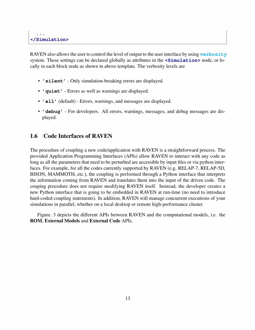
RAVEN also allows the user to control the level of output to the user interface by using verbositysystem. These settings can be declared globally as attributes in the <Simulation> node, or lo-cally in each block node as shown in above template. The verbosity levels are
• ’silent’ - Only simulation-breaking errors are displayed.
• ’quiet’ - Errors as well as warnings are displayed.
• ’all’ (default) - Errors, warnings, and messages are displayed.
• ’debug’ - For developers. All errors, warnings, messages, and debug messages are dis-played.
1.6 Code Interfaces of RAVEN
The procedure of coupling a new code/application with RAVEN is a straightforward process. Theprovided Application Programming Interfaces (APIs) allow RAVEN to interact with any code aslong as all the parameters that need to be perturbed are accessible by input files or via python inter-faces. For example, for all the codes currently supported by RAVEN (e.g. RELAP-7, RELAP-5D,BISON, MAMMOTH, etc.), the coupling is performed through a Python interface that interpretsthe information coming from RAVEN and translates them into the input of the driven code. Thecouping procedure does not require modifying RAVEN itself. Instread, the developer creates anew Python interface that is going to be embedded in RAVEN at run-time (no need to introducehard-coded coupling statements). In addition, RAVEN will manage concurrent executions of yoursimulations in parallel, whether on a local desktop or remote high-performance cluster.
Figure. 3 depicts the different APIs between RAVEN and the computational models, i.e. theROM, External Models and External Code APIs.
13

Figure 3. RAVEN Application Programming Interfaces
14

1.7 User Guide Organization
The goal of this document is to provide a set of detailed examples that can help the user to becomefamiliar with the RAVEN code. RAVEN is capable of investigating system response and exploreinput space using various sampling schemes such as Monte Carlo, grid, or Latin Hypercube. How-ever, RAVEN strength lies in its system feature discovery capabilities such as: constructing limitsurfaces, separating regions of the input space leading to system failure, and using dynamic super-vised learning techniques. New users should consult the RAVEN Tutorial to get started.
• RAVEN Tutorial: section 2
• Sampling Strategies: section 3 and section 4
• Restart: section 5
• Reduced Order Modeling: section 6
• Risk Analysis: section 7
• Data Mining: section 8
• Model Optimization: section 9
15

2 RAVEN Tutorial
2.1 Example Model: Analytic Bateman
This section is intended for the new users to familiarize them with how to perform their studiesthrough RAVEN. A simple example, conventionally called AnalyticBateman, has been developed.It solves a system of ordinary differential equations (ODEs), of the form:
dX
dt= S− L
X(t = 0) = X0
(1)
where:
• X0, initial conditions
• S, source terms
• L, loss terms
For example, this code is able to solve a system of two ODEs as follows:
dx1dt
= φ(t)× σx1 − λx1 × x1(t)
dx2dt
= φ(t)× σx2 − λx2 × x2(t) + x1(t)× λx1
x1(t = 0) = x01x2(t = 0) = 0.0
(2)
The input of the AnalyticBateman code is in XML format. For example, the following is thereference input for a system of 4 Ordinary Differential Equations (ODEs) that is going to be usedfor as an example in this guide. All the files required for this system are located at “raven/test-s/framework/user guide/physicalCode”.
raven/tests/framework/user guide/physicalCode/analyticalbateman/Input.xml
<AnalyticalBateman><totalTime>10</totalTime>
<powerHistory>1 1 1</powerHistory>
<flux>10000 10000 10000</flux>
16

<stepDays>0 100 200 300</stepDays>
<timeSteps>10 10 10</timeSteps>
<nuclides><A>
<equationType>N1</equationType><initialMass>1.0</initialMass><decayConstant>0</decayConstant><sigma>1</sigma><ANumber>230</ANumber>
</A><B>
<equationType>N2</equationType><initialMass>1.0</initialMass><decayConstant>0.00000005</decayConstant><sigma>10</sigma><ANumber>200</ANumber>
</B><C>
<equationType>N3</equationType><initialMass>1.0</initialMass><decayConstant>0.000000005</decayConstant><sigma>45</sigma><ANumber>150</ANumber>
</C><D>
<equationType>N4</equationType><initialMass>1.0</initialMass><decayConstant>0.00000008</decayConstant><sigma>3</sigma><ANumber>100</ANumber>
</D></nuclides>
</AnalyticalBateman>
The code outputs the time evolution of the 4 variables (A,B,C,D) in a CSV file, producing thefollowing output:
17
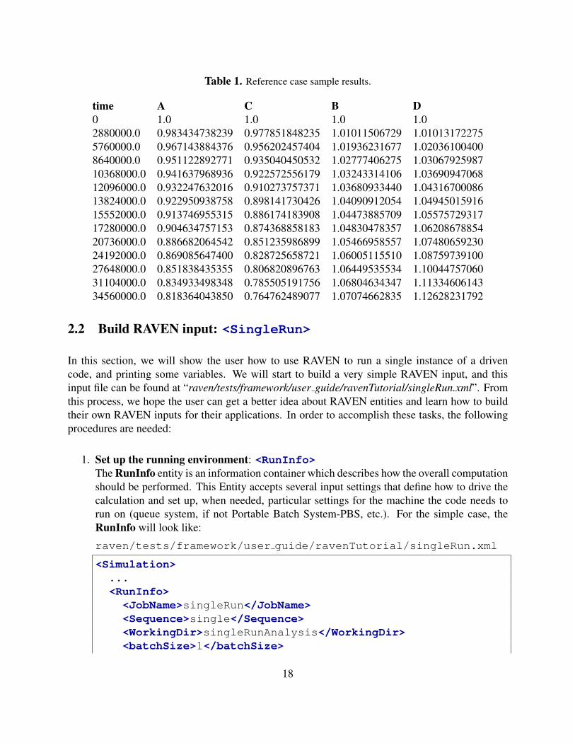
Table 1. Reference case sample results.
time A C B D0 1.0 1.0 1.0 1.02880000.0 0.983434738239 0.977851848235 1.01011506729 1.010131722755760000.0 0.967143884376 0.956202457404 1.01936231677 1.020361004008640000.0 0.951122892771 0.935040450532 1.02777406275 1.0306792598710368000.0 0.941637968936 0.922572556179 1.03243314106 1.0369094706812096000.0 0.932247632016 0.910273757371 1.03680933440 1.0431670008613824000.0 0.922950938758 0.898141730426 1.04090912054 1.0494501591615552000.0 0.913746955315 0.886174183908 1.04473885709 1.0557572931717280000.0 0.904634757153 0.874368858183 1.04830478357 1.0620867885420736000.0 0.886682064542 0.851235986899 1.05466958557 1.0748065923024192000.0 0.869085647400 0.828725658721 1.06005115510 1.0875973910027648000.0 0.851838435355 0.806820896763 1.06449535534 1.1004475706031104000.0 0.834933498348 0.785505191756 1.06804634347 1.1133460614334560000.0 0.818364043850 0.764762489077 1.07074662835 1.12628231792
2.2 Build RAVEN input: <SingleRun>
In this section, we will show the user how to use RAVEN to run a single instance of a drivencode, and printing some variables. We will start to build a very simple RAVEN input, and thisinput file can be found at “raven/tests/framework/user guide/ravenTutorial/singleRun.xml”. Fromthis process, we hope the user can get a better idea about RAVEN entities and learn how to buildtheir own RAVEN inputs for their applications. In order to accomplish these tasks, the followingprocedures are needed:
1. Set up the running environment: <RunInfo>The RunInfo entity is an information container which describes how the overall computationshould be performed. This Entity accepts several input settings that define how to drive thecalculation and set up, when needed, particular settings for the machine the code needs torun on (queue system, if not Portable Batch System-PBS, etc.). For the simple case, theRunInfo will look like:
raven/tests/framework/user guide/ravenTutorial/singleRun.xml
<Simulation>...<RunInfo>
<JobName>singleRun</JobName><Sequence>single</Sequence><WorkingDir>singleRunAnalysis</WorkingDir><batchSize>1</batchSize>
18
</RunInfo>...
</Simulation>
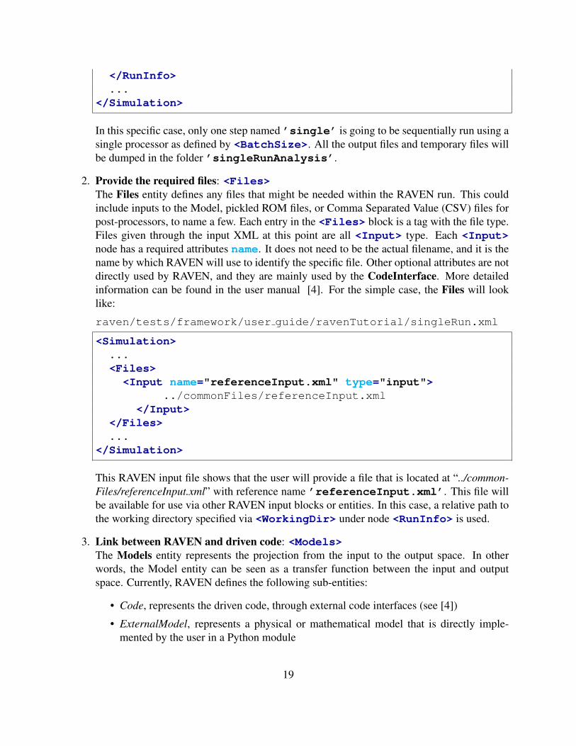
In this specific case, only one step named ’single’ is going to be sequentially run using asingle processor as defined by <BatchSize>. All the output files and temporary files willbe dumped in the folder ’singleRunAnalysis’.
2. Provide the required files: <Files>The Files entity defines any files that might be needed within the RAVEN run. This couldinclude inputs to the Model, pickled ROM files, or Comma Separated Value (CSV) files forpost-processors, to name a few. Each entry in the <Files> block is a tag with the file type.Files given through the input XML at this point are all <Input> type. Each <Input>node has a required attributes name. It does not need to be the actual filename, and it is thename by which RAVEN will use to identify the specific file. Other optional attributes are notdirectly used by RAVEN, and they are mainly used by the CodeInterface. More detailedinformation can be found in the user manual [4]. For the simple case, the Files will looklike:
raven/tests/framework/user guide/ravenTutorial/singleRun.xml
<Simulation>...<Files>
<Input name="referenceInput.xml" type="input">../commonFiles/referenceInput.xml
</Input></Files>...
</Simulation>
This RAVEN input file shows that the user will provide a file that is located at “../common-Files/referenceInput.xml” with reference name ’referenceInput.xml’. This file willbe available for use via other RAVEN input blocks or entities. In this case, a relative path tothe working directory specified via <WorkingDir> under node <RunInfo> is used.
3. Link between RAVEN and driven code: <Models>The Models entity represents the projection from the input to the output space. In otherwords, the Model entity can be seen as a transfer function between the input and outputspace. Currently, RAVEN defines the following sub-entities:
• Code, represents the driven code, through external code interfaces (see [4])
• ExternalModel, represents a physical or mathematical model that is directly imple-mented by the user in a Python module
19

• ROM, represents the Reduced Order Model, interfaced with several algorithms• HybridModel, automatic/smart Entity to automatically choose between a ROM (or a
set of them) and an High-Fidelity Model (e.g. ExternalModel, Code)• PostProcessor, is used to perform action on data, such as computation of statistical
moments, correlation matrices, etc.
For simplicity, only Code is used here for the demonstration, and the input block looks like:
raven/tests/framework/user guide/ravenTutorial/singleRun.xml
<Simulation>...<Models>
<Code name="testModel" subType="GenericCode"><executable>
../physicalCode/analyticalbateman/AnalyticalDplMain.py</executable><clargs arg="python" type="prepend" /><clargs arg="" extension=".xml" type="input" /><clargs arg=" " extension=".csv" type="output" />
</Code></Models>...
</Simulation>
As shown in the <Models> block, the subnodes defined for <Code> is equivalent to:
python ../physicalCode/analyticalbateman/AnalyticalDplMain.py
with the requirement of extensions of input and output files, as defined via <clargs>, to be’.xml’ and ’.csv’, respectively. In this case, the GenericCode interface is employed.This interface is meant to handle a wide variety of generic codes that take straightforwardinput files and produce CSV files. Note: If a code contains cross-dependent data, the genericinterface is not applicable. For more detailed information, the user can refer to sectionExisting Interface of the user manual [4].
4. Container of input and output data: <DataObjects>The DataObjects system is a container of data objects of various types that can be con-structed during the execution of desired calculation flow. These data objects can be used asinput or output for a particular Model Entity. Currently RAVEN supports the following datatypes, each with a particular conceptual meaning:
• PointSet is a collection of individual objects, each describing the state of the system ata certain point (e.g. in time). It can be considered a mapping between multiple sets ofparameters in the input space and the resulting sets of outcomes in the output space ata particular point (e.g., in time).
20
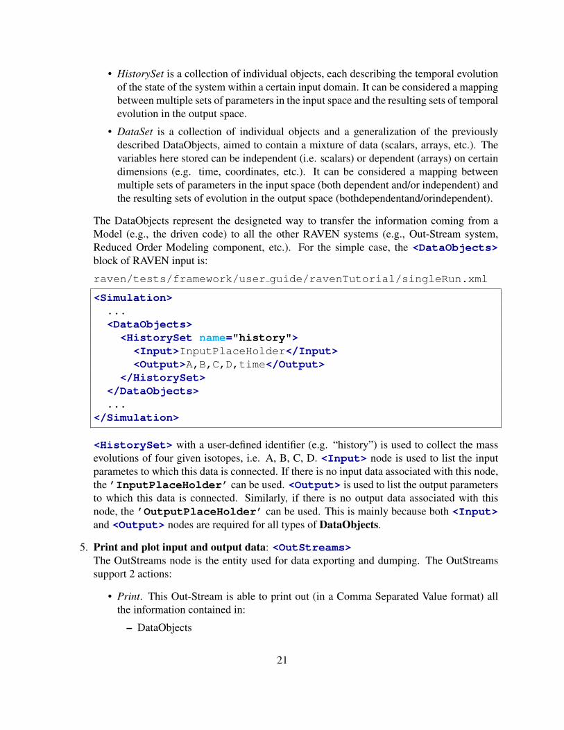
• HistorySet is a collection of individual objects, each describing the temporal evolutionof the state of the system within a certain input domain. It can be considered a mappingbetween multiple sets of parameters in the input space and the resulting sets of temporalevolution in the output space.
• DataSet is a collection of individual objects and a generalization of the previouslydescribed DataObjects, aimed to contain a mixture of data (scalars, arrays, etc.). Thevariables here stored can be independent (i.e. scalars) or dependent (arrays) on certaindimensions (e.g. time, coordinates, etc.). It can be considered a mapping betweenmultiple sets of parameters in the input space (both dependent and/or independent) andthe resulting sets of evolution in the output space (bothdependentand/orindependent).
The DataObjects represent the designeted way to transfer the information coming from aModel (e.g., the driven code) to all the other RAVEN systems (e.g., Out-Stream system,Reduced Order Modeling component, etc.). For the simple case, the <DataObjects>block of RAVEN input is:
raven/tests/framework/user guide/ravenTutorial/singleRun.xml
<Simulation>...<DataObjects>
<HistorySet name="history"><Input>InputPlaceHolder</Input><Output>A,B,C,D,time</Output>
</HistorySet></DataObjects>...
</Simulation>
<HistorySet> with a user-defined identifier (e.g. “history”) is used to collect the massevolutions of four given isotopes, i.e. A, B, C, D. <Input> node is used to list the inputparametes to which this data is connected. If there is no input data associated with this node,the ’InputPlaceHolder’ can be used. <Output> is used to list the output parametersto which this data is connected. Similarly, if there is no output data associated with thisnode, the ’OutputPlaceHolder’ can be used. This is mainly because both <Input>and <Output> nodes are required for all types of DataObjects.
5. Print and plot input and output data: <OutStreams>The OutStreams node is the entity used for data exporting and dumping. The OutStreamssupport 2 actions:
• Print. This Out-Stream is able to print out (in a Comma Separated Value format) allthe information contained in:
– DataObjects
21

– Reduced Order Models.
• Plot. This Out-Stream is able to plot 2-Dimensional, 3-Dimensional, 4-Dimensional(using color mapping) and 5-Dimensional (using marker size). Several types of plotare available, such as scatter, line, surfaces, histograms, pseudo-colors, contours, etc.
In this case, a simple <OutStreams> is used to output the mass evolutions of all fourmodel variables into a CSV file with the name prefix “print history”.
raven/tests/framework/user guide/ravenTutorial/singleRun.xml
<Simulation>...<OutStreams>
<Print name="print_history"><type>csv</type><source>history</source>
</Print></OutStreams>...
</Simulation>
6. Control of executions: <Steps>The Steps entity is used to create a peculiar analysis flow via combining together differentRAVEN entities. It is the location where all the defined entities get finally linked in order toperform a combined action on a certain Model. In order to perform this linking, each entitydefined in the Step needs to “play” a role:
• Input represents the input of the step. The allowable input objects depend on the typeof Model in this step.
• Model represents a physical or mathematical system or behavior. The object used inthis role defines the allowable types of inputs and outputs usable in this step.
• Output defines where to collect the results of an action performed by the Model. It isgenerally one of the following types: DataObjects, Databases, or OutStreams.
• Sampler defines the sampling strategy to be used to probe the model. Note: When asampling strategy is employed, the ”variables” defined in the <variable> blocks aregoing to be directly placed in the output objects of type DataObjects and Databases.
• Function is an extremely importance role. It introduces the capability to perform pre orpost processing of model inputs and outputs. Its specific behavior depends on the stepis using it.
• ROM defines an acceleration reduced order model to use for a step.
• SolutionExport, represents the container of the eventual output of a step. It is the entitythat is used to export the solution of a Sampler or post-processors.
22

Currently, RAVEN supports the following types of <Steps>:
• SingleRun, perform a single run of a model
• MultiRun, perform multiple runs of a model
• RomTrainer, perform the training of a Reduced Order Model (ROM)
• PostProcess, post-process data or manipulate RAVEN entities
• IOStep, step aimed to perform multiple actions:
– construct/update a Database from a DataObjects and vice-versa– construct/update a Database or a DataObjects object from CSV files– stream the content of a Database or a DataObjects out through an OutStream– store/retrieve a ROM to/from an external File using Pickle module of Python
For this example, the <SingleRun> is used to assemble a calculation flow, i.e. perform asingle action of a model.
raven/tests/framework/user guide/ravenTutorial/singleRun.xml
<Simulation>...<Steps><SingleRun name="single"><Input class="Files" type="input">referenceInput.xml</Input><Model class="Models" type="Code">testModel</Model><Output class="DataObjects"
type="HistorySet">history</Output><Output class="OutStreams"
type="Print">print_history</Output></SingleRun>
</Steps>...
</Simulation>
The code “testModel” will be executed once, and the outputs will be collected into a ’DataObjects’of type HistorySet. In addition, ’OutStreams’ is used to print the output data into a CSVfile.
The core of the RAVEN calculation flow is the Steps system. The Steps is in charge of assem-bling different entities in RAVEN in order to perform a task defined by the kind of step being used(see Figure. 4).
23
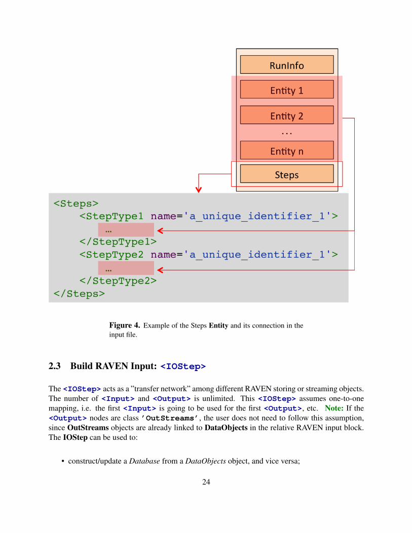
Figure 4. Example of the Steps Entity and its connection in theinput file.
2.3 Build RAVEN Input: <IOStep>
The <IOStep> acts as a ”transfer network” among different RAVEN storing or streaming objects.The number of <Input> and <Output> is unlimited. This <IOStep> assumes one-to-onemapping, i.e. the first <Input> is going to be used for the first <Output>, etc. Note: If the<Output> nodes are class ’OutStreams’, the user does not need to follow this assumption,since OutStreams objects are already linked to DataObjects in the relative RAVEN input block.The IOStep can be used to:
• construct/update a Database from a DataObjects object, and vice versa;
24
• construct/update a DataObject from a CSV file contained in a directory;
• construct/update a Database or a DataObjects object from CSV files contained in a directory;
• stream the content of a Database or a DataObjects out through an OutStream object;
• store/retrieve a ROM to/from an external File using Pickle module of Python.
The last function can be used to create and store mathematical model of fast solution trained to pre-dict a response of interest of a physical system. This model can be recovered in other simulationsor used to evaluate the response of a physical system in a Python program by the implementing ofthe Pickle module.
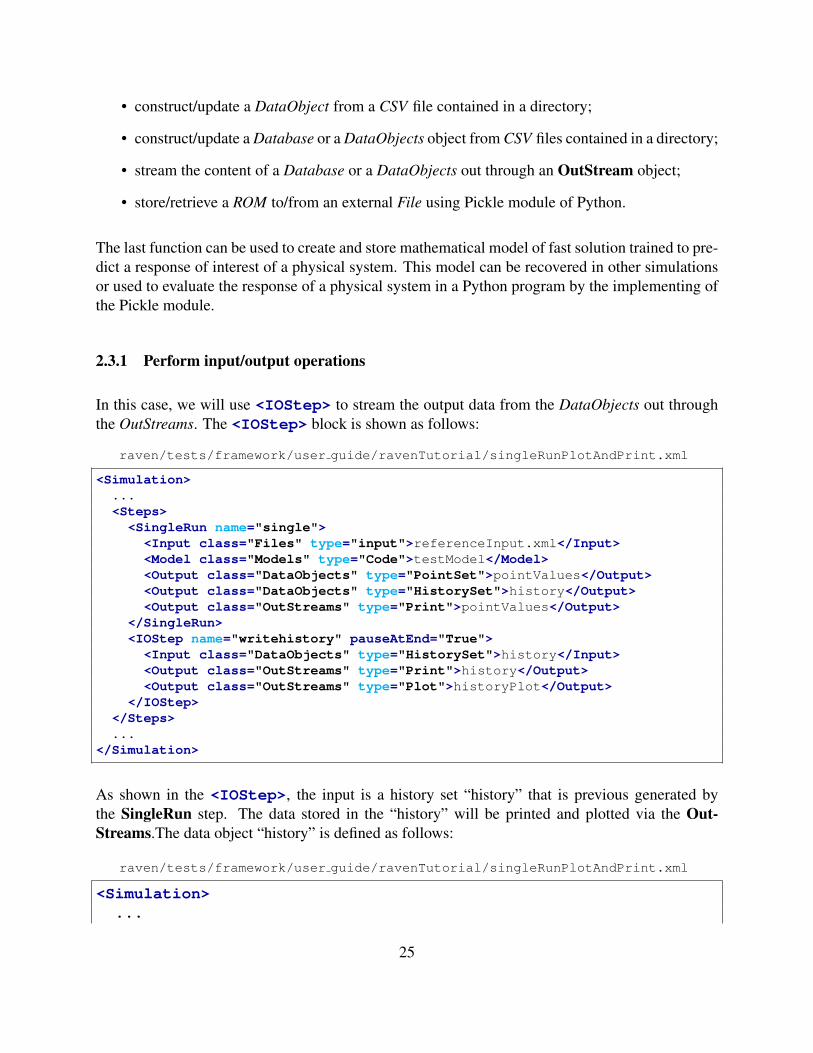
2.3.1 Perform input/output operations
In this case, we will use <IOStep> to stream the output data from the DataObjects out throughthe OutStreams. The <IOStep> block is shown as follows:
raven/tests/framework/user guide/ravenTutorial/singleRunPlotAndPrint.xml
<Simulation>...<Steps>
<SingleRun name="single"><Input class="Files" type="input">referenceInput.xml</Input><Model class="Models" type="Code">testModel</Model><Output class="DataObjects" type="PointSet">pointValues</Output><Output class="DataObjects" type="HistorySet">history</Output><Output class="OutStreams" type="Print">pointValues</Output>
</SingleRun><IOStep name="writehistory" pauseAtEnd="True"><Input class="DataObjects" type="HistorySet">history</Input><Output class="OutStreams" type="Print">history</Output><Output class="OutStreams" type="Plot">historyPlot</Output>
</IOStep></Steps>...
</Simulation>
As shown in the <IOStep>, the input is a history set “history” that is previous generated bythe SingleRun step. The data stored in the “history” will be printed and plotted via the Out-Streams.The data object “history” is defined as follows:
raven/tests/framework/user guide/ravenTutorial/singleRunPlotAndPrint.xml
<Simulation>...
25
<DataObjects><PointSet name="pointValues">
<Input>InputPlaceHolder</Input><Output>A,B,C,D</Output>
</PointSet><HistorySet name="history">
<Input>InputPlaceHolder</Input><Output>A,B,C,D,time</Output>
</HistorySet></DataObjects>...
</Simulation>
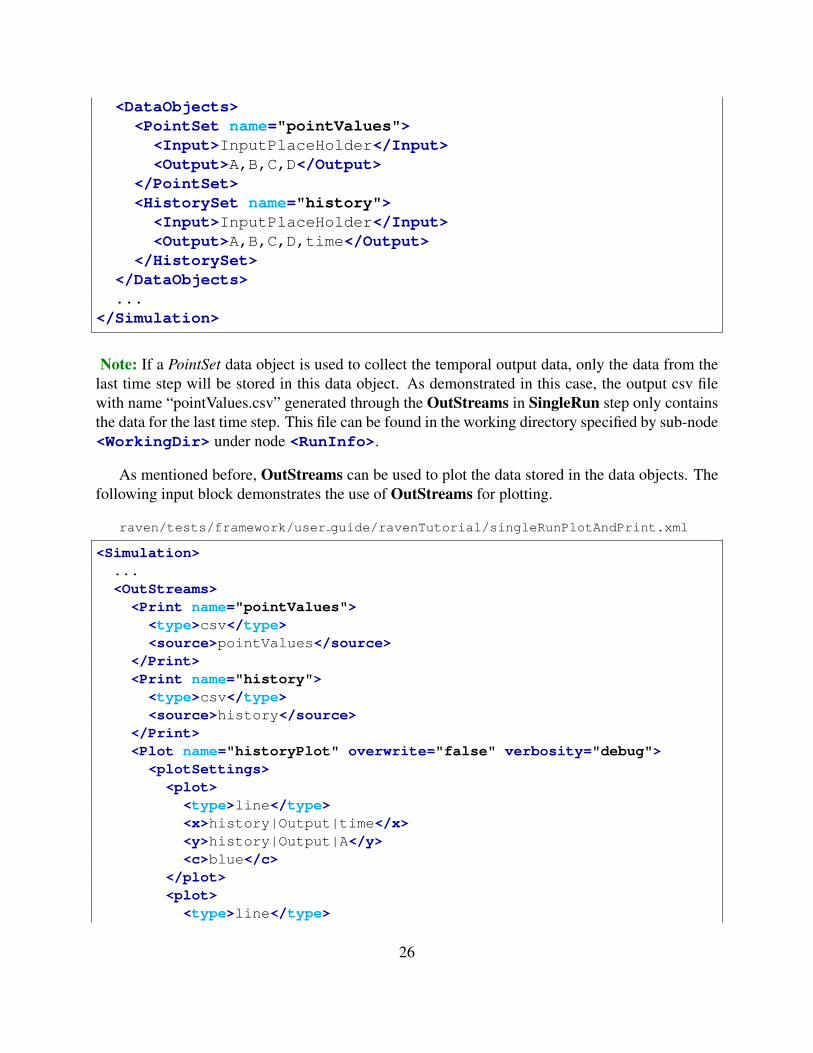
Note: If a PointSet data object is used to collect the temporal output data, only the data from thelast time step will be stored in this data object. As demonstrated in this case, the output csv filewith name “pointValues.csv” generated through the OutStreams in SingleRun step only containsthe data for the last time step. This file can be found in the working directory specified by sub-node<WorkingDir> under node <RunInfo>.
As mentioned before, OutStreams can be used to plot the data stored in the data objects. Thefollowing input block demonstrates the use of OutStreams for plotting.
raven/tests/framework/user guide/ravenTutorial/singleRunPlotAndPrint.xml
<Simulation>...<OutStreams><Print name="pointValues">
<type>csv</type><source>pointValues</source>
</Print><Print name="history">
<type>csv</type><source>history</source>
</Print><Plot name="historyPlot" overwrite="false" verbosity="debug">
<plotSettings><plot>
<type>line</type><x>history|Output|time</x><y>history|Output|A</y><c>blue</c>
</plot><plot>
<type>line</type>
26

<x>history|Output|time</x><y>history|Output|B</y><c>red</c>
</plot><plot>
<type>line</type><x>history|Output|time</x><y>history|Output|C</y><c>yellow</c>
</plot><plot>
<type>line</type><x>history|Output|time</x><y>history|Output|D</y><c>black</c>
</plot><xlabel>time (s)</xlabel><ylabel>evolution (kg)</ylabel>
</plotSettings><actions><how>png</how><title>
<text> </text></title><figureProperties>
<figsize>(8.,6.)</figsize><dpi>100</dpi>
</figureProperties></actions>
</Plot></OutStreams>...
</Simulation>
In this block, both the Out-Stream types are constructed:
• Print: named “history” connected with the DataObjects Entity “history” (<source>)When this object get used, all the information contained in the linked DataObjects are goingto be dumped in CSV files (<type>).
• Plot: a single <Plot> Entity is defined, containing the line plots of the 4 output variables(A,B,C,D) in the same figure. This object is going to generate a PNG file in the workingdirectory.
For examples of the numerical data produced by the OutStreams Print, see history 0.csv
27

Figure 5. Plot of the history for variables A,B,C,D.
in the directory raven/tests/framework/user guide/ravenTutorial/ gold/singleRunPlot/As previously mentioned, Figure 5 reports the four plots (four variables) drawn in the same picture.
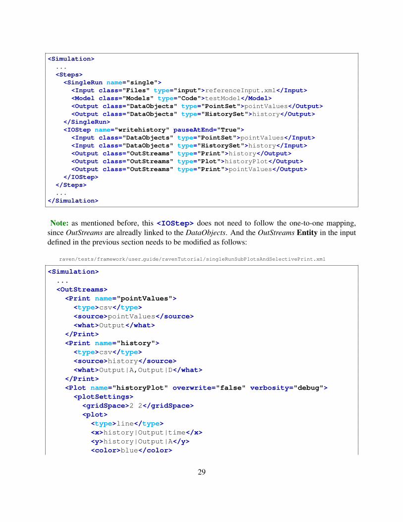
2.3.2 Sub-plot and selectively printing.
This section shows how to use RAVEN to create sub-plots (multiple plots in the same figure) andhow to select only some variable from the DataObjects in the Print OutStream.The goals of this Section are about learning how to:
1. Print out what contained in the DataObjects, selecting only few variables
2. Generate sub-plots (multiple plots in the same figure) of the code results
To accomplish these tasks, the <IOStep> needs to be modified as follows:
raven/tests/framework/user guide/ravenTutorial/singleRunSubPlotsAndSelectivePrint.xml
28
<Simulation>...<Steps>
<SingleRun name="single"><Input class="Files" type="input">referenceInput.xml</Input><Model class="Models" type="Code">testModel</Model><Output class="DataObjects" type="PointSet">pointValues</Output><Output class="DataObjects" type="HistorySet">history</Output>
</SingleRun><IOStep name="writehistory" pauseAtEnd="True"><Input class="DataObjects" type="PointSet">pointValues</Input><Input class="DataObjects" type="HistorySet">history</Input><Output class="OutStreams" type="Print">history</Output><Output class="OutStreams" type="Plot">historyPlot</Output><Output class="OutStreams" type="Print">pointValues</Output>
</IOStep></Steps>...
</Simulation>
Note: as mentioned before, this <IOStep> does not need to follow the one-to-one mapping,since OutStreams are alreadly linked to the DataObjects. And the OutStreams Entity in the inputdefined in the previous section needs to be modified as follows:
raven/tests/framework/user guide/ravenTutorial/singleRunSubPlotsAndSelectivePrint.xml
<Simulation>...<OutStreams><Print name="pointValues">
<type>csv</type><source>pointValues</source><what>Output</what>
</Print><Print name="history">
<type>csv</type><source>history</source><what>Output|A,Output|D</what>
</Print><Plot name="historyPlot" overwrite="false" verbosity="debug">
<plotSettings><gridSpace>2 2</gridSpace><plot>
<type>line</type><x>history|Output|time</x><y>history|Output|A</y><color>blue</color>
29
<gridLocation><x>0</x><y>0</y>
</gridLocation></plot><plot>
<type>line</type><x>history|Output|time</x><y>history|Output|B</y><color>red</color><gridLocation>
<x>1</x><y>0</y>
</gridLocation></plot><plot>
<type>line</type><x>history|Output|time</x><y>history|Output|C</y><color>yellow</color><gridLocation>
<x>0</x><y>1</y>
</gridLocation></plot><plot>
<type>line</type><x>history|Output|time</x><y>history|Output|D</y><color>black</color><gridLocation>
<x>1</x><y>1</y>
</gridLocation></plot><xlabel>time (s)</xlabel><ylabel>evolution (kg)</ylabel>
</plotSettings><actions><how>png</how><title>
<text> </text></title>
</actions></Plot>
30
</OutStreams>...
</Simulation>
1. Print: With respect to the Print nodes defined in the previous section, it can be noticed thatan additional node has been added: <what>. The Print Entity “pointValues” is going toextract and dump only the variables that are part of the Output space (A,B,C,D and notInputP laceHolder). The Print Entity “history” is instead going to print the Output spacevariables A and D.
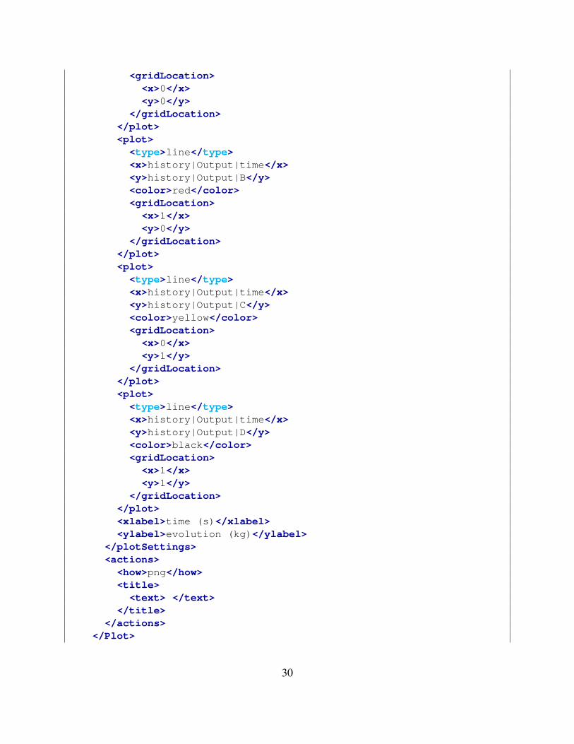
2. Plot: Note that the Plot Entity does not differ much with respect to the one in previoussection: 1) the additional sub-node <gridSpace> has been added. This node is needed todefine how the figure needs to be partitioned (discretization of the grid). In this case a 2 by2 grid is requested. 2) in each <plot> the node <gridLocation> is placed in order tospecify in which position the relative plot needs to be placed. For example, in the followinggrid location, the relative plot is going to be placed at the bottom-right corner.
<gridLocation><x>1</x><y>1</y>
</gridLocation>
The printed data will dump to the CSV file history 0.csv, and Figure 6 reports the four plots(four variables) drawn in the same picture.
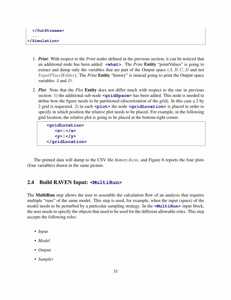
2.4 Build RAVEN Input: <MultiRun>
The MultiRun step allows the user to assemble the calculation flow of an analysis that requiresmultiple “runs” of the same model. This step is used, for example, when the input (space) of themodel needs to be perturbed by a particular sampling strategy. In the <MultiRun> input block,the user needs to specify the objects that need to be used for the different allowable roles. This stepaccepts the following roles:
• Input
• Model
• Output
• Sampler
31

Figure 6. Subplot of the history for variables A,B,C,D.
• Optimizer
• SolutionExport
MultiRun is intended to handle calculations that involve multiple runs of a driven code (sam-pling strategies). Firstly, the RAVEN input file associates the variables to a set of PDFs and to asampling strategy. The “multi-run” step is used to perform several runs in a block of a model (e.g.in a MC sampling).
As shown in Figure 7, at the beginning of each sub sequential run, the sampler provides the newvalues of the variables to be perturbed. The code API places those values in the input file. At thispoint, the code API generates the run command and asks to be queued by the job handler. The jobhandler manages the parallel execution of as many runs as possible within a user prescribed rangeand communicates with the step controller when a new set of output files are ready to be processed.The code API receives the new input files and collects the data in the RAVEN internal format. Thesampler is queried to assess if the sequence of runs is ended, if not, the step controller asks fora new set of values from the sampler and the sequence is restarted. The job handler is currently
32
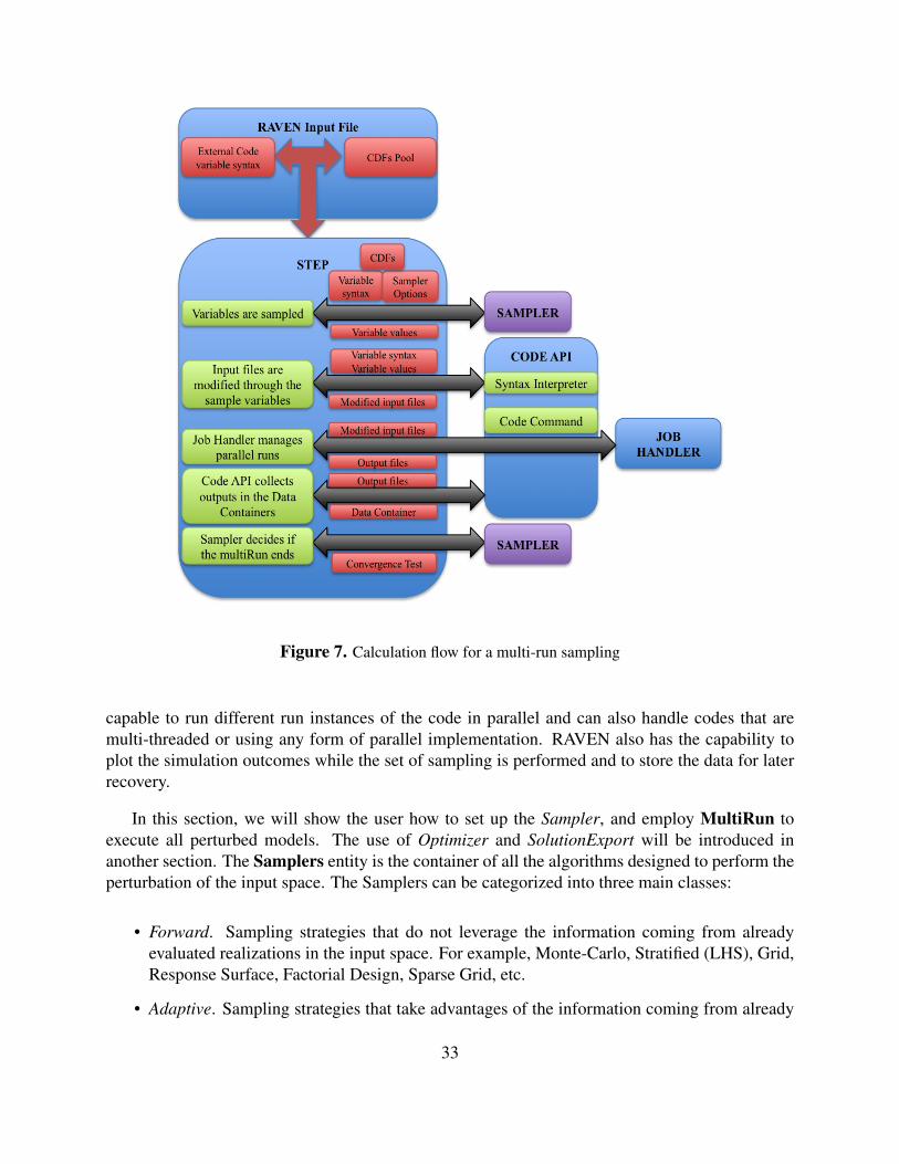
Figure 7. Calculation flow for a multi-run sampling
capable to run different run instances of the code in parallel and can also handle codes that aremulti-threaded or using any form of parallel implementation. RAVEN also has the capability toplot the simulation outcomes while the set of sampling is performed and to store the data for laterrecovery.
In this section, we will show the user how to set up the Sampler, and employ MultiRun toexecute all perturbed models. The use of Optimizer and SolutionExport will be introduced inanother section. The Samplers entity is the container of all the algorithms designed to perform theperturbation of the input space. The Samplers can be categorized into three main classes:
• Forward. Sampling strategies that do not leverage the information coming from alreadyevaluated realizations in the input space. For example, Monte-Carlo, Stratified (LHS), Grid,Response Surface, Factorial Design, Sparse Grid, etc.
• Adaptive. Sampling strategies that take advantages of the information coming from already
33
evaluated realizations of the input space, adapting the sampling strategies to key figures ofmerits. For example, Limit Surface search, Adaptive sparse grid, etc.
• Dynamic Event Tree. Sampling strategies that perform the exploration of the input spacebased on the dynamic evolution of the system, employing branching techniques. For exam-ple, Dynamic Event Tree, Hybrid Dynamic Event Tree, etc.
The sampler is probably the most important entity in the RAVEN framework. It provides manydifferent sampling strategies that can be used in almost all RAVEN related applications. In thissection, we will only illustrate the simplest forward sampler, i.e. Monte-Carlo, to familarize theuser with the use of sampler. Monte-Carlo method is one of the most-used methodologies in severalmathematic disciplines. The theory of this method can be found in the RAVEN theory manual. Inaddition, we will continue to use the AnalyticBateman to illustrate the setup of MultiRun andSamplers. In order to accomplish these tasks, the following precedures or RAVEN entities areneeded:
1. Set up the running environment: <RunInfo>
2. Provide the required files: <Files>
3. Link between RAVEN and dirven code: <Models>
4. Define probability distribution functions for inputs: <Distributions>
5. Set up a simple Monte-Carlo sampling for perturbing the input space: <Samplers>
6. Store the input and output data: <DataObjects>
7. Print and plot input and output data: <OutStreams>
8. Control multiple executions: <Steps>
In section 2.2, we have already discussed the use of <RunInfo>, <Files>, <Models>,<DataObjects>, <OutStreams>. For practice, the user can try to build these RAVEN enti-ties by themselves, and refer to the complete input file located at raven/tests/framework/user guide/ravenTutorial/MonteCarlo.xml. In this section, we’d like to show the users how to set up <Distributions>,<Samplers> and MultiRun of <Steps>. RAVEN employs <Distributions> to definemany different probability distribution functions (PDFs) that can be used to characterize the in-put parameters. One can consider the <Distributions> entity to be a container of all thestochastic representation of random variables. Currently, RAVEN supports:
• 1-Dimensional continuous and discrete distributions, such as Normal, Weibull, Binomial,etc.
34

• N-Dimensional distributions, such as Multivariate Normal, user-inputted N-Dimensional dis-tributions.
For the AnalyticBateman example, two 1-D uniform distributions are defined:
• sigma ∼ U(1, 10), used to model the uncertainties associated with the sigma Model vari-ables;
• decayConstant ∼ U(0.5e− 8, 1e− 8), used to model the uncertainties associated with theModel variable decay constants. Note that the same distribution can be re-used for multipleinput variables, while still keeping those variables independent.
The following is the definition of <Distributions> block that is used for the AnalyticBate-man problem:
raven/tests/framework/user guide/ravenTutorial/MonteCarlo.xml
<Simulation>...<Distributions>
<Uniform name="sigma"><lowerBound>1</lowerBound><upperBound>10</upperBound>
</Uniform><Uniform name="decayConstant">
<lowerBound>0.000000005</lowerBound><upperBound>0.000000010</upperBound>
</Uniform></Distributions>...
</Simulation>
For uniform distributions, only <lowerBound> and <upperBound> are required. For otherdistributions, please refer to the RAVEN user manual.
As we already mentioned, we will employ Monte-Carlo sampling strategy to demonstrate Mul-tiRun. To employ the Monte-Carlo sampling strategy, a <MonteCarlo> node needs to be de-fined. The user also needs to specify the variables that need to be sampled using <variable>.In addition, the setting for this sampler need to be specified in the <samplerInit> block. Theonly required sub-node <limit> is used to specify the number of Monte Carlo samples. Theuser can also use other optional sub-node to characterize their samplers. For this example, the<Samplers> block is:
raven/tests/framework/user guide/ravenTutorial/MonteCarlo.xml
35
<Simulation>...<Samplers>
<MonteCarlo name="monteCarlo"><samplerInit><limit>100</limit><reseedEachIteration>True</reseedEachIteration><initialSeed>0</initialSeed>
</samplerInit><variable name="sigma-A"><distribution>sigma</distribution>
</variable><variable name="decay-A"><distribution>decayConstant</distribution>
</variable></MonteCarlo>
</Samplers>...
</Simulation>
In this case, the Monte-Carlo method is employed on two model variables, each of which arelisted by name and are associated with a distribution. Note that the decay- and sigma- variablesare associated with the distributions decayConstant and sigma, respectively. These variables andtheir values are passed to the model via the generic code interface. This requires the users to makesome changes in their input files in order to accept these variables. For example, the input file ofAnalyticBateman becomes:
raven/tests/framework/user guide/ravenTutorial/commonFiles/referenceInput generic CI.xml
<AnalyticalBateman>...<nuclides>
<A><equationType>N1</equationType><initialMass>1.0</initialMass><decayConstant>$RAVEN-decay-A|10$</decayConstant><sigma>$RAVEN-sigma-A|10$</sigma><ANumber>230</ANumber>
</A><B>
<equationType>N2</equationType><initialMass>1.0</initialMass>
36
<decayConstant>0.000000007</decayConstant><sigma>5</sigma><ANumber>200</ANumber>
</B><C>
<equationType>N3</equationType><initialMass>1.0</initialMass><decayConstant>0.000000008</decayConstant><sigma>3</sigma><ANumber>150</ANumber>
</C><D>
<equationType>N4</equationType><initialMass>1.0</initialMass><decayConstant>0.000000009</decayConstant><sigma>1</sigma><ANumber>100</ANumber>
</D></nuclides>...
</AnalyticalBateman>
As shown in this example, the values of nodes <sigma> and <decayConstant> are re-placed with variables ’$RAVEN-decay-A|10$’ and ’$RAVEN-sigma-A|10$’, respec-tively. Note: we use prefix ’RAVEN-’ + ’variable names defined inside RAVENinput files’ within ’$ $’ to define the RAVEN-editable input parameters. In other words,the RAVEN-editable input parameters is used to transfer the sampled values of RAVEN variablesto input parameters of given code. This is the only way to connect the input parameters of codewith variables of RAVEN if Generic code interface is employed. In addition, we use the wild-cards| to define the format of the value of the RAVEN-editable input parameters. In this case, the valuethat is going to be replaced by the generic code interface will be left-justified with a string lengthof 10 (e.g. “|10”). Other formatting options can be found in the RAVEN user manual.
As we already mentioned, the Generic code interface requires that the codes need to return aCSV file with the input parameters and output parameters. The filename of the CSV file shouldincludes:
• prefix: “out∼”
• filename: the base of input filename without extension
• extension: “.csv”
37

For this case, the input filename is “referenceInput generic CI.xml”, thus the output CSV filenameshould be “out∼referenceInput generic CI.csv”.
Once all the other entities are defined in the RAVEN input file, they must be combined inthe <Steps> block, which dictates the workflow of RAVEN. For this case, two <Steps> aredefined:
• <MultiRun> “sample”, used to run the multiple instances of the driven code and collectthe outputs in the two DataObjects. As it can be seen, the <Sampler> is specified tocommunicate to the Step that the driven code needs to be perturbed through the Monte-Carlosampling.
• <IOStep> named “writeHistories”, used to 1) dump the “histories” and “samples” DataOb-jects Entity to a CSV file and 2) plot the data in the EPS file.
Figures 8 and 9 show the report generated by RAVEN of the evolution of the variable A andits final values, respectively.
raven/tests/framework/user guide/ravenTutorial/MonteCarlo.xml
<Simulation>...<Steps>
<MultiRun name="sample"><Input class="Files" type="input">referenceInput.xml</Input><Model class="Models" type="Code">testModel</Model><Sampler class="Samplers" type="MonteCarlo">monteCarlo</Sampler><Output class="DataObjects" type="PointSet">samples</Output><Output class="DataObjects" type="HistorySet">histories</Output>
</MultiRun><IOStep name="writeHistories" pauseAtEnd="True"><Input class="DataObjects" type="HistorySet">histories</Input><Input class="DataObjects" type="PointSet">samples</Input><Output class="OutStreams" type="Plot">samplesPlot_A</Output><Output class="OutStreams" type="Plot">history_A</Output><Output class="OutStreams" type="Print">histories</Output>
</IOStep></Steps>...
</Simulation>
38
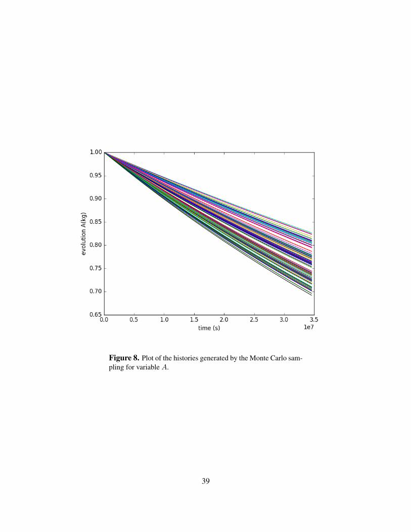
Figure 8. Plot of the histories generated by the Monte Carlo sam-pling for variable A.
39

Figure 9. Plot of the samples generated by the MC sampling forvariable A.
40
2.5 Build RAVEN Input: <RomTrainer>
The RomTrainer step type performs the training of a Reduced Order Model (ROM), and thespecifications of this step must be defined within a <RomTrainer> block. ROMs, also known asa surrogate model, are used to lower the computational cost, reducing the number of needed pointsand prioritizing the area of the input space that needs to be explored when the simulations usingthe high-fidelity codes are very expensive. ROMs can be considered as an artificial representationof the link between the input and output spaces for a particular system.
In most of the cases of interest, the information that is sought is related to defining the failureboundaries of a system with respect to perturbations in the input space. For this reason, in thedevelopment of RAVEN, it has been given priority to the introduction of a class of supervisedlearning algorithms, which are usually referred to as classifiers. A classifier is a reduced ordermodel that is capable of representing the system behavior through a binary response (failure/suc-cess). Currently, RAVEN supports around 40 different ROM methodologies. All these supervisedlearning algorithms have been imported via an API from the Scikit-Learn library. In addition, theN-Dimensional spline and the inverse weight methods that are currently available for the interpo-lation of N-Dimensional PDF/CDF, can also be used as ROMs.
In this section, the N-dimensional inverse weight method is employed to construct ROM tofamilarize the user with the use of ROMs. Inverse distance weighting (IDW) is a type of deter-ministic method for multivariate interpolation with a known scattered set of points. The assignedvalues to unknown points are calculated via a weighted average of the values available at the knownpoints.It is important to NOTE that RAVEN uses a Z-score normalization of the training data beforeconstructing the NDinvDistWeight ROM:
X′ =(X− µ)
σ(3)
2.5.1 How to train and output a ROM?
In general, the “training” is a process that use sampling of the physical model to improve the pre-diction capability of the ROM. As mentioned before, RAVEN provides lots of different samplingstrategies, such as Monte Carlo, Grid, Stratified (e.g. LHS), and Stochastic Collocation methods.All of them can be used to train a ROM. In this section, we will continue to use AnalyticBatemanto illustrate the setup of RomTrainer. As before, a simple step MultiRun with Monte Carlosampler is employed to generate the data set that can be used to train the ROM. The full RAVENinput file can be found: raven/tests/framework/user guide/ravenTutorial/RomTrain.xml. Becausethe setup of MultiRun is the same as previous example in section 2.4, the RAVEN input file aboutthe MultiRun is not include in this section. However, the full precedures are listed here to make
41
the user better understand the construction of ROM. The following precedures or RAVEN entitiesare needed:
• MultiRun: Monte Carlo sampling to generate the data set
1. Set up the running environment: <RunInfo>;
2. Provide the required files: <Files>;
3. Link between RAVEN and dirven code: <Code>;
4. Define probability distribution functions for inputs: <Distributions>;
5. Set up a simple Monte-Carlo sampling for perturbing the input space: <Samplers>;
6. Store the input and output data: <DataObjects>;
7. Print and plot input and output data: <OutStreams>;
8. Control multiple executions: <MultiRun>.
• RomTrainer: Train the ROM with given data set
1. Specify the type of ROMs: <ROM>;
2. Provide the data set for ROM training: <DataObjects>;
3. Train the ROM: <RomTrainer>;
4. Dump the ROM: <IOStep>
The specifications of the reduced order model must be defined within <ROM>XML block. ThisXML node accepts the following attributes:
• name, required string attribute, user-defined identifier of this model.
• subType, required string attribute, defines which of the sub-types should be used, choos-ing among the previously reported types.
In the <ROM> input block, the following XML sub-nodes are required, independent of thesubType specified:
• <Features>, comma separated string, required field, specifies the names of the featuresof this ROM. Note: These parameters are going to be requested for the training of thisobject;
• <Target>, comma separated string, required field, contains a comma separated list ofthe targets of this ROM. These parameters are the Figures of Merit (FOMs) this ROM issupposed to predict. Note: These parameters are going to be requested for the training ofthis object.
42
For each sub-type specified in the attribute subType, additional sub-nodes may be required(Please check the RAVEN user manual for each ROM). In addition, if an <HistorySet> isprovided in the training step, then a temporal ROM is created, i.e. a ROM that generates not asingle value prediction of each element indicated in the <Target> block but its full temporalprofile. In this section, a time-dependent ROM will be constructed.
In order to use N-dimensional inverse distance weighting ROM, the <ROM> attribute subTypeneeds to be ’NDinvDistWeight’. The following addition sub-node is also required.
• <p>, integer, required field, must be greater than zero and represents the “power param-eter”. For the choice of value for <p>,it is necessary to consider the degree of smoothingdesired in the interpolation/extrapolation, the density and distribution of samples being inter-polated, and the maximum distance over which an individual sample is allowed to influencethe surrounding ones (lower p means greater importance for points far away).
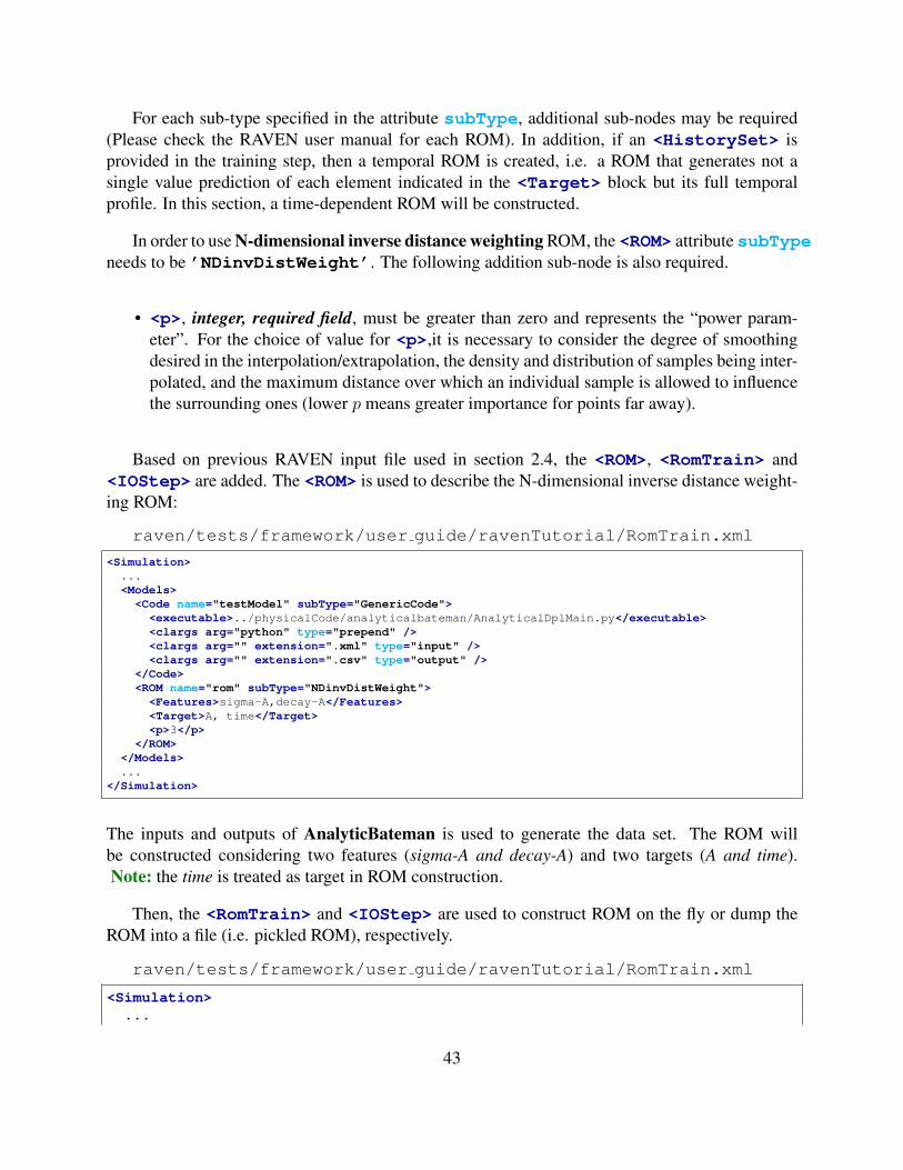
Based on previous RAVEN input file used in section 2.4, the <ROM>, <RomTrain> and<IOStep> are added. The <ROM> is used to describe the N-dimensional inverse distance weight-ing ROM:
raven/tests/framework/user guide/ravenTutorial/RomTrain.xml
<Simulation>...<Models><Code name="testModel" subType="GenericCode">
<executable>../physicalCode/analyticalbateman/AnalyticalDplMain.py</executable><clargs arg="python" type="prepend" /><clargs arg="" extension=".xml" type="input" /><clargs arg="" extension=".csv" type="output" />
</Code><ROM name="rom" subType="NDinvDistWeight">
<Features>sigma-A,decay-A</Features><Target>A, time</Target><p>3</p>
</ROM></Models>...
</Simulation>
The inputs and outputs of AnalyticBateman is used to generate the data set. The ROM willbe constructed considering two features (sigma-A and decay-A) and two targets (A and time).Note: the time is treated as target in ROM construction.
Then, the <RomTrain> and <IOStep> are used to construct ROM on the fly or dump theROM into a file (i.e. pickled ROM), respectively.
raven/tests/framework/user guide/ravenTutorial/RomTrain.xml
<Simulation>...
43

<Steps><MultiRun name="sample"><Input class="Files" type="input">referenceInput.xml</Input><Model class="Models" type="Code">testModel</Model><Sampler class="Samplers" type="MonteCarlo">monteCarlo</Sampler><Output class="DataObjects" type="HistorySet">histories</Output>
</MultiRun><RomTrainer name="trainROM"><Input class="DataObjects" type="HistorySet">histories</Input><Output class="Models" type="ROM">rom</Output>
</RomTrainer><IOStep name="dumpROM"><Input class="Models" type="ROM">rom</Input><Output class="Files" type="">rom_inv</Output>
</IOStep><IOStep name="writeHistories" pauseAtEnd="True"><Input class="DataObjects" type="HistorySet">histories</Input><Output class="OutStreams" type="Print">histories</Output>
</IOStep></Steps>...
</Simulation>
The ’HistorySet’ generated by the “sample” step is used as input of the “trainROM” step.The output of the “trainROM” is “rom” which is predefined in <ROM>. If a ’PointSet’ isprovided as input, the output “rom” will be time-independent. The “dumpROM” step is used toserialize the “rom” to file (pickled). In this example, the file is identified in <Files>.
raven/tests/framework/user guide/ravenTutorial/RomTrain.xml
<Simulation>...<Files>
<Input name="referenceInput.xml" type="input">../commonFiles/referenceInput_generic_CI.xml
</Input><Input name="rom_inv" type="">inverseRom.pk</Input>
</Files>...
</Simulation>
A pickled file with name “inverseRom.pk” will be generated in the working directory. This pickledROM can be reused by RAVEN to perform additional analysis, and we will introduce this capabil-ity in the following section. Since we have four different steps to execute, the <RunInfo> blockis modified:
raven/tests/framework/user guide/ravenTutorial/RomTrain.xml
44

<Simulation>...<RunInfo><JobName>RomTrain</JobName><Sequence>sample, trainROM, dumpROM, writeHistories</Sequence><WorkingDir>ROM</WorkingDir><batchSize>1</batchSize>
</RunInfo>...
</Simulation>
The <Sequence> is used to provide an ordered list of the step names that RAVEN will run.
2.5.2 How to load and sample a ROM?
In previous section, we have shown that RAVEN can be used to train a ROM and output the ROMto a pickled file. In this section, we will show the user how to load the pickled ROM, and how toreuse it inside RAVEN environment. In general, a <ROM> with subtype ’pickledROM’ is usedto hold the place of the ROM that will be loaded from file. The notation for this ROM is much lessthan a typical ROM; it only requires a name and its subtype.
Example: For this example the ROM has already been created and trained in another RAVENrun, then pickled to a file called rom pickle.pk. In the example, the file is identified in<Files>, the model is defined in <Models>, and the model loaded in <Steps>.
<Simulation>...<Files>
<Input name="rompk" type="">rom_pickle.pk</Input></Files>...<Models>
...<ROM name="myRom" subType="pickledROM"/>...
</Models>...<Steps>
...<IOStep name="loadROM"><Input class="Files" type="">rompk</Input><Output class="Models" type="ROM">myRom</Output>
</IOStep>...
</Steps>...
45

</Simulation>
Note: When loading ROMs from file, RAVEN will not perform any checks on the expectedinputs or outputs of a ROM; it is expected that a user knows at least the I/O of a ROM before tryingto use it as a model. However, RAVEN does require that pickled ROMs be trained before picklingin the first place.
Initially, a pickled ROM is not usable. It can not be trained or sampled; attempting to doso will raise an error. An <IOStep> is used to load the ROM from file, at which point theROM will have all the same characteristics as when it was pickled in a previous RAVEN run.Take AnalyticBateman for example, the pickled ROM “inverseRom.pk” is generated in previoussection and copied to the commonFiles folder, RAVEN use the Files object to track the pickledROM file.
raven/tests/framework/user guide/ravenTutorial/RomLoad.xml
<Simulation>...<Files>
<Input name="rom_inv" type="">../commonFiles/inverseRom.pk</Input></Files>...
</Simulation>
In this example, the subtype ’NDinvDistWeight’ of <ROM> is used instead of ’pickledROM’,since the subtype of ROM is already known.
raven/tests/framework/user guide/ravenTutorial/RomLoad.xml
<Simulation>...<Models>
<ROM name="rom" subType="NDinvDistWeight"><Features>sigma-A,decay-A</Features><Target>A, time</Target><p>3</p>
</ROM></Models>...
</Simulation>
Two data objects are defined: 1) a HistorySet named “inputPlaceHolder” used as a place-holder input for the ROM sampling step, 2) a HistorySet named “histories” used to store the ROMresponses from Monte Carlo samples.
46

raven/tests/framework/user guide/ravenTutorial/RomLoad.xml
<Simulation>...<DataObjects>
<PointSet name="inputPlaceHolder"><Input>sigma-A,decay-A</Input><Output>OutputPlaceHolder</Output>
</PointSet><HistorySet name="histories">
<Input>sigma-A,decay-A</Input><Output>A, time</Output><options><pivotParameter>time</pivotParameter>
</options></HistorySet>
</DataObjects>...
</Simulation>
Note: In this example, a time-dependent ROM trained in previous case is used here. ’time’is identified as Output. The sub-node <pivotParameter> can be used to define the pivotvariable (e.g. time) that is non-decreasing in the input HistorySet.
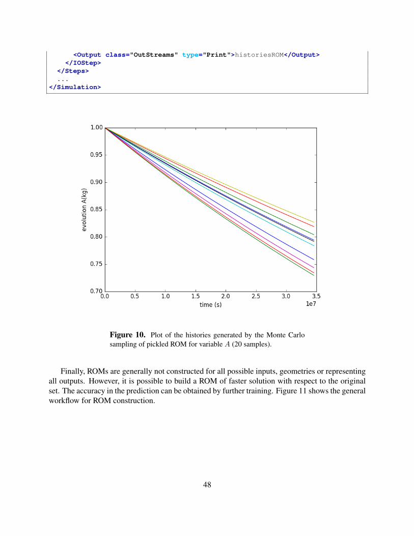
As mentioned before, the <IOStep> is used to load the pickled ROM. In addition, the <MultiRun>is used to sample the ROM using Monte Carlo method. Another <IOStep> is used to output theresponses of ROM into a CSV file. Figure 10 shows the different evolutions of the variable A forall 20 samples.
raven/tests/framework/user guide/ravenTutorial/RomLoad.xml
<Simulation>...<Steps>
<IOStep name="loadROM"><Input class="Files" type="">rom_inv</Input><Output class="Models" type="ROM">rom</Output>
</IOStep><MultiRun name="sampleROM"><Input class="DataObjects" type="PointSet">inputPlaceHolder</Input><Model class="Models" type="ROM">rom</Model><Sampler class="Samplers" type="MonteCarlo">monteCarlo</Sampler><Output class="DataObjects" type="HistorySet">histories</Output>
</MultiRun><IOStep name="writeHistories" pauseAtEnd="True"><Input class="DataObjects" type="HistorySet">histories</Input><Output class="OutStreams" type="Plot">historyROMPlot</Output>
47
<Output class="OutStreams" type="Print">historiesROM</Output></IOStep>
</Steps>...
</Simulation>
Figure 10. Plot of the histories generated by the Monte Carlosampling of pickled ROM for variable A (20 samples).
Finally, ROMs are generally not constructed for all possible inputs, geometries or representingall outputs. However, it is possible to build a ROM of faster solution with respect to the originalset. The accuracy in the prediction can be obtained by further training. Figure 11 shows the generalworkflow for ROM construction.
48
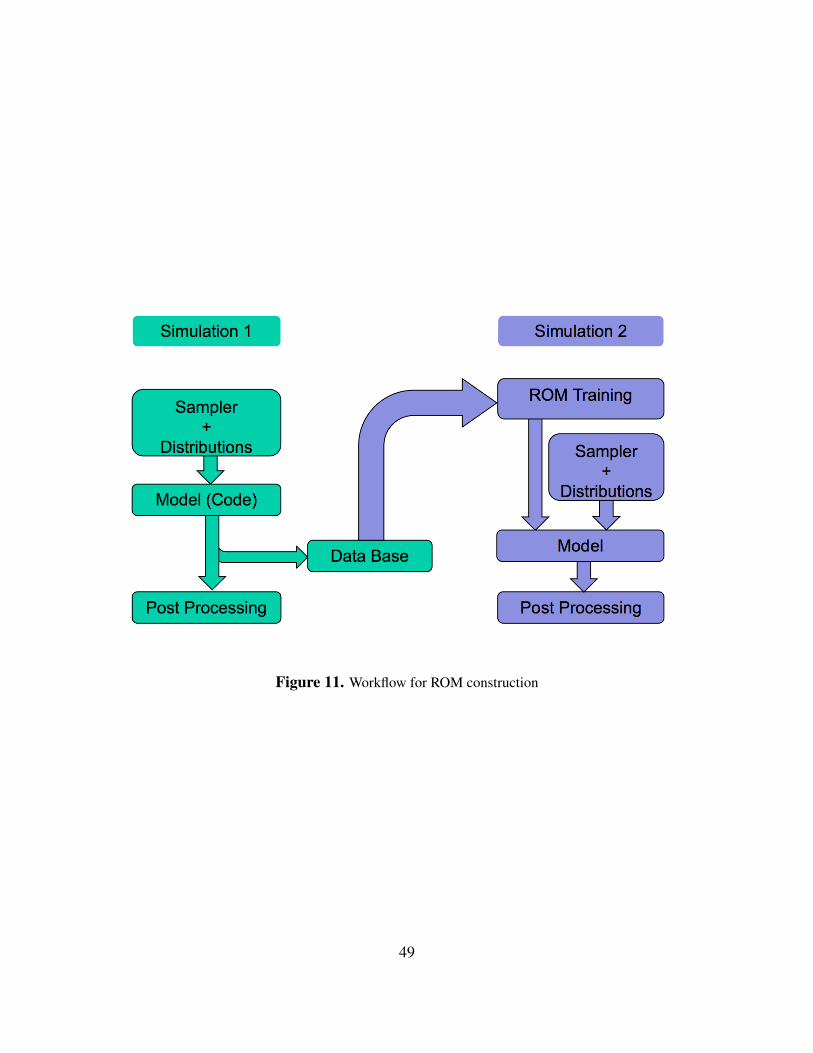
Figure 11. Workflow for ROM construction
49
2.6 Build RAVEN Input: <PostProcess>
The PostProcess step is used to post-process data or manipulate RAVEN entities. It is intendedto perform a single action that is employed by a Model of type PostProcessor. The specificationof this type of step is defined within a <PostProcess> XML block. As for the other objects,the attribute name is required and is used to refer to this specific entity in the <RunInfo> blockunder the <Sequence> node.
In the <PostProcess> input block, the user needs to specify the objects needed for thedifferent allowable roles. This step requires the following roles:
• <Input>: accepts Files, DataObjects or Databases.
• <Model>: Only ’Models’ and ’PostProcessor’ can be assigned to the node’s at-tributes class and type, respectively.
• <Output>: accepts Files, DataObjects, Databases or OutStreams.
As mentioned before, only the model with type PostProcessor is allowed for this step. A post-processor can be considered as an action performed on a set of data or other type of objects. Mostof the post-processors contained in RAVEN, employ a mathematical operation on the data givenas “Input”. Currently, the following PostProcessor are available in RAVEN:
• BasicStatistics• ComparisonStatistics• ImportanceRank• SafestPoint• LimitSurface• LimitSurfaceIntegral• External• TopologicalDecomposition• RavenOutput• DataMining
One can use the node attribute subType to select which of the post-processors to be used. Aswith other objects, the attribute name is always required so that other RAVEN input XML blockscan use this name to refer to this specific entity. In addition, each post-processor may require extrasub-nodes, and the user can refer to the RAVEN user manual for the detailed specifications.
50
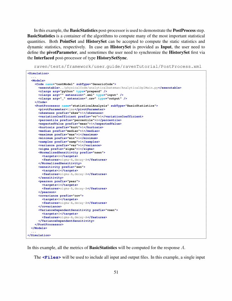
In this example, the BasicStatistics post-processor is used to demonstrate the PostProcess step.BasicStatistics is a container of the algorithms to compute many of the most important statisticalquantities. Both PointSet and HistorySet can be accepted to compute the static statistics anddynamic statistics, respectively. In case an HistorySet is provided as Input, the user need todefine the pivotParameter, and sometimes the user need to synchronize the HistorySet first viathe Interfaced post-processor of type HistorySetSync.
raven/tests/framework/user guide/ravenTutorial/PostProcess.xml
<Simulation>...<Models><Code name="testModel" subType="GenericCode">
<executable>../physicalCode/analyticalbateman/AnalyticalDplMain.py</executable><clargs arg="python" type="prepend" /><clargs arg="" extension=".xml" type="input" /><clargs arg=" " extension=".csv" type="output" />
</Code><PostProcessor name="statisticalAnalysis" subType="BasicStatistics">
<pivotParameter>time</pivotParameter><skewness prefix="skew">A</skewness><variationCoefficient prefix="vc">A</variationCoefficient><percentile prefix="percentile">A</percentile><expectedValue prefix="mean">A</expectedValue><kurtosis prefix="kurt">A</kurtosis><median prefix="median">A</median><maximum prefix="max">A</maximum><minimum prefix="min">A</minimum><samples prefix="samp">A</samples><variance prefix="var">A</variance><sigma prefix="sigma">A</sigma><NormalizedSensitivity prefix="nsen">
<targets>A</targets><features>sigma-A,decay-A</features>
</NormalizedSensitivity><sensitivity prefix="sen">
<targets>A</targets><features>sigma-A,decay-A</features>
</sensitivity><pearson prefix="pear">
<targets>A</targets><features>sigma-A,decay-A</features>
</pearson><covariance prefix="cov">
<targets>A</targets><features>sigma-A,decay-A</features>
</covariance><VarianceDependentSensitivity prefix="vsen">
<targets>A</targets><features>sigma-A,decay-A</features>
</VarianceDependentSensitivity></PostProcessor>
</Models>...
</Simulation>
In this example, all the metrics of BasicStatistics will be computed for the response A.
The <Files> will be used to include all input and output files. In this example, a single input
51

file for the driven code and two output files of the PostProcess step are defined here. As shownin the following, two output files are defined for this case study to store the static statistics anddynamic statistics information. The ’time’ is used as the <pivotParameter>.
raven/tests/framework/user guide/ravenTutorial/PostProcess.xml
<Simulation>...<Files>
<Input name="referenceInput.xml" type="input">../commonFiles/referenceInput_generic_CI.xml
</Input><Input name="output_1" type="">static.xml</Input><Input name="output_2" type="">time.xml</Input>
</Files>...
</Simulation>
As before, all defined RAVEN entities are combined in the <Steps> block.
raven/tests/framework/user guide/ravenTutorial/PostProcess.xml<Simulation>...<Steps>
<MultiRun name="sampleMC"><Input class="Files" type="input">referenceInput.xml</Input><Model class="Models" type="Code">testModel</Model><Sampler class="Samplers" type="MonteCarlo">mc</Sampler><Output class="DataObjects" type="PointSet">samplesMC</Output><Output class="DataObjects" type="HistorySet">histories</Output>
</MultiRun><PostProcess name="statAnalysis_1">
<Input class="DataObjects" type="PointSet">samplesMC</Input><Model class="Models" type="PostProcessor">statisticalAnalysis</Model><Output class="DataObjects" type="PointSet">statisticalAnalysis_basicStatPP</Output><Output class="OutStreams" type="Print">statisticalAnalysis_basicStatPP_dump</Output>
</PostProcess><PostProcess name="statAnalysis_2">
<Input class="DataObjects" type="HistorySet">histories</Input><Model class="Models" type="PostProcessor">statisticalAnalysis</Model><Output class="DataObjects" type="HistorySet">statisticalAnalysis_basicStatPP_time</Output><Output class="OutStreams" type="Print">statisticalAnalysis_basicStatPP_time_dump</Output>
</PostProcess></Steps>...
</Simulation>
In this case, three steps have been defined:
• <MultiRun> named “sampleMC”, used to run the multiple instances of the driven codeand collect the outputs in the two DataObjects. As it can be seen, the <Sampler> isinputted to communicate to the Step that the driven code needs to be perturbed through theMonte Carlo sampling strategy.
• <PostProcess> named “statAnalysis 1”, is used to compute all the statistical momentsand FOMs based on the data obtained through the sampling strategy. As it can be noticed,
52

the ’PointSet’ “samplesMC” is used as input to compute the static statistics.
• <PostProcess> named “statAnalysis 2”, is used to compute all the statistical momentsand FOMs based on the data obtained through the sampling strategy. As it can be noticed,the ’HistorySet’ “histories” is used as input to compute the dynamic statistics.
53
3 Forward Sampling Strategies
In order to perform UQ and dynamic probabilistic risk assessment (DPRA), a sampling strategyneeds to be employed. The sampling strategy perturbs the input space (domain of the uncertainties)to explore the response of a complex system in relation to selected FOMs.
The most widely used strategies to perform UQ and PRA are generally collected in RAVEN asForward samplers. Forward samplers include all the strategies that simply perform the samplingof the input space. These strategies sample without exploiting, through learning approaches, theinformation made available from the outcomes of evaluation previously performed (adaptive sam-pling) and the common system evolution (patterns) that different sampled calculations can generatein the phase space (Dynamic Event Tree).
As mentioned in Section ??, RAVEN has several different Forward samplers:
• Monte-Carlo
• Grid-based
• Stratified and its specialization named Latin Hyper Cube.
In addition, RAVEN posses advanced Forward sampling strategies that:
• Build a grid in the input space selecting evaluation points based on characteristic quadraturesas part of stochastic collocation for generalized polynomial chaos method (Sparse Grid Col-location sampler);
• Use high-density model reduction (HDMR) a.k.a. Sobol decomposition to approximate afunction as the sum of interactions with increasing complexity (Sobol sampler).
In the following subsections, we provide examples of input files in RAVEN using the method, withexplanatory commentary.
3.1 Monte-Carlo sampling through RAVEN
The Monte-Carlo method is one of the most-used methodologies in several mathematic disciplines.In this section, we will explain the techniques for employing this methodology in RAVEN, and werecommend the user to read the theory manual to explore the theory of the method. The goals ofthis section are about learning how to:
1. Set up a simple Monte-Carlo sampling for perturbing the input space of a driven code
54

2. Load the outputs of the code into RAVEN DataObjects (HistorySets and PointSets)
3. Print the contents of DataObjects to file
4. Generate plots of the sampling results.
In order to accomplish these tasks, the following RAVEN Entities (XML blocks in the RAVENinput file) are needed:
1. RunInfo:
raven/tests/framework/user guide/ForwardSamplingStrategies/forwardSamplingMontecarlo.xml
<Simulation>...<RunInfo>
<JobName>RunDir/MonteCarlo</JobName><Sequence>sample,writeHistories</Sequence><WorkingDir>RunDir/MonteCarlo</WorkingDir><batchSize>1</batchSize>
</RunInfo>...
</Simulation>
As discussed in Section ??, the RunInfo Entity sets up the analysis that the user wantsto perform. In this specific case, two steps (<Sequence>) are sequentially run using 12processors (<batchSize>). This means that 12 instances of the driven code are run simul-taneously. Every time a simulation ends, a new one is launched. Note that the <JobName>is not required, but is useful in identifying the input file.
2. Files:raven/tests/framework/user guide/ForwardSamplingStrategies/forwardSamplingMontecarlo.xml
<Simulation>...<Files>
<Input name="referenceInput.xml"type="input">referenceInput.xml</Input>
</Files>...
</Simulation>
Since the driven code uses a single input file, in this section the original input is identifiedand named. As detailed in the user manual, the attribute name represents the alias that isused in all the other input blocks in order to refer to this file.
55

3. Models:raven/tests/framework/user guide/ForwardSamplingStrategies/forwardSamplingMontecarlo.xml
<Simulation>...<Models><Code name="testModel" subType="GenericCode">
<executable>../physicalCode/analyticalbateman/AnalyticalDplMain.py</executable><clargs arg="python" type="prepend" /><clargs arg="" extension=".xml" type="input" /><clargs arg=" " extension=".csv" type="output" />
</Code></Models>...
</Simulation>
The Model used in this example is the AnalyticalBateman external model, which is definedin section 2.1. This model uses a keyword-based input file and exports its output file in aCSV format, so the GenericCode interface is used.
4. Distributions:
raven/tests/framework/user guide/ForwardSamplingStrategies/forwardSamplingMontecarlo.xml
<Simulation>...<Distributions>
<Uniform name="sigma"><lowerBound>1</lowerBound><upperBound>10</upperBound>
</Uniform><Uniform name="decayConstant">
<lowerBound>0.000000005</lowerBound><upperBound>0.000000010</upperBound>
</Uniform></Distributions>...
</Simulation>
In the <Distributions> block, the stochastic model for the uncertainties treated by the<Sampler> is defined. In this case two distributions are defined:
• sigma ∼ U(1, 10), used to model the uncertainties associated with the sigma Modelvariables
• decayConstant ∼ U(0.5e−8, 1e−8), used to model the uncertainties associated withthe Model variable decay constants. Note that the same distribution can be re-used formultiple input variables, while still keeping those variables independent.
5. Samplers:
raven/tests/framework/user guide/ForwardSamplingStrategies/forwardSamplingMontecarlo.xml
56
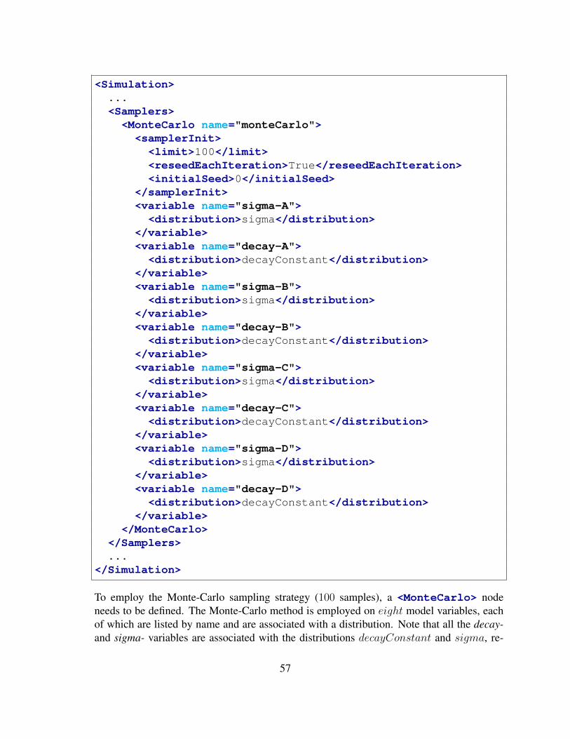
<Simulation>...<Samplers>
<MonteCarlo name="monteCarlo"><samplerInit><limit>100</limit><reseedEachIteration>True</reseedEachIteration><initialSeed>0</initialSeed>
</samplerInit><variable name="sigma-A"><distribution>sigma</distribution>
</variable><variable name="decay-A"><distribution>decayConstant</distribution>
</variable><variable name="sigma-B"><distribution>sigma</distribution>
</variable><variable name="decay-B"><distribution>decayConstant</distribution>
</variable><variable name="sigma-C"><distribution>sigma</distribution>
</variable><variable name="decay-C"><distribution>decayConstant</distribution>
</variable><variable name="sigma-D"><distribution>sigma</distribution>
</variable><variable name="decay-D"><distribution>decayConstant</distribution>
</variable></MonteCarlo>
</Samplers>...
</Simulation>
To employ the Monte-Carlo sampling strategy (100 samples), a <MonteCarlo> nodeneeds to be defined. The Monte-Carlo method is employed on eight model variables, eachof which are listed by name and are associated with a distribution. Note that all the decay-and sigma- variables are associated with the distributions decayConstant and sigma, re-
57
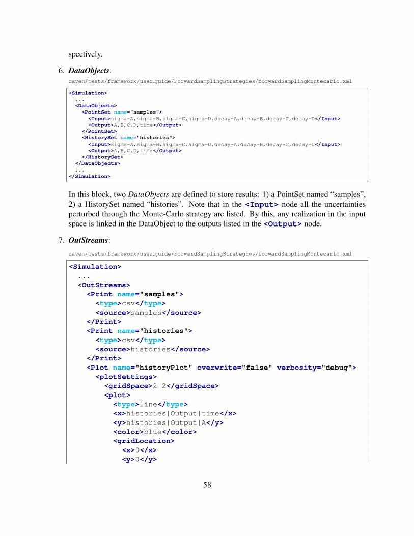
spectively.
6. DataObjects:raven/tests/framework/user guide/ForwardSamplingStrategies/forwardSamplingMontecarlo.xml
<Simulation>...<DataObjects><PointSet name="samples">
<Input>sigma-A,sigma-B,sigma-C,sigma-D,decay-A,decay-B,decay-C,decay-D</Input><Output>A,B,C,D,time</Output>
</PointSet><HistorySet name="histories">
<Input>sigma-A,sigma-B,sigma-C,sigma-D,decay-A,decay-B,decay-C,decay-D</Input><Output>A,B,C,D,time</Output>
</HistorySet></DataObjects>...
</Simulation>
In this block, two DataObjects are defined to store results: 1) a PointSet named “samples”,2) a HistorySet named “histories”. Note that in the <Input> node all the uncertaintiesperturbed through the Monte-Carlo strategy are listed. By this, any realization in the inputspace is linked in the DataObject to the outputs listed in the <Output> node.
7. OutStreams:
raven/tests/framework/user guide/ForwardSamplingStrategies/forwardSamplingMontecarlo.xml
<Simulation>...<OutStreams><Print name="samples"><type>csv</type><source>samples</source>
</Print><Print name="histories"><type>csv</type><source>histories</source>
</Print><Plot name="historyPlot" overwrite="false" verbosity="debug"><plotSettings>
<gridSpace>2 2</gridSpace><plot>
<type>line</type><x>histories|Output|time</x><y>histories|Output|A</y><color>blue</color><gridLocation>
<x>0</x><y>0</y>
58
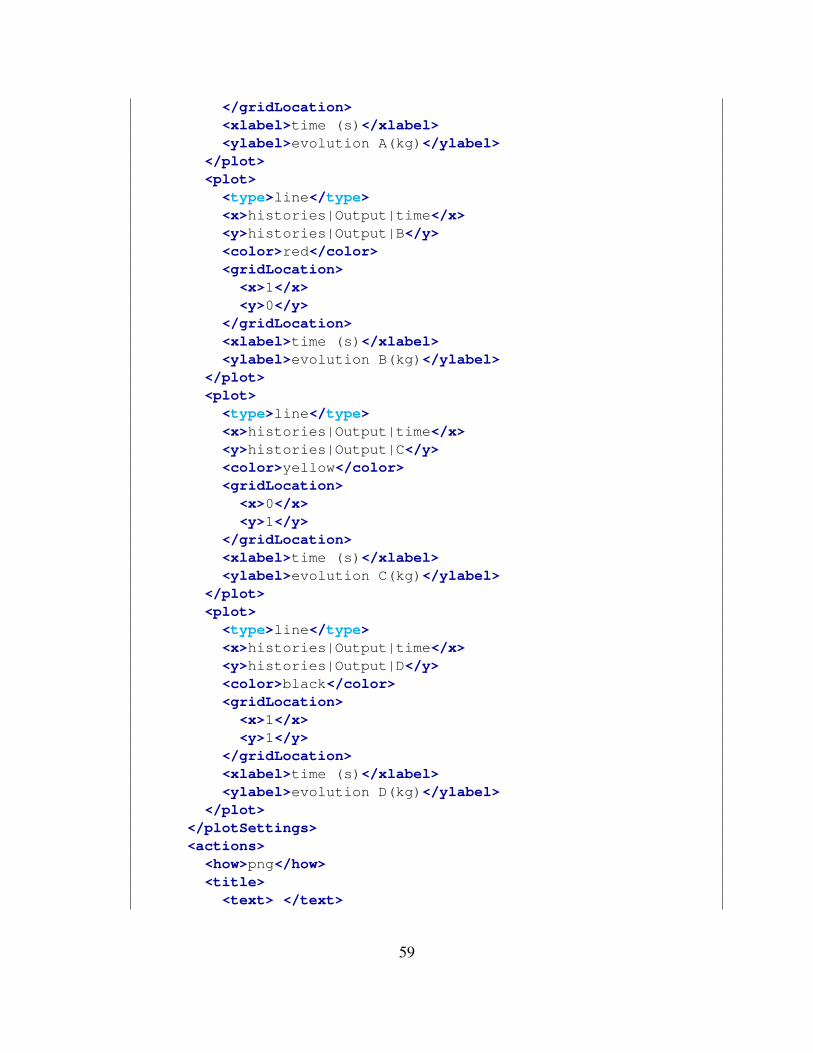
</gridLocation><xlabel>time (s)</xlabel><ylabel>evolution A(kg)</ylabel>
</plot><plot>
<type>line</type><x>histories|Output|time</x><y>histories|Output|B</y><color>red</color><gridLocation>
<x>1</x><y>0</y>
</gridLocation><xlabel>time (s)</xlabel><ylabel>evolution B(kg)</ylabel>
</plot><plot>
<type>line</type><x>histories|Output|time</x><y>histories|Output|C</y><color>yellow</color><gridLocation>
<x>0</x><y>1</y>
</gridLocation><xlabel>time (s)</xlabel><ylabel>evolution C(kg)</ylabel>
</plot><plot>
<type>line</type><x>histories|Output|time</x><y>histories|Output|D</y><color>black</color><gridLocation>
<x>1</x><y>1</y>
</gridLocation><xlabel>time (s)</xlabel><ylabel>evolution D(kg)</ylabel>
</plot></plotSettings><actions>
<how>png</how><title>
<text> </text>
59
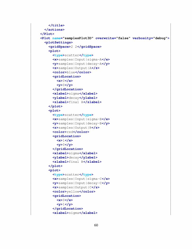
</title></actions>
</Plot><Plot name="samplesPlot3D" overwrite="false" verbosity="debug"><plotSettings>
<gridSpace>2 2</gridSpace><plot>
<type>scatter</type><x>samples|Input|sigma-A</x><y>samples|Input|decay-A</y><z>samples|Output|A</z><color>blue</color><gridLocation>
<x>0</x><y>0</y>
</gridLocation><xlabel>sigma</xlabel><ylabel>decay</ylabel><zlabel>final A</zlabel>
</plot><plot>
<type>scatter</type><x>samples|Input|sigma-B</x><y>samples|Input|decay-B</y><z>samples|Output|B</z><color>red</color><gridLocation>
<x>1</x><y>0</y>
</gridLocation><xlabel>sigma</xlabel><ylabel>decay</ylabel><zlabel>final B</zlabel>
</plot><plot>
<type>scatter</type><x>samples|Input|sigma-C</x><y>samples|Input|decay-C</y><z>samples|Output|C</z><color>yellow</color><gridLocation>
<x>0</x><y>1</y>
</gridLocation><xlabel>sigma</xlabel>
60

<ylabel>decay</ylabel><zlabel>final C</zlabel>
</plot><plot>
<type>scatter</type><x>samples|Input|sigma-D</x><y>samples|Input|decay-D</y><z>samples|Output|D</z><color>black</color><gridLocation>
<x>1</x><y>1</y>
</gridLocation><xlabel>sigma</xlabel><ylabel>decay</ylabel><zlabel>final D</zlabel>
</plot><xlabel>sigma</xlabel><ylabel>decay</ylabel><zlabel>final response</zlabel>
</plotSettings><actions>
<how>png</how><title>
<text> </text></title>
</actions></Plot>
</OutStreams>...
</Simulation>
To see the results of the simulation, <OutStreams> are included in the input. In this block,both OutStream types are used:
• Print:
– “samples” connected with the DataObjects Entity “samples” (<source>)– “histories” connected with the DataObjects Entity “histories” (<source>)
Note that in RAVEN, multiple entities can have the same name, as it takes a class,a type, and a name to uniquely identify a RAVEN object. When the two OutStreamobjects are used, all the information contained in the linked DataObjects are going tobe exported in CSV files (<type>).
• Plot:
61
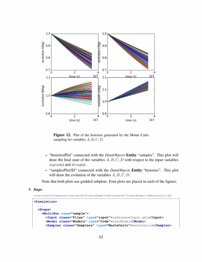
Figure 12. Plot of the histories generated by the Monte Carlosampling for variables A,B,C,D.
– “historiesPlot” connected with the DataObjects Entity “samples”. This plot willdraw the final state of the variables A,B,C,D with respect to the input variablessigma(s) and decay(s) .
– “samplesPlot3D” connected with the DataObjects Entity “histories”. This plotwill draw the evolution of the variables A,B,C,D.
Note that both plots use gridded subplots. Four plots are placed in each of the figures.
8. Steps:raven/tests/framework/user guide/ForwardSamplingStrategies/forwardSamplingMontecarlo.xml
<Simulation>...<Steps>
<MultiRun name="sample"><Input class="Files" type="input">referenceInput.xml</Input><Model class="Models" type="Code">testModel</Model><Sampler class="Samplers" type="MonteCarlo">monteCarlo</Sampler>
62

<Output class="DataObjects" type="PointSet">samples</Output><Output class="DataObjects" type="HistorySet">histories</Output>
</MultiRun><IOStep name="writeHistories" pauseAtEnd="True"><Input class="DataObjects" type="HistorySet">histories</Input><Input class="DataObjects" type="PointSet">samples</Input><Output class="OutStreams" type="Plot">samplesPlot3D</Output><Output class="OutStreams" type="Plot">historyPlot</Output><Output class="OutStreams" type="Print">samples</Output><Output class="OutStreams" type="Print">histories</Output>
</IOStep></Steps>...
</Simulation>
Figure 13. Plot of the samples generated by the MC sampling forvariables A,B,C,D.
Once all the other entities are defined in the RAVEN input file, they must be combined in the<Steps> block, which dictates the workflow of RAVEN. For this case, two <Steps> aredefined:
63

• <MultiRun> “sample”, used to run the multiple instances of the driven code andcollect the outputs in the two DataObjects. As it can be seen, the <Sampler> isspecified to communicate to the Step that the driven code needs to be perturbed throughthe Monte-Carlo sampling.
• <IOStep> named “writeHistories”, used to 1) dump the “histories” and “samples”DataObjects Entity to a CSV file and 2) plot the data in the EPS file.
Figures 12 and 13 show the report generated by RAVEN of the evolution of the variablesA,B,C,Dand their final values, respectively.
3.2 Grid sampling through RAVEN
The Grid sampling method (also known as Full Factorial Design of Experiment) represents one ofthe simplest methodologies that can be employed in order to explore the interaction of multiplerandom variables with respect selected FOMs. The goal of this section is to show how to:
1. Set up a simple Grid sampling for performing a parametric analysis of a driven code
2. Load the outputs of the code into the RAVEN DataObjects system
3. Print out what contained in the DataObjects
4. Generate basic plots of the code result.
In order to accomplish these tasks, the following RAVEN Entities (XML blocks in the input files)are required:
1. RunInfo:
raven/tests/framework/user guide/ForwardSamplingStrategies/forwardSamplingGrid.xml
<Simulation>...<RunInfo>
<JobName>RunDir/Grid</JobName><Sequence>sample,writeHistories</Sequence><WorkingDir>RunDir/Grid</WorkingDir><batchSize>2</batchSize>
</RunInfo>...
</Simulation>
64

As shown in Section ??, the RunInfo Entity is intended to set up the desired analysis.In this specific case, two steps (<Sequence>) are sequentially run using 12 processors(<batchSize>). This means that 12 instances of the driven code are run simultaneously.Every time a simulation ends, a new one is launched.
2. Files:raven/tests/framework/user guide/ForwardSamplingStrategies/forwardSamplingGrid.xml
<Simulation>...<Files>
<Input name="referenceInput.xml"type="input">referenceInput.xml</Input>
</Files>...
</Simulation>
Since the driven code uses a single input file, in this section the original input is placed. Asdescribed in the user manual [4] the attribute name represents the alias that is used in all theother input blocks in order to refer to this file.
3. Models:raven/tests/framework/user guide/ForwardSamplingStrategies/forwardSamplingGrid.xml
<Simulation>...<Models><Code name="testModel" subType="GenericCode">
<executable>../physicalCode/analyticalbateman/AnalyticalDplMain.py</executable><clargs arg="python" type="prepend" /><clargs arg="" extension=".xml" type="input" /><clargs arg=" " extension=".csv" type="output" />
</Code></Models>...
</Simulation>
The Model here is represented by the AnalyticalBateman, which already dumps its outputfile in a CSV format (standard format that RAVEN can read). For this reason, the Generic-Code interface is used.
4. Distributions:
raven/tests/framework/user guide/ForwardSamplingStrategies/forwardSamplingGrid.xml
<Simulation>...<Distributions>
<Uniform name="sigma"><lowerBound>1</lowerBound><upperBound>10</upperBound>
65

</Uniform><Uniform name="decayConstant">
<lowerBound>0.000000005</lowerBound><upperBound>0.000000010</upperBound>
</Uniform></Distributions>...
</Simulation>
In the Distributions XML section, the stochastic model for the uncertainties treated by theGrid sampling are reported. In this case two distributions are defined:
• sigma ∼ U(1, 10), used to model the uncertainties associated with the Model sigma(s)
• decayConstant ∼ U(0.5e−8, 1e−8), used to model the uncertainties associated withthe Model decay constants.
5. Samplers:raven/tests/framework/user guide/ForwardSamplingStrategies/forwardSamplingGrid.xml
<Simulation>...<Samplers><Grid name="grid">
<variable name="sigma-A"><distribution>sigma</distribution><grid construction="equal" steps="1" type="value">2 4.0</grid>
</variable><variable name="decay-A">
<distribution>decayConstant</distribution><grid construction="custom" type="value">0.000000005 0.000000008</grid>
</variable><variable name="sigma-B">
<distribution>sigma</distribution><grid construction="equal" steps="1" type="CDF">0.1 0.8</grid>
</variable><variable name="decay-B">
<distribution>decayConstant</distribution><grid construction="equal" steps="1" type="CDF">0.1 0.8</grid>
</variable><variable name="sigma-C">
<distribution>sigma</distribution><grid construction="equal" steps="1" type="value">4 5</grid>
</variable><variable name="decay-C">
<distribution>decayConstant</distribution><grid construction="equal" steps="1" type="CDF">0.1 0.5</grid>
</variable><variable name="sigma-D">
<distribution>sigma</distribution><grid construction="equal" steps="1" type="CDF">0.4 0.8</grid>
</variable><variable name="decay-D">
<distribution>decayConstant</distribution><grid construction="equal" steps="1" type="CDF">0.1 0.8</grid>
</variable></Grid>
</Samplers>
66

...</Simulation>
To employ the Grid sampling strategy, a <Grid> node needs to be specified. As shownabove, in each variable section, the <grid> is defined. The number of samples finallyrequested are equal to nsamples =
∏ni=1 nstepsi+1 = 256. Note that, for each variable, can be
defined either in probability (CDF) or in absolute value.
6. DataObjects:raven/tests/framework/user guide/ForwardSamplingStrategies/forwardSamplingGrid.xml
<Simulation>...<DataObjects><PointSet name="samples">
<Input>sigma-A,sigma-B,sigma-C,sigma-D,decay-A,decay-B,decay-C,decay-D</Input><Output>A,B,C,D,time</Output>
</PointSet><HistorySet name="histories">
<Input>sigma-A,sigma-B,sigma-C,sigma-D,decay-A,decay-B,decay-C,decay-D</Input><Output>A,B,C,D,time</Output>
</HistorySet></DataObjects>...
</Simulation>
Int this block, two DataObjects are defined: 1) PointSet named “samples”, and 2) HistorySetnamed “histories”. In the <Input> node all the variables perturbed through the Grid strat-egy are listed. In this way, any realization in the input space is linked to the outputs listed inthe <Output> node.
7. OutStreams:
raven/tests/framework/user guide/ForwardSamplingStrategies/forwardSamplingGrid.xml
<Simulation>...<OutStreams><Print name="samples"><type>csv</type><source>samples</source>
</Print><Print name="histories"><type>csv</type><source>histories</source>
</Print><Plot name="historyPlot" overwrite="false" verbosity="debug"><plotSettings>
<gridSpace>2 2</gridSpace><plot>
<type>line</type><x>histories|Output|time</x>
67
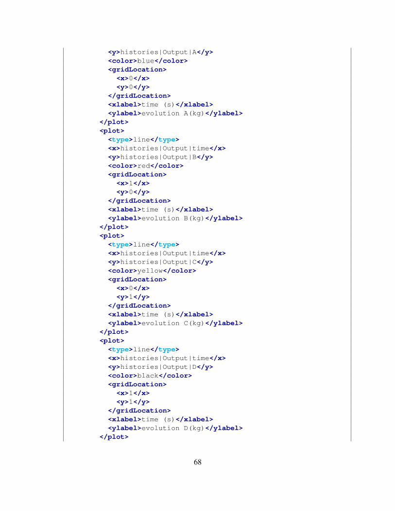
<y>histories|Output|A</y><color>blue</color><gridLocation>
<x>0</x><y>0</y>
</gridLocation><xlabel>time (s)</xlabel><ylabel>evolution A(kg)</ylabel>
</plot><plot>
<type>line</type><x>histories|Output|time</x><y>histories|Output|B</y><color>red</color><gridLocation>
<x>1</x><y>0</y>
</gridLocation><xlabel>time (s)</xlabel><ylabel>evolution B(kg)</ylabel>
</plot><plot>
<type>line</type><x>histories|Output|time</x><y>histories|Output|C</y><color>yellow</color><gridLocation>
<x>0</x><y>1</y>
</gridLocation><xlabel>time (s)</xlabel><ylabel>evolution C(kg)</ylabel>
</plot><plot>
<type>line</type><x>histories|Output|time</x><y>histories|Output|D</y><color>black</color><gridLocation>
<x>1</x><y>1</y>
</gridLocation><xlabel>time (s)</xlabel><ylabel>evolution D(kg)</ylabel>
</plot>
68
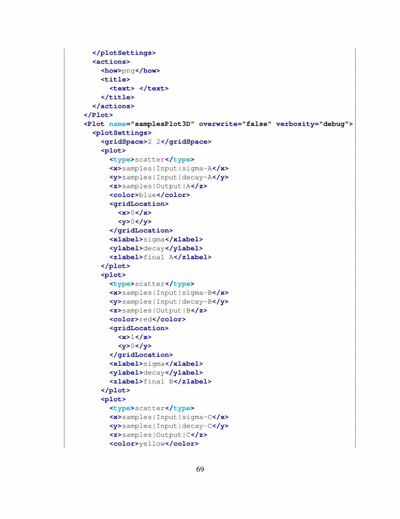
</plotSettings><actions>
<how>png</how><title>
<text> </text></title>
</actions></Plot><Plot name="samplesPlot3D" overwrite="false" verbosity="debug"><plotSettings>
<gridSpace>2 2</gridSpace><plot>
<type>scatter</type><x>samples|Input|sigma-A</x><y>samples|Input|decay-A</y><z>samples|Output|A</z><color>blue</color><gridLocation>
<x>0</x><y>0</y>
</gridLocation><xlabel>sigma</xlabel><ylabel>decay</ylabel><zlabel>final A</zlabel>
</plot><plot>
<type>scatter</type><x>samples|Input|sigma-B</x><y>samples|Input|decay-B</y><z>samples|Output|B</z><color>red</color><gridLocation>
<x>1</x><y>0</y>
</gridLocation><xlabel>sigma</xlabel><ylabel>decay</ylabel><zlabel>final B</zlabel>
</plot><plot>
<type>scatter</type><x>samples|Input|sigma-C</x><y>samples|Input|decay-C</y><z>samples|Output|C</z><color>yellow</color>
69

<gridLocation><x>0</x><y>1</y>
</gridLocation><xlabel>sigma</xlabel><ylabel>decay</ylabel><zlabel>final C</zlabel>
</plot><plot>
<type>scatter</type><x>samples|Input|sigma-D</x><y>samples|Input|decay-D</y><z>samples|Output|D</z><color>black</color><gridLocation>
<x>1</x><y>1</y>
</gridLocation><xlabel>sigma</xlabel><ylabel>decay</ylabel><zlabel>final D</zlabel>
</plot><xlabel>sigma</xlabel><ylabel>decay</ylabel><zlabel>final response</zlabel>
</plotSettings><actions>
<how>png</how><title>
<text> </text></title>
</actions></Plot>
</OutStreams>...
</Simulation>
In this block, both the Out-Stream types are constructed:
• Print:
– named “samples” connected with the DataObjects Entity “samples” (<source>)– named “histories” connected with the DataObjects Entity “histories” (<source>).
When these objects get used, all the information contained in the linked DataObjectsare going to be exported in CSV files (<type>).
70

Figure 14. Plot of the histories generated by the Grid samplingfor variables A,B,C,D.
• Plot:
– named “historiesPlot” connected with the DataObjects Entity “samples”. Thisplot will draw the final state of the variables A,B,C,D with respect to the inputvariables sigma(s) and decay(s).
– named “samplesPlot3D” connected with the DataObjects Entity “histories”. Thisplot will draw the evolution of the variables A,B,C,D.
As it can be noticed, both plots are of type SubPlot. Four plots are placed in each ofthe figures.
8. Steps:raven/tests/framework/user guide/ForwardSamplingStrategies/forwardSamplingGrid.xml
<Simulation>...<Steps>
<MultiRun name="sample"><Input class="Files" type="input">referenceInput.xml</Input>
71

<Model class="Models" type="Code">testModel</Model><Sampler class="Samplers" type="Grid">grid</Sampler><Output class="DataObjects" type="PointSet">samples</Output><Output class="DataObjects" type="HistorySet">histories</Output>
</MultiRun><IOStep name="writeHistories" pauseAtEnd="True"><Input class="DataObjects" type="HistorySet">histories</Input><Input class="DataObjects" type="PointSet">samples</Input><Output class="OutStreams" type="Plot">samplesPlot3D</Output><Output class="OutStreams" type="Plot">historyPlot</Output><Output class="OutStreams" type="Print">samples</Output><Output class="OutStreams" type="Print">histories</Output>
</IOStep></Steps>...
</Simulation>
Figure 15. Plot of the samples generated by the Grid samplingfor variables A,B,C,D.
Finally, all the previously defined Entities can be combined in the <Steps> block. Asinferable, two <Steps> have been inputted:
72
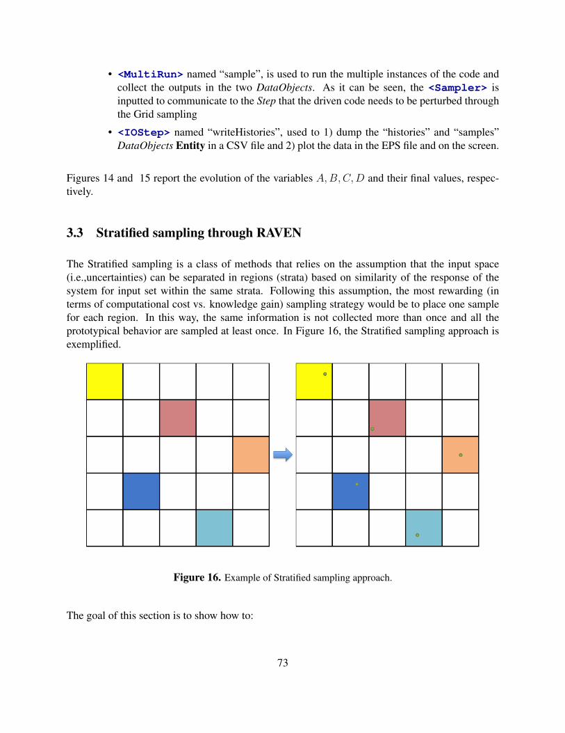
• <MultiRun> named “sample”, is used to run the multiple instances of the code andcollect the outputs in the two DataObjects. As it can be seen, the <Sampler> isinputted to communicate to the Step that the driven code needs to be perturbed throughthe Grid sampling
• <IOStep> named “writeHistories”, used to 1) dump the “histories” and “samples”DataObjects Entity in a CSV file and 2) plot the data in the EPS file and on the screen.
Figures 14 and 15 report the evolution of the variables A,B,C,D and their final values, respec-tively.
3.3 Stratified sampling through RAVEN
The Stratified sampling is a class of methods that relies on the assumption that the input space(i.e.,uncertainties) can be separated in regions (strata) based on similarity of the response of thesystem for input set within the same strata. Following this assumption, the most rewarding (interms of computational cost vs. knowledge gain) sampling strategy would be to place one samplefor each region. In this way, the same information is not collected more than once and all theprototypical behavior are sampled at least once. In Figure 16, the Stratified sampling approach isexemplified.
Figure 16. Example of Stratified sampling approach.
The goal of this section is to show how to:
73
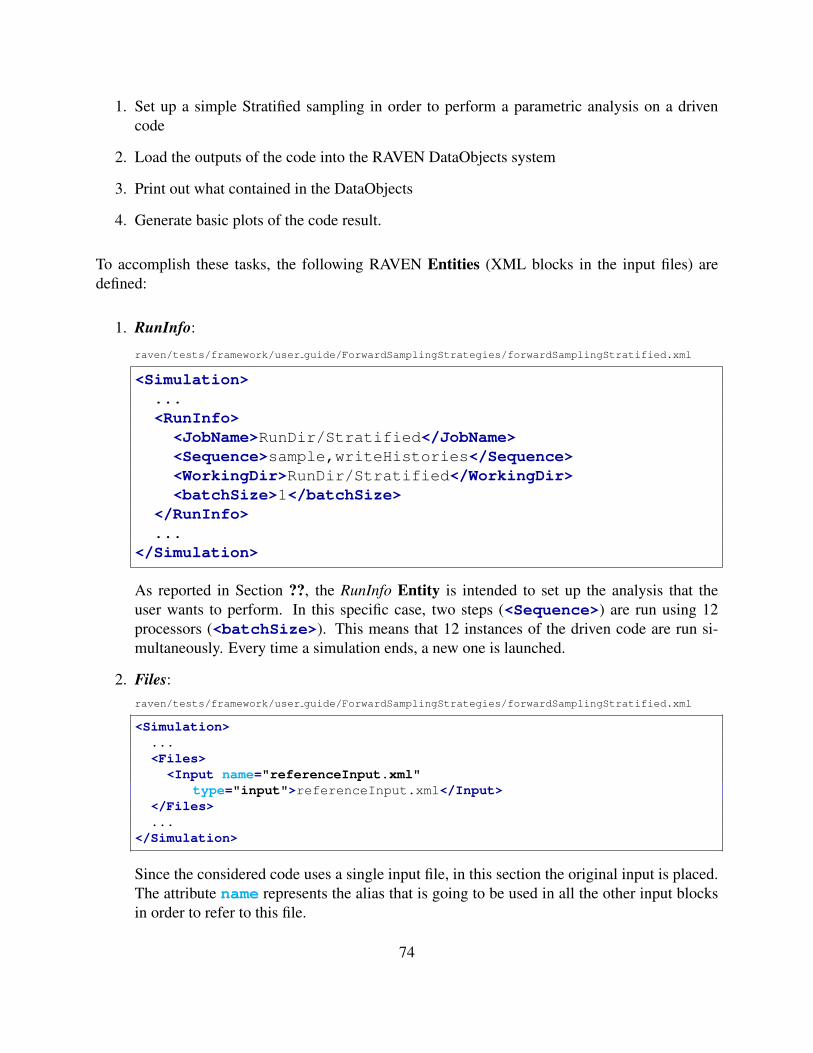
1. Set up a simple Stratified sampling in order to perform a parametric analysis on a drivencode
2. Load the outputs of the code into the RAVEN DataObjects system
3. Print out what contained in the DataObjects
4. Generate basic plots of the code result.
To accomplish these tasks, the following RAVEN Entities (XML blocks in the input files) aredefined:
1. RunInfo:
raven/tests/framework/user guide/ForwardSamplingStrategies/forwardSamplingStratified.xml
<Simulation>...<RunInfo>
<JobName>RunDir/Stratified</JobName><Sequence>sample,writeHistories</Sequence><WorkingDir>RunDir/Stratified</WorkingDir><batchSize>1</batchSize>
</RunInfo>...
</Simulation>
As reported in Section ??, the RunInfo Entity is intended to set up the analysis that theuser wants to perform. In this specific case, two steps (<Sequence>) are run using 12processors (<batchSize>). This means that 12 instances of the driven code are run si-multaneously. Every time a simulation ends, a new one is launched.
2. Files:raven/tests/framework/user guide/ForwardSamplingStrategies/forwardSamplingStratified.xml
<Simulation>...<Files>
<Input name="referenceInput.xml"type="input">referenceInput.xml</Input>
</Files>...
</Simulation>
Since the considered code uses a single input file, in this section the original input is placed.The attribute name represents the alias that is going to be used in all the other input blocksin order to refer to this file.
74

3. Models:raven/tests/framework/user guide/ForwardSamplingStrategies/forwardSamplingStratified.xml
<Simulation>...<Models><Code name="testModel" subType="GenericCode">
<executable>../physicalCode/analyticalbateman/AnalyticalDplMain.py</executable><clargs arg="python" type="prepend" /><clargs arg="" extension=".xml" type="input" /><clargs arg=" " extension=".csv" type="output" />
</Code></Models>...
</Simulation>
The Model here is represented by the AnalyticalBateman, which already dumps its outputfile in a CSV format (standard format that RAVEN can read). For this reason, the Generic-Code interface is used.
4. Distributions:
raven/tests/framework/user guide/ForwardSamplingStrategies/forwardSamplingStratified.xml
<Simulation>...<Distributions>
<Uniform name="sigma"><lowerBound>1</lowerBound><upperBound>10</upperBound>
</Uniform><Uniform name="decayConstant">
<lowerBound>0.000000005</lowerBound><upperBound>0.000000010</upperBound>
</Uniform></Distributions>...
</Simulation>
In the Distributions XML section, the stochastic model for the uncertainties treated by theStratified sampling are reported. In this case two distributions are defined:
• sigma ∼ U(1, 10), used to model the uncertainties associated with the Model sigma(s)
• decayConstant ∼ U(0.5e−8, 1e−8), used to model the uncertainties associated withthe Model decay constants.
5. Samplers:raven/tests/framework/user guide/ForwardSamplingStrategies/forwardSamplingStratified.xml
75

<Simulation>...<Samplers><Stratified name="stratified">
<samplerInit><initialSeed>42</initialSeed>
</samplerInit><variable name="sigma-A">
<distribution>sigma</distribution><grid construction="equal" steps="100" type="value">2 4.0</grid>
</variable><variable name="decay-A">
<distribution>decayConstant</distribution><grid construction="equal" steps="100" type="value">0.000000005 0.000000008</grid>
</variable><variable name="sigma-B">
<distribution>sigma</distribution><grid construction="equal" steps="100" type="CDF">0.1 0.8</grid>
</variable><variable name="decay-B">
<distribution>decayConstant</distribution><grid construction="equal" steps="100" type="CDF">0.1 0.8</grid>
</variable><variable name="sigma-C">
<distribution>sigma</distribution><grid construction="equal" steps="100" type="value">1.0 5</grid>
</variable><variable name="decay-C">
<distribution>decayConstant</distribution><grid construction="equal" steps="100" type="CDF">0.1 0.5</grid>
</variable><variable name="sigma-D">
<distribution>sigma</distribution><grid construction="equal" steps="100" type="CDF">0.4 0.8</grid>
</variable><variable name="decay-D">
<distribution>decayConstant</distribution><grid construction="equal" steps="100" type="CDF">0.1 0.8</grid>
</variable></Stratified>
</Samplers>...
</Simulation>
To employ the Stratified sampling strategy, a <Stratified> node needs to be specified.In each variable section, the <grid> is defined. It is important to mention that the number ofsteps needs to be the same for each of the variables, since, as reported in previous section,the Stratified sampling strategy it discretizes the domain in strata. The number of samplesfinally requested is equal to nsamples = nsteps = 100. If the grid for each variables is definedin CDF and of type = “equal”, the Stratified sampling corresponds to the well-known LatinHyper Cube sampling.
6. DataObjects:raven/tests/framework/user guide/ForwardSamplingStrategies/forwardSamplingStratified.xml
<Simulation>...<DataObjects><PointSet name="samples">
76

<Input>sigma-A,sigma-B,sigma-C,sigma-D,decay-A,decay-B,decay-C,decay-D</Input><Output>A,B,C,D,time</Output>
</PointSet><HistorySet name="histories">
<Input>sigma-A,sigma-B,sigma-C,sigma-D,decay-A,decay-B,decay-C,decay-D</Input><Output>A,B,C,D,time</Output>
</HistorySet></DataObjects>...
</Simulation>
In this block, two DataObjects are defined: 1) PointSet named “samples”, 2) HistorySetnamed “histories”. In the <Input> node all the variables perturbed through the Stratifiedstrategy are listed. In this way, any realization in the input space is linked to the outputslisted in the <Output> node.
7. OutStreams:
raven/tests/framework/user guide/ForwardSamplingStrategies/forwardSamplingStratified.xml
<Simulation>...<OutStreams><Print name="samples"><type>csv</type><source>samples</source>
</Print><Print name="histories"><type>csv</type><source>histories</source>
</Print><Plot name="historyPlot" overwrite="false" verbosity="debug"><plotSettings>
<gridSpace>2 2</gridSpace><plot>
<type>line</type><x>histories|Output|time</x><y>histories|Output|A</y><color>blue</color><gridLocation>
<x>0</x><y>0</y>
</gridLocation><xlabel>time (s)</xlabel><ylabel>evolution A(kg)</ylabel>
</plot><plot>
<type>line</type><x>histories|Output|time</x>
77

<y>histories|Output|B</y><color>red</color><gridLocation>
<x>1</x><y>0</y>
</gridLocation><xlabel>time (s)</xlabel><ylabel>evolution B(kg)</ylabel>
</plot><plot>
<type>line</type><x>histories|Output|time</x><y>histories|Output|C</y><color>yellow</color><gridLocation>
<x>0</x><y>1</y>
</gridLocation><xlabel>time (s)</xlabel><ylabel>evolution C(kg)</ylabel>
</plot><plot>
<type>line</type><x>histories|Output|time</x><y>histories|Output|D</y><color>black</color><gridLocation>
<x>1</x><y>1</y>
</gridLocation><xlabel>time (s)</xlabel><ylabel>evolution D(kg)</ylabel>
</plot></plotSettings><actions>
<how>png</how><title>
<text> </text></title>
</actions></Plot><Plot name="samplesPlot3D" overwrite="false" verbosity="debug"><plotSettings>
<gridSpace>2 2</gridSpace><plot>
78
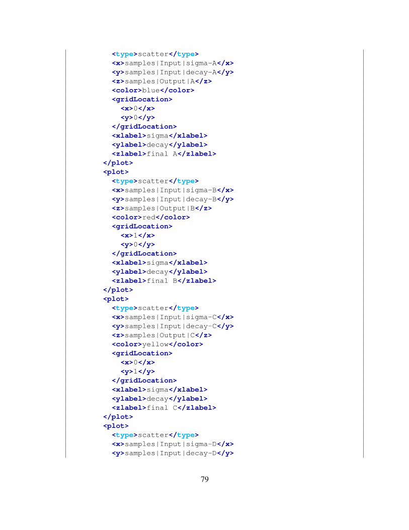
<type>scatter</type><x>samples|Input|sigma-A</x><y>samples|Input|decay-A</y><z>samples|Output|A</z><color>blue</color><gridLocation>
<x>0</x><y>0</y>
</gridLocation><xlabel>sigma</xlabel><ylabel>decay</ylabel><zlabel>final A</zlabel>
</plot><plot>
<type>scatter</type><x>samples|Input|sigma-B</x><y>samples|Input|decay-B</y><z>samples|Output|B</z><color>red</color><gridLocation>
<x>1</x><y>0</y>
</gridLocation><xlabel>sigma</xlabel><ylabel>decay</ylabel><zlabel>final B</zlabel>
</plot><plot>
<type>scatter</type><x>samples|Input|sigma-C</x><y>samples|Input|decay-C</y><z>samples|Output|C</z><color>yellow</color><gridLocation>
<x>0</x><y>1</y>
</gridLocation><xlabel>sigma</xlabel><ylabel>decay</ylabel><zlabel>final C</zlabel>
</plot><plot>
<type>scatter</type><x>samples|Input|sigma-D</x><y>samples|Input|decay-D</y>
79

<z>samples|Output|D</z><color>black</color><gridLocation>
<x>1</x><y>1</y>
</gridLocation><xlabel>sigma</xlabel><ylabel>decay</ylabel><zlabel>final D</zlabel>
</plot><xlabel>sigma</xlabel><ylabel>decay</ylabel><zlabel>final response</zlabel>
</plotSettings><actions>
<how>png</how><title>
<text> </text></title>
</actions></Plot>
</OutStreams>...
</Simulation>
In this block, both the Out-Stream types are constructed:
• Print:
– named “samples” connected with the DataObjects Entity “samples” (<source>)– named “histories” connected with the DataObjects Entity “histories” (<source>).
When these objects get used, all the information contained in the linked DataObjectsare going to be exported in CSV files (<type>).
• Plot:
– named “historiesPlot” connected with the DataObjects Entity “samples”. Thisplot will draw the final state of the variables A,B,C,D with respect to the inputvariables sigma(s) and decay(s)
– named “samplesPlot3D” connected with the DataObjects Entity “histories”. Thisplot will draw the evolution of the variables A,B,C,D.
As it can be noticed, both plots are of type SubPlot. Four plots are going to be placedin each of the figures.
8. Steps:
80
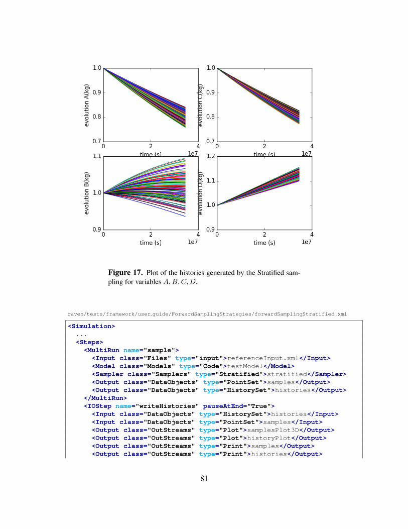
Figure 17. Plot of the histories generated by the Stratified sam-pling for variables A,B,C,D.
raven/tests/framework/user guide/ForwardSamplingStrategies/forwardSamplingStratified.xml
<Simulation>...<Steps>
<MultiRun name="sample"><Input class="Files" type="input">referenceInput.xml</Input><Model class="Models" type="Code">testModel</Model><Sampler class="Samplers" type="Stratified">stratified</Sampler><Output class="DataObjects" type="PointSet">samples</Output><Output class="DataObjects" type="HistorySet">histories</Output>
</MultiRun><IOStep name="writeHistories" pauseAtEnd="True"><Input class="DataObjects" type="HistorySet">histories</Input><Input class="DataObjects" type="PointSet">samples</Input><Output class="OutStreams" type="Plot">samplesPlot3D</Output><Output class="OutStreams" type="Plot">historyPlot</Output><Output class="OutStreams" type="Print">samples</Output><Output class="OutStreams" type="Print">histories</Output>
81
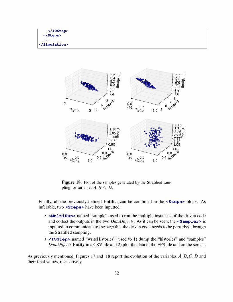
</IOStep></Steps>...
</Simulation>
Figure 18. Plot of the samples generated by the Stratified sam-pling for variables A,B,C,D.
Finally, all the previously defined Entities can be combined in the <Steps> block. Asinferable, two <Steps> have been inputted:
• <MultiRun> named “sample”, used to run the multiple instances of the driven codeand collect the outputs in the two DataObjects. As it can be seen, the <Sampler> isinputted to communicate to the Step that the driven code needs to be perturbed throughthe Stratified sampling.
• <IOStep> named “writeHistories”, used to 1) dump the “histories” and “samples”DataObjects Entity in a CSV file and 2) plot the data in the EPS file and on the screen.
As previously mentioned, Figures 17 and 18 report the evolution of the variables A,B,C,D andtheir final values, respectively.
82

3.4 Sparse Grid Collocation sampling through RAVEN
The Sparse Grid Collocation sampler represents an advanced methodology to perform UncertaintyQuantification. They aim to explore the input space leveraging the information contained in theassociated probability density functions. It builds on generic Grid sampling by selecting evaluationpoints based on characteristic quadratures as part of stochastic collocation for generalized polyno-mial chaos uncertainty quantification. In collocation an N-D grid is constructed, with each uncer-tain variable providing an axis. Along each axis, the points of evaluation correspond to quadraturepoints necessary to integrate polynomials. In the simplest (and most naive) case, a N-D tensorproduct of all possible combinations of points from each dimension’s quadrature is constructed assampling points. The number of necessary samples can be reduced by employing Smolyak-likesparse grid algorithms, which use reduced combinations of polynomial orders to reduce the neces-sary sampling space.The goals of this section are about learning how to:
1. Set up a Sparse Grid Collocation sampling for the construction of a suitable surrogate modelof a driven code
2. Construct a GaussPolynomialRom surrogate model (training stage)
3. Use the constructed GaussPolynomialRom surrogate model instead of the driven code.
To accomplish these tasks, the following RAVEN Entities (XML blocks in the input files) need tobe defined:
1. RunInfo:raven/tests/framework/user guide/ForwardSamplingStrategies/forwardSamplingSparseGrid.xml
<Simulation>...<RunInfo><JobName>RunDir/SparseGrid</JobName><WorkingDir>RunDir/SparseGrid</WorkingDir><Sequence>sample,train,validateModel,validateROM,output_print,output_plot</Sequence><batchSize>8</batchSize>
</RunInfo>...
</Simulation>
As reported in section ??, the RunInfo Entity is intended to set up the analysis that the userwants to perform. In this specific case, six steps (<Sequence>) are going to be sequen-tially run using twelve processors (<batchSize>). The first two steps build the ROM(’sample’, ’train’), the next two validate the ROM against the original Code Model(’validateModel’, ’validateROM’), and the last two produce plots and print data(’output print’, ’output plot’).
83
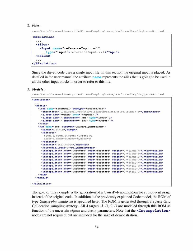
2. Files:raven/tests/framework/user guide/ForwardSamplingStrategies/forwardSamplingSparseGrid.xml
<Simulation>...<Files>
<Input name="referenceInput.xml"type="input">referenceInput.xml</Input>
</Files>...
</Simulation>
Since the driven code uses a single input file, in this section the original input is placed. Asdetailed in the user manual the attribute name represents the alias that is going to be used inall the other input blocks in order to refer to this file.
3. Models:raven/tests/framework/user guide/ForwardSamplingStrategies/forwardSamplingSparseGrid.xml
<Simulation>...<Models><Code name="testModel" subType="GenericCode">
<executable>../physicalCode/analyticalbateman/AnalyticalDplMain.py</executable><clargs arg="python" type="prepend" /><clargs arg="" extension=".xml" type="input" /><clargs arg="" extension=".csv" type="output" />
</Code><ROM name="rom" subType="GaussPolynomialRom">
<Target>A,B,C,D</Target><Features>
sigma-A,sigma-B,sigma-C,sigma-D,decay-A,decay-B,decay-C,decay-D
</Features><IndexSet>TotalDegree</IndexSet><PolynomialOrder>2</PolynomialOrder><Interpolation poly="Legendre" quad="Legendre" weight="1">sigma-A</Interpolation><Interpolation poly="Legendre" quad="Legendre" weight="1">sigma-B</Interpolation><Interpolation poly="Legendre" quad="Legendre" weight="1">sigma-C</Interpolation><Interpolation poly="Legendre" quad="Legendre" weight="1">sigma-D</Interpolation><Interpolation poly="Legendre" quad="Legendre" weight="1">decay-A</Interpolation><Interpolation poly="Legendre" quad="Legendre" weight="1">decay-B</Interpolation><Interpolation poly="Legendre" quad="Legendre" weight="1">decay-C</Interpolation><Interpolation poly="Legendre" quad="Legendre" weight="1">decay-D</Interpolation>
</ROM></Models>...
</Simulation>
The goal of this example is the generation of a GaussPolynomialRom for subsequent usageinstead of the original code. In addition to the previously explained Code model, the ROM oftype GaussPolynomialRom is specified here. The ROM is generated through a Sparse GridCollocation sampling strategy. All 4 targets A,B,C,D are modeled through this ROM asfunction of the uncertain sigma and decay parameters. Note that the <Interpolation>nodes are not required, but are included for the sake of demonstration.
84

4. Distributions:
raven/tests/framework/user guide/ForwardSamplingStrategies/forwardSamplingSparseGrid.xml
<Simulation>...<Distributions>
<Uniform name="sigmaA"><lowerBound>6.9</lowerBound><upperBound>8.1</upperBound>
</Uniform><Uniform name="sigmaB">
<lowerBound>3.9</lowerBound><upperBound>5.1</upperBound>
</Uniform><Uniform name="sigmaC">
<lowerBound>1.9</lowerBound><upperBound>3.1</upperBound>
</Uniform><Uniform name="sigmaD">
<lowerBound>0.9</lowerBound><upperBound>1.1</upperBound>
</Uniform><Uniform name="decayConstantA">
<lowerBound>3.8e-9</lowerBound><upperBound>5.2e-9</upperBound>
</Uniform><Uniform name="decayConstantB">
<lowerBound>5.8e-9</lowerBound><upperBound>7.2e-9</upperBound>
</Uniform><Uniform name="decayConstantC">
<lowerBound>6.8e-9</lowerBound><upperBound>8.2e-9</upperBound>
</Uniform><Uniform name="decayConstantD">
<lowerBound>7.8e-9</lowerBound><upperBound>9.2e-9</upperBound>
</Uniform></Distributions>...
</Simulation>
In the Distributions XML section, the stochastic model for the uncertainties treated by the
85
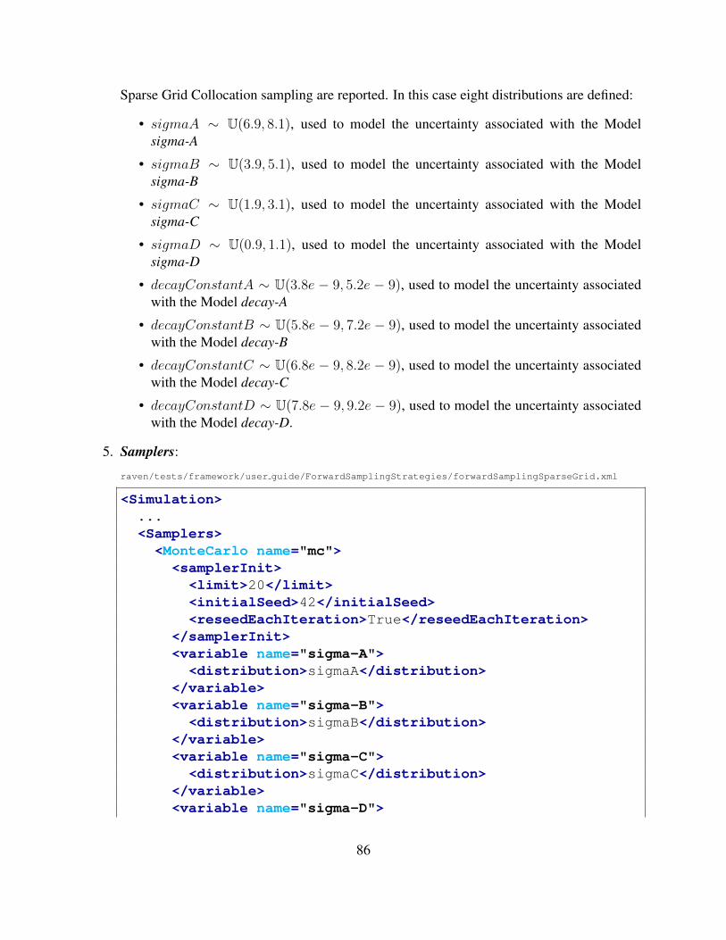
Sparse Grid Collocation sampling are reported. In this case eight distributions are defined:
• sigmaA ∼ U(6.9, 8.1), used to model the uncertainty associated with the Modelsigma-A
• sigmaB ∼ U(3.9, 5.1), used to model the uncertainty associated with the Modelsigma-B
• sigmaC ∼ U(1.9, 3.1), used to model the uncertainty associated with the Modelsigma-C
• sigmaD ∼ U(0.9, 1.1), used to model the uncertainty associated with the Modelsigma-D
• decayConstantA ∼ U(3.8e − 9, 5.2e − 9), used to model the uncertainty associatedwith the Model decay-A
• decayConstantB ∼ U(5.8e − 9, 7.2e − 9), used to model the uncertainty associatedwith the Model decay-B
• decayConstantC ∼ U(6.8e − 9, 8.2e − 9), used to model the uncertainty associatedwith the Model decay-C
• decayConstantD ∼ U(7.8e − 9, 9.2e − 9), used to model the uncertainty associatedwith the Model decay-D.
5. Samplers:
raven/tests/framework/user guide/ForwardSamplingStrategies/forwardSamplingSparseGrid.xml
<Simulation>...<Samplers>
<MonteCarlo name="mc"><samplerInit><limit>20</limit><initialSeed>42</initialSeed><reseedEachIteration>True</reseedEachIteration>
</samplerInit><variable name="sigma-A"><distribution>sigmaA</distribution>
</variable><variable name="sigma-B"><distribution>sigmaB</distribution>
</variable><variable name="sigma-C"><distribution>sigmaC</distribution>
</variable><variable name="sigma-D">
86

<distribution>sigmaD</distribution></variable><variable name="decay-A"><distribution>decayConstantA</distribution>
</variable><variable name="decay-B"><distribution>decayConstantB</distribution>
</variable><variable name="decay-C"><distribution>decayConstantC</distribution>
</variable><variable name="decay-D"><distribution>decayConstantD</distribution>
</variable></MonteCarlo><SparseGridCollocation name="SG">
<variable name="sigma-A"><distribution>sigmaA</distribution>
</variable><variable name="sigma-B"><distribution>sigmaB</distribution>
</variable><variable name="sigma-C"><distribution>sigmaC</distribution>
</variable><variable name="sigma-D"><distribution>sigmaD</distribution>
</variable><variable name="decay-A"><distribution>decayConstantA</distribution>
</variable><variable name="decay-B"><distribution>decayConstantB</distribution>
</variable><variable name="decay-C"><distribution>decayConstantC</distribution>
</variable><variable name="decay-D"><distribution>decayConstantD</distribution>
</variable><ROM class="Models" type="ROM">rom</ROM>
</SparseGridCollocation>
87

</Samplers>...
</Simulation>
In order to employ the Sparse Grid Collocation sampling strategy, a <SparseGridCollocation>node needs to be defined. As can be seen from above, each variable is associated with a dif-ferent distribution, defined in the <Distributions> block. In addition, the GaussPoly-nomialRom <ROM> is linked to the <SparseGridCollocation> sampler. Becausethis sampler is used exclusively to build the ROM, some of the parameters of the ROM areneeded by the sampler, and this connection makes that communication possible. The settingof this ROM (e.g. polynomial order, Index set method, etc.) determines how the StochasticCollocation Method is employed.
Additionally, a <MonteCarlo> sampler is set up for validating the ROM against the orig-inal Code. The random number generation seed (<initialSeed>) is specified and set toreset on each use (<reseedEachIteration>) so that the Monte Carlo sampler can beused to compare the ROM against the original model. We use twenty samples (<limit>)to sample the ROM and the model, and then print and plot both data sets to compare them.
6. DataObjects:
raven/tests/framework/user guide/ForwardSamplingStrategies/forwardSamplingSparseGrid.xml
<Simulation>...<DataObjects>
<PointSet name="inputPlaceholder"><Input>sigma-A,sigma-B,sigma-C,sigma-D,decay-A,decay-B,decay-C,decay-D
</Input><Output>OutputPlaceHolder</Output>
</PointSet><PointSet name="samplesModel">
<Input>sigma-A,sigma-B,sigma-C,sigma-D,decay-A,decay-B,decay-C,decay-D
</Input><Output>A,B,C,D</Output>
</PointSet><PointSet name="samplesROM">
<Input>sigma-A,sigma-B,sigma-C,sigma-D,decay-A,decay-B,decay-C,decay-D
</Input>
88
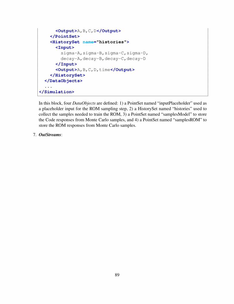
<Output>A,B,C,D</Output></PointSet><HistorySet name="histories">
<Input>sigma-A,sigma-B,sigma-C,sigma-D,decay-A,decay-B,decay-C,decay-D
</Input><Output>A,B,C,D,time</Output>
</HistorySet></DataObjects>...
</Simulation>
In this block, four DataObjects are defined: 1) a PointSet named “inputPlaceholder” used asa placeholder input for the ROM sampling step, 2) a HistorySet named “histories” used tocollect the samples needed to train the ROM, 3) a PointSet named “samplesModel” to storethe Code responses from Monte Carlo samples, and 4) a PointSet named “samplesROM” tostore the ROM responses from Monte Carlo samples.
7. OutStreams:
89
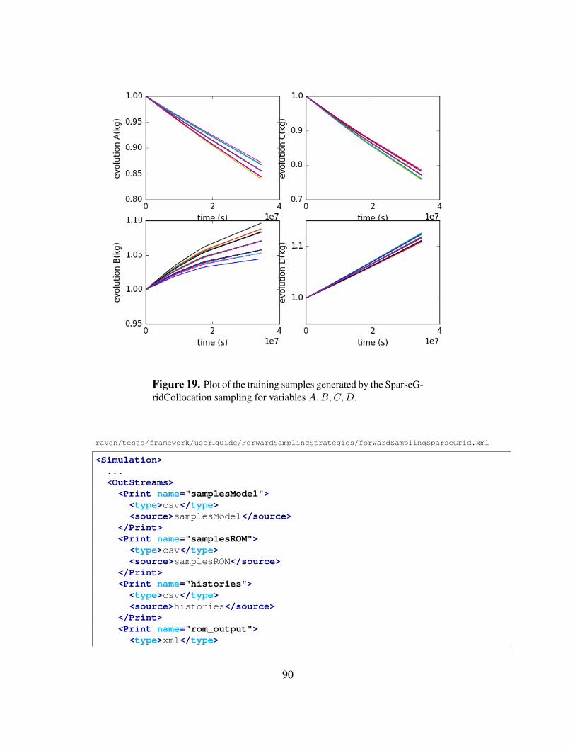
Figure 19. Plot of the training samples generated by the SparseG-ridCollocation sampling for variables A,B,C,D.
raven/tests/framework/user guide/ForwardSamplingStrategies/forwardSamplingSparseGrid.xml
<Simulation>...<OutStreams>
<Print name="samplesModel"><type>csv</type><source>samplesModel</source>
</Print><Print name="samplesROM"><type>csv</type><source>samplesROM</source>
</Print><Print name="histories"><type>csv</type><source>histories</source>
</Print><Print name="rom_output"><type>xml</type>
90

<source>rom</source><what>all</what>
</Print><Plot name="historyPlot" overwrite="false" verbosity="debug"><plotSettings>
<gridSpace>2 2</gridSpace><plot>
<type>line</type><x>histories|Output|time</x><y>histories|Output|A</y><color>blue</color><gridLocation>
<x>0</x><y>0</y>
</gridLocation><xlabel>time (s)</xlabel><ylabel>evolution A(kg)</ylabel>
</plot><plot>
<type>line</type><x>histories|Output|time</x><y>histories|Output|B</y><color>red</color><gridLocation>
<x>1</x><y>0</y>
</gridLocation><xlabel>time (s)</xlabel><ylabel>evolution B(kg)</ylabel>
</plot><plot>
<type>line</type><x>histories|Output|time</x><y>histories|Output|C</y><color>yellow</color><gridLocation>
<x>0</x><y>1</y>
</gridLocation><xlabel>time (s)</xlabel><ylabel>evolution C(kg)</ylabel>
</plot><plot>
<type>line</type><x>histories|Output|time</x><y>histories|Output|D</y><color>black</color><gridLocation>
<x>1</x><y>1</y>
</gridLocation>
91
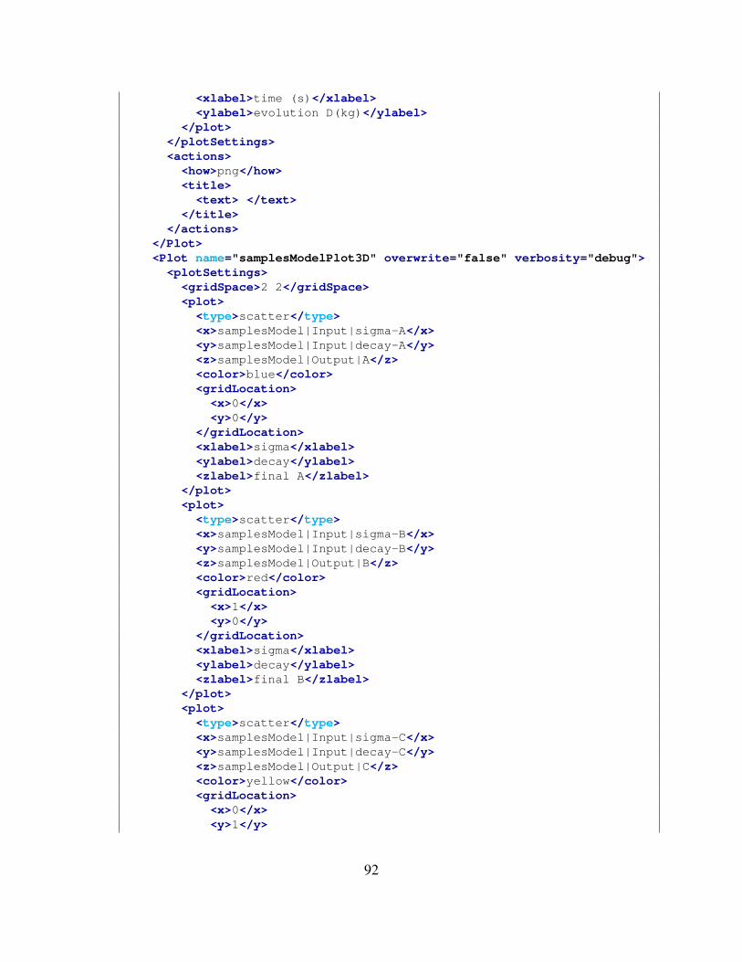
<xlabel>time (s)</xlabel><ylabel>evolution D(kg)</ylabel>
</plot></plotSettings><actions>
<how>png</how><title>
<text> </text></title>
</actions></Plot><Plot name="samplesModelPlot3D" overwrite="false" verbosity="debug"><plotSettings>
<gridSpace>2 2</gridSpace><plot>
<type>scatter</type><x>samplesModel|Input|sigma-A</x><y>samplesModel|Input|decay-A</y><z>samplesModel|Output|A</z><color>blue</color><gridLocation>
<x>0</x><y>0</y>
</gridLocation><xlabel>sigma</xlabel><ylabel>decay</ylabel><zlabel>final A</zlabel>
</plot><plot>
<type>scatter</type><x>samplesModel|Input|sigma-B</x><y>samplesModel|Input|decay-B</y><z>samplesModel|Output|B</z><color>red</color><gridLocation>
<x>1</x><y>0</y>
</gridLocation><xlabel>sigma</xlabel><ylabel>decay</ylabel><zlabel>final B</zlabel>
</plot><plot>
<type>scatter</type><x>samplesModel|Input|sigma-C</x><y>samplesModel|Input|decay-C</y><z>samplesModel|Output|C</z><color>yellow</color><gridLocation>
<x>0</x><y>1</y>
92

</gridLocation><xlabel>sigma</xlabel><ylabel>decay</ylabel><zlabel>final C</zlabel>
</plot><plot>
<type>scatter</type><x>samplesModel|Input|sigma-D</x><y>samplesModel|Input|decay-D</y><z>samplesModel|Output|D</z><color>black</color><gridLocation>
<x>1</x><y>1</y>
</gridLocation><xlabel>sigma</xlabel><ylabel>decay</ylabel><zlabel>final D</zlabel>
</plot><xlabel>sigma</xlabel><ylabel>decay</ylabel><zlabel>final response</zlabel>
</plotSettings><actions>
<how>png</how><title>
<text> </text></title>
</actions></Plot><Plot name="samplesROMPlot3D" overwrite="false" verbosity="debug"><plotSettings>
<gridSpace>2 2</gridSpace><plot>
<type>scatter</type><x>samplesROM|Input|sigma-A</x><y>samplesROM|Input|decay-A</y><z>samplesROM|Output|A</z><color>blue</color><gridLocation>
<x>0</x><y>0</y>
</gridLocation><xlabel>sigma</xlabel><ylabel>decay</ylabel><zlabel>final A</zlabel>
</plot><plot>
<type>scatter</type><x>samplesROM|Input|sigma-B</x><y>samplesROM|Input|decay-B</y>
93
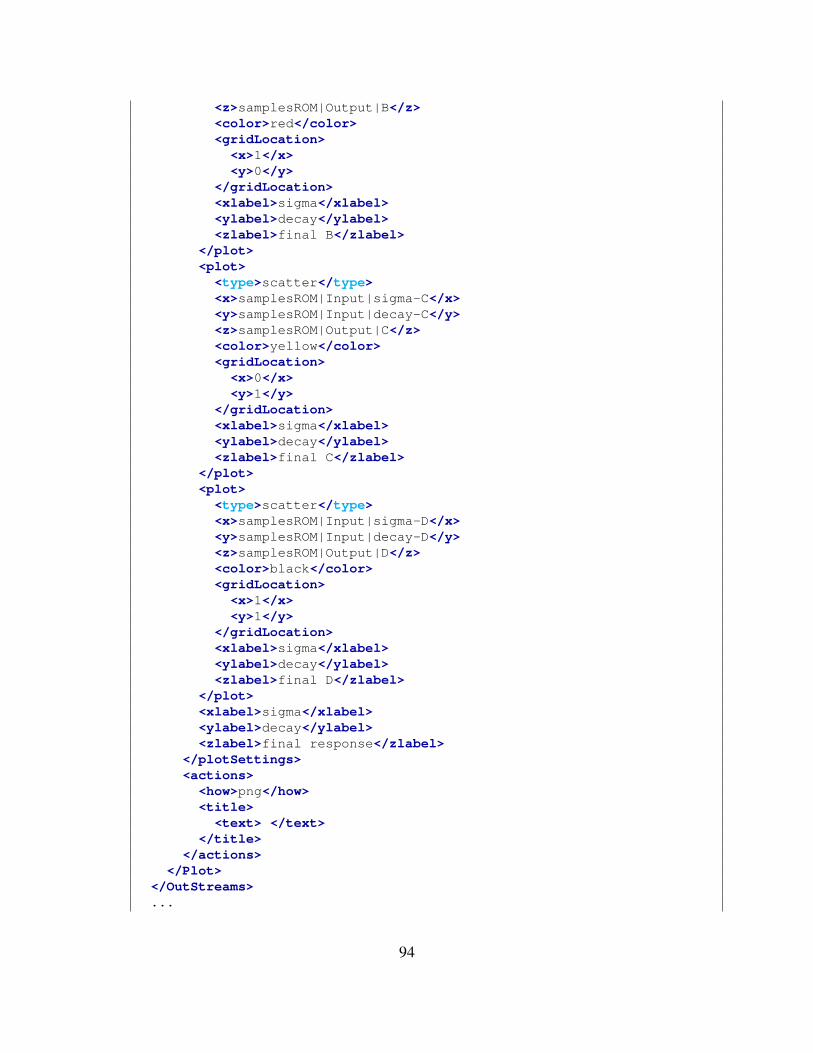
<z>samplesROM|Output|B</z><color>red</color><gridLocation>
<x>1</x><y>0</y>
</gridLocation><xlabel>sigma</xlabel><ylabel>decay</ylabel><zlabel>final B</zlabel>
</plot><plot>
<type>scatter</type><x>samplesROM|Input|sigma-C</x><y>samplesROM|Input|decay-C</y><z>samplesROM|Output|C</z><color>yellow</color><gridLocation>
<x>0</x><y>1</y>
</gridLocation><xlabel>sigma</xlabel><ylabel>decay</ylabel><zlabel>final C</zlabel>
</plot><plot>
<type>scatter</type><x>samplesROM|Input|sigma-D</x><y>samplesROM|Input|decay-D</y><z>samplesROM|Output|D</z><color>black</color><gridLocation>
<x>1</x><y>1</y>
</gridLocation><xlabel>sigma</xlabel><ylabel>decay</ylabel><zlabel>final D</zlabel>
</plot><xlabel>sigma</xlabel><ylabel>decay</ylabel><zlabel>final response</zlabel>
</plotSettings><actions>
<how>png</how><title>
<text> </text></title>
</actions></Plot>
</OutStreams>...
94
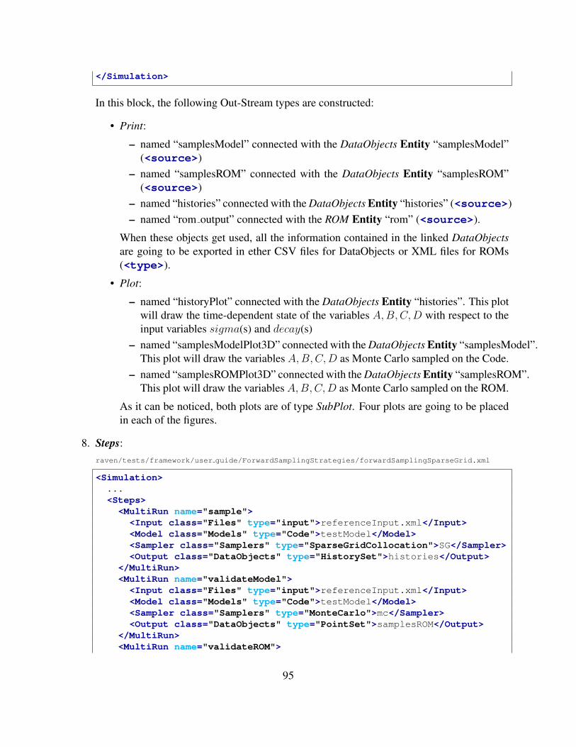
</Simulation>
In this block, the following Out-Stream types are constructed:
• Print:
– named “samplesModel” connected with the DataObjects Entity “samplesModel”(<source>)
– named “samplesROM” connected with the DataObjects Entity “samplesROM”(<source>)
– named “histories” connected with the DataObjects Entity “histories” (<source>)– named “rom output” connected with the ROM Entity “rom” (<source>).
When these objects get used, all the information contained in the linked DataObjectsare going to be exported in ether CSV files for DataObjects or XML files for ROMs(<type>).
• Plot:
– named “historyPlot” connected with the DataObjects Entity “histories”. This plotwill draw the time-dependent state of the variables A,B,C,D with respect to theinput variables sigma(s) and decay(s)
– named “samplesModelPlot3D” connected with the DataObjects Entity “samplesModel”.This plot will draw the variables A,B,C,D as Monte Carlo sampled on the Code.
– named “samplesROMPlot3D” connected with the DataObjects Entity “samplesROM”.This plot will draw the variables A,B,C,D as Monte Carlo sampled on the ROM.
As it can be noticed, both plots are of type SubPlot. Four plots are going to be placedin each of the figures.
8. Steps:raven/tests/framework/user guide/ForwardSamplingStrategies/forwardSamplingSparseGrid.xml
<Simulation>...<Steps>
<MultiRun name="sample"><Input class="Files" type="input">referenceInput.xml</Input><Model class="Models" type="Code">testModel</Model><Sampler class="Samplers" type="SparseGridCollocation">SG</Sampler><Output class="DataObjects" type="HistorySet">histories</Output>
</MultiRun><MultiRun name="validateModel"><Input class="Files" type="input">referenceInput.xml</Input><Model class="Models" type="Code">testModel</Model><Sampler class="Samplers" type="MonteCarlo">mc</Sampler><Output class="DataObjects" type="PointSet">samplesROM</Output>
</MultiRun><MultiRun name="validateROM">
95

<Input class="DataObjects" type="PointSet">inputPlaceholder</Input><Model class="Models" type="ROM">rom</Model><Sampler class="Samplers" type="MonteCarlo">mc</Sampler><Output class="DataObjects" type="PointSet">samplesModel</Output>
</MultiRun><IOStep name="output_print"><Input class="DataObjects" type="HistorySet">histories</Input><Input class="DataObjects" type="PointSet">samplesModel</Input><Input class="DataObjects" type="PointSet">samplesROM</Input><Input class="Models" type="ROM">rom</Input><Output class="OutStreams" type="Print">samplesModel</Output><Output class="OutStreams" type="Print">samplesROM</Output><Output class="OutStreams" type="Print">histories</Output><Output class="OutStreams" type="Print">rom_output</Output>
</IOStep><IOStep name="output_plot" pauseAtEnd="True"><Input class="DataObjects" type="HistorySet">histories</Input><Input class="DataObjects" type="PointSet">samplesModel</Input><Input class="DataObjects" type="PointSet">samplesROM</Input><Output class="OutStreams" type="Plot">historyPlot</Output><Output class="OutStreams" type="Plot">samplesModelPlot3D</Output><Output class="OutStreams" type="Plot">samplesROMPlot3D</Output>
</IOStep><RomTrainer name="train"><Input class="DataObjects" type="HistorySet">histories</Input><Output class="Models" type="ROM">rom</Output>
</RomTrainer></Steps>...
</Simulation>
Finally, the previously defined Entities can be combined in the <Steps> block. The fol-lowing <Steps> have been defined:
• <MultiRun> named “sample”, used to run the training samples of the driven code andcollect the outputs in the DataObjects. The <Sampler> is specified to communicateto the Step that the driven code needs to be sampled through the Sparse Grid Collocationsampling strategy;
• <RomTrainer> named “train”, used to train (i.e., construct) the GaussPolynomialROM. This step is essential if the user want to use the ROM in later steps;
• <MultiRun> named “sampleModel”, used to run the Monte Carlo perturbed samplesof the original Model for use in verification. The results are collected in the sam-plesModel DataObjects.
• <MultiRun> named “sampleROM”, used to run the Monte Carlo perturbed samplesof the previously constructed ROM for use in verificaiton. The results are collected inthe samplesROM DataObjects.
96
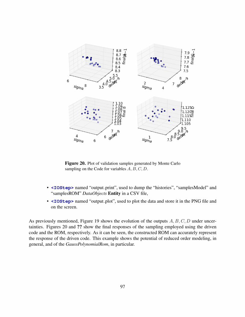
Figure 20. Plot of validation samples generated by Monte Carlosampling on the Code for variables A,B,C,D.
• <IOStep> named “output print”, used to dump the “histories”, “samplesModel” and“samplesROM” DataObjects Entity in a CSV file,
• <IOStep> named “output plot”, used to plot the data and store it in the PNG file andon the screen.
As previously mentioned, Figure 19 shows the evolution of the outputs A,B,C,D under uncer-tainties. Figures 20 and ?? show the final responses of the sampling employed using the drivencode and the ROM, respectively. As it can be seen, the constructed ROM can accurately representthe response of the driven code. This example shows the potential of reduced order modeling, ingeneral, and of the GaussPolynomialRom, in particular.
97

Figure 21. Plot of validation samples generated by Monte Carlosampling on the ROM for variables A,B,C,D.
98
4 Adaptive Sampling Strategies
Performing UQ and Dynamic PRA can be challenging from a computational point of view. TheForward sampling strategies reported in the previous Section can lead to a large number of unnec-essary evaluations of the physical model leading to an unacceptable resource expenses (CPU time).In addition, the Forward methodologies are not designed to leverage the information content thatis extractable from the simulations already concluded.
To overcome these limitations, in RAVEN several adaptive algorithms are available:
1. Limit Surface Search
2. Adaptive Dynamic Event Tree
3. Adaptive Hybrid Dynamic Event Tree
4. Adaptive Sparse Grid
5. Adaptive Sobol Decomposition.
In this Section, we will only show how to use the first algorithm.
4.1 Limit Surface Search sampling through RAVEN
The goal of this Section is to learn how to:
1. Set up a LS Search sampling for efficiently perturb a driven code
2. Use the LS Integral Post-processor for computing the probability of failure of the systemsubject to the same “goal” function
3. Plot the obtained LS.
In order to accomplish these tasks, the following RAVEN Entities (XML blocks in the input files)are defined:
1. RunInfo:
raven/tests/framework/user guide/AdaptiveSamplingStrategies/adaptiveSamplingLSsearch.xml
99

<Simulation>...<RunInfo><JobName>LSsearch</JobName><Sequence>sample,computeLSintegral,writeHistories</Sequence><WorkingDir>LSsearch</WorkingDir><batchSize>1</batchSize>
</RunInfo>...
</Simulation>
As shown in Section ??, the RunInfo Entity is intended to set up the analysis that the userwants to perform. In this specific case, three steps (<Sequence>) are sequentially runusing eight processors (<batchSize>).
2. Files:raven/tests/framework/user guide/AdaptiveSamplingStrategies/adaptiveSamplingLSsearch.xml
<Simulation>...<Files>
<Input name="referenceInput.xml"type="input">referenceInput.xml</Input>
<Input name="LSintegral.csv" type="">LSintegral.csv</Input></Files>...
</Simulation>
Since the driven code uses a single input file, in this Section the original input is placed. Asdetailed in the user manual the attribute name represents the alias that is going to be used inall the other input blocks in order to refer to this file.In addition the output file used in <Sequence> computeLSintegral is here inputted.
3. Models:raven/tests/framework/user guide/AdaptiveSamplingStrategies/adaptiveSamplingLSsearch.xml
<Simulation>...<Models><Code name="testModel" subType="GenericCode">
<executable>../physicalCode/analyticalbateman/AnalyticalDplMain.py</executable><clargs arg="python" type="prepend" /><clargs arg="" extension=".xml" type="input" /><clargs arg=" " extension=".csv" type="output" />
</Code><ROM name="AccelerationROM" subType="SciKitLearn">
<Features>sigma-A,decay-A</Features><Target>goalFunction</Target><SKLtype>neighbors|KNeighborsClassifier</SKLtype><algorithm>brute</algorithm><n_neighbors>1</n_neighbors>
100

</ROM><PostProcessor name="integralLS" subType="LimitSurfaceIntegral">
<tolerance>0.001</tolerance><integralType>MonteCarlo</integralType><seed>20021986</seed><target>goalFunction</target><variable name="sigma-A">
<distribution>sigmaA</distribution></variable><variable name="decay-A">
<distribution>decayConstantA</distribution></variable><outputName>EventProbability</outputName>
</PostProcessor></Models>...
</Simulation>
As mentioned above, the goal of this example is the employment of an efficient samplingstrategy, having as goal the determination of the failure of a system.
In addition to the previously explained Code model, the ROM of type SciKitLearn is herespecified. The ROM will be used in the adaptive sampling strategy LimitSurfaceSearch inorder to accelerate the convergence of the method. As it can be seen, a nearest neighborclassifier is used, targeting only two uncertainties sigma− Aanddecay − A.For the computation of the probability of failure (see the following), a Post-Processor (PP) oftype LimitSurfaceIntegral is here specified.This PP performs an integral of the LS generatedby the adaptive sampling technique.
4. Distributions:
raven/tests/framework/user guide/AdaptiveSamplingStrategies/adaptiveSamplingLSsearch.xml
<Simulation>...<Distributions>
<Uniform name="sigmaA"><lowerBound>0</lowerBound><upperBound>1000</upperBound>
</Uniform><Uniform name="decayConstantA">
<lowerBound>0.00000001</lowerBound><upperBound>0.0000001</upperBound>
</Uniform></Distributions>...
</Simulation>
In the Distributions XML Section, the stochastic model for the uncertainties treated by theLS search sampling are reported. In this case two distributions are defined:
101

• sigmaA ∼ U(0, 1000), used to model the uncertainty associated with the Modelsigma-A
• decayConstantA ∼ U(1e− 8, 1e− 7), used to model the uncertainty associated withthe Model decay-A.
5. Samplers:raven/tests/framework/user guide/AdaptiveSamplingStrategies/adaptiveSamplingLSsearch.xml
<Simulation>...<Samplers><LimitSurfaceSearch name="LSsearchSampler"><ROM class="Models" type="ROM">AccelerationROM</ROM><Function class="Functions" type="External">goalFunction</Function><TargetEvaluation class="DataObjects" type="PointSet">samples</TargetEvaluation><Convergence forceIteration="False" limit="50000" persistence="20" weight="CDF">0.00001</Convergence><variable name="sigma-A">
<distribution>sigmaA</distribution></variable><variable name="decay-A">
<distribution>decayConstantA</distribution></variable>
</LimitSurfaceSearch></Samplers>...
</Simulation>
In order to employ the LS search sampling strategy, a <LimitSurfaceSearch> nodeneeds to be inputted. As it can be seen from above, each variable is associated to a differentdistribution defined in the <Distributions> block. In addition, the AccelerationROM<ROM> is inputted. As already mentioned, this ROM (of type classifier) is used to acceleratethe convergence of the LS Search method. In addition, the goal function goalFunction andthe samples are here reported.For this example, a convergence criterion of 1.0e− 5 is set. To reach such a confidence witha Monte-Carlo, millions of samples would be needed.
6. Functions:
raven/tests/framework/user guide/AdaptiveSamplingStrategies/adaptiveSamplingLSsearch.xml
<Simulation>...<Functions>
<External file="goalFunction" name="goalFunction"><variable>A</variable>
</External></Functions>...
</Simulation>
As already mentioned, the LS search sampling strategy uses a goal function in order toidentify the regions of the uncertain space that are more informative. The goalFunction usedfor this example is reported below. As it can be seen, if the final response A is <= of 0.3 ,the system is considered to be in a “safe” condition.
102

def __residuumSign(self):returnValue = 1.0if self.A <= 0.3:
returnValue = -1.0return returnValue
7. DataObjects:
raven/tests/framework/user guide/AdaptiveSamplingStrategies/adaptiveSamplingLSsearch.xml
<Simulation>...<DataObjects>
<PointSet name="limitSurface"><Input>sigma-A,decay-A</Input><Output>goalFunction</Output>
</PointSet><PointSet name="limitSurfaceIntegral">
<Input>sigma-A,decay-A</Input><Output>goalFunction,EventProbability</Output>
</PointSet><PointSet name="samples">
<Input>sigma-A,decay-A</Input><Output>A,B,C,D,time</Output>
</PointSet><HistorySet name="histories">
<Input>sigma-A,decay-A</Input><Output>A,B,C,D,time</Output>
</HistorySet></DataObjects>...
</Simulation>
In this block, three DataObjects are defined: 1) PointSet named “samples” used to collect thefinal outcomes of the code, 2) HistorySet named “histories” in which the full time responsesof the variables A,B,C,D are going to be stored, 3) PointSet named “limitSurface” usedto export the LS location (in the uncertain space) during the employment of the samplingstrategy.
8. OutStreams:raven/tests/framework/user guide/AdaptiveSamplingStrategies/adaptiveSamplingLSsearch.xml
<Simulation>...
103
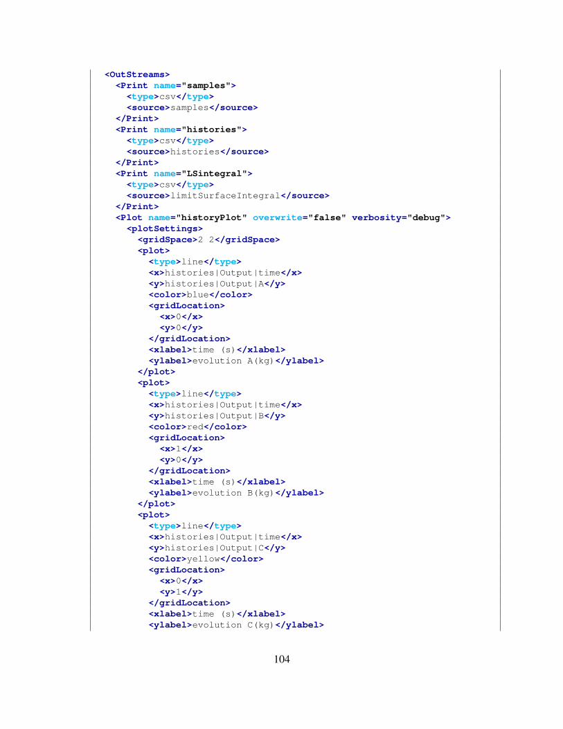
<OutStreams><Print name="samples"><type>csv</type><source>samples</source>
</Print><Print name="histories"><type>csv</type><source>histories</source>
</Print><Print name="LSintegral"><type>csv</type><source>limitSurfaceIntegral</source>
</Print><Plot name="historyPlot" overwrite="false" verbosity="debug"><plotSettings>
<gridSpace>2 2</gridSpace><plot>
<type>line</type><x>histories|Output|time</x><y>histories|Output|A</y><color>blue</color><gridLocation>
<x>0</x><y>0</y>
</gridLocation><xlabel>time (s)</xlabel><ylabel>evolution A(kg)</ylabel>
</plot><plot>
<type>line</type><x>histories|Output|time</x><y>histories|Output|B</y><color>red</color><gridLocation>
<x>1</x><y>0</y>
</gridLocation><xlabel>time (s)</xlabel><ylabel>evolution B(kg)</ylabel>
</plot><plot>
<type>line</type><x>histories|Output|time</x><y>histories|Output|C</y><color>yellow</color><gridLocation>
<x>0</x><y>1</y>
</gridLocation><xlabel>time (s)</xlabel><ylabel>evolution C(kg)</ylabel>
104
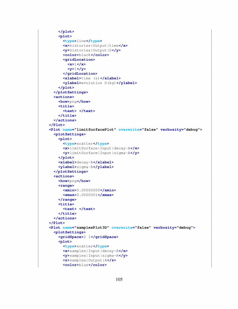
</plot><plot>
<type>line</type><x>histories|Output|time</x><y>histories|Output|D</y><color>black</color><gridLocation>
<x>1</x><y>1</y>
</gridLocation><xlabel>time (s)</xlabel><ylabel>evolution D(kg)</ylabel>
</plot></plotSettings><actions>
<how>png</how><title>
<text> </text></title>
</actions></Plot><Plot name="limitSurfacePlot" overwrite="false" verbosity="debug"><plotSettings>
<plot><type>scatter</type><x>limitSurface|Input|decay-A</x><y>limitSurface|Input|sigma-A</y>
</plot><xlabel>decay-A</xlabel><ylabel>sigma-A</ylabel>
</plotSettings><actions>
<how>png</how><range>
<xmin>0.00000000</xmin><xmax>0.0000001</xmax>
</range><title>
<text> </text></title>
</actions></Plot><Plot name="samplesPlot3D" overwrite="false" verbosity="debug"><plotSettings>
<gridSpace>2 1</gridSpace><plot>
<type>scatter</type><x>samples|Input|decay-A</x><y>samples|Input|sigma-A</y><z>samples|Output|A</z><color>blue</color>
105

<gridLocation><x>0</x><y>0</y>
</gridLocation><xlabel>decay-A</xlabel><ylabel>sigma-A</ylabel><zlabel>final A</zlabel>
</plot><plot>
<type>scatter</type><x>samples|Input|decay-A</x><y>samples|Input|sigma-A</y><z>samples|Output|B</z><color>blue</color><gridLocation>
<x>1</x><y>0</y>
</gridLocation><xlabel>decay-A</xlabel><ylabel>sigma-A</ylabel><zlabel>final B</zlabel>
</plot><xlabel>decay</xlabel><ylabel>sigma</ylabel><zlabel>final response</zlabel>
</plotSettings><actions>
<how>png</how><title>
<text> </text></title>
</actions></Plot>
</OutStreams>...
</Simulation>
Several out streams are included in this workflow, two for printing and three for plotting:
• “samples”, which writes the validation sample contents of the ’samples’ PointSetDataObject to a CSV file,
• “histories”, which writes the sampling contents of the ’histories’ HistorySetDataObject to a set of connected CSV files,
• “historyPlot”, which plots the evolution of the samples taken,
• “limitSurfacePlot”, which plots the limit surface discovered by the PostProcessor,
• “samplesPlot3D”, which plots the final state of the samples taken against the figures ofmerit.
106
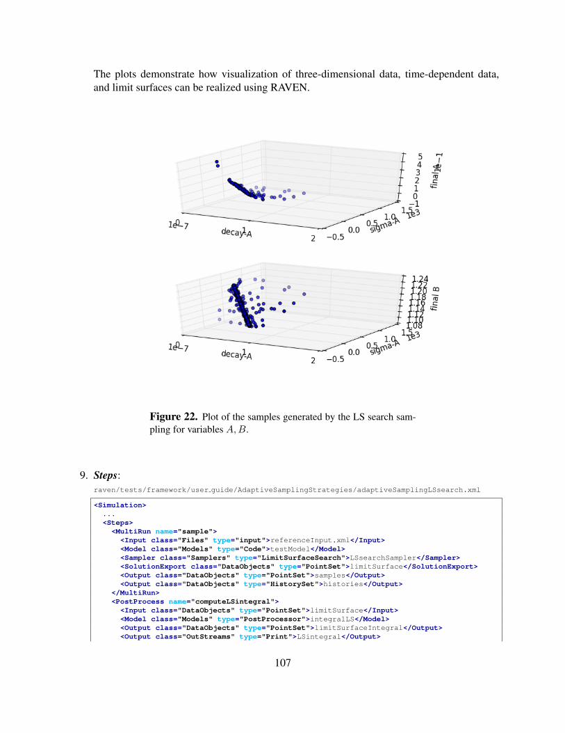
The plots demonstrate how visualization of three-dimensional data, time-dependent data,and limit surfaces can be realized using RAVEN.
Figure 22. Plot of the samples generated by the LS search sam-pling for variables A,B.
9. Steps:raven/tests/framework/user guide/AdaptiveSamplingStrategies/adaptiveSamplingLSsearch.xml
<Simulation>...<Steps><MultiRun name="sample">
<Input class="Files" type="input">referenceInput.xml</Input><Model class="Models" type="Code">testModel</Model><Sampler class="Samplers" type="LimitSurfaceSearch">LSsearchSampler</Sampler><SolutionExport class="DataObjects" type="PointSet">limitSurface</SolutionExport><Output class="DataObjects" type="PointSet">samples</Output><Output class="DataObjects" type="HistorySet">histories</Output>
</MultiRun><PostProcess name="computeLSintegral">
<Input class="DataObjects" type="PointSet">limitSurface</Input><Model class="Models" type="PostProcessor">integralLS</Model><Output class="DataObjects" type="PointSet">limitSurfaceIntegral</Output><Output class="OutStreams" type="Print">LSintegral</Output>
107
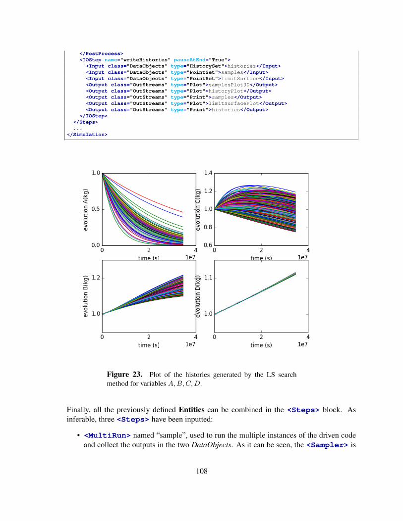
</PostProcess><IOStep name="writeHistories" pauseAtEnd="True">
<Input class="DataObjects" type="HistorySet">histories</Input><Input class="DataObjects" type="PointSet">samples</Input><Input class="DataObjects" type="PointSet">limitSurface</Input><Output class="OutStreams" type="Plot">samplesPlot3D</Output><Output class="OutStreams" type="Plot">historyPlot</Output><Output class="OutStreams" type="Print">samples</Output><Output class="OutStreams" type="Plot">limitSurfacePlot</Output><Output class="OutStreams" type="Print">histories</Output>
</IOStep></Steps>...
</Simulation>
Figure 23. Plot of the histories generated by the LS searchmethod for variables A,B,C,D.
Finally, all the previously defined Entities can be combined in the <Steps> block. Asinferable, three <Steps> have been inputted:
• <MultiRun> named “sample”, used to run the multiple instances of the driven codeand collect the outputs in the two DataObjects. As it can be seen, the <Sampler> is
108
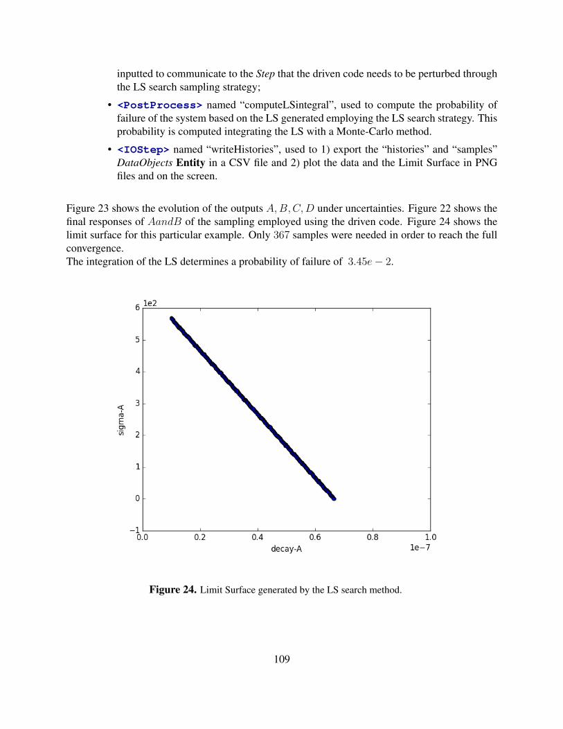
inputted to communicate to the Step that the driven code needs to be perturbed throughthe LS search sampling strategy;
• <PostProcess> named “computeLSintegral”, used to compute the probability offailure of the system based on the LS generated employing the LS search strategy. Thisprobability is computed integrating the LS with a Monte-Carlo method.
• <IOStep> named “writeHistories”, used to 1) export the “histories” and “samples”DataObjects Entity in a CSV file and 2) plot the data and the Limit Surface in PNGfiles and on the screen.
Figure 23 shows the evolution of the outputs A,B,C,D under uncertainties. Figure 22 shows thefinal responses of AandB of the sampling employed using the driven code. Figure 24 shows thelimit surface for this particular example. Only 367 samples were needed in order to reach the fullconvergence.The integration of the LS determines a probability of failure of 3.45e− 2.
Figure 24. Limit Surface generated by the LS search method.
109

5 Sampling from Restart
In some instances, there are existing solutions stored that are useful to a new sampling calculation.For example, if a Monte Carlo run collects 1000 runs, then later the user decides to expand to 1500runs, the original 1000 should not be wasted. In this case, it is desirable to restart sampling.
All <Sampler> entities in RAVEN accept the <Restart> node, which allows the user toprovide a <DataObject> from which sampling can draw. The way each sampler interacts withthis restart data is dependent on the sampling strategy.
Random sampling strategies, such as the <MonteCarlo> and <Stratified> samplers,increment the random number generator by the number of samples in the restart data, then continuesampling as normal.
Grid-based sampling strategies, such as <Grid>, <SparseGridCollocation>, and <Sobol>,require specific sampling points. As each required point in the input space is determined, the sam-pler will check the restart data for a match. If a match is found, the corresponding output values areused instead of sampling the <Model> for that point in the input space. In order to determine amatch, all of the values in the restart point must be within a relative tolerance of the correspondingpoint required by the sampler. While RAVEN has a default tolerance of 1e-15, the user can adjustthis tolerance using the <restartNode> node in the <Sampler> block.
In order to demonstrate this restart method, we include here an example of restarting a <Grid>sampler. This example runs a simple example Python code from the command line using the<GenericCode> interface. Within the run the following steps occur:
1. A grid is sampled that includes only the endpoints in each dimension.
2. The results of the first sampling are written to file.
3. The results in the CSV are read back in to a new <DataObject> called ’restart’.
4. A second, more dense grid is sampled that requires the points of the first sampling, plusseveral more. The results are added both to the original <DataObject> as well as a newone, for demonstration purposes.
5. The results of only the new sampling can be written to CSV because we added the seconddata object in the last step.
6. Lastly, the complete <DataObject> is written to file, including both the original and moredense sampling.
By looking at the contents of GRIDdump1.csv, GRIDdump2.csv, and GRIDdump3.csv,the progressive construction of the data object becomes clear. GRIDdump1.csv contains only
110
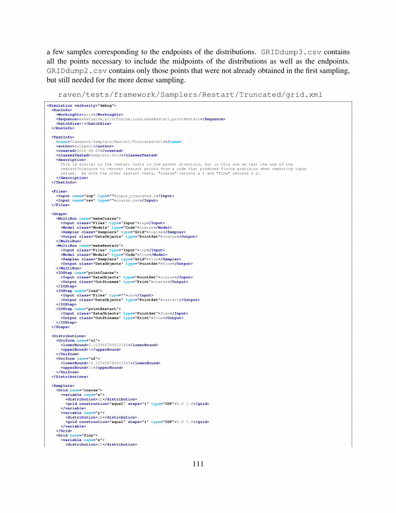
a few samples corresponding to the endpoints of the distributions. GRIDdump3.csv containsall the points necessary to include the midpoints of the distributions as well as the endpoints.GRIDdump2.csv contains only those points that were not already obtained in the first sampling,but still needed for the more dense sampling.
raven/tests/framework/Samplers/Restart/Truncated/grid.xml<Simulation verbosity="debug"><RunInfo>
<WorkingDir>grid</WorkingDir><Sequence>makeCoarse,printCoarse,load,makeRestart,printRestart</Sequence><batchSize>1</batchSize>
</RunInfo>
<TestInfo><name>framework/Samplers/Restart/Truncated/Grid</name><author>talbpaul</author><created>2016-04-05</created><classesTested>Samplers.Grid</classesTested><description>
This is similar to the restart tests in the parent directory, but in this one we test the use of therestartTolerance to recover restart points from a code that produces finite precision when reporting inputvalues. As with the other restart tests, "coarse" returns a 1 and "fine" returns a 2.
</description></TestInfo>
<Files><Input name="inp" type="">input_truncated.i</Input><Input name="csv" type="">coarse.csv</Input>
</Files>
<Steps><MultiRun name="makeCoarse">
<Input class="Files" type="Input">inp</Input><Model class="Models" type="Code">coarse</Model><Sampler class="Samplers" type="Grid">coarse</Sampler><Output class="DataObjects" type="PointSet">coarse</Output>
</MultiRun><MultiRun name="makeRestart">
<Input class="Files" type="Input">inp</Input><Model class="Models" type="Code">fine</Model><Sampler class="Samplers" type="Grid">fine</Sampler><Output class="DataObjects" type="PointSet">fine</Output>
</MultiRun><IOStep name="printCoarse">
<Input class="DataObjects" type="PointSet">coarse</Input><Output class="OutStreams" type="Print">coarse</Output>
</IOStep><IOStep name="load">
<Input class="Files" type="">csv</Input><Output class="DataObjects" type="PointSet">restart</Output>
</IOStep><IOStep name="printRestart">
<Input class="DataObjects" type="PointSet">fine</Input><Output class="OutStreams" type="Print">fine</Output>
</IOStep></Steps>
<Distributions><Uniform name="u1">
<lowerBound>0.123456789012345</lowerBound><upperBound>1</upperBound>
</Uniform><Uniform name="u2">
<lowerBound>10.123456789012345</lowerBound><upperBound>11</upperBound>
</Uniform></Distributions>
<Samplers><Grid name="coarse">
<variable name="x"><distribution>u1</distribution><grid construction="equal" steps="1" type="CDF">0.0 1.0</grid>
</variable><variable name="y">
<distribution>u2</distribution><grid construction="equal" steps="1" type="CDF">0.0 1.0</grid>
</variable></Grid><Grid name="fine">
<variable name="x"><distribution>u1</distribution>
111
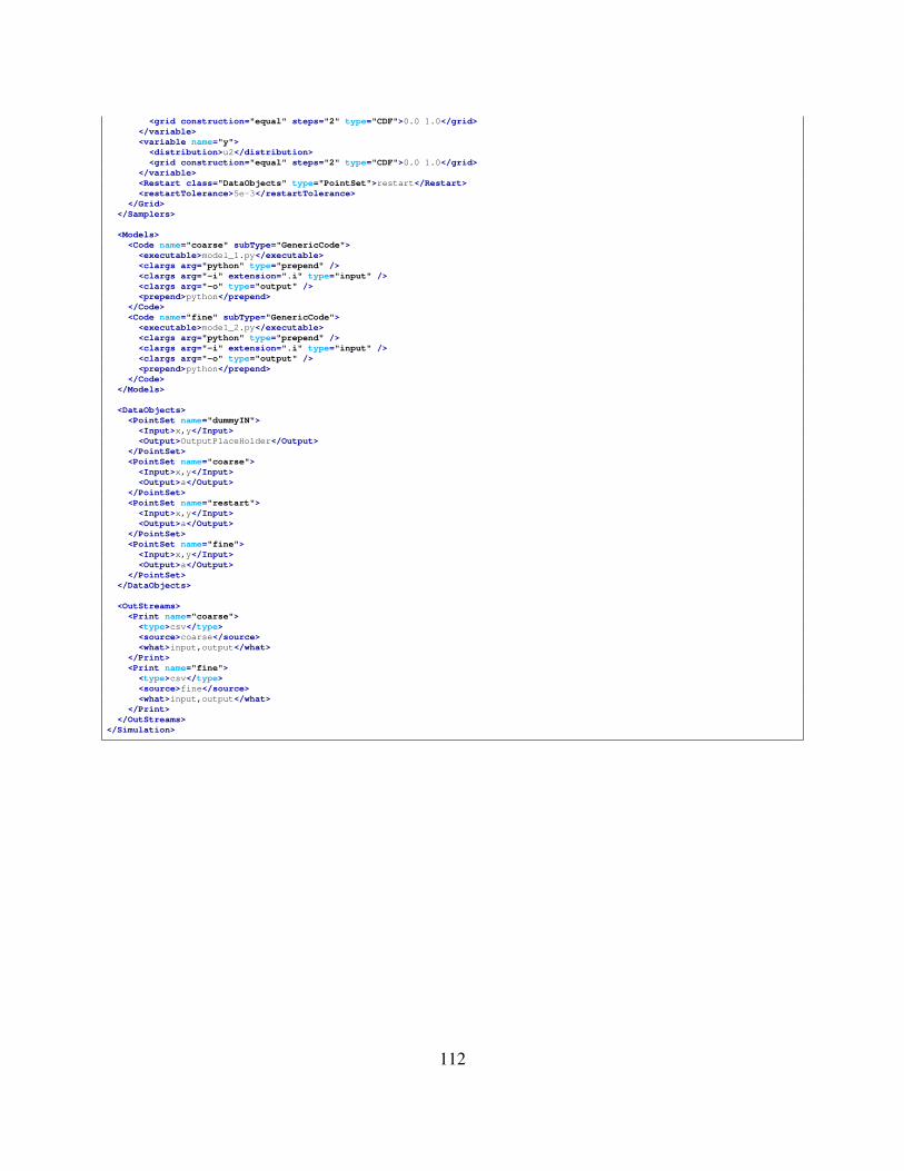
<grid construction="equal" steps="2" type="CDF">0.0 1.0</grid></variable><variable name="y">
<distribution>u2</distribution><grid construction="equal" steps="2" type="CDF">0.0 1.0</grid>
</variable><Restart class="DataObjects" type="PointSet">restart</Restart><restartTolerance>5e-3</restartTolerance>
</Grid></Samplers>
<Models><Code name="coarse" subType="GenericCode">
<executable>model_1.py</executable><clargs arg="python" type="prepend" /><clargs arg="-i" extension=".i" type="input" /><clargs arg="-o" type="output" /><prepend>python</prepend>
</Code><Code name="fine" subType="GenericCode">
<executable>model_2.py</executable><clargs arg="python" type="prepend" /><clargs arg="-i" extension=".i" type="input" /><clargs arg="-o" type="output" /><prepend>python</prepend>
</Code></Models>
<DataObjects><PointSet name="dummyIN">
<Input>x,y</Input><Output>OutputPlaceHolder</Output>
</PointSet><PointSet name="coarse">
<Input>x,y</Input><Output>a</Output>
</PointSet><PointSet name="restart">
<Input>x,y</Input><Output>a</Output>
</PointSet><PointSet name="fine">
<Input>x,y</Input><Output>a</Output>
</PointSet></DataObjects>
<OutStreams><Print name="coarse">
<type>csv</type><source>coarse</source><what>input,output</what>
</Print><Print name="fine">
<type>csv</type><source>fine</source><what>input,output</what>
</Print></OutStreams>
</Simulation>
112
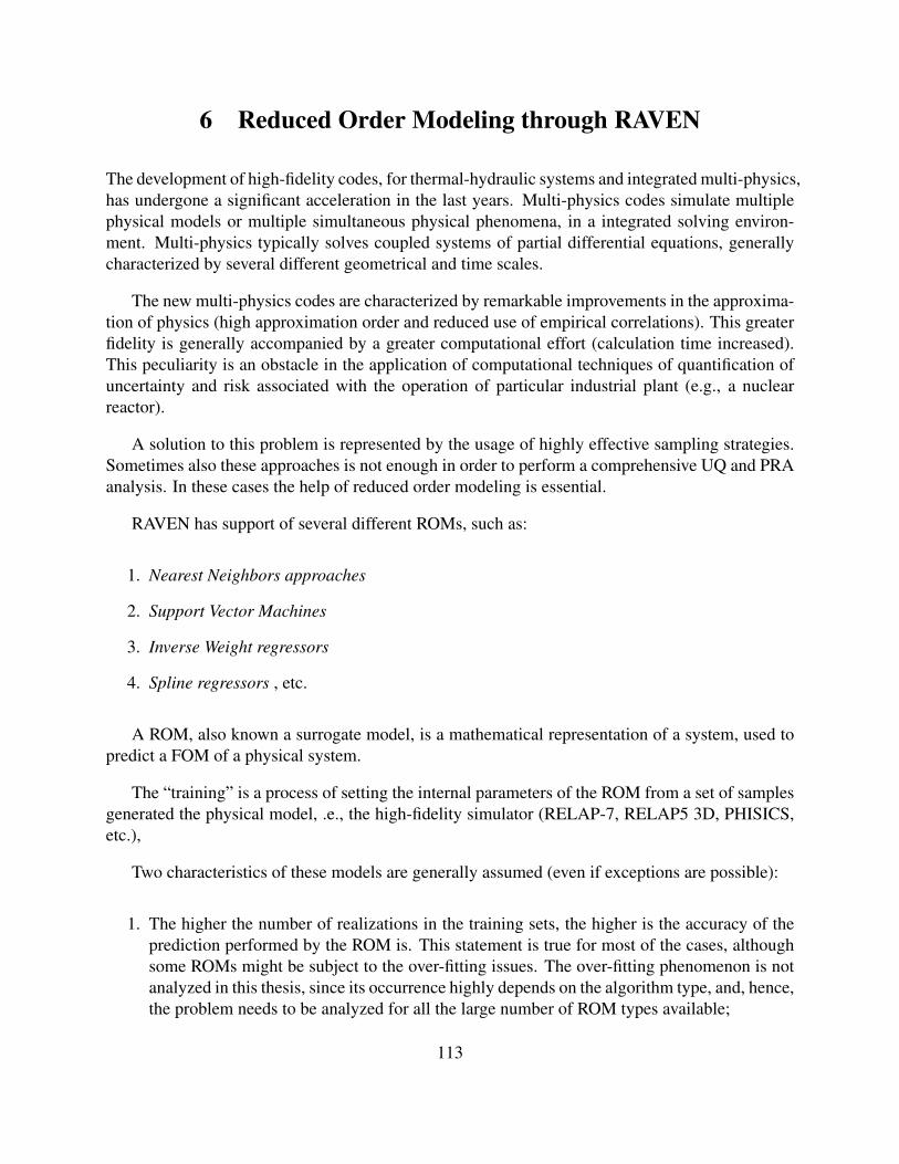
6 Reduced Order Modeling through RAVEN
The development of high-fidelity codes, for thermal-hydraulic systems and integrated multi-physics,has undergone a significant acceleration in the last years. Multi-physics codes simulate multiplephysical models or multiple simultaneous physical phenomena, in a integrated solving environ-ment. Multi-physics typically solves coupled systems of partial differential equations, generallycharacterized by several different geometrical and time scales.
The new multi-physics codes are characterized by remarkable improvements in the approxima-tion of physics (high approximation order and reduced use of empirical correlations). This greaterfidelity is generally accompanied by a greater computational effort (calculation time increased).This peculiarity is an obstacle in the application of computational techniques of quantification ofuncertainty and risk associated with the operation of particular industrial plant (e.g., a nuclearreactor).
A solution to this problem is represented by the usage of highly effective sampling strategies.Sometimes also these approaches is not enough in order to perform a comprehensive UQ and PRAanalysis. In these cases the help of reduced order modeling is essential.
RAVEN has support of several different ROMs, such as:
1. Nearest Neighbors approaches
2. Support Vector Machines
3. Inverse Weight regressors
4. Spline regressors , etc.
A ROM, also known a surrogate model, is a mathematical representation of a system, used topredict a FOM of a physical system.
The “training” is a process of setting the internal parameters of the ROM from a set of samplesgenerated the physical model, .e., the high-fidelity simulator (RELAP-7, RELAP5 3D, PHISICS,etc.),
Two characteristics of these models are generally assumed (even if exceptions are possible):
1. The higher the number of realizations in the training sets, the higher is the accuracy of theprediction performed by the ROM is. This statement is true for most of the cases, althoughsome ROMs might be subject to the over-fitting issues. The over-fitting phenomenon is notanalyzed in this thesis, since its occurrence highly depends on the algorithm type, and, hence,the problem needs to be analyzed for all the large number of ROM types available;
113

Figure 25. Example of reduced order model representation ofphysical system (regression).
2. The smaller the size of the input (uncertain) domain with respect to the variability of thesystem response, the more likely the ROM is able to represent the system response space.
The goals of this section are about learning how to:
1. Set up a sampling strategy to construct multiple ROMs, perturbing a driven code
2. Train the different ROMs with the data-set obtained by the applied sampling strategy;
3. Use the same sampling strategy, perturbing the ROMs
4. Plot the responses of the driven code and ROMs, respectively.
In order to accomplish these tasks, the following RAVEN Entities (XML blocks in the input files)need to be defined:
1. RunInfo:
raven/tests/framework/user guide/ReducedOrderModeling/reducedOrderModeling.xml
114

<Simulation>...<RunInfo>
<JobName>ROMConstruction</JobName><Sequence>
sample,trainROMGaussianProcess,trainROMsvm,trainROMinverse,sampleROMGaussianProcess,sampleROMInverse,sampleROMsvm,writeHistories
</Sequence><WorkingDir>ROMConstruction</WorkingDir><batchSize>8</batchSize>
</RunInfo>...
</Simulation>
As in the other examples, the the RunInfo Entity is intended to set up the analysis sequencethat needs to be performed. In this specific case, eight steps (<Sequence>) are going to besequentially run using eight processors (<batchSize>).In the first step, the original physical model is going to be sampled. The obtained resultsare going to be used to train three different ROMs.These ROMs are sampled by the samestrategy used in the first step in order to compare the ROMs’ responses with the ones comingfrom the original physical model.
2. Files:raven/tests/framework/user guide/ReducedOrderModeling/reducedOrderModeling.xml
<Simulation>...<Files>
<Input name="referenceInput.xml"type="input">referenceInput.xml</Input>
</Files>...
</Simulation>
Since the driven code uses a single input file, the original input is placed in this section. Asdetailed in the user manual the attribute name represents the alias that is going to be used inall the other input blocks in order to refer to this file.
3. Models:raven/tests/framework/user guide/ReducedOrderModeling/reducedOrderModeling.xml
<Simulation>...<Models><Code name="testModel" subType="GenericCode">
<executable>../physicalCode/analyticalbateman/AnalyticalDplMain.py</executable>
115
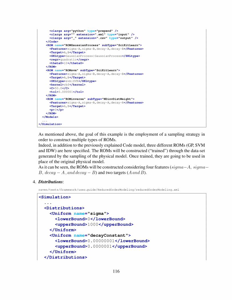
<clargs arg="python" type="prepend" /><clargs arg="" extension=".xml" type="input" /><clargs arg=" " extension=".csv" type="output" />
</Code><ROM name="ROMGaussianProcess" subType="SciKitLearn">
<Features>sigma-A,sigma-B,decay-A,decay-B</Features><Target>A,B</Target><SKLtype>GaussianProcess|GaussianProcess</SKLtype><regr>quadratic</regr><theta0>10</theta0>
</ROM><ROM name="ROMsvm" subType="SciKitLearn">
<Features>sigma-A,sigma-B,decay-A,decay-B</Features><Target>A,B</Target><SKLtype>svm|SVR</SKLtype><kernel>rbf</kernel><C>50.0</C><tol>0.000001</tol>
</ROM><ROM name="ROMinverse" subType="NDinvDistWeight">
<Features>sigma-A,sigma-B,decay-A,decay-B</Features><Target>A,B</Target><p>3</p>
</ROM></Models>...
</Simulation>
As mentioned above, the goal of this example is the employment of a sampling strategy inorder to construct multiple types of ROMs.Indeed, in addition to the previously explained Code model, three different ROMs (GP, SVMand IDW) are here specified. The ROMs will be constructed (“trained”) through the data-setgenerated by the sampling of the physical model. Once trained, they are going to be used inplace of the original physical model.As it can be seen, the ROMs will be constructed considering four features (sigma−A, sigma−B, decay − A , and decay −B) and two targets (AandB).
4. Distributions:
raven/tests/framework/user guide/ReducedOrderModeling/reducedOrderModeling.xml
<Simulation>...<Distributions>
<Uniform name="sigma"><lowerBound>0</lowerBound><upperBound>1000</upperBound>
</Uniform><Uniform name="decayConstant">
<lowerBound>0.00000001</lowerBound><upperBound>0.0000001</upperBound>
</Uniform></Distributions>
116
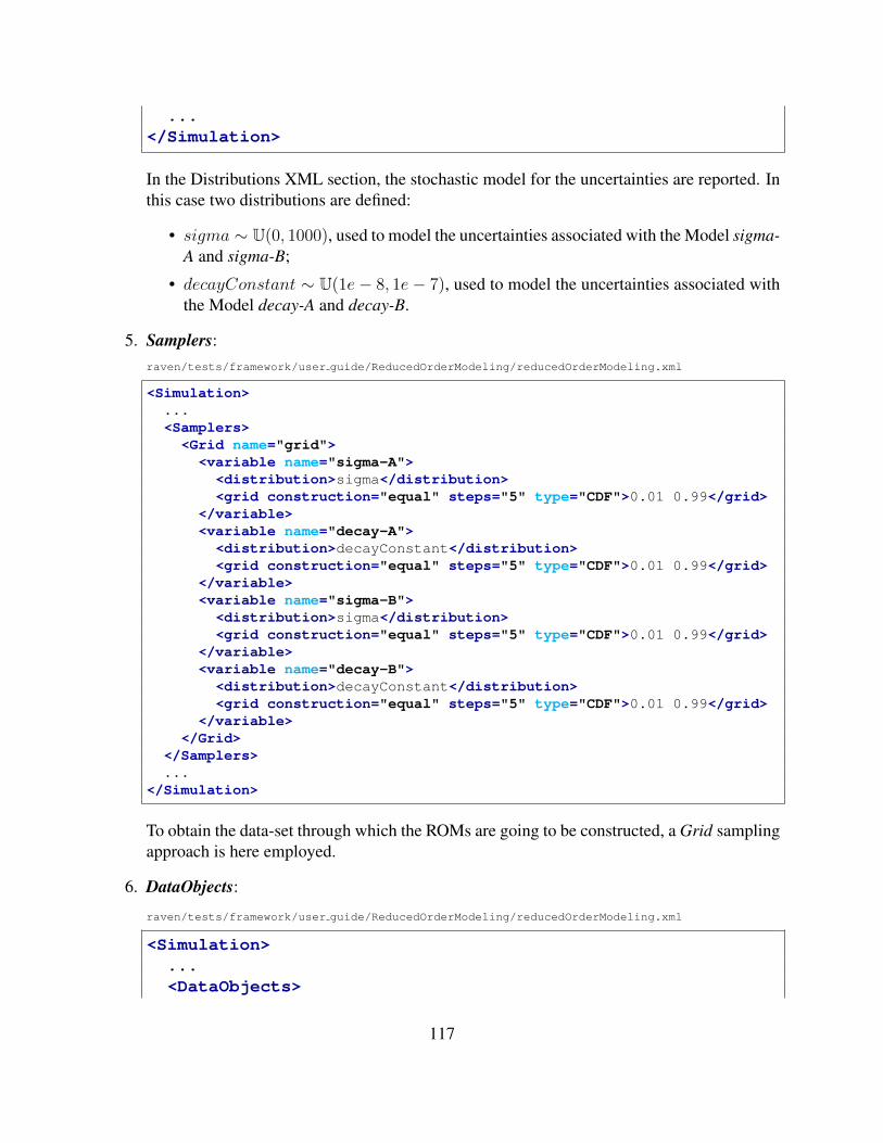
...</Simulation>
In the Distributions XML section, the stochastic model for the uncertainties are reported. Inthis case two distributions are defined:
• sigma ∼ U(0, 1000), used to model the uncertainties associated with the Model sigma-A and sigma-B;
• decayConstant ∼ U(1e− 8, 1e− 7), used to model the uncertainties associated withthe Model decay-A and decay-B.
5. Samplers:raven/tests/framework/user guide/ReducedOrderModeling/reducedOrderModeling.xml
<Simulation>...<Samplers>
<Grid name="grid"><variable name="sigma-A">
<distribution>sigma</distribution><grid construction="equal" steps="5" type="CDF">0.01 0.99</grid>
</variable><variable name="decay-A">
<distribution>decayConstant</distribution><grid construction="equal" steps="5" type="CDF">0.01 0.99</grid>
</variable><variable name="sigma-B">
<distribution>sigma</distribution><grid construction="equal" steps="5" type="CDF">0.01 0.99</grid>
</variable><variable name="decay-B">
<distribution>decayConstant</distribution><grid construction="equal" steps="5" type="CDF">0.01 0.99</grid>
</variable></Grid>
</Samplers>...
</Simulation>
To obtain the data-set through which the ROMs are going to be constructed, a Grid samplingapproach is here employed.
6. DataObjects:
raven/tests/framework/user guide/ReducedOrderModeling/reducedOrderModeling.xml
<Simulation>...<DataObjects>
117

<PointSet name="inputPlaceHolder"><Input>sigma-A,sigma-B,decay-A,decay-B</Input><Output>OutputPlaceHolder</Output>
</PointSet><PointSet name="samples">
<Input>sigma-A,sigma-B,decay-A,decay-B</Input><Output>A,B,C,D</Output>
</PointSet><PointSet name="samplesGP">
<Input>sigma-A,sigma-B,decay-A,decay-B</Input><Output>A,B</Output>
</PointSet><PointSet name="samplesInverse">
<Input>sigma-A,sigma-B,decay-A,decay-B</Input><Output>A,B</Output>
</PointSet><PointSet name="samplesSVM">
<Input>sigma-A,sigma-B,decay-A,decay-B</Input><Output>A,B</Output>
</PointSet><HistorySet name="histories">
<Input>sigma-A,sigma-B,decay-A,decay-B</Input><Output>A,B,C,D,time</Output>
</HistorySet></DataObjects>...
</Simulation>
Int this block, six DataObjects are defined: 1) PointSet named “samples” used to collect thefinal outcomes of the code, 2) HistorySet named “histories” in which the full time responsesof the variables A,B,C,D are going to be stored, 3) PointSet named “inputPlaceHolder”used in the role of <Input> for the ROMs sampling; 4) PointSet named “samplesGP” usedto collect the final outcomes (sampling) of the GP ROM; 5) PointSet named “samplesIn-verse” used to collect the final outcomes (sampling) of the IDW ROM; 6) PointSet named“samplesSVM” used to collect the final outcomes (sampling) of the SVM ROM.
7. OutStreams:
118
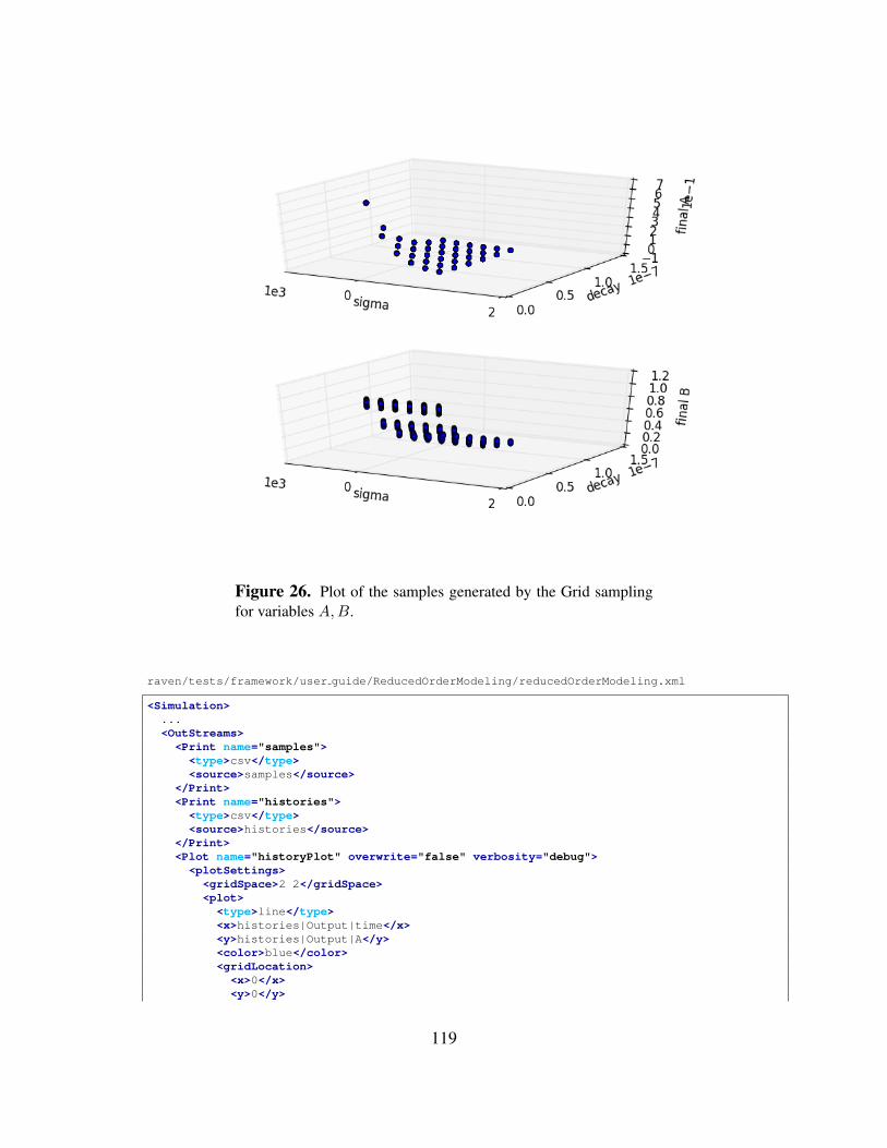
Figure 26. Plot of the samples generated by the Grid samplingfor variables A,B.
raven/tests/framework/user guide/ReducedOrderModeling/reducedOrderModeling.xml
<Simulation>...<OutStreams><Print name="samples">
<type>csv</type><source>samples</source>
</Print><Print name="histories">
<type>csv</type><source>histories</source>
</Print><Plot name="historyPlot" overwrite="false" verbosity="debug">
<plotSettings><gridSpace>2 2</gridSpace><plot><type>line</type><x>histories|Output|time</x><y>histories|Output|A</y><color>blue</color><gridLocation><x>0</x><y>0</y>
119
</gridLocation><xlabel>time (s)</xlabel><ylabel>evolution A(kg)</ylabel>
</plot><plot><type>line</type><x>histories|Output|time</x><y>histories|Output|B</y><color>red</color><gridLocation><x>1</x><y>0</y>
</gridLocation><xlabel>time (s)</xlabel><ylabel>evolution B(kg)</ylabel>
</plot><plot><type>line</type><x>histories|Output|time</x><y>histories|Output|C</y><color>yellow</color><gridLocation><x>0</x><y>1</y>
</gridLocation><xlabel>time (s)</xlabel><ylabel>evolution C(kg)</ylabel>
</plot><plot><type>line</type><x>histories|Output|time</x><y>histories|Output|D</y><color>black</color><gridLocation><x>1</x><y>1</y>
</gridLocation><xlabel>time (s)</xlabel><ylabel>evolution D(kg)</ylabel>
</plot></plotSettings><actions>
<how>png</how><title><text> </text>
</title></actions>
</Plot><Plot name="samplesPlot3D" overwrite="false" verbosity="debug">
<plotSettings><gridSpace>2 1</gridSpace><plot><type>scatter</type><x>samples|Input|sigma-A</x><y>samples|Input|decay-A</y><z>samples|Output|A</z><color>blue</color><gridLocation><x>0</x><y>0</y>
</gridLocation><xlabel>sigma</xlabel><ylabel>decay</ylabel><zlabel>final A</zlabel>
</plot>
120
<plot><type>scatter</type><x>samples|Input|sigma-B</x><y>samples|Input|decay-B</y><z>samples|Output|B</z><color>red</color><gridLocation><x>1</x><y>0</y>
</gridLocation><xlabel>sigma</xlabel><ylabel>decay</ylabel><zlabel>final B</zlabel>
</plot></plotSettings><actions>
<how>png</how><title><text> </text>
</title></actions>
</Plot><Plot name="samplesPlot3DROMgp" overwrite="false" verbosity="debug">
<plotSettings><gridSpace>2 1</gridSpace><plot><type>scatter</type><x>samplesGP|Input|sigma-A</x><y>samplesGP|Input|decay-A</y><z>samplesGP|Output|A</z><color>blue</color><gridLocation><x>0</x><y>0</y>
</gridLocation><xlabel>sigma</xlabel><ylabel>decay</ylabel><zlabel>final A</zlabel>
</plot><plot><type>scatter</type><x>samplesGP|Input|sigma-B</x><y>samplesGP|Input|decay-B</y><z>samplesGP|Output|B</z><color>red</color><gridLocation><x>1</x><y>0</y>
</gridLocation><xlabel>sigma</xlabel><ylabel>decay</ylabel><zlabel>final B</zlabel>
</plot></plotSettings><actions>
<how>png</how><title><text> </text>
</title></actions>
</Plot><Plot name="samplesPlot3DROMsvm" overwrite="false" verbosity="debug">
<plotSettings><gridSpace>2 1</gridSpace><plot>
121
<type>scatter</type><x>samplesSVM|Input|sigma-A</x><y>samplesSVM|Input|decay-A</y><z>samplesSVM|Output|A</z><color>blue</color><gridLocation><x>0</x><y>0</y>
</gridLocation><xlabel>sigma</xlabel><ylabel>decay</ylabel><zlabel>final A</zlabel>
</plot><plot><type>scatter</type><x>samplesSVM|Input|sigma-B</x><y>samplesSVM|Input|decay-B</y><z>samplesSVM|Output|B</z><color>red</color><gridLocation><x>1</x><y>0</y>
</gridLocation><xlabel>sigma</xlabel><ylabel>decay</ylabel><zlabel>final B</zlabel>
</plot></plotSettings><actions>
<how>png</how><title><text> </text>
</title></actions>
</Plot><Plot name="samplesPlot3DROMinverse" overwrite="false" verbosity="debug">
<plotSettings><gridSpace>2 1</gridSpace><plot><type>scatter</type><x>samplesInverse|Input|sigma-A</x><y>samplesInverse|Input|decay-A</y><z>samplesInverse|Output|A</z><color>blue</color><gridLocation><x>0</x><y>0</y>
</gridLocation><xlabel>sigma</xlabel><ylabel>decay</ylabel><zlabel>final A</zlabel>
</plot><plot><type>scatter</type><x>samplesInverse|Input|sigma-B</x><y>samplesInverse|Input|decay-B</y><z>samplesInverse|Output|B</z><color>red</color><gridLocation><x>1</x><y>0</y>
</gridLocation><xlabel>sigma</xlabel><ylabel>decay</ylabel><zlabel>final B</zlabel>
122
</plot></plotSettings><actions>
<how>png</how><title><text> </text>
</title></actions>
</Plot></OutStreams>...
</Simulation>
This model makes use of two Print OutStreams and five Plot OutStreams:
• “samples,” which writes the contents of the point-wise training samples to CSV,
• “histories,” which writes the contents of the history-wise training samples to linkedCSVs,
• “historyPlot,” which plots the evolution of the training samples,
• “samplesPlot3D,” which plots the final state of the training samples with relation to theoutputs of interest,
• “samplesPlot3DROMgp,” which plots the validation samples of the Gaussian ProcessROM,
• “samplesPlot3DROMsvm,” which plots the validation samples of the Support-VectorMachine ROM,
• “samplesPlot3Dinverse,” which plots the validation samples of the multidimensionalInverse Weight ROM.
The 3D plots of the samples as well as the ROM samples can be used as a view-norm vali-dation of the ROMs.
8. Steps:raven/tests/framework/user guide/ReducedOrderModeling/reducedOrderModeling.xml
<Simulation>...<Steps><MultiRun name="sample">
<Input class="Files" type="input">referenceInput.xml</Input><Model class="Models" type="Code">testModel</Model><Sampler class="Samplers" type="Grid">grid</Sampler><Output class="DataObjects" type="PointSet">samples</Output><Output class="DataObjects" type="HistorySet">histories</Output>
</MultiRun><MultiRun name="sampleROMGaussianProcess">
<Input class="DataObjects" type="PointSet">inputPlaceHolder</Input><Model class="Models" type="ROM">ROMGaussianProcess</Model><Sampler class="Samplers" type="Grid">grid</Sampler><Output class="DataObjects" type="PointSet">samplesGP</Output>
</MultiRun><MultiRun name="sampleROMInverse">
<Input class="DataObjects" type="PointSet">inputPlaceHolder</Input>
123
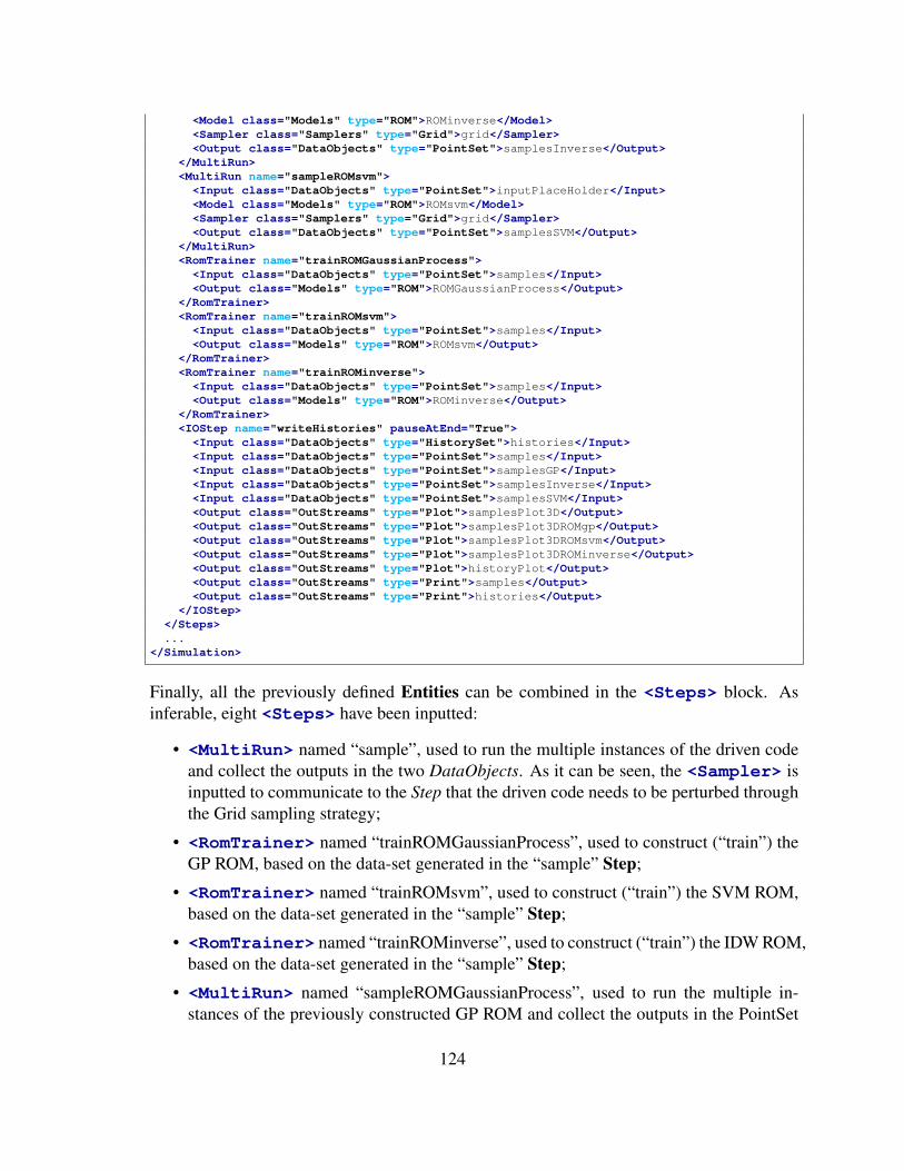
<Model class="Models" type="ROM">ROMinverse</Model><Sampler class="Samplers" type="Grid">grid</Sampler><Output class="DataObjects" type="PointSet">samplesInverse</Output>
</MultiRun><MultiRun name="sampleROMsvm">
<Input class="DataObjects" type="PointSet">inputPlaceHolder</Input><Model class="Models" type="ROM">ROMsvm</Model><Sampler class="Samplers" type="Grid">grid</Sampler><Output class="DataObjects" type="PointSet">samplesSVM</Output>
</MultiRun><RomTrainer name="trainROMGaussianProcess">
<Input class="DataObjects" type="PointSet">samples</Input><Output class="Models" type="ROM">ROMGaussianProcess</Output>
</RomTrainer><RomTrainer name="trainROMsvm">
<Input class="DataObjects" type="PointSet">samples</Input><Output class="Models" type="ROM">ROMsvm</Output>
</RomTrainer><RomTrainer name="trainROMinverse">
<Input class="DataObjects" type="PointSet">samples</Input><Output class="Models" type="ROM">ROMinverse</Output>
</RomTrainer><IOStep name="writeHistories" pauseAtEnd="True">
<Input class="DataObjects" type="HistorySet">histories</Input><Input class="DataObjects" type="PointSet">samples</Input><Input class="DataObjects" type="PointSet">samplesGP</Input><Input class="DataObjects" type="PointSet">samplesInverse</Input><Input class="DataObjects" type="PointSet">samplesSVM</Input><Output class="OutStreams" type="Plot">samplesPlot3D</Output><Output class="OutStreams" type="Plot">samplesPlot3DROMgp</Output><Output class="OutStreams" type="Plot">samplesPlot3DROMsvm</Output><Output class="OutStreams" type="Plot">samplesPlot3DROMinverse</Output><Output class="OutStreams" type="Plot">historyPlot</Output><Output class="OutStreams" type="Print">samples</Output><Output class="OutStreams" type="Print">histories</Output>
</IOStep></Steps>...
</Simulation>
Finally, all the previously defined Entities can be combined in the <Steps> block. Asinferable, eight <Steps> have been inputted:
• <MultiRun> named “sample”, used to run the multiple instances of the driven codeand collect the outputs in the two DataObjects. As it can be seen, the <Sampler> isinputted to communicate to the Step that the driven code needs to be perturbed throughthe Grid sampling strategy;
• <RomTrainer> named “trainROMGaussianProcess”, used to construct (“train”) theGP ROM, based on the data-set generated in the “sample” Step;
• <RomTrainer> named “trainROMsvm”, used to construct (“train”) the SVM ROM,based on the data-set generated in the “sample” Step;
• <RomTrainer> named “trainROMinverse”, used to construct (“train”) the IDW ROM,based on the data-set generated in the “sample” Step;
• <MultiRun> named “sampleROMGaussianProcess”, used to run the multiple in-stances of the previously constructed GP ROM and collect the outputs in the PointSet
124

Figure 27. Plot of the histories generated by the Grid method forvariables A,B,C,D.
DataObject. As it can be seen, the same <Sampler> used for perturbing the originalmodel is here used.
• <MultiRun> named “sampleROMsvm”, used to run the multiple instances of thepreviously constructed Support Vector Machine ROM and collect the outputs in thePointSet DataObject. As it can be seen, the same <Sampler> used for perturbing theoriginal model is here used.
• <MultiRun> named “sampleROMInverse”, used to run the multiple instances of thepreviously constructed Inverse Distance Weight ROM and collect the outputs in thePointSet DataObject. As it can be seen, the same <Sampler> used for perturbing theoriginal model is here used.
• <IOStep> named “writeHistories”, used to 1) export the “histories” and “samples”DataObjects Entity in a CSV file and 2) plot the responses of the sampling performedon the physical model, GP ROM, SVM ROM and IDW ROM in PNG files and on thescreen.
125

Figure 28. Plot of the samples generated by the Grid samplingapplied on the Gaussian Process ROM for variables A,B
Figure 27 shows the evolution of the outputs A,B,C,D under uncertainties. Figure 26 showsthe final responses of AandB of the sampling employed using the driven code.
Figures 28, 29 and 30 show the final responses of AandB of the sampling employed using theGaussian Process, Support Vector Machines and Inverse Distance Weight ROMs, respectively. Itcan be clearly noticed that the responses of the ROMs perfectly match the outcomes coming fromthe original model (see Figure 26).
126

Figure 29. Plot of the samples generated by the Grid samplingapplied on the Support Vector Machine ROM for variables A,B
127
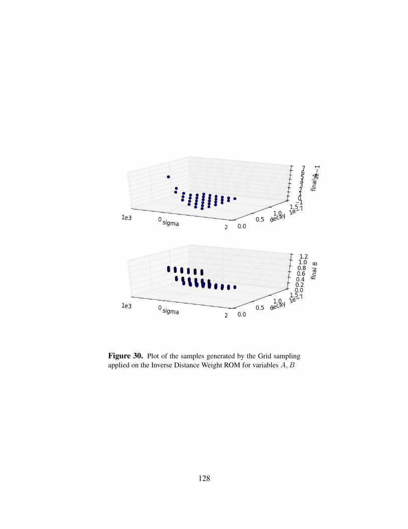
Figure 30. Plot of the samples generated by the Grid samplingapplied on the Inverse Distance Weight ROM for variables A,B
128

7 Statistical Analysis through RAVEN
In order to perform a complete analysis of a system under uncertainties, it is crucial to be able tocompute all the statistical moments of one or even multiple FOMs. In addition, it is essential toidentify the correlation among different FOMs toward a specific input space.
RAVEN is able to compute the most important statistical moments: such as:
1. Expected Value
2. Standard Deviation
3. Variance
4. variationCoefficient
5. Skewness
6. Kurtosis
7. Median
8. Percentile.
In addition, RAVEN fully supports the computation of all of the statistical moments defined to“measure” the correlation among variables/parameters/FOMs:
1. Covariance matrix
2. Normalized Sensitivity matrix
3. Variance Dependent Sensitivity matrix
4. Sensitivity matrix
5. Pearson matrix.
The goals of this section is to show how to:
1. Set up a sampling strategy to perform a final statistical analysis perturbing a driven code
2. Compute all the statistical moments and correlation/covariance metrics.
129
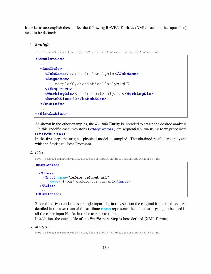
In order to accomplish these tasks, the following RAVEN Entities (XML blocks in the input files)need to be defined:
1. RunInfo:
raven/tests/framework/user guide/StatisticalAnalysis/statisticalAnalysis.xml
<Simulation>...<RunInfo>
<JobName>StatisticalAnalysis</JobName><Sequence>
sampleMC,statisticalAnalysisMC</Sequence><WorkingDir>StatisticalAnalysis</WorkingDir><batchSize>40</batchSize>
</RunInfo>...
</Simulation>
As shown in the other examples, the RunInfo Entity is intended to set up the desired analysis. In this specific case, two steps (<Sequence>) are sequentially run using forty processors(<batchSize>).In the first step, the original physical model is sampled. The obtained results are analyzedwith the Statistical Post-Processor.
2. Files:raven/tests/framework/user guide/StatisticalAnalysis/statisticalAnalysis.xml
<Simulation>...<Files>
<Input name="referenceInput.xml"type="input">referenceInput.xml</Input>
</Files>...
</Simulation>
Since the driven code uses a single input file, in this section the original input is placed. Asdetailed in the user manual the attribute name represents the alias that is going to be used inall the other input blocks in order to refer to this file.In addition, the output file of the PostProcess Step is here defined (XML format).
3. Models:raven/tests/framework/user guide/StatisticalAnalysis/statisticalAnalysis.xml
130
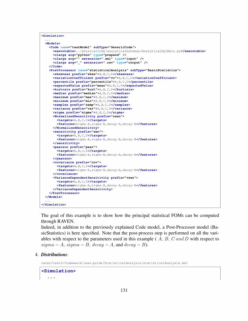
<Simulation>...<Models><Code name="testModel" subType="GenericCode">
<executable>../physicalCode/analyticalbateman/AnalyticalDplMain.py</executable><clargs arg="python" type="prepend" /><clargs arg="" extension=".xml" type="input" /><clargs arg=" " extension=".csv" type="output" />
</Code><PostProcessor name="statisticalAnalysis" subType="BasicStatistics">
<skewness prefix="skew">A,B,C,D</skewness><variationCoefficient prefix="vc">A,B,C,D</variationCoefficient><percentile prefix="percentile">A,B,C,D</percentile><expectedValue prefix="mean">A,B,C,D</expectedValue><kurtosis prefix="kurt">A,B,C,D</kurtosis><median prefix="median">A,B,C,D</median><maximum prefix="max">A,B,C,D</maximum><minimum prefix="min">A,B,C,D</minimum><samples prefix="samp">A,B,C,D</samples><variance prefix="var">A,B,C,D</variance><sigma prefix="sigma">A,B,C,D</sigma><NormalizedSensitivity prefix="nsen">
<targets>A,B,C,D</targets><features>sigma-A,sigma-B,decay-A,decay-B</features>
</NormalizedSensitivity><sensitivity prefix="sen">
<targets>A,B,C,D</targets><features>sigma-A,sigma-B,decay-A,decay-B</features>
</sensitivity><pearson prefix="pear">
<targets>A,B,C,D</targets><features>sigma-A,sigma-B,decay-A,decay-B</features>
</pearson><covariance prefix="cov">
<targets>A,B,C,D</targets><features>sigma-A,sigma-B,decay-A,decay-B</features>
</covariance><VarianceDependentSensitivity prefix="vsen">
<targets>A,B,C,D</targets><features>sigma-A,sigma-B,decay-A,decay-B</features>
</VarianceDependentSensitivity></PostProcessor>
</Models>...
</Simulation>
The goal of this example is to show how the principal statistical FOMs can be computedthrough RAVEN.Indeed, in addition to the previously explained Code model, a Post-Processor model (Ba-sicStatistics) is here specified. Note that the post-process step is performed on all the vari-ables with respect to the parameters used in this example ( A, B, C andD with respect tosigma− A, sigma−B, decay − A, and decay −B).
4. Distributions:
raven/tests/framework/user guide/StatisticalAnalysis/statisticalAnalysis.xml
<Simulation>...
131
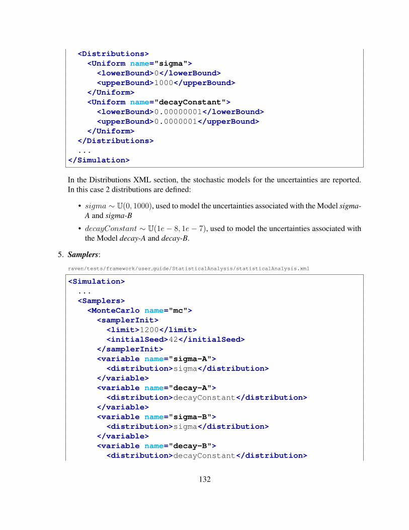
<Distributions><Uniform name="sigma">
<lowerBound>0</lowerBound><upperBound>1000</upperBound>
</Uniform><Uniform name="decayConstant">
<lowerBound>0.00000001</lowerBound><upperBound>0.0000001</upperBound>
</Uniform></Distributions>...
</Simulation>
In the Distributions XML section, the stochastic models for the uncertainties are reported.In this case 2 distributions are defined:
• sigma ∼ U(0, 1000), used to model the uncertainties associated with the Model sigma-A and sigma-B
• decayConstant ∼ U(1e− 8, 1e− 7), used to model the uncertainties associated withthe Model decay-A and decay-B.
5. Samplers:
raven/tests/framework/user guide/StatisticalAnalysis/statisticalAnalysis.xml
<Simulation>...<Samplers>
<MonteCarlo name="mc"><samplerInit><limit>1200</limit><initialSeed>42</initialSeed>
</samplerInit><variable name="sigma-A"><distribution>sigma</distribution>
</variable><variable name="decay-A"><distribution>decayConstant</distribution>
</variable><variable name="sigma-B"><distribution>sigma</distribution>
</variable><variable name="decay-B"><distribution>decayConstant</distribution>
132

</variable></MonteCarlo>
</Samplers>...
</Simulation>
In order to obtained the data-set through which the statistical FOMs need to be computed, aMonteCarlo sampling approach is here employed.
6. DataObjects:
raven/tests/framework/user guide/StatisticalAnalysis/statisticalAnalysis.xml
<Simulation>...<DataObjects>
<PointSet name="samplesMC"><Input>sigma-A,sigma-B,decay-A,decay-B</Input><Output>A,B,C,D</Output>
</PointSet><PointSet name="statisticalAnalysis_basicStatPP">
<Output>statisticalAnalysis_vars</Output></PointSet><HistorySet name="histories">
<Input>sigma-A,sigma-B,decay-A,decay-B</Input><Output>A,B,C,D,time</Output>
</HistorySet></DataObjects>...
</Simulation>
Int this block, two DataObjects are defined: 1) PointSet named “samplesMC” used to col-lect the final outcomes of the code, 2) HistorySet named “histories” in which the full timeresponses of the variables A,B,C,D are going to be stored.
7. Steps:raven/tests/framework/user guide/StatisticalAnalysis/statisticalAnalysis.xml
<Simulation>...<Steps><MultiRun name="sampleMC">
<Input class="Files" type="input">referenceInput.xml</Input><Model class="Models" type="Code">testModel</Model><Sampler class="Samplers" type="MonteCarlo">mc</Sampler><Output class="DataObjects" type="PointSet">samplesMC</Output><Output class="DataObjects" type="HistorySet">histories</Output>
</MultiRun><PostProcess name="statisticalAnalysisMC">
133

<Input class="DataObjects" type="PointSet">samplesMC</Input><Model class="Models" type="PostProcessor">statisticalAnalysis</Model><Output class="DataObjects" type="PointSet">statisticalAnalysis_basicStatPP</Output><Output class="OutStreams" type="Print">statisticalAnalysis_basicStatPP_dump</Output>
</PostProcess></Steps>...
</Simulation>
Finally, all the previously defined Entities can be combined in the <Steps> block. Asinferable, 2 <Steps> have been inputted:
• <MultiRun> named “sampleMC”, used to run the multiple instances of the drivencode and collect the outputs in the two DataObjects. As it can be seen, the <Sampler>is inputted to communicate to the Step that the driven code needs to be perturbedthrough the Grid sampling strategy.
• <PostProcess> named “statisticalAnalysisMC”, used compute all the statisticalmoments and FOMs based on the data obtained through the sampling strategy. Asit can be noticed, the <Output> of the “sampleMC” Step is the <Input> of the“statisticalAnalysisMC” Step.
Tables 2-6 show all the results of the PostProcess step.
134
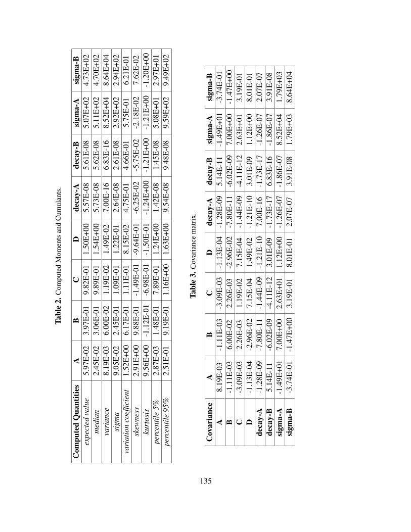
Tabl
e2.
Com
pute
dM
omen
tsan
dC
umul
ants
.
Com
pute
dQ
uant
ities
AB
CD
deca
y-A
deca
y-B
sigm
a-A
sigm
a-B
expe
cted
valu
e5.
97E
-02
3.97
E-0
19.
82E
-01
1.50
E+0
05.
57E
-08
5.61
E-0
85.
07E
+02
4.73
E+0
2m
edia
n2.
45E
-02
3.06
E-0
19.
89E
-01
1.54
E+0
05.
73E
-08
5.62
E-0
85.
11E
+02
4.70
E+0
2va
rian
ce8.
19E
-03
6.00
E-0
21.
19E
-02
1.49
E-0
27.
00E
-16
6.83
E-1
68.
52E
+04
8.64
E+0
4si
gma
9.05
E-0
22.
45E
-01
1.09
E-0
11.
22E
-01
2.64
E-0
82.
61E
-08
2.92
E+0
22.
94E
+02
vari
atio
nco
effic
ient
1.52
E+0
06.
17E
-01
1.11
E-0
18.
15E
-02
4.75
E-0
14.
66E
-01
5.75
E-0
16.
21E
-01
skew
ness
2.91
E+0
09.
88E
-01
-1.4
9E-0
1-9
.64E
-01
-6.2
5E-0
2-5
.75E
-02
-2.1
8E-0
27.
62E
-02
kurt
osis
9.56
E+0
0-1
.12E
-01
-6.9
8E-0
1-1
.50E
-01
-1.2
4E+0
0-1
.21E
+00
-1.2
1E+0
0-1
.20E
+00
perc
entil
e5%
2.87
E-0
31.
48E
-01
7.89
E-0
11.
24E
+00
1.42
E-0
81.
45E
-08
5.08
E+0
12.
97E
+01
perc
entil
e95
%2.
51E
-01
9.19
E-0
11.
16E
+00
1.63
E+0
09.
54E
-08
9.48
E-0
89.
59E
+02
9.49
E+0
2
Tabl
e3.
Cov
aria
nce
mat
rix.
Cov
aria
nce
AB
CD
deca
y-A
deca
y-B
sigm
a-A
sigm
a-B
A8.
19E
-03
-1.1
1E-0
3-3
.09E
-03
-1.1
3E-0
4-1
.28E
-09
5.14
E-1
1-1
.49E
+01
-3.7
4E-0
1B
-1.1
1E-0
36.
00E
-02
2.26
E-0
3-2
.96E
-02
-7.8
0E-1
1-6
.02E
-09
7.00
E+0
0-1
.47E
+00
C-3
.09E
-03
2.26
E-0
31.
19E
-02
7.15
E-0
4-1
.44E
-09
-4.1
1E-1
22.
63E
+01
3.19
E-0
1D
-1.1
3E-0
4-2
.96E
-02
7.15
E-0
41.
49E
-02
-1.2
1E-1
03.
01E
-09
1.12
E+0
08.
01E
-01
deca
y-A
-1.2
8E-0
9-7
.80E
-11
-1.4
4E-0
9-1
.21E
-10
7.00
E-1
6-1
.73E
-17
-1.2
6E-0
72.
07E
-07
deca
y-B
5.14
E-1
1-6
.02E
-09
-4.1
1E-1
23.
01E
-09
-1.7
3E-1
76.
83E
-16
-1.8
6E-0
73.
91E
-08
sigm
a-A
-1.4
9E+0
17.
00E
+00
2.63
E+0
11.
12E
+00
-1.2
6E-0
7-1
.86E
-07
8.52
E+0
41.
79E
+03
sigm
a-B
-3.7
4E-0
1-1
.47E
+00
3.19
E-0
18.
01E
-01
2.07
E-0
73.
91E
-08
1.79
E+0
38.
64E
+04
135
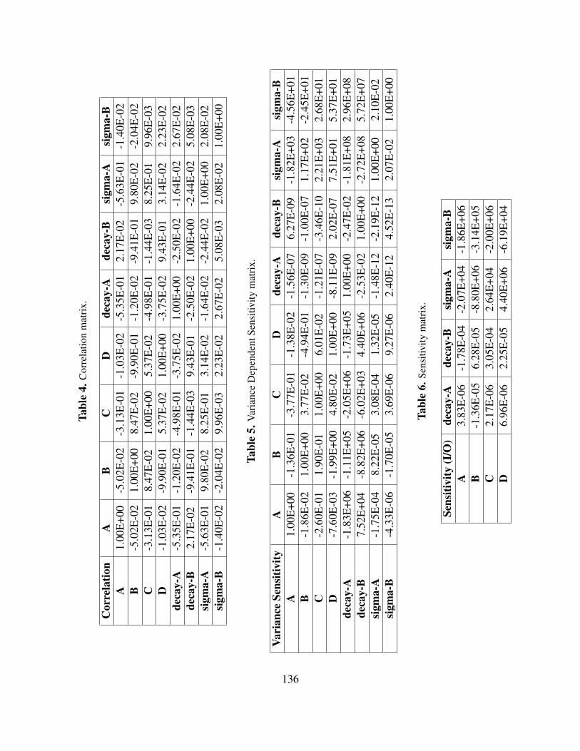
Tabl
e4.
Cor
rela
tion
mat
rix.
Cor
rela
tion
AB
CD
deca
y-A
deca
y-B
sigm
a-A
sigm
a-B
A1.
00E
+00
-5.0
2E-0
2-3
.13E
-01
-1.0
3E-0
2-5
.35E
-01
2.17
E-0
2-5
.63E
-01
-1.4
0E-0
2B
-5.0
2E-0
21.
00E
+00
8.47
E-0
2-9
.90E
-01
-1.2
0E-0
2-9
.41E
-01
9.80
E-0
2-2
.04E
-02
C-3
.13E
-01
8.47
E-0
21.
00E
+00
5.37
E-0
2-4
.98E
-01
-1.4
4E-0
38.
25E
-01
9.96
E-0
3D
-1.0
3E-0
2-9
.90E
-01
5.37
E-0
21.
00E
+00
-3.7
5E-0
29.
43E
-01
3.14
E-0
22.
23E
-02
deca
y-A
-5.3
5E-0
1-1
.20E
-02
-4.9
8E-0
1-3
.75E
-02
1.00
E+0
0-2
.50E
-02
-1.6
4E-0
22.
67E
-02
deca
y-B
2.17
E-0
2-9
.41E
-01
-1.4
4E-0
39.
43E
-01
-2.5
0E-0
21.
00E
+00
-2.4
4E-0
25.
08E
-03
sigm
a-A
-5.6
3E-0
19.
80E
-02
8.25
E-0
13.
14E
-02
-1.6
4E-0
2-2
.44E
-02
1.00
E+0
02.
08E
-02
sigm
a-B
-1.4
0E-0
2-2
.04E
-02
9.96
E-0
32.
23E
-02
2.67
E-0
25.
08E
-03
2.08
E-0
21.
00E
+00
Tabl
e5.
Var
ianc
eD
epen
dent
Sens
itivi
tym
atri
x.
Vari
ance
Sens
itivi
tyA
BC
Dde
cay-
Ade
cay-
Bsi
gma-
Asi
gma-
BA
1.00
E+0
0-1
.36E
-01
-3.7
7E-0
1-1
.38E
-02
-1.5
6E-0
76.
27E
-09
-1.8
2E+0
3-4
.56E
+01
B-1
.86E
-02
1.00
E+0
03.
77E
-02
-4.9
4E-0
1-1
.30E
-09
-1.0
0E-0
71.
17E
+02
-2.4
5E+0
1C
-2.6
0E-0
11.
90E
-01
1.00
E+0
06.
01E
-02
-1.2
1E-0
7-3
.46E
-10
2.21
E+0
32.
68E
+01
D-7
.60E
-03
-1.9
9E+0
04.
80E
-02
1.00
E+0
0-8
.11E
-09
2.02
E-0
77.
51E
+01
5.37
E+0
1de
cay-
A-1
.83E
+06
-1.1
1E+0
5-2
.05E
+06
-1.7
3E+0
51.
00E
+00
-2.4
7E-0
2-1
.81E
+08
2.96
E+0
8de
cay-
B7.
52E
+04
-8.8
2E+0
6-6
.02E
+03
4.40
E+0
6-2
.53E
-02
1.00
E+0
0-2
.72E
+08
5.72
E+0
7si
gma-
A-1
.75E
-04
8.22
E-0
53.
08E
-04
1.32
E-0
5-1
.48E
-12
-2.1
9E-1
21.
00E
+00
2.10
E-0
2si
gma-
B-4
.33E
-06
-1.7
0E-0
53.
69E
-06
9.27
E-0
62.
40E
-12
4.52
E-1
32.
07E
-02
1.00
E+0
0
Tabl
e6.
Sens
itivi
tym
atri
x.
Sens
itivi
ty(I
/O)
deca
y-A
deca
y-B
sigm
a-A
sigm
a-B
A3.
83E
-06
-1.7
8E-0
4-2
.07E
+04
-1.8
6E+0
6B
-1.3
6E-0
56.
28E
-05
-8.8
0E+0
6-3
.14E
+05
C2.
17E
-06
3.05
E-0
42.
64E
+04
-2.0
0E+0
6D
6.96
E-0
62.
25E
-05
4.40
E+0
6-6
.19E
+04
136
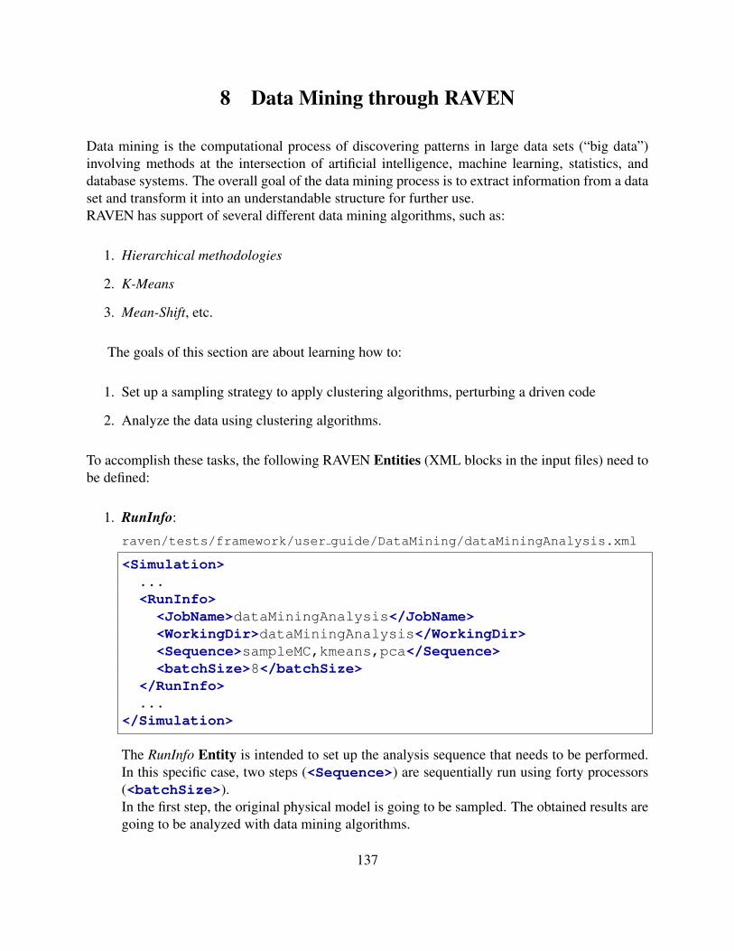
8 Data Mining through RAVEN
Data mining is the computational process of discovering patterns in large data sets (“big data”)involving methods at the intersection of artificial intelligence, machine learning, statistics, anddatabase systems. The overall goal of the data mining process is to extract information from a dataset and transform it into an understandable structure for further use.RAVEN has support of several different data mining algorithms, such as:
1. Hierarchical methodologies
2. K-Means
3. Mean-Shift, etc.
The goals of this section are about learning how to:
1. Set up a sampling strategy to apply clustering algorithms, perturbing a driven code
2. Analyze the data using clustering algorithms.
To accomplish these tasks, the following RAVEN Entities (XML blocks in the input files) need tobe defined:
1. RunInfo:
raven/tests/framework/user guide/DataMining/dataMiningAnalysis.xml
<Simulation>...<RunInfo>
<JobName>dataMiningAnalysis</JobName><WorkingDir>dataMiningAnalysis</WorkingDir><Sequence>sampleMC,kmeans,pca</Sequence><batchSize>8</batchSize>
</RunInfo>...
</Simulation>
The RunInfo Entity is intended to set up the analysis sequence that needs to be performed.In this specific case, two steps (<Sequence>) are sequentially run using forty processors(<batchSize>).In the first step, the original physical model is going to be sampled. The obtained results aregoing to be analyzed with data mining algorithms.
137

2. Files:raven/tests/framework/user guide/DataMining/dataMiningAnalysis.xml
<Simulation>...<Files>
<Input name="referenceInput.xml"type="input">referenceInput.xml</Input>
</Files>...
</Simulation>
Since the driven code uses a single input file, in this section the original input is placed. Theattribute name represents the alias that is going to be used in all the other input blocks inorder to refer to this file.
3. Models:raven/tests/framework/user guide/DataMining/dataMiningAnalysis.xml
<Simulation>...<Models><Code name="testModel" subType="GenericCode">
<executable>../physicalCode/analyticalbateman/AnalyticalDplMain.py</executable><clargs arg="python" type="prepend" /><clargs arg="" extension=".xml" type="input" /><clargs arg=" " extension=".csv" type="output" />
</Code><PostProcessor name="KMeans1" subType="DataMining">
<KDD labelFeature="klabels" lib="SciKitLearn"><SKLtype>cluster|KMeans</SKLtype><Features>A,B,C,D</Features><n_clusters>2</n_clusters><tol>1e-10</tol><random_state>1</random_state><init>k-means++</init><precompute_distances>True</precompute_distances>
</KDD></PostProcessor><PostProcessor name="PCA1" subType="DataMining">
<KDD lib="SciKitLearn"><Features>A,B,C,D</Features><SKLtype>decomposition|PCA</SKLtype><n_components>2</n_components>
</KDD></PostProcessor>
</Models>...
</Simulation>
The goal of this example is to show how the data mining algorithms in RAVEN can be usefulto analyze large data set.In addition to the previously explained Code model, two Post-Processor models (DataMining|cluster|KMeansandDataMining|decomposition|PCA) are specified. Note that the post-processing is per-formed on all the output FOMs used in this example ( A, B, C andD).
138
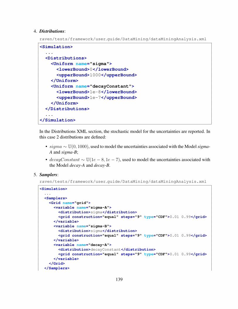
4. Distributions:
raven/tests/framework/user guide/DataMining/dataMiningAnalysis.xml
<Simulation>...<Distributions>
<Uniform name="sigma"><lowerBound>0</lowerBound><upperBound>1000</upperBound>
</Uniform><Uniform name="decayConstant">
<lowerBound>1e-8</lowerBound><upperBound>1e-7</upperBound>
</Uniform></Distributions>...
</Simulation>
In the Distributions XML section, the stochastic model for the uncertainties are reported. Inthis case 2 distributions are defined:
• sigma ∼ U(0, 1000), used to model the uncertainties associated with the Model sigma-A and sigma-B;
• decayConstant ∼ U(1e− 8, 1e− 7), used to model the uncertainties associated withthe Model decay-A and decay-B.
5. Samplers:raven/tests/framework/user guide/DataMining/dataMiningAnalysis.xml
<Simulation>...<Samplers>
<Grid name="grid"><variable name="sigma-A">
<distribution>sigma</distribution><grid construction="equal" steps="9" type="CDF">0.01 0.99</grid>
</variable><variable name="sigma-B">
<distribution>sigma</distribution><grid construction="equal" steps="9" type="CDF">0.01 0.99</grid>
</variable><variable name="decay-A">
<distribution>decayConstant</distribution><grid construction="equal" steps="9" type="CDF">0.01 0.99</grid>
</variable></Grid>
</Samplers>
139

...</Simulation>
In order to obtain the data-set on which the data mining algorithms are going to be applied,a Grid sampling approach is here employed.
6. DataObjects:
raven/tests/framework/user guide/DataMining/dataMiningAnalysis.xml
<Simulation>...<DataObjects>
<PointSet name="samples"><Input>decay-A,sigma-A,sigma-B</Input><Output>A,B,C,D</Output>
</PointSet><HistorySet name="histories">
<Input>sigma-A,sigma-B,decay-A</Input><Output>A,B,C,D,time</Output>
</HistorySet></DataObjects>...
</Simulation>
Int this block, two DataObjects are defined: 1) PointSet named “samples” used to collect thefinal outcomes of the code, 2) HistorySet named “histories” in which the full time responsesof the variables A,B,C,D are going to be stored.
7. OutStreams:
140
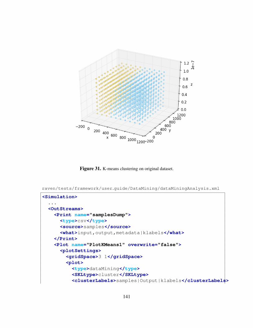
Figure 31. K-means clustering on original dataset.
raven/tests/framework/user guide/DataMining/dataMiningAnalysis.xml
<Simulation>...<OutStreams>
<Print name="samplesDump"><type>csv</type><source>samples</source><what>input,output,metadata|klabels</what>
</Print><Plot name="PlotKMeans1" overwrite="false">
<plotSettings><gridSpace>3 1</gridSpace><plot>
<type>dataMining</type><SKLtype>cluster</SKLtype><clusterLabels>samples|Output|klabels</clusterLabels>
141

<noClusters>2</noClusters><x>samples|Input|sigma-A</x><y>samples|Output|A</y><gridLocation>
<x>0</x><y>0</y>
</gridLocation><range>
<xmin>0</xmin><xmax>1000</xmax><ymin>0</ymin><ymax>1</ymax>
</range></plot><plot>
<type>dataMining</type><SKLtype>cluster</SKLtype><clusterLabels>samples|Output|klabels</clusterLabels><noClusters>2</noClusters><x>samples|Input|decay-A</x><y>samples|Output|A</y><gridLocation>
<x>1</x><y>0</y>
</gridLocation><range>
<xmin>1e-8</xmin><xmax>1e-7</xmax><ymin>0</ymin><ymax>1</ymax>
</range></plot><plot>
<type>dataMining</type><SKLtype>cluster</SKLtype><clusterLabels>samples|Output|klabels</clusterLabels><noClusters>2</noClusters><x>samples|Input|sigma-B</x><y>samples|Output|B</y><gridLocation>
<x>2</x><y>0</y>
142
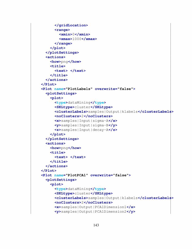
</gridLocation><range>
<xmin>0</xmin><xmax>1000</xmax>
</range></plot>
</plotSettings><actions><how>png</how><title>
<text> </text></title>
</actions></Plot><Plot name="PlotLabels" overwrite="false">
<plotSettings><plot>
<type>dataMining</type><SKLtype>cluster</SKLtype><clusterLabels>samples|Output|klabels</clusterLabels><noClusters>2</noClusters><x>samples|Input|sigma-A</x><y>samples|Input|sigma-B</y><z>samples|Input|decay-A</z>
</plot></plotSettings><actions><how>png</how><title>
<text> </text></title>
</actions></Plot><Plot name="PlotPCA1" overwrite="false">
<plotSettings><plot>
<type>dataMining</type><SKLtype>cluster</SKLtype><clusterLabels>samples|Output|klabels</clusterLabels><noClusters>2</noClusters><x>samples|Output|PCA1Dimension1</x><y>samples|Output|PCA1Dimension2</y>
143
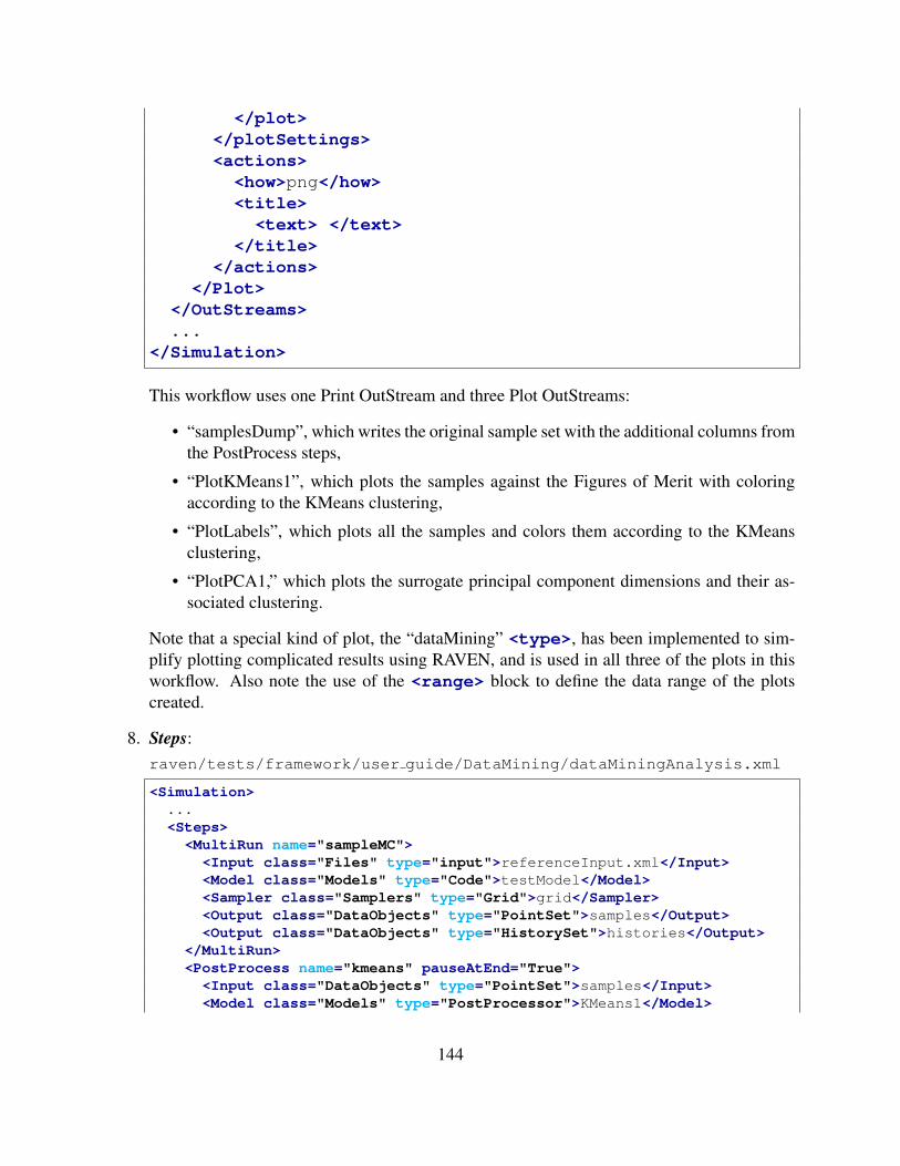
</plot></plotSettings><actions><how>png</how><title>
<text> </text></title>
</actions></Plot>
</OutStreams>...
</Simulation>
This workflow uses one Print OutStream and three Plot OutStreams:
• “samplesDump”, which writes the original sample set with the additional columns fromthe PostProcess steps,
• “PlotKMeans1”, which plots the samples against the Figures of Merit with coloringaccording to the KMeans clustering,
• “PlotLabels”, which plots all the samples and colors them according to the KMeansclustering,
• “PlotPCA1,” which plots the surrogate principal component dimensions and their as-sociated clustering.
Note that a special kind of plot, the “dataMining” <type>, has been implemented to sim-plify plotting complicated results using RAVEN, and is used in all three of the plots in thisworkflow. Also note the use of the <range> block to define the data range of the plotscreated.
8. Steps:raven/tests/framework/user guide/DataMining/dataMiningAnalysis.xml
<Simulation>...<Steps>
<MultiRun name="sampleMC"><Input class="Files" type="input">referenceInput.xml</Input><Model class="Models" type="Code">testModel</Model><Sampler class="Samplers" type="Grid">grid</Sampler><Output class="DataObjects" type="PointSet">samples</Output><Output class="DataObjects" type="HistorySet">histories</Output>
</MultiRun><PostProcess name="kmeans" pauseAtEnd="True"><Input class="DataObjects" type="PointSet">samples</Input><Model class="Models" type="PostProcessor">KMeans1</Model>
144
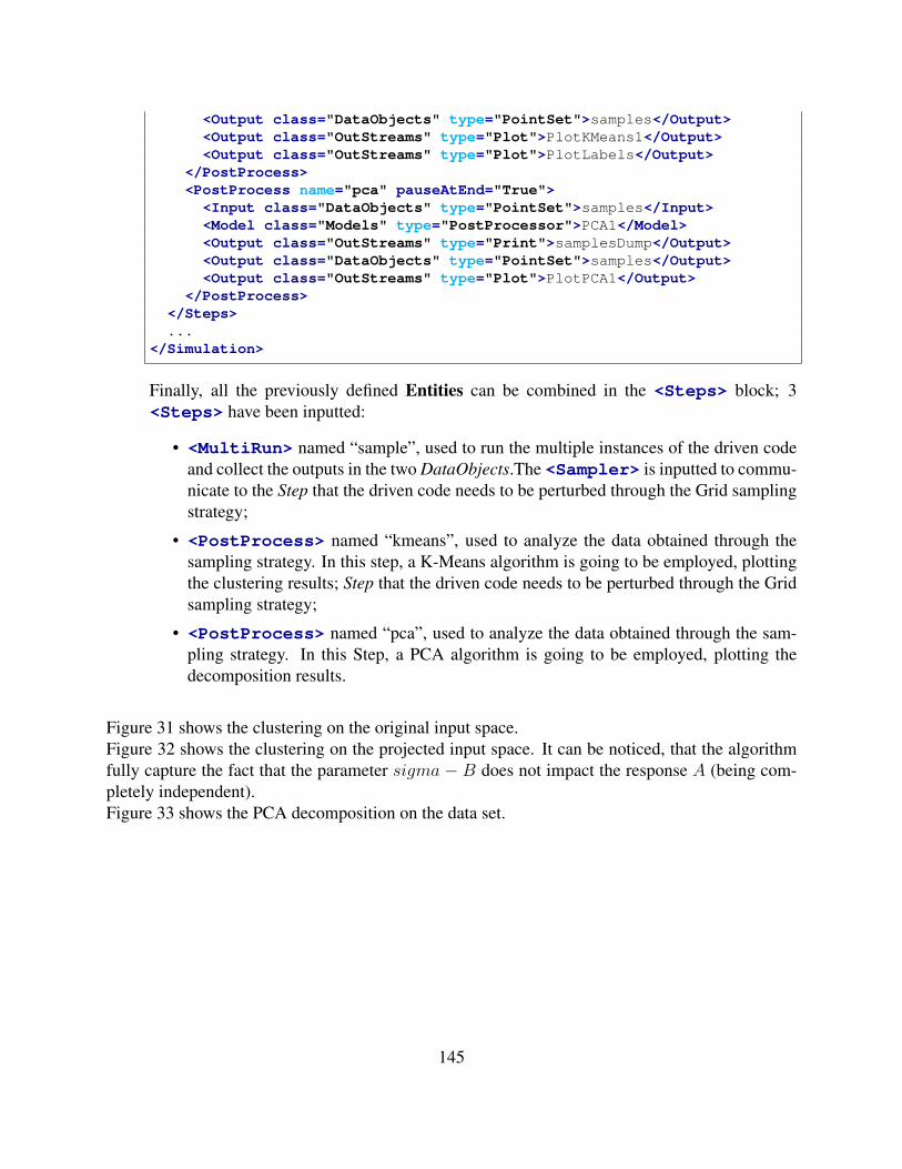
<Output class="DataObjects" type="PointSet">samples</Output><Output class="OutStreams" type="Plot">PlotKMeans1</Output><Output class="OutStreams" type="Plot">PlotLabels</Output>
</PostProcess><PostProcess name="pca" pauseAtEnd="True"><Input class="DataObjects" type="PointSet">samples</Input><Model class="Models" type="PostProcessor">PCA1</Model><Output class="OutStreams" type="Print">samplesDump</Output><Output class="DataObjects" type="PointSet">samples</Output><Output class="OutStreams" type="Plot">PlotPCA1</Output>
</PostProcess></Steps>...
</Simulation>
Finally, all the previously defined Entities can be combined in the <Steps> block; 3<Steps> have been inputted:
• <MultiRun> named “sample”, used to run the multiple instances of the driven codeand collect the outputs in the two DataObjects.The <Sampler> is inputted to commu-nicate to the Step that the driven code needs to be perturbed through the Grid samplingstrategy;
• <PostProcess> named “kmeans”, used to analyze the data obtained through thesampling strategy. In this step, a K-Means algorithm is going to be employed, plottingthe clustering results; Step that the driven code needs to be perturbed through the Gridsampling strategy;
• <PostProcess> named “pca”, used to analyze the data obtained through the sam-pling strategy. In this Step, a PCA algorithm is going to be employed, plotting thedecomposition results.
Figure 31 shows the clustering on the original input space.Figure 32 shows the clustering on the projected input space. It can be noticed, that the algorithmfully capture the fact that the parameter sigma − B does not impact the response A (being com-pletely independent).Figure 33 shows the PCA decomposition on the data set.
145

Figure 32. K-means clustering on projected parameters.
146
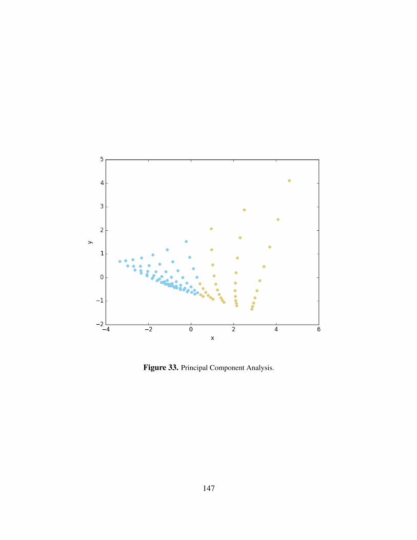
Figure 33. Principal Component Analysis.
147
9 Model Optimization
When analyzing the range of values obtainable by a model, frequently a key question is “whatset of parameters result in the best response value?” To answer this question, RAVEN uses the<Optimizer>, a powerful sampler-like entity that searches the input space to find minimum ormaximum values of a response.
In the remainder of this section, we will explore how to use the optimizer using a simpleanalytic problem, with a two-dimensional input space and single response of interest. After gettingused to running with the optimizer, we will add increasing complexity, including changing adaptivestep sizes, initial conditions, parallel trajectories, input space subdivision, input space constraints,and response constraints.
To demonstrate the operation of the Optimizer entities in RAVEN, the model we consider isthe Beale function, which is documented in the analytic tests for RAVEN and replicated here:
• Function: f(x, y) = (1.5− x+ xy)2 + (2.25− x+ xy2)2 + (2.625− x+ xy3)2
• Domain: −4.5 ≤ x, y ≤ 4.5
• Global Minimum: f(3, 0.5) = 0
The two inputs are the variables x and y, and the response is a value we’ll assign to ans, shortfor “answer”. The model is an external model in RAVEN, and can be found at
raven/tests/framework/AnalyticModes/optimizing/beale.py.
The function’s values are distributed as in Fig. 34.
Note that throughout this example we use the SPSA optimizer by way of demonstration, sinceit is the first advanced algorithm for optimization included in RAVEN; many of the options andparameters apply to other optimizers, and details can be found in the RAVEN user manual.
9.1 Introduction: The Optimizer Input
As with other entities, the Optimizer gets its own XML block in the RAVEN input. Here’s anexample of an input for a SPSA optimizer named ’opter’:
148

Figure 34. Plot of Beale’s function for Optimization
raven/tests/framework/user guide/optimizing/simple.xml
<Simulation>...<Optimizers><SPSA name="opter">
<initialization><initialSeed>1234</initialSeed>
</initialization><TargetEvaluation class="DataObjects" type="PointSet">optOut</TargetEvaluation><variable name="x">
<upperBound>4.5</upperBound><lowerBound>-4.5</lowerBound><initial>0</initial>
</variable><variable name="y">
<upperBound>4.5</upperBound><lowerBound>-4.5</lowerBound><initial>0</initial>
</variable><objectVar>ans</objectVar>
</SPSA></Optimizers>...
</Simulation>
149

This is the smallest amount of input needed to run an optimization problem, with the exceptionthat we include the <initialSeed> to maintain consistent results. Note the required blocksincluded to define the optimizer:
• <TargetEvaluation>, which declares the DataObject that the optimization search eval-uations are going to be placed in. All of the optimal points found as part of the optimization,as well as any other points evaluated as part of the algorithm, are placed in this object so theoptimizer can retrieve this information later. When this data object is defined, it is criticalthat the objective variable is defined in the output space, and the input variables in the inputspace, so the optimizer can collect the results of its sampling. The data object type shouldbe “PointSet” for this data object. In this example, we use the self-descriptive optOut dataobject.
• <variable>, which is where you can define the input space variables, one for each ofthese nodes. Declaring a variable here informs the optimizer that you want it to find theoptimal value for this variable, along with the other variables declared in their own blocks.Additionally, you define the upper and lower bounds of the variable, which will give theoptimizer some general expectations for finding the optimal point; it will never try to samplea value smaller than the lower bound or larger than the upper bound. In the example wedefine variables x and y as our input variables, and both of them coincidentally range between-4.5 and 4.5. We set the initial values for both variables to 0 through the <initial>block, which is required in most cases; the exception is when a preconditioner sets them inmulitlevel optimization, but we’re not concerned with that feature at this point.
• <objectVar>, which is where you indicate the variable for which you want to find theminimum (or, if you change the default, maximum). As listed here, we want to minimize thevalue of ans given a range of possible values for x and y.
The other critical blocks in this input are as follows:
9.1.1 Models
raven/tests/framework/user guide/optimizing/simple.xml<Simulation>...<Models>
<ExternalModel ModuleToLoad="../../../../framework/AnalyticModels/optimizing/beale" name="beale" subType=""><variables>x,y,ans</variables>
</ExternalModel></Models>...
</Simulation>
Note that we define the external model with the name ’beale’ and provide a path to the analyticmodel itself. This model is set up with the run method that allows RAVEN to run the model. Wealso list all our input/output variables, x, y, and ans.
150
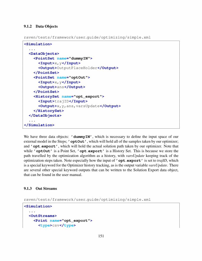
9.1.2 Data Objects
raven/tests/framework/user guide/optimizing/simple.xml
<Simulation>...<DataObjects>
<PointSet name="dummyIN"><Input>x,y</Input><Output>OutputPlaceHolder</Output>
</PointSet><PointSet name="optOut">
<Input>x,y</Input><Output>ans</Output>
</PointSet><HistorySet name="opt_export">
<Input>trajID</Input><Output>x,y,ans,varsUpdate</Output>
</HistorySet></DataObjects>...
</Simulation>
We have three data objects: ’dummyIN’, which is necessary to define the input space of ourexternal model in the Steps; ’optOut’, which will hold all of the samples taken by our optimizer;and ’opt export’, which will hold the actual solution path taken by our optimizer. Note thatwhile ’optOut’ is a Point Set, ’opt export’ is a History Set. This is because we store thepath travelled by the optimization algorithm as a history, with varsUpdate keeping track of theoptimization steps taken. Note especially how the input of ’opt export’ is set to trajID, whichis a special keyword for the Optimizer history tracking, as is the output variable varsUpdate. Thereare several other special keyword outputs that can be written to the Solution Export data object,that can be found in the user manual.
9.1.3 Out Streams
raven/tests/framework/user guide/optimizing/simple.xml
<Simulation>...<OutStreams>
<Print name="opt_export"><type>csv</type>
151

<source>opt_export</source></Print>
</OutStreams>...
</Simulation>
Here we define the way to print the output of our optimization algorithm. There’s not much tonote, except that we’ll be printing the optimization path as a History-based CSV.
9.1.4 Steps
raven/tests/framework/user guide/optimizing/simple.xml
<Simulation>...<Steps><MultiRun name="optimize">
<Input class="DataObjects" type="PointSet">dummyIN</Input><Model class="Models" type="ExternalModel">beale</Model><Optimizer class="Optimizers" type="SPSA">opter</Optimizer><SolutionExport class="DataObjects" type="HistorySet">opt_export</SolutionExport><Output class="DataObjects" type="PointSet">optOut</Output>
</MultiRun><IOStep name="print">
<Input class="DataObjects" type="HistorySet">opt_export</Input><Output class="OutStreams" type="Print">opt_export</Output>
</IOStep></Steps>...
</Simulation>
Here we put it all together into a work flow that RAVEN can follow. We only need two steps: oneto optimize, and one to print out the results. To actually perform the optimization, we need a Mul-tiRun step, which we cleverly name ’optimize’. For input we take the placeholder data objectdummyIN, which sets up the input space of the model we defined, beal. Where a <Sampler>would normally go, we include the <Optimizer> we defined earlier. We output to the same dataobject we indicated in the Optimizer’s <TargetEvaluation> node. Finally, we note specifi-cally the use of the <SolutionExport> node. The data object defined in this node is where theOptimizer will write the optimization path history, with the final entry being the last step taken bythe optimizer. The IOStep is unremarkable, used simply to write out the optimization path historyto file.
9.1.5 Conclusion
After reviewing the components (don’t forget the RunInfo block!), you can run this example andsee the results. In particular, we can view the history of the optimizer in Simple/opt export 0.csv.
152

Note that opt export is the name of the <Print> OutStream we defined in the input file, andthe 0 indicates this is the first optimization path followed (we’ll cover multiple paths later insection 9.2).
When we open the file (preferably in a CSV reader such a spreadsheet viewer), we see a CSVwith four headers, the outputs defined in the data object in the input file: x, y, ans, and varsUpdate(not necessarily in that order). x, y, and ans are the values of the variable at each optimizationiteration, while varsUpdate gives the sequential order of the optimization iteration.
If we look at the last line, we converged around f(1.61,−0.189) = 1.67, which is okay butstill quite a ways from the analytic optimal point f(3, 0.5) = 0. If we look at the output from therun, we can look at the last time RAVEN was “Checking convergence for Trajectory 0”. Belowthat statement, there are a series of convergence criteria and their status. We can see that the reasonwe converged at the end is the Relative Loss Diff, which means the relative change inthe response ans was sufficiently small between steps to cause convergence. Clearly, we claimedconvergence prematurely because of the default convergence values used by the optimizer. Becausethese convergence criteria are very problem-specific, the default parameters will not work best forall problems.
We can improve this result by changing convergence parameters as well as step size growthand shrink factors, all of which can be found in the user manual, and many of which we’ll discussin the rest of this section.
9.2 Initial Conditions and Parallel Trajectories
Notice we set the optimization search to start at (0, 0). You can change this initial value throughthe <initial> block within the <variable> definition node.
Furthermore, RAVEN offers the possibility to run multiple optimization paths in parallel. Be-cause many (perhaps most) optimization techniques get stuck in local minima, using multiple paths(or trajectories as they are called in RAVEN) increases the likelihood that one of the trajectorieswill find the global minimum point. You can request multiple trajectories by providing a variety ofinitial conditions in the <initial> block, as shown in this Optimizer example:
raven/tests/framework/user guide/optimizing/multiple trajectories.xml
<Simulation>...<Optimizers><SPSA name="opter">
<initialization><initialSeed>1234</initialSeed>
</initialization><TargetEvaluation class="DataObjects" type="PointSet">optOut</TargetEvaluation><variable name="x">
<upperBound>4.5</upperBound><lowerBound>-4.5</lowerBound>
153
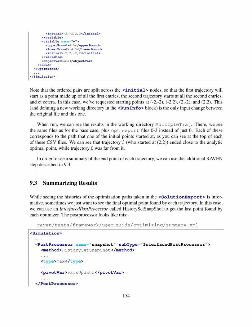
<initial>-2,-2,2,2</initial></variable><variable name="y">
<upperBound>4.5</upperBound><lowerBound>-4.5</lowerBound><initial>-2,2,-2,2</initial>
</variable><objectVar>ans</objectVar>
</SPSA></Optimizers>...
</Simulation>
Note that the ordered pairs are split across the <initial> nodes, so that the first trajectory willstart as a point made up of all the first entries, the second trajectory starts at all the second entries,and et cetera. In this case, we’ve requested starting points at (-2,-2), (-2,2), (2,-2), and (2,2). This(and defining a new working directory in the <RunInfo> block) is the only input change betweenthe original file and this one.
When run, we can see the results in the working directory MultipleTraj. There, we seethe same files as for the base case, plus opt export files 0-3 instead of just 0. Each of thesecorresponds to the path that one of the initial points started at, as you can see at the top of eachof these CSV files. We can see that trajectory 3 (who started at (2,2)) ended close to the analyticoptimal point, while trajectory 0 was far from it.
In order to see a summary of the end point of each trajectory, we can use the additional RAVENstep described in 9.3.
9.3 Summarizing Results
While seeing the histories of the optimization paths taken in the <SolutionExport> is infor-mative, sometimes we just want to see the final optimal point found by each trajectory. In this case,we can use an InterfacedPostProcessor called HistorySetSnapShot to get the last point found byeach optimizer. The postprocessor looks like this:
raven/tests/framework/user guide/optimizing/summary.xml
<Simulation>...<PostProcessor name="snapshot" subType="InterfacedPostProcessor"><method>HistorySetSnapShot</method>...<type>max</type>...<pivotVar>varsUpdate</pivotVar>...
</PostProcessor>
154

...</Simulation>
Note that we named the postprocessor ’snapshot’, and instructed it to look for the ’max’value of ’varsUpdate’ in each of the histories, and combine them into a single data set. Weadd the following Step to our <Steps> to run it:
raven/tests/framework/user guide/optimizing/summary.xml
<Simulation>...<PostProcess name="getOptPoint"><Input class="DataObjects" type="HistorySet">opt_export</Input>...<Model class="Models" type="PostProcessor">snapshot</Model>...<Output class="DataObjects" type="PointSet">opt_soln</Output>...
</PostProcess>...
</Simulation>
Don’t forget to add ’getOptPoint’ to the <Sequence> in the <RunInfo> block, before’print’ but after ’optimize’. Note that this post-processing step takes the <SolutionExport>data object from the optimizing step as input, runs the postprocessing model, then places the resultsin a new data object, ’opt soln’, which we add to the <DataObjects> list in the input file.
Note also that we added the printing of the ’opt soln’ data object to the ’print’ <IOStep>;we only needed to write an <OutStream> for it, not a whole new step.
After running this input, you can open Summary/opt soln.csv to see the final results ofeach optimization trajectory. The variable trajID gives the trajectory label, x and y give the finallocation of the optimal point found by that trajectory, ans gives the value of the response at thatlocation, and varsUpdate shows how many iterations were necessary to find that optimal point.The trajectory with the lowest value for ans is the most optimal point found.
9.4 Adjusting Adaptive Steps
As we’ve seen, some of the optimization paths are struggling to converge to meaningful optimalsolutions. One way to improve this is to tinker with the convergence tolerances defined in the usermanual. Another is to change the step size modifications used as part of the search process, whichwe discuss in this section. First, we briefly discuss how the SPSA chooses its step size, so we canmake informed choices about what parameters to use.
155

Because SPSA is a gradient-based method, it operates by starting at a particular point, estimat-ing the gradient at that point, then taking a step in the opposite direction of the gradient in orderto follow a downhill path. It adaptively chooses how long of a step to take based on its history.If the gradient is in the same direction twice in a row, the algorithm assumes there’s further totravel, so increases its step size multiplicatively by the grainGrowthFactor, which by default is 2.0in RAVEN. If, on the other hand, the gradient switches directions, then the step size is dividedby the gainShrinkFactor, which again is 2.0 by default in RAVEN. This means that by default, ifthe gradient keeps going in the same direction, you always double your step size, while if you’rebouncing back and forth in a valley, the step size is halved at each iteration.
By way of note, in higher dimensions, the actual growth or shrink multiplier is scaled by a dotproduct between the two previous gradients, with a max of the grain growth factor when the dotproduct is 1 (exactly aligned) and a minimum of grain shrink factor when the dot product is -1(exactly opposite). This means if the gradient is at right angles with the past gradient, then the stepsize remains unchanged (dot product is 0).
There are some additional considerations for the step size change, as well. If the algorithmtakes a step, then discovers the new point has a worse response value than the point it’s at, it willreject the new point, re-evaluate the gradient, and flag the step size to be divided by the gain shrinkfactor. Because of this, if the gain shrink factor is too large, false convergence can be obtainedwhen the algorithm struggles to find a new downhill point to move to. As a result, in practice it isoften beneficial to have a gain shrink factor that is smaller than the gain growth factor.
For this particular example, we use gain growth factor of 1.5 (meaning when the gradientcontinues in the same direction our step grows to 150% of its old value) and a gain shrink factor of1.25 (meaning when the gradient flips directions our step size shrinks to 80% of its old value). Weadd this to the base case (simple.xml) to get:
raven/tests/framework/user guide/optimizing/step size.xml
<Simulation>...<Optimizers><SPSA name="opter">
<initialization><initialSeed>1234</initialSeed>
</initialization><TargetEvaluation class="DataObjects" type="PointSet">optOut</TargetEvaluation><convergence>
<gainGrowthFactor>1.5</gainGrowthFactor><gainShrinkFactor>1.25</gainShrinkFactor>
</convergence><variable name="x">
<upperBound>4.5</upperBound><lowerBound>-4.5</lowerBound><initial>0</initial>
</variable><variable name="y">
<upperBound>4.5</upperBound><lowerBound>-4.5</lowerBound><initial>0</initial>
</variable>
156
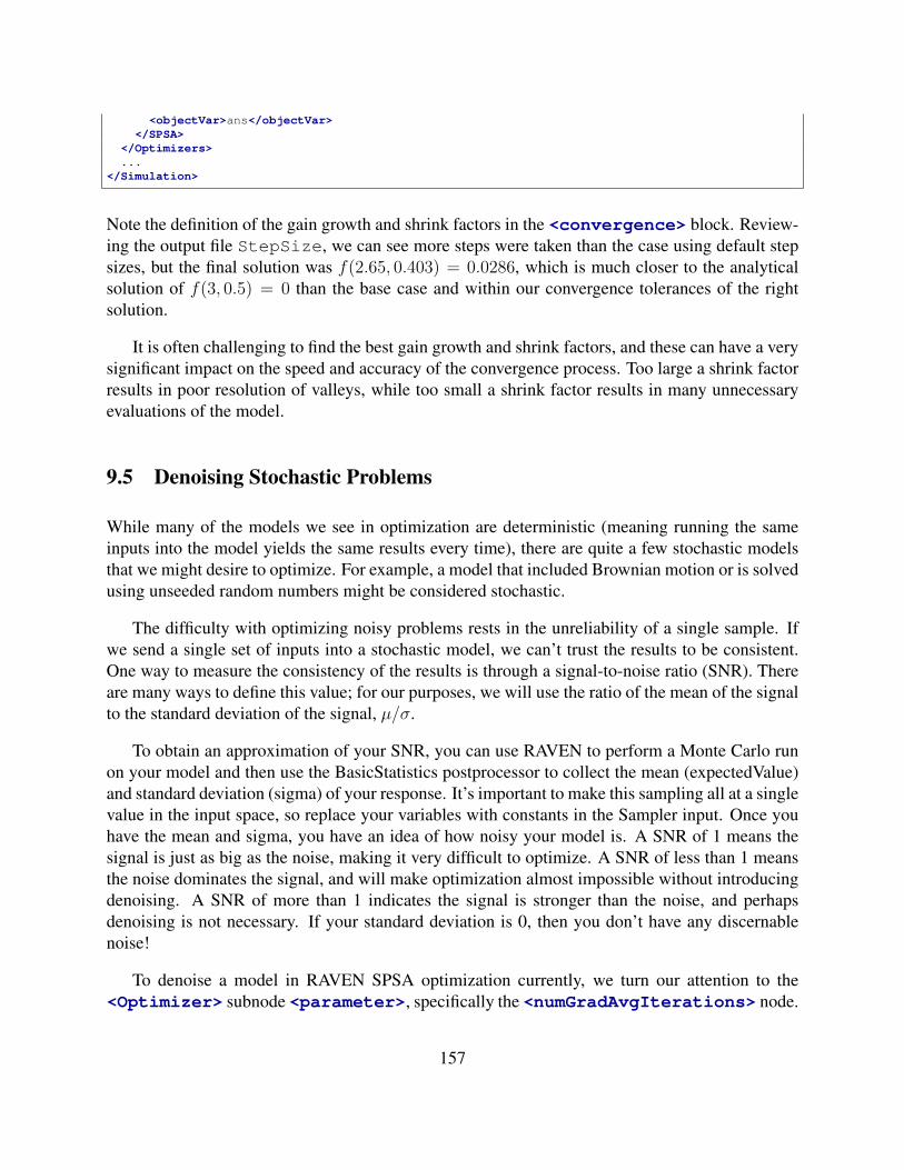
<objectVar>ans</objectVar></SPSA>
</Optimizers>...
</Simulation>
Note the definition of the gain growth and shrink factors in the <convergence> block. Review-ing the output file StepSize, we can see more steps were taken than the case using default stepsizes, but the final solution was f(2.65, 0.403) = 0.0286, which is much closer to the analyticalsolution of f(3, 0.5) = 0 than the base case and within our convergence tolerances of the rightsolution.
It is often challenging to find the best gain growth and shrink factors, and these can have a verysignificant impact on the speed and accuracy of the convergence process. Too large a shrink factorresults in poor resolution of valleys, while too small a shrink factor results in many unnecessaryevaluations of the model.
9.5 Denoising Stochastic Problems
While many of the models we see in optimization are deterministic (meaning running the sameinputs into the model yields the same results every time), there are quite a few stochastic modelsthat we might desire to optimize. For example, a model that included Brownian motion or is solvedusing unseeded random numbers might be considered stochastic.
The difficulty with optimizing noisy problems rests in the unreliability of a single sample. Ifwe send a single set of inputs into a stochastic model, we can’t trust the results to be consistent.One way to measure the consistency of the results is through a signal-to-noise ratio (SNR). Thereare many ways to define this value; for our purposes, we will use the ratio of the mean of the signalto the standard deviation of the signal, µ/σ.
To obtain an approximation of your SNR, you can use RAVEN to perform a Monte Carlo runon your model and then use the BasicStatistics postprocessor to collect the mean (expectedValue)and standard deviation (sigma) of your response. It’s important to make this sampling all at a singlevalue in the input space, so replace your variables with constants in the Sampler input. Once youhave the mean and sigma, you have an idea of how noisy your model is. A SNR of 1 means thesignal is just as big as the noise, making it very difficult to optimize. A SNR of less than 1 meansthe noise dominates the signal, and will make optimization almost impossible without introducingdenoising. A SNR of more than 1 indicates the signal is stronger than the noise, and perhapsdenoising is not necessary. If your standard deviation is 0, then you don’t have any discernablenoise!
To denoise a model in RAVEN SPSA optimization currently, we turn our attention to the<Optimizer> subnode <parameter>, specifically the <numGradAvgIterations> node.
157
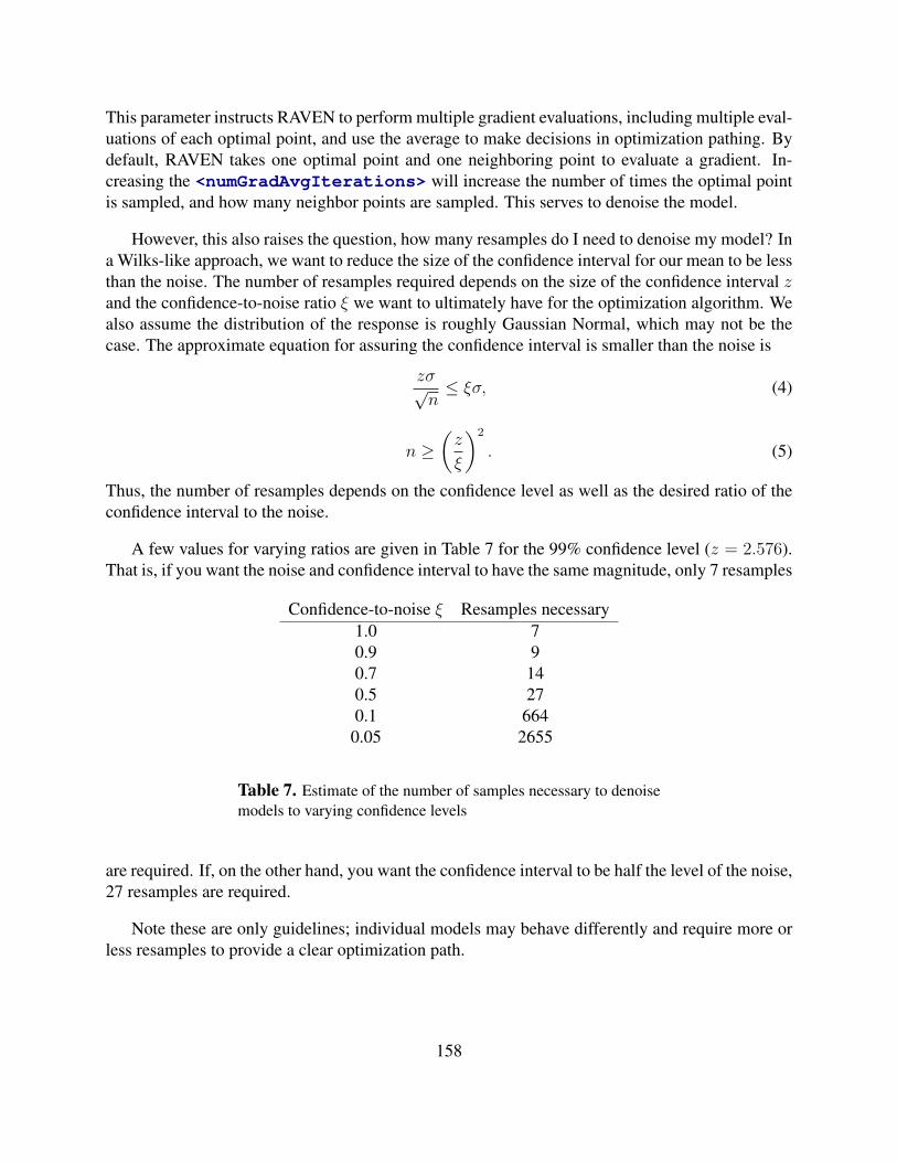
This parameter instructs RAVEN to perform multiple gradient evaluations, including multiple eval-uations of each optimal point, and use the average to make decisions in optimization pathing. Bydefault, RAVEN takes one optimal point and one neighboring point to evaluate a gradient. In-creasing the <numGradAvgIterations> will increase the number of times the optimal pointis sampled, and how many neighbor points are sampled. This serves to denoise the model.
However, this also raises the question, how many resamples do I need to denoise my model? Ina Wilks-like approach, we want to reduce the size of the confidence interval for our mean to be lessthan the noise. The number of resamples required depends on the size of the confidence interval zand the confidence-to-noise ratio ξ we want to ultimately have for the optimization algorithm. Wealso assume the distribution of the response is roughly Gaussian Normal, which may not be thecase. The approximate equation for assuring the confidence interval is smaller than the noise is
zσ√n≤ ξσ, (4)
n ≥(z
ξ
)2
. (5)
Thus, the number of resamples depends on the confidence level as well as the desired ratio of theconfidence interval to the noise.
A few values for varying ratios are given in Table 7 for the 99% confidence level (z = 2.576).That is, if you want the noise and confidence interval to have the same magnitude, only 7 resamples
Confidence-to-noise ξ Resamples necessary1.0 70.9 90.7 140.5 270.1 664
0.05 2655
Table 7. Estimate of the number of samples necessary to denoisemodels to varying confidence levels
are required. If, on the other hand, you want the confidence interval to be half the level of the noise,27 resamples are required.
Note these are only guidelines; individual models may behave differently and require more orless resamples to provide a clear optimization path.
158
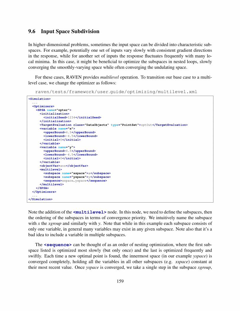
9.6 Input Space Subdivision
In higher-dimensional problems, sometimes the input space can be divided into characteristic sub-spaces. For example, potentially one set of inputs vary slowly with consistent gradient directionsin the response, while for another set of inputs the response fluctuates frequently with many lo-cal minima. In this case, it might be beneficial to optimize the subspaces in nested loops, slowlyconverging the smoothly-varying space while often converging the undulating space.
For these cases, RAVEN provides multilevel operation. To transition our base case to a multi-level case, we change the optimizer as follows:
raven/tests/framework/user guide/optimizing/multilevel.xml
<Simulation>...<Optimizers><SPSA name="opter">
<initialization><initialSeed>1234</initialSeed>
</initialization><TargetEvaluation class="DataObjects" type="PointSet">optOut</TargetEvaluation><variable name="x">
<upperBound>4.5</upperBound><lowerBound>-4.5</lowerBound><initial>0</initial>
</variable><variable name="y">
<upperBound>4.5</upperBound><lowerBound>-4.5</lowerBound><initial>0</initial>
</variable><objectVar>ans</objectVar><multilevel>
<subspace name="xspace">x</subspace><subspace name="yspace">y</subspace><sequence>xspace,yspace</sequence>
</multilevel></SPSA>
</Optimizers>...
</Simulation>
Note the addition of the <multilevel> node. In this node, we need to define the subspaces, thenthe ordering of the subspaces in terms of convergence priority. We intuitively name the subspacewith x the xgroup and similarly with y. Note that while in this example each subspace consists ofonly one variable, in general many variables may exist in any given subspace. Note also that it’s abad idea to include a variable in multiple subspaces.
The <sequence> can be thought of as an order of nesting optimization, where the first sub-space listed is optimized most slowly (but only once) and the last is optimized frequently andswiftly. Each time a new optimal point is found, the innermost space (in our example yspace) isconverged completely, holding all the variables in all other subspaces (e.g. xspace) constant attheir most recent value. Once yspace is converged, we take a single step in the subspace xgroup,
159
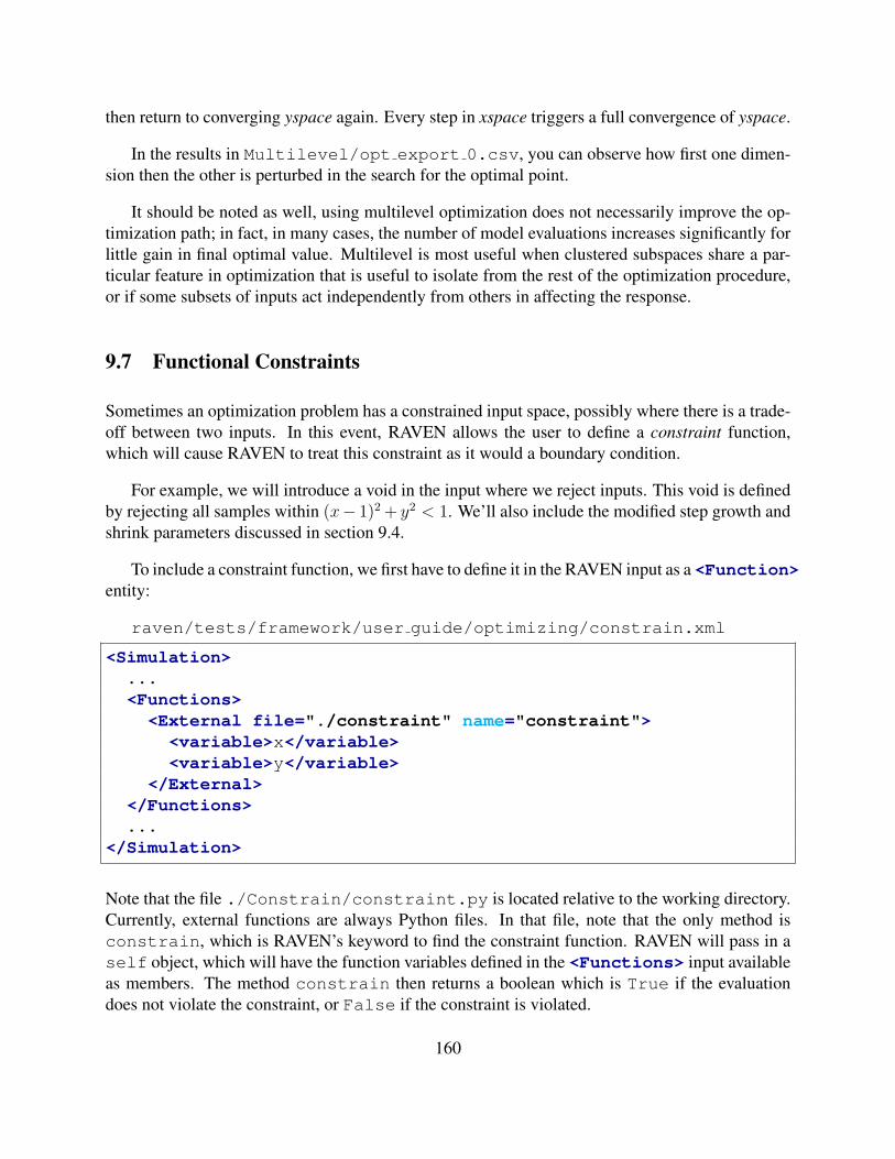
then return to converging yspace again. Every step in xspace triggers a full convergence of yspace.
In the results in Multilevel/opt export 0.csv, you can observe how first one dimen-sion then the other is perturbed in the search for the optimal point.
It should be noted as well, using multilevel optimization does not necessarily improve the op-timization path; in fact, in many cases, the number of model evaluations increases significantly forlittle gain in final optimal value. Multilevel is most useful when clustered subspaces share a par-ticular feature in optimization that is useful to isolate from the rest of the optimization procedure,or if some subsets of inputs act independently from others in affecting the response.
9.7 Functional Constraints
Sometimes an optimization problem has a constrained input space, possibly where there is a trade-off between two inputs. In this event, RAVEN allows the user to define a constraint function,which will cause RAVEN to treat this constraint as it would a boundary condition.
For example, we will introduce a void in the input where we reject inputs. This void is definedby rejecting all samples within (x− 1)2+ y2 < 1. We’ll also include the modified step growth andshrink parameters discussed in section 9.4.
To include a constraint function, we first have to define it in the RAVEN input as a <Function>entity:
raven/tests/framework/user guide/optimizing/constrain.xml
<Simulation>...<Functions>
<External file="./constraint" name="constraint"><variable>x</variable><variable>y</variable>
</External></Functions>...
</Simulation>
Note that the file ./Constrain/constraint.py is located relative to the working directory.Currently, external functions are always Python files. In that file, note that the only method isconstrain, which is RAVEN’s keyword to find the constraint function. RAVEN will pass in aself object, which will have the function variables defined in the <Functions> input availableas members. The method constrain then returns a boolean which is True if the evaluationdoes not violate the constraint, or False if the constraint is violated.
160
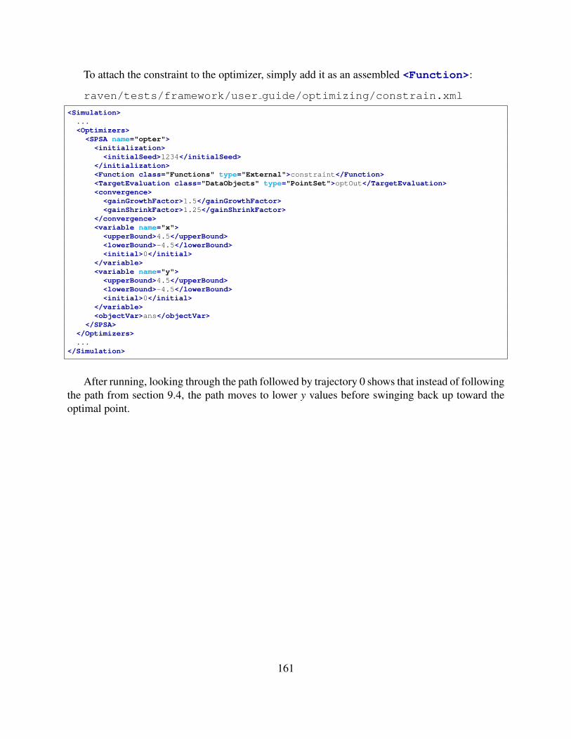
To attach the constraint to the optimizer, simply add it as an assembled <Function>:
raven/tests/framework/user guide/optimizing/constrain.xml
<Simulation>...<Optimizers><SPSA name="opter">
<initialization><initialSeed>1234</initialSeed>
</initialization><Function class="Functions" type="External">constraint</Function><TargetEvaluation class="DataObjects" type="PointSet">optOut</TargetEvaluation><convergence>
<gainGrowthFactor>1.5</gainGrowthFactor><gainShrinkFactor>1.25</gainShrinkFactor>
</convergence><variable name="x">
<upperBound>4.5</upperBound><lowerBound>-4.5</lowerBound><initial>0</initial>
</variable><variable name="y">
<upperBound>4.5</upperBound><lowerBound>-4.5</lowerBound><initial>0</initial>
</variable><objectVar>ans</objectVar>
</SPSA></Optimizers>...
</Simulation>
After running, looking through the path followed by trajectory 0 shows that instead of followingthe path from section 9.4, the path moves to lower y values before swinging back up toward theoptimal point.
161

10 EnsembleModel
In most RAVEN MultiRun steps, a sampler provides a variety of inputs to a model, whose outputsthen produce a set of responses that can be used in many ways. However, sometimes a singlemodel is insufficient to produce the response we want. When this happens, the EnsembleModelopens up a new vista of simulation options.
The EnsembleModel is a powerful tool for chaining multiple models together, with outputs ofsome models becoming inputs for others. Whether this is adding a preprocessing or postprocess-ing model, or linking multiple physics-based models together, the EnsembleModel provides thefunctionality to see many models together as a single model in a MultiRun step.
Note that the EnsembleModel combines multiple models for each sample; that is, the wholeensemble of models is run for each sample taken by RAVEN. If instead you want to postprocess abatch of sampled data, try the PostProcessor models instead.
10.1 Introduction: The EnsembleModel
The key to the EnsembleModel is careful definition of the inputs and outputs of each model. Whenan EnsembleModel is defined in a RAVEN run, RAVEN will automatically scan the inputs andoutputs of each model and determine the right order to evaluate the models in (or graph).
10.2 Example: ballistics and impact
As a basic example, consider two physics models. The first is a ballistics code, used to determinethe kinetic energy E of a ball when it hits the ground, with a path depending on its initial heighty0, initial velocity v0, mass m and initial angle θ0. We’ll assume we’re near the Earth’s surface andaside from the initial launch height, we’re launching over a flat surface. This can be represented asa functional E(y0, v0,m, θ0).
The second physics model is an impact code that estimates the diameter of the crater D madewhen a ball impacts. With a few simplifying assumptions (D is under 1 km, the impact is nearEarth’s surface, the impact is in dry sand with fixed density), sizeD can be determined as a functionof the ball’s kinetic energy when impacting E, its mass m, and its radius r: D(E,m, r).
We can see that the input E for the impact model is calculated by the ballistics code. InRAVEN the EnsembleModel will automatically detect this, and run the ballistics code before theimpact code in each iteration.
In general, the EnsembleModel also has some finite capacity for resolving circular dependen-
162

cies using Picard iteration. See the manual for more information on this capability.
Setting up an EnsembleModel can be more complex than other models, so we’ll walk throughthe input using our example outlined above. For our purposes, we’re going to let RAVEN perturbthe codes using the GenericCode interface. We’ll call the ballistics code ballistics.py withkeyword input file ballistics input.txt and similarly the impact code impact.py withkeyword input file impact input.txt.
The RAVEN input file for this example is located at
raven/tests/framework/user_guide/EnsembleModel/basic.xml
with run directory run basic. The models and inputs are in the run directory.
Now we turn our attention to the RAVEN input file. We will discuss <DataObjects>,<Files>, <Models>, and <Steps> in detail; the rest are typical usage and need no specialattention.
10.2.1 DataObjects
The key to a successful EnsembleModel is setting up the DataObject inputs and outputs. Eachmodel has a <TargetEvaluation> DataObject that specifies what the inputs and outputs arefor that model. In addition, any <Output> DataObjects in the <MultiRun> step can collect anyor all of the variables used throughout the EnsembleModel calculation, either as inputs or outputs.
In this example, our convention is to name the <TargetEvaluation> DataObjects as’model data’, replacing ’model’ with the model name. Additionally, we add a DataObjectto store the final results of the <MultiRun> step:
raven/tests/framework/user guide/EnsembleModel/basic.xml
<Simulation>...<DataObjects>
<PointSet name="ballistics_data"><Input>y0,v0,ang,m</Input><Output>E</Output>
</PointSet><PointSet name="impact_data">
<Input>E,m,r</Input><Output>D</Output>
</PointSet><PointSet name="final_results">
163

<Input>y0,v0,ang,m,r</Input><Output>E,D</Output>
</PointSet></DataObjects>...
</Simulation>
In this example, we see three DataObjects. ’ballistics data’ determines the inputs andoutputs of the ballistics.py model, so for its input space we have y0,v0,ang,m, whichcorrespond to y0, v0, θ0,m; for the output, we have E (for E).
The second DataObject, ’impact data’, delineates the inputs and outputs of the impact.pymodel, so for its input space we have E,m,r, while in the output space we have D. RAVEN willuse these first two DataObjects to map the order in which these two models should be run (firstballistics, then impact) and transfer data from one to the next.
The third DataObject, ’final results’, can contain any information we want it to. In thiscase, we want to collect all the variables in their original spaces, so we take y0,v0,ang,m,r asinputs and E,D as outputs.
10.2.2 Files
Since we know both of our models take input files to set the variable values, we inform RAVENabout the template input files and give those files RAVEN names in the <Files> block. In this ex-ample, our input file for ballistics.py is ballistics template.txt, which we simplyname ’ballistics input’. Similarly, for impact.py the input file is impact template.txt,which we name ’impact input’:
raven/tests/framework/user guide/EnsembleModel/basic.xml
<Simulation>...<Files><Input name="ballistics_input">ballistics_template.txt</Input><Input name="impact_input">impact_template.txt</Input>
</Files>...
</Simulation>
We will pause to note that the file ballistics template.txt is different than the fileballistics input.py, and similarly for the impact code. In the template file, we’ve replacedvariable values with the $RAVEN-$ wildcard, since we will be using the Generic Code model forthese two models. Having a template input file may not be required for all code interfaces, but it is
164
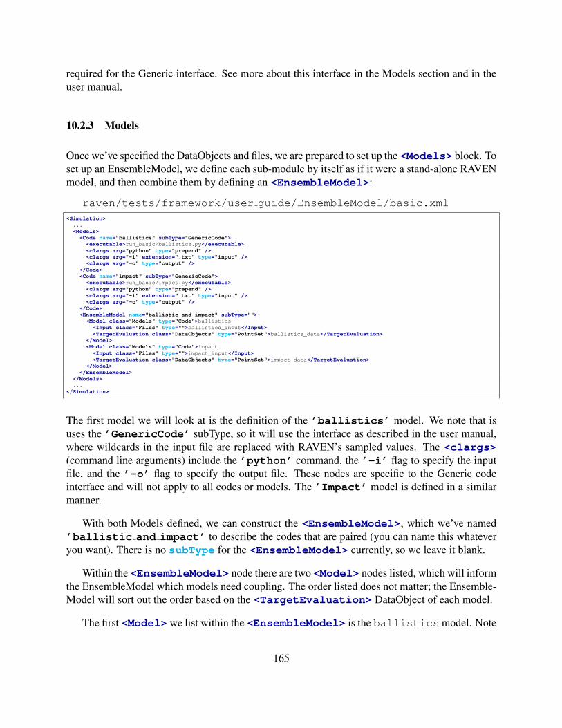
required for the Generic interface. See more about this interface in the Models section and in theuser manual.
10.2.3 Models
Once we’ve specified the DataObjects and files, we are prepared to set up the <Models> block. Toset up an EnsembleModel, we define each sub-module by itself as if it were a stand-alone RAVENmodel, and then combine them by defining an <EnsembleModel>:
raven/tests/framework/user guide/EnsembleModel/basic.xml<Simulation>...<Models>
<Code name="ballistics" subType="GenericCode"><executable>run_basic/ballistics.py</executable><clargs arg="python" type="prepend" /><clargs arg="-i" extension=".txt" type="input" /><clargs arg="-o" type="output" />
</Code><Code name="impact" subType="GenericCode">
<executable>run_basic/impact.py</executable><clargs arg="python" type="prepend" /><clargs arg="-i" extension=".txt" type="input" /><clargs arg="-o" type="output" />
</Code><EnsembleModel name="ballistic_and_impact" subType="">
<Model class="Models" type="Code">ballistics<Input class="Files" type="">ballistics_input</Input><TargetEvaluation class="DataObjects" type="PointSet">ballistics_data</TargetEvaluation>
</Model><Model class="Models" type="Code">impact
<Input class="Files" type="">impact_input</Input><TargetEvaluation class="DataObjects" type="PointSet">impact_data</TargetEvaluation>
</Model></EnsembleModel>
</Models>...
</Simulation>
The first model we will look at is the definition of the ’ballistics’ model. We note that isuses the ’GenericCode’ subType, so it will use the interface as described in the user manual,where wildcards in the input file are replaced with RAVEN’s sampled values. The <clargs>(command line arguments) include the ’python’ command, the ’-i’ flag to specify the inputfile, and the ’-o’ flag to specify the output file. These nodes are specific to the Generic codeinterface and will not apply to all codes or models. The ’Impact’ model is defined in a similarmanner.
With both Models defined, we can construct the <EnsembleModel>, which we’ve named’ballistic and impact’ to describe the codes that are paired (you can name this whateveryou want). There is no subType for the <EnsembleModel> currently, so we leave it blank.
Within the <EnsembleModel> node there are two <Model> nodes listed, which will informthe EnsembleModel which models need coupling. The order listed does not matter; the Ensemble-Model will sort out the order based on the <TargetEvaluation> DataObject of each model.
The first <Model>we list within the <EnsembleModel> is the ballisticsmodel. Note
165

that the class and type are used along with the name to find the right model. Note also the nameof the model goes in the text of the <Model> node, right after the first closing angle bracket. Thesubnodes of the ’ballistics’ model are the <Input>, which points to the input templateinput file we defined in the <Files> block; and the <TargetEvaluation>, which points tothe <PointSet> we defined in the <DataObjects> block. These are critical to allowing theEnsembleModel both to run the ’ballistics’ model correctly, as well as the entire ensemblein a sensible manner.
In general, some models (such as a <ROM> or <ExternalModel>) do not require any filesas inputs. In this case, the <Input> for an input-less model should be a placeholder DataObject,usually with the same input space as the <TargetEvaluation> DataObject, and a placeholderoutput. For more information, see examples running ExternalModels in these guides as well as theuser manual.
After the ’ballistics’ model, we see a similar structure pointing to the ’impact’model. The only differences between this model specification and the ballistics model specifi-catoin are the names of the <Input> file and <TargetEvaluation> DataObject.
With the two models defined, and the EnsembleModel assembled, no more work is required toprepare these two models to run. More complicated systems may require additional nodes in theEnsembleModel; see the user manual for details.
10.2.4 Steps
Finally, to put all the pieces together, we consider the <Steps> node:
raven/tests/framework/user guide/EnsembleModel/basic.xml
<Simulation>...<Steps><MultiRun name="sample">
<Input class="Files" type="">ballistics_input</Input><Input class="Files" type="">impact_input</Input><Model class="Models" type="EnsembleModel">ballistic_and_impact</Model><Sampler class="Samplers" type="Grid">grid</Sampler><Output class="DataObjects" type="PointSet">final_results</Output>
</MultiRun><IOStep name="print">
<Input class="DataObjects" type="PointSet">final_results</Input><Output class="OutStreams" type="Print">results</Output>
</IOStep></Steps>...
</Simulation>
We take two steps in this simulation, one <MultiRun> called ’sample’ to sample the Ensem-bleModel on a grid, and one <IOStep> to print the results. These are constructed just as theywould be with any other model; as far as the <Steps> are concerned, the EnsembleModel is like
166
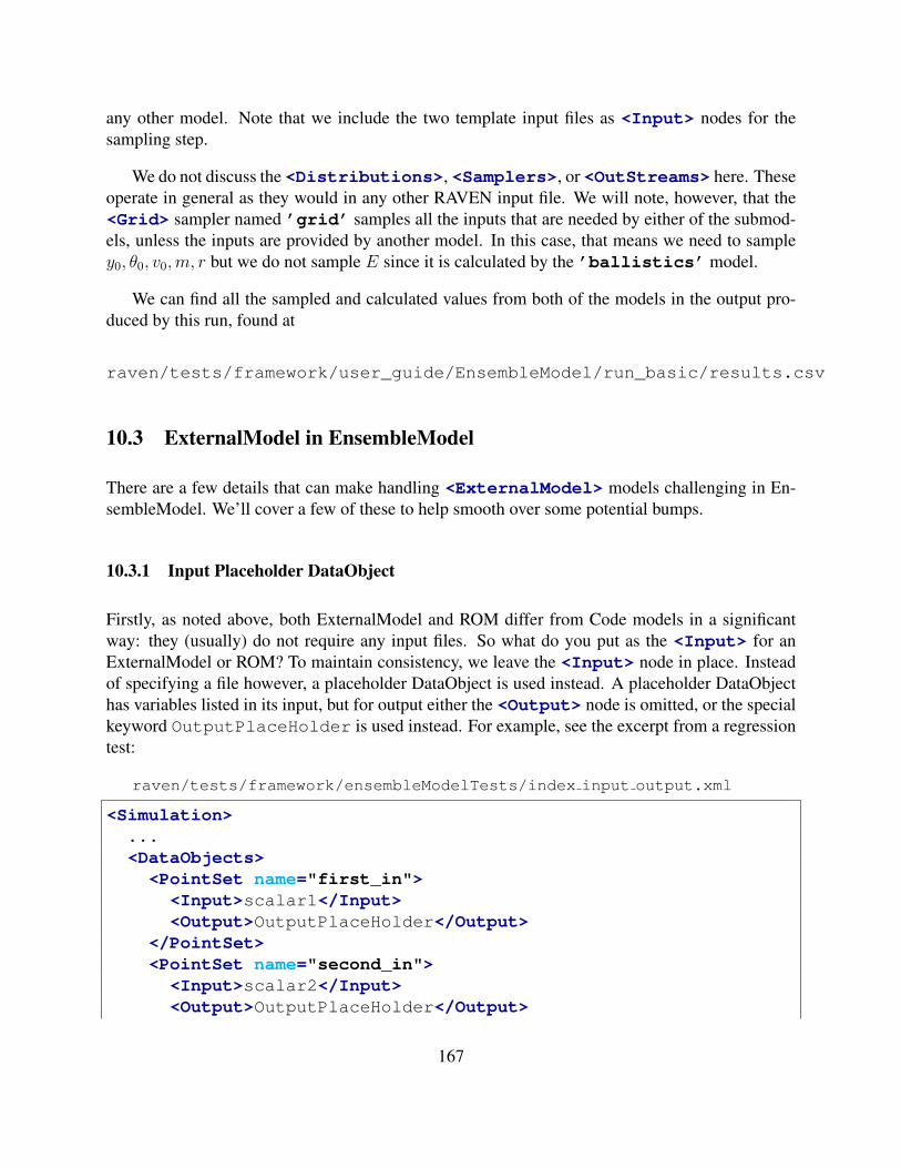
any other model. Note that we include the two template input files as <Input> nodes for thesampling step.
We do not discuss the <Distributions>, <Samplers>, or <OutStreams> here. Theseoperate in general as they would in any other RAVEN input file. We will note, however, that the<Grid> sampler named ’grid’ samples all the inputs that are needed by either of the submod-els, unless the inputs are provided by another model. In this case, that means we need to sampley0, θ0, v0,m, r but we do not sample E since it is calculated by the ’ballistics’ model.
We can find all the sampled and calculated values from both of the models in the output pro-duced by this run, found at
raven/tests/framework/user_guide/EnsembleModel/run_basic/results.csv
10.3 ExternalModel in EnsembleModel
There are a few details that can make handling <ExternalModel> models challenging in En-sembleModel. We’ll cover a few of these to help smooth over some potential bumps.
10.3.1 Input Placeholder DataObject
Firstly, as noted above, both ExternalModel and ROM differ from Code models in a significantway: they (usually) do not require any input files. So what do you put as the <Input> for anExternalModel or ROM? To maintain consistency, we leave the <Input> node in place. Insteadof specifying a file however, a placeholder DataObject is used instead. A placeholder DataObjecthas variables listed in its input, but for output either the <Output> node is omitted, or the specialkeyword OutputPlaceHolder is used instead. For example, see the excerpt from a regressiontest:
raven/tests/framework/ensembleModelTests/index input output.xml
<Simulation>...<DataObjects>
<PointSet name="first_in"><Input>scalar1</Input><Output>OutputPlaceHolder</Output>
</PointSet><PointSet name="second_in">
<Input>scalar2</Input><Output>OutputPlaceHolder</Output>
167
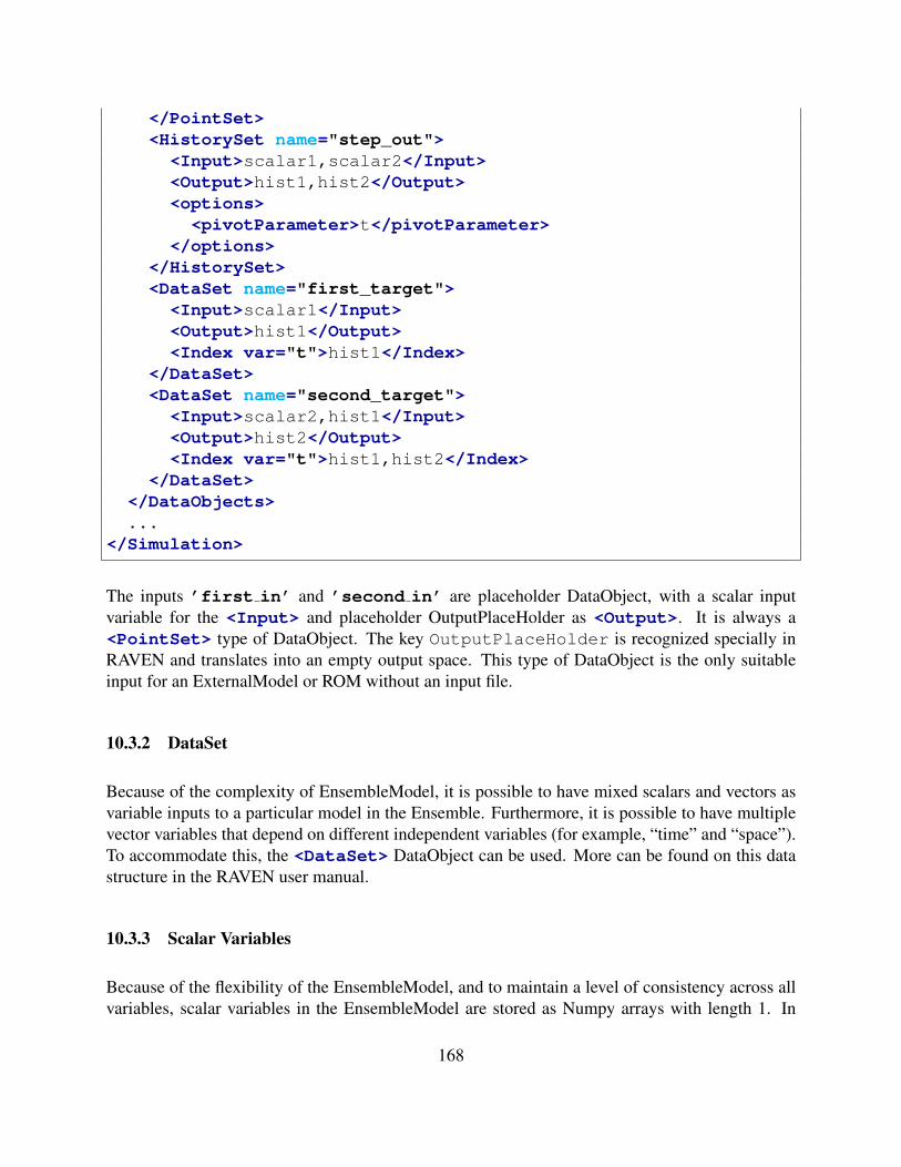
</PointSet><HistorySet name="step_out">
<Input>scalar1,scalar2</Input><Output>hist1,hist2</Output><options><pivotParameter>t</pivotParameter>
</options></HistorySet><DataSet name="first_target">
<Input>scalar1</Input><Output>hist1</Output><Index var="t">hist1</Index>
</DataSet><DataSet name="second_target">
<Input>scalar2,hist1</Input><Output>hist2</Output><Index var="t">hist1,hist2</Index>
</DataSet></DataObjects>...
</Simulation>
The inputs ’first in’ and ’second in’ are placeholder DataObject, with a scalar inputvariable for the <Input> and placeholder OutputPlaceHolder as <Output>. It is always a<PointSet> type of DataObject. The key OutputPlaceHolder is recognized specially inRAVEN and translates into an empty output space. This type of DataObject is the only suitableinput for an ExternalModel or ROM without an input file.
10.3.2 DataSet
Because of the complexity of EnsembleModel, it is possible to have mixed scalars and vectors asvariable inputs to a particular model in the Ensemble. Furthermore, it is possible to have multiplevector variables that depend on different independent variables (for example, “time” and “space”).To accommodate this, the <DataSet> DataObject can be used. More can be found on this datastructure in the RAVEN user manual.
10.3.3 Scalar Variables
Because of the flexibility of the EnsembleModel, and to maintain a level of consistency across allvariables, scalar variables in the EnsembleModel are stored as Numpy arrays with length 1. In
168

general this should be transparent for most operations; however, occasionally it may be requiredto access a scalar variable by accessing it at index 0. For example, see the variable “scalar2” in amodel used in the regression tests for the EnsembleModel:
raven/tests/framework/ensembleModelTests/IndexInputOutput/model2.py
import numpy as np
def run(obj,dct):obj.t #just making sure it's available hereobj.hist2 = obj.hist1 + obj.scalar2[0]
10.3.4 Independent Variables
One feature of ExternalModel is their capacity to take variables exactly as they are from RAVEN,without going through file IO. As a result, EnsembleModel frequently contain models that producepivot-dependent data that can be used as inputs for other models in the Ensemble. Several termsaptly describe these variables on which other variables depend, including “independent variables,”“indexes”, and “pivots”. In general, we refer to them as “indexes”. While the index is often “time”or something similar, it can be any monotonically-increasing variable.
However, when it is stored in RAVEN, the indexes are not stored like other variables, because itis a coordinate axes that supports other variables. This allows RAVEN to do a great many flexibleoperations internally. However, it also means that any time you want to pass an index variable fromone model to an ExternalModel, it can only come attached to another variable that depends on thatinput.
For example, consider two models. In the first model, a path followed by a charged particleis traced out in time. The outputs of the first model are time t, lateral position x, and verticalposition y. The second model calculates the energy of the particle at each point in time; however,the second model is written such that it does not require any specific time values (it just reads themfrom the input).
To run these two models in Ensemble configuration, <TargetEvaluation> DataObject ofthe second model must request one of the time-dependent variables from the first model, x or y.If t is directly requested, it will not be made available in the second ExternalModel. Additionally,in the <Model> definition, all variables (dependent or index) should be listed. In this example,when defining the model, t should be listed as well as x in the <variables> node in the second<Model> definition.
For an example of time dependent data passing, consider the regression test example at
169

raven/tests/framework/ensembleModelTests/index_intput_output.xml
170

Appendices
A Document Version Information
tag number 23-192-gb3087a02462a386fc1da99a1d77afb73e2ad19e7e47fd5a72 Paul TalbotTue, 22 May 2018 12:47:08 -0600
171

References
[1] “Neams: The nuclear energy advanced modeling and simulation program,” Tech. Rep.ANL/NE-13/5.
[2] “Light water reactor sustainability program integrated program plan,” Tech. Rep. INL-EXT-11-23452, April 2013.
[3] R.-D. development team, “Relap5/mod3.3 code manual,” tech. rep., Idaho National Labora-tory, October 2015.
[4] C. Rabiti, A. Alfonsi, J. Cogliati, D. Mandelli, R. Kinoshita, and S. Sen, “Raven user manual,”tech. rep., Idaho National Laboratory, 2015.
[5] A. Alfonsi, C. Rabiti, D. Mandelli, J. Cogliati, and B. Kinoshita, “Raven as a tool for dynamicprobabilistic risk assessment: Software overview,” in Proceedings of International Confer-ence of mathematics and Computational Methods Applied to Nuclear Science and Engineering(M&C 2013), Sun Valley (Idaho), pp. 1247–1261, 2013.
[6] A. Alfonsi, C. Rabiti, D. Mandelli, J. Cogliati, B. Kinoshita, and A. Naviglio, “Dynamic eventtree analysis through raven,” in Proceedings of ANS PSA 2013 International Topical Meetingon Probabilistic Safety Assessment and Analysis, Columbia (South Carolina), 2013.
[7] C. Rabiti, A. Alfonsi, D. Mandelli, J. Cogliati, and R. Kinoshita, “Deployment and overviewof raven capabilities for a probabilistic risk assessment demo for a pwr station blackout,” Tech.Rep. INL/EXT-13-29510, Idaho National Laboratory (INL), 2013.
[8] A. Alfonsi, C. Rabiti, D. Mandelli, J. Cogliati, and B. Kinoshita, “Raven and dynamic prob-abilistic risk assessment: Software overview,” in Proceedings of ESREL European Safety andReliability Conference (ESREL 2014), Wrocklaw (Poland), 2014.
[9] D. Anders, R. Berry, D. Gaston, R. Martineau, J. Peterson, H. Zhang, H. Zhao, and L. Zou,“Relap-7 level 2 milestone report: Demonstration of a steady state single phase pwr simulationwith relap-7,” Tech. Rep. INL/EXT-12-25924, Idaho National Laboratory (INL), 2012.
172

v1.28