Rational Inattention, Optimal Consideration Sets and

Stochastic Choice∗

Andrew Caplin†, Mark Dean‡, and John Leahy§

January 2018

Abstract

We unite two basic approaches to modelling limited attention in choice by show-

ing that the rational inattention model implies the formation of consideration sets —

only a subset of the available alternatives will be considered for choice. We provide

necessary and suffi cient conditions for rationally inattentive behavior which allow the

identification of consideration sets. In simple settings, chosen options are those that

are best on a stand-alone basis. In richer settings, the consideration set can only be

identified holistically. In addition to payoffs, prior beliefs impact consideration sets.

Simple linear equations identify all priors consistent with each possible consideration

set.

1 Introduction

Attention is a scarce resource. The impact of attentional limits has been identified in many

important economic settings,1 leading to widespread efforts to model the effect of such con-∗We thank Dirk Bergemann, Henrique de Oliveira, Xavier Gabaix, Sen Geng, Andrei Gomberg, Daniel

Martin, Filip Matejka, Alisdair McKay, Stephen Morris, Dan Silverman and Michael Woodford for theirconstructive contributions. This paper develops some of the concepts of Caplin and Dean [2013] and subsumesthose parts of that paper that are common.†Center for Experimental Social Science and Department of Economics, New York University. Email:

andrew.caplin@nyu.edu‡Department of Economics, Columbia University. Email: mark.dean@columbia.edu§Department of Economics and Gerald R. Ford School of Public Policy, University of Michigan and

NBER. Email: jvleahy@umich.edu1For example, shoppers may buy unnecessarily expensive products due to their failure to notice whether

or not sales tax is included in stated prices (Chetty et al. [2009]). Buyers of second-hand cars focus their

1

straints.

One key implication of limited attention is that a decision maker may consider only a

subset of the available alternatives, ignoring all others. The concept of ‘consideration sets’has

a long history in the marketing literature, which extensively demonstrates their importance.2

More recently, economists have begun to understand the importance of consideration sets

for many areas of study - including revealed preference analysis, the price setting behavior

of firms, and demand estimation.3

A second implication of attentional constraints is that choice may be stochastic: a de-

cision maker may make different choices in seemingly identical situations. Random choice

has been demonstrated in a wide variety of experimental settings.4 The relationship be-

tween stochasticity and attention constrained choice has been emphasized by the ‘rational

inattention’approach of Sims [2003], in which the decision maker (DM) chooses information

optimally given their decision problem, with costs based on the Shannon mutual information

between prior and posterior beliefs (henceforth the Shannon model).

In this paper we unite these two approaches, and present a theory of optimal considera-

tion set formation based on rational inattention. We show that an implication of the Shannon

model in discrete choice settings is that, typically, many options will never be chosen, and

will receive no consideration.5 The set of considered alternatives arises endogenously, based

on prior beliefs and attention costs. Moreover, the same parameters determine a pattern

of stochastic choice ‘mistakes’amongst considered alternatives, in line with experimental

findings.6 Unlike current models, our approach therefore provides a tractable, parsimonious

model of both endogenous consideration set formation and choice mistakes within the con-

sideration set.

In order to develop our model, we introduce a set of necessary and suffi cient first order

conditions for the Shannon model. These build on the necessary conditions of Matejka and

McKay [2015] (henceforth MM), who characterize the pattern of stochastic choice implied

by the Shannon model amongst alternatives which are chosen with positive probability. We

introduce a set of easy-to-check inequality constraints which determine the set of chosen

attention on the leftmost digit of the odometer (Lacetera et al. [2012]). Purchasers limit their attention toa relatively small number of websites when buying over the internet (Santos et al. [2012]).

2For example Hoyer [1984], Hauser and Wernerfelt [1990] and Roberts and Lattin [1991].3See for example Ching et al. [2009], Eliaz and Spiegler [2011], Caplin et al. [2011], Masatlioglu et al.

[2012], De Clippel et al. [2014], Manzini and Mariotti [2014].4See for example Mosteller and Nogee [1951], Reutskaja et al. [2011] and Agranov and Ortoleva [2017a].5In a manner we make precise in Section 3. See also Jung et al. [2015].6See for example Geng [2016]

2

actions, and so also the set of actions which are never chosen (see also Stevens [2014]).

These conditions are crucial to the solution of the Shannon model in any application - not

only those we consider in this paper: generally not all actions with be taken at the optimum,

and there will be many suboptimal patterns of behavior which satisfy MM’s conditions.

Using our necessary and suffi cient conditions, we consider behavior in three variants

of the standard consumer problem. In each case, the consumer must choose one of a set of

available alternatives. The value of each alternative is ex ante uncertain, but that uncertainty

can be reduced by allocating attention and incurring the associated subjective costs. The

three decision making environments vary in the assumed correlation structure between the

valuations of different alternatives.

In our first application the consumer must choose between a number of alternatives, one

of which is of high quality and the remainder of which are of low quality. The identity of the

high quality alternative is unknown ex ante, but can be learned by the consumer. In this

setting, the Shannon model implies that consideration sets are determined by a threshold

strategy: consumers will consider only alternatives which have a prior probability of being

high quality which is above an endogenously determined threshold. Alternatives below this

threshold will never be chosen even though there is a chance that this set includes the high

quality good. Amongst considered alternatives, attention is allocated in such a way that

ex post all choices are identical: the probability of any alternative being of high quality

conditional on being chosen is the same, regardless of prior belief.

In our second environment we assume that the valuation of different alternatives is in-

dependent. In this setting, consideration set formation is again driven by a cutoff strategy.

However, the ranking of alternatives is now determined by the expectation of a convex trans-

formation of the payoffs. This transformation reflects the gains to information acquisition:

the ability to take an action when its payoff is relatively high and avoid it when its payoff is

low. Given this convex transformation, the composition of consideration sets can change in

rich and non-monotonic ways as information costs change. We provide an example in which

the consumer must choose either a safe alternative, the value of which is known ex ante, or

one of a set of risky alternatives, the value of which must be learned. The safe alternative

only appears in the consideration set at very high information costs - when it allows the

consumer to be uninformed, or very low information costs - when it is chosen if all the risky

alternatives turn out to be of low quality. For information costs in an intermediate range,

the consideration set consists only of the risky alternatives. We further demonstrate that, if

prizes are denominated in monetary terms, the make up of the consideration set is jointly

determined by the information costs and risk aversion of the consumer: risky alternatives

3

will only be used if the consumer has low attention costs or low risk aversion.

In our third environment, we look at the most general case of arbitrary correlation be-

tween the valuations of different alternatives - for example of the type that might occur in

the choice of financial products. In this case, no simple cutoff rule determines the consid-

eration set. This is due to the fact that even risk neutral consumers have a hedging motive

in this environment: the value of an action depends on its payoff relative to other actions

in each state. Given this hedging motive, the consideration set will depend on the complete

range of available alternatives. We show that our conditions imply a simple test of whether

a new alternative will be considered if it is introduced to an existing market, and identify

the lowest cost way of ensuring such an alternative will be chosen.

An essential feature of rational inattention is that choice depends on prior beliefs. In our

model this means that, even if we fix the payoffs to all available actions, the consideration

set depends on the prior. We show that our necessary and suffi cient conditions produce a

simple system of linear equations that can be used to identify all priors consistent with each

possible consideration set.

Section 5 discusses the relationship of our work to existing models of consideration set

formation. Recent papers have typically taken consideration sets as primitives for the con-

sumer (in the same way that preferences are primitives), therefore sidestepping the issue

of how the set of considered items is determined. These papers then focus on identifying

the consideration set from choice behavior (Masatlioglu et al. [2012], Manzini and Mariotti

[2014]) or on understanding firm behavior conditional on such sets (Eliaz and Spiegler [2011]).

Moreover, these models assume that decision makers deterministically maximize preferences

on the consideration set.7 Yet recent evidence (e.g. Geng [2016]) shows that choice may be

stochastic even amongst considered alternatives. As with Manzini and Mariotti [2014], our

work provides a link between the study of consideration sets and the recent literature aimed

at understanding stochastic choice data (e.g. Agranov and Ortoleva [2017b], Manzini and

Mariotti [2016], Apesteguia et al. [2017]). An earlier literature in marketing discussed models

of endogenous consideration set formation (e.g. Hauser and Wernerfelt [1990], Roberts and

Lattin [1991]). However, these have typically had to focus on very stylized cases for the sake

of tractability: sequential choice of information in more complex settings quickly become

intractable (see for example Gabaix et al. [2006]).

Section 2 introduces the Shannon model and our necessary and suffi cient conditions.

Section 3 describes our three applications to consumer search. Section 4 introduces the

7Though see for example Goeree [2008].

4

linear equations that allow priors to be partitioned according to the rationally inattentive

consideration set. Section 5 reviews the existing literature, and section 6 concludes.

2 The Shannon Model

We consider a consumer who faces a decision problem which consists of a number of different

alternatives from which they must make a choice. The value of each alternative is deter-

mined by the underlying state of the world. Prior to choice, the decision maker can receive

information about the state of the world in the form of an information structure, which

consists of a set of signals, and a stochastic mapping between the true state of the world and

these signals. More accurate signals will lead to better choices, but are more costly, with

costs based on the Shannon mutual information between prior and posterior beliefs. This is

the model of ‘rational inattention’introduced by Sims [2003].

2.1 The Decision Problem

There are finitely many states of the world Ω, with ω ∈ Ω denoting a generic state. An

action is a mapping from states of the world to utilities. We use A to denote the set of

actions, and u : A × Ω → R to identify the utility of each action in each state. A decisionproblem (µ,A) consists of a prior distribution µ ∈ ∆(Ω) over these states of the world and

a finite subset of options A ⊆ A from which the decision maker must choose.

It is well known that one can solve the Shannon model by treating the decision problem

as one of choosing the probability of each action in each state, rather than the choice of

information structure (see for example MM Corollary 1). Thus, given the decision problem

(µ,A), the decision maker chooses the probability of receiving option a ∈ A in each state

ω: i.e., for a given A they choose a P : Ω → ∆(A), with P (a|ω) denoting the probability

of choosing action a in state ω, and P the set of all such state dependent stochastic choicefunctions.

The value of P ∈ P is given by the expected value of the actions chosen, minus informa-tion costs. These costs are based on the Shannon mutual information between states and

actions - i.e. the difference between the expected entropy of the conditional and uncondi-

tional choice distributions.8 Intuitively, having choice distributions which vary a lot with

8The entropy of a distribution p on Ω is given by −∑

ω∈Ω p(ω) ln p(ω). Broadly speaking a high degreeof entropy means that there is a lot of uncertainty.

5

the state requires costly information. MM Corollary 1 shows that the optimization problem

of a consumer facing a decision problem (µ,A) can be written as follows:

The Decision Problem Choose P ∈ P in order to maximize

∑ω∈Ω

µ(ω)

(∑a∈A

P (a|ω)u(a, ω)

)(1)

−λ[∑ω∈Ω

µ(ω)

(∑a∈A

P (a|ω) lnP (a|ω)

)−∑a∈A

P (a) lnP (a)

]

where P (a) =∑

ω∈Ω µ(ω)P (a|ω).

The first term is the expected payoffdue to the set of state contingent choice probabilities.

The second term is the cost of information which is equal to the mutual information between

states and actions multiplied by the parameter λ, which describes the marginal cost of

information.

2.2 Necessary and Suffi cient Conditions

MM show that the optimal policy must satisfy the following condition for all actions a ∈ Asuch that P (a) > 0:

P (a|ω) =P (a)z(a, ω)∑b∈A P (b)z(b, ω)

(2)

where z(a, ω) ≡ exp(u(a, ω)/λ). This condition states that the optimal policy “twists”the

choice probabilities towards states in which the payoffs are high.

While the conditions (2) are necessary, they are not suffi cient. For example, for any

option a, the stochastic choice function P (a|ω) = 1 for all ω satisfies these conditions. This

is not surprising since this is the optimal policy when only option a is available and the

necessary conditions depend on the choice set only in the sense that all of the choices in the

sum in the denominator must be available.

The key limitation of these conditions is that, while they determine stochastic choice

amongst alternatives which are chosen with positive probability, they do not identify which

alternatives belong to this set. Doing so is important because, as we shall see, generally

there will be many unchosen actions in a given decision problem. We will describe the set

of actions which are chosen with positive probability as the consideration set, and for every

6

P ∈ P we will use B(P ) to denote the associated consideration set - i.e.

B(P ) = a ∈ A|P (a) > 0 .

Using this definition we can state the central proposition of the paper, which provides

necessary and suffi cient conditions for P to be a solution to the rational inattention problem.

This only requires solving for the unconditional probabilities of the options, P (a), as the state

contingent choice probabilities, P (a|ω), are completely determined by these unconditional

probabilities and the MM conditions in equation (2).

Proposition 1 The policy P ∈ P is optimal if and only if:

∑ω∈Ω

z(a, ω)µ(ω)∑b∈A P (b)z(b, ω)

≤ 1, (3)

for all a ∈ A, with equality if a ∈ B(P ); and if for all such actions and states ω, P (a|ω)

satisfies equation (2).

Proof. First, note that we can use the MM conditions for P (a|ω) to rewrite the objective

function from equation (1) in terms of the unconditional probabilities P (a),∑ω∈Ω

∑a∈A

µ(ω)P (a|ω) (u(a, ω)− λ lnP (a|ω)) + λ∑a∈A

P (a) lnP (a)

=∑ω∈Ω

∑a∈A

µ(ω)P (a|ω)

(u(a, ω)− λ ln

[P (a)z(a, ω)∑b∈A P (b)z(b, ω)

])+ λ

∑a∈A

P (a) lnP (a).

We can rewrite the term in parentheses as

u(a, ω)− λ ln

[P (a)z(a, ω)∑b∈A P (b)z(b, ω)

]= u(a, ω)− λ lnP (a)− λ ln z(a, ω) + λ ln

∑b∈A

P (b)z(b, ω)

= −λ[

lnP (a)− ln∑b∈A

P (b)z(b, ω)

].

Substituting this back in to the objective function gives

−λ∑ω∈Ω

∑a∈A

µ(ω)P (a|ω) lnP (a)+λ∑ω∈Ω

∑a∈A

µ(ω)P (a|ω) ln∑b∈A

P (b)z(b, ω)+λ∑a∈A

P (a) lnP (a).

7

The first and last terms cancel out, and the logarithm in the middle term is not a function

of a, leaving ∑ω∈Ω

λ ln

(∑b∈A

P (b)z(b, ω)

)µ(ω).

This new objective is concave in P (b) and the constraints on P (b) are linear. Hence the

Kuhn-Tucker conditions are necessary and suffi cient. We can write a Lagrangian for the

problem:

maxP∈P

∑ω∈Ω

λ ln

(∑b∈A

P (b)z(b, ω)

)µ(ω)− ϕ

(∑b∈A

P (b)− 1

)+∑b∈A

ξbP (b) (4)

where ϕ is the Lagrangian multiplier on the constraint that the unconditional probabilities

P (b) must sum to 1, and ξb is the multiplier on the non-negativity constraint for P (b).

The associated first order condition with respect to P (a) is

λ∑ω∈Ω

z(a, ω)(∑b∈A P (b)z(b, ω)

)µ(ω)− ϕ+ ξa = 0.

The complementary slackness condition is ξaP (a) = 0 and ξa ≥ 0.

If P (a) > 0 then ∑ω∈Ω

λz(a, ω)∑

b∈A P (b)z(b, ω)µ(ω) = −ϕ.

Multiplying by P (a) and summing over a gives

λ = −ϕ.

So if P (a) > 0 ∑ω∈Ω

z(a, ω)∑b∈A P (b)z(b, ω)

µ(ω) = 1.

If P (a) = 0 then ξa ≥ 0

∑ω∈Ω

z(a, ω)∑b∈A P (b)z(b, ω)

µ(ω) = 1− ξa

λ≤ 1.

These are the necessary and suffi cient conditions for an optimum.

We can gain some intuition for these conditions by considering the Blahut-Arimoto algo-

rithm (see Cover and Thomas [2012]). The algorithm proceeds by first choosing P (a|ω) given

8

a guess for the P (a) and then generating a new P (a) given P (a|ω). Since it can be shown

that the objective function in equation (1) rises with each step, the algorithm converges.

The solution to the first step is MM’s necessary conditions

Pn+1(a|ω) =Pn(a)z(a, ω)∑b∈A Pn(b)z(b, ω)

.

The solution to the second step invokes Bayes rule: Pn+1(a) =∑

ω∈Ω Pn+1(a|ω)µ(ω). Putting

these together,

Pn+1(a) =

(∑ω∈Ω

z(a, ω)µ(ω)∑b∈A Pn(b)z(b, ω)

)Pn(a).

The term in brackets is the left side of (3) and determines if P (a) rises or falls. The algorithm

can have one of two steady states. Either P (a) > 0 and the term in brackets is equal to one,

a case that includes P (a) = 1, or the term in brackets is less than one and P (a) = 0 and

can fall no further. (2) represents a twist in state dependent choice in the direction of the

high payoff states. (3) ensures that these twists average out to one. If they don’t then the

probability of an action needs to be raised or lowered accordingly.

The condition in Proposition 1 resembles, but is stronger than that of Corollary 2 in MM,

which states that, if P ∈ P is optimal, then (3) must hold with equality for a ∈ B(P ). The

difference is that our Proposition 1 provides necessary and suffi cient conditions for a policy

to be optimal, because it provides conditions on both chosen and unchosen acts. Generally

there will be many P ∈ P which satisfy the equality condition of MM Corollary 2, yet are

not optimal, meaning that on its own this condition is of limited practical use in solving the

Shannon model. We illustrate the importance of the suffi ciency portion of Proposition 1 in

section 3.1.3.

2.3 A Posterior-Based Approach

It is insightful to recast the solution of the Shannon model in terms of the implied posterior

beliefs. Note any set of stochastic choices P ∈ P imply posterior belief γa ∈ ∆(Ω) at any

a ∈ B(P ). By Bayes’rule,

γa(ω) =P (a|ω)µ(ω)

P (a),

where γa(ω) is the probability of state ω given the choice of a. There is a one-to-one mapping

between the set of state dependent stochastic choices P ∈ P and the set of unconditionalchoice probabilities and posterior beliefs P (a)a∈A, γaa∈B(P ). We can rewrite the nec-

9

essary and suffi cient conditions of Proposition 1 in terms of these objects.

Proposition 2 Consider the choice problem (A, µ) and policy P (a)a∈A and γaa∈B(P ).

The policy is optimal if and only if∑

a∈A P (a)γ(ω) = µ(ω) and

1. Invariant Likelihood Ratio (ILR) Equations for Chosen Options: given a, b ∈B(P ), and ω ∈ Ω,

γa(ω)

z(a, ω)=

γb(ω)

z(b, ω).

2. Likelihood Ratio Inequalities for Unchosen Options: given a ∈ B(P ) and c ∈A\B(P ), ∑

ω∈Ω

[γa(ω)

z(a, ω)

]z(c, ω) ≤ 1. (5)

Proof. It follows immediately from (2) that, for a ∈ B(P )

γa(ω)

z(a, ω)=

µ(ω)∑b∈A P (b)z(b, ω)

.

The necessary and suffi cient conditions (3) become

γa(ω)

z(a, ω)=

γb(ω)

z(b, ω)(6)

when options a and b are chosen and

∑ω∈Ω

z(c, ω)γa(ω)

z(a, ω)≤ 1 (7)

when option a is chosen and option c is not.

The name ‘Invariant Likelihood Ratio’stems from the obvious rewriting of the equality

conditionγa(ω)

γb(ω)=z(a, ω)

z(b, ω)

which shows that the ratio of the posterior probability of a given state following the choice

of action a and b depends only on the (normalized) relative payoffs of the two actions in

that state, not prior beliefs, the payoffs of these actions in other states or the payoff of other

actions.9

9Note that, for any a ∈ B(A) and ω ∈ Ω the Shannon mode impliesl γa(ω) > 0 so this ratio is alwayswell defined.

10

Intuition for the ILR condition can be gleaned from the geometric approach introduced

in Caplin and Dean [2013] and discussed further in section 3.3.1. This associates with the

posterior γa a ‘net utility’

N(γa) =∑ω∈Ω

[γa(ω)u(a, ω)− λγa(ω) ln γa(ω)]

which captures both the benefits and costs of using such a posterior when choosing action

a. As demonstrated in section 3.3.1, a necessary condition for optimality is that the slope of

the net utility function is the same for each chosen act at its associated posterior. Consider a

simple case in which there are two states ω1 and ω2, and two actions a and b. The posterior

γa can be defined solely through γa(ω1), as γa(ω2) = 1− γ(ω1). The slope of the net utility

function is therefore given by

∂N(γa)

∂γa(ω1)= u(a, ω1)− u(a, ω2)− λ [ln γa(ω1)− ln γa(ω2)] ,

and the condition that the net utility functions have the same slope implies

[u(a, ω1)− λ ln γa(ω1)]− [u(a, ω2)− λ ln γa(ω2)]

= [u(b, ω1)− λ ln γb(ω1)]− [u(b, ω2)− λ ln γb(ω2)].

While there are, in principle, many ways for this equation to be satisfied, one suffi cient

condition is for it to hold ‘state by state’,

u(a, ω)− λ ln γa(ω) = u(b, ω)− λ ln γb(ω) for all ω ∈ Ω,

which is precisely the ILR condition. Proposition 2 establishes that this is indeed the correct

solution.

The ILR condition can also be thought of as capturing a ‘constant returns to scale’feature

of the Shannon model. Consider changing a decision problem by ‘splitting’a particular state

in two yet keeping the underlying payoff structure, so all actions pay off identically in the two

new states. In principal this could make it harder or easier for the DM to learn about these

states. What the ILR condition captures is that the Shannon model predicts that behavior is

invariant to such changes: only the payoffs in each state matter. This property, which Caplin

et al. [2017] formalize in an axiom called ‘Invariance Under Compression’, is what identifies

the Shannon model within a broader class of information cost functions. For example, costs

based on Tsallis entropy (Tsallis [1988]) could lead decision makers to become more or less

11

accurate in response to the splitting of states, depending on the parameterization, thus

violating the ILR condition (see Caplin et al. [2017]).

2.4 Uniqueness

Given our interest in consideration sets, it is of value later to impose conditions for uniqueness

of the optimal strategy. These conditions imply that the optimal consideration set B(P ) is

also unique.

Remark 1 Caplin and Dean [2013], Theorem 2, establishes that affi ne independence of the

normalized payoff vectors z(a) ∈ RΩ|a ∈ A, where z(a, ω) ≡ exp(u(a, ω)/λ), ensures

uniqueness of the optimal strategy. Since linear independence implies affi ne independence, it

too is suffi cient.

3 Endogenous Consideration Set Formation

The necessary and suffi cient conditions of Proposition 1 are key to the identification of

optimal choices, something that is not possible with the MM solution alone. They also

highlight a particular feature of such solutions: the available actions can be divided into a

consideration set of alternatives which are chosen with positive probability in every state

of the world, and an excluded set of alternatives which are never chosen in any state. This

provides a link between the Shannon model and models of choice with consideration sets

which have long been popular in the marketing literature (see for example Hoyer [1984],

Hauser and Wernerfelt [1990] and Roberts and Lattin [1991]).

In this section we explore this link further by applying the Shannon model to three

variants of the consumer problem, and characterizing the resulting consideration sets in each

case. We interpret the set A as representing the set of goods for sale, one of which the

consumer will end up buying. The states of the world relate to the quality of each of the

various goods.

The necessary and suffi cient conditions are non-linear and closed form solutions are not

generally available. The three variants of the consumer problem we consider differ in their

complexity. The first we can solve in closed form. In this case, the consumer knows that

exactly one of the available goods is of high quality, while the rest are of low quality. While

12

somewhat stylized as a consumer problem, this setting allows for a particularly clean under-

standing of the consideration set resulting from the Shannon model. In the second case, we

consider the ‘classic’consumer problem in which the valuation of each alternative is drawn

from an independent (but not necessarily identical) distribution. In this case we introduce a

statistic that determines whether an action is or is not in the consideration set. Finally we

discuss the case in which the valuation of different goods may be correlated.

In each case we interpret B(P ) as the consideration set arising from the resulting choice

behavior. In the standard formulation of the consideration set model, items outside that set

are neither chosen nor ‘considered’as candidates for choice (see for example Masatlioglu et al.

[2012] and Manzini and Mariotti [2014]). Hauser and Wernerfelt [1990] state “The basic idea

is that when choosing to make a purchase, consumers use at least a two-stage process. That

is, consumers faced with a large number of brands use a simple heuristic to screen the brands

to a relevant set called the consideration set”(p 393). There are many possible reasons for

this lack of consideration,10 including a lack of awareness of some alternatives or an attempt

to save on cognitive costs. Our model fits best with the latter interpretation: effectively

the DM first decides which alternatives they are going to choose from, based on payoffs

and prior beliefs, then tailors their information gathering to selecting the best option from

within that set. In some cases this means that nothing is learned about the goods outside

the consideration set, so posterior beliefs about the quality of such goods are the same as

prior beliefs. This is true in our model in the case in which valuations of different goods are

independent (Consumer Problem 2). When valuations are not independent, learning about

the quality of items in the consideration set can also lead the DM to update their beliefs about

items outside it (as in Consumer Problem 3).11 However, any learning about the value of

alternatives outside of B(P ) is incidental in that the DM would gather the same information

if these items were not available: for any a ∈ A/B(P ) and choice set A/a the DM will

choose to acquire the same information as they would when faced with set A. This follows

immediately from Proposition 1 and the one-to-one relationship between stochastic choice

and chosen information structure. This property is similar to the identifying assumption of

Masatlioglu et al. [2012], who assume that if an alternative is not in the consideration set,

then its removal from the choice set will not affect the consideration set. This is also true of

the set B(P ) in the Shannon model.

An immediate corollary is that, relative to the chosen information structure, there exists

10Hauser and Wernerfelt [1990] also state that “Empirically, quite a few definitions of evoked sets, relevantsets, and consideration sets have been used”(p.393).11In Consumer Problem 1 nothing is learned about the value of options outside the consideration set

despite the fact that valuations are not independent.

13

none which conveys the same information about the value of actions inside B(P ) but is

less informative about the value of actions outside B(P ) in the Blackwell sense. Such an

information structure would be less informative overall, and so demand lower information

costs, but would provide the same gross payoffs, contradicting the optimality of the chosen

information structure.

3.1 Consumer Problem 1: Finding the Good Alternative

We begin with a simple yet canonical case. The consumer is faced with a range of possible

goods identified as a set A = a1, .., aM. One of these options is good. The others are bad.The utilities of the good and bad options are uG and uB respectively, with uG > uB. The

DM has a prior on which of the available options is good. We define the state space to be

the same as the action space, Ω = A, with the interpretation that state ωi is the state in

which option i is of high quality and all others are of low quality. Thus

u(ai, ωj) = uG if i = j

= uB otherwise.

µ(ωi) is therefore the prior probability that option ai yields the good prize. Without loss of

generality, we order states according to perceived likelihood,

µi = µ(ωi) ≥ µ(ωi+1) = µi+1.

The DM can expend attentional effort to gain a better understanding of where the prize

is located. The cost of improved understanding is defined by the Shannon model with

parameter λ > 0.

3.1.1 Characterization

To simplify characterization of the optimal strategy, it is convenient to transform parameters

by defining x, δ > 0 as below,

z(ai, ωj) =

exp

(uGλ

)≡ x(1 + δ) if i = j;

exp(uBλ

)≡ x if i 6= j.

The optimal policy will depends on δ, but not on x. Increases in the utility differential

uG− uB and reductions in learning costs both affect the optimal policy through increases in

14

δ.

Substituting these payoffs in to the necessary and suffi cient conditions (3) for some action

ai ∈ B(P ) yields

δµi1 + δP (ai)

+∑

aj∈B(P )

µj(1 + δP (aj))

+∑

ak∈A\B(P )

µk = 1

Since the latter two terms on the left-hand side are the same for all chosen actions, it follows

that the optimal policy equalizes the first term:

µi1 + δP (ai)

across ai ∈ B(P ). This equality has two implications. First, actions that are more likely to

be optimal are more than proportionately more likely to be taken:

µi > µj =⇒ P (ai)/P (aj) > µi/µj.

Second, if the firstK actions are taken with positive probability then the first order condition

for the Kth action and the equality of the µi1+δP (ai)

together imply,

(δ +K)µK

1 + δP (aK)=

K∑k=1

µk,

which requires µK to be greater than 1K+δ

∑Kk=1 µk. Suppose, for example, δ = 1, then

µ2/(µ1+µ2)must be greater than 1/3 if the first two actions are to be considered, µ5/(∑5

1 µa)

must be greater than 1/6 if the first five actions are to be considered, and so on.

Following up on these observations, Theorem 1 provides a complete characterization of

the optimal strategy for this problem according to the Shannon Model. The proof is in the

appendix.

Theorem 1 If µM > 1M+δ

define K = M . If µM < 1M+δ

, then define K < M as the unique

integer such that,

µK >

∑Kk=1 µ(ωk)

K + δ≥ µK+1. (8)

Then the optimal attention strategy involves,

P (ai) =µ(ωi)(K + δ)−

∑Kk=1 µ(ωk)

δ∑K

k=1 µ(ωk)> 0 (9)

15

for i ≤ K, with P (ai) = 0 for i > K. Furthermore the posteriors associated with all chosen

options ai ≤ K take the same form,

γi(ωj) =

(1+δ)

∑Kk=1 µ(ωk)

K+δfor i = j;∑K

k=1 µ(ωk)

K+δfor i 6= j and j ≤ K

µ(ωj) for j > K.

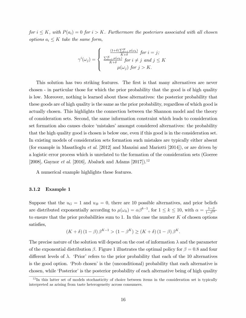
This solution has two striking features. The first is that many alternatives are never

chosen - in particular those for which the prior probability that the good is of high quality

is low. Moreover, nothing is learned about these alternatives: the posterior probability that

these goods are of high quality is the same as the prior probability, regardless of which good is

actually chosen. This highlights the connection between the Shannon model and the theory

of consideration sets. Second, the same information constraint which leads to consideration

set formation also causes choice ‘mistakes’amongst considered alternatives: the probability

that the high quality good is chosen is below one, even if this good is in the consideration set.

In existing models of consideration sets formation such mistakes are typically either absent

(for example in Masatlioglu et al. [2012] and Manzini and Mariotti [2014]), or are driven by

a logistic error process which is unrelated to the formation of the consideration sets (Goeree

[2008], Gaynor et al. [2016], Abaluck and Adams [2017]).12

A numerical example highlights these features.

3.1.2 Example 1

Suppose that the uG = 1 and uB = 0, there are 10 possible alternatives, and prior beliefs

are distributed exponentially according to µ(ωk) = αβk−1, for 1 ≤ k ≤ 10, with α = 1−β1−β10

to ensure that the prior probabilities sum to 1. In this case the number K of chosen options

satisfies,

(K + δ) (1− β) βK−1 > (1− βK) ≥ (K + δ) (1− β) βK .

The precise nature of the solution will depend on the cost of information λ and the parameter

of the exponential distribution β. Figure 1 illustrates the optimal policy for β = 0.8 and four

different levels of λ. ‘Prior’refers to the prior probability that each of the 10 alternatives

is the good option. ‘Prob chosen’is the (unconditional) probability that each alternative is

chosen, while ‘Posterior’is the posterior probability of each alternative being of high quality

12In this latter set of models stochasticity of choice between items in the consideration set is typicallyinterpreted as arising from taste heterogeneity across consumers.

16

conditional on it being chosen.

Figure 1: Optimal Behavior in Example 1

Figure 1 highlights the key features of the optimal policy according to the Shannon model

in this setting. Looking first at the top left hand panel (λ = 1) we see that there is a distinct

‘consideration set’of three items which are chosen with positive probability. None of the

other alternatives are ever chosen. However, even within the consideration set, the subject

makes ‘mistakes’- for each of the chosen alternatives, the probability of it in fact being high

quality is about 31%. Strikingly, this figure is exactly the same for all chosen alternatives:

despite the fact they had different prior probabilities of being high quality, the decision maker

learns exactly enough to make them all identical ex post, conditional on being chosen. This

can be seen immediately from the Invariant Likelihood Ratio condition in Proposition 2.

Finally, as λ decreases, the size of the consideration set increases and the probability of a

mistaken choice falls, as can be seen from panels 2-4.

3.1.3 Comparison with Necessary Conditions

This application highlights the advantage of the necessary and suffi cient conditions described

in Proposition 1 over the necessary conditions introduced in MM (specifically Corollary 2).

The key observation is that the MM conditions do not make any reference to the unchosen

17

actions, and do not therefore provide a corresponding check on whether or not higher ex-

pected utility would be possible were the set of chosen actions to be changed. As a result,

one can find many subsets of A for which there exists a solution to the MM conditions, only

one of which is in fact optimal. The following corollary identifies all such sets C ⊂ A for

Consumer Problem 1.

Corollary 1 Consider any non-empty set of options C ⊆ A. Let IC ⊂ N be the indices ofthe elements of C, (i.e. k ∈ IC if and only if ak ∈ C). Then there exists a solution to

the MM necessary conditions with all probabilities P (ak) > 0 for ak ∈ C (and P (a) = 0

otherwise) if and only ifmink∈IC µ(ωk)∑

j∈IC µ(ωj)>

1

|C|+ δ. (10)

The corollary follows from considering the decision problem in which the choice set con-

tains only the elements C and the prior probabilities are µ(ωk)/∑

j∈IC µ(ωj) for every

ωk ∈ C. The inequality condition in the corollary is then equivalent to the condition in

Theorem 1 for all actions to be chosen.

As an application, consider again Example 1 in the proceeding section with λ = 1. Opti-

mal behavior in this case means choosing with positive probability the first three alternatives,

so B = a1, a2, a3. This is the only set that allows a solution to the necessary and suffi -cient conditions of Proposition 1. Corollary 1 states that there are several other sets which

do not admit a solution to these conditions, but do allow a solution to the MM necessary

conditions. Consider for example the set C = a1, a3, so that IC = 1, 3. As µ(ω1) ≈ 0.22

and µ(ω3) ≈ 0.14, the left hand side of inequality (10) is approximately 0.32. As δ ≈ 1.71

and |C| = 2, the right hand side equals approximately 0.27. Thus the corollary tells us that

there exists a solution to the MM necessary conditions which assigns positive probability to

a1 and a3 only, which is not a solution to the maximization problem.

Corollary 1 allows us to identify all such subsets. Note that singleton sets always satisfy

this condition, as do all subsets of the true optimal set (as defined by Proposition 1) with

sequential indices. Howmany other sets satisfy inequality (10) depends on model parameters.

As δ increases, so ever more sets satisfy the conditions. In the limit, for δ so high that the

true optimum is to pick all options with strictly positive probability, all subsets of available

options satisfy the condition, and so admit a solution to the MM necessary conditions.

18

3.2 Consumer Problem 2: Independent Valuations

We now consider the case in which the consumer is faced with the choice between a number

of different alternatives, the values of which are uncertain, but independently distributed.

For example, a decision maker may be choosing which of several different cars to buy. Each

car has a distribution of possible utilities it can deliver, depending on its price, fuel effi ciency,

reliability and so on. We make the assumption that the utility associated with one car is

independent of that of any other. The consumer must decide which cars to consider, and

what to learn about each considered car prior to purchase. The assumption of independence

means that learning about the quality of one car does not imply anything about any other

car.

The consumer is again faced with the choice of M possible actions A = a1, .., aM. LetX ⊂ R be the (finite) set of possible utility levels for all actions. We define the state spaceas Ω = XM . A typical state is therefore a vector of realized utilities for each possible action:

ω =

ω1

ω2

...

ωM

;

where ωi ∈ X for all ai ∈ A. The utility of a state/action pair is then given by

u(ai, ω) = ωi

The assumption of independence implies that there exist probability distributions µ1, .., µM ∈∆(X) such that, for every ω ∈ Ω :

µ(ω) = ΠMi=1µi(ωi).

We call a decision problem with this set up an independent consumption problem.

The optimal approach to information acquisition in the independent consumption prob-

lem once again includes a cut-off strategy determining a consideration set of alternatives

about which the consumer will learn and from which they will make their eventual choice.

However in this case, the cut-off is in terms of the expectation of the normalized utilities

z(a, ω) ≡ exp(u(a, ω)/λ) evaluated at prior beliefs.

Theorem 2 Any optimal policy for an independent consumption problem will have a cut-off

19

c ∈ R such that, for any ai ∈ A, P (ai) > 0 if

Ez(ai, ω) =∑ω∈Ω

z(ai, ω)µ(ω) =∑ω∈Ω

exp(ωi/λ)µi(ωi) > c

and P (ai) = 0 otherwise

Like the ‘find the best alternative’case, we can think of the consumer as ranking al-

ternatives and including the best alternatives in the consideration set. Here the ranking

depends on the expectation of the transformed net utilities z(ai, ω) at the prior beliefs. This

transformation reflects the importance of information acquisition. Consider two actions with

the same ex ante expected payoffs, a safe action that pays its expected value in every state

and a risky one whose payoff varies across states. In this case, the risky action will be more

valuable, since the decision maker can tailor their information strategy in such a way that

they take this action in high valuation states and avoid this action in low valuation states.

This explains the convex transformation of the payoffs: variance is valuable in a learning

environment.13

This also explains the role of the information cost. As λ rises, information becomes more

costly, so that the ability to tailor choice to the state diminishes. As λ approaches infinity,

Ez(ai, ω)/Ez(aj, ω) approaches Eu(ai, ω)/Eu(aj, ω) and choice is based on ex ante expected

payoffs. As λ approaches zero, information becomes free and the best action is chosen in

each state. An action remains unchosen only if its maximal payoff is less than the minimum

payoff to some other action. In this case Ez(ai, ω)/Ez(aj, ω) approaches infinity for all j if

and only if ai is chosen.

In the ‘independent’valuation case, the ordering of actions is far from obvious without

applying the necessarily and suffi cient condition. As the next example illustrates this means

that the nature of the consideration set can change in surprising and non-monotonic ways

with the cost of attention.

3.2.1 Example 2

Consider an independent consumption problem in which there are three possible utility levels,

X = 0, 5.5, 10 .13Recall that payoffs are in utility terms, so risk aversion does not play a role. See section 3.2.2.

20

There are six available actions. The first (a1) has a value of 5.5 for sure and so is the ‘safe’

option. The other five (a2, ..., a6) have an ex-ante 50% chance of having value 10 and a 50%

having value zero, and so can be seen as ‘risky’options.

The solution to this decision problem in the Shannon model gives rise to 3 possible

consideration sets: only a1 (safe only), only a2, ..., a6 (risky only), or all options. Which

consideration set is optimal depends on the level of the attention cost parameter λ. In order to

characterize the relationship between information costs and consideration sets the following

lemma is of use, as it establishes the conditions under which the ‘risky only’consideration

set is optimal.

Lemma 1 Let (µ,A) be an independent consumption problem and a1, ...aN = B ⊂ A be

a set of ex ante identical actions (i.e. µi(x) = µj(x) = µB(x) for all x ∈ X and i, j ≤ N).

Then a strategy that picks each ai ∈ B with the unconditional probability 1Nand assigns

conditional probabilities according to (2) is optimal if, for each aj /∈ B

∑x∈X

exp(x/λ)µj(x) ≤ 1

n

[ ∑x∈XN

ΠNn=1µB(xn)∑N

n=1 exp (xn/λ)

]−1

.

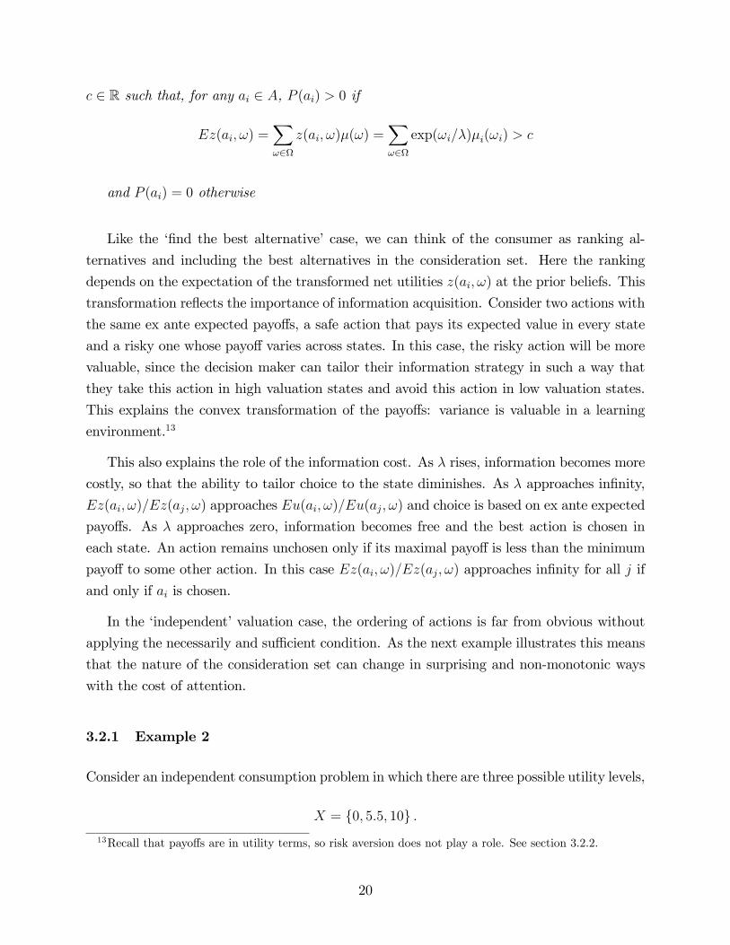
The relationship between attention costs and the associated consideration set is non-

monotonic. For example, for λ = 30 only the safe option is chosen with positive probability,

for λ = 20 both the safe and risky options will be used, for λ = 2 only the risky options

will be used, while for λ = 1 again all options are used. Figure 2 shows the unconditional

probability of the sure thing and each of the risky alternatives being chosen at each value

of λ. It shows 4 different regions for the parameter λ, each of which is related to a different

consideration set. For very low values of λ, when information is very cheap, all alternatives

are used. As λ increases, the probability that the safe option is chosen drops to zero. For

still higher values of λ, the sure thing is once again used, along with the risky options. For

21

the highest values of λ (when information is very expensive) only the sure thing is used.

Figure 2: Unconditional Choice Probabilities in Example 2.14

How is this change occurring, given the condition of Theorem 2? It turns out that

increasing the value of λ has two distinct effects on behavior. First, it can change the

ranking of the the risky and safe options in terms of their normalized utilities given prior

beliefs. At low levels of λ, the risky option dominates the sure thing (the light grey region

in Figure 2). However, as attention costs rise, eventually the normalized utility of the sure

thing moves above that of the risky option (the dark grey region). Thus, for low attention

costs, if only one option is to be used it must be the risky option, while for high costs, only

the sure thing can be used on its own.

A second effect of rising attention costs is to change whether all alternatives are above

the threshold, or just some subset of them: At very low cost levels, all options are above

the threshold. As costs increase, the sure thing drops below the threshold and only the

risky options are used. Further cost rises lead to the sure thing moving back above the cost

threshold.

Some intuition for this effect can be gained from Figure 3. This shows the probability that

the sure thing is chosen conditional on all the risky options being bad, and the probability

that all the risky options are bad conditional on the sure thing being chosen. It illustrates that

14Note that the scale uses increments of 0.1 for λ < 1, and 1 for λ > 1

22

the sure thing plays very different roles in the consideration set at low and high information

cost levels. At low cost levels, when the consumer is very well informed, the sure thing is only

chosen when it is known with high probability that all the risky options are of low quality:

in other words it is only chosen when it is actually the best option. As information costs rise,

at some point it becomes too costly for the consumer to identify such states of the world,

so the sure thing is no longer used. When the sure thing again enters the consideration set

at higher cost levels, it is used in a very uninformed manner. The probability that all the

risky options are bad if the sure thing is chosen is only about 4%, or slightly above the prior

belief that this is the case. In this part of the attention cost region, the sure thing is used

by the consumer as a way of mixing in an uninformed choice with their informed choice in

order to lower costs. As λ rises, use of this uninformed option rises until eventually use of

the risky options ceases.

Figure 3: Conditional Probabilities in Example 2.15

3.2.2 Information Cost and Risk Aversion

Our conditions can also be used to explore the relationship between risk aversion and infor-

mation costs in consideration set formation. Intuitively, such a relationship exists because a

more risk-averse individual requires a higher degree of certainty before they are prepared to

15Note that the scale uses increments of 0.1 for λ < 1, and 1 for λ > 1

23

choose a risky option, and that higher degree of certainty requires more information. Thus,

an investor may be prepared to invest in risky stocks if the have low risk aversion, or low

information costs, but not if they are risk averse and find information costly.

In order to explore this trade off, we can modify the set up of Example 2, so that the

payoffs of each alternative are denominated in monetary units. The risky options pay off $10

and $0 if they are good or bad, while the sure thing pays of $5 for sure. Monetary payoffs

are converted to utility using the function,

u(x) =x1−ρ

1− ρ.

As is standard, the parameter ρ determines the degree of risk aversion, with ρ = 0 equivalent

to risk neutrality.

We can now use Lemma 1 to map out the optimal consideration sets as a function of

λ and ρ. The results are shown in Figure 4, which demonstrates the complex relationship

between the two parameters. Broadly speaking, the intuition described above holds: use

of the risky options increases both with lower information costs and lower risk aversion. At

very low information costs, all options appear in the consideration set. However, at higher

information costs, there are still values for ρ for which all options are chosen with positive

probability. This occurs at intermediate levels of risk aversion, between the ‘risky asset

only’and ‘safe asset only’areas of the parameter space. This region corresponds to the

‘uninformed’use of the safe option described above.

24

Figure 4: Consideration Sets as a Function of ρ and λ

3.3 Consumer Problem 3: Correlated Valuation

The general case in which the value of the different alternatives may be correlated is more

complex. We begin with a geometric interpretation of the model which borrows from Caplin

et al. [2017]. We then present a simple ‘market entry’ test based on Proposition 1. We

conclude this section with an example.

3.3.1 A Geometric Interpretation

Bayes’rule implies a tight relationship between state dependent stochastic choice and poste-

rior beliefs, γa(ω) = P (a|ω)µ(ω)/P (a). We can use this relationship to rewrite problem (1)

replacing P (a|ω) with γa(ω) and P (a). The resulting maximization problem is of the form:

maxP (a)a∈A,γaa∈B(P )

∑a∈B(P )

P (a)∑ω∈Ω

γa(ω)u(a, ω)

−λ[∑a∈A

P (a)∑ω∈Ω

γa(ω) ln γa(ω)−∑ω∈Ω

µ(ω) lnµ(ω)

]

25

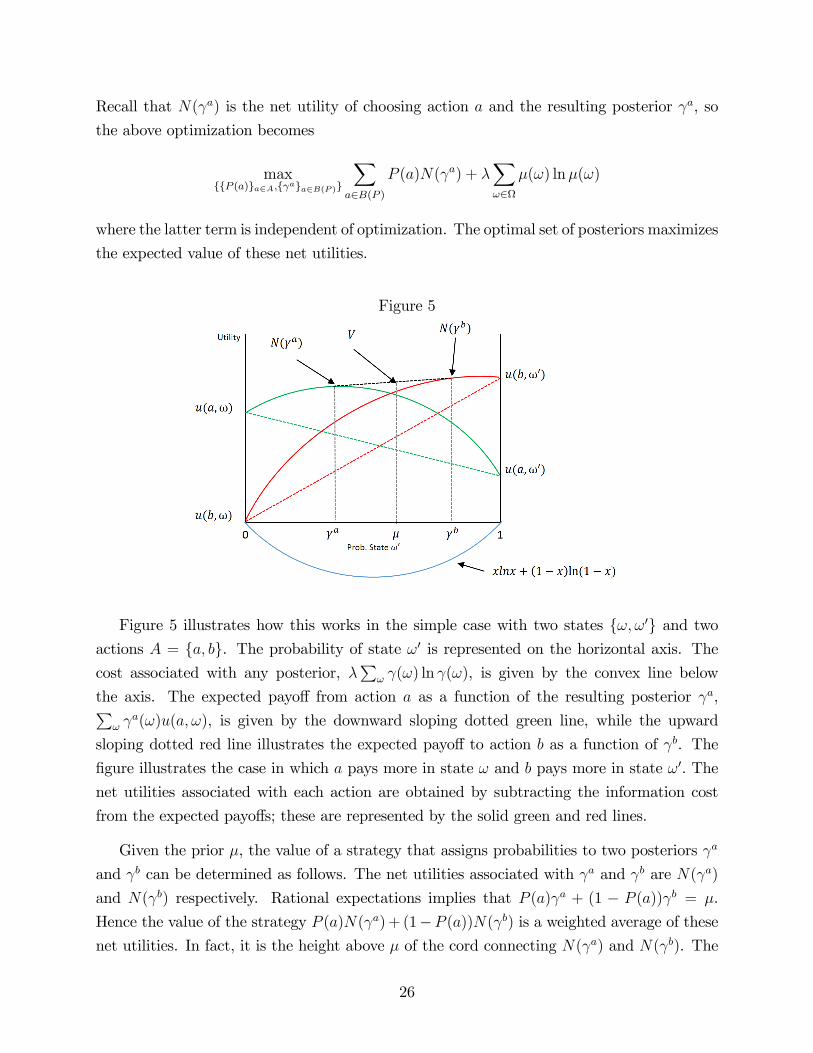
Recall that N(γa) is the net utility of choosing action a and the resulting posterior γa, so

the above optimization becomes

maxP (a)a∈A,γaa∈B(P )

∑a∈B(P )

P (a)N(γa) + λ∑ω∈Ω

µ(ω) lnµ(ω)

where the latter term is independent of optimization. The optimal set of posteriors maximizes

the expected value of these net utilities.

Figure 5

Figure 5 illustrates how this works in the simple case with two states ω, ω′ and twoactions A = a, b. The probability of state ω′ is represented on the horizontal axis. Thecost associated with any posterior, λ

∑ω γ(ω) ln γ(ω), is given by the convex line below

the axis. The expected payoff from action a as a function of the resulting posterior γa,∑ω γ

a(ω)u(a, ω), is given by the downward sloping dotted green line, while the upward

sloping dotted red line illustrates the expected payoff to action b as a function of γb. The

figure illustrates the case in which a pays more in state ω and b pays more in state ω′. The

net utilities associated with each action are obtained by subtracting the information cost

from the expected payoffs; these are represented by the solid green and red lines.

Given the prior µ, the value of a strategy that assigns probabilities to two posteriors γa

and γb can be determined as follows. The net utilities associated with γa and γb are N(γa)

and N(γb) respectively. Rational expectations implies that P (a)γa + (1 − P (a))γb = µ.

Hence the value of the strategy P (a)N(γa) + (1−P (a))N(γb) is a weighted average of these

net utilities. In fact, it is the height above µ of the cord connecting N(γa) and N(γb). The

26

optimal strategy can be found by identifying the posteriors that support the highest possible

chord as it passes over the prior. The posteriors in the figure have this property, and so

would form part of an optimal strategy for this decision problem. Caplin et al. [2017] show

that this insight generalizes to problems with many actions and many states: one graphs

the net utilities and finds the point on the convex hull directly above the prior; the optimal

posteriors are the points of tangency of the supporting hyperplane at this point and the net

utility functions.

Our interest in this paper centers on the implications of this characterization for the

optimal consideration set. In order for an action to be considered, its net utility must touch

the supporting hyperplane. Except in cases of indifference, this means that the net utility

function associated with this action would pierce the hyperplane associated with a problem

that did not include this act. This is clearly more likely if the net utility associated with

this action is higher (i.e. the payoffs are higher) or the plane is lower (i.e. the payoffs to the

other actions are lower). But it also matters in which states the action pays off relative to

the slope of the hyperplane: if the action pays off in states in which the hyperplane is low,

then it will more likely prove valuable.

To see this, Figure 6 illustrates the net utility function for a problem with one act. Since

there is only one action the convex hull of net utility is net utility itself, and the point of

tangency of the supporting plane lies directly above the prior so that the prior is the optimal

posterior. This makes sense since there is no incentive to gather information. The black line

illustrates the supporting plane. A second action will prove valuable if its net utility pierces

this plane, so that the supporting plane to the new problem at µ is higher. When is this

the case? As stated above, clearly an action that pays off more will have a greater chance.

But the new action need not pay off more in all states. Actions tend to be more valuable

if they pay off in states in which the hyperplane is low. There are two reasons that this

may be the case. First, the action in the figure pays off more in state ω, which implies that

net utility tends to slope downward and so the plane tends to be lower in state ω′. Actions

that pay off in state ω′ are therefore more likely to be valuable. This is a hedging motive.

Second, actions that pay off in more likely states are more valuable. In the figure, µ places

more weight on ω′. This shifts the supporting plane to a point on the net utility curve with

greater downward slope so that the plane is lower in ω′. Again actions that pay off in state

ω′ are more likely to be valuable.

27

Figure 6

3.3.2 A Simple ‘Market Entry’Test

Calculating whether a net utility function lies above or below a supporting hyperplane can be

quite involved. Fortunately, the necessary and suffi cient conditions provide a simple test for

whether an action should be added to a consideration set. All unchosen actions a ∈ A\B(P )

must satisfy the inequality ∑ω∈Ω

z(a, ω)µ(ω)∑b∈A P (b)z(b, ω)

≤ 1

We can therefore solve the model without action a and check to see whether this inequality

is satisfied for a. This approach might prove particularly useful in models of market entry

in which the P (b) represent the equilibrium pre-entry.

What types of goods pass the entry test? The following decomposition helps clarify:

∑ω∈Ω

z(a, ω)µ(ω)∑b∈A P (b)z(b, ω)

= Ez(a, ω)+E

(1∑

b∈A P (b)z(b, ω)

)+cov

(z(a, ω),

1∑b∈A P (b)z(b, ω)

).

The first term is familiar from the case of uncorrelated actions: a higher expected level

of z(a, ω) makes an action more desirable. The second term relates to the unconditional

expected value of already chosen actions. This term is the same for all actions and therefore

does not itself distinguish between chosen and unchosen actions. The third term is new and

represents the hedging motive discussed above. A high covariance term means the action

tends to pay off more in states in which other actions pay off less.

28

3.3.3 Example 3

Consider a choice set consisting of three alternatives, a, b and c. The value of each of these

alternatives is determined by an underlying state drawn from Ω = ω1, ω2, each of which isequally likely. The payoff of each action in each state (in utility terms) is described in Table

1.Table 1

Alternative ω1 ω2 E(z(x))

a 5 5 1.65

b 6 0 1.41

c 0 15 2.74

Using Proposition 1, it is easy to show that, for λ = 10, only alteratives b and c will be

in the consideration set - i.e. will be chosen with positive probability. This is despite the

fact that a has a higher expected normalized utility than b at prior beliefs, as can be seen

from the last column of Table 1. The reason for this is that option b provides a better hedge

than a for option c. The presence of option c induces the consumer to find out with high

precision whether the state of the world is ω1 or ω2. Having done so, they sometimes learn

that ω1 is very likely to be the true state, in which case they prefer b to a.16

Example 3 illustrates that the cutoff strategy from Consumer Problem 2 breaks down

because the optimal strategy now potentially depends on all the available actions. Even risk

neutral consumers may utilize the ‘hedging’value of a given act, if it is of high quality in

states where others are low quality. Such actions increase the value to learning, because it

means appropriate action can be taken regardless of what is learned.

In the decision making environment of Example 3, a new alternative will not enter the

consideration set unless it satisfies

1 ≤ 1

2

z(d, ω1)

P (b)z(b, ω1) + P (c)z(c, ω1)+

1

2

z(d, ω2)

P (b)z(b, ω2) + P (c)z(c, ω2)

=1

2

[z(d, ω1)

1.41+z(d, ω2)

2.74

]This condition can then be used to find the ‘minimum cost’way of ensuring that a product

will be enter into the consideration set. In other words, the assignment of u(d, ω1), u(d, ω2) ≥0 which guarantees that d be in the consideration set, while minimizing the expected utility

of d at prior beliefs. In the above example, it is clear that the solution to this problem is to

16A similar example appears in Matejka and McKay [2015].

29

set u(d, ω2) = 0 and set u(d, ω1) in order to make 12z(d,ω1)

1.41= 1. This allocation puts maximal

utility on the state which has the lowest expected value of normalized utility given current

choice patterns.

4 The ILR Conditions, Priors, and Consideration Sets

One feature that makes the Shannon model diffi cult to solve is the necessity of finding sets

of posteriors that average to the prior. This complicates finding the optimal consideration

set associated with any given prior. It turns out that the converse problem of finding priors

associated with any given consideration set is somewhat simpler to characterize. In this

section we show how the ILR conditions partition ∆(Ω) into sets of priors, each of which is

associated with a given consideration set. For simplicity we consider only cases in which the

uniqueness condition of Remark 1 holds, meaning that there is a unique optimal consideration

set consistent with each decision problem.

Define

f(x; a, b) =∑ω∈Ω

[z(b, ω)

z(a, ω)

]x(ω)

where x ∈ R|Ω| and a, b ∈ A, and consider the equation

f(x; a, b) = 1. (11)

This equation defines a plane of dimension |Ω| − 1 in R|Ω| which divides R|Ω| into two sets:one in which f(x; a, b) > 1, and another in which f(x; a, b) < 1. If both a and b are chosen,

the ILR conditions, γa(ω)z(a,ω)

= γb(ω)z(b,ω)

, imply that,

f(γa; a, b) =∑ω∈Ω

[z(b, ω)

z(a, ω)

]γa(ω) =

∑ω∈Ω

γb(ω) = 1.

Hence f(γa; a, b) = 1 implicitly defines the set of possible posteriors γa for action a such

that both action a and action b are chosen with positive probability. Moreover, according to

the likelihood ratio inequalities for unchosen options, the set of γa such that f(γa; a, b) ≤ 1,

represent the set of possible posteriors for action a such that a is chosen and b is not chosen.

30

Figure 7

Figure 7 illustrates (11) for Consumer Problem 1 of section 3.1 with three states and

three actions. It shows a two dimensional representation of the probability simplex from

R3. The vertices are the points (1,0,0), (0,1,0) and (0,0,1). Recall that utility is high, uG,

if the index on the state matches the index on the act and low, uB, otherwise. With these

payoffs, the plane f(x; a1, a3) = 1 intersects the simplex along the solid line in the figure.17

This divides the simplex into two regions. In the shaded region, f(x; a1, a3) < 1. In the

other region f(x; a1, a3) > 1. In this example, the solid line runs through the point x = ω2

because a1 and a3 are equivalent in state ω2 and soz(a3,ω2)z(a1,ω2)

= uBuB

= 1. The points along

the solid line are the potential γa1 for which the ILR conditions may hold for both actions

a1 and a3. The shaded region represents the potential γa1 that are consistent with action

a1 being chosen and action a3 not being chosen. The dashed line represents the points at

which f(x; a1, a2) = 1. This represents the set of the potential values for γa1 for which the

ILR conditions may hold for actions a1 and a2. The point A lies at the intersection of the

two lines. If all three actions are chosen, then we must have γa1 = A.

We now show how the inequalities partition ∆(Ω) into priors which support different

consideration sets. Given a non-empty subset B ⊆ A, define SB ⊆ ∆(Ω) as the set of

priors for which B is the consideration set. Note that this set may be empty if B is not

the consideration set for any prior. We show now how our understanding of the sets of

17In general, the plane will contain the simplex if z(a, ω) = z(b, ω) for all ω, and the plane will fail tointersect the simplex if z(a, ω) > z(b, ω) or z(a, ω) > z(b, ω) for all ω.

31

posteriors that are associated with a given consideration set allows us to characterizes thecorresponding priors as the set of all convex combinations.

The convexification operation is somewhat subtle to specify. The first step is to choose

a ∈ B and to define ΓaB as the set of posteriors for action a which are consistent with the

consideration set B,

ΓaB = x ∈ ∆(Ω) |f(x; a, b) ≤ 1 for all b ∈ A\a with equality for b ∈ B\a . (12)

The second step is to select γa ∈ ΓaB, and then use the ILR conditions to generate γb(γa) for

all b ∈ B as follows:

γb(ω) =z(b, ω)

z(a, ω)γa(ω)

For b = a, this is simply the identity mapping.

The key result is that for B to be the consideration set, µ must lie in the interior of the

convex hull of the γb(γa) for some γa ∈ ΓaB. The proof is in the appendix. Note that the

symmetry of the ILR conditions imply that the particular choice of a ∈ B is inconsequentialto this construction.

Theorem 3 Given µ ∈ ∆(Ω), B is the consideration set for the decision problem (µ,A) if

and only if, given, a ∈ B,

µ ∈ SB = ∪γa∈ΓaBintconvγb(γa)|b ∈ B

Figure 8 illustrates this construction for the consumer problem in section 3.1 with three

states and three actions. First consider SA. This is the set of priors for which all actions

are chosen. Since all actions are chosen f(x; a, b) = 1 for all a and b. The solid blue lines

ω2H and ω3D show the intersection of the planes f(x; a1, a3) = 1 and f(x; a1, a2) = 1 with

the simplex. Their intersection pins down γa1 at point A. This point is Γa1A . Similarly the

dashed red lines pin down γa2 at B and and the dot-dashed green lines pin down γa3 at C.

SA corresponds to the interior of the convex hull of these three points, which is the interior of

the triangle ABC in the figure. Note that every point in ABC is equal to the average of the

points A, B and C with strictly positive weights. These weights are the action probabilities

P (a) from the optimal strategy. On the boundary of ABC some action probability falls to

zero and the consideration set shrinks.

Now consider Sa1,a2. Γa1

a1,a2 is the set of points for which f(x; a1, a2) = 1 and f(x; a1, a3) ≤1. This corresponds to the line segment AD in the figure. The ILR conditions map AD

32

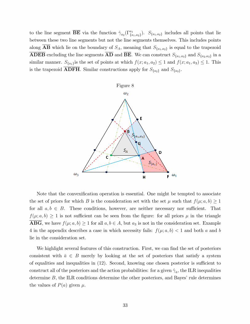
to the line segment BE via the function γa2(Γa1

a1,a2). Sa1,a2 includes all points that lie

between these two line segments but not the line segments themselves. This includes points

along AB which lie on the boundary of SA, meaning that Sa1,a2 is equal to the trapezoid

ADEB excluding the line segments AD and BE. We can construct Sa1,a3 and Sa2,a3 in a

similar manner. Sa1is the set of points at which f(x; a1, a2) ≤ 1 and f(x; a1, a3) ≤ 1. This

is the trapezoid ADFH. Similar constructions apply for Sa2 and Sa3.

Figure 8

Note that the convexification operation is essential. One might be tempted to associate

the set of priors for which B is the consideration set with the set µ such that f(µ; a, b) ≥ 1

for all a, b ∈ B. These conditions, however, are neither necessary nor suffi cient. That

f(µ; a, b) ≥ 1 is not suffi cient can be seen from the figure: for all priors µ in the triangle

ABG, we have f(µ; a, b) ≥ 1 for all a, b ∈ A, but a3 is not in the consideration set. Example

4 in the appendix describes a case in which necessity fails: f(µ; a, b) < 1 and both a and b

lie in the consideration set.

We highlight several features of this construction. First, we can find the set of posteriors

consistent with a ∈ B merely by looking at the set of posteriors that satisfy a system

of equalities and inequalities in (12). Second, knowing one chosen posterior is suffi cient to

construct all of the posteriors and the action probabilities: for a given γa, the ILR inequalities

determine B, the ILR conditions determine the other posteriors, and Bayes’rule determines

the values of P (a) given µ.

33

Finally, the construction illustrates that the conditions under which all actions are taken

are very strict. If there are as many actions as states and since the normalized payoffs

are linearly independent, ΓaA can only contain one posterior. This posterior determines the

others through the ILR conditions which then determines the set of priors consistent with

all actions being chosen. Any other priors will leave some action unchosen. Moreover, this

set shrinks toward the uniform distribution as the payoffs to all become more similar.

5 Literature Review

Our paper provides new techniques for solving models of rational inattention which have been

popular in economics since their introduction by Sims [2003].18 Specifically, we augment the

results of Matejka and McKay [2015] to provide conditions which are both necessary and

suffi cient for optimality (see also Stevens [2014]).

Within the literature on rational inattention, our results are related to the recent work

by Jung et al. [2015] (henceforth JKMS). They show that in a wide class of models in

which the state of the economy is continuous (or multi-variate) and the full information

optimal policy would be a continuous function of this state, the optimally inattentive policy

is instead discrete (or of lower dimension). Like our paper, JKMS begin with the observation

that a rationally attentive decision maker may choose only a subset of the available actions.

Whereas our focus is on the characteristics of the chosen actions, JKMS provide conditions

under which the consideration set B is of lower dimension than the action space A or the

uncertainty Ω. Their conditions involve the smoothness of the payoff function —they require

the payoffs to be analytic and integrable —conditions that have no bite when the state space

is finite.

There are several recent papers that have tackled the concept of consideration sets from

a theoretical perspective. Masatlioglu et al. [2012] (henceforth MNO) take a ‘revealed pref-

erence’ approach, using the identifying assumption that if an alternative x is not in the

consideration set for some choice set S, removing x will not change the consideration set.

They use this condition to provide necessary and suffi cient conditions for a data set to be

consistent with choice from consideration sets.19 Unlike our approach, consideration sets in

MNO do not come about as the result of optimizing behavior, although our model does sat-

18See for example the application of the model to investment decisions (e.g van Nieuwerburgh and Veld-kamp [2009]), global games (Yang [2015]), pricing decisions (Mackowiak and Wiederholt [2009], Matejka[2015], Martin [2017]), and delegation (Lindbeck and Weibull [2017]).19See Lleras et al. [2017] and Dean et al. [2017] for similar approaches.

34

isfy their identifying restriction. This means on the one hand that their model is potentially

more flexible, while on the other it provides fewer comparative static predictions. MNO also

assume the absence of mistakes within the consideration set. A combination of deterministic

consideration sets and preference maximization mean that MNO’s model predict that choice

will be deterministic. More recently, Demuynck and Seel [2017] have also taken a revealed

preference approach to consideration set formation, in which they assume that some com-

modities in a bundle may not be observed, while the literature on demand estimation has

taken various different approaches to identifying consideration sets (see for example Goeree

[2008] and Abaluck and Adams [2017]). These papers also treat the consideration set as

exogenous, rather than deriving from some optimizing process.

Another recent approach is that of Manzini and Mariotti [2014], who assume that consid-

eration sets are formed stochastically, with any given alternative having a fixed probability of

being considered. Again, consideration is not the result of optimization, and choice within

the consideration set is always optimal, but the random nature of consideration leads to

random choice. Unlike our model, all alternatives are always chosen, meaning that, by our

definition, all alternatives are in the consideration set. On a technical level, our model would

violate the I-Asymmetry and I-independence axioms of Manzini and Mariotti [2014]. This

is because the Manzini-Mariotti model is based on the existence of an underlying, state

independent ranking over alternatives. This ranking can be uncovered from particular ob-

servations in the data, and axioms then place consistency requirements on the resulting

revealed preference relations. Because our model has no such ranking it is easy to construct

examples by which alternative x is strictly revealed preferred to alternative y (according to

the Manzini-Mariotti model) and visa versa. Similar reasoning means that our model is dis-

tinct from the Menu-Dependent Stochastic Feasibility model of Brady and Rehbeck [2016],

a variant of the Manzini-Mariotti model.20

A further model of consideration set formation is the search and satisficing approach,

originally suggested by Simon [1955]. In such a model, alternatives are considered one by

one until one is found which is ‘good enough’. As discussed in Caplin et al. [2011], satisficing

can be seen as the result of an optimizing procedure in the face of information costs. While

this paper considers only the case in which alternatives are ex ante identical, Gabaix et al.

[2006] discuss the extension to a situation in which the decision maker may have different

priors about the quality of different alternatives. However, the same paper shows that

extending this model to the case in which search only reveals partial information about the

quality of the alternative is generally intractable.

20Our model could, for example generate violations of the Asymmetric Sequential Independence axiom.

35

Their is a much longer history of research into consideration sets in marketing. Classic

examples include Roberts and Lattin [1991] and Hauser and Wernerfelt [1990]. Typically,

these papers run into the same tractability problems discussed in Gabaix et al. [2006]. These

are solved by making strong distributional assumptions on the nature of information, and

using this to derive various moments of the choice distribution. As far as we are aware,

none of these papers have considered the approach of using rational inattention to model

consideration set formation.

6 Conclusion

We introduce new necessary and suffi cient conditions for the solution of the Shannon model.

These conditions allow for the identification of the set of actions that will be chosen with

positive probability at the optimum. We follow up on this by using the model to analyze

optimal consideration set formation. This allows us to identify the optimal consideration

set and the optimal pattern of mistakes within the consideration set in a tractable and

reasonable manner. The results may be of interest for those in economics and marketing

analyzing properties of demand systems.

36

References

Jason Abaluck and Abi Adams. What do consumers consider before they choose? identifi-

cation from asymmetric demand responses. 2017.

Marina Agranov and Pietro Ortoleva. Stochastic choice and preferences for randomization.

Journal of Political Economy, 125(1):40—68, 2017.

Marina Agranov and Pietro Ortoleva. Stochastic choice and preferences for randomization.

Journal of Political Economy, 125(1):40—68, 2017.

Jose Apesteguia, Miguel A Ballester, and Jay Lu. Single-crossing random utility models.

Econometrica, 85(2):661—674, 2017.

Richard L Brady and John Rehbeck. Menu-dependent stochastic feasibility. Econometrica,

84(3):1203—1223, 2016.

Andrew Caplin and Mark Dean. Behavioral implications of rational inattention with shannon

entropy. NBER Working Papers 19318, National Bureau of Economic Research, Inc,

August 2013.

Andrew Caplin, Mark Dean, and Daniel Martin. Search and satisficing. The American

Economic Review, 101(7):2899—2922, 2011.

Andrew Caplin, Mark Dean, and John Leahy. Rationally inattentive behavior: Characteriz-

ing and generalizing shannon entropy. 2017. Unpublished.

Raj Chetty, Adam Looney, and Kory Kroft. Salience and taxation: Theory and evidence.

American Economic Review, 99(4):1145—1177, 2009.

Andrew Ching, Tülin Erdem, and Michael Keane. The price consideration model of brand

choice. Journal of Applied Econometrics, 24(3):393—420, 2009.

Thomas M Cover and Joy A Thomas. Elements of information theory. John Wiley & Sons,

2012.

Geoffroy De Clippel, Kfir Eliaz, and Kareen Rozen. Competing for consumer inattention.

Journal of Political Economy, 122(6):1203—1234, 2014.

Mark Dean, Özgür Kıbrıs, and Yusufcan Masatlioglu. Limited attention and status quo bias.

Journal of Economic Theory, 169:93—127, 2017.

37

Thomas Demuynck and Christian Seel. Revealed preference with limited consideration.

American Economic Journal: Microeconomics, 2017.

Kfir Eliaz and Ran Spiegler. Consideration sets and competitive marketing. The Review of

Economic Studies, 78(1):235—262, 2011.

Xavier Gabaix, David Laibson, Guille Moloche, and Stephen Weinberg. Costly information

acquisition: Experimental analysis of a boundedly rational model. American Economic

Review, 96(4):1043—1068, 2006.

Martin Gaynor, Carol Propper, and Stephan Seiler. Free to choose? reform, choice, and

consideration sets in the english national health service. The American Economic Review,

106(11):3521—3557, 2016.

Sen Geng. Decision time, consideration time, and status quo bias. Economic Inquiry,

54(1):433—449, 2016.

Michelle Sovinsky Goeree. Limited information and advertising in the us personal computer

industry. Econometrica, 76(5):1017—1074, 2008.

John R. Hauser and Birger Wernerfelt. An evaluation cost model of consideration sets.

Journal of Consumer Research, 16(4):pp. 393—408, 1990.

Wayne D. Hoyer. An examination of consumer decision making for a common repeat purchase

product. Journal of Consumer Research, 11(3):pp. 822—829, 1984.

Junehyuk Jung, Jeong-Ho Kim, Filip Matejka, Christopher A Sims, et al. Discrete actions

in information-constrained decision problems. Technical report, working paper, 2015.

Nicola Lacetera, Devin Pope, and Justin Sydnor. Heuristic thinking and limited attention

in the car market. American Economic Review, 102(5):2206—2236, 2012.

Assar Lindbeck and Jörgen Weibull. Delegation to a rationally inattentive agent. Technical

report, 2017.

Juan Sebastian Lleras, Yusufcan Masatlioglu, Daisuke Nakajima, and Erkut Y Ozbay. When

more is less: Limited consideration. Journal of Economic Theory, 170:70—85, 2017.

Bartosz Mackowiak and Mirko Wiederholt. Optimal sticky prices under rational inattention.

American Economic Review, 99(3):769—803, June 2009.

Paola Manzini and Marco Mariotti. Stochastic choice and consideration sets. Econometrica,

82(3):1153—1176, 2014.

38

Paola Manzini and Marco Mariotti. Dual random utility maximisation. 2016.

Daniel Martin. Strategic pricing with rational inattention to quality. Games and Economic

Behavior, 104:131—145, 2017.

Yusufcan Masatlioglu, Daisuke Nakajima, and Erkut Y Ozbay. Revealed attention. American

Economic Review, 102(5):2183—2205, 2012.

Filip Matejka and Alisdair McKay. Rational inattention to discrete choices: A new founda-

tion for the multinomial logit model. American Economic Review, 105(1):272—98, 2015.

Filip Matejka. Rationally inattentive seller: Sales and discrete pricing. The Review of

Economic Studies, 83(3):1156—1188, 2015.

Frederick Mosteller and Philip Nogee. An experimental measurement of utility. The Journal

of Political Economy, pages 371—404, 1951.

Elena Reutskaja, Rosemarie Nagel, Colin F Camerer, and Antonio Rangel. Search dynamics

in consumer choice under time pressure: An eye-tracking study. The American Economic

Review, 101(2):900—926, 2011.

John H. Roberts and James M. Lattin. Development and testing of a model of consideration

set composition. Journal of Marketing Research, 28(4):pp. 429—440, 1991.

Babur De Los Santos, Ali Hortaçsu, and Matthijs Wildenbeest. Testing models of consumer

search using data on web browsing and purchasing behavior. American Economic Review,

102(6):2955—2980, Oct 2012.

Herbert Simon. A behavioral model of rational choice. The Quarterly Journal of Economics,

69(1):99—118, Feb 1955.

Christopher A. Sims. Implications of Rational Inattention. Journal of Monetary Economics,

50(3):665—690, 2003.

Luminita Stevens. Coarse pricing policies. Available at SSRN 2544681, 2014.

Constantino Tsallis. Possible generalization of boltzmann-gibbs statistics. Journal of statis-

tical physics, 52(1-2):479—487, 1988.

Stijn van Nieuwerburgh and Laura Veldkamp. Information immobility and the home bias

puzzle. Journal of Finance, 64(3):1187—1215, 06 2009.

Ming Yang. Coordination with flexible information acquisition. Journal of Economic Theory,

158:721—738, 2015.

39

7 Appendix

Proof of Theorem 1 . A necessary condition for chosen set B ⊂ A to be optimal is that,

for each a ∈ B, ∑ω∈Ω

z(a, ω)∑b∈A P (b)z(b, ω)

µ(ω) = 1

Substituting in the specific payoffs, the key equation has simple form,

∑ω∈Ω

z(a, ω)∑b∈A P (b)z(b, ω)

µ(ω) =x(1 + δ)µi

x(1 + δP (ai))+

∑aj∈B\ai

xµjx(1 + δP (aj))

+∑

ak∈A\B

µk

=δµi

1 + δP (ai)+∑aj∈B

µj(1 + δP (aj))

+∑

ak∈A\B

µk = 1.

In light of the fact that the sum of all priors is 1 we can subtract∑

ak∈A\B µk from both

sides and define the key ratio,

ρi =µi

1 + δP (ai),

for all ai ∈ B, we arrive at,

δρi +∑aj∈B

ρj =∑aj∈B

µj =⇒ ρi =

∑aj∈B µj −

∑aj∈B ρj

δ.

Note that the RHS above is independent of ai. Hence all ρj for aj ∈ B are identical,

whereupon substitution yields,

ρi =

∑aj∈B µj

|B|+ δ.

We can back out the implied probabilities for ai ∈ B as,

1 + δP (ai) =µiρi

=µi (|B|+ δ)∑

ak∈B µk;

so that,

P (ai) =µa (|B|+ δ)

δ∑

ak∈B µk− 1

δ.

We now apply analogous logic to unchosen options ai ∈ A\B for which the corresponding

40

necessary inequality is,

∑ω∈Ω

z(a, ω)∑b∈A P (b)z(b, ω)

µ(ω) =∑aj∈B

µj(1 + δP (aj))

+∑

ak∈A\B

µk + δµi ≤ 1,

Substituting the known value of ρj for aj ∈ B and subtracting∑

aj∈A\B µj from both sides

in light of the fact that the sum of all priors is 1 we arrive at,

δµi ≤∑aj∈B

[µj −

µj(1 + δP (aj))

]=∑aj∈B

[µj − ρj

]=

∑aj∈B

[µj −

∑aj∈B µj

|B|+ δ.

]=δ∑

aj∈B µj

|B|+ δ.

We conclude that the necessary and suffi cient conditions for optimality are satisfied by

the specification of a set of chosen options B ⊂ A if and only if the implied probabilities of

chosen options a ∈ B are all non-negative,

ai ∈ B =⇒ µi >

∑k∈B µk

(|B|+ δ).

while the corresponding inequality is satisfied by unchosen options ,

aj ∈ A\B =⇒ µj ≤∑

k∈B µk(|B|+ δ)

.

Note that if µM > 1M+δ

, then setting B = A verifies all conditions. Otherwise, if µM ≤1

M+δ, then we identify integer K < M such that,

µK >

∑Kk=1 µkK + δ

≥ µK+1.

To see that there is such an integer, note first that µ1 >µ1

1+δ, and that,

µM ≤∑K

k=1 µkM + δ

=1

M + δ.

Hence one can count up from k = 1 to identify the smallest integer K < M such that,

µK >

∑Kk=1 µkK + δ

≥ µK+1.

41

With such K identified, the fact that µK >∑Kk=1 µkK+δ

verifies that the same is true for all

ai ∈ A for which µi ≥ µK , while the fact that µK+1 ≤∑Kk=1 µkK+δ

verifies that the same is

true for all aj ∈ A for which µj ≤ µK . Hence we have satisfied all necessary and suffi cient

conditions to identify action set B = 1, 2, .., K and corresponding probabilities P (ai) > 0

on ai ∈ B to characterize the optimal attention strategy.

Note that for ai ∈ B the posteriors satisfy,

γi(ωj) =z(ai,, ωj)µj∑K

k=1 P (ak)z(ak, ωj).

Hence, for b = a,

γi(ωi) =x(1 + δ)µi∑K

k=1 P (ak)z(ak, ωj)=

x(1 + δ)µix(1 + δP (ai))

= (1 + δ)ρi =(1 + δ)

∑k µk

K + δ.

Moreover for b 6= a and b ≤ K,

γi(ωj) =xµj∑K

k=1 P (ak)z(ak, ωj)=

xµjx(1 + δP (ai))

= ρi =

∑k µk

K + δ.

Finally, for b > K,

γi(ωj) =xµj∑K

k=1 P (ak)z(ak, ωj)=xµix

= µj.

This completes the proof.

Proof of Theorem 2 The proof is by contradiction. The expected utility of an actionai at prior beliefs is

E(u(ai, ω)) =∑ω∈Ω

u(ai, ω)µ(ω) =∑ωj∈X

ωjµi(ωj).

Independence implies that this expression is independent of any other action. The same is

true of the expected value of the normalized utilities z(a, ω) ≡ exp(u(a, ω)/λ).

We use Ezai to refer to this expectation,

Ezai =∑ωj∈X

exp(ωj/λ)µi(ωj).

Suppose that there exist two actions ak and al such that Ezak < Ezal and yet ak is chosen

42

with positive probability and al is not. Define

Σ(ω) =

(∑ai∈B

P (ai)z(ai, ω)

)−1

.

The necessary and suffi cient conditions imply

EzakΣ =∑ω∈Ω

[z(ak, ω)

Σ(ω)µ(ω)

]= 1 ≥

∑ω∈Ω

[z(al, ω)

Σ(ω)µ(ω)

]= EzalΣ.

The fact that al is not chosen means that al /∈ B, which implies that Σω is independent of

z(al, ω), as Σ(ω) is a function of z(ai, ω) for every ai ∈ B, all of which are independent ofz(al, ω). It follows that

EzalΣ = EzalEΣ.

Furthermore, by assumption

EzalEΣ > EzakEΣ,

so that,

EzakΣ > EzakEΣ,

which can only hold if,

cov(zak ,Σ) > 0.

By definition:

cov(zak ,Σ) ≡ Ezak − Ezak∑

ai∈B P (ai)z(ai, ω)

= Ezak − Ezak

P (ak)z(ak, ω) +∑

ai∈B/ak P (ai)z(ai, ω)

= E

E zak − EzakP (ak)z(ak, ω) +

∑ai∈B/ak P (ai)z(ai, ω)

∣∣∣∣∣ ∑ai∈B/ak

P (ai)z(ai, ω)

= E

cov(zak ,

1

P (ak)z(ak, ω) +∑

ai∈B/ak P (ai)z(ai, ω)

)∣∣∣∣∣ ∑ai∈B/ak

P (ai)z(ai, ω)

;

where the second to last line follows from the law of iterated expectations and the last line

follows from the independence of ak and the other elements of B which implies that Ezak

is independent of∑

ai∈B/ak P (ai)z(ai, ω). For given∑

ai∈B/ak P (ai)z(ai, ω) it is clear that

cov(zak , 1

P (ak)z(ak,ω)+∑ai∈B/ak

P (ai)z(ai,ω)

)is negative. As the expectation of a collection of

43

negative numbers is negative,

cov(zak ,Σ) < 0.

This contradiction establishes the proof.

Proof of Lemma 1 First we show that a strategy of choosing a ∈ B with probability1Nsatisfies the necessary and suffi cient conditions of Proposition 1 for all a ∈ B. Given the

proposed strategy and the independence of the decisions

∑ω∈Ω

z(a, ω)µ(ω)∑b∈B P (b)z(b, ω)

=∑ω∈Ω

z(a, ω)ΠMi=1µi(ωi)∑

b∈B1Nz(b, ω)

for all a ∈ B. The denominator depends only on the first N elements of the state vector, so

we can sum across the other states giving,

∑x∈XN

exp (xa/λ) ΠNi=1µB(xi)

1N

[∑Ni=1 exp (xi/λ)

] . (13)

We now subdivide XN into equivalence classes as follows: given x1, x2 ∈ XN then x1 and x2

are members of the same equivalence class X if x2 is a permutation of x1. We rewrite (13)

∑X

∑x∈X

exp (xa/λ) ΠNi=1µB(xi)

1N

[∑Ni=1 exp (xi/λ)

] .Note that conditional on x ∈ X, the denominator,

∑Ni=1 exp (xi/λ), and the probability,

ΠNi=1µB(xi), are constant. Therefore

∑X

∑x∈X

exp (xa/λ) ΠNi=1µB(xi)

1N

[∑Ni=1 exp (xi/λ)

] =∑X

ΠNi=1µB(xi)

∑x∈X exp (xa/λ)

1N

[∑Ni=1 exp (xi/λ)

]

∑X

∑x∈X

N exp (xa/λ)µ(X)

|X|[∑N

i=1 exp (xi/λ)]

=∑X

µ(X)N∑

x∈X exp (xa/λ)

|X|∑N

i=1 exp (xi/λ).

Let µ(X) denote the probability x ∈ X. We have µ(X) = |X|ΠNi=1µB(xi). Note also that∑

x∈X exp (xa/λ) and∑N

i=1 exp (xi/λ) share common terms in common proportions. The

44

only difference is the frequency in which these terms appear.∑

x∈X exp (xa/λ) has |X| termsand

∑Ni=1 exp (xi/λ) has N terms.

∑x∈X exp (xa/λ) /

∑Ni=1 exp (xi/λ) is therefore equal to

|X|/N . Substituting these results, we have

∑X

ΠNi=1µB(xi)

∑x∈X exp (xa/λ)

1N

[∑Ni=1 exp (xi/λ)

] =∑X

µ(X)

|X| |X|1NN

=∑X

µ(X) = 1.

Hence the conditions of Proposition 1 hold for a ∈ B.

To complete the proof we need to show that for all a ∈ A\B,

∑ω∈Ω

z(a, ω)µ(ω)∑b∈A P (b)z(b, ω)

≤ 1.

Given independence and the proposed strategy this becomes,

∑x∈X

exp(x/λ)µa(x)∑x∈XN

ΠNi=1µB(xi)

1N

∑Ni=1 exp (xi/λ)

≤ 1.

This relationship holds given the conditions of the lemma, completing the proof.

Proof of Theorem 3

We first prove that if B is the optimal consideration set for some prior µ ∈ ∆(Ω), then

µ ∈ SB. Suppose that µ ∈ ∆(Ω) and suppose that B is the optimal consideration set. This

means that there exists P (a)a∈A with B(P ) = B and γaa∈B which satisfy the conditions

of Proposition 2. Fix a ∈ B and consider γa. The ILR conditions imply that for any b ∈ B\a

f(γa; a, b) ≡∑ω∈Ω

[z(b, ω)

z(a, ω)

]γa(ω) =

b∑ω∈Ω

γb(ω) = 1

and the likelihood ratio inequalities imply that for any c 6∈ Ω

f(γa; a, c) ≡∑ω∈Ω

[z(c, ω)

z(a, ω)

]γa(ω) ≤ 1

Hence γa ∈ ΓaB. The ILR conditions imply that

γb(ω) =z(b, ω)

z(a, ω)γa(ω)

45

hence γb = γb(γa). Bayes’rule implies that

µ(ω) =∑b∈B

P (b)γb(ω)

Since all actions b ∈ B are chosen, it follows that

µ ∈ intconvγb(γa)|b ∈ B

and hence µ ∈ SB.

We now show that if µ ∈ SB then B is the optimal consideration set. Suppose that

µ ∈ SB. There exists a ∈ B, γa ∈ ΓaB, γb = γb(γa) and P (b) > 0 such that

µ(ω) =∑b∈B

P (b)γb(ω).

We need to show that the γb lie in the simplex and satisfy the ILR conditions for chosen

acts and the likelihood ratio inequalities for unchosen acts. To see that γb ∈ ∆(Ω), note first

that γa ∈ ΓaB implies γa ∈ ∆(Ω). Now z(b, ω) = exp(u(b,ω))

λ> 0 for all b ∈ A and ω ∈ Ω, so

γb(ω) =z(b, ω)

z(a, ω)γa(ω) ≥ 0.

Finally, ∑ω∈Ω

γb(ω) =∑ω∈Ω

z(b, ω)

z(a, ω)γa(ω) = f(γa; a, b) = 1

where the final equality follows from the fact that γa ∈ ΓaB. Hence γb ∈ ∆(Ω). The ILR

conditions hold by construction. Consider b ∈ B and c ∈ A\B

∑ω∈Ω

[γb(ω)

z(b, ω)

]z(c, ω) =

∑ω∈Ω

[z(c, ω)

z(a, ω)

]γa(ω) ≤ 1

where the first equality follows from the construction of γb and the second from the definition

of ΓaB. Hence the likelihood ratio inequalities hold as well. We conclude the B is the

consideration set. This completes the proof of the Theorem.

46

7.1 Example 4

Consider a symmetric tracking problem with 21 states with labels −10, 9, 8 . . . 0, . . . 10.Suppose that the loss function is quadratic in the distance between the guess a and the state

ω,

u(a, ω) = −‖(a, ω)‖2 ,

and that λ = 10. Finally suppose that the prior µ has a truncated Cauchy distribution, the

density of which is,1

c

1

4(ω − 11)2 + 1,

where c is a constant of integration. This density is centered at zero.

In this case, the optimal policy is approximately

P (0) = 0.9859302

P (−9) = P (9) = 0.0065017

P (−10) = P (10) = 0.0005332

Given the weight that the Cauchy distribution places on zero relative to its neighbors (in

this case µ(0) = .6 and µ(1) = .12), it is optimal to pick zero with a high probability, and not

pick anything close to zero. But given the fat tails of the Cauchy distribution, it is optimal

to pick something far from zero, and since the distribution is relatively flat far from zero (in

this case µ(9) = .0018 and µ(10) = .0015) it is optimal to pick neighboring points.

In this example a9 and a10 are both chosen with positive probability and the likelihood

ratio inequalities are satisfied,

f(γa9 , a9, a10) = 1,

but,

f(µ, a9, a10) = .6766 < 1.

So, it is not true that a and b both being considered implies,

f(µ, a, b) ≥ 1.

The explanation is that γa9 is very different than µ:

γa9(0) = .0002 and µ(0) = .6005

γa9(8) = .2247 and µ(8) = .0023

47

An implication is that introducing an additional action can bring an unchosen action to life.

If the only available choices were a9 and a10, a9 would be chosen with probability one and

a10 would not be chosen. The addition of a0 to the choice set, however, moves the posterior

associated with a9 until a10 is chosen as well.

48