Rational Inattention when Decisions Take Time

Rational Inattentionwhen Decisions Take Time∗

Benjamin Hébert †

Stanford University

Michael Woodford ‡

Columbia University

July 30, 2021

Abstract

Decisions take time, and the time taken to reach a decision is likely to be informa-

tive about the cost of more precise judgments. We formalize this insight in the context

of a dynamic model of optimal evidence accumulation. We provide conditions under

which the resulting belief dynamics resemble either diffusion processes or processes

with large jumps. We then demonstrate that the state-contingent choice probabilities

predicted by our model are identical to those predicted by a static rational inatten-

tion model, providing a micro-foundation for such models. In the diffusion case, our

model provides a normative foundation for a variant of the drift-diffusion model from

mathematical psychology.

∗The authors would like to thank Mark Dean, Sebastian Di Tella, Mira Frick, Xavier Gabaix, MatthewGentzkow, Mike Harrison, Emir Kamenica, Divya Kirti, Jacob Leshno, Stephen Morris, Pietro Ortoleva,José Scheinkman, Ilya Segal, Ran Shorrer, Joel Sobel, Miguel Villas-Boas, Ming Yang, and participants atthe Cowles Theory conference, 16th SAET Conference, Barcelona GSE Summer Conference on StochasticChoice, Stanford GSB research lunch, 2018 ASSA meetings, UC Berkeley Theory Seminar, and UC SanDiego Theory for helpful discussions on this topic, Tianhao Liu for excellent research assistance, and the NSFfor research support. We would particularly like to thank Philipp Strack and Doron Ravid for discussing anearlier version of the paper, and Simon Kelly for sharing data from Kelly et al. [2021]. Portions of this papercirculated previously as the working papers “Rational Inattention with Sequential Information Sampling,”“Rational Inattention in Continuous Time,” and “Information Costs and Sequential Information Sampling,”and appeared in Benjamin Hébert’s Ph.D. dissertation at Harvard University. All remaining errors are ourown.†Hébert: Stanford University. Email: [email protected].‡Woodford: Columbia University. Email: [email protected].

1 Introduction

It is common in economic modeling to assume that, when presented with a choice set, adecision maker (DM) will choose the option that is ranked highest according to a coherentpreference ordering. However, observed choices in experimental settings often appear tobe random, and while this could reflect random variation in preferences, it is often moresensible to view choice as imprecise. Models of rational inattention (such as Matêjka et al.[2015]) formalize this idea by assuming that the DM chooses her action based on a signalthat provides only an imperfect indication of the true state. The information structure thatgenerates this signal is optimal, in the sense of allowing the best possible joint distributionof states and actions, net of a cost of information. In the terminology of Caplin and Dean[2015], models of rational inattention make predictions about patterns of state-dependentstochastic choice. These predictions will depend in part on the nature of the informationcost, and several recent papers have attempted to recover information costs from observedbehavior in laboratory experiments (Caplin and Dean [2015], Dean and Neligh [2019]).

However, in both laboratory experiments and real-world economic settings, decisionstake time, and the time required to make a decision is likely to be informative about thenature of information costs.1 In this paper, we develop a framework to study rational inat-tention problems in which decisions take time, providing a means of connecting decisiontimes to information costs and state-dependent stochastic choice.

There is an extensive literature in mathematical psychology that focuses on these is-sues. Variants of the drift-diffusion model (DDM, Ratcliff [1985], Ratcliff and Rouder[1998], Wagenmakers et al. [2007]) also make predictions about stopping times and state-dependent stochastic choice.2 In particular, these models are designed to match the em-pirical observation that hasty decisions are likely to be of lower quality.3 However, thesemodels are not based on optimizing behavior, and this raises a question as to the extentto which they can be regarded as structural; it is unclear how the parameters of the DDM

1On the usefulness more generally of data on response times for drawing inferences about the nature ofthe random error involved in choices, see Alós-Ferrer et al. [2021].

2DDM models were originally developed to explain imprecise perceptual classifications. See Woodford[2020] for a more general discussion of the usefulness of the analogy between perceptual classification errorsand imprecision in economic decisions.

3The existence of a speed-accuracy trade-off is well-documented in perceptual classification experiments(e.g., Schouten and Bekker [1967]). Variants of the DDM that have been fit to stochastic choice data includeBusemeyer and Townsend [1993] and more recently Krajbich et al. [2014] and Clithero [2018]; see Fehrand Rangel [2011] for a review of other early work. Shadlen and Shohamy [2016] provide a neural-processinterpretation of sequential-sampling models of choice.

1

model should be expected to change when incentives or the costs of delay change, andthis limits the use of the model for making counter-factual predictions. The frameworkwe develop includes as a special case variants of the DDM model, while at the same timemaking predictions about state-dependent stochastic choice that match those of a static ra-tional inattention (RI) model. Consequently, our framework is able to both speak to therelationship between stopping times and state-dependent stochastic choice (unlike standardRI models) and make counter-factual predictions (unlike standard DDM models).

We propose a class of rational inattention models in which the DM’s imprecise percep-tion of the decision problem evolves over time, and an optimization problem determinesa joint probability distribution over stopping times and choices. We then demonstrate thatthe resulting state-dependent stochastic choice probabilities of our continuous-time modelare equivalent to those of a static RI model. Any cost function for a static RI model in theuniformly posterior-separable family (in the terminology of Caplin et al. [2019]) can beinterpreted using our framework. This result offers both a justification for using such costfunctions in static RI problems and a means of connecting those cost functions to dynamicprocesses for beliefs, and in particular to data on decision times.

We focus our analysis on a limit in which decision times are short relative to the rateof time preference. In this case, beliefs follow a Markov process and move in a spacewhose dimensionality is one less than the number of actions (e.g. a line in the case of abinary decision problem, as assumed in the DDM). We also give conditions under whichthe dynamics of the belief state prior to stopping will be a pure diffusion (as assumedin the DDM), or alternatively will be a pure jump process (as in the models of Che andMierendorff [2019] and Zhong [2019]). Our results therefore contribute to the literatureon DDM-style models by presenting a model with many features of the DDM, but that —because it is developed as an optimizing model — makes predictions about how decisionboundaries and choice probabilities should change in response to changes in incentives.

We also characterize the boundaries of the stopping regions and the predicted ex anteprobabilities of different actions, as functions of model parameters including the opportu-nity cost of time. The key to this characterization is a demonstration that in a broad classof cases, both the stopping regions and the ex ante choice probabilities for any given initialprior are the same as in a static RI problem with an appropriately chosen static informationcost function. Thus in addition to providing foundations for interest in DDM-like modelsof the decision process, our paper provides novel foundations for interest in static RI prob-lems of particular types. For example, we provide conditions under which the predictions

2

of our model will be equivalent to those of a static RI model with the mutual-informationcost function proposed by Sims [2010]) — and thus equivalent to the model of stochasticchoice analyzed by Matêjka et al. [2015] — but the foundations that we provide for thismodel do not rely on an analogy with rate-distortion theory in communications engineering(the original motivation for the proposal of Sims).

More generally, as noted above, we show that any cost function for a static RI modelin the uniformly posterior-separable family studied by Caplin et al. [2019] can be justifiedby the process of sequential evidence accumulation that we describe. This includes theneighborhood-based cost functions discussed in Hébert and Woodford [forthcoming], thatlead to predictions that differ from those of the mutual-information cost function in waysthat arguably better resemble the behavior observed in experiments such as those of Deanand Neligh [2019]. Our result provides both a justification for using such cost functions instatic RI problems, and an answer (not given by static RI theory alone) to the question ofhow the cost function should change as the opportunity cost of time changes.

The connection that we establish between the choice probabilities implied by a dynamicmodel of optimal evidence accumulation and those implied by an equivalent static RI modelholds both in the case that the belief dynamics in the dynamic model are described by a purediffusion process and in the case that they are described by a jump process; thus we alsoshow that with regard to these particular predictions, these two types of dynamic modelsare equivalent. However, the predictions of the two types of model differ with regard to thedistribution of decision times, so that it is possible in principle to use empirical evidence todetermine which better describes actual decision making.

The key to our analysis is a continuous-time model of optimal evidence accumulation,in which beliefs are martingales (as implied by Bayes’ rule). The evolution of beliefs inour model is limited only by a constraint on the rate of information arrival, specified interms of a posterior-separable cost function. This flexibility is consistent with the spirit ofthe literature on rational inattention, but with some noteworthy differences. Much of theprevious literature considers a static problem, in which a decision is made after a singlenoisy signal is obtained by the DM. This allows the set of possible signals to be identifiedwith the set of possible decisions, which is no longer true in our dynamic setting.

Steiner et al. [2017] also discuss a dynamic model of rational inattention. In theirmodel, because of the assumed information cost, it is never optimal to acquire informationother than what is required for the current action. As a result, in each period of theirdiscrete-time model, the set of possible signals can again be identified with the possible

3

actions at that time. We instead consider situations in which evidence is accumulated overtime before any action is taken, as in the DDM; this requires us to model the stochasticevolution of a belief state that is not simply an element of the set of possible actions.4

Our central concerns are to study the conditions under which the resulting continuous-time model of optimal information sampling gives rise to belief dynamics and stochasticchoices similar to those implied by a DDM-like model, and to study how variations in theopportunity cost of time or the payoffs of actions should affect stochastic choice.

A number of prior papers have endogenized aspects of a DDM-like process. Moscariniand Smith [2001] consider both the optimal intensity of information sampling per unit oftime and the optimal stopping problem, when the only possible kind of information is givenby the sample path of a Brownian motion with a drift that depends on the unknown state,as assumed in the DDM.5 Fudenberg et al. [2018] consider a variant of this problem witha continuum of possible states, and an exogenously fixed sampling intensity.6 Woodford[2014] takes as given the kind of stopping rule posited by the DDM, but allows a veryflexible choice of the information sampling process, as in theories of rational inattention.Our approach differs from these earlier efforts in seeking to endogenize both the nature ofthe information that is sampled at each stage of the evidence accumulation process and thestopping rule that determines how much evidence is collected before a decision is made.7

Section 2 introduces our continuous-time evidence-accumulation problem, and presentssome preliminary results. In section 3, we define two special conditions that informationcosts may satisfy: a “preference for gradual learning” or a “preference for discrete learn-ing.” These properties represent the conditions under which we can show that the optimalbelief dynamics will evolve either as a diffusion (in the former case) or a pure jump pro-cess (in the latter). In section 4 we demonstrate that the state-dependent choice probabili-

4Our model differs from the one analyzed by Steiner et al. [2017] in several respects. First, as just noted,we study a setting in which the DM takes an action only once, and chooses when to stop and take an action.Second, we consider a much more general class of information costs, as opposed to assuming the mutualinformation cost. And third, we assume that the DM has a motive to smooth her information gathering overtime, rather than learn all of the relevant information at a single point in time.

5Moscarini and Smith [2001] allow the instantaneous variance of the observation process to be freelychosen (subject to a cost), but this is equivalent to changing how much of the sample path of a given Brownianmotion can be observed by the DM within a given amount of clock time.

6See also Tajima et al. [2016] for analysis of a related class of models, and Tajima et al. [2019] for anextension to the case of more than two alternatives.

7Both Morris and Strack [2019] and Zhong [2019] adopt our approach, and obtain special cases of therelationship between static and dynamic models of optimal information choice that we present below. Cheand Mierendorff [2019] and Zhong [2019] both differ from our treatment in not considering conditions underwhich beliefs will evolve as a diffusion process.

4

ties predicted by our continuous-time model (in both the diffusion case and the jump case)are equivalent to those predicted by a static rational inattention model with a uniformlyposterior-separable cost function. In section 5 we discuss how the diffusion and jump casescan nonetheless be distinguished using data on response times. Section 6 concludes.

2 Dynamic Models of Rational Inattention

Let X be a finite set of possible states of nature. The state of nature is determined ex-ante,does not change over time, but is not known to the DM. Let qt ∈P(X) denote the DM’sbeliefs at time t ∈ [0,∞), where P(X) is the probability simplex defined on X . We willrepresent qt as vector in R|X |+ whose elements sum to one, each of which corresponds to thelikelihood of a particular element of X , and use the notation qt,x to denote the likelihoodunder the DM’s beliefs at time t over the true state being x ∈ X .

At each time t, the DM can either stop and choose an action from a finite set A, orcontinue to acquire information. Let τ denote the time at which the DM stops and makes adecision, with τ = 0 corresponding to making a decision without acquiring any information.The DM receives utility ua,x if she takes action a and the true state of the world is x, andpays a flow cost of delay per unit time, κ ≥ 0, until an action is taken. Let u(qτ) be thepayoff (not including the cost of delay) of taking an optimal action under beliefs qτ :

u(qτ) = maxa∈A

∑x∈X

qτ,xua,x.

We assume ua,x is strictly positive, and discuss the implications of this assumption below.If the DM does not stop and act, she can gather information. We adopt the rational

inattention approach to information acquisition and assume that the DM can choose anyprocess for beliefs satisfying “Bayes-consistency,” subject to a further constraint (specifiedbelow) on the rate of information acquisition. In a single-period model, Bayes-consistencyrequires that the expectation of the posterior beliefs be equal to the prior beliefs. Thecontinuous-time analog of this requirement is that beliefs must be a martingale.

Let the DM’s initial beliefs be q0 ∈P(X). We allow the DM to choose any filteredprobability space (Ω,F ,Ftt∈R+,P) and stochastic process q : Ω×R+→P(X), suchthat qt is a càd1àg Ft-martingale and q0 = q0, subject the constraint specified below.

5

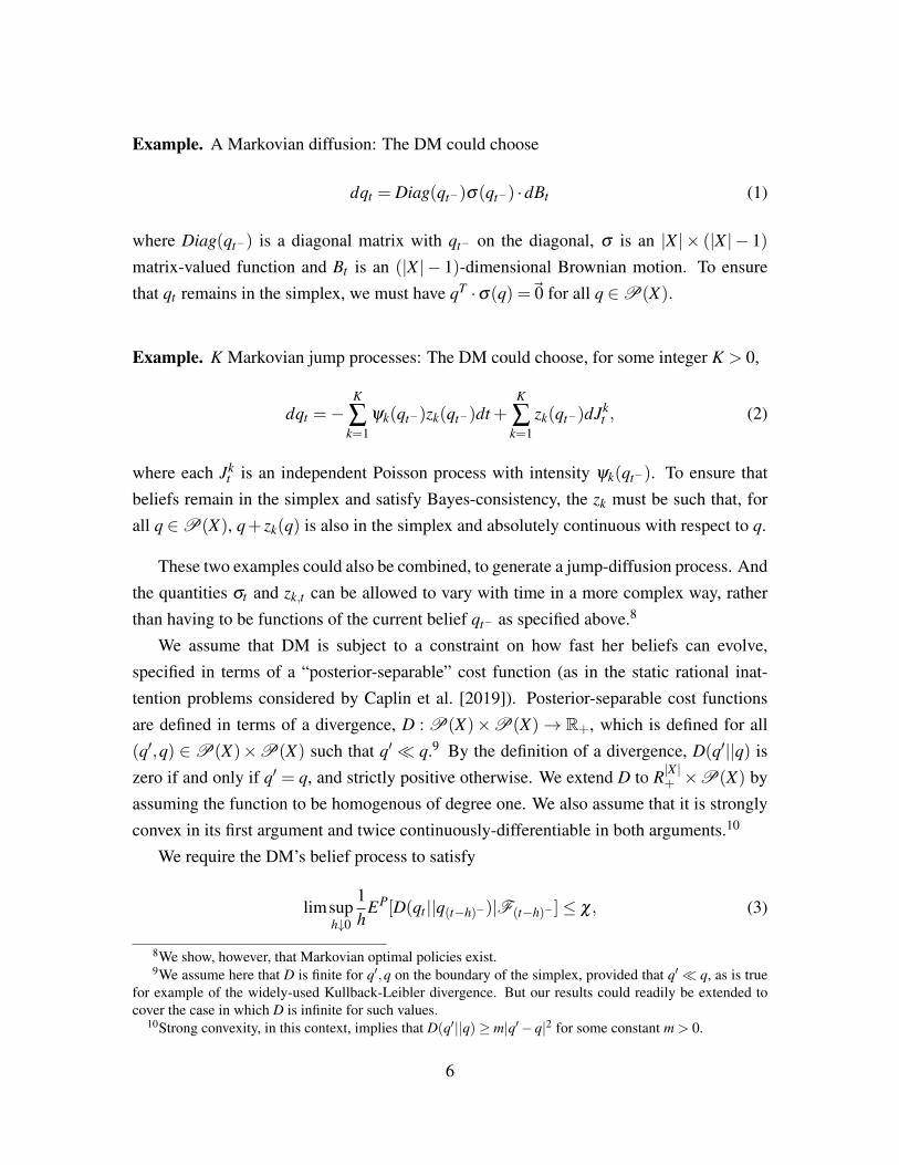
Example. A Markovian diffusion: The DM could choose

dqt = Diag(qt−)σ(qt−) ·dBt (1)

where Diag(qt−) is a diagonal matrix with qt− on the diagonal, σ is an |X | × (|X | − 1)matrix-valued function and Bt is an (|X | − 1)-dimensional Brownian motion. To ensurethat qt remains in the simplex, we must have qT ·σ(q) =~0 for all q ∈P(X).

Example. K Markovian jump processes: The DM could choose, for some integer K > 0,

dqt =−K

∑k=1

ψk(qt−)zk(qt−)dt +K

∑k=1

zk(qt−)dJkt , (2)

where each Jkt is an independent Poisson process with intensity ψk(qt−). To ensure that

beliefs remain in the simplex and satisfy Bayes-consistency, the zk must be such that, forall q ∈P(X), q+ zk(q) is also in the simplex and absolutely continuous with respect to q.

These two examples could also be combined, to generate a jump-diffusion process. Andthe quantities σt and zk,t can be allowed to vary with time in a more complex way, ratherthan having to be functions of the current belief qt− as specified above.8

We assume that DM is subject to a constraint on how fast her beliefs can evolve,specified in terms of a “posterior-separable” cost function (as in the static rational inat-tention problems considered by Caplin et al. [2019]). Posterior-separable cost functionsare defined in terms of a divergence, D : P(X)×P(X)→ R+, which is defined for all(q′,q) ∈P(X)×P(X) such that q′ q.9 By the definition of a divergence, D(q′||q) iszero if and only if q′ = q, and strictly positive otherwise. We extend D to R|X |+ ×P(X) byassuming the function to be homogenous of degree one. We also assume that it is stronglyconvex in its first argument and twice continuously-differentiable in both arguments.10

We require the DM’s belief process to satisfy

limsuph↓0

1h

EP[D(qt ||q(t−h)−)|F(t−h)−]≤ χ, (3)

8We show, however, that Markovian optimal policies exist.9We assume here that D is finite for q′,q on the boundary of the simplex, provided that q′ q, as is true

for example of the widely-used Kullback-Leibler divergence. But our results could readily be extended tocover the case in which D is infinite for such values.

10Strong convexity, in this context, implies that D(q′||q)≥ m|q′−q|2 for some constant m > 0.

6

where χ > 0 is a finite constant. This constraint can be understood as the continuous-timeanalog of requiring that Et−h[D(qt ||qt−h)]≤ χh in a discrete time model with time intervalh. Note also that in what follows, we will use the notation Et [·] to indicate EP[·|Ft ]. We il-lustrate the implications of this constraint in the context of our examples; these implicationsfollow from Ito’s lemma (for a proof, see Lemma 6 in the appendix).11

Example. A Markovian diffusion: in the context of the diffusion process (1), the constraint(3) requires that σ(q) satisfy the additional condition

12

tr[σ(q)T Diag(q)k(q)Diag(q)σ(q)]≤ χ (4)

for all q ∈P(X), where k(q) is an |X |× |X | matrix defined on the interior of the simplex,

kx,x′(qt−) =∂ 2D(q||qt−)

∂qx∂qx′|q=qt−

, (5)

and extended to the boundary by continuity.

Example. K Markovian jump processes: in the context of the jump process (2), the con-straint (3) requires that, for all q ∈P(X),

K

∑k=1

ψk(q)D(q+ zk(q)||q)≤ χ. (6)

We have specified the possible belief processes in this way to emphasize the connec-tion between our approach in continuous time and the standard, discrete-time approach torational inattention.12 The constraint (3) implies a tradeoff between more frequent but lessinformative movements in beliefs and rarer but larger movements in beliefs. Suppose thatthe DM would like her beliefs to follow a jump process of the kind specified in (2). TheDM can choose rare but informative signals (small ψk(q), large D(q+ zk(q)||q)) or morefrequent but less informative signals (larger ψk(q), smaller D(q+ zk(q)||q)). In fact, thereexists a limit in which jumps become very likely and very small (|zk| → 0,ψk → ∞) andthe stochastic process of beliefs and the information constraint for the jump process (2)

11Technical footnote: we require only that (3) hold for all (ω, t) ∈Ω×R+ outside of an evanescent set i.e.that the process qt is indistinguishable from a process for which the constraint holds everywhere.

12The working paper version of this paper (Hébert and Woodford [2019]) derives a version of ourcontinuous-time problem by considering the limit of a sequence of discrete-time problems.

7

converge to the stochastic process and constraint for a diffusion process (1). That is, theconstraint (3) ensures continuity between the cost of a continuous belief process and thecost of a belief process with very small jumps.

Let A denote the set of feasible policies (i.e. filtered probability spaces, stochasticprocesses for beliefs consistent with (3), and stopping times), and let ρ ≥ 0 denote theDM’s rate of time preference. We will assume that at least one of ρ or κ is strictly positive,so that the DM faces some cost of delay.

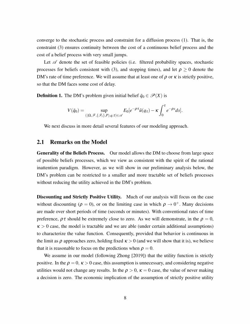
Definition 1. The DM’s problem given initial belief q0 ∈P(X) is

V (q0) = sup((Ω,F ,Ft,P),q,τ)∈A

E0[e−ρτ u(qτ)−κ

ˆτ

0e−ρsds].

We next discuss in more detail several features of our modeling approach.

2.1 Remarks on the Model

Generality of the Beliefs Process. Our model allows the DM to choose from large spaceof possible beliefs processes, which we view as consistent with the spirit of the rationalinattention paradigm. However, as we will show in our preliminary analysis below, theDM’s problem can be restricted to a smaller and more tractable set of beliefs processeswithout reducing the utility achieved in the DM’s problem.

Discounting and Strictly Positive Utility. Much of our analysis will focus on the casewithout discounting (ρ = 0), or on the limiting case in which ρ → 0+. Many decisionsare made over short periods of time (seconds or minutes). With conventional rates of timepreference, ρτ should be extremely close to zero. As we will demonstrate, in the ρ = 0,κ > 0 case, the model is tractable and we are able (under certain additional assumptions)to characterize the value function. Consequently, provided that behavior is continuous inthe limit as ρ approaches zero, holding fixed κ > 0 (and we will show that it is), we believethat it is reasonable to focus on the predictions when ρ = 0.

We assume in our model (following Zhong [2019]) that the utility function is strictlypositive. In the ρ = 0, κ > 0 case, this assumption is unnecessary, and considering negativeutilities would not change any results. In the ρ > 0, κ = 0 case, the value of never makinga decision is zero. The economic implication of the assumption of strictly positive utility

8

is that any action taken in finite time dominates never making a decision. This condition,which is stronger than necessary, ensures that optimal stopping times are well-behaved.

Information Constraints vs. Information Costs. We have described our model in termsof a constraint on rate at which information can be acquired. However, we would havereached identical results had we instead treated the cost of information as entering the utilityfunction. Both approaches are common in the rational inattention literature, and equivalentfor our purposes, although they make different predictions in certain settings (e.g. withrespect to the effect of “scaling up” the utility function u on behavior). In the working paperversion of this paper (Hébert and Woodford [2019]), we discussed both primal (constraints)and dual (utility costs) problems, and provided some equivalence results.

In the case of no discounting (ρ = 0), whether the information cost is treated as a utilitycost or constraint is irrelevant: the optimal policies are identical across the two cases. Thisproperty comes from the fact that the cost of delay is constant. In the case with discounting(ρ > 0), the cost of delay depends in part on the current level of the value function, whichgenerates variation in the amount of information acquired when information costs are utilitycosts, but not when information costs are constraints. Our results, however, are not sensitiveto the differences between the optimal policies in these two cases.

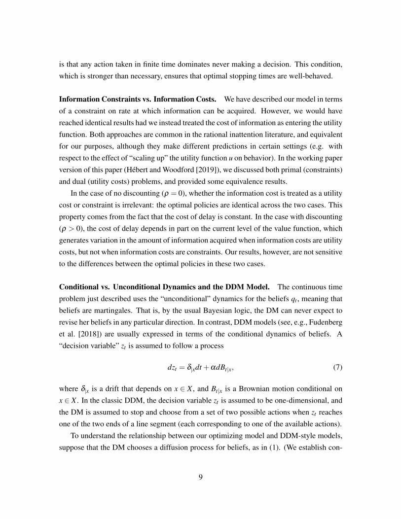
Conditional vs. Unconditional Dynamics and the DDM Model. The continuous timeproblem just described uses the “unconditional” dynamics for the beliefs qt , meaning thatbeliefs are martingales. That is, by the usual Bayesian logic, the DM can never expect torevise her beliefs in any particular direction. In contrast, DDM models (see, e.g., Fudenberget al. [2018]) are usually expressed in terms of the conditional dynamics of beliefs. A“decision variable” zt is assumed to follow a process

dzt = δ|xdt +αdBt|x, (7)

where δ|x is a drift that depends on x ∈ X , and Bt|x is a Brownian motion conditional onx ∈ X . In the classic DDM, the decision variable zt is assumed to be one-dimensional, andthe DM is assumed to stop and choose from a set of two possible actions when zt reachesone of the two ends of a line segment (each corresponding to one of the available actions).

To understand the relationship between our optimizing model and DDM-style models,suppose that the DM chooses a diffusion process for beliefs, as in (1). (We establish con-

9

ditions below under which this will be optimal.) Conditional on the true state being x ∈ X ,the DM’s beliefs qt follow a diffusion of the form the process13

dqt = Diag(qt−)σ(qt−)σ(qt−)T ex dt + Diag(qt−)σ(qt−)dBt|x, (8)

where ex is a vector equal to one in the element corresponding to x and zero otherwise.Note that this implies that, if we write µt−|x for the drift rate of qt,x in (8),

µt−|x = eTx Diag(qt−)σ(qt−)σ(qt−)

T ex ≥ 0.

Thus, the DM will tend to assign more probability to the true state as evidence accumulates.Thus if the DM chooses the kind of gradual evidence accumulation described by (1),

the belief process qt in our model has properties similar to those posited for the “decisionvariable” zt in the DDM model: it is a diffusion process with a drift that depends on the truestate x, and an instantaneous variance that is independent of the state. Below, we establishconditions under which it will be optimal for the belief process to be a diffusion of thiskind. Moreover, we establish conditions under which, in the case of a choice between onlytwo possible actions, it is optimal for the DM in our model to choose a belief process thatdiffuses on a line until it reaches one of two stopping boundaries, as posited by the DDM.14

2.2 Preliminary Analysis

We begin by showing that optimal policies exist. A key concern is the possibility of se-quences of policies that involve increasingly frequent but small jumps and converge in thelimit to diffusions. In this case, the stochastic processes for beliefs will converge to a con-tinuous martingale, even though no martingale in the sequence is continuous. Nevertheless,the constraint in (3) is continuous in this limit, and the limiting policy is feasible.

Lemma 1. There exists a set of optimal policies in the DM’s problem.

Proof. See the appendix, section A.1.

13This expression follows from Bayes’ rule and the Girsanov theorem.14It is well known that optimal Bayesian decision making would imply a process of this kind in the special

case that (i) there are only two possible states x, so that the posterior necessarily moves on a line, and(ii) the only possible kind of information sampling is observation of a particular Brownian motion withstate-contingent drift, so that the DM’s only decision is when to stop observing and choose an action, as inFudenberg et al. [2018]. The novelty of our result is that we allow a flexible choice of the kind of informationthat is sampled, subject to (3), and that our result applies regardless of the number of states in X .

10

This result ensures that the questions we hope to address, such as when optimal policiesinvolve jumps or diffusions, in fact have answers.

Next we show that the value function for our problem must satisfy a Hamilton-Jacobi-Bellman (HJB) equation. This is not trivial, because in our context, the value functionneed not be twice continuously-differentiable, and consequently the HJB equation cannotbe derived in the usual fashion. We take an alternative approach using viscosity techniquesto show that the value function is once continuously-differentiable, and that it is a solutionto an HJB equation of a simpler problem.

To simplify our notation, we extend the definition of V to the set of positive measures(R|X |+ ) by assuming homogeneity of degree one, and define the gradient of V , ∇V , in theusual way. Also, for any belief q ∈P(X), let Q(q) be the subset of P(X) consisting of allbeliefs q′ such that q′ 6= q,q′ q (the set for which D(q′||q) is defined and non-zero).

Proposition 1. Let V (q) be the value function that solves the DM’s problem (Definition 1).

This value function is continuously differentiable on the interior of P(X) and the interior

of each face of P(X), and satisfies, for all q ∈P(X),

max supq′∈Q(q)

V (q′)−V (q)− (q′−q)T ·∇V (q)D(q′||q)

−ρV (q)−κ, u(q)−V (q) = 0.

Proof. See the appendix, section A.3

This is the HJB equation of a restricted version of our problem in which the DM isconstrained not to diffuse and to jump to only one destination (a process of the form (2)with K = 1). That is, imposing such a restriction on the belief dynamics does not reduce theDM’s value function. Note that optimal policies may not exist in this restricted problem, ifit is in fact strictly optimal to diffuse in the original problem; in such a case, a sequence of“pure jump” policies involving ever-smaller and more frequent jumps achieves the supre-mum. The useful general characterization of the value function in Proposition 1 allows usto establish further properties of optimal belief dynamics in a variety of special cases.

3 Preferences for Gradual and Discrete Learning

We next study the relationship between properties of the divergence D and properties ofbeliefs under optimal policies. We consider two cases: when there is a “preference forgradual learning” and when there is a “preference for discrete learning,” terms we define

11

below. These two classes of divergences lead, respectively, to beliefs that move in smallincrements and beliefs that move in large increments. In the case of zero discounting, apreference for gradual learning leads to beliefs that diffuse, as in the DDM model.

3.1 Gradual Learning

We begin by defining what we call a “preference for gradual learning.” This conditiondescribes the relative costs of learning via jumps in beliefs vs. continuously diffusingbeliefs, which are governed by the properties of the divergence D.

Definition 2. The divergence D exhibits a “preference for gradual learning” if, for allq,q′ ∈P(X) with q′ q,

D(q′||q)≥ (q′−q)T · (ˆ 1

0(1− s)k(sq′+(1− s)q)ds) · (q′−q). (9)

This preference is “strict” if the inequality is strict for all q′ 6= q, and is “strong” if, for someδ > 0 and some m > 0,

D(q′||q)≥ (1+m|q′−q|δ )(q′−q)T · (ˆ 1

0(1− s)k(sq′+(1− s)q)ds) · (q′−q). (10)

Note that, to second order, D(q′||q) = (q′−q)T k(q)(q′−q)+o(|q′−q|2). A preferencefor gradual learning requires that the higher-than-second-order terms be positive, a strictpreference requires that they be strictly positive as q′ approaches q, and a strong preferencerequires that they be of order |q′−q|2+δ .

One special case of particular interest involves Bregman divergences (such as the Kullback-Leibler divergence commonly used in the rational inattention literature). A Bregman diver-gence can be written, using some convex function H : P(X)→ R, as

DH(q′||q) = H(q′)−H(q)− (q′−q)T ·∇H(q), (11)

where ∇H(q) denotes the gradient. For a Bregman divergence, k(q) is the Hessian of H(q),and (9) is an equality for all q,q′ ∈P(X).

Divergences exhibiting a (strict or strong) preference for gradual learning can be easily

12

constructed from Bregman divergences. Suppose that

D(q′||q) = f (DH(q′||q)),

where f : R+→R+ is a twice continuously-differentiable, strictly increasing, convex func-tion with f (0)= 0, f ′(0)= 1, and DH is a Bregman divergence. The Hessian of D evaluatedat q′ = q is the same as that of DH , and by convexity

D(q′||q)≥ DH(q′||q),

implying that D also exhibits a preference for gradual learning. This preference is strict iff (·) and H(·) are strictly convex, and strong if H(·) and f (·) are strongly convex.

We begin our analysis with a lemma, showing that the value function’s curvature islimited by the possibility of diffusing along a line. Note that this lemma holds regardlessof whether D exhibits a preference for gradual learning.

Lemma 2. For all q,q′ ∈P(X) such that q′ q and q′ 6= q,

V (q′)−V (q)− (q′−q) ·∇V (q)≤

(q′−q)T · (ˆ 1

0(1− s)χ−1(ρV (sq′+(1− s)q)+κ)(k(sq′+(1− s)q)ds) · (q′−q).


Lemma 2 and the HJB equation in Proposition 1 together show that the curvature ofthe value function (V (q′)−V (q)− (q′− q) ·∇V (q)) is limited by both the possibility ofdirectly jumping from q to q′ and the possibility of attempting to diffuse from q to q′. Inthe case of a strong preference for gradual learning, the bound arising from the possibilityof diffusing is tighter for sufficiently large values of |q′−q|. The intuition behind this resultcomes from a “race” between the strong preference for gradual learning of the divergence,which makes jumping as opposed to diffusing increasingly costly as |q′−q| becomes large,and the potentially increasing cost of delay under a diffusion policy (ρV (sq′+(1− s)q)

vs. ρV (q)). Because the value function is bounded, the cost of delay can increase only somuch, and consequently for |q′−q| sufficiently large, the diffusion bound must be tighterthan the direct jump bound.

13

Lemma 3. Let umax = maxq∈P(X) u(q) and umin = minq∈P(X) u(q). If D exhibits a strong

preference for gradual learning, then

V (q′)−V (q)− (q′−q)T ·∇V (q)D(q′||q)

< χ−1(ρV (q)+κ) (12)

for all q,q′ ∈P(X) such that q′ q, q′ 6= q, and

|q′−q|δ >ρ(umax−umin)

m(κ +ρumin).

Proof. By contradiction: suppose the reverse inequality holds for some q′ satisfying thiscondition. Then by Lemma 2 and the definition of a strong preference for gradual learning,

D(q′||q)1+m|q′−q|δ

(ρumax+κ)χ−1≥V (q′)−V (q)−(q′−q)·∇V (q)≥ χ−1(ρumin+κ)D(q′||q),

which yields ρ(umax−umin)κ+ρumin

≥ m|q′−q|δ , a contradiction.

A consequence of this result is that when D exhibits a strong preference for graduallearning, there exists an optimal policy such that the probability of a jump of size greaterthan (ρ(umax−umin)

m(κ+ρumin))δ−1

is zero.15

Proposition 2. Define ∆qt = qt − lims↑t qs and ∆Vt = V (qt)− lims↑t V (qs). If D exhibits a

strong preference for gradual learning, then there exists an optimal policy such that

Pr supt∈R+

|∆qt |> (ρ(umax−umin)

m(κ +ρumin))δ−1= 0,

and such that all jumps increase the value function (∆Vt ≥ 0, almost surely strictly wherever

|∆qt |> 0).


The optimal policy in this case features upward (in the sense of the value function)jumps and downward drift. The fact that jumps only increase and never decrease the valuefunction is a consequence of the exponential discounting. Exponential discounting can be

15We conjecture that a stronger result here is possible (at the expense of additional technicalities)– that theprobability of such large jumps is zero under any optimal policy.

14

thought of as a penalty for delay that is increasing in the current level of the value function.For this reason, drifting upward and jumping downward is sub-optimal, because the formercauses information to be acquired at a time when the cost of delay is high, and the latteracquires information at a time when the cost of delay is high rather than waiting for thecost of delay to decrease.16

In the particular case of no discounting (ρ = 0,κ > 0), we can reach stronger con-clusions. The sub-optimality of a jump, (12), must hold for all q′ 6= q. Consequently, anoptimal diffusion policy exists. The following proposition extends this result to the caseof a (possibly non-strong or non-strict) preference for gradual learning.17 Recall that thematrix-valued function k(q) is defined in (5).

Proposition 3. If ρ = 0 and D exhibits a preference for gradual learning, then V is a

viscosity solution (see e.g. Crandall et al. [1992]) to the HJB equation

max supσ∈R|X |×R|X |−1:qT σ=~0

tr[σT Diag(q)(∇2V (q)− κ

χk(q))Diag(q)σ ], u(q)−V (q)= 0,

(13)where ∇2V denotes the Hessian of V , and there exists an optimal policy such that qt is a

diffusion without jumps.


Under an additional assumption (described in the next section), a preference for graduallearning is not only sufficient but necessary for beliefs to follow a diffusion process in theρ = 0 case. In particular, we will demonstrate that if, for all utility functions, an optimalbelief process in the continuous time limit is a diffusion, then the divergence must exhibita preference for gradual learning. However, to make this statement, we must be able tocharacterize the belief dynamics, which we are able to do given an additional assumption.We therefore postpone our proof of necessity to the next section.18

Lastly, let us note that there is a kind of continuity between the ρ > 0 but small andρ = 0 cases (assuming κ > 0). As ρ converges towards zero, with a strong preference for

16This intuition is reminiscent of a related result in Zhong [2019], discussed below.17As before, to avoid technicalities, we do not prove a stronger claim that we conjecture holds: that in the

case of a strict preference for gradual learning and ρ = 0, all policies involve diffusions.18The difficulty of extending this result (without our additional assumption, or with ρ > 0) is as follows.

We know in these cases that if beliefs always diffuse or jump in small increments, then such behavior must bepreferable to larger jumps within the continuation region of a given problem. But because we cannot constructexplicit solutions in these cases, we cannot be certain that this preference holds on the entire simplex.

15

gradual learning, the magnitude of jumps becomes increasingly small, and in the limit nojumps occur. Let us note also a remarkable result from Zhong [2019], which shows thatwith ρ > 0, the optimal policy involves jumps outside of a nowhere-dense set. These tworesults are compatible: the jumps in this case are small but not infinitesimal.

Zhong [2019] also shows, in the particular case of ρ > 0 and Bregman divergence costs(equality in (9)), that the beliefs jump all the way to stopping points, a result we restatebelow. This is striking in light of proposition 3, which shows that with these same costsand ρ = 0, beliefs can follow a diffusion process. These results can be reconciled usingresults we will present in the next section: with Bregman divergence costs and ρ = 0, thereare optimal policies that generate both pure diffusion and pure-jump belief processes.

3.2 Discrete Learning

We next provide conditions under which the DM jumps immediately to stopping beliefs,as a contrast to our previous gradual learning results. We define what we call a “preferencefor discrete learning” if the divergence D satisfies a kind of “chain rule” inequality.19

Definition 3. The divergence D exhibits a “preference for discrete learning” if it satisfies,for all finite sets S, πs ∈P(S) and q,q′,qss∈S ∈P(X) such that ∑s∈S πsqs = q′ andq′ q,

D∗(q′||q)+∑s∈S

πsD∗(qs||q′)≥∑s∈S

πsD∗(qs||q). (14)

Here, S is an arbitrary a finite set; it is useful to think of each s∈ S as a signal realization,and to interpret qs as a set of posteriors consistent with a prior q′. If (14) holds, it ispreferable to jump from q directly to the posteriors qs instead to the prior q′.

Bregman divergences satisfy (14) with equality (a result that follows from the definition(11)). One might expect that other classes of cost functions also exhibit a preference fordiscrete learning. However, as the following lemma demonstrates, under our regularityassumptions,20 only the Bregman divergences exhibit a preference for discrete learning.

Lemma 4. The divergence D exhibits a preference for discrete learning if and only if D is

a Bregman divergence.19When this inequality holds with equality, the divergence is said to satisfy the chain rule property (Cover

and Thomas [2012]).20Our regularity assumptions are important here; it is possible that non-differentiable, non-Bregman diver-

gences exhibiting a preference for discrete learning exist.

16

Proof. See the appendix, section A.7. The proof builds on Banerjee et al. [2005].

Consequently, if D exhibits a preference for discrete learning, it also exhibits a (non-strict) preference for gradual learning. In contrast, many cost functions exhibit a strict orstrong preference for gradual learning and therefore do not exhibit a preference for discretelearning, and many others fall into neither category (e.g. if they have a strict preference forgradual learning in some parts of the parameter space and discrete learning in others).

If the cost function satisfies a preference for discrete learning, it its cheaper for theDM to jump to beliefs qs rather than visit the beliefs q′. Unsurprisingly, if this holdseverywhere, it leads to optimal policies that stop immediately after jumping. We first showin the case of ρ = 0 that an optimal policy always involves jumping into the stopping region.

Proposition 4. Define ∆qt = qt − lims↑t qs, and assume ρ = 0. If D exhibits a preference

for discrete learning, then there exists an optimal policy that does not diffuse and such that

if |∆qt |> 0, then t = τ (the DM stops immediately after any jump).

Proof. See the appendix, section A.8. This is proven using Proposition 7 below.

The statement of Proposition 4 shows that if D is a Bregman divergence, is without lossof generality to assume that the DM stops immediately after a jump in beliefs. But in thiscase, there is also an optimal policy that diffuses (Proposition 3). This observation impliesthat the solutions to the HJB equations in Propositions 1 and 3 must be identical, despiteone being written as controlling a diffusion process and the other a pure jump process. Werevisit this observation in the next section.

We next restate a result of Zhong [2019] (see appendix A.3 of that paper) that coversthe ρ > 0 case.21 With a preference for discrete learning, as with a preference for graduallearning, jumps will increase the value function. The intuition is essentially the same asthe gradual learning case, and comes from the observation that with discounting, delay isparticularly costly when the value function is high. However, unlike the gradual learningcase, in which jumps are of bounded size, with a preference for discrete learning jumps arealways immediately following by stopping. Zhong [2019] also shows that optimal policiesdo not involve diffusion (subject to some technical caveats).

Proposition 5. (Zhong [2019]) Define ∆qt = qt − lims↑t qs and ∆Vt =V (qt)− lims↑t V (qs)

and assume ρ > 0. If D exhibits a preference for discrete learning, then in any optimal

21The result from Zhong [2019] applies when κ = 0; but with ρ > 0, the κ > 0 problem is equivalent to aproblem in which the utility function is shifted upwards by κρ−1 and κ is set to zero (by Proposition 1).

17

policy, if |∆qt | > 0, then t = τ (the DM stops after jumping) and ∆Vt > 0 (jumps increase

the value function). In any optimal policy, diffusion occurs only on a nowhere-dense set.

Moving beyond the results of Zhong [2019], we provide the “only-if” result: if a diver-gence always results in large jumps and immediate stopping, then it must satisfy a prefer-ence for discrete learning. The intuition is that if it is always optimal to jump outside thecontinuation region, it cannot be less costly under the divergence D to jump to an inter-mediate point. Otherwise, there would be some utility function for which such behavior isoptimal. To formalize this result, we say that the beliefs process qt “does not diffuse” if thecontinuous part of the martingale qt has zero quadratic variation.22

Proposition 6. Define ∆qt = qt − lims↑t qs. Suppose the divergence D is such that, for all

action spaces A, strictly positive utility functions ua,x, and priors q0 ∈P(X), there exists

an optimal policy that does not diffuse on the interior of the continuation region outside of

a nowhere-dense set and such that |∆qt | > 0 implies t = τ (the DM stops after jumping).

Then D exhibits a preference for discrete learning (i.e. is a Bregman divergence).


Combining this result with Theorem 6, we have demonstrated that the jump-and-immediately-stop result of Zhong [2019] holds for all utility functions if and only if D is a Bregmandivergence. Such cases are knife-edge, in that if one uses instead any strongly convextransformation of the Bregman divergence, then the optimal policy will involve boundedjumps (by Proposition 2) that converge to diffusion processes as ρ becomes close to zero.

3.3 Gradual vs. Discrete Learning

We summarize the differences between gradual and discrete learning before proceeding.With ρ > 0 and a strong preference for gradual learning, the DM will optimally chooseto have beliefs that jump in small increments. In the limit as ρ → 0+, these jumps willbecome infinitesimal, and the DM will optimally choose to have beliefs that diffuse. Incontrast, with ρ > 0 and a preference for discrete learning, the DM will optimally choosehave beliefs that jump immediately into the stopping region. In the limit as ρ → 0+, thiswill continue to be case; however, when ρ = 0 and the DM has a preference for discretelearning, an optimal policy involving only diffusions also exists.

22See e.g. theorem 4.18 of chapter I of Jacod and Shiryaev [2013] on the decomposition of martingalesinto a continuous martingale and discontinuous martingale.

18

We interpret these results as follow. In the ρ→ 0+ limit, which we view as empiricallyrelevant (as most decision-making experiments involve small time periods), beliefs willeither jump or diffuse, depending on whether the divergence D exhibits a strong preferencefor gradual learning or a preference for discrete learning. However, the value functions inthese two cases might be identical. These results naturally lead to the question of whetherthese differences in belief dynamics lead to different predictions about the DM’s behavior.We explore this question in the next two sections.

4 The Equivalence of Static and Dynamic Models

In this section, we analyze the ρ = 0 continuous time model under a preference for graduallearning and a preference for discrete learning. The main result of this section is that,both with a preference for gradual learning and a preference for discrete learning (underan integrability assumption in the case of a preference for gradual learning), the valuefunction with ρ = 0 is equivalent to a static rational inattention problem with a uniformlyposterior-separable cost function (i.e. a cost function defined from a Bregman divergence,see Caplin et al. [2019] or (16) below). Moreover, any twice continuously-differentiableuniformly posterior-separable cost function can be justified through either of these routes.Our equivalence result extends to policies as well, in the sense that the joint distribution ofactions and states induced by optimal policies in the continuous time model is also optimalin the static model, and vice-versa.

This result has several implications. First, it demonstrates that both jump and diffusion-based models are tractable and that the value functions can be characterized without directlysolving the associated partial differential equation. Second, it provides a micro-foundationfor the uniformly posterior-separable cost functions that have been emphasized in the liter-ature. Third, it proves that the two approaches are equivalent in terms of the predicted jointdistribution of states x ∈ X and actions a ∈ A. That is, any joint distribution of (x,a) thatcould be observed under discrete learning could be observed under gradual learning.

On this last point, however, we do not mean to imply that the diffusion and jump pro-cesses are equivalent. Both of them endogenously will result in the same joint distributionof actions and states, but will have different predictions about the joint distribution of ac-tions, states, and stopping times. As a consequence, considering stopping times can helpdifferentiate the two models, and we consider this in the next section.

Our results in the case of gradual learning depend on an additional integrability assump-

19

tion that does not hold generically. Consequently, equivalence with static models holds forall cost functions with a preference for discrete learning but only some cost functions for apreference for gradual learning, and all cost functions with a preference for discrete learn-ing generate the same joint distribution of actions and states as some cost function with apreference for gradual learning, but the reverse is not true.

4.1 Gradual Learning

To prove our equivalence result, we restrict our attention to information-cost matrix func-tions that are “integrable,” in the sense described by the following assumption.23

Assumption 1. There exists a twice continuously-differentiable function H :R|X |+ →R such

that, for all q in the interior of the simplex,

k(q) = ∇2H(q), (15)

where ∇2H(q) denotes the Hessian of H evaluated at q and k(q) is define as in (5).

Any Bregman divergence has this property; as a result, the class of divergences sat-isfying this property includes the standard KL divergence and the “neighborhood-based”function that we introduce in Hébert and Woodford [forthcoming]. Our earlier examplesof divergences with a strong preference for gradual learning, which are not Bregman di-vergences themselves but were constructed by applying a convex function to a Bregmandivergence, also satisfy this property. In these cases, the H function is the function usedto define the Bregman divergence. This assumption is also automatically satisfied in thetwo state case, |X | = 2. However, this assumption imposes some restrictions if |X | > 2.It rules out, for example, the prior-invariant LLR cost functions of Pomatto et al. [2018](a hypothetical H would have asymmetric third-derivative cross-partials). We refer to thefunction H as the “entropy function,” for reasons that will become clear below. Note thatH(q) is convex, by the positive semi-definiteness of k(q), and homogenous of degree one.

The problem we are analyzing is the HJB equation of Proposition 3 (the problem withρ = 0 and a diffusion process for beliefs). We describe our equivalence result below.

23Mathematically, this assumption ensures that the integral´ 1

0 (q′− γ(s))T · k(γ(s)) · dγ(s)

ds ds is the same forall differentiable paths of integration γ : [0,1]→P(X) with γ(0) = q and γ(1) = q′. That is, the straight-linepath of integration used to define a preference for gradual learning (Definition 2) is without loss of generality.

20

Proposition 7. If ρ = 0, D exhibits a preference for gradual learning, and Assumption 1

holds, the value function is

V (q0) = maxπ∈P(A),qa∈P(X)a∈A

∑a∈A

∑x∈X

πaqa,xua,x−κ

χ∑a∈A

π(a)DH(qa||q0),

subject to the constraint that ∑a∈A π(a)qa = q0, where DH is the Bregman divergence asso-

ciated with the entropy function H that is defined by Assumption 1, and this value function

can be achieved by a pure diffusion process.

There exist maximizers π∗ and q∗a such that π∗ is the unconditional probability, in

the continuous time problem, of choosing a particular action, and q∗a, for all a such that

π∗(a)> 0, is the unique belief the DM will hold when stopping and choosing that action.

Proof. See the appendix, Section section A.10.

Let S be a set of possible signal realizations, and let p : X →P(S) be a “signal struc-ture” that defines the conditional distribution of signal realizations in each state x ∈ X .Taken as given a prior q0 ∈P(X), and let πs(p,q0) and qs(p,q0) denote the unconditionalsignal probabilities and posteriors, respectively, given the prior and signal structure. Ourcontinuous time problem is equivalent to a static rational inattention problem in which theDM chooses S and p, given a prior q0 ∈P(X), with a particular uniformly posterior-separable (UPS) cost function,

C(p,q0; S) =κ

χ∑s∈S

πs(p,q0)DH(qs(p,q0)||q0), (16)

and with the signal space S identified with the set of possible actions A. The equivalencebetween our (seemingly complex) continuous time model and this static model renders theformer tractable, both in the special cases in which analytic solutions to the static modelare available and computationally (because the static model is straightforward to studynumerically). The cost scalar κ

χparametrizes the tradeoff between stopping and acquiring

more information, which is governed by the rate at which information can be acquired (χ)and the cost of delay (κ).

The mutual information cost function proposed by Sims is one example of a UPS costfunction. In this case, the entropy function H is the negative of Shannon’s entropy, thecorresponding Bregman divergence is the Kullback-Leibler divergence, and the informa-tion cost defined by (16) is mutual information. Thus Proposition 7 provides a foundation

21

for the standard static rational inattention model, and hence for the same predictions re-garding stochastic choice as are obtained by Matêjka et al. [2015]. On the other hand,Proposition 7 also implies that other cost functions can also be justified. Indeed, any (twicecontinuously-differentiable) uniformly posterior-separable cost function (16) can be givensuch a justification, by choosing the k function defined by equation (15).

We conclude that all continuous time models with gradual learning that also satisfy ourintegrability condition are equivalent to a static model with a uniformly posterior-separablecost function, and that any such static model can be justified from some model with graduallearning. We next show that the same set of static models can be justified from a modelwith discrete learning. Before proceeding, however, we observe that this result allows us todemonstrate that a preference for gradual learning is necessary for beliefs to always resultin a diffusion process, provided that Assumption 1 holds.

Corollary 1. Assume ρ = 0. If, given a divergence D, Assumption 1 is satisfied and, for all

strictly positive utility functions ua,x, there exists an optimal policy such that beliefs follow

a diffusion process, then D exhibits a preference for gradual learning.


4.2 Discrete Learning

The result with a preference for discrete learning is an immediate corollary of Lemma 4and the preceding Proposition 7 (the result with gradual learning).

Corollary 2. Assume ρ = 0 and that D exhibits and preference for discrete learning (i.e.

is a Bregman divergence). Then the value function that solves the continuous time prob-

lem is the value function that solves the static rational inattention problem described in

Proposition 7, with D in the place of DH .

Proof. Immediate from Lemma 4, Proposition 3, and Proposition 7.

Given any uniformly posterior-separable cost function in a static rational inattentionmodel, by setting D equal to the Bregman divergence associated with that cost function,we can justify that static model as the result of a dynamic model with a preference fordiscrete learning. We therefore conclude that models with a preference for gradual learningsatisfying our integrability condition and models with a preference for discrete learningare indistinguishable from the perspective of their predictions about the joint distribution

22

of states and actions.24 In the next section, we begin to explore how information aboutstopping times can be used to distinguish the models.

5 Implications for Response Times

Because our model is dynamic, it makes predictions not only about the joint distribution ofactions and states, but also the length of time that should be taken to reach a decision, andhow this may vary depending on the action and the state. In the experimental literature onthe accuracy of perceptual judgments, it is common to record the time taken for a subject torespond along with the response, as this is considered to give important information aboutthe nature of the decision process (e.g., Ratcliff and Rouder [1998]).

Here we propose that data on response times can in principle be used to discriminatebetween alternative information-cost specifications. We will show that divergences thatare equivalent in the sense of implying the same state-contingent choice probabilities —and hence the same value function in the case that discounting is negligible — neverthelessmake different predictions about the stopping time conditional on taking a particular action.Consequently, data on response times can inform us about whether there is a preference forgradual learning or for learning through discrete jumps. Interestingly, it is possible todistinguish between these two hypotheses even when (as in the problems considered here)actions are taken only infrequently.25

5.1 The Two-Action Case

To illustrate this possibility, we consider a simple example, in which there are two possibleactions (A = L,R). We will consider the ρ → 0+ limit and impose Assumption 1. Wecompare behavior with a divergence D exhibiting a strict preference for gradual learning tothe behavior generated by the Bregman divergence DH (as defined in Proposition 7), whichexhibits a preference for discrete learning. By Proposition 7, these two divergences willgenerate identical value functions V (q); but with a strict preference for gradual learning,beliefs will diffuse, whereas with a preference for discrete learning beliefs will jump.

24In situations in which the static rational inattention problem does not itself have a unique solution, wehave not ruled out the possibility that the models with discrete and gradual learning will make differentpredictions. However, we have no reason to believe this is the case.

25It would obviously be easier to tell whether beliefs evolve continuously or in discrete jumps in a casewhere the DM is required to continuously adjust some response variable that can provide an indicator of hercurrent state of belief.

23

With both of these divergences, by Proposition 7, beliefs will move on a line; this isa consequence of the “locally invariant posteriors” property of Caplin et al. [2019] andthe fact that there are only two actions. Let q∗L and q∗R be the optimal posteriors given theprior q0 in the static rational inattention problem described in Proposition 7, and let π∗Lbe the optimal unconditional probability of action L. We will assume some information isacquired, which is to say q∗L 6= q∗R 6= q0, and that all of these beliefs are on the interior ofthe simplex (to avoid technicalities). Under the optimal policy, beliefs will move (eitherdiffusing or jumping/drifting) on the line segment connecting q∗L and q∗R in the simplex,which necessarily runs through q0.

For this reason, it is convenient in the two-action case to express the dynamics of beliefsin terms of the state variable πL,t ∈ [0,1], which corresponds to the beliefs

qt = q(πL,t) ≡ q∗R +πL,t(q∗L−q∗R), (17)

with πL,0 = π∗L . When πL,t reaches one, the DM chooses L; when πL,t reaches zero, theDM chooses R. Our interest is in characterizing the conditional (on the true state x ∈ X)likelihood of stopping and choosing L or R at each time t.

Before proceeding, let us observe from Proposition 7 that the value function (in termsof the state variable πL,t) can be written as

V (πL,t) = πL,tVL +(1−πL,t)VR +κ

χH(q(πL,t)),

with VL =∑x∈X q∗L,xuL,x− κ

χH(q∗L) and VR =∑x∈X q∗R,xuR,x− κ

χH(q∗R). It follows by the strict

convexity of H(q) and the linearity of q(πL) that V (πL,t) is strictly convex on πL,t ∈ [0,1].As a consequence of this convexity, there are three possible shapes of the value functionV (πL,t): it could be increasing on [0,1], decreasing on [0,1], or decreasing on [0, πL) andincreasing on (πL,1] for some πL ∈ (0,1). In the first two of these cases, we will say πL = 0and πL = 1, respectively; thus in each case, πL is the value of πL at which V (πL) reaches itsminimum. We will show below that the shape of the value function is closely related to theproperties of the stopping time distribution in the case of a preference for discrete learning.

5.2 Distributions of Stopping Times

We begin by introducing some notation with which to describe our models’ predictionsregarding the distribution of observed response times. For any time τ, let Fx

a (τ) be the

24

cumulative probability of a decision a by time τ, conditional on the state being x. Forthe state x, and either action a, this is a right-continuous non-decreasing function, witha maximum equal to the overall probability of choosing a in state x. The sum Fx(τ) =

FxL (τ)+Fx

R(τ) is the cumulative distribution function of decision times when the state is x.It will be useful to state our theoretical predictions, not in terms of these distributions

for the decision time τ , but rather in terms of corresponding distributions for the response-time quantile τ. (The quantile τ of the response time τ is the fraction of all responses inthat state for which the response time is no greater than τ .) This has two key advantages.First, it allows us to state predictions that are independent of time units. The state- andresponse-contingent distributions for τ depend on the values of both κ and χ; instead, thepredicted distributions for τ depend only on their ratio.

Second, the response time observed in a laboratory experiment should not be identifiedwith the decision time τ in our theoretical model. Instead, empirical estimation of stochas-tic models like the DDM always interprets the measured response time as an observationof t0 + τ , where t0 (the “non-decision time,” NDT) is a positive constant to be estimated.26

The NDT may represent an unavoidable time lag between the experimenter’s presentationof a stimulus to the subject and the beginning of the evidence-accumulation process, or alag between the time τ at which the latent decision variable first reaches a stopping regionand the subject’s overt response. Predictions for the distributions of response-time quan-tiles τ are instead independent of the value of t0, as long as we assume that the NDT is aconstant (or more precisely, that its variance is vanishingly small, as discussed below).

For any quantile 0≤ τ ≤ 1, let Gxa(τ) be the fraction of all decisions in state x for which

the decision is a and the response-time quantile is no greater than τ . In the case of any τ

such that τ = Fx(τ) for some τ, we define, for either action a,

Gxa(τ) = Fx

a (τ). (18)

In some cases, however, the theoretical distribution of decision times τ has an atom atsome particular decision time τ . In this case, there is a jump in the c.d.f. at this point,Fx(τ−) = τ1 < τ2 = Fx(τ), which raises a question as to how Gx

a(τ) should be definedfor quantiles τ1 ≤ τ < τ2.

Let us suppose that, rather than a constant, the NDT on each trial is an independent

26For example, in Ratcliff and Rouder [1998] and Wagenmakers et al. [2007] this parameter is denoted Ter,while in Clithero [2018] it is written as ndt.

25

draw from a distribution with mean t0, and a continuous distribution (albeit one with avanishingly small variance).27 The c.d.f. of the distribution of observed response times(counting the NDT) will then be continuous but steep around the value t0 + τ. We can thendefine Gx

a(τ) for all τ using (18), and define, in the case of an atom at τ ,

Gxa(τ) = Fx

a (τ−) +(

τ− τ1

τ2− τ1

)(Fx

a (τ)−Fxa (τ−)) (19)

for all quantiles τa ≤ τ ≤ τ2. This definition preserves the property that each Gxa(τ) is a

non-decreasing function and that ∑a∈A Gxa(τ) = τ .

The empirical correlate of the functions Gxa(τ) can be computed using an experimental

dataset in which on each trial, the true state x, the response a, and the response time havebeen recorded. An especially interesting feature of these functions is what they implyabout how the relative probability of an L response as opposed to an R response varieswith the rapidity of the decision (early decisions versus late decisions, as measured by theresponse-time quantile τ). For each state-response pair (x,a), let us define gx

a(τ) as theright derivative of the function Gx

a(τ); we must have

gxa(τ) ≥ 0, gx

L(τ)+gxR(τ) = 1

for each quantile τ. The relative probability of an L response, conditional on state x, is thengiven by gx

L(τ). In the discussion below, we focus on the predicted shapes of gxL(τ).

5.3 Response Times with a Preference for Discrete Learning

In the case of a preference for discrete learning, the functions gxL(τ) are simple to describe.

In the previous sections, we have presented two relevant theoretical results. First, as dis-cussed above, beliefs will drift on a line segment in the simplex, until jumping to eitherq∗L or q∗R. Second, as emphasized by Zhong [2019], jumps must always increase the valuefunction, and the drift of beliefs will reduce the value function.28

Suppose, to simplify the exposition, that the minimum of the value function on the linesegment, V (πL), occurs at some πL < π∗L. For any πL,t > πL, the optimal policy is to jump

27We assume that the random NDT on any given experimental trial is independent of both the true state xand the sequence of evidence collected on that trial, and hence also independent of the decision that is made.

28The fact that the drift of beliefs will reduce the value function follows by applying the envelope theoremto the HJB equation of Proposition 1; see Zhong [2019].

26

towards πL,t = 1 with the maximum possible intensity and drift downwards. Eventually,πL,t will drift downwards and equal πL, at which point the DM will randomize betweenjumping to πL,t = 1 and πL,t = 0 with unconditional probabilities πL and (1− πL). In theparticular case of an upward-sloping value function (πL = 0), the DM will choose R withcertainty after reaching πL.

Regardless of the state, in the absence of a jump, πL,t will reach πL at a predictabletime, as beliefs drift downwards at a rate determined by the constraint (6),

µ(πL,t) = −χ(1−πL,t)

DH(q∗L||q(πL,t)).

Let τ be the time at which πL,t = πL in the absence of a jump.The unconditional likelihood of a jump prior to that time is determined by the constraint

(6); the conditional likelihood is then pinned down by Bayes’ rule. Suppose that the truestate is x, and let q = q(πL) be the beliefs the DM will hold if there has been no jump beforethe time τ . By Bayes’ rule, if her posterior must be qL conditional on jumping before timeτ , the probability of such a jump must satisfy

Prsupt∈[0,τ) |∆πL,t |> 0 |xPrsupt∈[0,τ) |∆πL,t |> 0

=q∗L,xq0,x

.

Moreover, by the martingale property of the unconditional belief process,

Pr supt∈[0,τ)

|∆πL,t |> 0q∗L,x + (1−Pr supt∈[0,τ)

|∆πL,t |> 0)qx = q0,x,

which yields

τx = Pr sup

t∈[0,τ)|∆πL,t |> 0|x =

q∗L,xq0,x

(q0,x− qx

q∗L,x− qx) =

q∗L,xqx(π∗L)

π∗L− πL

1− πL.

Intuitively, the likelihood of a jump conditional on x increases as the relative likelihood ofL given x increases. We can now observe that Prsupt∈[0,τ) |∆πL,t | > 0|x = τx is also thelikelihood of a decision before time τ . Consequently, the quantile at which πL,t = πL is τx,and gx

L(τ) = 1 for all τ < τx.After time τ, πL,t = πL until a jump occurs, and the relative likelihoods of jumping to

L and R are constant over time. Consequently, gxL(τ) is constant on τ ≥ τx, and determined

27

again by Bayes’ rule:

gxL(τ) =

q∗L,xqx

(qx−q∗R,x

q∗L,x−q∗R,x) =

πLq∗L,xqx(πL)

.

We thus obtain strong predictions about the functional form for gxL(τ): it is equal to

one for all τ < τx and constant for τ ≥ τx. States in which L is more likely (q∗L,xq∗R,x

larger)feature larger quantiles τx and higher values of gx

L(τ) for τ ≥ τx. Note that if we had insteadassumed π∗L < πL, we would reach similar conclusions with the roles of R and L reversed.

Figure 1 below illustrates these results. The first row considers the case of a symmetricvalue function, πL = 1

2 , the second an asymmetric case in which πL ∈ (0, 12), and the third

the case of a monotonically increasing value function (πL = 0). The first column plots thevalue function. The second column considers gG

L (τ) for a state G with q∗L,G > q∗R,G, and thethird column considers gB

L(τ) for a state B with q∗L,B < q∗R,B.We obtain even stronger predictions in the case that H is the Shannon entropy func-

tion, H(q) = ∑x qx lnqx, as assumed in many models of rational inattention following Sims[2010]. In this case, it is well-known that in the solution to the static rational inattentionproblem, the optimal information structure does not distinguish between states except tothe extent that the difference between them is payoff-relevant.29 For example, supposethat, as in many perceptual experiments, the reward ua,x for a particular response a in astate x (say, when a stimulus of type x is presented) depends only on whether a was the“correct” or “incorrect” response in that state, and let Xa be the subset of states for whicha is the correct response. Then because the utility differential uL,x−uR,x is the same for allstates x ∈ XL, it follows that q∗L,x/q∗R,x will be the same for every state x ∈ XL; and similarlyfor every state x ∈ XR. It then follows from our formulas above that both τx and gx

L (theconstant value for all τ ≥ τx) will be the same quantities for all x ∈ XL (“G states”), andwill similarly be the same quantities for all x ∈ XR (“B states”). Thus there will only be twofunctions gx

L(τ), the two functions shown as gGL (τ) and gB

L(τ) in Figure 1.The numerical examples shown in Figure 1 are calculated for an example of this kind.

H(q) is Shannon entropy, and ua,x depends only on whether x belongs to XL or XR (so thatwe can write ua,G in the case of a “G state” and ua,B in the case of a “B state”). In the top row(Case I), we further assume that the reward depends only on whether a response is corrector not (so that uL,G = uR,B > uR,G = uL,B). In this case, the symmetry of the problem resultsin a symmetric value function, as shown, with πL = 1/2. If we write q∗a,G = ∑x∈XL q∗a,x for

29This follows from the property that Caplin et al. [2019] call “invariance under compression.”

28

0 1 0 1

0

1

0 1

0

1

0 1 0 1

0

1

0 1

0

1

1 0 1

0

1

0 1

0

1

Figure 1: Predicted response-time distributions with a preference for discrete learning.Each row shows the value function V (πL), the function gx

L(τ) for states x in which L is thecorrect response (“G states”), and the function gx

L(τ) for states x in which R is the correctresponse (“B states”), under a particular assumption about the relative payoffs in G and Bstates. In the first row (Case I), the rewards for correct or incorrect responses are the samein G and B states; in the lower rows, the utilities associated with B states are made progres-sively lower relative those associated with G states. In all numerical calculations shown inthis figure, H(q) is assumed to be the Shannon entropy function. Information costs are pa-rameterized so that the predicted accuracy rate (PrL|G= PrR|B) is a = 0.84, and thefigures are drawn for the case of a prior q0,G = 0.75. These parameter choices are matchthe experimental data in Figure 3, but are also arbitrary, in the sense that the qualitativerelationships illustrated in the graph will hold regardless of these choices, provided that theprior implies that πL < π∗L < 1.

29

the probability of a G state under the posterior q∗a, and similarly q∗a,B for the probability ofa B state, then the symmetry of the problem also implies that q∗L,G = q∗R,B, a quantity thatwe denote a (the predicted overall fraction of correct responses). Then since we must have

q∗L,xq∗R,x

=q∗L,Gq∗R,G

=a

1−a∀x ∈ XL,

q∗L,xq∗R,x

=q∗L,Bq∗R,B

=1−a

a∀x ∈ XR,

the gradient of H (and hence the derivative of V (πL)) at each of the stopping posteriors iscompletely determined by the value of a. Thus the value of a determines the value functionV (πL), up to an additive constant. The value functions shown in Figure 1 assume thata = 0.84, the average accuracy rate in the experimental data shown in Figure 3.

In the second and third rows, we continue to assume the same utility differential be-tween the correct and incorrect responses in any state as in the top row: uL,G− uR,G =

uR,B−uL,B = ∆ > 0. However, we no longer assume that the reward for a correct responseis the same in G and B states. If we let uL,G− uR,B = uR,G− uL,B = δ , then δ = 0 cor-responds to Case I, shown in the top row. If instead 0 < δ < ∆, we have an asymmetricvalue function and 0 < πL < 1/2 (Case II), as shown in the second row of the figure. (Thenumerical solution shown in the second row is for δ = ∆/2.) Finally, if δ ≥ ∆, the valuefunction is monotonically increasing and πL = 0 (Case III), as shown in the bottom row.(The numerical solution shown is for δ = ∆.) We obtain similarly asymmetric solutions ifδ < 0, but with the roles of states G and B reversed.

The functions gxL(τ) shown in the other two panels of each row depend only on the

accuracy rate a and the values of πL, and π∗L (which depends on the prior). In the casesshown in Figure 1, we assume a prior under which G states are more likely than B states,and let the prior probability of some G state be q0,G = 0.75 (matching the experiment ofKelly et al. [2021], discussed below); this corresponds to π∗L ≈ 0.87.30

The result that the function gxL(τ) for any state x is necessarily one of the two functions

shown in Figure 1 depends on the special assumption that H(q) corresponds to Shannonentropy. However, if we assume that there are only two states (that is, that it is possible tocollect information directly about whether L or R is the correct response), then the numeri-cal solution for the functions gx

L(τ) for the two states x = G,B does not depend on any de-tails of the function H(q), apart from a symmetry assumption: that H(qG,qB) = H(qB,qG).

30If instead we were to assume that B states were more likely ex ante and that q0,B = 0.75, the functiongB

L(τ) would look like the function gGL (τ) shown in Figure 1, and the function gG

L (τ) would look like thefunction gB

L(τ) shown in Figure 1; hence we do not display additional figures for this case.

30

Under this assumption, the numerical values assumed for a, πL, and q0,G again completelydetermine the numerical specification of the functions gG

L (τ) and gBL(τ), and will exactly

match the ones shown in Figure 1.

5.4 Response Times with Gradual Learning and the DDM Model

Let us now consider instead the dynamics of the belief state πL,t , conditional on the truestate being x∈X , under a strict preference for gradual learning. Note first that the constraintfor a diffusion process, (4), will bind in any solution to the HJB equation (13). Becausediffusion takes place on a line (17), the unconditional belief dynamics are of the form

dqt = (q∗L−q∗R)σ(πL,t)dBt ,

where σ(πL) is scalar-valued and dBt is a one-dimensional Brownian motion. The con-straint (4) implies that

σ(πL,t)2 =

2χ

(q∗L−q∗R)T ·∇2H(q(πL,t)) · (q∗L−q∗R).

It then follows from (8) that the conditional dynamics of beliefs will be given by

dqt = (q∗L−q∗R)q∗L,x−q∗R,x

qt,xσ(πL,t)

2dt + (q∗L−q∗R)σ(πL,t)dBt|x,

conditional on any true state x. From this, we can derive the conditional dynamics for theunivariate belief state πL,t :

dπL,t =q∗L,x−q∗R,xqx(πL,t)

σ(πL,t)2dt + σ(πL,t)dBt|x. (20)

This process resembles the conditional beliefs process of a DDM in several respects.The state variable πL,t diffuses until reaching one of two fixed boundaries (zero or one),which correspond to the two action choices. States for which L is relatively more likely(

q∗L,xq∗R,x

positive) feature upward drift, and the strength of this drift is stronger in states forwhich the relatively probability of choosing L is higher. The only difference between thesedynamics and those of the standard DDM is that in general, neither the drift term nor thevariance term in (20) is constant.

However, under a particular assumption about information costs, the belief dynamics

31

implied by our model with a strict preference for gradual learning are exactly like thoseassumed in the standard DDM. Let us suppose that there are only two states, G and B, sothat the posterior can be represented by a single real number, qt,G, and the unconditionalbelief dynamics (until a decision is made) are of the form dqt,G = σ(qt,G)dBt , where σ(qG)

is a scalar. And suppose that instead of the Shannon entropy function, H(q) is what Bloedeland Zhong [2020] call a “total information” (TI) cost function:31

H(q) = (qG−qB)(ln(qG)− ln(qB)).

The maximum rate of information accumulation consistent with (4) is then given by

σ(qG) =√

2χqG(1−qG),

from which it follows, using (8), that the state-contingent belief dynamics are of the form

dqt,G = µx(qt,G)dt + σ(qt,G)dBt|x (21)

for x = G,B, where

µG(qG) = 2χqG(1−qG)2, µB(qG) = −2χq2

G(1−qG).

Since πL,t is a linear transformation of qt,G, the dynamics of the belief state πL,t stillhave a non-constant drift and instantaneous variance in this case. But suppose that weinstead parameterize the belief state by the posterior log odds, zt = ln(qt,G/qt,B). The isjust a smooth nonlinear transformation zt = Z(qt,G) of the posterior probability of state G;we can then use Ito’s lemma together with (21) to show that the state-contingent dynamicsof this variable are given by

dzt = χdt +√

2χdBt|G, dzt = −χdt +√

2χdBt|B.

These are just the kind of dynamics postulated in the standard DDM, with the differencebetween the drifts associated with the two states determined by the information boundχ. A decision will be made when the variable zt first reaches one or the other of twostopping values z∗a, which are just the log-odds transformations of the stopping posteriors

31Desirable properties of this alternative to the Shannon measure of information costs are also discussed inHébert and Woodford [forthcoming].

32

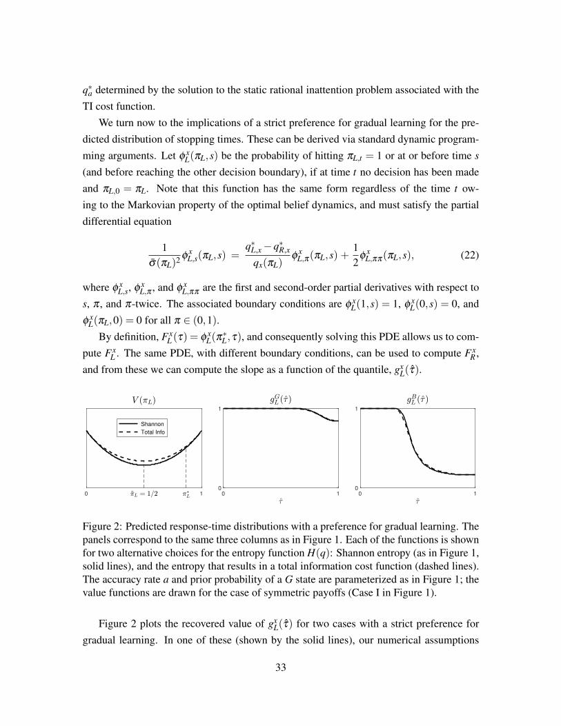
q∗a determined by the solution to the static rational inattention problem associated with theTI cost function.

We turn now to the implications of a strict preference for gradual learning for the pre-dicted distribution of stopping times. These can be derived via standard dynamic program-ming arguments. Let φ x

L(πL,s) be the probability of hitting πL,t = 1 or at or before time s

(and before reaching the other decision boundary), if at time t no decision has been madeand πL,0 = πL. Note that this function has the same form regardless of the time t ow-ing to the Markovian property of the optimal belief dynamics, and must satisfy the partialdifferential equation

1σ(πL)2 φ

xL,s(πL,s) =

q∗L,x−q∗R,xqx(πL)

φxL,π(πL,s) +

12

φxL,ππ(πL,s), (22)

where φ xL,s, φ x

L,π , and φ xL,ππ

are the first and second-order partial derivatives with respect tos, π , and π-twice. The associated boundary conditions are φ x

L(1,s) = 1, φ xL(0,s) = 0, and

φ xL(πL,0) = 0 for all π ∈ (0,1).

By definition, FxL (τ) = φ x

L(π∗L,τ), and consequently solving this PDE allows us to com-

pute FxL . The same PDE, with different boundary conditions, can be used to compute Fx

R ,and from these we can compute the slope as a function of the quantile, gx

L(τ).

0 1

Shannon

Total Info

0 10

1

0 10

1

Figure 2: Predicted response-time distributions with a preference for gradual learning. Thepanels correspond to the same three columns as in Figure 1. Each of the functions is shownfor two alternative choices for the entropy function H(q): Shannon entropy (as in Figure 1,solid lines), and the entropy that results in a total information cost function (dashed lines).The accuracy rate a and prior probability of a G state are parameterized as in Figure 1; thevalue functions are drawn for the case of symmetric payoffs (Case I in Figure 1).

Figure 2 plots the recovered value of gxL(τ) for two cases with a strict preference for

gradual learning. In one of these (shown by the solid lines), our numerical assumptions

33

are the same as in the first row of Figure 1, except that we now assume a strict preferencefor gradual learning. In particular, we again assume a function H(q) given by Shannonentropy; we assume that rewards depend only on whether the DM’s response is correct (sothat the value function is symmetric); and we assume the same numerical values for a andq0,G as in Figure 1. We show the figures only for the symmetric case (Case I) from Figure1, because as just explained, the utilities enter into the calculation of the functions gx

L(τ) inthe case of a strict preference for gradual learning only through their effect on the valuesof the stopping posteriors q∗a. Since the stopping posteriors are unaffected by a change inthe value of δ (holding fixed the utility differential ∆), the predicted functions gx

L(τ) undera strict preference for gradual learning will be the same in all three of the cases shown inFigure 1; hence we show only a single row in Figure 2.

As explained earlier, in the limit as ρ→ 0+, the value function is the same in the case ofa preference for gradual learning (PGL) as in the case of a preference for discrete learning(PDL); hence in the case of the cost function based on Shannon entropy (shown by thesolid line), the value function shown in Figure 2 is identical to the one shown in the upperleft panel of Figure 1. The dashed line shows the corresponding value function in the caseof a two-state model with the “total information” cost function discussed above. In thisalternative case, the model is again parameterized so as to imply the same values for a andq0,G as in the Shannon case (and as in Figure 1), and the value function is again shownfor the symmetric case (Case I in Figure 1). In the PDL model, the functions gx

L(τ) wouldcontinue in this alternative case to be the ones shown in the top row of Figure 1, as discussedabove. In the case of a strict preference for gradual learning, instead, the functions gx

L(τ)

are slightly different in the case of the total information cost function than in the case ofthe Shannon cost function. This is because in the PGL case the local curvature of thevalue function matters for the belief dynamics, and this is slightly different for the two costfunctions, as shown in the left panel of Figure 2.

Nonetheless, there are not large quantitative differences between the distributions ofresponse times implied by the two alternative cost functions, when these are parameterizedto imply the same accuracy rate a. Since the belief dynamics and stopping times impliedby the PGL model with the total information cost are identical to those of a particularparameterization of the DDM, we see that the distributions of response times implied bythe PGL model in either case are similar to those implied by the DDM. The differencesbetween the predictions of either version of the PGL model and the predictions for thePDL case are instead more notable.

34

5.5 Discriminating Between Discrete and Gradual Learning

A first important difference between the predictions of the discrete learning model andthose of the gradual learning model concerns the effects of varying the parameter δ inFigure 1. In the gradual learning model, transformations of the utility function that shiftutilities in a state contingent (but not action-contingent) fashion have no effect on behavior.To see this, suppose we shift the utility function ua,x to some u′a,x = ua,x + vx. It is im-mediately, from Proposition 7, that the value function will be shifted by ∑x∈X qxvx for anyq∈P(X). However, this will have no effect on behavior, as the level and slope of the valuefunction did not enter our analysis above of the case of gradual learning; only the secondderivatives of the value function at each point matter. In contrast, in the case of discretelearning, changes in the level and slope of the value function determine the location of theminimum, πL, and hence influence predicted behavior, as shown by a comparison of thedifferent rows of Figure 1. This generates a testable difference between the two models:changes in payoffs conditional on states by not actions should affect behavior in the dis-crete learning case but not the gradual learning case. At present, however, we are not awareof any experiments that would test this proposition.

A second difference, of course, is that the response-time densities in the discrete learn-ing case are step functions (as shown in Figure 1), whereas in the gradual learning case(and the DDM) they are sigmoid curves (as shown in Figure 2). This is also a differencein the models’ predictions that should be testable. In fact, many experimental studies inthe perceptual literature record distributions of response times, and these are often arguedto be at least roughly consistent with the predictions of some version of the DDM (the pa-rameters of which are estimated from such distributions). Figure 3 shows an example ofthe kind of data obtained in such studies, reported in Kelly et al. [2021]. This perceptualexperiment is of particular interest for purposes of the present discussion, because the au-thors provide subjects with an informative cue which ought to give rise to an asymmetricprior of the kind assumed in Figures 1 and 2 (the case in which the PDL model, but not thePGL model, predicts that there should be a discontinuity in the function gx

L(τ) at a criticalquantile τx for each state).

In the experiment of Kelly et al. [2021], subjects view a visual image of moving dots,and must decide whether the dominant direction of motion is leftward or rightward. Thus,as in the situation analyzed above, there are thus two possible responses L or R (indicatingthat the motion is leftward or rightward). Subjects’ rewards in the experiment (and mostlikely any “psychic rewards” that they receive as well) depend only on whether a response

35

is correct or not, and not on whether the true direction was left or right; hence the utilitiesshould satisfy the symmetry property assumed in “Case I” above. In the trials of interestto us here, the subject also observes a color cue on each trial, before presentation of thevisual image, which indicates that one direction of motion is more likely than the other.Depending which cue is received on a given trial, the subject’s prior should therefore beeither q0,G = 0.75 or q0,B = 0.75. (The cue is said to have a “75 percent validity” in eithercase.) Each type of cue is presented equally often.

Figure 3: The relative frequency of cue-consistent and cue-inconsistent responses, as afunction of the speed of the response, in the experiment of Kelly et al. [2021]. The curvesshown in the left panels represent empirical versions of the function gG

L (τ) shown in themiddle column in Figures 1 and 2, while those in the right panel represent empirical ver-sions of the function gB

L(τ) shown in the right columns of the earlier figures. The top rowpresents estimates of the two curves obtained by pooling the data of all 20 subjects, whilethe bottom row shows the estimated curves for each of the individual subjects.

The data shown in Figure 3 indicate subjects’ responses under what the authors callthe “deadline” condition, which is the one under which subjects are under the greatest

36

time pressure; this is the condition of most interest for our purposes, because the limitedevidentiary basis for subjects’ decisions is clearest in this case. (Under the “deadline”condition, subjects’ responses are correct only 84 percent of the time; average accuracy ismuch higher in the other experimental conditions.)

The PDL model makes sharp predictions about how the functions gxL(τ) should look in

such an experiment, under the assumption of a cost function based on Shannon entropy, asproposed by Sims [2010] and Matêjka et al. [2015]. Because of the symmetry of the exper-imental setting as between the two possible directions of motion, the predictions should bethose of Case I in Figure 1. As explained above, the predicted functions gx

L(τ) then dependsolely on the numerical values of two parameters, the accuracy rate a and the prior proba-bility of a G state, q0,G. If we assume equal information costs for all of the experimentalsubjects (and hence a common value for a), then a should correspond to the overall accu-racy rate observed on trials with informative cues (the value a = 0.84 assumed in Figure 1),while if we assume that subjects correctly understand the implications of the cues, on eachtrial q0,G should be either 0.25 or 0.75 (the latter case being the one assumed in Figure 1).

Furthermore, for all trials on which the cue indicates that G states are more likely (asassumed in Figure 1), the function gx

L should be the same for all G states (i.e., all trialson which the correct response would be L), and equal to the function shown in the middlepanel of the top row of Figure 1. Moreover, this same function is what gx

R should belike for all B states (all trials on which the correct response would be R), on trials onwhich the cue indicates that B states are more likely. In other words the function shownin the top middle panel is what gx

a should be like whenever x is a cue-consistent state(the correct answer is in fact the one indicated by the cue as more likely to be correct)and a is the cue-consistent response. Hence we should be able to pool all of the trialson which the state is cue-consistent,32 classifying them according to whether the responseis cue-consistent on each trial, and estimate a single joint distribution of responses andresponse times, which should correspond to the function in the top middle panel of Figure1. (Pooling the trials in this class, despite their differing priors and other differences in theexact stimuli presented, has the advantage of allowing a larger sample to be used to estimatethe conditional probabilities of the two responses at different quantiles of the response-timedistribution.) Similarly, we should be able to pool all of the trials on which the state is cue-inconsistent, classifying them according to whether the response is cue-consistent on eachtrial. The predicted conditional probability of a cue-consistent response on all such trials is

32Kelly et al. [2021] call these the “valid cue” trials, and pool their experimental data in exactly this way.

37

given by the function shown in the upper right panel of Figure 1.The top row of Figure 3 (reproduced from Figure 3a of Kelly et al. [2021]) shows the

empirical correlates of the two functions gGL (τ) and gB

L(τ) in the top row of Figure 1, whenwe pool the data of all 20 experimental subjects. Even when we pool the data of all subjectsand sort the trials only on the basis of cue-consistency, we still have only a finite numberof responses, each with a specific response time; in order to estimate the conditional prob-ability of a cue-consistent response, it is necessary to average over sufficiently wide rangesof quantiles. Thus in Figure 3 we group the responses into seven bins of approximatelyequal size: the 1/7 fastest responses, the 1/7 next-fastest, and so on. In the top row, thedot for each bin indicates the overall fraction of cue-consistent responses in that bin, asan estimate of the probability of a cue-consistent response; the vertical line indicates arange of estimates corresponding to this mean estimate plus or minus one standard error ofmeasurement.33

The resulting estimates of the functions gGL (τ) and gB

L(τ) do not look at all like thestep functions shown in Figure 1. In particular, under the parameter values appropriate tothe experiment, the discontinuity in the cue-inconsistent case (the right panel of Figure 3)should fall within the middle range of quantiles: one should observe a constant probabilityof cue-consistent responses (100 percent) in each of the first three bins, and another (muchlower) constant probability in each of the last three bins, with an intermediate averageprobability in the central bin. Instead one sees what looks more like a steadily decreasingprobability of cue-consistent responses the slower the response, as predicted by the PGLmodel (even under the Shannon entropy cost function) and the DDM.

While it is common to fit pooled data of this kind to some version of the DDM, wecannot necessarily reject the PDL model simply on the basis of the curves shown in thetop row of Figure 3. It is possible that the appearance of a gradually declining curve in thetop right panel of the figure could reflect pooling of the data of individual subjects, eachof whose response-time distribution was a step function of the kind predicted by the PDLmodel, but with very different values of the critical quantile τB, because of their differinginformation costs. In the second row of the figure, we consider this possibility by separatelyplotting the response frequencies by quantile for each of the 20 subjects. We do indeedobserve in the lower right panel that there are significant differences across subjects with

33Here (following Kelly et al. [2021]) we treat the fraction of cue-consistent responses for each of the 20subjects as an independent noisy observation of their common probability of giving a cue-consistent response,allowing a standard error to be computed for the estimate of that common probability.

38

regard to the fraction of responses on cue-inconsistent trials that are made too soon for thesubject’s response to be more likely to be correct than incorrect. Nonetheless, even whenwe disaggregate the data by subject, and allow for the possibility that the discontinuity inthe response probability might occur earlier than the middle range of quantiles, it does notappear that a subject’s probability of a cue-consistent response is constant once it dropsbelow some very high value, as predicted by the PDL model. Instead, cue-inconsistent(i.e., correct) responses are more frequent in the case of the slowest responses, as predictedby the PGL model or the DDM.34

Nonetheless, a subtle issue remains with regard to testing for the discontinuity predictedby the PDL model. In the case of the Shannon cost function, our model of optimal evidenceaccumulation implies that the fraction of correct responses at any time delay τ should bethe same in any state x for which the cue-consistent response is incorrect; hence we shouldbe able to estimate the function gx

a(τ), and observe the predicted discontinuity, using datathat pool all cue-inconsistent states x, as is done in Figure 3. This would also be true, evenunder a different cost function (such as the total information cost function), if we supposethat it is possible to obtain signals conditioned only upon payoff-relevant information —so that in an experiment where the subject’s reward depends only on whether a response L

or R is correct, there are only two states (G or B). But one might well assume a differentkind of information costs, in which the cost of discriminating between two states x1,x2

depends on their perceptual similarity — which may correspond to their proximity in some“psychological space,” as in the “neighborhood-based cost functions” discussed in Hébertand Woodford [forthcoming] — as a result of which states x with the same implicationsfor payoffs may nonetheless result in different conditional distributions for responses andresponse times.35 In the context of the Kelly et al. [2021] experiment, the states x ∈ X canbe distinguished not only based on the dominant direction of motion for the moving dotsbut also based on the nature of the randomly moving dots overlaid on top.

34For each subject, we let n be the largest quantity (less than or equal to 4) such that cue-consistent re-sponses are more frequent than cue-inconsistent choices in each of the bins prior to bin n; thus if the subject’srelative-frequency curve is a step function, the discontinuity may be inferred to occur in bin n. We find thatfor 15 of the subjects, the fraction of cue-consistent choices is lower on average in the last two bins (the slow-est 2/7 of the subject’s choices) than in bin n+ 1 (the first one in which all choices should be at percentilesgreater than the one at which the discontinuity occurs). There are instead only two subjects for whom theinequality is reversed, making it unlikely that the difference between earlier and later decisions (among allthose later than bin n) is due merely to random sampling from the same probability distribution in each bin.

35For evidence that this is the case, and hence that the Shannon cost function is empirically implausible,at least for perceptual tasks like those in the study of Kelly et al. [2021], see discussions in Dean and Neligh[2019] and Hébert and Woodford [forthcoming].

39

If we assume that the sets XL and XR each consist of many states, and that the entropyfunction H(q) is not Shannon entropy, then the PDL model continues to predict that foreach state x, the function gx

L(τ) should be a step function of the form shown in Figure1. However the critical stopping time at which the discontinuity occurs will in generaldiffer for different states x that are perceptually distinct though payoff-equivalent. Henceif we pool the states for which a given response is correct, we could obtain an estimatedrelative-frequency curve that is progressively decreasing over some significant range ofquantiles. In the absence of additional data — differentiated according to each of the per-ceptually distinguishable states x, and with a sufficient quantity of data for each x to allowa clear conclusion about how gx

L varies with the quantile τ — we cannot reach a conclusivejudgment about whether response times in experiments like that of Kelly et al. [2021] areinconsistent with discrete learning. We can however with greater confidence rule out thejoint hypothesis of a preference for discrete learning and Shannon information costs.

6 Discussion and Conclusion

We have proposed a continuous-time model of optimal evidence accumulation, and estab-lished conditions under which the state-contingent stochastic choices predicted by such amodel coincide with those of a static rational inattention model. Our result provides botha potential interpretation for the use of certain types of information-cost functions in staticrational inattention models, and a useful approach to solving for the predictions (includingpredictions about response times) of the dynamic model.

Our general framework is flexible enough to allow beliefs to evolve either as a continu-ous diffusion or in discrete jumps. We establish conditions under which beliefs necessarilyevolve in only one of these ways. In particular, we establish conditions under which boththe evolution of beliefs prior to a decision, and the stopping rule that determines the timetaken for a decision and its accuracy, are similar to the assumptions of the drift-diffusionmodel in mathematical psychology. In this case, the DM’s belief state can be representedas a diffusion on a line, the drift of which depends on the external state, and a decisionis made at whatever time the belief state first reaches one of two time-invariant bound-aries. Whether the conditions under which beliefs should evolve in this way are in factcharacteristic of actual decision situations deserves further study; we show that at least inprinciple, it is possible to determine this on the basis of a study of the state-contingent jointdistributions of responses and response times.

40

References

Carlos Alós-Ferrer, Ernst Fehr, and Nick Netzer. Time will tell: Recovering preferenceswhen choices are noisy. Journal of Political Economy, 129(6):1828–1877, 2021.

Arindam Banerjee, Xin Guo, and Hui Wang. On the optimality of conditional expectationas a Bregman predictor. IEEE Transactions on Information Theory, 51(7):2664–2669,2005.

Lawrence M Benveniste and Jose A Scheinkman. On the differentiability of the valuefunction in dynamic models of economics. Econometrica: Journal of the Econometric

Society, pages 727–732, 1979.

Alexander W Bloedel and Weijie Zhong. The cost of optimally-acquired information. Un-

published Manuscript, November, 2020.

Jerome R Busemeyer and James T Townsend. Decision field theory: A dynamic-cognitiveapproach to decision making in an uncertain environment. Psychological Review, 100:432–459, 1993.

Andrew Caplin and Mark Dean. Revealed preference, rational inattention, and costly in-formation acquisition. American Economic Review, 105(7):2183–2203, 2015.

Andrew Caplin, Mark Dean, and John Leahy. Rationally inattentive behavior: Character-izing and generalizing Shannon entropy. Unpublished manuscript, February 2019.

Yeon-Koo Che and Konrad Mierendorff. Optimal dynamic allocation of attention. Ameri-

can Economic Review, 109(8):2993–3029, 2019.

Frank H Clarke. Optimization and nonsmooth analysis. SIAM, 1990.

John A Clithero. Improving out-of-sample predictions using response times and a modelof the decision process. Journal of Economic Behavior & Organization, 148:344–375,2018.

Thomas M Cover and Joy A Thomas. Elements of information theory. John Wiley & Sons,2012.

41

Michael G Crandall, Hitoshi Ishii, and Pierre-Louis Lions. Users guide to viscosity solu-tions of second order partial differential equations. Bulletin of the American Mathemat-

ical Society, 27(1):1–67, 1992.

Mark Dean and Nathaniel Neligh. Experimental tests of rational inattention. Unpublished

manuscript, June 2019.

Ernst Fehr and Antonio Rangel. Neuroeconomic foundations of economic choice — recentadvances. Journal of Economic Perspectives, 25(4):3–30, 2011.

Drew Fudenberg, Philipp Strack, and Tomasz Strzalecki. Speed, accuracy, and the optimaltiming of choices. American Economic Review, 108(12):3651–84, 2018.

Benjamin Hébert and Michael Woodford. Neighborhood-based information costs. Ameri-

can Economic Review, forthcoming.

Benjamin M Hébert and Michael Woodford. Rational inattention when decisions take time.Technical report, National Bureau of Economic Research w.p. 26415, 2019.

Jean Jacod and Albert Shiryaev. Limit theorems for stochastic processes, volume 288.Springer Science & Business Media, 2013.

Simon P Kelly, Elaine A Corbett, and Redmond G O’Connell. Neurocomputational mech-anisms of prior-informed perceptual decision-making in humans. Nature Human Be-

haviour, 5(4):467–481, 2021.

Ian Krajbich, Bastiaan Oud, and Ernst Fehr. Benefits of neuroeconomics modeling: Newpolicy interventions and predictors of preference. American Economic Review, 104(5):501–506, 2014.

Filip Matêjka, Alisdair McKay, et al. Rational inattention to discrete choices: A newfoundation for the multinomial logit model. American Economic Review, 105(1):272–98, 2015.

Stephen Morris and Philipp Strack. The Wald problem and the relation of sequential sam-pling and ex-ante information costs. Unpublished manuscript, February 2019.

Giuseppe Moscarini and Lones Smith. The optimal level of experimentation. Economet-

rica, 69(6):1629–1644, 2001.

42

Huyên Pham. Continuous-time stochastic control and optimization with financial applica-

tions, volume 61. Springer Science & Business Media, 2009.

Luciano Pomatto, Philipp Strack, and Omer Tamuz. The cost of information. arXiv preprint

arXiv:1812.04211, 2018.

Roger Ratcliff. Theoretical interpretations of speed and accuracy of positive and negativeresponses. Psychological Review, 92:212–225, 1985.

Roger Ratcliff and Jeffrey N Rouder. Modeling response times for two-choice decisions.Psychological Science, 9:347–356, 1998.

HL Royden and PM Fitzpatrick. Real analysis, 2010.

JF Schouten and JAM Bekker. Reaction time and accuracy. Acta Psychologica, 27:143–153, 1967.

Michael Shadlen and Daphna Shohamy. Decision making and sequential sampling frommemory. Neuron, 90(5):927–939, 2016.

Dmitrii S Silvestrov. Limit theorems for randomly stopped stochastic processes. SpringerScience & Business Media, 2012.

Christopher A Sims. Rational inattention and monetary economics. Handbook of Monetary

Economics, 3:155–181, 2010.

Jakub Steiner, Colin Stewart, and Filip Matejka. Rational inattention dynamics: Inertia anddelay in decision-making. Econometrica, 85(2):521–553, 2017.

Satohiro Tajima, Jan Drugowitsch, and Alexandre Pouget. Optimal policy for value-baseddecision-making. Nature communications, 7, 2016.

Satohiro Tajima, Jan Drugowitsch, Nishit Patel, and Alexandre Pouget. Optimal policy formulti-alternative decisions. Nature Neuroscience, 22:1503–1511, 2019.

Cédric Villani. Topics in optimal transportation. Number 58. American MathematicalSoc., 2003.

Eric-Jan Wagenmakers, Han L.J. van der Maas, and Raoul P.P.P. Grasman. An ez-diffusionmodel for response time and accuracy. Psychonomic Bulletin & Review, 14(1):3–22,2007.

43

Michael Woodford. Stochastic choice: An optimizing neuroeconomic model. American

Economic Review, 104(5):495–500, 2014.

Michael Woodford. Modeling imprecision in perception, valuation, and choice. Annual

Review of Economics, 12:579–601, 2020.

Weijie Zhong. Optimal dynamic information acquisition. Unpublished manuscript, January2019.

44

A Proofs

A.1 Proof of Lemma 1

We will prove that from any sequence of policies achieving the value function in the limit,we can construct a feasible policy that achieves the value function. Consequently, becausea sequence achieving the supremum exists (by definition), an optimal policy exists. Wephrase the main result in terms of the lemma below to facilitate re-using the result in theproof of Proposition 2 below.

Lemma 5. For all n ∈ N, let qt,n be a martingale and τn be a stopping time defined on

(Ωn,Fn,Ft,n,Pn), such that q0,n = q0 and the constraint (3) is satisfied, and suppose

that

V (q0) = limn→∞

EPn[e−ρτn u(qn,τn)−κ

ˆτn

0e−ρsds|F0,n],

where V (q0) is the value function of the DM’s problem. Then there exists a stochastic basis

(Ω∗,F ∗,F ∗t ,P∗), martingale q∗t , and stopping time τ∗ such that q∗0 = q, the constraint

(3) is satisfied, and

V (q0) = EP∗[e−ρτ∗ u(q∗τ∗)−κ

ˆτ∗

0e−ρsds|F ∗

0 ].

Moreover, there exists a sub-sequence such that the laws of (qt,n,τn) converge in law to the

law of (q∗t ,τ∗).

Proof. See the technical appendix, section B.1.

We outline the steps of the proof of this lemma below.

1. Define a variable xn = f (τn), and show it is integrable (ρ = 0) or bounded (ρ > 0)

2. Show the processes qt,n and xn are tight, and converge in law to some (q∗t ,x∗).

3. Construct a stochastic basis such that τ∗ = f−1(x∗) is a stopping time and q∗t is amartingale

4. Show that (q∗t ,τ∗) achieves the value function V (q0).

5. Show that q∗t is feasible.

45

The proof itself is quite technical and contains almost no economics. Interested readers areadvised to have copies of Jacod and Shiryaev [2013] and Silvestrov [2012] at hand.

We should also point out that our results could be reformulated to avoid assuming theexistence of optimal policies. Proposition 2 could be modified to claim that there existsa sequence of policies satisfying the stated conditions and achieving the value functionin the limit, as opposed to stating that an optimal policy satisfies the stated conditions.Likewise, our proof that the value function must be a viscosity sub-solution to the asso-ciated HJB equation (Lemma 10) could be reformulated to avoid assuming the existenceof maximizing policies (as in, for example, the proof in Pham [2009]). Of course, it ismore straightforward, in light of the existence of optimal policies, to simplify the mattersby referring to such policies.

In our proof and in the proof of Lemma 10 below, we rely on the following lemma,which translates the constraint (3) into a constraint on the characteristics of the martingale.

Lemma 6. Suppose a beliefs process is a quasi-left-continuous martingale. Then the pro-

cess is a semi-martingale with characteristics (B,C,ν), where Bt = 0,

Ct =

ˆ t

0σsσ

Ts ds

and

ν(ω;dt,dz) = ψt(dz;ω)dt,

where σsσTs is a predictable, symmetric positive-definite matrix-valued process and ψt(dz;ω)

is a predictable positive measure on R|X | for each (ω, t) ∈ Ω×R+. If the beliefs process

satisfies (3), then

12

tr[σsσTs k(qs−)]+

ˆR|X |\0

D(qs−+ z||qs−)ψt(dz)≤ χ.

Proof. By proposition 2.9 of chapter II of Jacod and Shiryaev [2013], there exists charac-teristics (B,C,ν) such that

Bt =

ˆ t

0bsdAs,

Ct =

ˆ t

0σsσ

Ts dAs

46

andν(ω;dt,dz) = Kt(dz;ω)dAt ,

for predictable processes bs,σs and a transition kernel K, and an increasing, predictableprocess A that is continuous with respect to the Lebesgue measure on R+. Because A iscontinuous with respect to the Lebesgue measure, we can define

σsσTs = σsσ

Ts

dAs

ds

andψt(dz;ω) = Kt(dz;ω)

dAt

ds.

By theorem 2.21 of chapter II of Jacod and Shiryaev [2013], because qt−q0 is a martingale,B = 0.

Lastly, let us prove that the stated constraint is satisfied if (3) is satisfied. Applying Ito’slemma (see theorem 2.42 of chapter II of Jacod and Shiryaev [2013]), for any h≥ h,

E(t−h)−[D(qt ||q(t−h)−)] =12

E(t−h)−[

ˆ t

t−htr[σsσ

Ts ∇

21D(qs−||q(t−h)−)ds]

+E(t−h)−[

ˆ t

t−h

ˆR|X |\~0

(D(qs−+z||q(t−h)−)−D(qs−||q(t−h)−)−zT ·∇1D(qs−||q(t−h)−))ψs(dz)ds].

By the predictability of the characteristics (which ensures left-continuity), the twice continuous-differentiability of D in its first argument, and the mean-value theorem,

limh→0+

h−1E(t−h)−[D(qt ||q(t−h)−)] =12

tr[σt−σTt−∇

21D(qt−||qt−)]

+

ˆR|X |\~0

(D(qt−+ z||qt−)−D(qt−||qt−)− zT ·∇1D(qt−||qt−))ψt(dz),

where ∇1 and ∇21 denote the gradient and Hessian with respect to the first argument. By

the definition of k and the divergence,

D(qt−||qt−) = zT ·∇1D(qt−||qt−) = 0

and∇

21D(qt−||qt−) = k(qt−)

47

which is the result.

A.2 A useful lemma

As preparation for the proof of Proposition 1, we first derive a lemma that is useful insimplifying the optimization problem stated in Definition 1. Starting from any belief q ∈P(X), consider a deviation from the optimal policy that involves either jumping in onedirection or in exactly the opposite direction, with the intensities of the two possible jumpsbalanced so as to imply that beliefs will be a martingale even if they do not change in theabsence of a jump; the policy is maintained until a jump occurs, or some fixed amount oftime passes. (Suppose that the jumps in each direction are small enough to be feasible, andthat the intensities with which they occur are chosen so that (6) binds. Then this representsa feasible policy.) If no jump has occurred by the fixed time, one then follows the optimalpolicy starting from beliefs q from then onward. Such a deviation from the optimal policycannot possibly increase the value function relative to the one achieved by the optimalpolicy. This allows us to establish the following result.

Lemma 7. For any q∈P(X), α ∈ (0,1), and z∈R|X | such that q±z∈P(X) and q±zq,

χ−1(ρV (q)+κ)(αD(q+(1−α)z||q)+(1−α)D(q−αz||q))≥

αV (q+(1−α)z)+(1−α)V (q−αz)−V (q).

Proof. The result holds trivially for z =~0. Suppose z 6=~0.Consider a K = 2 Poisson process, with jump directions z1 = (1−α)z and z2 = −αz

and intensities ψ1 = αψ and ψ2 = (1−α)ψ , where

ψ =χ

αD(q+(1−α)z||q)+(1−α)D(q−αz||q).

By assumption, ψ is strictly positive and finite. Observe by construction under this policythat qt does not drift and this this policy is feasible.

Suppose the DM chooses this policy starting from beliefs q until h units of time havepassed or a jump occurs. If a jump occurs before h time has passed, suppose the DMgathers no information until h time has passed, and that after time h the DM resumes heroptimal policies.

48

The discounted expected utility of such a strategy must be less than the utility achieveby an optimal strategy, which yields

V (q)≥ e−ρhαV (q+(1−α)z)(1− e−ψh)+(1−α)V (q−αz)(1− e−ψh)+ e−ψhV (q)

−κ

ˆ h

0e−ρsds.

We can rewrite this as

(κ

ρ+V (q))(eρh−1)eψh ≥ (exp(ψh)−1)(αV (q+(1−α)z)+(1−α)V (q−αz)−V (q)).

Taking the limit as h→ 0+,

(κ +ρV (q))1ψ≥ αV (q+(1−α)z)+(1−α)V (q−αz)−V (q).

We can write the expression as

χ−1(κ +ρV (q))(αD(q+(1−α)z||q)+(1−α)D(q−αz||q))≥

αV (q+(1−α)z)+(1−α)V (q−αz)−V (q),


A.3 Proof of Proposition 1

We begin by proving, using Lemma 7, that the value function is locally Lipschitz-continuous.

Lemma 8. The value function V (q) is locally Lipschitz-continuous on the interior of the

simplex and the interior of each face of the simplex.


We next prove that V (q) is continuously differentiable on the interior of the simplex.The argument adapts lemma 1 of Benveniste and Scheinkman [1979] to the Lipschitz-continuous setting using the generalized derivatives approach of Clarke [1990].

Lemma 9. The value function V (q) is continuously differentiable on the interior of the

simplex and the interior of each face of the simplex.

49


Armed with this differentiability result, let us revisit Lemma 7. Defining z = 11−α

z andε = α

1−α,

χ−1(ρV (q)+κ)(D(q+ z||q)+ ε

−1D(q− ε z||q))≥

V (q+ z)−V (q)+ ε−1(V (q− ε z)−V (q)).

Note that this holds for all q in the interior of the simplex, z ∈ R|X |, and ε > 0 such thatq+ z q and q−ε z q. Considering the limit as ε→ 0+, and assuming z 6=~0 and hencethat D(q+ z||q)> 0,

χ−1(ρV (q)+κ)≥ V (q+ z)−V (q)− zT ·∇V (q)

D(q+ z||q).

This result can be rephrased as: for all q in the interior of the simplex,

supq′∈P(X)\q:q′q

V (q′)−V (q)− (q′−q)T ·∇V (q)D(q′||q)

≤ χ−1(ρV (q)+κ). (23)

We next argue, via a viscosity solution approach, that


V (q′)−V (q)− (q′−q)T ·∇V (q)D(q′||q)

= χ−1(ρV (q)+κ) (24)

on the intersection of the interior of the simplex and the continuation region. We begin byproving that V is a viscosity sub-solution of the HJB associated with the original problem.The proof adapts the approach of Pham [2009] to our setting; that textbook is also a usefulreference on viscosity solutions in an HJB context. Let S|X |,(|X |−1) be the set of |X |×(|X |−1) matrices and M+(R|X |) be the space of positive measures on R|X |.

Lemma 10. Let φ : R|X |+ → R be a function that is homogenous of degree one, twice

continuously-differentiable on the interior of the simplex, and satisfies φ(q) ≥ V (q) for

50

all q ∈P(X) and φ(q0) =V (q0) for some q0 on the interior of the simplex. Then

max supσ0,ψ0∈A (q0)

12

tr[σ0σT0 ∇

2φ(q0)]+

ˆR|X |\0

(φ(q0 + z)−φ(q0)− zT ·∇φ(q0))ψ0(dz)

−ρV (q0)−κ, u(q0)−V (q0) ≥ 0,(25)

where A(q0) is the set of (σ ,ψ) ∈ S|X |,(|X |−1)×M+(R|X |) satisfying

12

tr[σ0σT0 k(q0)]+

ˆR|X |\0

D(q0 + z||q0)ψ0(dz)≤ χ

and such that q0 + z ∈P(X) for all z ∈ supp(ψ0).

Proof. See the technical appendix, section B.4. Analogous results can be derived for eachface of the simplex.

Now define the test function

φ(q;q0,α) = αD(q||q0)+V (q0)+(q−q0)T ·∇V (q0)

for some α ∈ (0,χ−1(ρV (q0) + κ), given any q0 on the relative interior of the simplexsuch that V (q0)> u(q0). By the twice continuously-differentiability of D, this test functionis twice continuously-differentiable in q, and by construction, it satisfies φ(q0;q0,α) =

V (q0). Noting, by the homogeneity of degree one of V and of D in its first argument, thatV (q0) = qT

0 ·∇V (q0), this function is homogenous of degree one.It also satisfies

12

tr[σ0σT0 ∇

2φ(q0)]+

ˆR|X |\0

(φ(q+ z)−φ(q)−∇φ(q))dψ0(z) =

α

2tr[σ0σ

T0 k(q)]+α

ˆR|X |\0

D(q+ z||q)dψ0(z),

and therefore

supσ0,ψ0∈A (q0)

12

tr[σ0σT0 ∇

2φ(q0)]+

ˆR|X |\0

(φ(q+ z)−φ(q)−∇φ(q))dψ0(z) = αχ

51

and thus (25) cannot hold asαχ < ρV (q0)+κ.

We therefore conclude that there exists some qα ∈P(X) \ q0 with qα q (because q,being in the interior, has full support) such that

αD(qα ||q0)+V (q0)+(q−q0)T ·∇V (q0)<V (qα).

Considering a sequence of α converging to χ−1ρV (q0)+κ from below yields


V (q′)−V (q)− (q′−q)T ·∇V (q)D(q′||q)

≥ χ−1(ρV (q)+κ).

Combining this with (23) proves that (24) holds for all q0 in the interior of the simplex suchthat V (q0)> u(q0).

Repeating the argument for each face extends the result to the interior of each face ofthe simplex. At the extreme points of the simplex, V (q) = u(q) (as it is impossible forbeliefs to move away from the extreme points, and hence stopping is optimal), and theresult extends vacuously. It follows that for all q ∈P(X) , either V (q0) = u(q0) or (24)holds, proving the result.


Assume q and q′ are in the interior of the simplex.By Proposition 1,

V (q2)−V (q1)− (q2−q1)T ·∇V (q1)≤ χ

−1(ρV (q1)+κ)D(q2||q1)

for any q1,q2 on the line segment connecting q and q′. Applying this in reverse,

(q2−q1)T · (∇V (q2)−∇V (q1))≤ (ρV (q1)+κ)D(q2||q1)+(ρV (q2)+κ)D(q1||q2).

Let q1 = q+ mn s(q′−q) and q2 = q+ m+1

n s(q′−q) for some integers m,n such that 0≤m< n

52

and s ∈ [0,1]. It follows that

s(q′−q)T · (∇V (q+ s(q′−q))−∇V (q)) =

s(q′−q)T ·n−1

∑m=0

(∇V (q+m+1

ns(q′−q))−∇V (q+

mn

s(q′−q)))≤

nχ−1

n−1

∑m=0(ρV (q+

mn

s(q′−q))+κ)D(q+m+1

ns(q′−q)||q+ m

ns(q′−q))+

nχ−1

n−1

∑m=0(ρV (q+

m+1n

s(q′−q))+κ)D(q+mn

s(q′−q)||q+ m+1n

s(q′−q)).

Apply Taylor’s theorem (a first-order Taylor expansion, using the Lagrange form of theremainder):

(n)2D(q+m+1

ns(q′−q)||q+ m

ns(q′−q)) =

12

s2(q′−q)T ·∇21D(q+

m+ cm,n,s

ns(q′−q)||q+ m

ns(q′−q)) · (q′−q)

for some cm,n,s ∈ [0,1], where ∇21 denotes the Hessian with respect to the first argument.

Define, for r ∈ [0,1),

fn(r,s) =χ−1

2(ρV (q+

bnrcn

s(q′−q))+κ)s2

×(q′−q)T · (∇1)2D(q+

bnrc+ cbnrc,n,sn

s(q′−q)||q+ bnrcn

s(q′−q)) · (q′−q).

By the continuity of the second derivative of D, and the boundedness of the value function,fn(r,s) is bounded uniformly on (n,r). We have

lim infn→∞

nn−1

∑m=0(ρV (q+

mn

s(q′−q))+κ)D(q+m+1

ns(q′−q)||q+ m

ns(q′−q))=

lim infn→∞

n−1n−1

∑m=0

fn(mn,s) =

lim infn→∞

ˆ 1

0fn(r,s)dr,

53

and by the dominated convergence theorem,

lim infn→∞

ˆ 1

0fn(r,s)dr =

χ−1

2(q′−q)T ·

ˆ 1

0s2(ρV (q+rs(q′−q))+κ)k(q+rs(q′−q))dr·(q′−q).

Similarly, define, for r ∈ [0,1),

gn(r,s) =χ−1

2(ρV (q+

bnrc+1n

s(q′−q))+κ)s2

×(q′−q)T · (∇1)2D(q+

bnrc+ cbnrc,n,sn

s(q′−q)||q+ bnrc+1n

s(q′−q)) · (q′−q)

for some cm,n,s ∈ [0,1].By an identical argument,

lim infn→∞

ˆ 1

0gn(r,s)dr =

χ−1

2(q′−q)T ·

ˆ 1

0s2(ρV (q+rs(q′−q))+κ)k(q+rs(q′−q))dr·(q′−q).

Therefore,

(q′−q)T · (∇V (q+ s(q′−q))−∇V (q))≤

χ−1(q′−q)T ·

ˆ 1

0s(ρV (q+ rs(q′−q))+κ)k(q+ rs(q′−q))dr · (q′−q).

Integrating,

V (q′)−V (q)− (q′−q)T ·∇V (q) = (q′−q)T ·ˆ 1

0(∇V (q+ s(q′−q))−∇V (q))ds.

≤ (q′−q)T · ˆ 1

0

ˆ 1

0sχ−1(ρV (q+ rs(q′−q))+κ)k(q+ rs(q′−q))drds · (q′−q)

and

ˆ 1

0

ˆ 1

0s(ρV (q+ rs(q′−q))+κ)k(q+ rs(q′−q))drds =

ˆ 1

0

ˆ s

0(ρV (q+ l(q′−q))+κ)k(q+ l(q′−q))dlds =

ˆ 1

0(1− l)(ρV (q+ l(q′−q))+κ)k(q+ l(q′−q))dl,

54

which is the result.This result extends immediately to q′ on the boundary of the simplex by continuity, and

to each face of the simplex by repeating the argument on each face.


This proof is essentially a “verification” proof. We construct a sequence of sub-optimalpolicies that converge to the optimal policy, and then shows that such a sequence does notinvolve large jumps.

We being by constructing an ε-sub-optimal policy. Suppose the DM chooses a K = 1jump process of the form

dqt =−χ

D(qt−+ z∗ε(qt−)||qt−)z∗ε(qt−)dt + z∗ε(qt−)dJt ,

where Jt is a poisson process with intensity χ

D(qt−+z∗ε (qt−)||qt−)and z∗ε : P(X)→ R|X | \~0

is a feasible optimal policy constructed in the following manner.1). Anywhere a maximizer of

V (q′)−V (q)− (q′−q)T ·∇V (q)D(q′||q)

on q′ ∈ Q(q) exists, z∗ε(q) is a maximizer. By Proposition 1, in this case,

V (q+ z∗ε(q))−V (q)− z∗ε(q) ·∇V (q)D(q+ z∗ε(q)||q)

= χ−1(ρV (q)+κ),

and by Lemma 3,

|z∗ε(q)|δ ≤ρ(umax−umin)

m(κ +ρumin).

Note that we must have, for any α ∈ (0,1],

V (q+αz∗ε(q))−V (q)−αz∗ε(q) ·∇V (q)≤ D(q+αz∗ε(q)||q)χ−1(ρV (q)+κ)

and consequently (by the strict convexity of D)

(V (q+αz∗ε(q))−V (q))< α(V (q+ z∗ε(q))−V (q)).

55

It follows that if V (q+ z∗ε(q)) ≤ V (q), then V (q+αz∗ε(q)) ≤ V (q) for all α ∈ [0,1]. Ap-plying Lemma 2 and a strong preference for gradual learning in this case,

V (q′)−V (q)− (q′−q) ·∇V (q)< (ρV (q)+κ)D(q+ z∗ε(q)||q),

a contradiction. We conclude that V (q+ z∗ε(q))>V (q).2). Anywhere no such maximizer exists (diffusing is optimal), by Proposition 1 there

must exist a sequence q′n converging to q and such that

limn→∞

V (q′n)−V (q)− (q′n−q)T ·∇V (q)D(q′n||q)

= χ−1(ρV (q)+κ).

Choose any z∗ε(q) such that |z∗ε(q)| ≤minε,(ρ(umax−umin)m(κ+ρumin)

)δ−1 and


≥ χ−1(ρV (q)+κ− ε).

Assume the stopping policy is to stop immediately upon exiting the region V (q)> u(q).Let τε be the associated stopping time under these policies, τε = inft ≥ 0 : V (qt)≤ u(qt).

Under such policies,

d(e−ρtV (qt)) =−ρe−ρtV (qt)dt+

− χe−ρt

D(qt−+ z∗(qt−)||qt−)z∗(qt−)

T ·∇V (qt−)dt

+ e−ρt(V (qt−+ z∗(qt−))−V (qt−))dJt ,

and consequently

Et [e−ρ(τ−t)V (qτ)]−V (qt) = Et [

ˆτε

te−ρ(s−t)

χV (qs−+ z∗(qs−))−V (qs−)− z∗(qs−)

T ·∇V (qs−)

D(qs−+ z∗(qs−)||qs−)ds]

−Et [

ˆτε

te−ρ(s−t)

ρV (qs−)ds],

which isEt [e−ρ(τε−t)V (qτε

)]−V (qt)≥ (κ− ε

ρ)Et [1− e−ρ(τε−t)]. (26)

56

Now observe that

dV (qt) =−χ

D(qt−+ z∗(qt−)||qt−)z∗(qt−)

T ·∇V (qt−)dt

+(V (qt−+ z∗(qt−))−V (qt−))dJt ,

and therefore by


≥ χ−1(ρV (q)+κ− ε)

we haveEt [V (qτε

)]−V (qtε )≥ (ρumin +κ− ε)Et [τε − t].

Consequently, for ε ∈ (0,ρumin +κ), we must have

Et [τε − t]≤ umax−umin

ρumin +κ− ε. (27)

The utility under this sub-optimal policy is

V ε(qt) = Et [e−ρ(τε−t)V (qτε)]− κ

ρEt [1− e−ρ(τε−t)].

By (26),V ε(qt)≥V (qt)−

ε

ρEt [1− e−ρ(τε−t)],

and by the inequality1− e−x ≤ x

for x≥ 0, it follows by (27) that

V ε(qt)≥V (qt)− εumax−umin

ρumin +κ− ε.

Hence in the the limit as ε → 0+, the sequence of policies just constructed achieves thevalue function.

By Lemma 5, there exists a subsequence of these policies that converges in law to thelaw of an optimal policy. Let qs,n denote the stochastic process for beliefs along this sub-sequence, and let q∗ denote the limit. Define g(∆qs) = max|∆qs|− (ρ(umax−umin)

m(κ+ρumin))δ−1

,0.By proposition 3.16 of section VI of Jacod and Shiryaev [2013], the law of gs,n = g(∆qs,n)

57

converges to the law of gs = g(∆q∗s ), and by construction gs,n is everywhere zero. It followsimmediately that gs is zero P-almost-everywhere.

We prove the second claim by a similar argument. By essentially the same argument,for any ω > 0, ht,n,ω = hω(qt−,n,∆qt,n) = (V (qt−,n +∆qt,n)−V (qt−,n)max|∆qt,n|−ω,0converges in law to h∗t,ω = hω(q∗t−,∆q∗t ). Because the ht,n,ω are everywhere positive for suf-ficiently large n (as the jumps approximating the diffusion become smaller than ω), strictlyso wherever |∆qt,n| > ω, it follows that h∗t,ω shares these properties P-almost-everywhere,for all ω > 0.


We first prove the claim concerning the HJB equation (which involves proving the viscositysub- and super- solution properties) and then argue for the existence of an optimal diffusionprocess.

Viscosity Sub-Solution By Proposition 1, anywhere V (q0)> u(q0) there exists a vectorv ∈ R|X | : |v| = 1 & vT q0 = 0 such that either, for some ε > 0 with q0 + εDiag(q0)v ∈P(X),

V (q0 + εDiag(q0)v)−V (q0)− εvT ·Diag(q0) ·∇V (q0)

D(q0 + εDiag(q0)v||q0)= χ

−1κ,

or

limε→0+

supV (q0 + εDiag(q0)v)−V (q0)− εvT ·Diag(q0) ·∇V (q0)

D(q0 + εDiag(q0)v||q0)= χ

−1κ.

We begin by proving that the latter must in fact hold under a preference for gradual learning.Suppose not; then for some δ > 0, ε > 0 and all α ∈ (0, ε),

α(V (q0 + εDiag(q0)v)−V (q0))−αχ−1

κD(q0 + εDiag(q0)v||q0)≥

(V (q0 +αεDiag(q0)v)−V (q0))−χ−1

κD(q0 +αεDiag(q0)v||q0)+δ

This can be written as

V (q0 + εDiag(q0)v)−V (q0)−1α(V (q0 +αεDiag(q0)v)−V (q0))≥

χ−1

κD(q0 + εDiag(q0)v||q0)−1α

χ−1

κD(q0 +αεDiag(q0)v||q0)+δ .

58

Considering the limit as α → 0+, and applying Lemma 2 and a preference for graduallearning,

χ−1

κD(q0 + εDiag(q0)v||q0)≥V (q0 + εDiag(q0)v)−V (q0)− εvT Diag(q0)∇V (q0)

≥ χ−1

κD(q0 + εDiag(q0)v||q0)+δ

a contradiction. We must therefore have

limε→0+

supε−2(V (q0 + εDiag(q0)v)−V (q0)− εvT ·Diag(q0) ·∇V (q0)) =

12

κ

χvT Diag(q0)k(q0)Diag(q0)v.

for some v ∈ R|X | : |v|= 1 & vT q = 0. Consequently, any twice continuously-differentiabletest function satisfying

φ(q0) =V (q0)

and φ(q)≥V (q) must satisfy ∇φ(q0) =V (q0) and

vT Diag(q0)(∇2φ(q0)−

κ

χk(q0))Diag(q0)v≥ 0

which is the viscosity sub-solution property, as we must have

max maxv∈R|X |:|v|=1 & vT q=0


κ

χk(q0))Diag(q0)v, u(q0)−φ(q0) ≥ 0.

Viscosity Super-Solution By Proposition 1, for any vector v ∈ R|X | : |v| = 1 & vT q0 =

0,

limε→0+

V (q0 + εDiag(q0)v)−V (q0)− εvT ·Diag(q0) ·∇V (q0)

D(q0 + εDiag(q0)v||q0)≤ χ

−1κ,

and therefore for all such v,

limε→0+

ε−2(V (q0 + εDiag(q0)v)−V (q0)− εvT ·Diag(q0) ·∇V (q0))≤

12

κ

χvT Diag(q0)k(q0)Diag(q0)v.

59

Consequently, any twice continuously-differentiable test function satisfying

φ(q0) =V (q0)

and φ(q)≤V (q) must satisfy


κ

χk(q0))Diag(q0)v≤ 0,

and by V (q0)≥ u(q0) we must have

max maxv∈R|X |:|v|=1 & vT q=0


κ

χk(q0))Diag(q0)v, u(q0)−φ(q0) ≤ 0.

Diffusion Process Consider a version of the DM’s problem in which the DM is restrictedto choose processes of the form

dqt = Diag(qt)σtdBt ,

subject to the constraint

12

tr[σTt Diag(qt)k(qt)Diag(qt)σt ]≤ χ,

as in the example given in the text. Call the associated value function V R. By standardarguments (see, e.g., Pham [2009]), V R is the unique viscosity solution to the HJB equationdescribed in this proposition, and hence V R =V and the optimal policies implementing V R

also implement V .


Recall the definition of a preference for discrete learning: for all q,q′,qss∈S with q′ q

and ∑s∈S πsqs = q′,

D(q′||q)+∑s∈S

πsD(qs||q′)≥∑s∈S

πsD(qs||q)

60

Therefore, for all z ∈ R|X | with support on the support of q′ and ε sufficiently small,

D(q′||q′+ εz)+∑s∈S

πsD(qs||q′)≥∑s∈S

πsD(qs||q′+ εz).

At ε = 0, this inequality is satisfied by construction. Differentiating the left-hand side(using the assumption that D is differentiable),

∂

∂ε[D(q′||q′+ εz)+∑

s∈SπsD(qs||q′)]|ε=0 = 0,

because D(q′||q′+ εz) is minimized at ε = 0. It follows that the inequality requires that

∑s∈S

πs∂

∂εD(qs||q′+ εz)|ε=0 = 0,

as otherwise the inequality would be violated for some sufficiently small ε .By step 1 in the proof of theorem 4 of Banerjee et al. [2005], it follows immediately

thatD(q′||q) = H(q′)−H(q)− (q′−q)T ·∇H(q)

for some convex function H, where ∇H denotes the gradient. Note that theorem 4 ofBanerjee et al. [2005] is stated as requiring that

∑s∈S

πsD(qs||q′+ εz)

be minimized at ε = 0 for all z, but step 1 of the proof in fact only requires that ε = 0correspond to a critical value for all z. Step 2 of that proof relaxes slightly the regularityconditions, but we have simply assumed these. Minimization is only required to establishthe last step of the proof, step 3, which proves strict convexity of H. Strict convexity ofH(q) on the support of q follows in our setting immediately from our assumptions on D.

A.8 Proof of Theorem 4

Because D is a Bregman divergence, it satisfies a preference for gradual learning, and thevalue function described in Proposition 7 is the value function for the DM’s problem.

That value function can be implemented in the following way. Let π∗ ∈P(A) andq∗i ∈P(X)|A|i=1 be optimal policies in the static problem described in Proposition 7, given

61

some arbitrary assignment of the actions to the numbers 1,2, . . . , |A|. Consider the dy-namic K jumps example policy, with K = |A|, zk = q∗k−q0, and

ψk = π∗k

χ

−H(q0)+∑|A|i=1 π∗i H(q∗i )

.

Observing that ∑Kk=1 zkψk = 0, under such a policy beliefs do not drift, and that the policy

is feasible, ask

∑k=1

ψkD(q∗i ||q0) = χ.

Assume the DM immediately stops after the first jump. The utility achieved is

E0[u(qτ)−κτ] =K

∑k=1

π∗k u(q∗k)−κ

ˆ∞

0e−s∑

Kk=1 ψkds

=K

∑k=1

π∗k u(q∗k)−

κ

χ(−H(q0)+

|A|

∑i=1

π∗i H(q∗i )),

which is the value function of Proposition 7. It follows that this policy is an optimal policy.


We divide this proof into three steps. First, we establish necessary optimality conditions.Second, we construct a utility function for which a particular set of policies is optimal.Third, we show that the optimality of this set of policies implies a preference for discretelearning.

Step 1: Necessary Optimality Conditions Under the assumption that there is nocontinuous martingale component of qt (note that qt is equivalent to a purely discontinuousmartingale by the assumption that it does not diffuse outside of a nowhere-dense set), byLemma 6, we can characterize the martingale qt entirely by the predictable compensator

ν(ω;dt,dz) = ψt(dz;ω)dt

such that ˆR|X |\~0

D(qt−+ z||qt−))ψt(dz)≤ χ.

62

Because the martingale qt is of finite variation, we have, for any stopping time τ ,

Et [e−ρτV (qτ)]− e−ρtV (qt) = Et [

ˆτ

t

ˆR|X |\~0

e−ρl(V (ql−+ z)−V (ql−)− zT ·∇V (ql−))ψl(dz)dl]

−Et [

ˆτ

te−ρl

ρV (ql−)dl]

= Et [κ

ˆτ

te−ρldl]

and consequently by Proposition 1,

ˆR|X |\~0

(V (ql−+z)−V (ql−)−zT ·∇V (ql−)−χ−1(ρV (ql−)+κ)D(ql−+z||ql−))ψl(dz)= 0.

By assumption, this must hold from any initial qt in the continuation region.It follows that there must exist some z∗(ql−) ∈ R|X | \~0 such that

V (ql−+z∗(ql−))−V (ql−)−z∗(ql−)T ·∇V (ql−) = χ

−1(ρV (ql−)+κ)D(ql−+z∗(ql−)||ql−),

(28)and moreover that by the immediate stopping result that

V (ql−+ z∗(ql−)) = u(ql−+ z∗(ql−)),

and for all feasible z,

V (ql−+ z)−V (ql−)− zT ·∇V (ql−)≤ χ−1(ρV (ql−)+κ)D(ql−+ z||ql−). (29)

To facilitate what follows, we write these conditions in the following manner, akin to astatic rational inattention problem:

0 = supµ∈int(P(1,2,3)),qi∈P(X)i∈1,2,3:∑

3i=1 µiqi=ql−

(30)

µ1u(q1)+µ2V (q2)+µ3V (q3)−V (ql−)−χ−1(ρV (ql−)+κ)∑3i=1 µiD(qi||ql−)

µ1.

Choosing µ3 = µ2 = 12(1− µ1) and q3 = q2 = ql− −

µ11−µ1

z∗(ql−) is feasible for π1 suffi-ciently small and achieves (28) in the limit as µ1→ 0+. The numerator is always weaklynegative by (29), and hence (30) must hold.

63

Step 2: Construct a utility function with certain optimal policies Let us take asgiven any interior q,q′,q1,q2 ∈P(X) and π ∈ (0,1) such that

πq1 +(1−π)q2 = q′,

and construct a utility function such that z = q1−q and z = q2−q are both optimal policiesfrom q, meaning that

u(q1)−V (q)− (q1−q)T ·∇V (q) = χ−1(ρV (q)+κ)D(q1||q),

u(q2)−V (q)− (q2−q)T ·∇V (q) = χ−1(ρV (q)+κ)D(q2||q),

and for which V (q)> u(q) andV (q′)≤V (q).

The basic idea behind this proof is to construct the utility function in such a way as toensure that the value function is the solution to a static rational inattention problem, in thatthe optimal policy is to jump to one of three beliefs with intensities such that beliefs do notdrift.

Define, for some ξ = (0,1), an interior q3 ∈P(X) such that

ξ q3 +(1−ξ )q′ = q.

Note that such a q3 exists by the assumption that q is in the interior of the simplex.Let v ∈ R|X | be a vector and let k1,k2,k3,K be constants. Define

θ = χ−1(ρK +κ).

Suppose there are three actions, and let their utilities satisfy, for a ∈ A = 1,2,3,

ua = θ∇1D(qa||q)+ v+ |X |−1ιka,

where ua ∈ R|X | are the payoffs associated with action a, ∇1D(qa||q) is the gradient withrespect to the first argument and ι ∈ R|X | is a vector of ones. This gradient exists by thedifferentiability of D in its first argument and the assumption that qa is interior. Define

ka = θD(qa||q)−θqTa ·∇1D(qa||q)+K−qT v

64

so thatθD(qa||q) = qT

a ·ua−K− (qa−q)T v.

Note that, to satisfy the requirement that ua,x be positive, we will require that K be suffi-ciently large given v (we provide an explicit expression below).

Observe that, for any a,a′, that

qTa (ua−ua′) = θD(qa||q)+K− (q−qa)

T v

−θD(qa′ ||q)−K +(q−qa′)T v

− (qa−qa′)T ·ua′,

and by the convexity of D thatqT

a (ua−ua′)≥ 0,

and therefore u(qa) = qTa ua.

By the convexity of D, for any q′′ q and any a ∈ 1,2,3,

θD(q′′||q)≥ θD(qa||q)+(q′′−qa)T ·θ∇1D(qa||q),

which isθD(q′′||q)≥ max

a∈1,2,3(q′′)T ua− (q′′−q)T · v−K. (31)

By the strict convexity of D, this inequality must be strict for all q′′ ∈ q1,q2,q3, and mustbe an equality for q′′ ∈ q1,q2,q3. Note that this implies K > u(q).

Let us now consider the “static rational inattention problem”

maxµ∈P(A),qi∈P(X)i∈A

∑i∈A

µiu(qi)−θD(qi||q)

subject to ∑i∈A µiqi = q. By the “Lagrangian lemma” of Caplin et al. [2019] applied to thevector v, the above conditions show that µ∗ = (π(1− ξ ),(1−π)(1− ξ ),ξ ) and q∗i = qa

are optimal, noting by construction that

π(1−ξ )q1 +(1−π)(1−ξ )q2 +ξ q3 = q.

Note by construction that the maximized value is K = ∑a∈A µ∗au(qa)−θD(qa||q). Notealso that the optimal policy is unique (up to a permutation of the assignment of i to A) by

65

the strictness of (31) for q′′ /∈ q1,q2,q3 and the uniqueness of the weights µ∗ satisfying

∑i∈A µ∗i qa = q.Consider the value function associated with this utility function, V (q′′;v,K). We must

have, by sub-optimality, for any q′′ q,

V (q′′)−V (q;v,K)− (q′′−q)T ·∇V (q;v,K)≤ χ−1(ρV (q;v,K)+κ)D(q′′||q). (32)

Applying this to q′′ ∈ q1,q2,q3 and using V (q′′)≥ u(q′′),

K−V (q;v,K)− (qa−q)T · (∇V (q;v,K)− v)≤ χ−1

ρ(V (q;v,K)−K)D(qa||q). (33)

Summing by µ∗, we find that V (q;v,K)≥ K, and consequently V (q;v,K)> u(q).Now consider any policy in the static problem, (µ ∈ int(P(A)),qi ∈P(X)i∈A).

Observe that, by (31) and (32),

∑i∈A

µi(V (qi)− u(qi))+K−V (q;v,K)≤∑i∈A

µiχ−1

ρ(V (q;v,K)−K)D(qi||q).

strictly if qi /∈ q1,q2,q3 for any i ∈ A.Using this equation and u(q1)≤V (q1), we have

µ1u(q1)+µ2V (q2;v,K)+µ3V (q3;v,K)−V (q;v,K)−χ−1(ρV (q)+κ)∑3i=1 µiD(qi||q)

µ1≤

∑3i=1 µiV (qi;v,K)− u(qi)+K−V (q;v,K)−χ−1ρ(V (q;v,K)−K)D(qi||q)

µ1+

−K +∑3i=1 µiu(qi)−θD(qi||q)

µ1,

and therefore by µ1 ∈ (0,1] and −K +∑3i=1 µiu(qi)−θD(qi||q) ≤ 0,

µ1u(q1)+µ2V (q2;v,K)+µ3V (q3;v,K)−V (q;v,K)−χ−1(ρV (q)+κ)∑3i=1 µiD(qi||q)

µ1≤

−K +3

∑i=1

µiu(qi)−θD(qi||q) ≤ 0.

66

Consequently, the sequence of policies (µn ∈ int(P(A)),qi,n ∈P(X)i∈A) achieving

limn→∞

µ1,nu(q1,n)+µ2,nV (q2,n;v,K)+µ3,nV (q3,n;v,K)−V (q;v,K)

µ1−

χ−1(ρV (q;v,K)+κ)∑3i=1 µi,nD(qi,n||q)

µ1= 0

(which exists by (30)) must achieve

limn→∞−K +

3

∑i=1

µi,nu(qi,n)−θD(qi,n||q)= 0.

By the boundedness of the simplex, this sequence has a convergent subsequence, and bythe uniqueness (up to a permutation) of the optimal policy in the “static problem,” thisconvergent subsequence must converge to some permutation of µ∗,q1,q2,q3. Supposingwithout loss of generality that limn→∞ q1,n = q1,

µ1u(q1)+µ2V (q2;v,K)+µ3V (q3;v,K)−V (q;v,K)−χ−1(ρV (q;v,K)+κ)

3

∑i=1

µ∗i D(qi||q)= 0

and that u(q1) = V (q1;v,K). It follows immediately that jumping to za = qa − q withprobability µ∗a is an optimal policy of the dynamic problem, and by the uniqueness ofthe optimal policy in the “static problem,” this must be the only optimal policy. By theassumption of immediate stopping, u(q2) =V (q2;v,K) and u(q3) =V (q3;v,K).

Therefore,

K−V (q;v,K)−χ−1

ρ(V (q;v,K)−K)3

∑i=1

µ∗i D(qi||q) = 0,

which yields V (q;v,K) = K. Plugging this into (33),

(qa−q)T · (∇V (q;v,K)− v)≥ 0,

implying that q is a local minima of V (q;v,K)− vT ·q over the set

q ∈P(X) : ∃π ∈P(A) s.t. ∑a∈A

πaqa = q,

and thus that (qa−q)T · (∇V (q;v,K)− v) = 0.

67

This result holds regardless of the values of v,K. Choose

v =−θ∇1D(q′||q),

and by sub-optimality of jumping to q′ from q we have

V (q′;v,K)≤V (q;v,K)+(π1q1 +(1−π)q2−q)T ·∇V (q;v,K)+θD(q′||q),

recalling that π1q1 +(1−π)q2. Using (qa−q)T · (∇V (q;v,K)− v) = 0, this is

V (q′;v,K)≤V (q;v,K)−θ(q′−q)∇1D(q′||q)+θD(q′||q).

By the convexity of D,V (q′;v,K)≤V (q;v,K),

as required.To establish positive utilities, choose for some ε > 0

−K = minx∈X ,a∈1,2,3

eTx · (θ∇1D(qa||q)−θ∇1D(q′||q))+θD(qa||q)

−θqTa ·∇1D(qa||q)−θqT ·∇1D(q′||q)− ε,

which ensures thatmin

x∈X ,a∈Aua,x = ε.

Step 3: Prove the inequality We begin by proving that a preference for discretelearning exists for two-signal alphabets, and assuming that all of the relevant elements ofthe simplex are interior. We then extend the result to prove the full preference for discretelearning.

Proof by contradiction: suppose there exists an interior q,q′,q1,q2 ∈P(X) and π ∈(0,1) such that

πq1 +(1−π)q2 = q′

andD(q′|q)+πD(q1|q′)+(1−π)D(q2||q′)< πD(q1|q)+(1−π)D(q2||q).

By the results of the previous step, there exists an action space A and utility function u

68

such that z = q1−q and z = q2−q are both optimal policies from q, and for which

V (q′)≤V (q),

where V denotes the value function given those utilities (i.e. the V (q;v,K) in step 2 above,for the particular values of v,K chosen above).

Then we must have, for a ∈ 1,2,

V (qa)−V (q)− (qa−q)T ·∇V (q) = (ρV (q)+κ)D(qa||q),

V (q′)−V (q)− (q′−q)T ·∇V (q)≤ (ρV (q)+κ)D(q′||q),

V (qa)−V (q′)− (qa−q′)T ·∇V (q′)≤ (ρV (q′)+κ)D(qa||q′)≤ θ(ρV (q)+κ)D(qa||q′),

Putting these together,

(ρV (q)+κ)(D(q′||q)+D(qa||q′)−D(qa||q))≥−(qa−q′)T · [∇V (q′)−∇V (q)].

Summing over a ∈ 1,2 weighted by π and (1−π), and using (ρV (q)+κ)> 0,

D(q′|q)+πD(q1|q′)+(1−π)D(q2||q′)≥ πD(q1|q)+(1−π)D(q2||q),

a contradiction.We conclude that for all interior q,q′,q1,q2 ∈P(X) and π ∈ (0,1),

D(q′|q)+πD(q1|q′)+(1−π)D(q2||q′)≥ πD(q1|q)+(1−π)D(q2||q).

The result extends immediately to more than two qs by adding this expression for differ-ent pairs. The result extends to the boundary of the simplex by continuity.


Define φ(qt) as the static value function in the statement of the theorem (we will provethat it is equal to V (qt), the value function of the dynamic problem). We first show thatany strategy for the DM achieves weakly less utility than φ(q0). We then show that φ(qt)

satisfies the HJB equation of Proposition 3 (at least in a viscosity sense), and construct adiffusion strategy with the properties described that achieves the value φ(q0).

69

Step 1: Show that all other feasible policies achieve a lower utility First, we verify thatalternative policies achieve less utility than φ(q0). Observe that for any feasible process,by the definition of gradual learning and Assumption 1, we must have

limh→0+

h−1Et−h[H(qt)−H(qt−h)]≤ limh→0+

h−1Et−h[D(qt ||qt−h)]≤ χ,

and consequently

E0[u(qτ)−κτ]≤ E0[u(qτ)−κ

χH(qτ)+

κ

χH(q0)].

Let a∗(q) be a selection from argmaxa∈A ∑x∈X ua,xqx. We can write this as

E0[u(qτ)−κτ]≤ ∑a∈A

πaE0[qTτ ·ua−

κ

χH(qτ)+

κ

χH(q0)|a∗(qτ) = a],

where πa = E0[1a∗(qτ) = a]. By the convexity of H,

E0[qTτ ·ua−

κ

χH(qτ)+

κ

χH(q0)|a∗(qτ) = a]≤ qT

a ·ua−κ

χH(qa)+

κ

χH(q0),

whereqa = E0[qτ |a∗(qτ) = a].

By the martingale property of beliefs, we must have ∑a∈A πaqa = q0. We conclude that

E0[u(qτ)−κτ]≤ maxπ∈P(A),qa∈P(X)a∈A

∑a∈A

πaqTa ·ua−

κ

χH(qa)+

κ

χH(q0),


Step 2: φ(qt) satisfies the HJB equation in a viscosity sense We begin by observing,by the homogeneity of degree one of D in its first argument, that

(q′)T ·∇21D(q′||q) =~0,

and consequentlyqT ·∇2H(q) = qT · k(q) =~0,

70

and therefore converse of Euler’s homogenous function theorem applies. That is, ∇H(qt)

is homogenous of degree zero, and H(qt) is homogeneous of degree one.We start by showing that the function φ(qt) is twice-differentiable in certain directions.

Substituting the definition of a Bregman divergence into the statement of theorem,

φ(q0) = maxπ∈P(A),qa∈P(X)a∈A

∑a∈A

∑x∈X

π(a)ua,xqa,x +κ

χH(q0)−

κ

χ∑a∈A

π(a)H(qa),

subject to the constraint (∑a∈A πaqa = q0). Define a new choice variable, qa = π(a)qa. Bydefinition, qa ∈ R|X |+ , and the constraint is ∑a∈A qa = q0. By the homogeneity of H, theobjective is

∑a∈A

uTa · qa +

κ

χH(q0)−

κ

χ∑a∈A

H(qa),

where ua ∈ R|X | is the vector of ua,xx∈X . Any choice of qa satisfying the constraint canbe implemented by some choice of π and qa in the following way: set π(a) = ιT qa, and (ifπ(a)> 0) set

qa =qa

π(a).

If π(a) = 0, set qa = q0. By construction, the constraint will require that π(a) ≤ 1,

∑a∈A π(a)= 1, and the fact that the elements of qa are weakly positive will ensure π(a)≥ 0.Similarly, ιT qa = 1 for all a ∈ A, and the elements of qa are weakly greater than zero.Therefore, we can implement any set of qa satisfying the constraint ∑a∈A qa = q0.

Rewriting the problem in Lagrangian form,

φ(q0) = maxqa∈R|X |a∈A

minξ∈R|X |,νa∈R

|X |+ a∈A

∑a∈A

uTa · qa +

κ

χH(q0)

− κ

χ∑a∈A

H(qa)+ξT (q0−∑

a∈Aqa)+ ∑

a∈Aν

Ta qa.

Observe that φ(q0) is convex in q0. Suppose not: for some q = λq0 + (1− λ )q1, withλ ∈ (0,1), φ(q) < λφ(q0)+ (1−λ )φ(q1). Consider a relaxed version of the problem inwhich the DM is allowed to choose two different qa for each a. Because of the convexity ofH, even with this option, the DM will set both of the qa to the same value, and therefore therelaxed problem reaches the same value as the original problem. However, in the relaxedproblem, choosing the optimal policies for q0 and q1 in the original problem, scaled byλ and (1− λ ) respectively, is feasible. It follows that φ(q) ≥ λφ(q0) + (1− λ )φ(q1).

71

Note also that φ(q0) is bounded on the interior of the simplex. It follows by Alexandrov’stheorem that is is twice-differentiable almost everywhere on the interior of the simplex.

By the convexity of H, the objective function is concave, and the constraints are affineand a feasible point exists. Therefore, the KKT conditions are necessary. The objectivefunction is continuously differentiable in the choice variables and in q0, and therefore theenvelope theorem applies. We have, by the envelope theorem,

∇φ(q0) =κ

χ∇H(q0)+ξ ,

and the first-order conditions (for all a ∈ A with qa 6=~0),

ua−κ

χ∇H(qa)−ξ +νa = 0. (34)

If qa =~0, we must have qT (ua− ξ ) ≤ κ

χH(q) for all q, meaning that ua− κ is a sub-

gradient of H(q) at q = 0. In this case, we can define νa =~0 and observe that the first-ordercondition holds. Define qa(q0), ξ (q0), and νa(q0) as functions that are solutions to thefirst-order conditions and constraints.

We next prove the “locally invariant posteriors” property described by Caplin et al.[2019]. Consider an alternative prior, q0 ∈P(X), such that

q0 = ∑a∈A

α(a)qa(q0)

for some α(a) ≥ 0. Conjecture that qa(q0) = α(a)qa(q0), ξ (q0) = ξ (q0), and νa(q0) =

νa(q0). By the homogeneity property,

∇H(α(a)qa(q0)) = ∇H(qa(q0)),

and therefore the first-order conditions are satisfied. By construction, the constraint issatisfied, the complementary slackness conditions are satisfied, and qa and νa are weaklypositive. Therefore, all necessary conditions are satisfied, and by the concavity of theproblem, this is sufficient. It follows that the locally invariant posteriors property is verified.

Consider a perturbationq0(ε;z) = q0 + εz,

with z ∈ R|X |, such that q0(ε;z) remains in P(X) for some ε > 0. If z is in the span of

72

qa(q0), then there exists a sufficiently small ε > 0 such that the above conjecture applies. Inthis case that ξ is constant, and therefore ∇φ(q0(ε;z)) is directionally differentiable withrespect to ε . If q0(−ε;z) ∈P(X) for some ε > 0, then ∇φ is differentiable (let ∇z denotethe gradient with respect to z), with

∇z∇φ(q0) =κ

χ∇

2H(q0) · z,

proving twice-differentiability in this direction. This perturbation exists anywhere the spanof qa(q0) is strictly larger than the line segment connecting zero and q0 (in other words, allqa(q0) are not proportional to q0). Within this region, the strict convexity of H(q0) in alldirections orthogonal to q0 implies that, as required of the continuation region,

φ(q0)> maxa∈A

uTa ·q0.

Outside of this region, all qa(q0) are proportional to q0, implying that

φ(q0) = maxa∈A

uTa ·q0,

as required for the stopping region.Now consider an arbitrary perturbation z such that q0(ε;z) ∈ R|X |+ and q0(−ε;z) ∈ R|X |+

for some ε > 0. Observe that, by the constraint,

εz = ∑a∈A

(qa(ε;z)− qa(q0)).

It follows that

(ξ T (q0(ε;z))−ξT (q0))εz = ∑

a∈A(ξ T (q0(ε;z))−ξ

T (q0))(qa(ε;z)− qa(q0)).

By the first-order condition,

(ξ T (q0(ε;z))−ξT (q0))(qa(ε;z)− qa(q0)) =

[κ

χ∇H(qa(q0))−

κ

χ∇H(qa(ε;z))+ν

Ta (q0(ε;z))−ν

Ta (q0)](qa(ε;z)− qa(q0)).

73

Consider the term

(νTa (q0(ε;z))−ν

Ta (q0))(qa(ε;z)− qa(q0))= ∑

x∈X(νT

a (q0(ε;z))−νTa (q0))exeT

x (qa(ε;z)− qa(q0)).

By the complementary slackness condition,

(νTa (q0(ε;z))−ν

Ta (q0))(qa(ε;z)− qa(q0)) =−ν

Ta (q0(ε;z))qa(q0)−ν

Ta (q0)qa(ε;z)≤ 0.

By the convexity of H,

κ

χ(∇H(qa(q0))−∇H(qa(ε;z)))(qa(ε;z)− qa(q0))≤ 0.

Therefore,(ξ T (q0(ε;z))−ξ

T (q0))εz≤ 0.

Thus, anywhere φ is twice differentiable (almost everywhere on the interior of the simplex),

∇2φ(q) κ

χ∇

2H(q) = k(q),

with equality in certain directions. Therefore, it satisfies the HJB equation almost every-where in the continuation region. Moreover, by the convexity of φ ,

κ

χ(∇H(q0(ε;z))−∇H(q0))

Tεz≥ (∇φ(q0(ε;z))−∇φ(q0))

Tεz≥ 0,

implying that the “Hessian measure” (see Villani [2003]) associated with ∇2φ has no purepoint component. This implies that φ is continuously differentiable.

Step 2: Show this value function can be achieved Next, we show that there is a strategyfor the DM in the dynamic problem which can implement this value function. Supposethe DM starts with beliefs q0, and generates some qa(q0) as described above. As shownpreviously, this can be mapped into a policy π(a,q0) and qa(q0), with the property that

∑a∈A

π(a,q0)qa(q0) = q0.

Claim: it is without loss of generality to assume that the set A∗ = a∈ A : π(a,q0)> 0satisfies |A∗| ≤ |X |. To see this, note that if |A∗|> |X |, there must exist some a0 ∈ A∗ such

74

that, for some weights wa ∈ R|A∗|−1,

(qa0−q0) = ∑a∈A∗\a0

wa(qa−q0),

as either qa− q0a∈A∗\a0 forms a basis on the tangent space of the simplex or itselfcontains a redundant basis vector. By optimality, we must have

uTa0

qa0−κ

χH(qa0) = ∑

a∈A∗\a0wauT

a qa−κ

χH(qa).

If qa0 = q0, the policy

π(a,q0=

0 a /∈ A∗ \a0π(a,q0)

1−π(a0,q0)a ∈ A∗ \a0

is also optimal (with the same choices of qaa∈A). If not, we must have w 6=~0.Now consider a policy that sets, for some ε > 0,

π(a,q0=

0 a /∈ A∗

π(a,q0)− ε ∑a∈A∗\a0wa a = a0

π(a,q0)+ εwa a ∈ A∗ \a0

.

The maximum feasible ε , ε , must set π(a,q0) = 0 for some a ∈ A∗ and achieve the sameutility (again with the same choices of qaa∈A). Repeating this argument, it is withoutloss of generality to suppose |A∗| ≤ |X |.

We will construct a policy such that, for all times t,

qt = ∑a∈A∗

πt(a)qa(q0)

for some πt(a) ∈P(A∗). Let C (which will be the continuation region) be the set of qt

such that a πt ∈P(A∗) satisfying the above property exists and πt(a) < 1 for all a ∈ A∗.The associated stopping rule will be the stop whenever πt(a) = 1 for some a ∈ A∗.

For all qt ∈ C , there is a linear map from P(A∗) to C , which we will denote Q(q0):

Q(q0)πt = qt .

75

Let us suppose the DM chooses a process such that

Q(q0)dπt = Diag(qt)σtdBt .

By the assumption that |X | ≥ |A∗|, there exists a |A∗|× |X | matrix σπ,t such that

Q(q0)σπ,t = Diag(qt)σt

and dπt = σπ,tdBt . Define φ(πt) = φ(Q(q0)πt). As shown above,

QT (q0)∇2φ(qt)Q(q0)

exists everywhere in Ω, and therefore

φ(πt)−κ

χH(Q(q0)πt)

is a martingale. We scale σπ,t to respect the constraint,

12

tr[σtσTt Diag(qt)k(qt)Diag(qt)] = χ > 0.

This can be rewritten as

12

tr[σπ,tσTπ,tQ

T (q0)k(Q(q0)πt))Q(q0)] = χ,

Note that we will always have tr[σπ,tσTπ,t ]> 0.

By the positive-definiteness of k in all directions except those constant in the support ofQ(q0)πt , Under the stopping rule described previously, the boundary will be hit a.s. as thehorizon goes to infinity. As a result, by the martingale property described above, initializingπ0(a) = π(a,q0),

φ(π0) = E0[φ(πτ)−κ

χH(Q(q0)πτ)+

κ

χH(Q(q0)π0)].

By Ito’s lemma,

κ

χH(Q(q0)πτ)−

κ

χH(Q(q0)π0) =

ˆτ

0κdt = κτ.

76

By the value-matching property of φ , φ(πτ) = u(Q(q0)πτ). It follows that, as required,

φ(q0) = φ(π0) = E0[u(qτ)−κτ].

A.11 Proof of Corollary 1

We begin by observing that Proposition 7 characterizes the solution to the HJB equation ofProposition 3 (irrespective of whether D exhibits a preference for gradual learning or not).The only place gradual learning is used in the proof of Proposition 7 is to show that

limh→0+

h−1Et−h[H(qt)−H(qt−h)]≤ limh→0+

h−1Et−h[D(qt ||qt−h)]

for any feasible policy; but if policies are restricted to continuous martingales, this equationholds (with equality) by Ito’s lemma and Assumption 1.

Now consider in particular utility functions with only two actions, L and R (all otheraction in A are dominated by those two and hence will never occur with positive proba-bility). Using the first-order conditions for the static problem, we have, assuming interiorsolutions,

uL−κ

χ∇H(q∗L(q0)) = uR−

κ

χ∇H(q∗R(q0))

andπ∗L(q0)q∗L(q0)+(1−π

∗L(q0))q∗R(q0) = q0.

Now pick any q0,qL,qR such that q0 = πqL +(1−π)qR for some π ∈ (0,1). Set

uL =κ

χ∇H(qL))−

κ

χ∇H(q0)+Kι

anduR =

κ

χHq(qR))−

κ

χHq(q0)+Kι

for some K such that both uL and uR are strictly positive, where ι is a vector of ones.Observe that if the solution is interior, qL, qR, and π are optimal policies.

77

If the solution is not interior, stopping must be optimal. By the convexity of H,

qTL ·uL−

κ

χH(qL)+

κ

χH(q0)+

κ

χ(qL−q0)

T Hq(q0))−qT0 ·uL =

κ

χ(qL−q0)

T Hq(qL)−κ

χH(qL)+

κ

χH(q0)≥ 0,

and likewise for qR. It follows that the q0 is in the continuation region, and therefore that(qL,qR,π) are indeed optimal policies in the static problem.

By the “locally invariant posteriors” property described by Caplin et al. [2019], it fol-lows that for any q = αqL+(1−α)qR with α ∈ [0,1], (qL,qR,α) are optimal policies giveninitial prior q0.

As in the proof of Theorem 7, this implies that the value function is twice-differentiableon the line segment between qL and qR, with

(qL−q0)T ·∇2V (q) · (qL−q0) =

κ

χ(qL−q0)

T k(q)(qL−q0)

for all q on that line segment (this is a slight abuse of notation, as V (q) may not be twice-differentiable in all directions, but is guaranteed to be twice-differentiable in the relevantdirection). Integrating,

V (qL)−V (q0)− (qL−q0)T ·∇V (q0) =

κ

χ(qL−q0)

T · (ˆ 1

0(1− s)k(sqL +(1− s)q0)ds) · (qL−q0) =

κ

χH(qL)−

κ

χH(q0)−

κ

χ(qL−q0)

T ·∇H(q0)).

By the sub-optimality of jumping directly from q0 to qL, it must be the case that

V (qL)−V (q0)− (qL−q0)T ·∇V (q0)≤

κ

χD(qL||q0)

and therefore a preference for gradual learning holds between the points q0 and qL.This argument can be repeated for all (q0,qL) in the relative interior of the simplex.

By the convexity of D and H, we can extend the result to the entirety of the simplex bycontinuity, proving that a preference for gradual learning must hold.

78

B Technical Appendix

B.1 Proof of Lemma 5

Recall the outline of the proof steps:

1. Define a variable xn = f (τn), and show it is integrable (ρ = 0) or bounded (ρ > 0)

2. Show the processes qt,n and xn are tight, and converge in law to some (q∗t ,x∗).

3. Construct a stochastic basis such that τ∗ = f−1(x∗) is a stopping time and q∗t is amartingale

4. Show that (q∗t ,τ∗) achieves the value function V (q0).

5. Show that q∗t is feasible.

Step 1: Define the variable xn = f (τn), and show it is integrable/bounded. The pur-pose of this step is to deal with the following issue: when ρ > 0, it is not immediate thatEPn[τn|F0,n]< ∞.

Defineumax = max

a∈A,x∈Xua,x,

and define the random variable xn : Ωn→ R+ by xn = f (τn),

f (τ) =

τ ρ = 0

(1− e−ρτ)umax ρ > 0

and observe that it is Fn-measurable, and x ∈ [0,umax] if ρ > 0. We have

f−1(x) =

x ρ = 0

−ρ−1 ln(1− xumax

) ρ > 0

and by convention define f−1(umax) = ∞ if ρ > 0.If ρ = 0, by the definition of limits, for any ε > 0, there exists an nε ∈ N such that, for

all n≥ nε ,EPn[u(qτn,n)−κτn|F0,n]≥V (q0)− ε.

79

Consequently, we must have (for all n≥ nε ), by V (q0)≥ umin = mina∈A,x∈X ua,x,

EPn[τn|F0,n]≤umax−umin + ε

κ, (35)

In the ρ > 0 case, xn is bounded.

Step 2: The processes qt,n and xn are tight By theorem 4.13 of chapter VI of Jacodand Shiryaev [2013], it is sufficient to show that the predictable quadratic variation of qt,n, j

(for some j ∈ 1, . . . , |X |, < qt,n, j,qt,n, j >, is C-tight (tightness as defined for a continuousprocess, see definition 3.25 of chapter VI of Jacod and Shiryaev [2013]). By the constraint(3) and the strong convexity of D, we must have, for some m > 0,

limh→0+

mh−1EPn[|qt−qt−h|2|Ft−h,n]≤ χ,

which implies

m−1χt−

|X |+1

∑j=1

< qt,n, j,qt,n, j >

is an increasing process. Trivially, the sequence of processes yn,t = m−1χt is C-tight (seeProposition 3.26 of chapter VI of Jacod and Shiryaev [2013]), and therefore by Proposition3.35 ∑

|X |+1j=1 < qt,n, j,qt,n, j > is C-tight, and consequently qt,n is tight. Note that this result

also demonstrates that the processes qt,n are quasi-left-continuous.Let us now show that the xn variables are tight. If ρ > 1, this is immediate by xn ∈

[0,umax]. If ρ = 0 (and thus κ > 0), we show tightness via integrability. Recall the definitionof tightness: the laws of τn are tight if, for any ε > 0, there is a compact set Kε ⊂ R+ suchthat, for all n, EPn [1xn ∈ Kε] > 1− ε. In the ρ = 0 case, by (35) above, for some ε > 0and all n≥ nε ,

κ−1(umax−umin+2ε)>EPn[τn|F0,n]≥EPn[

umax−umin +2ε

εκ1xn >

umax−umin +2ε

εκ|F0,n],

which proves tightness for Kε = [0, umax−umin+2ε

ε] on the subsequence n≥ nε .

Let D(P(X)) be the space of all càdlàg functions R+ →P(X), endowed with theSkorokhod topology; we have shown that a subsequence of (qt,n,xn) is tight on D(P(X))×R+ endowed with the product topology. It follows by Prokhorov’s theorem that there existsa subsequence of this subsequence such that the laws of (qt,n,xn), Ln ∈P(D(P(X))×

80

R+) converge weakly to some L ∗ ∈P(D(P(X))×R+). In what follows, consider onlythis subsequence of the subsequence.

Step 3: Construct the stochastic basis, martingale, and stopping time By the Sko-rokhod representation theorem, there exists an (Ω∗,F ∗,P∗) and random variables (q∗t,n,x

∗n)

and (q∗t ,x∗) with laws Ln and L ∗ such that, P∗-almost-surely, (q∗,x∗) = limn→∞(q∗n,x

∗n).

Define τ∗ : Ω∗ → R+ ∪∞ by τ∗(ω) = f−1(x∗(ω)), recalling that f−1 was definedabove in step 1, and let the process y∗t be defined by y∗t (ω) = 1τ∗(ω) ≤ t, adoptingthe convention that y∗t (ω) = 0 if τ∗(ω) = ∞. Define F ∗

t as the natural filtration of theprocess (q∗t ,y

∗t ). Applying proposition 1.10 of section IX of Jacod and Shiryaev [2013],

the process q∗t is a martingale adapted to this filtration, and by construction τ∗ is a stoppingtime (as y∗t is F ∗

t -measurable).Thus constructed, the collection ((Ω∗,F ∗,F ∗

t ,P∗),q∗t ,τ∗) is our candidate optimalpolicy.

Step 4: The process (q∗t ,τ∗) achieves the value function The key step here is provingthat the law of qτn,n converges to the law of q∗

τ∗ . For this purpose, we rely on results fromSilvestrov [2012]. We first consider the ρ > 0 case, which is more complex due to thepossibility of not stopping, and then consider the ρ = 0 case.

Step 4a: the ρ > 0 case We start by proving that qminτn,T,n converges in law to q∗minτ∗,Tfor any T > 0. It is immediate, from the boundedness and continuity of min f−1(x),T andthe continuous mapping theorem, that (qn,min f−1(xn),T) converges in law to (qn,min f−1(x∗),T).In the the context of Silvestrov [2012], condition A20 holds.

By Definition 1.6.7 and Theorem 1.6.6 of Silvestrov [2012], the Skorokhod topologycompactness condition J4 of Silvestrov [2012] must hold (this is essentially the tight-ness condition shown above). By the quasi-left-continuity of the qt,n, for any δ > 0 andt ∈ [0,T ], EPn[max|∆qt,n|− δ ,0|F0,n] = 0, and by weak convergence EP∗ [max|∆q∗t |−δ ,0|F0,n] = 0. It follows that q∗t is quasi-left-continuous, and consequently that conditionC4 of Silvestrov [2012] holds. By theorem 2.3.2 and lemma 2.3.1 of Silvestrov [2012],(qminτn,T,n,minτn,T) converges in law to (q∗minτ∗,T,minτ∗,T).

Define

Vn,T (q0) = EPn[e−ρ minτn,Tu(qn,minτn,T)−κ

ρ(1− e−ρ minτn,T)|F0,n].

81

By the definition of convergence in law and the continuity of u,

limn→∞

Vn,T (q0) =

EP∗[e−ρ minτ∗,Tu(qminτ∗,T)−κ

ρ(1− e−ρ minτ∗,T)|F ∗

0 ].

Note that

Vn,T (q0) = EPn[e−ρτn u(qn,τn)−ˆ

τn

0e−ρs

κds|F0,n]

− e−ρT EPn[1τn > T(e−ρ(τn−T )u(qn,τn)− u(qn,T )−κ

ˆτn

Te−ρ(s−T )ds)|F0,n].

By u(q) ∈ [umin,umax] for umax as defined above and umin = mina∈A,x∈X ua,x > 0, and κ ≥ 0,we have

Vn,T (q0)≥ EPn [e−ρτn u(qn,τn)−ˆ

τn

0e−ρs

κds|F0,n]

− (umax−umin)e−ρT EPn[1τn > T|F0,n].

Recall (by assumption) that

limn→∞

EPn[e−ρτn u(qn,τn)−ˆ

τn

0e−ρs

κds|F0,n] =V (q0),

and consequently

EP∗ [e−ρ minτ∗,Tu(qminτ∗,T)−κ

ρ(1− e−ρ minτ∗,T)|F ∗

0 ]≥

V (q0)− (umax−umin)e−ρT .

Taking the limit as T → ∞,

EP∗[e−ρτ∗ u(qτ∗)−κ

ρ(1− e−ρτ∗)|F ∗

0 ]≥V (q0),

and hence this policy must be optimal if feasible.

Step 4b: the ρ = 0 case In this case we don’t need to worry about never stopping, andhence don’t need the previous limit approach. By step 2, (qn,τn) converges in law to

82

(q∗,τ∗), which implies that Silvestrov [2012] condition A20 holds. By Definition 1.6.7 andTheorem 1.6.6 of Silvestrov [2012], the Skorokhod topology compactness condition J4

of Silvestrov [2012] must hold. By the quasi-left-continuity of the qt,n, for any δ > 0 andt ∈ R+, EPn[max|∆qt,n| − δ ,0|F0,n] = 0, and by weak convergence EP∗[max|∆q∗t | −δ ,0|F0,n] = 0. It follows that q∗t is quasi-left-continuous, and consequently that conditionC4 of Silvestrov [2012] holds. By theorem 2.3.2 and lemma 2.3.1 of Silvestrov [2012],(qτn,τn) converges in law to (q∗

τ∗,τ∗). It is immediate that

limn→∞

EPn[u(qτn)−κτn|F0,n] =V (q0) = EP∗[u(q∗τ∗)−κτ∗|F ∗

0 ].

Step 5: prove feasibility Here we rely on the following lemma:Using this lemma, define for any h > 0

Fn(t,h) = EPn[D(qt,n||q(t−h)−,n)|F(t−h)−,n],

and observe that Fn(t,h) = 0 be the quasi-left-continuity of qt,n.By Ito’s lemma (see theorem 2.42 of chapter II of Jacod and Shiryaev [2013]), for any

h≥ h,

EPn[Fn(t,h)|Ft−h,n] =12

EPn[

ˆ t

t−htr[σs,nσ

Ts,n∇

21D(qs−,n||q(t−h)−,n)ds|Ft−h,n]

+EPn[

ˆ t

t−h

ˆR|X |\~0

D(qs−,n + z||q(t−h)−,n)−D(qs−,n||q(t−h)−,n)−

zT ·∇1D(qs−,n||q(t−h)−,n)ψs,n(dz)ds|Ft−h,n],

where ∇1 and ∇21 denote the gradient and hessian with respect to the first argument. By the

predictability of σs,n, ψs,n, and q(t−h)−,n,

EPn[∂

∂hFn(t,h)|Ft−h,n] = EPn[

12

tr[σt−h,nσTt−h,nk(q(t−h)−,n)]

+

ˆR\0

D(q(t−h)−,n + z||q(t−h)−,n)dψt−h,n(z)|Ft−h,n]≤ χ,

where we have used the definition

∇21D(q(t−h)−,n||q(t−h)−,n) = k(q(t−h)−,n)

83

and thatD(q(t−h)−,n||q(t−h)−,n) = 0, ∇1D(q(t−h)−,n||q(t−h)−,n) =~0.

Considering the limit as h→ h,

∂

∂hFn(t,h)=

12

tr[σt−h,nσTt−h,nk(q(t−h)−,n)]+

ˆR\0

D(q(t−h)−,n+z||q(t−h)−,n)dψt−h,n(z)≤ χ.

It follows thatFn(t,h)≤ χh.

By the continuity of D and the convergence in law of qt,n to q∗t , for any t ∈ R+ and h > 0,

limn→∞

EPn[Fn(t,h)|F0,n] = EP∗[F(t,h)|F ∗0 ]

whereF(t,h) = EP∗[D(q∗t ||q∗(t−h)−)|F

∗(t−h)−],

and therefore, P∗-a.s. and for all h > 0,

h−1(F(t,h)−F(t,0))≤ χ.

Because F(t,h) is left-continuous by construction, this property must hold outside of anevanescent set (see the remark after 1.10 of chapter I of Jacod and Shiryaev [2013]). Itfollows immediately that

lim suph→0+

h−1(F(t,h)−F(t,0))≤ χ,

which is the result.Combining steps 4 and 5, the candidate optimal policy achieves a utility greater than or

equal to V (q0) and is feasible, and therefore optimal.


Let qt be any point on the interior of P(X), and let Bδ = q′ ∈P(X) : |q′− qt | ≤ δa δ > 0 ball around qt . Choose some δ > 0 such that B3δ

is contained in interior of thesimplex. We will prove that V is Lipschitz-continuous on B

δ.

Choose z ∈ R|X | \ ~0 such that |z| ≤ δ , and apply Lemma 7, defining z = 1α

z and

84

ε = 1−α

α,

χ−1(ρV (qt)+κ)(ε−1D(qt + ε z||qt)+D(qt− z||qt))≥

ε−1(V (qt + ε z)−V (qt))+V (qt− z)−V (qt). (36)

for all ε ∈ (0,1).Define u = maxa∈A,x∈X ua,x and note that 0 < V (q) ≤ u for all q. Note also that D is

(twice) continuously-differentiable in its first argument and D(q||q) = 0. Taking limits,

lim supε→0+

ε−1(V (qt + ε z)−V (qt))≤ u+χ

−1(ρ u+κ)D(qt− z||qt).

Now apply Lemma 7 at q = qt + ε z, defining z =− 1α

z and ε = 1−α

α,

χ−1(κ +ρV (qt + ε z))(ε−1D(qt ||qt + ε z)+D(qt +(1+ ε)z||qt + ε z))≥

ε−1(V (qt)−V (qt + ε z))+V (qt +(1+ ε)z)−V (qt + ε z),

for all ε ∈ (0,1). By the convexity of D,

ε−1D(qt ||qt + ε z)+ z ·∇1D(qt ||qt + ε z)≤ ε

−1D(qt + ε z||qt + ε z),

where ∇1 denotes the gradient with respect to the first argument, and the inequality can bewritten as

χ−1(κ +ρV (qt− ε z))(D(qt +(1+ ε)z||qt + ε z)− z ·∇1D(qt ||qt + ε z))≥

ε−1(V (qt)−V (qt + ε z))+V (qt +(1+ ε)z)−V (qt + ε z),

By the continuity of the gradient and the arguments above,

lim infε→0+

ε−1(V (qt + ε z)−V (qt))≥−u−χ

−1(ρ u+κ)D(qt + z||qt).

DefineK = max

q′∈Bδ

u+χ−1(ρ u+κ)D(q′||qt),

noting that D is finite on the interior of the simplex and hence by the compactness of Bδ

, a

85

finite maximum exists. We conclude that the Dini derivatives in the direction z are boundedby K. It follows (see, e.g., Royden and Fitzpatrick [2010] section 6.2) that V is locallyLipschitz continuous on B

δ.

Repeating the argument for each face of the simplex, using balls defined only the sup-port of qt , extends the result to all non-extreme points of the simplex.


Note: this proof refers heavily to results from Clarke [1990].By Lemma 8, V is locally Lipschitz on the interior of the simplex and on the interior of

each face.Let qt be any point on the interior of P(X), and let Bδ = q′ ∈P(X) : |q′−qt | ≤ δ

a δ > 0 ball around qt . Choose some δ > 0 such that B4δis contained in interior of the

simplex. We will prove that V is continuously differentiable on Bδ

.Choose z ∈ R|X | \ ~0 such that |z| ≤ δ , and apply Lemma 7, defining z = ν

αz and

ε = 1−α

α, to q = qt + z for some z ∈ R|X | such that |z|< δ ,

χ−1(ρV (qt)+κ)(ε−1D(qt + z+ ε z||qt + z)+D(qt + z− z||qt + z))≥

ε−1(V (qt + z+ ε z)−V (qt + z))+V (qt + z− z)−V (qt + z).

for all ε ∈ (0,1) (which ensures that qt + z+ ε z ∈ B3δ).

By the convexity of D,

ε−1D(qt + z+ ε z||qt + z)− z ·∇1D(qt + z+ ε z||qt + z)≤ ε

−1D(qt + z||qt + z),

where ∇1 denotes the gradient with respect to the first argument, and the inequality can bewritten as

χ−1(ρV (qt)+κ)(z ·∇1D(qt + z+ ε z||qt + z)+D(qt + z− z||qt + z))≥

ε−1(V (qt + z+ ε z)−V (qt + z))+V (qt + z− z)−V (qt + z).

86

Considering the limits

limν→0+

supz∈R|X |:|z|<ν ,ε∈(0,ν)

χ−1(ρV (qt)+κ)(z ·∇1D(qt + z+ ε z||qt + z)+

D(qt + z− z||qt + z))− ε−1(V (qt + z+ ε z)−V (qt + z))−V (qt + z− z)+V (qt + z)≥ 0,

we haveχ−1(ρV (qt)+κ)D(qt− z||qt)≥V (qt− z)−V (qt)+V (qt ; z),

whereV (qt ; z) = lim

ν→0+sup

z∈R|X |:|z|<ν ,ε∈(0,ν)ε−1(V (qt + z+ ε z)−V (qt + z))

is the Clarke generalized derivative in the direction z, which exists by proposition 2.1.1 ofClarke [1990] and the local Lipschitz property.

By proposition 2.1.2 of Clarke [1990], a generalized gradient exists; let x(q)∈ ∂V (q)⊆R|X | denote a selection of such gradients with the property that

|x(q)− x(qt)| ≤ K|q−qt |

for some K > 0 and all q ∈ Bδ

, which is possible by proposition 2.1.5 of Clarke [1990]. Byproposition 2.1.2 of Clarke [1990],

V (qt ; z)≥ zT · x(qt),

and therefore

χ−1(ρV (qt)+κ)D(qt− z||qt)≥V (qt− z)−V (qt)+ zT · x(qt).

Apply this equation in the opposite direction of z, scaled by some ε ∈ (0,1), for somepoint qt + z, again for some z ∈ R|X | such that |z|< δ . We have

χ−1(ρV (qt)+κ)ε−1D(qt + z+ε z||qt + z)+ zT x(qt + z)≥ ε

−1(V (qt + z+ε z)−V (qt + z)),

and by the convexity of D as above,

χ−1(ρV (qt)+κ)zT ·∇1D(qt + z+ε z||qt + z)+ zT x(qt + z)≥ ε

−1(V (qt + z+ε z)−V (qt + z))

87

It follows, taking the limit superior as above, that

zT x(qt)≥V (qt ; z).

This can only hold if V (qt ; z) = zT x(qt), and as this must hold for all z, ∂V (qt) is a single-ton. Applying this argument to all q ∈ B

δ, it follows by proposition 2.2.4 of Clarke [1990]

and the unnumbered corollary following that proposition that V is continuously differen-tiable on B

δ. Repeating this argument for all qt on the interior of the simplex, it follows

that V is continuously differentiable on the interior of the simplex. By identical arguments,V is continuously differentiable on each face of the simplex.


Proof by contradiction: suppose

supσ0,ψ0∈A (q0)

12

tr[σ0σT0 ∇

2φ(q0)]+

ˆR|X |\0

(φ(q0+z)−φ(q0)−zT ·∇φ(q0))ψ0(dz)< ρφ(q0)+κ

and V (q0)> u(q0).

Step 1: Prove this inequality must hold in some neighborhood around q0. We musthave, for some ε > 0,

supσ0,ψ0∈A (q0)

12

tr[σ0σT0 ∇

2φ(q0)]+

ˆR|X |\0

(φ(q0 + z)−φ(q0)− zT ·∇φ(q0))ψ0(dz)≤

ρφ(q0)+κ− ε

andV (q0)≥ u(q0)+ ε.

Consider diffusion-only policies of the form

σ0σT0 =

vvT

χ−1 12vT k(q0)v

88

for some vector v ∈ R|X | with |v|= 1. We must have

maxv∈R|X |:|v|=1

vT ∇2φ(q0)vvT k(q)v

≤ χ−1(ρφ(q0)+κ− ε).

Now consider policies without diffusion and for which ψ0 is a point mass on av, wherev ∈ R|X | with |v| = 1 and a ∈ (0, |X | 12 ]. Note that |q′−q0| ≤ |X |

12 for any q′ ∈P(X). For

such policies,

supa,v∈(0,|X |

12 ]×R|X |: |v|=1 & q0+av∈P(X)

F(q0,a,v)≤ χ−1(ρφ(q0)+κ− ε)

whereF(q0,a,v) =

φ(q0 +av)−φ(q0)−av ·∇φ(q0)

D(q0 +av||q0).

Define

F(q0,0,v) = lima→0+

F(q0,a,v) =vT ∇2φ(q0)v

vT k(q)v

to combine these two conditions, which yields

maxa,v∈[0,|X |

12 ]×R|X |: |v|=1 & q0+av∈P(X)

F(q0,a,v)≤ χ−1(ρφ(q0)+κ− ε).

Now observe that F(q0,a,v) is continuous in its arguments, and that the correspondence

Γ(q0) = a,v ∈ [0, |X |12 ]×R|X | : |v|= 1 & q0 +av ∈P(X)

is a closed and bounded subset of R|X |+1 (and hence compact-valued), and is upper hemi-continuous.

It follows by the theorem of the maximum that

F∗(q0) = maxa,v∈[0,|X |

12 ]×R|X |: |v|=1 & q0+av∈P(X)

F(q0,a,v)

is continuous in q0.Hence, there exists some δ > 0 such that for all q ∈P(X) with |q−q0|< δ ,

F∗(q)≤ χ−1(ρφ(q0)+κ− ε

2).

89

It follows that for all such q and all (σ0,ψ0) ∈A (q),

12

tr[σ0σT0 ∇

2φ(q)]+ˆ

R|X |\0(φ(q+ z)−φ(q)− zT ·∇φ(q))ψ0(dz)≤

−χ−1(ρφ(q)+κ− ε

2)(

12

tr[σ0σT0 k(q)]+

ˆR|X |\0

D(q+ z||q)ψ0(dz))≤ ρφ(q)+κ− ε

2.

By the continuity of V and u, there exists a δ2 > 0 such that for all |q−q0|< δ2,

V (q)− u(q)≥ ε

2.

Consequently, for |q−q0|< minδ ,δ2, both inequalities hold.

Step 2: Apply Ito’s Lemma Suppose the DM initially holds beliefs qt = q0. Let τh =

mininfs∈[t,t+h] : |qs−q0| ≥minδ ,δ2,h, which is to say the stopping time associatedwith h > 0 units of time passing or exiting the region just described, whichever comesfirst. Note that this region lies within the continuation region under the optimal policy, byconstruction.

Under the optimal policy,

V (qt) = Et [e−ρ(τh−t)V (qτh)−κ

ˆτh

te−ρ(s−t)ds],

and therefore by φ(q)≥V (q) and φ(q0) =V (q0),

φ(q0)≤ Et [e−ρ(τh−t)φ(qτh)−κ

ˆτh

te−ρ(s−t)ds].

Recall by Lemma 6 that for any feasible beliefs process (and hence for any optimalpolicy), the beliefs process is a (semi-)martingale described by the σs and ψt defined inthat lemma. The following essentially restates Ito’s lemma for (semi-)martingales.

90

Lemma 11. For any twice continuously-differentiable function φ : R|X |→ R,

φs = e−ρsφ(qs)− e−ρt

φ(qt)+12

ˆ s

te−ρlρφ(ql−)−

12

tr[σlσTl ∇

2φ(ql−)]dl

−ˆ s

te−ρlˆR|X |\~0

(φ(ql−+ z)−φ(ql−)− zT ·∇φ(ql−))ψl(dz)dl

is a martingale.

Proof. See theorem 2.42 of chapter II of Jacod and Shiryaev [2013].

Note by the quasi-left-continuity of qt that beliefs cannot jump by |z|> δ with positiveprobability at any time t, and hence Prτh > t> 0.

By the martingale property of φs defined in the above lemma,

Et [e−ρτhφ(qτh)]− e−ρtφ(qt) = Et [

12

ˆτh

te−ρltr[σlσ

Tl ∇

2φ(ql−)]dl]

+Et [

ˆτh

te−ρlˆR|X |\~0

(φ(ql−+ z)−φ(ql−)− zT ·∇φ(ql−))ψl(dz)dl]

−Et [

ˆτh

te−ρl

ρφ(ql−)dl],

which yields, by the fact that |qs−q0|< δ for all l ∈ [t,τh),

κEt [

ˆτh

te−ρ(s−t)ds]≤ Et [e−ρτhφ(qτh)]− e−ρt

φ(qt)≤ (κ− ε

2)Et [

ˆτh

te−ρ(s−t)ds],

a contradiction by the observation that Prτh > t> 0.We conclude that

supσ0,ψ0∈A (q0)

12

tr[σ0σT0 ∇

2φ(q0)]+

ˆR|X |\0

(φ(q0+z)−φ(q0)−zT ·∇φ(q0))ψ0(dz)≥ ρφ(q0)+κ.

91

Rational Inattention when Decisions Take Time

Documents

Transcript of Rational Inattention when Decisions Take Time