R e gression Methods in the Empiric Analysis of Health ... e gression Methods in the Empiric...

R e gression Methods in the Empiric Analysis of Health Care Data GRANT H. SKREPNEK, PhD

esearchers from a wide range of disciplines routinely useregression analyses to understand the mathematicalrelationships between variables, for purposes of

description, hypothesis testing, and prediction.1 Regressionextends the capability provided by other statistical proceduresby quantifying the level (amount) of change in the outcome ordependent variable that would be expected based upon a givenlevel of change in a predictor or independent variable.

Applied to health care, particularly in managed care settingswhere administrative claims or ambulatory care databases arereadily available, re g ression techniques may be useful in conducting pharmacoeconomic or outcomes analyses.2-5 Thesemethods provide the ability to assess cost functions and tre a t-ment effectiveness while simultaneously controlling for potentialconfounding factors such as comorbidities, prior health careutilization, and demographic characteristics. Researchers areafforded the ability to understand and describe the associationof various predictor variables with phenomena such as the levelof demand or consumption of medical services or changes inclinical outcomes for a given therapeutic intervention.

Regression is routinely applied to many aspects of researchand re p o rting. As such, the objective of this paper is to establisha conceptual foundation for understanding re g ression techniques,to assist in their application and understanding within the context of health care decision making. Corre l a t i o n is introducedinitially because it serves as a major tenet of basic regression.Following this is a presentation of regression, including thediagnostic tools needed for sound interpretation. A l t h o u g hb road extensions and complexities exist in a discussion of thetopic, this article centers on the transparent aspects of regres-sion analysis and then presents general considerations that maybe useful for researchers wishing to incorporate these methodsinto practice within managed care settings.

■ ■ CorrelationEmpirical investigations often seek to gain an understanding ofthe associations between variables. Specifically, the strength of alinear association between 2 variables is termed correlation.Although there are several measures of correlation, the mostcommonly reported is the Pearson product-moment correlationcoefficient (typically abbreviated with a lowercase “r”).6 ThePearson correlation is an expression of the association between2 continuous variables; other correlations may be reporteda c c o rding to differing characteristics of the variables (e.g., Spearman’s rho, which is a correlation coefficient forranked variables). Correlation coefficients measure 2 facets of a relationship: (1) the magnitude (with absolute coefficient valuesranging from zero to one) and (2) the direction (either positive

ABSTRACT

OBJECTIVE: The aim of this paper is to provide health care decision makers witha conceptual foundation for regression analysis by describing the principles ofcorrelation, regression, and residual assessment.

SUMMARY: Researchers are often faced with the need to describe quantitativelythe relationships between outcomes and pre d i c t o r s , with the objective of ex p l a i n i n gtrends, testing hypotheses, or developing models for forecasting. Regressionmodels are able to incorporate complex mathematical functions and operands(the variables that are manipulated) to best describe the associations betweensets of variables. Unlike many other statistical techniques, regression allows forthe inclusion of variables that may control for confounding phenomena or riskfactors. For robust analyses to be conducted, however, the assumptions ofregression must be understood and researchers must be aware of diagnostictests and the appropriate procedures that may be used to correct for violations in model assumptions.

C O N C L U S I O N : Despite the complexities and intricacies that can exist in re gre s s i o n ,this statistical technique may be applied to a wide range of studies in managedcare settings. Given the increased availability of data in administrative databases,the application of these procedures to pharmacoeconomics and outc o m e sassessments may result in more varied and useful scientific investigationsandprovide a more solid foundation for health care decision making.

KEYWORDS: Claims database analysis, Pharmacoeconomics, Outcomes assess-ment, Regression analysis

J Manag Care Pharm. 2005;11(3):240-51

R

GRANT H. SKREPNEK, PhD, is an assistant professor and investigator, Universityof Arizona College of Pharm a c y, Center for Health Outcomes and Pharm a c o E c o n o m i cR e s e a rch, Tu c s o n .

AUTHOR CORRESPONDENCE AND ARTICLE REPRINTS: Grant H. Skre p n e k ,PhD, University of Arizona College of Pharm a c y, 1703 East Mabel St., Tucson, AZ85721. Tel: (520) 626-3930; Fax: (520) 626-7355; E-mail: skre p n e k @ p h a rm a c y. a r i z o n a . e d u

Copyright© 2005, Academy of Managed Care Pharm a c y. All rights re s e rv e d .

Author

SUBJECT REVIEW

240 Journal of Managed Care Pharmacy JMCP April 2005 Vol. 11, No. 3 www.amcp.org

240-251/4010article.QXD 3/31/05 7:34 AM Page 240

www.amcp.org Vol. 11, No. 3 April 2005 JMCP Journal of Managed Care Pharmacy 241

R e g r e ssion Methods in the Empir ic A n al ysis of Health Care Da ta

or negative). For the Pearson correlation, the larger the absolutevalue, the stronger the linear association: a correlation of –1.0indicates a perfectly negative linear association, 0.0 indicates nolinear association, and +1.0 indicates a perfectly positive linearassociation.7 Illustrating the overall concept of correlation,Figure 1 is a graphical representation of hypothetical scatterplots of data for 2 variables.

Example. A positive correlation may exist between apatient’s overall health care expenditures and the numberof physician visits or hospital stays incurred (i.e., expen-ditures increase as a function of demand for medicalservices). Conversely, a negative correlation may existbetween the number of errors occurring in practice andthe level of quality assurance measures implemented inthe workplace (i.e., errors would be expected to decreaseas the number of quality assurance measures increased). It should be emphasized that the Pearson correlation measure s

a l i n e a r association between 2 variables. Thus, in the pre s e n c e ofskewed distributions of data, curvilinear functions betweenvariables, or instances with extreme outliers, the correlationcoefficient may not be a reliable indicator of the presence of arelationship. For example, if the correlation between 2 variablesis found to equal zero, this does not preclude the possibility thata relationship between the variables exists.7 For this reason,although statistical software packages routinely re p o rt corre l a t i o n sand related tests of statistical significance, graphical analyses ofscatter plots similar to those shown in Figure 1 should bereviewed when ascertaining the validity of any given value for acorrelation.

Correlation is often viewed as a precursor to regression techniques because the 2 topics are conceptually related.However, clear differences between correlation and regressionexist. Whereas correlation centers upon expressing the strength

of a linear association between variables, regression involves theestimation of a mathematical equation that is based upon a theoretical specification (selecting an appropriate functionalform, or model, that includes all relevant variables). Thus, correlation is not considered to be dependent upon the scales ofm e a s u re m e n t between variables, whereas altering the units of measure in regression may change the interpretation of theresults dramatically.8

In regression analysis, statistical tools based on the principleof correlation are used to assess regression results. The coefficientof determination is particularly important because it re p re s e n t sthe amount of variability of a d e p e n d e n t (or outcome) v a r i a b l eexplained by an i n d e p e n d e n t (synonymous with pre d i c t o r o re x p l a n a t o ry) variable.9 Being the squared term of the corre l a t i o ncoefficient, the coefficient of determination is often referred tosimply as “r-squared” (“r2”). The mathematical properties of thisstatistic dictate values that range from 0 to 1 and are always lessin magnitude than the correlation coefficient. In instancesinvolving more than 2 variables, the coefficient of multiple deter-mination, or “R-squared” (“R2”), is often reported. The adjusted R-squared coefficient may also be reported, and corrects for thenumber of independent variables that are specified in a re g re s s i o nequation when more than one predictor variable is being analyzed. The R2 coefficient provides useful information toresearchers in assessing the overall “goodness of fit” of a givenregression equation—a higher value indicates a better fit.1

R e s e a rchers are also encouraged to analyze the overall F statisticfrom regression analyses in order to assess the statistical signif-icance of a regression equation. Regardless of the magnitude orstatistical significance of a correlation, re s e a rchers must continuallybe aware that only an association between variables is beingm e a s u red. These statistical measures re p resent only one availablemeans of assessing re g ression results, and their interpre t a t i o n must

Scatterplots Illustrating Various Degrees of Correlation8FIGURE 1

Independent Variable, X Independent Variable, X Independent Variable, X

Perfectly Negative Correlation(r= -1.0)

No Correlation(r= 0.0)

Perfectly Positive Correlation(r =+1.0)

••

••

••

• • • •• •••• • • • •• • • • • •• •• • • •• • • •

• • •• • •

•• ••

••

••

240-251/4010article.QXD 3/31/05 7:34 AM 41



be made within the context of other statistics and diagnostics.Thus, findings in this re g a rd cannot be used to establish causation—experimental methodologies are re q u i red to establish acausative relationship.6,10-13

■ ■ The Linear Regression ModelThe development of a regression model begins with a literaturereview to identify the appropriate variables. In describing thisprocess, Motulsky (1995) defined a model as simply a “mathe-matical abstraction that is an analogy of events in the realworld.”14 One recommended strategy in conducting regressionanalysis is to perf o rm the following in a stepwise fashion: (1) liter-a t u re re v i e w, (2) model specification (i.e., selection of appro p r i a t edependent and independent variables and functional forms),(3) data collection, (4) model estimation and evaluation, and(5) result documentation.1 Without a proper theoretical g rounding, specification errors (e.g., using an improper functionalf o rm, excluding relevant variables, or including irrelevant variables or measurement biases) may result in biased statisticalestimates.15 Thus, Glantz and Slinker (1995) stated:

If the [regression] model is not correctly specified, thee n t i re process of estimating parameters and testinghypotheses about these parameters rests on a false pre m i s eand may lead to a misunderstanding of the system orprocess being studied. In other words, an incorrectmodel is worse than no model.9

Gujarati (1995) stated the importance of relying upon theo-re t i c a l grounds for model development:

Detecting the presence of an irrelevant variable(s) is not

a difficult task. But it is very important to remember thatin carrying out these tests of significance we have a specific model in mind. . . . [The] data mining techniqueor regression fishing, grubbing, or number crunching, isnot to be recommended, for if [a given variable] legitimately belonged in the model it should have beenintroduced to begin with. Excluding [a given variable] inthe initial regression would then lead to the omission-of-relevant-variable bias. . . . This point cannot be overe m-phasized: Theory must be the guide to any model building.1 5

Regression itself embodies a diverse range of analytical tech-niques, such as multivariate, proportional hazards, logistic, andnonlinear methods.14 Despite the existence of more advancedmethods, linear re g ression is the most often utilized. Itdescribes a dependent variable as a straight-line function withrespect to one or more independent variables. Simple linearregression refers to a specific case wherein a linear relationshipis examined between only one dependent variable and oneindependent variable. An extension of simple regression is amultivariate (or multiple) regression that involves more thanone explanatory variable. Adding predictor variables such ascomorbidities, risk factors, and demographics thus establishes amultivariate model.

The premise behind regression is the estimation of a “line ofbest fit” through a set of data points and is modeled from a p o p u l a t i o n e q u a t i o n .9 For a simple linear re g ression, this populationmodel would be as follows:

Y=α+βX+ε

where Y is the dependent variable of interest; α is the intercept,or constant, of the equation; β is the slope coefficient, oftenreferred to simply as “beta”; X is the independent variable ofinterest; and ε is the residual, disturbance, or error term of theequation.6 In simple linear regression (with 1 independent variable), the line of best fit represents a 1-dimensional linedrawn in a 2-dimensional space (an XY graph). In a multivariateregression analysis, the line of best fit actually refers to a 2-dimensional plane when there are 2 independent variablesand an n-dimensional object when there are n independent variables, while the β estimates re p resent the effects of 1 independent variable on the dependent variable while all otherindependent variables are held constant. When a sample of datais used to estimate the population parameters α and β, the estimates are denoted a for α and b for β; the estimated value ofthe dependent variable is often expressed with a caret as Y andcalled “Y-hat.”6 Although numerous methods may be used, thatof least squares (termed ordinary least squares [OLS]) is commonly used to estimate the coefficients of the regressionmodel. Other than stating that the OLS criterion renders estimates for α and β that minimize the sum of the squarederror term, the mathematical foundations of this approach are

Scatterplot of Data Points and a Line of Best Fit1,6,9

FIGURE 2

The residual, e, is thedifference in the actual(or observed) value ofthe dependent variableand the estimated (orpredicted) value fromthe line of best fit.

The slope, b, is inter-preted as the changein the dependent vari-able, Y, for a givenchange in the inde-pendent variable, X.

The straightline equation

is estimated asY= a +bX.

The intercept, a, is the point ofthe line’s intersection with the Y-axis.

Independent Variable, X

••

•

••

••••

•••• •••••

••••••

ΔX

ΔY

^

^




beyond the scope of this paper. As such, re s e a rchers are encour-aged to consult other sources for a more comprehensive tre a t m e n tof the fundamentals of coefficient estimation.6,16,17

A graphical depiction of a set of data points with a line ofbest fit, shown in Figure 2, builds upon the presentation of thesimple linear model equation and illustrates several importantcomponents of regression. The intercept of the regression (i.e., the α coefficient) is defined as the point estimate whereinthe line of best fit intersects the Y-axis, thus being the value ofthe dependent variable when the independent variable is equalto zero. The slope, or β coefficient, indicates the change in thedependent variable per change in the independent variable. The slope is fundamentally related to correlation: apositive β corresponds to a positive correlation and a negative βcorresponds to a negative correlation. Beyond this, however, theβ coefficient is interpreted differently. In a straightforwardapplication of the simple linear model without transformations,β is interpreted as follows: given that the dependent variable(i.e., Y) is modeled by a linear function with the independentvariable (i.e., X), Y increases by β units for every 1 unit increasein X. The interpretation of the coefficient estimates changes whendifferent types or transformations of variables are i n t ro d u c e dinto the model, a topic that is addressed in the section“Logarithmic Transformation of Data” later in this paper.

E x a m p l e . In a simple linear model in which the depen-dent and independent variables are continuous and linearlyrelated (i.e., Y = a + bX), the value for the intercept, a, ism e rely the value of Y when X equals zero. The interpre t a t i o nof the β coefficient, b, is that if X increases by 1 unit, Y increases by b units. To illustrate using a simple, hypo-thetical example, if a dependent variable is overall healthcare expenditure (measured in dollars) and an i n d e p e n d-ent variable is pharmacy expenditures (measure d in dol-lars), an estimated regression equation can be found to beY = 2 2 5 . 0 0 + 1 . 0 7X . Thus, if no pharmacy expenditure s areincurred, a patient would be predicted to have a totalhealth care expenditure of $225 (i.e., the value of theintercept, wherein the independent variable equals zero).For every dollar of pharmacy claims expended, the totalhealth care expenditure would increase beyond $225 by$1.07. According to the estimated equation, if $300 inmedications were utilized, the patient would be pre d i c t e dto have a total consumption of $546 (i.e., $546 totalhealth care expenditures =$225 +1.07 [$300]). The results of a regression analysis generally should include

the coefficient of multiple determination (i.e., R2 or R2 adjusted, asappropriate) and should consider whether the overall regressionequation was statistically significant via an F statistic. It is n e c e s s a ry to re p o rt the following statistics for specific coeff i c i e n t s :the parameter estimate, the standard error, the t-statistic value(i.e., the unstandardized parameter estimate divided by thestandard error), and the P value. Given that the parameter

c o e fficient obtained from the analysis is a point estimate, l o w e r- and upper-bound confidence intervals may also be re p o rted so that an estimated range of values likely to include apopulation parameter is presented. Additionally, the practical significance versus statistical significance of the findings must alsobe assessed.1 8 , 1 9

■ ■ Assumptions of Regression AnalysisR e s e a rchers must remain aware of the assumptions of re g re s s i o nmodels since violations may bias and render false interpre t a t i o n sof the coefficient estimates. The key assumptions re q u i red forleast squares analysis were reviewed by Gujarati (1995) and areconsistent with those of Johnston (1984) and Greene (1997):1 5 - 1 7

1. The parameter coefficients of the model describe a linear relationship between the dependent and independent variables, described as follows:

Yi=α+βXi+εi

2. The predictors of the model, X, are understood to be nonstochastic (i.e., nonrandom);

3. The conditional mean of the error term (the expected value of the residual εi for any given value of the independent variable) is equal to zero, as follows:

E(εi |Xi ) =0

4. The residual term has a constant variance across observ a t i o n s ,denoted as lacking h e t e ro s c e d a s t i c i t y (nonconstant variance). Thisis represented mathematically as the conditional variance,var, equal to the constant squared term of the standarddeviation, σ, as follows:

var(εi | Xi ) =σ2

5. The residual terms of any 2 observations (i.e., Xi and Xjw h e re i≠ j) are independent and unrelated, indicating a randomdistribution or lack of a u t o c o rre l a t i o n (i.e., corre l a t i o nbetween observations). Mathematically, the lack of corre l a t i o nin the residuals of 2 observations is re p resented as follows,wherein the conditional covariance of 2 observations withrespect to the residual terms is equal to zero:

cov(εi,εj |Xi, Xj )=0

6. The residual term is unrelated to all independent variables.That is, the conditional covariance with respect to an independent variable and the residual is equal to zero:

cov(εi , Xi ) =0

7. The residual term, εi, is normally distributed;

8. No perfect linear correlation exists between any of the independent variables (i.e., no m u l t i c o l l i n e a r i t y is pre s e n t ) .1 5 - 1 7

^




Gujarati (1995) also stated that, in order to derive parame-ter estimates, the number of observations must exceed the num-ber of parameters estimated.15 The number of observations perindependent variable required for reasonable precision of theestimates is a function of the effect size that exists in the population (i.e., the slope of Y versus Xi). A general guidelineoffered by statisticians in the social sciences is that a minimumnumber of 15 observations per independent variable isrequired. The adequacy of this value is also contingent upon themagnitude of the multiple population correlation coefficient(defined as quantifying the degree of linear re l a t i o n s h i pbetween one variable and several others)20,21 and other factorsthat must be considered in a robust power analysis (i.e., ananalysis of the ability of the study to demonstrate an associationif one exists).22

Given that parametric methods (methods that depend uponassumption[s] about the distribution of the data) are often usedin conjunction with re g ression techniques, the followingassumptions for the use of parametric test statistics should alsobe considered when conducting re g ression analyses: (1) randomsampling of data, (2) independence of data in the sample, (3) nor-mal distribution of sample means, and (4) interval scale data (anexample of an interval scale is the Fahrenheit temperaturescale).20 The assumption of normally distributed sample meansis often achieved through the law of large numbers (a theoremthat states that a mean value from a randomly drawn sampleconverges in probability to a population mean when the samplesize is large).17 Within regression, numerous categorical variablescan be added through dummy codes, which ultimately loosen theinterval scale requirement and add increased applicability to theprocedure.23 Essentially, a dummy code creates a binary catego-rization by assigning either a 0 or a 1 to respective groups suchas male and female or one therapeutic agent versus another;investigators should refer to other sources for a more completediscussion of this issue.6,9,23 Dummy coding establishes theinclusion of an important qualitative component in multivariatere g ressions, allowing re s e a rchers to investigate pro c e s s e sbeyond continuous variables. Furthermore, dummy codingallows the investigator to test for differences between 2 or moregroups, thus employing elements of a t test or F test.

A linear relationship between the dependent and independentvariable (item 1 in the above list of key assumptions) is often simplyassumed—other functions (e.g., exponential terms) or transform a-tions (e.g., logarithmic transformations) may be more appro p r i a t e l yemployed to model the data and should often be explore d .H o w e v e r, when modeling the variables with other mathematicalfunctions, the other assumptions of OLS analysis continue to playan important role, especially those concerning the residuals (items3-7 in the above list of key assumptions).

The assumptions and diagnostic tools of regression restheavily upon the residual term of the model. In the linearregression model the residuals are assumed to be normally and

independently distributed, with a mean of zero and a constantvariance, which is typically denoted by econometricians as follows:

ε ~ NID (0,σ2)

where ε is the residual, ~ denotes “approximately,” NID refers to“normally and independently distributed,” 0 is the expectedaverage value of the residual (i.e., zero), and σ2 is the (constant)variance of the residual, defined as the squared value of the standard deviation; notably, the standard deviation of theresidual is also another measure of a model’s “goodness offit.”16,17 According to Gauss-Markov theory, the best linear unbiased estimates (BLUE) or minimum variance linear unbiased estimates (MVLUE) for the coefficients of the linearregression model follow a similar form, with both the alpha andbeta coefficients assumed to be normally distributed, N, with amean estimate of α or β, and a constant variance:

a ∼ N α,σ2

and

b ∼ N β,

where a is the parameter estimate for the Y-intercept; α is thepopulation parameter for the Y-intercept; b is the parameterestimate for the slope; β is the population parameter for theslope; σ2 is the variance of the residual term; x is the deviationof the independent variable from the sample mean, or (X – X);X is the mean value for the independent variable X; and n is thenumber of observations.15-17 A major goal, then, of assessingresiduals is to ensure that BLUE/MVLUE is achieved concerningthe parameter estimates a and b.

The assumption of multicollinearity (item number 8 in theabove list of key assumptions) specifically involves instances inwhich the independent variables are highly or perfectly corre-lated with each other and the individual effects of each cannotbe estimated with precision.15,17,24 Thus, intercorrelated inde-pendent variables may decrease both the precision and accuracyof coefficients that are estimated in the regression model.Multicollinearity may arise from the following:• the method of data collection (e.g., employing a sampling

technique with an inappropriately limited number of values),

• regression model constraints or constraints in the samplepopulation,

• model misspecification, and• over-determined modeling (wherein a regression model has

more independent variables than the number of observa-tions).25

However, multicollinearity substantially affects the coeffi-cient estimates only when it is present at high levels.15 The onlysubstantial effect of multicollinearity is that the standard errors

1nε

X2

Σx2+

σ2

Σx2

ε

ε

))




of the regression coefficients may be unusually large and anideal and efficient solution may not exist.26 Several methods areavailable for detection of multicollinearity, which may includeobserving (1) a large R2 value with relatively few statistically sig-nificant t ratios, (2) high pairwise correlations between inde-pendent variables, or (3) either a high value for the conditionindex or the variance inflation factor (VIF) (e.g., values of thecondition index ≥ 15 or VIF ≥ 10).1,15-17 Researchers shouldremain aware that ignoring multicolinearity may yield largevariances for parameter estimates, resulting in statisticallyinsignificant parameter coefficients and wide confidence interv a l s .Despite being able to recognize the presence of this correlation,controlling for it is challenging and may include transformingor combining variables, imposing a priori restrictions, incre a s i n gthe number of observations in the study, or adding or dro p p i n g avariable.15

■ ■ Regression Diagnostics via Residual Analyses Residual analyses afford researchers the ability to test explicitlyfor the assumptions of constant variance (homoscedasticity, orsame scattering), independence, linearity, and normality.17 Thesediagnostics are warranted in any investigation that employsregression procedures. Residuals are defined as the error termsfrom a regression equation and represent the difference between(a) the actual value of the dependent variable and (b) the valueof the dependent variable that is estimated from the line of bestfit (i.e., e = Y observed – Y predicte d). If the assumptions of linear re g re s-s i o n are violated or if the regression equation inappropriately models a set of data, anomalies will be observed in the errorterm. Outliers within the dataset can also be identified througha residual assessment. The relevance of diagnostic analysesextends beyond those that assess the goodness of fit (e.g., analysisof overall F tests and R2 values in addition to graphical and

Scatterplot of Residuals Versus Predicted Values1,6,7FIGURE 3

Predicted Value Predicted Value Predicted Value

Predicted ValuePredicted Value

Graph A

Residual Plot When Model Is Correct

Graph B

Model Violation: Nonlinearity(Model Misspecification or

Autocorrelation)

Graph C

Model Violation: Patterned Residuals (Autocorrelation)

Graph D

Model Violation: Nonconstant Variance (Heteroscedasticity)

Graph E

Outlier Detection

• • • • •• •••••••••••

•••• •0 0

•

•

•••••••••••

••• ••••••••••

0 • ••• •••••••

•• ••

••

••

•• • •

•••• • ••••••

• ••

•Outlier

•• •••••••••••••• ••• • • •••••• •••

••••

0 0

^




formal statistical analyses of scatter plots and residuals). Basedupon the findings of the residual analysis, researchers may bedirected toward examining alternate methods of properly s p e cifying the regression equation, which may require the use of advanced mathematical and transformational techniques (e.g., quadratic terms, exponentials, or logarithmic transforma-tions).6,27

The values observed in the error term should be stochasticor random in nature. Obtaining a graph of the residual plots isa preliminary method for verifying that the assumptions of theregression model have been met and that the parameters are thebest linear unbiased estimates. Investigators should initially plotthe standardized residuals versus the predicted values of thedependent variable; nonstandardized residual plots may also beutilized and follow a similar interpretation.7

Figure 3 presents various scatter plots of the standardizedresidual (error term) against the predicted value of the dependentvariable. An ideal pattern would be one that is stochastic andrandomly distributed around an average value of zero (Figure3A). When a straight-line regression equation is used to modela set of data that is nonlinear, or when the residuals are system-atically related to other cases within the set (i.e., autocorre l a t e d ) ,a curved pattern in the residuals may be observed, as illustratedin Figure 3B. Another example of autocorrelated residualsappears in Figure 3C, as a distinct relationship appears in theerror term (in this instance, a sine wave).

The presence of a funnel-shaped pattern (Figure 3D) mayindicate a violation of the constant variance assumption; theillustration depicts an increased dispersion or variance of theresiduals as the predicted value increases. Importantly, logarith-mic transformations of variables often simultaneously stabilizethe variance and normalize the data. Tests of normality may beconducted by viewing a histogram of the error terms or normalquantile-comparison plots in addition to formal statistical methods(e.g., correlation test for normality).1,6,16,17 The presence of anoutlier in the set is depicted in Figure 3E. Researchers shouldanalyze individual cases to determine if they may be attributedto error or if they are indeed valid observations.

A number of advanced techniques exist that allow theresearcher to detect and correct for violations of the regressionmodel although a formal description of these techniques isbeyond the scope of this paper. Residual analyses provide ameans of testing many assumptions of a regression model, butthe challenge often resides in how to control for violations oncethey have been identified. The appropriate techniques are oftenhighly specific for a given violation and researchers must firstbegin by understanding any underlying theory behind thena t u re of the variables of interest. Relatively simple transform a t i o n sof one or more of the variables may rectify common violations.

Serial correlation or autocorrelation is a particular violation ofthe independence assumption (e.g., if the residuals are relatedbetween observations).17,28 The most common formal statistical

test for autocorrelated residual terms is the Durbin-Watson d test,whereas correcting for autocorrelation often includes employinggeneralized least squares (GLS) methods.1,6,16,17 Other commonmethods used to quantitatively test for the presence of serialcorrelation include the runs test (Geary test) and the Breusch-Godfrey test.29-31 The method of rectifying autocorrelation isdependent upon the specific interrelationship and structure ofthe serial correlation itself. Two steps are typically required: f i r s t ,obtain or estimate a c o e fficient of autocovariance, and, second, u s ethese values to transform the original re g ression equation.In calculating the coefficient of autocovariance, time-relatedprocesses may follow autoregressive functions that involve distributive lag functions (wherein the dependent variable issystematically related to past values of the dependent variable),moving average schemes (that involve the dependent term’sbeing functionally related to past values of the error term), combinations (autoregressive moving average), and numerouso t h e r s .3 2 Tr a n s f o rmations to re g ression equations that incorporateestimations of the coefficient of autocovariance typically followapplications of GLS, such as feasible generalized least squares.

When the constant variance assumption is violated (e.g., if thevariance of the residual is not equal between cases), heteroscedasticity (i.e., unequal variance, or different scattering)is present. Detection of heteroscedasticity may be undertakenthrough quantitative procedures such as the following: Parktest, Glejser test, Breusch-Pagan/Godfrey test, Goldfeld-Quandttest, or White’s general test.33-37 The large number of statisticaltests from which to choose is due to the diverse nature of heteroscedasticity. In a method that is somewhat similar to controlling for autocorrelation, GLS is often used to correct forunequal variance via weighted least squares estimators.H e t e ro s c e d a s t i c i t y - robust statistical tests have also been developed and may be considered by analysts (e.g., Eicker- H u b e r-White standard errors).38-40 Additionally, procedures have beenreported that control for concomitant violations of both serialc o rrelation and unequal variance (e.g., autore g ressive conditionalheteroscedasticity model).41

■ ■ Logarithmic Transformation of DataAll phenomena do not necessarily conform to straight-line functions. Health care utilization or cost data are rarely norm a l l ydistributed and are often characterized by heteroscedasticity( d i ff e rent scattering) and distributions that are positivelyskewed, thus warranting transformation to reach the assumptionof normality.42-44 Departures from linearity may be investigatedvia regression, providing that the proper mathematical o p e r a n d sa re expressed within the model. Various transformations of variables may also be employed to create linear functions ininstances that involve curvilinear or nonlinear pro c e s s e s ,skewed distributions, or heteroscedastic residuals; transform a t i o n smay additionally resolve violations of the OLS estimation of aregression model and can essentially change a nonlinear form to




a linear one. To illustrate, if an observed relationship existsbetween the variables as depicted in Figure 4A, a logarithmictransformation (often with a Naperian or natural logarithm, ln)may establish a linear function between variables as indicated inF i g u re 4B. A re p resentation of the residuals for each of the modelsappears in Figure 5. A curvilinear relationship in the re s i d u a l plot

of the untransformed data (Figure 5A) is due to model misspecification, (i.e., the incorrect assignment of a linear re g re s s i o n model to nonlinear data).

When the dependent variable of the model is transformedvia a natural logarithm or Briggsian/common logarithm (log,base 10), the resulting model is commonly denoted as a

Logarithmic Transformation of Data to Yield a Linear FunctionFIGURE 4

• • • • ••••••••••

•••• •

Independent Variable, X Independent Variable, X

Graph A

Logarithmic Function

Graph B

Log Transformation to Yield a Linear Function

ln-transform

• • • • • •

Residual Plots Following a Logarithmic Transformation to Yield a Linear FunctionFIGURE 5

•

••

• ••

•

•

• • •• • •

•

••••

•

•

•••• •••••

•••

•••

ln-transform

Predicted ValuePredicted Value

Graph A

Residual Plot of theLogarithmic Function

Graph B

Residual Plot of theLogarithmic-Transformed Function

0 0



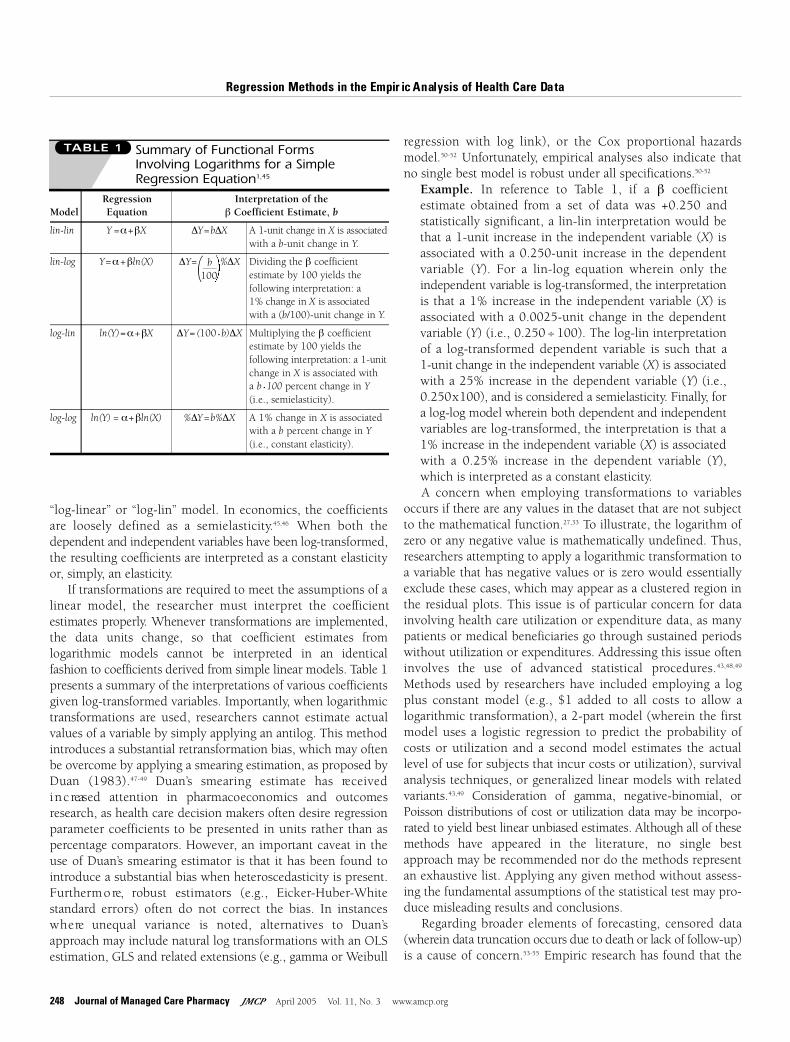
“log-linear” or “log-lin” model. In economics, the coefficientsare loosely defined as a semielasticity.45,46 When both thedependent and independent variables have been log-transformed,the resulting coefficients are interpreted as a constant elasticityor, simply, an elasticity.

If transformations are required to meet the assumptions of alinear model, the researcher must interpret the coefficient estimates pro p e r l y. Whenever transformations are implemented,the data units change, so that coefficient estimates from logarithmic models cannot be interpreted in an identical fashion to coefficients derived from simple linear models. Table 1presents a summary of the interpretations of various coefficientsgiven log-transformed variables. Importantly, when logarithmictransformations are used, researchers cannot estimate actualvalues of a variable by simply applying an antilog. This methodintroduces a substantial retransformation bias, which may oftenbe overcome by applying a smearing estimation, as proposed byDuan (1983).4 7 - 4 9 D u a n ’s smearing estimate has re c e i v e di n c reased attention in pharmacoeconomics and outcomesresearch, as health care decision makers often desire regressionparameter coefficients to be presented in units rather than aspercentage comparators. However, an important caveat in theuse of Duan’s smearing estimator is that it has been found tointroduce a substantial bias when heteroscedasticity is present.F u rt h e rm o re, robust estimators (e.g., Eicker- H u b e r-White standard errors) often do not correct the bias. In instancesw h e re unequal variance is noted, alternatives to Duan’sapproach may include natural log transformations with an OLSestimation, GLS and related extensions (e.g., gamma or Weibull

regression with log link), or the Cox proportional hazardsmodel.50-52 Unfortunately, empirical analyses also indicate thatno single best model is robust under all specifications.50-52

Example. In reference to Table 1, if a β coefficient estimate obtained from a set of data was +0.250 and statistically significant, a lin-lin interpretation would bethat a 1-unit increase in the independent variable (X) isassociated with a 0.250-unit increase in the dependentvariable (Y). For a lin-log equation wherein only the independent variable is log-transformed, the interpre t a t i o nis that a 1% increase in the independent variable (X) isassociated with a 0.0025-unit change in the dependentvariable (Y) (i.e., 0.250 ÷ 100). The log-lin interpretationof a log-transformed dependent variable is such that a 1-unit change in the independent variable (X) is associatedwith a 25% increase in the dependent variable (Y) (i.e.,0.250x100), and is considered a semielasticity. Finally, fora log-log model wherein both dependent and independentvariables are log-transformed, the interpretation is that a1% increase in the independent variable (X) is associatedwith a 0.25% increase in the dependent variable (Y),which is interpreted as a constant elasticity.A concern when employing transformations to variables

occurs if there are any values in the dataset that are not subjectto the mathematical function.27,33 To illustrate, the logarithm ofzero or any negative value is mathematically undefined. Thus,researchers attempting to apply a logarithmic transformation toa variable that has negative values or is zero would essentiallyexclude these cases, which may appear as a clustered region inthe residual plots. This issue is of particular concern for datainvolving health care utilization or expenditure data, as manypatients or medical beneficiaries go through sustained periodswithout utilization or expenditures. Addressing this issue ofteninvolves the use of advanced statistical pro c e d u re s .4 3 , 4 8 , 4 9

Methods used by researchers have included employing a logplus constant model (e.g., $1 added to all costs to allow a logarithmic transformation), a 2-part model (wherein the firstmodel uses a logistic regression to predict the probability ofcosts or utilization and a second model estimates the actuallevel of use for subjects that incur costs or utilization), survivalanalysis techniques, or generalized linear models with relatedv a r i a n t s .4 3 , 4 9 Consideration of gamma, negative-binomial, orPoisson distributions of cost or utilization data may be incorpo-r a t e d to yield best linear unbiased estimates. Although all of thesem e t h o d s have appeared in the literature, no single bestapproach may be recommended nor do the methods representan exhaustive list. Applying any given method without assess-ing the fundamental assumptions of the statistical test may pro-duce misleading results and conclusions.

Regarding broader elements of forecasting, censored data( w h e rein data truncation occurs due to death or lack of follow-up)is a cause of concern.53-55 Empiric research has found that the


Summary of Functional Forms Involving Logarithms for a SimpleRegression Equation1,45

TABLE 1

Regression Interpretation of theModel Equation β Coefficient Estimate, b

lin-lin Y =α+βX ΔY=bΔX A 1-unit change in X is associatedwith a b-unit change in Y.

lin-log Y=α+βln(X) ΔY= %ΔX Dividing the β coefficient estimate by 100 yields the following interpretation: a 1% change in X is associatedwith a (b/100)-unit change in Y.

log-lin ln(Y)=α+βX ΔY=(100 • b)ΔX Multiplying the β coefficient estimate by 100 yields the following interpretation: a 1-unitchange in X is associated witha b • 100 percent change in Y(i.e., semielasticity).

log-log ln(Y) = α+βln(X) %ΔY =b%ΔX A 1% change in X is associated with a b percent change in Y(i.e., constant elasticity).

100( b




censored nature of costs may result in biased estimates if notappropriately controlled.56 Remedial measures that have beensuggested involve applications of survival analysis althoughresearch has demonstrated that these techniques may not necessarily be appropriate and that nonparametric methodsmay be better suited.57

■ ■ Applications in Managed Care

In a purely hypothetical scenario with relevance to managedcare or formulary decision making, an analyst may want to usea managed care dataset to ascertain whether health care cost differences exist between therapeutic options for patients withheart failure. Thus, the dependent variable of interest would betotal health care costs. Furthermore, the analyst may also bei n t e rested in determining the related predictors of hospitalization,defining whether hospitalization occurred as a second dependentvariable that is dichotomous (i.e., hospitalization=1 , no hospital-ization = 0). Given that retrospective analysis of administrativeclaims data lacks randomization and fully experimentalmethodologies, relevant confounding variables must be includedwithin the re g ression model to statistically control for diff e re n c e sbetween study gro u p s .1 1 Thus, in this example, simply comparingunadjusted total health care costs (or whether a patient was orwas not hospitalized) between the therapeutic options withoutc o n t rolling for confounders is inappropriate; re g ression analysesare required.

Contingent upon a thorough literature review of predictorsof cost and/or hospitalization in heart failure patients, the specification of a regression model in this hypothetical caseshould provide a theoretical basis for the variables that areultimately included in the analysis. In pharmacoeconomic oroutcomes research, these independent variables may includerisk adjustment measures to control for case mix severity (e.g., Chronic Disease Score [CDS] based upon prescriptiondrug use, Charlson Index based upon International Classificationof Diseases, 9th Revision, Clinical Modification codes), patient characteristics (e.g., age, sex), comorbid conditions, pre t re a t m e n tcosts, and treatment gro u p s .5 8 - 6 0 A d d i t i o n a l l y, medication adhere n c e(e.g., Medication Possession Ratio) and insurance or providercharacteristics (e.g., type of health care organization, Medicare,Medicaid, prescriber specialty) may be deemed i m p o rtant toconsider within a re s e a rch question.6 1 I n c o r p o r a t i n g some of theseconsiderations, a theoretical model may be proposed in comparingt reatment options (Treatment O n e, Treatment Tw o, and Treatment T h re e) as

Expenditures = f(Risk, Patient, Comorbidities, PretreatmentCost, Treatment Group),

which appears in regression form as

Ex p e n d i t u res = α + β1C D S + β2Age + β3S ex + β4C o m o r b i d i t y +β5 Treatment One +β6Treatment Two + ε

w h e re Sex, Comorbidity, Tre a t m e n t O n e, and Tre a t m e n t Tw o a re definedas dichotomous dummy variables (variables with only 2 values:0 or 1). Treatment Three is considered the baseline used for comparison. Given that the total number of dummy variablesre q u i red is equal to 1 less than the total number of categories to be compared, a single dummy variable is used forSex, while 2 dummy variables are used for the treatment groups.Comorbidities may also be coded as dummy variables, with thepresence of the condition coded as 1 and absence coded as 0.Examples relevant to heart failure may include a past history ofmyocardial infarction or stroke and can extend to include the presence of diabetes, atrial fibrillation, renal disease, orhypertension.

Concerning the second dependent variable in the example(i.e., hospitalization), when binary categorical variables are usedas a dependent variable, a logistic regression may be considered;this may also be extended to ascertain predictors of treatmentsuccess (i.e., treatment success=1, treatment failure=0).62

Example 1. Armstrong and Malone (2002) conducted anassessment of asthma-related costs associated with fluticasone versus leukotriene modifier use, in which thedependent variable was log-transformed post-asthmacost and independent variables included age, sex, l o g - t r a n s f o rmed pre-asthma cost, CDS, presence ofchronic obstructive pulmonary disease, treatment group(i.e., fluticasone or leukotriene modifier), and the use ofc e rtain medications prior to the study period (i.e., numberof short-acting β-agonist canisters used and dummycodes representing the use of long-acting β-agonists,theophylline or mast cell stabilizers, or oral corticos-teroids).63

Example 2. McLaughlin, Eaddy, and Grudzinski (2004)analyzed depre s s i o n - related charges associated with t reatment with sertraline and citalopram.6 4 The dependentvariable, treatment charges, was transformed via naturallogarithm specifically due to the detection of heteroscedasticity. The independent variables includedage, sex, geographic region, natural log of treatmentc h a rges prior to the study period, the presence of comorbidites (either mental or nonmental health), thetype of managed care institution, the physician specialty,the use of emergency department or hospital servicesprior to the study period, and the year of initial diagnosis.

■ ■ ConclusionR e g ression is a powerful and commonly used statistical technique that gives researchers the ability to quantify mathe-matical relationships for purposes of description, hypothesistesting, or p rediction. Before a proper analysis can begin, anu n d e r s t a n d i n g is necessary of correlation, of the assumptions of a classical linear regression model, and of the importance ofresidual assessments. Despite its complexities, the flexibility



of regression makes it especially applicable in certain settings,enabling decision makers to analyze complex phenomena andanswer questions that other statistical methods inadequatelyaddress. Contingent upon the specific research question, anumber of extensions to basic regression techniques may beexplored so that this method can be used appropriately in p h a rmacoeconomic or outcomes re s e a rch and assist in form u l arydecision making. The increased availability of administrativedatabases containing medical and pharmacy claims data mayprovide those in managed care settings with a greater ability toevaluate treatments and practice patterns. Given that administra-tive data are observational rather than experimental, it is criticalthat analysts and decision makers be versed in appropriate statistical methods to design investigations or evaluate empiricfindings.

DISCLOSURES

No outside funding supported this study. The author discloses no potentialbias or conflict of interest relating to this article.

REFERENCES

1. Studenmund AH. Using Econometrics: A Practical Guide. 4th ed. Boston:Addison Wesley; 2001.

2. Armstrong EP, Manuchehri F. Ambulatory care databases for managed careorganizations. Am J Health Syst Pharm. 1997;54:1973-83.

3. Johnson N. The six-step process for conducting outcomes analyses usingadministrative databases. Formulary. 2002;37:362-64.

4. Gandi SK, Salmon JW, Kong SX, Zhao SZ. Administrative databases andoutcomes assessment: an overview of issues and potential utilities. J ManagCare Pharm. 1999;5(3):215-22.

5. Else BA, Armstrong EP, Cox ER. Data sources for pharmacoeconomic andhealth services research. Am J Health Syst Pharm. 1997;54:2601-08.

6. Neter J, Kutner MH, Nachtscheim CJ, Wasserman W. Applied LinearStatistical Models. 4th ed. Chicago: Irwin, McGraw-Hill; 1996.

7. Shott S. Statistics for Health Professionals. Philadelphia: W.B. Saunders; 1990.

8. Dawson B, Trapp RG. Basic and Clinical Biostatistics. 3rd ed. New York:Lange Medical Books, McGraw-Hill; 2001.

9. Glantz SA, Slinker BK. Primer of Applied Regression and Analysis of Variance.New York: McGraw-Hill; 1990.

10. Cook TD, Campbell DT. Quasi-experimentation: Design and Analysis Issuesfor Field Settings. Boston: Houghton Mifflin; 1979.

11. Motheral BR, Fairman KA. The use of claims databases for outcomesresearch: rationale, challenges, and strategies. Clin Ther. 1997;19:346-66.

12. Motheral BR. Research methodology: hypotheses, measurement, reliability,and validity. J Manag Care Pharm. 1998;4(4):382-88.

13. Richards KM, Shepherd MD. Subject review: claims data and drawingappropriate conclusions. J Manag Care Pharm. 2002;8(2):152.

14. Motulsky H. Intuitive Biostatistics. New York: Oxford University Press; 1995.

15. Gujarati DN. Basic Econometrics. 3rd ed. New York: McGraw-Hill; 1995.

16. Johnston J. Econometric Methods. 3rd ed. New York: McGraw-Hill; 1984.

17. Greene WH. Econometric Analysis. 4th ed. Upper Saddle River, NJ:Prentice-Hall; 2000.

18. O’Brien BJ, Drummond MF. Statistical versus quantitative significance in thesocioeconomic evaluations of medicines. P h a rmacoeconomics. 1 9 9 4 ; 5 : 3 8 9 - 9 8 .

19. Drummond M, O’Brien B. Clinical importance, statistical significance, andthe assessment of economic and quality-of-life outcomes. Health Econ. 1 9 9 3 ; 2 :205-12.

20. Stevens J. Applied Multivariate Statistics for the Social Sciences. 3rd ed.Mahwah, NJ: Lawrence Erlbaum Associates; 1996.

21. Park C, Dudycha A. A cross validation approach to sample size determ i n a t i o nfor regression models. J Am Stat Assoc. 1974;69:214-18.

22. Cohen J. Statistical power analysis for the behavioral sciences. 2nd ed.Hillsdale, NJ: Lawrence-Erlbaum Associates; 1988.

23. Hardy MA. Regression with Dummy Variables. Newbury Park, CA: SagePublications; 1993.

24. Frisch R. Statistical Conference Analysis by Means of Complete RegressionsSystems. Publication Number 5. Oslo: University of Oslo, Institute ofEconomics; 1934.

25. Montgomery D, Peck E. Introduction to Linear Regression Analysis. NewYork: John Wiley & Sons; 1982.

26. Achen CH. Interpreting and Using Regression. Beverly Hills, CA: SagePublications; 1982.

27. Carrol RJ, Rippert D. Transformation and Weighting in Regression. New York:Chapman and Hall; 1988.

28. Durbin J, Watson GS. Testing for serial correlation in least-squares re g re s s i o n .Biometrika. 1951;38:159-71.

29. Geary RC. Relative efficiency of a count of sign changes for assessing re s i d u a la u t o re g ression in least squares re g ression. B i o m e t r i k a . 1970;57:123-27.

30. Breusch TS. Testing for autocorrelation in dynamic linear models.Australian Econ Pap. 1978;17:334-55.

31. Godfrey LG. Testing against general autoregressive and moving averageerror models when the regressors include lagged dependent variables.Econometrica. 1978;46:1293-1302.

32. Hamilton JD. Time Series Analysis. Princeton: Princeton University Press; 1994.

33. Park RE. Estimation with heteroscedastic error terms. Econometrica. 1966;34:888.

34. Glejser H. A new test for hetero s c e d a s t i c i t y. J Am Stat Assoc. 1 9 6 9 ; 6 4 : 3 1 6 - 2 3 .

35. Breusch TS, Pagan AR. A simple test for heteroscedasticity and randomcoefficient variation. Econometrica. 1979;47:1287-94.

36. Goldfeld SM, Quandt RE. Nonlinear Methods in Econometrics. Amsterdam:North-Holland Publishing Company; 1972.

37. White H. A heteroscedasticity consistent covariance matrix estimator anda direct test of heteroscedasticity. Econometrica. 1980;48:817-18.

38. Eicker F. Limit theorems for regressions with unequal and dependenterrors. Proceedings of the Fifth Berkeley Symposium on Mathematical Statistics andProbability. Berkeley: University of California Press; 1967:59-82.

39. Huber PJ. The behavior of maximum likelihood estimates under nonstan-dard conditions. Proceedings of the Fifth Berkeley Symposium on MathematicalStatistics and Probability. Berkeley: University of California Press; 1967:221-33.

40. White H. A heteroscedasticity-constant covariance matrix estimator and adirect test for heteroscedasticity. Econometrica. 1980;48:827-38.

41. Bera A, Higgins M. ARCH models; properties, estimation, and testing. J Econ Surveys. 1993;7:305-66.

42. Fox J. Regression Diagnostics. Newbury Park, CA: Sage Publications; 1991.

43. Diehr P, Yanez D, Ash A, Hornbrook M, Yin DY. Methods for analyzinghealth care utilization and costs. Annu Rev Public Health. 1999;20:125-44.

44. Zhou X, Melfi CA, Hui SL. Methods for comparison of cost data. AnnIntern Med. 1997;127:752-56.

45. Wooldridge JM. Introductory Econometrics: A Modern Approach. 2nd ed.Stamford, CT: South-Western, Thomson; 2003.

46. Barnett RA, Ziegler MR. Applied Calculus for Business, Economics, LifeSciences, and Social Sciences. 5th ed. New York: MacMillan; 1994.




47. Duan N. Smearing estimate: a nonparametric retransformational method. J Am Stat Assoc. 1983;78:605-10.

48. Manning WG. The logged dependent variable, heteroscedasticity, and theretransformation problem. J Health Econ. 1998;17:283-95.

49. Mullahy J. Much ado about two: reconsidering retransformation and thetwo-part model in health econometrics. J Health Econ. 1998;17:247-81.

50. Manning WG, Mullahy J. Estimating log models: to transform or not totransform. J Health Econ. 2001;20:461-94.

51. Basu A, Manning WG, Mullahy J. Comparing alternative models: log versus Cox proportional hazard? Health Econ. 2004;13:749-65.

52. Berry WD, Feldman S. Multiple Regression in Practice. Newbury Park, CA:Sage Publications; 1985.

53. Bang H, Tsiatis AA. Estimating medical costs with censored data.Biometrika. 2000;87:329-43.

54. Lin DY. Linear regression analysis of censored medical costs. Biostatistics.2000;56:775-78.

55. Zhao H, Tian L. On estimating medical cost and incremental cost-effectiveness ratios with censored data. Biometrics. 2001;57:1002-08.

56. Fenn P, McGuire A, Phillips V, Backhouse M, Jones D. The analysis of cen-sored treatment cost data in economic evaluation. Med Care. 1995;33:851-63.

57. Etzioni RD, Feuer EJ, Sullivan SD, Lin D, Hu C, Ramsey S. On the use ofsurvival analysis techniques to estimate medical care costs. J Health Econ.1999;18:365-80.

58. Von Korff M, Wagner EH, Saunders K. A chronic disease score from automated pharmacy data. J Clin Epidemiol. 1992;45:197-203.

59. Clark DO, Von Korff M, Saunders K, Baluch WM, Simon GE. A chronicdisease score with empirically derived weights. Med Care. 1995;33:783-95.

60. Charlson ME, Pompei P, Ales KL, McKenzie CR. A new method of classifyingp rognostic comorbidity in longitudinal studies: development and validation.J Chronic Dis. 1987;40:373-83.

61. Sclar DA, Chin A, Skaer TL, et al. Effect of health education in promotingprescription refill compliance among patients with hypertension. Clin Ther.1991;13:489-95.

62. Abarca J, Armstrong EP. Multiple logistic regression: a statistical method to evaluate predictors of hospitalizations. Formulary. 2000;35:832-41.

63. Armstrong EP, Malone DC. Fluticasone is associated with lower asthma-related costs than leukotriene modifiers in a real-world analysis.Pharmacotherapy. 2002;22:1117-23.

64. McLaughlin TP, Eaddy MT, Grudzinski AN. A claims analysis comparingcitalopram with sertraline as initial pharmacotherapy for a new episode ofd e p ression: impact on depre s s i o n - related treatment costs. Clin Ther. 2 0 0 4 ; 2 6 : 1 1 5 - 2 4 .



R e gression Methods in the Empiric Analysis of Health ... e gression Methods in the Empiric...

Documents

Transcript of R e gression Methods in the Empiric Analysis of Health ... e gression Methods in the Empiric...