R & D, Patents, and Productivity
35
This PDF is a selection from an out-of-print volume from the National Bureau of Economic Research Volume Title: R & D, Patents, and Productivity Volume Author/Editor: Zvi Griliches, ed. Volume Publisher: University of Chicago Press Volume ISBN: 0-226-30884-7 Volume URL: http://www.nber.org/books/gril84-1 Publication Date: 1984 Chapter Title: Tests of a Schumpeterian Model of R&D and Market Structure Chapter Author: Richard Levin, Peter C. Reiss Chapter URL: http://www.nber.org/chapters/c10049 Chapter pages in book: (p. 175 - 208)
Transcript of R & D, Patents, and Productivity

This PDF is a selection from an out-of-print volume from the National Bureauof Economic Research
Volume Title: R & D, Patents, and Productivity
Volume Author/Editor: Zvi Griliches, ed.
Volume Publisher: University of Chicago Press
Volume ISBN: 0-226-30884-7
Volume URL: http://www.nber.org/books/gril84-1
Publication Date: 1984
Chapter Title: Tests of a Schumpeterian Model of R&D and Market Structure
Chapter Author: Richard Levin, Peter C. Reiss
Chapter URL: http://www.nber.org/chapters/c10049
Chapter pages in book: (p. 175 - 208)

8 Tests of aSchumpeterian Model ofR&D and Market StructureRichard C. Levin and Peter C. Reiss
8.1 Introduction
Schumpeter's (1950) ideas about the role of innovation in moderncapitalist economies have inspired a substantial literature on the relationship between market structure and innovative activity. This literaturehas focused on Schumpeter's observation that seller concentration influences the appropriability of R&D. Unfortunately, as is apparent inthe surveys of Kamien and Schwartz (1975) and Scherer (1980), it isunclear whether highly concentrated markets enhance the appropriability of the returns to R&D (e.g., Schumpeter 1950) or whether theopposite is true (Fellner 1951; Arrow 1962). In either case, industryconcentration is viewed as an important determinant of R&D intensity.
With few exceptions (notably Phillips 1966, 1971), it was not untilrecently that economists turned their attention to the reciprocal influenceof R&D on market structure. This new literature has emphasizedSchumpeter's oft-cited notion of "creative destruction," where marketstructure is influenced by past and current innovative successes andfailures. Specifically, innovation generates transient market power; this,in turn, is eroded by rival innovation and imitation. Thus, a truly Schumpeterian framework requires that both market structure and R&D betaken as endogenous variables. Seen in this perspective, the relation ofR&D and market structure must be explained by an appeal to morefundamental factors that jointly determine concentration and R&D: the
Richard C. Levin is a professor in the Department of Economics and the School ofManagement, Yale University. Peter C. Reiss is an assistant professor in the StanfordUniversity Graduate School of Business.
The authors gratefully acknowledge the support of the Division of Policy Research andAnalysis of the National Science Foundation under grant PRA-8019779.
175

176 Richard C. Levin /Peter C. Reiss
structure of demand; the richness of technological opportunities; and thetechnological and institutional conditions governing appropriability.
A number of recent theoretical papers have attempted to capture theessence of this Schumpeterian simultaneity. Among these contributionsare Dasgupta and Stiglitz (1980a, 1980b), Futia (1980), Lee and Wilde(1980), Levin (1978), Loury (1979), and Nelson and Winter (1977,1978,1980).1 The approach taken by Nelson and Winter is the most comprehensive in its representation of the relevant forces influencing marketstructure and R&D intensity. The price of this generality is high, sincetheir models are analytically intractable and are open only to simulation.By contrast, many of the remaining models are stark and highly stylized;each omits aspects of technology and competition that are important for abroader understanding of the relationship between market structure andR&D. For example, none of the above models is truly dynamic; marketstructure is represented by the number of identical firms; only Futiaexplicitly recognizes R&D spillovers where firms benefit from the effortsof rivals; and finally, no attention is paid to other activities, such asadvertising, that affect market structure.
The problems hampering theoretical treatments of the simultaneityissue have made rigorous tests of the Schumpeterian process extremelydifficult. To date only Levin (1981) and Farber (1981) have explored thesimultaneity issue in any detail. Only Levin has attempted to test for thepresence of simultaneity among the relevant variables, but Levin's model(in which concentration, private and government, R&D, advertising,and price-cost margins are determined simultaneously) is specified in theloose, eclectic manner that is characteristic of most empirical work inindustrial organization. Although the findings are encouraging, they canonly be regarded as a preliminary test of the neo-Schumpeterian theories.
In this paper we provide a more exacting empirical test. Unfortunately,in our efforts to formulate precise hypotheses, we are forced to ignoreseveral aspects of Schumpeterian dynamics. Nonetheless, we are able toincorporate several important features of reality which have heretoforebeen missing in formal models of the R&D process. We begin with whatis perhaps the simplest of the theoretical models of R&D and marketstructure, the Dasgupta-Stiglitz (1980a) model of noncooperative oligopoly with free entry. We generalize this model by adding two significant features. First, we allow for spillovers in the knowledge generated byR&D. Hence, some fraction of the returns to each firm's R&D effortsare appropriated by its rivals. Although we are not able at this stage to
1. Although they do not discuss the simultaneous determination of R&D activity andmarket structure, the work of Pakes and Schankerman (this volume) on the determinants ofR&D spending is akin to the papers cited here in clear identification of demand, technological opportunity, and appropriability as central exogenous variables.
177 Tests of a Schurnpeterian Model of R&D and Market Structure
incorporate a specific allocation of investment to imitative effort, asNelson and Winter do, we believe that our characterization of R&Dspillovers illuminates important aspects of the appropriability problem,as we explain below. Second, we include advertising expenditures amongthe decision variables of the firm. Like R&D, advertising is an instrument of competition, and in many industries it is of greater empiricalconsequence than R&D. By thus enriching the model, we hope to gain amore precise understanding of the role of both R&D and advertising inSchumpeterian competition.
An attractive feature of our approach is that the general model contains a family of nested models that can be tested using classical procedures. For example, by constraining the value of certain parameters(namely, the degree of R&D spillovers and the elasticity of demand withrespect to advertising) the Dasgupta-Stiglitz model falls out as a specialcase of our own model. In addition, questions concerning the effects ofimperfect appropriability of R&D returns can be reduced to considerations of the magnitudes or signs of certain parameters in the model.
We believe our approach to be an attractive one, but we must cautionthe reader at the outset that limitations of both theory and data stillpreclude a fully satisfactory treatment of the issues we explore here. Themodel remains quite stark, abstracting from at least four issues of undoubted importance. First, the model is one of a static industry equilibrium, which is hardly in the spirit of the Schumpeterian dynamic disequilibrium arguments. Second, we take no account of uncertainty,which even in the absence of risk aversion has important implications forthe allocation of R&D effort. Third, to make the analysis tractable, weconsider only symmetric industry equilibria, where all firms within anindustry are identical. Fourth, we consider only cost-reducing R&D,neglecting the well-known fact that most industries devote a major shareof their innovative efforts to developing new products and improving thequality of existing products. In future work, we plan to generalize ourmodel to take account of dynamics, uncertainty, asymmetry, and productR&D.
Limitations of the data constrain our efforts as well. Our model isdesigned for testing on a cross section of industries, but R&D data areavailable for industries only at a highly aggregated level, requiring us toaggregate data on other variables up to this level. Even more serious aredeficiencies in the operational measures of technological opportunity andappropriability. In this paper, we rely on relatively crude proxies.However, together with several colleagues, we have recently initiatedwork on the direct measurement of opportunity and appropriabilityconditions through a survey of R&D managers. When collected, thesedata should substantially improve the reliability of the empirical resultsobtainable with this or any related econometric model.

178 Richard C. Levin/Peter C. Reiss
The remainder of the paper is organized as follows. Section 8.2 presents and analyzes the model. Section 8.3 develops the empirical specification. The data and the econometric techniques are discussed insection 8.4. In section 8.5 the econometric results are presented andinterpreted, and section 8.6 indicates directions for future research.
8.2 A Model of R&D with Spillovers
We begin by considering a firm that seeks to maximize profit with theuse of three instruments: output, R&D expenditures, and advertisingexpenditures. Following Dasgupta and Stiglitz, we assume that a firm'sR&D expenditure serves to shift downward its unit cost function, whichis independent of output, but we generalize their formulation to includethe effect of industrywide R&D on cost. Thus, unit cost of firm i is
(1)
where Xi is the R&D expenditure of the ith firm, and Z is the sum of theR&D expenditures of all firms in the industry, including firm i. 2 It isfurther assumed that CI, C2 < 0, and CII, C22 > 0; that is, there are positivebut decreasing returns to both own R&D and to industrywide R&D.
This formulation emphasizes an important aspect of R&D technologyneglected in most analytic models-external economies. An increase inthe R&D expenditures of firm i not only reduces its own cost, but it also,through its "spillover" effect on Z, reduces the cost of all other firms inthe industry. This characterization captures a central aspect of theappropriability issue; specifically, the cost function indicates the technological dimension of appropriability. To the extent that unit costreduction is very elastic with respect to increments in the industrywidepool of R&D (holding own R&D constant), we infer that costlessimitation is relatively easy, or that, technologically, the returns to R&Dare relatively inappropriable. We shall indicate shortly how appropriability also has structural and behavioral dimensions.
Since our primary interest attaches to the analysis of R&D, we take asomewhat simpler approach with respect to advertising and its effect ondemand. In particular, we assume that advertising shifts the industrydemand curve. In principle, we could model advertising as altering thefirm's own demand curve as well as spilling over to alter the demandsfacing all other firms. Such a characterization would reveal clearly thecomplete analogy between the roles of appropriability and R&D, sincethe appropriability of advertising also has technological, structural, andbehavioral dimensions. Instead, we simply represent the industry inversedemand curve as:
2. Equation (1) can be generalized to include spillovers of R "& D undertaken in otherindustries.
179 Tests of a Schumpeterian Model of R&D and Market Structure
(2) p = p(Q,A),
where Q = ~qi represents industry output, and A = ~ai represents totaladvertising expenditures of all firms in the industry. We further assumethat PI < 0, P2> 0, and P22 < O.
The problem facing the ith firm is, therefore,
(3)
We assume that firms entertain Cournot conjectures regarding the outputand advertising levels of all other firms. That is, we assume that the ithfirm conjectures that dQldqi = 1 and dAldai = 1. However, to bringclearly to the fore the full range of issues regarding the appropriability ofR&D, we parameterize the conjectural variation with respect toR&D. That is, we let dZIdxi = ai. Later, we shall explore several specialcases by fixing ai.
We now write down the first-order conditions for the maximization ofthe ith firm's profit:
(4)
(5)
(6)
P(l-~)=C,
- (CI + C28Jqi = 1, and
where E = pi QPI, the price elasticity of demand,3 and Si = qil Q, themarket share of the ith firm.
We assume free entry such that the maximized profits of all firms in theindustry are greater than or equal to zero, while profits of all firms outside(potential entrants) are less than or equal to zero for all nonnegativelevels of output. We further restrict our attention to symmetric equilibria,where all firms in the industry behave identically. This latter restriction is,of course, less than desirable in a model purporting to represent Schumpeterian competition, but we have found that consideration of asymmetric equilibria raises some extremely difficult analytical problems.
Dasgupta and Stiglitz have shown that, given certain restrictions on theparameters, symmetric free entry equilibria exist. Somewhat more complicated restrictions on the parameters are necessary in the presentmodel, but a wide range of parameter values remain consistent withequilibrium. Dasgupta and Stiglitz have also derived conditions underwhich the profit of each firm in the industry is approximately equal to zeroin a symmetric equilibrium. Of course, it is perfectly plausible that the
3. Dasgupta and Stiglitz (1980a) use the notation E to represent the quantity elasticity ofinverse demand. We find that intuition is facilitated by reverting to the more customarynotation.
180 Richard C. Levin/Peter C. Reiss
technology of R&D (or of advertising) would be such that equilibriumcontains a very small number of firms earning nonnegligible profit, butthe entry of one additional firm would result in negative profits for all. 4 Inwhat follows, we assume that the zero-profit condition can be invoked.Thus, we close the model by noting that each firm earns zero profit inequilibrum:
(7)
Before proceeding, it is worth pointing out (in the manner of Dasguptaand Stiglitz) that conditions (4)-(7) may be used to illustrate that amarket equilibrium involving cost-reducing and demand-shifting activities, such as R&D and advertising, will not result in a socially optimalallocation of resources. Conditions (4) and (7) indicate that prices mustdeviate from marginal cost to sustain R&D and advertising expenditures. Moreover, the left-hand sides of (5) and (6) show that the marginalprivate benefit of R&D and advertising depends on the firm's scale ofoutput, whereas social optimality would require that the market output,Q, be substituted for qi in these expressions.
We now proceed to analyze the market equilibrium in greater detail.First, note that in a symmetric equilibrium with n identical firms, qi == q,Xi == X, ai == a, 0i == e, and Si == 1/n, for all firms. The zero-profit conditioncan then be summed over all firms by multiplying both sides of (7) by n toyield:
(8) [p(Q, A) - c(x, Z)] Q == nx + na.
Dividing both sides by pQ, we havep -c
(9) p = R+S,
where the left-hand side is the Lerner index of monopoly power, R, is theratio of industry R&D to sales, and 5 is the ratio of advertising to sales.Combining (9) and (4), we have
(10)1- == E (R + 5),n
where 1/n is the Herfindahl index of concentration. This striking resultsays that industry concentration is proportionate to the sum of R&D andadvertising intensity, where the elasticity of demand is the factor ofproportionality. Our result parallels that of Dasgupta and Stiglitz, who,by neglecting advertising (5 == 0), arrive at 1/n == ER.
We choose to treat (10) as a structural equation for concentration in theeconometric work which follows. Since we derived (10) from the first-
4. The problem with the zero-profit condition arises from the requirement that n beinteger valued.

181 Tests of a Schumpeterian Model of R&D and Market Structure
order condition (4) and the zero-profit condition (7), we now use (5) and(6) to derive structural equations for R&D intensity and advertisingintensity, respectively.
Multiplying both sides of (5) by R = xlpq gives:
(11)
(13)
Simple manipulation of (11) yields
(12) - (cIx + czze)E- = R.c cn p
But inspection of equation (9) reminds us that clp = 1 - (R + S). We alsoobserve that - (cIxl c) can be interpreted as the elasticity of unit cost withrespect to x, holding Z constant, which we will denote as a = a(xIZ), andthat - (czZlc) is the elasticity of unit cost with respect to Z, holding xconstant, which we denote as "I = 'Y(Zlx). It follows that (12) can berewritten as:
R = a + "Ie .1 - (R + S) n
The numerator of the left-hand side of (13) is the ratio of R&D tosales, while the denominator is the share of sales revenue that is devotedto neither R&D nor advertising. In zero-profit equilibrium this is justequivalent to the ratio of production cost to revenue. Thus, the left-handside of (13) is simply the ratio of R&D to total production cost, a variantof the more familiar representation of R&D intensity, typically used ineconometric work.
We can interpret (13) as a structural equation in which R&D intensitydepends on two terms. The first, a, is the elasticity of unit cost withrespect to own R&D, holding industrywide R&D constant. It seemsreasonable to interpret a as a measure of technological opportunity,indicating the responsiveness of cost to own research effort. The secondterm, "lain, has three components, each of which represents one of thedimensions of appropriability mentioned previously. We noted that "I,the elasticity of unit cost with respect to industrywide R&D (holdingown R&D constant), is a reasonable measure of the technologicaldimension of appropriability, since it represents the extent to which afirm benefits from an increase in the common pool of R&D effort. Onthe other hand, since a firm's own R&D effort augments the commonpool, higher levels of "I are associated with greater R&D intensity aslong as the conjectural variation, 8, is positive.
Appropriability has a structural dimension as well, which was emphasized by Schumpeter (1950) and later by Galbraith (1956). For any giventechnology of R&D and market size, a firm's appropriable benefits from

182 Richard C. Levin IPeter C. Reiss
augmenting the common pool of knowledge depend on its market share,which is lin in a symmetric equilibrium. On the conjecture that rivals donot respond (8 == 1), a 1 percent increase in own R&D produces a linpercent increase in industrywide R&D. Thus, whereas a monopolist'scosts fall by "{ percent for a 1 percent increase in its contribution to thecommon pool, an oligopolist's costs fall only by "{In percent. Through thismechanism, the intensity of R&D increases with the greater appropriability associated with a more concentrated market structure.
Finally, there is a behavioral dimension to appropriability, representedhere by the conjectural variation parameter, 8. It is easy to show that theCournot conjecture, 8 == 1, results in a Nash equilibrium when combinedwith our previous assumptions that firms have Cournot conjectures inoutput and advertising decisions. But some informal arguments concerning the disincentive effects of spillover in R&D implicity contain presumptions that 8 < 1. To the extent that firm j can costlessly borrowknowledge from firm i's R&D effort, it may choose to be a free rider andcut back on its own R&D. If the free-rider effect is sufficiently strong, emay even be negative; that is, a one dollar increase in R&D expenditureby firm i may produce cutbacks in the R&D expenditures of the remaining firms that exceed one dollar in the aggregate. Such negative conjectural variations produce market equilibria that are not Nash equilibria,but the idea that free-rider effects are important in R&D is sufficientlywell entrenched in the literature (e.g., Nelson 1959) to warrant testing forevidence of its presence.
In the empirical work that follows, we will examine several specialcases of the model in which etakes on prespecified values, as well as thecase in which 8 is free to vary. In particular, we will examine cases inwhich the value of 8 is assumed to be 0,1, and n, respectively. In the firstcase, the free-rider effect is such that rivals exactly offset a change in firmi's R&D, leaving industry R&D constant. The second is the CournotNash case. In the third case, each firm behaves as if it expects its action tobe matched by all others. This is the R&D analog of the Chamberlinian"constant market shares" conjecture. We shall test whether the datapermit rejection of any of these three hypotheses about the value of e.
Equations (10) and (13) represent structural equations for concentration and R&D intensity, respectively. We now derive a third equationfor advertising intensity. Multiplying both sides of the first-order condition (6) by Alp and dividing both sides by qi gives:
A A(14) P2 - == - .
P pqi
The left-hand side of (14) is the advertising elasticity of inverse demand,which we denote as 1")- Dividing both sides of (14) by n we have
183
(15)
Tests of a Schumpeterian Model of R&D and Market Structure
~==Sn '
(17)
where S is the ratio of industry advertising to sales, AIpQ.It is easily shown that this expression for advertising intensity is simply
a generalization of the Dorfman-Steiner (1954) rule to the oligopoly case.Note that at any given price
(16) 11 = ap A = ~ ap QaQ A = 1,aA p aQ p aA Q E
where <P is the advertising elasticity of demand, and E is the price elasticityof demand or, equivalently, the reciprocal of the inverse elasticity ofdemand. Thus, substituting (16) into (15), we have
S==~,En
which is, of course, identical to the familiar Dorfman-Steiner resultwhen, in the monopoly case, n == 1.
To summarize, we have now derived three structural equations representing the simultaneous determination of industry structure, R&D,and advertising intensity:
(10)
(13)
(17)
1n== E(R + S),
R == a + 'Y<P and1 - (R + S) n '
S==±.En
These structural relations are reasonably general, although they do depend on the special assumptions of symmetry and of Cournot conjecturesin advertising and output. 5 In addition, E, <p, a, and 'Y need not be constantparameters. However, by specializing the cost and demand functionsthey become so, and it becomes possible both to solve for reduced formequations for n, R, and S and to operationalize the model for empiricalwork. Thus, we assume that both cost and inverse demand functions haveconstant elasticities, so that
(18) C(x, Z) == ~x-az--y, and
5. It is easy to see that the Dasgupta-Stiglitz model is a special case of our ownimplicitly they asume 'Y = e = O. Under these conditions, the model reduces to twostructural equations for market structure and R&D: lin = ER and RI(l - R) = a. It isreadily verified that these equations are equivalent to those contained in Dasgupta-Stiglitz(1980a).

184 Richard C. Levin/Peter C. Reiss
(19) p(Q, A) = (J"l/EA'llQ-l/E.
The inverse demand function (19), of course, corresponds to the demandfunction:
(20)
8.3 Empirical Specification
The model we have developed consists of three endogenous variables:the Herfindahl index of concentration (H = 1/n), research intensity, andadvertising intensity. These three variables are jointly determined by theparameters of the cost and demand functions, which presumably differacross industries, and by the behavioral parameter, e. We propose to testthe model using cross-section data at the industry level to determinewhether interindustry differences in opportunity, appropriability, anddemand satisfactorily explain differences in concentration, R&D, andadvertising. For the present we assume that e is constant across allindustries, except in the special case where e = n, and we test varioushypotheses concerning its value.
Although the endogenous variables H, R, and S are directly observable(at least in principle), the exogenous parameters E, <p, u, and ~ are not.Since estimates of the price elasticity of demand exist for a wide range ofindustries, we treat Ek as an observable exogenous variable for the kthindustry. Next, to make the estimation problem tractable, we assume thatUk, the elasticity of unit cost with respect to own R&D in the kthindustry, is a function of a vector of observables representing technological opportunity. Similarly, ~k, the elasticity of unit cost with respect toindustrywide R&D, is assumed to be a function of observables representing the degree of R&D spillovers (the technological dimension ofappropriability). Finally, <Pk' the advertising elasticity of demand, isassumed to be a function of observable attributes of the industry's product. In the absence of any strong theoretical presumption, Ctk(·)' ~k(·)'
and <Pk(·) are each assumed to be linear in parameters with an additiveerror term of mean zero. These errors are assumed to be uncorrelatedwith each other and uncorrelated with the error terms in the model'sstructural equations.
We can now write down a system of equations that can be estimated.Assuming that (10) is observed with multiplicative error and takinglogarithms, we have
(21) log H = ao + al(logE) + a2[log(R + S)] + el.
The model makes very precise predictions about the signs and magnitudes of the coefficients of (21). Specifically, we will test the hypotheses,

185 Tests of a Schumpeterian Model of R&D and Market Structure
separately and jointly, that ao = 0 and al = a2 = 1. It should be recalledthat the Dasgupta-Stiglitz model is a special case of our own when <p = "Y= o. We can compare estimates of (21) with estimates of
(22) log H = a~ + at (loge) + a2 (logR) + et,
(24)
to determine whether anything is gained by adding advertising to themodel.
The second equation takes the general form:
(23) R = a(o) + eHy(o) + e2,1- (R + S)
where errors are contained in the a (e) and "Y (e) expressions as notedabove. Substituting for aCe) and "Y(e), we have
R =[bo +( I bmOPPm) +u]1-(R+S) m=l
+ eH[co + C;l CnAPPn) + v] + e2,
where OPPm is an element in an M-dimensional vector of variablesmeasuring technological opportunity, and APPn is an element in anN-dimensional vector of variables measuring the technological conditions of appropriability. Before specifying these opportunity and appropriability measures, two general comments about (24) are in order.
First, the combined error term in equation (24), e2 + u + vaH, hasundesirable properties, except in cases where a is assumed to be eitherzero or n. In the general case, (24) implies that the concentration term,H, has a random coefficient equal to a(eo + v). We will discuss thisproblem in section 8.4.
Second, it will not be possible to identify afrom the parameters of (24),since amultiplies each coefficient in "Y(e). Nevertheless, it will be possibleto test specific hypotheses about the value of a. For example, the hypothesis that a = 0 implies that the coefficients of the last N + 1 terms of theestimated equation are jointly equal to zero. In fact, we cannot distinguish between the hypotheses that a = 0 and "Y = 0, since the lattercarries the same implication for the coefficients of (24). Rejection of thishypothesis, however, is equivalent to rejection of the Dasgupta-Stiglitzspecification, in which "Y = O.
We will also be able to test whether a = n, the "constant R&Dshares" conjecture, since aH = 1 under this assumption. The specification resulting from this hypothesis is not nested in the empirical specification of the general model, since the elements in the APP vector now enterdirectly rather than interactively with H. We can, however, test the

186 Richard C. Levin/Peter C. Reiss
hypothesis e == n against e == O. Unfortunately, the hypothesis thatcon jectures are Cournot (e == 1) cannot be tested.
Given the available data, we have at best crude proxies for technological opportunity and appropriability. As noted in section 8.1, we areengaged in an effort to develop better measures through a survey ofR&D managers. For the present, however, we follow and extendsomewhat the approach of Levin (1981).
Opportunities for technical advance depend in part on the particular"science base" of an industry's technology. This suggests adopting theapproach of Scherer (1965, 1967), who used dummy variables to classifyindustries as mechanical, chemical, electrical, or biological. We addmetallurgical to this list as the excluded category in the regressionsreported below. To represent the "closeness" of an industry's link toscience, we use the share of basic research expenditures in total industryR&D. Life cycle models of industry evolution suggest that opportunities may increase in the early years of technological development, because technology is "cumulative" (e.g., Nelson 1981; Nelson and Winter1982). Later, technological opportunities may be exhausted as industriesreach maturity. This suggests that a variable representing industry ageshould be included among the opportunity measures in both linear andquadratic form. Finally, government policy may affect technologicalopportunity. It seems reasonable to hypothesize that government-fundedR&D is complementary to private effort, thus increasing the elasticityof unit cost with respect to private R&D. Thus, to summarize, wepostulate that a(·) is:
(25) a == bo + bl(ELEC) + b2 (CHEM) + b3 (BIO) + b4 (MECH)+ bs (BASIC) + b6 (AGE) + b7 (AGE2
)
+ bs(GOVRDS) + u,
where the first four variables are the technology base dummies describedabove, BASIC is the ratio of basic R&D to total industry R&D, AGEis industry age, and GOVRDS is the ratio of government-funded R&Dto sales. Our expectation is that bs, b6 , bs > 0, and b7 < 0. 6 We do nothave strong prior beliefs about the relative opportunity of each of thetechnology types, although we expect bl > 0 over the period covered byour data (1963-72).
6. There is an alternative expectation for the parameters b6 and b7 consistent with ourdiscussion of the life cycle of technological opportunity. Our operational measure ofindustry age is based on the number of years since each four-digit industry first appeared inthe Standard Industrial Classification (SIC), and it is entirely possible that the "early" yearsof the life cycle in which technological opportunity is growing typically occur before anindustry is classified by the Bureau of Census. Under these circumstances, we would expectex to decline with age. Thus, we would not be surprised to find b6 < O. It is even possible thatb7 > 0 would be consistent with our expectations, provided the age at which opportunity isminimized is beyond the range of our observations.
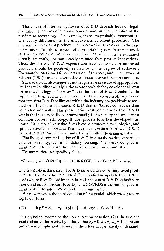
187 Tests of a Schumpeterian Model of R&D and Market Structure
The extent of interfirm spillovers of R&D depends both on legalinstitutional features of the environment and on characteristics of theproduct or technology. For example, there are probably important interindustry differences in the effectiveness of patent protection. Theinherent complexity of products and processes is also relevant to the easeof imitation. But these aspects of appropriability remain unmeasured.It is widely believed, however, that products, which can be examineddirectly by rivals, are more easily imitated than process innovations.Thus, the share of R&D expenditures devoted to new or improvedproducts .should be positively related to "I, the degree of spillovers.Fortunately, McGraw-Hill collects data of this sort, and recent work ofScherer (1981) presents alternative estimates derived from patent data.
Scherer's work also suggests another possible measure of appropriability. Industries differ widely in the extent to which they develop their ownprocess technology or "borrow" it in the form of R&D embodied incapital goods and intermediate products. It seems reasonable to presumethat interfirm R&D spillovers within the industry are positively associated with the share of process R&D that is "borrowed" rather thangenerated internally. This presumption rests on the idea that R&Dwithin the industry spills over more readily if the participants are using acommon process technology. If most process R&D is developed "inhouse," it is more likely that firms have idiosyncratic technologies, andspillovers are less important. Thus, we take the ratio of borrowed R&Dto total R&D "used" by an industry as another determinant of "I.
Finally, government funding of R&D frequently carries restrictionson appropriability, such as mandatory licensing. Thus, we expect government R&D to increase the extent of spillovers in an industry.
To summarize, we specify "I(e) as:
(26) "I == Co + Cl (PROD) + C2 (BORROW) + C3 (GOVRDS) + v,
where PROD is the share of R&D devoted to new or improved products, BORROW is the ratio of R&D embodied in inputs to total R&Dused (where R&D used by an industry is the sum of R&D embodied ininputs and its own process R&D), and GOVRDS is the ratio of government R&D to sales. We expect Cl, C2, and C3>0.
We now move to the third equation of the model, which we express inlog-linear form:
This equation resembles the concentration equation (21), in that themodel dictates the precise hypotheses that do == 0; d1 , d2 , d3 == 1. Here ourproblem is complicated because <p, the advertising elasticity of demand,
188 Richard C. Levin/Peter Ce Reiss
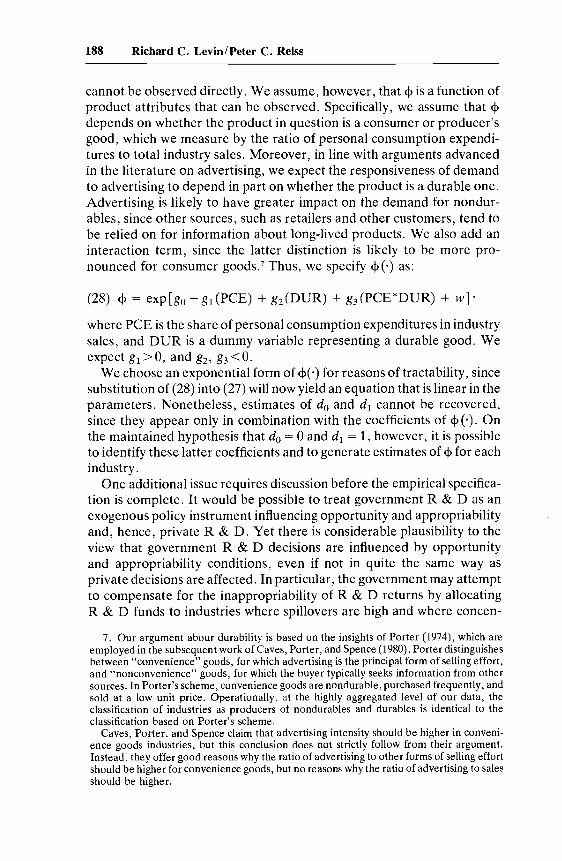
cannot be observed directly. We assume, however, that <f> is a function ofproduct attributes that can be observed. Specifically, we assume that <f>depends on whether the product in question is a consumer or producer'sgood, which we measure by the ratio of personal consumption expenditures to total industry sales. Moreover, in line with arguments advancedin the literature on advertising, we expect the responsiveness of demandto advertising to depend in part on whether the product is a durable one.Advertising is likely to have greater impact on the demand for nondurables, since other sources, such as retailers and other customers, tend tobe relied on for information about long-lived products. We also add aninteraction term, since the latter distinction is likely to be more pronounced for consumer goods. 7 Thus, we specify <f>(e) as:
(28) <f> = exp [go + gl (PCE) + g2 (DUR) + g3 (PCE*DUR) + w]'
where PCE is the share of personal consumption expenditures in industrysales, and DUR is a dummy variable representing a durable good. Weexpect gl > 0, and g2, g3 < o.
We choose an exponential form of <f>(e) for reasons of tractability, sincesubstitution of (28) into (27) will now yield an equation that is linear in theparameters. Nonetheless, estimates of do and d1 cannot be recovered,since they appear only in combination with the coefficients of <f> (e). Onthe maintained hypothesis that do = 0 and d1 = 1, however, it is possibleto identify these latter coefficients and to generate estimates of <f> for eachindustry.
One additional issue requires discussion before the empirical specification is complete. It would be possible to treat government R&D as anexogenous policy instrument influencing opportunity and appropriabilityand, hence, private R&D. Yet there is considerable plausibility to theview that government R&D decisions are influenced by opportunityand appropriability conditions, even if not in quite the same way asprivate decisions are affected. In particular, the government may attemptto compensate for the inappropriability of R&D returns by allocatingR&D funds to industries where spillovers are high and where concen-
7. Our argument abour durability is based on the insights of Porter (1974), which areemployed in the subsequent work of Caves, Porter, and Spence (1980). Porter distinguishesbetween "convenience" goods, for which advertising is the principal form of selling effort,and "nonconvenience" goods, for which the buyer typically seeks information from othersources. In Porter's scheme, convenience goods are nondurable, purchased frequently, andsold at a low unit price. Operationally, at the highly aggregated level of our data, theclassification of industries as producers of nondurables and durables is identical to theclassification based on Porter's scheme.
Caves, Porter, and Spence claim that advertising intensity should be higher in convenience goods industries, but this conclusion does not strictly follow from their argument.Instead, they offer good reasons why the ratio of advertising to other forms of selling effortshould be higher for convenience goods, but no reasons why the ratio of advertising to salesshould be higher.

189 Tests of a Schumpeterian Model of R&D and Market Structure
tration is low. This view receives support from the previous exploratorymodel of Levin (1981), where the hypothesis that GOVRDS is uncorrelated with the error term in the private R&D equation is decisivelyrejected in a test based on the work of Wu (1973), Hausman (1978), andReiss (1981). Although a truly satisfactory model of government R&Dallocation would give due weight to political forces, we observe that mostof the variance of government differences in R&D expenditures acrossindustries is explained by government procurement policy. Put simply,the government supports R&D in industries where it is a major customer; this holds especially for defense procurements. Therefore, wespecify that the ratio of government R&D to sales is determined by:
(29) GOVRDS = ho + hI (DEFSHR) + h2 (GOVSHR)
+ h3 H + (Mgl h3 + m OPPm )
+ C~l h3 + M + n APPn ) + e4,
where DEFSHR is the share of industry sales going to the federal government for defense purposes, and GOVSHR is the share of industry salespurchased by the federal government for other purposes.
8.4 The Data and Estimation Issues
Table 8.1 provides definitions, scalings, and the sources of the dataused in this study. Table 8.2 furnishes sample statistics for these data. Wehave already discussed in some detail the difficulties involved in measuring opportunity and appropriability and the rationale behind our measures. Most of the remaining variables are conventional and require nofurther comment (for further reference, see Levin 1981). We will, however, comment briefly on the measurement of R&D expenditures, priceelasticities of demand, and concentration before discussing estimationprocedures.
The only definitionally consistent industry R&D expenditure data arethose tabulated by the Bureau of the Census for the National ScienceFoundation (NSF). Unfortunately, they are only available for highlyagregated NSF industry classifications. Our sample consists of the twentybasic manufacturing industries for which data are available since 1963.These industries are a composite of four-, three-, and two-digit SICclassifications (see table 8.2). Since industry data on such variables asconcentration and the number of firms are only available for Census ofManufactures survey years (1963, 1967, and 1972), our sample consists ofsixty observations.
On the demand side, we use the price elasticities calculated by Levin

190 Richard C. Levin / Peter C. Reiss
Table 8.1 Variable Definitions and Data Sources
Variable Definition (data sources in parentheses)
HR
SRDINTGOVRDS
E
ELECCHEMBIOMECHMETBASICAGE
AGESQPROD
BORROW
PCEDURDEFSHR
GOVSHR
Herfindahl index of concentration (computed from COM)Company-financed R&D expenditures divided by value of shipments (NSF,COM)aAdvertising expenditures divided by industry output (10)Research intensity; RI(l - R - S)Government-financed R&D expenditures divided by value of shipments(NSF, COM)aPrice elasticity of demand (Almon, 10)Industry technology base predominantly electrical (scaled 0-1)Industry technology base predominantly chemical (scaled 0-1)Industry technology base predominantly biological (scaled 0-1)Industry technology base predominantly mechanical (scaled 0-1)Industry technology base predominantly metallurgical (scaled 0-1)Basic R&D expenditures divided by total R&D (NSF)Years since industry first appeared in Census of Manufactures with substantially same definition as today (COM)Square of AGEShare of industry R&D expenditures devoted to new or improved products(McGraw-Hill)R&D embodied in inputs divided by total R&D "used," where latter is thesum of own expenditures on process R&D and R&D embodied in inputs(Scherer)Personal consumption expenditures divided by industry sales (10)Dummy variable set equal to one for durable goods, zero otherwiseFederal government purchases for national defense purposes divided byindustry sales (I0)Federal government purchases for purposes other than national defensedivided by industry sales (10)
Key to Data Sources:Code SourceAlmon Almon, C., et al. 1974. 1985: Interindustry forecasts of the American
economy. Lexington, Mass.: Lexington Books.COM U.S. Bureau of the Census. 1963, 1967,1972. Census of manufactures.
Washington, D.C.: GPO.10 U.S. Department of Commerce, Bureau of Economic Analysis. 1963,
1967, 1972. Input-output tables for the United States. Washington, D.C.:GPO.
McGraw-Hill McGraw-Hill. Economics Department. Annual surveys ofbusiness plansfor research and development. Mimeo, annually.
NSF National Science Foundation, Research and development in industry.Washington, D.C.: GPO, annually.
Scherer Scherer, F. M. 1981. The structure of industrial technology flows. North-western University and FTC. Mimeo.
aR & D expenditure data were deflated by a salary index for chemists and engineersconstructed from data in U.S. Bureau of Labor Statistics, National Survey of Professional,Administrative, Technical, and Clerical Pay. Washington, D.C.: GPO, annually. Industryspecific employment weights for chemists and engineers were taken from BLS Bulletin no.1609, Scientific and Technical Personnel in Industry, 1961-66. Washington, D.C.: GPO,1968. Value of shipment data were deflated by use of sectoral output price deflators madeavailable on computer tape by the Bureau of Labor Statistics.

Tab
le8.
2Sa
mpl
eIn
dust
ries
,Se
lect
ed19
72D
ata,
and
Sam
ple
Stat
isti
cs
1972
Val
ues
ofS
elec
ted
Var
iabl
es
SIC
(196
7)In
dust
ryC
4H
RS
GO
VR
DS
20F
ood
and
kind
red
prod
ucts
36.0
62.0
023
.019
3.0
000+
22
,23
Tex
tile
prod
ucts
and
appa
rel
28.0
44.0
011
.006
0.0
000
24
,25
Lum
ber,
woo
dpr
oduc
ts,
and
furn
itur
e20
.030
.001
6.0
057
.000
026
Pap
eran
dal
lied
prod
ucts
31.0
50.0
067
.008
0.0
000+
281,
282
Indu
stri
alch
emic
als
45.1
02.0
298
.010
5.0
060
283
Dru
gs29
.043
.068
0.1
015
.000
228
4-28
9O
ther
chem
ical
s37
.063
.014
6.0
877
.000
629
Pet
role
umre
fini
ngan
dre
late
din
dust
ries
31.0
47.0
158
.011
5.0
005
30R
ub
ber
and
mis
cell
aneo
uspl
asti
cspr
oduc
ts31
.060
.011
1.0
155
.001
532
Sto
ne,
clay
,gl
ass,
and
conc
rete
prod
ucts
36.0
71.0
075
.007
5.0
001
331-
332,
3391
,33
99F
erro
usm
etal
san
dpr
oduc
ts41
.068
.003
8.0
029
.000
133
3-33
6,33
92N
onfe
rrou
sm
etal
san
dpr
oduc
ts49
.086
.004
8.0
043
.000
434
Fab
rica
ted
met
alpr
oduc
ts29
.055
.004
9.0
057
.000
235
Mac
hine
ry,
exce
ptel
ectr
ical
38.0
66.0
245
.004
4.0
053
366,
367
Com
mun
icat
ion
equi
pmen
tan
del
ectr
onic
com
pone
nts
45.0
92.0
963
.002
2.1
104
361-
365,
369
Oth
erel
ectr
ical
equi
pmen
t53
.110
.029
4.0
179
.024
937
1M
otor
vehi
cles
and
mot
orve
hicl
eeq
uipm
ent
81.2
51.0
263
.010
3.0
043
372
Air
craf
tan
dpa
rts
62.1
29.0
559
.002
1.2
385
381-
382
Sci
enti
fic
and
mec
hani
cal
mea
suri
ngin
stru
men
ts36
.059
.028
2.0
094
.006
838
3-38
7O
ptic
al,
surg
ical
,ph
otog
raph
ic,
and
othe
rin
stru
men
ts60
.123
.051
9.0
268
.014
2
Sam
ple
stat
isti
cs:
Mea
nov
eral
lin
dust
ries
and
year
s39
.6.0
78.0
247
.017
2.0
259
Sta
ndar
dde
viat
ion
14.1
.045
.023
7.0
253
.065
6M
inim
umva
lue
15.0
25.0
006
.001
0.0
000
Max
imum
valu
e81
.251
.096
3.1
015
.365
4

192 Richard C. LevinlPeter C. Reiss
(1981). These were computed using time-series estimates of constantelasticity demand functions made by Almon and his colleagues (1974).These estimates are available for fifty-six input-output sectors in whichthe predominant fraction of output goes to personal consumption. On therather strong pair of assumptions that all output in the fifty-six consumergoods sectors goes to personal consumption and that all output of theremaining maufacturing industries finds its way into consumer goodsindustries, derived elasticities of demand were calculated for each of theinput-output sectors in manufacturing. To the extent that some output ofthe fifty-six consumer goods industries is used as intermediate input or asinvestment goods and to the extent that some output of the remainingindustries is consumed directly, the calculated elasticities will be biased inuncertain direction and magnitude. Nevertheless, the procedure produces no serious anomalies; the relative magnitudes of the elasticitiesacross industries accord reasonably well with intuition.
The most difficult data problem we confront is to develop an operational analog of n, the number of firms. Obviously, the rather specialassumption of symmetric firm size is not consistent with the observedheterogeneity of firm sizes. Our approach here is to instead view n as anumbers equivalent (see, for example, Hart 1971) and to regard (22) asan approximation to a world with heterogeneous firm sizes. Our practicalproblem is how to summarize the empirical size distribution of firms by anumbers equivalent. For this purpose we choose to treat n as the Herfindahl numbers equivalent.
To obtain an operational measure, we must therefore construct aHerfindahl index for each sample industry. Since the empirical sizedistributions of firms are available in an incomplete form (e.g., C4, C8,C20, C50, etc.), we chose to fit two distributions (the Pareto and theexponential) to the available data for each four-digit industry. Of the twodistributions the exponential provided the more satisfactory approximation. Using the estimated parameters of these size distributions, wesimulated the Herfindahl index for each four-digit industry and then useda weighted average of four-digit Herfindahl indexes to represent concentration at the more aggregated level of our sample. The resulting indexvalues, which appear in table 8.2, are quite plausible. At the four-digitlevel, the correlation between the four-firm concentration ratio and ourestimated Herfindahl index is .91.
We now turn to estimation problems. While estimation of the advertising and concentration equations involves straightforward application ofnonlinear two-stage least-squares procedures, estimation of the R&Dequation is not straightforward. As noted above, the problem arisesbecause of the error in observing 'Y, which leads to a random coefficienton the concentration term, unless 'Y or e = 0, e = n, or (T~ = 0. That is,the system (22), (24), and (27) will not require attention to the random
193 Tests of a Schumpeterian Model of R&D and Market Structure
coefficient problem in three cases. (1) when 'Y or e = 0, firms behave asDasgupta-Stiglitz firms, and appropriability does not affect R&D intensity; (2) when e = n, concentration drops out of the R&D equation; and(3) if ~k is measured without error, no randomness is in the concentrationcoefficient.
The third of these special cases is the least probable. Thus, if we wish toestimate the model without prespecifying e, we must deal with theproblem of random coefficients in a nonlinear simultaneous equationscontext. To date, only Kelejian (1974) has suggested a procedure for thelinear simultaneous equations model with random coefficients, and forour model his specialized results are inapplicable.
Although we have not been able to find a fully efficient randomcoefficient estimator for our model, we are able to show that consistentestimates of the parameters in (24) can be obtained by nonlinear instrumental variables techniques. Details concerning the assumptions employed and a rigorous statement of this result are available from theauthors on request.
The more serious problem arising from the random coefficient versionof (24) is the possible inconsistency of conventional approximations tothe asymptotic standard errors of the coefficients. This inconsistencyresults from the heteroscedastic disturbance term. Our approach to thisproblem is to apply a generalized least-squares (GLS) correction to ourinstrumental variables estimator. To do this we must estimate a; and a~.
We do so by an auxiliary regression technique that uses the squaredresiduals from the initial instrumental variables estimates (see Hildrethand Houck 1968).
8.5 The Results
Table 8.3 summarizes the full specification of our four-equation model,along with the expected signs and parameter restrictions derived from theanalysis of section 8.3. All equations satisfy the conditions for identification of models involving nonlinearities in the endogenous variables. Weestimated each equation over our twenty industry sample for the years1963, 1967, and 1972. For each specification reported in this section wecould not reject the hypothesis of homogeneity across time periods. Wetherefore limit discussion to the results obtained using the pooled sample.
Each equation was estimated using single equation instrumental variables techniques involving linear approximations to the reduced forms.For the private R&D equation we attempted the Hildreth-Houck GLScorrection to take account of possible heteroscedasticity in the disturbance term. A decomposition of the residuals, however, revealed noevidence of heteroscedasticity. Furthermore, the GLS estimates andtheir standard errors were not much different from those obtained by the

194 Richard C. Levin/Peter C. Reiss
Table 8.3 Expected Signs and Magnitudes of Structural Coefficients
Variable LOG(H) RDINT LOG(S) GOVRDS
LOG(e) + 1.0 -1.0LOG(R + S) + 1.0LOG(H) + 1.0ELEC + +CHEM 7 7BIO 7MECH 7BASIC + +AGE +7 +7AGESQ -7 -7GOVRDS +H 7H*PROD +H*BORROW +H*GOVRDS +PCE +DURPCE*DURDEFSHR +GOVSHR +PROD +BORROW +CONSTANT 0.0 7 7 7
uncorrected instrumental variables procedure. For these reasons, weproceed as if (J"~ == 0, and we report the uncorrected parameter estimatesand standard errors in table 8.5 below.
Overall the results are quite encouraging given the small sample size,the degree of aggregation, and the potential measurement errors in ourdata. The signs of virtually all coefficients in the private R&D equationare in agreement with our predictions in table 8.3. Further, the pointestimates are remarkably robust to minor modifications in the specification, and many coefficients are significant at a size of .01. The results forthe concentration, advertising, and government R&D equations areless encouraging than those of the company R&D equation. Here thespecifications are quite sensitive to our implied restrictions. We nowproceed to a more detailed discussion of the results.
8.5.1 The Concentration Equation
Table 8.4 reports the results of estimating two variants of the concentration equation (21). Clearly, the estimated coefficients fail to conformto our precise predictions about their magnitudes. In specifications (4-1),we decisively reject the hypothesis that the constant is equal to zero, andthe strict hypotheses that al == a2 == 1 are also clearly rejected, separately
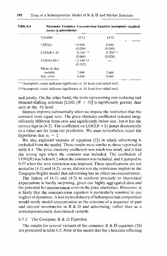
195 Tests of a Schumpeterian Model of R&D and Market Structure
Table 8.4 Parameter Estimates: Concentration Equation (asymptotic standarderrors in parentheses)
Variable (4-1)
LOG(E) -0.064(0.039)
LOG(R + S) 0.164***(0.068)
CONSTANT -2.146ttt(0.262)
Mean of dep.variable -2.666
Std. error 0.434
(4-2)
0.040(0.056)0.704***
(0.028)
-2.6660.660
***Asymptotic t-ratio indicates significance at .01 level (one-tailed test).
tttAsymptotic t-ratio indicates significance at .01 level (two-tailed test).
and jointly. On the other hand, the term representing cost-reducing anddemand-shifting activities [LOG (R + S)] is significantly greater thanzero at the .01 level.
Matters improve substantially when we impose the restriction that theconstant term equal zero. The price elasticity coefficient remains insignificantly different from zero and significantly below one, but it has thecorrect sign in (4-2). The coefficient on LOG(R + S) jumps dramaticallyto a value not far from our prediction. We must nevertheless reject thehypothesis that a2 == 1.
We also explored variants of equation (22) in which advertising isexcluded from the model. These results were similar to those reported intable 8.4. The price elasticity coefficient was much too small, and it hadthe wrong sign when the constant was included. The coefficient ofLOG(R) was below 0.2 when the constant was included, and it jumped to0.57 when the zero restriction was imposed. These specifications are notnested in (4-1) and (4-2), so we did not test the restriction implicit in theDasgupta-Stiglitz model that advertising has no effect on concentration.
The failure of (4-1) and (4-2) to conform precisely to theoreticalexpectations is hardly surprising, given our highly aggregated data andthe potential for measurement error in the price elasticities. Moreover, itis likely that the concentration equation is particularly sensitive to ourneglect of dynamics. A less stylized theory of Schumpeterian competitionwould surely model concentration as the outcome of a sequence of pastand current investments in R&D and advertising, rather than as acontemporaneously determined variable.
8.5.2 The Company R&D Equation
The results for several variants of the company R&D equation (24)are presented in table 8.5. Note at the outset that the 'Y function reflecting

196 Richard C. Levin/Peter C. Reiss
Table 8.5 Parameter Estimates: R&D Equation (asymptotic standard errorsin parentheses)
8, 'Y Unrestricted 'Y = Cons. 'Y, 8 = 0 8=n
Variable (5-1) (5-2) (5-3) (5-4) (5-5)
ELEC -0.038 0.017* 0.033*** 0.036*** 0.029***(0.027) (0.012) (0.011) (0.011) (0.012)
CHEM -0.006 -0.005 0.000 -0.001 -0.004(0.010) (0.007) (0.007) (0.007) (0.008)
BIO 0.064tt 0.060ttt 0.053tt 0.043t 0.038t(0.031) (0.022) (0.023) (0.022) (0.022)
MECH 0.004 0.009 0.017t 0.021tt 0.017t(0.014) (0.010) (0.010) (0.009) (0.010)
BASIC 0.101 0.259*** 0.299*** 0.349*** 0.358***(0.153) (0.100) (0.104) (0.098) (0.098)
AGE/100 0.152 -0.106t - 0.155tt - 0.147tt -0.121t(0.135) (0.064) (0.064) (0.066) (0.069)
AGESQ/100 -0.0016 0.0012t 0.0018tt 0.0017tt 0.OO15t(0.0015) (0.0007) (0.0007) (0.0007) (0.0008)
GOVRDS 2.694*** 0.078** 0.120*** 0.121*** 0.115***(1.005) (0.043) (0.042) (0.043) (0.043)
H -0.750tt - 0.362t 0.080(0.326) (0.205) (0.066)
H*PROD 1.715*** 0.742**(0.595) (0.328)
H*GOVRDS -24.082ttt(9.239)
PROD 0.034(0.031)
CONSTANT -0.054 0.009 0.020 0.021 0.008(0.033) (0.016) (0.016) (0.017) (0.030)
Mean of dep.variable 0.027 0.027 0.027 0.027 0.027
Std. error 0.022 0.016 0.017 0.017 0.017
*Asymptotic t-ratio indicates significance at .10 level (one-tailed test).
**Asymptotic t-ratio indicates significance at .05 level (one-tailed test).
***Asymptotic t-ratio indicates significance at .01 level (one-tailed test).
t Asymptotic t-ratio indicates significance at .10 level (two-tailed test).
ttAsymptotic t-ratio indicates significance at .05 level (two-tailed test).
tttAsymptotic t-ratio indicates significance at .01 level (two-tailed test).
the technological dimension of spillovers is modeled by including only aconstant term, PROD and GOVRDS, as arguments. Inclusion of bothPROD and BORROW in the regressions produced less satisfactoryresults, probably because of their near collinearity. Since PROD had themore robust parameter estimates over a range of specifications, we reportresults for variants of (24) omitting BORROW.
The most general form of (24) is where the value of eis arbitrary but

197 Tests of a Schumpeterian Model of R&D and Market Structure
constant across industries, as in (5-1) and (5-2). If R&D spillovers areassumed to be greater for products than for processes (i.e., PROD has apositive coefficient in the 'Y function), then the estimated coefficientsimply that eis greater than zero. Thus, firms appear to maintain positiveconjectural variations with respect to R&D, although the free-ridereffect could still be present if 0 < e < 1.
A somewhat surprising result of (5-1) is that the coefficient onH*GOVRDS is negative, suggesting that government funding diminishesspillovers. Although this contradicts our earlier expectation, the result isplausible for several reasons. Most prominently, much government funding supports R&D for large-scale, capital-intensive defense systemswhich are not cheaply replicable despite mandatory licensing and technology transfer provisions.
Specification (5-2) omits H*GOVRDS on the hypothesis that anotherreason for its unexpected sign may be its near collinearity with theopportunity vector. Once again, GOVRDS is significantly positive,although its effect on the cost elasticity is relatively small. The magnitudeof the coefficient indicates that on average a one dollar increase ingovernment R&D spending leads to a seven cent increase in companyR&D spending. Estimates for specifications (5-3) through (5-5) areabout eleven cents; however, at the means (5-1) yields a predicted effectof seventy-four cents. The other opportunity vatiables in (5-2) come instrongly with the correct signs.
Specifications (5-3) and (5-4) represent two restricted versions of (5-1)and (5-2). In (5-3) we test the hypothesis that 'Y is a constant across allindustries. The positive coefficient on the Herfindahl index indicates thateis greater than zero under the implicit assumption that 'Y is greater thanzero. In any case, Wald tests indicate that either (5-1) or (5-2) is to bepreferred to (5-3).
Specification (5-4) corresponds to a Dasgupta-Stiglitz world with noR&D spillovers. Interestingly enough, this equation does quite well inthat all the opportunity variables are of the correct sign and highlysignificant. Furthermore, the point estimates of the opportunity coefficients differ only slightly from those in (5-2). However, Wald tests onthe hypothesis that either 'Y or e equals zero lead to rejection of theDasgupta-Stiglitz model in favor of (5-1) or (5-2). The X2 statistics arerespectively X2(3) == 10.2 and X2(2) == 6.8.
The final specification we report is the "constant shares" case where eequals n and thus varies across industries. Once again the results accordreasonably well with the previous versions of the company R&D equation. Interestingly, we cannot reject the Dasgupta-Stiglitz model in favorof the constant shares case, given the insignificance of the coefficient ofPROD. Unfortunately, we are unable to test (5-5) against the otherversions, since (5-5) is not nested in the e, 'Y unrestricted cases.
Since it is widespread practice to treat concentration and government
198 Richard C. Levin/Peter C. Reiss
R&D as exogenous variables in empirical models of the determinationof company R&D, it is interesting to ask whether anything is gained bytreating them as endogenous. We checked for the possibility of simultaneity bias using the test proposed by Wu (1973). For each specificationin table 8.5, we decisively rejected the hypothesis that the regressors wetake to be stochastic were in fact uncorrelated with the disturbances.
As further checks on the models (5-1)-(5-5), we have tested the plausibility of our parameterization of a and the reasonableness of the opportunity measures. Operationally this was done by excluding the opportunity measures from all five equations. The resulting Wald statistics, whichare asymptotically distributed as X2 random variables with eight degreesof freedom, all exceeded the critical value at the .001 level. Thus, wedecisively reject the a constant version of the model.
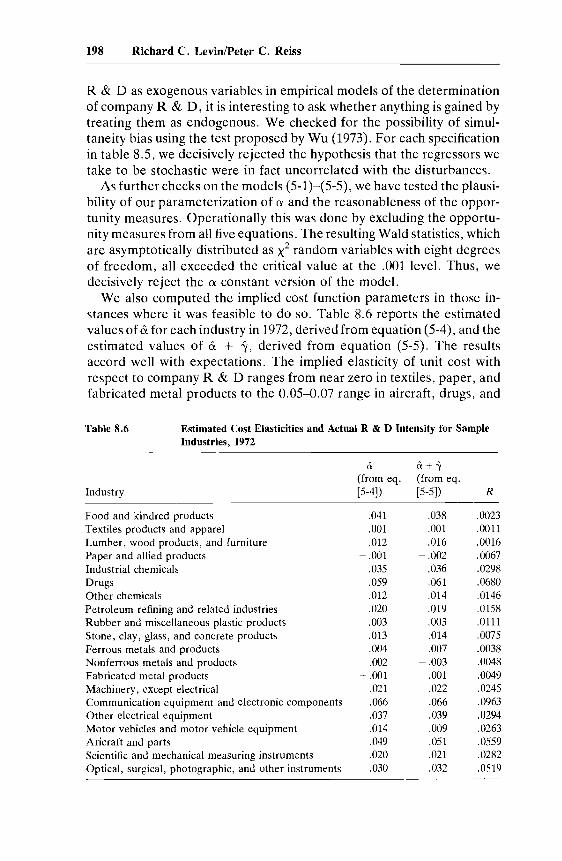
We also computed the implied cost function parameters in those instances where it was feasible to do so. Table 8.6 reports the estimatedvalues of &for each industry in 1972, derived from equation (5-4), and theestimated values of & + :V, derived from equation (5-5). The resultsaccord well with expectations. The implied elasticity of unit cost withrespect to company R&D ranges from near zero in textiles, paper, andfabricated metal products to the 0.05-0.07 range in aircraft, drugs, and
Table 8.6 Estimated Cost Elasticities and Actual R&D Intensity for SampleIndustries, 1972
Industry
Food and kindred productsTextiles products and apparelLumber, wood products, and furniturePaper and allied productsIndustrial chemicalsDrugsOther chemicalsPetroleum refining and related industriesRubber and miscellaneous plastic productsStone, clay, glass, and concrete productsFerrous metals and productsNonferrous metals and productsFabricated metal productsMachinery, except electricalCommunication equipment and electronic componentsOther electrical equipmentMotor vehicles and motor vehicle equipmentAricraft and partsScientific and mechanical measuring instrumentsOptical, surgical, photographic, and other instruments
&:(from eq.[5-4])
.041
.001
.012- .001
.035
.059
.012
.020
.003
.013
.004
.002-.001
.021
.066
.037
.014
.049
.020
.030
&:+-y(from eq.[5-5])
.038
.001
.016-.002
.036
.061
.014
.019
.003
.014
.007- .003
.001
.022
.066
.039
.009
.051
.021
.032
R
.0023
.0011
.0016
.0067
.0298
.0680
.0146
.0158
.0111
.0075
.0038
.0048
.0049
.0245
.0963
.0294
.0263
.0559
.0282
.0519
199 Tests of a Schumpeterian Model of R&D and Market Structure
electronics. Table 8.6 also includes the 1972 values ofR & D intensity forconvenient reference.
Finally, before turning to the advertising equation, we shall interpretthe coefficients on the industry age variables. The signs on the age andage-squared coefficients suggest that once an industry is defined by theCensus, it already faces declining opportunities for R&D. The magnitudes of these coefficients imply that opportunities decline for forty toforty-five years after definition, at which point they increase again. Depending on the specification, the standard error for the estimate of thisturning point is between five and six years.
8.5.3 The Advertising Equation
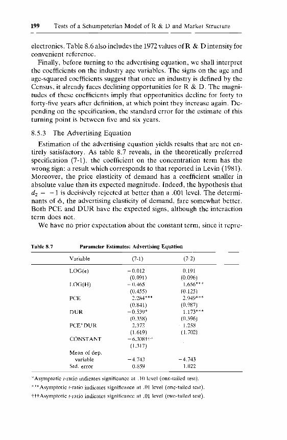
Estimation of the advertising equation yields results that are not entirely satisfactory. As table 8.7 reveals, in the theoretically preferredspecification (7-1), the coefficient on the concentration term has thewrong sign; a result which corresponds to that reported in Levin (1981).Moreover, the price elasticity of demand has a coefficient smaller inabsolute value than its expected magnitude. Indeed, the hypothesis thatd2 == -1 is decisively rejected at better than a .001 level. The determinants of <P, the advertising elasticity of demand, fare somewhat better.Both PCE and DUR have the expected signs, although the interactionterm does not.
We have no prior expectation about the constant term, since it repre-
Table 8.7 Parameter Estimates: Advertising Equation
Variable (7-1)
LOG(E) -0.012(0.091 )
LOG(H) - 0.465(0.455)
PCE 2.284***(0.841)
DUR - 0.539*(0.358)
PCE*DUR 2.373(1.619)
CONSTANT - 6.308ttt(1.317)
Mean of dep.variable -4.743
Std. error 0.859
(7-2)
0.191(0.096)1.656***
(0.125)2.949***
(0.987)1.173* **
(0.396)-1.258(1.702)
-4.7431.022
*Asymptotic [-ratio indicates significance at .10 level (one-tailed test).
***Asymptotic [-ratio indicates significance at .01 level (one-tailed test).
tttAsymptotic [-ratio indicates significance at .01 level (two-tailed test).
200 Richard C. Levin/Peter C. Reiss
sents the sum of do, which is expected to be zero, and d1gO, which involvesthe constant in the <t> function. If we constrain both do and go to be zero,however, the results improve markedly. The price elasticity coefficientreverses sign, but the remaining coefficients in (7-2) have the correctsigns. The concentration term is now significantly different from zero,although the hypothesis that d3 = 1 must be rejected at the .001 level.Each of the arguments of the <f> function now has the predicted sign, andthe hypothesis that <t>(.) is simply a constant across all industries can berejected for both specifications (7-1) and (7-2). In the former case, thehypothesis that <t> is a constant yields a test statistic that is X2(3) = 37.1. Inthe latter case, the test that <t> = 0 is X2(3) = 104.4.
The poor performance of the price elasticity variable in both this andthe concentration equation calls attention to the very strong assumptionsunder which the elasticities were computed. Some further work is neededhere; in future work we intend to employ alternative elasticity estimates.
8.5.4 The Government R&D Equation
As expected, the results in table 8.8 indicate that the allocation ofgovernment R&D expenditures is influenced most strongly by government defense procurement; the government supports R&D in thoseindustries in which it is a major customer. Technological opportunityappears to offer little incentive to the government; of our opportunitymeasures only AGE and AGESQ are statistically significant at conventionallevels. Interestingly, the signs of these coefficients are the reverseof those in most specifications of the private R&D equation. Given ourexpectation that the age profile proxies opportunity by first rising andthen falling, we might tentatively note that the pattern of signs in tables8.5 and 8.8 is consistent with the view that the government reacts totechnological opportunity with a substantial lag relative to private industry.
The technological dimension of spillovers, here proxied byBORROW, appears to have some effect on government R&D; asexpected, a higher degree of spillover increases the likelihood of government support. Again collinearity among the appropriability measuresleads to better results when either PROD or BORROW is excluded. Inthis case, BORROW has the more plausible parameter estimate and alower relative standard error. The structural dimension of appropriability, here represented by concentration, has the expected sign but fallswell short of statistical significance. The remaining coefficients in theequation are almost completely insensitive to the exclusion of this variable, as shown in (8-2). This suggests that GOVRDS is not strictlyendogenous, although its dependence on opportunity and appropriabilityconditions indicates that it is correlated with the error term in the private

201 Tests of a Schumpeterian Model of R&D and Market Structure
Table 8.8 Parameter Estimates: Government R&D Equation
Variable (8-1) (8-2)
ELEC 0.010 0.009(0.016) (0.014)
CHEM -0.003 -0.003(0.011) (0.010)
BIO 0.028 0.033(0.034) (0.031)
MECH 0.010 0.008(0.014) (0.012)
BASIC 0.012 0.015(0.159) (0.141)
AGE/100 0.224tt 0.220tt(0.099) (0.097)
AGESQ/100 -0.003tt -0.003tt(0.001) (0.001)
H -0.038(0.099)
BORROW 0.056** 0.053*(0.034) (0.032)
DEFSHR 0.066*** 0.066***(0.006) (0.006)
GOVSHR 0.001 0.002(0.048) (0.047)
CONSTANT - 0.072tt -0.071tt(0.030) (0.030)
Mean of dep.variable 0.026 0.026
Std. error 0.024 0.024
*Asymptotic t-ratio indicates significance at .10 level (one-tailed test).
**Asymptotic t-ratio indicates significance at .05 level (one-tailed test).
***Asymptotic t-ratio indicates significance at .01 level (one-tailed test).
ttAsymptotic t-ratio indicates significance at .05 level (two-tailed test).
R&D equation. Thus, the use of instrumental variables for GOVRDSseems appropriate.
8.6 Conclusions
Given the deficiencies of the variables used to measure technologicalopportunity and appropriability conditions, as well as the highly aggregated nature of the data, the results reported in section 8.5 are quiteencouraging. Although the statistical tests are not entirely consistent withour theoretical model, on the whole the findings support the Schumpeterian view that R&D investment and market structure are appropriately
202 Richard C. Levin/Peter C. Reiss
regarded as jointly determined outcomes of the competitive process. Theprivate R&D equation performs especially well, yielding results that arequite robust and yet sufficiently precise to reject decisively the hypotheses that opportunity and appropriability conditions do not matter. Indeed, the private R&D results are substantially better than thoseobtained in the looser, more inclusive, specification in the earlier work ofLevin (1981). The parameters of the concentration equation fail to conform to the precise predictions of our model, but the results neverthelesssuggest a strong and significant connection between cost-reducing anddemand-shifting activities and market concentration.
We do not wish to make exaggerated claims for our highly stylizedtheoretical model, which abstracts from obviously important features ofSchumpeterian competition, such as dynamics and the heterogeneity offirms. But we believe that the model does place proper emphasis ondemand, technological opportunity, and appropriability as the centralforces determining the allocation of R&D and the evolution of marketstructure. In particular, we believe our treatment of R&D spillovers,which distinguishes clearly the technological, structural, and behavioraldimensions of appropriability, exemplifies how useful insights may begained from relatively stark and stylized models. Moreover, our modelbrings to the foreground a thread linking much of the theoretical literature of the "new industrial organization": the endogeneity of marketstructure. Indeed, the recognition that market structure is endogenous isan element common to the literatures on Schumpeterian competition,monopolistic competition, strategic entry deterrence, and contestability.As these theoretical literatures continue to revise our understanding ofstructure-conduct-performance relationships, we will undoubtedly seemore empirical work of the type represented here.
It is well to keep in mind, however, both the strengths and weaknessesof empirical work based on highly stylized analytic models. On the onehand, such models have the virtue of simplicity, of clear and precisehypotheses. On the other hand, important features of reality are brushedaside. To this extent our insights are only partial truths.
The present paper exemplifies this dilemma. We have tested a simplemodel which captures much that is important. But a model of Schumpeterian competition without dynamics, without transient monopoly, withoutinnovators and imitators, is, at best, only part of the story. Much remainsto be done.
203 Tests of a Schumpeterian Model of R&D and Market Structure
References
Almon, C., M. B. Buckler, L. M. Horwitz, T. C. Reinhold 1974.1985:Interindustry forecasts of the American economy. Lexington, Mass.:Lexington Books.
Arrow, K. J. 1962. Economic welfare and the allocation of resources forinvention. In The rate and direction ofinventive activity: Economic andsocial factors, ed. R. R. Nelson. Universities-NBER ConferenceSeries no. 13. Princeton: Princeton University Press for the NationalBureau of Economic Research.
Caves, R. E., M. E. Porter, and A. M. Spence. 1980. Competition in theopen economy. Cambridge: Harvard University Press.
Dasgupta, P., and J. E. Stiglitz. 1980a. Industrial structure and thenature of innovative activity. Economic Journal 90:266-93.
---. 1980b. Uncertainty, industrial structure, and the speed ofR&D. Bell Journal of Economics 11:1-28.
Dorfman, R., and P. O. Steiner. 1954. Optimal advertising and optimalquality. American Economic Review 44:826-36.
Farber, S. 1981. Buyer market structure and R&D effort: A simultaneous equations model. Review of Economics and Statistics 63:33645.
Fellner, W. J. 1951. The influence of market structure on technologicalprogress. Quarterly Journal of Economics 65:556-77.
Futia, C. 1980. Schumpeterian competition. Quarterly Journal of Economics 94:675-95.
Galbraith, J. K. 1956. American capitalism: The concept ofcountervailingpower. 2d ed. Boston: Houghton Mifflin.
Hart, P. E. 1971. Entropy and other measures of concentration. Journalof the Royal Statistical Society, series A, 134:73-85.
Hausman, J. A. 1978. Specification tests in econometrics. Econometrica46:1251-71.
Hildreth, C., and J. P. Houck. 1968. Some estimators for a linear modelwith random coefficients. Journal of the American Statistical Association 63:584-95.
Kamien, M., and N. Schwartz. 1975. Market structure and innovation: Asurvey. Journal of Economic Literature 13:1-37.
Kelejian, H. H. 1974. Random parameters in a simultaneous equationframework: Identification and estimation. Econometrica 42:517-27.
Lee, T., and L. L. Wilde. 1980. Market structure and innovation: Areformulation. Quarterly Journal of Economics 94:429-36.
Levin, R. C. 1978. Technical change, barriers to entry, and marketstructure. Economica 45:347-61.
---. 1981. Toward an empirical model of Schumpeterian competi-

204 Richard C. Levin/Peter C. Reiss
tion. Working paper series A, no. 43. Yale School of Organization andManagement.
Loury, G. C. 1979. Market structure and innovation. Quarterly Journalof Economics 93:395-410.
Nelson, R. R. 1959. The simple economics of basic scientific research.Journal of Political Economy 67:297-306.
---. 1981. Balancing market failure and governmental inadequacy.Working paper. Yale University.
Nelson, R. R., and S. G. Winter. 1977. Dynamic competition and technical progress. In, Economic progress, private values and public policy:Essays in honor of William Fellner, ed. B. Balassa and R. R. Nelson.Amsterdam: North-Holland.
---. 1978. Forces generating and limiting concentration underSchumpeterian competition. Bell Journal of Economics 9:524-48.
---. 1982. The Schumpeterian trade-off revisited. American Economic Review 72:114-32.
Phillips, A. 1966. Patents, potential competition, and technical progress.American Economic Review 56:301-10.
---. 1971. Technology and market structure: A study of the aircraftindustry. Lexington, Mass.: Lexington Books.
Porter, M. E. 1974. Consumer behavior, retailer power, and marketperformance in consumer goods industries. Review of Economics andStatistics 56:419-35.
Reiss, P. 1981. Small and large sample equivalences of Hausman's m teststo the classical specification tests. Working paper. Yale University.
Scherer, F. M. 1965. Firm size, market structure, opportunity, and theoutput of patented inventions. American Economic Review 55:10971125.
---. 1967. Market structure and the employment of scientists andengineers. American Economic Review 57:524-31.
---. 1980. Industrial market structure and economic performance. 2ded. Chicago: Rand-McNally.
---. 1981. The structure of industrial technology flows. NorthwesternUniversity and FTC. Mimeo.
Schumpeter, J. A. 1950. Capitalism, socialism, and democracy. 3d ed.New York: Harper and Row.
Wu, D. 1973. Alternative tests of independence between stochastic regressors and disturbances. Econometrica 41:733-50.

205 Tests of a Schumpeterian Model of R&D and Market Structure
Comment Pankaj Tandon
This is an interesting paper, since it seeks to initiate the difficult task ofbuilding bridges between recent theoretical work on R&D and theempirical work on this subject, of which we have seen many fine examplesat this conference. I welcome this bridge-building activity, but believe, asthe authors do, that much remains to be done. I will therefore concentrate my remarks on the general modeling approach and on some of theproblems that need special attention.
The authors are obviously aware of many of the modeling problemsinvolved here, and they have commented on several. I will reemphasizeonly one-the question of timing. When one considers timing, it isprobable-as the authors point out-that the effect of technologicalchange on market structure is a long-term effect, one that cannot beeasily captured in tests that span only ten years. Seen in this light, it is notsurprising that the concentration equation fails to be convincing. On theother hand, the influence of market structure on R&D investmentdecisions is more likely to be captured in a short panel. As a short-runapproximation, it is probably reasonable to assume a fixed market structure. Thus, the relative success of the R&D intensity equation was alsoto be expected.
Let me comment on what the authors mention as the two majorcontributions of their approach. The first relates to the inclusion ofadvertising as another variable influencing and being influenced by market structure. Though the authors comment on the similarity betweenadvertising and R&D as instruments of competition, they treat them inquite an asymmetric manner in their model. Specifically, the way advertising is included is to model the aggregate industry demand curve asdepending on the aggregate level of advertising in the industry. Thus, ifthere are n firms in the industry, any firm doing advertising gets in effectonly l/nth of the increase in demand. Clearly this does not really capturethe competitive characteristics of advertising; rather, advertising acquiresthe characteristics of a public good-with a serious attendant free-riderproblem. The corresponding treatment for R&D would be to say that afirm's unit cost is a function only of Z (aggregate industry R&D). Thisdoesn't seem reasonable. Likewise, I don't find the treatment of advertising convincing. The results from the advertising equation are not satisfactory in any case and might be better explained by a story that concentrated on the role of advertising in product differentiation. I don't know ifI'm just revealing my bias as someone primarily interested in R&D, butI think I'd be happier with advertising left out of the model. Another
Pankaj Tandon is an assistant professor in the Department of Economics, BostonUniversity.

206 Richard C. Levin/Peter C. Reiss
reason for this is that it is far from clear to me that R&D and advertisingare jointly determined. In a model with uncertain R&D outcomes,advertising may be sequentially determined, conditioned on the results ofR&D.
Since the primary interest of this group is R&D, let me move on to thesecond, more interesting point, namely, the model of R&D spillovers.This is surely welcome. The public goods aspect of R&D has receivedinsufficient attention in the theoretical and empirical literature , yet it isone of the things that makes R&D particularly interesting and distinctfrom traditional investment. I am, however, a little uncomfortable withthe way spillovers have been modeled here. The authors have taken theunit cost of production to be a function of the firm's own R&D and ofaggregate industry R&D. I have two problems with this. First, as isclearly evidenced by Professor Scherer's work on interindustry technology flows, spillovers are also important across industries. This will be ofspecial importance when, as the authors promise us, more disaggregateddata at the four-digit level are used. Further, such cross-industry externalities may be quite important in determining market structure in userindustries. Two obvious examples spring to mind. The development ofsmall, powerful computers will surely be important, although it is notclear whether the major influence will be to increase or decrease concentration. It seems that minimum efficient scale may be significantly reduced in many industries. On the other hand, small computers maycombine with the second example, improved telecommunications capabilities, to considerably ease the control problem in large corporations.This would clearly tend to increase concentration. Some attention mustbe paid to these interindustry externalities.
The second problem with the spillover analysis concerns the logicalconsistency of the model. All firms in an industry are assumed to face thesame technological opportunities. We then concentrate on symmetricequilibria. In the absence of uncertainty, the only logical interpretation ofsuch an equilibrium is that every firm has discovered the same things. Butthen, why should the R&D of other firms be of any value to me, since Ialready know what they know? (In fact, this logic would say that the onlypermissible spillovers would be interindustry!) I grant that a model withasymmetric information and uncertainty-even with symmetry-is goingto be analytically much less tractable, and it is not obvious that theestimable equations would be structurally different, but I do worry aboutthe logical anomaly.
The spillovers were nevertheless an interesting addition to the model,particularly because of a side product that was generated. Including Z inthe cost function enabled the authors to begin to model different behavioral hypotheses about firms, specifically: What are firms' conjecturesabout the response of their rivals to their own R&D? Unfortu-
207 Tests of a Schumpeterian Model of R&D and Market Structure
nately, the authors are not able to get clear answers on this, mainlybecause the conjectural parameter e appears multiplicatively with theappropriability parameter 'Y. I have two suggestions. First, Z could bemeasured excluding the firm's own R&D. This seems conceptuallypreferable anyway, although I grant that at this level of aggregation itmay not appear important. However, the interpretation of ewill be quitedifferent and, in particular, its sign will matter. Now e = 0 will correspond to the Cournot conjecture, ewill be negative for free-rider situations, and e will be positive for what might be called Schumpeterianconjectures. Under the assumption that 'Y is positive, it will be possible torun tests on the sign of e. In the present version, eis always positive, and itis not possible to find its magnitude distinctly from 'Y. Of course, equation(13) would have to be modified-the n in the denominator would have tobe replaced by (n - I)-and perhaps other things would change in themodel. The second suggestion is that perhaps a model that pays moreexplicit attention to product differentiation may be more successful anddesirable. In other words, we might get more directly at the conjecturalhypotheses by thinking about the firm's demand or price being influencedby other firms' costs.
A specific comment here: In regression (5-4), the R&D equation forthe Dasgupta-Stiglitz case, the authors do not tell us if the left-hand sidewas modified to be RI(l - R). Advertising surely ought to be excluded ifthe equation is to represent the Dasgupta-Stiglitz model.
I have a couple of other brief comments. We have not seen theconditions that ensure the existence of symmetric equilibria, but we caneasily guess the parameters that must appear there. Since it is well knownthat R&D causes nonconvexities, it is of some interest to make sure thatthe existence conditions are being satisfied. It would be useful if theauthors provided that information. Further, since ex, the elasticity of unitcost with respect to R&D, is estimable in their model, it would be usefulto report it and to compare it with the many other estimates of thisparameter or its variants that exist in the literature.
One noticeable feature of this paper is how distinct it is methodologically from other papers presented at this conference. I think it may beuseful for the authors in their bridge-building activity to look again at thework of Pakes and Schankerman (this volume) on the determinants ofresearch intensity. This is perhaps the clearest exposition of the traditional approach, and it might be productive to attempt to modify thisapproach with an endogenous market structure.
Finally, let me say what I think is most attractive about this line ofwork. The significant way in which the endogenous market structureapproach differs from the traditional approach is that the new approachintroduces a zero-profit condition. This corresponds to what Scherer, inthe context of the optimal patent literature, has called the Lebensraum

208 Richard C. Levin/Peter C. Reiss
effect. I think that it is entirely possible that this Lebensraum effectactually is the dominant consideration in R&D allocations, especiallybecause of the serious possibility of nonconvexities. Consideration of theLebensraum effect might also have implications for patent policy orantitrust. For example, some very crude Harberger-type calculations thatI have done indicate that in industries where technological opportunity ishigh, the optimal market structure may be quite concentrated, preciselybecause of the Lebensraum effect. The trade-off between static anddynamic efficiency is very explicit in Schumpeter's work, and theapproach of Levin and Reiss is a first step toward the integration of thistrade-off into empirical work on R&D.