Quantitative microscopy and colocalisationanalysis using ImageJ

Colin Rickman (colin.rickman@ed.ac.uk)Beyond pretty pictures - Second workshop series about the basics of light microscopy

Outline of workshop

• What does colocalisation mean• Qualitative colocalisation• Quantitative colocalisation• Hands-on examples (in HRB room 253)

Colocalisation

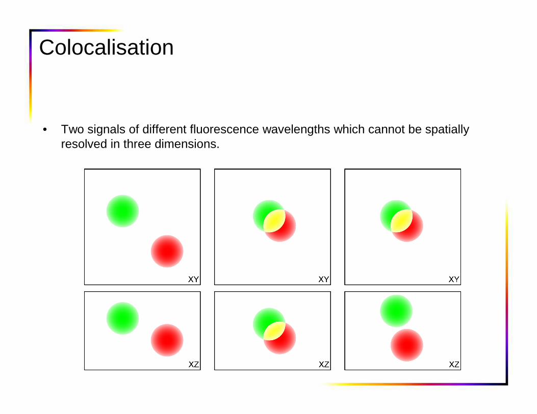
• Two signals of different fluorescence wavelengths which cannot be spatially resolved in three dimensions.

Colocalisation

• Two signals of different fluorescence wavelengths which cannot be spatially resolved in three dimensions.

Colocalisation

• Two signals of different fluorescence wavelengths which cannot be spatially resolved in three dimensions.

– Colocalisation analysis requires a three-dimensional data set, properly acquired and restored based on the psf.

• Can be used wherever you want to test if two fluorophores are occuying the same part of the cell.

• It does not say they are interacting. Can only be indirectly inferred through perturbation of an interaction.

• Ultimately limited by the resolution of the microscope.

Qualitative colocalisation

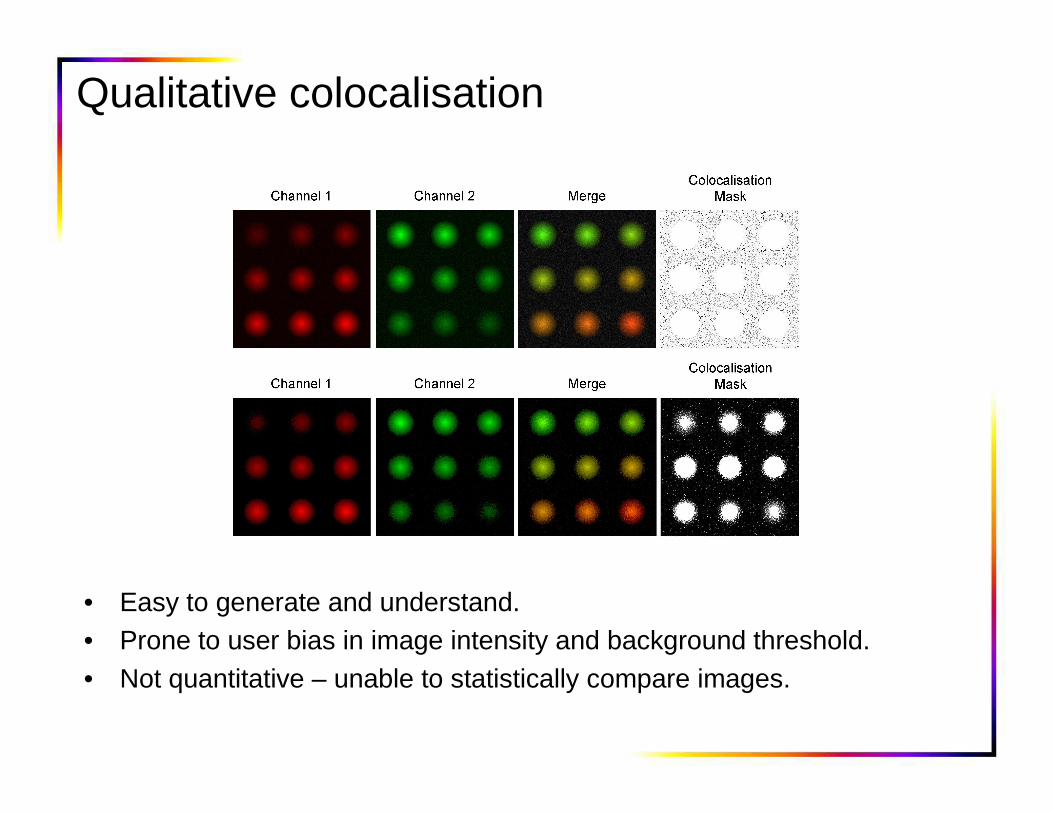
• Easy to generate and understand.• Prone to user bias in image intensity and background threshold.• Not quantitative – unable to statistically compare images.

Qualitative colocalisation

• Easy to generate and understand.• Prone to user bias in image intensity and background threshold.• Not quantitative – unable to statistically compare images.

Quantitative colocalisation

• Overlap coefficient– Ranges from low (0) to high (1) colocalisation.

– Requires a similar number of pixels in each channel and a user defined background threshold.

• Manders coefficients– Provides, on a range from low (0) to high (1), information on colocalisation of

channel 1 with channel 2 and vice versa.

– Very sensitive to background threshold and does not provide information on relative intensities in each pixel.

• Pearson’s correlation coefficient– A measure of correlation between the intensities of each channel in each pixel.– Multiple experiments can be combined or compared.– No spatial information.

– No user defined background threshold.

• Residual map– A graphical presentation of an image based on the linear regression used to

calculate the Pearson’s correlation coefficient.

– No user defined background threshold.

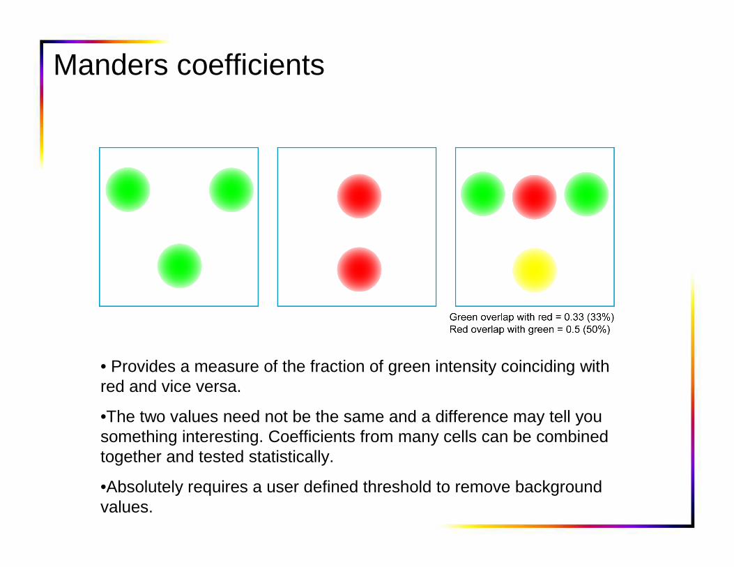
Manders coefficients

• Provides a measure of the fraction of green intensity coinciding with red and vice versa.

•The two values need not be the same and a difference may tell you something interesting. Coefficients from many cells can be combined together and tested statistically.

•Absolutely requires a user defined threshold to remove background values.

Manders coefficients

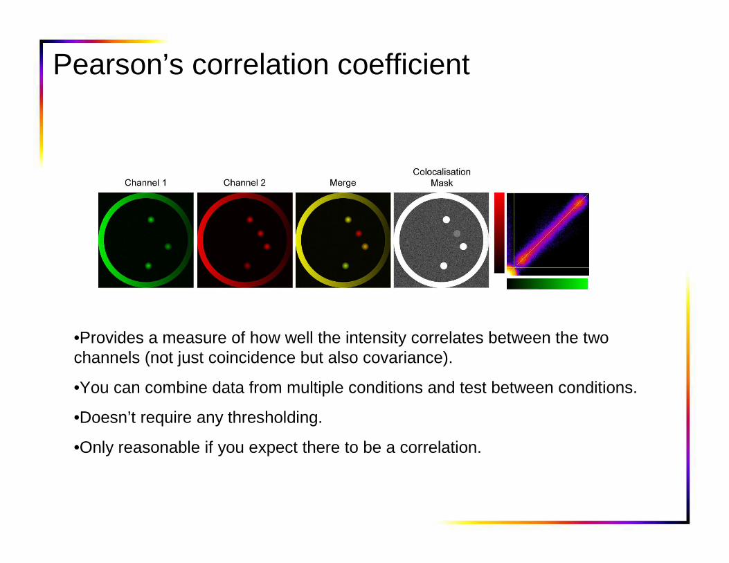
Pearson’s correlation coefficient

•Provides a measure of how well the intensity correlates between the two channels (not just coincidence but also covariance).

•You can combine data from multiple conditions and test between conditions.

•Doesn’t require any thresholding.

•Only reasonable if you expect there to be a correlation.

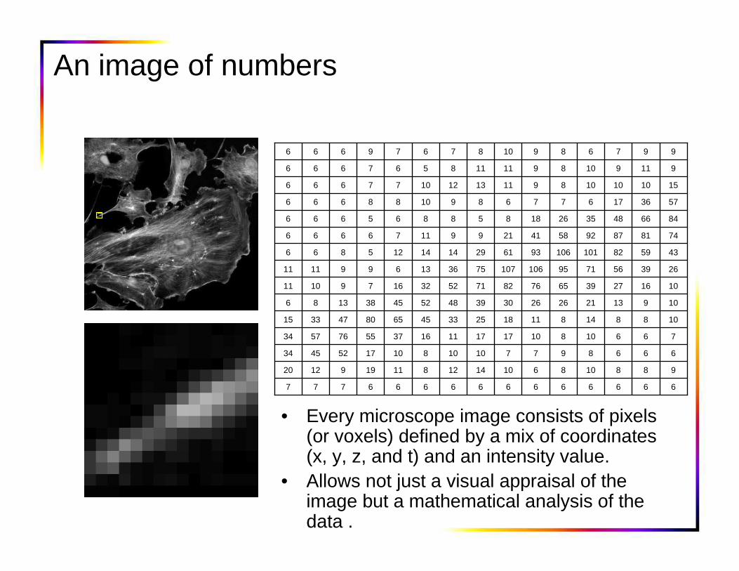
An image of numbers

666666666666777

98810861014128111991220

6668977101081017524534

76610810171711163755765734

108814811182533456580473315

109132126263039485245381386

1016273965768271523216791011

26395671951061077536136991111

4359821011069361291414125866

74818792584121991176666

846648352618858865666

5736176776891088666

15101010891113121077666

9119108911118567666

9976891087679666

• Every microscope image consists of pixels (or voxels) defined by a mix of coordinates (x, y, z, and t) and an intensity value.

• Allows not just a visual appraisal of the image but a mathematical analysis of the data .

Pearson’s correlation coefficient

Combining multiple data sets of Pearson’s correlation coefficients

• Comparison of Pearson’s correlation coefficients between conditions for multiple cells.

• Allows for the effect of cell to cell variation to be minimised.• Comparison with an experimental control condition provides a baseline

for the experiment.

Correlation and residual mapping

• A residual map is a way to present the information on covarianceprovided by Pearson’s in a spatial way.

• Deviation from the linear regression (the residual) is shown on a colour scale from -1 to +1 with zero residual coloured cyan.Does not require user defined thresholds.

Correlation and residual mapping in live cells

Where to get help

• Impact and Calm imaging facilities managers• Me (colin.rickman@ed.ac.uk)• The McMaster Biophotonics Facility ImageJ website

(http://www.macbiophotonics.ca/imagej/)• The ImageJ website (http://rsbweb.nih.gov/ij/index.html)• The ImageJ wiki (http://imagejdocu.tudor.lu/)• The ImageJ mailing list (http://rsbweb.nih.gov/ij/list.html)

• All material is available at http://tinyurl.com/impact-teaching(Username: impactoutreach / Password: impactoutreach)