HAL Id hal-00609176httpshal-supelecarchives-ouvertesfrhal-00609176

Submitted on 26 Jul 2012

HAL is a multi-disciplinary open accessarchive for the deposit and dissemination of sci-entific research documents whether they are pub-lished or not The documents may come fromteaching and research institutions in France orabroad or from public or private research centers

Lrsquoarchive ouverte pluridisciplinaire HAL estdestineacutee au deacutepocirct et agrave la diffusion de documentsscientifiques de niveau recherche publieacutes ou noneacutemanant des eacutetablissements drsquoenseignement et derecherche franccedilais ou eacutetrangers des laboratoirespublics ou priveacutes

Quantitative functional failure analysis of athermal-hydraulic passive system by means of

bootstrapped Artificial Neural NetworksEnrico Zio George Apostolakis Nicola Pedroni

To cite this versionEnrico Zio George Apostolakis Nicola Pedroni Quantitative functional failure analysis of a thermal-hydraulic passive system by means of bootstrapped Artificial Neural Networks Annals of Nuclear En-ergy Elsevier Masson 2010 37 (5) pp639-649 lt101016janucene201002012gt lthal-00609176gt

1

Quantitative functional failure analysis of a thermal-hydraulic

passive system by means of bootstrapped

Artificial Neural Networks

E Zioa G E Apostolakisb N Pedronia aEnergy Department Politecnico di Milano Via Ponzio 343 20133 Milan Italy

Phone +39-2-2399-6340 fax +39-2-2399-6309 E-mail address enricoziopolimiit

bDepartment of Nuclear Science and Engineering Massachusetts Institute of Technology

77 Massachusetts Avenue Cambridge (MA) 02139-4307 Phone +1-617-252-1570 fax +1-617-258-8863

E-mail address apostolamitedu

Abstract The estimation of the functional failure probability of a thermal-hydraulic (T-H) passive system can

be done by Monte Carlo (MC) sampling of the epistemic uncertainties affecting the system model

and the numerical values of its parameters followed by the computation of the system response by a

mechanistic T-H code for each sample The computational effort associated to this approach can

be prohibitive because a large number of lengthy T-H code simulations must be performed (one for

each sample) for accurate quantification of the functional failure probability and the related

statistics

In this paper the computational burden is reduced by replacing the long-running original T-H

code by a fast-running empirical regression model in particular an Artificial Neural Network

(ANN) model is considered It is constructed on the basis of a limited-size set of data representing

examples of the inputoutput nonlinear relationships underlying the original T-H code once the

model is built it is used for performing in an acceptable computational time the numerous system

response calculations needed for an accurate failure probability estimation uncertainty

propagation and sensitivity analysis

The empirical approximation of the system response provided by the ANN model introduces an

additional source of (model) uncertainty which needs to be evaluated and accounted for A

bootstrapped ensemble of ANN regression models is here built for quantifying in terms of

confidence intervals the (model) uncertainties associated with the estimates provided by the ANNs

For demonstration purposes an application to the functional failure analysis of an emergency

passive decay heat removal system in a simple steady-state model of a Gas-cooled Fast Reactor

2

(GFR) is presented The functional failure probability of the system is estimated together with

global Sobol sensitivity indices The bootstrapped ANN regression model built with low

computational time on few (eg 100) data examples is shown capable of providing reliable (very

near to the true values of the quantities of interest) and robust (the confidence intervals are

satisfactorily narrow around the true values of the quantities of interest) point estimates

1 Introduction

Passive systems (IAEA 1991) are expected to contribute significantly to the safety of future nuclear

power plants by combining their peculiar characteristics of simplicity reduction of human

interaction (Prosek and Cepin 2008) and reduction or avoidance of hardware failures (Mathews et

al 2008) On the other hand the uncertainties associated to their actual operation and modelling

are usually larger than in active systems

Two different sources of uncertainties are usually considered in safety analyses randomness due to

intrinsic variability in the behavior of the system (aleatory uncertainty) and imprecision due to lack

of data on some underlying phenomena (eg natural circulation) and to scarce or null operating

experience over the wide range of conditions encountered during operation (epistemic uncertainty)

(Apostolakis 1990 Helton 2004)

Due to these uncertainties there is a nonzero probability that the physical phenomena involved in

the operation of a passive system do not occur as expected thus leading to the failure of performing

the intended safety function even if safety margins have been dimensioned (Marquegraves et al 2005

Patalano et al 2008)

Various methodologies have been proposed in the open literature to quantify the probability that T-

H passive systems fail to perform their functions the reader is referred to (Burgazzi 2007 Zio and

Pedroni 2009a) for a review A reasonable approach to take is that founded on the concept of

functional failures in the framework of reliability physics and load-capacity exceedance probability

(Burgazzi 2003) In this view a passive system fails to perform its function due to deviations from

its expected behavior which lead the load imposed on the system (eg the peak value of the fuel

cladding temperature during a LOCA transient) to overcome its capacity (eg a threshold value

imposed by regulating authorities or by the mechanical properties of structural materials) This

concept is at the basis of many works of literature including (Jafari et al 2003 Marquegraves et al

2005 Pagani et al 2005 Bassi and Marquegraves 2008 Mackay et al 2008 Mathews et al 2008 and

2009 Patalano et al 2008 Fong et al 2009 Zio and Pedroni 2009a and b) in these works the

passive system is modeled by a detailed mechanistic T-H system code and the probability of not

performing the required function is estimated based on a Monte Carlo (MC) sample of code runs

3

which propagate the epistemic (state-of-knowledge) uncertainties in the model describing the

system and the numerical values of its parametersvariables because of these uncertainties the

system may not accomplish its mission even if no hardware failure occurs

MC simulation allows a realistic assessment of the T-H system functional failure probability thanks

to its flexibility and indifference to the complexity of the T-H model This however is paid in

terms of the high computational efforts required Indeed a large number of Monte Carlo-sampled

T-H model evaluations must generally be carried out for an accurate estimation of the functional

failure probability Since the number of simulations required to obtain a given accuracy depends on

the magnitude of the failure probability to be estimated with the computational burden increasing

with decreasing functional failure probability (Schueller 2007) this poses a significant challenge

for the typically quite small (eg less than 10-4) probabilities of functional failure of T-H passive

safety systems In particular the challenge is due to the time required for each run of the detailed

mechanistic T-H system code which can take several hours (one code run is required for each

sample of values drawn from the uncertainty distributions of the input parametersvariables to the

T-H code) (Fong et al 2009) Thus alternative methods must be sought to tackle the computational

burden associated to the analysis

To tackle the computational issue efficient sampling techniques can be adopted for obtaining robust

estimations with a limited number of input samples Techniques like Importance Sampling (IS) (Au

and Beck 2003 Schueller et al 2004) Stratified Sampling (Helton and Davis 2003 Cacuci and

Ionescu-Bujor 2004) and Latin Hypercube Sampling (LHS) (Helton and Davis 2003) have been

widely used in reliability analysis and risk assessment (Helton 1998) Recently advanced sampling

methods such as Subset Simulation (SS) (Au and Beck 2001 Au and Beck 2003) and Line

Sampling (LS) (Koutsporelakis et al 2004 Pradlwarter et al 2005) have been proposed for

structural reliability assessment and subsequently applied to the estimation of the functional failure

probability of a T-H passive system (Zio and Pedroni 2009a and b)1 These methods have been

shown to improve the computational efficiency although there is no indication yet that the number

of model evaluations can be reduced to below a few hundreds which may be mandatory in the

presence of computer codes requiring several hours to run a single simulation

1 Apart from efficient MC techniques there exist methods based on nonparametric order statistics (Wilks 1942) that propagate uncertainties through mechanistic T-H codes with reduced computational burden especially if only one- or two-sided confidence intervals are needed for particular statistics (eg the 95th percentile) of the outputs of the code For example the so-called coverage (Guba et al 2003 Makai and Pal 2006) and bracketing (Nutt and Wallis 2004) approaches can be used to identify the precise number of sample code runs required to obtain a given confidence level on the estimates of prescribed statistics of the code outputs

4

In such cases the only viable alternative seems that of resorting to fast-running surrogate

regression models also called response surfaces or meta-models to approximate the inputoutput

function implemented in the long-running T-H model code and then substitute it in the passive

system functional failure analysis The construction of such regression models entails running the

T-H model code a predetermined reduced number of times (eg 50-100) for specified values of the

uncertain input parametersvariables and collecting the corresponding values of the output of

interest then statistical techniques are employed for fitting the response surface of the regression

model to the inputoutput data generated in the previous step Several examples can be found in the

open literature concerning the application of surrogate meta-models in reliability problems In

(Bucher and Most 2008 Gavin and Yau 2008 Liel et al 2008) polynomial Response Surfaces

(RSs) are employed to evaluate the failure probability of structural systems in (Arul et al 2009

Fong et al 2009 Mathews et al 2009) linear and quadratic polynomial RSs are employed for

performing the reliability analysis of T-H passive systems in advanced nuclear reactors in (Deng

2006 Hurtado 2007 Cardoso et al 2008 Cheng et al 2008) learning statistical models such as

Artificial Neural Networks (ANNs) Radial Basis Functions (RBFs) and Support Vector Machines

(SVMs) are trained to provide local approximations of the failure domain in structural reliability

problems in (Volkova et al 2008 Marrel et al 2009) Gaussian meta-models are built to calculate

global sensitivity indices for a complex hydrogeological model simulating radionuclide transport in

groundwater

In this work Artificial Neural Networks (ANNs) are considered to reduce the computational burden

associated to uncertainty propagation in the functional failure analysis of a natural convection-based

decay heat removal system of a Gas-cooled Fast Reactor (GFR) (Pagani et al 2005) A limited-size

set of inputoutput data examples is used to construct the ANN regression model once the model is

built it is used to perform in a negligible computational time the functional failure analysis of the

T-H passive system in particular the functional failure probability of the system is estimated

together with global sensitivity indices of the naturally circulating coolant temperature

The use of regression models in safety critical applications like nuclear power plants raises concerns

with regards to the model accuracy which must be not only verified but also quantified in this

paper we resort to the bootstrap method for quantifying in terms of confidence intervals the model

uncertainty associated to the estimates provided by ANNs (Efron and Thibshirani 1993) Some

examples of the application of the bootstrap method for the evaluation of the uncertainties

associated to the output of regression models in safety-related problems can be found in the

literature in (Zio 2006) bootstrapped ANNs are trained to predict nuclear transients processes in

5

(Cadini et al 2008 Secchi et al 2008) the model uncertainty quantified in terms of a standard

deviation is used to ldquocorrectrdquo the ANN output in order to provide conservative estimates for

important safety parameters in nuclear reactors (ie percentiles of the pellet cladding temperature)

finally in (Storlie et al 2008) the bootstrap procedure is combined with different regression

techniques eg Multivariate Adaptive Regression Spline (MARS) Random Forest (RF) and

Gradient Boosting Regression (GBR) to calculate confidence intervals for global sensitivity indices

of the computationally demanding model of a nuclear waste repository

The main objective of the present study is to show the possibility of

bull limiting the computational burden associated to the uncertainty propagation and sensitivity

analyses underpinning a quantitative functional failure analysis of a T-H passive system to

this aim ANN regression models trained on a small data set are used for the first time for

the estimation of

the functional failure probability of the passive system

first-order global Sobol sensitivity indices determining the contribution of the

individual uncertain parameters (ie the inputs to the T-H code) to the uncertainty in

the coolant temperature (ie the output of the T-H code) and consequently to the

probability of functional failure of the passive system

bull quantifying in terms of confidence intervals the model uncertainty associated to the

estimates of the functional failure probability and Sobol indices provided by the ANN

models To the best of the authorsrsquo knowledge the issue of quantification of model

uncertainty in the regression estimates has not been addressed in the literature regarding the

functional failure analysis of T-H passive systems (Arul et al 2009 Fong et al 2009

Mathews et al 2009) in the present work bootstrapped ANNs are used to the purpose

The paper organization is as follows In Section 2 the concepts of functional failure analysis for T-

H passive systems are synthetically summarized Section 3 briefly presents the problem of empirical

regression modeling by means of ANNs and provides a snapshot on the bootstrap method for the

quantification of the ANN (model) uncertainty In Section 4 the case study of literature concerning

the passive cooling of a GFR is presented In Section 5 the results of the application of

bootstrapped ANNs to the functional failure analysis of the T-H passive system of Section 4 are

reported Conclusions are provided in the last section Finally algorithmic details about the

bootstrap-based method for quantifying in terms of confidence intervals the model uncertainty

6

associated to the estimates of safety parameters computed by ANN regression models are reported

in the Appendix at the end of the paper

2 Functional failure analysis of T-H passive systems

Since a comprehensive functional failure analysis of a T-H passive system is beyond the scope of

this work only the essential steps for the conceptual development of the analysis are briefly

reported below (Marquegraves et al 2005)

1 Define the failure criteria of the passive system

2 Build a deterministic best-estimate T-H model to simulate the passive system behavior

3 Identify and characterize by proper probability distributions the factors of uncertainty in the

results of the best estimate T-H calculations In the present work only epistemic

uncertainties are considered due to the limited knowledge on some phenomena and

processes (eg models parameters and correlations used in the T-H analysis)

4 Propagate by Monte Carlo Simulation (MCS) the epistemic uncertainties associated to the

identified relevant parameters models and correlations (step 3 above) through the

deterministic long-running T-H code in order to estimate the functional failure probability

of the passive system conditional on the current state of knowledge about the phenomena

involved (step 3 above) (Bassi and Marques 2008 Mackay et al 2008 Mathews et al

2008 Patalano et al 2008) Formally let x = x1 x2 hellip xj hellip inx be the vector of the

relevant uncertain system parametersvariables Y( x ) be a scalar indicator variable of the

performance of the passive system (eg the fuel peak cladding temperature) and αY a

threshold value defining the corresponding failure criterion (eg a limit value imposed by

regulating authorities) For illustrating purposes let us assume that the passive system

operates as long as Y( x ) lt αY The MCS procedure for estimating the functional failure

probability entails that a large number NT of samples of the values of the system parameters

x be drawn from the corresponding probability distributions and used to evaluate Y(x) by

running the T-H code An estimate ( )P F of the probability of failure P(F) can then be

computed by dividing the number of times that Y( x ) gt αY by the total number of samples

NT

5 Perform a sensitivity study to determine the contribution of the individual uncertain

parameters (ie the inputs to the T-H code) to the uncertainty in the outputs of the T-H code

and consequently to the functional failure probability of the T-H passive system As is true

for uncertainty propagation (step 4 above) sensitivity analysis relies on multiple

evaluations of the code for different combinations of system inputs

7

The computational burden posed by the uncertainty propagation and sensitivity analysis of steps 4

and 5 above may be tackled by replacing the long-running original T-H model code by a fast-

running surrogate regression model properly built to approximate the output from the true system

model In this paper Artificial Neural Networks (ANNs) (Bishop 1995) are used A confidence

interval is evaluated by means of the bootstrap method (Efron and Thibshirani 1993) a brief

description of this latter technique is given in the following Section whereas the relevant

algorithmic details can be found in the Appendix at the end of the paper

3 Bootstrapped Artificial Neural Networks for empiric al regression

modelling

As discussed in the previous Section the computational burden posed by uncertainty and sensitivity

analyses of T-H passive systems can be tackled by replacing the long-running original T-H model

code by a fast-running surrogate regression model Because calculations with the surrogate model

can be performed quickly the problem of long simulation times is circumvented

Let us consider a generic meta-model to be built for performing the task of nonlinear regression

ie estimating the nonlinear relationship between a vector of input variables x = x1 x2 xj

inx and a vector of output targets y = y1 y2 yl ony on the basis of a finite (and possibly

reduced) set of inputoutput data examples (ie patterns) ( ) trainpptrain NpD 21 == yx (Zio

2006) It can be assumed that the target vector y is related to the input vector x by an unknown

nonlinear deterministic function ( )xmicroy corrupted by a noise vector ( )xε ie

( ) ( ) ( )xεxmicroxy y += (1)

Notice that in the present case of T-H passive system functional failure probability assessment the

vector x contains the relevant uncertain system parametersvariables the nonlinear deterministic

function ( )xmicroy represents the complex long-running T-H mechanistic model code (eg RELAP5-

3D) the vector y(x) contains the output variables of interest for the analysis and the noise ( )xε

represents the errors introduced by the numerical methods employed to calculate ( )xmicroy (Storlie et

al 2008) for simplicity in the following we assume ( )xε = 0 (Secchi et al 2008)

The objective of the regression task is to estimate ( )xmicroy in (1) by means of a regression function

f(x w) depending on a set of parameters w to be properly determined on the basis of the available

data set Dtrain the algorithm used to calibrate the set of parameters w is obviously dependent on the

nature of the regression model adopted but in general it aims at minimizing the mean (absolute or

8

quadratic) error between the output targets of the original T-H code yp = ( )pymicro x p = 1 2

Ntrain and the output vectors of the regression model ( )ˆ wxfy pp = p = 1 2 Ntrain for

example the Root Mean Squared Error (RMSE) is commonly adopted to this purpose (Zio 2006)

( )2

1 1

1ˆ

train oN n

p l p lp ltrain o

RMSE y yN n = =

= minussdot sumsum (2)

Once built the regression model f(x w) can be used as a simplified quick-running surrogate of the

original long-running T-H model code for significantly reducing the computational burden

associated to the accurate estimation and epistemic uncertainty propagation steps of the functional

failure analysis of T-H passive systems In particular the regression model f(x w) can be used in

place of the T-H code to calculate any quantity of interest Q eg the functional failure probability

of the passive system confidence intervals and global sensitivity indices etc

In this work three-layered feed-forward Artificial Neural Network (ANN) regression models are

considered In extreme synthesis ANNs are computing devices inspired by the function of the nerve

cells in the brain (Bishop 1995) They are composed of many parallel computing units (called

neurons or nodes) interconnected by weighed connections (called synapses) Each of these

computing units performs a few simple operations and communicates the results to its neighbouring

units From a mathematical viewpoint ANNs consist of a set of nonlinear (eg sigmoidal) basis

functions with adaptable parameters w that are adjusted by a process of training (on many different

inputoutput data examples) ie an iterative process of regression error minimization (Rumelhart et

al 1986) The details about ANN regression models are not reported here for brevity the interested

reader may refer to the cited references and the copious literature in the field The particular type of

ANN employed in this paper is the classical three-layered feed-forward ANN trained by the error

back-propagation algorithm

When using the approximation of the system output provided by an ANN empirical regression

model an additional source of uncertainty is introduced which needs to be evaluated particularly in

safety critical applications like those related to nuclear power plant technology One way to do this

by resorting to bootstrapped ANN regression models (Efron and Thibshirani 1993) ie an

ensemble of ANN regression models constructed on different data sets bootstrapped from the

original one (Zio 2006 Storlie et al 2008) The bootstrap method is a distribution-free inference

method which requires no prior knowledge about the distribution function of the underlying

population (Efron and Thibshirani 1993) The basic idea is to generate a sample from the observed

data by sampling with replacement from the original data set (Efron and Thibshirani 1993) From

the theory and practice of ensemble empirical models it can be shown that the estimates given by

9

bootstrapped ANN regression models is in general more accurate than the estimate of the best ANN

regression model in the bootstrap ensemble of ANN regression models (Zio 2006 Cadini et al

2008)

A bootstrap-based estimation technique is here employed for the evaluation of the so-called

Bootstrap Bias Corrected (BBC) point estimate ˆBBCQ of a generic quantity Q (eg a safety

parameter) by an ANN regression model f(x w) and the calculation of the associated BBC

Confidence Interval (CI) (Zio 2006 Storlie et al 2008) The complete algorithm is not reported

here for brevity some details can be found in the Appendix at the end of the paper

4 Case study functional failure analysis of a T-H passive system

The case study considered in this work concerns the natural convection cooling in a Gas-cooled

Fast Reactor (GFR) under a post-Loss Of Coolant Accident (LOCA) condition (Pagani et al 2005)

The reactor is a 600-MW GFR cooled by helium flowing through separate channels in a silicon

carbide matrix core whose design has been the subject of study in the past several years at the

Massachussets Institute of Technology (MIT) (Pagani et al 2005)

In these studies the possibility of using natural circulation to remove the decay heat in case of an

accident is demonstrated In particular in the case of a LOCA the long-term heat removal is

ensured by natural circulation in a given number Nloops of identical and parallel loops

A GFR decay heat removal configuration is shown schematically in Figure 1 only one of the Nloops

loops is reported for clarity of the picture the flow path of the cooling helium gas is indicated by

the black arrows the loop has been divided into Nsections = 18 sections for numerical calculation

technical details about the geometrical and structural properties of these sections are not reported

here for brevity the interested reader may refer to (Pagani et al 2005)

Figure 1 here

In the present analysis the average core power to be removed is assumed to be 187 MW

equivalent to about 3 of full reactor power (600 MW) to guarantee natural circulation cooling at

this power level a pressure of 1650 kPa is required in nominal conditions Finally the secondary

side of the heat exchanger (ie item 12 in Figure 1) is assumed to have a nominal wall temperature

of 90 degC (Pagani et al 2005)

The model describes the quasi-steady-state natural circulation cooling that takes place after the

LOCA transient has occurred The associated simplifications introduced in the modeling allow

relatively fast calculations which enable to obtain reference values for comparison of the estimates

10

obtained by the ANN models developed From a strictly mathematical point of view obtaining a

steady-state solution amounts to dropping the time dependent terms in the energy and momentum

conservation equations In practice the T-H model code balances the pressure losses around the

loops so that friction and form losses are compensated by the buoyancy term while at the same time

maintaining the heat balance in the heater (ie the reactor core item 4 in Figure 1) and cooler (ie

the heat exchanger item 12 in Figure 1) a thorough description of the deterministic T-H model is

not given here for brevity the interested reader may refer to (Pagani et al 2005) for details

41 Uncertainties in the T-H model

Uncertainties affect the actual operation of passive systems and its modeling On the one side there

are phenomena like the occurrence of unexpected events and accident scenarios eg the failure of

a component or the variation of the geometrical dimensions and material properties which are

random in nature This kind of uncertainty in the model description of the system behavior is

termed aleatory (NUREG-1150 1990 Helton 1998 USNRC 2002) In this work as well as in the

reference paper by (Pagani et al 2005) aleatory uncertainties are not considered for the estimation

of the functional failure probability of the T-H passive system of Figure 1

An additional contribution of uncertainty comes from the incomplete knowledge on the properties

of the system and the conditions in which the phenomena occur (ie natural circulation) This

uncertainty is often termed epistemic and affects the model representation of the system behaviour

in terms of both (model) uncertainty in the hypotheses assumed and (parameter) uncertainty in the

values of the parameters of the model (Cacuci and Ionescu-Bujor 2004 Helton et al 2006

Patalano et al 2008)

Model uncertainty arises because mathematical models are simplified representations of real

systems and therefore their outcomes may be affected by errors or bias It may for example

involve the correlations adopted to describe the T-H phenomena which are subject to errors of

approximation Such uncertainties may for example be represented by a multiplicative model (Zio

and Apostolakis 1996 Patalano et al 2008)

)( ζsdot= xmz (3)

where z is the real value of the parameter to be correlated (eg heat transfer coefficients friction

factors Nusselt numbers or thermal conductivity coefficients) m() is the mathematical model of

the correlation x is the vector of correlating variables and ζ is a multiplicative error factor Hence

the uncertainty in the output quantity z is translated into an uncertainty in the multiplicative error

factor ζ commonly classified as representing model uncertainty

11

Uncertainty affects also the values of the parameters used in the model (eg power level pressure

cooler wall temperature material conductivity hellip) eg owing to errors in their measurement or

insufficient data and information As a consequence the values of such parameters are usually

known only to a certain level of precision ie epistemic uncertainty is associated with them

(Pagani et al 2005)

In this work only epistemic (ie model and parameter) uncertainties are represented and

propagated through the deterministic T-H code (Pagani et al 2005 Bassi and Marques 2008

Mackay et al 2008 Mathews et al 2008 Patalano et al 2008) Parameter uncertainties are

associated to the reactor power level the pressure in the loops after the LOCA and the cooler wall

temperature Model uncertainties are associated to the correlations used to calculate the Nusselt

numbers and friction factors in the forced mixed and free convection regimes The corresponding

nine uncertain inputs of the model 129jx j = are assumed to be distributed according to

normal distributions of known mean micro and standard deviation σ taking values in the range [micro - 4σ micro

+ 4σ] (Table 1 Pagani et al 2005) The practical and conceptual reasons underpinning the values in

Table 1 are described in (Pagani et al 2005)

Table 1 here

42 Failure criteria of the T-H passive system

The passive decay heat removal system of Figure 1 is considered failed whenever the temperature

of the coolant helium leaving the core (item 4 in Figure 1) exceeds either 1200 degC in the hot channel

or 850 degC in the average channel these values are expected to limit the fuel temperature to levels

which prevent excessive release of fission gases and high thermal stresses in the cooler (item 12 in

Figure 1) and in the stainless steel cross ducts connecting the reactor vessel and the cooler (items

from 6 to 11 in Figure 1) (Pagani et al 2005)

Indicating by x the vector of the 9 uncertain system parameters of Table 1 (Section 41) and by

( )xhotcoreoutT and ( )xavg

coreoutT the coolant outlet temperatures in the hot and average channels

respectively the failure event F can be written as follows

( ) ( ) 8501200 gtcupgt= xxxx avgcoreout

hotcoreout TTF (4)

Notice that in the notation of the preceding Section 3 ( )xhotcoreoutT = y1(x) and ( )xavg

coreoutT = y2(x) are

the two target outputs of the T-H model

The failure event F in (4) can be condensed into a single performance indicator Y(x) (Section 2) as

12

( ) ( ) ( ) ( ) ( )

=

=850

1200850

1200

21 xxxxx

yymax

TTmaxY

avgcoreout

hotcoreout (5)

so that the failure event F becomes specified as

( ) 1 gt= xx YF (6)

In the notation of Section 2 the failure threshold αY is then equal to one

5 Results of the application of bootstrapped ANNs for the functional

failure analysis of the T-H passive system of Section 4

In this Section the results of the application of bootstrapped Artificial Neural Networks (ANNs) for

the quantitative functional failure analysis of the 600-MW GFR passive decay heat removal system

in Figure 1 are illustrated First few details about the construction of the ANN regression model are

given in Section 51 then this is used to estimate the probability of functional failure of the system

(Section 52) finally the sensitivity of the hot-channel coolant outlet temperature to the uncertain

input parameters is studied by computing first-order Sobol indices (Section 53) Notice that at each

estimation step the model uncertainties associated to the above mentioned quantities are also

estimated by bootstrapping the ANN regression models (see Section 3 and the Appendix)

51 Building and testing the ANN regression model

The ANN model used in this work is built using a set ( ) trainpptrain NpD 21 == yx of

inputoutput data examples of size Ntrain = 100 this is done to test the capability of the ANN

regression model to reproduce the outputs of the nonlinear T-H model code on the basis of a

relatively small number of runs from the original T-H code A Latin Hypercube Sample (LHS) of

the inputs is drawn to give the vectors xp = x1p x2p hellip xjp hellip in px p = 1 2 hellip Ntrain (Zhang

and Foschi 2004) Then the original T-H model is evaluated on the input vectors xp p = 1 2 hellip

Ntrain to obtain the corresponding output vectors yp = microy(xp) = y1p y2p ylp on py p = 1 2

hellip Ntrain and build the data set ( ) trainpptrain NpD 21 == yx Finally the adjustable parameters

w of the ANN regression model are calibrated to fit the generated data in particular the common

error back-propagation algorithm is implemented to train the ANN (Rumelhart et al 1986)

In the present case study the number ni of inputs to the ANN regression model is equal to 9 (ie

the number of uncertain inputs in Table 1 of Section 41) whereas the number no of outputs is equal

to 2 (ie the number of system variables of interest the hot- and average-channel coolant outlet

temperatures as reported in Section 42) The number of nodes nh in the hidden layer has been set

equal to 4 by trial and error

13

A validation data set ( ) 12 20val p p valD p N= = =x y (different from the training set Dtrain) is

used to monitor the accuracy of the ANN model during the training procedure in practice the

RMSE (2) is computed on Dval at different phases of the training procedure At the beginning the

RMSE computed on the validation set Dval typically decreases together with the RMSE computed

on the training set Dtrain then when the ANN regression model starts overfitting the data the

RMSE calculated on the validation set Dval starts increasing this is the time to stop the training

algorithm

For a realistic measure of the ANN model accuracy the widely adopted coefficient of determination

2R and the RMSE have been computed for each output yl l = 1 2 no on a new data set

( ) testpptest NpD 21 == yx also of size Ntest = 20 not used during training (Marrel et al 2009)

Table 2 reports the values of the coefficient of determination 2R and of the RMSE associated to the

estimates of the hot- and average- channel coolant outlet temperatures hotcoreoutT and avg

coreoutT

respectively computed on the test set Dtest of size Ntest = 20 by the ANN model with nh = 4 hidden

neurons built on a data set Dtrain of size Ntrain = 100 the number of adjustable parameters (ANN

weights) w in the ANN regression model is also reported

Table 2 here

The large values of the coefficient of determination R2 ie 09897 and 09866 and the small values

of 12 degC and 63 degC for the RMSEs produced by the ANN for the hot- and average-channel coolant

outlet temperatures hotcoreoutT and avg

coreoutT respectively lead us to assert that the accuracy of the ANN

model can be considered satisfactory for the needs of estimating the functional failure probability of

the present T-H passive system

Finally in order to demonstrate that the trial-and-error selected ANN architecture with nh = 4

hidden neurons is suitable for the present application Table 2 contains also the values of the

coefficient of determination 2R and of the RMSE associated to the estimates of the hot- and

average- channel coolant outlet temperatures hotcoreoutT and avg

coreoutT respectively obtained on the test

set Dtest by two additional ANN topologies in particular ANN regression models with nh = 3 and 5

hidden neurons are considered It can be seen that the values of the coefficient of determination R2

obtained by the ANN architecture with nh = 3 hidden neurons are 09821 and 09763 (ie lower

than those produced by the ANN with nh = 4 hidden neurons) while the values of the RMSEs are

160 degC and 85 degC (ie larger than those produced by the ANN with nh = 4 hidden neurons) for the

14

hot- and average-channel coolant outlet temperatures hotcoreoutT and avg

coreoutT respectively The values

of the coefficient of determination R2 obtained by the ANN architecture with nh = 5 hidden neurons

are 09891 and 09860 (again lower than those produced by the ANN with nh = 4 hidden neurons)

while the values of the RMSEs are 134 degC and 76 degC (again larger than those produced by the

ANN with nh = 4 hidden neurons) for the hot- and average-channel coolant outlet temperatures

hotcoreoutT and avg

coreoutT respectively

52 Functional failure probability estimation

In this Section the bootstrapped ANNs are used for estimating the functional failure probability

and associated confidence interval of the 600-MW GFR passive decay heat removal system of

Figure 1 The previous system configuration with Nloops = 3 is analyzed

Table 3 reports the value of the Bootstrap Bias Corrected (BBC) estimate ( )BBCFP of the functional

failure probability (per demand) P(F) obtained with NT = 500000 estimations from B = 1000

bootstrapped ANNs built on Ntrain = 100 data examples the corresponding Bootstrap Bias Corrected

(BBC)-95 Confidence Interval (CI) is also reported A ldquotruerdquo value of the functional failure

probability P(F) is also reported in Table 3 for reference (ie P(F) = 334middot10-4) this has been

obtained with a very large number NT (ie NT = 500000) of simulations of the original T-H code

which actually runs fast enough to allow repetitive calculations (one code run lasts on average 3

seconds on a Pentium 4 CPU 300GHz) the computational time required by this reference analysis

is thus 500000middot3 s = 1500000 s asymp 417 h

Table 3 here

It can be seen that bootstrapped ANNs are quite reliable because the value of the BBC point

estimate ( )BBCFP (ie 359middot10-4) is quite close to the ldquotruerdquo value (ie 334middot10-4) of the functional

failure probability P(F) In spite of the small value of the failure probability (ie P(F) ~ 10-4) this is

done by resorting to quite a low number of runs of the T-H code (ie only Ntrain + Nval + Ntest = 100

+ 20 + 20 = 140 inputoutput examples for training validating and testing the bootstrapped ANN

model)

In addition the BBC-95 CI produced by the bootstrapped ANNs provides a measure of the

(model) uncertainty associated to the ANN point estimate ( )BBCFP this information is particularly

interesting when very few data are used to build the bootstrapped ANN models and consequently

15

the confidence of the analyst in the obtained BBC point estimate ( )BBCFP is poor In this respect

the upper bound of the BBC-95 CI (in this case 412middot10-4) can be used to provide a slightly

conservative estimate of the corresponding functional failure probability P(F) Note that the BBC-

95 CI includes the ldquotruerdquo value of P(F) (ie 334middot10-4) and it is quite narrow around it this

confirms the robustness of the estimates produced by the trained bootstrapped ANN regression

models in the present application

Finally a computational time of about 2 hours is associated to the calculation of the BBC point

estimate ( )BBCFP for P(F) and the corresponding BBC-95 CI (Table 3) this value includes the

time required for i) generating the Ntrain + Nval + Ntest = 100 + 20 + 20 = 140 inputoutput examples

by running the T-H code (ie on average 140middot3 s = 420 s = 7 m asymp 012 h) ii) training the

bootstrapped ensemble of B = 1000 ANN models by means of an error back-propagation algorithm

(ie on average 2 h) and iii) performing NT = 500000 evaluations of each of the B = 1000

bootstrapped ANN models (ie on average 6 minutes = 01 h) The overall CPU time required by

the use of bootstrapped ANNs (ie on average 222 h) is about 180 times lower than that required

by the use of the original T-H model code (ie on average 417 h)

53 Global sensitivity analysis based on first-order Sobol indices

In the functional failure analysis of a T-H passive system sensitivity analysis is a useful tool for

identifying the uncertain parameters (ie the uncertain inputs to the T-H code) that contribute most

to the variability of the model outputs (ie the coolant outlet temperatures) In the following first-

order Sobol sensitivity indices are computed only for the hot-channel coolant outlet temperature

hotcoreoutT by way of example (Sobol 1993)

By definition the first-order Sobol sensitivity index Sjl j = 1 2 hellip ni l = 1 2 hellip no quantifies the

proportion of the variance of the output yl l = 1 2 hellip no that can be attributed to the variance of

the uncertain input variable xj alone ie without taking into account interactions with other input

variables It is formally defined as

( )[ ]

| 12 12j jx l jl

j i ol

V E y xS j n l n

V yminus

= = =

x (7)

where V[yl] is the variance of the model output yl l = 1 2 hellip no obtained when all model input

parameters xj j = 1 2 hellip ni are sampled over their variation range 1 2 1 1 ij j j nx x x x xminus minus +=x

is a vector containing all the uncertain input variables except xj and ( )|j jx l jV E y x

minus x is the

expected variance of yl obtained when the input parameter of interest xj is fixed and all the

16

remaining input variables are sampled over their variation ranges a thorough description of this

sensitivity measure goes far beyond the scope of this work further details can be found in (Saltelli

2002a)

As pointed out in (Saltelli 2002b) the sensitivity index (7) has the advantage of being global

because the effect of the entire distribution of the parameter whose uncertainty importance is

evaluated is considered moreover this sensitivity index is also ldquomodel freerdquo because its

computation is independent from assumptions about the model form such as linearity additivity

and so on The drawback of this approach relies in the computational burden associated to its

calculation Actually if N samples (ie T-H model code evaluations) are used to calculate both the

expected value ( )|j l jE y x

minusx and the variance ( )|j jx l jV E y x

minus x in (7) by crude Monte Carlo

sampling then the total number NT of samples required to compute (7) is NT = N2 for each output yl

of interest l = 1 2 hellip no (Saltelli et al 2008) for example if N = 102 divide 103 then NT = 104 divide 106

rendering impracticable the associated analysis The total number NT of samples can be reduced to

N(ni + 2) by resorting to an efficient algorithm proposed by (Saltelli 2002b) in this case if N = 102

divide 103 and ni = 9 (like in the present problem) then NT = 11middot103 divide 11middot104 leading to a reduction of

one or two orders of magnitude in the number of required T-H code simulations details about these

algorithms can be found in the cited references

In this work the hot channel coolant outlet temperature hotcoreoutT = y1 is chosen as output of interest

for the analysis and the algorithm proposed by (Saltelli 2002b) has been implemented with N =

10000 and ni = 9 (ie NT = 110000) to obtain the ldquotruerdquo (ie reference) values of the first-order

Sobol sensitivity indices 1jS for the input variables xj j = 1 2 hellip 9 The reference ranking of the

uncertain input variables obtained with NT = 110000 runs of the original T-H model code is reported

in the left column of Table 4 together with the corresponding values of the first-order Sobol

sensitivity indices 1jS j = 1 2 hellip 9 (in parentheses) The Table also shows the ranking of the

uncertain input parameters xj j = 1 2 hellip 9 based on the BBC point estimates 1

ˆj BBCS j = 1 2 hellip

9 obtained with NT = 110000 estimations from B = 1000 bootstrapped ANN models built on Ntrain =

100 inputoutput data examples (right column) finally the computational time (in hours) associated

to both analyses (ie on average 92 h and 212 h respectively) is also reported on a Pentium 4

CPU 300GHz

Table 4 here

17

It can be seen that the ranking provided by bootstrapped ANNs is exactly the same as the reference

one (ie the one obtained by running the original T-H model code a large number NT of times) this

results confirms the good estimation accuracy of the trained bootstrapped ANNs and the possibility

to use this regression model for sensitivity analysis in T-H passive system functional failure

assessment It is interesting to note that the variances of the probability distributions of the first five

uncertain input parametersvariables in the ranking (ie x2 x8 x5 x3 and x1) accounts for about the

96 of the total variance of the probability distribution of the hot channel coolant outlet

temperature hotcoreoutT = y1 actually 1

2S + 18S + 1

5S + 13S + 1

1S = 09645 This outcome provides two

important insights On the one side the analyst is able to identify those parametersvariables whose

epistemic uncertainty plays a major role in determining the functional failure of the T-H passive

system consequently hisher research efforts can be focused on increasing the state-of-knowledge

only on these important parametersvariables and the related physical phenomena (for example the

collection of experimental data could lead to an improvement in the state-of-knowledge on the

correlations used to model the heat transfer process in natural convection) on the other side the

analyst is allowed to identify those parametersvariables (in this case x6 x9 x4 and x7) that are not

important so that they may be excluded from the analysis thereby simplifying the T-H model

In addition it is worth recalling that in the present case these insights are obtained at the expense of

only Ntrain + Nval + Ntest = 100 + 20 + 20 = 140 runs of the original T-H model code instead of the

many thousands that are required by the crude and direct application of the algorithm in (Saltelli

2002b) to the original long-running T-H model code

Finally Table 5 reports the Bootstrap Bias Corrected (BBC)-95 Confidence Intervals (CIs)

associated to the BBC point estimates 1

ˆj BBCS of Table 4 j = 1 2 hellip 9 The information conveyed

by these intervals is important when few data are used to train the bootstrapped ANNs and the

consequent confidence of the analyst on the Sobol index point estimates 1ˆ

j BBCS is poor In this

respect it is interesting to note that the relative width of the CIs of Sobol indices very close to one

(ie those associated to very important input variables) is much lower with respect to those very

close to zero (ie those associated to non important input variables) for example the relative width

of the BBC-95 CI of the first variable in the ranking ie x2 (pressure) is (08324 ndash

07949)08105 = 00463 whereas that of the fourth variable in the ranking ie x3 (cooler wall

temperature) is (00479 ndash 00352)00303 = 04191 As expected the robustness of the estimates of

Sobol indices very close to zero is much lower than those of Sobol indices very close to one

Table 5 here

18

6 Conclusions

In this paper Artificial Neural Networks (ANNs) have been considered for performing a fast and

efficient functional failure analysis of a T-H passive system A case study involving the natural

convection cooling in a Gas-cooled Fast Reactor (GFR) after a Loss of Coolant Accident (LOCA)

has been taken as reference For simplicity the representation of the system behavior has been

limited to a steady-state model

An ANN model has been constructed on the basis of a limited-size set of data which represent

examples of the nonlinear relationships between 9 uncertain inputs and 2 relevant outputs of the T-

H model code (ie the hot- and average-channel coolant outlet temperatures) Once built such

model has been used as fast-running surrogate of the original long-running T-H model code to

perform the functional failure analysis of the T-H passive system First a functional failure

probability as small as 10-4 has been estimated then the sensitivity of the passive system

performance to the uncertain system input parameters has been studied by calculating first-order

Sobol sensitivity indices In both analyses the results have demonstrated that although the ANN

regression model has been built on few (ie 100) data examples the point estimates provided are

reliable because they are very near to the true values of the quantities of interest

Moreover a bootstrap of ANN regression models has been considered to produce confidence

intervals for the estimates of the above mentioned safety quantities this (model) uncertainty

quantification is of paramount importance in safety critical applications in particular when few data

examples are used to build the surrogate models and consequently the confidence of the analyst in

the obtained estimates is poor With respect to that the bootstrapped ANNs have been shown to be

quite robust because the produced confidence intervals are satisfactorily narrow around the true

values of the quantities of interest

The results obtained show that the applied procedure is effective in reducing the computational

burden associated to the functional failure analyses of T-H passive systems while quantifying the

uncertainty in the results Although the T-H model used in this work to describe the behaviour of

the natural circulation-based T-H passive system is a steady-state (thus simplified) model it is

expected that even more significant benefits be gained with respect to more detailed thermal-

hydraulic models (eg RELAP5-3D) provided that the number of code runs to train and validate

the bootstrapped ANN regression model is small as in the proposed procedure

A final remark is also in order with respect to the possibility of using bootstrapped ANNs in the

analysis of a complete accident sequence involving a T-H passive system instead of only one phase

of the sequence (as it is done in the present work) In this view two issues must be taken into

account i) the behavior of a T-H passive system is obviously dependent on the boundary conditions

19

of operation which depend on their turn on the particular phase of the accident sequence considered

and on the ldquohistoryrdquo of the accident sequence itself thus possibly different ANN regression models

should be built for use in different phases of the accident scenarios considered ii) the (model)

uncertainty associated to the estimates of the ANN regression model have to be propagated through

the accident sequence to this aim the creation of bootstrap-based empirical probability

distributions for the physical quantities of interest (eg the coolant temperature the passive system

failure probability and so on) offers a possible way to tackle this problem Both issues i) and ii)

above will be subject of future researches and applications

References

Apostolakis G E 1990 The concept of probability in safety assessment of technological systems

Science 250 1359

Arul AJ Iyer NK Velusamy K 2009 Adjoint operator approach to functional reliability

analysis of passive fluid dynamical systems Reliability Engineering and System Safety 94

pp 1917-1926

Au S K and Beck J L 2001 Estimation of small failure probabilities in high dimensions by

subset simulation Probabilistic Engineering Mechanics 16(4) pp 263-277

Au S K and Beck J L 2003 Subset Simulation and its application to seismic risk based on

dynamic analysis Journal of Engineering Mechanics 129(8) pp 1-17

Bassi C Marquegraves M 2008 Reliability assessment of 2400 MWth gas-cooled fast reactor natural

circulation decay heat removal in pressurized situations Science and Technology of Nuclear

Installations Special Issue ldquoNatural Circulation in Nuclear Reactor Systemsrdquo Hindawi

Publishing Corporation Paper 87376

Baxt W G and White H 1995 Bootstrapping confidence intervals for clinic input variable

effects in a network trained to identify the presence of acute myocardial infarction Neural

Computation 7 pp 624-638

Bishop C M 1995 Neural Networks for pattern recognition Oxford University Press

Bucher C Most T 2008 A comparison of approximate response function in structural reliability

analysis Probabilistic Engineering Mechanics vol 23 pp 154-163

Burgazzi L 2003 Reliability evaluation of passive systems through functional reliability

assessment Nuclear Technology 144 145

Burgazzi L 2007 State of the art in reliability of thermal-hydraulic passive systems Reliability

Engineering and System Safety 92(5) pp 671-675

20

Cacuci D G Ionescu-Bujor M 2004 A comparative review of sensitivity and uncertainty

analysis of large scale systems ndash II Statistical methods Nuclear Science and Engineering

(147) pp 204-217

Cadini F Zio E Kopustinskas V Urbonas R 2008 An empirical model based bootstrapped

neural networks for computing the maximum fuel cladding temperature in a RBMK-1500

nuclear reactor accident Nuclear Engineering and Design 238 pp 2165-2172

Cardoso J B De Almeida J R Dias J M Coelho P G 2008 Structural reliability analysis

using Monte Carlo simulation and neural networks Advances in Engineering Software 39

pp 505-513

Cheng J Li Q S Xiao R C 2008 A new artificial neural network-based response surface

method for structural reliability analysis Probabilistic Engineering Mechanics 23 pp 51-63

Deng J 2006 Structural reliability analysis for implicit performance function using radial basis

functions International Journal of Solids and Structures 43 pp 3255-3291

Efron B and Thibshirani R J 1993 An introduction to the bootstrap Monographs on statistics

and applied probability 57 Chapman and Hall New York

Fong C J Apostolakis G E Langewish D R Hejzlar P Todreas N E Driscoll M J 2009

Reliability analysis of a passive cooling system using a response surface with an application

to the flexible conversion ratio reactor Nuclear Engineering and Design

doi101016jnucengdes200907008

Gavin H P Yau S C 2008 High-order limit state functions in the response surface method for

structural reliability analysis Structural Safety 30 pp 162-179

Gazut S Martinez J M Dreyfus G Oussar Y 2008 Towards the optimal design of numerical

experiments IEEE Transactions on Neural Networks 19(5) pp 874-882

Guba A Makai M Pal L 2003 Statistical aspects of best estimate method-I Reliability

Engineering and System Safety 80 pp 217-232

Helton J C 1998 Uncertainty and sensitivity analysis results obtained in the 1996 performance

assessment for the waste isolation power plant SAND98-0365 Sandia National Laboratories

Helton J 2004 Alternative representations of epistemic uncertainties Reliability Engineering and

System Safety 85 (Special Issue)

Helton J C Davis F J 2003 Latin hypercube sampling and the propagation of uncertainty in

analyses of complex systems Reliability Engineering and System Safety 81 pp 23-69

Helton J C Johnson J D Sallaberry C J Storlie C B 2006 Survey on sampling-based

methods for uncertainty and sensitivity analysis Reliability Engineering and System Safety

91 pp 1175-1209

21

Hurtado J E 2007 Filtered importance sampling with support vector margin a powerful method

for structural reliability analysis Structural Safety 29 pp 2-15

IAEA 1991 Safety related terms for advanced nuclear plant IAEA TECDOC-626

Jafari J Drsquo Auria F Kazeminejad H Davilu H 2003 Reliability evaluation of a natural

circulation system Nuclear Engineering and Design 224 79-104

Koutsourelakis P S Pradlwarter H J Schueller 2004 Reliability of structures in high

dimensions Part I algorithms and application Probabilistic Engineering Mechanics (19) pp

409-417

Liel A B Haselton C B Deierlein G G Baker J W 2008 Incorporating modeling

uncertainties in the assessment of seismic collapse risk of buildings Structural Safety doi

101016jstrusafe200806002

Mackay F J Apostolakis G E Hejzlar P 2008 Incorporating reliability analysis into the design

of passive cooling systems with an application to a gas-cooled reactor Nuclear Engineering

and Design 238(1) pp 217-228

Makai M Pal L 2006 Best estimate method and safety analysis II Reliability Engineering and

System Safety 91 pp 222-232

Marquegraves M Pignatel J F Saignes P Drsquo Auria F Burgazzi L Muumlller C Bolado-Lavin R

Kirchsteiger C La Lumia V Ivanov I 2005 Methodology for the reliability evaluation of

a passive system and its integration into a probabilistic safety assessment Nuclear

Engineering and Design 235 2612-2631

Marrel A Iooss B Laurent B Roustant O 2009 Calculations of Sobol indices for the

Gaussian process metamodel Reliability Engineering and System Safety vol 94 pp 742-

751

Mathews T S Ramakrishnan M Parthasarathy U John Arul A Senthil Kumar C 2008

Functional reliability analysis of safety grade decay heat removal system of Indian 500 MWe

PFBR Nuclear Engineering and Design 238(9) pp 2369-2376

Mathews TS Arul AJ Parthasarathy U Kumar CS Ramakrishnan M Subbaiah KV

2009 Integration of functional reliability analysis with hardware reliability An application to

safety grade decay heat removal system of Indian 500 MWe PFBR Annals of Nuclear

Energy 36 pp 481-492

NUREG-1150 1990 Severe accident risk an assessment for five US nuclear power plants US

Nuclear Regulatory Commission

Nutt W T Wallis G B 2004 Evaluations of nuclear safety from the outputs of computer codes

in the presence of uncertainties Reliability Engineering and System Safety 83 pp 57-77

22

Pagani L Apostolakis G E and Hejzlar P 2005 The impact of uncertainties on the performance

of passive systems Nuclear Technology 149 129-140

Patalano G Apostolakis G E Hejzlar P 2008 Risk-informed design changes in a passive

decay heat removal system Nuclear Technology vol 163 pp 191-208

Pradlwarter H J Pellissetti M F Schenk C A Schueller G I Kreis A Fransen S Calvi

A Klein M 2005 Computer Methods in Applied Mechanics and Engineering 194 pp

1597-1617

Prosek A Cepin M 2008 Success criteria time windows of operator actions using

RELAP5MOD33 within human reliability analysis Journal of Loss Prevention in the

Process Industries 21(3) pp 260-267

Rumelhart D E Hinton G E Williams R J 1986 Learning internal representations by error

back-propagation In Rumelhart D E and McClelland J L (Eds) Parallel distributed

processing exploration in the microstructure of cognition (vol 1) Cambridge (MA) MIT

Press

Saltelli A 2002a Sensitivity analysis for importance assessment Risk Analysis 22(3) pp 579-

590

Saltelli A 2002b Making best use of model evaluations to compute sensitivity indices Comput

Phys Commun vol 145 pp 280-297

Saltelli A Ratto M Andres T Campolongo F Cariboni J Gatelli D Saisana M Tarantola

S 2008 Global sensitivity analysis The Primer John Wiley and Sons Ltd

Schueller G I 2007 On the treatment of uncertainties in structural mechanics and analysis

Computers and Structures 85 pp 235-243

Secchi P Zio E Di Maio F 2008 Quantifying uncertainties in the estimation of safety

parameters by using bootstrapped artificial neural networks Annals of Nuclear Energy 35

pp 2338-2350

Sobol I M 1993 Sensitivity analysis for nonlinear mathematical model Math Modelling

Comput Exp 1 pp 407-414

Storlie C B Swiler L P Helton J C Sallaberry C J 2008 Implementation and evaluation of

nonparameteric regression procedures for sensitivity analysis of computationally demanding

models SANDIA Report n SAND2008-6570

USNRC 2002 ldquoAn approach for using probabilistic risk assessment in risk-informed decisions on

plant-specific changes to the licensing basisrdquo NUREG-1174 ndash Revision 1 US Nuclear

Regulatory Commission Washington DC

23

Volkova E Iooss B Van Dorpe F 2008 Global sensitivity analysis for a numerical model of

radionuclide migration from the RRC ldquoKurchatov Instituterdquo redwaste disposal site Stoch

Environ Res Assess 22 pp 17-31

Wilks S S 1942 Statistical prediction with special reference to the problem of tolerance limits

Annals of Mathematical Statistics13 pp 400-409

Zhang J and Foschi R O 2004 Performance-based design and seismic reliability analysis using

designed experiments and neural networks Probabilistic Engineering Mechanics 19 pp

259-267

Zio E 2006 A study of the bootstrap method for estimating the accuracy of artificial neural

networks in predicting nuclear transient processes IEEE Transactions on Nuclear Science

53(3) pp1460-1470

Zio E and Apostolakis G E 1996 Two methods for the structured assessment of model

uncertainty by experts in performance assessment in radioactive waste repositories Reliability

Engineering and System Safety Vol 54 No 2 225-241

Zio E and Pedroni N 2009a Estimation of the functional failure probability of a thermal-

hydraulic passive systems by means of Subset Simulation Nuclear Engineering and Design

239 pp 580-599

Zio E and Pedroni N 2009b Functional failure analysis of a thermal-hydraulic passive system by

means of Line Sampling Reliability Engineering and System Safety 94(11) pp 1764-1781

Appendix

The bootstrap algorithm for bias-corrected point and confidence

interval estimation in ANN empirical regression modeling

In what follows the steps of the procedure for the evaluation of the so-called Bootstrap Bias

Corrected (BBC) point estimate ˆBBCQ of a generic quantity Q (eg a safety parameter) by an ANN

regression model f(x w) and the calculation of an associated BBC Confidence Interval (CI) are

reported in detail (Zio 2006 Storlie et al 2008)

1 Generate a set D train of inputoutput data examples by sampling Ntrain independent input

parameters values xp p = 1 2 Ntrain and calculating the corresponding set of Ntrain output

vectors yp = microy(xp) through the mechanistic T-H system code Plain random sampling Latin

Hypercube Sampling or other more sophisticated experimental design methods can be

adopted to select the input vectors xp p = 1 2 Ntrain (Gazut et al 2008)

24

2 Build an ANN regression model f(x w) on the basis of the entire data set

( ) trainpptrain NpD 21 == yx (step 1 above) in order to obtain a fast-running surrogate

of the T-H model code represented by the unknown nonlinear deterministic function microy(x) in

(1)

3 Use the ANN regression model f(x w) (step 2 above) in place of the T-H model code to

provide a point estimate Q of the quantity Q eg the functional failure probability of the T-

H passive system or a sensitivity index

In particular draw a sample of NT new input vectors xr r = 1 2 hellip NT from the

corresponding epistemic probability distributions and feed the ANN regression model f(x

w) with them then use the corresponding output vectors yr = f(xr w) r = 1 2 hellip NT to

calculate the estimate Q for Q (the algorithm for computing Q is obviously dependent on

the meaning of the quantity Q) Since the ANN regression model f(x w) can be evaluated

quickly this step is computationally costless even if the number NT of model evaluations is

very high (eg NT = 105 or 106)

4 Build an ensemble of B (with B = 500-1000) ANN regression models

( ) Bbbb 21 =wxf by random sampling with replacement and use each of the

bootstrapped ANN regression models fb(x wb) b = 1 2 B to calculate an estimate bQ

b = 1 2 B for the quantity Q of interest by so doing a bootstrap-based empirical

probability distribution for the quantity Q is produced which is the basis for the construction

of the corresponding confidence intervals In particular repeat the following steps for b = 1

2 B

a Generate a bootstrap data set ( ) trainbpbpbtrain NpD 21 == yx b = 1 2 B by

performing random sampling with replacement from the original data set

( ) trainpptrain NpD 21 == yx of Ntrain inputoutput patterns (steps 1 and 2

above) The data set Dtrainb is thus constituted by the same number Ntrain of

inputoutput patterns drawn among those in Dtrain although due to the sampling with

replacement some of the patterns in Dtrain will appear more than once in Dtrainb

whereas some will not appear at all

b Build an ANN regression model fb(x wb) b = 1 2 B on the basis of the

bootstrap data set ( ) trainbpbpbtrain NpD 21 == yx (step 3a above)

c Use the ANN regression model fb(x wb) (step 4b above) in place of the original T-

H code to provide a point estimate bQ of the quantity of interest Q It is important to

25

note that for a correct quantification of the confidence interval the estimate bQ must

be based on the same input and output vectors xr and yr r = 1 2 hellip NT

respectively obtained in step 3 above

5 Calculate the so-called Bootstrap Bias Corrected (BBC) point estimate BBCQ for Q as

bootBBC QQQ ˆˆ2ˆ minus= (1rsquo)

where Q is the estimate obtained with the ANN regression model f(x w) trained with the

original data set Dtrain (steps 2 and 3 above) and bootQ is the average of the B estimates bQ

obtained with the B ANN regression models fb(x wb) b = 1 2 B (step 4c above) ie

sum=

=B

bbboot Q

BQ

1

ˆ1 (2rsquo)

The BBC estimate BBCQ in (1rsquo) is taken as the point estimate for Q

The explanation for expression (1rsquo) is as follows It can be demonstrated that if there is a

bias in the bootstrap average estimate bootQ in (2rsquo) compared to the estimate Q obtained

with the single ANN regression model f(x w) (step 3 above) then the same bias exists in

the single estimate Q compared to the true value Q of the quantity of interest (Baxt and

White 1995) Thus in order to obtain an appropriate ie bias-corrected estimate BBCQ for

the quantity of interest Q the estimate Q must be adjusted by subtracting the corresponding

bias ( bootQ - Q ) as a consequence the final bias-corrected estimate BBCQ is BBCQ = Q -

( bootQ - Q ) = 2Q - bootQ

6 Calculate the two-sided Bootstrap Bias Corrected (BBC)-100middot(1 - α) Confidence Interval

(CI) for the BBC point estimate in (1rsquo) by performing the following steps

a Order the bootstrap estimates bQ b = 1 2 B (step 4c above) by increasing

values such that bi QQ ˆˆ)( = for some b = 1 2 B and )1(Q lt )2(Q lt lt )(

ˆbQ lt lt

)(ˆ

BQ

b Identify the 100middotα2th and 100middot(1 ndash α2)th quantiles of the bootstrapped empirical

probability distribution of Q (step 4 above) as the [Bmiddotα2]th and [B(1 ndash α2)]th

elements [ ]( )2ˆ

αsdotBQ and ( )[ ]( )21ˆ

αminussdotBQ respectively in the ordered list )1(Q lt )2(Q lt lt

)(ˆ

bQ lt lt )(ˆ

BQ notice that the symbol [middot] stands for ldquoclosest integerrdquo

c Calculate the two-sided BBC-100middot(1 - α) CI for BBCQ as

26

[ ]( )( ) ( )[ ]( )( )[ ]bootBBBCBbootBBC QQQQQQ ˆˆˆˆˆˆ212 minus+minusminus minussdotsdot αα (3rsquo)

An important advantage of the bootstrap method is that it provides confidence intervals for a given

quantity Q without making any model assumptions (eg normality) a disadvantage is that the

computational cost could be high when the set Dtrain and the number of adaptable parameters w in

the regression models are large

27

FIGURE

Figure 1 Schematic representation of one loop of the 600-MW GFR passive decay heat removal

system (Pagani et al 2005)

28

TABLES

Name Mean micro Standard deviation σ ( of micro)

Parameter

uncertainty

Power (MW) x1 187 1

Pressure (kPa) x2 1650 75

Cooler wall temperature (degC) x3 90 5

Model

uncertainty

(error factor ζ)

Nusselt number in forced convection x4 1 5

Nusselt number in mixed convection x5 1 15

Nusselt number in free convection x6 1 75

Friction factor in forced convection x7 1 1

Friction factor in mixed convection x8 1 10

Friction factor in free convection x9 1 15

Table 1 Epistemic uncertainties considered for the 600-MW GFR passive decay heat removal

system of Figure 1 (Pagani et al 2005)

Artificial Neural Network (ANN)

Optimal configuration selected ni = 9 nh = 4 no = 2

R2 RMSE [degC]

Ntrain Nval Ntest Number of adjustable parameters w hotcoreoutT avg

coreoutT hotcoreoutT avg

coreoutT

100 20 20 50 09897 09866 120 63

Configuration ni = 9 nh = 3 no = 2

R2 RMSE [degC]

Ntrain Nval Ntest Number of adjustable parameters w hotcoreoutT avg

coreoutT hotcoreoutT avg

coreoutT

100 20 20 38 09821 09763 160 85

Configuration ni = 9 nh = 5 no = 2

R2 RMSE [degC]

Ntrain Nval Ntest Number of adjustable parameters w hotcoreoutT avg

coreoutT hotcoreoutT avg

coreoutT

100 20 20 62 09891 09860 134 76

Table 2 Coefficient of determination 2R and RMSE associated to the ANN estimates of the hot-

and average-channel coolant outlet temperatures hotcoreoutT and avg

coreoutT respectively

29

Failure probability (ldquoTruerdquo value P(F) = 334middot10-4 CPU time asymp 417 h)

Bootstrapped Artificial Neural Networks (ANNs)

Ntrain Nval Ntest BBC point estimate ( )ˆBBC

P F BBC-95 CI CPU time

100 20 20 359middot10-4 [255middot10-4 412middot10-4] asymp 222 h

Table 3 Bootstrap Bias Corrected (BBC) point estimate ( )BBCFP and BBC-95 Confidence

Interval (CI) of the functional failure probability P(F)

Ranking of the uncertain input variables ndash Hot-channel coolant outlet temperature hotcoreoutT = y1

Original T-H code NT = 110000 ( 1jS ) CPU time asymp 92 h Bootstrapped ANNs Ntrain = 100 (

ˆ 1j BBCS ) CPU time asymp 212 h

Pressure x2 (08105) Pressure x2 (08098)

Friction mixed x8 (00594) Friction mixed x8 (00605)

Nusselt mixed x5 (00583) Nusselt mixed x5 (00591)

Cooler wall temperature x3 (00303) Cooler wall temperature x3 (00368)

Power x1 (5950middot10-3) Power x1 (5199middot10-3)

Nusselt free x6 (5211middot10-4) Nusselt free x6 (6338middot10-4)

Friction free x9 (2139middot10-4) Friction free x9 (1676middot10-4)

Nusselt forced x4 (4214middot10-5) Nusselt forced x4 (6430middot10-5)

Friction forced x7 (1533middot10-5) Friction forced x7 (1634middot10-5)

Table 4 Ranking of the uncertain input variables xj j = 1 2 hellip 9 based on the first-order Sobol

sensitivity indices 1jS calculated for the hot channel coolant outlet temperature hot

coreoutT = y1

30

First-order Sobol sensitivity indices 1jS - Hot-channel coolant outlet temperature hot

coreoutT = y1

Bootstrapped Artificial Neural Networks (ANNs) Ntrain = 100 CPU time asymp 212 h

Variable xj (1jS ) BBC point estimate

ˆ 1j BBCS BBC-95 CI

Power x1 (5950middot10-3) 5199middot10-3 [4137middot10-4 8563middot10-3]

Pressure x2 (08105) 08098 [07949 08324]

Cooler wall temperature x3 (00303) 00368 [00352 00479]

Nusselt forced x4 (4214middot10-5) 6430middot10-5 [0 9523middot10-5]

Nusselt mixed x5 (00583) 00591 [00491 00649]

Nusselt free x6 (5211middot10-4) 6338middot10-4 [0 8413middot10-4]

Friction forced x7 (1533middot10-5) 1634middot10-5 [0 4393middot10-5]

Friction mixed x8 (00594) 00605 [00536 00711]

Friction free x9 (2139middot10-4) 1676middot10-4 [0 3231middot10-4]

Table 5 Bootstrap Bias Corrected (BBC) point estimates 1

ˆj BBCS j = 1 2 hellip 9 and BBC-95

Confidence Intervals (CIs) of the first-order Sobol sensitivity indices 1jS j = 1 2 hellip 9 calculated

for the hot channel coolant outlet temperature hotcoreoutT = y1

2

(GFR) is presented The functional failure probability of the system is estimated together with

global Sobol sensitivity indices The bootstrapped ANN regression model built with low

computational time on few (eg 100) data examples is shown capable of providing reliable (very

near to the true values of the quantities of interest) and robust (the confidence intervals are

satisfactorily narrow around the true values of the quantities of interest) point estimates

1 Introduction

Passive systems (IAEA 1991) are expected to contribute significantly to the safety of future nuclear

power plants by combining their peculiar characteristics of simplicity reduction of human

interaction (Prosek and Cepin 2008) and reduction or avoidance of hardware failures (Mathews et

al 2008) On the other hand the uncertainties associated to their actual operation and modelling

are usually larger than in active systems

Two different sources of uncertainties are usually considered in safety analyses randomness due to

intrinsic variability in the behavior of the system (aleatory uncertainty) and imprecision due to lack

of data on some underlying phenomena (eg natural circulation) and to scarce or null operating

experience over the wide range of conditions encountered during operation (epistemic uncertainty)

(Apostolakis 1990 Helton 2004)

Due to these uncertainties there is a nonzero probability that the physical phenomena involved in

the operation of a passive system do not occur as expected thus leading to the failure of performing

the intended safety function even if safety margins have been dimensioned (Marquegraves et al 2005

Patalano et al 2008)

Various methodologies have been proposed in the open literature to quantify the probability that T-

H passive systems fail to perform their functions the reader is referred to (Burgazzi 2007 Zio and

Pedroni 2009a) for a review A reasonable approach to take is that founded on the concept of

functional failures in the framework of reliability physics and load-capacity exceedance probability

(Burgazzi 2003) In this view a passive system fails to perform its function due to deviations from

its expected behavior which lead the load imposed on the system (eg the peak value of the fuel

cladding temperature during a LOCA transient) to overcome its capacity (eg a threshold value

imposed by regulating authorities or by the mechanical properties of structural materials) This

concept is at the basis of many works of literature including (Jafari et al 2003 Marquegraves et al

2005 Pagani et al 2005 Bassi and Marquegraves 2008 Mackay et al 2008 Mathews et al 2008 and

2009 Patalano et al 2008 Fong et al 2009 Zio and Pedroni 2009a and b) in these works the

passive system is modeled by a detailed mechanistic T-H system code and the probability of not

performing the required function is estimated based on a Monte Carlo (MC) sample of code runs

3

which propagate the epistemic (state-of-knowledge) uncertainties in the model describing the

system and the numerical values of its parametersvariables because of these uncertainties the

system may not accomplish its mission even if no hardware failure occurs

MC simulation allows a realistic assessment of the T-H system functional failure probability thanks

to its flexibility and indifference to the complexity of the T-H model This however is paid in

terms of the high computational efforts required Indeed a large number of Monte Carlo-sampled

T-H model evaluations must generally be carried out for an accurate estimation of the functional

failure probability Since the number of simulations required to obtain a given accuracy depends on

the magnitude of the failure probability to be estimated with the computational burden increasing

with decreasing functional failure probability (Schueller 2007) this poses a significant challenge

for the typically quite small (eg less than 10-4) probabilities of functional failure of T-H passive

safety systems In particular the challenge is due to the time required for each run of the detailed

mechanistic T-H system code which can take several hours (one code run is required for each

sample of values drawn from the uncertainty distributions of the input parametersvariables to the

T-H code) (Fong et al 2009) Thus alternative methods must be sought to tackle the computational

burden associated to the analysis

To tackle the computational issue efficient sampling techniques can be adopted for obtaining robust

estimations with a limited number of input samples Techniques like Importance Sampling (IS) (Au

and Beck 2003 Schueller et al 2004) Stratified Sampling (Helton and Davis 2003 Cacuci and

Ionescu-Bujor 2004) and Latin Hypercube Sampling (LHS) (Helton and Davis 2003) have been

widely used in reliability analysis and risk assessment (Helton 1998) Recently advanced sampling

methods such as Subset Simulation (SS) (Au and Beck 2001 Au and Beck 2003) and Line

Sampling (LS) (Koutsporelakis et al 2004 Pradlwarter et al 2005) have been proposed for

structural reliability assessment and subsequently applied to the estimation of the functional failure

probability of a T-H passive system (Zio and Pedroni 2009a and b)1 These methods have been

shown to improve the computational efficiency although there is no indication yet that the number

of model evaluations can be reduced to below a few hundreds which may be mandatory in the

presence of computer codes requiring several hours to run a single simulation

1 Apart from efficient MC techniques there exist methods based on nonparametric order statistics (Wilks 1942) that propagate uncertainties through mechanistic T-H codes with reduced computational burden especially if only one- or two-sided confidence intervals are needed for particular statistics (eg the 95th percentile) of the outputs of the code For example the so-called coverage (Guba et al 2003 Makai and Pal 2006) and bracketing (Nutt and Wallis 2004) approaches can be used to identify the precise number of sample code runs required to obtain a given confidence level on the estimates of prescribed statistics of the code outputs

4

In such cases the only viable alternative seems that of resorting to fast-running surrogate

regression models also called response surfaces or meta-models to approximate the inputoutput

function implemented in the long-running T-H model code and then substitute it in the passive

system functional failure analysis The construction of such regression models entails running the

T-H model code a predetermined reduced number of times (eg 50-100) for specified values of the

uncertain input parametersvariables and collecting the corresponding values of the output of

interest then statistical techniques are employed for fitting the response surface of the regression

model to the inputoutput data generated in the previous step Several examples can be found in the

open literature concerning the application of surrogate meta-models in reliability problems In

(Bucher and Most 2008 Gavin and Yau 2008 Liel et al 2008) polynomial Response Surfaces

(RSs) are employed to evaluate the failure probability of structural systems in (Arul et al 2009

Fong et al 2009 Mathews et al 2009) linear and quadratic polynomial RSs are employed for

performing the reliability analysis of T-H passive systems in advanced nuclear reactors in (Deng

2006 Hurtado 2007 Cardoso et al 2008 Cheng et al 2008) learning statistical models such as

Artificial Neural Networks (ANNs) Radial Basis Functions (RBFs) and Support Vector Machines

(SVMs) are trained to provide local approximations of the failure domain in structural reliability

problems in (Volkova et al 2008 Marrel et al 2009) Gaussian meta-models are built to calculate

global sensitivity indices for a complex hydrogeological model simulating radionuclide transport in

groundwater

In this work Artificial Neural Networks (ANNs) are considered to reduce the computational burden

associated to uncertainty propagation in the functional failure analysis of a natural convection-based

decay heat removal system of a Gas-cooled Fast Reactor (GFR) (Pagani et al 2005) A limited-size

set of inputoutput data examples is used to construct the ANN regression model once the model is

built it is used to perform in a negligible computational time the functional failure analysis of the

T-H passive system in particular the functional failure probability of the system is estimated

together with global sensitivity indices of the naturally circulating coolant temperature

The use of regression models in safety critical applications like nuclear power plants raises concerns

with regards to the model accuracy which must be not only verified but also quantified in this

paper we resort to the bootstrap method for quantifying in terms of confidence intervals the model

uncertainty associated to the estimates provided by ANNs (Efron and Thibshirani 1993) Some

examples of the application of the bootstrap method for the evaluation of the uncertainties

associated to the output of regression models in safety-related problems can be found in the

literature in (Zio 2006) bootstrapped ANNs are trained to predict nuclear transients processes in

5

(Cadini et al 2008 Secchi et al 2008) the model uncertainty quantified in terms of a standard

deviation is used to ldquocorrectrdquo the ANN output in order to provide conservative estimates for

important safety parameters in nuclear reactors (ie percentiles of the pellet cladding temperature)

finally in (Storlie et al 2008) the bootstrap procedure is combined with different regression

techniques eg Multivariate Adaptive Regression Spline (MARS) Random Forest (RF) and

Gradient Boosting Regression (GBR) to calculate confidence intervals for global sensitivity indices

of the computationally demanding model of a nuclear waste repository

The main objective of the present study is to show the possibility of

bull limiting the computational burden associated to the uncertainty propagation and sensitivity

analyses underpinning a quantitative functional failure analysis of a T-H passive system to

this aim ANN regression models trained on a small data set are used for the first time for

the estimation of

the functional failure probability of the passive system

first-order global Sobol sensitivity indices determining the contribution of the

individual uncertain parameters (ie the inputs to the T-H code) to the uncertainty in

the coolant temperature (ie the output of the T-H code) and consequently to the

probability of functional failure of the passive system

bull quantifying in terms of confidence intervals the model uncertainty associated to the

estimates of the functional failure probability and Sobol indices provided by the ANN

models To the best of the authorsrsquo knowledge the issue of quantification of model

uncertainty in the regression estimates has not been addressed in the literature regarding the

functional failure analysis of T-H passive systems (Arul et al 2009 Fong et al 2009

Mathews et al 2009) in the present work bootstrapped ANNs are used to the purpose

The paper organization is as follows In Section 2 the concepts of functional failure analysis for T-

H passive systems are synthetically summarized Section 3 briefly presents the problem of empirical

regression modeling by means of ANNs and provides a snapshot on the bootstrap method for the

quantification of the ANN (model) uncertainty In Section 4 the case study of literature concerning

the passive cooling of a GFR is presented In Section 5 the results of the application of

bootstrapped ANNs to the functional failure analysis of the T-H passive system of Section 4 are

reported Conclusions are provided in the last section Finally algorithmic details about the

bootstrap-based method for quantifying in terms of confidence intervals the model uncertainty

6

associated to the estimates of safety parameters computed by ANN regression models are reported

in the Appendix at the end of the paper

2 Functional failure analysis of T-H passive systems

Since a comprehensive functional failure analysis of a T-H passive system is beyond the scope of

this work only the essential steps for the conceptual development of the analysis are briefly

reported below (Marquegraves et al 2005)

1 Define the failure criteria of the passive system

2 Build a deterministic best-estimate T-H model to simulate the passive system behavior

3 Identify and characterize by proper probability distributions the factors of uncertainty in the

results of the best estimate T-H calculations In the present work only epistemic

uncertainties are considered due to the limited knowledge on some phenomena and

processes (eg models parameters and correlations used in the T-H analysis)

4 Propagate by Monte Carlo Simulation (MCS) the epistemic uncertainties associated to the

identified relevant parameters models and correlations (step 3 above) through the

deterministic long-running T-H code in order to estimate the functional failure probability

of the passive system conditional on the current state of knowledge about the phenomena

involved (step 3 above) (Bassi and Marques 2008 Mackay et al 2008 Mathews et al

2008 Patalano et al 2008) Formally let x = x1 x2 hellip xj hellip inx be the vector of the

relevant uncertain system parametersvariables Y( x ) be a scalar indicator variable of the

performance of the passive system (eg the fuel peak cladding temperature) and αY a

threshold value defining the corresponding failure criterion (eg a limit value imposed by

regulating authorities) For illustrating purposes let us assume that the passive system

operates as long as Y( x ) lt αY The MCS procedure for estimating the functional failure

probability entails that a large number NT of samples of the values of the system parameters

x be drawn from the corresponding probability distributions and used to evaluate Y(x) by

running the T-H code An estimate ( )P F of the probability of failure P(F) can then be

computed by dividing the number of times that Y( x ) gt αY by the total number of samples

NT

5 Perform a sensitivity study to determine the contribution of the individual uncertain

parameters (ie the inputs to the T-H code) to the uncertainty in the outputs of the T-H code

and consequently to the functional failure probability of the T-H passive system As is true

for uncertainty propagation (step 4 above) sensitivity analysis relies on multiple

evaluations of the code for different combinations of system inputs

7

The computational burden posed by the uncertainty propagation and sensitivity analysis of steps 4

and 5 above may be tackled by replacing the long-running original T-H model code by a fast-

running surrogate regression model properly built to approximate the output from the true system

model In this paper Artificial Neural Networks (ANNs) (Bishop 1995) are used A confidence

interval is evaluated by means of the bootstrap method (Efron and Thibshirani 1993) a brief

description of this latter technique is given in the following Section whereas the relevant

algorithmic details can be found in the Appendix at the end of the paper

3 Bootstrapped Artificial Neural Networks for empiric al regression

modelling

As discussed in the previous Section the computational burden posed by uncertainty and sensitivity

analyses of T-H passive systems can be tackled by replacing the long-running original T-H model

code by a fast-running surrogate regression model Because calculations with the surrogate model

can be performed quickly the problem of long simulation times is circumvented

Let us consider a generic meta-model to be built for performing the task of nonlinear regression

ie estimating the nonlinear relationship between a vector of input variables x = x1 x2 xj

inx and a vector of output targets y = y1 y2 yl ony on the basis of a finite (and possibly

reduced) set of inputoutput data examples (ie patterns) ( ) trainpptrain NpD 21 == yx (Zio

2006) It can be assumed that the target vector y is related to the input vector x by an unknown

nonlinear deterministic function ( )xmicroy corrupted by a noise vector ( )xε ie

( ) ( ) ( )xεxmicroxy y += (1)

Notice that in the present case of T-H passive system functional failure probability assessment the

vector x contains the relevant uncertain system parametersvariables the nonlinear deterministic

function ( )xmicroy represents the complex long-running T-H mechanistic model code (eg RELAP5-

3D) the vector y(x) contains the output variables of interest for the analysis and the noise ( )xε

represents the errors introduced by the numerical methods employed to calculate ( )xmicroy (Storlie et

al 2008) for simplicity in the following we assume ( )xε = 0 (Secchi et al 2008)

The objective of the regression task is to estimate ( )xmicroy in (1) by means of a regression function

f(x w) depending on a set of parameters w to be properly determined on the basis of the available

data set Dtrain the algorithm used to calibrate the set of parameters w is obviously dependent on the

nature of the regression model adopted but in general it aims at minimizing the mean (absolute or

8

quadratic) error between the output targets of the original T-H code yp = ( )pymicro x p = 1 2

Ntrain and the output vectors of the regression model ( )ˆ wxfy pp = p = 1 2 Ntrain for

example the Root Mean Squared Error (RMSE) is commonly adopted to this purpose (Zio 2006)

( )2

1 1

1ˆ

train oN n

p l p lp ltrain o

RMSE y yN n = =

= minussdot sumsum (2)

Once built the regression model f(x w) can be used as a simplified quick-running surrogate of the

original long-running T-H model code for significantly reducing the computational burden

associated to the accurate estimation and epistemic uncertainty propagation steps of the functional

failure analysis of T-H passive systems In particular the regression model f(x w) can be used in

place of the T-H code to calculate any quantity of interest Q eg the functional failure probability

of the passive system confidence intervals and global sensitivity indices etc

In this work three-layered feed-forward Artificial Neural Network (ANN) regression models are

considered In extreme synthesis ANNs are computing devices inspired by the function of the nerve

cells in the brain (Bishop 1995) They are composed of many parallel computing units (called

neurons or nodes) interconnected by weighed connections (called synapses) Each of these

computing units performs a few simple operations and communicates the results to its neighbouring

units From a mathematical viewpoint ANNs consist of a set of nonlinear (eg sigmoidal) basis

functions with adaptable parameters w that are adjusted by a process of training (on many different

inputoutput data examples) ie an iterative process of regression error minimization (Rumelhart et

al 1986) The details about ANN regression models are not reported here for brevity the interested

reader may refer to the cited references and the copious literature in the field The particular type of

ANN employed in this paper is the classical three-layered feed-forward ANN trained by the error

back-propagation algorithm

When using the approximation of the system output provided by an ANN empirical regression

model an additional source of uncertainty is introduced which needs to be evaluated particularly in

safety critical applications like those related to nuclear power plant technology One way to do this

by resorting to bootstrapped ANN regression models (Efron and Thibshirani 1993) ie an

ensemble of ANN regression models constructed on different data sets bootstrapped from the

original one (Zio 2006 Storlie et al 2008) The bootstrap method is a distribution-free inference

method which requires no prior knowledge about the distribution function of the underlying

population (Efron and Thibshirani 1993) The basic idea is to generate a sample from the observed

data by sampling with replacement from the original data set (Efron and Thibshirani 1993) From

the theory and practice of ensemble empirical models it can be shown that the estimates given by

9

bootstrapped ANN regression models is in general more accurate than the estimate of the best ANN

regression model in the bootstrap ensemble of ANN regression models (Zio 2006 Cadini et al

2008)

A bootstrap-based estimation technique is here employed for the evaluation of the so-called

Bootstrap Bias Corrected (BBC) point estimate ˆBBCQ of a generic quantity Q (eg a safety

parameter) by an ANN regression model f(x w) and the calculation of the associated BBC

Confidence Interval (CI) (Zio 2006 Storlie et al 2008) The complete algorithm is not reported

here for brevity some details can be found in the Appendix at the end of the paper

4 Case study functional failure analysis of a T-H passive system

The case study considered in this work concerns the natural convection cooling in a Gas-cooled

Fast Reactor (GFR) under a post-Loss Of Coolant Accident (LOCA) condition (Pagani et al 2005)

The reactor is a 600-MW GFR cooled by helium flowing through separate channels in a silicon

carbide matrix core whose design has been the subject of study in the past several years at the

Massachussets Institute of Technology (MIT) (Pagani et al 2005)

In these studies the possibility of using natural circulation to remove the decay heat in case of an

accident is demonstrated In particular in the case of a LOCA the long-term heat removal is

ensured by natural circulation in a given number Nloops of identical and parallel loops

A GFR decay heat removal configuration is shown schematically in Figure 1 only one of the Nloops

loops is reported for clarity of the picture the flow path of the cooling helium gas is indicated by

the black arrows the loop has been divided into Nsections = 18 sections for numerical calculation

technical details about the geometrical and structural properties of these sections are not reported

here for brevity the interested reader may refer to (Pagani et al 2005)

Figure 1 here

In the present analysis the average core power to be removed is assumed to be 187 MW

equivalent to about 3 of full reactor power (600 MW) to guarantee natural circulation cooling at

this power level a pressure of 1650 kPa is required in nominal conditions Finally the secondary

side of the heat exchanger (ie item 12 in Figure 1) is assumed to have a nominal wall temperature

of 90 degC (Pagani et al 2005)

The model describes the quasi-steady-state natural circulation cooling that takes place after the

LOCA transient has occurred The associated simplifications introduced in the modeling allow

relatively fast calculations which enable to obtain reference values for comparison of the estimates

10

obtained by the ANN models developed From a strictly mathematical point of view obtaining a

steady-state solution amounts to dropping the time dependent terms in the energy and momentum

conservation equations In practice the T-H model code balances the pressure losses around the

loops so that friction and form losses are compensated by the buoyancy term while at the same time

maintaining the heat balance in the heater (ie the reactor core item 4 in Figure 1) and cooler (ie

the heat exchanger item 12 in Figure 1) a thorough description of the deterministic T-H model is

not given here for brevity the interested reader may refer to (Pagani et al 2005) for details

41 Uncertainties in the T-H model

Uncertainties affect the actual operation of passive systems and its modeling On the one side there

are phenomena like the occurrence of unexpected events and accident scenarios eg the failure of

a component or the variation of the geometrical dimensions and material properties which are

random in nature This kind of uncertainty in the model description of the system behavior is

termed aleatory (NUREG-1150 1990 Helton 1998 USNRC 2002) In this work as well as in the

reference paper by (Pagani et al 2005) aleatory uncertainties are not considered for the estimation

of the functional failure probability of the T-H passive system of Figure 1

An additional contribution of uncertainty comes from the incomplete knowledge on the properties

of the system and the conditions in which the phenomena occur (ie natural circulation) This

uncertainty is often termed epistemic and affects the model representation of the system behaviour

in terms of both (model) uncertainty in the hypotheses assumed and (parameter) uncertainty in the

values of the parameters of the model (Cacuci and Ionescu-Bujor 2004 Helton et al 2006

Patalano et al 2008)

Model uncertainty arises because mathematical models are simplified representations of real

systems and therefore their outcomes may be affected by errors or bias It may for example

involve the correlations adopted to describe the T-H phenomena which are subject to errors of

approximation Such uncertainties may for example be represented by a multiplicative model (Zio

and Apostolakis 1996 Patalano et al 2008)

)( ζsdot= xmz (3)

where z is the real value of the parameter to be correlated (eg heat transfer coefficients friction

factors Nusselt numbers or thermal conductivity coefficients) m() is the mathematical model of

the correlation x is the vector of correlating variables and ζ is a multiplicative error factor Hence

the uncertainty in the output quantity z is translated into an uncertainty in the multiplicative error

factor ζ commonly classified as representing model uncertainty

11

Uncertainty affects also the values of the parameters used in the model (eg power level pressure

cooler wall temperature material conductivity hellip) eg owing to errors in their measurement or

insufficient data and information As a consequence the values of such parameters are usually

known only to a certain level of precision ie epistemic uncertainty is associated with them

(Pagani et al 2005)

In this work only epistemic (ie model and parameter) uncertainties are represented and

propagated through the deterministic T-H code (Pagani et al 2005 Bassi and Marques 2008

Mackay et al 2008 Mathews et al 2008 Patalano et al 2008) Parameter uncertainties are

associated to the reactor power level the pressure in the loops after the LOCA and the cooler wall

temperature Model uncertainties are associated to the correlations used to calculate the Nusselt

numbers and friction factors in the forced mixed and free convection regimes The corresponding

nine uncertain inputs of the model 129jx j = are assumed to be distributed according to

normal distributions of known mean micro and standard deviation σ taking values in the range [micro - 4σ micro

+ 4σ] (Table 1 Pagani et al 2005) The practical and conceptual reasons underpinning the values in

Table 1 are described in (Pagani et al 2005)

Table 1 here

42 Failure criteria of the T-H passive system

The passive decay heat removal system of Figure 1 is considered failed whenever the temperature

of the coolant helium leaving the core (item 4 in Figure 1) exceeds either 1200 degC in the hot channel

or 850 degC in the average channel these values are expected to limit the fuel temperature to levels

which prevent excessive release of fission gases and high thermal stresses in the cooler (item 12 in

Figure 1) and in the stainless steel cross ducts connecting the reactor vessel and the cooler (items

from 6 to 11 in Figure 1) (Pagani et al 2005)

Indicating by x the vector of the 9 uncertain system parameters of Table 1 (Section 41) and by

( )xhotcoreoutT and ( )xavg

coreoutT the coolant outlet temperatures in the hot and average channels

respectively the failure event F can be written as follows

( ) ( ) 8501200 gtcupgt= xxxx avgcoreout

hotcoreout TTF (4)

Notice that in the notation of the preceding Section 3 ( )xhotcoreoutT = y1(x) and ( )xavg

coreoutT = y2(x) are

the two target outputs of the T-H model

The failure event F in (4) can be condensed into a single performance indicator Y(x) (Section 2) as

12

( ) ( ) ( ) ( ) ( )

=

=850

1200850

1200

21 xxxxx

yymax

TTmaxY

avgcoreout

hotcoreout (5)

so that the failure event F becomes specified as

( ) 1 gt= xx YF (6)

In the notation of Section 2 the failure threshold αY is then equal to one

5 Results of the application of bootstrapped ANNs for the functional

failure analysis of the T-H passive system of Section 4

In this Section the results of the application of bootstrapped Artificial Neural Networks (ANNs) for

the quantitative functional failure analysis of the 600-MW GFR passive decay heat removal system

in Figure 1 are illustrated First few details about the construction of the ANN regression model are

given in Section 51 then this is used to estimate the probability of functional failure of the system

(Section 52) finally the sensitivity of the hot-channel coolant outlet temperature to the uncertain

input parameters is studied by computing first-order Sobol indices (Section 53) Notice that at each

estimation step the model uncertainties associated to the above mentioned quantities are also

estimated by bootstrapping the ANN regression models (see Section 3 and the Appendix)

51 Building and testing the ANN regression model

The ANN model used in this work is built using a set ( ) trainpptrain NpD 21 == yx of

inputoutput data examples of size Ntrain = 100 this is done to test the capability of the ANN

regression model to reproduce the outputs of the nonlinear T-H model code on the basis of a

relatively small number of runs from the original T-H code A Latin Hypercube Sample (LHS) of

the inputs is drawn to give the vectors xp = x1p x2p hellip xjp hellip in px p = 1 2 hellip Ntrain (Zhang

and Foschi 2004) Then the original T-H model is evaluated on the input vectors xp p = 1 2 hellip

Ntrain to obtain the corresponding output vectors yp = microy(xp) = y1p y2p ylp on py p = 1 2

hellip Ntrain and build the data set ( ) trainpptrain NpD 21 == yx Finally the adjustable parameters

w of the ANN regression model are calibrated to fit the generated data in particular the common

error back-propagation algorithm is implemented to train the ANN (Rumelhart et al 1986)

In the present case study the number ni of inputs to the ANN regression model is equal to 9 (ie

the number of uncertain inputs in Table 1 of Section 41) whereas the number no of outputs is equal

to 2 (ie the number of system variables of interest the hot- and average-channel coolant outlet

temperatures as reported in Section 42) The number of nodes nh in the hidden layer has been set

equal to 4 by trial and error

13

A validation data set ( ) 12 20val p p valD p N= = =x y (different from the training set Dtrain) is

used to monitor the accuracy of the ANN model during the training procedure in practice the

RMSE (2) is computed on Dval at different phases of the training procedure At the beginning the

RMSE computed on the validation set Dval typically decreases together with the RMSE computed

on the training set Dtrain then when the ANN regression model starts overfitting the data the

RMSE calculated on the validation set Dval starts increasing this is the time to stop the training

algorithm

For a realistic measure of the ANN model accuracy the widely adopted coefficient of determination

2R and the RMSE have been computed for each output yl l = 1 2 no on a new data set

( ) testpptest NpD 21 == yx also of size Ntest = 20 not used during training (Marrel et al 2009)

Table 2 reports the values of the coefficient of determination 2R and of the RMSE associated to the

estimates of the hot- and average- channel coolant outlet temperatures hotcoreoutT and avg

coreoutT

respectively computed on the test set Dtest of size Ntest = 20 by the ANN model with nh = 4 hidden

neurons built on a data set Dtrain of size Ntrain = 100 the number of adjustable parameters (ANN

weights) w in the ANN regression model is also reported

Table 2 here

The large values of the coefficient of determination R2 ie 09897 and 09866 and the small values

of 12 degC and 63 degC for the RMSEs produced by the ANN for the hot- and average-channel coolant

outlet temperatures hotcoreoutT and avg

coreoutT respectively lead us to assert that the accuracy of the ANN

model can be considered satisfactory for the needs of estimating the functional failure probability of

the present T-H passive system

Finally in order to demonstrate that the trial-and-error selected ANN architecture with nh = 4

hidden neurons is suitable for the present application Table 2 contains also the values of the

coefficient of determination 2R and of the RMSE associated to the estimates of the hot- and

average- channel coolant outlet temperatures hotcoreoutT and avg

coreoutT respectively obtained on the test

set Dtest by two additional ANN topologies in particular ANN regression models with nh = 3 and 5

hidden neurons are considered It can be seen that the values of the coefficient of determination R2

obtained by the ANN architecture with nh = 3 hidden neurons are 09821 and 09763 (ie lower

than those produced by the ANN with nh = 4 hidden neurons) while the values of the RMSEs are

160 degC and 85 degC (ie larger than those produced by the ANN with nh = 4 hidden neurons) for the

14

hot- and average-channel coolant outlet temperatures hotcoreoutT and avg

coreoutT respectively The values

of the coefficient of determination R2 obtained by the ANN architecture with nh = 5 hidden neurons

are 09891 and 09860 (again lower than those produced by the ANN with nh = 4 hidden neurons)

while the values of the RMSEs are 134 degC and 76 degC (again larger than those produced by the

ANN with nh = 4 hidden neurons) for the hot- and average-channel coolant outlet temperatures

hotcoreoutT and avg

coreoutT respectively

52 Functional failure probability estimation

In this Section the bootstrapped ANNs are used for estimating the functional failure probability

and associated confidence interval of the 600-MW GFR passive decay heat removal system of

Figure 1 The previous system configuration with Nloops = 3 is analyzed

Table 3 reports the value of the Bootstrap Bias Corrected (BBC) estimate ( )BBCFP of the functional

failure probability (per demand) P(F) obtained with NT = 500000 estimations from B = 1000

bootstrapped ANNs built on Ntrain = 100 data examples the corresponding Bootstrap Bias Corrected

(BBC)-95 Confidence Interval (CI) is also reported A ldquotruerdquo value of the functional failure

probability P(F) is also reported in Table 3 for reference (ie P(F) = 334middot10-4) this has been

obtained with a very large number NT (ie NT = 500000) of simulations of the original T-H code

which actually runs fast enough to allow repetitive calculations (one code run lasts on average 3

seconds on a Pentium 4 CPU 300GHz) the computational time required by this reference analysis

is thus 500000middot3 s = 1500000 s asymp 417 h

Table 3 here

It can be seen that bootstrapped ANNs are quite reliable because the value of the BBC point

estimate ( )BBCFP (ie 359middot10-4) is quite close to the ldquotruerdquo value (ie 334middot10-4) of the functional

failure probability P(F) In spite of the small value of the failure probability (ie P(F) ~ 10-4) this is

done by resorting to quite a low number of runs of the T-H code (ie only Ntrain + Nval + Ntest = 100

+ 20 + 20 = 140 inputoutput examples for training validating and testing the bootstrapped ANN

model)

In addition the BBC-95 CI produced by the bootstrapped ANNs provides a measure of the

(model) uncertainty associated to the ANN point estimate ( )BBCFP this information is particularly

interesting when very few data are used to build the bootstrapped ANN models and consequently

15

the confidence of the analyst in the obtained BBC point estimate ( )BBCFP is poor In this respect

the upper bound of the BBC-95 CI (in this case 412middot10-4) can be used to provide a slightly

conservative estimate of the corresponding functional failure probability P(F) Note that the BBC-

95 CI includes the ldquotruerdquo value of P(F) (ie 334middot10-4) and it is quite narrow around it this

confirms the robustness of the estimates produced by the trained bootstrapped ANN regression

models in the present application

Finally a computational time of about 2 hours is associated to the calculation of the BBC point

estimate ( )BBCFP for P(F) and the corresponding BBC-95 CI (Table 3) this value includes the

time required for i) generating the Ntrain + Nval + Ntest = 100 + 20 + 20 = 140 inputoutput examples

by running the T-H code (ie on average 140middot3 s = 420 s = 7 m asymp 012 h) ii) training the

bootstrapped ensemble of B = 1000 ANN models by means of an error back-propagation algorithm

(ie on average 2 h) and iii) performing NT = 500000 evaluations of each of the B = 1000

bootstrapped ANN models (ie on average 6 minutes = 01 h) The overall CPU time required by

the use of bootstrapped ANNs (ie on average 222 h) is about 180 times lower than that required

by the use of the original T-H model code (ie on average 417 h)

53 Global sensitivity analysis based on first-order Sobol indices

In the functional failure analysis of a T-H passive system sensitivity analysis is a useful tool for

identifying the uncertain parameters (ie the uncertain inputs to the T-H code) that contribute most

to the variability of the model outputs (ie the coolant outlet temperatures) In the following first-

order Sobol sensitivity indices are computed only for the hot-channel coolant outlet temperature

hotcoreoutT by way of example (Sobol 1993)

By definition the first-order Sobol sensitivity index Sjl j = 1 2 hellip ni l = 1 2 hellip no quantifies the

proportion of the variance of the output yl l = 1 2 hellip no that can be attributed to the variance of

the uncertain input variable xj alone ie without taking into account interactions with other input

variables It is formally defined as

( )[ ]

| 12 12j jx l jl

j i ol

V E y xS j n l n

V yminus

= = =

x (7)

where V[yl] is the variance of the model output yl l = 1 2 hellip no obtained when all model input

parameters xj j = 1 2 hellip ni are sampled over their variation range 1 2 1 1 ij j j nx x x x xminus minus +=x

is a vector containing all the uncertain input variables except xj and ( )|j jx l jV E y x

minus x is the

expected variance of yl obtained when the input parameter of interest xj is fixed and all the

16

remaining input variables are sampled over their variation ranges a thorough description of this

sensitivity measure goes far beyond the scope of this work further details can be found in (Saltelli

2002a)

As pointed out in (Saltelli 2002b) the sensitivity index (7) has the advantage of being global

because the effect of the entire distribution of the parameter whose uncertainty importance is

evaluated is considered moreover this sensitivity index is also ldquomodel freerdquo because its

computation is independent from assumptions about the model form such as linearity additivity

and so on The drawback of this approach relies in the computational burden associated to its

calculation Actually if N samples (ie T-H model code evaluations) are used to calculate both the

expected value ( )|j l jE y x

minusx and the variance ( )|j jx l jV E y x

minus x in (7) by crude Monte Carlo

sampling then the total number NT of samples required to compute (7) is NT = N2 for each output yl

of interest l = 1 2 hellip no (Saltelli et al 2008) for example if N = 102 divide 103 then NT = 104 divide 106

rendering impracticable the associated analysis The total number NT of samples can be reduced to

N(ni + 2) by resorting to an efficient algorithm proposed by (Saltelli 2002b) in this case if N = 102

divide 103 and ni = 9 (like in the present problem) then NT = 11middot103 divide 11middot104 leading to a reduction of

one or two orders of magnitude in the number of required T-H code simulations details about these

algorithms can be found in the cited references

In this work the hot channel coolant outlet temperature hotcoreoutT = y1 is chosen as output of interest

for the analysis and the algorithm proposed by (Saltelli 2002b) has been implemented with N =

10000 and ni = 9 (ie NT = 110000) to obtain the ldquotruerdquo (ie reference) values of the first-order

Sobol sensitivity indices 1jS for the input variables xj j = 1 2 hellip 9 The reference ranking of the

uncertain input variables obtained with NT = 110000 runs of the original T-H model code is reported

in the left column of Table 4 together with the corresponding values of the first-order Sobol

sensitivity indices 1jS j = 1 2 hellip 9 (in parentheses) The Table also shows the ranking of the

uncertain input parameters xj j = 1 2 hellip 9 based on the BBC point estimates 1

ˆj BBCS j = 1 2 hellip

9 obtained with NT = 110000 estimations from B = 1000 bootstrapped ANN models built on Ntrain =

100 inputoutput data examples (right column) finally the computational time (in hours) associated

to both analyses (ie on average 92 h and 212 h respectively) is also reported on a Pentium 4

CPU 300GHz

Table 4 here

17

It can be seen that the ranking provided by bootstrapped ANNs is exactly the same as the reference

one (ie the one obtained by running the original T-H model code a large number NT of times) this

results confirms the good estimation accuracy of the trained bootstrapped ANNs and the possibility

to use this regression model for sensitivity analysis in T-H passive system functional failure

assessment It is interesting to note that the variances of the probability distributions of the first five

uncertain input parametersvariables in the ranking (ie x2 x8 x5 x3 and x1) accounts for about the

96 of the total variance of the probability distribution of the hot channel coolant outlet

temperature hotcoreoutT = y1 actually 1

2S + 18S + 1

5S + 13S + 1

1S = 09645 This outcome provides two

important insights On the one side the analyst is able to identify those parametersvariables whose

epistemic uncertainty plays a major role in determining the functional failure of the T-H passive

system consequently hisher research efforts can be focused on increasing the state-of-knowledge

only on these important parametersvariables and the related physical phenomena (for example the

collection of experimental data could lead to an improvement in the state-of-knowledge on the

correlations used to model the heat transfer process in natural convection) on the other side the

analyst is allowed to identify those parametersvariables (in this case x6 x9 x4 and x7) that are not

important so that they may be excluded from the analysis thereby simplifying the T-H model

In addition it is worth recalling that in the present case these insights are obtained at the expense of

only Ntrain + Nval + Ntest = 100 + 20 + 20 = 140 runs of the original T-H model code instead of the

many thousands that are required by the crude and direct application of the algorithm in (Saltelli

2002b) to the original long-running T-H model code

Finally Table 5 reports the Bootstrap Bias Corrected (BBC)-95 Confidence Intervals (CIs)

associated to the BBC point estimates 1

ˆj BBCS of Table 4 j = 1 2 hellip 9 The information conveyed

by these intervals is important when few data are used to train the bootstrapped ANNs and the

consequent confidence of the analyst on the Sobol index point estimates 1ˆ

j BBCS is poor In this

respect it is interesting to note that the relative width of the CIs of Sobol indices very close to one

(ie those associated to very important input variables) is much lower with respect to those very

close to zero (ie those associated to non important input variables) for example the relative width

of the BBC-95 CI of the first variable in the ranking ie x2 (pressure) is (08324 ndash

07949)08105 = 00463 whereas that of the fourth variable in the ranking ie x3 (cooler wall

temperature) is (00479 ndash 00352)00303 = 04191 As expected the robustness of the estimates of

Sobol indices very close to zero is much lower than those of Sobol indices very close to one

Table 5 here

18

6 Conclusions

In this paper Artificial Neural Networks (ANNs) have been considered for performing a fast and

efficient functional failure analysis of a T-H passive system A case study involving the natural

convection cooling in a Gas-cooled Fast Reactor (GFR) after a Loss of Coolant Accident (LOCA)

has been taken as reference For simplicity the representation of the system behavior has been

limited to a steady-state model

An ANN model has been constructed on the basis of a limited-size set of data which represent

examples of the nonlinear relationships between 9 uncertain inputs and 2 relevant outputs of the T-

H model code (ie the hot- and average-channel coolant outlet temperatures) Once built such

model has been used as fast-running surrogate of the original long-running T-H model code to

perform the functional failure analysis of the T-H passive system First a functional failure

probability as small as 10-4 has been estimated then the sensitivity of the passive system

performance to the uncertain system input parameters has been studied by calculating first-order

Sobol sensitivity indices In both analyses the results have demonstrated that although the ANN

regression model has been built on few (ie 100) data examples the point estimates provided are

reliable because they are very near to the true values of the quantities of interest

Moreover a bootstrap of ANN regression models has been considered to produce confidence

intervals for the estimates of the above mentioned safety quantities this (model) uncertainty

quantification is of paramount importance in safety critical applications in particular when few data

examples are used to build the surrogate models and consequently the confidence of the analyst in

the obtained estimates is poor With respect to that the bootstrapped ANNs have been shown to be

quite robust because the produced confidence intervals are satisfactorily narrow around the true

values of the quantities of interest

The results obtained show that the applied procedure is effective in reducing the computational

burden associated to the functional failure analyses of T-H passive systems while quantifying the

uncertainty in the results Although the T-H model used in this work to describe the behaviour of

the natural circulation-based T-H passive system is a steady-state (thus simplified) model it is

expected that even more significant benefits be gained with respect to more detailed thermal-

hydraulic models (eg RELAP5-3D) provided that the number of code runs to train and validate

the bootstrapped ANN regression model is small as in the proposed procedure

A final remark is also in order with respect to the possibility of using bootstrapped ANNs in the

analysis of a complete accident sequence involving a T-H passive system instead of only one phase

of the sequence (as it is done in the present work) In this view two issues must be taken into

account i) the behavior of a T-H passive system is obviously dependent on the boundary conditions

19

of operation which depend on their turn on the particular phase of the accident sequence considered

and on the ldquohistoryrdquo of the accident sequence itself thus possibly different ANN regression models

should be built for use in different phases of the accident scenarios considered ii) the (model)

uncertainty associated to the estimates of the ANN regression model have to be propagated through

the accident sequence to this aim the creation of bootstrap-based empirical probability

distributions for the physical quantities of interest (eg the coolant temperature the passive system

failure probability and so on) offers a possible way to tackle this problem Both issues i) and ii)

above will be subject of future researches and applications

References

Apostolakis G E 1990 The concept of probability in safety assessment of technological systems

Science 250 1359

Arul AJ Iyer NK Velusamy K 2009 Adjoint operator approach to functional reliability

analysis of passive fluid dynamical systems Reliability Engineering and System Safety 94

pp 1917-1926

Au S K and Beck J L 2001 Estimation of small failure probabilities in high dimensions by

subset simulation Probabilistic Engineering Mechanics 16(4) pp 263-277

Au S K and Beck J L 2003 Subset Simulation and its application to seismic risk based on

dynamic analysis Journal of Engineering Mechanics 129(8) pp 1-17

Bassi C Marquegraves M 2008 Reliability assessment of 2400 MWth gas-cooled fast reactor natural

circulation decay heat removal in pressurized situations Science and Technology of Nuclear

Installations Special Issue ldquoNatural Circulation in Nuclear Reactor Systemsrdquo Hindawi

Publishing Corporation Paper 87376

Baxt W G and White H 1995 Bootstrapping confidence intervals for clinic input variable

effects in a network trained to identify the presence of acute myocardial infarction Neural

Computation 7 pp 624-638

Bishop C M 1995 Neural Networks for pattern recognition Oxford University Press

Bucher C Most T 2008 A comparison of approximate response function in structural reliability

analysis Probabilistic Engineering Mechanics vol 23 pp 154-163

Burgazzi L 2003 Reliability evaluation of passive systems through functional reliability

assessment Nuclear Technology 144 145

Burgazzi L 2007 State of the art in reliability of thermal-hydraulic passive systems Reliability

Engineering and System Safety 92(5) pp 671-675

20

Cacuci D G Ionescu-Bujor M 2004 A comparative review of sensitivity and uncertainty

analysis of large scale systems ndash II Statistical methods Nuclear Science and Engineering

(147) pp 204-217

Cadini F Zio E Kopustinskas V Urbonas R 2008 An empirical model based bootstrapped

neural networks for computing the maximum fuel cladding temperature in a RBMK-1500

nuclear reactor accident Nuclear Engineering and Design 238 pp 2165-2172

Cardoso J B De Almeida J R Dias J M Coelho P G 2008 Structural reliability analysis

using Monte Carlo simulation and neural networks Advances in Engineering Software 39

pp 505-513

Cheng J Li Q S Xiao R C 2008 A new artificial neural network-based response surface

method for structural reliability analysis Probabilistic Engineering Mechanics 23 pp 51-63

Deng J 2006 Structural reliability analysis for implicit performance function using radial basis

functions International Journal of Solids and Structures 43 pp 3255-3291

Efron B and Thibshirani R J 1993 An introduction to the bootstrap Monographs on statistics

and applied probability 57 Chapman and Hall New York

Fong C J Apostolakis G E Langewish D R Hejzlar P Todreas N E Driscoll M J 2009

Reliability analysis of a passive cooling system using a response surface with an application

to the flexible conversion ratio reactor Nuclear Engineering and Design

doi101016jnucengdes200907008

Gavin H P Yau S C 2008 High-order limit state functions in the response surface method for

structural reliability analysis Structural Safety 30 pp 162-179

Gazut S Martinez J M Dreyfus G Oussar Y 2008 Towards the optimal design of numerical

experiments IEEE Transactions on Neural Networks 19(5) pp 874-882

Guba A Makai M Pal L 2003 Statistical aspects of best estimate method-I Reliability

Engineering and System Safety 80 pp 217-232

Helton J C 1998 Uncertainty and sensitivity analysis results obtained in the 1996 performance

assessment for the waste isolation power plant SAND98-0365 Sandia National Laboratories

Helton J 2004 Alternative representations of epistemic uncertainties Reliability Engineering and

System Safety 85 (Special Issue)

Helton J C Davis F J 2003 Latin hypercube sampling and the propagation of uncertainty in

analyses of complex systems Reliability Engineering and System Safety 81 pp 23-69

Helton J C Johnson J D Sallaberry C J Storlie C B 2006 Survey on sampling-based

methods for uncertainty and sensitivity analysis Reliability Engineering and System Safety

91 pp 1175-1209

21

Hurtado J E 2007 Filtered importance sampling with support vector margin a powerful method

for structural reliability analysis Structural Safety 29 pp 2-15

IAEA 1991 Safety related terms for advanced nuclear plant IAEA TECDOC-626

Jafari J Drsquo Auria F Kazeminejad H Davilu H 2003 Reliability evaluation of a natural

circulation system Nuclear Engineering and Design 224 79-104

Koutsourelakis P S Pradlwarter H J Schueller 2004 Reliability of structures in high

dimensions Part I algorithms and application Probabilistic Engineering Mechanics (19) pp

409-417

Liel A B Haselton C B Deierlein G G Baker J W 2008 Incorporating modeling

uncertainties in the assessment of seismic collapse risk of buildings Structural Safety doi

101016jstrusafe200806002

Mackay F J Apostolakis G E Hejzlar P 2008 Incorporating reliability analysis into the design

of passive cooling systems with an application to a gas-cooled reactor Nuclear Engineering

and Design 238(1) pp 217-228

Makai M Pal L 2006 Best estimate method and safety analysis II Reliability Engineering and

System Safety 91 pp 222-232

Marquegraves M Pignatel J F Saignes P Drsquo Auria F Burgazzi L Muumlller C Bolado-Lavin R

Kirchsteiger C La Lumia V Ivanov I 2005 Methodology for the reliability evaluation of

a passive system and its integration into a probabilistic safety assessment Nuclear

Engineering and Design 235 2612-2631

Marrel A Iooss B Laurent B Roustant O 2009 Calculations of Sobol indices for the

Gaussian process metamodel Reliability Engineering and System Safety vol 94 pp 742-

751

Mathews T S Ramakrishnan M Parthasarathy U John Arul A Senthil Kumar C 2008

Functional reliability analysis of safety grade decay heat removal system of Indian 500 MWe

PFBR Nuclear Engineering and Design 238(9) pp 2369-2376

Mathews TS Arul AJ Parthasarathy U Kumar CS Ramakrishnan M Subbaiah KV

2009 Integration of functional reliability analysis with hardware reliability An application to

safety grade decay heat removal system of Indian 500 MWe PFBR Annals of Nuclear

Energy 36 pp 481-492

NUREG-1150 1990 Severe accident risk an assessment for five US nuclear power plants US

Nuclear Regulatory Commission

Nutt W T Wallis G B 2004 Evaluations of nuclear safety from the outputs of computer codes

in the presence of uncertainties Reliability Engineering and System Safety 83 pp 57-77

22

Pagani L Apostolakis G E and Hejzlar P 2005 The impact of uncertainties on the performance

of passive systems Nuclear Technology 149 129-140

Patalano G Apostolakis G E Hejzlar P 2008 Risk-informed design changes in a passive

decay heat removal system Nuclear Technology vol 163 pp 191-208

Pradlwarter H J Pellissetti M F Schenk C A Schueller G I Kreis A Fransen S Calvi

A Klein M 2005 Computer Methods in Applied Mechanics and Engineering 194 pp

1597-1617

Prosek A Cepin M 2008 Success criteria time windows of operator actions using

RELAP5MOD33 within human reliability analysis Journal of Loss Prevention in the

Process Industries 21(3) pp 260-267

Rumelhart D E Hinton G E Williams R J 1986 Learning internal representations by error

back-propagation In Rumelhart D E and McClelland J L (Eds) Parallel distributed

processing exploration in the microstructure of cognition (vol 1) Cambridge (MA) MIT

Press

Saltelli A 2002a Sensitivity analysis for importance assessment Risk Analysis 22(3) pp 579-

590

Saltelli A 2002b Making best use of model evaluations to compute sensitivity indices Comput

Phys Commun vol 145 pp 280-297

Saltelli A Ratto M Andres T Campolongo F Cariboni J Gatelli D Saisana M Tarantola

S 2008 Global sensitivity analysis The Primer John Wiley and Sons Ltd

Schueller G I 2007 On the treatment of uncertainties in structural mechanics and analysis

Computers and Structures 85 pp 235-243

Secchi P Zio E Di Maio F 2008 Quantifying uncertainties in the estimation of safety

parameters by using bootstrapped artificial neural networks Annals of Nuclear Energy 35

pp 2338-2350

Sobol I M 1993 Sensitivity analysis for nonlinear mathematical model Math Modelling

Comput Exp 1 pp 407-414

Storlie C B Swiler L P Helton J C Sallaberry C J 2008 Implementation and evaluation of

nonparameteric regression procedures for sensitivity analysis of computationally demanding

models SANDIA Report n SAND2008-6570

USNRC 2002 ldquoAn approach for using probabilistic risk assessment in risk-informed decisions on

plant-specific changes to the licensing basisrdquo NUREG-1174 ndash Revision 1 US Nuclear

Regulatory Commission Washington DC

23

Volkova E Iooss B Van Dorpe F 2008 Global sensitivity analysis for a numerical model of

radionuclide migration from the RRC ldquoKurchatov Instituterdquo redwaste disposal site Stoch

Environ Res Assess 22 pp 17-31

Wilks S S 1942 Statistical prediction with special reference to the problem of tolerance limits

Annals of Mathematical Statistics13 pp 400-409

Zhang J and Foschi R O 2004 Performance-based design and seismic reliability analysis using

designed experiments and neural networks Probabilistic Engineering Mechanics 19 pp

259-267

Zio E 2006 A study of the bootstrap method for estimating the accuracy of artificial neural

networks in predicting nuclear transient processes IEEE Transactions on Nuclear Science

53(3) pp1460-1470

Zio E and Apostolakis G E 1996 Two methods for the structured assessment of model

uncertainty by experts in performance assessment in radioactive waste repositories Reliability

Engineering and System Safety Vol 54 No 2 225-241

Zio E and Pedroni N 2009a Estimation of the functional failure probability of a thermal-

hydraulic passive systems by means of Subset Simulation Nuclear Engineering and Design

239 pp 580-599

Zio E and Pedroni N 2009b Functional failure analysis of a thermal-hydraulic passive system by

means of Line Sampling Reliability Engineering and System Safety 94(11) pp 1764-1781

Appendix

The bootstrap algorithm for bias-corrected point and confidence

interval estimation in ANN empirical regression modeling

In what follows the steps of the procedure for the evaluation of the so-called Bootstrap Bias

Corrected (BBC) point estimate ˆBBCQ of a generic quantity Q (eg a safety parameter) by an ANN

regression model f(x w) and the calculation of an associated BBC Confidence Interval (CI) are

reported in detail (Zio 2006 Storlie et al 2008)

1 Generate a set D train of inputoutput data examples by sampling Ntrain independent input

parameters values xp p = 1 2 Ntrain and calculating the corresponding set of Ntrain output

vectors yp = microy(xp) through the mechanistic T-H system code Plain random sampling Latin

Hypercube Sampling or other more sophisticated experimental design methods can be

adopted to select the input vectors xp p = 1 2 Ntrain (Gazut et al 2008)

24

2 Build an ANN regression model f(x w) on the basis of the entire data set

( ) trainpptrain NpD 21 == yx (step 1 above) in order to obtain a fast-running surrogate

of the T-H model code represented by the unknown nonlinear deterministic function microy(x) in

(1)

3 Use the ANN regression model f(x w) (step 2 above) in place of the T-H model code to

provide a point estimate Q of the quantity Q eg the functional failure probability of the T-

H passive system or a sensitivity index

In particular draw a sample of NT new input vectors xr r = 1 2 hellip NT from the

corresponding epistemic probability distributions and feed the ANN regression model f(x

w) with them then use the corresponding output vectors yr = f(xr w) r = 1 2 hellip NT to

calculate the estimate Q for Q (the algorithm for computing Q is obviously dependent on

the meaning of the quantity Q) Since the ANN regression model f(x w) can be evaluated

quickly this step is computationally costless even if the number NT of model evaluations is

very high (eg NT = 105 or 106)

4 Build an ensemble of B (with B = 500-1000) ANN regression models

( ) Bbbb 21 =wxf by random sampling with replacement and use each of the

bootstrapped ANN regression models fb(x wb) b = 1 2 B to calculate an estimate bQ

b = 1 2 B for the quantity Q of interest by so doing a bootstrap-based empirical

probability distribution for the quantity Q is produced which is the basis for the construction

of the corresponding confidence intervals In particular repeat the following steps for b = 1

2 B

a Generate a bootstrap data set ( ) trainbpbpbtrain NpD 21 == yx b = 1 2 B by

performing random sampling with replacement from the original data set

( ) trainpptrain NpD 21 == yx of Ntrain inputoutput patterns (steps 1 and 2

above) The data set Dtrainb is thus constituted by the same number Ntrain of

inputoutput patterns drawn among those in Dtrain although due to the sampling with

replacement some of the patterns in Dtrain will appear more than once in Dtrainb

whereas some will not appear at all

b Build an ANN regression model fb(x wb) b = 1 2 B on the basis of the

bootstrap data set ( ) trainbpbpbtrain NpD 21 == yx (step 3a above)

c Use the ANN regression model fb(x wb) (step 4b above) in place of the original T-

H code to provide a point estimate bQ of the quantity of interest Q It is important to

25

note that for a correct quantification of the confidence interval the estimate bQ must

be based on the same input and output vectors xr and yr r = 1 2 hellip NT

respectively obtained in step 3 above

5 Calculate the so-called Bootstrap Bias Corrected (BBC) point estimate BBCQ for Q as

bootBBC QQQ ˆˆ2ˆ minus= (1rsquo)

where Q is the estimate obtained with the ANN regression model f(x w) trained with the

original data set Dtrain (steps 2 and 3 above) and bootQ is the average of the B estimates bQ

obtained with the B ANN regression models fb(x wb) b = 1 2 B (step 4c above) ie

sum=

=B

bbboot Q

BQ

1

ˆ1 (2rsquo)

The BBC estimate BBCQ in (1rsquo) is taken as the point estimate for Q

The explanation for expression (1rsquo) is as follows It can be demonstrated that if there is a

bias in the bootstrap average estimate bootQ in (2rsquo) compared to the estimate Q obtained

with the single ANN regression model f(x w) (step 3 above) then the same bias exists in

the single estimate Q compared to the true value Q of the quantity of interest (Baxt and

White 1995) Thus in order to obtain an appropriate ie bias-corrected estimate BBCQ for

the quantity of interest Q the estimate Q must be adjusted by subtracting the corresponding

bias ( bootQ - Q ) as a consequence the final bias-corrected estimate BBCQ is BBCQ = Q -

( bootQ - Q ) = 2Q - bootQ

6 Calculate the two-sided Bootstrap Bias Corrected (BBC)-100middot(1 - α) Confidence Interval

(CI) for the BBC point estimate in (1rsquo) by performing the following steps

a Order the bootstrap estimates bQ b = 1 2 B (step 4c above) by increasing

values such that bi QQ ˆˆ)( = for some b = 1 2 B and )1(Q lt )2(Q lt lt )(

ˆbQ lt lt

)(ˆ

BQ

b Identify the 100middotα2th and 100middot(1 ndash α2)th quantiles of the bootstrapped empirical

probability distribution of Q (step 4 above) as the [Bmiddotα2]th and [B(1 ndash α2)]th

elements [ ]( )2ˆ

αsdotBQ and ( )[ ]( )21ˆ

αminussdotBQ respectively in the ordered list )1(Q lt )2(Q lt lt

)(ˆ

bQ lt lt )(ˆ

BQ notice that the symbol [middot] stands for ldquoclosest integerrdquo

c Calculate the two-sided BBC-100middot(1 - α) CI for BBCQ as

26

[ ]( )( ) ( )[ ]( )( )[ ]bootBBBCBbootBBC QQQQQQ ˆˆˆˆˆˆ212 minus+minusminus minussdotsdot αα (3rsquo)

An important advantage of the bootstrap method is that it provides confidence intervals for a given

quantity Q without making any model assumptions (eg normality) a disadvantage is that the

computational cost could be high when the set Dtrain and the number of adaptable parameters w in

the regression models are large

27

FIGURE

Figure 1 Schematic representation of one loop of the 600-MW GFR passive decay heat removal

system (Pagani et al 2005)

28

TABLES

Name Mean micro Standard deviation σ ( of micro)

Parameter

uncertainty

Power (MW) x1 187 1

Pressure (kPa) x2 1650 75

Cooler wall temperature (degC) x3 90 5

Model

uncertainty

(error factor ζ)

Nusselt number in forced convection x4 1 5

Nusselt number in mixed convection x5 1 15

Nusselt number in free convection x6 1 75

Friction factor in forced convection x7 1 1

Friction factor in mixed convection x8 1 10

Friction factor in free convection x9 1 15

Table 1 Epistemic uncertainties considered for the 600-MW GFR passive decay heat removal

system of Figure 1 (Pagani et al 2005)

Artificial Neural Network (ANN)

Optimal configuration selected ni = 9 nh = 4 no = 2

R2 RMSE [degC]

Ntrain Nval Ntest Number of adjustable parameters w hotcoreoutT avg

coreoutT hotcoreoutT avg

coreoutT

100 20 20 50 09897 09866 120 63

Configuration ni = 9 nh = 3 no = 2

R2 RMSE [degC]

Ntrain Nval Ntest Number of adjustable parameters w hotcoreoutT avg

coreoutT hotcoreoutT avg

coreoutT

100 20 20 38 09821 09763 160 85

Configuration ni = 9 nh = 5 no = 2

R2 RMSE [degC]

Ntrain Nval Ntest Number of adjustable parameters w hotcoreoutT avg

coreoutT hotcoreoutT avg

coreoutT

100 20 20 62 09891 09860 134 76

Table 2 Coefficient of determination 2R and RMSE associated to the ANN estimates of the hot-

and average-channel coolant outlet temperatures hotcoreoutT and avg

coreoutT respectively

29

Failure probability (ldquoTruerdquo value P(F) = 334middot10-4 CPU time asymp 417 h)

Bootstrapped Artificial Neural Networks (ANNs)

Ntrain Nval Ntest BBC point estimate ( )ˆBBC

P F BBC-95 CI CPU time

100 20 20 359middot10-4 [255middot10-4 412middot10-4] asymp 222 h

Table 3 Bootstrap Bias Corrected (BBC) point estimate ( )BBCFP and BBC-95 Confidence

Interval (CI) of the functional failure probability P(F)

Ranking of the uncertain input variables ndash Hot-channel coolant outlet temperature hotcoreoutT = y1

Original T-H code NT = 110000 ( 1jS ) CPU time asymp 92 h Bootstrapped ANNs Ntrain = 100 (

ˆ 1j BBCS ) CPU time asymp 212 h

Pressure x2 (08105) Pressure x2 (08098)

Friction mixed x8 (00594) Friction mixed x8 (00605)

Nusselt mixed x5 (00583) Nusselt mixed x5 (00591)

Cooler wall temperature x3 (00303) Cooler wall temperature x3 (00368)

Power x1 (5950middot10-3) Power x1 (5199middot10-3)

Nusselt free x6 (5211middot10-4) Nusselt free x6 (6338middot10-4)

Friction free x9 (2139middot10-4) Friction free x9 (1676middot10-4)

Nusselt forced x4 (4214middot10-5) Nusselt forced x4 (6430middot10-5)

Friction forced x7 (1533middot10-5) Friction forced x7 (1634middot10-5)

Table 4 Ranking of the uncertain input variables xj j = 1 2 hellip 9 based on the first-order Sobol

sensitivity indices 1jS calculated for the hot channel coolant outlet temperature hot

coreoutT = y1

30

First-order Sobol sensitivity indices 1jS - Hot-channel coolant outlet temperature hot

coreoutT = y1

Bootstrapped Artificial Neural Networks (ANNs) Ntrain = 100 CPU time asymp 212 h

Variable xj (1jS ) BBC point estimate

ˆ 1j BBCS BBC-95 CI

Power x1 (5950middot10-3) 5199middot10-3 [4137middot10-4 8563middot10-3]

Pressure x2 (08105) 08098 [07949 08324]

Cooler wall temperature x3 (00303) 00368 [00352 00479]

Nusselt forced x4 (4214middot10-5) 6430middot10-5 [0 9523middot10-5]

Nusselt mixed x5 (00583) 00591 [00491 00649]

Nusselt free x6 (5211middot10-4) 6338middot10-4 [0 8413middot10-4]

Friction forced x7 (1533middot10-5) 1634middot10-5 [0 4393middot10-5]

Friction mixed x8 (00594) 00605 [00536 00711]

Friction free x9 (2139middot10-4) 1676middot10-4 [0 3231middot10-4]

Table 5 Bootstrap Bias Corrected (BBC) point estimates 1

ˆj BBCS j = 1 2 hellip 9 and BBC-95

Confidence Intervals (CIs) of the first-order Sobol sensitivity indices 1jS j = 1 2 hellip 9 calculated

for the hot channel coolant outlet temperature hotcoreoutT = y1

3

which propagate the epistemic (state-of-knowledge) uncertainties in the model describing the

system and the numerical values of its parametersvariables because of these uncertainties the

system may not accomplish its mission even if no hardware failure occurs

MC simulation allows a realistic assessment of the T-H system functional failure probability thanks

to its flexibility and indifference to the complexity of the T-H model This however is paid in

terms of the high computational efforts required Indeed a large number of Monte Carlo-sampled

T-H model evaluations must generally be carried out for an accurate estimation of the functional

failure probability Since the number of simulations required to obtain a given accuracy depends on

the magnitude of the failure probability to be estimated with the computational burden increasing

with decreasing functional failure probability (Schueller 2007) this poses a significant challenge

for the typically quite small (eg less than 10-4) probabilities of functional failure of T-H passive

safety systems In particular the challenge is due to the time required for each run of the detailed

mechanistic T-H system code which can take several hours (one code run is required for each

sample of values drawn from the uncertainty distributions of the input parametersvariables to the

T-H code) (Fong et al 2009) Thus alternative methods must be sought to tackle the computational

burden associated to the analysis

To tackle the computational issue efficient sampling techniques can be adopted for obtaining robust

estimations with a limited number of input samples Techniques like Importance Sampling (IS) (Au

and Beck 2003 Schueller et al 2004) Stratified Sampling (Helton and Davis 2003 Cacuci and

Ionescu-Bujor 2004) and Latin Hypercube Sampling (LHS) (Helton and Davis 2003) have been

widely used in reliability analysis and risk assessment (Helton 1998) Recently advanced sampling

methods such as Subset Simulation (SS) (Au and Beck 2001 Au and Beck 2003) and Line

Sampling (LS) (Koutsporelakis et al 2004 Pradlwarter et al 2005) have been proposed for

structural reliability assessment and subsequently applied to the estimation of the functional failure

probability of a T-H passive system (Zio and Pedroni 2009a and b)1 These methods have been

shown to improve the computational efficiency although there is no indication yet that the number

of model evaluations can be reduced to below a few hundreds which may be mandatory in the

presence of computer codes requiring several hours to run a single simulation

1 Apart from efficient MC techniques there exist methods based on nonparametric order statistics (Wilks 1942) that propagate uncertainties through mechanistic T-H codes with reduced computational burden especially if only one- or two-sided confidence intervals are needed for particular statistics (eg the 95th percentile) of the outputs of the code For example the so-called coverage (Guba et al 2003 Makai and Pal 2006) and bracketing (Nutt and Wallis 2004) approaches can be used to identify the precise number of sample code runs required to obtain a given confidence level on the estimates of prescribed statistics of the code outputs

4

In such cases the only viable alternative seems that of resorting to fast-running surrogate

regression models also called response surfaces or meta-models to approximate the inputoutput

function implemented in the long-running T-H model code and then substitute it in the passive

system functional failure analysis The construction of such regression models entails running the

T-H model code a predetermined reduced number of times (eg 50-100) for specified values of the

uncertain input parametersvariables and collecting the corresponding values of the output of

interest then statistical techniques are employed for fitting the response surface of the regression

model to the inputoutput data generated in the previous step Several examples can be found in the

open literature concerning the application of surrogate meta-models in reliability problems In

(Bucher and Most 2008 Gavin and Yau 2008 Liel et al 2008) polynomial Response Surfaces

(RSs) are employed to evaluate the failure probability of structural systems in (Arul et al 2009

Fong et al 2009 Mathews et al 2009) linear and quadratic polynomial RSs are employed for

performing the reliability analysis of T-H passive systems in advanced nuclear reactors in (Deng

2006 Hurtado 2007 Cardoso et al 2008 Cheng et al 2008) learning statistical models such as

Artificial Neural Networks (ANNs) Radial Basis Functions (RBFs) and Support Vector Machines

(SVMs) are trained to provide local approximations of the failure domain in structural reliability

problems in (Volkova et al 2008 Marrel et al 2009) Gaussian meta-models are built to calculate

global sensitivity indices for a complex hydrogeological model simulating radionuclide transport in

groundwater

In this work Artificial Neural Networks (ANNs) are considered to reduce the computational burden

associated to uncertainty propagation in the functional failure analysis of a natural convection-based

decay heat removal system of a Gas-cooled Fast Reactor (GFR) (Pagani et al 2005) A limited-size

set of inputoutput data examples is used to construct the ANN regression model once the model is

built it is used to perform in a negligible computational time the functional failure analysis of the

T-H passive system in particular the functional failure probability of the system is estimated

together with global sensitivity indices of the naturally circulating coolant temperature

The use of regression models in safety critical applications like nuclear power plants raises concerns

with regards to the model accuracy which must be not only verified but also quantified in this

paper we resort to the bootstrap method for quantifying in terms of confidence intervals the model

uncertainty associated to the estimates provided by ANNs (Efron and Thibshirani 1993) Some

examples of the application of the bootstrap method for the evaluation of the uncertainties

associated to the output of regression models in safety-related problems can be found in the

literature in (Zio 2006) bootstrapped ANNs are trained to predict nuclear transients processes in

5

(Cadini et al 2008 Secchi et al 2008) the model uncertainty quantified in terms of a standard

deviation is used to ldquocorrectrdquo the ANN output in order to provide conservative estimates for

important safety parameters in nuclear reactors (ie percentiles of the pellet cladding temperature)

finally in (Storlie et al 2008) the bootstrap procedure is combined with different regression

techniques eg Multivariate Adaptive Regression Spline (MARS) Random Forest (RF) and

Gradient Boosting Regression (GBR) to calculate confidence intervals for global sensitivity indices

of the computationally demanding model of a nuclear waste repository

The main objective of the present study is to show the possibility of

bull limiting the computational burden associated to the uncertainty propagation and sensitivity

analyses underpinning a quantitative functional failure analysis of a T-H passive system to

this aim ANN regression models trained on a small data set are used for the first time for

the estimation of

the functional failure probability of the passive system

first-order global Sobol sensitivity indices determining the contribution of the

individual uncertain parameters (ie the inputs to the T-H code) to the uncertainty in

the coolant temperature (ie the output of the T-H code) and consequently to the

probability of functional failure of the passive system

bull quantifying in terms of confidence intervals the model uncertainty associated to the

estimates of the functional failure probability and Sobol indices provided by the ANN

models To the best of the authorsrsquo knowledge the issue of quantification of model

uncertainty in the regression estimates has not been addressed in the literature regarding the

functional failure analysis of T-H passive systems (Arul et al 2009 Fong et al 2009

Mathews et al 2009) in the present work bootstrapped ANNs are used to the purpose

The paper organization is as follows In Section 2 the concepts of functional failure analysis for T-

H passive systems are synthetically summarized Section 3 briefly presents the problem of empirical

regression modeling by means of ANNs and provides a snapshot on the bootstrap method for the

quantification of the ANN (model) uncertainty In Section 4 the case study of literature concerning

the passive cooling of a GFR is presented In Section 5 the results of the application of

bootstrapped ANNs to the functional failure analysis of the T-H passive system of Section 4 are

reported Conclusions are provided in the last section Finally algorithmic details about the

bootstrap-based method for quantifying in terms of confidence intervals the model uncertainty

6

associated to the estimates of safety parameters computed by ANN regression models are reported

in the Appendix at the end of the paper

2 Functional failure analysis of T-H passive systems

Since a comprehensive functional failure analysis of a T-H passive system is beyond the scope of

this work only the essential steps for the conceptual development of the analysis are briefly

reported below (Marquegraves et al 2005)

1 Define the failure criteria of the passive system

2 Build a deterministic best-estimate T-H model to simulate the passive system behavior

3 Identify and characterize by proper probability distributions the factors of uncertainty in the

results of the best estimate T-H calculations In the present work only epistemic

uncertainties are considered due to the limited knowledge on some phenomena and

processes (eg models parameters and correlations used in the T-H analysis)

4 Propagate by Monte Carlo Simulation (MCS) the epistemic uncertainties associated to the

identified relevant parameters models and correlations (step 3 above) through the

deterministic long-running T-H code in order to estimate the functional failure probability

of the passive system conditional on the current state of knowledge about the phenomena

involved (step 3 above) (Bassi and Marques 2008 Mackay et al 2008 Mathews et al

2008 Patalano et al 2008) Formally let x = x1 x2 hellip xj hellip inx be the vector of the

relevant uncertain system parametersvariables Y( x ) be a scalar indicator variable of the

performance of the passive system (eg the fuel peak cladding temperature) and αY a

threshold value defining the corresponding failure criterion (eg a limit value imposed by

regulating authorities) For illustrating purposes let us assume that the passive system

operates as long as Y( x ) lt αY The MCS procedure for estimating the functional failure

probability entails that a large number NT of samples of the values of the system parameters

x be drawn from the corresponding probability distributions and used to evaluate Y(x) by

running the T-H code An estimate ( )P F of the probability of failure P(F) can then be

computed by dividing the number of times that Y( x ) gt αY by the total number of samples

NT

5 Perform a sensitivity study to determine the contribution of the individual uncertain

parameters (ie the inputs to the T-H code) to the uncertainty in the outputs of the T-H code

and consequently to the functional failure probability of the T-H passive system As is true

for uncertainty propagation (step 4 above) sensitivity analysis relies on multiple

evaluations of the code for different combinations of system inputs

7

The computational burden posed by the uncertainty propagation and sensitivity analysis of steps 4

and 5 above may be tackled by replacing the long-running original T-H model code by a fast-

running surrogate regression model properly built to approximate the output from the true system

model In this paper Artificial Neural Networks (ANNs) (Bishop 1995) are used A confidence

interval is evaluated by means of the bootstrap method (Efron and Thibshirani 1993) a brief

description of this latter technique is given in the following Section whereas the relevant

algorithmic details can be found in the Appendix at the end of the paper

3 Bootstrapped Artificial Neural Networks for empiric al regression

modelling

As discussed in the previous Section the computational burden posed by uncertainty and sensitivity

analyses of T-H passive systems can be tackled by replacing the long-running original T-H model

code by a fast-running surrogate regression model Because calculations with the surrogate model

can be performed quickly the problem of long simulation times is circumvented

Let us consider a generic meta-model to be built for performing the task of nonlinear regression

ie estimating the nonlinear relationship between a vector of input variables x = x1 x2 xj

inx and a vector of output targets y = y1 y2 yl ony on the basis of a finite (and possibly

reduced) set of inputoutput data examples (ie patterns) ( ) trainpptrain NpD 21 == yx (Zio

2006) It can be assumed that the target vector y is related to the input vector x by an unknown

nonlinear deterministic function ( )xmicroy corrupted by a noise vector ( )xε ie

( ) ( ) ( )xεxmicroxy y += (1)

Notice that in the present case of T-H passive system functional failure probability assessment the

vector x contains the relevant uncertain system parametersvariables the nonlinear deterministic

function ( )xmicroy represents the complex long-running T-H mechanistic model code (eg RELAP5-

3D) the vector y(x) contains the output variables of interest for the analysis and the noise ( )xε

represents the errors introduced by the numerical methods employed to calculate ( )xmicroy (Storlie et

al 2008) for simplicity in the following we assume ( )xε = 0 (Secchi et al 2008)

The objective of the regression task is to estimate ( )xmicroy in (1) by means of a regression function

f(x w) depending on a set of parameters w to be properly determined on the basis of the available

data set Dtrain the algorithm used to calibrate the set of parameters w is obviously dependent on the

nature of the regression model adopted but in general it aims at minimizing the mean (absolute or

8

quadratic) error between the output targets of the original T-H code yp = ( )pymicro x p = 1 2

Ntrain and the output vectors of the regression model ( )ˆ wxfy pp = p = 1 2 Ntrain for

example the Root Mean Squared Error (RMSE) is commonly adopted to this purpose (Zio 2006)

( )2

1 1

1ˆ

train oN n

p l p lp ltrain o

RMSE y yN n = =

= minussdot sumsum (2)

Once built the regression model f(x w) can be used as a simplified quick-running surrogate of the

original long-running T-H model code for significantly reducing the computational burden

associated to the accurate estimation and epistemic uncertainty propagation steps of the functional

failure analysis of T-H passive systems In particular the regression model f(x w) can be used in

place of the T-H code to calculate any quantity of interest Q eg the functional failure probability

of the passive system confidence intervals and global sensitivity indices etc

In this work three-layered feed-forward Artificial Neural Network (ANN) regression models are

considered In extreme synthesis ANNs are computing devices inspired by the function of the nerve

cells in the brain (Bishop 1995) They are composed of many parallel computing units (called

neurons or nodes) interconnected by weighed connections (called synapses) Each of these

computing units performs a few simple operations and communicates the results to its neighbouring

units From a mathematical viewpoint ANNs consist of a set of nonlinear (eg sigmoidal) basis

functions with adaptable parameters w that are adjusted by a process of training (on many different

inputoutput data examples) ie an iterative process of regression error minimization (Rumelhart et

al 1986) The details about ANN regression models are not reported here for brevity the interested

reader may refer to the cited references and the copious literature in the field The particular type of

ANN employed in this paper is the classical three-layered feed-forward ANN trained by the error

back-propagation algorithm

When using the approximation of the system output provided by an ANN empirical regression

model an additional source of uncertainty is introduced which needs to be evaluated particularly in

safety critical applications like those related to nuclear power plant technology One way to do this

by resorting to bootstrapped ANN regression models (Efron and Thibshirani 1993) ie an

ensemble of ANN regression models constructed on different data sets bootstrapped from the

original one (Zio 2006 Storlie et al 2008) The bootstrap method is a distribution-free inference

method which requires no prior knowledge about the distribution function of the underlying

population (Efron and Thibshirani 1993) The basic idea is to generate a sample from the observed

data by sampling with replacement from the original data set (Efron and Thibshirani 1993) From

the theory and practice of ensemble empirical models it can be shown that the estimates given by

9

bootstrapped ANN regression models is in general more accurate than the estimate of the best ANN

regression model in the bootstrap ensemble of ANN regression models (Zio 2006 Cadini et al

2008)

A bootstrap-based estimation technique is here employed for the evaluation of the so-called

Bootstrap Bias Corrected (BBC) point estimate ˆBBCQ of a generic quantity Q (eg a safety

parameter) by an ANN regression model f(x w) and the calculation of the associated BBC

Confidence Interval (CI) (Zio 2006 Storlie et al 2008) The complete algorithm is not reported

here for brevity some details can be found in the Appendix at the end of the paper

4 Case study functional failure analysis of a T-H passive system

The case study considered in this work concerns the natural convection cooling in a Gas-cooled

Fast Reactor (GFR) under a post-Loss Of Coolant Accident (LOCA) condition (Pagani et al 2005)

The reactor is a 600-MW GFR cooled by helium flowing through separate channels in a silicon

carbide matrix core whose design has been the subject of study in the past several years at the

Massachussets Institute of Technology (MIT) (Pagani et al 2005)

In these studies the possibility of using natural circulation to remove the decay heat in case of an

accident is demonstrated In particular in the case of a LOCA the long-term heat removal is

ensured by natural circulation in a given number Nloops of identical and parallel loops

A GFR decay heat removal configuration is shown schematically in Figure 1 only one of the Nloops

loops is reported for clarity of the picture the flow path of the cooling helium gas is indicated by

the black arrows the loop has been divided into Nsections = 18 sections for numerical calculation

technical details about the geometrical and structural properties of these sections are not reported

here for brevity the interested reader may refer to (Pagani et al 2005)

Figure 1 here

In the present analysis the average core power to be removed is assumed to be 187 MW

equivalent to about 3 of full reactor power (600 MW) to guarantee natural circulation cooling at

this power level a pressure of 1650 kPa is required in nominal conditions Finally the secondary

side of the heat exchanger (ie item 12 in Figure 1) is assumed to have a nominal wall temperature

of 90 degC (Pagani et al 2005)

The model describes the quasi-steady-state natural circulation cooling that takes place after the

LOCA transient has occurred The associated simplifications introduced in the modeling allow

relatively fast calculations which enable to obtain reference values for comparison of the estimates

10

obtained by the ANN models developed From a strictly mathematical point of view obtaining a

steady-state solution amounts to dropping the time dependent terms in the energy and momentum

conservation equations In practice the T-H model code balances the pressure losses around the

loops so that friction and form losses are compensated by the buoyancy term while at the same time

maintaining the heat balance in the heater (ie the reactor core item 4 in Figure 1) and cooler (ie

the heat exchanger item 12 in Figure 1) a thorough description of the deterministic T-H model is

not given here for brevity the interested reader may refer to (Pagani et al 2005) for details

41 Uncertainties in the T-H model

Uncertainties affect the actual operation of passive systems and its modeling On the one side there

are phenomena like the occurrence of unexpected events and accident scenarios eg the failure of

a component or the variation of the geometrical dimensions and material properties which are

random in nature This kind of uncertainty in the model description of the system behavior is

termed aleatory (NUREG-1150 1990 Helton 1998 USNRC 2002) In this work as well as in the

reference paper by (Pagani et al 2005) aleatory uncertainties are not considered for the estimation

of the functional failure probability of the T-H passive system of Figure 1

An additional contribution of uncertainty comes from the incomplete knowledge on the properties

of the system and the conditions in which the phenomena occur (ie natural circulation) This

uncertainty is often termed epistemic and affects the model representation of the system behaviour

in terms of both (model) uncertainty in the hypotheses assumed and (parameter) uncertainty in the

values of the parameters of the model (Cacuci and Ionescu-Bujor 2004 Helton et al 2006

Patalano et al 2008)

Model uncertainty arises because mathematical models are simplified representations of real

systems and therefore their outcomes may be affected by errors or bias It may for example

involve the correlations adopted to describe the T-H phenomena which are subject to errors of

approximation Such uncertainties may for example be represented by a multiplicative model (Zio

and Apostolakis 1996 Patalano et al 2008)

)( ζsdot= xmz (3)

where z is the real value of the parameter to be correlated (eg heat transfer coefficients friction

factors Nusselt numbers or thermal conductivity coefficients) m() is the mathematical model of

the correlation x is the vector of correlating variables and ζ is a multiplicative error factor Hence

the uncertainty in the output quantity z is translated into an uncertainty in the multiplicative error

factor ζ commonly classified as representing model uncertainty

11

Uncertainty affects also the values of the parameters used in the model (eg power level pressure

cooler wall temperature material conductivity hellip) eg owing to errors in their measurement or

insufficient data and information As a consequence the values of such parameters are usually

known only to a certain level of precision ie epistemic uncertainty is associated with them

(Pagani et al 2005)

In this work only epistemic (ie model and parameter) uncertainties are represented and

propagated through the deterministic T-H code (Pagani et al 2005 Bassi and Marques 2008

Mackay et al 2008 Mathews et al 2008 Patalano et al 2008) Parameter uncertainties are

associated to the reactor power level the pressure in the loops after the LOCA and the cooler wall

temperature Model uncertainties are associated to the correlations used to calculate the Nusselt

numbers and friction factors in the forced mixed and free convection regimes The corresponding

nine uncertain inputs of the model 129jx j = are assumed to be distributed according to

normal distributions of known mean micro and standard deviation σ taking values in the range [micro - 4σ micro

+ 4σ] (Table 1 Pagani et al 2005) The practical and conceptual reasons underpinning the values in

Table 1 are described in (Pagani et al 2005)

Table 1 here

42 Failure criteria of the T-H passive system

The passive decay heat removal system of Figure 1 is considered failed whenever the temperature

of the coolant helium leaving the core (item 4 in Figure 1) exceeds either 1200 degC in the hot channel

or 850 degC in the average channel these values are expected to limit the fuel temperature to levels

which prevent excessive release of fission gases and high thermal stresses in the cooler (item 12 in

Figure 1) and in the stainless steel cross ducts connecting the reactor vessel and the cooler (items

from 6 to 11 in Figure 1) (Pagani et al 2005)

Indicating by x the vector of the 9 uncertain system parameters of Table 1 (Section 41) and by

( )xhotcoreoutT and ( )xavg

coreoutT the coolant outlet temperatures in the hot and average channels

respectively the failure event F can be written as follows

( ) ( ) 8501200 gtcupgt= xxxx avgcoreout

hotcoreout TTF (4)

Notice that in the notation of the preceding Section 3 ( )xhotcoreoutT = y1(x) and ( )xavg

coreoutT = y2(x) are

the two target outputs of the T-H model

The failure event F in (4) can be condensed into a single performance indicator Y(x) (Section 2) as

12

( ) ( ) ( ) ( ) ( )

=

=850

1200850

1200

21 xxxxx

yymax

TTmaxY

avgcoreout

hotcoreout (5)

so that the failure event F becomes specified as

( ) 1 gt= xx YF (6)

In the notation of Section 2 the failure threshold αY is then equal to one

5 Results of the application of bootstrapped ANNs for the functional

failure analysis of the T-H passive system of Section 4

In this Section the results of the application of bootstrapped Artificial Neural Networks (ANNs) for

the quantitative functional failure analysis of the 600-MW GFR passive decay heat removal system

in Figure 1 are illustrated First few details about the construction of the ANN regression model are

given in Section 51 then this is used to estimate the probability of functional failure of the system

(Section 52) finally the sensitivity of the hot-channel coolant outlet temperature to the uncertain

input parameters is studied by computing first-order Sobol indices (Section 53) Notice that at each

estimation step the model uncertainties associated to the above mentioned quantities are also

estimated by bootstrapping the ANN regression models (see Section 3 and the Appendix)

51 Building and testing the ANN regression model

The ANN model used in this work is built using a set ( ) trainpptrain NpD 21 == yx of

inputoutput data examples of size Ntrain = 100 this is done to test the capability of the ANN

regression model to reproduce the outputs of the nonlinear T-H model code on the basis of a

relatively small number of runs from the original T-H code A Latin Hypercube Sample (LHS) of

the inputs is drawn to give the vectors xp = x1p x2p hellip xjp hellip in px p = 1 2 hellip Ntrain (Zhang

and Foschi 2004) Then the original T-H model is evaluated on the input vectors xp p = 1 2 hellip

Ntrain to obtain the corresponding output vectors yp = microy(xp) = y1p y2p ylp on py p = 1 2

hellip Ntrain and build the data set ( ) trainpptrain NpD 21 == yx Finally the adjustable parameters

w of the ANN regression model are calibrated to fit the generated data in particular the common

error back-propagation algorithm is implemented to train the ANN (Rumelhart et al 1986)

In the present case study the number ni of inputs to the ANN regression model is equal to 9 (ie

the number of uncertain inputs in Table 1 of Section 41) whereas the number no of outputs is equal

to 2 (ie the number of system variables of interest the hot- and average-channel coolant outlet

temperatures as reported in Section 42) The number of nodes nh in the hidden layer has been set

equal to 4 by trial and error

13

A validation data set ( ) 12 20val p p valD p N= = =x y (different from the training set Dtrain) is

used to monitor the accuracy of the ANN model during the training procedure in practice the

RMSE (2) is computed on Dval at different phases of the training procedure At the beginning the

RMSE computed on the validation set Dval typically decreases together with the RMSE computed

on the training set Dtrain then when the ANN regression model starts overfitting the data the

RMSE calculated on the validation set Dval starts increasing this is the time to stop the training

algorithm

For a realistic measure of the ANN model accuracy the widely adopted coefficient of determination

2R and the RMSE have been computed for each output yl l = 1 2 no on a new data set

( ) testpptest NpD 21 == yx also of size Ntest = 20 not used during training (Marrel et al 2009)

Table 2 reports the values of the coefficient of determination 2R and of the RMSE associated to the

estimates of the hot- and average- channel coolant outlet temperatures hotcoreoutT and avg

coreoutT

respectively computed on the test set Dtest of size Ntest = 20 by the ANN model with nh = 4 hidden

neurons built on a data set Dtrain of size Ntrain = 100 the number of adjustable parameters (ANN

weights) w in the ANN regression model is also reported

Table 2 here

The large values of the coefficient of determination R2 ie 09897 and 09866 and the small values

of 12 degC and 63 degC for the RMSEs produced by the ANN for the hot- and average-channel coolant

outlet temperatures hotcoreoutT and avg

coreoutT respectively lead us to assert that the accuracy of the ANN

model can be considered satisfactory for the needs of estimating the functional failure probability of

the present T-H passive system

Finally in order to demonstrate that the trial-and-error selected ANN architecture with nh = 4

hidden neurons is suitable for the present application Table 2 contains also the values of the

coefficient of determination 2R and of the RMSE associated to the estimates of the hot- and

average- channel coolant outlet temperatures hotcoreoutT and avg

coreoutT respectively obtained on the test

set Dtest by two additional ANN topologies in particular ANN regression models with nh = 3 and 5

hidden neurons are considered It can be seen that the values of the coefficient of determination R2

obtained by the ANN architecture with nh = 3 hidden neurons are 09821 and 09763 (ie lower

than those produced by the ANN with nh = 4 hidden neurons) while the values of the RMSEs are

160 degC and 85 degC (ie larger than those produced by the ANN with nh = 4 hidden neurons) for the

14

hot- and average-channel coolant outlet temperatures hotcoreoutT and avg

coreoutT respectively The values

of the coefficient of determination R2 obtained by the ANN architecture with nh = 5 hidden neurons

are 09891 and 09860 (again lower than those produced by the ANN with nh = 4 hidden neurons)

while the values of the RMSEs are 134 degC and 76 degC (again larger than those produced by the

ANN with nh = 4 hidden neurons) for the hot- and average-channel coolant outlet temperatures

hotcoreoutT and avg

coreoutT respectively

52 Functional failure probability estimation

In this Section the bootstrapped ANNs are used for estimating the functional failure probability

and associated confidence interval of the 600-MW GFR passive decay heat removal system of

Figure 1 The previous system configuration with Nloops = 3 is analyzed

Table 3 reports the value of the Bootstrap Bias Corrected (BBC) estimate ( )BBCFP of the functional

failure probability (per demand) P(F) obtained with NT = 500000 estimations from B = 1000

bootstrapped ANNs built on Ntrain = 100 data examples the corresponding Bootstrap Bias Corrected

(BBC)-95 Confidence Interval (CI) is also reported A ldquotruerdquo value of the functional failure

probability P(F) is also reported in Table 3 for reference (ie P(F) = 334middot10-4) this has been

obtained with a very large number NT (ie NT = 500000) of simulations of the original T-H code

which actually runs fast enough to allow repetitive calculations (one code run lasts on average 3

seconds on a Pentium 4 CPU 300GHz) the computational time required by this reference analysis

is thus 500000middot3 s = 1500000 s asymp 417 h

Table 3 here

It can be seen that bootstrapped ANNs are quite reliable because the value of the BBC point

estimate ( )BBCFP (ie 359middot10-4) is quite close to the ldquotruerdquo value (ie 334middot10-4) of the functional

failure probability P(F) In spite of the small value of the failure probability (ie P(F) ~ 10-4) this is

done by resorting to quite a low number of runs of the T-H code (ie only Ntrain + Nval + Ntest = 100

+ 20 + 20 = 140 inputoutput examples for training validating and testing the bootstrapped ANN

model)

In addition the BBC-95 CI produced by the bootstrapped ANNs provides a measure of the

(model) uncertainty associated to the ANN point estimate ( )BBCFP this information is particularly

interesting when very few data are used to build the bootstrapped ANN models and consequently

15

the confidence of the analyst in the obtained BBC point estimate ( )BBCFP is poor In this respect

the upper bound of the BBC-95 CI (in this case 412middot10-4) can be used to provide a slightly

conservative estimate of the corresponding functional failure probability P(F) Note that the BBC-

95 CI includes the ldquotruerdquo value of P(F) (ie 334middot10-4) and it is quite narrow around it this

confirms the robustness of the estimates produced by the trained bootstrapped ANN regression

models in the present application

Finally a computational time of about 2 hours is associated to the calculation of the BBC point

estimate ( )BBCFP for P(F) and the corresponding BBC-95 CI (Table 3) this value includes the

time required for i) generating the Ntrain + Nval + Ntest = 100 + 20 + 20 = 140 inputoutput examples

by running the T-H code (ie on average 140middot3 s = 420 s = 7 m asymp 012 h) ii) training the

bootstrapped ensemble of B = 1000 ANN models by means of an error back-propagation algorithm

(ie on average 2 h) and iii) performing NT = 500000 evaluations of each of the B = 1000

bootstrapped ANN models (ie on average 6 minutes = 01 h) The overall CPU time required by

the use of bootstrapped ANNs (ie on average 222 h) is about 180 times lower than that required

by the use of the original T-H model code (ie on average 417 h)

53 Global sensitivity analysis based on first-order Sobol indices

In the functional failure analysis of a T-H passive system sensitivity analysis is a useful tool for

identifying the uncertain parameters (ie the uncertain inputs to the T-H code) that contribute most

to the variability of the model outputs (ie the coolant outlet temperatures) In the following first-

order Sobol sensitivity indices are computed only for the hot-channel coolant outlet temperature

hotcoreoutT by way of example (Sobol 1993)

By definition the first-order Sobol sensitivity index Sjl j = 1 2 hellip ni l = 1 2 hellip no quantifies the

proportion of the variance of the output yl l = 1 2 hellip no that can be attributed to the variance of

the uncertain input variable xj alone ie without taking into account interactions with other input

variables It is formally defined as

( )[ ]

| 12 12j jx l jl

j i ol

V E y xS j n l n

V yminus

= = =

x (7)

where V[yl] is the variance of the model output yl l = 1 2 hellip no obtained when all model input

parameters xj j = 1 2 hellip ni are sampled over their variation range 1 2 1 1 ij j j nx x x x xminus minus +=x

is a vector containing all the uncertain input variables except xj and ( )|j jx l jV E y x

minus x is the

expected variance of yl obtained when the input parameter of interest xj is fixed and all the

16

remaining input variables are sampled over their variation ranges a thorough description of this

sensitivity measure goes far beyond the scope of this work further details can be found in (Saltelli

2002a)

As pointed out in (Saltelli 2002b) the sensitivity index (7) has the advantage of being global

because the effect of the entire distribution of the parameter whose uncertainty importance is

evaluated is considered moreover this sensitivity index is also ldquomodel freerdquo because its

computation is independent from assumptions about the model form such as linearity additivity

and so on The drawback of this approach relies in the computational burden associated to its

calculation Actually if N samples (ie T-H model code evaluations) are used to calculate both the

expected value ( )|j l jE y x

minusx and the variance ( )|j jx l jV E y x

minus x in (7) by crude Monte Carlo

sampling then the total number NT of samples required to compute (7) is NT = N2 for each output yl

of interest l = 1 2 hellip no (Saltelli et al 2008) for example if N = 102 divide 103 then NT = 104 divide 106

rendering impracticable the associated analysis The total number NT of samples can be reduced to

N(ni + 2) by resorting to an efficient algorithm proposed by (Saltelli 2002b) in this case if N = 102

divide 103 and ni = 9 (like in the present problem) then NT = 11middot103 divide 11middot104 leading to a reduction of

one or two orders of magnitude in the number of required T-H code simulations details about these

algorithms can be found in the cited references

In this work the hot channel coolant outlet temperature hotcoreoutT = y1 is chosen as output of interest

for the analysis and the algorithm proposed by (Saltelli 2002b) has been implemented with N =

10000 and ni = 9 (ie NT = 110000) to obtain the ldquotruerdquo (ie reference) values of the first-order

Sobol sensitivity indices 1jS for the input variables xj j = 1 2 hellip 9 The reference ranking of the

uncertain input variables obtained with NT = 110000 runs of the original T-H model code is reported

in the left column of Table 4 together with the corresponding values of the first-order Sobol

sensitivity indices 1jS j = 1 2 hellip 9 (in parentheses) The Table also shows the ranking of the

uncertain input parameters xj j = 1 2 hellip 9 based on the BBC point estimates 1

ˆj BBCS j = 1 2 hellip

9 obtained with NT = 110000 estimations from B = 1000 bootstrapped ANN models built on Ntrain =

100 inputoutput data examples (right column) finally the computational time (in hours) associated

to both analyses (ie on average 92 h and 212 h respectively) is also reported on a Pentium 4

CPU 300GHz

Table 4 here

17

It can be seen that the ranking provided by bootstrapped ANNs is exactly the same as the reference

one (ie the one obtained by running the original T-H model code a large number NT of times) this

results confirms the good estimation accuracy of the trained bootstrapped ANNs and the possibility

to use this regression model for sensitivity analysis in T-H passive system functional failure

assessment It is interesting to note that the variances of the probability distributions of the first five

uncertain input parametersvariables in the ranking (ie x2 x8 x5 x3 and x1) accounts for about the

96 of the total variance of the probability distribution of the hot channel coolant outlet

temperature hotcoreoutT = y1 actually 1

2S + 18S + 1

5S + 13S + 1

1S = 09645 This outcome provides two

important insights On the one side the analyst is able to identify those parametersvariables whose

epistemic uncertainty plays a major role in determining the functional failure of the T-H passive

system consequently hisher research efforts can be focused on increasing the state-of-knowledge

only on these important parametersvariables and the related physical phenomena (for example the

collection of experimental data could lead to an improvement in the state-of-knowledge on the

correlations used to model the heat transfer process in natural convection) on the other side the

analyst is allowed to identify those parametersvariables (in this case x6 x9 x4 and x7) that are not

important so that they may be excluded from the analysis thereby simplifying the T-H model

In addition it is worth recalling that in the present case these insights are obtained at the expense of

only Ntrain + Nval + Ntest = 100 + 20 + 20 = 140 runs of the original T-H model code instead of the

many thousands that are required by the crude and direct application of the algorithm in (Saltelli

2002b) to the original long-running T-H model code

Finally Table 5 reports the Bootstrap Bias Corrected (BBC)-95 Confidence Intervals (CIs)

associated to the BBC point estimates 1

ˆj BBCS of Table 4 j = 1 2 hellip 9 The information conveyed

by these intervals is important when few data are used to train the bootstrapped ANNs and the

consequent confidence of the analyst on the Sobol index point estimates 1ˆ

j BBCS is poor In this

respect it is interesting to note that the relative width of the CIs of Sobol indices very close to one

(ie those associated to very important input variables) is much lower with respect to those very

close to zero (ie those associated to non important input variables) for example the relative width

of the BBC-95 CI of the first variable in the ranking ie x2 (pressure) is (08324 ndash

07949)08105 = 00463 whereas that of the fourth variable in the ranking ie x3 (cooler wall

temperature) is (00479 ndash 00352)00303 = 04191 As expected the robustness of the estimates of

Sobol indices very close to zero is much lower than those of Sobol indices very close to one

Table 5 here

18

6 Conclusions

In this paper Artificial Neural Networks (ANNs) have been considered for performing a fast and

efficient functional failure analysis of a T-H passive system A case study involving the natural

convection cooling in a Gas-cooled Fast Reactor (GFR) after a Loss of Coolant Accident (LOCA)

has been taken as reference For simplicity the representation of the system behavior has been

limited to a steady-state model

An ANN model has been constructed on the basis of a limited-size set of data which represent

examples of the nonlinear relationships between 9 uncertain inputs and 2 relevant outputs of the T-

H model code (ie the hot- and average-channel coolant outlet temperatures) Once built such

model has been used as fast-running surrogate of the original long-running T-H model code to

perform the functional failure analysis of the T-H passive system First a functional failure

probability as small as 10-4 has been estimated then the sensitivity of the passive system

performance to the uncertain system input parameters has been studied by calculating first-order

Sobol sensitivity indices In both analyses the results have demonstrated that although the ANN

regression model has been built on few (ie 100) data examples the point estimates provided are

reliable because they are very near to the true values of the quantities of interest

Moreover a bootstrap of ANN regression models has been considered to produce confidence

intervals for the estimates of the above mentioned safety quantities this (model) uncertainty

quantification is of paramount importance in safety critical applications in particular when few data

examples are used to build the surrogate models and consequently the confidence of the analyst in

the obtained estimates is poor With respect to that the bootstrapped ANNs have been shown to be

quite robust because the produced confidence intervals are satisfactorily narrow around the true

values of the quantities of interest

The results obtained show that the applied procedure is effective in reducing the computational

burden associated to the functional failure analyses of T-H passive systems while quantifying the

uncertainty in the results Although the T-H model used in this work to describe the behaviour of

the natural circulation-based T-H passive system is a steady-state (thus simplified) model it is

expected that even more significant benefits be gained with respect to more detailed thermal-

hydraulic models (eg RELAP5-3D) provided that the number of code runs to train and validate

the bootstrapped ANN regression model is small as in the proposed procedure

A final remark is also in order with respect to the possibility of using bootstrapped ANNs in the

analysis of a complete accident sequence involving a T-H passive system instead of only one phase

of the sequence (as it is done in the present work) In this view two issues must be taken into

account i) the behavior of a T-H passive system is obviously dependent on the boundary conditions

19

of operation which depend on their turn on the particular phase of the accident sequence considered

and on the ldquohistoryrdquo of the accident sequence itself thus possibly different ANN regression models

should be built for use in different phases of the accident scenarios considered ii) the (model)

uncertainty associated to the estimates of the ANN regression model have to be propagated through

the accident sequence to this aim the creation of bootstrap-based empirical probability

distributions for the physical quantities of interest (eg the coolant temperature the passive system

failure probability and so on) offers a possible way to tackle this problem Both issues i) and ii)

above will be subject of future researches and applications

References

Apostolakis G E 1990 The concept of probability in safety assessment of technological systems

Science 250 1359

Arul AJ Iyer NK Velusamy K 2009 Adjoint operator approach to functional reliability

analysis of passive fluid dynamical systems Reliability Engineering and System Safety 94

pp 1917-1926

Au S K and Beck J L 2001 Estimation of small failure probabilities in high dimensions by

subset simulation Probabilistic Engineering Mechanics 16(4) pp 263-277

Au S K and Beck J L 2003 Subset Simulation and its application to seismic risk based on

dynamic analysis Journal of Engineering Mechanics 129(8) pp 1-17

Bassi C Marquegraves M 2008 Reliability assessment of 2400 MWth gas-cooled fast reactor natural

circulation decay heat removal in pressurized situations Science and Technology of Nuclear

Installations Special Issue ldquoNatural Circulation in Nuclear Reactor Systemsrdquo Hindawi

Publishing Corporation Paper 87376

Baxt W G and White H 1995 Bootstrapping confidence intervals for clinic input variable

effects in a network trained to identify the presence of acute myocardial infarction Neural

Computation 7 pp 624-638

Bishop C M 1995 Neural Networks for pattern recognition Oxford University Press

Bucher C Most T 2008 A comparison of approximate response function in structural reliability

analysis Probabilistic Engineering Mechanics vol 23 pp 154-163

Burgazzi L 2003 Reliability evaluation of passive systems through functional reliability

assessment Nuclear Technology 144 145

Burgazzi L 2007 State of the art in reliability of thermal-hydraulic passive systems Reliability

Engineering and System Safety 92(5) pp 671-675

20

Cacuci D G Ionescu-Bujor M 2004 A comparative review of sensitivity and uncertainty

analysis of large scale systems ndash II Statistical methods Nuclear Science and Engineering

(147) pp 204-217

Cadini F Zio E Kopustinskas V Urbonas R 2008 An empirical model based bootstrapped

neural networks for computing the maximum fuel cladding temperature in a RBMK-1500

nuclear reactor accident Nuclear Engineering and Design 238 pp 2165-2172

Cardoso J B De Almeida J R Dias J M Coelho P G 2008 Structural reliability analysis

using Monte Carlo simulation and neural networks Advances in Engineering Software 39

pp 505-513

Cheng J Li Q S Xiao R C 2008 A new artificial neural network-based response surface

method for structural reliability analysis Probabilistic Engineering Mechanics 23 pp 51-63

Deng J 2006 Structural reliability analysis for implicit performance function using radial basis

functions International Journal of Solids and Structures 43 pp 3255-3291

Efron B and Thibshirani R J 1993 An introduction to the bootstrap Monographs on statistics

and applied probability 57 Chapman and Hall New York

Fong C J Apostolakis G E Langewish D R Hejzlar P Todreas N E Driscoll M J 2009

Reliability analysis of a passive cooling system using a response surface with an application

to the flexible conversion ratio reactor Nuclear Engineering and Design

doi101016jnucengdes200907008

Gavin H P Yau S C 2008 High-order limit state functions in the response surface method for

structural reliability analysis Structural Safety 30 pp 162-179

Gazut S Martinez J M Dreyfus G Oussar Y 2008 Towards the optimal design of numerical

experiments IEEE Transactions on Neural Networks 19(5) pp 874-882

Guba A Makai M Pal L 2003 Statistical aspects of best estimate method-I Reliability

Engineering and System Safety 80 pp 217-232

Helton J C 1998 Uncertainty and sensitivity analysis results obtained in the 1996 performance

assessment for the waste isolation power plant SAND98-0365 Sandia National Laboratories

Helton J 2004 Alternative representations of epistemic uncertainties Reliability Engineering and

System Safety 85 (Special Issue)

Helton J C Davis F J 2003 Latin hypercube sampling and the propagation of uncertainty in

analyses of complex systems Reliability Engineering and System Safety 81 pp 23-69

Helton J C Johnson J D Sallaberry C J Storlie C B 2006 Survey on sampling-based

methods for uncertainty and sensitivity analysis Reliability Engineering and System Safety

91 pp 1175-1209

21

Hurtado J E 2007 Filtered importance sampling with support vector margin a powerful method

for structural reliability analysis Structural Safety 29 pp 2-15

IAEA 1991 Safety related terms for advanced nuclear plant IAEA TECDOC-626

Jafari J Drsquo Auria F Kazeminejad H Davilu H 2003 Reliability evaluation of a natural

circulation system Nuclear Engineering and Design 224 79-104

Koutsourelakis P S Pradlwarter H J Schueller 2004 Reliability of structures in high

dimensions Part I algorithms and application Probabilistic Engineering Mechanics (19) pp

409-417

Liel A B Haselton C B Deierlein G G Baker J W 2008 Incorporating modeling

uncertainties in the assessment of seismic collapse risk of buildings Structural Safety doi

101016jstrusafe200806002

Mackay F J Apostolakis G E Hejzlar P 2008 Incorporating reliability analysis into the design

of passive cooling systems with an application to a gas-cooled reactor Nuclear Engineering

and Design 238(1) pp 217-228

Makai M Pal L 2006 Best estimate method and safety analysis II Reliability Engineering and

System Safety 91 pp 222-232

Marquegraves M Pignatel J F Saignes P Drsquo Auria F Burgazzi L Muumlller C Bolado-Lavin R

Kirchsteiger C La Lumia V Ivanov I 2005 Methodology for the reliability evaluation of

a passive system and its integration into a probabilistic safety assessment Nuclear

Engineering and Design 235 2612-2631

Marrel A Iooss B Laurent B Roustant O 2009 Calculations of Sobol indices for the

Gaussian process metamodel Reliability Engineering and System Safety vol 94 pp 742-

751

Mathews T S Ramakrishnan M Parthasarathy U John Arul A Senthil Kumar C 2008

Functional reliability analysis of safety grade decay heat removal system of Indian 500 MWe

PFBR Nuclear Engineering and Design 238(9) pp 2369-2376

Mathews TS Arul AJ Parthasarathy U Kumar CS Ramakrishnan M Subbaiah KV

2009 Integration of functional reliability analysis with hardware reliability An application to

safety grade decay heat removal system of Indian 500 MWe PFBR Annals of Nuclear

Energy 36 pp 481-492

NUREG-1150 1990 Severe accident risk an assessment for five US nuclear power plants US

Nuclear Regulatory Commission

Nutt W T Wallis G B 2004 Evaluations of nuclear safety from the outputs of computer codes

in the presence of uncertainties Reliability Engineering and System Safety 83 pp 57-77

22

Pagani L Apostolakis G E and Hejzlar P 2005 The impact of uncertainties on the performance

of passive systems Nuclear Technology 149 129-140

Patalano G Apostolakis G E Hejzlar P 2008 Risk-informed design changes in a passive

decay heat removal system Nuclear Technology vol 163 pp 191-208

Pradlwarter H J Pellissetti M F Schenk C A Schueller G I Kreis A Fransen S Calvi

A Klein M 2005 Computer Methods in Applied Mechanics and Engineering 194 pp

1597-1617

Prosek A Cepin M 2008 Success criteria time windows of operator actions using

RELAP5MOD33 within human reliability analysis Journal of Loss Prevention in the

Process Industries 21(3) pp 260-267

Rumelhart D E Hinton G E Williams R J 1986 Learning internal representations by error

back-propagation In Rumelhart D E and McClelland J L (Eds) Parallel distributed

processing exploration in the microstructure of cognition (vol 1) Cambridge (MA) MIT

Press

Saltelli A 2002a Sensitivity analysis for importance assessment Risk Analysis 22(3) pp 579-

590

Saltelli A 2002b Making best use of model evaluations to compute sensitivity indices Comput

Phys Commun vol 145 pp 280-297

Saltelli A Ratto M Andres T Campolongo F Cariboni J Gatelli D Saisana M Tarantola

S 2008 Global sensitivity analysis The Primer John Wiley and Sons Ltd

Schueller G I 2007 On the treatment of uncertainties in structural mechanics and analysis

Computers and Structures 85 pp 235-243

Secchi P Zio E Di Maio F 2008 Quantifying uncertainties in the estimation of safety

parameters by using bootstrapped artificial neural networks Annals of Nuclear Energy 35

pp 2338-2350

Sobol I M 1993 Sensitivity analysis for nonlinear mathematical model Math Modelling

Comput Exp 1 pp 407-414

Storlie C B Swiler L P Helton J C Sallaberry C J 2008 Implementation and evaluation of

nonparameteric regression procedures for sensitivity analysis of computationally demanding

models SANDIA Report n SAND2008-6570

USNRC 2002 ldquoAn approach for using probabilistic risk assessment in risk-informed decisions on

plant-specific changes to the licensing basisrdquo NUREG-1174 ndash Revision 1 US Nuclear

Regulatory Commission Washington DC

23

Volkova E Iooss B Van Dorpe F 2008 Global sensitivity analysis for a numerical model of

radionuclide migration from the RRC ldquoKurchatov Instituterdquo redwaste disposal site Stoch

Environ Res Assess 22 pp 17-31

Wilks S S 1942 Statistical prediction with special reference to the problem of tolerance limits

Annals of Mathematical Statistics13 pp 400-409

Zhang J and Foschi R O 2004 Performance-based design and seismic reliability analysis using

designed experiments and neural networks Probabilistic Engineering Mechanics 19 pp

259-267

Zio E 2006 A study of the bootstrap method for estimating the accuracy of artificial neural

networks in predicting nuclear transient processes IEEE Transactions on Nuclear Science

53(3) pp1460-1470

Zio E and Apostolakis G E 1996 Two methods for the structured assessment of model

uncertainty by experts in performance assessment in radioactive waste repositories Reliability

Engineering and System Safety Vol 54 No 2 225-241

Zio E and Pedroni N 2009a Estimation of the functional failure probability of a thermal-

hydraulic passive systems by means of Subset Simulation Nuclear Engineering and Design

239 pp 580-599

Zio E and Pedroni N 2009b Functional failure analysis of a thermal-hydraulic passive system by

means of Line Sampling Reliability Engineering and System Safety 94(11) pp 1764-1781

Appendix

The bootstrap algorithm for bias-corrected point and confidence

interval estimation in ANN empirical regression modeling

In what follows the steps of the procedure for the evaluation of the so-called Bootstrap Bias

Corrected (BBC) point estimate ˆBBCQ of a generic quantity Q (eg a safety parameter) by an ANN

regression model f(x w) and the calculation of an associated BBC Confidence Interval (CI) are

reported in detail (Zio 2006 Storlie et al 2008)

1 Generate a set D train of inputoutput data examples by sampling Ntrain independent input

parameters values xp p = 1 2 Ntrain and calculating the corresponding set of Ntrain output

vectors yp = microy(xp) through the mechanistic T-H system code Plain random sampling Latin

Hypercube Sampling or other more sophisticated experimental design methods can be

adopted to select the input vectors xp p = 1 2 Ntrain (Gazut et al 2008)

24

2 Build an ANN regression model f(x w) on the basis of the entire data set

( ) trainpptrain NpD 21 == yx (step 1 above) in order to obtain a fast-running surrogate

of the T-H model code represented by the unknown nonlinear deterministic function microy(x) in

(1)

3 Use the ANN regression model f(x w) (step 2 above) in place of the T-H model code to

provide a point estimate Q of the quantity Q eg the functional failure probability of the T-

H passive system or a sensitivity index

In particular draw a sample of NT new input vectors xr r = 1 2 hellip NT from the

corresponding epistemic probability distributions and feed the ANN regression model f(x

w) with them then use the corresponding output vectors yr = f(xr w) r = 1 2 hellip NT to

calculate the estimate Q for Q (the algorithm for computing Q is obviously dependent on

the meaning of the quantity Q) Since the ANN regression model f(x w) can be evaluated

quickly this step is computationally costless even if the number NT of model evaluations is

very high (eg NT = 105 or 106)

4 Build an ensemble of B (with B = 500-1000) ANN regression models

( ) Bbbb 21 =wxf by random sampling with replacement and use each of the

bootstrapped ANN regression models fb(x wb) b = 1 2 B to calculate an estimate bQ

b = 1 2 B for the quantity Q of interest by so doing a bootstrap-based empirical

probability distribution for the quantity Q is produced which is the basis for the construction

of the corresponding confidence intervals In particular repeat the following steps for b = 1

2 B

a Generate a bootstrap data set ( ) trainbpbpbtrain NpD 21 == yx b = 1 2 B by

performing random sampling with replacement from the original data set

( ) trainpptrain NpD 21 == yx of Ntrain inputoutput patterns (steps 1 and 2

above) The data set Dtrainb is thus constituted by the same number Ntrain of

inputoutput patterns drawn among those in Dtrain although due to the sampling with

replacement some of the patterns in Dtrain will appear more than once in Dtrainb

whereas some will not appear at all

b Build an ANN regression model fb(x wb) b = 1 2 B on the basis of the

bootstrap data set ( ) trainbpbpbtrain NpD 21 == yx (step 3a above)

c Use the ANN regression model fb(x wb) (step 4b above) in place of the original T-

H code to provide a point estimate bQ of the quantity of interest Q It is important to

25

note that for a correct quantification of the confidence interval the estimate bQ must

be based on the same input and output vectors xr and yr r = 1 2 hellip NT

respectively obtained in step 3 above

5 Calculate the so-called Bootstrap Bias Corrected (BBC) point estimate BBCQ for Q as

bootBBC QQQ ˆˆ2ˆ minus= (1rsquo)

where Q is the estimate obtained with the ANN regression model f(x w) trained with the

original data set Dtrain (steps 2 and 3 above) and bootQ is the average of the B estimates bQ

obtained with the B ANN regression models fb(x wb) b = 1 2 B (step 4c above) ie

sum=

=B

bbboot Q

BQ

1

ˆ1 (2rsquo)

The BBC estimate BBCQ in (1rsquo) is taken as the point estimate for Q

The explanation for expression (1rsquo) is as follows It can be demonstrated that if there is a

bias in the bootstrap average estimate bootQ in (2rsquo) compared to the estimate Q obtained

with the single ANN regression model f(x w) (step 3 above) then the same bias exists in

the single estimate Q compared to the true value Q of the quantity of interest (Baxt and

White 1995) Thus in order to obtain an appropriate ie bias-corrected estimate BBCQ for

the quantity of interest Q the estimate Q must be adjusted by subtracting the corresponding

bias ( bootQ - Q ) as a consequence the final bias-corrected estimate BBCQ is BBCQ = Q -

( bootQ - Q ) = 2Q - bootQ

6 Calculate the two-sided Bootstrap Bias Corrected (BBC)-100middot(1 - α) Confidence Interval

(CI) for the BBC point estimate in (1rsquo) by performing the following steps

a Order the bootstrap estimates bQ b = 1 2 B (step 4c above) by increasing

values such that bi QQ ˆˆ)( = for some b = 1 2 B and )1(Q lt )2(Q lt lt )(

ˆbQ lt lt

)(ˆ

BQ

b Identify the 100middotα2th and 100middot(1 ndash α2)th quantiles of the bootstrapped empirical

probability distribution of Q (step 4 above) as the [Bmiddotα2]th and [B(1 ndash α2)]th

elements [ ]( )2ˆ

αsdotBQ and ( )[ ]( )21ˆ

αminussdotBQ respectively in the ordered list )1(Q lt )2(Q lt lt

)(ˆ

bQ lt lt )(ˆ

BQ notice that the symbol [middot] stands for ldquoclosest integerrdquo

c Calculate the two-sided BBC-100middot(1 - α) CI for BBCQ as

26

[ ]( )( ) ( )[ ]( )( )[ ]bootBBBCBbootBBC QQQQQQ ˆˆˆˆˆˆ212 minus+minusminus minussdotsdot αα (3rsquo)

An important advantage of the bootstrap method is that it provides confidence intervals for a given

quantity Q without making any model assumptions (eg normality) a disadvantage is that the

computational cost could be high when the set Dtrain and the number of adaptable parameters w in

the regression models are large

27

FIGURE

Figure 1 Schematic representation of one loop of the 600-MW GFR passive decay heat removal

system (Pagani et al 2005)

28

TABLES

Name Mean micro Standard deviation σ ( of micro)

Parameter

uncertainty

Power (MW) x1 187 1

Pressure (kPa) x2 1650 75

Cooler wall temperature (degC) x3 90 5

Model

uncertainty

(error factor ζ)

Nusselt number in forced convection x4 1 5

Nusselt number in mixed convection x5 1 15

Nusselt number in free convection x6 1 75

Friction factor in forced convection x7 1 1

Friction factor in mixed convection x8 1 10

Friction factor in free convection x9 1 15

Table 1 Epistemic uncertainties considered for the 600-MW GFR passive decay heat removal

system of Figure 1 (Pagani et al 2005)

Artificial Neural Network (ANN)

Optimal configuration selected ni = 9 nh = 4 no = 2

R2 RMSE [degC]

Ntrain Nval Ntest Number of adjustable parameters w hotcoreoutT avg

coreoutT hotcoreoutT avg

coreoutT

100 20 20 50 09897 09866 120 63

Configuration ni = 9 nh = 3 no = 2

R2 RMSE [degC]

Ntrain Nval Ntest Number of adjustable parameters w hotcoreoutT avg

coreoutT hotcoreoutT avg

coreoutT

100 20 20 38 09821 09763 160 85

Configuration ni = 9 nh = 5 no = 2

R2 RMSE [degC]

Ntrain Nval Ntest Number of adjustable parameters w hotcoreoutT avg

coreoutT hotcoreoutT avg

coreoutT

100 20 20 62 09891 09860 134 76

Table 2 Coefficient of determination 2R and RMSE associated to the ANN estimates of the hot-

and average-channel coolant outlet temperatures hotcoreoutT and avg

coreoutT respectively

29

Failure probability (ldquoTruerdquo value P(F) = 334middot10-4 CPU time asymp 417 h)

Bootstrapped Artificial Neural Networks (ANNs)

Ntrain Nval Ntest BBC point estimate ( )ˆBBC

P F BBC-95 CI CPU time

100 20 20 359middot10-4 [255middot10-4 412middot10-4] asymp 222 h

Table 3 Bootstrap Bias Corrected (BBC) point estimate ( )BBCFP and BBC-95 Confidence

Interval (CI) of the functional failure probability P(F)

Ranking of the uncertain input variables ndash Hot-channel coolant outlet temperature hotcoreoutT = y1

Original T-H code NT = 110000 ( 1jS ) CPU time asymp 92 h Bootstrapped ANNs Ntrain = 100 (

ˆ 1j BBCS ) CPU time asymp 212 h

Pressure x2 (08105) Pressure x2 (08098)

Friction mixed x8 (00594) Friction mixed x8 (00605)

Nusselt mixed x5 (00583) Nusselt mixed x5 (00591)

Cooler wall temperature x3 (00303) Cooler wall temperature x3 (00368)

Power x1 (5950middot10-3) Power x1 (5199middot10-3)

Nusselt free x6 (5211middot10-4) Nusselt free x6 (6338middot10-4)

Friction free x9 (2139middot10-4) Friction free x9 (1676middot10-4)

Nusselt forced x4 (4214middot10-5) Nusselt forced x4 (6430middot10-5)

Friction forced x7 (1533middot10-5) Friction forced x7 (1634middot10-5)

Table 4 Ranking of the uncertain input variables xj j = 1 2 hellip 9 based on the first-order Sobol

sensitivity indices 1jS calculated for the hot channel coolant outlet temperature hot

coreoutT = y1

30

First-order Sobol sensitivity indices 1jS - Hot-channel coolant outlet temperature hot

coreoutT = y1

Bootstrapped Artificial Neural Networks (ANNs) Ntrain = 100 CPU time asymp 212 h

Variable xj (1jS ) BBC point estimate

ˆ 1j BBCS BBC-95 CI

Power x1 (5950middot10-3) 5199middot10-3 [4137middot10-4 8563middot10-3]

Pressure x2 (08105) 08098 [07949 08324]

Cooler wall temperature x3 (00303) 00368 [00352 00479]

Nusselt forced x4 (4214middot10-5) 6430middot10-5 [0 9523middot10-5]

Nusselt mixed x5 (00583) 00591 [00491 00649]

Nusselt free x6 (5211middot10-4) 6338middot10-4 [0 8413middot10-4]

Friction forced x7 (1533middot10-5) 1634middot10-5 [0 4393middot10-5]

Friction mixed x8 (00594) 00605 [00536 00711]

Friction free x9 (2139middot10-4) 1676middot10-4 [0 3231middot10-4]

Table 5 Bootstrap Bias Corrected (BBC) point estimates 1

ˆj BBCS j = 1 2 hellip 9 and BBC-95

Confidence Intervals (CIs) of the first-order Sobol sensitivity indices 1jS j = 1 2 hellip 9 calculated

for the hot channel coolant outlet temperature hotcoreoutT = y1

4

In such cases the only viable alternative seems that of resorting to fast-running surrogate

regression models also called response surfaces or meta-models to approximate the inputoutput

function implemented in the long-running T-H model code and then substitute it in the passive

system functional failure analysis The construction of such regression models entails running the

T-H model code a predetermined reduced number of times (eg 50-100) for specified values of the

uncertain input parametersvariables and collecting the corresponding values of the output of

interest then statistical techniques are employed for fitting the response surface of the regression

model to the inputoutput data generated in the previous step Several examples can be found in the

open literature concerning the application of surrogate meta-models in reliability problems In

(Bucher and Most 2008 Gavin and Yau 2008 Liel et al 2008) polynomial Response Surfaces

(RSs) are employed to evaluate the failure probability of structural systems in (Arul et al 2009

Fong et al 2009 Mathews et al 2009) linear and quadratic polynomial RSs are employed for

performing the reliability analysis of T-H passive systems in advanced nuclear reactors in (Deng

2006 Hurtado 2007 Cardoso et al 2008 Cheng et al 2008) learning statistical models such as

Artificial Neural Networks (ANNs) Radial Basis Functions (RBFs) and Support Vector Machines

(SVMs) are trained to provide local approximations of the failure domain in structural reliability

problems in (Volkova et al 2008 Marrel et al 2009) Gaussian meta-models are built to calculate

global sensitivity indices for a complex hydrogeological model simulating radionuclide transport in

groundwater

In this work Artificial Neural Networks (ANNs) are considered to reduce the computational burden

associated to uncertainty propagation in the functional failure analysis of a natural convection-based

decay heat removal system of a Gas-cooled Fast Reactor (GFR) (Pagani et al 2005) A limited-size

set of inputoutput data examples is used to construct the ANN regression model once the model is

built it is used to perform in a negligible computational time the functional failure analysis of the

T-H passive system in particular the functional failure probability of the system is estimated

together with global sensitivity indices of the naturally circulating coolant temperature

The use of regression models in safety critical applications like nuclear power plants raises concerns

with regards to the model accuracy which must be not only verified but also quantified in this

paper we resort to the bootstrap method for quantifying in terms of confidence intervals the model

uncertainty associated to the estimates provided by ANNs (Efron and Thibshirani 1993) Some

examples of the application of the bootstrap method for the evaluation of the uncertainties

associated to the output of regression models in safety-related problems can be found in the

literature in (Zio 2006) bootstrapped ANNs are trained to predict nuclear transients processes in

5

(Cadini et al 2008 Secchi et al 2008) the model uncertainty quantified in terms of a standard

deviation is used to ldquocorrectrdquo the ANN output in order to provide conservative estimates for

important safety parameters in nuclear reactors (ie percentiles of the pellet cladding temperature)

finally in (Storlie et al 2008) the bootstrap procedure is combined with different regression

techniques eg Multivariate Adaptive Regression Spline (MARS) Random Forest (RF) and

Gradient Boosting Regression (GBR) to calculate confidence intervals for global sensitivity indices

of the computationally demanding model of a nuclear waste repository

The main objective of the present study is to show the possibility of

bull limiting the computational burden associated to the uncertainty propagation and sensitivity

analyses underpinning a quantitative functional failure analysis of a T-H passive system to

this aim ANN regression models trained on a small data set are used for the first time for

the estimation of

the functional failure probability of the passive system

first-order global Sobol sensitivity indices determining the contribution of the

individual uncertain parameters (ie the inputs to the T-H code) to the uncertainty in

the coolant temperature (ie the output of the T-H code) and consequently to the

probability of functional failure of the passive system

bull quantifying in terms of confidence intervals the model uncertainty associated to the

estimates of the functional failure probability and Sobol indices provided by the ANN

models To the best of the authorsrsquo knowledge the issue of quantification of model

uncertainty in the regression estimates has not been addressed in the literature regarding the

functional failure analysis of T-H passive systems (Arul et al 2009 Fong et al 2009

Mathews et al 2009) in the present work bootstrapped ANNs are used to the purpose

The paper organization is as follows In Section 2 the concepts of functional failure analysis for T-

H passive systems are synthetically summarized Section 3 briefly presents the problem of empirical

regression modeling by means of ANNs and provides a snapshot on the bootstrap method for the

quantification of the ANN (model) uncertainty In Section 4 the case study of literature concerning

the passive cooling of a GFR is presented In Section 5 the results of the application of

bootstrapped ANNs to the functional failure analysis of the T-H passive system of Section 4 are

reported Conclusions are provided in the last section Finally algorithmic details about the

bootstrap-based method for quantifying in terms of confidence intervals the model uncertainty

6

associated to the estimates of safety parameters computed by ANN regression models are reported

in the Appendix at the end of the paper

2 Functional failure analysis of T-H passive systems

Since a comprehensive functional failure analysis of a T-H passive system is beyond the scope of

this work only the essential steps for the conceptual development of the analysis are briefly

reported below (Marquegraves et al 2005)

1 Define the failure criteria of the passive system

2 Build a deterministic best-estimate T-H model to simulate the passive system behavior

3 Identify and characterize by proper probability distributions the factors of uncertainty in the

results of the best estimate T-H calculations In the present work only epistemic

uncertainties are considered due to the limited knowledge on some phenomena and

processes (eg models parameters and correlations used in the T-H analysis)

4 Propagate by Monte Carlo Simulation (MCS) the epistemic uncertainties associated to the

identified relevant parameters models and correlations (step 3 above) through the

deterministic long-running T-H code in order to estimate the functional failure probability

of the passive system conditional on the current state of knowledge about the phenomena

involved (step 3 above) (Bassi and Marques 2008 Mackay et al 2008 Mathews et al

2008 Patalano et al 2008) Formally let x = x1 x2 hellip xj hellip inx be the vector of the

relevant uncertain system parametersvariables Y( x ) be a scalar indicator variable of the

performance of the passive system (eg the fuel peak cladding temperature) and αY a

threshold value defining the corresponding failure criterion (eg a limit value imposed by

regulating authorities) For illustrating purposes let us assume that the passive system

operates as long as Y( x ) lt αY The MCS procedure for estimating the functional failure

probability entails that a large number NT of samples of the values of the system parameters

x be drawn from the corresponding probability distributions and used to evaluate Y(x) by

running the T-H code An estimate ( )P F of the probability of failure P(F) can then be

computed by dividing the number of times that Y( x ) gt αY by the total number of samples

NT

5 Perform a sensitivity study to determine the contribution of the individual uncertain

parameters (ie the inputs to the T-H code) to the uncertainty in the outputs of the T-H code

and consequently to the functional failure probability of the T-H passive system As is true

for uncertainty propagation (step 4 above) sensitivity analysis relies on multiple

evaluations of the code for different combinations of system inputs

7

The computational burden posed by the uncertainty propagation and sensitivity analysis of steps 4

and 5 above may be tackled by replacing the long-running original T-H model code by a fast-

running surrogate regression model properly built to approximate the output from the true system

model In this paper Artificial Neural Networks (ANNs) (Bishop 1995) are used A confidence

interval is evaluated by means of the bootstrap method (Efron and Thibshirani 1993) a brief

description of this latter technique is given in the following Section whereas the relevant

algorithmic details can be found in the Appendix at the end of the paper

3 Bootstrapped Artificial Neural Networks for empiric al regression

modelling

As discussed in the previous Section the computational burden posed by uncertainty and sensitivity

analyses of T-H passive systems can be tackled by replacing the long-running original T-H model

code by a fast-running surrogate regression model Because calculations with the surrogate model

can be performed quickly the problem of long simulation times is circumvented

Let us consider a generic meta-model to be built for performing the task of nonlinear regression

ie estimating the nonlinear relationship between a vector of input variables x = x1 x2 xj

inx and a vector of output targets y = y1 y2 yl ony on the basis of a finite (and possibly

reduced) set of inputoutput data examples (ie patterns) ( ) trainpptrain NpD 21 == yx (Zio

2006) It can be assumed that the target vector y is related to the input vector x by an unknown

nonlinear deterministic function ( )xmicroy corrupted by a noise vector ( )xε ie

( ) ( ) ( )xεxmicroxy y += (1)

Notice that in the present case of T-H passive system functional failure probability assessment the

vector x contains the relevant uncertain system parametersvariables the nonlinear deterministic

function ( )xmicroy represents the complex long-running T-H mechanistic model code (eg RELAP5-

3D) the vector y(x) contains the output variables of interest for the analysis and the noise ( )xε

represents the errors introduced by the numerical methods employed to calculate ( )xmicroy (Storlie et

al 2008) for simplicity in the following we assume ( )xε = 0 (Secchi et al 2008)

The objective of the regression task is to estimate ( )xmicroy in (1) by means of a regression function

f(x w) depending on a set of parameters w to be properly determined on the basis of the available

data set Dtrain the algorithm used to calibrate the set of parameters w is obviously dependent on the

nature of the regression model adopted but in general it aims at minimizing the mean (absolute or

8

quadratic) error between the output targets of the original T-H code yp = ( )pymicro x p = 1 2

Ntrain and the output vectors of the regression model ( )ˆ wxfy pp = p = 1 2 Ntrain for

example the Root Mean Squared Error (RMSE) is commonly adopted to this purpose (Zio 2006)

( )2

1 1

1ˆ

train oN n

p l p lp ltrain o

RMSE y yN n = =

= minussdot sumsum (2)

Once built the regression model f(x w) can be used as a simplified quick-running surrogate of the

original long-running T-H model code for significantly reducing the computational burden

associated to the accurate estimation and epistemic uncertainty propagation steps of the functional

failure analysis of T-H passive systems In particular the regression model f(x w) can be used in

place of the T-H code to calculate any quantity of interest Q eg the functional failure probability

of the passive system confidence intervals and global sensitivity indices etc

In this work three-layered feed-forward Artificial Neural Network (ANN) regression models are

considered In extreme synthesis ANNs are computing devices inspired by the function of the nerve

cells in the brain (Bishop 1995) They are composed of many parallel computing units (called

neurons or nodes) interconnected by weighed connections (called synapses) Each of these

computing units performs a few simple operations and communicates the results to its neighbouring

units From a mathematical viewpoint ANNs consist of a set of nonlinear (eg sigmoidal) basis

functions with adaptable parameters w that are adjusted by a process of training (on many different

inputoutput data examples) ie an iterative process of regression error minimization (Rumelhart et

al 1986) The details about ANN regression models are not reported here for brevity the interested

reader may refer to the cited references and the copious literature in the field The particular type of

ANN employed in this paper is the classical three-layered feed-forward ANN trained by the error

back-propagation algorithm

When using the approximation of the system output provided by an ANN empirical regression

model an additional source of uncertainty is introduced which needs to be evaluated particularly in

safety critical applications like those related to nuclear power plant technology One way to do this

by resorting to bootstrapped ANN regression models (Efron and Thibshirani 1993) ie an

ensemble of ANN regression models constructed on different data sets bootstrapped from the

original one (Zio 2006 Storlie et al 2008) The bootstrap method is a distribution-free inference

method which requires no prior knowledge about the distribution function of the underlying

population (Efron and Thibshirani 1993) The basic idea is to generate a sample from the observed

data by sampling with replacement from the original data set (Efron and Thibshirani 1993) From

the theory and practice of ensemble empirical models it can be shown that the estimates given by

9

bootstrapped ANN regression models is in general more accurate than the estimate of the best ANN

regression model in the bootstrap ensemble of ANN regression models (Zio 2006 Cadini et al

2008)

A bootstrap-based estimation technique is here employed for the evaluation of the so-called

Bootstrap Bias Corrected (BBC) point estimate ˆBBCQ of a generic quantity Q (eg a safety

parameter) by an ANN regression model f(x w) and the calculation of the associated BBC

Confidence Interval (CI) (Zio 2006 Storlie et al 2008) The complete algorithm is not reported

here for brevity some details can be found in the Appendix at the end of the paper

4 Case study functional failure analysis of a T-H passive system

The case study considered in this work concerns the natural convection cooling in a Gas-cooled

Fast Reactor (GFR) under a post-Loss Of Coolant Accident (LOCA) condition (Pagani et al 2005)

The reactor is a 600-MW GFR cooled by helium flowing through separate channels in a silicon

carbide matrix core whose design has been the subject of study in the past several years at the

Massachussets Institute of Technology (MIT) (Pagani et al 2005)

In these studies the possibility of using natural circulation to remove the decay heat in case of an

accident is demonstrated In particular in the case of a LOCA the long-term heat removal is

ensured by natural circulation in a given number Nloops of identical and parallel loops

A GFR decay heat removal configuration is shown schematically in Figure 1 only one of the Nloops

loops is reported for clarity of the picture the flow path of the cooling helium gas is indicated by

the black arrows the loop has been divided into Nsections = 18 sections for numerical calculation

technical details about the geometrical and structural properties of these sections are not reported

here for brevity the interested reader may refer to (Pagani et al 2005)

Figure 1 here

In the present analysis the average core power to be removed is assumed to be 187 MW

equivalent to about 3 of full reactor power (600 MW) to guarantee natural circulation cooling at

this power level a pressure of 1650 kPa is required in nominal conditions Finally the secondary

side of the heat exchanger (ie item 12 in Figure 1) is assumed to have a nominal wall temperature

of 90 degC (Pagani et al 2005)

The model describes the quasi-steady-state natural circulation cooling that takes place after the

LOCA transient has occurred The associated simplifications introduced in the modeling allow

relatively fast calculations which enable to obtain reference values for comparison of the estimates

10

obtained by the ANN models developed From a strictly mathematical point of view obtaining a

steady-state solution amounts to dropping the time dependent terms in the energy and momentum

conservation equations In practice the T-H model code balances the pressure losses around the

loops so that friction and form losses are compensated by the buoyancy term while at the same time

maintaining the heat balance in the heater (ie the reactor core item 4 in Figure 1) and cooler (ie

the heat exchanger item 12 in Figure 1) a thorough description of the deterministic T-H model is

not given here for brevity the interested reader may refer to (Pagani et al 2005) for details

41 Uncertainties in the T-H model

Uncertainties affect the actual operation of passive systems and its modeling On the one side there

are phenomena like the occurrence of unexpected events and accident scenarios eg the failure of

a component or the variation of the geometrical dimensions and material properties which are

random in nature This kind of uncertainty in the model description of the system behavior is

termed aleatory (NUREG-1150 1990 Helton 1998 USNRC 2002) In this work as well as in the

reference paper by (Pagani et al 2005) aleatory uncertainties are not considered for the estimation

of the functional failure probability of the T-H passive system of Figure 1

An additional contribution of uncertainty comes from the incomplete knowledge on the properties

of the system and the conditions in which the phenomena occur (ie natural circulation) This

uncertainty is often termed epistemic and affects the model representation of the system behaviour

in terms of both (model) uncertainty in the hypotheses assumed and (parameter) uncertainty in the

values of the parameters of the model (Cacuci and Ionescu-Bujor 2004 Helton et al 2006

Patalano et al 2008)

Model uncertainty arises because mathematical models are simplified representations of real

systems and therefore their outcomes may be affected by errors or bias It may for example

involve the correlations adopted to describe the T-H phenomena which are subject to errors of

approximation Such uncertainties may for example be represented by a multiplicative model (Zio

and Apostolakis 1996 Patalano et al 2008)

)( ζsdot= xmz (3)

where z is the real value of the parameter to be correlated (eg heat transfer coefficients friction

factors Nusselt numbers or thermal conductivity coefficients) m() is the mathematical model of

the correlation x is the vector of correlating variables and ζ is a multiplicative error factor Hence

the uncertainty in the output quantity z is translated into an uncertainty in the multiplicative error

factor ζ commonly classified as representing model uncertainty

11

Uncertainty affects also the values of the parameters used in the model (eg power level pressure

cooler wall temperature material conductivity hellip) eg owing to errors in their measurement or

insufficient data and information As a consequence the values of such parameters are usually

known only to a certain level of precision ie epistemic uncertainty is associated with them

(Pagani et al 2005)

In this work only epistemic (ie model and parameter) uncertainties are represented and

propagated through the deterministic T-H code (Pagani et al 2005 Bassi and Marques 2008

Mackay et al 2008 Mathews et al 2008 Patalano et al 2008) Parameter uncertainties are

associated to the reactor power level the pressure in the loops after the LOCA and the cooler wall

temperature Model uncertainties are associated to the correlations used to calculate the Nusselt

numbers and friction factors in the forced mixed and free convection regimes The corresponding

nine uncertain inputs of the model 129jx j = are assumed to be distributed according to

normal distributions of known mean micro and standard deviation σ taking values in the range [micro - 4σ micro

+ 4σ] (Table 1 Pagani et al 2005) The practical and conceptual reasons underpinning the values in

Table 1 are described in (Pagani et al 2005)

Table 1 here

42 Failure criteria of the T-H passive system

The passive decay heat removal system of Figure 1 is considered failed whenever the temperature

of the coolant helium leaving the core (item 4 in Figure 1) exceeds either 1200 degC in the hot channel

or 850 degC in the average channel these values are expected to limit the fuel temperature to levels

which prevent excessive release of fission gases and high thermal stresses in the cooler (item 12 in

Figure 1) and in the stainless steel cross ducts connecting the reactor vessel and the cooler (items

from 6 to 11 in Figure 1) (Pagani et al 2005)

Indicating by x the vector of the 9 uncertain system parameters of Table 1 (Section 41) and by

( )xhotcoreoutT and ( )xavg

coreoutT the coolant outlet temperatures in the hot and average channels

respectively the failure event F can be written as follows

( ) ( ) 8501200 gtcupgt= xxxx avgcoreout

hotcoreout TTF (4)

Notice that in the notation of the preceding Section 3 ( )xhotcoreoutT = y1(x) and ( )xavg

coreoutT = y2(x) are

the two target outputs of the T-H model

The failure event F in (4) can be condensed into a single performance indicator Y(x) (Section 2) as

12

( ) ( ) ( ) ( ) ( )

=

=850

1200850

1200

21 xxxxx

yymax

TTmaxY

avgcoreout

hotcoreout (5)

so that the failure event F becomes specified as

( ) 1 gt= xx YF (6)

In the notation of Section 2 the failure threshold αY is then equal to one

5 Results of the application of bootstrapped ANNs for the functional

failure analysis of the T-H passive system of Section 4

In this Section the results of the application of bootstrapped Artificial Neural Networks (ANNs) for

the quantitative functional failure analysis of the 600-MW GFR passive decay heat removal system

in Figure 1 are illustrated First few details about the construction of the ANN regression model are

given in Section 51 then this is used to estimate the probability of functional failure of the system

(Section 52) finally the sensitivity of the hot-channel coolant outlet temperature to the uncertain

input parameters is studied by computing first-order Sobol indices (Section 53) Notice that at each

estimation step the model uncertainties associated to the above mentioned quantities are also

estimated by bootstrapping the ANN regression models (see Section 3 and the Appendix)

51 Building and testing the ANN regression model

The ANN model used in this work is built using a set ( ) trainpptrain NpD 21 == yx of

inputoutput data examples of size Ntrain = 100 this is done to test the capability of the ANN

regression model to reproduce the outputs of the nonlinear T-H model code on the basis of a

relatively small number of runs from the original T-H code A Latin Hypercube Sample (LHS) of

the inputs is drawn to give the vectors xp = x1p x2p hellip xjp hellip in px p = 1 2 hellip Ntrain (Zhang

and Foschi 2004) Then the original T-H model is evaluated on the input vectors xp p = 1 2 hellip

Ntrain to obtain the corresponding output vectors yp = microy(xp) = y1p y2p ylp on py p = 1 2

hellip Ntrain and build the data set ( ) trainpptrain NpD 21 == yx Finally the adjustable parameters

w of the ANN regression model are calibrated to fit the generated data in particular the common

error back-propagation algorithm is implemented to train the ANN (Rumelhart et al 1986)

In the present case study the number ni of inputs to the ANN regression model is equal to 9 (ie

the number of uncertain inputs in Table 1 of Section 41) whereas the number no of outputs is equal

to 2 (ie the number of system variables of interest the hot- and average-channel coolant outlet

temperatures as reported in Section 42) The number of nodes nh in the hidden layer has been set

equal to 4 by trial and error

13

A validation data set ( ) 12 20val p p valD p N= = =x y (different from the training set Dtrain) is

used to monitor the accuracy of the ANN model during the training procedure in practice the

RMSE (2) is computed on Dval at different phases of the training procedure At the beginning the

RMSE computed on the validation set Dval typically decreases together with the RMSE computed

on the training set Dtrain then when the ANN regression model starts overfitting the data the

RMSE calculated on the validation set Dval starts increasing this is the time to stop the training

algorithm

For a realistic measure of the ANN model accuracy the widely adopted coefficient of determination

2R and the RMSE have been computed for each output yl l = 1 2 no on a new data set

( ) testpptest NpD 21 == yx also of size Ntest = 20 not used during training (Marrel et al 2009)

Table 2 reports the values of the coefficient of determination 2R and of the RMSE associated to the

estimates of the hot- and average- channel coolant outlet temperatures hotcoreoutT and avg

coreoutT

respectively computed on the test set Dtest of size Ntest = 20 by the ANN model with nh = 4 hidden

neurons built on a data set Dtrain of size Ntrain = 100 the number of adjustable parameters (ANN

weights) w in the ANN regression model is also reported

Table 2 here

The large values of the coefficient of determination R2 ie 09897 and 09866 and the small values

of 12 degC and 63 degC for the RMSEs produced by the ANN for the hot- and average-channel coolant

outlet temperatures hotcoreoutT and avg

coreoutT respectively lead us to assert that the accuracy of the ANN

model can be considered satisfactory for the needs of estimating the functional failure probability of

the present T-H passive system

Finally in order to demonstrate that the trial-and-error selected ANN architecture with nh = 4

hidden neurons is suitable for the present application Table 2 contains also the values of the

coefficient of determination 2R and of the RMSE associated to the estimates of the hot- and

average- channel coolant outlet temperatures hotcoreoutT and avg

coreoutT respectively obtained on the test

set Dtest by two additional ANN topologies in particular ANN regression models with nh = 3 and 5

hidden neurons are considered It can be seen that the values of the coefficient of determination R2

obtained by the ANN architecture with nh = 3 hidden neurons are 09821 and 09763 (ie lower

than those produced by the ANN with nh = 4 hidden neurons) while the values of the RMSEs are

160 degC and 85 degC (ie larger than those produced by the ANN with nh = 4 hidden neurons) for the

14

hot- and average-channel coolant outlet temperatures hotcoreoutT and avg

coreoutT respectively The values

of the coefficient of determination R2 obtained by the ANN architecture with nh = 5 hidden neurons

are 09891 and 09860 (again lower than those produced by the ANN with nh = 4 hidden neurons)

while the values of the RMSEs are 134 degC and 76 degC (again larger than those produced by the

ANN with nh = 4 hidden neurons) for the hot- and average-channel coolant outlet temperatures

hotcoreoutT and avg

coreoutT respectively

52 Functional failure probability estimation

In this Section the bootstrapped ANNs are used for estimating the functional failure probability

and associated confidence interval of the 600-MW GFR passive decay heat removal system of

Figure 1 The previous system configuration with Nloops = 3 is analyzed

Table 3 reports the value of the Bootstrap Bias Corrected (BBC) estimate ( )BBCFP of the functional

failure probability (per demand) P(F) obtained with NT = 500000 estimations from B = 1000

bootstrapped ANNs built on Ntrain = 100 data examples the corresponding Bootstrap Bias Corrected

(BBC)-95 Confidence Interval (CI) is also reported A ldquotruerdquo value of the functional failure

probability P(F) is also reported in Table 3 for reference (ie P(F) = 334middot10-4) this has been

obtained with a very large number NT (ie NT = 500000) of simulations of the original T-H code

which actually runs fast enough to allow repetitive calculations (one code run lasts on average 3

seconds on a Pentium 4 CPU 300GHz) the computational time required by this reference analysis

is thus 500000middot3 s = 1500000 s asymp 417 h

Table 3 here

It can be seen that bootstrapped ANNs are quite reliable because the value of the BBC point

estimate ( )BBCFP (ie 359middot10-4) is quite close to the ldquotruerdquo value (ie 334middot10-4) of the functional

failure probability P(F) In spite of the small value of the failure probability (ie P(F) ~ 10-4) this is

done by resorting to quite a low number of runs of the T-H code (ie only Ntrain + Nval + Ntest = 100

+ 20 + 20 = 140 inputoutput examples for training validating and testing the bootstrapped ANN

model)

In addition the BBC-95 CI produced by the bootstrapped ANNs provides a measure of the

(model) uncertainty associated to the ANN point estimate ( )BBCFP this information is particularly

interesting when very few data are used to build the bootstrapped ANN models and consequently

15

the confidence of the analyst in the obtained BBC point estimate ( )BBCFP is poor In this respect

the upper bound of the BBC-95 CI (in this case 412middot10-4) can be used to provide a slightly

conservative estimate of the corresponding functional failure probability P(F) Note that the BBC-

95 CI includes the ldquotruerdquo value of P(F) (ie 334middot10-4) and it is quite narrow around it this

confirms the robustness of the estimates produced by the trained bootstrapped ANN regression

models in the present application

Finally a computational time of about 2 hours is associated to the calculation of the BBC point

estimate ( )BBCFP for P(F) and the corresponding BBC-95 CI (Table 3) this value includes the

time required for i) generating the Ntrain + Nval + Ntest = 100 + 20 + 20 = 140 inputoutput examples

by running the T-H code (ie on average 140middot3 s = 420 s = 7 m asymp 012 h) ii) training the

bootstrapped ensemble of B = 1000 ANN models by means of an error back-propagation algorithm

(ie on average 2 h) and iii) performing NT = 500000 evaluations of each of the B = 1000

bootstrapped ANN models (ie on average 6 minutes = 01 h) The overall CPU time required by

the use of bootstrapped ANNs (ie on average 222 h) is about 180 times lower than that required

by the use of the original T-H model code (ie on average 417 h)

53 Global sensitivity analysis based on first-order Sobol indices

In the functional failure analysis of a T-H passive system sensitivity analysis is a useful tool for

identifying the uncertain parameters (ie the uncertain inputs to the T-H code) that contribute most

to the variability of the model outputs (ie the coolant outlet temperatures) In the following first-

order Sobol sensitivity indices are computed only for the hot-channel coolant outlet temperature

hotcoreoutT by way of example (Sobol 1993)

By definition the first-order Sobol sensitivity index Sjl j = 1 2 hellip ni l = 1 2 hellip no quantifies the

proportion of the variance of the output yl l = 1 2 hellip no that can be attributed to the variance of

the uncertain input variable xj alone ie without taking into account interactions with other input

variables It is formally defined as

( )[ ]

| 12 12j jx l jl

j i ol

V E y xS j n l n

V yminus

= = =

x (7)

where V[yl] is the variance of the model output yl l = 1 2 hellip no obtained when all model input

parameters xj j = 1 2 hellip ni are sampled over their variation range 1 2 1 1 ij j j nx x x x xminus minus +=x

is a vector containing all the uncertain input variables except xj and ( )|j jx l jV E y x

minus x is the

expected variance of yl obtained when the input parameter of interest xj is fixed and all the

16

remaining input variables are sampled over their variation ranges a thorough description of this

sensitivity measure goes far beyond the scope of this work further details can be found in (Saltelli

2002a)

As pointed out in (Saltelli 2002b) the sensitivity index (7) has the advantage of being global

because the effect of the entire distribution of the parameter whose uncertainty importance is

evaluated is considered moreover this sensitivity index is also ldquomodel freerdquo because its

computation is independent from assumptions about the model form such as linearity additivity

and so on The drawback of this approach relies in the computational burden associated to its

calculation Actually if N samples (ie T-H model code evaluations) are used to calculate both the

expected value ( )|j l jE y x

minusx and the variance ( )|j jx l jV E y x

minus x in (7) by crude Monte Carlo

sampling then the total number NT of samples required to compute (7) is NT = N2 for each output yl

of interest l = 1 2 hellip no (Saltelli et al 2008) for example if N = 102 divide 103 then NT = 104 divide 106

rendering impracticable the associated analysis The total number NT of samples can be reduced to

N(ni + 2) by resorting to an efficient algorithm proposed by (Saltelli 2002b) in this case if N = 102

divide 103 and ni = 9 (like in the present problem) then NT = 11middot103 divide 11middot104 leading to a reduction of

one or two orders of magnitude in the number of required T-H code simulations details about these

algorithms can be found in the cited references

In this work the hot channel coolant outlet temperature hotcoreoutT = y1 is chosen as output of interest

for the analysis and the algorithm proposed by (Saltelli 2002b) has been implemented with N =

10000 and ni = 9 (ie NT = 110000) to obtain the ldquotruerdquo (ie reference) values of the first-order

Sobol sensitivity indices 1jS for the input variables xj j = 1 2 hellip 9 The reference ranking of the

uncertain input variables obtained with NT = 110000 runs of the original T-H model code is reported

in the left column of Table 4 together with the corresponding values of the first-order Sobol

sensitivity indices 1jS j = 1 2 hellip 9 (in parentheses) The Table also shows the ranking of the

uncertain input parameters xj j = 1 2 hellip 9 based on the BBC point estimates 1

ˆj BBCS j = 1 2 hellip

9 obtained with NT = 110000 estimations from B = 1000 bootstrapped ANN models built on Ntrain =

100 inputoutput data examples (right column) finally the computational time (in hours) associated

to both analyses (ie on average 92 h and 212 h respectively) is also reported on a Pentium 4

CPU 300GHz

Table 4 here

17

It can be seen that the ranking provided by bootstrapped ANNs is exactly the same as the reference

one (ie the one obtained by running the original T-H model code a large number NT of times) this

results confirms the good estimation accuracy of the trained bootstrapped ANNs and the possibility

to use this regression model for sensitivity analysis in T-H passive system functional failure

assessment It is interesting to note that the variances of the probability distributions of the first five

uncertain input parametersvariables in the ranking (ie x2 x8 x5 x3 and x1) accounts for about the

96 of the total variance of the probability distribution of the hot channel coolant outlet

temperature hotcoreoutT = y1 actually 1

2S + 18S + 1

5S + 13S + 1

1S = 09645 This outcome provides two

important insights On the one side the analyst is able to identify those parametersvariables whose

epistemic uncertainty plays a major role in determining the functional failure of the T-H passive

system consequently hisher research efforts can be focused on increasing the state-of-knowledge

only on these important parametersvariables and the related physical phenomena (for example the

collection of experimental data could lead to an improvement in the state-of-knowledge on the

correlations used to model the heat transfer process in natural convection) on the other side the

analyst is allowed to identify those parametersvariables (in this case x6 x9 x4 and x7) that are not

important so that they may be excluded from the analysis thereby simplifying the T-H model

In addition it is worth recalling that in the present case these insights are obtained at the expense of

only Ntrain + Nval + Ntest = 100 + 20 + 20 = 140 runs of the original T-H model code instead of the

many thousands that are required by the crude and direct application of the algorithm in (Saltelli

2002b) to the original long-running T-H model code

Finally Table 5 reports the Bootstrap Bias Corrected (BBC)-95 Confidence Intervals (CIs)

associated to the BBC point estimates 1

ˆj BBCS of Table 4 j = 1 2 hellip 9 The information conveyed

by these intervals is important when few data are used to train the bootstrapped ANNs and the

consequent confidence of the analyst on the Sobol index point estimates 1ˆ

j BBCS is poor In this

respect it is interesting to note that the relative width of the CIs of Sobol indices very close to one

(ie those associated to very important input variables) is much lower with respect to those very

close to zero (ie those associated to non important input variables) for example the relative width

of the BBC-95 CI of the first variable in the ranking ie x2 (pressure) is (08324 ndash

07949)08105 = 00463 whereas that of the fourth variable in the ranking ie x3 (cooler wall

temperature) is (00479 ndash 00352)00303 = 04191 As expected the robustness of the estimates of

Sobol indices very close to zero is much lower than those of Sobol indices very close to one

Table 5 here

18

6 Conclusions

In this paper Artificial Neural Networks (ANNs) have been considered for performing a fast and

efficient functional failure analysis of a T-H passive system A case study involving the natural

convection cooling in a Gas-cooled Fast Reactor (GFR) after a Loss of Coolant Accident (LOCA)

has been taken as reference For simplicity the representation of the system behavior has been

limited to a steady-state model

An ANN model has been constructed on the basis of a limited-size set of data which represent

examples of the nonlinear relationships between 9 uncertain inputs and 2 relevant outputs of the T-

H model code (ie the hot- and average-channel coolant outlet temperatures) Once built such

model has been used as fast-running surrogate of the original long-running T-H model code to

perform the functional failure analysis of the T-H passive system First a functional failure

probability as small as 10-4 has been estimated then the sensitivity of the passive system

performance to the uncertain system input parameters has been studied by calculating first-order

Sobol sensitivity indices In both analyses the results have demonstrated that although the ANN

regression model has been built on few (ie 100) data examples the point estimates provided are

reliable because they are very near to the true values of the quantities of interest

Moreover a bootstrap of ANN regression models has been considered to produce confidence

intervals for the estimates of the above mentioned safety quantities this (model) uncertainty

quantification is of paramount importance in safety critical applications in particular when few data

examples are used to build the surrogate models and consequently the confidence of the analyst in

the obtained estimates is poor With respect to that the bootstrapped ANNs have been shown to be

quite robust because the produced confidence intervals are satisfactorily narrow around the true

values of the quantities of interest

The results obtained show that the applied procedure is effective in reducing the computational

burden associated to the functional failure analyses of T-H passive systems while quantifying the

uncertainty in the results Although the T-H model used in this work to describe the behaviour of

the natural circulation-based T-H passive system is a steady-state (thus simplified) model it is

expected that even more significant benefits be gained with respect to more detailed thermal-

hydraulic models (eg RELAP5-3D) provided that the number of code runs to train and validate

the bootstrapped ANN regression model is small as in the proposed procedure

A final remark is also in order with respect to the possibility of using bootstrapped ANNs in the

analysis of a complete accident sequence involving a T-H passive system instead of only one phase

of the sequence (as it is done in the present work) In this view two issues must be taken into

account i) the behavior of a T-H passive system is obviously dependent on the boundary conditions

19

of operation which depend on their turn on the particular phase of the accident sequence considered

and on the ldquohistoryrdquo of the accident sequence itself thus possibly different ANN regression models

should be built for use in different phases of the accident scenarios considered ii) the (model)

uncertainty associated to the estimates of the ANN regression model have to be propagated through

the accident sequence to this aim the creation of bootstrap-based empirical probability

distributions for the physical quantities of interest (eg the coolant temperature the passive system

failure probability and so on) offers a possible way to tackle this problem Both issues i) and ii)

above will be subject of future researches and applications

References

Apostolakis G E 1990 The concept of probability in safety assessment of technological systems

Science 250 1359

Arul AJ Iyer NK Velusamy K 2009 Adjoint operator approach to functional reliability

analysis of passive fluid dynamical systems Reliability Engineering and System Safety 94

pp 1917-1926

Au S K and Beck J L 2001 Estimation of small failure probabilities in high dimensions by

subset simulation Probabilistic Engineering Mechanics 16(4) pp 263-277

Au S K and Beck J L 2003 Subset Simulation and its application to seismic risk based on

dynamic analysis Journal of Engineering Mechanics 129(8) pp 1-17

Bassi C Marquegraves M 2008 Reliability assessment of 2400 MWth gas-cooled fast reactor natural

circulation decay heat removal in pressurized situations Science and Technology of Nuclear

Installations Special Issue ldquoNatural Circulation in Nuclear Reactor Systemsrdquo Hindawi

Publishing Corporation Paper 87376

Baxt W G and White H 1995 Bootstrapping confidence intervals for clinic input variable

effects in a network trained to identify the presence of acute myocardial infarction Neural

Computation 7 pp 624-638

Bishop C M 1995 Neural Networks for pattern recognition Oxford University Press

Bucher C Most T 2008 A comparison of approximate response function in structural reliability

analysis Probabilistic Engineering Mechanics vol 23 pp 154-163

Burgazzi L 2003 Reliability evaluation of passive systems through functional reliability

assessment Nuclear Technology 144 145

Burgazzi L 2007 State of the art in reliability of thermal-hydraulic passive systems Reliability

Engineering and System Safety 92(5) pp 671-675

20

Cacuci D G Ionescu-Bujor M 2004 A comparative review of sensitivity and uncertainty

analysis of large scale systems ndash II Statistical methods Nuclear Science and Engineering

(147) pp 204-217

Cadini F Zio E Kopustinskas V Urbonas R 2008 An empirical model based bootstrapped

neural networks for computing the maximum fuel cladding temperature in a RBMK-1500

nuclear reactor accident Nuclear Engineering and Design 238 pp 2165-2172

Cardoso J B De Almeida J R Dias J M Coelho P G 2008 Structural reliability analysis

using Monte Carlo simulation and neural networks Advances in Engineering Software 39

pp 505-513

Cheng J Li Q S Xiao R C 2008 A new artificial neural network-based response surface

method for structural reliability analysis Probabilistic Engineering Mechanics 23 pp 51-63

Deng J 2006 Structural reliability analysis for implicit performance function using radial basis

functions International Journal of Solids and Structures 43 pp 3255-3291

Efron B and Thibshirani R J 1993 An introduction to the bootstrap Monographs on statistics

and applied probability 57 Chapman and Hall New York

Fong C J Apostolakis G E Langewish D R Hejzlar P Todreas N E Driscoll M J 2009

Reliability analysis of a passive cooling system using a response surface with an application

to the flexible conversion ratio reactor Nuclear Engineering and Design

doi101016jnucengdes200907008

Gavin H P Yau S C 2008 High-order limit state functions in the response surface method for

structural reliability analysis Structural Safety 30 pp 162-179

Gazut S Martinez J M Dreyfus G Oussar Y 2008 Towards the optimal design of numerical

experiments IEEE Transactions on Neural Networks 19(5) pp 874-882

Guba A Makai M Pal L 2003 Statistical aspects of best estimate method-I Reliability

Engineering and System Safety 80 pp 217-232

Helton J C 1998 Uncertainty and sensitivity analysis results obtained in the 1996 performance

assessment for the waste isolation power plant SAND98-0365 Sandia National Laboratories

Helton J 2004 Alternative representations of epistemic uncertainties Reliability Engineering and

System Safety 85 (Special Issue)

Helton J C Davis F J 2003 Latin hypercube sampling and the propagation of uncertainty in

analyses of complex systems Reliability Engineering and System Safety 81 pp 23-69

Helton J C Johnson J D Sallaberry C J Storlie C B 2006 Survey on sampling-based

methods for uncertainty and sensitivity analysis Reliability Engineering and System Safety

91 pp 1175-1209

21

Hurtado J E 2007 Filtered importance sampling with support vector margin a powerful method

for structural reliability analysis Structural Safety 29 pp 2-15

IAEA 1991 Safety related terms for advanced nuclear plant IAEA TECDOC-626

Jafari J Drsquo Auria F Kazeminejad H Davilu H 2003 Reliability evaluation of a natural

circulation system Nuclear Engineering and Design 224 79-104

Koutsourelakis P S Pradlwarter H J Schueller 2004 Reliability of structures in high

dimensions Part I algorithms and application Probabilistic Engineering Mechanics (19) pp

409-417

Liel A B Haselton C B Deierlein G G Baker J W 2008 Incorporating modeling

uncertainties in the assessment of seismic collapse risk of buildings Structural Safety doi

101016jstrusafe200806002

Mackay F J Apostolakis G E Hejzlar P 2008 Incorporating reliability analysis into the design

of passive cooling systems with an application to a gas-cooled reactor Nuclear Engineering

and Design 238(1) pp 217-228

Makai M Pal L 2006 Best estimate method and safety analysis II Reliability Engineering and

System Safety 91 pp 222-232

Marquegraves M Pignatel J F Saignes P Drsquo Auria F Burgazzi L Muumlller C Bolado-Lavin R

Kirchsteiger C La Lumia V Ivanov I 2005 Methodology for the reliability evaluation of

a passive system and its integration into a probabilistic safety assessment Nuclear

Engineering and Design 235 2612-2631

Marrel A Iooss B Laurent B Roustant O 2009 Calculations of Sobol indices for the

Gaussian process metamodel Reliability Engineering and System Safety vol 94 pp 742-

751

Mathews T S Ramakrishnan M Parthasarathy U John Arul A Senthil Kumar C 2008

Functional reliability analysis of safety grade decay heat removal system of Indian 500 MWe

PFBR Nuclear Engineering and Design 238(9) pp 2369-2376

Mathews TS Arul AJ Parthasarathy U Kumar CS Ramakrishnan M Subbaiah KV

2009 Integration of functional reliability analysis with hardware reliability An application to

safety grade decay heat removal system of Indian 500 MWe PFBR Annals of Nuclear

Energy 36 pp 481-492

NUREG-1150 1990 Severe accident risk an assessment for five US nuclear power plants US

Nuclear Regulatory Commission

Nutt W T Wallis G B 2004 Evaluations of nuclear safety from the outputs of computer codes

in the presence of uncertainties Reliability Engineering and System Safety 83 pp 57-77

22

Pagani L Apostolakis G E and Hejzlar P 2005 The impact of uncertainties on the performance

of passive systems Nuclear Technology 149 129-140

Patalano G Apostolakis G E Hejzlar P 2008 Risk-informed design changes in a passive

decay heat removal system Nuclear Technology vol 163 pp 191-208

Pradlwarter H J Pellissetti M F Schenk C A Schueller G I Kreis A Fransen S Calvi

A Klein M 2005 Computer Methods in Applied Mechanics and Engineering 194 pp

1597-1617

Prosek A Cepin M 2008 Success criteria time windows of operator actions using

RELAP5MOD33 within human reliability analysis Journal of Loss Prevention in the

Process Industries 21(3) pp 260-267

Rumelhart D E Hinton G E Williams R J 1986 Learning internal representations by error

back-propagation In Rumelhart D E and McClelland J L (Eds) Parallel distributed

processing exploration in the microstructure of cognition (vol 1) Cambridge (MA) MIT

Press

Saltelli A 2002a Sensitivity analysis for importance assessment Risk Analysis 22(3) pp 579-

590

Saltelli A 2002b Making best use of model evaluations to compute sensitivity indices Comput

Phys Commun vol 145 pp 280-297

Saltelli A Ratto M Andres T Campolongo F Cariboni J Gatelli D Saisana M Tarantola

S 2008 Global sensitivity analysis The Primer John Wiley and Sons Ltd

Schueller G I 2007 On the treatment of uncertainties in structural mechanics and analysis

Computers and Structures 85 pp 235-243

Secchi P Zio E Di Maio F 2008 Quantifying uncertainties in the estimation of safety

parameters by using bootstrapped artificial neural networks Annals of Nuclear Energy 35

pp 2338-2350

Sobol I M 1993 Sensitivity analysis for nonlinear mathematical model Math Modelling

Comput Exp 1 pp 407-414

Storlie C B Swiler L P Helton J C Sallaberry C J 2008 Implementation and evaluation of

nonparameteric regression procedures for sensitivity analysis of computationally demanding

models SANDIA Report n SAND2008-6570

USNRC 2002 ldquoAn approach for using probabilistic risk assessment in risk-informed decisions on

plant-specific changes to the licensing basisrdquo NUREG-1174 ndash Revision 1 US Nuclear

Regulatory Commission Washington DC

23

Volkova E Iooss B Van Dorpe F 2008 Global sensitivity analysis for a numerical model of

radionuclide migration from the RRC ldquoKurchatov Instituterdquo redwaste disposal site Stoch

Environ Res Assess 22 pp 17-31

Wilks S S 1942 Statistical prediction with special reference to the problem of tolerance limits

Annals of Mathematical Statistics13 pp 400-409

Zhang J and Foschi R O 2004 Performance-based design and seismic reliability analysis using

designed experiments and neural networks Probabilistic Engineering Mechanics 19 pp

259-267

Zio E 2006 A study of the bootstrap method for estimating the accuracy of artificial neural

networks in predicting nuclear transient processes IEEE Transactions on Nuclear Science

53(3) pp1460-1470

Zio E and Apostolakis G E 1996 Two methods for the structured assessment of model

uncertainty by experts in performance assessment in radioactive waste repositories Reliability

Engineering and System Safety Vol 54 No 2 225-241

Zio E and Pedroni N 2009a Estimation of the functional failure probability of a thermal-

hydraulic passive systems by means of Subset Simulation Nuclear Engineering and Design

239 pp 580-599

Zio E and Pedroni N 2009b Functional failure analysis of a thermal-hydraulic passive system by

means of Line Sampling Reliability Engineering and System Safety 94(11) pp 1764-1781

Appendix

The bootstrap algorithm for bias-corrected point and confidence

interval estimation in ANN empirical regression modeling

In what follows the steps of the procedure for the evaluation of the so-called Bootstrap Bias

Corrected (BBC) point estimate ˆBBCQ of a generic quantity Q (eg a safety parameter) by an ANN

regression model f(x w) and the calculation of an associated BBC Confidence Interval (CI) are

reported in detail (Zio 2006 Storlie et al 2008)

1 Generate a set D train of inputoutput data examples by sampling Ntrain independent input

parameters values xp p = 1 2 Ntrain and calculating the corresponding set of Ntrain output

vectors yp = microy(xp) through the mechanistic T-H system code Plain random sampling Latin

Hypercube Sampling or other more sophisticated experimental design methods can be

adopted to select the input vectors xp p = 1 2 Ntrain (Gazut et al 2008)

24

2 Build an ANN regression model f(x w) on the basis of the entire data set

( ) trainpptrain NpD 21 == yx (step 1 above) in order to obtain a fast-running surrogate

of the T-H model code represented by the unknown nonlinear deterministic function microy(x) in

(1)

3 Use the ANN regression model f(x w) (step 2 above) in place of the T-H model code to

provide a point estimate Q of the quantity Q eg the functional failure probability of the T-

H passive system or a sensitivity index

In particular draw a sample of NT new input vectors xr r = 1 2 hellip NT from the

corresponding epistemic probability distributions and feed the ANN regression model f(x

w) with them then use the corresponding output vectors yr = f(xr w) r = 1 2 hellip NT to

calculate the estimate Q for Q (the algorithm for computing Q is obviously dependent on

the meaning of the quantity Q) Since the ANN regression model f(x w) can be evaluated

quickly this step is computationally costless even if the number NT of model evaluations is

very high (eg NT = 105 or 106)

4 Build an ensemble of B (with B = 500-1000) ANN regression models

( ) Bbbb 21 =wxf by random sampling with replacement and use each of the

bootstrapped ANN regression models fb(x wb) b = 1 2 B to calculate an estimate bQ

b = 1 2 B for the quantity Q of interest by so doing a bootstrap-based empirical

probability distribution for the quantity Q is produced which is the basis for the construction

of the corresponding confidence intervals In particular repeat the following steps for b = 1

2 B

a Generate a bootstrap data set ( ) trainbpbpbtrain NpD 21 == yx b = 1 2 B by

performing random sampling with replacement from the original data set

( ) trainpptrain NpD 21 == yx of Ntrain inputoutput patterns (steps 1 and 2

above) The data set Dtrainb is thus constituted by the same number Ntrain of

inputoutput patterns drawn among those in Dtrain although due to the sampling with

replacement some of the patterns in Dtrain will appear more than once in Dtrainb

whereas some will not appear at all

b Build an ANN regression model fb(x wb) b = 1 2 B on the basis of the

bootstrap data set ( ) trainbpbpbtrain NpD 21 == yx (step 3a above)

c Use the ANN regression model fb(x wb) (step 4b above) in place of the original T-

H code to provide a point estimate bQ of the quantity of interest Q It is important to

25

note that for a correct quantification of the confidence interval the estimate bQ must

be based on the same input and output vectors xr and yr r = 1 2 hellip NT

respectively obtained in step 3 above

5 Calculate the so-called Bootstrap Bias Corrected (BBC) point estimate BBCQ for Q as

bootBBC QQQ ˆˆ2ˆ minus= (1rsquo)

where Q is the estimate obtained with the ANN regression model f(x w) trained with the

original data set Dtrain (steps 2 and 3 above) and bootQ is the average of the B estimates bQ

obtained with the B ANN regression models fb(x wb) b = 1 2 B (step 4c above) ie

sum=

=B

bbboot Q

BQ

1

ˆ1 (2rsquo)

The BBC estimate BBCQ in (1rsquo) is taken as the point estimate for Q

The explanation for expression (1rsquo) is as follows It can be demonstrated that if there is a

bias in the bootstrap average estimate bootQ in (2rsquo) compared to the estimate Q obtained

with the single ANN regression model f(x w) (step 3 above) then the same bias exists in

the single estimate Q compared to the true value Q of the quantity of interest (Baxt and

White 1995) Thus in order to obtain an appropriate ie bias-corrected estimate BBCQ for

the quantity of interest Q the estimate Q must be adjusted by subtracting the corresponding

bias ( bootQ - Q ) as a consequence the final bias-corrected estimate BBCQ is BBCQ = Q -

( bootQ - Q ) = 2Q - bootQ

6 Calculate the two-sided Bootstrap Bias Corrected (BBC)-100middot(1 - α) Confidence Interval

(CI) for the BBC point estimate in (1rsquo) by performing the following steps

a Order the bootstrap estimates bQ b = 1 2 B (step 4c above) by increasing

values such that bi QQ ˆˆ)( = for some b = 1 2 B and )1(Q lt )2(Q lt lt )(

ˆbQ lt lt

)(ˆ

BQ

b Identify the 100middotα2th and 100middot(1 ndash α2)th quantiles of the bootstrapped empirical

probability distribution of Q (step 4 above) as the [Bmiddotα2]th and [B(1 ndash α2)]th

elements [ ]( )2ˆ

αsdotBQ and ( )[ ]( )21ˆ

αminussdotBQ respectively in the ordered list )1(Q lt )2(Q lt lt

)(ˆ

bQ lt lt )(ˆ

BQ notice that the symbol [middot] stands for ldquoclosest integerrdquo

c Calculate the two-sided BBC-100middot(1 - α) CI for BBCQ as

26

[ ]( )( ) ( )[ ]( )( )[ ]bootBBBCBbootBBC QQQQQQ ˆˆˆˆˆˆ212 minus+minusminus minussdotsdot αα (3rsquo)

An important advantage of the bootstrap method is that it provides confidence intervals for a given

quantity Q without making any model assumptions (eg normality) a disadvantage is that the

computational cost could be high when the set Dtrain and the number of adaptable parameters w in

the regression models are large

27

FIGURE

Figure 1 Schematic representation of one loop of the 600-MW GFR passive decay heat removal

system (Pagani et al 2005)

28

TABLES

Name Mean micro Standard deviation σ ( of micro)

Parameter

uncertainty

Power (MW) x1 187 1

Pressure (kPa) x2 1650 75

Cooler wall temperature (degC) x3 90 5

Model

uncertainty

(error factor ζ)

Nusselt number in forced convection x4 1 5

Nusselt number in mixed convection x5 1 15

Nusselt number in free convection x6 1 75

Friction factor in forced convection x7 1 1

Friction factor in mixed convection x8 1 10

Friction factor in free convection x9 1 15

Table 1 Epistemic uncertainties considered for the 600-MW GFR passive decay heat removal

system of Figure 1 (Pagani et al 2005)

Artificial Neural Network (ANN)

Optimal configuration selected ni = 9 nh = 4 no = 2

R2 RMSE [degC]

Ntrain Nval Ntest Number of adjustable parameters w hotcoreoutT avg

coreoutT hotcoreoutT avg

coreoutT

100 20 20 50 09897 09866 120 63

Configuration ni = 9 nh = 3 no = 2

R2 RMSE [degC]

Ntrain Nval Ntest Number of adjustable parameters w hotcoreoutT avg

coreoutT hotcoreoutT avg

coreoutT

100 20 20 38 09821 09763 160 85

Configuration ni = 9 nh = 5 no = 2

R2 RMSE [degC]

Ntrain Nval Ntest Number of adjustable parameters w hotcoreoutT avg

coreoutT hotcoreoutT avg

coreoutT

100 20 20 62 09891 09860 134 76

Table 2 Coefficient of determination 2R and RMSE associated to the ANN estimates of the hot-

and average-channel coolant outlet temperatures hotcoreoutT and avg

coreoutT respectively

29

Failure probability (ldquoTruerdquo value P(F) = 334middot10-4 CPU time asymp 417 h)

Bootstrapped Artificial Neural Networks (ANNs)

Ntrain Nval Ntest BBC point estimate ( )ˆBBC

P F BBC-95 CI CPU time

100 20 20 359middot10-4 [255middot10-4 412middot10-4] asymp 222 h

Table 3 Bootstrap Bias Corrected (BBC) point estimate ( )BBCFP and BBC-95 Confidence

Interval (CI) of the functional failure probability P(F)

Ranking of the uncertain input variables ndash Hot-channel coolant outlet temperature hotcoreoutT = y1

Original T-H code NT = 110000 ( 1jS ) CPU time asymp 92 h Bootstrapped ANNs Ntrain = 100 (

ˆ 1j BBCS ) CPU time asymp 212 h

Pressure x2 (08105) Pressure x2 (08098)

Friction mixed x8 (00594) Friction mixed x8 (00605)

Nusselt mixed x5 (00583) Nusselt mixed x5 (00591)

Cooler wall temperature x3 (00303) Cooler wall temperature x3 (00368)

Power x1 (5950middot10-3) Power x1 (5199middot10-3)

Nusselt free x6 (5211middot10-4) Nusselt free x6 (6338middot10-4)

Friction free x9 (2139middot10-4) Friction free x9 (1676middot10-4)

Nusselt forced x4 (4214middot10-5) Nusselt forced x4 (6430middot10-5)

Friction forced x7 (1533middot10-5) Friction forced x7 (1634middot10-5)

Table 4 Ranking of the uncertain input variables xj j = 1 2 hellip 9 based on the first-order Sobol

sensitivity indices 1jS calculated for the hot channel coolant outlet temperature hot

coreoutT = y1

30

First-order Sobol sensitivity indices 1jS - Hot-channel coolant outlet temperature hot

coreoutT = y1

Bootstrapped Artificial Neural Networks (ANNs) Ntrain = 100 CPU time asymp 212 h

Variable xj (1jS ) BBC point estimate

ˆ 1j BBCS BBC-95 CI

Power x1 (5950middot10-3) 5199middot10-3 [4137middot10-4 8563middot10-3]

Pressure x2 (08105) 08098 [07949 08324]

Cooler wall temperature x3 (00303) 00368 [00352 00479]

Nusselt forced x4 (4214middot10-5) 6430middot10-5 [0 9523middot10-5]

Nusselt mixed x5 (00583) 00591 [00491 00649]

Nusselt free x6 (5211middot10-4) 6338middot10-4 [0 8413middot10-4]

Friction forced x7 (1533middot10-5) 1634middot10-5 [0 4393middot10-5]

Friction mixed x8 (00594) 00605 [00536 00711]

Friction free x9 (2139middot10-4) 1676middot10-4 [0 3231middot10-4]

Table 5 Bootstrap Bias Corrected (BBC) point estimates 1

ˆj BBCS j = 1 2 hellip 9 and BBC-95

Confidence Intervals (CIs) of the first-order Sobol sensitivity indices 1jS j = 1 2 hellip 9 calculated

for the hot channel coolant outlet temperature hotcoreoutT = y1

5

(Cadini et al 2008 Secchi et al 2008) the model uncertainty quantified in terms of a standard

deviation is used to ldquocorrectrdquo the ANN output in order to provide conservative estimates for

important safety parameters in nuclear reactors (ie percentiles of the pellet cladding temperature)

finally in (Storlie et al 2008) the bootstrap procedure is combined with different regression

techniques eg Multivariate Adaptive Regression Spline (MARS) Random Forest (RF) and

Gradient Boosting Regression (GBR) to calculate confidence intervals for global sensitivity indices

of the computationally demanding model of a nuclear waste repository

The main objective of the present study is to show the possibility of

bull limiting the computational burden associated to the uncertainty propagation and sensitivity

analyses underpinning a quantitative functional failure analysis of a T-H passive system to

this aim ANN regression models trained on a small data set are used for the first time for

the estimation of

the functional failure probability of the passive system

first-order global Sobol sensitivity indices determining the contribution of the

individual uncertain parameters (ie the inputs to the T-H code) to the uncertainty in

the coolant temperature (ie the output of the T-H code) and consequently to the

probability of functional failure of the passive system

bull quantifying in terms of confidence intervals the model uncertainty associated to the

estimates of the functional failure probability and Sobol indices provided by the ANN

models To the best of the authorsrsquo knowledge the issue of quantification of model

uncertainty in the regression estimates has not been addressed in the literature regarding the

functional failure analysis of T-H passive systems (Arul et al 2009 Fong et al 2009

Mathews et al 2009) in the present work bootstrapped ANNs are used to the purpose

The paper organization is as follows In Section 2 the concepts of functional failure analysis for T-

H passive systems are synthetically summarized Section 3 briefly presents the problem of empirical

regression modeling by means of ANNs and provides a snapshot on the bootstrap method for the

quantification of the ANN (model) uncertainty In Section 4 the case study of literature concerning

the passive cooling of a GFR is presented In Section 5 the results of the application of

bootstrapped ANNs to the functional failure analysis of the T-H passive system of Section 4 are

reported Conclusions are provided in the last section Finally algorithmic details about the

bootstrap-based method for quantifying in terms of confidence intervals the model uncertainty

6

associated to the estimates of safety parameters computed by ANN regression models are reported

in the Appendix at the end of the paper

2 Functional failure analysis of T-H passive systems

Since a comprehensive functional failure analysis of a T-H passive system is beyond the scope of

this work only the essential steps for the conceptual development of the analysis are briefly

reported below (Marquegraves et al 2005)

1 Define the failure criteria of the passive system

2 Build a deterministic best-estimate T-H model to simulate the passive system behavior

3 Identify and characterize by proper probability distributions the factors of uncertainty in the

results of the best estimate T-H calculations In the present work only epistemic

uncertainties are considered due to the limited knowledge on some phenomena and

processes (eg models parameters and correlations used in the T-H analysis)

4 Propagate by Monte Carlo Simulation (MCS) the epistemic uncertainties associated to the

identified relevant parameters models and correlations (step 3 above) through the

deterministic long-running T-H code in order to estimate the functional failure probability

of the passive system conditional on the current state of knowledge about the phenomena

involved (step 3 above) (Bassi and Marques 2008 Mackay et al 2008 Mathews et al

2008 Patalano et al 2008) Formally let x = x1 x2 hellip xj hellip inx be the vector of the

relevant uncertain system parametersvariables Y( x ) be a scalar indicator variable of the

performance of the passive system (eg the fuel peak cladding temperature) and αY a

threshold value defining the corresponding failure criterion (eg a limit value imposed by

regulating authorities) For illustrating purposes let us assume that the passive system

operates as long as Y( x ) lt αY The MCS procedure for estimating the functional failure

probability entails that a large number NT of samples of the values of the system parameters

x be drawn from the corresponding probability distributions and used to evaluate Y(x) by

running the T-H code An estimate ( )P F of the probability of failure P(F) can then be

computed by dividing the number of times that Y( x ) gt αY by the total number of samples

NT

5 Perform a sensitivity study to determine the contribution of the individual uncertain

parameters (ie the inputs to the T-H code) to the uncertainty in the outputs of the T-H code

and consequently to the functional failure probability of the T-H passive system As is true

for uncertainty propagation (step 4 above) sensitivity analysis relies on multiple

evaluations of the code for different combinations of system inputs

7

The computational burden posed by the uncertainty propagation and sensitivity analysis of steps 4

and 5 above may be tackled by replacing the long-running original T-H model code by a fast-

running surrogate regression model properly built to approximate the output from the true system

model In this paper Artificial Neural Networks (ANNs) (Bishop 1995) are used A confidence

interval is evaluated by means of the bootstrap method (Efron and Thibshirani 1993) a brief

description of this latter technique is given in the following Section whereas the relevant

algorithmic details can be found in the Appendix at the end of the paper

3 Bootstrapped Artificial Neural Networks for empiric al regression

modelling

As discussed in the previous Section the computational burden posed by uncertainty and sensitivity

analyses of T-H passive systems can be tackled by replacing the long-running original T-H model

code by a fast-running surrogate regression model Because calculations with the surrogate model

can be performed quickly the problem of long simulation times is circumvented

Let us consider a generic meta-model to be built for performing the task of nonlinear regression

ie estimating the nonlinear relationship between a vector of input variables x = x1 x2 xj

inx and a vector of output targets y = y1 y2 yl ony on the basis of a finite (and possibly

reduced) set of inputoutput data examples (ie patterns) ( ) trainpptrain NpD 21 == yx (Zio

2006) It can be assumed that the target vector y is related to the input vector x by an unknown

nonlinear deterministic function ( )xmicroy corrupted by a noise vector ( )xε ie

( ) ( ) ( )xεxmicroxy y += (1)

Notice that in the present case of T-H passive system functional failure probability assessment the

vector x contains the relevant uncertain system parametersvariables the nonlinear deterministic

function ( )xmicroy represents the complex long-running T-H mechanistic model code (eg RELAP5-

3D) the vector y(x) contains the output variables of interest for the analysis and the noise ( )xε

represents the errors introduced by the numerical methods employed to calculate ( )xmicroy (Storlie et

al 2008) for simplicity in the following we assume ( )xε = 0 (Secchi et al 2008)

The objective of the regression task is to estimate ( )xmicroy in (1) by means of a regression function

f(x w) depending on a set of parameters w to be properly determined on the basis of the available

data set Dtrain the algorithm used to calibrate the set of parameters w is obviously dependent on the

nature of the regression model adopted but in general it aims at minimizing the mean (absolute or

8

quadratic) error between the output targets of the original T-H code yp = ( )pymicro x p = 1 2

Ntrain and the output vectors of the regression model ( )ˆ wxfy pp = p = 1 2 Ntrain for

example the Root Mean Squared Error (RMSE) is commonly adopted to this purpose (Zio 2006)

( )2

1 1

1ˆ

train oN n

p l p lp ltrain o

RMSE y yN n = =

= minussdot sumsum (2)

Once built the regression model f(x w) can be used as a simplified quick-running surrogate of the

original long-running T-H model code for significantly reducing the computational burden

associated to the accurate estimation and epistemic uncertainty propagation steps of the functional

failure analysis of T-H passive systems In particular the regression model f(x w) can be used in

place of the T-H code to calculate any quantity of interest Q eg the functional failure probability

of the passive system confidence intervals and global sensitivity indices etc

In this work three-layered feed-forward Artificial Neural Network (ANN) regression models are

considered In extreme synthesis ANNs are computing devices inspired by the function of the nerve

cells in the brain (Bishop 1995) They are composed of many parallel computing units (called

neurons or nodes) interconnected by weighed connections (called synapses) Each of these

computing units performs a few simple operations and communicates the results to its neighbouring

units From a mathematical viewpoint ANNs consist of a set of nonlinear (eg sigmoidal) basis

functions with adaptable parameters w that are adjusted by a process of training (on many different

inputoutput data examples) ie an iterative process of regression error minimization (Rumelhart et

al 1986) The details about ANN regression models are not reported here for brevity the interested

reader may refer to the cited references and the copious literature in the field The particular type of

ANN employed in this paper is the classical three-layered feed-forward ANN trained by the error

back-propagation algorithm

When using the approximation of the system output provided by an ANN empirical regression

model an additional source of uncertainty is introduced which needs to be evaluated particularly in

safety critical applications like those related to nuclear power plant technology One way to do this

by resorting to bootstrapped ANN regression models (Efron and Thibshirani 1993) ie an

ensemble of ANN regression models constructed on different data sets bootstrapped from the

original one (Zio 2006 Storlie et al 2008) The bootstrap method is a distribution-free inference

method which requires no prior knowledge about the distribution function of the underlying

population (Efron and Thibshirani 1993) The basic idea is to generate a sample from the observed

data by sampling with replacement from the original data set (Efron and Thibshirani 1993) From

the theory and practice of ensemble empirical models it can be shown that the estimates given by

9

bootstrapped ANN regression models is in general more accurate than the estimate of the best ANN

regression model in the bootstrap ensemble of ANN regression models (Zio 2006 Cadini et al

2008)

A bootstrap-based estimation technique is here employed for the evaluation of the so-called

Bootstrap Bias Corrected (BBC) point estimate ˆBBCQ of a generic quantity Q (eg a safety

parameter) by an ANN regression model f(x w) and the calculation of the associated BBC

Confidence Interval (CI) (Zio 2006 Storlie et al 2008) The complete algorithm is not reported

here for brevity some details can be found in the Appendix at the end of the paper

4 Case study functional failure analysis of a T-H passive system

The case study considered in this work concerns the natural convection cooling in a Gas-cooled

Fast Reactor (GFR) under a post-Loss Of Coolant Accident (LOCA) condition (Pagani et al 2005)

The reactor is a 600-MW GFR cooled by helium flowing through separate channels in a silicon

carbide matrix core whose design has been the subject of study in the past several years at the

Massachussets Institute of Technology (MIT) (Pagani et al 2005)

In these studies the possibility of using natural circulation to remove the decay heat in case of an

accident is demonstrated In particular in the case of a LOCA the long-term heat removal is

ensured by natural circulation in a given number Nloops of identical and parallel loops

A GFR decay heat removal configuration is shown schematically in Figure 1 only one of the Nloops

loops is reported for clarity of the picture the flow path of the cooling helium gas is indicated by

the black arrows the loop has been divided into Nsections = 18 sections for numerical calculation

technical details about the geometrical and structural properties of these sections are not reported

here for brevity the interested reader may refer to (Pagani et al 2005)

Figure 1 here

In the present analysis the average core power to be removed is assumed to be 187 MW

equivalent to about 3 of full reactor power (600 MW) to guarantee natural circulation cooling at

this power level a pressure of 1650 kPa is required in nominal conditions Finally the secondary

side of the heat exchanger (ie item 12 in Figure 1) is assumed to have a nominal wall temperature

of 90 degC (Pagani et al 2005)

The model describes the quasi-steady-state natural circulation cooling that takes place after the

LOCA transient has occurred The associated simplifications introduced in the modeling allow

relatively fast calculations which enable to obtain reference values for comparison of the estimates

10

obtained by the ANN models developed From a strictly mathematical point of view obtaining a

steady-state solution amounts to dropping the time dependent terms in the energy and momentum

conservation equations In practice the T-H model code balances the pressure losses around the

loops so that friction and form losses are compensated by the buoyancy term while at the same time

maintaining the heat balance in the heater (ie the reactor core item 4 in Figure 1) and cooler (ie

the heat exchanger item 12 in Figure 1) a thorough description of the deterministic T-H model is

not given here for brevity the interested reader may refer to (Pagani et al 2005) for details

41 Uncertainties in the T-H model

Uncertainties affect the actual operation of passive systems and its modeling On the one side there

are phenomena like the occurrence of unexpected events and accident scenarios eg the failure of

a component or the variation of the geometrical dimensions and material properties which are

random in nature This kind of uncertainty in the model description of the system behavior is

termed aleatory (NUREG-1150 1990 Helton 1998 USNRC 2002) In this work as well as in the

reference paper by (Pagani et al 2005) aleatory uncertainties are not considered for the estimation

of the functional failure probability of the T-H passive system of Figure 1

An additional contribution of uncertainty comes from the incomplete knowledge on the properties

of the system and the conditions in which the phenomena occur (ie natural circulation) This

uncertainty is often termed epistemic and affects the model representation of the system behaviour

in terms of both (model) uncertainty in the hypotheses assumed and (parameter) uncertainty in the

values of the parameters of the model (Cacuci and Ionescu-Bujor 2004 Helton et al 2006

Patalano et al 2008)

Model uncertainty arises because mathematical models are simplified representations of real

systems and therefore their outcomes may be affected by errors or bias It may for example

involve the correlations adopted to describe the T-H phenomena which are subject to errors of

approximation Such uncertainties may for example be represented by a multiplicative model (Zio

and Apostolakis 1996 Patalano et al 2008)

)( ζsdot= xmz (3)

where z is the real value of the parameter to be correlated (eg heat transfer coefficients friction

factors Nusselt numbers or thermal conductivity coefficients) m() is the mathematical model of

the correlation x is the vector of correlating variables and ζ is a multiplicative error factor Hence

the uncertainty in the output quantity z is translated into an uncertainty in the multiplicative error

factor ζ commonly classified as representing model uncertainty

11

Uncertainty affects also the values of the parameters used in the model (eg power level pressure

cooler wall temperature material conductivity hellip) eg owing to errors in their measurement or

insufficient data and information As a consequence the values of such parameters are usually

known only to a certain level of precision ie epistemic uncertainty is associated with them

(Pagani et al 2005)

In this work only epistemic (ie model and parameter) uncertainties are represented and

propagated through the deterministic T-H code (Pagani et al 2005 Bassi and Marques 2008

Mackay et al 2008 Mathews et al 2008 Patalano et al 2008) Parameter uncertainties are

associated to the reactor power level the pressure in the loops after the LOCA and the cooler wall

temperature Model uncertainties are associated to the correlations used to calculate the Nusselt

numbers and friction factors in the forced mixed and free convection regimes The corresponding

nine uncertain inputs of the model 129jx j = are assumed to be distributed according to

normal distributions of known mean micro and standard deviation σ taking values in the range [micro - 4σ micro

+ 4σ] (Table 1 Pagani et al 2005) The practical and conceptual reasons underpinning the values in

Table 1 are described in (Pagani et al 2005)

Table 1 here

42 Failure criteria of the T-H passive system

The passive decay heat removal system of Figure 1 is considered failed whenever the temperature

of the coolant helium leaving the core (item 4 in Figure 1) exceeds either 1200 degC in the hot channel

or 850 degC in the average channel these values are expected to limit the fuel temperature to levels

which prevent excessive release of fission gases and high thermal stresses in the cooler (item 12 in

Figure 1) and in the stainless steel cross ducts connecting the reactor vessel and the cooler (items

from 6 to 11 in Figure 1) (Pagani et al 2005)

Indicating by x the vector of the 9 uncertain system parameters of Table 1 (Section 41) and by

( )xhotcoreoutT and ( )xavg

coreoutT the coolant outlet temperatures in the hot and average channels

respectively the failure event F can be written as follows

( ) ( ) 8501200 gtcupgt= xxxx avgcoreout

hotcoreout TTF (4)

Notice that in the notation of the preceding Section 3 ( )xhotcoreoutT = y1(x) and ( )xavg

coreoutT = y2(x) are

the two target outputs of the T-H model

The failure event F in (4) can be condensed into a single performance indicator Y(x) (Section 2) as

12

( ) ( ) ( ) ( ) ( )

=

=850

1200850

1200

21 xxxxx

yymax

TTmaxY

avgcoreout

hotcoreout (5)

so that the failure event F becomes specified as

( ) 1 gt= xx YF (6)

In the notation of Section 2 the failure threshold αY is then equal to one

5 Results of the application of bootstrapped ANNs for the functional

failure analysis of the T-H passive system of Section 4

In this Section the results of the application of bootstrapped Artificial Neural Networks (ANNs) for

the quantitative functional failure analysis of the 600-MW GFR passive decay heat removal system

in Figure 1 are illustrated First few details about the construction of the ANN regression model are

given in Section 51 then this is used to estimate the probability of functional failure of the system

(Section 52) finally the sensitivity of the hot-channel coolant outlet temperature to the uncertain

input parameters is studied by computing first-order Sobol indices (Section 53) Notice that at each

estimation step the model uncertainties associated to the above mentioned quantities are also

estimated by bootstrapping the ANN regression models (see Section 3 and the Appendix)

51 Building and testing the ANN regression model

The ANN model used in this work is built using a set ( ) trainpptrain NpD 21 == yx of

inputoutput data examples of size Ntrain = 100 this is done to test the capability of the ANN

regression model to reproduce the outputs of the nonlinear T-H model code on the basis of a

relatively small number of runs from the original T-H code A Latin Hypercube Sample (LHS) of

the inputs is drawn to give the vectors xp = x1p x2p hellip xjp hellip in px p = 1 2 hellip Ntrain (Zhang

and Foschi 2004) Then the original T-H model is evaluated on the input vectors xp p = 1 2 hellip

Ntrain to obtain the corresponding output vectors yp = microy(xp) = y1p y2p ylp on py p = 1 2

hellip Ntrain and build the data set ( ) trainpptrain NpD 21 == yx Finally the adjustable parameters

w of the ANN regression model are calibrated to fit the generated data in particular the common

error back-propagation algorithm is implemented to train the ANN (Rumelhart et al 1986)

In the present case study the number ni of inputs to the ANN regression model is equal to 9 (ie

the number of uncertain inputs in Table 1 of Section 41) whereas the number no of outputs is equal

to 2 (ie the number of system variables of interest the hot- and average-channel coolant outlet

temperatures as reported in Section 42) The number of nodes nh in the hidden layer has been set

equal to 4 by trial and error

13

A validation data set ( ) 12 20val p p valD p N= = =x y (different from the training set Dtrain) is

used to monitor the accuracy of the ANN model during the training procedure in practice the

RMSE (2) is computed on Dval at different phases of the training procedure At the beginning the

RMSE computed on the validation set Dval typically decreases together with the RMSE computed

on the training set Dtrain then when the ANN regression model starts overfitting the data the

RMSE calculated on the validation set Dval starts increasing this is the time to stop the training

algorithm

For a realistic measure of the ANN model accuracy the widely adopted coefficient of determination

2R and the RMSE have been computed for each output yl l = 1 2 no on a new data set

( ) testpptest NpD 21 == yx also of size Ntest = 20 not used during training (Marrel et al 2009)

Table 2 reports the values of the coefficient of determination 2R and of the RMSE associated to the

estimates of the hot- and average- channel coolant outlet temperatures hotcoreoutT and avg

coreoutT

respectively computed on the test set Dtest of size Ntest = 20 by the ANN model with nh = 4 hidden

neurons built on a data set Dtrain of size Ntrain = 100 the number of adjustable parameters (ANN

weights) w in the ANN regression model is also reported

Table 2 here

The large values of the coefficient of determination R2 ie 09897 and 09866 and the small values

of 12 degC and 63 degC for the RMSEs produced by the ANN for the hot- and average-channel coolant

outlet temperatures hotcoreoutT and avg

coreoutT respectively lead us to assert that the accuracy of the ANN

model can be considered satisfactory for the needs of estimating the functional failure probability of

the present T-H passive system

Finally in order to demonstrate that the trial-and-error selected ANN architecture with nh = 4

hidden neurons is suitable for the present application Table 2 contains also the values of the

coefficient of determination 2R and of the RMSE associated to the estimates of the hot- and

average- channel coolant outlet temperatures hotcoreoutT and avg

coreoutT respectively obtained on the test

set Dtest by two additional ANN topologies in particular ANN regression models with nh = 3 and 5

hidden neurons are considered It can be seen that the values of the coefficient of determination R2

obtained by the ANN architecture with nh = 3 hidden neurons are 09821 and 09763 (ie lower

than those produced by the ANN with nh = 4 hidden neurons) while the values of the RMSEs are

160 degC and 85 degC (ie larger than those produced by the ANN with nh = 4 hidden neurons) for the

14

hot- and average-channel coolant outlet temperatures hotcoreoutT and avg

coreoutT respectively The values

of the coefficient of determination R2 obtained by the ANN architecture with nh = 5 hidden neurons

are 09891 and 09860 (again lower than those produced by the ANN with nh = 4 hidden neurons)

while the values of the RMSEs are 134 degC and 76 degC (again larger than those produced by the

ANN with nh = 4 hidden neurons) for the hot- and average-channel coolant outlet temperatures

hotcoreoutT and avg

coreoutT respectively

52 Functional failure probability estimation

In this Section the bootstrapped ANNs are used for estimating the functional failure probability

and associated confidence interval of the 600-MW GFR passive decay heat removal system of

Figure 1 The previous system configuration with Nloops = 3 is analyzed

Table 3 reports the value of the Bootstrap Bias Corrected (BBC) estimate ( )BBCFP of the functional

failure probability (per demand) P(F) obtained with NT = 500000 estimations from B = 1000

bootstrapped ANNs built on Ntrain = 100 data examples the corresponding Bootstrap Bias Corrected

(BBC)-95 Confidence Interval (CI) is also reported A ldquotruerdquo value of the functional failure

probability P(F) is also reported in Table 3 for reference (ie P(F) = 334middot10-4) this has been

obtained with a very large number NT (ie NT = 500000) of simulations of the original T-H code

which actually runs fast enough to allow repetitive calculations (one code run lasts on average 3

seconds on a Pentium 4 CPU 300GHz) the computational time required by this reference analysis

is thus 500000middot3 s = 1500000 s asymp 417 h

Table 3 here

It can be seen that bootstrapped ANNs are quite reliable because the value of the BBC point

estimate ( )BBCFP (ie 359middot10-4) is quite close to the ldquotruerdquo value (ie 334middot10-4) of the functional

failure probability P(F) In spite of the small value of the failure probability (ie P(F) ~ 10-4) this is

done by resorting to quite a low number of runs of the T-H code (ie only Ntrain + Nval + Ntest = 100

+ 20 + 20 = 140 inputoutput examples for training validating and testing the bootstrapped ANN

model)

In addition the BBC-95 CI produced by the bootstrapped ANNs provides a measure of the

(model) uncertainty associated to the ANN point estimate ( )BBCFP this information is particularly

interesting when very few data are used to build the bootstrapped ANN models and consequently

15

the confidence of the analyst in the obtained BBC point estimate ( )BBCFP is poor In this respect

the upper bound of the BBC-95 CI (in this case 412middot10-4) can be used to provide a slightly

conservative estimate of the corresponding functional failure probability P(F) Note that the BBC-

95 CI includes the ldquotruerdquo value of P(F) (ie 334middot10-4) and it is quite narrow around it this

confirms the robustness of the estimates produced by the trained bootstrapped ANN regression

models in the present application

Finally a computational time of about 2 hours is associated to the calculation of the BBC point

estimate ( )BBCFP for P(F) and the corresponding BBC-95 CI (Table 3) this value includes the

time required for i) generating the Ntrain + Nval + Ntest = 100 + 20 + 20 = 140 inputoutput examples

by running the T-H code (ie on average 140middot3 s = 420 s = 7 m asymp 012 h) ii) training the

bootstrapped ensemble of B = 1000 ANN models by means of an error back-propagation algorithm

(ie on average 2 h) and iii) performing NT = 500000 evaluations of each of the B = 1000

bootstrapped ANN models (ie on average 6 minutes = 01 h) The overall CPU time required by

the use of bootstrapped ANNs (ie on average 222 h) is about 180 times lower than that required

by the use of the original T-H model code (ie on average 417 h)

53 Global sensitivity analysis based on first-order Sobol indices

In the functional failure analysis of a T-H passive system sensitivity analysis is a useful tool for

identifying the uncertain parameters (ie the uncertain inputs to the T-H code) that contribute most

to the variability of the model outputs (ie the coolant outlet temperatures) In the following first-

order Sobol sensitivity indices are computed only for the hot-channel coolant outlet temperature

hotcoreoutT by way of example (Sobol 1993)

By definition the first-order Sobol sensitivity index Sjl j = 1 2 hellip ni l = 1 2 hellip no quantifies the

proportion of the variance of the output yl l = 1 2 hellip no that can be attributed to the variance of

the uncertain input variable xj alone ie without taking into account interactions with other input

variables It is formally defined as

( )[ ]

| 12 12j jx l jl

j i ol

V E y xS j n l n

V yminus

= = =

x (7)

where V[yl] is the variance of the model output yl l = 1 2 hellip no obtained when all model input

parameters xj j = 1 2 hellip ni are sampled over their variation range 1 2 1 1 ij j j nx x x x xminus minus +=x

is a vector containing all the uncertain input variables except xj and ( )|j jx l jV E y x

minus x is the

expected variance of yl obtained when the input parameter of interest xj is fixed and all the

16

remaining input variables are sampled over their variation ranges a thorough description of this

sensitivity measure goes far beyond the scope of this work further details can be found in (Saltelli

2002a)

As pointed out in (Saltelli 2002b) the sensitivity index (7) has the advantage of being global

because the effect of the entire distribution of the parameter whose uncertainty importance is

evaluated is considered moreover this sensitivity index is also ldquomodel freerdquo because its

computation is independent from assumptions about the model form such as linearity additivity

and so on The drawback of this approach relies in the computational burden associated to its

calculation Actually if N samples (ie T-H model code evaluations) are used to calculate both the

expected value ( )|j l jE y x

minusx and the variance ( )|j jx l jV E y x

minus x in (7) by crude Monte Carlo

sampling then the total number NT of samples required to compute (7) is NT = N2 for each output yl

of interest l = 1 2 hellip no (Saltelli et al 2008) for example if N = 102 divide 103 then NT = 104 divide 106

rendering impracticable the associated analysis The total number NT of samples can be reduced to

N(ni + 2) by resorting to an efficient algorithm proposed by (Saltelli 2002b) in this case if N = 102

divide 103 and ni = 9 (like in the present problem) then NT = 11middot103 divide 11middot104 leading to a reduction of

one or two orders of magnitude in the number of required T-H code simulations details about these

algorithms can be found in the cited references

In this work the hot channel coolant outlet temperature hotcoreoutT = y1 is chosen as output of interest

for the analysis and the algorithm proposed by (Saltelli 2002b) has been implemented with N =

10000 and ni = 9 (ie NT = 110000) to obtain the ldquotruerdquo (ie reference) values of the first-order

Sobol sensitivity indices 1jS for the input variables xj j = 1 2 hellip 9 The reference ranking of the

uncertain input variables obtained with NT = 110000 runs of the original T-H model code is reported

in the left column of Table 4 together with the corresponding values of the first-order Sobol

sensitivity indices 1jS j = 1 2 hellip 9 (in parentheses) The Table also shows the ranking of the

uncertain input parameters xj j = 1 2 hellip 9 based on the BBC point estimates 1

ˆj BBCS j = 1 2 hellip

9 obtained with NT = 110000 estimations from B = 1000 bootstrapped ANN models built on Ntrain =

100 inputoutput data examples (right column) finally the computational time (in hours) associated

to both analyses (ie on average 92 h and 212 h respectively) is also reported on a Pentium 4

CPU 300GHz

Table 4 here

17

It can be seen that the ranking provided by bootstrapped ANNs is exactly the same as the reference

one (ie the one obtained by running the original T-H model code a large number NT of times) this

results confirms the good estimation accuracy of the trained bootstrapped ANNs and the possibility

to use this regression model for sensitivity analysis in T-H passive system functional failure

assessment It is interesting to note that the variances of the probability distributions of the first five

uncertain input parametersvariables in the ranking (ie x2 x8 x5 x3 and x1) accounts for about the

96 of the total variance of the probability distribution of the hot channel coolant outlet

temperature hotcoreoutT = y1 actually 1

2S + 18S + 1

5S + 13S + 1

1S = 09645 This outcome provides two

important insights On the one side the analyst is able to identify those parametersvariables whose

epistemic uncertainty plays a major role in determining the functional failure of the T-H passive

system consequently hisher research efforts can be focused on increasing the state-of-knowledge

only on these important parametersvariables and the related physical phenomena (for example the

collection of experimental data could lead to an improvement in the state-of-knowledge on the

correlations used to model the heat transfer process in natural convection) on the other side the

analyst is allowed to identify those parametersvariables (in this case x6 x9 x4 and x7) that are not

important so that they may be excluded from the analysis thereby simplifying the T-H model

In addition it is worth recalling that in the present case these insights are obtained at the expense of

only Ntrain + Nval + Ntest = 100 + 20 + 20 = 140 runs of the original T-H model code instead of the

many thousands that are required by the crude and direct application of the algorithm in (Saltelli

2002b) to the original long-running T-H model code

Finally Table 5 reports the Bootstrap Bias Corrected (BBC)-95 Confidence Intervals (CIs)

associated to the BBC point estimates 1

ˆj BBCS of Table 4 j = 1 2 hellip 9 The information conveyed

by these intervals is important when few data are used to train the bootstrapped ANNs and the

consequent confidence of the analyst on the Sobol index point estimates 1ˆ

j BBCS is poor In this

respect it is interesting to note that the relative width of the CIs of Sobol indices very close to one

(ie those associated to very important input variables) is much lower with respect to those very

close to zero (ie those associated to non important input variables) for example the relative width

of the BBC-95 CI of the first variable in the ranking ie x2 (pressure) is (08324 ndash

07949)08105 = 00463 whereas that of the fourth variable in the ranking ie x3 (cooler wall

temperature) is (00479 ndash 00352)00303 = 04191 As expected the robustness of the estimates of

Sobol indices very close to zero is much lower than those of Sobol indices very close to one

Table 5 here

18

6 Conclusions

In this paper Artificial Neural Networks (ANNs) have been considered for performing a fast and

efficient functional failure analysis of a T-H passive system A case study involving the natural

convection cooling in a Gas-cooled Fast Reactor (GFR) after a Loss of Coolant Accident (LOCA)

has been taken as reference For simplicity the representation of the system behavior has been

limited to a steady-state model

An ANN model has been constructed on the basis of a limited-size set of data which represent

examples of the nonlinear relationships between 9 uncertain inputs and 2 relevant outputs of the T-

H model code (ie the hot- and average-channel coolant outlet temperatures) Once built such

model has been used as fast-running surrogate of the original long-running T-H model code to

perform the functional failure analysis of the T-H passive system First a functional failure

probability as small as 10-4 has been estimated then the sensitivity of the passive system

performance to the uncertain system input parameters has been studied by calculating first-order

Sobol sensitivity indices In both analyses the results have demonstrated that although the ANN

regression model has been built on few (ie 100) data examples the point estimates provided are

reliable because they are very near to the true values of the quantities of interest

Moreover a bootstrap of ANN regression models has been considered to produce confidence

intervals for the estimates of the above mentioned safety quantities this (model) uncertainty

quantification is of paramount importance in safety critical applications in particular when few data

examples are used to build the surrogate models and consequently the confidence of the analyst in

the obtained estimates is poor With respect to that the bootstrapped ANNs have been shown to be

quite robust because the produced confidence intervals are satisfactorily narrow around the true

values of the quantities of interest

The results obtained show that the applied procedure is effective in reducing the computational

burden associated to the functional failure analyses of T-H passive systems while quantifying the

uncertainty in the results Although the T-H model used in this work to describe the behaviour of

the natural circulation-based T-H passive system is a steady-state (thus simplified) model it is

expected that even more significant benefits be gained with respect to more detailed thermal-

hydraulic models (eg RELAP5-3D) provided that the number of code runs to train and validate

the bootstrapped ANN regression model is small as in the proposed procedure

A final remark is also in order with respect to the possibility of using bootstrapped ANNs in the

analysis of a complete accident sequence involving a T-H passive system instead of only one phase

of the sequence (as it is done in the present work) In this view two issues must be taken into

account i) the behavior of a T-H passive system is obviously dependent on the boundary conditions

19

of operation which depend on their turn on the particular phase of the accident sequence considered

and on the ldquohistoryrdquo of the accident sequence itself thus possibly different ANN regression models

should be built for use in different phases of the accident scenarios considered ii) the (model)

uncertainty associated to the estimates of the ANN regression model have to be propagated through

the accident sequence to this aim the creation of bootstrap-based empirical probability

distributions for the physical quantities of interest (eg the coolant temperature the passive system

failure probability and so on) offers a possible way to tackle this problem Both issues i) and ii)

above will be subject of future researches and applications

References

Apostolakis G E 1990 The concept of probability in safety assessment of technological systems

Science 250 1359

Arul AJ Iyer NK Velusamy K 2009 Adjoint operator approach to functional reliability

analysis of passive fluid dynamical systems Reliability Engineering and System Safety 94

pp 1917-1926

Au S K and Beck J L 2001 Estimation of small failure probabilities in high dimensions by

subset simulation Probabilistic Engineering Mechanics 16(4) pp 263-277

Au S K and Beck J L 2003 Subset Simulation and its application to seismic risk based on

dynamic analysis Journal of Engineering Mechanics 129(8) pp 1-17

Bassi C Marquegraves M 2008 Reliability assessment of 2400 MWth gas-cooled fast reactor natural

circulation decay heat removal in pressurized situations Science and Technology of Nuclear

Installations Special Issue ldquoNatural Circulation in Nuclear Reactor Systemsrdquo Hindawi

Publishing Corporation Paper 87376

Baxt W G and White H 1995 Bootstrapping confidence intervals for clinic input variable

effects in a network trained to identify the presence of acute myocardial infarction Neural

Computation 7 pp 624-638

Bishop C M 1995 Neural Networks for pattern recognition Oxford University Press

Bucher C Most T 2008 A comparison of approximate response function in structural reliability

analysis Probabilistic Engineering Mechanics vol 23 pp 154-163

Burgazzi L 2003 Reliability evaluation of passive systems through functional reliability

assessment Nuclear Technology 144 145

Burgazzi L 2007 State of the art in reliability of thermal-hydraulic passive systems Reliability

Engineering and System Safety 92(5) pp 671-675

20

Cacuci D G Ionescu-Bujor M 2004 A comparative review of sensitivity and uncertainty

analysis of large scale systems ndash II Statistical methods Nuclear Science and Engineering

(147) pp 204-217

Cadini F Zio E Kopustinskas V Urbonas R 2008 An empirical model based bootstrapped

neural networks for computing the maximum fuel cladding temperature in a RBMK-1500

nuclear reactor accident Nuclear Engineering and Design 238 pp 2165-2172

Cardoso J B De Almeida J R Dias J M Coelho P G 2008 Structural reliability analysis

using Monte Carlo simulation and neural networks Advances in Engineering Software 39

pp 505-513

Cheng J Li Q S Xiao R C 2008 A new artificial neural network-based response surface

method for structural reliability analysis Probabilistic Engineering Mechanics 23 pp 51-63

Deng J 2006 Structural reliability analysis for implicit performance function using radial basis

functions International Journal of Solids and Structures 43 pp 3255-3291

Efron B and Thibshirani R J 1993 An introduction to the bootstrap Monographs on statistics

and applied probability 57 Chapman and Hall New York

Fong C J Apostolakis G E Langewish D R Hejzlar P Todreas N E Driscoll M J 2009

Reliability analysis of a passive cooling system using a response surface with an application

to the flexible conversion ratio reactor Nuclear Engineering and Design

doi101016jnucengdes200907008

Gavin H P Yau S C 2008 High-order limit state functions in the response surface method for

structural reliability analysis Structural Safety 30 pp 162-179

Gazut S Martinez J M Dreyfus G Oussar Y 2008 Towards the optimal design of numerical

experiments IEEE Transactions on Neural Networks 19(5) pp 874-882

Guba A Makai M Pal L 2003 Statistical aspects of best estimate method-I Reliability

Engineering and System Safety 80 pp 217-232

Helton J C 1998 Uncertainty and sensitivity analysis results obtained in the 1996 performance

assessment for the waste isolation power plant SAND98-0365 Sandia National Laboratories

Helton J 2004 Alternative representations of epistemic uncertainties Reliability Engineering and

System Safety 85 (Special Issue)

Helton J C Davis F J 2003 Latin hypercube sampling and the propagation of uncertainty in

analyses of complex systems Reliability Engineering and System Safety 81 pp 23-69

Helton J C Johnson J D Sallaberry C J Storlie C B 2006 Survey on sampling-based

methods for uncertainty and sensitivity analysis Reliability Engineering and System Safety

91 pp 1175-1209

21

Hurtado J E 2007 Filtered importance sampling with support vector margin a powerful method

for structural reliability analysis Structural Safety 29 pp 2-15

IAEA 1991 Safety related terms for advanced nuclear plant IAEA TECDOC-626

Jafari J Drsquo Auria F Kazeminejad H Davilu H 2003 Reliability evaluation of a natural

circulation system Nuclear Engineering and Design 224 79-104

Koutsourelakis P S Pradlwarter H J Schueller 2004 Reliability of structures in high

dimensions Part I algorithms and application Probabilistic Engineering Mechanics (19) pp

409-417

Liel A B Haselton C B Deierlein G G Baker J W 2008 Incorporating modeling

uncertainties in the assessment of seismic collapse risk of buildings Structural Safety doi

101016jstrusafe200806002

Mackay F J Apostolakis G E Hejzlar P 2008 Incorporating reliability analysis into the design

of passive cooling systems with an application to a gas-cooled reactor Nuclear Engineering

and Design 238(1) pp 217-228

Makai M Pal L 2006 Best estimate method and safety analysis II Reliability Engineering and

System Safety 91 pp 222-232

Marquegraves M Pignatel J F Saignes P Drsquo Auria F Burgazzi L Muumlller C Bolado-Lavin R

Kirchsteiger C La Lumia V Ivanov I 2005 Methodology for the reliability evaluation of

a passive system and its integration into a probabilistic safety assessment Nuclear

Engineering and Design 235 2612-2631

Marrel A Iooss B Laurent B Roustant O 2009 Calculations of Sobol indices for the

Gaussian process metamodel Reliability Engineering and System Safety vol 94 pp 742-

751

Mathews T S Ramakrishnan M Parthasarathy U John Arul A Senthil Kumar C 2008

Functional reliability analysis of safety grade decay heat removal system of Indian 500 MWe

PFBR Nuclear Engineering and Design 238(9) pp 2369-2376

Mathews TS Arul AJ Parthasarathy U Kumar CS Ramakrishnan M Subbaiah KV

2009 Integration of functional reliability analysis with hardware reliability An application to

safety grade decay heat removal system of Indian 500 MWe PFBR Annals of Nuclear

Energy 36 pp 481-492

NUREG-1150 1990 Severe accident risk an assessment for five US nuclear power plants US

Nuclear Regulatory Commission

Nutt W T Wallis G B 2004 Evaluations of nuclear safety from the outputs of computer codes

in the presence of uncertainties Reliability Engineering and System Safety 83 pp 57-77

22

Pagani L Apostolakis G E and Hejzlar P 2005 The impact of uncertainties on the performance

of passive systems Nuclear Technology 149 129-140

Patalano G Apostolakis G E Hejzlar P 2008 Risk-informed design changes in a passive

decay heat removal system Nuclear Technology vol 163 pp 191-208

Pradlwarter H J Pellissetti M F Schenk C A Schueller G I Kreis A Fransen S Calvi

A Klein M 2005 Computer Methods in Applied Mechanics and Engineering 194 pp

1597-1617

Prosek A Cepin M 2008 Success criteria time windows of operator actions using

RELAP5MOD33 within human reliability analysis Journal of Loss Prevention in the

Process Industries 21(3) pp 260-267

Rumelhart D E Hinton G E Williams R J 1986 Learning internal representations by error

back-propagation In Rumelhart D E and McClelland J L (Eds) Parallel distributed

processing exploration in the microstructure of cognition (vol 1) Cambridge (MA) MIT

Press

Saltelli A 2002a Sensitivity analysis for importance assessment Risk Analysis 22(3) pp 579-

590

Saltelli A 2002b Making best use of model evaluations to compute sensitivity indices Comput

Phys Commun vol 145 pp 280-297

Saltelli A Ratto M Andres T Campolongo F Cariboni J Gatelli D Saisana M Tarantola

S 2008 Global sensitivity analysis The Primer John Wiley and Sons Ltd

Schueller G I 2007 On the treatment of uncertainties in structural mechanics and analysis

Computers and Structures 85 pp 235-243

Secchi P Zio E Di Maio F 2008 Quantifying uncertainties in the estimation of safety

parameters by using bootstrapped artificial neural networks Annals of Nuclear Energy 35

pp 2338-2350

Sobol I M 1993 Sensitivity analysis for nonlinear mathematical model Math Modelling

Comput Exp 1 pp 407-414

Storlie C B Swiler L P Helton J C Sallaberry C J 2008 Implementation and evaluation of

nonparameteric regression procedures for sensitivity analysis of computationally demanding

models SANDIA Report n SAND2008-6570

USNRC 2002 ldquoAn approach for using probabilistic risk assessment in risk-informed decisions on

plant-specific changes to the licensing basisrdquo NUREG-1174 ndash Revision 1 US Nuclear

Regulatory Commission Washington DC

23

Volkova E Iooss B Van Dorpe F 2008 Global sensitivity analysis for a numerical model of

radionuclide migration from the RRC ldquoKurchatov Instituterdquo redwaste disposal site Stoch

Environ Res Assess 22 pp 17-31

Wilks S S 1942 Statistical prediction with special reference to the problem of tolerance limits

Annals of Mathematical Statistics13 pp 400-409

Zhang J and Foschi R O 2004 Performance-based design and seismic reliability analysis using

designed experiments and neural networks Probabilistic Engineering Mechanics 19 pp

259-267

Zio E 2006 A study of the bootstrap method for estimating the accuracy of artificial neural

networks in predicting nuclear transient processes IEEE Transactions on Nuclear Science

53(3) pp1460-1470

Zio E and Apostolakis G E 1996 Two methods for the structured assessment of model

uncertainty by experts in performance assessment in radioactive waste repositories Reliability

Engineering and System Safety Vol 54 No 2 225-241

Zio E and Pedroni N 2009a Estimation of the functional failure probability of a thermal-

hydraulic passive systems by means of Subset Simulation Nuclear Engineering and Design

239 pp 580-599

Zio E and Pedroni N 2009b Functional failure analysis of a thermal-hydraulic passive system by

means of Line Sampling Reliability Engineering and System Safety 94(11) pp 1764-1781

Appendix

The bootstrap algorithm for bias-corrected point and confidence

interval estimation in ANN empirical regression modeling

In what follows the steps of the procedure for the evaluation of the so-called Bootstrap Bias

Corrected (BBC) point estimate ˆBBCQ of a generic quantity Q (eg a safety parameter) by an ANN

regression model f(x w) and the calculation of an associated BBC Confidence Interval (CI) are

reported in detail (Zio 2006 Storlie et al 2008)

1 Generate a set D train of inputoutput data examples by sampling Ntrain independent input

parameters values xp p = 1 2 Ntrain and calculating the corresponding set of Ntrain output

vectors yp = microy(xp) through the mechanistic T-H system code Plain random sampling Latin

Hypercube Sampling or other more sophisticated experimental design methods can be

adopted to select the input vectors xp p = 1 2 Ntrain (Gazut et al 2008)

24

2 Build an ANN regression model f(x w) on the basis of the entire data set

( ) trainpptrain NpD 21 == yx (step 1 above) in order to obtain a fast-running surrogate

of the T-H model code represented by the unknown nonlinear deterministic function microy(x) in

(1)

3 Use the ANN regression model f(x w) (step 2 above) in place of the T-H model code to

provide a point estimate Q of the quantity Q eg the functional failure probability of the T-

H passive system or a sensitivity index

In particular draw a sample of NT new input vectors xr r = 1 2 hellip NT from the

corresponding epistemic probability distributions and feed the ANN regression model f(x

w) with them then use the corresponding output vectors yr = f(xr w) r = 1 2 hellip NT to

calculate the estimate Q for Q (the algorithm for computing Q is obviously dependent on

the meaning of the quantity Q) Since the ANN regression model f(x w) can be evaluated

quickly this step is computationally costless even if the number NT of model evaluations is

very high (eg NT = 105 or 106)

4 Build an ensemble of B (with B = 500-1000) ANN regression models

( ) Bbbb 21 =wxf by random sampling with replacement and use each of the

bootstrapped ANN regression models fb(x wb) b = 1 2 B to calculate an estimate bQ

b = 1 2 B for the quantity Q of interest by so doing a bootstrap-based empirical

probability distribution for the quantity Q is produced which is the basis for the construction

of the corresponding confidence intervals In particular repeat the following steps for b = 1

2 B

a Generate a bootstrap data set ( ) trainbpbpbtrain NpD 21 == yx b = 1 2 B by

performing random sampling with replacement from the original data set

( ) trainpptrain NpD 21 == yx of Ntrain inputoutput patterns (steps 1 and 2

above) The data set Dtrainb is thus constituted by the same number Ntrain of

inputoutput patterns drawn among those in Dtrain although due to the sampling with

replacement some of the patterns in Dtrain will appear more than once in Dtrainb

whereas some will not appear at all

b Build an ANN regression model fb(x wb) b = 1 2 B on the basis of the

bootstrap data set ( ) trainbpbpbtrain NpD 21 == yx (step 3a above)

c Use the ANN regression model fb(x wb) (step 4b above) in place of the original T-

H code to provide a point estimate bQ of the quantity of interest Q It is important to

25

note that for a correct quantification of the confidence interval the estimate bQ must

be based on the same input and output vectors xr and yr r = 1 2 hellip NT

respectively obtained in step 3 above

5 Calculate the so-called Bootstrap Bias Corrected (BBC) point estimate BBCQ for Q as

bootBBC QQQ ˆˆ2ˆ minus= (1rsquo)

where Q is the estimate obtained with the ANN regression model f(x w) trained with the

original data set Dtrain (steps 2 and 3 above) and bootQ is the average of the B estimates bQ

obtained with the B ANN regression models fb(x wb) b = 1 2 B (step 4c above) ie

sum=

=B

bbboot Q

BQ

1

ˆ1 (2rsquo)

The BBC estimate BBCQ in (1rsquo) is taken as the point estimate for Q

The explanation for expression (1rsquo) is as follows It can be demonstrated that if there is a

bias in the bootstrap average estimate bootQ in (2rsquo) compared to the estimate Q obtained

with the single ANN regression model f(x w) (step 3 above) then the same bias exists in

the single estimate Q compared to the true value Q of the quantity of interest (Baxt and

White 1995) Thus in order to obtain an appropriate ie bias-corrected estimate BBCQ for

the quantity of interest Q the estimate Q must be adjusted by subtracting the corresponding

bias ( bootQ - Q ) as a consequence the final bias-corrected estimate BBCQ is BBCQ = Q -

( bootQ - Q ) = 2Q - bootQ

6 Calculate the two-sided Bootstrap Bias Corrected (BBC)-100middot(1 - α) Confidence Interval

(CI) for the BBC point estimate in (1rsquo) by performing the following steps

a Order the bootstrap estimates bQ b = 1 2 B (step 4c above) by increasing

values such that bi QQ ˆˆ)( = for some b = 1 2 B and )1(Q lt )2(Q lt lt )(

ˆbQ lt lt

)(ˆ

BQ

b Identify the 100middotα2th and 100middot(1 ndash α2)th quantiles of the bootstrapped empirical

probability distribution of Q (step 4 above) as the [Bmiddotα2]th and [B(1 ndash α2)]th

elements [ ]( )2ˆ

αsdotBQ and ( )[ ]( )21ˆ

αminussdotBQ respectively in the ordered list )1(Q lt )2(Q lt lt

)(ˆ

bQ lt lt )(ˆ

BQ notice that the symbol [middot] stands for ldquoclosest integerrdquo

c Calculate the two-sided BBC-100middot(1 - α) CI for BBCQ as

26

[ ]( )( ) ( )[ ]( )( )[ ]bootBBBCBbootBBC QQQQQQ ˆˆˆˆˆˆ212 minus+minusminus minussdotsdot αα (3rsquo)

An important advantage of the bootstrap method is that it provides confidence intervals for a given

quantity Q without making any model assumptions (eg normality) a disadvantage is that the

computational cost could be high when the set Dtrain and the number of adaptable parameters w in

the regression models are large

27

FIGURE

Figure 1 Schematic representation of one loop of the 600-MW GFR passive decay heat removal

system (Pagani et al 2005)

28

TABLES

Name Mean micro Standard deviation σ ( of micro)

Parameter

uncertainty

Power (MW) x1 187 1

Pressure (kPa) x2 1650 75

Cooler wall temperature (degC) x3 90 5

Model

uncertainty

(error factor ζ)

Nusselt number in forced convection x4 1 5

Nusselt number in mixed convection x5 1 15

Nusselt number in free convection x6 1 75

Friction factor in forced convection x7 1 1

Friction factor in mixed convection x8 1 10

Friction factor in free convection x9 1 15

Table 1 Epistemic uncertainties considered for the 600-MW GFR passive decay heat removal

system of Figure 1 (Pagani et al 2005)

Artificial Neural Network (ANN)

Optimal configuration selected ni = 9 nh = 4 no = 2

R2 RMSE [degC]

Ntrain Nval Ntest Number of adjustable parameters w hotcoreoutT avg

coreoutT hotcoreoutT avg

coreoutT

100 20 20 50 09897 09866 120 63

Configuration ni = 9 nh = 3 no = 2

R2 RMSE [degC]

Ntrain Nval Ntest Number of adjustable parameters w hotcoreoutT avg

coreoutT hotcoreoutT avg

coreoutT

100 20 20 38 09821 09763 160 85

Configuration ni = 9 nh = 5 no = 2

R2 RMSE [degC]

Ntrain Nval Ntest Number of adjustable parameters w hotcoreoutT avg

coreoutT hotcoreoutT avg

coreoutT

100 20 20 62 09891 09860 134 76

Table 2 Coefficient of determination 2R and RMSE associated to the ANN estimates of the hot-

and average-channel coolant outlet temperatures hotcoreoutT and avg

coreoutT respectively

29

Failure probability (ldquoTruerdquo value P(F) = 334middot10-4 CPU time asymp 417 h)

Bootstrapped Artificial Neural Networks (ANNs)

Ntrain Nval Ntest BBC point estimate ( )ˆBBC

P F BBC-95 CI CPU time

100 20 20 359middot10-4 [255middot10-4 412middot10-4] asymp 222 h

Table 3 Bootstrap Bias Corrected (BBC) point estimate ( )BBCFP and BBC-95 Confidence

Interval (CI) of the functional failure probability P(F)

Ranking of the uncertain input variables ndash Hot-channel coolant outlet temperature hotcoreoutT = y1

Original T-H code NT = 110000 ( 1jS ) CPU time asymp 92 h Bootstrapped ANNs Ntrain = 100 (

ˆ 1j BBCS ) CPU time asymp 212 h

Pressure x2 (08105) Pressure x2 (08098)

Friction mixed x8 (00594) Friction mixed x8 (00605)

Nusselt mixed x5 (00583) Nusselt mixed x5 (00591)

Cooler wall temperature x3 (00303) Cooler wall temperature x3 (00368)

Power x1 (5950middot10-3) Power x1 (5199middot10-3)

Nusselt free x6 (5211middot10-4) Nusselt free x6 (6338middot10-4)

Friction free x9 (2139middot10-4) Friction free x9 (1676middot10-4)

Nusselt forced x4 (4214middot10-5) Nusselt forced x4 (6430middot10-5)

Friction forced x7 (1533middot10-5) Friction forced x7 (1634middot10-5)

Table 4 Ranking of the uncertain input variables xj j = 1 2 hellip 9 based on the first-order Sobol

sensitivity indices 1jS calculated for the hot channel coolant outlet temperature hot

coreoutT = y1

30

First-order Sobol sensitivity indices 1jS - Hot-channel coolant outlet temperature hot

coreoutT = y1

Bootstrapped Artificial Neural Networks (ANNs) Ntrain = 100 CPU time asymp 212 h

Variable xj (1jS ) BBC point estimate

ˆ 1j BBCS BBC-95 CI

Power x1 (5950middot10-3) 5199middot10-3 [4137middot10-4 8563middot10-3]

Pressure x2 (08105) 08098 [07949 08324]

Cooler wall temperature x3 (00303) 00368 [00352 00479]

Nusselt forced x4 (4214middot10-5) 6430middot10-5 [0 9523middot10-5]

Nusselt mixed x5 (00583) 00591 [00491 00649]

Nusselt free x6 (5211middot10-4) 6338middot10-4 [0 8413middot10-4]

Friction forced x7 (1533middot10-5) 1634middot10-5 [0 4393middot10-5]

Friction mixed x8 (00594) 00605 [00536 00711]

Friction free x9 (2139middot10-4) 1676middot10-4 [0 3231middot10-4]

Table 5 Bootstrap Bias Corrected (BBC) point estimates 1

ˆj BBCS j = 1 2 hellip 9 and BBC-95

Confidence Intervals (CIs) of the first-order Sobol sensitivity indices 1jS j = 1 2 hellip 9 calculated

for the hot channel coolant outlet temperature hotcoreoutT = y1

6

associated to the estimates of safety parameters computed by ANN regression models are reported

in the Appendix at the end of the paper

2 Functional failure analysis of T-H passive systems

Since a comprehensive functional failure analysis of a T-H passive system is beyond the scope of

this work only the essential steps for the conceptual development of the analysis are briefly

reported below (Marquegraves et al 2005)

1 Define the failure criteria of the passive system

2 Build a deterministic best-estimate T-H model to simulate the passive system behavior

3 Identify and characterize by proper probability distributions the factors of uncertainty in the

results of the best estimate T-H calculations In the present work only epistemic

uncertainties are considered due to the limited knowledge on some phenomena and

processes (eg models parameters and correlations used in the T-H analysis)

4 Propagate by Monte Carlo Simulation (MCS) the epistemic uncertainties associated to the

identified relevant parameters models and correlations (step 3 above) through the

deterministic long-running T-H code in order to estimate the functional failure probability

of the passive system conditional on the current state of knowledge about the phenomena

involved (step 3 above) (Bassi and Marques 2008 Mackay et al 2008 Mathews et al

2008 Patalano et al 2008) Formally let x = x1 x2 hellip xj hellip inx be the vector of the

relevant uncertain system parametersvariables Y( x ) be a scalar indicator variable of the

performance of the passive system (eg the fuel peak cladding temperature) and αY a

threshold value defining the corresponding failure criterion (eg a limit value imposed by

regulating authorities) For illustrating purposes let us assume that the passive system

operates as long as Y( x ) lt αY The MCS procedure for estimating the functional failure

probability entails that a large number NT of samples of the values of the system parameters

x be drawn from the corresponding probability distributions and used to evaluate Y(x) by

running the T-H code An estimate ( )P F of the probability of failure P(F) can then be

computed by dividing the number of times that Y( x ) gt αY by the total number of samples

NT

5 Perform a sensitivity study to determine the contribution of the individual uncertain

parameters (ie the inputs to the T-H code) to the uncertainty in the outputs of the T-H code

and consequently to the functional failure probability of the T-H passive system As is true

for uncertainty propagation (step 4 above) sensitivity analysis relies on multiple

evaluations of the code for different combinations of system inputs

7

The computational burden posed by the uncertainty propagation and sensitivity analysis of steps 4

and 5 above may be tackled by replacing the long-running original T-H model code by a fast-

running surrogate regression model properly built to approximate the output from the true system

model In this paper Artificial Neural Networks (ANNs) (Bishop 1995) are used A confidence

interval is evaluated by means of the bootstrap method (Efron and Thibshirani 1993) a brief

description of this latter technique is given in the following Section whereas the relevant

algorithmic details can be found in the Appendix at the end of the paper

3 Bootstrapped Artificial Neural Networks for empiric al regression

modelling

As discussed in the previous Section the computational burden posed by uncertainty and sensitivity

analyses of T-H passive systems can be tackled by replacing the long-running original T-H model

code by a fast-running surrogate regression model Because calculations with the surrogate model

can be performed quickly the problem of long simulation times is circumvented

Let us consider a generic meta-model to be built for performing the task of nonlinear regression

ie estimating the nonlinear relationship between a vector of input variables x = x1 x2 xj

inx and a vector of output targets y = y1 y2 yl ony on the basis of a finite (and possibly

reduced) set of inputoutput data examples (ie patterns) ( ) trainpptrain NpD 21 == yx (Zio

2006) It can be assumed that the target vector y is related to the input vector x by an unknown

nonlinear deterministic function ( )xmicroy corrupted by a noise vector ( )xε ie

( ) ( ) ( )xεxmicroxy y += (1)

Notice that in the present case of T-H passive system functional failure probability assessment the

vector x contains the relevant uncertain system parametersvariables the nonlinear deterministic

function ( )xmicroy represents the complex long-running T-H mechanistic model code (eg RELAP5-

3D) the vector y(x) contains the output variables of interest for the analysis and the noise ( )xε

represents the errors introduced by the numerical methods employed to calculate ( )xmicroy (Storlie et

al 2008) for simplicity in the following we assume ( )xε = 0 (Secchi et al 2008)

The objective of the regression task is to estimate ( )xmicroy in (1) by means of a regression function

f(x w) depending on a set of parameters w to be properly determined on the basis of the available

data set Dtrain the algorithm used to calibrate the set of parameters w is obviously dependent on the

nature of the regression model adopted but in general it aims at minimizing the mean (absolute or

8

quadratic) error between the output targets of the original T-H code yp = ( )pymicro x p = 1 2

Ntrain and the output vectors of the regression model ( )ˆ wxfy pp = p = 1 2 Ntrain for

example the Root Mean Squared Error (RMSE) is commonly adopted to this purpose (Zio 2006)

( )2

1 1

1ˆ

train oN n

p l p lp ltrain o

RMSE y yN n = =

= minussdot sumsum (2)

Once built the regression model f(x w) can be used as a simplified quick-running surrogate of the

original long-running T-H model code for significantly reducing the computational burden

associated to the accurate estimation and epistemic uncertainty propagation steps of the functional

failure analysis of T-H passive systems In particular the regression model f(x w) can be used in

place of the T-H code to calculate any quantity of interest Q eg the functional failure probability

of the passive system confidence intervals and global sensitivity indices etc

In this work three-layered feed-forward Artificial Neural Network (ANN) regression models are

considered In extreme synthesis ANNs are computing devices inspired by the function of the nerve

cells in the brain (Bishop 1995) They are composed of many parallel computing units (called

neurons or nodes) interconnected by weighed connections (called synapses) Each of these

computing units performs a few simple operations and communicates the results to its neighbouring

units From a mathematical viewpoint ANNs consist of a set of nonlinear (eg sigmoidal) basis

functions with adaptable parameters w that are adjusted by a process of training (on many different

inputoutput data examples) ie an iterative process of regression error minimization (Rumelhart et

al 1986) The details about ANN regression models are not reported here for brevity the interested

reader may refer to the cited references and the copious literature in the field The particular type of

ANN employed in this paper is the classical three-layered feed-forward ANN trained by the error

back-propagation algorithm

When using the approximation of the system output provided by an ANN empirical regression

model an additional source of uncertainty is introduced which needs to be evaluated particularly in

safety critical applications like those related to nuclear power plant technology One way to do this

by resorting to bootstrapped ANN regression models (Efron and Thibshirani 1993) ie an

ensemble of ANN regression models constructed on different data sets bootstrapped from the

original one (Zio 2006 Storlie et al 2008) The bootstrap method is a distribution-free inference

method which requires no prior knowledge about the distribution function of the underlying

population (Efron and Thibshirani 1993) The basic idea is to generate a sample from the observed

data by sampling with replacement from the original data set (Efron and Thibshirani 1993) From

the theory and practice of ensemble empirical models it can be shown that the estimates given by

9

bootstrapped ANN regression models is in general more accurate than the estimate of the best ANN

regression model in the bootstrap ensemble of ANN regression models (Zio 2006 Cadini et al

2008)

A bootstrap-based estimation technique is here employed for the evaluation of the so-called

Bootstrap Bias Corrected (BBC) point estimate ˆBBCQ of a generic quantity Q (eg a safety

parameter) by an ANN regression model f(x w) and the calculation of the associated BBC

Confidence Interval (CI) (Zio 2006 Storlie et al 2008) The complete algorithm is not reported

here for brevity some details can be found in the Appendix at the end of the paper

4 Case study functional failure analysis of a T-H passive system

The case study considered in this work concerns the natural convection cooling in a Gas-cooled

Fast Reactor (GFR) under a post-Loss Of Coolant Accident (LOCA) condition (Pagani et al 2005)

The reactor is a 600-MW GFR cooled by helium flowing through separate channels in a silicon

carbide matrix core whose design has been the subject of study in the past several years at the

Massachussets Institute of Technology (MIT) (Pagani et al 2005)

In these studies the possibility of using natural circulation to remove the decay heat in case of an

accident is demonstrated In particular in the case of a LOCA the long-term heat removal is

ensured by natural circulation in a given number Nloops of identical and parallel loops

A GFR decay heat removal configuration is shown schematically in Figure 1 only one of the Nloops

loops is reported for clarity of the picture the flow path of the cooling helium gas is indicated by

the black arrows the loop has been divided into Nsections = 18 sections for numerical calculation

technical details about the geometrical and structural properties of these sections are not reported

here for brevity the interested reader may refer to (Pagani et al 2005)

Figure 1 here

In the present analysis the average core power to be removed is assumed to be 187 MW

equivalent to about 3 of full reactor power (600 MW) to guarantee natural circulation cooling at

this power level a pressure of 1650 kPa is required in nominal conditions Finally the secondary

side of the heat exchanger (ie item 12 in Figure 1) is assumed to have a nominal wall temperature

of 90 degC (Pagani et al 2005)

The model describes the quasi-steady-state natural circulation cooling that takes place after the

LOCA transient has occurred The associated simplifications introduced in the modeling allow

relatively fast calculations which enable to obtain reference values for comparison of the estimates

10

obtained by the ANN models developed From a strictly mathematical point of view obtaining a

steady-state solution amounts to dropping the time dependent terms in the energy and momentum

conservation equations In practice the T-H model code balances the pressure losses around the

loops so that friction and form losses are compensated by the buoyancy term while at the same time

maintaining the heat balance in the heater (ie the reactor core item 4 in Figure 1) and cooler (ie

the heat exchanger item 12 in Figure 1) a thorough description of the deterministic T-H model is

not given here for brevity the interested reader may refer to (Pagani et al 2005) for details

41 Uncertainties in the T-H model

Uncertainties affect the actual operation of passive systems and its modeling On the one side there

are phenomena like the occurrence of unexpected events and accident scenarios eg the failure of

a component or the variation of the geometrical dimensions and material properties which are

random in nature This kind of uncertainty in the model description of the system behavior is

termed aleatory (NUREG-1150 1990 Helton 1998 USNRC 2002) In this work as well as in the

reference paper by (Pagani et al 2005) aleatory uncertainties are not considered for the estimation

of the functional failure probability of the T-H passive system of Figure 1

An additional contribution of uncertainty comes from the incomplete knowledge on the properties

of the system and the conditions in which the phenomena occur (ie natural circulation) This

uncertainty is often termed epistemic and affects the model representation of the system behaviour

in terms of both (model) uncertainty in the hypotheses assumed and (parameter) uncertainty in the

values of the parameters of the model (Cacuci and Ionescu-Bujor 2004 Helton et al 2006

Patalano et al 2008)

Model uncertainty arises because mathematical models are simplified representations of real

systems and therefore their outcomes may be affected by errors or bias It may for example

involve the correlations adopted to describe the T-H phenomena which are subject to errors of

approximation Such uncertainties may for example be represented by a multiplicative model (Zio

and Apostolakis 1996 Patalano et al 2008)

)( ζsdot= xmz (3)

where z is the real value of the parameter to be correlated (eg heat transfer coefficients friction

factors Nusselt numbers or thermal conductivity coefficients) m() is the mathematical model of

the correlation x is the vector of correlating variables and ζ is a multiplicative error factor Hence

the uncertainty in the output quantity z is translated into an uncertainty in the multiplicative error

factor ζ commonly classified as representing model uncertainty

11

Uncertainty affects also the values of the parameters used in the model (eg power level pressure

cooler wall temperature material conductivity hellip) eg owing to errors in their measurement or

insufficient data and information As a consequence the values of such parameters are usually

known only to a certain level of precision ie epistemic uncertainty is associated with them

(Pagani et al 2005)

In this work only epistemic (ie model and parameter) uncertainties are represented and

propagated through the deterministic T-H code (Pagani et al 2005 Bassi and Marques 2008

Mackay et al 2008 Mathews et al 2008 Patalano et al 2008) Parameter uncertainties are

associated to the reactor power level the pressure in the loops after the LOCA and the cooler wall

temperature Model uncertainties are associated to the correlations used to calculate the Nusselt

numbers and friction factors in the forced mixed and free convection regimes The corresponding

nine uncertain inputs of the model 129jx j = are assumed to be distributed according to

normal distributions of known mean micro and standard deviation σ taking values in the range [micro - 4σ micro

+ 4σ] (Table 1 Pagani et al 2005) The practical and conceptual reasons underpinning the values in

Table 1 are described in (Pagani et al 2005)

Table 1 here

42 Failure criteria of the T-H passive system

The passive decay heat removal system of Figure 1 is considered failed whenever the temperature

of the coolant helium leaving the core (item 4 in Figure 1) exceeds either 1200 degC in the hot channel

or 850 degC in the average channel these values are expected to limit the fuel temperature to levels

which prevent excessive release of fission gases and high thermal stresses in the cooler (item 12 in

Figure 1) and in the stainless steel cross ducts connecting the reactor vessel and the cooler (items

from 6 to 11 in Figure 1) (Pagani et al 2005)

Indicating by x the vector of the 9 uncertain system parameters of Table 1 (Section 41) and by

( )xhotcoreoutT and ( )xavg

coreoutT the coolant outlet temperatures in the hot and average channels

respectively the failure event F can be written as follows

( ) ( ) 8501200 gtcupgt= xxxx avgcoreout

hotcoreout TTF (4)

Notice that in the notation of the preceding Section 3 ( )xhotcoreoutT = y1(x) and ( )xavg

coreoutT = y2(x) are

the two target outputs of the T-H model

The failure event F in (4) can be condensed into a single performance indicator Y(x) (Section 2) as

12

( ) ( ) ( ) ( ) ( )

=

=850

1200850

1200

21 xxxxx

yymax

TTmaxY

avgcoreout

hotcoreout (5)

so that the failure event F becomes specified as

( ) 1 gt= xx YF (6)

In the notation of Section 2 the failure threshold αY is then equal to one

5 Results of the application of bootstrapped ANNs for the functional

failure analysis of the T-H passive system of Section 4

In this Section the results of the application of bootstrapped Artificial Neural Networks (ANNs) for

the quantitative functional failure analysis of the 600-MW GFR passive decay heat removal system

in Figure 1 are illustrated First few details about the construction of the ANN regression model are

given in Section 51 then this is used to estimate the probability of functional failure of the system

(Section 52) finally the sensitivity of the hot-channel coolant outlet temperature to the uncertain

input parameters is studied by computing first-order Sobol indices (Section 53) Notice that at each

estimation step the model uncertainties associated to the above mentioned quantities are also

estimated by bootstrapping the ANN regression models (see Section 3 and the Appendix)

51 Building and testing the ANN regression model

The ANN model used in this work is built using a set ( ) trainpptrain NpD 21 == yx of

inputoutput data examples of size Ntrain = 100 this is done to test the capability of the ANN

regression model to reproduce the outputs of the nonlinear T-H model code on the basis of a

relatively small number of runs from the original T-H code A Latin Hypercube Sample (LHS) of

the inputs is drawn to give the vectors xp = x1p x2p hellip xjp hellip in px p = 1 2 hellip Ntrain (Zhang

and Foschi 2004) Then the original T-H model is evaluated on the input vectors xp p = 1 2 hellip

Ntrain to obtain the corresponding output vectors yp = microy(xp) = y1p y2p ylp on py p = 1 2

hellip Ntrain and build the data set ( ) trainpptrain NpD 21 == yx Finally the adjustable parameters

w of the ANN regression model are calibrated to fit the generated data in particular the common

error back-propagation algorithm is implemented to train the ANN (Rumelhart et al 1986)

In the present case study the number ni of inputs to the ANN regression model is equal to 9 (ie

the number of uncertain inputs in Table 1 of Section 41) whereas the number no of outputs is equal

to 2 (ie the number of system variables of interest the hot- and average-channel coolant outlet

temperatures as reported in Section 42) The number of nodes nh in the hidden layer has been set

equal to 4 by trial and error

13

A validation data set ( ) 12 20val p p valD p N= = =x y (different from the training set Dtrain) is

used to monitor the accuracy of the ANN model during the training procedure in practice the

RMSE (2) is computed on Dval at different phases of the training procedure At the beginning the

RMSE computed on the validation set Dval typically decreases together with the RMSE computed

on the training set Dtrain then when the ANN regression model starts overfitting the data the

RMSE calculated on the validation set Dval starts increasing this is the time to stop the training

algorithm

For a realistic measure of the ANN model accuracy the widely adopted coefficient of determination

2R and the RMSE have been computed for each output yl l = 1 2 no on a new data set

( ) testpptest NpD 21 == yx also of size Ntest = 20 not used during training (Marrel et al 2009)

Table 2 reports the values of the coefficient of determination 2R and of the RMSE associated to the

estimates of the hot- and average- channel coolant outlet temperatures hotcoreoutT and avg

coreoutT

respectively computed on the test set Dtest of size Ntest = 20 by the ANN model with nh = 4 hidden

neurons built on a data set Dtrain of size Ntrain = 100 the number of adjustable parameters (ANN

weights) w in the ANN regression model is also reported

Table 2 here

The large values of the coefficient of determination R2 ie 09897 and 09866 and the small values

of 12 degC and 63 degC for the RMSEs produced by the ANN for the hot- and average-channel coolant

outlet temperatures hotcoreoutT and avg

coreoutT respectively lead us to assert that the accuracy of the ANN

model can be considered satisfactory for the needs of estimating the functional failure probability of

the present T-H passive system

Finally in order to demonstrate that the trial-and-error selected ANN architecture with nh = 4

hidden neurons is suitable for the present application Table 2 contains also the values of the

coefficient of determination 2R and of the RMSE associated to the estimates of the hot- and

average- channel coolant outlet temperatures hotcoreoutT and avg

coreoutT respectively obtained on the test

set Dtest by two additional ANN topologies in particular ANN regression models with nh = 3 and 5

hidden neurons are considered It can be seen that the values of the coefficient of determination R2

obtained by the ANN architecture with nh = 3 hidden neurons are 09821 and 09763 (ie lower

than those produced by the ANN with nh = 4 hidden neurons) while the values of the RMSEs are

160 degC and 85 degC (ie larger than those produced by the ANN with nh = 4 hidden neurons) for the

14

hot- and average-channel coolant outlet temperatures hotcoreoutT and avg

coreoutT respectively The values

of the coefficient of determination R2 obtained by the ANN architecture with nh = 5 hidden neurons

are 09891 and 09860 (again lower than those produced by the ANN with nh = 4 hidden neurons)

while the values of the RMSEs are 134 degC and 76 degC (again larger than those produced by the

ANN with nh = 4 hidden neurons) for the hot- and average-channel coolant outlet temperatures

hotcoreoutT and avg

coreoutT respectively

52 Functional failure probability estimation

In this Section the bootstrapped ANNs are used for estimating the functional failure probability

and associated confidence interval of the 600-MW GFR passive decay heat removal system of

Figure 1 The previous system configuration with Nloops = 3 is analyzed

Table 3 reports the value of the Bootstrap Bias Corrected (BBC) estimate ( )BBCFP of the functional

failure probability (per demand) P(F) obtained with NT = 500000 estimations from B = 1000

bootstrapped ANNs built on Ntrain = 100 data examples the corresponding Bootstrap Bias Corrected

(BBC)-95 Confidence Interval (CI) is also reported A ldquotruerdquo value of the functional failure

probability P(F) is also reported in Table 3 for reference (ie P(F) = 334middot10-4) this has been

obtained with a very large number NT (ie NT = 500000) of simulations of the original T-H code

which actually runs fast enough to allow repetitive calculations (one code run lasts on average 3

seconds on a Pentium 4 CPU 300GHz) the computational time required by this reference analysis

is thus 500000middot3 s = 1500000 s asymp 417 h

Table 3 here

It can be seen that bootstrapped ANNs are quite reliable because the value of the BBC point

estimate ( )BBCFP (ie 359middot10-4) is quite close to the ldquotruerdquo value (ie 334middot10-4) of the functional

failure probability P(F) In spite of the small value of the failure probability (ie P(F) ~ 10-4) this is

done by resorting to quite a low number of runs of the T-H code (ie only Ntrain + Nval + Ntest = 100

+ 20 + 20 = 140 inputoutput examples for training validating and testing the bootstrapped ANN

model)

In addition the BBC-95 CI produced by the bootstrapped ANNs provides a measure of the

(model) uncertainty associated to the ANN point estimate ( )BBCFP this information is particularly

interesting when very few data are used to build the bootstrapped ANN models and consequently

15

the confidence of the analyst in the obtained BBC point estimate ( )BBCFP is poor In this respect

the upper bound of the BBC-95 CI (in this case 412middot10-4) can be used to provide a slightly

conservative estimate of the corresponding functional failure probability P(F) Note that the BBC-

95 CI includes the ldquotruerdquo value of P(F) (ie 334middot10-4) and it is quite narrow around it this

confirms the robustness of the estimates produced by the trained bootstrapped ANN regression

models in the present application

Finally a computational time of about 2 hours is associated to the calculation of the BBC point

estimate ( )BBCFP for P(F) and the corresponding BBC-95 CI (Table 3) this value includes the

time required for i) generating the Ntrain + Nval + Ntest = 100 + 20 + 20 = 140 inputoutput examples

by running the T-H code (ie on average 140middot3 s = 420 s = 7 m asymp 012 h) ii) training the

bootstrapped ensemble of B = 1000 ANN models by means of an error back-propagation algorithm

(ie on average 2 h) and iii) performing NT = 500000 evaluations of each of the B = 1000

bootstrapped ANN models (ie on average 6 minutes = 01 h) The overall CPU time required by

the use of bootstrapped ANNs (ie on average 222 h) is about 180 times lower than that required

by the use of the original T-H model code (ie on average 417 h)

53 Global sensitivity analysis based on first-order Sobol indices

In the functional failure analysis of a T-H passive system sensitivity analysis is a useful tool for

identifying the uncertain parameters (ie the uncertain inputs to the T-H code) that contribute most

to the variability of the model outputs (ie the coolant outlet temperatures) In the following first-

order Sobol sensitivity indices are computed only for the hot-channel coolant outlet temperature

hotcoreoutT by way of example (Sobol 1993)

By definition the first-order Sobol sensitivity index Sjl j = 1 2 hellip ni l = 1 2 hellip no quantifies the

proportion of the variance of the output yl l = 1 2 hellip no that can be attributed to the variance of

the uncertain input variable xj alone ie without taking into account interactions with other input

variables It is formally defined as

( )[ ]

| 12 12j jx l jl

j i ol

V E y xS j n l n

V yminus

= = =

x (7)

where V[yl] is the variance of the model output yl l = 1 2 hellip no obtained when all model input

parameters xj j = 1 2 hellip ni are sampled over their variation range 1 2 1 1 ij j j nx x x x xminus minus +=x

is a vector containing all the uncertain input variables except xj and ( )|j jx l jV E y x

minus x is the

expected variance of yl obtained when the input parameter of interest xj is fixed and all the

16

remaining input variables are sampled over their variation ranges a thorough description of this

sensitivity measure goes far beyond the scope of this work further details can be found in (Saltelli

2002a)

As pointed out in (Saltelli 2002b) the sensitivity index (7) has the advantage of being global

because the effect of the entire distribution of the parameter whose uncertainty importance is

evaluated is considered moreover this sensitivity index is also ldquomodel freerdquo because its

computation is independent from assumptions about the model form such as linearity additivity

and so on The drawback of this approach relies in the computational burden associated to its

calculation Actually if N samples (ie T-H model code evaluations) are used to calculate both the

expected value ( )|j l jE y x

minusx and the variance ( )|j jx l jV E y x

minus x in (7) by crude Monte Carlo

sampling then the total number NT of samples required to compute (7) is NT = N2 for each output yl

of interest l = 1 2 hellip no (Saltelli et al 2008) for example if N = 102 divide 103 then NT = 104 divide 106

rendering impracticable the associated analysis The total number NT of samples can be reduced to

N(ni + 2) by resorting to an efficient algorithm proposed by (Saltelli 2002b) in this case if N = 102

divide 103 and ni = 9 (like in the present problem) then NT = 11middot103 divide 11middot104 leading to a reduction of

one or two orders of magnitude in the number of required T-H code simulations details about these

algorithms can be found in the cited references

In this work the hot channel coolant outlet temperature hotcoreoutT = y1 is chosen as output of interest

for the analysis and the algorithm proposed by (Saltelli 2002b) has been implemented with N =

10000 and ni = 9 (ie NT = 110000) to obtain the ldquotruerdquo (ie reference) values of the first-order

Sobol sensitivity indices 1jS for the input variables xj j = 1 2 hellip 9 The reference ranking of the

uncertain input variables obtained with NT = 110000 runs of the original T-H model code is reported

in the left column of Table 4 together with the corresponding values of the first-order Sobol

sensitivity indices 1jS j = 1 2 hellip 9 (in parentheses) The Table also shows the ranking of the

uncertain input parameters xj j = 1 2 hellip 9 based on the BBC point estimates 1

ˆj BBCS j = 1 2 hellip

9 obtained with NT = 110000 estimations from B = 1000 bootstrapped ANN models built on Ntrain =

100 inputoutput data examples (right column) finally the computational time (in hours) associated

to both analyses (ie on average 92 h and 212 h respectively) is also reported on a Pentium 4

CPU 300GHz

Table 4 here

17

It can be seen that the ranking provided by bootstrapped ANNs is exactly the same as the reference

one (ie the one obtained by running the original T-H model code a large number NT of times) this

results confirms the good estimation accuracy of the trained bootstrapped ANNs and the possibility

to use this regression model for sensitivity analysis in T-H passive system functional failure

assessment It is interesting to note that the variances of the probability distributions of the first five

uncertain input parametersvariables in the ranking (ie x2 x8 x5 x3 and x1) accounts for about the

96 of the total variance of the probability distribution of the hot channel coolant outlet

temperature hotcoreoutT = y1 actually 1

2S + 18S + 1

5S + 13S + 1

1S = 09645 This outcome provides two

important insights On the one side the analyst is able to identify those parametersvariables whose

epistemic uncertainty plays a major role in determining the functional failure of the T-H passive

system consequently hisher research efforts can be focused on increasing the state-of-knowledge

only on these important parametersvariables and the related physical phenomena (for example the

collection of experimental data could lead to an improvement in the state-of-knowledge on the

correlations used to model the heat transfer process in natural convection) on the other side the

analyst is allowed to identify those parametersvariables (in this case x6 x9 x4 and x7) that are not

important so that they may be excluded from the analysis thereby simplifying the T-H model

In addition it is worth recalling that in the present case these insights are obtained at the expense of

only Ntrain + Nval + Ntest = 100 + 20 + 20 = 140 runs of the original T-H model code instead of the

many thousands that are required by the crude and direct application of the algorithm in (Saltelli

2002b) to the original long-running T-H model code

Finally Table 5 reports the Bootstrap Bias Corrected (BBC)-95 Confidence Intervals (CIs)

associated to the BBC point estimates 1

ˆj BBCS of Table 4 j = 1 2 hellip 9 The information conveyed

by these intervals is important when few data are used to train the bootstrapped ANNs and the

consequent confidence of the analyst on the Sobol index point estimates 1ˆ

j BBCS is poor In this

respect it is interesting to note that the relative width of the CIs of Sobol indices very close to one

(ie those associated to very important input variables) is much lower with respect to those very

close to zero (ie those associated to non important input variables) for example the relative width

of the BBC-95 CI of the first variable in the ranking ie x2 (pressure) is (08324 ndash

07949)08105 = 00463 whereas that of the fourth variable in the ranking ie x3 (cooler wall

temperature) is (00479 ndash 00352)00303 = 04191 As expected the robustness of the estimates of

Sobol indices very close to zero is much lower than those of Sobol indices very close to one

Table 5 here

18

6 Conclusions

In this paper Artificial Neural Networks (ANNs) have been considered for performing a fast and

efficient functional failure analysis of a T-H passive system A case study involving the natural

convection cooling in a Gas-cooled Fast Reactor (GFR) after a Loss of Coolant Accident (LOCA)

has been taken as reference For simplicity the representation of the system behavior has been

limited to a steady-state model

An ANN model has been constructed on the basis of a limited-size set of data which represent

examples of the nonlinear relationships between 9 uncertain inputs and 2 relevant outputs of the T-

H model code (ie the hot- and average-channel coolant outlet temperatures) Once built such

model has been used as fast-running surrogate of the original long-running T-H model code to

perform the functional failure analysis of the T-H passive system First a functional failure

probability as small as 10-4 has been estimated then the sensitivity of the passive system

performance to the uncertain system input parameters has been studied by calculating first-order

Sobol sensitivity indices In both analyses the results have demonstrated that although the ANN

regression model has been built on few (ie 100) data examples the point estimates provided are

reliable because they are very near to the true values of the quantities of interest

Moreover a bootstrap of ANN regression models has been considered to produce confidence

intervals for the estimates of the above mentioned safety quantities this (model) uncertainty

quantification is of paramount importance in safety critical applications in particular when few data

examples are used to build the surrogate models and consequently the confidence of the analyst in

the obtained estimates is poor With respect to that the bootstrapped ANNs have been shown to be

quite robust because the produced confidence intervals are satisfactorily narrow around the true

values of the quantities of interest

The results obtained show that the applied procedure is effective in reducing the computational

burden associated to the functional failure analyses of T-H passive systems while quantifying the

uncertainty in the results Although the T-H model used in this work to describe the behaviour of

the natural circulation-based T-H passive system is a steady-state (thus simplified) model it is

expected that even more significant benefits be gained with respect to more detailed thermal-

hydraulic models (eg RELAP5-3D) provided that the number of code runs to train and validate

the bootstrapped ANN regression model is small as in the proposed procedure

A final remark is also in order with respect to the possibility of using bootstrapped ANNs in the

analysis of a complete accident sequence involving a T-H passive system instead of only one phase

of the sequence (as it is done in the present work) In this view two issues must be taken into

account i) the behavior of a T-H passive system is obviously dependent on the boundary conditions

19

of operation which depend on their turn on the particular phase of the accident sequence considered

and on the ldquohistoryrdquo of the accident sequence itself thus possibly different ANN regression models

should be built for use in different phases of the accident scenarios considered ii) the (model)

uncertainty associated to the estimates of the ANN regression model have to be propagated through

the accident sequence to this aim the creation of bootstrap-based empirical probability

distributions for the physical quantities of interest (eg the coolant temperature the passive system

failure probability and so on) offers a possible way to tackle this problem Both issues i) and ii)

above will be subject of future researches and applications

References

Apostolakis G E 1990 The concept of probability in safety assessment of technological systems

Science 250 1359

Arul AJ Iyer NK Velusamy K 2009 Adjoint operator approach to functional reliability

analysis of passive fluid dynamical systems Reliability Engineering and System Safety 94

pp 1917-1926

Au S K and Beck J L 2001 Estimation of small failure probabilities in high dimensions by

subset simulation Probabilistic Engineering Mechanics 16(4) pp 263-277

Au S K and Beck J L 2003 Subset Simulation and its application to seismic risk based on

dynamic analysis Journal of Engineering Mechanics 129(8) pp 1-17

Bassi C Marquegraves M 2008 Reliability assessment of 2400 MWth gas-cooled fast reactor natural

circulation decay heat removal in pressurized situations Science and Technology of Nuclear

Installations Special Issue ldquoNatural Circulation in Nuclear Reactor Systemsrdquo Hindawi

Publishing Corporation Paper 87376

Baxt W G and White H 1995 Bootstrapping confidence intervals for clinic input variable

effects in a network trained to identify the presence of acute myocardial infarction Neural

Computation 7 pp 624-638

Bishop C M 1995 Neural Networks for pattern recognition Oxford University Press

Bucher C Most T 2008 A comparison of approximate response function in structural reliability

analysis Probabilistic Engineering Mechanics vol 23 pp 154-163

Burgazzi L 2003 Reliability evaluation of passive systems through functional reliability

assessment Nuclear Technology 144 145

Burgazzi L 2007 State of the art in reliability of thermal-hydraulic passive systems Reliability

Engineering and System Safety 92(5) pp 671-675

20

Cacuci D G Ionescu-Bujor M 2004 A comparative review of sensitivity and uncertainty

analysis of large scale systems ndash II Statistical methods Nuclear Science and Engineering

(147) pp 204-217

Cadini F Zio E Kopustinskas V Urbonas R 2008 An empirical model based bootstrapped

neural networks for computing the maximum fuel cladding temperature in a RBMK-1500

nuclear reactor accident Nuclear Engineering and Design 238 pp 2165-2172

Cardoso J B De Almeida J R Dias J M Coelho P G 2008 Structural reliability analysis

using Monte Carlo simulation and neural networks Advances in Engineering Software 39

pp 505-513

Cheng J Li Q S Xiao R C 2008 A new artificial neural network-based response surface

method for structural reliability analysis Probabilistic Engineering Mechanics 23 pp 51-63

Deng J 2006 Structural reliability analysis for implicit performance function using radial basis

functions International Journal of Solids and Structures 43 pp 3255-3291

Efron B and Thibshirani R J 1993 An introduction to the bootstrap Monographs on statistics

and applied probability 57 Chapman and Hall New York

Fong C J Apostolakis G E Langewish D R Hejzlar P Todreas N E Driscoll M J 2009

Reliability analysis of a passive cooling system using a response surface with an application

to the flexible conversion ratio reactor Nuclear Engineering and Design

doi101016jnucengdes200907008

Gavin H P Yau S C 2008 High-order limit state functions in the response surface method for

structural reliability analysis Structural Safety 30 pp 162-179

Gazut S Martinez J M Dreyfus G Oussar Y 2008 Towards the optimal design of numerical

experiments IEEE Transactions on Neural Networks 19(5) pp 874-882

Guba A Makai M Pal L 2003 Statistical aspects of best estimate method-I Reliability

Engineering and System Safety 80 pp 217-232

Helton J C 1998 Uncertainty and sensitivity analysis results obtained in the 1996 performance

assessment for the waste isolation power plant SAND98-0365 Sandia National Laboratories

Helton J 2004 Alternative representations of epistemic uncertainties Reliability Engineering and

System Safety 85 (Special Issue)

Helton J C Davis F J 2003 Latin hypercube sampling and the propagation of uncertainty in

analyses of complex systems Reliability Engineering and System Safety 81 pp 23-69

Helton J C Johnson J D Sallaberry C J Storlie C B 2006 Survey on sampling-based

methods for uncertainty and sensitivity analysis Reliability Engineering and System Safety

91 pp 1175-1209

21

Hurtado J E 2007 Filtered importance sampling with support vector margin a powerful method

for structural reliability analysis Structural Safety 29 pp 2-15

IAEA 1991 Safety related terms for advanced nuclear plant IAEA TECDOC-626

Jafari J Drsquo Auria F Kazeminejad H Davilu H 2003 Reliability evaluation of a natural

circulation system Nuclear Engineering and Design 224 79-104

Koutsourelakis P S Pradlwarter H J Schueller 2004 Reliability of structures in high

dimensions Part I algorithms and application Probabilistic Engineering Mechanics (19) pp

409-417

Liel A B Haselton C B Deierlein G G Baker J W 2008 Incorporating modeling

uncertainties in the assessment of seismic collapse risk of buildings Structural Safety doi

101016jstrusafe200806002

Mackay F J Apostolakis G E Hejzlar P 2008 Incorporating reliability analysis into the design

of passive cooling systems with an application to a gas-cooled reactor Nuclear Engineering

and Design 238(1) pp 217-228

Makai M Pal L 2006 Best estimate method and safety analysis II Reliability Engineering and

System Safety 91 pp 222-232

Marquegraves M Pignatel J F Saignes P Drsquo Auria F Burgazzi L Muumlller C Bolado-Lavin R

Kirchsteiger C La Lumia V Ivanov I 2005 Methodology for the reliability evaluation of

a passive system and its integration into a probabilistic safety assessment Nuclear

Engineering and Design 235 2612-2631

Marrel A Iooss B Laurent B Roustant O 2009 Calculations of Sobol indices for the

Gaussian process metamodel Reliability Engineering and System Safety vol 94 pp 742-

751

Mathews T S Ramakrishnan M Parthasarathy U John Arul A Senthil Kumar C 2008

Functional reliability analysis of safety grade decay heat removal system of Indian 500 MWe

PFBR Nuclear Engineering and Design 238(9) pp 2369-2376

Mathews TS Arul AJ Parthasarathy U Kumar CS Ramakrishnan M Subbaiah KV

2009 Integration of functional reliability analysis with hardware reliability An application to

safety grade decay heat removal system of Indian 500 MWe PFBR Annals of Nuclear

Energy 36 pp 481-492

NUREG-1150 1990 Severe accident risk an assessment for five US nuclear power plants US

Nuclear Regulatory Commission

Nutt W T Wallis G B 2004 Evaluations of nuclear safety from the outputs of computer codes

in the presence of uncertainties Reliability Engineering and System Safety 83 pp 57-77

22

Pagani L Apostolakis G E and Hejzlar P 2005 The impact of uncertainties on the performance

of passive systems Nuclear Technology 149 129-140

Patalano G Apostolakis G E Hejzlar P 2008 Risk-informed design changes in a passive

decay heat removal system Nuclear Technology vol 163 pp 191-208

Pradlwarter H J Pellissetti M F Schenk C A Schueller G I Kreis A Fransen S Calvi

A Klein M 2005 Computer Methods in Applied Mechanics and Engineering 194 pp

1597-1617

Prosek A Cepin M 2008 Success criteria time windows of operator actions using

RELAP5MOD33 within human reliability analysis Journal of Loss Prevention in the

Process Industries 21(3) pp 260-267

Rumelhart D E Hinton G E Williams R J 1986 Learning internal representations by error

back-propagation In Rumelhart D E and McClelland J L (Eds) Parallel distributed

processing exploration in the microstructure of cognition (vol 1) Cambridge (MA) MIT

Press

Saltelli A 2002a Sensitivity analysis for importance assessment Risk Analysis 22(3) pp 579-

590

Saltelli A 2002b Making best use of model evaluations to compute sensitivity indices Comput

Phys Commun vol 145 pp 280-297

Saltelli A Ratto M Andres T Campolongo F Cariboni J Gatelli D Saisana M Tarantola

S 2008 Global sensitivity analysis The Primer John Wiley and Sons Ltd

Schueller G I 2007 On the treatment of uncertainties in structural mechanics and analysis

Computers and Structures 85 pp 235-243

Secchi P Zio E Di Maio F 2008 Quantifying uncertainties in the estimation of safety

parameters by using bootstrapped artificial neural networks Annals of Nuclear Energy 35

pp 2338-2350

Sobol I M 1993 Sensitivity analysis for nonlinear mathematical model Math Modelling

Comput Exp 1 pp 407-414

Storlie C B Swiler L P Helton J C Sallaberry C J 2008 Implementation and evaluation of

nonparameteric regression procedures for sensitivity analysis of computationally demanding

models SANDIA Report n SAND2008-6570

USNRC 2002 ldquoAn approach for using probabilistic risk assessment in risk-informed decisions on

plant-specific changes to the licensing basisrdquo NUREG-1174 ndash Revision 1 US Nuclear

Regulatory Commission Washington DC

23

Volkova E Iooss B Van Dorpe F 2008 Global sensitivity analysis for a numerical model of

radionuclide migration from the RRC ldquoKurchatov Instituterdquo redwaste disposal site Stoch

Environ Res Assess 22 pp 17-31

Wilks S S 1942 Statistical prediction with special reference to the problem of tolerance limits

Annals of Mathematical Statistics13 pp 400-409

Zhang J and Foschi R O 2004 Performance-based design and seismic reliability analysis using

designed experiments and neural networks Probabilistic Engineering Mechanics 19 pp

259-267

Zio E 2006 A study of the bootstrap method for estimating the accuracy of artificial neural

networks in predicting nuclear transient processes IEEE Transactions on Nuclear Science

53(3) pp1460-1470

Zio E and Apostolakis G E 1996 Two methods for the structured assessment of model

uncertainty by experts in performance assessment in radioactive waste repositories Reliability

Engineering and System Safety Vol 54 No 2 225-241

Zio E and Pedroni N 2009a Estimation of the functional failure probability of a thermal-

hydraulic passive systems by means of Subset Simulation Nuclear Engineering and Design

239 pp 580-599

Zio E and Pedroni N 2009b Functional failure analysis of a thermal-hydraulic passive system by

means of Line Sampling Reliability Engineering and System Safety 94(11) pp 1764-1781

Appendix

The bootstrap algorithm for bias-corrected point and confidence

interval estimation in ANN empirical regression modeling

In what follows the steps of the procedure for the evaluation of the so-called Bootstrap Bias

Corrected (BBC) point estimate ˆBBCQ of a generic quantity Q (eg a safety parameter) by an ANN

regression model f(x w) and the calculation of an associated BBC Confidence Interval (CI) are

reported in detail (Zio 2006 Storlie et al 2008)

1 Generate a set D train of inputoutput data examples by sampling Ntrain independent input

parameters values xp p = 1 2 Ntrain and calculating the corresponding set of Ntrain output

vectors yp = microy(xp) through the mechanistic T-H system code Plain random sampling Latin

Hypercube Sampling or other more sophisticated experimental design methods can be

adopted to select the input vectors xp p = 1 2 Ntrain (Gazut et al 2008)

24

2 Build an ANN regression model f(x w) on the basis of the entire data set

( ) trainpptrain NpD 21 == yx (step 1 above) in order to obtain a fast-running surrogate

of the T-H model code represented by the unknown nonlinear deterministic function microy(x) in

(1)

3 Use the ANN regression model f(x w) (step 2 above) in place of the T-H model code to

provide a point estimate Q of the quantity Q eg the functional failure probability of the T-

H passive system or a sensitivity index

In particular draw a sample of NT new input vectors xr r = 1 2 hellip NT from the

corresponding epistemic probability distributions and feed the ANN regression model f(x

w) with them then use the corresponding output vectors yr = f(xr w) r = 1 2 hellip NT to

calculate the estimate Q for Q (the algorithm for computing Q is obviously dependent on

the meaning of the quantity Q) Since the ANN regression model f(x w) can be evaluated

quickly this step is computationally costless even if the number NT of model evaluations is

very high (eg NT = 105 or 106)

4 Build an ensemble of B (with B = 500-1000) ANN regression models

( ) Bbbb 21 =wxf by random sampling with replacement and use each of the

bootstrapped ANN regression models fb(x wb) b = 1 2 B to calculate an estimate bQ

b = 1 2 B for the quantity Q of interest by so doing a bootstrap-based empirical

probability distribution for the quantity Q is produced which is the basis for the construction

of the corresponding confidence intervals In particular repeat the following steps for b = 1

2 B

a Generate a bootstrap data set ( ) trainbpbpbtrain NpD 21 == yx b = 1 2 B by

performing random sampling with replacement from the original data set

( ) trainpptrain NpD 21 == yx of Ntrain inputoutput patterns (steps 1 and 2

above) The data set Dtrainb is thus constituted by the same number Ntrain of

inputoutput patterns drawn among those in Dtrain although due to the sampling with

replacement some of the patterns in Dtrain will appear more than once in Dtrainb

whereas some will not appear at all

b Build an ANN regression model fb(x wb) b = 1 2 B on the basis of the

bootstrap data set ( ) trainbpbpbtrain NpD 21 == yx (step 3a above)

c Use the ANN regression model fb(x wb) (step 4b above) in place of the original T-

H code to provide a point estimate bQ of the quantity of interest Q It is important to

25

note that for a correct quantification of the confidence interval the estimate bQ must

be based on the same input and output vectors xr and yr r = 1 2 hellip NT

respectively obtained in step 3 above

5 Calculate the so-called Bootstrap Bias Corrected (BBC) point estimate BBCQ for Q as

bootBBC QQQ ˆˆ2ˆ minus= (1rsquo)

where Q is the estimate obtained with the ANN regression model f(x w) trained with the

original data set Dtrain (steps 2 and 3 above) and bootQ is the average of the B estimates bQ

obtained with the B ANN regression models fb(x wb) b = 1 2 B (step 4c above) ie

sum=

=B

bbboot Q

BQ

1

ˆ1 (2rsquo)

The BBC estimate BBCQ in (1rsquo) is taken as the point estimate for Q

The explanation for expression (1rsquo) is as follows It can be demonstrated that if there is a

bias in the bootstrap average estimate bootQ in (2rsquo) compared to the estimate Q obtained

with the single ANN regression model f(x w) (step 3 above) then the same bias exists in

the single estimate Q compared to the true value Q of the quantity of interest (Baxt and

White 1995) Thus in order to obtain an appropriate ie bias-corrected estimate BBCQ for

the quantity of interest Q the estimate Q must be adjusted by subtracting the corresponding

bias ( bootQ - Q ) as a consequence the final bias-corrected estimate BBCQ is BBCQ = Q -

( bootQ - Q ) = 2Q - bootQ

6 Calculate the two-sided Bootstrap Bias Corrected (BBC)-100middot(1 - α) Confidence Interval

(CI) for the BBC point estimate in (1rsquo) by performing the following steps

a Order the bootstrap estimates bQ b = 1 2 B (step 4c above) by increasing

values such that bi QQ ˆˆ)( = for some b = 1 2 B and )1(Q lt )2(Q lt lt )(

ˆbQ lt lt

)(ˆ

BQ

b Identify the 100middotα2th and 100middot(1 ndash α2)th quantiles of the bootstrapped empirical

probability distribution of Q (step 4 above) as the [Bmiddotα2]th and [B(1 ndash α2)]th

elements [ ]( )2ˆ

αsdotBQ and ( )[ ]( )21ˆ

αminussdotBQ respectively in the ordered list )1(Q lt )2(Q lt lt

)(ˆ

bQ lt lt )(ˆ

BQ notice that the symbol [middot] stands for ldquoclosest integerrdquo

c Calculate the two-sided BBC-100middot(1 - α) CI for BBCQ as

26

[ ]( )( ) ( )[ ]( )( )[ ]bootBBBCBbootBBC QQQQQQ ˆˆˆˆˆˆ212 minus+minusminus minussdotsdot αα (3rsquo)

An important advantage of the bootstrap method is that it provides confidence intervals for a given

quantity Q without making any model assumptions (eg normality) a disadvantage is that the

computational cost could be high when the set Dtrain and the number of adaptable parameters w in

the regression models are large

27

FIGURE

Figure 1 Schematic representation of one loop of the 600-MW GFR passive decay heat removal

system (Pagani et al 2005)

28

TABLES

Name Mean micro Standard deviation σ ( of micro)

Parameter

uncertainty

Power (MW) x1 187 1

Pressure (kPa) x2 1650 75

Cooler wall temperature (degC) x3 90 5

Model

uncertainty

(error factor ζ)

Nusselt number in forced convection x4 1 5

Nusselt number in mixed convection x5 1 15

Nusselt number in free convection x6 1 75

Friction factor in forced convection x7 1 1

Friction factor in mixed convection x8 1 10

Friction factor in free convection x9 1 15

Table 1 Epistemic uncertainties considered for the 600-MW GFR passive decay heat removal

system of Figure 1 (Pagani et al 2005)

Artificial Neural Network (ANN)

Optimal configuration selected ni = 9 nh = 4 no = 2

R2 RMSE [degC]

Ntrain Nval Ntest Number of adjustable parameters w hotcoreoutT avg

coreoutT hotcoreoutT avg

coreoutT

100 20 20 50 09897 09866 120 63

Configuration ni = 9 nh = 3 no = 2

R2 RMSE [degC]

Ntrain Nval Ntest Number of adjustable parameters w hotcoreoutT avg

coreoutT hotcoreoutT avg

coreoutT

100 20 20 38 09821 09763 160 85

Configuration ni = 9 nh = 5 no = 2

R2 RMSE [degC]

Ntrain Nval Ntest Number of adjustable parameters w hotcoreoutT avg

coreoutT hotcoreoutT avg

coreoutT

100 20 20 62 09891 09860 134 76

Table 2 Coefficient of determination 2R and RMSE associated to the ANN estimates of the hot-

and average-channel coolant outlet temperatures hotcoreoutT and avg

coreoutT respectively

29

Failure probability (ldquoTruerdquo value P(F) = 334middot10-4 CPU time asymp 417 h)

Bootstrapped Artificial Neural Networks (ANNs)

Ntrain Nval Ntest BBC point estimate ( )ˆBBC

P F BBC-95 CI CPU time

100 20 20 359middot10-4 [255middot10-4 412middot10-4] asymp 222 h

Table 3 Bootstrap Bias Corrected (BBC) point estimate ( )BBCFP and BBC-95 Confidence

Interval (CI) of the functional failure probability P(F)

Ranking of the uncertain input variables ndash Hot-channel coolant outlet temperature hotcoreoutT = y1

Original T-H code NT = 110000 ( 1jS ) CPU time asymp 92 h Bootstrapped ANNs Ntrain = 100 (

ˆ 1j BBCS ) CPU time asymp 212 h

Pressure x2 (08105) Pressure x2 (08098)

Friction mixed x8 (00594) Friction mixed x8 (00605)

Nusselt mixed x5 (00583) Nusselt mixed x5 (00591)

Cooler wall temperature x3 (00303) Cooler wall temperature x3 (00368)

Power x1 (5950middot10-3) Power x1 (5199middot10-3)

Nusselt free x6 (5211middot10-4) Nusselt free x6 (6338middot10-4)

Friction free x9 (2139middot10-4) Friction free x9 (1676middot10-4)

Nusselt forced x4 (4214middot10-5) Nusselt forced x4 (6430middot10-5)

Friction forced x7 (1533middot10-5) Friction forced x7 (1634middot10-5)

Table 4 Ranking of the uncertain input variables xj j = 1 2 hellip 9 based on the first-order Sobol

sensitivity indices 1jS calculated for the hot channel coolant outlet temperature hot

coreoutT = y1

30

First-order Sobol sensitivity indices 1jS - Hot-channel coolant outlet temperature hot

coreoutT = y1

Bootstrapped Artificial Neural Networks (ANNs) Ntrain = 100 CPU time asymp 212 h

Variable xj (1jS ) BBC point estimate

ˆ 1j BBCS BBC-95 CI

Power x1 (5950middot10-3) 5199middot10-3 [4137middot10-4 8563middot10-3]

Pressure x2 (08105) 08098 [07949 08324]

Cooler wall temperature x3 (00303) 00368 [00352 00479]

Nusselt forced x4 (4214middot10-5) 6430middot10-5 [0 9523middot10-5]

Nusselt mixed x5 (00583) 00591 [00491 00649]

Nusselt free x6 (5211middot10-4) 6338middot10-4 [0 8413middot10-4]

Friction forced x7 (1533middot10-5) 1634middot10-5 [0 4393middot10-5]

Friction mixed x8 (00594) 00605 [00536 00711]

Friction free x9 (2139middot10-4) 1676middot10-4 [0 3231middot10-4]

Table 5 Bootstrap Bias Corrected (BBC) point estimates 1

ˆj BBCS j = 1 2 hellip 9 and BBC-95

Confidence Intervals (CIs) of the first-order Sobol sensitivity indices 1jS j = 1 2 hellip 9 calculated

for the hot channel coolant outlet temperature hotcoreoutT = y1

7

The computational burden posed by the uncertainty propagation and sensitivity analysis of steps 4

and 5 above may be tackled by replacing the long-running original T-H model code by a fast-

running surrogate regression model properly built to approximate the output from the true system

model In this paper Artificial Neural Networks (ANNs) (Bishop 1995) are used A confidence

interval is evaluated by means of the bootstrap method (Efron and Thibshirani 1993) a brief

description of this latter technique is given in the following Section whereas the relevant

algorithmic details can be found in the Appendix at the end of the paper

3 Bootstrapped Artificial Neural Networks for empiric al regression

modelling

As discussed in the previous Section the computational burden posed by uncertainty and sensitivity

analyses of T-H passive systems can be tackled by replacing the long-running original T-H model

code by a fast-running surrogate regression model Because calculations with the surrogate model

can be performed quickly the problem of long simulation times is circumvented

Let us consider a generic meta-model to be built for performing the task of nonlinear regression

ie estimating the nonlinear relationship between a vector of input variables x = x1 x2 xj

inx and a vector of output targets y = y1 y2 yl ony on the basis of a finite (and possibly

reduced) set of inputoutput data examples (ie patterns) ( ) trainpptrain NpD 21 == yx (Zio

2006) It can be assumed that the target vector y is related to the input vector x by an unknown

nonlinear deterministic function ( )xmicroy corrupted by a noise vector ( )xε ie

( ) ( ) ( )xεxmicroxy y += (1)

Notice that in the present case of T-H passive system functional failure probability assessment the

vector x contains the relevant uncertain system parametersvariables the nonlinear deterministic

function ( )xmicroy represents the complex long-running T-H mechanistic model code (eg RELAP5-

3D) the vector y(x) contains the output variables of interest for the analysis and the noise ( )xε

represents the errors introduced by the numerical methods employed to calculate ( )xmicroy (Storlie et

al 2008) for simplicity in the following we assume ( )xε = 0 (Secchi et al 2008)

The objective of the regression task is to estimate ( )xmicroy in (1) by means of a regression function

f(x w) depending on a set of parameters w to be properly determined on the basis of the available

data set Dtrain the algorithm used to calibrate the set of parameters w is obviously dependent on the

nature of the regression model adopted but in general it aims at minimizing the mean (absolute or

8

quadratic) error between the output targets of the original T-H code yp = ( )pymicro x p = 1 2

Ntrain and the output vectors of the regression model ( )ˆ wxfy pp = p = 1 2 Ntrain for

example the Root Mean Squared Error (RMSE) is commonly adopted to this purpose (Zio 2006)

( )2

1 1

1ˆ

train oN n

p l p lp ltrain o

RMSE y yN n = =

= minussdot sumsum (2)

Once built the regression model f(x w) can be used as a simplified quick-running surrogate of the

original long-running T-H model code for significantly reducing the computational burden

associated to the accurate estimation and epistemic uncertainty propagation steps of the functional

failure analysis of T-H passive systems In particular the regression model f(x w) can be used in

place of the T-H code to calculate any quantity of interest Q eg the functional failure probability

of the passive system confidence intervals and global sensitivity indices etc

In this work three-layered feed-forward Artificial Neural Network (ANN) regression models are

considered In extreme synthesis ANNs are computing devices inspired by the function of the nerve

cells in the brain (Bishop 1995) They are composed of many parallel computing units (called

neurons or nodes) interconnected by weighed connections (called synapses) Each of these

computing units performs a few simple operations and communicates the results to its neighbouring

units From a mathematical viewpoint ANNs consist of a set of nonlinear (eg sigmoidal) basis

functions with adaptable parameters w that are adjusted by a process of training (on many different

inputoutput data examples) ie an iterative process of regression error minimization (Rumelhart et

al 1986) The details about ANN regression models are not reported here for brevity the interested

reader may refer to the cited references and the copious literature in the field The particular type of

ANN employed in this paper is the classical three-layered feed-forward ANN trained by the error

back-propagation algorithm

When using the approximation of the system output provided by an ANN empirical regression

model an additional source of uncertainty is introduced which needs to be evaluated particularly in

safety critical applications like those related to nuclear power plant technology One way to do this

by resorting to bootstrapped ANN regression models (Efron and Thibshirani 1993) ie an

ensemble of ANN regression models constructed on different data sets bootstrapped from the

original one (Zio 2006 Storlie et al 2008) The bootstrap method is a distribution-free inference

method which requires no prior knowledge about the distribution function of the underlying

population (Efron and Thibshirani 1993) The basic idea is to generate a sample from the observed

data by sampling with replacement from the original data set (Efron and Thibshirani 1993) From

the theory and practice of ensemble empirical models it can be shown that the estimates given by

9

bootstrapped ANN regression models is in general more accurate than the estimate of the best ANN

regression model in the bootstrap ensemble of ANN regression models (Zio 2006 Cadini et al

2008)

A bootstrap-based estimation technique is here employed for the evaluation of the so-called

Bootstrap Bias Corrected (BBC) point estimate ˆBBCQ of a generic quantity Q (eg a safety

parameter) by an ANN regression model f(x w) and the calculation of the associated BBC

Confidence Interval (CI) (Zio 2006 Storlie et al 2008) The complete algorithm is not reported

here for brevity some details can be found in the Appendix at the end of the paper

4 Case study functional failure analysis of a T-H passive system

The case study considered in this work concerns the natural convection cooling in a Gas-cooled

Fast Reactor (GFR) under a post-Loss Of Coolant Accident (LOCA) condition (Pagani et al 2005)

The reactor is a 600-MW GFR cooled by helium flowing through separate channels in a silicon

carbide matrix core whose design has been the subject of study in the past several years at the

Massachussets Institute of Technology (MIT) (Pagani et al 2005)

In these studies the possibility of using natural circulation to remove the decay heat in case of an

accident is demonstrated In particular in the case of a LOCA the long-term heat removal is

ensured by natural circulation in a given number Nloops of identical and parallel loops

A GFR decay heat removal configuration is shown schematically in Figure 1 only one of the Nloops

loops is reported for clarity of the picture the flow path of the cooling helium gas is indicated by

the black arrows the loop has been divided into Nsections = 18 sections for numerical calculation

technical details about the geometrical and structural properties of these sections are not reported

here for brevity the interested reader may refer to (Pagani et al 2005)

Figure 1 here

In the present analysis the average core power to be removed is assumed to be 187 MW

equivalent to about 3 of full reactor power (600 MW) to guarantee natural circulation cooling at

this power level a pressure of 1650 kPa is required in nominal conditions Finally the secondary

side of the heat exchanger (ie item 12 in Figure 1) is assumed to have a nominal wall temperature

of 90 degC (Pagani et al 2005)

The model describes the quasi-steady-state natural circulation cooling that takes place after the

LOCA transient has occurred The associated simplifications introduced in the modeling allow

relatively fast calculations which enable to obtain reference values for comparison of the estimates

10

obtained by the ANN models developed From a strictly mathematical point of view obtaining a

steady-state solution amounts to dropping the time dependent terms in the energy and momentum

conservation equations In practice the T-H model code balances the pressure losses around the

loops so that friction and form losses are compensated by the buoyancy term while at the same time

maintaining the heat balance in the heater (ie the reactor core item 4 in Figure 1) and cooler (ie

the heat exchanger item 12 in Figure 1) a thorough description of the deterministic T-H model is

not given here for brevity the interested reader may refer to (Pagani et al 2005) for details

41 Uncertainties in the T-H model

Uncertainties affect the actual operation of passive systems and its modeling On the one side there

are phenomena like the occurrence of unexpected events and accident scenarios eg the failure of

a component or the variation of the geometrical dimensions and material properties which are

random in nature This kind of uncertainty in the model description of the system behavior is

termed aleatory (NUREG-1150 1990 Helton 1998 USNRC 2002) In this work as well as in the

reference paper by (Pagani et al 2005) aleatory uncertainties are not considered for the estimation

of the functional failure probability of the T-H passive system of Figure 1

An additional contribution of uncertainty comes from the incomplete knowledge on the properties

of the system and the conditions in which the phenomena occur (ie natural circulation) This

uncertainty is often termed epistemic and affects the model representation of the system behaviour

in terms of both (model) uncertainty in the hypotheses assumed and (parameter) uncertainty in the

values of the parameters of the model (Cacuci and Ionescu-Bujor 2004 Helton et al 2006

Patalano et al 2008)

Model uncertainty arises because mathematical models are simplified representations of real

systems and therefore their outcomes may be affected by errors or bias It may for example

involve the correlations adopted to describe the T-H phenomena which are subject to errors of

approximation Such uncertainties may for example be represented by a multiplicative model (Zio

and Apostolakis 1996 Patalano et al 2008)

)( ζsdot= xmz (3)

where z is the real value of the parameter to be correlated (eg heat transfer coefficients friction

factors Nusselt numbers or thermal conductivity coefficients) m() is the mathematical model of

the correlation x is the vector of correlating variables and ζ is a multiplicative error factor Hence

the uncertainty in the output quantity z is translated into an uncertainty in the multiplicative error

factor ζ commonly classified as representing model uncertainty

11

Uncertainty affects also the values of the parameters used in the model (eg power level pressure

cooler wall temperature material conductivity hellip) eg owing to errors in their measurement or

insufficient data and information As a consequence the values of such parameters are usually

known only to a certain level of precision ie epistemic uncertainty is associated with them

(Pagani et al 2005)

In this work only epistemic (ie model and parameter) uncertainties are represented and

propagated through the deterministic T-H code (Pagani et al 2005 Bassi and Marques 2008

Mackay et al 2008 Mathews et al 2008 Patalano et al 2008) Parameter uncertainties are

associated to the reactor power level the pressure in the loops after the LOCA and the cooler wall

temperature Model uncertainties are associated to the correlations used to calculate the Nusselt

numbers and friction factors in the forced mixed and free convection regimes The corresponding

nine uncertain inputs of the model 129jx j = are assumed to be distributed according to

normal distributions of known mean micro and standard deviation σ taking values in the range [micro - 4σ micro

+ 4σ] (Table 1 Pagani et al 2005) The practical and conceptual reasons underpinning the values in

Table 1 are described in (Pagani et al 2005)

Table 1 here

42 Failure criteria of the T-H passive system

The passive decay heat removal system of Figure 1 is considered failed whenever the temperature

of the coolant helium leaving the core (item 4 in Figure 1) exceeds either 1200 degC in the hot channel

or 850 degC in the average channel these values are expected to limit the fuel temperature to levels

which prevent excessive release of fission gases and high thermal stresses in the cooler (item 12 in

Figure 1) and in the stainless steel cross ducts connecting the reactor vessel and the cooler (items

from 6 to 11 in Figure 1) (Pagani et al 2005)

Indicating by x the vector of the 9 uncertain system parameters of Table 1 (Section 41) and by

( )xhotcoreoutT and ( )xavg

coreoutT the coolant outlet temperatures in the hot and average channels

respectively the failure event F can be written as follows

( ) ( ) 8501200 gtcupgt= xxxx avgcoreout

hotcoreout TTF (4)

Notice that in the notation of the preceding Section 3 ( )xhotcoreoutT = y1(x) and ( )xavg

coreoutT = y2(x) are

the two target outputs of the T-H model

The failure event F in (4) can be condensed into a single performance indicator Y(x) (Section 2) as

12

( ) ( ) ( ) ( ) ( )

=

=850

1200850

1200

21 xxxxx

yymax

TTmaxY

avgcoreout

hotcoreout (5)

so that the failure event F becomes specified as

( ) 1 gt= xx YF (6)

In the notation of Section 2 the failure threshold αY is then equal to one

5 Results of the application of bootstrapped ANNs for the functional

failure analysis of the T-H passive system of Section 4

In this Section the results of the application of bootstrapped Artificial Neural Networks (ANNs) for

the quantitative functional failure analysis of the 600-MW GFR passive decay heat removal system

in Figure 1 are illustrated First few details about the construction of the ANN regression model are

given in Section 51 then this is used to estimate the probability of functional failure of the system

(Section 52) finally the sensitivity of the hot-channel coolant outlet temperature to the uncertain

input parameters is studied by computing first-order Sobol indices (Section 53) Notice that at each

estimation step the model uncertainties associated to the above mentioned quantities are also

estimated by bootstrapping the ANN regression models (see Section 3 and the Appendix)

51 Building and testing the ANN regression model

The ANN model used in this work is built using a set ( ) trainpptrain NpD 21 == yx of

inputoutput data examples of size Ntrain = 100 this is done to test the capability of the ANN

regression model to reproduce the outputs of the nonlinear T-H model code on the basis of a

relatively small number of runs from the original T-H code A Latin Hypercube Sample (LHS) of

the inputs is drawn to give the vectors xp = x1p x2p hellip xjp hellip in px p = 1 2 hellip Ntrain (Zhang

and Foschi 2004) Then the original T-H model is evaluated on the input vectors xp p = 1 2 hellip

Ntrain to obtain the corresponding output vectors yp = microy(xp) = y1p y2p ylp on py p = 1 2

hellip Ntrain and build the data set ( ) trainpptrain NpD 21 == yx Finally the adjustable parameters

w of the ANN regression model are calibrated to fit the generated data in particular the common

error back-propagation algorithm is implemented to train the ANN (Rumelhart et al 1986)

In the present case study the number ni of inputs to the ANN regression model is equal to 9 (ie

the number of uncertain inputs in Table 1 of Section 41) whereas the number no of outputs is equal

to 2 (ie the number of system variables of interest the hot- and average-channel coolant outlet

temperatures as reported in Section 42) The number of nodes nh in the hidden layer has been set

equal to 4 by trial and error

13

A validation data set ( ) 12 20val p p valD p N= = =x y (different from the training set Dtrain) is

used to monitor the accuracy of the ANN model during the training procedure in practice the

RMSE (2) is computed on Dval at different phases of the training procedure At the beginning the

RMSE computed on the validation set Dval typically decreases together with the RMSE computed

on the training set Dtrain then when the ANN regression model starts overfitting the data the

RMSE calculated on the validation set Dval starts increasing this is the time to stop the training

algorithm

For a realistic measure of the ANN model accuracy the widely adopted coefficient of determination

2R and the RMSE have been computed for each output yl l = 1 2 no on a new data set

( ) testpptest NpD 21 == yx also of size Ntest = 20 not used during training (Marrel et al 2009)

Table 2 reports the values of the coefficient of determination 2R and of the RMSE associated to the

estimates of the hot- and average- channel coolant outlet temperatures hotcoreoutT and avg

coreoutT

respectively computed on the test set Dtest of size Ntest = 20 by the ANN model with nh = 4 hidden

neurons built on a data set Dtrain of size Ntrain = 100 the number of adjustable parameters (ANN

weights) w in the ANN regression model is also reported

Table 2 here

The large values of the coefficient of determination R2 ie 09897 and 09866 and the small values

of 12 degC and 63 degC for the RMSEs produced by the ANN for the hot- and average-channel coolant

outlet temperatures hotcoreoutT and avg

coreoutT respectively lead us to assert that the accuracy of the ANN

model can be considered satisfactory for the needs of estimating the functional failure probability of

the present T-H passive system

Finally in order to demonstrate that the trial-and-error selected ANN architecture with nh = 4

hidden neurons is suitable for the present application Table 2 contains also the values of the

coefficient of determination 2R and of the RMSE associated to the estimates of the hot- and

average- channel coolant outlet temperatures hotcoreoutT and avg

coreoutT respectively obtained on the test

set Dtest by two additional ANN topologies in particular ANN regression models with nh = 3 and 5

hidden neurons are considered It can be seen that the values of the coefficient of determination R2

obtained by the ANN architecture with nh = 3 hidden neurons are 09821 and 09763 (ie lower

than those produced by the ANN with nh = 4 hidden neurons) while the values of the RMSEs are

160 degC and 85 degC (ie larger than those produced by the ANN with nh = 4 hidden neurons) for the

14

hot- and average-channel coolant outlet temperatures hotcoreoutT and avg

coreoutT respectively The values

of the coefficient of determination R2 obtained by the ANN architecture with nh = 5 hidden neurons

are 09891 and 09860 (again lower than those produced by the ANN with nh = 4 hidden neurons)

while the values of the RMSEs are 134 degC and 76 degC (again larger than those produced by the

ANN with nh = 4 hidden neurons) for the hot- and average-channel coolant outlet temperatures

hotcoreoutT and avg

coreoutT respectively

52 Functional failure probability estimation

In this Section the bootstrapped ANNs are used for estimating the functional failure probability

and associated confidence interval of the 600-MW GFR passive decay heat removal system of

Figure 1 The previous system configuration with Nloops = 3 is analyzed

Table 3 reports the value of the Bootstrap Bias Corrected (BBC) estimate ( )BBCFP of the functional

failure probability (per demand) P(F) obtained with NT = 500000 estimations from B = 1000

bootstrapped ANNs built on Ntrain = 100 data examples the corresponding Bootstrap Bias Corrected

(BBC)-95 Confidence Interval (CI) is also reported A ldquotruerdquo value of the functional failure

probability P(F) is also reported in Table 3 for reference (ie P(F) = 334middot10-4) this has been

obtained with a very large number NT (ie NT = 500000) of simulations of the original T-H code

which actually runs fast enough to allow repetitive calculations (one code run lasts on average 3

seconds on a Pentium 4 CPU 300GHz) the computational time required by this reference analysis

is thus 500000middot3 s = 1500000 s asymp 417 h

Table 3 here

It can be seen that bootstrapped ANNs are quite reliable because the value of the BBC point

estimate ( )BBCFP (ie 359middot10-4) is quite close to the ldquotruerdquo value (ie 334middot10-4) of the functional

failure probability P(F) In spite of the small value of the failure probability (ie P(F) ~ 10-4) this is

done by resorting to quite a low number of runs of the T-H code (ie only Ntrain + Nval + Ntest = 100

+ 20 + 20 = 140 inputoutput examples for training validating and testing the bootstrapped ANN

model)

In addition the BBC-95 CI produced by the bootstrapped ANNs provides a measure of the

(model) uncertainty associated to the ANN point estimate ( )BBCFP this information is particularly

interesting when very few data are used to build the bootstrapped ANN models and consequently

15

the confidence of the analyst in the obtained BBC point estimate ( )BBCFP is poor In this respect

the upper bound of the BBC-95 CI (in this case 412middot10-4) can be used to provide a slightly

conservative estimate of the corresponding functional failure probability P(F) Note that the BBC-

95 CI includes the ldquotruerdquo value of P(F) (ie 334middot10-4) and it is quite narrow around it this

confirms the robustness of the estimates produced by the trained bootstrapped ANN regression

models in the present application

Finally a computational time of about 2 hours is associated to the calculation of the BBC point

estimate ( )BBCFP for P(F) and the corresponding BBC-95 CI (Table 3) this value includes the

time required for i) generating the Ntrain + Nval + Ntest = 100 + 20 + 20 = 140 inputoutput examples

by running the T-H code (ie on average 140middot3 s = 420 s = 7 m asymp 012 h) ii) training the

bootstrapped ensemble of B = 1000 ANN models by means of an error back-propagation algorithm

(ie on average 2 h) and iii) performing NT = 500000 evaluations of each of the B = 1000

bootstrapped ANN models (ie on average 6 minutes = 01 h) The overall CPU time required by

the use of bootstrapped ANNs (ie on average 222 h) is about 180 times lower than that required

by the use of the original T-H model code (ie on average 417 h)

53 Global sensitivity analysis based on first-order Sobol indices

In the functional failure analysis of a T-H passive system sensitivity analysis is a useful tool for

identifying the uncertain parameters (ie the uncertain inputs to the T-H code) that contribute most

to the variability of the model outputs (ie the coolant outlet temperatures) In the following first-

order Sobol sensitivity indices are computed only for the hot-channel coolant outlet temperature

hotcoreoutT by way of example (Sobol 1993)

By definition the first-order Sobol sensitivity index Sjl j = 1 2 hellip ni l = 1 2 hellip no quantifies the

proportion of the variance of the output yl l = 1 2 hellip no that can be attributed to the variance of

the uncertain input variable xj alone ie without taking into account interactions with other input

variables It is formally defined as

( )[ ]

| 12 12j jx l jl

j i ol

V E y xS j n l n

V yminus

= = =

x (7)

where V[yl] is the variance of the model output yl l = 1 2 hellip no obtained when all model input

parameters xj j = 1 2 hellip ni are sampled over their variation range 1 2 1 1 ij j j nx x x x xminus minus +=x

is a vector containing all the uncertain input variables except xj and ( )|j jx l jV E y x

minus x is the

expected variance of yl obtained when the input parameter of interest xj is fixed and all the

16

remaining input variables are sampled over their variation ranges a thorough description of this

sensitivity measure goes far beyond the scope of this work further details can be found in (Saltelli

2002a)

As pointed out in (Saltelli 2002b) the sensitivity index (7) has the advantage of being global

because the effect of the entire distribution of the parameter whose uncertainty importance is

evaluated is considered moreover this sensitivity index is also ldquomodel freerdquo because its

computation is independent from assumptions about the model form such as linearity additivity

and so on The drawback of this approach relies in the computational burden associated to its

calculation Actually if N samples (ie T-H model code evaluations) are used to calculate both the

expected value ( )|j l jE y x

minusx and the variance ( )|j jx l jV E y x

minus x in (7) by crude Monte Carlo

sampling then the total number NT of samples required to compute (7) is NT = N2 for each output yl

of interest l = 1 2 hellip no (Saltelli et al 2008) for example if N = 102 divide 103 then NT = 104 divide 106

rendering impracticable the associated analysis The total number NT of samples can be reduced to

N(ni + 2) by resorting to an efficient algorithm proposed by (Saltelli 2002b) in this case if N = 102

divide 103 and ni = 9 (like in the present problem) then NT = 11middot103 divide 11middot104 leading to a reduction of

one or two orders of magnitude in the number of required T-H code simulations details about these

algorithms can be found in the cited references

In this work the hot channel coolant outlet temperature hotcoreoutT = y1 is chosen as output of interest

for the analysis and the algorithm proposed by (Saltelli 2002b) has been implemented with N =

10000 and ni = 9 (ie NT = 110000) to obtain the ldquotruerdquo (ie reference) values of the first-order

Sobol sensitivity indices 1jS for the input variables xj j = 1 2 hellip 9 The reference ranking of the

uncertain input variables obtained with NT = 110000 runs of the original T-H model code is reported

in the left column of Table 4 together with the corresponding values of the first-order Sobol

sensitivity indices 1jS j = 1 2 hellip 9 (in parentheses) The Table also shows the ranking of the

uncertain input parameters xj j = 1 2 hellip 9 based on the BBC point estimates 1

ˆj BBCS j = 1 2 hellip

9 obtained with NT = 110000 estimations from B = 1000 bootstrapped ANN models built on Ntrain =

100 inputoutput data examples (right column) finally the computational time (in hours) associated

to both analyses (ie on average 92 h and 212 h respectively) is also reported on a Pentium 4

CPU 300GHz

Table 4 here

17

It can be seen that the ranking provided by bootstrapped ANNs is exactly the same as the reference

one (ie the one obtained by running the original T-H model code a large number NT of times) this

results confirms the good estimation accuracy of the trained bootstrapped ANNs and the possibility

to use this regression model for sensitivity analysis in T-H passive system functional failure

assessment It is interesting to note that the variances of the probability distributions of the first five

uncertain input parametersvariables in the ranking (ie x2 x8 x5 x3 and x1) accounts for about the

96 of the total variance of the probability distribution of the hot channel coolant outlet

temperature hotcoreoutT = y1 actually 1

2S + 18S + 1

5S + 13S + 1

1S = 09645 This outcome provides two

important insights On the one side the analyst is able to identify those parametersvariables whose

epistemic uncertainty plays a major role in determining the functional failure of the T-H passive

system consequently hisher research efforts can be focused on increasing the state-of-knowledge

only on these important parametersvariables and the related physical phenomena (for example the

collection of experimental data could lead to an improvement in the state-of-knowledge on the

correlations used to model the heat transfer process in natural convection) on the other side the

analyst is allowed to identify those parametersvariables (in this case x6 x9 x4 and x7) that are not

important so that they may be excluded from the analysis thereby simplifying the T-H model

In addition it is worth recalling that in the present case these insights are obtained at the expense of

only Ntrain + Nval + Ntest = 100 + 20 + 20 = 140 runs of the original T-H model code instead of the

many thousands that are required by the crude and direct application of the algorithm in (Saltelli

2002b) to the original long-running T-H model code

Finally Table 5 reports the Bootstrap Bias Corrected (BBC)-95 Confidence Intervals (CIs)

associated to the BBC point estimates 1

ˆj BBCS of Table 4 j = 1 2 hellip 9 The information conveyed

by these intervals is important when few data are used to train the bootstrapped ANNs and the

consequent confidence of the analyst on the Sobol index point estimates 1ˆ

j BBCS is poor In this

respect it is interesting to note that the relative width of the CIs of Sobol indices very close to one

(ie those associated to very important input variables) is much lower with respect to those very

close to zero (ie those associated to non important input variables) for example the relative width

of the BBC-95 CI of the first variable in the ranking ie x2 (pressure) is (08324 ndash

07949)08105 = 00463 whereas that of the fourth variable in the ranking ie x3 (cooler wall

temperature) is (00479 ndash 00352)00303 = 04191 As expected the robustness of the estimates of

Sobol indices very close to zero is much lower than those of Sobol indices very close to one

Table 5 here

18

6 Conclusions

In this paper Artificial Neural Networks (ANNs) have been considered for performing a fast and

efficient functional failure analysis of a T-H passive system A case study involving the natural

convection cooling in a Gas-cooled Fast Reactor (GFR) after a Loss of Coolant Accident (LOCA)

has been taken as reference For simplicity the representation of the system behavior has been

limited to a steady-state model

An ANN model has been constructed on the basis of a limited-size set of data which represent

examples of the nonlinear relationships between 9 uncertain inputs and 2 relevant outputs of the T-

H model code (ie the hot- and average-channel coolant outlet temperatures) Once built such

model has been used as fast-running surrogate of the original long-running T-H model code to

perform the functional failure analysis of the T-H passive system First a functional failure

probability as small as 10-4 has been estimated then the sensitivity of the passive system

performance to the uncertain system input parameters has been studied by calculating first-order

Sobol sensitivity indices In both analyses the results have demonstrated that although the ANN

regression model has been built on few (ie 100) data examples the point estimates provided are

reliable because they are very near to the true values of the quantities of interest

Moreover a bootstrap of ANN regression models has been considered to produce confidence

intervals for the estimates of the above mentioned safety quantities this (model) uncertainty

quantification is of paramount importance in safety critical applications in particular when few data

examples are used to build the surrogate models and consequently the confidence of the analyst in

the obtained estimates is poor With respect to that the bootstrapped ANNs have been shown to be

quite robust because the produced confidence intervals are satisfactorily narrow around the true

values of the quantities of interest

The results obtained show that the applied procedure is effective in reducing the computational

burden associated to the functional failure analyses of T-H passive systems while quantifying the

uncertainty in the results Although the T-H model used in this work to describe the behaviour of

the natural circulation-based T-H passive system is a steady-state (thus simplified) model it is

expected that even more significant benefits be gained with respect to more detailed thermal-

hydraulic models (eg RELAP5-3D) provided that the number of code runs to train and validate

the bootstrapped ANN regression model is small as in the proposed procedure

A final remark is also in order with respect to the possibility of using bootstrapped ANNs in the

analysis of a complete accident sequence involving a T-H passive system instead of only one phase

of the sequence (as it is done in the present work) In this view two issues must be taken into

account i) the behavior of a T-H passive system is obviously dependent on the boundary conditions

19

of operation which depend on their turn on the particular phase of the accident sequence considered

and on the ldquohistoryrdquo of the accident sequence itself thus possibly different ANN regression models

should be built for use in different phases of the accident scenarios considered ii) the (model)

uncertainty associated to the estimates of the ANN regression model have to be propagated through

the accident sequence to this aim the creation of bootstrap-based empirical probability

distributions for the physical quantities of interest (eg the coolant temperature the passive system

failure probability and so on) offers a possible way to tackle this problem Both issues i) and ii)

above will be subject of future researches and applications

References

Apostolakis G E 1990 The concept of probability in safety assessment of technological systems

Science 250 1359

Arul AJ Iyer NK Velusamy K 2009 Adjoint operator approach to functional reliability

analysis of passive fluid dynamical systems Reliability Engineering and System Safety 94

pp 1917-1926

Au S K and Beck J L 2001 Estimation of small failure probabilities in high dimensions by

subset simulation Probabilistic Engineering Mechanics 16(4) pp 263-277

Au S K and Beck J L 2003 Subset Simulation and its application to seismic risk based on

dynamic analysis Journal of Engineering Mechanics 129(8) pp 1-17

Bassi C Marquegraves M 2008 Reliability assessment of 2400 MWth gas-cooled fast reactor natural

circulation decay heat removal in pressurized situations Science and Technology of Nuclear

Installations Special Issue ldquoNatural Circulation in Nuclear Reactor Systemsrdquo Hindawi

Publishing Corporation Paper 87376

Baxt W G and White H 1995 Bootstrapping confidence intervals for clinic input variable

effects in a network trained to identify the presence of acute myocardial infarction Neural

Computation 7 pp 624-638

Bishop C M 1995 Neural Networks for pattern recognition Oxford University Press

Bucher C Most T 2008 A comparison of approximate response function in structural reliability

analysis Probabilistic Engineering Mechanics vol 23 pp 154-163

Burgazzi L 2003 Reliability evaluation of passive systems through functional reliability

assessment Nuclear Technology 144 145

Burgazzi L 2007 State of the art in reliability of thermal-hydraulic passive systems Reliability

Engineering and System Safety 92(5) pp 671-675

20

Cacuci D G Ionescu-Bujor M 2004 A comparative review of sensitivity and uncertainty

analysis of large scale systems ndash II Statistical methods Nuclear Science and Engineering

(147) pp 204-217

Cadini F Zio E Kopustinskas V Urbonas R 2008 An empirical model based bootstrapped

neural networks for computing the maximum fuel cladding temperature in a RBMK-1500

nuclear reactor accident Nuclear Engineering and Design 238 pp 2165-2172

Cardoso J B De Almeida J R Dias J M Coelho P G 2008 Structural reliability analysis

using Monte Carlo simulation and neural networks Advances in Engineering Software 39

pp 505-513

Cheng J Li Q S Xiao R C 2008 A new artificial neural network-based response surface

method for structural reliability analysis Probabilistic Engineering Mechanics 23 pp 51-63

Deng J 2006 Structural reliability analysis for implicit performance function using radial basis

functions International Journal of Solids and Structures 43 pp 3255-3291

Efron B and Thibshirani R J 1993 An introduction to the bootstrap Monographs on statistics

and applied probability 57 Chapman and Hall New York

Fong C J Apostolakis G E Langewish D R Hejzlar P Todreas N E Driscoll M J 2009

Reliability analysis of a passive cooling system using a response surface with an application

to the flexible conversion ratio reactor Nuclear Engineering and Design

doi101016jnucengdes200907008

Gavin H P Yau S C 2008 High-order limit state functions in the response surface method for

structural reliability analysis Structural Safety 30 pp 162-179

Gazut S Martinez J M Dreyfus G Oussar Y 2008 Towards the optimal design of numerical

experiments IEEE Transactions on Neural Networks 19(5) pp 874-882

Guba A Makai M Pal L 2003 Statistical aspects of best estimate method-I Reliability

Engineering and System Safety 80 pp 217-232

Helton J C 1998 Uncertainty and sensitivity analysis results obtained in the 1996 performance

assessment for the waste isolation power plant SAND98-0365 Sandia National Laboratories

Helton J 2004 Alternative representations of epistemic uncertainties Reliability Engineering and

System Safety 85 (Special Issue)

Helton J C Davis F J 2003 Latin hypercube sampling and the propagation of uncertainty in

analyses of complex systems Reliability Engineering and System Safety 81 pp 23-69

Helton J C Johnson J D Sallaberry C J Storlie C B 2006 Survey on sampling-based

methods for uncertainty and sensitivity analysis Reliability Engineering and System Safety

91 pp 1175-1209

21

Hurtado J E 2007 Filtered importance sampling with support vector margin a powerful method

for structural reliability analysis Structural Safety 29 pp 2-15

IAEA 1991 Safety related terms for advanced nuclear plant IAEA TECDOC-626

Jafari J Drsquo Auria F Kazeminejad H Davilu H 2003 Reliability evaluation of a natural

circulation system Nuclear Engineering and Design 224 79-104

Koutsourelakis P S Pradlwarter H J Schueller 2004 Reliability of structures in high

dimensions Part I algorithms and application Probabilistic Engineering Mechanics (19) pp

409-417

Liel A B Haselton C B Deierlein G G Baker J W 2008 Incorporating modeling

uncertainties in the assessment of seismic collapse risk of buildings Structural Safety doi

101016jstrusafe200806002

Mackay F J Apostolakis G E Hejzlar P 2008 Incorporating reliability analysis into the design

of passive cooling systems with an application to a gas-cooled reactor Nuclear Engineering

and Design 238(1) pp 217-228

Makai M Pal L 2006 Best estimate method and safety analysis II Reliability Engineering and

System Safety 91 pp 222-232

Marquegraves M Pignatel J F Saignes P Drsquo Auria F Burgazzi L Muumlller C Bolado-Lavin R

Kirchsteiger C La Lumia V Ivanov I 2005 Methodology for the reliability evaluation of

a passive system and its integration into a probabilistic safety assessment Nuclear

Engineering and Design 235 2612-2631

Marrel A Iooss B Laurent B Roustant O 2009 Calculations of Sobol indices for the

Gaussian process metamodel Reliability Engineering and System Safety vol 94 pp 742-

751

Mathews T S Ramakrishnan M Parthasarathy U John Arul A Senthil Kumar C 2008

Functional reliability analysis of safety grade decay heat removal system of Indian 500 MWe

PFBR Nuclear Engineering and Design 238(9) pp 2369-2376

Mathews TS Arul AJ Parthasarathy U Kumar CS Ramakrishnan M Subbaiah KV

2009 Integration of functional reliability analysis with hardware reliability An application to

safety grade decay heat removal system of Indian 500 MWe PFBR Annals of Nuclear

Energy 36 pp 481-492

NUREG-1150 1990 Severe accident risk an assessment for five US nuclear power plants US

Nuclear Regulatory Commission

Nutt W T Wallis G B 2004 Evaluations of nuclear safety from the outputs of computer codes

in the presence of uncertainties Reliability Engineering and System Safety 83 pp 57-77

22

Pagani L Apostolakis G E and Hejzlar P 2005 The impact of uncertainties on the performance

of passive systems Nuclear Technology 149 129-140

Patalano G Apostolakis G E Hejzlar P 2008 Risk-informed design changes in a passive

decay heat removal system Nuclear Technology vol 163 pp 191-208

Pradlwarter H J Pellissetti M F Schenk C A Schueller G I Kreis A Fransen S Calvi

A Klein M 2005 Computer Methods in Applied Mechanics and Engineering 194 pp

1597-1617

Prosek A Cepin M 2008 Success criteria time windows of operator actions using

RELAP5MOD33 within human reliability analysis Journal of Loss Prevention in the

Process Industries 21(3) pp 260-267

Rumelhart D E Hinton G E Williams R J 1986 Learning internal representations by error

back-propagation In Rumelhart D E and McClelland J L (Eds) Parallel distributed

processing exploration in the microstructure of cognition (vol 1) Cambridge (MA) MIT

Press

Saltelli A 2002a Sensitivity analysis for importance assessment Risk Analysis 22(3) pp 579-

590

Saltelli A 2002b Making best use of model evaluations to compute sensitivity indices Comput

Phys Commun vol 145 pp 280-297

Saltelli A Ratto M Andres T Campolongo F Cariboni J Gatelli D Saisana M Tarantola

S 2008 Global sensitivity analysis The Primer John Wiley and Sons Ltd

Schueller G I 2007 On the treatment of uncertainties in structural mechanics and analysis

Computers and Structures 85 pp 235-243

Secchi P Zio E Di Maio F 2008 Quantifying uncertainties in the estimation of safety

parameters by using bootstrapped artificial neural networks Annals of Nuclear Energy 35

pp 2338-2350

Sobol I M 1993 Sensitivity analysis for nonlinear mathematical model Math Modelling

Comput Exp 1 pp 407-414

Storlie C B Swiler L P Helton J C Sallaberry C J 2008 Implementation and evaluation of

nonparameteric regression procedures for sensitivity analysis of computationally demanding

models SANDIA Report n SAND2008-6570

USNRC 2002 ldquoAn approach for using probabilistic risk assessment in risk-informed decisions on

plant-specific changes to the licensing basisrdquo NUREG-1174 ndash Revision 1 US Nuclear

Regulatory Commission Washington DC

23

Volkova E Iooss B Van Dorpe F 2008 Global sensitivity analysis for a numerical model of

radionuclide migration from the RRC ldquoKurchatov Instituterdquo redwaste disposal site Stoch

Environ Res Assess 22 pp 17-31

Wilks S S 1942 Statistical prediction with special reference to the problem of tolerance limits

Annals of Mathematical Statistics13 pp 400-409

Zhang J and Foschi R O 2004 Performance-based design and seismic reliability analysis using

designed experiments and neural networks Probabilistic Engineering Mechanics 19 pp

259-267

Zio E 2006 A study of the bootstrap method for estimating the accuracy of artificial neural

networks in predicting nuclear transient processes IEEE Transactions on Nuclear Science

53(3) pp1460-1470

Zio E and Apostolakis G E 1996 Two methods for the structured assessment of model

uncertainty by experts in performance assessment in radioactive waste repositories Reliability

Engineering and System Safety Vol 54 No 2 225-241

Zio E and Pedroni N 2009a Estimation of the functional failure probability of a thermal-

hydraulic passive systems by means of Subset Simulation Nuclear Engineering and Design

239 pp 580-599

Zio E and Pedroni N 2009b Functional failure analysis of a thermal-hydraulic passive system by

means of Line Sampling Reliability Engineering and System Safety 94(11) pp 1764-1781

Appendix

The bootstrap algorithm for bias-corrected point and confidence

interval estimation in ANN empirical regression modeling

In what follows the steps of the procedure for the evaluation of the so-called Bootstrap Bias

Corrected (BBC) point estimate ˆBBCQ of a generic quantity Q (eg a safety parameter) by an ANN

regression model f(x w) and the calculation of an associated BBC Confidence Interval (CI) are

reported in detail (Zio 2006 Storlie et al 2008)

1 Generate a set D train of inputoutput data examples by sampling Ntrain independent input

parameters values xp p = 1 2 Ntrain and calculating the corresponding set of Ntrain output

vectors yp = microy(xp) through the mechanistic T-H system code Plain random sampling Latin

Hypercube Sampling or other more sophisticated experimental design methods can be

adopted to select the input vectors xp p = 1 2 Ntrain (Gazut et al 2008)

24

2 Build an ANN regression model f(x w) on the basis of the entire data set

( ) trainpptrain NpD 21 == yx (step 1 above) in order to obtain a fast-running surrogate

of the T-H model code represented by the unknown nonlinear deterministic function microy(x) in

(1)

3 Use the ANN regression model f(x w) (step 2 above) in place of the T-H model code to

provide a point estimate Q of the quantity Q eg the functional failure probability of the T-

H passive system or a sensitivity index

In particular draw a sample of NT new input vectors xr r = 1 2 hellip NT from the

corresponding epistemic probability distributions and feed the ANN regression model f(x

w) with them then use the corresponding output vectors yr = f(xr w) r = 1 2 hellip NT to

calculate the estimate Q for Q (the algorithm for computing Q is obviously dependent on

the meaning of the quantity Q) Since the ANN regression model f(x w) can be evaluated

quickly this step is computationally costless even if the number NT of model evaluations is

very high (eg NT = 105 or 106)

4 Build an ensemble of B (with B = 500-1000) ANN regression models

( ) Bbbb 21 =wxf by random sampling with replacement and use each of the

bootstrapped ANN regression models fb(x wb) b = 1 2 B to calculate an estimate bQ

b = 1 2 B for the quantity Q of interest by so doing a bootstrap-based empirical

probability distribution for the quantity Q is produced which is the basis for the construction

of the corresponding confidence intervals In particular repeat the following steps for b = 1

2 B

a Generate a bootstrap data set ( ) trainbpbpbtrain NpD 21 == yx b = 1 2 B by

performing random sampling with replacement from the original data set

( ) trainpptrain NpD 21 == yx of Ntrain inputoutput patterns (steps 1 and 2

above) The data set Dtrainb is thus constituted by the same number Ntrain of

inputoutput patterns drawn among those in Dtrain although due to the sampling with

replacement some of the patterns in Dtrain will appear more than once in Dtrainb

whereas some will not appear at all

b Build an ANN regression model fb(x wb) b = 1 2 B on the basis of the

bootstrap data set ( ) trainbpbpbtrain NpD 21 == yx (step 3a above)

c Use the ANN regression model fb(x wb) (step 4b above) in place of the original T-

H code to provide a point estimate bQ of the quantity of interest Q It is important to

25

note that for a correct quantification of the confidence interval the estimate bQ must

be based on the same input and output vectors xr and yr r = 1 2 hellip NT

respectively obtained in step 3 above

5 Calculate the so-called Bootstrap Bias Corrected (BBC) point estimate BBCQ for Q as

bootBBC QQQ ˆˆ2ˆ minus= (1rsquo)

where Q is the estimate obtained with the ANN regression model f(x w) trained with the

original data set Dtrain (steps 2 and 3 above) and bootQ is the average of the B estimates bQ

obtained with the B ANN regression models fb(x wb) b = 1 2 B (step 4c above) ie

sum=

=B

bbboot Q

BQ

1

ˆ1 (2rsquo)

The BBC estimate BBCQ in (1rsquo) is taken as the point estimate for Q

The explanation for expression (1rsquo) is as follows It can be demonstrated that if there is a

bias in the bootstrap average estimate bootQ in (2rsquo) compared to the estimate Q obtained

with the single ANN regression model f(x w) (step 3 above) then the same bias exists in

the single estimate Q compared to the true value Q of the quantity of interest (Baxt and

White 1995) Thus in order to obtain an appropriate ie bias-corrected estimate BBCQ for

the quantity of interest Q the estimate Q must be adjusted by subtracting the corresponding

bias ( bootQ - Q ) as a consequence the final bias-corrected estimate BBCQ is BBCQ = Q -

( bootQ - Q ) = 2Q - bootQ

6 Calculate the two-sided Bootstrap Bias Corrected (BBC)-100middot(1 - α) Confidence Interval

(CI) for the BBC point estimate in (1rsquo) by performing the following steps

a Order the bootstrap estimates bQ b = 1 2 B (step 4c above) by increasing

values such that bi QQ ˆˆ)( = for some b = 1 2 B and )1(Q lt )2(Q lt lt )(

ˆbQ lt lt

)(ˆ

BQ

b Identify the 100middotα2th and 100middot(1 ndash α2)th quantiles of the bootstrapped empirical

probability distribution of Q (step 4 above) as the [Bmiddotα2]th and [B(1 ndash α2)]th

elements [ ]( )2ˆ

αsdotBQ and ( )[ ]( )21ˆ

αminussdotBQ respectively in the ordered list )1(Q lt )2(Q lt lt

)(ˆ

bQ lt lt )(ˆ

BQ notice that the symbol [middot] stands for ldquoclosest integerrdquo

c Calculate the two-sided BBC-100middot(1 - α) CI for BBCQ as

26

[ ]( )( ) ( )[ ]( )( )[ ]bootBBBCBbootBBC QQQQQQ ˆˆˆˆˆˆ212 minus+minusminus minussdotsdot αα (3rsquo)

An important advantage of the bootstrap method is that it provides confidence intervals for a given

quantity Q without making any model assumptions (eg normality) a disadvantage is that the

computational cost could be high when the set Dtrain and the number of adaptable parameters w in

the regression models are large

27

FIGURE

Figure 1 Schematic representation of one loop of the 600-MW GFR passive decay heat removal

system (Pagani et al 2005)

28

TABLES

Name Mean micro Standard deviation σ ( of micro)

Parameter

uncertainty

Power (MW) x1 187 1

Pressure (kPa) x2 1650 75

Cooler wall temperature (degC) x3 90 5

Model

uncertainty

(error factor ζ)

Nusselt number in forced convection x4 1 5

Nusselt number in mixed convection x5 1 15

Nusselt number in free convection x6 1 75

Friction factor in forced convection x7 1 1

Friction factor in mixed convection x8 1 10

Friction factor in free convection x9 1 15

Table 1 Epistemic uncertainties considered for the 600-MW GFR passive decay heat removal

system of Figure 1 (Pagani et al 2005)

Artificial Neural Network (ANN)

Optimal configuration selected ni = 9 nh = 4 no = 2

R2 RMSE [degC]

Ntrain Nval Ntest Number of adjustable parameters w hotcoreoutT avg

coreoutT hotcoreoutT avg

coreoutT

100 20 20 50 09897 09866 120 63

Configuration ni = 9 nh = 3 no = 2

R2 RMSE [degC]

Ntrain Nval Ntest Number of adjustable parameters w hotcoreoutT avg

coreoutT hotcoreoutT avg

coreoutT

100 20 20 38 09821 09763 160 85

Configuration ni = 9 nh = 5 no = 2

R2 RMSE [degC]

Ntrain Nval Ntest Number of adjustable parameters w hotcoreoutT avg

coreoutT hotcoreoutT avg

coreoutT

100 20 20 62 09891 09860 134 76

Table 2 Coefficient of determination 2R and RMSE associated to the ANN estimates of the hot-

and average-channel coolant outlet temperatures hotcoreoutT and avg

coreoutT respectively

29

Failure probability (ldquoTruerdquo value P(F) = 334middot10-4 CPU time asymp 417 h)

Bootstrapped Artificial Neural Networks (ANNs)

Ntrain Nval Ntest BBC point estimate ( )ˆBBC

P F BBC-95 CI CPU time

100 20 20 359middot10-4 [255middot10-4 412middot10-4] asymp 222 h

Table 3 Bootstrap Bias Corrected (BBC) point estimate ( )BBCFP and BBC-95 Confidence

Interval (CI) of the functional failure probability P(F)

Ranking of the uncertain input variables ndash Hot-channel coolant outlet temperature hotcoreoutT = y1

Original T-H code NT = 110000 ( 1jS ) CPU time asymp 92 h Bootstrapped ANNs Ntrain = 100 (

ˆ 1j BBCS ) CPU time asymp 212 h

Pressure x2 (08105) Pressure x2 (08098)

Friction mixed x8 (00594) Friction mixed x8 (00605)

Nusselt mixed x5 (00583) Nusselt mixed x5 (00591)

Cooler wall temperature x3 (00303) Cooler wall temperature x3 (00368)

Power x1 (5950middot10-3) Power x1 (5199middot10-3)

Nusselt free x6 (5211middot10-4) Nusselt free x6 (6338middot10-4)

Friction free x9 (2139middot10-4) Friction free x9 (1676middot10-4)

Nusselt forced x4 (4214middot10-5) Nusselt forced x4 (6430middot10-5)

Friction forced x7 (1533middot10-5) Friction forced x7 (1634middot10-5)

Table 4 Ranking of the uncertain input variables xj j = 1 2 hellip 9 based on the first-order Sobol

sensitivity indices 1jS calculated for the hot channel coolant outlet temperature hot

coreoutT = y1

30

First-order Sobol sensitivity indices 1jS - Hot-channel coolant outlet temperature hot

coreoutT = y1

Bootstrapped Artificial Neural Networks (ANNs) Ntrain = 100 CPU time asymp 212 h

Variable xj (1jS ) BBC point estimate

ˆ 1j BBCS BBC-95 CI

Power x1 (5950middot10-3) 5199middot10-3 [4137middot10-4 8563middot10-3]

Pressure x2 (08105) 08098 [07949 08324]

Cooler wall temperature x3 (00303) 00368 [00352 00479]

Nusselt forced x4 (4214middot10-5) 6430middot10-5 [0 9523middot10-5]

Nusselt mixed x5 (00583) 00591 [00491 00649]

Nusselt free x6 (5211middot10-4) 6338middot10-4 [0 8413middot10-4]

Friction forced x7 (1533middot10-5) 1634middot10-5 [0 4393middot10-5]

Friction mixed x8 (00594) 00605 [00536 00711]

Friction free x9 (2139middot10-4) 1676middot10-4 [0 3231middot10-4]

Table 5 Bootstrap Bias Corrected (BBC) point estimates 1

ˆj BBCS j = 1 2 hellip 9 and BBC-95

Confidence Intervals (CIs) of the first-order Sobol sensitivity indices 1jS j = 1 2 hellip 9 calculated

for the hot channel coolant outlet temperature hotcoreoutT = y1

8

quadratic) error between the output targets of the original T-H code yp = ( )pymicro x p = 1 2

Ntrain and the output vectors of the regression model ( )ˆ wxfy pp = p = 1 2 Ntrain for

example the Root Mean Squared Error (RMSE) is commonly adopted to this purpose (Zio 2006)

( )2

1 1

1ˆ

train oN n

p l p lp ltrain o

RMSE y yN n = =

= minussdot sumsum (2)

Once built the regression model f(x w) can be used as a simplified quick-running surrogate of the

original long-running T-H model code for significantly reducing the computational burden

associated to the accurate estimation and epistemic uncertainty propagation steps of the functional

failure analysis of T-H passive systems In particular the regression model f(x w) can be used in

place of the T-H code to calculate any quantity of interest Q eg the functional failure probability

of the passive system confidence intervals and global sensitivity indices etc

In this work three-layered feed-forward Artificial Neural Network (ANN) regression models are

considered In extreme synthesis ANNs are computing devices inspired by the function of the nerve

cells in the brain (Bishop 1995) They are composed of many parallel computing units (called

neurons or nodes) interconnected by weighed connections (called synapses) Each of these

computing units performs a few simple operations and communicates the results to its neighbouring

units From a mathematical viewpoint ANNs consist of a set of nonlinear (eg sigmoidal) basis

functions with adaptable parameters w that are adjusted by a process of training (on many different

inputoutput data examples) ie an iterative process of regression error minimization (Rumelhart et

al 1986) The details about ANN regression models are not reported here for brevity the interested

reader may refer to the cited references and the copious literature in the field The particular type of

ANN employed in this paper is the classical three-layered feed-forward ANN trained by the error

back-propagation algorithm

When using the approximation of the system output provided by an ANN empirical regression

model an additional source of uncertainty is introduced which needs to be evaluated particularly in

safety critical applications like those related to nuclear power plant technology One way to do this

by resorting to bootstrapped ANN regression models (Efron and Thibshirani 1993) ie an

ensemble of ANN regression models constructed on different data sets bootstrapped from the

original one (Zio 2006 Storlie et al 2008) The bootstrap method is a distribution-free inference

method which requires no prior knowledge about the distribution function of the underlying

population (Efron and Thibshirani 1993) The basic idea is to generate a sample from the observed

data by sampling with replacement from the original data set (Efron and Thibshirani 1993) From

the theory and practice of ensemble empirical models it can be shown that the estimates given by

9

bootstrapped ANN regression models is in general more accurate than the estimate of the best ANN

regression model in the bootstrap ensemble of ANN regression models (Zio 2006 Cadini et al

2008)

A bootstrap-based estimation technique is here employed for the evaluation of the so-called

Bootstrap Bias Corrected (BBC) point estimate ˆBBCQ of a generic quantity Q (eg a safety

parameter) by an ANN regression model f(x w) and the calculation of the associated BBC

Confidence Interval (CI) (Zio 2006 Storlie et al 2008) The complete algorithm is not reported

here for brevity some details can be found in the Appendix at the end of the paper

4 Case study functional failure analysis of a T-H passive system

The case study considered in this work concerns the natural convection cooling in a Gas-cooled

Fast Reactor (GFR) under a post-Loss Of Coolant Accident (LOCA) condition (Pagani et al 2005)

The reactor is a 600-MW GFR cooled by helium flowing through separate channels in a silicon

carbide matrix core whose design has been the subject of study in the past several years at the

Massachussets Institute of Technology (MIT) (Pagani et al 2005)

In these studies the possibility of using natural circulation to remove the decay heat in case of an

accident is demonstrated In particular in the case of a LOCA the long-term heat removal is

ensured by natural circulation in a given number Nloops of identical and parallel loops

A GFR decay heat removal configuration is shown schematically in Figure 1 only one of the Nloops

loops is reported for clarity of the picture the flow path of the cooling helium gas is indicated by

the black arrows the loop has been divided into Nsections = 18 sections for numerical calculation

technical details about the geometrical and structural properties of these sections are not reported

here for brevity the interested reader may refer to (Pagani et al 2005)

Figure 1 here

In the present analysis the average core power to be removed is assumed to be 187 MW

equivalent to about 3 of full reactor power (600 MW) to guarantee natural circulation cooling at

this power level a pressure of 1650 kPa is required in nominal conditions Finally the secondary

side of the heat exchanger (ie item 12 in Figure 1) is assumed to have a nominal wall temperature

of 90 degC (Pagani et al 2005)

The model describes the quasi-steady-state natural circulation cooling that takes place after the

LOCA transient has occurred The associated simplifications introduced in the modeling allow

relatively fast calculations which enable to obtain reference values for comparison of the estimates

10

obtained by the ANN models developed From a strictly mathematical point of view obtaining a

steady-state solution amounts to dropping the time dependent terms in the energy and momentum

conservation equations In practice the T-H model code balances the pressure losses around the

loops so that friction and form losses are compensated by the buoyancy term while at the same time

maintaining the heat balance in the heater (ie the reactor core item 4 in Figure 1) and cooler (ie

the heat exchanger item 12 in Figure 1) a thorough description of the deterministic T-H model is

not given here for brevity the interested reader may refer to (Pagani et al 2005) for details

41 Uncertainties in the T-H model

Uncertainties affect the actual operation of passive systems and its modeling On the one side there

are phenomena like the occurrence of unexpected events and accident scenarios eg the failure of

a component or the variation of the geometrical dimensions and material properties which are

random in nature This kind of uncertainty in the model description of the system behavior is

termed aleatory (NUREG-1150 1990 Helton 1998 USNRC 2002) In this work as well as in the

reference paper by (Pagani et al 2005) aleatory uncertainties are not considered for the estimation

of the functional failure probability of the T-H passive system of Figure 1

An additional contribution of uncertainty comes from the incomplete knowledge on the properties

of the system and the conditions in which the phenomena occur (ie natural circulation) This

uncertainty is often termed epistemic and affects the model representation of the system behaviour

in terms of both (model) uncertainty in the hypotheses assumed and (parameter) uncertainty in the

values of the parameters of the model (Cacuci and Ionescu-Bujor 2004 Helton et al 2006

Patalano et al 2008)

Model uncertainty arises because mathematical models are simplified representations of real

systems and therefore their outcomes may be affected by errors or bias It may for example

involve the correlations adopted to describe the T-H phenomena which are subject to errors of

approximation Such uncertainties may for example be represented by a multiplicative model (Zio

and Apostolakis 1996 Patalano et al 2008)

)( ζsdot= xmz (3)

where z is the real value of the parameter to be correlated (eg heat transfer coefficients friction

factors Nusselt numbers or thermal conductivity coefficients) m() is the mathematical model of

the correlation x is the vector of correlating variables and ζ is a multiplicative error factor Hence

the uncertainty in the output quantity z is translated into an uncertainty in the multiplicative error

factor ζ commonly classified as representing model uncertainty

11

Uncertainty affects also the values of the parameters used in the model (eg power level pressure

cooler wall temperature material conductivity hellip) eg owing to errors in their measurement or

insufficient data and information As a consequence the values of such parameters are usually

known only to a certain level of precision ie epistemic uncertainty is associated with them

(Pagani et al 2005)

In this work only epistemic (ie model and parameter) uncertainties are represented and

propagated through the deterministic T-H code (Pagani et al 2005 Bassi and Marques 2008

Mackay et al 2008 Mathews et al 2008 Patalano et al 2008) Parameter uncertainties are

associated to the reactor power level the pressure in the loops after the LOCA and the cooler wall

temperature Model uncertainties are associated to the correlations used to calculate the Nusselt

numbers and friction factors in the forced mixed and free convection regimes The corresponding

nine uncertain inputs of the model 129jx j = are assumed to be distributed according to

normal distributions of known mean micro and standard deviation σ taking values in the range [micro - 4σ micro

+ 4σ] (Table 1 Pagani et al 2005) The practical and conceptual reasons underpinning the values in

Table 1 are described in (Pagani et al 2005)

Table 1 here

42 Failure criteria of the T-H passive system

The passive decay heat removal system of Figure 1 is considered failed whenever the temperature

of the coolant helium leaving the core (item 4 in Figure 1) exceeds either 1200 degC in the hot channel

or 850 degC in the average channel these values are expected to limit the fuel temperature to levels

which prevent excessive release of fission gases and high thermal stresses in the cooler (item 12 in

Figure 1) and in the stainless steel cross ducts connecting the reactor vessel and the cooler (items

from 6 to 11 in Figure 1) (Pagani et al 2005)

Indicating by x the vector of the 9 uncertain system parameters of Table 1 (Section 41) and by

( )xhotcoreoutT and ( )xavg

coreoutT the coolant outlet temperatures in the hot and average channels

respectively the failure event F can be written as follows

( ) ( ) 8501200 gtcupgt= xxxx avgcoreout

hotcoreout TTF (4)

Notice that in the notation of the preceding Section 3 ( )xhotcoreoutT = y1(x) and ( )xavg

coreoutT = y2(x) are

the two target outputs of the T-H model

The failure event F in (4) can be condensed into a single performance indicator Y(x) (Section 2) as

12

( ) ( ) ( ) ( ) ( )

=

=850

1200850

1200

21 xxxxx

yymax

TTmaxY

avgcoreout

hotcoreout (5)

so that the failure event F becomes specified as

( ) 1 gt= xx YF (6)

In the notation of Section 2 the failure threshold αY is then equal to one

5 Results of the application of bootstrapped ANNs for the functional

failure analysis of the T-H passive system of Section 4

In this Section the results of the application of bootstrapped Artificial Neural Networks (ANNs) for

the quantitative functional failure analysis of the 600-MW GFR passive decay heat removal system

in Figure 1 are illustrated First few details about the construction of the ANN regression model are

given in Section 51 then this is used to estimate the probability of functional failure of the system

(Section 52) finally the sensitivity of the hot-channel coolant outlet temperature to the uncertain

input parameters is studied by computing first-order Sobol indices (Section 53) Notice that at each

estimation step the model uncertainties associated to the above mentioned quantities are also

estimated by bootstrapping the ANN regression models (see Section 3 and the Appendix)

51 Building and testing the ANN regression model

The ANN model used in this work is built using a set ( ) trainpptrain NpD 21 == yx of

inputoutput data examples of size Ntrain = 100 this is done to test the capability of the ANN

regression model to reproduce the outputs of the nonlinear T-H model code on the basis of a

relatively small number of runs from the original T-H code A Latin Hypercube Sample (LHS) of

the inputs is drawn to give the vectors xp = x1p x2p hellip xjp hellip in px p = 1 2 hellip Ntrain (Zhang

and Foschi 2004) Then the original T-H model is evaluated on the input vectors xp p = 1 2 hellip

Ntrain to obtain the corresponding output vectors yp = microy(xp) = y1p y2p ylp on py p = 1 2

hellip Ntrain and build the data set ( ) trainpptrain NpD 21 == yx Finally the adjustable parameters

w of the ANN regression model are calibrated to fit the generated data in particular the common

error back-propagation algorithm is implemented to train the ANN (Rumelhart et al 1986)

In the present case study the number ni of inputs to the ANN regression model is equal to 9 (ie

the number of uncertain inputs in Table 1 of Section 41) whereas the number no of outputs is equal

to 2 (ie the number of system variables of interest the hot- and average-channel coolant outlet

temperatures as reported in Section 42) The number of nodes nh in the hidden layer has been set

equal to 4 by trial and error

13

A validation data set ( ) 12 20val p p valD p N= = =x y (different from the training set Dtrain) is

used to monitor the accuracy of the ANN model during the training procedure in practice the

RMSE (2) is computed on Dval at different phases of the training procedure At the beginning the

RMSE computed on the validation set Dval typically decreases together with the RMSE computed

on the training set Dtrain then when the ANN regression model starts overfitting the data the

RMSE calculated on the validation set Dval starts increasing this is the time to stop the training

algorithm

For a realistic measure of the ANN model accuracy the widely adopted coefficient of determination

2R and the RMSE have been computed for each output yl l = 1 2 no on a new data set

( ) testpptest NpD 21 == yx also of size Ntest = 20 not used during training (Marrel et al 2009)

Table 2 reports the values of the coefficient of determination 2R and of the RMSE associated to the

estimates of the hot- and average- channel coolant outlet temperatures hotcoreoutT and avg

coreoutT

respectively computed on the test set Dtest of size Ntest = 20 by the ANN model with nh = 4 hidden

neurons built on a data set Dtrain of size Ntrain = 100 the number of adjustable parameters (ANN

weights) w in the ANN regression model is also reported

Table 2 here

The large values of the coefficient of determination R2 ie 09897 and 09866 and the small values

of 12 degC and 63 degC for the RMSEs produced by the ANN for the hot- and average-channel coolant

outlet temperatures hotcoreoutT and avg

coreoutT respectively lead us to assert that the accuracy of the ANN

model can be considered satisfactory for the needs of estimating the functional failure probability of

the present T-H passive system

Finally in order to demonstrate that the trial-and-error selected ANN architecture with nh = 4

hidden neurons is suitable for the present application Table 2 contains also the values of the

coefficient of determination 2R and of the RMSE associated to the estimates of the hot- and

average- channel coolant outlet temperatures hotcoreoutT and avg

coreoutT respectively obtained on the test

set Dtest by two additional ANN topologies in particular ANN regression models with nh = 3 and 5

hidden neurons are considered It can be seen that the values of the coefficient of determination R2

obtained by the ANN architecture with nh = 3 hidden neurons are 09821 and 09763 (ie lower

than those produced by the ANN with nh = 4 hidden neurons) while the values of the RMSEs are

160 degC and 85 degC (ie larger than those produced by the ANN with nh = 4 hidden neurons) for the

14

hot- and average-channel coolant outlet temperatures hotcoreoutT and avg

coreoutT respectively The values

of the coefficient of determination R2 obtained by the ANN architecture with nh = 5 hidden neurons

are 09891 and 09860 (again lower than those produced by the ANN with nh = 4 hidden neurons)

while the values of the RMSEs are 134 degC and 76 degC (again larger than those produced by the

ANN with nh = 4 hidden neurons) for the hot- and average-channel coolant outlet temperatures

hotcoreoutT and avg

coreoutT respectively

52 Functional failure probability estimation

In this Section the bootstrapped ANNs are used for estimating the functional failure probability

and associated confidence interval of the 600-MW GFR passive decay heat removal system of

Figure 1 The previous system configuration with Nloops = 3 is analyzed

Table 3 reports the value of the Bootstrap Bias Corrected (BBC) estimate ( )BBCFP of the functional

failure probability (per demand) P(F) obtained with NT = 500000 estimations from B = 1000

bootstrapped ANNs built on Ntrain = 100 data examples the corresponding Bootstrap Bias Corrected

(BBC)-95 Confidence Interval (CI) is also reported A ldquotruerdquo value of the functional failure

probability P(F) is also reported in Table 3 for reference (ie P(F) = 334middot10-4) this has been

obtained with a very large number NT (ie NT = 500000) of simulations of the original T-H code

which actually runs fast enough to allow repetitive calculations (one code run lasts on average 3

seconds on a Pentium 4 CPU 300GHz) the computational time required by this reference analysis

is thus 500000middot3 s = 1500000 s asymp 417 h

Table 3 here

It can be seen that bootstrapped ANNs are quite reliable because the value of the BBC point

estimate ( )BBCFP (ie 359middot10-4) is quite close to the ldquotruerdquo value (ie 334middot10-4) of the functional

failure probability P(F) In spite of the small value of the failure probability (ie P(F) ~ 10-4) this is

done by resorting to quite a low number of runs of the T-H code (ie only Ntrain + Nval + Ntest = 100

+ 20 + 20 = 140 inputoutput examples for training validating and testing the bootstrapped ANN

model)

In addition the BBC-95 CI produced by the bootstrapped ANNs provides a measure of the

(model) uncertainty associated to the ANN point estimate ( )BBCFP this information is particularly

interesting when very few data are used to build the bootstrapped ANN models and consequently

15

the confidence of the analyst in the obtained BBC point estimate ( )BBCFP is poor In this respect

the upper bound of the BBC-95 CI (in this case 412middot10-4) can be used to provide a slightly

conservative estimate of the corresponding functional failure probability P(F) Note that the BBC-

95 CI includes the ldquotruerdquo value of P(F) (ie 334middot10-4) and it is quite narrow around it this

confirms the robustness of the estimates produced by the trained bootstrapped ANN regression

models in the present application

Finally a computational time of about 2 hours is associated to the calculation of the BBC point

estimate ( )BBCFP for P(F) and the corresponding BBC-95 CI (Table 3) this value includes the

time required for i) generating the Ntrain + Nval + Ntest = 100 + 20 + 20 = 140 inputoutput examples

by running the T-H code (ie on average 140middot3 s = 420 s = 7 m asymp 012 h) ii) training the

bootstrapped ensemble of B = 1000 ANN models by means of an error back-propagation algorithm

(ie on average 2 h) and iii) performing NT = 500000 evaluations of each of the B = 1000

bootstrapped ANN models (ie on average 6 minutes = 01 h) The overall CPU time required by

the use of bootstrapped ANNs (ie on average 222 h) is about 180 times lower than that required

by the use of the original T-H model code (ie on average 417 h)

53 Global sensitivity analysis based on first-order Sobol indices

In the functional failure analysis of a T-H passive system sensitivity analysis is a useful tool for

identifying the uncertain parameters (ie the uncertain inputs to the T-H code) that contribute most

to the variability of the model outputs (ie the coolant outlet temperatures) In the following first-

order Sobol sensitivity indices are computed only for the hot-channel coolant outlet temperature

hotcoreoutT by way of example (Sobol 1993)

By definition the first-order Sobol sensitivity index Sjl j = 1 2 hellip ni l = 1 2 hellip no quantifies the

proportion of the variance of the output yl l = 1 2 hellip no that can be attributed to the variance of

the uncertain input variable xj alone ie without taking into account interactions with other input

variables It is formally defined as

( )[ ]

| 12 12j jx l jl

j i ol

V E y xS j n l n

V yminus

= = =

x (7)

where V[yl] is the variance of the model output yl l = 1 2 hellip no obtained when all model input

parameters xj j = 1 2 hellip ni are sampled over their variation range 1 2 1 1 ij j j nx x x x xminus minus +=x

is a vector containing all the uncertain input variables except xj and ( )|j jx l jV E y x

minus x is the

expected variance of yl obtained when the input parameter of interest xj is fixed and all the

16

remaining input variables are sampled over their variation ranges a thorough description of this

sensitivity measure goes far beyond the scope of this work further details can be found in (Saltelli

2002a)

As pointed out in (Saltelli 2002b) the sensitivity index (7) has the advantage of being global

because the effect of the entire distribution of the parameter whose uncertainty importance is

evaluated is considered moreover this sensitivity index is also ldquomodel freerdquo because its

computation is independent from assumptions about the model form such as linearity additivity

and so on The drawback of this approach relies in the computational burden associated to its

calculation Actually if N samples (ie T-H model code evaluations) are used to calculate both the

expected value ( )|j l jE y x

minusx and the variance ( )|j jx l jV E y x

minus x in (7) by crude Monte Carlo

sampling then the total number NT of samples required to compute (7) is NT = N2 for each output yl

of interest l = 1 2 hellip no (Saltelli et al 2008) for example if N = 102 divide 103 then NT = 104 divide 106

rendering impracticable the associated analysis The total number NT of samples can be reduced to

N(ni + 2) by resorting to an efficient algorithm proposed by (Saltelli 2002b) in this case if N = 102

divide 103 and ni = 9 (like in the present problem) then NT = 11middot103 divide 11middot104 leading to a reduction of

one or two orders of magnitude in the number of required T-H code simulations details about these

algorithms can be found in the cited references

In this work the hot channel coolant outlet temperature hotcoreoutT = y1 is chosen as output of interest

for the analysis and the algorithm proposed by (Saltelli 2002b) has been implemented with N =

10000 and ni = 9 (ie NT = 110000) to obtain the ldquotruerdquo (ie reference) values of the first-order

Sobol sensitivity indices 1jS for the input variables xj j = 1 2 hellip 9 The reference ranking of the

uncertain input variables obtained with NT = 110000 runs of the original T-H model code is reported

in the left column of Table 4 together with the corresponding values of the first-order Sobol

sensitivity indices 1jS j = 1 2 hellip 9 (in parentheses) The Table also shows the ranking of the

uncertain input parameters xj j = 1 2 hellip 9 based on the BBC point estimates 1

ˆj BBCS j = 1 2 hellip

9 obtained with NT = 110000 estimations from B = 1000 bootstrapped ANN models built on Ntrain =

100 inputoutput data examples (right column) finally the computational time (in hours) associated

to both analyses (ie on average 92 h and 212 h respectively) is also reported on a Pentium 4

CPU 300GHz

Table 4 here

17

It can be seen that the ranking provided by bootstrapped ANNs is exactly the same as the reference

one (ie the one obtained by running the original T-H model code a large number NT of times) this

results confirms the good estimation accuracy of the trained bootstrapped ANNs and the possibility

to use this regression model for sensitivity analysis in T-H passive system functional failure

assessment It is interesting to note that the variances of the probability distributions of the first five

uncertain input parametersvariables in the ranking (ie x2 x8 x5 x3 and x1) accounts for about the

96 of the total variance of the probability distribution of the hot channel coolant outlet

temperature hotcoreoutT = y1 actually 1

2S + 18S + 1

5S + 13S + 1

1S = 09645 This outcome provides two

important insights On the one side the analyst is able to identify those parametersvariables whose

epistemic uncertainty plays a major role in determining the functional failure of the T-H passive

system consequently hisher research efforts can be focused on increasing the state-of-knowledge

only on these important parametersvariables and the related physical phenomena (for example the

collection of experimental data could lead to an improvement in the state-of-knowledge on the

correlations used to model the heat transfer process in natural convection) on the other side the

analyst is allowed to identify those parametersvariables (in this case x6 x9 x4 and x7) that are not

important so that they may be excluded from the analysis thereby simplifying the T-H model

In addition it is worth recalling that in the present case these insights are obtained at the expense of

only Ntrain + Nval + Ntest = 100 + 20 + 20 = 140 runs of the original T-H model code instead of the

many thousands that are required by the crude and direct application of the algorithm in (Saltelli

2002b) to the original long-running T-H model code

Finally Table 5 reports the Bootstrap Bias Corrected (BBC)-95 Confidence Intervals (CIs)

associated to the BBC point estimates 1

ˆj BBCS of Table 4 j = 1 2 hellip 9 The information conveyed

by these intervals is important when few data are used to train the bootstrapped ANNs and the

consequent confidence of the analyst on the Sobol index point estimates 1ˆ

j BBCS is poor In this

respect it is interesting to note that the relative width of the CIs of Sobol indices very close to one

(ie those associated to very important input variables) is much lower with respect to those very

close to zero (ie those associated to non important input variables) for example the relative width

of the BBC-95 CI of the first variable in the ranking ie x2 (pressure) is (08324 ndash

07949)08105 = 00463 whereas that of the fourth variable in the ranking ie x3 (cooler wall

temperature) is (00479 ndash 00352)00303 = 04191 As expected the robustness of the estimates of

Sobol indices very close to zero is much lower than those of Sobol indices very close to one

Table 5 here

18

6 Conclusions

In this paper Artificial Neural Networks (ANNs) have been considered for performing a fast and

efficient functional failure analysis of a T-H passive system A case study involving the natural

convection cooling in a Gas-cooled Fast Reactor (GFR) after a Loss of Coolant Accident (LOCA)

has been taken as reference For simplicity the representation of the system behavior has been

limited to a steady-state model

An ANN model has been constructed on the basis of a limited-size set of data which represent

examples of the nonlinear relationships between 9 uncertain inputs and 2 relevant outputs of the T-

H model code (ie the hot- and average-channel coolant outlet temperatures) Once built such

model has been used as fast-running surrogate of the original long-running T-H model code to

perform the functional failure analysis of the T-H passive system First a functional failure

probability as small as 10-4 has been estimated then the sensitivity of the passive system

performance to the uncertain system input parameters has been studied by calculating first-order

Sobol sensitivity indices In both analyses the results have demonstrated that although the ANN

regression model has been built on few (ie 100) data examples the point estimates provided are

reliable because they are very near to the true values of the quantities of interest

Moreover a bootstrap of ANN regression models has been considered to produce confidence

intervals for the estimates of the above mentioned safety quantities this (model) uncertainty

quantification is of paramount importance in safety critical applications in particular when few data

examples are used to build the surrogate models and consequently the confidence of the analyst in

the obtained estimates is poor With respect to that the bootstrapped ANNs have been shown to be

quite robust because the produced confidence intervals are satisfactorily narrow around the true

values of the quantities of interest

The results obtained show that the applied procedure is effective in reducing the computational

burden associated to the functional failure analyses of T-H passive systems while quantifying the

uncertainty in the results Although the T-H model used in this work to describe the behaviour of

the natural circulation-based T-H passive system is a steady-state (thus simplified) model it is

expected that even more significant benefits be gained with respect to more detailed thermal-

hydraulic models (eg RELAP5-3D) provided that the number of code runs to train and validate

the bootstrapped ANN regression model is small as in the proposed procedure

A final remark is also in order with respect to the possibility of using bootstrapped ANNs in the

analysis of a complete accident sequence involving a T-H passive system instead of only one phase

of the sequence (as it is done in the present work) In this view two issues must be taken into

account i) the behavior of a T-H passive system is obviously dependent on the boundary conditions

19

of operation which depend on their turn on the particular phase of the accident sequence considered

and on the ldquohistoryrdquo of the accident sequence itself thus possibly different ANN regression models

should be built for use in different phases of the accident scenarios considered ii) the (model)

uncertainty associated to the estimates of the ANN regression model have to be propagated through

the accident sequence to this aim the creation of bootstrap-based empirical probability

distributions for the physical quantities of interest (eg the coolant temperature the passive system

failure probability and so on) offers a possible way to tackle this problem Both issues i) and ii)

above will be subject of future researches and applications

References

Apostolakis G E 1990 The concept of probability in safety assessment of technological systems

Science 250 1359

Arul AJ Iyer NK Velusamy K 2009 Adjoint operator approach to functional reliability

analysis of passive fluid dynamical systems Reliability Engineering and System Safety 94

pp 1917-1926

Au S K and Beck J L 2001 Estimation of small failure probabilities in high dimensions by

subset simulation Probabilistic Engineering Mechanics 16(4) pp 263-277

Au S K and Beck J L 2003 Subset Simulation and its application to seismic risk based on

dynamic analysis Journal of Engineering Mechanics 129(8) pp 1-17

Bassi C Marquegraves M 2008 Reliability assessment of 2400 MWth gas-cooled fast reactor natural

circulation decay heat removal in pressurized situations Science and Technology of Nuclear

Installations Special Issue ldquoNatural Circulation in Nuclear Reactor Systemsrdquo Hindawi

Publishing Corporation Paper 87376

Baxt W G and White H 1995 Bootstrapping confidence intervals for clinic input variable

effects in a network trained to identify the presence of acute myocardial infarction Neural

Computation 7 pp 624-638

Bishop C M 1995 Neural Networks for pattern recognition Oxford University Press

Bucher C Most T 2008 A comparison of approximate response function in structural reliability

analysis Probabilistic Engineering Mechanics vol 23 pp 154-163

Burgazzi L 2003 Reliability evaluation of passive systems through functional reliability

assessment Nuclear Technology 144 145

Burgazzi L 2007 State of the art in reliability of thermal-hydraulic passive systems Reliability

Engineering and System Safety 92(5) pp 671-675

20

Cacuci D G Ionescu-Bujor M 2004 A comparative review of sensitivity and uncertainty

analysis of large scale systems ndash II Statistical methods Nuclear Science and Engineering

(147) pp 204-217

Cadini F Zio E Kopustinskas V Urbonas R 2008 An empirical model based bootstrapped

neural networks for computing the maximum fuel cladding temperature in a RBMK-1500

nuclear reactor accident Nuclear Engineering and Design 238 pp 2165-2172

Cardoso J B De Almeida J R Dias J M Coelho P G 2008 Structural reliability analysis

using Monte Carlo simulation and neural networks Advances in Engineering Software 39

pp 505-513

Cheng J Li Q S Xiao R C 2008 A new artificial neural network-based response surface

method for structural reliability analysis Probabilistic Engineering Mechanics 23 pp 51-63

Deng J 2006 Structural reliability analysis for implicit performance function using radial basis

functions International Journal of Solids and Structures 43 pp 3255-3291

Efron B and Thibshirani R J 1993 An introduction to the bootstrap Monographs on statistics

and applied probability 57 Chapman and Hall New York

Fong C J Apostolakis G E Langewish D R Hejzlar P Todreas N E Driscoll M J 2009

Reliability analysis of a passive cooling system using a response surface with an application

to the flexible conversion ratio reactor Nuclear Engineering and Design

doi101016jnucengdes200907008

Gavin H P Yau S C 2008 High-order limit state functions in the response surface method for

structural reliability analysis Structural Safety 30 pp 162-179

Gazut S Martinez J M Dreyfus G Oussar Y 2008 Towards the optimal design of numerical

experiments IEEE Transactions on Neural Networks 19(5) pp 874-882

Guba A Makai M Pal L 2003 Statistical aspects of best estimate method-I Reliability

Engineering and System Safety 80 pp 217-232

Helton J C 1998 Uncertainty and sensitivity analysis results obtained in the 1996 performance

assessment for the waste isolation power plant SAND98-0365 Sandia National Laboratories

Helton J 2004 Alternative representations of epistemic uncertainties Reliability Engineering and

System Safety 85 (Special Issue)

Helton J C Davis F J 2003 Latin hypercube sampling and the propagation of uncertainty in

analyses of complex systems Reliability Engineering and System Safety 81 pp 23-69

Helton J C Johnson J D Sallaberry C J Storlie C B 2006 Survey on sampling-based

methods for uncertainty and sensitivity analysis Reliability Engineering and System Safety

91 pp 1175-1209

21

Hurtado J E 2007 Filtered importance sampling with support vector margin a powerful method

for structural reliability analysis Structural Safety 29 pp 2-15

IAEA 1991 Safety related terms for advanced nuclear plant IAEA TECDOC-626

Jafari J Drsquo Auria F Kazeminejad H Davilu H 2003 Reliability evaluation of a natural

circulation system Nuclear Engineering and Design 224 79-104

Koutsourelakis P S Pradlwarter H J Schueller 2004 Reliability of structures in high

dimensions Part I algorithms and application Probabilistic Engineering Mechanics (19) pp

409-417

Liel A B Haselton C B Deierlein G G Baker J W 2008 Incorporating modeling

uncertainties in the assessment of seismic collapse risk of buildings Structural Safety doi

101016jstrusafe200806002

Mackay F J Apostolakis G E Hejzlar P 2008 Incorporating reliability analysis into the design

of passive cooling systems with an application to a gas-cooled reactor Nuclear Engineering

and Design 238(1) pp 217-228

Makai M Pal L 2006 Best estimate method and safety analysis II Reliability Engineering and

System Safety 91 pp 222-232

Marquegraves M Pignatel J F Saignes P Drsquo Auria F Burgazzi L Muumlller C Bolado-Lavin R

Kirchsteiger C La Lumia V Ivanov I 2005 Methodology for the reliability evaluation of

a passive system and its integration into a probabilistic safety assessment Nuclear

Engineering and Design 235 2612-2631

Marrel A Iooss B Laurent B Roustant O 2009 Calculations of Sobol indices for the

Gaussian process metamodel Reliability Engineering and System Safety vol 94 pp 742-

751

Mathews T S Ramakrishnan M Parthasarathy U John Arul A Senthil Kumar C 2008

Functional reliability analysis of safety grade decay heat removal system of Indian 500 MWe

PFBR Nuclear Engineering and Design 238(9) pp 2369-2376

Mathews TS Arul AJ Parthasarathy U Kumar CS Ramakrishnan M Subbaiah KV

2009 Integration of functional reliability analysis with hardware reliability An application to

safety grade decay heat removal system of Indian 500 MWe PFBR Annals of Nuclear

Energy 36 pp 481-492

NUREG-1150 1990 Severe accident risk an assessment for five US nuclear power plants US

Nuclear Regulatory Commission

Nutt W T Wallis G B 2004 Evaluations of nuclear safety from the outputs of computer codes

in the presence of uncertainties Reliability Engineering and System Safety 83 pp 57-77

22

Pagani L Apostolakis G E and Hejzlar P 2005 The impact of uncertainties on the performance

of passive systems Nuclear Technology 149 129-140

Patalano G Apostolakis G E Hejzlar P 2008 Risk-informed design changes in a passive

decay heat removal system Nuclear Technology vol 163 pp 191-208

Pradlwarter H J Pellissetti M F Schenk C A Schueller G I Kreis A Fransen S Calvi

A Klein M 2005 Computer Methods in Applied Mechanics and Engineering 194 pp

1597-1617

Prosek A Cepin M 2008 Success criteria time windows of operator actions using

RELAP5MOD33 within human reliability analysis Journal of Loss Prevention in the

Process Industries 21(3) pp 260-267

Rumelhart D E Hinton G E Williams R J 1986 Learning internal representations by error

back-propagation In Rumelhart D E and McClelland J L (Eds) Parallel distributed

processing exploration in the microstructure of cognition (vol 1) Cambridge (MA) MIT

Press

Saltelli A 2002a Sensitivity analysis for importance assessment Risk Analysis 22(3) pp 579-

590

Saltelli A 2002b Making best use of model evaluations to compute sensitivity indices Comput

Phys Commun vol 145 pp 280-297

Saltelli A Ratto M Andres T Campolongo F Cariboni J Gatelli D Saisana M Tarantola

S 2008 Global sensitivity analysis The Primer John Wiley and Sons Ltd

Schueller G I 2007 On the treatment of uncertainties in structural mechanics and analysis

Computers and Structures 85 pp 235-243

Secchi P Zio E Di Maio F 2008 Quantifying uncertainties in the estimation of safety

parameters by using bootstrapped artificial neural networks Annals of Nuclear Energy 35

pp 2338-2350

Sobol I M 1993 Sensitivity analysis for nonlinear mathematical model Math Modelling

Comput Exp 1 pp 407-414

Storlie C B Swiler L P Helton J C Sallaberry C J 2008 Implementation and evaluation of

nonparameteric regression procedures for sensitivity analysis of computationally demanding

models SANDIA Report n SAND2008-6570

USNRC 2002 ldquoAn approach for using probabilistic risk assessment in risk-informed decisions on

plant-specific changes to the licensing basisrdquo NUREG-1174 ndash Revision 1 US Nuclear

Regulatory Commission Washington DC

23

Volkova E Iooss B Van Dorpe F 2008 Global sensitivity analysis for a numerical model of

radionuclide migration from the RRC ldquoKurchatov Instituterdquo redwaste disposal site Stoch

Environ Res Assess 22 pp 17-31

Wilks S S 1942 Statistical prediction with special reference to the problem of tolerance limits

Annals of Mathematical Statistics13 pp 400-409

Zhang J and Foschi R O 2004 Performance-based design and seismic reliability analysis using

designed experiments and neural networks Probabilistic Engineering Mechanics 19 pp

259-267

Zio E 2006 A study of the bootstrap method for estimating the accuracy of artificial neural

networks in predicting nuclear transient processes IEEE Transactions on Nuclear Science

53(3) pp1460-1470

Zio E and Apostolakis G E 1996 Two methods for the structured assessment of model

uncertainty by experts in performance assessment in radioactive waste repositories Reliability

Engineering and System Safety Vol 54 No 2 225-241

Zio E and Pedroni N 2009a Estimation of the functional failure probability of a thermal-

hydraulic passive systems by means of Subset Simulation Nuclear Engineering and Design

239 pp 580-599

Zio E and Pedroni N 2009b Functional failure analysis of a thermal-hydraulic passive system by

means of Line Sampling Reliability Engineering and System Safety 94(11) pp 1764-1781

Appendix

The bootstrap algorithm for bias-corrected point and confidence

interval estimation in ANN empirical regression modeling

In what follows the steps of the procedure for the evaluation of the so-called Bootstrap Bias

Corrected (BBC) point estimate ˆBBCQ of a generic quantity Q (eg a safety parameter) by an ANN

regression model f(x w) and the calculation of an associated BBC Confidence Interval (CI) are

reported in detail (Zio 2006 Storlie et al 2008)

1 Generate a set D train of inputoutput data examples by sampling Ntrain independent input

parameters values xp p = 1 2 Ntrain and calculating the corresponding set of Ntrain output

vectors yp = microy(xp) through the mechanistic T-H system code Plain random sampling Latin

Hypercube Sampling or other more sophisticated experimental design methods can be

adopted to select the input vectors xp p = 1 2 Ntrain (Gazut et al 2008)

24

2 Build an ANN regression model f(x w) on the basis of the entire data set

( ) trainpptrain NpD 21 == yx (step 1 above) in order to obtain a fast-running surrogate

of the T-H model code represented by the unknown nonlinear deterministic function microy(x) in

(1)

3 Use the ANN regression model f(x w) (step 2 above) in place of the T-H model code to

provide a point estimate Q of the quantity Q eg the functional failure probability of the T-

H passive system or a sensitivity index

In particular draw a sample of NT new input vectors xr r = 1 2 hellip NT from the

corresponding epistemic probability distributions and feed the ANN regression model f(x

w) with them then use the corresponding output vectors yr = f(xr w) r = 1 2 hellip NT to

calculate the estimate Q for Q (the algorithm for computing Q is obviously dependent on

the meaning of the quantity Q) Since the ANN regression model f(x w) can be evaluated

quickly this step is computationally costless even if the number NT of model evaluations is

very high (eg NT = 105 or 106)

4 Build an ensemble of B (with B = 500-1000) ANN regression models

( ) Bbbb 21 =wxf by random sampling with replacement and use each of the

bootstrapped ANN regression models fb(x wb) b = 1 2 B to calculate an estimate bQ

b = 1 2 B for the quantity Q of interest by so doing a bootstrap-based empirical

probability distribution for the quantity Q is produced which is the basis for the construction

of the corresponding confidence intervals In particular repeat the following steps for b = 1

2 B

a Generate a bootstrap data set ( ) trainbpbpbtrain NpD 21 == yx b = 1 2 B by

performing random sampling with replacement from the original data set

( ) trainpptrain NpD 21 == yx of Ntrain inputoutput patterns (steps 1 and 2

above) The data set Dtrainb is thus constituted by the same number Ntrain of

inputoutput patterns drawn among those in Dtrain although due to the sampling with

replacement some of the patterns in Dtrain will appear more than once in Dtrainb

whereas some will not appear at all

b Build an ANN regression model fb(x wb) b = 1 2 B on the basis of the

bootstrap data set ( ) trainbpbpbtrain NpD 21 == yx (step 3a above)

c Use the ANN regression model fb(x wb) (step 4b above) in place of the original T-

H code to provide a point estimate bQ of the quantity of interest Q It is important to

25

note that for a correct quantification of the confidence interval the estimate bQ must

be based on the same input and output vectors xr and yr r = 1 2 hellip NT

respectively obtained in step 3 above

5 Calculate the so-called Bootstrap Bias Corrected (BBC) point estimate BBCQ for Q as

bootBBC QQQ ˆˆ2ˆ minus= (1rsquo)

where Q is the estimate obtained with the ANN regression model f(x w) trained with the

original data set Dtrain (steps 2 and 3 above) and bootQ is the average of the B estimates bQ

obtained with the B ANN regression models fb(x wb) b = 1 2 B (step 4c above) ie

sum=

=B

bbboot Q

BQ

1

ˆ1 (2rsquo)

The BBC estimate BBCQ in (1rsquo) is taken as the point estimate for Q

The explanation for expression (1rsquo) is as follows It can be demonstrated that if there is a

bias in the bootstrap average estimate bootQ in (2rsquo) compared to the estimate Q obtained

with the single ANN regression model f(x w) (step 3 above) then the same bias exists in

the single estimate Q compared to the true value Q of the quantity of interest (Baxt and

White 1995) Thus in order to obtain an appropriate ie bias-corrected estimate BBCQ for

the quantity of interest Q the estimate Q must be adjusted by subtracting the corresponding

bias ( bootQ - Q ) as a consequence the final bias-corrected estimate BBCQ is BBCQ = Q -

( bootQ - Q ) = 2Q - bootQ

6 Calculate the two-sided Bootstrap Bias Corrected (BBC)-100middot(1 - α) Confidence Interval

(CI) for the BBC point estimate in (1rsquo) by performing the following steps

a Order the bootstrap estimates bQ b = 1 2 B (step 4c above) by increasing

values such that bi QQ ˆˆ)( = for some b = 1 2 B and )1(Q lt )2(Q lt lt )(

ˆbQ lt lt

)(ˆ

BQ

b Identify the 100middotα2th and 100middot(1 ndash α2)th quantiles of the bootstrapped empirical

probability distribution of Q (step 4 above) as the [Bmiddotα2]th and [B(1 ndash α2)]th

elements [ ]( )2ˆ

αsdotBQ and ( )[ ]( )21ˆ

αminussdotBQ respectively in the ordered list )1(Q lt )2(Q lt lt

)(ˆ

bQ lt lt )(ˆ

BQ notice that the symbol [middot] stands for ldquoclosest integerrdquo

c Calculate the two-sided BBC-100middot(1 - α) CI for BBCQ as

26

[ ]( )( ) ( )[ ]( )( )[ ]bootBBBCBbootBBC QQQQQQ ˆˆˆˆˆˆ212 minus+minusminus minussdotsdot αα (3rsquo)

An important advantage of the bootstrap method is that it provides confidence intervals for a given

quantity Q without making any model assumptions (eg normality) a disadvantage is that the

computational cost could be high when the set Dtrain and the number of adaptable parameters w in

the regression models are large

27

FIGURE

Figure 1 Schematic representation of one loop of the 600-MW GFR passive decay heat removal

system (Pagani et al 2005)

28

TABLES

Name Mean micro Standard deviation σ ( of micro)

Parameter

uncertainty

Power (MW) x1 187 1

Pressure (kPa) x2 1650 75

Cooler wall temperature (degC) x3 90 5

Model

uncertainty

(error factor ζ)

Nusselt number in forced convection x4 1 5

Nusselt number in mixed convection x5 1 15

Nusselt number in free convection x6 1 75

Friction factor in forced convection x7 1 1

Friction factor in mixed convection x8 1 10

Friction factor in free convection x9 1 15

Table 1 Epistemic uncertainties considered for the 600-MW GFR passive decay heat removal

system of Figure 1 (Pagani et al 2005)

Artificial Neural Network (ANN)

Optimal configuration selected ni = 9 nh = 4 no = 2

R2 RMSE [degC]

Ntrain Nval Ntest Number of adjustable parameters w hotcoreoutT avg

coreoutT hotcoreoutT avg

coreoutT

100 20 20 50 09897 09866 120 63

Configuration ni = 9 nh = 3 no = 2

R2 RMSE [degC]

Ntrain Nval Ntest Number of adjustable parameters w hotcoreoutT avg

coreoutT hotcoreoutT avg

coreoutT

100 20 20 38 09821 09763 160 85

Configuration ni = 9 nh = 5 no = 2

R2 RMSE [degC]

Ntrain Nval Ntest Number of adjustable parameters w hotcoreoutT avg

coreoutT hotcoreoutT avg

coreoutT

100 20 20 62 09891 09860 134 76

Table 2 Coefficient of determination 2R and RMSE associated to the ANN estimates of the hot-

and average-channel coolant outlet temperatures hotcoreoutT and avg

coreoutT respectively

29

Failure probability (ldquoTruerdquo value P(F) = 334middot10-4 CPU time asymp 417 h)

Bootstrapped Artificial Neural Networks (ANNs)

Ntrain Nval Ntest BBC point estimate ( )ˆBBC

P F BBC-95 CI CPU time

100 20 20 359middot10-4 [255middot10-4 412middot10-4] asymp 222 h

Table 3 Bootstrap Bias Corrected (BBC) point estimate ( )BBCFP and BBC-95 Confidence

Interval (CI) of the functional failure probability P(F)

Ranking of the uncertain input variables ndash Hot-channel coolant outlet temperature hotcoreoutT = y1

Original T-H code NT = 110000 ( 1jS ) CPU time asymp 92 h Bootstrapped ANNs Ntrain = 100 (

ˆ 1j BBCS ) CPU time asymp 212 h

Pressure x2 (08105) Pressure x2 (08098)

Friction mixed x8 (00594) Friction mixed x8 (00605)

Nusselt mixed x5 (00583) Nusselt mixed x5 (00591)

Cooler wall temperature x3 (00303) Cooler wall temperature x3 (00368)

Power x1 (5950middot10-3) Power x1 (5199middot10-3)

Nusselt free x6 (5211middot10-4) Nusselt free x6 (6338middot10-4)

Friction free x9 (2139middot10-4) Friction free x9 (1676middot10-4)

Nusselt forced x4 (4214middot10-5) Nusselt forced x4 (6430middot10-5)

Friction forced x7 (1533middot10-5) Friction forced x7 (1634middot10-5)

Table 4 Ranking of the uncertain input variables xj j = 1 2 hellip 9 based on the first-order Sobol

sensitivity indices 1jS calculated for the hot channel coolant outlet temperature hot

coreoutT = y1

30

First-order Sobol sensitivity indices 1jS - Hot-channel coolant outlet temperature hot

coreoutT = y1

Bootstrapped Artificial Neural Networks (ANNs) Ntrain = 100 CPU time asymp 212 h

Variable xj (1jS ) BBC point estimate

ˆ 1j BBCS BBC-95 CI

Power x1 (5950middot10-3) 5199middot10-3 [4137middot10-4 8563middot10-3]

Pressure x2 (08105) 08098 [07949 08324]

Cooler wall temperature x3 (00303) 00368 [00352 00479]

Nusselt forced x4 (4214middot10-5) 6430middot10-5 [0 9523middot10-5]

Nusselt mixed x5 (00583) 00591 [00491 00649]

Nusselt free x6 (5211middot10-4) 6338middot10-4 [0 8413middot10-4]

Friction forced x7 (1533middot10-5) 1634middot10-5 [0 4393middot10-5]

Friction mixed x8 (00594) 00605 [00536 00711]

Friction free x9 (2139middot10-4) 1676middot10-4 [0 3231middot10-4]

Table 5 Bootstrap Bias Corrected (BBC) point estimates 1

ˆj BBCS j = 1 2 hellip 9 and BBC-95

Confidence Intervals (CIs) of the first-order Sobol sensitivity indices 1jS j = 1 2 hellip 9 calculated

for the hot channel coolant outlet temperature hotcoreoutT = y1

9

bootstrapped ANN regression models is in general more accurate than the estimate of the best ANN

regression model in the bootstrap ensemble of ANN regression models (Zio 2006 Cadini et al

2008)

A bootstrap-based estimation technique is here employed for the evaluation of the so-called

Bootstrap Bias Corrected (BBC) point estimate ˆBBCQ of a generic quantity Q (eg a safety

parameter) by an ANN regression model f(x w) and the calculation of the associated BBC

Confidence Interval (CI) (Zio 2006 Storlie et al 2008) The complete algorithm is not reported

here for brevity some details can be found in the Appendix at the end of the paper

4 Case study functional failure analysis of a T-H passive system

The case study considered in this work concerns the natural convection cooling in a Gas-cooled

Fast Reactor (GFR) under a post-Loss Of Coolant Accident (LOCA) condition (Pagani et al 2005)

The reactor is a 600-MW GFR cooled by helium flowing through separate channels in a silicon

carbide matrix core whose design has been the subject of study in the past several years at the

Massachussets Institute of Technology (MIT) (Pagani et al 2005)

In these studies the possibility of using natural circulation to remove the decay heat in case of an

accident is demonstrated In particular in the case of a LOCA the long-term heat removal is

ensured by natural circulation in a given number Nloops of identical and parallel loops

A GFR decay heat removal configuration is shown schematically in Figure 1 only one of the Nloops

loops is reported for clarity of the picture the flow path of the cooling helium gas is indicated by

the black arrows the loop has been divided into Nsections = 18 sections for numerical calculation

technical details about the geometrical and structural properties of these sections are not reported

here for brevity the interested reader may refer to (Pagani et al 2005)

Figure 1 here

In the present analysis the average core power to be removed is assumed to be 187 MW

equivalent to about 3 of full reactor power (600 MW) to guarantee natural circulation cooling at

this power level a pressure of 1650 kPa is required in nominal conditions Finally the secondary

side of the heat exchanger (ie item 12 in Figure 1) is assumed to have a nominal wall temperature

of 90 degC (Pagani et al 2005)

The model describes the quasi-steady-state natural circulation cooling that takes place after the

LOCA transient has occurred The associated simplifications introduced in the modeling allow

relatively fast calculations which enable to obtain reference values for comparison of the estimates

10

obtained by the ANN models developed From a strictly mathematical point of view obtaining a

steady-state solution amounts to dropping the time dependent terms in the energy and momentum

conservation equations In practice the T-H model code balances the pressure losses around the

loops so that friction and form losses are compensated by the buoyancy term while at the same time

maintaining the heat balance in the heater (ie the reactor core item 4 in Figure 1) and cooler (ie

the heat exchanger item 12 in Figure 1) a thorough description of the deterministic T-H model is

not given here for brevity the interested reader may refer to (Pagani et al 2005) for details

41 Uncertainties in the T-H model

Uncertainties affect the actual operation of passive systems and its modeling On the one side there

are phenomena like the occurrence of unexpected events and accident scenarios eg the failure of

a component or the variation of the geometrical dimensions and material properties which are

random in nature This kind of uncertainty in the model description of the system behavior is

termed aleatory (NUREG-1150 1990 Helton 1998 USNRC 2002) In this work as well as in the

reference paper by (Pagani et al 2005) aleatory uncertainties are not considered for the estimation

of the functional failure probability of the T-H passive system of Figure 1

An additional contribution of uncertainty comes from the incomplete knowledge on the properties

of the system and the conditions in which the phenomena occur (ie natural circulation) This

uncertainty is often termed epistemic and affects the model representation of the system behaviour

in terms of both (model) uncertainty in the hypotheses assumed and (parameter) uncertainty in the

values of the parameters of the model (Cacuci and Ionescu-Bujor 2004 Helton et al 2006

Patalano et al 2008)

Model uncertainty arises because mathematical models are simplified representations of real

systems and therefore their outcomes may be affected by errors or bias It may for example

involve the correlations adopted to describe the T-H phenomena which are subject to errors of

approximation Such uncertainties may for example be represented by a multiplicative model (Zio

and Apostolakis 1996 Patalano et al 2008)

)( ζsdot= xmz (3)

where z is the real value of the parameter to be correlated (eg heat transfer coefficients friction

factors Nusselt numbers or thermal conductivity coefficients) m() is the mathematical model of

the correlation x is the vector of correlating variables and ζ is a multiplicative error factor Hence

the uncertainty in the output quantity z is translated into an uncertainty in the multiplicative error

factor ζ commonly classified as representing model uncertainty

11

Uncertainty affects also the values of the parameters used in the model (eg power level pressure

cooler wall temperature material conductivity hellip) eg owing to errors in their measurement or

insufficient data and information As a consequence the values of such parameters are usually

known only to a certain level of precision ie epistemic uncertainty is associated with them

(Pagani et al 2005)

In this work only epistemic (ie model and parameter) uncertainties are represented and

propagated through the deterministic T-H code (Pagani et al 2005 Bassi and Marques 2008

Mackay et al 2008 Mathews et al 2008 Patalano et al 2008) Parameter uncertainties are

associated to the reactor power level the pressure in the loops after the LOCA and the cooler wall

temperature Model uncertainties are associated to the correlations used to calculate the Nusselt

numbers and friction factors in the forced mixed and free convection regimes The corresponding

nine uncertain inputs of the model 129jx j = are assumed to be distributed according to

normal distributions of known mean micro and standard deviation σ taking values in the range [micro - 4σ micro

+ 4σ] (Table 1 Pagani et al 2005) The practical and conceptual reasons underpinning the values in

Table 1 are described in (Pagani et al 2005)

Table 1 here

42 Failure criteria of the T-H passive system

The passive decay heat removal system of Figure 1 is considered failed whenever the temperature

of the coolant helium leaving the core (item 4 in Figure 1) exceeds either 1200 degC in the hot channel

or 850 degC in the average channel these values are expected to limit the fuel temperature to levels

which prevent excessive release of fission gases and high thermal stresses in the cooler (item 12 in

Figure 1) and in the stainless steel cross ducts connecting the reactor vessel and the cooler (items

from 6 to 11 in Figure 1) (Pagani et al 2005)

Indicating by x the vector of the 9 uncertain system parameters of Table 1 (Section 41) and by

( )xhotcoreoutT and ( )xavg

coreoutT the coolant outlet temperatures in the hot and average channels

respectively the failure event F can be written as follows

( ) ( ) 8501200 gtcupgt= xxxx avgcoreout

hotcoreout TTF (4)

Notice that in the notation of the preceding Section 3 ( )xhotcoreoutT = y1(x) and ( )xavg

coreoutT = y2(x) are

the two target outputs of the T-H model

The failure event F in (4) can be condensed into a single performance indicator Y(x) (Section 2) as

12

( ) ( ) ( ) ( ) ( )

=

=850

1200850

1200

21 xxxxx

yymax

TTmaxY

avgcoreout

hotcoreout (5)

so that the failure event F becomes specified as

( ) 1 gt= xx YF (6)

In the notation of Section 2 the failure threshold αY is then equal to one

5 Results of the application of bootstrapped ANNs for the functional

failure analysis of the T-H passive system of Section 4

In this Section the results of the application of bootstrapped Artificial Neural Networks (ANNs) for

the quantitative functional failure analysis of the 600-MW GFR passive decay heat removal system

in Figure 1 are illustrated First few details about the construction of the ANN regression model are

given in Section 51 then this is used to estimate the probability of functional failure of the system

(Section 52) finally the sensitivity of the hot-channel coolant outlet temperature to the uncertain

input parameters is studied by computing first-order Sobol indices (Section 53) Notice that at each

estimation step the model uncertainties associated to the above mentioned quantities are also

estimated by bootstrapping the ANN regression models (see Section 3 and the Appendix)

51 Building and testing the ANN regression model

The ANN model used in this work is built using a set ( ) trainpptrain NpD 21 == yx of

inputoutput data examples of size Ntrain = 100 this is done to test the capability of the ANN

regression model to reproduce the outputs of the nonlinear T-H model code on the basis of a

relatively small number of runs from the original T-H code A Latin Hypercube Sample (LHS) of

the inputs is drawn to give the vectors xp = x1p x2p hellip xjp hellip in px p = 1 2 hellip Ntrain (Zhang

and Foschi 2004) Then the original T-H model is evaluated on the input vectors xp p = 1 2 hellip

Ntrain to obtain the corresponding output vectors yp = microy(xp) = y1p y2p ylp on py p = 1 2

hellip Ntrain and build the data set ( ) trainpptrain NpD 21 == yx Finally the adjustable parameters

w of the ANN regression model are calibrated to fit the generated data in particular the common

error back-propagation algorithm is implemented to train the ANN (Rumelhart et al 1986)

In the present case study the number ni of inputs to the ANN regression model is equal to 9 (ie

the number of uncertain inputs in Table 1 of Section 41) whereas the number no of outputs is equal

to 2 (ie the number of system variables of interest the hot- and average-channel coolant outlet

temperatures as reported in Section 42) The number of nodes nh in the hidden layer has been set

equal to 4 by trial and error

13

A validation data set ( ) 12 20val p p valD p N= = =x y (different from the training set Dtrain) is

used to monitor the accuracy of the ANN model during the training procedure in practice the

RMSE (2) is computed on Dval at different phases of the training procedure At the beginning the

RMSE computed on the validation set Dval typically decreases together with the RMSE computed

on the training set Dtrain then when the ANN regression model starts overfitting the data the

RMSE calculated on the validation set Dval starts increasing this is the time to stop the training

algorithm

For a realistic measure of the ANN model accuracy the widely adopted coefficient of determination

2R and the RMSE have been computed for each output yl l = 1 2 no on a new data set

( ) testpptest NpD 21 == yx also of size Ntest = 20 not used during training (Marrel et al 2009)

Table 2 reports the values of the coefficient of determination 2R and of the RMSE associated to the

estimates of the hot- and average- channel coolant outlet temperatures hotcoreoutT and avg

coreoutT

respectively computed on the test set Dtest of size Ntest = 20 by the ANN model with nh = 4 hidden

neurons built on a data set Dtrain of size Ntrain = 100 the number of adjustable parameters (ANN

weights) w in the ANN regression model is also reported

Table 2 here

The large values of the coefficient of determination R2 ie 09897 and 09866 and the small values

of 12 degC and 63 degC for the RMSEs produced by the ANN for the hot- and average-channel coolant

outlet temperatures hotcoreoutT and avg

coreoutT respectively lead us to assert that the accuracy of the ANN

model can be considered satisfactory for the needs of estimating the functional failure probability of

the present T-H passive system

Finally in order to demonstrate that the trial-and-error selected ANN architecture with nh = 4

hidden neurons is suitable for the present application Table 2 contains also the values of the

coefficient of determination 2R and of the RMSE associated to the estimates of the hot- and

average- channel coolant outlet temperatures hotcoreoutT and avg

coreoutT respectively obtained on the test

set Dtest by two additional ANN topologies in particular ANN regression models with nh = 3 and 5

hidden neurons are considered It can be seen that the values of the coefficient of determination R2

obtained by the ANN architecture with nh = 3 hidden neurons are 09821 and 09763 (ie lower

than those produced by the ANN with nh = 4 hidden neurons) while the values of the RMSEs are

160 degC and 85 degC (ie larger than those produced by the ANN with nh = 4 hidden neurons) for the

14

hot- and average-channel coolant outlet temperatures hotcoreoutT and avg

coreoutT respectively The values

of the coefficient of determination R2 obtained by the ANN architecture with nh = 5 hidden neurons

are 09891 and 09860 (again lower than those produced by the ANN with nh = 4 hidden neurons)

while the values of the RMSEs are 134 degC and 76 degC (again larger than those produced by the

ANN with nh = 4 hidden neurons) for the hot- and average-channel coolant outlet temperatures

hotcoreoutT and avg

coreoutT respectively

52 Functional failure probability estimation

In this Section the bootstrapped ANNs are used for estimating the functional failure probability

and associated confidence interval of the 600-MW GFR passive decay heat removal system of

Figure 1 The previous system configuration with Nloops = 3 is analyzed

Table 3 reports the value of the Bootstrap Bias Corrected (BBC) estimate ( )BBCFP of the functional

failure probability (per demand) P(F) obtained with NT = 500000 estimations from B = 1000

bootstrapped ANNs built on Ntrain = 100 data examples the corresponding Bootstrap Bias Corrected

(BBC)-95 Confidence Interval (CI) is also reported A ldquotruerdquo value of the functional failure

probability P(F) is also reported in Table 3 for reference (ie P(F) = 334middot10-4) this has been

obtained with a very large number NT (ie NT = 500000) of simulations of the original T-H code

which actually runs fast enough to allow repetitive calculations (one code run lasts on average 3

seconds on a Pentium 4 CPU 300GHz) the computational time required by this reference analysis

is thus 500000middot3 s = 1500000 s asymp 417 h

Table 3 here

It can be seen that bootstrapped ANNs are quite reliable because the value of the BBC point

estimate ( )BBCFP (ie 359middot10-4) is quite close to the ldquotruerdquo value (ie 334middot10-4) of the functional

failure probability P(F) In spite of the small value of the failure probability (ie P(F) ~ 10-4) this is

done by resorting to quite a low number of runs of the T-H code (ie only Ntrain + Nval + Ntest = 100

+ 20 + 20 = 140 inputoutput examples for training validating and testing the bootstrapped ANN

model)

In addition the BBC-95 CI produced by the bootstrapped ANNs provides a measure of the

(model) uncertainty associated to the ANN point estimate ( )BBCFP this information is particularly

interesting when very few data are used to build the bootstrapped ANN models and consequently

15

the confidence of the analyst in the obtained BBC point estimate ( )BBCFP is poor In this respect

the upper bound of the BBC-95 CI (in this case 412middot10-4) can be used to provide a slightly

conservative estimate of the corresponding functional failure probability P(F) Note that the BBC-

95 CI includes the ldquotruerdquo value of P(F) (ie 334middot10-4) and it is quite narrow around it this

confirms the robustness of the estimates produced by the trained bootstrapped ANN regression

models in the present application

Finally a computational time of about 2 hours is associated to the calculation of the BBC point

estimate ( )BBCFP for P(F) and the corresponding BBC-95 CI (Table 3) this value includes the

time required for i) generating the Ntrain + Nval + Ntest = 100 + 20 + 20 = 140 inputoutput examples

by running the T-H code (ie on average 140middot3 s = 420 s = 7 m asymp 012 h) ii) training the

bootstrapped ensemble of B = 1000 ANN models by means of an error back-propagation algorithm

(ie on average 2 h) and iii) performing NT = 500000 evaluations of each of the B = 1000

bootstrapped ANN models (ie on average 6 minutes = 01 h) The overall CPU time required by

the use of bootstrapped ANNs (ie on average 222 h) is about 180 times lower than that required

by the use of the original T-H model code (ie on average 417 h)

53 Global sensitivity analysis based on first-order Sobol indices

In the functional failure analysis of a T-H passive system sensitivity analysis is a useful tool for

identifying the uncertain parameters (ie the uncertain inputs to the T-H code) that contribute most

to the variability of the model outputs (ie the coolant outlet temperatures) In the following first-

order Sobol sensitivity indices are computed only for the hot-channel coolant outlet temperature

hotcoreoutT by way of example (Sobol 1993)

By definition the first-order Sobol sensitivity index Sjl j = 1 2 hellip ni l = 1 2 hellip no quantifies the

proportion of the variance of the output yl l = 1 2 hellip no that can be attributed to the variance of

the uncertain input variable xj alone ie without taking into account interactions with other input

variables It is formally defined as

( )[ ]

| 12 12j jx l jl

j i ol

V E y xS j n l n

V yminus

= = =

x (7)

where V[yl] is the variance of the model output yl l = 1 2 hellip no obtained when all model input

parameters xj j = 1 2 hellip ni are sampled over their variation range 1 2 1 1 ij j j nx x x x xminus minus +=x

is a vector containing all the uncertain input variables except xj and ( )|j jx l jV E y x

minus x is the

expected variance of yl obtained when the input parameter of interest xj is fixed and all the

16

remaining input variables are sampled over their variation ranges a thorough description of this

sensitivity measure goes far beyond the scope of this work further details can be found in (Saltelli

2002a)

As pointed out in (Saltelli 2002b) the sensitivity index (7) has the advantage of being global

because the effect of the entire distribution of the parameter whose uncertainty importance is

evaluated is considered moreover this sensitivity index is also ldquomodel freerdquo because its

computation is independent from assumptions about the model form such as linearity additivity

and so on The drawback of this approach relies in the computational burden associated to its

calculation Actually if N samples (ie T-H model code evaluations) are used to calculate both the

expected value ( )|j l jE y x

minusx and the variance ( )|j jx l jV E y x

minus x in (7) by crude Monte Carlo

sampling then the total number NT of samples required to compute (7) is NT = N2 for each output yl

of interest l = 1 2 hellip no (Saltelli et al 2008) for example if N = 102 divide 103 then NT = 104 divide 106

rendering impracticable the associated analysis The total number NT of samples can be reduced to

N(ni + 2) by resorting to an efficient algorithm proposed by (Saltelli 2002b) in this case if N = 102

divide 103 and ni = 9 (like in the present problem) then NT = 11middot103 divide 11middot104 leading to a reduction of

one or two orders of magnitude in the number of required T-H code simulations details about these

algorithms can be found in the cited references

In this work the hot channel coolant outlet temperature hotcoreoutT = y1 is chosen as output of interest

for the analysis and the algorithm proposed by (Saltelli 2002b) has been implemented with N =

10000 and ni = 9 (ie NT = 110000) to obtain the ldquotruerdquo (ie reference) values of the first-order

Sobol sensitivity indices 1jS for the input variables xj j = 1 2 hellip 9 The reference ranking of the

uncertain input variables obtained with NT = 110000 runs of the original T-H model code is reported

in the left column of Table 4 together with the corresponding values of the first-order Sobol

sensitivity indices 1jS j = 1 2 hellip 9 (in parentheses) The Table also shows the ranking of the

uncertain input parameters xj j = 1 2 hellip 9 based on the BBC point estimates 1

ˆj BBCS j = 1 2 hellip

9 obtained with NT = 110000 estimations from B = 1000 bootstrapped ANN models built on Ntrain =

100 inputoutput data examples (right column) finally the computational time (in hours) associated

to both analyses (ie on average 92 h and 212 h respectively) is also reported on a Pentium 4

CPU 300GHz

Table 4 here

17

It can be seen that the ranking provided by bootstrapped ANNs is exactly the same as the reference

one (ie the one obtained by running the original T-H model code a large number NT of times) this

results confirms the good estimation accuracy of the trained bootstrapped ANNs and the possibility

to use this regression model for sensitivity analysis in T-H passive system functional failure

assessment It is interesting to note that the variances of the probability distributions of the first five

uncertain input parametersvariables in the ranking (ie x2 x8 x5 x3 and x1) accounts for about the

96 of the total variance of the probability distribution of the hot channel coolant outlet

temperature hotcoreoutT = y1 actually 1

2S + 18S + 1

5S + 13S + 1

1S = 09645 This outcome provides two

important insights On the one side the analyst is able to identify those parametersvariables whose

epistemic uncertainty plays a major role in determining the functional failure of the T-H passive

system consequently hisher research efforts can be focused on increasing the state-of-knowledge

only on these important parametersvariables and the related physical phenomena (for example the

collection of experimental data could lead to an improvement in the state-of-knowledge on the

correlations used to model the heat transfer process in natural convection) on the other side the

analyst is allowed to identify those parametersvariables (in this case x6 x9 x4 and x7) that are not

important so that they may be excluded from the analysis thereby simplifying the T-H model

In addition it is worth recalling that in the present case these insights are obtained at the expense of

only Ntrain + Nval + Ntest = 100 + 20 + 20 = 140 runs of the original T-H model code instead of the

many thousands that are required by the crude and direct application of the algorithm in (Saltelli

2002b) to the original long-running T-H model code

Finally Table 5 reports the Bootstrap Bias Corrected (BBC)-95 Confidence Intervals (CIs)

associated to the BBC point estimates 1

ˆj BBCS of Table 4 j = 1 2 hellip 9 The information conveyed

by these intervals is important when few data are used to train the bootstrapped ANNs and the

consequent confidence of the analyst on the Sobol index point estimates 1ˆ

j BBCS is poor In this

respect it is interesting to note that the relative width of the CIs of Sobol indices very close to one

(ie those associated to very important input variables) is much lower with respect to those very

close to zero (ie those associated to non important input variables) for example the relative width

of the BBC-95 CI of the first variable in the ranking ie x2 (pressure) is (08324 ndash

07949)08105 = 00463 whereas that of the fourth variable in the ranking ie x3 (cooler wall

temperature) is (00479 ndash 00352)00303 = 04191 As expected the robustness of the estimates of

Sobol indices very close to zero is much lower than those of Sobol indices very close to one

Table 5 here

18

6 Conclusions

In this paper Artificial Neural Networks (ANNs) have been considered for performing a fast and

efficient functional failure analysis of a T-H passive system A case study involving the natural

convection cooling in a Gas-cooled Fast Reactor (GFR) after a Loss of Coolant Accident (LOCA)

has been taken as reference For simplicity the representation of the system behavior has been

limited to a steady-state model

An ANN model has been constructed on the basis of a limited-size set of data which represent

examples of the nonlinear relationships between 9 uncertain inputs and 2 relevant outputs of the T-

H model code (ie the hot- and average-channel coolant outlet temperatures) Once built such

model has been used as fast-running surrogate of the original long-running T-H model code to

perform the functional failure analysis of the T-H passive system First a functional failure

probability as small as 10-4 has been estimated then the sensitivity of the passive system

performance to the uncertain system input parameters has been studied by calculating first-order

Sobol sensitivity indices In both analyses the results have demonstrated that although the ANN

regression model has been built on few (ie 100) data examples the point estimates provided are

reliable because they are very near to the true values of the quantities of interest

Moreover a bootstrap of ANN regression models has been considered to produce confidence

intervals for the estimates of the above mentioned safety quantities this (model) uncertainty

quantification is of paramount importance in safety critical applications in particular when few data

examples are used to build the surrogate models and consequently the confidence of the analyst in

the obtained estimates is poor With respect to that the bootstrapped ANNs have been shown to be

quite robust because the produced confidence intervals are satisfactorily narrow around the true

values of the quantities of interest

The results obtained show that the applied procedure is effective in reducing the computational

burden associated to the functional failure analyses of T-H passive systems while quantifying the

uncertainty in the results Although the T-H model used in this work to describe the behaviour of

the natural circulation-based T-H passive system is a steady-state (thus simplified) model it is

expected that even more significant benefits be gained with respect to more detailed thermal-

hydraulic models (eg RELAP5-3D) provided that the number of code runs to train and validate

the bootstrapped ANN regression model is small as in the proposed procedure

A final remark is also in order with respect to the possibility of using bootstrapped ANNs in the

analysis of a complete accident sequence involving a T-H passive system instead of only one phase

of the sequence (as it is done in the present work) In this view two issues must be taken into

account i) the behavior of a T-H passive system is obviously dependent on the boundary conditions

19

of operation which depend on their turn on the particular phase of the accident sequence considered

and on the ldquohistoryrdquo of the accident sequence itself thus possibly different ANN regression models

should be built for use in different phases of the accident scenarios considered ii) the (model)

uncertainty associated to the estimates of the ANN regression model have to be propagated through

the accident sequence to this aim the creation of bootstrap-based empirical probability

distributions for the physical quantities of interest (eg the coolant temperature the passive system

failure probability and so on) offers a possible way to tackle this problem Both issues i) and ii)

above will be subject of future researches and applications

References

Apostolakis G E 1990 The concept of probability in safety assessment of technological systems

Science 250 1359

Arul AJ Iyer NK Velusamy K 2009 Adjoint operator approach to functional reliability

analysis of passive fluid dynamical systems Reliability Engineering and System Safety 94

pp 1917-1926

Au S K and Beck J L 2001 Estimation of small failure probabilities in high dimensions by

subset simulation Probabilistic Engineering Mechanics 16(4) pp 263-277

Au S K and Beck J L 2003 Subset Simulation and its application to seismic risk based on

dynamic analysis Journal of Engineering Mechanics 129(8) pp 1-17

Bassi C Marquegraves M 2008 Reliability assessment of 2400 MWth gas-cooled fast reactor natural

circulation decay heat removal in pressurized situations Science and Technology of Nuclear

Installations Special Issue ldquoNatural Circulation in Nuclear Reactor Systemsrdquo Hindawi

Publishing Corporation Paper 87376

Baxt W G and White H 1995 Bootstrapping confidence intervals for clinic input variable

effects in a network trained to identify the presence of acute myocardial infarction Neural

Computation 7 pp 624-638

Bishop C M 1995 Neural Networks for pattern recognition Oxford University Press

Bucher C Most T 2008 A comparison of approximate response function in structural reliability

analysis Probabilistic Engineering Mechanics vol 23 pp 154-163

Burgazzi L 2003 Reliability evaluation of passive systems through functional reliability

assessment Nuclear Technology 144 145

Burgazzi L 2007 State of the art in reliability of thermal-hydraulic passive systems Reliability

Engineering and System Safety 92(5) pp 671-675

20

Cacuci D G Ionescu-Bujor M 2004 A comparative review of sensitivity and uncertainty

analysis of large scale systems ndash II Statistical methods Nuclear Science and Engineering

(147) pp 204-217

Cadini F Zio E Kopustinskas V Urbonas R 2008 An empirical model based bootstrapped

neural networks for computing the maximum fuel cladding temperature in a RBMK-1500

nuclear reactor accident Nuclear Engineering and Design 238 pp 2165-2172

Cardoso J B De Almeida J R Dias J M Coelho P G 2008 Structural reliability analysis

using Monte Carlo simulation and neural networks Advances in Engineering Software 39

pp 505-513

Cheng J Li Q S Xiao R C 2008 A new artificial neural network-based response surface

method for structural reliability analysis Probabilistic Engineering Mechanics 23 pp 51-63

Deng J 2006 Structural reliability analysis for implicit performance function using radial basis

functions International Journal of Solids and Structures 43 pp 3255-3291

Efron B and Thibshirani R J 1993 An introduction to the bootstrap Monographs on statistics

and applied probability 57 Chapman and Hall New York

Fong C J Apostolakis G E Langewish D R Hejzlar P Todreas N E Driscoll M J 2009

Reliability analysis of a passive cooling system using a response surface with an application

to the flexible conversion ratio reactor Nuclear Engineering and Design

doi101016jnucengdes200907008

Gavin H P Yau S C 2008 High-order limit state functions in the response surface method for

structural reliability analysis Structural Safety 30 pp 162-179

Gazut S Martinez J M Dreyfus G Oussar Y 2008 Towards the optimal design of numerical

experiments IEEE Transactions on Neural Networks 19(5) pp 874-882

Guba A Makai M Pal L 2003 Statistical aspects of best estimate method-I Reliability

Engineering and System Safety 80 pp 217-232

Helton J C 1998 Uncertainty and sensitivity analysis results obtained in the 1996 performance

assessment for the waste isolation power plant SAND98-0365 Sandia National Laboratories

Helton J 2004 Alternative representations of epistemic uncertainties Reliability Engineering and

System Safety 85 (Special Issue)

Helton J C Davis F J 2003 Latin hypercube sampling and the propagation of uncertainty in

analyses of complex systems Reliability Engineering and System Safety 81 pp 23-69

Helton J C Johnson J D Sallaberry C J Storlie C B 2006 Survey on sampling-based

methods for uncertainty and sensitivity analysis Reliability Engineering and System Safety

91 pp 1175-1209

21

Hurtado J E 2007 Filtered importance sampling with support vector margin a powerful method

for structural reliability analysis Structural Safety 29 pp 2-15

IAEA 1991 Safety related terms for advanced nuclear plant IAEA TECDOC-626

Jafari J Drsquo Auria F Kazeminejad H Davilu H 2003 Reliability evaluation of a natural

circulation system Nuclear Engineering and Design 224 79-104

Koutsourelakis P S Pradlwarter H J Schueller 2004 Reliability of structures in high

dimensions Part I algorithms and application Probabilistic Engineering Mechanics (19) pp

409-417

Liel A B Haselton C B Deierlein G G Baker J W 2008 Incorporating modeling

uncertainties in the assessment of seismic collapse risk of buildings Structural Safety doi

101016jstrusafe200806002

Mackay F J Apostolakis G E Hejzlar P 2008 Incorporating reliability analysis into the design

of passive cooling systems with an application to a gas-cooled reactor Nuclear Engineering

and Design 238(1) pp 217-228

Makai M Pal L 2006 Best estimate method and safety analysis II Reliability Engineering and

System Safety 91 pp 222-232

Marquegraves M Pignatel J F Saignes P Drsquo Auria F Burgazzi L Muumlller C Bolado-Lavin R

Kirchsteiger C La Lumia V Ivanov I 2005 Methodology for the reliability evaluation of

a passive system and its integration into a probabilistic safety assessment Nuclear

Engineering and Design 235 2612-2631

Marrel A Iooss B Laurent B Roustant O 2009 Calculations of Sobol indices for the

Gaussian process metamodel Reliability Engineering and System Safety vol 94 pp 742-

751

Mathews T S Ramakrishnan M Parthasarathy U John Arul A Senthil Kumar C 2008

Functional reliability analysis of safety grade decay heat removal system of Indian 500 MWe

PFBR Nuclear Engineering and Design 238(9) pp 2369-2376

Mathews TS Arul AJ Parthasarathy U Kumar CS Ramakrishnan M Subbaiah KV

2009 Integration of functional reliability analysis with hardware reliability An application to

safety grade decay heat removal system of Indian 500 MWe PFBR Annals of Nuclear

Energy 36 pp 481-492

NUREG-1150 1990 Severe accident risk an assessment for five US nuclear power plants US

Nuclear Regulatory Commission

Nutt W T Wallis G B 2004 Evaluations of nuclear safety from the outputs of computer codes

in the presence of uncertainties Reliability Engineering and System Safety 83 pp 57-77

22

Pagani L Apostolakis G E and Hejzlar P 2005 The impact of uncertainties on the performance

of passive systems Nuclear Technology 149 129-140

Patalano G Apostolakis G E Hejzlar P 2008 Risk-informed design changes in a passive

decay heat removal system Nuclear Technology vol 163 pp 191-208

Pradlwarter H J Pellissetti M F Schenk C A Schueller G I Kreis A Fransen S Calvi

A Klein M 2005 Computer Methods in Applied Mechanics and Engineering 194 pp

1597-1617

Prosek A Cepin M 2008 Success criteria time windows of operator actions using

RELAP5MOD33 within human reliability analysis Journal of Loss Prevention in the

Process Industries 21(3) pp 260-267

Rumelhart D E Hinton G E Williams R J 1986 Learning internal representations by error

back-propagation In Rumelhart D E and McClelland J L (Eds) Parallel distributed

processing exploration in the microstructure of cognition (vol 1) Cambridge (MA) MIT

Press

Saltelli A 2002a Sensitivity analysis for importance assessment Risk Analysis 22(3) pp 579-

590

Saltelli A 2002b Making best use of model evaluations to compute sensitivity indices Comput

Phys Commun vol 145 pp 280-297

Saltelli A Ratto M Andres T Campolongo F Cariboni J Gatelli D Saisana M Tarantola

S 2008 Global sensitivity analysis The Primer John Wiley and Sons Ltd

Schueller G I 2007 On the treatment of uncertainties in structural mechanics and analysis

Computers and Structures 85 pp 235-243

Secchi P Zio E Di Maio F 2008 Quantifying uncertainties in the estimation of safety

parameters by using bootstrapped artificial neural networks Annals of Nuclear Energy 35

pp 2338-2350

Sobol I M 1993 Sensitivity analysis for nonlinear mathematical model Math Modelling

Comput Exp 1 pp 407-414

Storlie C B Swiler L P Helton J C Sallaberry C J 2008 Implementation and evaluation of

nonparameteric regression procedures for sensitivity analysis of computationally demanding

models SANDIA Report n SAND2008-6570

USNRC 2002 ldquoAn approach for using probabilistic risk assessment in risk-informed decisions on

plant-specific changes to the licensing basisrdquo NUREG-1174 ndash Revision 1 US Nuclear

Regulatory Commission Washington DC

23

Volkova E Iooss B Van Dorpe F 2008 Global sensitivity analysis for a numerical model of

radionuclide migration from the RRC ldquoKurchatov Instituterdquo redwaste disposal site Stoch

Environ Res Assess 22 pp 17-31

Wilks S S 1942 Statistical prediction with special reference to the problem of tolerance limits

Annals of Mathematical Statistics13 pp 400-409

Zhang J and Foschi R O 2004 Performance-based design and seismic reliability analysis using

designed experiments and neural networks Probabilistic Engineering Mechanics 19 pp

259-267

Zio E 2006 A study of the bootstrap method for estimating the accuracy of artificial neural

networks in predicting nuclear transient processes IEEE Transactions on Nuclear Science

53(3) pp1460-1470

Zio E and Apostolakis G E 1996 Two methods for the structured assessment of model

uncertainty by experts in performance assessment in radioactive waste repositories Reliability

Engineering and System Safety Vol 54 No 2 225-241

Zio E and Pedroni N 2009a Estimation of the functional failure probability of a thermal-

hydraulic passive systems by means of Subset Simulation Nuclear Engineering and Design

239 pp 580-599

Zio E and Pedroni N 2009b Functional failure analysis of a thermal-hydraulic passive system by

means of Line Sampling Reliability Engineering and System Safety 94(11) pp 1764-1781

Appendix

The bootstrap algorithm for bias-corrected point and confidence

interval estimation in ANN empirical regression modeling

In what follows the steps of the procedure for the evaluation of the so-called Bootstrap Bias

Corrected (BBC) point estimate ˆBBCQ of a generic quantity Q (eg a safety parameter) by an ANN

regression model f(x w) and the calculation of an associated BBC Confidence Interval (CI) are

reported in detail (Zio 2006 Storlie et al 2008)

1 Generate a set D train of inputoutput data examples by sampling Ntrain independent input

parameters values xp p = 1 2 Ntrain and calculating the corresponding set of Ntrain output

vectors yp = microy(xp) through the mechanistic T-H system code Plain random sampling Latin

Hypercube Sampling or other more sophisticated experimental design methods can be

adopted to select the input vectors xp p = 1 2 Ntrain (Gazut et al 2008)

24

2 Build an ANN regression model f(x w) on the basis of the entire data set

( ) trainpptrain NpD 21 == yx (step 1 above) in order to obtain a fast-running surrogate

of the T-H model code represented by the unknown nonlinear deterministic function microy(x) in

(1)

3 Use the ANN regression model f(x w) (step 2 above) in place of the T-H model code to

provide a point estimate Q of the quantity Q eg the functional failure probability of the T-

H passive system or a sensitivity index

In particular draw a sample of NT new input vectors xr r = 1 2 hellip NT from the

corresponding epistemic probability distributions and feed the ANN regression model f(x

w) with them then use the corresponding output vectors yr = f(xr w) r = 1 2 hellip NT to

calculate the estimate Q for Q (the algorithm for computing Q is obviously dependent on

the meaning of the quantity Q) Since the ANN regression model f(x w) can be evaluated

quickly this step is computationally costless even if the number NT of model evaluations is

very high (eg NT = 105 or 106)

4 Build an ensemble of B (with B = 500-1000) ANN regression models

( ) Bbbb 21 =wxf by random sampling with replacement and use each of the

bootstrapped ANN regression models fb(x wb) b = 1 2 B to calculate an estimate bQ

b = 1 2 B for the quantity Q of interest by so doing a bootstrap-based empirical

probability distribution for the quantity Q is produced which is the basis for the construction

of the corresponding confidence intervals In particular repeat the following steps for b = 1

2 B

a Generate a bootstrap data set ( ) trainbpbpbtrain NpD 21 == yx b = 1 2 B by

performing random sampling with replacement from the original data set

( ) trainpptrain NpD 21 == yx of Ntrain inputoutput patterns (steps 1 and 2

above) The data set Dtrainb is thus constituted by the same number Ntrain of

inputoutput patterns drawn among those in Dtrain although due to the sampling with

replacement some of the patterns in Dtrain will appear more than once in Dtrainb

whereas some will not appear at all

b Build an ANN regression model fb(x wb) b = 1 2 B on the basis of the

bootstrap data set ( ) trainbpbpbtrain NpD 21 == yx (step 3a above)

c Use the ANN regression model fb(x wb) (step 4b above) in place of the original T-

H code to provide a point estimate bQ of the quantity of interest Q It is important to

25

note that for a correct quantification of the confidence interval the estimate bQ must

be based on the same input and output vectors xr and yr r = 1 2 hellip NT

respectively obtained in step 3 above

5 Calculate the so-called Bootstrap Bias Corrected (BBC) point estimate BBCQ for Q as

bootBBC QQQ ˆˆ2ˆ minus= (1rsquo)

where Q is the estimate obtained with the ANN regression model f(x w) trained with the

original data set Dtrain (steps 2 and 3 above) and bootQ is the average of the B estimates bQ

obtained with the B ANN regression models fb(x wb) b = 1 2 B (step 4c above) ie

sum=

=B

bbboot Q

BQ

1

ˆ1 (2rsquo)

The BBC estimate BBCQ in (1rsquo) is taken as the point estimate for Q

The explanation for expression (1rsquo) is as follows It can be demonstrated that if there is a

bias in the bootstrap average estimate bootQ in (2rsquo) compared to the estimate Q obtained

with the single ANN regression model f(x w) (step 3 above) then the same bias exists in

the single estimate Q compared to the true value Q of the quantity of interest (Baxt and

White 1995) Thus in order to obtain an appropriate ie bias-corrected estimate BBCQ for

the quantity of interest Q the estimate Q must be adjusted by subtracting the corresponding

bias ( bootQ - Q ) as a consequence the final bias-corrected estimate BBCQ is BBCQ = Q -

( bootQ - Q ) = 2Q - bootQ

6 Calculate the two-sided Bootstrap Bias Corrected (BBC)-100middot(1 - α) Confidence Interval

(CI) for the BBC point estimate in (1rsquo) by performing the following steps

a Order the bootstrap estimates bQ b = 1 2 B (step 4c above) by increasing

values such that bi QQ ˆˆ)( = for some b = 1 2 B and )1(Q lt )2(Q lt lt )(

ˆbQ lt lt

)(ˆ

BQ

b Identify the 100middotα2th and 100middot(1 ndash α2)th quantiles of the bootstrapped empirical

probability distribution of Q (step 4 above) as the [Bmiddotα2]th and [B(1 ndash α2)]th

elements [ ]( )2ˆ

αsdotBQ and ( )[ ]( )21ˆ

αminussdotBQ respectively in the ordered list )1(Q lt )2(Q lt lt

)(ˆ

bQ lt lt )(ˆ

BQ notice that the symbol [middot] stands for ldquoclosest integerrdquo

c Calculate the two-sided BBC-100middot(1 - α) CI for BBCQ as

26

[ ]( )( ) ( )[ ]( )( )[ ]bootBBBCBbootBBC QQQQQQ ˆˆˆˆˆˆ212 minus+minusminus minussdotsdot αα (3rsquo)

An important advantage of the bootstrap method is that it provides confidence intervals for a given

quantity Q without making any model assumptions (eg normality) a disadvantage is that the

computational cost could be high when the set Dtrain and the number of adaptable parameters w in

the regression models are large

27

FIGURE

Figure 1 Schematic representation of one loop of the 600-MW GFR passive decay heat removal

system (Pagani et al 2005)

28

TABLES

Name Mean micro Standard deviation σ ( of micro)

Parameter

uncertainty

Power (MW) x1 187 1

Pressure (kPa) x2 1650 75

Cooler wall temperature (degC) x3 90 5

Model

uncertainty

(error factor ζ)

Nusselt number in forced convection x4 1 5

Nusselt number in mixed convection x5 1 15

Nusselt number in free convection x6 1 75

Friction factor in forced convection x7 1 1

Friction factor in mixed convection x8 1 10

Friction factor in free convection x9 1 15

Table 1 Epistemic uncertainties considered for the 600-MW GFR passive decay heat removal

system of Figure 1 (Pagani et al 2005)

Artificial Neural Network (ANN)

Optimal configuration selected ni = 9 nh = 4 no = 2

R2 RMSE [degC]

Ntrain Nval Ntest Number of adjustable parameters w hotcoreoutT avg

coreoutT hotcoreoutT avg

coreoutT

100 20 20 50 09897 09866 120 63

Configuration ni = 9 nh = 3 no = 2

R2 RMSE [degC]

Ntrain Nval Ntest Number of adjustable parameters w hotcoreoutT avg

coreoutT hotcoreoutT avg

coreoutT

100 20 20 38 09821 09763 160 85

Configuration ni = 9 nh = 5 no = 2

R2 RMSE [degC]

Ntrain Nval Ntest Number of adjustable parameters w hotcoreoutT avg

coreoutT hotcoreoutT avg

coreoutT

100 20 20 62 09891 09860 134 76

Table 2 Coefficient of determination 2R and RMSE associated to the ANN estimates of the hot-

and average-channel coolant outlet temperatures hotcoreoutT and avg

coreoutT respectively

29

Failure probability (ldquoTruerdquo value P(F) = 334middot10-4 CPU time asymp 417 h)

Bootstrapped Artificial Neural Networks (ANNs)

Ntrain Nval Ntest BBC point estimate ( )ˆBBC

P F BBC-95 CI CPU time

100 20 20 359middot10-4 [255middot10-4 412middot10-4] asymp 222 h

Table 3 Bootstrap Bias Corrected (BBC) point estimate ( )BBCFP and BBC-95 Confidence

Interval (CI) of the functional failure probability P(F)

Ranking of the uncertain input variables ndash Hot-channel coolant outlet temperature hotcoreoutT = y1

Original T-H code NT = 110000 ( 1jS ) CPU time asymp 92 h Bootstrapped ANNs Ntrain = 100 (

ˆ 1j BBCS ) CPU time asymp 212 h

Pressure x2 (08105) Pressure x2 (08098)

Friction mixed x8 (00594) Friction mixed x8 (00605)

Nusselt mixed x5 (00583) Nusselt mixed x5 (00591)

Cooler wall temperature x3 (00303) Cooler wall temperature x3 (00368)

Power x1 (5950middot10-3) Power x1 (5199middot10-3)

Nusselt free x6 (5211middot10-4) Nusselt free x6 (6338middot10-4)

Friction free x9 (2139middot10-4) Friction free x9 (1676middot10-4)

Nusselt forced x4 (4214middot10-5) Nusselt forced x4 (6430middot10-5)

Friction forced x7 (1533middot10-5) Friction forced x7 (1634middot10-5)

Table 4 Ranking of the uncertain input variables xj j = 1 2 hellip 9 based on the first-order Sobol

sensitivity indices 1jS calculated for the hot channel coolant outlet temperature hot

coreoutT = y1

30

First-order Sobol sensitivity indices 1jS - Hot-channel coolant outlet temperature hot

coreoutT = y1

Bootstrapped Artificial Neural Networks (ANNs) Ntrain = 100 CPU time asymp 212 h

Variable xj (1jS ) BBC point estimate

ˆ 1j BBCS BBC-95 CI

Power x1 (5950middot10-3) 5199middot10-3 [4137middot10-4 8563middot10-3]

Pressure x2 (08105) 08098 [07949 08324]

Cooler wall temperature x3 (00303) 00368 [00352 00479]

Nusselt forced x4 (4214middot10-5) 6430middot10-5 [0 9523middot10-5]

Nusselt mixed x5 (00583) 00591 [00491 00649]

Nusselt free x6 (5211middot10-4) 6338middot10-4 [0 8413middot10-4]

Friction forced x7 (1533middot10-5) 1634middot10-5 [0 4393middot10-5]

Friction mixed x8 (00594) 00605 [00536 00711]

Friction free x9 (2139middot10-4) 1676middot10-4 [0 3231middot10-4]

Table 5 Bootstrap Bias Corrected (BBC) point estimates 1

ˆj BBCS j = 1 2 hellip 9 and BBC-95

Confidence Intervals (CIs) of the first-order Sobol sensitivity indices 1jS j = 1 2 hellip 9 calculated

for the hot channel coolant outlet temperature hotcoreoutT = y1

10

obtained by the ANN models developed From a strictly mathematical point of view obtaining a

steady-state solution amounts to dropping the time dependent terms in the energy and momentum

conservation equations In practice the T-H model code balances the pressure losses around the

loops so that friction and form losses are compensated by the buoyancy term while at the same time

maintaining the heat balance in the heater (ie the reactor core item 4 in Figure 1) and cooler (ie

the heat exchanger item 12 in Figure 1) a thorough description of the deterministic T-H model is

not given here for brevity the interested reader may refer to (Pagani et al 2005) for details

41 Uncertainties in the T-H model

Uncertainties affect the actual operation of passive systems and its modeling On the one side there

are phenomena like the occurrence of unexpected events and accident scenarios eg the failure of

a component or the variation of the geometrical dimensions and material properties which are

random in nature This kind of uncertainty in the model description of the system behavior is

termed aleatory (NUREG-1150 1990 Helton 1998 USNRC 2002) In this work as well as in the

reference paper by (Pagani et al 2005) aleatory uncertainties are not considered for the estimation

of the functional failure probability of the T-H passive system of Figure 1

An additional contribution of uncertainty comes from the incomplete knowledge on the properties

of the system and the conditions in which the phenomena occur (ie natural circulation) This

uncertainty is often termed epistemic and affects the model representation of the system behaviour

in terms of both (model) uncertainty in the hypotheses assumed and (parameter) uncertainty in the

values of the parameters of the model (Cacuci and Ionescu-Bujor 2004 Helton et al 2006

Patalano et al 2008)

Model uncertainty arises because mathematical models are simplified representations of real

systems and therefore their outcomes may be affected by errors or bias It may for example

involve the correlations adopted to describe the T-H phenomena which are subject to errors of

approximation Such uncertainties may for example be represented by a multiplicative model (Zio

and Apostolakis 1996 Patalano et al 2008)

)( ζsdot= xmz (3)

where z is the real value of the parameter to be correlated (eg heat transfer coefficients friction

factors Nusselt numbers or thermal conductivity coefficients) m() is the mathematical model of

the correlation x is the vector of correlating variables and ζ is a multiplicative error factor Hence

the uncertainty in the output quantity z is translated into an uncertainty in the multiplicative error

factor ζ commonly classified as representing model uncertainty

11

Uncertainty affects also the values of the parameters used in the model (eg power level pressure

cooler wall temperature material conductivity hellip) eg owing to errors in their measurement or

insufficient data and information As a consequence the values of such parameters are usually

known only to a certain level of precision ie epistemic uncertainty is associated with them

(Pagani et al 2005)

In this work only epistemic (ie model and parameter) uncertainties are represented and

propagated through the deterministic T-H code (Pagani et al 2005 Bassi and Marques 2008

Mackay et al 2008 Mathews et al 2008 Patalano et al 2008) Parameter uncertainties are

associated to the reactor power level the pressure in the loops after the LOCA and the cooler wall

temperature Model uncertainties are associated to the correlations used to calculate the Nusselt

numbers and friction factors in the forced mixed and free convection regimes The corresponding

nine uncertain inputs of the model 129jx j = are assumed to be distributed according to

normal distributions of known mean micro and standard deviation σ taking values in the range [micro - 4σ micro

+ 4σ] (Table 1 Pagani et al 2005) The practical and conceptual reasons underpinning the values in

Table 1 are described in (Pagani et al 2005)

Table 1 here

42 Failure criteria of the T-H passive system

The passive decay heat removal system of Figure 1 is considered failed whenever the temperature

of the coolant helium leaving the core (item 4 in Figure 1) exceeds either 1200 degC in the hot channel

or 850 degC in the average channel these values are expected to limit the fuel temperature to levels

which prevent excessive release of fission gases and high thermal stresses in the cooler (item 12 in

Figure 1) and in the stainless steel cross ducts connecting the reactor vessel and the cooler (items

from 6 to 11 in Figure 1) (Pagani et al 2005)

Indicating by x the vector of the 9 uncertain system parameters of Table 1 (Section 41) and by

( )xhotcoreoutT and ( )xavg

coreoutT the coolant outlet temperatures in the hot and average channels

respectively the failure event F can be written as follows

( ) ( ) 8501200 gtcupgt= xxxx avgcoreout

hotcoreout TTF (4)

Notice that in the notation of the preceding Section 3 ( )xhotcoreoutT = y1(x) and ( )xavg

coreoutT = y2(x) are

the two target outputs of the T-H model

The failure event F in (4) can be condensed into a single performance indicator Y(x) (Section 2) as

12

( ) ( ) ( ) ( ) ( )

=

=850

1200850

1200

21 xxxxx

yymax

TTmaxY

avgcoreout

hotcoreout (5)

so that the failure event F becomes specified as

( ) 1 gt= xx YF (6)

In the notation of Section 2 the failure threshold αY is then equal to one

5 Results of the application of bootstrapped ANNs for the functional

failure analysis of the T-H passive system of Section 4

In this Section the results of the application of bootstrapped Artificial Neural Networks (ANNs) for

the quantitative functional failure analysis of the 600-MW GFR passive decay heat removal system

in Figure 1 are illustrated First few details about the construction of the ANN regression model are

given in Section 51 then this is used to estimate the probability of functional failure of the system

(Section 52) finally the sensitivity of the hot-channel coolant outlet temperature to the uncertain

input parameters is studied by computing first-order Sobol indices (Section 53) Notice that at each

estimation step the model uncertainties associated to the above mentioned quantities are also

estimated by bootstrapping the ANN regression models (see Section 3 and the Appendix)

51 Building and testing the ANN regression model

The ANN model used in this work is built using a set ( ) trainpptrain NpD 21 == yx of

inputoutput data examples of size Ntrain = 100 this is done to test the capability of the ANN

regression model to reproduce the outputs of the nonlinear T-H model code on the basis of a

relatively small number of runs from the original T-H code A Latin Hypercube Sample (LHS) of

the inputs is drawn to give the vectors xp = x1p x2p hellip xjp hellip in px p = 1 2 hellip Ntrain (Zhang

and Foschi 2004) Then the original T-H model is evaluated on the input vectors xp p = 1 2 hellip

Ntrain to obtain the corresponding output vectors yp = microy(xp) = y1p y2p ylp on py p = 1 2

hellip Ntrain and build the data set ( ) trainpptrain NpD 21 == yx Finally the adjustable parameters

w of the ANN regression model are calibrated to fit the generated data in particular the common

error back-propagation algorithm is implemented to train the ANN (Rumelhart et al 1986)

In the present case study the number ni of inputs to the ANN regression model is equal to 9 (ie

the number of uncertain inputs in Table 1 of Section 41) whereas the number no of outputs is equal

to 2 (ie the number of system variables of interest the hot- and average-channel coolant outlet

temperatures as reported in Section 42) The number of nodes nh in the hidden layer has been set

equal to 4 by trial and error

13

A validation data set ( ) 12 20val p p valD p N= = =x y (different from the training set Dtrain) is

used to monitor the accuracy of the ANN model during the training procedure in practice the

RMSE (2) is computed on Dval at different phases of the training procedure At the beginning the

RMSE computed on the validation set Dval typically decreases together with the RMSE computed

on the training set Dtrain then when the ANN regression model starts overfitting the data the

RMSE calculated on the validation set Dval starts increasing this is the time to stop the training

algorithm

For a realistic measure of the ANN model accuracy the widely adopted coefficient of determination

2R and the RMSE have been computed for each output yl l = 1 2 no on a new data set

( ) testpptest NpD 21 == yx also of size Ntest = 20 not used during training (Marrel et al 2009)

Table 2 reports the values of the coefficient of determination 2R and of the RMSE associated to the

estimates of the hot- and average- channel coolant outlet temperatures hotcoreoutT and avg

coreoutT

respectively computed on the test set Dtest of size Ntest = 20 by the ANN model with nh = 4 hidden

neurons built on a data set Dtrain of size Ntrain = 100 the number of adjustable parameters (ANN

weights) w in the ANN regression model is also reported

Table 2 here

The large values of the coefficient of determination R2 ie 09897 and 09866 and the small values

of 12 degC and 63 degC for the RMSEs produced by the ANN for the hot- and average-channel coolant

outlet temperatures hotcoreoutT and avg

coreoutT respectively lead us to assert that the accuracy of the ANN

model can be considered satisfactory for the needs of estimating the functional failure probability of

the present T-H passive system

Finally in order to demonstrate that the trial-and-error selected ANN architecture with nh = 4

hidden neurons is suitable for the present application Table 2 contains also the values of the

coefficient of determination 2R and of the RMSE associated to the estimates of the hot- and

average- channel coolant outlet temperatures hotcoreoutT and avg

coreoutT respectively obtained on the test

set Dtest by two additional ANN topologies in particular ANN regression models with nh = 3 and 5

hidden neurons are considered It can be seen that the values of the coefficient of determination R2

obtained by the ANN architecture with nh = 3 hidden neurons are 09821 and 09763 (ie lower

than those produced by the ANN with nh = 4 hidden neurons) while the values of the RMSEs are

160 degC and 85 degC (ie larger than those produced by the ANN with nh = 4 hidden neurons) for the

14

hot- and average-channel coolant outlet temperatures hotcoreoutT and avg

coreoutT respectively The values

of the coefficient of determination R2 obtained by the ANN architecture with nh = 5 hidden neurons

are 09891 and 09860 (again lower than those produced by the ANN with nh = 4 hidden neurons)

while the values of the RMSEs are 134 degC and 76 degC (again larger than those produced by the

ANN with nh = 4 hidden neurons) for the hot- and average-channel coolant outlet temperatures

hotcoreoutT and avg

coreoutT respectively

52 Functional failure probability estimation

In this Section the bootstrapped ANNs are used for estimating the functional failure probability

and associated confidence interval of the 600-MW GFR passive decay heat removal system of

Figure 1 The previous system configuration with Nloops = 3 is analyzed

Table 3 reports the value of the Bootstrap Bias Corrected (BBC) estimate ( )BBCFP of the functional

failure probability (per demand) P(F) obtained with NT = 500000 estimations from B = 1000

bootstrapped ANNs built on Ntrain = 100 data examples the corresponding Bootstrap Bias Corrected

(BBC)-95 Confidence Interval (CI) is also reported A ldquotruerdquo value of the functional failure

probability P(F) is also reported in Table 3 for reference (ie P(F) = 334middot10-4) this has been

obtained with a very large number NT (ie NT = 500000) of simulations of the original T-H code

which actually runs fast enough to allow repetitive calculations (one code run lasts on average 3

seconds on a Pentium 4 CPU 300GHz) the computational time required by this reference analysis

is thus 500000middot3 s = 1500000 s asymp 417 h

Table 3 here

It can be seen that bootstrapped ANNs are quite reliable because the value of the BBC point

estimate ( )BBCFP (ie 359middot10-4) is quite close to the ldquotruerdquo value (ie 334middot10-4) of the functional

failure probability P(F) In spite of the small value of the failure probability (ie P(F) ~ 10-4) this is

done by resorting to quite a low number of runs of the T-H code (ie only Ntrain + Nval + Ntest = 100

+ 20 + 20 = 140 inputoutput examples for training validating and testing the bootstrapped ANN

model)

In addition the BBC-95 CI produced by the bootstrapped ANNs provides a measure of the

(model) uncertainty associated to the ANN point estimate ( )BBCFP this information is particularly

interesting when very few data are used to build the bootstrapped ANN models and consequently

15

the confidence of the analyst in the obtained BBC point estimate ( )BBCFP is poor In this respect

the upper bound of the BBC-95 CI (in this case 412middot10-4) can be used to provide a slightly

conservative estimate of the corresponding functional failure probability P(F) Note that the BBC-

95 CI includes the ldquotruerdquo value of P(F) (ie 334middot10-4) and it is quite narrow around it this

confirms the robustness of the estimates produced by the trained bootstrapped ANN regression

models in the present application

Finally a computational time of about 2 hours is associated to the calculation of the BBC point

estimate ( )BBCFP for P(F) and the corresponding BBC-95 CI (Table 3) this value includes the

time required for i) generating the Ntrain + Nval + Ntest = 100 + 20 + 20 = 140 inputoutput examples

by running the T-H code (ie on average 140middot3 s = 420 s = 7 m asymp 012 h) ii) training the

bootstrapped ensemble of B = 1000 ANN models by means of an error back-propagation algorithm

(ie on average 2 h) and iii) performing NT = 500000 evaluations of each of the B = 1000

bootstrapped ANN models (ie on average 6 minutes = 01 h) The overall CPU time required by

the use of bootstrapped ANNs (ie on average 222 h) is about 180 times lower than that required

by the use of the original T-H model code (ie on average 417 h)

53 Global sensitivity analysis based on first-order Sobol indices

In the functional failure analysis of a T-H passive system sensitivity analysis is a useful tool for

identifying the uncertain parameters (ie the uncertain inputs to the T-H code) that contribute most

to the variability of the model outputs (ie the coolant outlet temperatures) In the following first-

order Sobol sensitivity indices are computed only for the hot-channel coolant outlet temperature

hotcoreoutT by way of example (Sobol 1993)

By definition the first-order Sobol sensitivity index Sjl j = 1 2 hellip ni l = 1 2 hellip no quantifies the

proportion of the variance of the output yl l = 1 2 hellip no that can be attributed to the variance of

the uncertain input variable xj alone ie without taking into account interactions with other input

variables It is formally defined as

( )[ ]

| 12 12j jx l jl

j i ol

V E y xS j n l n

V yminus

= = =

x (7)

where V[yl] is the variance of the model output yl l = 1 2 hellip no obtained when all model input

parameters xj j = 1 2 hellip ni are sampled over their variation range 1 2 1 1 ij j j nx x x x xminus minus +=x

is a vector containing all the uncertain input variables except xj and ( )|j jx l jV E y x

minus x is the

expected variance of yl obtained when the input parameter of interest xj is fixed and all the

16

remaining input variables are sampled over their variation ranges a thorough description of this

sensitivity measure goes far beyond the scope of this work further details can be found in (Saltelli

2002a)

As pointed out in (Saltelli 2002b) the sensitivity index (7) has the advantage of being global

because the effect of the entire distribution of the parameter whose uncertainty importance is

evaluated is considered moreover this sensitivity index is also ldquomodel freerdquo because its

computation is independent from assumptions about the model form such as linearity additivity

and so on The drawback of this approach relies in the computational burden associated to its

calculation Actually if N samples (ie T-H model code evaluations) are used to calculate both the

expected value ( )|j l jE y x

minusx and the variance ( )|j jx l jV E y x

minus x in (7) by crude Monte Carlo

sampling then the total number NT of samples required to compute (7) is NT = N2 for each output yl

of interest l = 1 2 hellip no (Saltelli et al 2008) for example if N = 102 divide 103 then NT = 104 divide 106

rendering impracticable the associated analysis The total number NT of samples can be reduced to

N(ni + 2) by resorting to an efficient algorithm proposed by (Saltelli 2002b) in this case if N = 102

divide 103 and ni = 9 (like in the present problem) then NT = 11middot103 divide 11middot104 leading to a reduction of

one or two orders of magnitude in the number of required T-H code simulations details about these

algorithms can be found in the cited references

In this work the hot channel coolant outlet temperature hotcoreoutT = y1 is chosen as output of interest

for the analysis and the algorithm proposed by (Saltelli 2002b) has been implemented with N =

10000 and ni = 9 (ie NT = 110000) to obtain the ldquotruerdquo (ie reference) values of the first-order

Sobol sensitivity indices 1jS for the input variables xj j = 1 2 hellip 9 The reference ranking of the

uncertain input variables obtained with NT = 110000 runs of the original T-H model code is reported

in the left column of Table 4 together with the corresponding values of the first-order Sobol

sensitivity indices 1jS j = 1 2 hellip 9 (in parentheses) The Table also shows the ranking of the

uncertain input parameters xj j = 1 2 hellip 9 based on the BBC point estimates 1

ˆj BBCS j = 1 2 hellip

9 obtained with NT = 110000 estimations from B = 1000 bootstrapped ANN models built on Ntrain =

100 inputoutput data examples (right column) finally the computational time (in hours) associated

to both analyses (ie on average 92 h and 212 h respectively) is also reported on a Pentium 4

CPU 300GHz

Table 4 here

17

It can be seen that the ranking provided by bootstrapped ANNs is exactly the same as the reference

one (ie the one obtained by running the original T-H model code a large number NT of times) this

results confirms the good estimation accuracy of the trained bootstrapped ANNs and the possibility

to use this regression model for sensitivity analysis in T-H passive system functional failure

assessment It is interesting to note that the variances of the probability distributions of the first five

uncertain input parametersvariables in the ranking (ie x2 x8 x5 x3 and x1) accounts for about the

96 of the total variance of the probability distribution of the hot channel coolant outlet

temperature hotcoreoutT = y1 actually 1

2S + 18S + 1

5S + 13S + 1

1S = 09645 This outcome provides two

important insights On the one side the analyst is able to identify those parametersvariables whose

epistemic uncertainty plays a major role in determining the functional failure of the T-H passive

system consequently hisher research efforts can be focused on increasing the state-of-knowledge

only on these important parametersvariables and the related physical phenomena (for example the

collection of experimental data could lead to an improvement in the state-of-knowledge on the

correlations used to model the heat transfer process in natural convection) on the other side the

analyst is allowed to identify those parametersvariables (in this case x6 x9 x4 and x7) that are not

important so that they may be excluded from the analysis thereby simplifying the T-H model

In addition it is worth recalling that in the present case these insights are obtained at the expense of

only Ntrain + Nval + Ntest = 100 + 20 + 20 = 140 runs of the original T-H model code instead of the

many thousands that are required by the crude and direct application of the algorithm in (Saltelli

2002b) to the original long-running T-H model code

Finally Table 5 reports the Bootstrap Bias Corrected (BBC)-95 Confidence Intervals (CIs)

associated to the BBC point estimates 1

ˆj BBCS of Table 4 j = 1 2 hellip 9 The information conveyed

by these intervals is important when few data are used to train the bootstrapped ANNs and the

consequent confidence of the analyst on the Sobol index point estimates 1ˆ

j BBCS is poor In this

respect it is interesting to note that the relative width of the CIs of Sobol indices very close to one

(ie those associated to very important input variables) is much lower with respect to those very

close to zero (ie those associated to non important input variables) for example the relative width

of the BBC-95 CI of the first variable in the ranking ie x2 (pressure) is (08324 ndash

07949)08105 = 00463 whereas that of the fourth variable in the ranking ie x3 (cooler wall

temperature) is (00479 ndash 00352)00303 = 04191 As expected the robustness of the estimates of

Sobol indices very close to zero is much lower than those of Sobol indices very close to one

Table 5 here

18

6 Conclusions

In this paper Artificial Neural Networks (ANNs) have been considered for performing a fast and

efficient functional failure analysis of a T-H passive system A case study involving the natural

convection cooling in a Gas-cooled Fast Reactor (GFR) after a Loss of Coolant Accident (LOCA)

has been taken as reference For simplicity the representation of the system behavior has been

limited to a steady-state model

An ANN model has been constructed on the basis of a limited-size set of data which represent

examples of the nonlinear relationships between 9 uncertain inputs and 2 relevant outputs of the T-

H model code (ie the hot- and average-channel coolant outlet temperatures) Once built such

model has been used as fast-running surrogate of the original long-running T-H model code to

perform the functional failure analysis of the T-H passive system First a functional failure

probability as small as 10-4 has been estimated then the sensitivity of the passive system

performance to the uncertain system input parameters has been studied by calculating first-order

Sobol sensitivity indices In both analyses the results have demonstrated that although the ANN

regression model has been built on few (ie 100) data examples the point estimates provided are

reliable because they are very near to the true values of the quantities of interest

Moreover a bootstrap of ANN regression models has been considered to produce confidence

intervals for the estimates of the above mentioned safety quantities this (model) uncertainty

quantification is of paramount importance in safety critical applications in particular when few data

examples are used to build the surrogate models and consequently the confidence of the analyst in

the obtained estimates is poor With respect to that the bootstrapped ANNs have been shown to be

quite robust because the produced confidence intervals are satisfactorily narrow around the true

values of the quantities of interest

The results obtained show that the applied procedure is effective in reducing the computational

burden associated to the functional failure analyses of T-H passive systems while quantifying the

uncertainty in the results Although the T-H model used in this work to describe the behaviour of

the natural circulation-based T-H passive system is a steady-state (thus simplified) model it is

expected that even more significant benefits be gained with respect to more detailed thermal-

hydraulic models (eg RELAP5-3D) provided that the number of code runs to train and validate

the bootstrapped ANN regression model is small as in the proposed procedure

A final remark is also in order with respect to the possibility of using bootstrapped ANNs in the

analysis of a complete accident sequence involving a T-H passive system instead of only one phase

of the sequence (as it is done in the present work) In this view two issues must be taken into

account i) the behavior of a T-H passive system is obviously dependent on the boundary conditions

19

of operation which depend on their turn on the particular phase of the accident sequence considered

and on the ldquohistoryrdquo of the accident sequence itself thus possibly different ANN regression models

should be built for use in different phases of the accident scenarios considered ii) the (model)

uncertainty associated to the estimates of the ANN regression model have to be propagated through

the accident sequence to this aim the creation of bootstrap-based empirical probability

distributions for the physical quantities of interest (eg the coolant temperature the passive system

failure probability and so on) offers a possible way to tackle this problem Both issues i) and ii)

above will be subject of future researches and applications

References

Apostolakis G E 1990 The concept of probability in safety assessment of technological systems

Science 250 1359

Arul AJ Iyer NK Velusamy K 2009 Adjoint operator approach to functional reliability

analysis of passive fluid dynamical systems Reliability Engineering and System Safety 94

pp 1917-1926

Au S K and Beck J L 2001 Estimation of small failure probabilities in high dimensions by

subset simulation Probabilistic Engineering Mechanics 16(4) pp 263-277

Au S K and Beck J L 2003 Subset Simulation and its application to seismic risk based on

dynamic analysis Journal of Engineering Mechanics 129(8) pp 1-17

Bassi C Marquegraves M 2008 Reliability assessment of 2400 MWth gas-cooled fast reactor natural

circulation decay heat removal in pressurized situations Science and Technology of Nuclear

Installations Special Issue ldquoNatural Circulation in Nuclear Reactor Systemsrdquo Hindawi

Publishing Corporation Paper 87376

Baxt W G and White H 1995 Bootstrapping confidence intervals for clinic input variable

effects in a network trained to identify the presence of acute myocardial infarction Neural

Computation 7 pp 624-638

Bishop C M 1995 Neural Networks for pattern recognition Oxford University Press

Bucher C Most T 2008 A comparison of approximate response function in structural reliability

analysis Probabilistic Engineering Mechanics vol 23 pp 154-163

Burgazzi L 2003 Reliability evaluation of passive systems through functional reliability

assessment Nuclear Technology 144 145

Burgazzi L 2007 State of the art in reliability of thermal-hydraulic passive systems Reliability

Engineering and System Safety 92(5) pp 671-675

20

Cacuci D G Ionescu-Bujor M 2004 A comparative review of sensitivity and uncertainty

analysis of large scale systems ndash II Statistical methods Nuclear Science and Engineering

(147) pp 204-217

Cadini F Zio E Kopustinskas V Urbonas R 2008 An empirical model based bootstrapped

neural networks for computing the maximum fuel cladding temperature in a RBMK-1500

nuclear reactor accident Nuclear Engineering and Design 238 pp 2165-2172

Cardoso J B De Almeida J R Dias J M Coelho P G 2008 Structural reliability analysis

using Monte Carlo simulation and neural networks Advances in Engineering Software 39

pp 505-513

Cheng J Li Q S Xiao R C 2008 A new artificial neural network-based response surface

method for structural reliability analysis Probabilistic Engineering Mechanics 23 pp 51-63

Deng J 2006 Structural reliability analysis for implicit performance function using radial basis

functions International Journal of Solids and Structures 43 pp 3255-3291

Efron B and Thibshirani R J 1993 An introduction to the bootstrap Monographs on statistics

and applied probability 57 Chapman and Hall New York

Fong C J Apostolakis G E Langewish D R Hejzlar P Todreas N E Driscoll M J 2009

Reliability analysis of a passive cooling system using a response surface with an application

to the flexible conversion ratio reactor Nuclear Engineering and Design

doi101016jnucengdes200907008

Gavin H P Yau S C 2008 High-order limit state functions in the response surface method for

structural reliability analysis Structural Safety 30 pp 162-179

Gazut S Martinez J M Dreyfus G Oussar Y 2008 Towards the optimal design of numerical

experiments IEEE Transactions on Neural Networks 19(5) pp 874-882

Guba A Makai M Pal L 2003 Statistical aspects of best estimate method-I Reliability

Engineering and System Safety 80 pp 217-232

Helton J C 1998 Uncertainty and sensitivity analysis results obtained in the 1996 performance

assessment for the waste isolation power plant SAND98-0365 Sandia National Laboratories

Helton J 2004 Alternative representations of epistemic uncertainties Reliability Engineering and

System Safety 85 (Special Issue)

Helton J C Davis F J 2003 Latin hypercube sampling and the propagation of uncertainty in

analyses of complex systems Reliability Engineering and System Safety 81 pp 23-69

Helton J C Johnson J D Sallaberry C J Storlie C B 2006 Survey on sampling-based

methods for uncertainty and sensitivity analysis Reliability Engineering and System Safety

91 pp 1175-1209

21

Hurtado J E 2007 Filtered importance sampling with support vector margin a powerful method

for structural reliability analysis Structural Safety 29 pp 2-15

IAEA 1991 Safety related terms for advanced nuclear plant IAEA TECDOC-626

Jafari J Drsquo Auria F Kazeminejad H Davilu H 2003 Reliability evaluation of a natural

circulation system Nuclear Engineering and Design 224 79-104

Koutsourelakis P S Pradlwarter H J Schueller 2004 Reliability of structures in high

dimensions Part I algorithms and application Probabilistic Engineering Mechanics (19) pp

409-417

Liel A B Haselton C B Deierlein G G Baker J W 2008 Incorporating modeling

uncertainties in the assessment of seismic collapse risk of buildings Structural Safety doi

101016jstrusafe200806002

Mackay F J Apostolakis G E Hejzlar P 2008 Incorporating reliability analysis into the design

of passive cooling systems with an application to a gas-cooled reactor Nuclear Engineering

and Design 238(1) pp 217-228

Makai M Pal L 2006 Best estimate method and safety analysis II Reliability Engineering and

System Safety 91 pp 222-232

Marquegraves M Pignatel J F Saignes P Drsquo Auria F Burgazzi L Muumlller C Bolado-Lavin R

Kirchsteiger C La Lumia V Ivanov I 2005 Methodology for the reliability evaluation of

a passive system and its integration into a probabilistic safety assessment Nuclear

Engineering and Design 235 2612-2631

Marrel A Iooss B Laurent B Roustant O 2009 Calculations of Sobol indices for the

Gaussian process metamodel Reliability Engineering and System Safety vol 94 pp 742-

751

Mathews T S Ramakrishnan M Parthasarathy U John Arul A Senthil Kumar C 2008

Functional reliability analysis of safety grade decay heat removal system of Indian 500 MWe

PFBR Nuclear Engineering and Design 238(9) pp 2369-2376

Mathews TS Arul AJ Parthasarathy U Kumar CS Ramakrishnan M Subbaiah KV

2009 Integration of functional reliability analysis with hardware reliability An application to

safety grade decay heat removal system of Indian 500 MWe PFBR Annals of Nuclear

Energy 36 pp 481-492

NUREG-1150 1990 Severe accident risk an assessment for five US nuclear power plants US

Nuclear Regulatory Commission

Nutt W T Wallis G B 2004 Evaluations of nuclear safety from the outputs of computer codes

in the presence of uncertainties Reliability Engineering and System Safety 83 pp 57-77

22

Pagani L Apostolakis G E and Hejzlar P 2005 The impact of uncertainties on the performance

of passive systems Nuclear Technology 149 129-140

Patalano G Apostolakis G E Hejzlar P 2008 Risk-informed design changes in a passive

decay heat removal system Nuclear Technology vol 163 pp 191-208

Pradlwarter H J Pellissetti M F Schenk C A Schueller G I Kreis A Fransen S Calvi

A Klein M 2005 Computer Methods in Applied Mechanics and Engineering 194 pp

1597-1617

Prosek A Cepin M 2008 Success criteria time windows of operator actions using

RELAP5MOD33 within human reliability analysis Journal of Loss Prevention in the

Process Industries 21(3) pp 260-267

Rumelhart D E Hinton G E Williams R J 1986 Learning internal representations by error

back-propagation In Rumelhart D E and McClelland J L (Eds) Parallel distributed

processing exploration in the microstructure of cognition (vol 1) Cambridge (MA) MIT

Press

Saltelli A 2002a Sensitivity analysis for importance assessment Risk Analysis 22(3) pp 579-

590

Saltelli A 2002b Making best use of model evaluations to compute sensitivity indices Comput

Phys Commun vol 145 pp 280-297

Saltelli A Ratto M Andres T Campolongo F Cariboni J Gatelli D Saisana M Tarantola

S 2008 Global sensitivity analysis The Primer John Wiley and Sons Ltd

Schueller G I 2007 On the treatment of uncertainties in structural mechanics and analysis

Computers and Structures 85 pp 235-243

Secchi P Zio E Di Maio F 2008 Quantifying uncertainties in the estimation of safety

parameters by using bootstrapped artificial neural networks Annals of Nuclear Energy 35

pp 2338-2350

Sobol I M 1993 Sensitivity analysis for nonlinear mathematical model Math Modelling

Comput Exp 1 pp 407-414

Storlie C B Swiler L P Helton J C Sallaberry C J 2008 Implementation and evaluation of

nonparameteric regression procedures for sensitivity analysis of computationally demanding

models SANDIA Report n SAND2008-6570

USNRC 2002 ldquoAn approach for using probabilistic risk assessment in risk-informed decisions on

plant-specific changes to the licensing basisrdquo NUREG-1174 ndash Revision 1 US Nuclear

Regulatory Commission Washington DC

23

Volkova E Iooss B Van Dorpe F 2008 Global sensitivity analysis for a numerical model of

radionuclide migration from the RRC ldquoKurchatov Instituterdquo redwaste disposal site Stoch

Environ Res Assess 22 pp 17-31

Wilks S S 1942 Statistical prediction with special reference to the problem of tolerance limits

Annals of Mathematical Statistics13 pp 400-409

Zhang J and Foschi R O 2004 Performance-based design and seismic reliability analysis using

designed experiments and neural networks Probabilistic Engineering Mechanics 19 pp

259-267

Zio E 2006 A study of the bootstrap method for estimating the accuracy of artificial neural

networks in predicting nuclear transient processes IEEE Transactions on Nuclear Science

53(3) pp1460-1470

Zio E and Apostolakis G E 1996 Two methods for the structured assessment of model

uncertainty by experts in performance assessment in radioactive waste repositories Reliability

Engineering and System Safety Vol 54 No 2 225-241

Zio E and Pedroni N 2009a Estimation of the functional failure probability of a thermal-

hydraulic passive systems by means of Subset Simulation Nuclear Engineering and Design

239 pp 580-599

Zio E and Pedroni N 2009b Functional failure analysis of a thermal-hydraulic passive system by

means of Line Sampling Reliability Engineering and System Safety 94(11) pp 1764-1781

Appendix

The bootstrap algorithm for bias-corrected point and confidence

interval estimation in ANN empirical regression modeling

In what follows the steps of the procedure for the evaluation of the so-called Bootstrap Bias

Corrected (BBC) point estimate ˆBBCQ of a generic quantity Q (eg a safety parameter) by an ANN

regression model f(x w) and the calculation of an associated BBC Confidence Interval (CI) are

reported in detail (Zio 2006 Storlie et al 2008)

1 Generate a set D train of inputoutput data examples by sampling Ntrain independent input

parameters values xp p = 1 2 Ntrain and calculating the corresponding set of Ntrain output

vectors yp = microy(xp) through the mechanistic T-H system code Plain random sampling Latin

Hypercube Sampling or other more sophisticated experimental design methods can be

adopted to select the input vectors xp p = 1 2 Ntrain (Gazut et al 2008)

24

2 Build an ANN regression model f(x w) on the basis of the entire data set

( ) trainpptrain NpD 21 == yx (step 1 above) in order to obtain a fast-running surrogate

of the T-H model code represented by the unknown nonlinear deterministic function microy(x) in

(1)

3 Use the ANN regression model f(x w) (step 2 above) in place of the T-H model code to

provide a point estimate Q of the quantity Q eg the functional failure probability of the T-

H passive system or a sensitivity index

In particular draw a sample of NT new input vectors xr r = 1 2 hellip NT from the

corresponding epistemic probability distributions and feed the ANN regression model f(x

w) with them then use the corresponding output vectors yr = f(xr w) r = 1 2 hellip NT to

calculate the estimate Q for Q (the algorithm for computing Q is obviously dependent on

the meaning of the quantity Q) Since the ANN regression model f(x w) can be evaluated

quickly this step is computationally costless even if the number NT of model evaluations is

very high (eg NT = 105 or 106)

4 Build an ensemble of B (with B = 500-1000) ANN regression models

( ) Bbbb 21 =wxf by random sampling with replacement and use each of the

bootstrapped ANN regression models fb(x wb) b = 1 2 B to calculate an estimate bQ

b = 1 2 B for the quantity Q of interest by so doing a bootstrap-based empirical

probability distribution for the quantity Q is produced which is the basis for the construction

of the corresponding confidence intervals In particular repeat the following steps for b = 1

2 B

a Generate a bootstrap data set ( ) trainbpbpbtrain NpD 21 == yx b = 1 2 B by

performing random sampling with replacement from the original data set

( ) trainpptrain NpD 21 == yx of Ntrain inputoutput patterns (steps 1 and 2

above) The data set Dtrainb is thus constituted by the same number Ntrain of

inputoutput patterns drawn among those in Dtrain although due to the sampling with

replacement some of the patterns in Dtrain will appear more than once in Dtrainb

whereas some will not appear at all

b Build an ANN regression model fb(x wb) b = 1 2 B on the basis of the

bootstrap data set ( ) trainbpbpbtrain NpD 21 == yx (step 3a above)

c Use the ANN regression model fb(x wb) (step 4b above) in place of the original T-

H code to provide a point estimate bQ of the quantity of interest Q It is important to

25

note that for a correct quantification of the confidence interval the estimate bQ must

be based on the same input and output vectors xr and yr r = 1 2 hellip NT

respectively obtained in step 3 above

5 Calculate the so-called Bootstrap Bias Corrected (BBC) point estimate BBCQ for Q as

bootBBC QQQ ˆˆ2ˆ minus= (1rsquo)

where Q is the estimate obtained with the ANN regression model f(x w) trained with the

original data set Dtrain (steps 2 and 3 above) and bootQ is the average of the B estimates bQ

obtained with the B ANN regression models fb(x wb) b = 1 2 B (step 4c above) ie

sum=

=B

bbboot Q

BQ

1

ˆ1 (2rsquo)

The BBC estimate BBCQ in (1rsquo) is taken as the point estimate for Q

The explanation for expression (1rsquo) is as follows It can be demonstrated that if there is a

bias in the bootstrap average estimate bootQ in (2rsquo) compared to the estimate Q obtained

with the single ANN regression model f(x w) (step 3 above) then the same bias exists in

the single estimate Q compared to the true value Q of the quantity of interest (Baxt and

White 1995) Thus in order to obtain an appropriate ie bias-corrected estimate BBCQ for

the quantity of interest Q the estimate Q must be adjusted by subtracting the corresponding

bias ( bootQ - Q ) as a consequence the final bias-corrected estimate BBCQ is BBCQ = Q -

( bootQ - Q ) = 2Q - bootQ

6 Calculate the two-sided Bootstrap Bias Corrected (BBC)-100middot(1 - α) Confidence Interval

(CI) for the BBC point estimate in (1rsquo) by performing the following steps

a Order the bootstrap estimates bQ b = 1 2 B (step 4c above) by increasing

values such that bi QQ ˆˆ)( = for some b = 1 2 B and )1(Q lt )2(Q lt lt )(

ˆbQ lt lt

)(ˆ

BQ

b Identify the 100middotα2th and 100middot(1 ndash α2)th quantiles of the bootstrapped empirical

probability distribution of Q (step 4 above) as the [Bmiddotα2]th and [B(1 ndash α2)]th

elements [ ]( )2ˆ

αsdotBQ and ( )[ ]( )21ˆ

αminussdotBQ respectively in the ordered list )1(Q lt )2(Q lt lt

)(ˆ

bQ lt lt )(ˆ

BQ notice that the symbol [middot] stands for ldquoclosest integerrdquo

c Calculate the two-sided BBC-100middot(1 - α) CI for BBCQ as

26

[ ]( )( ) ( )[ ]( )( )[ ]bootBBBCBbootBBC QQQQQQ ˆˆˆˆˆˆ212 minus+minusminus minussdotsdot αα (3rsquo)

An important advantage of the bootstrap method is that it provides confidence intervals for a given

quantity Q without making any model assumptions (eg normality) a disadvantage is that the

computational cost could be high when the set Dtrain and the number of adaptable parameters w in

the regression models are large

27

FIGURE

Figure 1 Schematic representation of one loop of the 600-MW GFR passive decay heat removal

system (Pagani et al 2005)

28

TABLES

Name Mean micro Standard deviation σ ( of micro)

Parameter

uncertainty

Power (MW) x1 187 1

Pressure (kPa) x2 1650 75

Cooler wall temperature (degC) x3 90 5

Model

uncertainty

(error factor ζ)

Nusselt number in forced convection x4 1 5

Nusselt number in mixed convection x5 1 15

Nusselt number in free convection x6 1 75

Friction factor in forced convection x7 1 1

Friction factor in mixed convection x8 1 10

Friction factor in free convection x9 1 15

Table 1 Epistemic uncertainties considered for the 600-MW GFR passive decay heat removal

system of Figure 1 (Pagani et al 2005)

Artificial Neural Network (ANN)

Optimal configuration selected ni = 9 nh = 4 no = 2

R2 RMSE [degC]

Ntrain Nval Ntest Number of adjustable parameters w hotcoreoutT avg

coreoutT hotcoreoutT avg

coreoutT

100 20 20 50 09897 09866 120 63

Configuration ni = 9 nh = 3 no = 2

R2 RMSE [degC]

Ntrain Nval Ntest Number of adjustable parameters w hotcoreoutT avg

coreoutT hotcoreoutT avg

coreoutT

100 20 20 38 09821 09763 160 85

Configuration ni = 9 nh = 5 no = 2

R2 RMSE [degC]

Ntrain Nval Ntest Number of adjustable parameters w hotcoreoutT avg

coreoutT hotcoreoutT avg

coreoutT

100 20 20 62 09891 09860 134 76

Table 2 Coefficient of determination 2R and RMSE associated to the ANN estimates of the hot-

and average-channel coolant outlet temperatures hotcoreoutT and avg

coreoutT respectively

29

Failure probability (ldquoTruerdquo value P(F) = 334middot10-4 CPU time asymp 417 h)

Bootstrapped Artificial Neural Networks (ANNs)

Ntrain Nval Ntest BBC point estimate ( )ˆBBC

P F BBC-95 CI CPU time

100 20 20 359middot10-4 [255middot10-4 412middot10-4] asymp 222 h

Table 3 Bootstrap Bias Corrected (BBC) point estimate ( )BBCFP and BBC-95 Confidence

Interval (CI) of the functional failure probability P(F)

Ranking of the uncertain input variables ndash Hot-channel coolant outlet temperature hotcoreoutT = y1

Original T-H code NT = 110000 ( 1jS ) CPU time asymp 92 h Bootstrapped ANNs Ntrain = 100 (

ˆ 1j BBCS ) CPU time asymp 212 h

Pressure x2 (08105) Pressure x2 (08098)

Friction mixed x8 (00594) Friction mixed x8 (00605)

Nusselt mixed x5 (00583) Nusselt mixed x5 (00591)

Cooler wall temperature x3 (00303) Cooler wall temperature x3 (00368)

Power x1 (5950middot10-3) Power x1 (5199middot10-3)

Nusselt free x6 (5211middot10-4) Nusselt free x6 (6338middot10-4)

Friction free x9 (2139middot10-4) Friction free x9 (1676middot10-4)

Nusselt forced x4 (4214middot10-5) Nusselt forced x4 (6430middot10-5)

Friction forced x7 (1533middot10-5) Friction forced x7 (1634middot10-5)

Table 4 Ranking of the uncertain input variables xj j = 1 2 hellip 9 based on the first-order Sobol

sensitivity indices 1jS calculated for the hot channel coolant outlet temperature hot

coreoutT = y1

30

First-order Sobol sensitivity indices 1jS - Hot-channel coolant outlet temperature hot

coreoutT = y1

Bootstrapped Artificial Neural Networks (ANNs) Ntrain = 100 CPU time asymp 212 h

Variable xj (1jS ) BBC point estimate

ˆ 1j BBCS BBC-95 CI

Power x1 (5950middot10-3) 5199middot10-3 [4137middot10-4 8563middot10-3]

Pressure x2 (08105) 08098 [07949 08324]

Cooler wall temperature x3 (00303) 00368 [00352 00479]

Nusselt forced x4 (4214middot10-5) 6430middot10-5 [0 9523middot10-5]

Nusselt mixed x5 (00583) 00591 [00491 00649]

Nusselt free x6 (5211middot10-4) 6338middot10-4 [0 8413middot10-4]

Friction forced x7 (1533middot10-5) 1634middot10-5 [0 4393middot10-5]

Friction mixed x8 (00594) 00605 [00536 00711]

Friction free x9 (2139middot10-4) 1676middot10-4 [0 3231middot10-4]

Table 5 Bootstrap Bias Corrected (BBC) point estimates 1

ˆj BBCS j = 1 2 hellip 9 and BBC-95

Confidence Intervals (CIs) of the first-order Sobol sensitivity indices 1jS j = 1 2 hellip 9 calculated

for the hot channel coolant outlet temperature hotcoreoutT = y1

11

Uncertainty affects also the values of the parameters used in the model (eg power level pressure

cooler wall temperature material conductivity hellip) eg owing to errors in their measurement or

insufficient data and information As a consequence the values of such parameters are usually

known only to a certain level of precision ie epistemic uncertainty is associated with them

(Pagani et al 2005)

In this work only epistemic (ie model and parameter) uncertainties are represented and

propagated through the deterministic T-H code (Pagani et al 2005 Bassi and Marques 2008

Mackay et al 2008 Mathews et al 2008 Patalano et al 2008) Parameter uncertainties are

associated to the reactor power level the pressure in the loops after the LOCA and the cooler wall

temperature Model uncertainties are associated to the correlations used to calculate the Nusselt

numbers and friction factors in the forced mixed and free convection regimes The corresponding

nine uncertain inputs of the model 129jx j = are assumed to be distributed according to

normal distributions of known mean micro and standard deviation σ taking values in the range [micro - 4σ micro

+ 4σ] (Table 1 Pagani et al 2005) The practical and conceptual reasons underpinning the values in

Table 1 are described in (Pagani et al 2005)

Table 1 here

42 Failure criteria of the T-H passive system

The passive decay heat removal system of Figure 1 is considered failed whenever the temperature

of the coolant helium leaving the core (item 4 in Figure 1) exceeds either 1200 degC in the hot channel

or 850 degC in the average channel these values are expected to limit the fuel temperature to levels

which prevent excessive release of fission gases and high thermal stresses in the cooler (item 12 in

Figure 1) and in the stainless steel cross ducts connecting the reactor vessel and the cooler (items

from 6 to 11 in Figure 1) (Pagani et al 2005)

Indicating by x the vector of the 9 uncertain system parameters of Table 1 (Section 41) and by

( )xhotcoreoutT and ( )xavg

coreoutT the coolant outlet temperatures in the hot and average channels

respectively the failure event F can be written as follows

( ) ( ) 8501200 gtcupgt= xxxx avgcoreout

hotcoreout TTF (4)

Notice that in the notation of the preceding Section 3 ( )xhotcoreoutT = y1(x) and ( )xavg

coreoutT = y2(x) are

the two target outputs of the T-H model

The failure event F in (4) can be condensed into a single performance indicator Y(x) (Section 2) as

12

( ) ( ) ( ) ( ) ( )

=

=850

1200850

1200

21 xxxxx

yymax

TTmaxY

avgcoreout

hotcoreout (5)

so that the failure event F becomes specified as

( ) 1 gt= xx YF (6)

In the notation of Section 2 the failure threshold αY is then equal to one

5 Results of the application of bootstrapped ANNs for the functional

failure analysis of the T-H passive system of Section 4

In this Section the results of the application of bootstrapped Artificial Neural Networks (ANNs) for

the quantitative functional failure analysis of the 600-MW GFR passive decay heat removal system

in Figure 1 are illustrated First few details about the construction of the ANN regression model are

given in Section 51 then this is used to estimate the probability of functional failure of the system

(Section 52) finally the sensitivity of the hot-channel coolant outlet temperature to the uncertain

input parameters is studied by computing first-order Sobol indices (Section 53) Notice that at each

estimation step the model uncertainties associated to the above mentioned quantities are also

estimated by bootstrapping the ANN regression models (see Section 3 and the Appendix)

51 Building and testing the ANN regression model

The ANN model used in this work is built using a set ( ) trainpptrain NpD 21 == yx of

inputoutput data examples of size Ntrain = 100 this is done to test the capability of the ANN

regression model to reproduce the outputs of the nonlinear T-H model code on the basis of a

relatively small number of runs from the original T-H code A Latin Hypercube Sample (LHS) of

the inputs is drawn to give the vectors xp = x1p x2p hellip xjp hellip in px p = 1 2 hellip Ntrain (Zhang

and Foschi 2004) Then the original T-H model is evaluated on the input vectors xp p = 1 2 hellip

Ntrain to obtain the corresponding output vectors yp = microy(xp) = y1p y2p ylp on py p = 1 2

hellip Ntrain and build the data set ( ) trainpptrain NpD 21 == yx Finally the adjustable parameters

w of the ANN regression model are calibrated to fit the generated data in particular the common

error back-propagation algorithm is implemented to train the ANN (Rumelhart et al 1986)

In the present case study the number ni of inputs to the ANN regression model is equal to 9 (ie

the number of uncertain inputs in Table 1 of Section 41) whereas the number no of outputs is equal

to 2 (ie the number of system variables of interest the hot- and average-channel coolant outlet

temperatures as reported in Section 42) The number of nodes nh in the hidden layer has been set

equal to 4 by trial and error

13

A validation data set ( ) 12 20val p p valD p N= = =x y (different from the training set Dtrain) is

used to monitor the accuracy of the ANN model during the training procedure in practice the

RMSE (2) is computed on Dval at different phases of the training procedure At the beginning the

RMSE computed on the validation set Dval typically decreases together with the RMSE computed

on the training set Dtrain then when the ANN regression model starts overfitting the data the

RMSE calculated on the validation set Dval starts increasing this is the time to stop the training

algorithm

For a realistic measure of the ANN model accuracy the widely adopted coefficient of determination

2R and the RMSE have been computed for each output yl l = 1 2 no on a new data set

( ) testpptest NpD 21 == yx also of size Ntest = 20 not used during training (Marrel et al 2009)

Table 2 reports the values of the coefficient of determination 2R and of the RMSE associated to the

estimates of the hot- and average- channel coolant outlet temperatures hotcoreoutT and avg

coreoutT

respectively computed on the test set Dtest of size Ntest = 20 by the ANN model with nh = 4 hidden

neurons built on a data set Dtrain of size Ntrain = 100 the number of adjustable parameters (ANN

weights) w in the ANN regression model is also reported

Table 2 here

The large values of the coefficient of determination R2 ie 09897 and 09866 and the small values

of 12 degC and 63 degC for the RMSEs produced by the ANN for the hot- and average-channel coolant

outlet temperatures hotcoreoutT and avg

coreoutT respectively lead us to assert that the accuracy of the ANN

model can be considered satisfactory for the needs of estimating the functional failure probability of

the present T-H passive system

Finally in order to demonstrate that the trial-and-error selected ANN architecture with nh = 4

hidden neurons is suitable for the present application Table 2 contains also the values of the

coefficient of determination 2R and of the RMSE associated to the estimates of the hot- and

average- channel coolant outlet temperatures hotcoreoutT and avg

coreoutT respectively obtained on the test

set Dtest by two additional ANN topologies in particular ANN regression models with nh = 3 and 5

hidden neurons are considered It can be seen that the values of the coefficient of determination R2

obtained by the ANN architecture with nh = 3 hidden neurons are 09821 and 09763 (ie lower

than those produced by the ANN with nh = 4 hidden neurons) while the values of the RMSEs are

160 degC and 85 degC (ie larger than those produced by the ANN with nh = 4 hidden neurons) for the

14

hot- and average-channel coolant outlet temperatures hotcoreoutT and avg

coreoutT respectively The values

of the coefficient of determination R2 obtained by the ANN architecture with nh = 5 hidden neurons

are 09891 and 09860 (again lower than those produced by the ANN with nh = 4 hidden neurons)

while the values of the RMSEs are 134 degC and 76 degC (again larger than those produced by the

ANN with nh = 4 hidden neurons) for the hot- and average-channel coolant outlet temperatures

hotcoreoutT and avg

coreoutT respectively

52 Functional failure probability estimation

In this Section the bootstrapped ANNs are used for estimating the functional failure probability

and associated confidence interval of the 600-MW GFR passive decay heat removal system of

Figure 1 The previous system configuration with Nloops = 3 is analyzed

Table 3 reports the value of the Bootstrap Bias Corrected (BBC) estimate ( )BBCFP of the functional

failure probability (per demand) P(F) obtained with NT = 500000 estimations from B = 1000

bootstrapped ANNs built on Ntrain = 100 data examples the corresponding Bootstrap Bias Corrected

(BBC)-95 Confidence Interval (CI) is also reported A ldquotruerdquo value of the functional failure

probability P(F) is also reported in Table 3 for reference (ie P(F) = 334middot10-4) this has been

obtained with a very large number NT (ie NT = 500000) of simulations of the original T-H code

which actually runs fast enough to allow repetitive calculations (one code run lasts on average 3

seconds on a Pentium 4 CPU 300GHz) the computational time required by this reference analysis

is thus 500000middot3 s = 1500000 s asymp 417 h

Table 3 here

It can be seen that bootstrapped ANNs are quite reliable because the value of the BBC point

estimate ( )BBCFP (ie 359middot10-4) is quite close to the ldquotruerdquo value (ie 334middot10-4) of the functional

failure probability P(F) In spite of the small value of the failure probability (ie P(F) ~ 10-4) this is

done by resorting to quite a low number of runs of the T-H code (ie only Ntrain + Nval + Ntest = 100

+ 20 + 20 = 140 inputoutput examples for training validating and testing the bootstrapped ANN

model)

In addition the BBC-95 CI produced by the bootstrapped ANNs provides a measure of the

(model) uncertainty associated to the ANN point estimate ( )BBCFP this information is particularly

interesting when very few data are used to build the bootstrapped ANN models and consequently

15

the confidence of the analyst in the obtained BBC point estimate ( )BBCFP is poor In this respect

the upper bound of the BBC-95 CI (in this case 412middot10-4) can be used to provide a slightly

conservative estimate of the corresponding functional failure probability P(F) Note that the BBC-

95 CI includes the ldquotruerdquo value of P(F) (ie 334middot10-4) and it is quite narrow around it this

confirms the robustness of the estimates produced by the trained bootstrapped ANN regression

models in the present application

Finally a computational time of about 2 hours is associated to the calculation of the BBC point

estimate ( )BBCFP for P(F) and the corresponding BBC-95 CI (Table 3) this value includes the

time required for i) generating the Ntrain + Nval + Ntest = 100 + 20 + 20 = 140 inputoutput examples

by running the T-H code (ie on average 140middot3 s = 420 s = 7 m asymp 012 h) ii) training the

bootstrapped ensemble of B = 1000 ANN models by means of an error back-propagation algorithm

(ie on average 2 h) and iii) performing NT = 500000 evaluations of each of the B = 1000

bootstrapped ANN models (ie on average 6 minutes = 01 h) The overall CPU time required by

the use of bootstrapped ANNs (ie on average 222 h) is about 180 times lower than that required

by the use of the original T-H model code (ie on average 417 h)

53 Global sensitivity analysis based on first-order Sobol indices

In the functional failure analysis of a T-H passive system sensitivity analysis is a useful tool for

identifying the uncertain parameters (ie the uncertain inputs to the T-H code) that contribute most

to the variability of the model outputs (ie the coolant outlet temperatures) In the following first-

order Sobol sensitivity indices are computed only for the hot-channel coolant outlet temperature

hotcoreoutT by way of example (Sobol 1993)

By definition the first-order Sobol sensitivity index Sjl j = 1 2 hellip ni l = 1 2 hellip no quantifies the

proportion of the variance of the output yl l = 1 2 hellip no that can be attributed to the variance of

the uncertain input variable xj alone ie without taking into account interactions with other input

variables It is formally defined as

( )[ ]

| 12 12j jx l jl

j i ol

V E y xS j n l n

V yminus

= = =

x (7)

where V[yl] is the variance of the model output yl l = 1 2 hellip no obtained when all model input

parameters xj j = 1 2 hellip ni are sampled over their variation range 1 2 1 1 ij j j nx x x x xminus minus +=x

is a vector containing all the uncertain input variables except xj and ( )|j jx l jV E y x

minus x is the

expected variance of yl obtained when the input parameter of interest xj is fixed and all the

16

remaining input variables are sampled over their variation ranges a thorough description of this

sensitivity measure goes far beyond the scope of this work further details can be found in (Saltelli

2002a)

As pointed out in (Saltelli 2002b) the sensitivity index (7) has the advantage of being global

because the effect of the entire distribution of the parameter whose uncertainty importance is

evaluated is considered moreover this sensitivity index is also ldquomodel freerdquo because its

computation is independent from assumptions about the model form such as linearity additivity

and so on The drawback of this approach relies in the computational burden associated to its

calculation Actually if N samples (ie T-H model code evaluations) are used to calculate both the

expected value ( )|j l jE y x

minusx and the variance ( )|j jx l jV E y x

minus x in (7) by crude Monte Carlo

sampling then the total number NT of samples required to compute (7) is NT = N2 for each output yl

of interest l = 1 2 hellip no (Saltelli et al 2008) for example if N = 102 divide 103 then NT = 104 divide 106

rendering impracticable the associated analysis The total number NT of samples can be reduced to

N(ni + 2) by resorting to an efficient algorithm proposed by (Saltelli 2002b) in this case if N = 102

divide 103 and ni = 9 (like in the present problem) then NT = 11middot103 divide 11middot104 leading to a reduction of

one or two orders of magnitude in the number of required T-H code simulations details about these

algorithms can be found in the cited references

In this work the hot channel coolant outlet temperature hotcoreoutT = y1 is chosen as output of interest

for the analysis and the algorithm proposed by (Saltelli 2002b) has been implemented with N =

10000 and ni = 9 (ie NT = 110000) to obtain the ldquotruerdquo (ie reference) values of the first-order

Sobol sensitivity indices 1jS for the input variables xj j = 1 2 hellip 9 The reference ranking of the

uncertain input variables obtained with NT = 110000 runs of the original T-H model code is reported

in the left column of Table 4 together with the corresponding values of the first-order Sobol

sensitivity indices 1jS j = 1 2 hellip 9 (in parentheses) The Table also shows the ranking of the

uncertain input parameters xj j = 1 2 hellip 9 based on the BBC point estimates 1

ˆj BBCS j = 1 2 hellip

9 obtained with NT = 110000 estimations from B = 1000 bootstrapped ANN models built on Ntrain =

100 inputoutput data examples (right column) finally the computational time (in hours) associated

to both analyses (ie on average 92 h and 212 h respectively) is also reported on a Pentium 4

CPU 300GHz

Table 4 here

17

It can be seen that the ranking provided by bootstrapped ANNs is exactly the same as the reference

one (ie the one obtained by running the original T-H model code a large number NT of times) this

results confirms the good estimation accuracy of the trained bootstrapped ANNs and the possibility

to use this regression model for sensitivity analysis in T-H passive system functional failure

assessment It is interesting to note that the variances of the probability distributions of the first five

uncertain input parametersvariables in the ranking (ie x2 x8 x5 x3 and x1) accounts for about the

96 of the total variance of the probability distribution of the hot channel coolant outlet

temperature hotcoreoutT = y1 actually 1

2S + 18S + 1

5S + 13S + 1

1S = 09645 This outcome provides two

important insights On the one side the analyst is able to identify those parametersvariables whose

epistemic uncertainty plays a major role in determining the functional failure of the T-H passive

system consequently hisher research efforts can be focused on increasing the state-of-knowledge

only on these important parametersvariables and the related physical phenomena (for example the

collection of experimental data could lead to an improvement in the state-of-knowledge on the

correlations used to model the heat transfer process in natural convection) on the other side the

analyst is allowed to identify those parametersvariables (in this case x6 x9 x4 and x7) that are not

important so that they may be excluded from the analysis thereby simplifying the T-H model

In addition it is worth recalling that in the present case these insights are obtained at the expense of

only Ntrain + Nval + Ntest = 100 + 20 + 20 = 140 runs of the original T-H model code instead of the

many thousands that are required by the crude and direct application of the algorithm in (Saltelli

2002b) to the original long-running T-H model code

Finally Table 5 reports the Bootstrap Bias Corrected (BBC)-95 Confidence Intervals (CIs)

associated to the BBC point estimates 1

ˆj BBCS of Table 4 j = 1 2 hellip 9 The information conveyed

by these intervals is important when few data are used to train the bootstrapped ANNs and the

consequent confidence of the analyst on the Sobol index point estimates 1ˆ

j BBCS is poor In this

respect it is interesting to note that the relative width of the CIs of Sobol indices very close to one

(ie those associated to very important input variables) is much lower with respect to those very

close to zero (ie those associated to non important input variables) for example the relative width

of the BBC-95 CI of the first variable in the ranking ie x2 (pressure) is (08324 ndash

07949)08105 = 00463 whereas that of the fourth variable in the ranking ie x3 (cooler wall

temperature) is (00479 ndash 00352)00303 = 04191 As expected the robustness of the estimates of

Sobol indices very close to zero is much lower than those of Sobol indices very close to one

Table 5 here

18

6 Conclusions

In this paper Artificial Neural Networks (ANNs) have been considered for performing a fast and

efficient functional failure analysis of a T-H passive system A case study involving the natural

convection cooling in a Gas-cooled Fast Reactor (GFR) after a Loss of Coolant Accident (LOCA)

has been taken as reference For simplicity the representation of the system behavior has been

limited to a steady-state model

An ANN model has been constructed on the basis of a limited-size set of data which represent

examples of the nonlinear relationships between 9 uncertain inputs and 2 relevant outputs of the T-

H model code (ie the hot- and average-channel coolant outlet temperatures) Once built such

model has been used as fast-running surrogate of the original long-running T-H model code to

perform the functional failure analysis of the T-H passive system First a functional failure

probability as small as 10-4 has been estimated then the sensitivity of the passive system

performance to the uncertain system input parameters has been studied by calculating first-order

Sobol sensitivity indices In both analyses the results have demonstrated that although the ANN

regression model has been built on few (ie 100) data examples the point estimates provided are

reliable because they are very near to the true values of the quantities of interest

Moreover a bootstrap of ANN regression models has been considered to produce confidence

intervals for the estimates of the above mentioned safety quantities this (model) uncertainty

quantification is of paramount importance in safety critical applications in particular when few data

examples are used to build the surrogate models and consequently the confidence of the analyst in

the obtained estimates is poor With respect to that the bootstrapped ANNs have been shown to be

quite robust because the produced confidence intervals are satisfactorily narrow around the true

values of the quantities of interest

The results obtained show that the applied procedure is effective in reducing the computational

burden associated to the functional failure analyses of T-H passive systems while quantifying the

uncertainty in the results Although the T-H model used in this work to describe the behaviour of

the natural circulation-based T-H passive system is a steady-state (thus simplified) model it is

expected that even more significant benefits be gained with respect to more detailed thermal-

hydraulic models (eg RELAP5-3D) provided that the number of code runs to train and validate

the bootstrapped ANN regression model is small as in the proposed procedure

A final remark is also in order with respect to the possibility of using bootstrapped ANNs in the

analysis of a complete accident sequence involving a T-H passive system instead of only one phase

of the sequence (as it is done in the present work) In this view two issues must be taken into

account i) the behavior of a T-H passive system is obviously dependent on the boundary conditions

19

of operation which depend on their turn on the particular phase of the accident sequence considered

and on the ldquohistoryrdquo of the accident sequence itself thus possibly different ANN regression models

should be built for use in different phases of the accident scenarios considered ii) the (model)

uncertainty associated to the estimates of the ANN regression model have to be propagated through

the accident sequence to this aim the creation of bootstrap-based empirical probability

distributions for the physical quantities of interest (eg the coolant temperature the passive system

failure probability and so on) offers a possible way to tackle this problem Both issues i) and ii)

above will be subject of future researches and applications

References

Apostolakis G E 1990 The concept of probability in safety assessment of technological systems

Science 250 1359

Arul AJ Iyer NK Velusamy K 2009 Adjoint operator approach to functional reliability

analysis of passive fluid dynamical systems Reliability Engineering and System Safety 94

pp 1917-1926

Au S K and Beck J L 2001 Estimation of small failure probabilities in high dimensions by

subset simulation Probabilistic Engineering Mechanics 16(4) pp 263-277

Au S K and Beck J L 2003 Subset Simulation and its application to seismic risk based on

dynamic analysis Journal of Engineering Mechanics 129(8) pp 1-17

Bassi C Marquegraves M 2008 Reliability assessment of 2400 MWth gas-cooled fast reactor natural

circulation decay heat removal in pressurized situations Science and Technology of Nuclear

Installations Special Issue ldquoNatural Circulation in Nuclear Reactor Systemsrdquo Hindawi

Publishing Corporation Paper 87376

Baxt W G and White H 1995 Bootstrapping confidence intervals for clinic input variable

effects in a network trained to identify the presence of acute myocardial infarction Neural

Computation 7 pp 624-638

Bishop C M 1995 Neural Networks for pattern recognition Oxford University Press

Bucher C Most T 2008 A comparison of approximate response function in structural reliability

analysis Probabilistic Engineering Mechanics vol 23 pp 154-163

Burgazzi L 2003 Reliability evaluation of passive systems through functional reliability

assessment Nuclear Technology 144 145

Burgazzi L 2007 State of the art in reliability of thermal-hydraulic passive systems Reliability

Engineering and System Safety 92(5) pp 671-675

20

Cacuci D G Ionescu-Bujor M 2004 A comparative review of sensitivity and uncertainty

analysis of large scale systems ndash II Statistical methods Nuclear Science and Engineering

(147) pp 204-217

Cadini F Zio E Kopustinskas V Urbonas R 2008 An empirical model based bootstrapped

neural networks for computing the maximum fuel cladding temperature in a RBMK-1500

nuclear reactor accident Nuclear Engineering and Design 238 pp 2165-2172

Cardoso J B De Almeida J R Dias J M Coelho P G 2008 Structural reliability analysis

using Monte Carlo simulation and neural networks Advances in Engineering Software 39

pp 505-513

Cheng J Li Q S Xiao R C 2008 A new artificial neural network-based response surface

method for structural reliability analysis Probabilistic Engineering Mechanics 23 pp 51-63

Deng J 2006 Structural reliability analysis for implicit performance function using radial basis

functions International Journal of Solids and Structures 43 pp 3255-3291

Efron B and Thibshirani R J 1993 An introduction to the bootstrap Monographs on statistics

and applied probability 57 Chapman and Hall New York

Fong C J Apostolakis G E Langewish D R Hejzlar P Todreas N E Driscoll M J 2009

Reliability analysis of a passive cooling system using a response surface with an application

to the flexible conversion ratio reactor Nuclear Engineering and Design

doi101016jnucengdes200907008

Gavin H P Yau S C 2008 High-order limit state functions in the response surface method for

structural reliability analysis Structural Safety 30 pp 162-179

Gazut S Martinez J M Dreyfus G Oussar Y 2008 Towards the optimal design of numerical

experiments IEEE Transactions on Neural Networks 19(5) pp 874-882

Guba A Makai M Pal L 2003 Statistical aspects of best estimate method-I Reliability

Engineering and System Safety 80 pp 217-232

Helton J C 1998 Uncertainty and sensitivity analysis results obtained in the 1996 performance

assessment for the waste isolation power plant SAND98-0365 Sandia National Laboratories

Helton J 2004 Alternative representations of epistemic uncertainties Reliability Engineering and

System Safety 85 (Special Issue)

Helton J C Davis F J 2003 Latin hypercube sampling and the propagation of uncertainty in

analyses of complex systems Reliability Engineering and System Safety 81 pp 23-69

Helton J C Johnson J D Sallaberry C J Storlie C B 2006 Survey on sampling-based

methods for uncertainty and sensitivity analysis Reliability Engineering and System Safety

91 pp 1175-1209

21

Hurtado J E 2007 Filtered importance sampling with support vector margin a powerful method

for structural reliability analysis Structural Safety 29 pp 2-15

IAEA 1991 Safety related terms for advanced nuclear plant IAEA TECDOC-626

Jafari J Drsquo Auria F Kazeminejad H Davilu H 2003 Reliability evaluation of a natural

circulation system Nuclear Engineering and Design 224 79-104

Koutsourelakis P S Pradlwarter H J Schueller 2004 Reliability of structures in high

dimensions Part I algorithms and application Probabilistic Engineering Mechanics (19) pp

409-417

Liel A B Haselton C B Deierlein G G Baker J W 2008 Incorporating modeling

uncertainties in the assessment of seismic collapse risk of buildings Structural Safety doi

101016jstrusafe200806002

Mackay F J Apostolakis G E Hejzlar P 2008 Incorporating reliability analysis into the design

of passive cooling systems with an application to a gas-cooled reactor Nuclear Engineering

and Design 238(1) pp 217-228

Makai M Pal L 2006 Best estimate method and safety analysis II Reliability Engineering and

System Safety 91 pp 222-232

Marquegraves M Pignatel J F Saignes P Drsquo Auria F Burgazzi L Muumlller C Bolado-Lavin R

Kirchsteiger C La Lumia V Ivanov I 2005 Methodology for the reliability evaluation of

a passive system and its integration into a probabilistic safety assessment Nuclear

Engineering and Design 235 2612-2631

Marrel A Iooss B Laurent B Roustant O 2009 Calculations of Sobol indices for the

Gaussian process metamodel Reliability Engineering and System Safety vol 94 pp 742-

751

Mathews T S Ramakrishnan M Parthasarathy U John Arul A Senthil Kumar C 2008

Functional reliability analysis of safety grade decay heat removal system of Indian 500 MWe

PFBR Nuclear Engineering and Design 238(9) pp 2369-2376

Mathews TS Arul AJ Parthasarathy U Kumar CS Ramakrishnan M Subbaiah KV

2009 Integration of functional reliability analysis with hardware reliability An application to

safety grade decay heat removal system of Indian 500 MWe PFBR Annals of Nuclear

Energy 36 pp 481-492

NUREG-1150 1990 Severe accident risk an assessment for five US nuclear power plants US

Nuclear Regulatory Commission

Nutt W T Wallis G B 2004 Evaluations of nuclear safety from the outputs of computer codes

in the presence of uncertainties Reliability Engineering and System Safety 83 pp 57-77

22

Pagani L Apostolakis G E and Hejzlar P 2005 The impact of uncertainties on the performance

of passive systems Nuclear Technology 149 129-140

Patalano G Apostolakis G E Hejzlar P 2008 Risk-informed design changes in a passive

decay heat removal system Nuclear Technology vol 163 pp 191-208

Pradlwarter H J Pellissetti M F Schenk C A Schueller G I Kreis A Fransen S Calvi

A Klein M 2005 Computer Methods in Applied Mechanics and Engineering 194 pp

1597-1617

Prosek A Cepin M 2008 Success criteria time windows of operator actions using

RELAP5MOD33 within human reliability analysis Journal of Loss Prevention in the

Process Industries 21(3) pp 260-267

Rumelhart D E Hinton G E Williams R J 1986 Learning internal representations by error

back-propagation In Rumelhart D E and McClelland J L (Eds) Parallel distributed

processing exploration in the microstructure of cognition (vol 1) Cambridge (MA) MIT

Press

Saltelli A 2002a Sensitivity analysis for importance assessment Risk Analysis 22(3) pp 579-

590

Saltelli A 2002b Making best use of model evaluations to compute sensitivity indices Comput

Phys Commun vol 145 pp 280-297

Saltelli A Ratto M Andres T Campolongo F Cariboni J Gatelli D Saisana M Tarantola

S 2008 Global sensitivity analysis The Primer John Wiley and Sons Ltd

Schueller G I 2007 On the treatment of uncertainties in structural mechanics and analysis

Computers and Structures 85 pp 235-243

Secchi P Zio E Di Maio F 2008 Quantifying uncertainties in the estimation of safety

parameters by using bootstrapped artificial neural networks Annals of Nuclear Energy 35

pp 2338-2350

Sobol I M 1993 Sensitivity analysis for nonlinear mathematical model Math Modelling

Comput Exp 1 pp 407-414

Storlie C B Swiler L P Helton J C Sallaberry C J 2008 Implementation and evaluation of

nonparameteric regression procedures for sensitivity analysis of computationally demanding

models SANDIA Report n SAND2008-6570

USNRC 2002 ldquoAn approach for using probabilistic risk assessment in risk-informed decisions on

plant-specific changes to the licensing basisrdquo NUREG-1174 ndash Revision 1 US Nuclear

Regulatory Commission Washington DC

23

Volkova E Iooss B Van Dorpe F 2008 Global sensitivity analysis for a numerical model of

radionuclide migration from the RRC ldquoKurchatov Instituterdquo redwaste disposal site Stoch

Environ Res Assess 22 pp 17-31

Wilks S S 1942 Statistical prediction with special reference to the problem of tolerance limits

Annals of Mathematical Statistics13 pp 400-409

Zhang J and Foschi R O 2004 Performance-based design and seismic reliability analysis using

designed experiments and neural networks Probabilistic Engineering Mechanics 19 pp

259-267

Zio E 2006 A study of the bootstrap method for estimating the accuracy of artificial neural

networks in predicting nuclear transient processes IEEE Transactions on Nuclear Science

53(3) pp1460-1470

Zio E and Apostolakis G E 1996 Two methods for the structured assessment of model

uncertainty by experts in performance assessment in radioactive waste repositories Reliability

Engineering and System Safety Vol 54 No 2 225-241

Zio E and Pedroni N 2009a Estimation of the functional failure probability of a thermal-

hydraulic passive systems by means of Subset Simulation Nuclear Engineering and Design

239 pp 580-599

Zio E and Pedroni N 2009b Functional failure analysis of a thermal-hydraulic passive system by

means of Line Sampling Reliability Engineering and System Safety 94(11) pp 1764-1781

Appendix

The bootstrap algorithm for bias-corrected point and confidence

interval estimation in ANN empirical regression modeling

In what follows the steps of the procedure for the evaluation of the so-called Bootstrap Bias

Corrected (BBC) point estimate ˆBBCQ of a generic quantity Q (eg a safety parameter) by an ANN

regression model f(x w) and the calculation of an associated BBC Confidence Interval (CI) are

reported in detail (Zio 2006 Storlie et al 2008)

1 Generate a set D train of inputoutput data examples by sampling Ntrain independent input

parameters values xp p = 1 2 Ntrain and calculating the corresponding set of Ntrain output

vectors yp = microy(xp) through the mechanistic T-H system code Plain random sampling Latin

Hypercube Sampling or other more sophisticated experimental design methods can be

adopted to select the input vectors xp p = 1 2 Ntrain (Gazut et al 2008)

24

2 Build an ANN regression model f(x w) on the basis of the entire data set

( ) trainpptrain NpD 21 == yx (step 1 above) in order to obtain a fast-running surrogate

of the T-H model code represented by the unknown nonlinear deterministic function microy(x) in

(1)

3 Use the ANN regression model f(x w) (step 2 above) in place of the T-H model code to

provide a point estimate Q of the quantity Q eg the functional failure probability of the T-

H passive system or a sensitivity index

In particular draw a sample of NT new input vectors xr r = 1 2 hellip NT from the

corresponding epistemic probability distributions and feed the ANN regression model f(x

w) with them then use the corresponding output vectors yr = f(xr w) r = 1 2 hellip NT to

calculate the estimate Q for Q (the algorithm for computing Q is obviously dependent on

the meaning of the quantity Q) Since the ANN regression model f(x w) can be evaluated

quickly this step is computationally costless even if the number NT of model evaluations is

very high (eg NT = 105 or 106)

4 Build an ensemble of B (with B = 500-1000) ANN regression models

( ) Bbbb 21 =wxf by random sampling with replacement and use each of the

bootstrapped ANN regression models fb(x wb) b = 1 2 B to calculate an estimate bQ

b = 1 2 B for the quantity Q of interest by so doing a bootstrap-based empirical

probability distribution for the quantity Q is produced which is the basis for the construction

of the corresponding confidence intervals In particular repeat the following steps for b = 1

2 B

a Generate a bootstrap data set ( ) trainbpbpbtrain NpD 21 == yx b = 1 2 B by

performing random sampling with replacement from the original data set

( ) trainpptrain NpD 21 == yx of Ntrain inputoutput patterns (steps 1 and 2

above) The data set Dtrainb is thus constituted by the same number Ntrain of

inputoutput patterns drawn among those in Dtrain although due to the sampling with

replacement some of the patterns in Dtrain will appear more than once in Dtrainb

whereas some will not appear at all

b Build an ANN regression model fb(x wb) b = 1 2 B on the basis of the

bootstrap data set ( ) trainbpbpbtrain NpD 21 == yx (step 3a above)

c Use the ANN regression model fb(x wb) (step 4b above) in place of the original T-

H code to provide a point estimate bQ of the quantity of interest Q It is important to

25

note that for a correct quantification of the confidence interval the estimate bQ must

be based on the same input and output vectors xr and yr r = 1 2 hellip NT

respectively obtained in step 3 above

5 Calculate the so-called Bootstrap Bias Corrected (BBC) point estimate BBCQ for Q as

bootBBC QQQ ˆˆ2ˆ minus= (1rsquo)

where Q is the estimate obtained with the ANN regression model f(x w) trained with the

original data set Dtrain (steps 2 and 3 above) and bootQ is the average of the B estimates bQ

obtained with the B ANN regression models fb(x wb) b = 1 2 B (step 4c above) ie

sum=

=B

bbboot Q

BQ

1

ˆ1 (2rsquo)

The BBC estimate BBCQ in (1rsquo) is taken as the point estimate for Q

The explanation for expression (1rsquo) is as follows It can be demonstrated that if there is a

bias in the bootstrap average estimate bootQ in (2rsquo) compared to the estimate Q obtained

with the single ANN regression model f(x w) (step 3 above) then the same bias exists in

the single estimate Q compared to the true value Q of the quantity of interest (Baxt and

White 1995) Thus in order to obtain an appropriate ie bias-corrected estimate BBCQ for

the quantity of interest Q the estimate Q must be adjusted by subtracting the corresponding

bias ( bootQ - Q ) as a consequence the final bias-corrected estimate BBCQ is BBCQ = Q -

( bootQ - Q ) = 2Q - bootQ

6 Calculate the two-sided Bootstrap Bias Corrected (BBC)-100middot(1 - α) Confidence Interval

(CI) for the BBC point estimate in (1rsquo) by performing the following steps

a Order the bootstrap estimates bQ b = 1 2 B (step 4c above) by increasing

values such that bi QQ ˆˆ)( = for some b = 1 2 B and )1(Q lt )2(Q lt lt )(

ˆbQ lt lt

)(ˆ

BQ

b Identify the 100middotα2th and 100middot(1 ndash α2)th quantiles of the bootstrapped empirical

probability distribution of Q (step 4 above) as the [Bmiddotα2]th and [B(1 ndash α2)]th

elements [ ]( )2ˆ

αsdotBQ and ( )[ ]( )21ˆ

αminussdotBQ respectively in the ordered list )1(Q lt )2(Q lt lt

)(ˆ

bQ lt lt )(ˆ

BQ notice that the symbol [middot] stands for ldquoclosest integerrdquo

c Calculate the two-sided BBC-100middot(1 - α) CI for BBCQ as

26

[ ]( )( ) ( )[ ]( )( )[ ]bootBBBCBbootBBC QQQQQQ ˆˆˆˆˆˆ212 minus+minusminus minussdotsdot αα (3rsquo)

An important advantage of the bootstrap method is that it provides confidence intervals for a given

quantity Q without making any model assumptions (eg normality) a disadvantage is that the

computational cost could be high when the set Dtrain and the number of adaptable parameters w in

the regression models are large

27

FIGURE

Figure 1 Schematic representation of one loop of the 600-MW GFR passive decay heat removal

system (Pagani et al 2005)

28

TABLES

Name Mean micro Standard deviation σ ( of micro)

Parameter

uncertainty

Power (MW) x1 187 1

Pressure (kPa) x2 1650 75

Cooler wall temperature (degC) x3 90 5

Model

uncertainty

(error factor ζ)

Nusselt number in forced convection x4 1 5

Nusselt number in mixed convection x5 1 15

Nusselt number in free convection x6 1 75

Friction factor in forced convection x7 1 1

Friction factor in mixed convection x8 1 10

Friction factor in free convection x9 1 15

Table 1 Epistemic uncertainties considered for the 600-MW GFR passive decay heat removal

system of Figure 1 (Pagani et al 2005)

Artificial Neural Network (ANN)

Optimal configuration selected ni = 9 nh = 4 no = 2

R2 RMSE [degC]

Ntrain Nval Ntest Number of adjustable parameters w hotcoreoutT avg

coreoutT hotcoreoutT avg

coreoutT

100 20 20 50 09897 09866 120 63

Configuration ni = 9 nh = 3 no = 2

R2 RMSE [degC]

Ntrain Nval Ntest Number of adjustable parameters w hotcoreoutT avg

coreoutT hotcoreoutT avg

coreoutT

100 20 20 38 09821 09763 160 85

Configuration ni = 9 nh = 5 no = 2

R2 RMSE [degC]

Ntrain Nval Ntest Number of adjustable parameters w hotcoreoutT avg

coreoutT hotcoreoutT avg

coreoutT

100 20 20 62 09891 09860 134 76

Table 2 Coefficient of determination 2R and RMSE associated to the ANN estimates of the hot-

and average-channel coolant outlet temperatures hotcoreoutT and avg

coreoutT respectively

29

Failure probability (ldquoTruerdquo value P(F) = 334middot10-4 CPU time asymp 417 h)

Bootstrapped Artificial Neural Networks (ANNs)

Ntrain Nval Ntest BBC point estimate ( )ˆBBC

P F BBC-95 CI CPU time

100 20 20 359middot10-4 [255middot10-4 412middot10-4] asymp 222 h

Table 3 Bootstrap Bias Corrected (BBC) point estimate ( )BBCFP and BBC-95 Confidence

Interval (CI) of the functional failure probability P(F)

Ranking of the uncertain input variables ndash Hot-channel coolant outlet temperature hotcoreoutT = y1

Original T-H code NT = 110000 ( 1jS ) CPU time asymp 92 h Bootstrapped ANNs Ntrain = 100 (

ˆ 1j BBCS ) CPU time asymp 212 h

Pressure x2 (08105) Pressure x2 (08098)

Friction mixed x8 (00594) Friction mixed x8 (00605)

Nusselt mixed x5 (00583) Nusselt mixed x5 (00591)

Cooler wall temperature x3 (00303) Cooler wall temperature x3 (00368)

Power x1 (5950middot10-3) Power x1 (5199middot10-3)

Nusselt free x6 (5211middot10-4) Nusselt free x6 (6338middot10-4)

Friction free x9 (2139middot10-4) Friction free x9 (1676middot10-4)

Nusselt forced x4 (4214middot10-5) Nusselt forced x4 (6430middot10-5)

Friction forced x7 (1533middot10-5) Friction forced x7 (1634middot10-5)

Table 4 Ranking of the uncertain input variables xj j = 1 2 hellip 9 based on the first-order Sobol

sensitivity indices 1jS calculated for the hot channel coolant outlet temperature hot

coreoutT = y1

30

First-order Sobol sensitivity indices 1jS - Hot-channel coolant outlet temperature hot

coreoutT = y1

Bootstrapped Artificial Neural Networks (ANNs) Ntrain = 100 CPU time asymp 212 h

Variable xj (1jS ) BBC point estimate

ˆ 1j BBCS BBC-95 CI

Power x1 (5950middot10-3) 5199middot10-3 [4137middot10-4 8563middot10-3]

Pressure x2 (08105) 08098 [07949 08324]

Cooler wall temperature x3 (00303) 00368 [00352 00479]

Nusselt forced x4 (4214middot10-5) 6430middot10-5 [0 9523middot10-5]

Nusselt mixed x5 (00583) 00591 [00491 00649]

Nusselt free x6 (5211middot10-4) 6338middot10-4 [0 8413middot10-4]

Friction forced x7 (1533middot10-5) 1634middot10-5 [0 4393middot10-5]

Friction mixed x8 (00594) 00605 [00536 00711]

Friction free x9 (2139middot10-4) 1676middot10-4 [0 3231middot10-4]

Table 5 Bootstrap Bias Corrected (BBC) point estimates 1

ˆj BBCS j = 1 2 hellip 9 and BBC-95

Confidence Intervals (CIs) of the first-order Sobol sensitivity indices 1jS j = 1 2 hellip 9 calculated

for the hot channel coolant outlet temperature hotcoreoutT = y1

12

( ) ( ) ( ) ( ) ( )

=

=850

1200850

1200

21 xxxxx

yymax

TTmaxY

avgcoreout

hotcoreout (5)

so that the failure event F becomes specified as

( ) 1 gt= xx YF (6)

In the notation of Section 2 the failure threshold αY is then equal to one

5 Results of the application of bootstrapped ANNs for the functional

failure analysis of the T-H passive system of Section 4

In this Section the results of the application of bootstrapped Artificial Neural Networks (ANNs) for

the quantitative functional failure analysis of the 600-MW GFR passive decay heat removal system

in Figure 1 are illustrated First few details about the construction of the ANN regression model are

given in Section 51 then this is used to estimate the probability of functional failure of the system

(Section 52) finally the sensitivity of the hot-channel coolant outlet temperature to the uncertain

input parameters is studied by computing first-order Sobol indices (Section 53) Notice that at each

estimation step the model uncertainties associated to the above mentioned quantities are also

estimated by bootstrapping the ANN regression models (see Section 3 and the Appendix)

51 Building and testing the ANN regression model

The ANN model used in this work is built using a set ( ) trainpptrain NpD 21 == yx of

inputoutput data examples of size Ntrain = 100 this is done to test the capability of the ANN

regression model to reproduce the outputs of the nonlinear T-H model code on the basis of a

relatively small number of runs from the original T-H code A Latin Hypercube Sample (LHS) of

the inputs is drawn to give the vectors xp = x1p x2p hellip xjp hellip in px p = 1 2 hellip Ntrain (Zhang

and Foschi 2004) Then the original T-H model is evaluated on the input vectors xp p = 1 2 hellip

Ntrain to obtain the corresponding output vectors yp = microy(xp) = y1p y2p ylp on py p = 1 2

hellip Ntrain and build the data set ( ) trainpptrain NpD 21 == yx Finally the adjustable parameters

w of the ANN regression model are calibrated to fit the generated data in particular the common

error back-propagation algorithm is implemented to train the ANN (Rumelhart et al 1986)

In the present case study the number ni of inputs to the ANN regression model is equal to 9 (ie

the number of uncertain inputs in Table 1 of Section 41) whereas the number no of outputs is equal

to 2 (ie the number of system variables of interest the hot- and average-channel coolant outlet

temperatures as reported in Section 42) The number of nodes nh in the hidden layer has been set

equal to 4 by trial and error

13

A validation data set ( ) 12 20val p p valD p N= = =x y (different from the training set Dtrain) is

used to monitor the accuracy of the ANN model during the training procedure in practice the

RMSE (2) is computed on Dval at different phases of the training procedure At the beginning the

RMSE computed on the validation set Dval typically decreases together with the RMSE computed

on the training set Dtrain then when the ANN regression model starts overfitting the data the

RMSE calculated on the validation set Dval starts increasing this is the time to stop the training

algorithm

For a realistic measure of the ANN model accuracy the widely adopted coefficient of determination

2R and the RMSE have been computed for each output yl l = 1 2 no on a new data set

( ) testpptest NpD 21 == yx also of size Ntest = 20 not used during training (Marrel et al 2009)

Table 2 reports the values of the coefficient of determination 2R and of the RMSE associated to the

estimates of the hot- and average- channel coolant outlet temperatures hotcoreoutT and avg

coreoutT

respectively computed on the test set Dtest of size Ntest = 20 by the ANN model with nh = 4 hidden

neurons built on a data set Dtrain of size Ntrain = 100 the number of adjustable parameters (ANN

weights) w in the ANN regression model is also reported

Table 2 here

The large values of the coefficient of determination R2 ie 09897 and 09866 and the small values

of 12 degC and 63 degC for the RMSEs produced by the ANN for the hot- and average-channel coolant

outlet temperatures hotcoreoutT and avg

coreoutT respectively lead us to assert that the accuracy of the ANN

model can be considered satisfactory for the needs of estimating the functional failure probability of

the present T-H passive system

Finally in order to demonstrate that the trial-and-error selected ANN architecture with nh = 4

hidden neurons is suitable for the present application Table 2 contains also the values of the

coefficient of determination 2R and of the RMSE associated to the estimates of the hot- and

average- channel coolant outlet temperatures hotcoreoutT and avg

coreoutT respectively obtained on the test

set Dtest by two additional ANN topologies in particular ANN regression models with nh = 3 and 5

hidden neurons are considered It can be seen that the values of the coefficient of determination R2

obtained by the ANN architecture with nh = 3 hidden neurons are 09821 and 09763 (ie lower

than those produced by the ANN with nh = 4 hidden neurons) while the values of the RMSEs are

160 degC and 85 degC (ie larger than those produced by the ANN with nh = 4 hidden neurons) for the

14

hot- and average-channel coolant outlet temperatures hotcoreoutT and avg

coreoutT respectively The values

of the coefficient of determination R2 obtained by the ANN architecture with nh = 5 hidden neurons

are 09891 and 09860 (again lower than those produced by the ANN with nh = 4 hidden neurons)

while the values of the RMSEs are 134 degC and 76 degC (again larger than those produced by the

ANN with nh = 4 hidden neurons) for the hot- and average-channel coolant outlet temperatures

hotcoreoutT and avg

coreoutT respectively

52 Functional failure probability estimation

In this Section the bootstrapped ANNs are used for estimating the functional failure probability

and associated confidence interval of the 600-MW GFR passive decay heat removal system of

Figure 1 The previous system configuration with Nloops = 3 is analyzed

Table 3 reports the value of the Bootstrap Bias Corrected (BBC) estimate ( )BBCFP of the functional

failure probability (per demand) P(F) obtained with NT = 500000 estimations from B = 1000

bootstrapped ANNs built on Ntrain = 100 data examples the corresponding Bootstrap Bias Corrected

(BBC)-95 Confidence Interval (CI) is also reported A ldquotruerdquo value of the functional failure

probability P(F) is also reported in Table 3 for reference (ie P(F) = 334middot10-4) this has been

obtained with a very large number NT (ie NT = 500000) of simulations of the original T-H code

which actually runs fast enough to allow repetitive calculations (one code run lasts on average 3

seconds on a Pentium 4 CPU 300GHz) the computational time required by this reference analysis

is thus 500000middot3 s = 1500000 s asymp 417 h

Table 3 here

It can be seen that bootstrapped ANNs are quite reliable because the value of the BBC point

estimate ( )BBCFP (ie 359middot10-4) is quite close to the ldquotruerdquo value (ie 334middot10-4) of the functional

failure probability P(F) In spite of the small value of the failure probability (ie P(F) ~ 10-4) this is

done by resorting to quite a low number of runs of the T-H code (ie only Ntrain + Nval + Ntest = 100

+ 20 + 20 = 140 inputoutput examples for training validating and testing the bootstrapped ANN

model)

In addition the BBC-95 CI produced by the bootstrapped ANNs provides a measure of the

(model) uncertainty associated to the ANN point estimate ( )BBCFP this information is particularly

interesting when very few data are used to build the bootstrapped ANN models and consequently

15

the confidence of the analyst in the obtained BBC point estimate ( )BBCFP is poor In this respect

the upper bound of the BBC-95 CI (in this case 412middot10-4) can be used to provide a slightly

conservative estimate of the corresponding functional failure probability P(F) Note that the BBC-

95 CI includes the ldquotruerdquo value of P(F) (ie 334middot10-4) and it is quite narrow around it this

confirms the robustness of the estimates produced by the trained bootstrapped ANN regression

models in the present application

Finally a computational time of about 2 hours is associated to the calculation of the BBC point

estimate ( )BBCFP for P(F) and the corresponding BBC-95 CI (Table 3) this value includes the

time required for i) generating the Ntrain + Nval + Ntest = 100 + 20 + 20 = 140 inputoutput examples

by running the T-H code (ie on average 140middot3 s = 420 s = 7 m asymp 012 h) ii) training the

bootstrapped ensemble of B = 1000 ANN models by means of an error back-propagation algorithm

(ie on average 2 h) and iii) performing NT = 500000 evaluations of each of the B = 1000

bootstrapped ANN models (ie on average 6 minutes = 01 h) The overall CPU time required by

the use of bootstrapped ANNs (ie on average 222 h) is about 180 times lower than that required

by the use of the original T-H model code (ie on average 417 h)

53 Global sensitivity analysis based on first-order Sobol indices

In the functional failure analysis of a T-H passive system sensitivity analysis is a useful tool for

identifying the uncertain parameters (ie the uncertain inputs to the T-H code) that contribute most

to the variability of the model outputs (ie the coolant outlet temperatures) In the following first-

order Sobol sensitivity indices are computed only for the hot-channel coolant outlet temperature

hotcoreoutT by way of example (Sobol 1993)

By definition the first-order Sobol sensitivity index Sjl j = 1 2 hellip ni l = 1 2 hellip no quantifies the

proportion of the variance of the output yl l = 1 2 hellip no that can be attributed to the variance of

the uncertain input variable xj alone ie without taking into account interactions with other input

variables It is formally defined as

( )[ ]

| 12 12j jx l jl

j i ol

V E y xS j n l n

V yminus

= = =

x (7)

where V[yl] is the variance of the model output yl l = 1 2 hellip no obtained when all model input

parameters xj j = 1 2 hellip ni are sampled over their variation range 1 2 1 1 ij j j nx x x x xminus minus +=x

is a vector containing all the uncertain input variables except xj and ( )|j jx l jV E y x

minus x is the

expected variance of yl obtained when the input parameter of interest xj is fixed and all the

16

remaining input variables are sampled over their variation ranges a thorough description of this

sensitivity measure goes far beyond the scope of this work further details can be found in (Saltelli

2002a)

As pointed out in (Saltelli 2002b) the sensitivity index (7) has the advantage of being global

because the effect of the entire distribution of the parameter whose uncertainty importance is

evaluated is considered moreover this sensitivity index is also ldquomodel freerdquo because its

computation is independent from assumptions about the model form such as linearity additivity

and so on The drawback of this approach relies in the computational burden associated to its

calculation Actually if N samples (ie T-H model code evaluations) are used to calculate both the

expected value ( )|j l jE y x

minusx and the variance ( )|j jx l jV E y x

minus x in (7) by crude Monte Carlo

sampling then the total number NT of samples required to compute (7) is NT = N2 for each output yl

of interest l = 1 2 hellip no (Saltelli et al 2008) for example if N = 102 divide 103 then NT = 104 divide 106

rendering impracticable the associated analysis The total number NT of samples can be reduced to

N(ni + 2) by resorting to an efficient algorithm proposed by (Saltelli 2002b) in this case if N = 102

divide 103 and ni = 9 (like in the present problem) then NT = 11middot103 divide 11middot104 leading to a reduction of

one or two orders of magnitude in the number of required T-H code simulations details about these

algorithms can be found in the cited references

In this work the hot channel coolant outlet temperature hotcoreoutT = y1 is chosen as output of interest

for the analysis and the algorithm proposed by (Saltelli 2002b) has been implemented with N =

10000 and ni = 9 (ie NT = 110000) to obtain the ldquotruerdquo (ie reference) values of the first-order

Sobol sensitivity indices 1jS for the input variables xj j = 1 2 hellip 9 The reference ranking of the

uncertain input variables obtained with NT = 110000 runs of the original T-H model code is reported

in the left column of Table 4 together with the corresponding values of the first-order Sobol

sensitivity indices 1jS j = 1 2 hellip 9 (in parentheses) The Table also shows the ranking of the

uncertain input parameters xj j = 1 2 hellip 9 based on the BBC point estimates 1

ˆj BBCS j = 1 2 hellip

9 obtained with NT = 110000 estimations from B = 1000 bootstrapped ANN models built on Ntrain =

100 inputoutput data examples (right column) finally the computational time (in hours) associated

to both analyses (ie on average 92 h and 212 h respectively) is also reported on a Pentium 4

CPU 300GHz

Table 4 here

17

It can be seen that the ranking provided by bootstrapped ANNs is exactly the same as the reference

one (ie the one obtained by running the original T-H model code a large number NT of times) this

results confirms the good estimation accuracy of the trained bootstrapped ANNs and the possibility

to use this regression model for sensitivity analysis in T-H passive system functional failure

assessment It is interesting to note that the variances of the probability distributions of the first five

uncertain input parametersvariables in the ranking (ie x2 x8 x5 x3 and x1) accounts for about the

96 of the total variance of the probability distribution of the hot channel coolant outlet

temperature hotcoreoutT = y1 actually 1

2S + 18S + 1

5S + 13S + 1

1S = 09645 This outcome provides two

important insights On the one side the analyst is able to identify those parametersvariables whose

epistemic uncertainty plays a major role in determining the functional failure of the T-H passive

system consequently hisher research efforts can be focused on increasing the state-of-knowledge

only on these important parametersvariables and the related physical phenomena (for example the

collection of experimental data could lead to an improvement in the state-of-knowledge on the

correlations used to model the heat transfer process in natural convection) on the other side the

analyst is allowed to identify those parametersvariables (in this case x6 x9 x4 and x7) that are not

important so that they may be excluded from the analysis thereby simplifying the T-H model

In addition it is worth recalling that in the present case these insights are obtained at the expense of

only Ntrain + Nval + Ntest = 100 + 20 + 20 = 140 runs of the original T-H model code instead of the

many thousands that are required by the crude and direct application of the algorithm in (Saltelli

2002b) to the original long-running T-H model code

Finally Table 5 reports the Bootstrap Bias Corrected (BBC)-95 Confidence Intervals (CIs)

associated to the BBC point estimates 1

ˆj BBCS of Table 4 j = 1 2 hellip 9 The information conveyed

by these intervals is important when few data are used to train the bootstrapped ANNs and the

consequent confidence of the analyst on the Sobol index point estimates 1ˆ

j BBCS is poor In this

respect it is interesting to note that the relative width of the CIs of Sobol indices very close to one

(ie those associated to very important input variables) is much lower with respect to those very

close to zero (ie those associated to non important input variables) for example the relative width

of the BBC-95 CI of the first variable in the ranking ie x2 (pressure) is (08324 ndash

07949)08105 = 00463 whereas that of the fourth variable in the ranking ie x3 (cooler wall

temperature) is (00479 ndash 00352)00303 = 04191 As expected the robustness of the estimates of

Sobol indices very close to zero is much lower than those of Sobol indices very close to one

Table 5 here

18

6 Conclusions

In this paper Artificial Neural Networks (ANNs) have been considered for performing a fast and

efficient functional failure analysis of a T-H passive system A case study involving the natural

convection cooling in a Gas-cooled Fast Reactor (GFR) after a Loss of Coolant Accident (LOCA)

has been taken as reference For simplicity the representation of the system behavior has been

limited to a steady-state model

An ANN model has been constructed on the basis of a limited-size set of data which represent

examples of the nonlinear relationships between 9 uncertain inputs and 2 relevant outputs of the T-

H model code (ie the hot- and average-channel coolant outlet temperatures) Once built such

model has been used as fast-running surrogate of the original long-running T-H model code to

perform the functional failure analysis of the T-H passive system First a functional failure

probability as small as 10-4 has been estimated then the sensitivity of the passive system

performance to the uncertain system input parameters has been studied by calculating first-order

Sobol sensitivity indices In both analyses the results have demonstrated that although the ANN

regression model has been built on few (ie 100) data examples the point estimates provided are

reliable because they are very near to the true values of the quantities of interest

Moreover a bootstrap of ANN regression models has been considered to produce confidence

intervals for the estimates of the above mentioned safety quantities this (model) uncertainty

quantification is of paramount importance in safety critical applications in particular when few data

examples are used to build the surrogate models and consequently the confidence of the analyst in

the obtained estimates is poor With respect to that the bootstrapped ANNs have been shown to be

quite robust because the produced confidence intervals are satisfactorily narrow around the true

values of the quantities of interest

The results obtained show that the applied procedure is effective in reducing the computational

burden associated to the functional failure analyses of T-H passive systems while quantifying the

uncertainty in the results Although the T-H model used in this work to describe the behaviour of

the natural circulation-based T-H passive system is a steady-state (thus simplified) model it is

expected that even more significant benefits be gained with respect to more detailed thermal-

hydraulic models (eg RELAP5-3D) provided that the number of code runs to train and validate

the bootstrapped ANN regression model is small as in the proposed procedure

A final remark is also in order with respect to the possibility of using bootstrapped ANNs in the

analysis of a complete accident sequence involving a T-H passive system instead of only one phase

of the sequence (as it is done in the present work) In this view two issues must be taken into

account i) the behavior of a T-H passive system is obviously dependent on the boundary conditions

19

of operation which depend on their turn on the particular phase of the accident sequence considered

and on the ldquohistoryrdquo of the accident sequence itself thus possibly different ANN regression models

should be built for use in different phases of the accident scenarios considered ii) the (model)

uncertainty associated to the estimates of the ANN regression model have to be propagated through

the accident sequence to this aim the creation of bootstrap-based empirical probability

distributions for the physical quantities of interest (eg the coolant temperature the passive system

failure probability and so on) offers a possible way to tackle this problem Both issues i) and ii)

above will be subject of future researches and applications

References

Apostolakis G E 1990 The concept of probability in safety assessment of technological systems

Science 250 1359

Arul AJ Iyer NK Velusamy K 2009 Adjoint operator approach to functional reliability

analysis of passive fluid dynamical systems Reliability Engineering and System Safety 94

pp 1917-1926

Au S K and Beck J L 2001 Estimation of small failure probabilities in high dimensions by

subset simulation Probabilistic Engineering Mechanics 16(4) pp 263-277

Au S K and Beck J L 2003 Subset Simulation and its application to seismic risk based on

dynamic analysis Journal of Engineering Mechanics 129(8) pp 1-17

Bassi C Marquegraves M 2008 Reliability assessment of 2400 MWth gas-cooled fast reactor natural

circulation decay heat removal in pressurized situations Science and Technology of Nuclear

Installations Special Issue ldquoNatural Circulation in Nuclear Reactor Systemsrdquo Hindawi

Publishing Corporation Paper 87376

Baxt W G and White H 1995 Bootstrapping confidence intervals for clinic input variable

effects in a network trained to identify the presence of acute myocardial infarction Neural

Computation 7 pp 624-638

Bishop C M 1995 Neural Networks for pattern recognition Oxford University Press

Bucher C Most T 2008 A comparison of approximate response function in structural reliability

analysis Probabilistic Engineering Mechanics vol 23 pp 154-163

Burgazzi L 2003 Reliability evaluation of passive systems through functional reliability

assessment Nuclear Technology 144 145

Burgazzi L 2007 State of the art in reliability of thermal-hydraulic passive systems Reliability

Engineering and System Safety 92(5) pp 671-675

20

Cacuci D G Ionescu-Bujor M 2004 A comparative review of sensitivity and uncertainty

analysis of large scale systems ndash II Statistical methods Nuclear Science and Engineering

(147) pp 204-217

Cadini F Zio E Kopustinskas V Urbonas R 2008 An empirical model based bootstrapped

neural networks for computing the maximum fuel cladding temperature in a RBMK-1500

nuclear reactor accident Nuclear Engineering and Design 238 pp 2165-2172

Cardoso J B De Almeida J R Dias J M Coelho P G 2008 Structural reliability analysis

using Monte Carlo simulation and neural networks Advances in Engineering Software 39

pp 505-513

Cheng J Li Q S Xiao R C 2008 A new artificial neural network-based response surface

method for structural reliability analysis Probabilistic Engineering Mechanics 23 pp 51-63

Deng J 2006 Structural reliability analysis for implicit performance function using radial basis

functions International Journal of Solids and Structures 43 pp 3255-3291

Efron B and Thibshirani R J 1993 An introduction to the bootstrap Monographs on statistics

and applied probability 57 Chapman and Hall New York

Fong C J Apostolakis G E Langewish D R Hejzlar P Todreas N E Driscoll M J 2009

Reliability analysis of a passive cooling system using a response surface with an application

to the flexible conversion ratio reactor Nuclear Engineering and Design

doi101016jnucengdes200907008

Gavin H P Yau S C 2008 High-order limit state functions in the response surface method for

structural reliability analysis Structural Safety 30 pp 162-179

Gazut S Martinez J M Dreyfus G Oussar Y 2008 Towards the optimal design of numerical

experiments IEEE Transactions on Neural Networks 19(5) pp 874-882

Guba A Makai M Pal L 2003 Statistical aspects of best estimate method-I Reliability

Engineering and System Safety 80 pp 217-232

Helton J C 1998 Uncertainty and sensitivity analysis results obtained in the 1996 performance

assessment for the waste isolation power plant SAND98-0365 Sandia National Laboratories

Helton J 2004 Alternative representations of epistemic uncertainties Reliability Engineering and

System Safety 85 (Special Issue)

Helton J C Davis F J 2003 Latin hypercube sampling and the propagation of uncertainty in

analyses of complex systems Reliability Engineering and System Safety 81 pp 23-69

Helton J C Johnson J D Sallaberry C J Storlie C B 2006 Survey on sampling-based

methods for uncertainty and sensitivity analysis Reliability Engineering and System Safety

91 pp 1175-1209

21

Hurtado J E 2007 Filtered importance sampling with support vector margin a powerful method

for structural reliability analysis Structural Safety 29 pp 2-15

IAEA 1991 Safety related terms for advanced nuclear plant IAEA TECDOC-626

Jafari J Drsquo Auria F Kazeminejad H Davilu H 2003 Reliability evaluation of a natural

circulation system Nuclear Engineering and Design 224 79-104

Koutsourelakis P S Pradlwarter H J Schueller 2004 Reliability of structures in high

dimensions Part I algorithms and application Probabilistic Engineering Mechanics (19) pp

409-417

Liel A B Haselton C B Deierlein G G Baker J W 2008 Incorporating modeling

uncertainties in the assessment of seismic collapse risk of buildings Structural Safety doi

101016jstrusafe200806002

Mackay F J Apostolakis G E Hejzlar P 2008 Incorporating reliability analysis into the design

of passive cooling systems with an application to a gas-cooled reactor Nuclear Engineering

and Design 238(1) pp 217-228

Makai M Pal L 2006 Best estimate method and safety analysis II Reliability Engineering and

System Safety 91 pp 222-232

Marquegraves M Pignatel J F Saignes P Drsquo Auria F Burgazzi L Muumlller C Bolado-Lavin R

Kirchsteiger C La Lumia V Ivanov I 2005 Methodology for the reliability evaluation of

a passive system and its integration into a probabilistic safety assessment Nuclear

Engineering and Design 235 2612-2631

Marrel A Iooss B Laurent B Roustant O 2009 Calculations of Sobol indices for the

Gaussian process metamodel Reliability Engineering and System Safety vol 94 pp 742-

751

Mathews T S Ramakrishnan M Parthasarathy U John Arul A Senthil Kumar C 2008

Functional reliability analysis of safety grade decay heat removal system of Indian 500 MWe

PFBR Nuclear Engineering and Design 238(9) pp 2369-2376

Mathews TS Arul AJ Parthasarathy U Kumar CS Ramakrishnan M Subbaiah KV

2009 Integration of functional reliability analysis with hardware reliability An application to

safety grade decay heat removal system of Indian 500 MWe PFBR Annals of Nuclear

Energy 36 pp 481-492

NUREG-1150 1990 Severe accident risk an assessment for five US nuclear power plants US

Nuclear Regulatory Commission

Nutt W T Wallis G B 2004 Evaluations of nuclear safety from the outputs of computer codes

in the presence of uncertainties Reliability Engineering and System Safety 83 pp 57-77

22

Pagani L Apostolakis G E and Hejzlar P 2005 The impact of uncertainties on the performance

of passive systems Nuclear Technology 149 129-140

Patalano G Apostolakis G E Hejzlar P 2008 Risk-informed design changes in a passive

decay heat removal system Nuclear Technology vol 163 pp 191-208

Pradlwarter H J Pellissetti M F Schenk C A Schueller G I Kreis A Fransen S Calvi

A Klein M 2005 Computer Methods in Applied Mechanics and Engineering 194 pp

1597-1617

Prosek A Cepin M 2008 Success criteria time windows of operator actions using

RELAP5MOD33 within human reliability analysis Journal of Loss Prevention in the

Process Industries 21(3) pp 260-267

Rumelhart D E Hinton G E Williams R J 1986 Learning internal representations by error

back-propagation In Rumelhart D E and McClelland J L (Eds) Parallel distributed

processing exploration in the microstructure of cognition (vol 1) Cambridge (MA) MIT

Press

Saltelli A 2002a Sensitivity analysis for importance assessment Risk Analysis 22(3) pp 579-

590

Saltelli A 2002b Making best use of model evaluations to compute sensitivity indices Comput

Phys Commun vol 145 pp 280-297

Saltelli A Ratto M Andres T Campolongo F Cariboni J Gatelli D Saisana M Tarantola

S 2008 Global sensitivity analysis The Primer John Wiley and Sons Ltd

Schueller G I 2007 On the treatment of uncertainties in structural mechanics and analysis

Computers and Structures 85 pp 235-243

Secchi P Zio E Di Maio F 2008 Quantifying uncertainties in the estimation of safety

parameters by using bootstrapped artificial neural networks Annals of Nuclear Energy 35

pp 2338-2350

Sobol I M 1993 Sensitivity analysis for nonlinear mathematical model Math Modelling

Comput Exp 1 pp 407-414

Storlie C B Swiler L P Helton J C Sallaberry C J 2008 Implementation and evaluation of

nonparameteric regression procedures for sensitivity analysis of computationally demanding

models SANDIA Report n SAND2008-6570

USNRC 2002 ldquoAn approach for using probabilistic risk assessment in risk-informed decisions on

plant-specific changes to the licensing basisrdquo NUREG-1174 ndash Revision 1 US Nuclear

Regulatory Commission Washington DC

23

Volkova E Iooss B Van Dorpe F 2008 Global sensitivity analysis for a numerical model of

radionuclide migration from the RRC ldquoKurchatov Instituterdquo redwaste disposal site Stoch

Environ Res Assess 22 pp 17-31

Wilks S S 1942 Statistical prediction with special reference to the problem of tolerance limits

Annals of Mathematical Statistics13 pp 400-409

Zhang J and Foschi R O 2004 Performance-based design and seismic reliability analysis using

designed experiments and neural networks Probabilistic Engineering Mechanics 19 pp

259-267

Zio E 2006 A study of the bootstrap method for estimating the accuracy of artificial neural

networks in predicting nuclear transient processes IEEE Transactions on Nuclear Science

53(3) pp1460-1470

Zio E and Apostolakis G E 1996 Two methods for the structured assessment of model

uncertainty by experts in performance assessment in radioactive waste repositories Reliability

Engineering and System Safety Vol 54 No 2 225-241

Zio E and Pedroni N 2009a Estimation of the functional failure probability of a thermal-

hydraulic passive systems by means of Subset Simulation Nuclear Engineering and Design

239 pp 580-599

Zio E and Pedroni N 2009b Functional failure analysis of a thermal-hydraulic passive system by

means of Line Sampling Reliability Engineering and System Safety 94(11) pp 1764-1781

Appendix

The bootstrap algorithm for bias-corrected point and confidence

interval estimation in ANN empirical regression modeling

In what follows the steps of the procedure for the evaluation of the so-called Bootstrap Bias

Corrected (BBC) point estimate ˆBBCQ of a generic quantity Q (eg a safety parameter) by an ANN

regression model f(x w) and the calculation of an associated BBC Confidence Interval (CI) are

reported in detail (Zio 2006 Storlie et al 2008)

1 Generate a set D train of inputoutput data examples by sampling Ntrain independent input

parameters values xp p = 1 2 Ntrain and calculating the corresponding set of Ntrain output

vectors yp = microy(xp) through the mechanistic T-H system code Plain random sampling Latin

Hypercube Sampling or other more sophisticated experimental design methods can be

adopted to select the input vectors xp p = 1 2 Ntrain (Gazut et al 2008)

24

2 Build an ANN regression model f(x w) on the basis of the entire data set

( ) trainpptrain NpD 21 == yx (step 1 above) in order to obtain a fast-running surrogate

of the T-H model code represented by the unknown nonlinear deterministic function microy(x) in

(1)

3 Use the ANN regression model f(x w) (step 2 above) in place of the T-H model code to

provide a point estimate Q of the quantity Q eg the functional failure probability of the T-

H passive system or a sensitivity index

In particular draw a sample of NT new input vectors xr r = 1 2 hellip NT from the

corresponding epistemic probability distributions and feed the ANN regression model f(x

w) with them then use the corresponding output vectors yr = f(xr w) r = 1 2 hellip NT to

calculate the estimate Q for Q (the algorithm for computing Q is obviously dependent on

the meaning of the quantity Q) Since the ANN regression model f(x w) can be evaluated

quickly this step is computationally costless even if the number NT of model evaluations is

very high (eg NT = 105 or 106)

4 Build an ensemble of B (with B = 500-1000) ANN regression models

( ) Bbbb 21 =wxf by random sampling with replacement and use each of the

bootstrapped ANN regression models fb(x wb) b = 1 2 B to calculate an estimate bQ

b = 1 2 B for the quantity Q of interest by so doing a bootstrap-based empirical

probability distribution for the quantity Q is produced which is the basis for the construction

of the corresponding confidence intervals In particular repeat the following steps for b = 1

2 B

a Generate a bootstrap data set ( ) trainbpbpbtrain NpD 21 == yx b = 1 2 B by

performing random sampling with replacement from the original data set

( ) trainpptrain NpD 21 == yx of Ntrain inputoutput patterns (steps 1 and 2

above) The data set Dtrainb is thus constituted by the same number Ntrain of

inputoutput patterns drawn among those in Dtrain although due to the sampling with

replacement some of the patterns in Dtrain will appear more than once in Dtrainb

whereas some will not appear at all

b Build an ANN regression model fb(x wb) b = 1 2 B on the basis of the

bootstrap data set ( ) trainbpbpbtrain NpD 21 == yx (step 3a above)

c Use the ANN regression model fb(x wb) (step 4b above) in place of the original T-

H code to provide a point estimate bQ of the quantity of interest Q It is important to

25

note that for a correct quantification of the confidence interval the estimate bQ must

be based on the same input and output vectors xr and yr r = 1 2 hellip NT

respectively obtained in step 3 above

5 Calculate the so-called Bootstrap Bias Corrected (BBC) point estimate BBCQ for Q as

bootBBC QQQ ˆˆ2ˆ minus= (1rsquo)

where Q is the estimate obtained with the ANN regression model f(x w) trained with the

original data set Dtrain (steps 2 and 3 above) and bootQ is the average of the B estimates bQ

obtained with the B ANN regression models fb(x wb) b = 1 2 B (step 4c above) ie

sum=

=B

bbboot Q

BQ

1

ˆ1 (2rsquo)

The BBC estimate BBCQ in (1rsquo) is taken as the point estimate for Q

The explanation for expression (1rsquo) is as follows It can be demonstrated that if there is a

bias in the bootstrap average estimate bootQ in (2rsquo) compared to the estimate Q obtained

with the single ANN regression model f(x w) (step 3 above) then the same bias exists in

the single estimate Q compared to the true value Q of the quantity of interest (Baxt and

White 1995) Thus in order to obtain an appropriate ie bias-corrected estimate BBCQ for

the quantity of interest Q the estimate Q must be adjusted by subtracting the corresponding

bias ( bootQ - Q ) as a consequence the final bias-corrected estimate BBCQ is BBCQ = Q -

( bootQ - Q ) = 2Q - bootQ

6 Calculate the two-sided Bootstrap Bias Corrected (BBC)-100middot(1 - α) Confidence Interval

(CI) for the BBC point estimate in (1rsquo) by performing the following steps

a Order the bootstrap estimates bQ b = 1 2 B (step 4c above) by increasing

values such that bi QQ ˆˆ)( = for some b = 1 2 B and )1(Q lt )2(Q lt lt )(

ˆbQ lt lt

)(ˆ

BQ

b Identify the 100middotα2th and 100middot(1 ndash α2)th quantiles of the bootstrapped empirical

probability distribution of Q (step 4 above) as the [Bmiddotα2]th and [B(1 ndash α2)]th

elements [ ]( )2ˆ

αsdotBQ and ( )[ ]( )21ˆ

αminussdotBQ respectively in the ordered list )1(Q lt )2(Q lt lt

)(ˆ

bQ lt lt )(ˆ

BQ notice that the symbol [middot] stands for ldquoclosest integerrdquo

c Calculate the two-sided BBC-100middot(1 - α) CI for BBCQ as

26

[ ]( )( ) ( )[ ]( )( )[ ]bootBBBCBbootBBC QQQQQQ ˆˆˆˆˆˆ212 minus+minusminus minussdotsdot αα (3rsquo)

An important advantage of the bootstrap method is that it provides confidence intervals for a given

quantity Q without making any model assumptions (eg normality) a disadvantage is that the

computational cost could be high when the set Dtrain and the number of adaptable parameters w in

the regression models are large

27

FIGURE

Figure 1 Schematic representation of one loop of the 600-MW GFR passive decay heat removal

system (Pagani et al 2005)

28

TABLES

Name Mean micro Standard deviation σ ( of micro)

Parameter

uncertainty

Power (MW) x1 187 1

Pressure (kPa) x2 1650 75

Cooler wall temperature (degC) x3 90 5

Model

uncertainty

(error factor ζ)

Nusselt number in forced convection x4 1 5

Nusselt number in mixed convection x5 1 15

Nusselt number in free convection x6 1 75

Friction factor in forced convection x7 1 1

Friction factor in mixed convection x8 1 10

Friction factor in free convection x9 1 15

Table 1 Epistemic uncertainties considered for the 600-MW GFR passive decay heat removal

system of Figure 1 (Pagani et al 2005)

Artificial Neural Network (ANN)

Optimal configuration selected ni = 9 nh = 4 no = 2

R2 RMSE [degC]

Ntrain Nval Ntest Number of adjustable parameters w hotcoreoutT avg

coreoutT hotcoreoutT avg

coreoutT

100 20 20 50 09897 09866 120 63

Configuration ni = 9 nh = 3 no = 2

R2 RMSE [degC]

Ntrain Nval Ntest Number of adjustable parameters w hotcoreoutT avg

coreoutT hotcoreoutT avg

coreoutT

100 20 20 38 09821 09763 160 85

Configuration ni = 9 nh = 5 no = 2

R2 RMSE [degC]

Ntrain Nval Ntest Number of adjustable parameters w hotcoreoutT avg

coreoutT hotcoreoutT avg

coreoutT

100 20 20 62 09891 09860 134 76

Table 2 Coefficient of determination 2R and RMSE associated to the ANN estimates of the hot-

and average-channel coolant outlet temperatures hotcoreoutT and avg

coreoutT respectively

29

Failure probability (ldquoTruerdquo value P(F) = 334middot10-4 CPU time asymp 417 h)

Bootstrapped Artificial Neural Networks (ANNs)

Ntrain Nval Ntest BBC point estimate ( )ˆBBC

P F BBC-95 CI CPU time

100 20 20 359middot10-4 [255middot10-4 412middot10-4] asymp 222 h

Table 3 Bootstrap Bias Corrected (BBC) point estimate ( )BBCFP and BBC-95 Confidence

Interval (CI) of the functional failure probability P(F)

Ranking of the uncertain input variables ndash Hot-channel coolant outlet temperature hotcoreoutT = y1

Original T-H code NT = 110000 ( 1jS ) CPU time asymp 92 h Bootstrapped ANNs Ntrain = 100 (

ˆ 1j BBCS ) CPU time asymp 212 h

Pressure x2 (08105) Pressure x2 (08098)

Friction mixed x8 (00594) Friction mixed x8 (00605)

Nusselt mixed x5 (00583) Nusselt mixed x5 (00591)

Cooler wall temperature x3 (00303) Cooler wall temperature x3 (00368)

Power x1 (5950middot10-3) Power x1 (5199middot10-3)

Nusselt free x6 (5211middot10-4) Nusselt free x6 (6338middot10-4)

Friction free x9 (2139middot10-4) Friction free x9 (1676middot10-4)

Nusselt forced x4 (4214middot10-5) Nusselt forced x4 (6430middot10-5)

Friction forced x7 (1533middot10-5) Friction forced x7 (1634middot10-5)

Table 4 Ranking of the uncertain input variables xj j = 1 2 hellip 9 based on the first-order Sobol

sensitivity indices 1jS calculated for the hot channel coolant outlet temperature hot

coreoutT = y1

30

First-order Sobol sensitivity indices 1jS - Hot-channel coolant outlet temperature hot

coreoutT = y1

Bootstrapped Artificial Neural Networks (ANNs) Ntrain = 100 CPU time asymp 212 h

Variable xj (1jS ) BBC point estimate

ˆ 1j BBCS BBC-95 CI

Power x1 (5950middot10-3) 5199middot10-3 [4137middot10-4 8563middot10-3]

Pressure x2 (08105) 08098 [07949 08324]

Cooler wall temperature x3 (00303) 00368 [00352 00479]

Nusselt forced x4 (4214middot10-5) 6430middot10-5 [0 9523middot10-5]

Nusselt mixed x5 (00583) 00591 [00491 00649]

Nusselt free x6 (5211middot10-4) 6338middot10-4 [0 8413middot10-4]

Friction forced x7 (1533middot10-5) 1634middot10-5 [0 4393middot10-5]

Friction mixed x8 (00594) 00605 [00536 00711]

Friction free x9 (2139middot10-4) 1676middot10-4 [0 3231middot10-4]

Table 5 Bootstrap Bias Corrected (BBC) point estimates 1

ˆj BBCS j = 1 2 hellip 9 and BBC-95

Confidence Intervals (CIs) of the first-order Sobol sensitivity indices 1jS j = 1 2 hellip 9 calculated

for the hot channel coolant outlet temperature hotcoreoutT = y1

13

A validation data set ( ) 12 20val p p valD p N= = =x y (different from the training set Dtrain) is

used to monitor the accuracy of the ANN model during the training procedure in practice the

RMSE (2) is computed on Dval at different phases of the training procedure At the beginning the

RMSE computed on the validation set Dval typically decreases together with the RMSE computed

on the training set Dtrain then when the ANN regression model starts overfitting the data the

RMSE calculated on the validation set Dval starts increasing this is the time to stop the training

algorithm

For a realistic measure of the ANN model accuracy the widely adopted coefficient of determination

2R and the RMSE have been computed for each output yl l = 1 2 no on a new data set

( ) testpptest NpD 21 == yx also of size Ntest = 20 not used during training (Marrel et al 2009)

Table 2 reports the values of the coefficient of determination 2R and of the RMSE associated to the

estimates of the hot- and average- channel coolant outlet temperatures hotcoreoutT and avg

coreoutT

respectively computed on the test set Dtest of size Ntest = 20 by the ANN model with nh = 4 hidden

neurons built on a data set Dtrain of size Ntrain = 100 the number of adjustable parameters (ANN

weights) w in the ANN regression model is also reported

Table 2 here

The large values of the coefficient of determination R2 ie 09897 and 09866 and the small values

of 12 degC and 63 degC for the RMSEs produced by the ANN for the hot- and average-channel coolant

outlet temperatures hotcoreoutT and avg

coreoutT respectively lead us to assert that the accuracy of the ANN

model can be considered satisfactory for the needs of estimating the functional failure probability of

the present T-H passive system

Finally in order to demonstrate that the trial-and-error selected ANN architecture with nh = 4

hidden neurons is suitable for the present application Table 2 contains also the values of the

coefficient of determination 2R and of the RMSE associated to the estimates of the hot- and

average- channel coolant outlet temperatures hotcoreoutT and avg

coreoutT respectively obtained on the test

set Dtest by two additional ANN topologies in particular ANN regression models with nh = 3 and 5

hidden neurons are considered It can be seen that the values of the coefficient of determination R2

obtained by the ANN architecture with nh = 3 hidden neurons are 09821 and 09763 (ie lower

than those produced by the ANN with nh = 4 hidden neurons) while the values of the RMSEs are

160 degC and 85 degC (ie larger than those produced by the ANN with nh = 4 hidden neurons) for the

14

hot- and average-channel coolant outlet temperatures hotcoreoutT and avg

coreoutT respectively The values

of the coefficient of determination R2 obtained by the ANN architecture with nh = 5 hidden neurons

are 09891 and 09860 (again lower than those produced by the ANN with nh = 4 hidden neurons)

while the values of the RMSEs are 134 degC and 76 degC (again larger than those produced by the

ANN with nh = 4 hidden neurons) for the hot- and average-channel coolant outlet temperatures

hotcoreoutT and avg

coreoutT respectively

52 Functional failure probability estimation

In this Section the bootstrapped ANNs are used for estimating the functional failure probability

and associated confidence interval of the 600-MW GFR passive decay heat removal system of

Figure 1 The previous system configuration with Nloops = 3 is analyzed

Table 3 reports the value of the Bootstrap Bias Corrected (BBC) estimate ( )BBCFP of the functional

failure probability (per demand) P(F) obtained with NT = 500000 estimations from B = 1000

bootstrapped ANNs built on Ntrain = 100 data examples the corresponding Bootstrap Bias Corrected

(BBC)-95 Confidence Interval (CI) is also reported A ldquotruerdquo value of the functional failure

probability P(F) is also reported in Table 3 for reference (ie P(F) = 334middot10-4) this has been

obtained with a very large number NT (ie NT = 500000) of simulations of the original T-H code

which actually runs fast enough to allow repetitive calculations (one code run lasts on average 3

seconds on a Pentium 4 CPU 300GHz) the computational time required by this reference analysis

is thus 500000middot3 s = 1500000 s asymp 417 h

Table 3 here

It can be seen that bootstrapped ANNs are quite reliable because the value of the BBC point

estimate ( )BBCFP (ie 359middot10-4) is quite close to the ldquotruerdquo value (ie 334middot10-4) of the functional

failure probability P(F) In spite of the small value of the failure probability (ie P(F) ~ 10-4) this is

done by resorting to quite a low number of runs of the T-H code (ie only Ntrain + Nval + Ntest = 100

+ 20 + 20 = 140 inputoutput examples for training validating and testing the bootstrapped ANN

model)

In addition the BBC-95 CI produced by the bootstrapped ANNs provides a measure of the

(model) uncertainty associated to the ANN point estimate ( )BBCFP this information is particularly

interesting when very few data are used to build the bootstrapped ANN models and consequently

15

the confidence of the analyst in the obtained BBC point estimate ( )BBCFP is poor In this respect

the upper bound of the BBC-95 CI (in this case 412middot10-4) can be used to provide a slightly

conservative estimate of the corresponding functional failure probability P(F) Note that the BBC-

95 CI includes the ldquotruerdquo value of P(F) (ie 334middot10-4) and it is quite narrow around it this

confirms the robustness of the estimates produced by the trained bootstrapped ANN regression

models in the present application

Finally a computational time of about 2 hours is associated to the calculation of the BBC point

estimate ( )BBCFP for P(F) and the corresponding BBC-95 CI (Table 3) this value includes the

time required for i) generating the Ntrain + Nval + Ntest = 100 + 20 + 20 = 140 inputoutput examples

by running the T-H code (ie on average 140middot3 s = 420 s = 7 m asymp 012 h) ii) training the

bootstrapped ensemble of B = 1000 ANN models by means of an error back-propagation algorithm

(ie on average 2 h) and iii) performing NT = 500000 evaluations of each of the B = 1000

bootstrapped ANN models (ie on average 6 minutes = 01 h) The overall CPU time required by

the use of bootstrapped ANNs (ie on average 222 h) is about 180 times lower than that required

by the use of the original T-H model code (ie on average 417 h)

53 Global sensitivity analysis based on first-order Sobol indices

In the functional failure analysis of a T-H passive system sensitivity analysis is a useful tool for

identifying the uncertain parameters (ie the uncertain inputs to the T-H code) that contribute most

to the variability of the model outputs (ie the coolant outlet temperatures) In the following first-

order Sobol sensitivity indices are computed only for the hot-channel coolant outlet temperature

hotcoreoutT by way of example (Sobol 1993)

By definition the first-order Sobol sensitivity index Sjl j = 1 2 hellip ni l = 1 2 hellip no quantifies the

proportion of the variance of the output yl l = 1 2 hellip no that can be attributed to the variance of

the uncertain input variable xj alone ie without taking into account interactions with other input

variables It is formally defined as

( )[ ]

| 12 12j jx l jl

j i ol

V E y xS j n l n

V yminus

= = =

x (7)

where V[yl] is the variance of the model output yl l = 1 2 hellip no obtained when all model input

parameters xj j = 1 2 hellip ni are sampled over their variation range 1 2 1 1 ij j j nx x x x xminus minus +=x

is a vector containing all the uncertain input variables except xj and ( )|j jx l jV E y x

minus x is the

expected variance of yl obtained when the input parameter of interest xj is fixed and all the

16

remaining input variables are sampled over their variation ranges a thorough description of this

sensitivity measure goes far beyond the scope of this work further details can be found in (Saltelli

2002a)

As pointed out in (Saltelli 2002b) the sensitivity index (7) has the advantage of being global

because the effect of the entire distribution of the parameter whose uncertainty importance is

evaluated is considered moreover this sensitivity index is also ldquomodel freerdquo because its

computation is independent from assumptions about the model form such as linearity additivity

and so on The drawback of this approach relies in the computational burden associated to its

calculation Actually if N samples (ie T-H model code evaluations) are used to calculate both the

expected value ( )|j l jE y x

minusx and the variance ( )|j jx l jV E y x

minus x in (7) by crude Monte Carlo

sampling then the total number NT of samples required to compute (7) is NT = N2 for each output yl

of interest l = 1 2 hellip no (Saltelli et al 2008) for example if N = 102 divide 103 then NT = 104 divide 106

rendering impracticable the associated analysis The total number NT of samples can be reduced to

N(ni + 2) by resorting to an efficient algorithm proposed by (Saltelli 2002b) in this case if N = 102

divide 103 and ni = 9 (like in the present problem) then NT = 11middot103 divide 11middot104 leading to a reduction of

one or two orders of magnitude in the number of required T-H code simulations details about these

algorithms can be found in the cited references

In this work the hot channel coolant outlet temperature hotcoreoutT = y1 is chosen as output of interest

for the analysis and the algorithm proposed by (Saltelli 2002b) has been implemented with N =

10000 and ni = 9 (ie NT = 110000) to obtain the ldquotruerdquo (ie reference) values of the first-order

Sobol sensitivity indices 1jS for the input variables xj j = 1 2 hellip 9 The reference ranking of the

uncertain input variables obtained with NT = 110000 runs of the original T-H model code is reported

in the left column of Table 4 together with the corresponding values of the first-order Sobol

sensitivity indices 1jS j = 1 2 hellip 9 (in parentheses) The Table also shows the ranking of the

uncertain input parameters xj j = 1 2 hellip 9 based on the BBC point estimates 1

ˆj BBCS j = 1 2 hellip

9 obtained with NT = 110000 estimations from B = 1000 bootstrapped ANN models built on Ntrain =

100 inputoutput data examples (right column) finally the computational time (in hours) associated

to both analyses (ie on average 92 h and 212 h respectively) is also reported on a Pentium 4

CPU 300GHz

Table 4 here

17

It can be seen that the ranking provided by bootstrapped ANNs is exactly the same as the reference

one (ie the one obtained by running the original T-H model code a large number NT of times) this

results confirms the good estimation accuracy of the trained bootstrapped ANNs and the possibility

to use this regression model for sensitivity analysis in T-H passive system functional failure

assessment It is interesting to note that the variances of the probability distributions of the first five

uncertain input parametersvariables in the ranking (ie x2 x8 x5 x3 and x1) accounts for about the

96 of the total variance of the probability distribution of the hot channel coolant outlet

temperature hotcoreoutT = y1 actually 1

2S + 18S + 1

5S + 13S + 1

1S = 09645 This outcome provides two

important insights On the one side the analyst is able to identify those parametersvariables whose

epistemic uncertainty plays a major role in determining the functional failure of the T-H passive

system consequently hisher research efforts can be focused on increasing the state-of-knowledge

only on these important parametersvariables and the related physical phenomena (for example the

collection of experimental data could lead to an improvement in the state-of-knowledge on the

correlations used to model the heat transfer process in natural convection) on the other side the

analyst is allowed to identify those parametersvariables (in this case x6 x9 x4 and x7) that are not

important so that they may be excluded from the analysis thereby simplifying the T-H model

In addition it is worth recalling that in the present case these insights are obtained at the expense of

only Ntrain + Nval + Ntest = 100 + 20 + 20 = 140 runs of the original T-H model code instead of the

many thousands that are required by the crude and direct application of the algorithm in (Saltelli

2002b) to the original long-running T-H model code

Finally Table 5 reports the Bootstrap Bias Corrected (BBC)-95 Confidence Intervals (CIs)

associated to the BBC point estimates 1

ˆj BBCS of Table 4 j = 1 2 hellip 9 The information conveyed

by these intervals is important when few data are used to train the bootstrapped ANNs and the

consequent confidence of the analyst on the Sobol index point estimates 1ˆ

j BBCS is poor In this

respect it is interesting to note that the relative width of the CIs of Sobol indices very close to one

(ie those associated to very important input variables) is much lower with respect to those very

close to zero (ie those associated to non important input variables) for example the relative width

of the BBC-95 CI of the first variable in the ranking ie x2 (pressure) is (08324 ndash

07949)08105 = 00463 whereas that of the fourth variable in the ranking ie x3 (cooler wall

temperature) is (00479 ndash 00352)00303 = 04191 As expected the robustness of the estimates of

Sobol indices very close to zero is much lower than those of Sobol indices very close to one

Table 5 here

18

6 Conclusions

In this paper Artificial Neural Networks (ANNs) have been considered for performing a fast and

efficient functional failure analysis of a T-H passive system A case study involving the natural

convection cooling in a Gas-cooled Fast Reactor (GFR) after a Loss of Coolant Accident (LOCA)

has been taken as reference For simplicity the representation of the system behavior has been

limited to a steady-state model

An ANN model has been constructed on the basis of a limited-size set of data which represent

examples of the nonlinear relationships between 9 uncertain inputs and 2 relevant outputs of the T-

H model code (ie the hot- and average-channel coolant outlet temperatures) Once built such

model has been used as fast-running surrogate of the original long-running T-H model code to

perform the functional failure analysis of the T-H passive system First a functional failure

probability as small as 10-4 has been estimated then the sensitivity of the passive system

performance to the uncertain system input parameters has been studied by calculating first-order

Sobol sensitivity indices In both analyses the results have demonstrated that although the ANN

regression model has been built on few (ie 100) data examples the point estimates provided are

reliable because they are very near to the true values of the quantities of interest

Moreover a bootstrap of ANN regression models has been considered to produce confidence

intervals for the estimates of the above mentioned safety quantities this (model) uncertainty

quantification is of paramount importance in safety critical applications in particular when few data

examples are used to build the surrogate models and consequently the confidence of the analyst in

the obtained estimates is poor With respect to that the bootstrapped ANNs have been shown to be

quite robust because the produced confidence intervals are satisfactorily narrow around the true

values of the quantities of interest

The results obtained show that the applied procedure is effective in reducing the computational

burden associated to the functional failure analyses of T-H passive systems while quantifying the

uncertainty in the results Although the T-H model used in this work to describe the behaviour of

the natural circulation-based T-H passive system is a steady-state (thus simplified) model it is

expected that even more significant benefits be gained with respect to more detailed thermal-

hydraulic models (eg RELAP5-3D) provided that the number of code runs to train and validate

the bootstrapped ANN regression model is small as in the proposed procedure

A final remark is also in order with respect to the possibility of using bootstrapped ANNs in the

analysis of a complete accident sequence involving a T-H passive system instead of only one phase

of the sequence (as it is done in the present work) In this view two issues must be taken into

account i) the behavior of a T-H passive system is obviously dependent on the boundary conditions

19

of operation which depend on their turn on the particular phase of the accident sequence considered

and on the ldquohistoryrdquo of the accident sequence itself thus possibly different ANN regression models

should be built for use in different phases of the accident scenarios considered ii) the (model)

uncertainty associated to the estimates of the ANN regression model have to be propagated through

the accident sequence to this aim the creation of bootstrap-based empirical probability

distributions for the physical quantities of interest (eg the coolant temperature the passive system

failure probability and so on) offers a possible way to tackle this problem Both issues i) and ii)

above will be subject of future researches and applications

References

Apostolakis G E 1990 The concept of probability in safety assessment of technological systems

Science 250 1359

Arul AJ Iyer NK Velusamy K 2009 Adjoint operator approach to functional reliability

analysis of passive fluid dynamical systems Reliability Engineering and System Safety 94

pp 1917-1926

Au S K and Beck J L 2001 Estimation of small failure probabilities in high dimensions by

subset simulation Probabilistic Engineering Mechanics 16(4) pp 263-277

Au S K and Beck J L 2003 Subset Simulation and its application to seismic risk based on

dynamic analysis Journal of Engineering Mechanics 129(8) pp 1-17

Bassi C Marquegraves M 2008 Reliability assessment of 2400 MWth gas-cooled fast reactor natural

circulation decay heat removal in pressurized situations Science and Technology of Nuclear

Installations Special Issue ldquoNatural Circulation in Nuclear Reactor Systemsrdquo Hindawi

Publishing Corporation Paper 87376

Baxt W G and White H 1995 Bootstrapping confidence intervals for clinic input variable

effects in a network trained to identify the presence of acute myocardial infarction Neural

Computation 7 pp 624-638

Bishop C M 1995 Neural Networks for pattern recognition Oxford University Press

Bucher C Most T 2008 A comparison of approximate response function in structural reliability

analysis Probabilistic Engineering Mechanics vol 23 pp 154-163

Burgazzi L 2003 Reliability evaluation of passive systems through functional reliability

assessment Nuclear Technology 144 145

Burgazzi L 2007 State of the art in reliability of thermal-hydraulic passive systems Reliability

Engineering and System Safety 92(5) pp 671-675

20

Cacuci D G Ionescu-Bujor M 2004 A comparative review of sensitivity and uncertainty

analysis of large scale systems ndash II Statistical methods Nuclear Science and Engineering

(147) pp 204-217

Cadini F Zio E Kopustinskas V Urbonas R 2008 An empirical model based bootstrapped

neural networks for computing the maximum fuel cladding temperature in a RBMK-1500

nuclear reactor accident Nuclear Engineering and Design 238 pp 2165-2172

Cardoso J B De Almeida J R Dias J M Coelho P G 2008 Structural reliability analysis

using Monte Carlo simulation and neural networks Advances in Engineering Software 39

pp 505-513

Cheng J Li Q S Xiao R C 2008 A new artificial neural network-based response surface

method for structural reliability analysis Probabilistic Engineering Mechanics 23 pp 51-63

Deng J 2006 Structural reliability analysis for implicit performance function using radial basis

functions International Journal of Solids and Structures 43 pp 3255-3291

Efron B and Thibshirani R J 1993 An introduction to the bootstrap Monographs on statistics

and applied probability 57 Chapman and Hall New York

Fong C J Apostolakis G E Langewish D R Hejzlar P Todreas N E Driscoll M J 2009

Reliability analysis of a passive cooling system using a response surface with an application

to the flexible conversion ratio reactor Nuclear Engineering and Design

doi101016jnucengdes200907008

Gavin H P Yau S C 2008 High-order limit state functions in the response surface method for

structural reliability analysis Structural Safety 30 pp 162-179

Gazut S Martinez J M Dreyfus G Oussar Y 2008 Towards the optimal design of numerical

experiments IEEE Transactions on Neural Networks 19(5) pp 874-882

Guba A Makai M Pal L 2003 Statistical aspects of best estimate method-I Reliability

Engineering and System Safety 80 pp 217-232

Helton J C 1998 Uncertainty and sensitivity analysis results obtained in the 1996 performance

assessment for the waste isolation power plant SAND98-0365 Sandia National Laboratories

Helton J 2004 Alternative representations of epistemic uncertainties Reliability Engineering and

System Safety 85 (Special Issue)

Helton J C Davis F J 2003 Latin hypercube sampling and the propagation of uncertainty in

analyses of complex systems Reliability Engineering and System Safety 81 pp 23-69

Helton J C Johnson J D Sallaberry C J Storlie C B 2006 Survey on sampling-based

methods for uncertainty and sensitivity analysis Reliability Engineering and System Safety

91 pp 1175-1209

21

Hurtado J E 2007 Filtered importance sampling with support vector margin a powerful method

for structural reliability analysis Structural Safety 29 pp 2-15

IAEA 1991 Safety related terms for advanced nuclear plant IAEA TECDOC-626

Jafari J Drsquo Auria F Kazeminejad H Davilu H 2003 Reliability evaluation of a natural

circulation system Nuclear Engineering and Design 224 79-104

Koutsourelakis P S Pradlwarter H J Schueller 2004 Reliability of structures in high

dimensions Part I algorithms and application Probabilistic Engineering Mechanics (19) pp

409-417

Liel A B Haselton C B Deierlein G G Baker J W 2008 Incorporating modeling

uncertainties in the assessment of seismic collapse risk of buildings Structural Safety doi

101016jstrusafe200806002

Mackay F J Apostolakis G E Hejzlar P 2008 Incorporating reliability analysis into the design

of passive cooling systems with an application to a gas-cooled reactor Nuclear Engineering

and Design 238(1) pp 217-228

Makai M Pal L 2006 Best estimate method and safety analysis II Reliability Engineering and

System Safety 91 pp 222-232

Marquegraves M Pignatel J F Saignes P Drsquo Auria F Burgazzi L Muumlller C Bolado-Lavin R

Kirchsteiger C La Lumia V Ivanov I 2005 Methodology for the reliability evaluation of

a passive system and its integration into a probabilistic safety assessment Nuclear

Engineering and Design 235 2612-2631

Marrel A Iooss B Laurent B Roustant O 2009 Calculations of Sobol indices for the

Gaussian process metamodel Reliability Engineering and System Safety vol 94 pp 742-

751

Mathews T S Ramakrishnan M Parthasarathy U John Arul A Senthil Kumar C 2008

Functional reliability analysis of safety grade decay heat removal system of Indian 500 MWe

PFBR Nuclear Engineering and Design 238(9) pp 2369-2376

Mathews TS Arul AJ Parthasarathy U Kumar CS Ramakrishnan M Subbaiah KV

2009 Integration of functional reliability analysis with hardware reliability An application to

safety grade decay heat removal system of Indian 500 MWe PFBR Annals of Nuclear

Energy 36 pp 481-492

NUREG-1150 1990 Severe accident risk an assessment for five US nuclear power plants US

Nuclear Regulatory Commission

Nutt W T Wallis G B 2004 Evaluations of nuclear safety from the outputs of computer codes

in the presence of uncertainties Reliability Engineering and System Safety 83 pp 57-77

22

Pagani L Apostolakis G E and Hejzlar P 2005 The impact of uncertainties on the performance

of passive systems Nuclear Technology 149 129-140

Patalano G Apostolakis G E Hejzlar P 2008 Risk-informed design changes in a passive

decay heat removal system Nuclear Technology vol 163 pp 191-208

Pradlwarter H J Pellissetti M F Schenk C A Schueller G I Kreis A Fransen S Calvi

A Klein M 2005 Computer Methods in Applied Mechanics and Engineering 194 pp

1597-1617

Prosek A Cepin M 2008 Success criteria time windows of operator actions using

RELAP5MOD33 within human reliability analysis Journal of Loss Prevention in the

Process Industries 21(3) pp 260-267

Rumelhart D E Hinton G E Williams R J 1986 Learning internal representations by error

back-propagation In Rumelhart D E and McClelland J L (Eds) Parallel distributed

processing exploration in the microstructure of cognition (vol 1) Cambridge (MA) MIT

Press

Saltelli A 2002a Sensitivity analysis for importance assessment Risk Analysis 22(3) pp 579-

590

Saltelli A 2002b Making best use of model evaluations to compute sensitivity indices Comput

Phys Commun vol 145 pp 280-297

Saltelli A Ratto M Andres T Campolongo F Cariboni J Gatelli D Saisana M Tarantola

S 2008 Global sensitivity analysis The Primer John Wiley and Sons Ltd

Schueller G I 2007 On the treatment of uncertainties in structural mechanics and analysis

Computers and Structures 85 pp 235-243

Secchi P Zio E Di Maio F 2008 Quantifying uncertainties in the estimation of safety

parameters by using bootstrapped artificial neural networks Annals of Nuclear Energy 35

pp 2338-2350

Sobol I M 1993 Sensitivity analysis for nonlinear mathematical model Math Modelling

Comput Exp 1 pp 407-414

Storlie C B Swiler L P Helton J C Sallaberry C J 2008 Implementation and evaluation of

nonparameteric regression procedures for sensitivity analysis of computationally demanding

models SANDIA Report n SAND2008-6570

USNRC 2002 ldquoAn approach for using probabilistic risk assessment in risk-informed decisions on

plant-specific changes to the licensing basisrdquo NUREG-1174 ndash Revision 1 US Nuclear

Regulatory Commission Washington DC

23

Volkova E Iooss B Van Dorpe F 2008 Global sensitivity analysis for a numerical model of

radionuclide migration from the RRC ldquoKurchatov Instituterdquo redwaste disposal site Stoch

Environ Res Assess 22 pp 17-31

Wilks S S 1942 Statistical prediction with special reference to the problem of tolerance limits

Annals of Mathematical Statistics13 pp 400-409

Zhang J and Foschi R O 2004 Performance-based design and seismic reliability analysis using

designed experiments and neural networks Probabilistic Engineering Mechanics 19 pp

259-267

Zio E 2006 A study of the bootstrap method for estimating the accuracy of artificial neural

networks in predicting nuclear transient processes IEEE Transactions on Nuclear Science

53(3) pp1460-1470

Zio E and Apostolakis G E 1996 Two methods for the structured assessment of model

uncertainty by experts in performance assessment in radioactive waste repositories Reliability

Engineering and System Safety Vol 54 No 2 225-241

Zio E and Pedroni N 2009a Estimation of the functional failure probability of a thermal-

hydraulic passive systems by means of Subset Simulation Nuclear Engineering and Design

239 pp 580-599

Zio E and Pedroni N 2009b Functional failure analysis of a thermal-hydraulic passive system by

means of Line Sampling Reliability Engineering and System Safety 94(11) pp 1764-1781

Appendix

The bootstrap algorithm for bias-corrected point and confidence

interval estimation in ANN empirical regression modeling

In what follows the steps of the procedure for the evaluation of the so-called Bootstrap Bias

Corrected (BBC) point estimate ˆBBCQ of a generic quantity Q (eg a safety parameter) by an ANN

regression model f(x w) and the calculation of an associated BBC Confidence Interval (CI) are

reported in detail (Zio 2006 Storlie et al 2008)

1 Generate a set D train of inputoutput data examples by sampling Ntrain independent input

parameters values xp p = 1 2 Ntrain and calculating the corresponding set of Ntrain output

vectors yp = microy(xp) through the mechanistic T-H system code Plain random sampling Latin

Hypercube Sampling or other more sophisticated experimental design methods can be

adopted to select the input vectors xp p = 1 2 Ntrain (Gazut et al 2008)

24

2 Build an ANN regression model f(x w) on the basis of the entire data set

( ) trainpptrain NpD 21 == yx (step 1 above) in order to obtain a fast-running surrogate

of the T-H model code represented by the unknown nonlinear deterministic function microy(x) in

(1)

3 Use the ANN regression model f(x w) (step 2 above) in place of the T-H model code to

provide a point estimate Q of the quantity Q eg the functional failure probability of the T-

H passive system or a sensitivity index

In particular draw a sample of NT new input vectors xr r = 1 2 hellip NT from the

corresponding epistemic probability distributions and feed the ANN regression model f(x

w) with them then use the corresponding output vectors yr = f(xr w) r = 1 2 hellip NT to

calculate the estimate Q for Q (the algorithm for computing Q is obviously dependent on

the meaning of the quantity Q) Since the ANN regression model f(x w) can be evaluated

quickly this step is computationally costless even if the number NT of model evaluations is

very high (eg NT = 105 or 106)

4 Build an ensemble of B (with B = 500-1000) ANN regression models

( ) Bbbb 21 =wxf by random sampling with replacement and use each of the

bootstrapped ANN regression models fb(x wb) b = 1 2 B to calculate an estimate bQ

b = 1 2 B for the quantity Q of interest by so doing a bootstrap-based empirical

probability distribution for the quantity Q is produced which is the basis for the construction

of the corresponding confidence intervals In particular repeat the following steps for b = 1

2 B

a Generate a bootstrap data set ( ) trainbpbpbtrain NpD 21 == yx b = 1 2 B by

performing random sampling with replacement from the original data set

( ) trainpptrain NpD 21 == yx of Ntrain inputoutput patterns (steps 1 and 2

above) The data set Dtrainb is thus constituted by the same number Ntrain of

inputoutput patterns drawn among those in Dtrain although due to the sampling with

replacement some of the patterns in Dtrain will appear more than once in Dtrainb

whereas some will not appear at all

b Build an ANN regression model fb(x wb) b = 1 2 B on the basis of the

bootstrap data set ( ) trainbpbpbtrain NpD 21 == yx (step 3a above)

c Use the ANN regression model fb(x wb) (step 4b above) in place of the original T-

H code to provide a point estimate bQ of the quantity of interest Q It is important to

25

note that for a correct quantification of the confidence interval the estimate bQ must

be based on the same input and output vectors xr and yr r = 1 2 hellip NT

respectively obtained in step 3 above

5 Calculate the so-called Bootstrap Bias Corrected (BBC) point estimate BBCQ for Q as

bootBBC QQQ ˆˆ2ˆ minus= (1rsquo)

where Q is the estimate obtained with the ANN regression model f(x w) trained with the

original data set Dtrain (steps 2 and 3 above) and bootQ is the average of the B estimates bQ

obtained with the B ANN regression models fb(x wb) b = 1 2 B (step 4c above) ie

sum=

=B

bbboot Q

BQ

1

ˆ1 (2rsquo)

The BBC estimate BBCQ in (1rsquo) is taken as the point estimate for Q

The explanation for expression (1rsquo) is as follows It can be demonstrated that if there is a

bias in the bootstrap average estimate bootQ in (2rsquo) compared to the estimate Q obtained

with the single ANN regression model f(x w) (step 3 above) then the same bias exists in

the single estimate Q compared to the true value Q of the quantity of interest (Baxt and

White 1995) Thus in order to obtain an appropriate ie bias-corrected estimate BBCQ for

the quantity of interest Q the estimate Q must be adjusted by subtracting the corresponding

bias ( bootQ - Q ) as a consequence the final bias-corrected estimate BBCQ is BBCQ = Q -

( bootQ - Q ) = 2Q - bootQ

6 Calculate the two-sided Bootstrap Bias Corrected (BBC)-100middot(1 - α) Confidence Interval

(CI) for the BBC point estimate in (1rsquo) by performing the following steps

a Order the bootstrap estimates bQ b = 1 2 B (step 4c above) by increasing

values such that bi QQ ˆˆ)( = for some b = 1 2 B and )1(Q lt )2(Q lt lt )(

ˆbQ lt lt

)(ˆ

BQ

b Identify the 100middotα2th and 100middot(1 ndash α2)th quantiles of the bootstrapped empirical

probability distribution of Q (step 4 above) as the [Bmiddotα2]th and [B(1 ndash α2)]th

elements [ ]( )2ˆ

αsdotBQ and ( )[ ]( )21ˆ

αminussdotBQ respectively in the ordered list )1(Q lt )2(Q lt lt

)(ˆ

bQ lt lt )(ˆ

BQ notice that the symbol [middot] stands for ldquoclosest integerrdquo

c Calculate the two-sided BBC-100middot(1 - α) CI for BBCQ as

26

[ ]( )( ) ( )[ ]( )( )[ ]bootBBBCBbootBBC QQQQQQ ˆˆˆˆˆˆ212 minus+minusminus minussdotsdot αα (3rsquo)

An important advantage of the bootstrap method is that it provides confidence intervals for a given

quantity Q without making any model assumptions (eg normality) a disadvantage is that the

computational cost could be high when the set Dtrain and the number of adaptable parameters w in

the regression models are large

27

FIGURE

Figure 1 Schematic representation of one loop of the 600-MW GFR passive decay heat removal

system (Pagani et al 2005)

28

TABLES

Name Mean micro Standard deviation σ ( of micro)

Parameter

uncertainty

Power (MW) x1 187 1

Pressure (kPa) x2 1650 75

Cooler wall temperature (degC) x3 90 5

Model

uncertainty

(error factor ζ)

Nusselt number in forced convection x4 1 5

Nusselt number in mixed convection x5 1 15

Nusselt number in free convection x6 1 75

Friction factor in forced convection x7 1 1

Friction factor in mixed convection x8 1 10

Friction factor in free convection x9 1 15

Table 1 Epistemic uncertainties considered for the 600-MW GFR passive decay heat removal

system of Figure 1 (Pagani et al 2005)

Artificial Neural Network (ANN)

Optimal configuration selected ni = 9 nh = 4 no = 2

R2 RMSE [degC]

Ntrain Nval Ntest Number of adjustable parameters w hotcoreoutT avg

coreoutT hotcoreoutT avg

coreoutT

100 20 20 50 09897 09866 120 63

Configuration ni = 9 nh = 3 no = 2

R2 RMSE [degC]

Ntrain Nval Ntest Number of adjustable parameters w hotcoreoutT avg

coreoutT hotcoreoutT avg

coreoutT

100 20 20 38 09821 09763 160 85

Configuration ni = 9 nh = 5 no = 2

R2 RMSE [degC]

Ntrain Nval Ntest Number of adjustable parameters w hotcoreoutT avg

coreoutT hotcoreoutT avg

coreoutT

100 20 20 62 09891 09860 134 76

Table 2 Coefficient of determination 2R and RMSE associated to the ANN estimates of the hot-

and average-channel coolant outlet temperatures hotcoreoutT and avg

coreoutT respectively

29

Failure probability (ldquoTruerdquo value P(F) = 334middot10-4 CPU time asymp 417 h)

Bootstrapped Artificial Neural Networks (ANNs)

Ntrain Nval Ntest BBC point estimate ( )ˆBBC

P F BBC-95 CI CPU time

100 20 20 359middot10-4 [255middot10-4 412middot10-4] asymp 222 h

Table 3 Bootstrap Bias Corrected (BBC) point estimate ( )BBCFP and BBC-95 Confidence

Interval (CI) of the functional failure probability P(F)

Ranking of the uncertain input variables ndash Hot-channel coolant outlet temperature hotcoreoutT = y1

Original T-H code NT = 110000 ( 1jS ) CPU time asymp 92 h Bootstrapped ANNs Ntrain = 100 (

ˆ 1j BBCS ) CPU time asymp 212 h

Pressure x2 (08105) Pressure x2 (08098)

Friction mixed x8 (00594) Friction mixed x8 (00605)

Nusselt mixed x5 (00583) Nusselt mixed x5 (00591)

Cooler wall temperature x3 (00303) Cooler wall temperature x3 (00368)

Power x1 (5950middot10-3) Power x1 (5199middot10-3)

Nusselt free x6 (5211middot10-4) Nusselt free x6 (6338middot10-4)

Friction free x9 (2139middot10-4) Friction free x9 (1676middot10-4)

Nusselt forced x4 (4214middot10-5) Nusselt forced x4 (6430middot10-5)

Friction forced x7 (1533middot10-5) Friction forced x7 (1634middot10-5)

Table 4 Ranking of the uncertain input variables xj j = 1 2 hellip 9 based on the first-order Sobol

sensitivity indices 1jS calculated for the hot channel coolant outlet temperature hot

coreoutT = y1

30

First-order Sobol sensitivity indices 1jS - Hot-channel coolant outlet temperature hot

coreoutT = y1

Bootstrapped Artificial Neural Networks (ANNs) Ntrain = 100 CPU time asymp 212 h

Variable xj (1jS ) BBC point estimate

ˆ 1j BBCS BBC-95 CI

Power x1 (5950middot10-3) 5199middot10-3 [4137middot10-4 8563middot10-3]

Pressure x2 (08105) 08098 [07949 08324]

Cooler wall temperature x3 (00303) 00368 [00352 00479]

Nusselt forced x4 (4214middot10-5) 6430middot10-5 [0 9523middot10-5]

Nusselt mixed x5 (00583) 00591 [00491 00649]

Nusselt free x6 (5211middot10-4) 6338middot10-4 [0 8413middot10-4]

Friction forced x7 (1533middot10-5) 1634middot10-5 [0 4393middot10-5]

Friction mixed x8 (00594) 00605 [00536 00711]

Friction free x9 (2139middot10-4) 1676middot10-4 [0 3231middot10-4]

Table 5 Bootstrap Bias Corrected (BBC) point estimates 1

ˆj BBCS j = 1 2 hellip 9 and BBC-95

Confidence Intervals (CIs) of the first-order Sobol sensitivity indices 1jS j = 1 2 hellip 9 calculated

for the hot channel coolant outlet temperature hotcoreoutT = y1

14

hot- and average-channel coolant outlet temperatures hotcoreoutT and avg

coreoutT respectively The values

of the coefficient of determination R2 obtained by the ANN architecture with nh = 5 hidden neurons

are 09891 and 09860 (again lower than those produced by the ANN with nh = 4 hidden neurons)

while the values of the RMSEs are 134 degC and 76 degC (again larger than those produced by the

ANN with nh = 4 hidden neurons) for the hot- and average-channel coolant outlet temperatures

hotcoreoutT and avg

coreoutT respectively

52 Functional failure probability estimation

In this Section the bootstrapped ANNs are used for estimating the functional failure probability

and associated confidence interval of the 600-MW GFR passive decay heat removal system of

Figure 1 The previous system configuration with Nloops = 3 is analyzed

Table 3 reports the value of the Bootstrap Bias Corrected (BBC) estimate ( )BBCFP of the functional

failure probability (per demand) P(F) obtained with NT = 500000 estimations from B = 1000

bootstrapped ANNs built on Ntrain = 100 data examples the corresponding Bootstrap Bias Corrected

(BBC)-95 Confidence Interval (CI) is also reported A ldquotruerdquo value of the functional failure

probability P(F) is also reported in Table 3 for reference (ie P(F) = 334middot10-4) this has been

obtained with a very large number NT (ie NT = 500000) of simulations of the original T-H code

which actually runs fast enough to allow repetitive calculations (one code run lasts on average 3

seconds on a Pentium 4 CPU 300GHz) the computational time required by this reference analysis

is thus 500000middot3 s = 1500000 s asymp 417 h

Table 3 here

It can be seen that bootstrapped ANNs are quite reliable because the value of the BBC point

estimate ( )BBCFP (ie 359middot10-4) is quite close to the ldquotruerdquo value (ie 334middot10-4) of the functional

failure probability P(F) In spite of the small value of the failure probability (ie P(F) ~ 10-4) this is

done by resorting to quite a low number of runs of the T-H code (ie only Ntrain + Nval + Ntest = 100

+ 20 + 20 = 140 inputoutput examples for training validating and testing the bootstrapped ANN

model)

In addition the BBC-95 CI produced by the bootstrapped ANNs provides a measure of the

(model) uncertainty associated to the ANN point estimate ( )BBCFP this information is particularly

interesting when very few data are used to build the bootstrapped ANN models and consequently

15

the confidence of the analyst in the obtained BBC point estimate ( )BBCFP is poor In this respect

the upper bound of the BBC-95 CI (in this case 412middot10-4) can be used to provide a slightly

conservative estimate of the corresponding functional failure probability P(F) Note that the BBC-

95 CI includes the ldquotruerdquo value of P(F) (ie 334middot10-4) and it is quite narrow around it this

confirms the robustness of the estimates produced by the trained bootstrapped ANN regression

models in the present application

Finally a computational time of about 2 hours is associated to the calculation of the BBC point

estimate ( )BBCFP for P(F) and the corresponding BBC-95 CI (Table 3) this value includes the

time required for i) generating the Ntrain + Nval + Ntest = 100 + 20 + 20 = 140 inputoutput examples

by running the T-H code (ie on average 140middot3 s = 420 s = 7 m asymp 012 h) ii) training the

bootstrapped ensemble of B = 1000 ANN models by means of an error back-propagation algorithm

(ie on average 2 h) and iii) performing NT = 500000 evaluations of each of the B = 1000

bootstrapped ANN models (ie on average 6 minutes = 01 h) The overall CPU time required by

the use of bootstrapped ANNs (ie on average 222 h) is about 180 times lower than that required

by the use of the original T-H model code (ie on average 417 h)

53 Global sensitivity analysis based on first-order Sobol indices

In the functional failure analysis of a T-H passive system sensitivity analysis is a useful tool for

identifying the uncertain parameters (ie the uncertain inputs to the T-H code) that contribute most

to the variability of the model outputs (ie the coolant outlet temperatures) In the following first-

order Sobol sensitivity indices are computed only for the hot-channel coolant outlet temperature

hotcoreoutT by way of example (Sobol 1993)

By definition the first-order Sobol sensitivity index Sjl j = 1 2 hellip ni l = 1 2 hellip no quantifies the

proportion of the variance of the output yl l = 1 2 hellip no that can be attributed to the variance of

the uncertain input variable xj alone ie without taking into account interactions with other input

variables It is formally defined as

( )[ ]

| 12 12j jx l jl

j i ol

V E y xS j n l n

V yminus

= = =

x (7)

where V[yl] is the variance of the model output yl l = 1 2 hellip no obtained when all model input

parameters xj j = 1 2 hellip ni are sampled over their variation range 1 2 1 1 ij j j nx x x x xminus minus +=x

is a vector containing all the uncertain input variables except xj and ( )|j jx l jV E y x

minus x is the

expected variance of yl obtained when the input parameter of interest xj is fixed and all the

16

remaining input variables are sampled over their variation ranges a thorough description of this

sensitivity measure goes far beyond the scope of this work further details can be found in (Saltelli

2002a)

As pointed out in (Saltelli 2002b) the sensitivity index (7) has the advantage of being global

because the effect of the entire distribution of the parameter whose uncertainty importance is

evaluated is considered moreover this sensitivity index is also ldquomodel freerdquo because its

computation is independent from assumptions about the model form such as linearity additivity

and so on The drawback of this approach relies in the computational burden associated to its

calculation Actually if N samples (ie T-H model code evaluations) are used to calculate both the

expected value ( )|j l jE y x

minusx and the variance ( )|j jx l jV E y x

minus x in (7) by crude Monte Carlo

sampling then the total number NT of samples required to compute (7) is NT = N2 for each output yl

of interest l = 1 2 hellip no (Saltelli et al 2008) for example if N = 102 divide 103 then NT = 104 divide 106

rendering impracticable the associated analysis The total number NT of samples can be reduced to

N(ni + 2) by resorting to an efficient algorithm proposed by (Saltelli 2002b) in this case if N = 102

divide 103 and ni = 9 (like in the present problem) then NT = 11middot103 divide 11middot104 leading to a reduction of

one or two orders of magnitude in the number of required T-H code simulations details about these

algorithms can be found in the cited references

In this work the hot channel coolant outlet temperature hotcoreoutT = y1 is chosen as output of interest

for the analysis and the algorithm proposed by (Saltelli 2002b) has been implemented with N =

10000 and ni = 9 (ie NT = 110000) to obtain the ldquotruerdquo (ie reference) values of the first-order

Sobol sensitivity indices 1jS for the input variables xj j = 1 2 hellip 9 The reference ranking of the

uncertain input variables obtained with NT = 110000 runs of the original T-H model code is reported

in the left column of Table 4 together with the corresponding values of the first-order Sobol

sensitivity indices 1jS j = 1 2 hellip 9 (in parentheses) The Table also shows the ranking of the

uncertain input parameters xj j = 1 2 hellip 9 based on the BBC point estimates 1

ˆj BBCS j = 1 2 hellip

9 obtained with NT = 110000 estimations from B = 1000 bootstrapped ANN models built on Ntrain =

100 inputoutput data examples (right column) finally the computational time (in hours) associated

to both analyses (ie on average 92 h and 212 h respectively) is also reported on a Pentium 4

CPU 300GHz

Table 4 here

17

It can be seen that the ranking provided by bootstrapped ANNs is exactly the same as the reference

one (ie the one obtained by running the original T-H model code a large number NT of times) this

results confirms the good estimation accuracy of the trained bootstrapped ANNs and the possibility

to use this regression model for sensitivity analysis in T-H passive system functional failure

assessment It is interesting to note that the variances of the probability distributions of the first five

uncertain input parametersvariables in the ranking (ie x2 x8 x5 x3 and x1) accounts for about the

96 of the total variance of the probability distribution of the hot channel coolant outlet

temperature hotcoreoutT = y1 actually 1

2S + 18S + 1

5S + 13S + 1

1S = 09645 This outcome provides two

important insights On the one side the analyst is able to identify those parametersvariables whose

epistemic uncertainty plays a major role in determining the functional failure of the T-H passive

system consequently hisher research efforts can be focused on increasing the state-of-knowledge

only on these important parametersvariables and the related physical phenomena (for example the

collection of experimental data could lead to an improvement in the state-of-knowledge on the

correlations used to model the heat transfer process in natural convection) on the other side the

analyst is allowed to identify those parametersvariables (in this case x6 x9 x4 and x7) that are not

important so that they may be excluded from the analysis thereby simplifying the T-H model

In addition it is worth recalling that in the present case these insights are obtained at the expense of

only Ntrain + Nval + Ntest = 100 + 20 + 20 = 140 runs of the original T-H model code instead of the

many thousands that are required by the crude and direct application of the algorithm in (Saltelli

2002b) to the original long-running T-H model code

Finally Table 5 reports the Bootstrap Bias Corrected (BBC)-95 Confidence Intervals (CIs)

associated to the BBC point estimates 1

ˆj BBCS of Table 4 j = 1 2 hellip 9 The information conveyed

by these intervals is important when few data are used to train the bootstrapped ANNs and the

consequent confidence of the analyst on the Sobol index point estimates 1ˆ

j BBCS is poor In this

respect it is interesting to note that the relative width of the CIs of Sobol indices very close to one

(ie those associated to very important input variables) is much lower with respect to those very

close to zero (ie those associated to non important input variables) for example the relative width

of the BBC-95 CI of the first variable in the ranking ie x2 (pressure) is (08324 ndash

07949)08105 = 00463 whereas that of the fourth variable in the ranking ie x3 (cooler wall

temperature) is (00479 ndash 00352)00303 = 04191 As expected the robustness of the estimates of

Sobol indices very close to zero is much lower than those of Sobol indices very close to one

Table 5 here

18

6 Conclusions

In this paper Artificial Neural Networks (ANNs) have been considered for performing a fast and

efficient functional failure analysis of a T-H passive system A case study involving the natural

convection cooling in a Gas-cooled Fast Reactor (GFR) after a Loss of Coolant Accident (LOCA)

has been taken as reference For simplicity the representation of the system behavior has been

limited to a steady-state model

An ANN model has been constructed on the basis of a limited-size set of data which represent

examples of the nonlinear relationships between 9 uncertain inputs and 2 relevant outputs of the T-

H model code (ie the hot- and average-channel coolant outlet temperatures) Once built such

model has been used as fast-running surrogate of the original long-running T-H model code to

perform the functional failure analysis of the T-H passive system First a functional failure

probability as small as 10-4 has been estimated then the sensitivity of the passive system

performance to the uncertain system input parameters has been studied by calculating first-order

Sobol sensitivity indices In both analyses the results have demonstrated that although the ANN

regression model has been built on few (ie 100) data examples the point estimates provided are

reliable because they are very near to the true values of the quantities of interest

Moreover a bootstrap of ANN regression models has been considered to produce confidence

intervals for the estimates of the above mentioned safety quantities this (model) uncertainty

quantification is of paramount importance in safety critical applications in particular when few data

examples are used to build the surrogate models and consequently the confidence of the analyst in

the obtained estimates is poor With respect to that the bootstrapped ANNs have been shown to be

quite robust because the produced confidence intervals are satisfactorily narrow around the true

values of the quantities of interest

The results obtained show that the applied procedure is effective in reducing the computational

burden associated to the functional failure analyses of T-H passive systems while quantifying the

uncertainty in the results Although the T-H model used in this work to describe the behaviour of

the natural circulation-based T-H passive system is a steady-state (thus simplified) model it is

expected that even more significant benefits be gained with respect to more detailed thermal-

hydraulic models (eg RELAP5-3D) provided that the number of code runs to train and validate

the bootstrapped ANN regression model is small as in the proposed procedure

A final remark is also in order with respect to the possibility of using bootstrapped ANNs in the

analysis of a complete accident sequence involving a T-H passive system instead of only one phase

of the sequence (as it is done in the present work) In this view two issues must be taken into

account i) the behavior of a T-H passive system is obviously dependent on the boundary conditions

19

of operation which depend on their turn on the particular phase of the accident sequence considered

and on the ldquohistoryrdquo of the accident sequence itself thus possibly different ANN regression models

should be built for use in different phases of the accident scenarios considered ii) the (model)

uncertainty associated to the estimates of the ANN regression model have to be propagated through

the accident sequence to this aim the creation of bootstrap-based empirical probability

distributions for the physical quantities of interest (eg the coolant temperature the passive system

failure probability and so on) offers a possible way to tackle this problem Both issues i) and ii)

above will be subject of future researches and applications

References

Apostolakis G E 1990 The concept of probability in safety assessment of technological systems

Science 250 1359

Arul AJ Iyer NK Velusamy K 2009 Adjoint operator approach to functional reliability

analysis of passive fluid dynamical systems Reliability Engineering and System Safety 94

pp 1917-1926

Au S K and Beck J L 2001 Estimation of small failure probabilities in high dimensions by

subset simulation Probabilistic Engineering Mechanics 16(4) pp 263-277

Au S K and Beck J L 2003 Subset Simulation and its application to seismic risk based on

dynamic analysis Journal of Engineering Mechanics 129(8) pp 1-17

Bassi C Marquegraves M 2008 Reliability assessment of 2400 MWth gas-cooled fast reactor natural

circulation decay heat removal in pressurized situations Science and Technology of Nuclear

Installations Special Issue ldquoNatural Circulation in Nuclear Reactor Systemsrdquo Hindawi

Publishing Corporation Paper 87376

Baxt W G and White H 1995 Bootstrapping confidence intervals for clinic input variable

effects in a network trained to identify the presence of acute myocardial infarction Neural

Computation 7 pp 624-638

Bishop C M 1995 Neural Networks for pattern recognition Oxford University Press

Bucher C Most T 2008 A comparison of approximate response function in structural reliability

analysis Probabilistic Engineering Mechanics vol 23 pp 154-163

Burgazzi L 2003 Reliability evaluation of passive systems through functional reliability

assessment Nuclear Technology 144 145

Burgazzi L 2007 State of the art in reliability of thermal-hydraulic passive systems Reliability

Engineering and System Safety 92(5) pp 671-675

20

Cacuci D G Ionescu-Bujor M 2004 A comparative review of sensitivity and uncertainty

analysis of large scale systems ndash II Statistical methods Nuclear Science and Engineering

(147) pp 204-217

Cadini F Zio E Kopustinskas V Urbonas R 2008 An empirical model based bootstrapped

neural networks for computing the maximum fuel cladding temperature in a RBMK-1500

nuclear reactor accident Nuclear Engineering and Design 238 pp 2165-2172

Cardoso J B De Almeida J R Dias J M Coelho P G 2008 Structural reliability analysis

using Monte Carlo simulation and neural networks Advances in Engineering Software 39

pp 505-513

Cheng J Li Q S Xiao R C 2008 A new artificial neural network-based response surface

method for structural reliability analysis Probabilistic Engineering Mechanics 23 pp 51-63

Deng J 2006 Structural reliability analysis for implicit performance function using radial basis

functions International Journal of Solids and Structures 43 pp 3255-3291

Efron B and Thibshirani R J 1993 An introduction to the bootstrap Monographs on statistics

and applied probability 57 Chapman and Hall New York

Fong C J Apostolakis G E Langewish D R Hejzlar P Todreas N E Driscoll M J 2009

Reliability analysis of a passive cooling system using a response surface with an application

to the flexible conversion ratio reactor Nuclear Engineering and Design

doi101016jnucengdes200907008

Gavin H P Yau S C 2008 High-order limit state functions in the response surface method for

structural reliability analysis Structural Safety 30 pp 162-179

Gazut S Martinez J M Dreyfus G Oussar Y 2008 Towards the optimal design of numerical

experiments IEEE Transactions on Neural Networks 19(5) pp 874-882

Guba A Makai M Pal L 2003 Statistical aspects of best estimate method-I Reliability

Engineering and System Safety 80 pp 217-232

Helton J C 1998 Uncertainty and sensitivity analysis results obtained in the 1996 performance

assessment for the waste isolation power plant SAND98-0365 Sandia National Laboratories

Helton J 2004 Alternative representations of epistemic uncertainties Reliability Engineering and

System Safety 85 (Special Issue)

Helton J C Davis F J 2003 Latin hypercube sampling and the propagation of uncertainty in

analyses of complex systems Reliability Engineering and System Safety 81 pp 23-69

Helton J C Johnson J D Sallaberry C J Storlie C B 2006 Survey on sampling-based

methods for uncertainty and sensitivity analysis Reliability Engineering and System Safety

91 pp 1175-1209

21

Hurtado J E 2007 Filtered importance sampling with support vector margin a powerful method

for structural reliability analysis Structural Safety 29 pp 2-15

IAEA 1991 Safety related terms for advanced nuclear plant IAEA TECDOC-626

Jafari J Drsquo Auria F Kazeminejad H Davilu H 2003 Reliability evaluation of a natural

circulation system Nuclear Engineering and Design 224 79-104

Koutsourelakis P S Pradlwarter H J Schueller 2004 Reliability of structures in high

dimensions Part I algorithms and application Probabilistic Engineering Mechanics (19) pp

409-417

Liel A B Haselton C B Deierlein G G Baker J W 2008 Incorporating modeling

uncertainties in the assessment of seismic collapse risk of buildings Structural Safety doi

101016jstrusafe200806002

Mackay F J Apostolakis G E Hejzlar P 2008 Incorporating reliability analysis into the design

of passive cooling systems with an application to a gas-cooled reactor Nuclear Engineering

and Design 238(1) pp 217-228

Makai M Pal L 2006 Best estimate method and safety analysis II Reliability Engineering and

System Safety 91 pp 222-232

Marquegraves M Pignatel J F Saignes P Drsquo Auria F Burgazzi L Muumlller C Bolado-Lavin R

Kirchsteiger C La Lumia V Ivanov I 2005 Methodology for the reliability evaluation of

a passive system and its integration into a probabilistic safety assessment Nuclear

Engineering and Design 235 2612-2631

Marrel A Iooss B Laurent B Roustant O 2009 Calculations of Sobol indices for the

Gaussian process metamodel Reliability Engineering and System Safety vol 94 pp 742-

751

Mathews T S Ramakrishnan M Parthasarathy U John Arul A Senthil Kumar C 2008

Functional reliability analysis of safety grade decay heat removal system of Indian 500 MWe

PFBR Nuclear Engineering and Design 238(9) pp 2369-2376

Mathews TS Arul AJ Parthasarathy U Kumar CS Ramakrishnan M Subbaiah KV

2009 Integration of functional reliability analysis with hardware reliability An application to

safety grade decay heat removal system of Indian 500 MWe PFBR Annals of Nuclear

Energy 36 pp 481-492

NUREG-1150 1990 Severe accident risk an assessment for five US nuclear power plants US

Nuclear Regulatory Commission

Nutt W T Wallis G B 2004 Evaluations of nuclear safety from the outputs of computer codes

in the presence of uncertainties Reliability Engineering and System Safety 83 pp 57-77

22

Pagani L Apostolakis G E and Hejzlar P 2005 The impact of uncertainties on the performance

of passive systems Nuclear Technology 149 129-140

Patalano G Apostolakis G E Hejzlar P 2008 Risk-informed design changes in a passive

decay heat removal system Nuclear Technology vol 163 pp 191-208

Pradlwarter H J Pellissetti M F Schenk C A Schueller G I Kreis A Fransen S Calvi

A Klein M 2005 Computer Methods in Applied Mechanics and Engineering 194 pp

1597-1617

Prosek A Cepin M 2008 Success criteria time windows of operator actions using

RELAP5MOD33 within human reliability analysis Journal of Loss Prevention in the

Process Industries 21(3) pp 260-267

Rumelhart D E Hinton G E Williams R J 1986 Learning internal representations by error

back-propagation In Rumelhart D E and McClelland J L (Eds) Parallel distributed

processing exploration in the microstructure of cognition (vol 1) Cambridge (MA) MIT

Press

Saltelli A 2002a Sensitivity analysis for importance assessment Risk Analysis 22(3) pp 579-

590

Saltelli A 2002b Making best use of model evaluations to compute sensitivity indices Comput

Phys Commun vol 145 pp 280-297

Saltelli A Ratto M Andres T Campolongo F Cariboni J Gatelli D Saisana M Tarantola

S 2008 Global sensitivity analysis The Primer John Wiley and Sons Ltd

Schueller G I 2007 On the treatment of uncertainties in structural mechanics and analysis

Computers and Structures 85 pp 235-243

Secchi P Zio E Di Maio F 2008 Quantifying uncertainties in the estimation of safety

parameters by using bootstrapped artificial neural networks Annals of Nuclear Energy 35

pp 2338-2350

Sobol I M 1993 Sensitivity analysis for nonlinear mathematical model Math Modelling

Comput Exp 1 pp 407-414

Storlie C B Swiler L P Helton J C Sallaberry C J 2008 Implementation and evaluation of

nonparameteric regression procedures for sensitivity analysis of computationally demanding

models SANDIA Report n SAND2008-6570

USNRC 2002 ldquoAn approach for using probabilistic risk assessment in risk-informed decisions on

plant-specific changes to the licensing basisrdquo NUREG-1174 ndash Revision 1 US Nuclear

Regulatory Commission Washington DC

23

Volkova E Iooss B Van Dorpe F 2008 Global sensitivity analysis for a numerical model of

radionuclide migration from the RRC ldquoKurchatov Instituterdquo redwaste disposal site Stoch

Environ Res Assess 22 pp 17-31

Wilks S S 1942 Statistical prediction with special reference to the problem of tolerance limits

Annals of Mathematical Statistics13 pp 400-409

Zhang J and Foschi R O 2004 Performance-based design and seismic reliability analysis using

designed experiments and neural networks Probabilistic Engineering Mechanics 19 pp

259-267

Zio E 2006 A study of the bootstrap method for estimating the accuracy of artificial neural

networks in predicting nuclear transient processes IEEE Transactions on Nuclear Science

53(3) pp1460-1470

Zio E and Apostolakis G E 1996 Two methods for the structured assessment of model

uncertainty by experts in performance assessment in radioactive waste repositories Reliability

Engineering and System Safety Vol 54 No 2 225-241

Zio E and Pedroni N 2009a Estimation of the functional failure probability of a thermal-

hydraulic passive systems by means of Subset Simulation Nuclear Engineering and Design

239 pp 580-599

Zio E and Pedroni N 2009b Functional failure analysis of a thermal-hydraulic passive system by

means of Line Sampling Reliability Engineering and System Safety 94(11) pp 1764-1781

Appendix

The bootstrap algorithm for bias-corrected point and confidence

interval estimation in ANN empirical regression modeling

In what follows the steps of the procedure for the evaluation of the so-called Bootstrap Bias

Corrected (BBC) point estimate ˆBBCQ of a generic quantity Q (eg a safety parameter) by an ANN

regression model f(x w) and the calculation of an associated BBC Confidence Interval (CI) are

reported in detail (Zio 2006 Storlie et al 2008)

1 Generate a set D train of inputoutput data examples by sampling Ntrain independent input

parameters values xp p = 1 2 Ntrain and calculating the corresponding set of Ntrain output

vectors yp = microy(xp) through the mechanistic T-H system code Plain random sampling Latin

Hypercube Sampling or other more sophisticated experimental design methods can be

adopted to select the input vectors xp p = 1 2 Ntrain (Gazut et al 2008)

24

2 Build an ANN regression model f(x w) on the basis of the entire data set

( ) trainpptrain NpD 21 == yx (step 1 above) in order to obtain a fast-running surrogate

of the T-H model code represented by the unknown nonlinear deterministic function microy(x) in

(1)

3 Use the ANN regression model f(x w) (step 2 above) in place of the T-H model code to

provide a point estimate Q of the quantity Q eg the functional failure probability of the T-

H passive system or a sensitivity index

In particular draw a sample of NT new input vectors xr r = 1 2 hellip NT from the

corresponding epistemic probability distributions and feed the ANN regression model f(x

w) with them then use the corresponding output vectors yr = f(xr w) r = 1 2 hellip NT to

calculate the estimate Q for Q (the algorithm for computing Q is obviously dependent on

the meaning of the quantity Q) Since the ANN regression model f(x w) can be evaluated

quickly this step is computationally costless even if the number NT of model evaluations is

very high (eg NT = 105 or 106)

4 Build an ensemble of B (with B = 500-1000) ANN regression models

( ) Bbbb 21 =wxf by random sampling with replacement and use each of the

bootstrapped ANN regression models fb(x wb) b = 1 2 B to calculate an estimate bQ

b = 1 2 B for the quantity Q of interest by so doing a bootstrap-based empirical

probability distribution for the quantity Q is produced which is the basis for the construction

of the corresponding confidence intervals In particular repeat the following steps for b = 1

2 B

a Generate a bootstrap data set ( ) trainbpbpbtrain NpD 21 == yx b = 1 2 B by

performing random sampling with replacement from the original data set

( ) trainpptrain NpD 21 == yx of Ntrain inputoutput patterns (steps 1 and 2

above) The data set Dtrainb is thus constituted by the same number Ntrain of

inputoutput patterns drawn among those in Dtrain although due to the sampling with

replacement some of the patterns in Dtrain will appear more than once in Dtrainb

whereas some will not appear at all

b Build an ANN regression model fb(x wb) b = 1 2 B on the basis of the

bootstrap data set ( ) trainbpbpbtrain NpD 21 == yx (step 3a above)

c Use the ANN regression model fb(x wb) (step 4b above) in place of the original T-

H code to provide a point estimate bQ of the quantity of interest Q It is important to

25

note that for a correct quantification of the confidence interval the estimate bQ must

be based on the same input and output vectors xr and yr r = 1 2 hellip NT

respectively obtained in step 3 above

5 Calculate the so-called Bootstrap Bias Corrected (BBC) point estimate BBCQ for Q as

bootBBC QQQ ˆˆ2ˆ minus= (1rsquo)

where Q is the estimate obtained with the ANN regression model f(x w) trained with the

original data set Dtrain (steps 2 and 3 above) and bootQ is the average of the B estimates bQ

obtained with the B ANN regression models fb(x wb) b = 1 2 B (step 4c above) ie

sum=

=B

bbboot Q

BQ

1

ˆ1 (2rsquo)

The BBC estimate BBCQ in (1rsquo) is taken as the point estimate for Q

The explanation for expression (1rsquo) is as follows It can be demonstrated that if there is a

bias in the bootstrap average estimate bootQ in (2rsquo) compared to the estimate Q obtained

with the single ANN regression model f(x w) (step 3 above) then the same bias exists in

the single estimate Q compared to the true value Q of the quantity of interest (Baxt and

White 1995) Thus in order to obtain an appropriate ie bias-corrected estimate BBCQ for

the quantity of interest Q the estimate Q must be adjusted by subtracting the corresponding

bias ( bootQ - Q ) as a consequence the final bias-corrected estimate BBCQ is BBCQ = Q -

( bootQ - Q ) = 2Q - bootQ

6 Calculate the two-sided Bootstrap Bias Corrected (BBC)-100middot(1 - α) Confidence Interval

(CI) for the BBC point estimate in (1rsquo) by performing the following steps

a Order the bootstrap estimates bQ b = 1 2 B (step 4c above) by increasing

values such that bi QQ ˆˆ)( = for some b = 1 2 B and )1(Q lt )2(Q lt lt )(

ˆbQ lt lt

)(ˆ

BQ

b Identify the 100middotα2th and 100middot(1 ndash α2)th quantiles of the bootstrapped empirical

probability distribution of Q (step 4 above) as the [Bmiddotα2]th and [B(1 ndash α2)]th

elements [ ]( )2ˆ

αsdotBQ and ( )[ ]( )21ˆ

αminussdotBQ respectively in the ordered list )1(Q lt )2(Q lt lt

)(ˆ

bQ lt lt )(ˆ

BQ notice that the symbol [middot] stands for ldquoclosest integerrdquo

c Calculate the two-sided BBC-100middot(1 - α) CI for BBCQ as

26

[ ]( )( ) ( )[ ]( )( )[ ]bootBBBCBbootBBC QQQQQQ ˆˆˆˆˆˆ212 minus+minusminus minussdotsdot αα (3rsquo)

An important advantage of the bootstrap method is that it provides confidence intervals for a given

quantity Q without making any model assumptions (eg normality) a disadvantage is that the

computational cost could be high when the set Dtrain and the number of adaptable parameters w in

the regression models are large

27

FIGURE

Figure 1 Schematic representation of one loop of the 600-MW GFR passive decay heat removal

system (Pagani et al 2005)

28

TABLES

Name Mean micro Standard deviation σ ( of micro)

Parameter

uncertainty

Power (MW) x1 187 1

Pressure (kPa) x2 1650 75

Cooler wall temperature (degC) x3 90 5

Model

uncertainty

(error factor ζ)

Nusselt number in forced convection x4 1 5

Nusselt number in mixed convection x5 1 15

Nusselt number in free convection x6 1 75

Friction factor in forced convection x7 1 1

Friction factor in mixed convection x8 1 10

Friction factor in free convection x9 1 15

Table 1 Epistemic uncertainties considered for the 600-MW GFR passive decay heat removal

system of Figure 1 (Pagani et al 2005)

Artificial Neural Network (ANN)

Optimal configuration selected ni = 9 nh = 4 no = 2

R2 RMSE [degC]

Ntrain Nval Ntest Number of adjustable parameters w hotcoreoutT avg

coreoutT hotcoreoutT avg

coreoutT

100 20 20 50 09897 09866 120 63

Configuration ni = 9 nh = 3 no = 2

R2 RMSE [degC]

Ntrain Nval Ntest Number of adjustable parameters w hotcoreoutT avg

coreoutT hotcoreoutT avg

coreoutT

100 20 20 38 09821 09763 160 85

Configuration ni = 9 nh = 5 no = 2

R2 RMSE [degC]

Ntrain Nval Ntest Number of adjustable parameters w hotcoreoutT avg

coreoutT hotcoreoutT avg

coreoutT

100 20 20 62 09891 09860 134 76

Table 2 Coefficient of determination 2R and RMSE associated to the ANN estimates of the hot-

and average-channel coolant outlet temperatures hotcoreoutT and avg

coreoutT respectively

29

Failure probability (ldquoTruerdquo value P(F) = 334middot10-4 CPU time asymp 417 h)

Bootstrapped Artificial Neural Networks (ANNs)

Ntrain Nval Ntest BBC point estimate ( )ˆBBC

P F BBC-95 CI CPU time

100 20 20 359middot10-4 [255middot10-4 412middot10-4] asymp 222 h

Table 3 Bootstrap Bias Corrected (BBC) point estimate ( )BBCFP and BBC-95 Confidence

Interval (CI) of the functional failure probability P(F)

Ranking of the uncertain input variables ndash Hot-channel coolant outlet temperature hotcoreoutT = y1

Original T-H code NT = 110000 ( 1jS ) CPU time asymp 92 h Bootstrapped ANNs Ntrain = 100 (

ˆ 1j BBCS ) CPU time asymp 212 h

Pressure x2 (08105) Pressure x2 (08098)

Friction mixed x8 (00594) Friction mixed x8 (00605)

Nusselt mixed x5 (00583) Nusselt mixed x5 (00591)

Cooler wall temperature x3 (00303) Cooler wall temperature x3 (00368)

Power x1 (5950middot10-3) Power x1 (5199middot10-3)

Nusselt free x6 (5211middot10-4) Nusselt free x6 (6338middot10-4)

Friction free x9 (2139middot10-4) Friction free x9 (1676middot10-4)

Nusselt forced x4 (4214middot10-5) Nusselt forced x4 (6430middot10-5)

Friction forced x7 (1533middot10-5) Friction forced x7 (1634middot10-5)

Table 4 Ranking of the uncertain input variables xj j = 1 2 hellip 9 based on the first-order Sobol

sensitivity indices 1jS calculated for the hot channel coolant outlet temperature hot

coreoutT = y1

30

First-order Sobol sensitivity indices 1jS - Hot-channel coolant outlet temperature hot

coreoutT = y1

Bootstrapped Artificial Neural Networks (ANNs) Ntrain = 100 CPU time asymp 212 h

Variable xj (1jS ) BBC point estimate

ˆ 1j BBCS BBC-95 CI

Power x1 (5950middot10-3) 5199middot10-3 [4137middot10-4 8563middot10-3]

Pressure x2 (08105) 08098 [07949 08324]

Cooler wall temperature x3 (00303) 00368 [00352 00479]

Nusselt forced x4 (4214middot10-5) 6430middot10-5 [0 9523middot10-5]

Nusselt mixed x5 (00583) 00591 [00491 00649]

Nusselt free x6 (5211middot10-4) 6338middot10-4 [0 8413middot10-4]

Friction forced x7 (1533middot10-5) 1634middot10-5 [0 4393middot10-5]

Friction mixed x8 (00594) 00605 [00536 00711]

Friction free x9 (2139middot10-4) 1676middot10-4 [0 3231middot10-4]

Table 5 Bootstrap Bias Corrected (BBC) point estimates 1

ˆj BBCS j = 1 2 hellip 9 and BBC-95

Confidence Intervals (CIs) of the first-order Sobol sensitivity indices 1jS j = 1 2 hellip 9 calculated

for the hot channel coolant outlet temperature hotcoreoutT = y1

15

the confidence of the analyst in the obtained BBC point estimate ( )BBCFP is poor In this respect

the upper bound of the BBC-95 CI (in this case 412middot10-4) can be used to provide a slightly

conservative estimate of the corresponding functional failure probability P(F) Note that the BBC-

95 CI includes the ldquotruerdquo value of P(F) (ie 334middot10-4) and it is quite narrow around it this

confirms the robustness of the estimates produced by the trained bootstrapped ANN regression

models in the present application

Finally a computational time of about 2 hours is associated to the calculation of the BBC point

estimate ( )BBCFP for P(F) and the corresponding BBC-95 CI (Table 3) this value includes the

time required for i) generating the Ntrain + Nval + Ntest = 100 + 20 + 20 = 140 inputoutput examples

by running the T-H code (ie on average 140middot3 s = 420 s = 7 m asymp 012 h) ii) training the

bootstrapped ensemble of B = 1000 ANN models by means of an error back-propagation algorithm

(ie on average 2 h) and iii) performing NT = 500000 evaluations of each of the B = 1000

bootstrapped ANN models (ie on average 6 minutes = 01 h) The overall CPU time required by

the use of bootstrapped ANNs (ie on average 222 h) is about 180 times lower than that required

by the use of the original T-H model code (ie on average 417 h)

53 Global sensitivity analysis based on first-order Sobol indices

In the functional failure analysis of a T-H passive system sensitivity analysis is a useful tool for

identifying the uncertain parameters (ie the uncertain inputs to the T-H code) that contribute most

to the variability of the model outputs (ie the coolant outlet temperatures) In the following first-

order Sobol sensitivity indices are computed only for the hot-channel coolant outlet temperature

hotcoreoutT by way of example (Sobol 1993)

By definition the first-order Sobol sensitivity index Sjl j = 1 2 hellip ni l = 1 2 hellip no quantifies the

proportion of the variance of the output yl l = 1 2 hellip no that can be attributed to the variance of

the uncertain input variable xj alone ie without taking into account interactions with other input

variables It is formally defined as

( )[ ]

| 12 12j jx l jl

j i ol

V E y xS j n l n

V yminus

= = =

x (7)

where V[yl] is the variance of the model output yl l = 1 2 hellip no obtained when all model input

parameters xj j = 1 2 hellip ni are sampled over their variation range 1 2 1 1 ij j j nx x x x xminus minus +=x

is a vector containing all the uncertain input variables except xj and ( )|j jx l jV E y x

minus x is the

expected variance of yl obtained when the input parameter of interest xj is fixed and all the

16

remaining input variables are sampled over their variation ranges a thorough description of this

sensitivity measure goes far beyond the scope of this work further details can be found in (Saltelli

2002a)

As pointed out in (Saltelli 2002b) the sensitivity index (7) has the advantage of being global

because the effect of the entire distribution of the parameter whose uncertainty importance is

evaluated is considered moreover this sensitivity index is also ldquomodel freerdquo because its

computation is independent from assumptions about the model form such as linearity additivity

and so on The drawback of this approach relies in the computational burden associated to its

calculation Actually if N samples (ie T-H model code evaluations) are used to calculate both the

expected value ( )|j l jE y x

minusx and the variance ( )|j jx l jV E y x

minus x in (7) by crude Monte Carlo

sampling then the total number NT of samples required to compute (7) is NT = N2 for each output yl

of interest l = 1 2 hellip no (Saltelli et al 2008) for example if N = 102 divide 103 then NT = 104 divide 106

rendering impracticable the associated analysis The total number NT of samples can be reduced to

N(ni + 2) by resorting to an efficient algorithm proposed by (Saltelli 2002b) in this case if N = 102

divide 103 and ni = 9 (like in the present problem) then NT = 11middot103 divide 11middot104 leading to a reduction of

one or two orders of magnitude in the number of required T-H code simulations details about these

algorithms can be found in the cited references

In this work the hot channel coolant outlet temperature hotcoreoutT = y1 is chosen as output of interest

for the analysis and the algorithm proposed by (Saltelli 2002b) has been implemented with N =

10000 and ni = 9 (ie NT = 110000) to obtain the ldquotruerdquo (ie reference) values of the first-order

Sobol sensitivity indices 1jS for the input variables xj j = 1 2 hellip 9 The reference ranking of the

uncertain input variables obtained with NT = 110000 runs of the original T-H model code is reported

in the left column of Table 4 together with the corresponding values of the first-order Sobol

sensitivity indices 1jS j = 1 2 hellip 9 (in parentheses) The Table also shows the ranking of the

uncertain input parameters xj j = 1 2 hellip 9 based on the BBC point estimates 1

ˆj BBCS j = 1 2 hellip

9 obtained with NT = 110000 estimations from B = 1000 bootstrapped ANN models built on Ntrain =

100 inputoutput data examples (right column) finally the computational time (in hours) associated

to both analyses (ie on average 92 h and 212 h respectively) is also reported on a Pentium 4

CPU 300GHz

Table 4 here

17

It can be seen that the ranking provided by bootstrapped ANNs is exactly the same as the reference

one (ie the one obtained by running the original T-H model code a large number NT of times) this

results confirms the good estimation accuracy of the trained bootstrapped ANNs and the possibility

to use this regression model for sensitivity analysis in T-H passive system functional failure

assessment It is interesting to note that the variances of the probability distributions of the first five

uncertain input parametersvariables in the ranking (ie x2 x8 x5 x3 and x1) accounts for about the

96 of the total variance of the probability distribution of the hot channel coolant outlet

temperature hotcoreoutT = y1 actually 1

2S + 18S + 1

5S + 13S + 1

1S = 09645 This outcome provides two

important insights On the one side the analyst is able to identify those parametersvariables whose

epistemic uncertainty plays a major role in determining the functional failure of the T-H passive

system consequently hisher research efforts can be focused on increasing the state-of-knowledge

only on these important parametersvariables and the related physical phenomena (for example the

collection of experimental data could lead to an improvement in the state-of-knowledge on the

correlations used to model the heat transfer process in natural convection) on the other side the

analyst is allowed to identify those parametersvariables (in this case x6 x9 x4 and x7) that are not

important so that they may be excluded from the analysis thereby simplifying the T-H model

In addition it is worth recalling that in the present case these insights are obtained at the expense of

only Ntrain + Nval + Ntest = 100 + 20 + 20 = 140 runs of the original T-H model code instead of the

many thousands that are required by the crude and direct application of the algorithm in (Saltelli

2002b) to the original long-running T-H model code

Finally Table 5 reports the Bootstrap Bias Corrected (BBC)-95 Confidence Intervals (CIs)

associated to the BBC point estimates 1

ˆj BBCS of Table 4 j = 1 2 hellip 9 The information conveyed

by these intervals is important when few data are used to train the bootstrapped ANNs and the

consequent confidence of the analyst on the Sobol index point estimates 1ˆ

j BBCS is poor In this

respect it is interesting to note that the relative width of the CIs of Sobol indices very close to one

(ie those associated to very important input variables) is much lower with respect to those very

close to zero (ie those associated to non important input variables) for example the relative width

of the BBC-95 CI of the first variable in the ranking ie x2 (pressure) is (08324 ndash

07949)08105 = 00463 whereas that of the fourth variable in the ranking ie x3 (cooler wall

temperature) is (00479 ndash 00352)00303 = 04191 As expected the robustness of the estimates of

Sobol indices very close to zero is much lower than those of Sobol indices very close to one

Table 5 here

18

6 Conclusions

In this paper Artificial Neural Networks (ANNs) have been considered for performing a fast and

efficient functional failure analysis of a T-H passive system A case study involving the natural

convection cooling in a Gas-cooled Fast Reactor (GFR) after a Loss of Coolant Accident (LOCA)

has been taken as reference For simplicity the representation of the system behavior has been

limited to a steady-state model

An ANN model has been constructed on the basis of a limited-size set of data which represent

examples of the nonlinear relationships between 9 uncertain inputs and 2 relevant outputs of the T-

H model code (ie the hot- and average-channel coolant outlet temperatures) Once built such

model has been used as fast-running surrogate of the original long-running T-H model code to

perform the functional failure analysis of the T-H passive system First a functional failure

probability as small as 10-4 has been estimated then the sensitivity of the passive system

performance to the uncertain system input parameters has been studied by calculating first-order

Sobol sensitivity indices In both analyses the results have demonstrated that although the ANN

regression model has been built on few (ie 100) data examples the point estimates provided are

reliable because they are very near to the true values of the quantities of interest

Moreover a bootstrap of ANN regression models has been considered to produce confidence

intervals for the estimates of the above mentioned safety quantities this (model) uncertainty

quantification is of paramount importance in safety critical applications in particular when few data

examples are used to build the surrogate models and consequently the confidence of the analyst in

the obtained estimates is poor With respect to that the bootstrapped ANNs have been shown to be

quite robust because the produced confidence intervals are satisfactorily narrow around the true

values of the quantities of interest

The results obtained show that the applied procedure is effective in reducing the computational

burden associated to the functional failure analyses of T-H passive systems while quantifying the

uncertainty in the results Although the T-H model used in this work to describe the behaviour of

the natural circulation-based T-H passive system is a steady-state (thus simplified) model it is

expected that even more significant benefits be gained with respect to more detailed thermal-

hydraulic models (eg RELAP5-3D) provided that the number of code runs to train and validate

the bootstrapped ANN regression model is small as in the proposed procedure

A final remark is also in order with respect to the possibility of using bootstrapped ANNs in the

analysis of a complete accident sequence involving a T-H passive system instead of only one phase

of the sequence (as it is done in the present work) In this view two issues must be taken into

account i) the behavior of a T-H passive system is obviously dependent on the boundary conditions

19

of operation which depend on their turn on the particular phase of the accident sequence considered

and on the ldquohistoryrdquo of the accident sequence itself thus possibly different ANN regression models

should be built for use in different phases of the accident scenarios considered ii) the (model)

uncertainty associated to the estimates of the ANN regression model have to be propagated through

the accident sequence to this aim the creation of bootstrap-based empirical probability

distributions for the physical quantities of interest (eg the coolant temperature the passive system

failure probability and so on) offers a possible way to tackle this problem Both issues i) and ii)

above will be subject of future researches and applications

References

Apostolakis G E 1990 The concept of probability in safety assessment of technological systems

Science 250 1359

Arul AJ Iyer NK Velusamy K 2009 Adjoint operator approach to functional reliability

analysis of passive fluid dynamical systems Reliability Engineering and System Safety 94

pp 1917-1926

Au S K and Beck J L 2001 Estimation of small failure probabilities in high dimensions by

subset simulation Probabilistic Engineering Mechanics 16(4) pp 263-277

Au S K and Beck J L 2003 Subset Simulation and its application to seismic risk based on

dynamic analysis Journal of Engineering Mechanics 129(8) pp 1-17

Bassi C Marquegraves M 2008 Reliability assessment of 2400 MWth gas-cooled fast reactor natural

circulation decay heat removal in pressurized situations Science and Technology of Nuclear

Installations Special Issue ldquoNatural Circulation in Nuclear Reactor Systemsrdquo Hindawi

Publishing Corporation Paper 87376

Baxt W G and White H 1995 Bootstrapping confidence intervals for clinic input variable

effects in a network trained to identify the presence of acute myocardial infarction Neural

Computation 7 pp 624-638

Bishop C M 1995 Neural Networks for pattern recognition Oxford University Press

Bucher C Most T 2008 A comparison of approximate response function in structural reliability

analysis Probabilistic Engineering Mechanics vol 23 pp 154-163

Burgazzi L 2003 Reliability evaluation of passive systems through functional reliability

assessment Nuclear Technology 144 145

Burgazzi L 2007 State of the art in reliability of thermal-hydraulic passive systems Reliability

Engineering and System Safety 92(5) pp 671-675

20

Cacuci D G Ionescu-Bujor M 2004 A comparative review of sensitivity and uncertainty

analysis of large scale systems ndash II Statistical methods Nuclear Science and Engineering

(147) pp 204-217

Cadini F Zio E Kopustinskas V Urbonas R 2008 An empirical model based bootstrapped

neural networks for computing the maximum fuel cladding temperature in a RBMK-1500

nuclear reactor accident Nuclear Engineering and Design 238 pp 2165-2172

Cardoso J B De Almeida J R Dias J M Coelho P G 2008 Structural reliability analysis

using Monte Carlo simulation and neural networks Advances in Engineering Software 39

pp 505-513

Cheng J Li Q S Xiao R C 2008 A new artificial neural network-based response surface

method for structural reliability analysis Probabilistic Engineering Mechanics 23 pp 51-63

Deng J 2006 Structural reliability analysis for implicit performance function using radial basis

functions International Journal of Solids and Structures 43 pp 3255-3291

Efron B and Thibshirani R J 1993 An introduction to the bootstrap Monographs on statistics

and applied probability 57 Chapman and Hall New York

Fong C J Apostolakis G E Langewish D R Hejzlar P Todreas N E Driscoll M J 2009

Reliability analysis of a passive cooling system using a response surface with an application

to the flexible conversion ratio reactor Nuclear Engineering and Design

doi101016jnucengdes200907008

Gavin H P Yau S C 2008 High-order limit state functions in the response surface method for

structural reliability analysis Structural Safety 30 pp 162-179

Gazut S Martinez J M Dreyfus G Oussar Y 2008 Towards the optimal design of numerical

experiments IEEE Transactions on Neural Networks 19(5) pp 874-882

Guba A Makai M Pal L 2003 Statistical aspects of best estimate method-I Reliability

Engineering and System Safety 80 pp 217-232

Helton J C 1998 Uncertainty and sensitivity analysis results obtained in the 1996 performance

assessment for the waste isolation power plant SAND98-0365 Sandia National Laboratories

Helton J 2004 Alternative representations of epistemic uncertainties Reliability Engineering and

System Safety 85 (Special Issue)

Helton J C Davis F J 2003 Latin hypercube sampling and the propagation of uncertainty in

analyses of complex systems Reliability Engineering and System Safety 81 pp 23-69

Helton J C Johnson J D Sallaberry C J Storlie C B 2006 Survey on sampling-based

methods for uncertainty and sensitivity analysis Reliability Engineering and System Safety

91 pp 1175-1209

21

Hurtado J E 2007 Filtered importance sampling with support vector margin a powerful method

for structural reliability analysis Structural Safety 29 pp 2-15

IAEA 1991 Safety related terms for advanced nuclear plant IAEA TECDOC-626

Jafari J Drsquo Auria F Kazeminejad H Davilu H 2003 Reliability evaluation of a natural

circulation system Nuclear Engineering and Design 224 79-104

Koutsourelakis P S Pradlwarter H J Schueller 2004 Reliability of structures in high

dimensions Part I algorithms and application Probabilistic Engineering Mechanics (19) pp

409-417

Liel A B Haselton C B Deierlein G G Baker J W 2008 Incorporating modeling

uncertainties in the assessment of seismic collapse risk of buildings Structural Safety doi

101016jstrusafe200806002

Mackay F J Apostolakis G E Hejzlar P 2008 Incorporating reliability analysis into the design

of passive cooling systems with an application to a gas-cooled reactor Nuclear Engineering

and Design 238(1) pp 217-228

Makai M Pal L 2006 Best estimate method and safety analysis II Reliability Engineering and

System Safety 91 pp 222-232

Marquegraves M Pignatel J F Saignes P Drsquo Auria F Burgazzi L Muumlller C Bolado-Lavin R

Kirchsteiger C La Lumia V Ivanov I 2005 Methodology for the reliability evaluation of

a passive system and its integration into a probabilistic safety assessment Nuclear

Engineering and Design 235 2612-2631

Marrel A Iooss B Laurent B Roustant O 2009 Calculations of Sobol indices for the

Gaussian process metamodel Reliability Engineering and System Safety vol 94 pp 742-

751

Mathews T S Ramakrishnan M Parthasarathy U John Arul A Senthil Kumar C 2008

Functional reliability analysis of safety grade decay heat removal system of Indian 500 MWe

PFBR Nuclear Engineering and Design 238(9) pp 2369-2376

Mathews TS Arul AJ Parthasarathy U Kumar CS Ramakrishnan M Subbaiah KV

2009 Integration of functional reliability analysis with hardware reliability An application to

safety grade decay heat removal system of Indian 500 MWe PFBR Annals of Nuclear

Energy 36 pp 481-492

NUREG-1150 1990 Severe accident risk an assessment for five US nuclear power plants US

Nuclear Regulatory Commission

Nutt W T Wallis G B 2004 Evaluations of nuclear safety from the outputs of computer codes

in the presence of uncertainties Reliability Engineering and System Safety 83 pp 57-77

22

Pagani L Apostolakis G E and Hejzlar P 2005 The impact of uncertainties on the performance

of passive systems Nuclear Technology 149 129-140

Patalano G Apostolakis G E Hejzlar P 2008 Risk-informed design changes in a passive

decay heat removal system Nuclear Technology vol 163 pp 191-208

Pradlwarter H J Pellissetti M F Schenk C A Schueller G I Kreis A Fransen S Calvi

A Klein M 2005 Computer Methods in Applied Mechanics and Engineering 194 pp

1597-1617

Prosek A Cepin M 2008 Success criteria time windows of operator actions using

RELAP5MOD33 within human reliability analysis Journal of Loss Prevention in the

Process Industries 21(3) pp 260-267

Rumelhart D E Hinton G E Williams R J 1986 Learning internal representations by error

back-propagation In Rumelhart D E and McClelland J L (Eds) Parallel distributed

processing exploration in the microstructure of cognition (vol 1) Cambridge (MA) MIT

Press

Saltelli A 2002a Sensitivity analysis for importance assessment Risk Analysis 22(3) pp 579-

590

Saltelli A 2002b Making best use of model evaluations to compute sensitivity indices Comput

Phys Commun vol 145 pp 280-297

Saltelli A Ratto M Andres T Campolongo F Cariboni J Gatelli D Saisana M Tarantola

S 2008 Global sensitivity analysis The Primer John Wiley and Sons Ltd

Schueller G I 2007 On the treatment of uncertainties in structural mechanics and analysis

Computers and Structures 85 pp 235-243

Secchi P Zio E Di Maio F 2008 Quantifying uncertainties in the estimation of safety

parameters by using bootstrapped artificial neural networks Annals of Nuclear Energy 35

pp 2338-2350

Sobol I M 1993 Sensitivity analysis for nonlinear mathematical model Math Modelling

Comput Exp 1 pp 407-414

Storlie C B Swiler L P Helton J C Sallaberry C J 2008 Implementation and evaluation of

nonparameteric regression procedures for sensitivity analysis of computationally demanding

models SANDIA Report n SAND2008-6570

USNRC 2002 ldquoAn approach for using probabilistic risk assessment in risk-informed decisions on

plant-specific changes to the licensing basisrdquo NUREG-1174 ndash Revision 1 US Nuclear

Regulatory Commission Washington DC

23

Volkova E Iooss B Van Dorpe F 2008 Global sensitivity analysis for a numerical model of

radionuclide migration from the RRC ldquoKurchatov Instituterdquo redwaste disposal site Stoch

Environ Res Assess 22 pp 17-31

Wilks S S 1942 Statistical prediction with special reference to the problem of tolerance limits

Annals of Mathematical Statistics13 pp 400-409

Zhang J and Foschi R O 2004 Performance-based design and seismic reliability analysis using

designed experiments and neural networks Probabilistic Engineering Mechanics 19 pp

259-267

Zio E 2006 A study of the bootstrap method for estimating the accuracy of artificial neural

networks in predicting nuclear transient processes IEEE Transactions on Nuclear Science

53(3) pp1460-1470

Zio E and Apostolakis G E 1996 Two methods for the structured assessment of model

uncertainty by experts in performance assessment in radioactive waste repositories Reliability

Engineering and System Safety Vol 54 No 2 225-241

Zio E and Pedroni N 2009a Estimation of the functional failure probability of a thermal-

hydraulic passive systems by means of Subset Simulation Nuclear Engineering and Design

239 pp 580-599

Zio E and Pedroni N 2009b Functional failure analysis of a thermal-hydraulic passive system by

means of Line Sampling Reliability Engineering and System Safety 94(11) pp 1764-1781

Appendix

The bootstrap algorithm for bias-corrected point and confidence

interval estimation in ANN empirical regression modeling

In what follows the steps of the procedure for the evaluation of the so-called Bootstrap Bias

Corrected (BBC) point estimate ˆBBCQ of a generic quantity Q (eg a safety parameter) by an ANN

regression model f(x w) and the calculation of an associated BBC Confidence Interval (CI) are

reported in detail (Zio 2006 Storlie et al 2008)

1 Generate a set D train of inputoutput data examples by sampling Ntrain independent input

parameters values xp p = 1 2 Ntrain and calculating the corresponding set of Ntrain output

vectors yp = microy(xp) through the mechanistic T-H system code Plain random sampling Latin

Hypercube Sampling or other more sophisticated experimental design methods can be

adopted to select the input vectors xp p = 1 2 Ntrain (Gazut et al 2008)

24

2 Build an ANN regression model f(x w) on the basis of the entire data set

( ) trainpptrain NpD 21 == yx (step 1 above) in order to obtain a fast-running surrogate

of the T-H model code represented by the unknown nonlinear deterministic function microy(x) in

(1)

3 Use the ANN regression model f(x w) (step 2 above) in place of the T-H model code to

provide a point estimate Q of the quantity Q eg the functional failure probability of the T-

H passive system or a sensitivity index

In particular draw a sample of NT new input vectors xr r = 1 2 hellip NT from the

corresponding epistemic probability distributions and feed the ANN regression model f(x

w) with them then use the corresponding output vectors yr = f(xr w) r = 1 2 hellip NT to

calculate the estimate Q for Q (the algorithm for computing Q is obviously dependent on

the meaning of the quantity Q) Since the ANN regression model f(x w) can be evaluated

quickly this step is computationally costless even if the number NT of model evaluations is

very high (eg NT = 105 or 106)

4 Build an ensemble of B (with B = 500-1000) ANN regression models

( ) Bbbb 21 =wxf by random sampling with replacement and use each of the

bootstrapped ANN regression models fb(x wb) b = 1 2 B to calculate an estimate bQ

b = 1 2 B for the quantity Q of interest by so doing a bootstrap-based empirical

probability distribution for the quantity Q is produced which is the basis for the construction

of the corresponding confidence intervals In particular repeat the following steps for b = 1

2 B

a Generate a bootstrap data set ( ) trainbpbpbtrain NpD 21 == yx b = 1 2 B by

performing random sampling with replacement from the original data set

( ) trainpptrain NpD 21 == yx of Ntrain inputoutput patterns (steps 1 and 2

above) The data set Dtrainb is thus constituted by the same number Ntrain of

inputoutput patterns drawn among those in Dtrain although due to the sampling with

replacement some of the patterns in Dtrain will appear more than once in Dtrainb

whereas some will not appear at all

b Build an ANN regression model fb(x wb) b = 1 2 B on the basis of the

bootstrap data set ( ) trainbpbpbtrain NpD 21 == yx (step 3a above)

c Use the ANN regression model fb(x wb) (step 4b above) in place of the original T-

H code to provide a point estimate bQ of the quantity of interest Q It is important to

25

note that for a correct quantification of the confidence interval the estimate bQ must

be based on the same input and output vectors xr and yr r = 1 2 hellip NT

respectively obtained in step 3 above

5 Calculate the so-called Bootstrap Bias Corrected (BBC) point estimate BBCQ for Q as

bootBBC QQQ ˆˆ2ˆ minus= (1rsquo)

where Q is the estimate obtained with the ANN regression model f(x w) trained with the

original data set Dtrain (steps 2 and 3 above) and bootQ is the average of the B estimates bQ

obtained with the B ANN regression models fb(x wb) b = 1 2 B (step 4c above) ie

sum=

=B

bbboot Q

BQ

1

ˆ1 (2rsquo)

The BBC estimate BBCQ in (1rsquo) is taken as the point estimate for Q

The explanation for expression (1rsquo) is as follows It can be demonstrated that if there is a

bias in the bootstrap average estimate bootQ in (2rsquo) compared to the estimate Q obtained

with the single ANN regression model f(x w) (step 3 above) then the same bias exists in

the single estimate Q compared to the true value Q of the quantity of interest (Baxt and

White 1995) Thus in order to obtain an appropriate ie bias-corrected estimate BBCQ for

the quantity of interest Q the estimate Q must be adjusted by subtracting the corresponding

bias ( bootQ - Q ) as a consequence the final bias-corrected estimate BBCQ is BBCQ = Q -

( bootQ - Q ) = 2Q - bootQ

6 Calculate the two-sided Bootstrap Bias Corrected (BBC)-100middot(1 - α) Confidence Interval

(CI) for the BBC point estimate in (1rsquo) by performing the following steps

a Order the bootstrap estimates bQ b = 1 2 B (step 4c above) by increasing

values such that bi QQ ˆˆ)( = for some b = 1 2 B and )1(Q lt )2(Q lt lt )(

ˆbQ lt lt

)(ˆ

BQ

b Identify the 100middotα2th and 100middot(1 ndash α2)th quantiles of the bootstrapped empirical

probability distribution of Q (step 4 above) as the [Bmiddotα2]th and [B(1 ndash α2)]th

elements [ ]( )2ˆ

αsdotBQ and ( )[ ]( )21ˆ

αminussdotBQ respectively in the ordered list )1(Q lt )2(Q lt lt

)(ˆ

bQ lt lt )(ˆ

BQ notice that the symbol [middot] stands for ldquoclosest integerrdquo

c Calculate the two-sided BBC-100middot(1 - α) CI for BBCQ as

26

[ ]( )( ) ( )[ ]( )( )[ ]bootBBBCBbootBBC QQQQQQ ˆˆˆˆˆˆ212 minus+minusminus minussdotsdot αα (3rsquo)

An important advantage of the bootstrap method is that it provides confidence intervals for a given

quantity Q without making any model assumptions (eg normality) a disadvantage is that the

computational cost could be high when the set Dtrain and the number of adaptable parameters w in

the regression models are large

27

FIGURE

Figure 1 Schematic representation of one loop of the 600-MW GFR passive decay heat removal

system (Pagani et al 2005)

28

TABLES

Name Mean micro Standard deviation σ ( of micro)

Parameter

uncertainty

Power (MW) x1 187 1

Pressure (kPa) x2 1650 75

Cooler wall temperature (degC) x3 90 5

Model

uncertainty

(error factor ζ)

Nusselt number in forced convection x4 1 5

Nusselt number in mixed convection x5 1 15

Nusselt number in free convection x6 1 75

Friction factor in forced convection x7 1 1

Friction factor in mixed convection x8 1 10

Friction factor in free convection x9 1 15

Table 1 Epistemic uncertainties considered for the 600-MW GFR passive decay heat removal

system of Figure 1 (Pagani et al 2005)

Artificial Neural Network (ANN)

Optimal configuration selected ni = 9 nh = 4 no = 2

R2 RMSE [degC]

Ntrain Nval Ntest Number of adjustable parameters w hotcoreoutT avg

coreoutT hotcoreoutT avg

coreoutT

100 20 20 50 09897 09866 120 63

Configuration ni = 9 nh = 3 no = 2

R2 RMSE [degC]

Ntrain Nval Ntest Number of adjustable parameters w hotcoreoutT avg

coreoutT hotcoreoutT avg

coreoutT

100 20 20 38 09821 09763 160 85

Configuration ni = 9 nh = 5 no = 2

R2 RMSE [degC]

Ntrain Nval Ntest Number of adjustable parameters w hotcoreoutT avg

coreoutT hotcoreoutT avg

coreoutT

100 20 20 62 09891 09860 134 76

Table 2 Coefficient of determination 2R and RMSE associated to the ANN estimates of the hot-

and average-channel coolant outlet temperatures hotcoreoutT and avg

coreoutT respectively

29

Failure probability (ldquoTruerdquo value P(F) = 334middot10-4 CPU time asymp 417 h)

Bootstrapped Artificial Neural Networks (ANNs)

Ntrain Nval Ntest BBC point estimate ( )ˆBBC

P F BBC-95 CI CPU time

100 20 20 359middot10-4 [255middot10-4 412middot10-4] asymp 222 h

Table 3 Bootstrap Bias Corrected (BBC) point estimate ( )BBCFP and BBC-95 Confidence

Interval (CI) of the functional failure probability P(F)

Ranking of the uncertain input variables ndash Hot-channel coolant outlet temperature hotcoreoutT = y1

Original T-H code NT = 110000 ( 1jS ) CPU time asymp 92 h Bootstrapped ANNs Ntrain = 100 (

ˆ 1j BBCS ) CPU time asymp 212 h

Pressure x2 (08105) Pressure x2 (08098)

Friction mixed x8 (00594) Friction mixed x8 (00605)

Nusselt mixed x5 (00583) Nusselt mixed x5 (00591)

Cooler wall temperature x3 (00303) Cooler wall temperature x3 (00368)

Power x1 (5950middot10-3) Power x1 (5199middot10-3)

Nusselt free x6 (5211middot10-4) Nusselt free x6 (6338middot10-4)

Friction free x9 (2139middot10-4) Friction free x9 (1676middot10-4)

Nusselt forced x4 (4214middot10-5) Nusselt forced x4 (6430middot10-5)

Friction forced x7 (1533middot10-5) Friction forced x7 (1634middot10-5)

Table 4 Ranking of the uncertain input variables xj j = 1 2 hellip 9 based on the first-order Sobol

sensitivity indices 1jS calculated for the hot channel coolant outlet temperature hot

coreoutT = y1

30

First-order Sobol sensitivity indices 1jS - Hot-channel coolant outlet temperature hot

coreoutT = y1

Bootstrapped Artificial Neural Networks (ANNs) Ntrain = 100 CPU time asymp 212 h

Variable xj (1jS ) BBC point estimate

ˆ 1j BBCS BBC-95 CI

Power x1 (5950middot10-3) 5199middot10-3 [4137middot10-4 8563middot10-3]

Pressure x2 (08105) 08098 [07949 08324]

Cooler wall temperature x3 (00303) 00368 [00352 00479]

Nusselt forced x4 (4214middot10-5) 6430middot10-5 [0 9523middot10-5]

Nusselt mixed x5 (00583) 00591 [00491 00649]

Nusselt free x6 (5211middot10-4) 6338middot10-4 [0 8413middot10-4]

Friction forced x7 (1533middot10-5) 1634middot10-5 [0 4393middot10-5]

Friction mixed x8 (00594) 00605 [00536 00711]

Friction free x9 (2139middot10-4) 1676middot10-4 [0 3231middot10-4]

Table 5 Bootstrap Bias Corrected (BBC) point estimates 1

ˆj BBCS j = 1 2 hellip 9 and BBC-95

Confidence Intervals (CIs) of the first-order Sobol sensitivity indices 1jS j = 1 2 hellip 9 calculated

for the hot channel coolant outlet temperature hotcoreoutT = y1

16

remaining input variables are sampled over their variation ranges a thorough description of this

sensitivity measure goes far beyond the scope of this work further details can be found in (Saltelli

2002a)

As pointed out in (Saltelli 2002b) the sensitivity index (7) has the advantage of being global

because the effect of the entire distribution of the parameter whose uncertainty importance is

evaluated is considered moreover this sensitivity index is also ldquomodel freerdquo because its

computation is independent from assumptions about the model form such as linearity additivity

and so on The drawback of this approach relies in the computational burden associated to its

calculation Actually if N samples (ie T-H model code evaluations) are used to calculate both the

expected value ( )|j l jE y x

minusx and the variance ( )|j jx l jV E y x

minus x in (7) by crude Monte Carlo

sampling then the total number NT of samples required to compute (7) is NT = N2 for each output yl

of interest l = 1 2 hellip no (Saltelli et al 2008) for example if N = 102 divide 103 then NT = 104 divide 106

rendering impracticable the associated analysis The total number NT of samples can be reduced to

N(ni + 2) by resorting to an efficient algorithm proposed by (Saltelli 2002b) in this case if N = 102

divide 103 and ni = 9 (like in the present problem) then NT = 11middot103 divide 11middot104 leading to a reduction of

one or two orders of magnitude in the number of required T-H code simulations details about these

algorithms can be found in the cited references

In this work the hot channel coolant outlet temperature hotcoreoutT = y1 is chosen as output of interest

for the analysis and the algorithm proposed by (Saltelli 2002b) has been implemented with N =

10000 and ni = 9 (ie NT = 110000) to obtain the ldquotruerdquo (ie reference) values of the first-order

Sobol sensitivity indices 1jS for the input variables xj j = 1 2 hellip 9 The reference ranking of the

uncertain input variables obtained with NT = 110000 runs of the original T-H model code is reported

in the left column of Table 4 together with the corresponding values of the first-order Sobol

sensitivity indices 1jS j = 1 2 hellip 9 (in parentheses) The Table also shows the ranking of the

uncertain input parameters xj j = 1 2 hellip 9 based on the BBC point estimates 1

ˆj BBCS j = 1 2 hellip

9 obtained with NT = 110000 estimations from B = 1000 bootstrapped ANN models built on Ntrain =

100 inputoutput data examples (right column) finally the computational time (in hours) associated

to both analyses (ie on average 92 h and 212 h respectively) is also reported on a Pentium 4

CPU 300GHz

Table 4 here

17

It can be seen that the ranking provided by bootstrapped ANNs is exactly the same as the reference

one (ie the one obtained by running the original T-H model code a large number NT of times) this

results confirms the good estimation accuracy of the trained bootstrapped ANNs and the possibility

to use this regression model for sensitivity analysis in T-H passive system functional failure

assessment It is interesting to note that the variances of the probability distributions of the first five

uncertain input parametersvariables in the ranking (ie x2 x8 x5 x3 and x1) accounts for about the

96 of the total variance of the probability distribution of the hot channel coolant outlet

temperature hotcoreoutT = y1 actually 1

2S + 18S + 1

5S + 13S + 1

1S = 09645 This outcome provides two

important insights On the one side the analyst is able to identify those parametersvariables whose

epistemic uncertainty plays a major role in determining the functional failure of the T-H passive

system consequently hisher research efforts can be focused on increasing the state-of-knowledge

only on these important parametersvariables and the related physical phenomena (for example the

collection of experimental data could lead to an improvement in the state-of-knowledge on the

correlations used to model the heat transfer process in natural convection) on the other side the

analyst is allowed to identify those parametersvariables (in this case x6 x9 x4 and x7) that are not

important so that they may be excluded from the analysis thereby simplifying the T-H model

In addition it is worth recalling that in the present case these insights are obtained at the expense of

only Ntrain + Nval + Ntest = 100 + 20 + 20 = 140 runs of the original T-H model code instead of the

many thousands that are required by the crude and direct application of the algorithm in (Saltelli

2002b) to the original long-running T-H model code

Finally Table 5 reports the Bootstrap Bias Corrected (BBC)-95 Confidence Intervals (CIs)

associated to the BBC point estimates 1

ˆj BBCS of Table 4 j = 1 2 hellip 9 The information conveyed

by these intervals is important when few data are used to train the bootstrapped ANNs and the

consequent confidence of the analyst on the Sobol index point estimates 1ˆ

j BBCS is poor In this

respect it is interesting to note that the relative width of the CIs of Sobol indices very close to one

(ie those associated to very important input variables) is much lower with respect to those very

close to zero (ie those associated to non important input variables) for example the relative width

of the BBC-95 CI of the first variable in the ranking ie x2 (pressure) is (08324 ndash

07949)08105 = 00463 whereas that of the fourth variable in the ranking ie x3 (cooler wall

temperature) is (00479 ndash 00352)00303 = 04191 As expected the robustness of the estimates of

Sobol indices very close to zero is much lower than those of Sobol indices very close to one

Table 5 here

18

6 Conclusions

In this paper Artificial Neural Networks (ANNs) have been considered for performing a fast and

efficient functional failure analysis of a T-H passive system A case study involving the natural

convection cooling in a Gas-cooled Fast Reactor (GFR) after a Loss of Coolant Accident (LOCA)

has been taken as reference For simplicity the representation of the system behavior has been

limited to a steady-state model

An ANN model has been constructed on the basis of a limited-size set of data which represent

examples of the nonlinear relationships between 9 uncertain inputs and 2 relevant outputs of the T-

H model code (ie the hot- and average-channel coolant outlet temperatures) Once built such

model has been used as fast-running surrogate of the original long-running T-H model code to

perform the functional failure analysis of the T-H passive system First a functional failure

probability as small as 10-4 has been estimated then the sensitivity of the passive system

performance to the uncertain system input parameters has been studied by calculating first-order

Sobol sensitivity indices In both analyses the results have demonstrated that although the ANN

regression model has been built on few (ie 100) data examples the point estimates provided are

reliable because they are very near to the true values of the quantities of interest

Moreover a bootstrap of ANN regression models has been considered to produce confidence

intervals for the estimates of the above mentioned safety quantities this (model) uncertainty

quantification is of paramount importance in safety critical applications in particular when few data

examples are used to build the surrogate models and consequently the confidence of the analyst in

the obtained estimates is poor With respect to that the bootstrapped ANNs have been shown to be

quite robust because the produced confidence intervals are satisfactorily narrow around the true

values of the quantities of interest

The results obtained show that the applied procedure is effective in reducing the computational

burden associated to the functional failure analyses of T-H passive systems while quantifying the

uncertainty in the results Although the T-H model used in this work to describe the behaviour of

the natural circulation-based T-H passive system is a steady-state (thus simplified) model it is

expected that even more significant benefits be gained with respect to more detailed thermal-

hydraulic models (eg RELAP5-3D) provided that the number of code runs to train and validate

the bootstrapped ANN regression model is small as in the proposed procedure

A final remark is also in order with respect to the possibility of using bootstrapped ANNs in the

analysis of a complete accident sequence involving a T-H passive system instead of only one phase

of the sequence (as it is done in the present work) In this view two issues must be taken into

account i) the behavior of a T-H passive system is obviously dependent on the boundary conditions

19

of operation which depend on their turn on the particular phase of the accident sequence considered

and on the ldquohistoryrdquo of the accident sequence itself thus possibly different ANN regression models

should be built for use in different phases of the accident scenarios considered ii) the (model)

uncertainty associated to the estimates of the ANN regression model have to be propagated through

the accident sequence to this aim the creation of bootstrap-based empirical probability

distributions for the physical quantities of interest (eg the coolant temperature the passive system

failure probability and so on) offers a possible way to tackle this problem Both issues i) and ii)

above will be subject of future researches and applications

References

Apostolakis G E 1990 The concept of probability in safety assessment of technological systems

Science 250 1359

Arul AJ Iyer NK Velusamy K 2009 Adjoint operator approach to functional reliability

analysis of passive fluid dynamical systems Reliability Engineering and System Safety 94

pp 1917-1926

Au S K and Beck J L 2001 Estimation of small failure probabilities in high dimensions by

subset simulation Probabilistic Engineering Mechanics 16(4) pp 263-277

Au S K and Beck J L 2003 Subset Simulation and its application to seismic risk based on

dynamic analysis Journal of Engineering Mechanics 129(8) pp 1-17

Bassi C Marquegraves M 2008 Reliability assessment of 2400 MWth gas-cooled fast reactor natural

circulation decay heat removal in pressurized situations Science and Technology of Nuclear

Installations Special Issue ldquoNatural Circulation in Nuclear Reactor Systemsrdquo Hindawi

Publishing Corporation Paper 87376

Baxt W G and White H 1995 Bootstrapping confidence intervals for clinic input variable

effects in a network trained to identify the presence of acute myocardial infarction Neural

Computation 7 pp 624-638

Bishop C M 1995 Neural Networks for pattern recognition Oxford University Press

Bucher C Most T 2008 A comparison of approximate response function in structural reliability

analysis Probabilistic Engineering Mechanics vol 23 pp 154-163

Burgazzi L 2003 Reliability evaluation of passive systems through functional reliability

assessment Nuclear Technology 144 145

Burgazzi L 2007 State of the art in reliability of thermal-hydraulic passive systems Reliability

Engineering and System Safety 92(5) pp 671-675

20

Cacuci D G Ionescu-Bujor M 2004 A comparative review of sensitivity and uncertainty

analysis of large scale systems ndash II Statistical methods Nuclear Science and Engineering

(147) pp 204-217

Cadini F Zio E Kopustinskas V Urbonas R 2008 An empirical model based bootstrapped

neural networks for computing the maximum fuel cladding temperature in a RBMK-1500

nuclear reactor accident Nuclear Engineering and Design 238 pp 2165-2172

Cardoso J B De Almeida J R Dias J M Coelho P G 2008 Structural reliability analysis

using Monte Carlo simulation and neural networks Advances in Engineering Software 39

pp 505-513

Cheng J Li Q S Xiao R C 2008 A new artificial neural network-based response surface

method for structural reliability analysis Probabilistic Engineering Mechanics 23 pp 51-63

Deng J 2006 Structural reliability analysis for implicit performance function using radial basis

functions International Journal of Solids and Structures 43 pp 3255-3291

Efron B and Thibshirani R J 1993 An introduction to the bootstrap Monographs on statistics

and applied probability 57 Chapman and Hall New York

Fong C J Apostolakis G E Langewish D R Hejzlar P Todreas N E Driscoll M J 2009

Reliability analysis of a passive cooling system using a response surface with an application

to the flexible conversion ratio reactor Nuclear Engineering and Design

doi101016jnucengdes200907008

Gavin H P Yau S C 2008 High-order limit state functions in the response surface method for

structural reliability analysis Structural Safety 30 pp 162-179

Gazut S Martinez J M Dreyfus G Oussar Y 2008 Towards the optimal design of numerical

experiments IEEE Transactions on Neural Networks 19(5) pp 874-882

Guba A Makai M Pal L 2003 Statistical aspects of best estimate method-I Reliability

Engineering and System Safety 80 pp 217-232

Helton J C 1998 Uncertainty and sensitivity analysis results obtained in the 1996 performance

assessment for the waste isolation power plant SAND98-0365 Sandia National Laboratories

Helton J 2004 Alternative representations of epistemic uncertainties Reliability Engineering and

System Safety 85 (Special Issue)

Helton J C Davis F J 2003 Latin hypercube sampling and the propagation of uncertainty in

analyses of complex systems Reliability Engineering and System Safety 81 pp 23-69

Helton J C Johnson J D Sallaberry C J Storlie C B 2006 Survey on sampling-based

methods for uncertainty and sensitivity analysis Reliability Engineering and System Safety

91 pp 1175-1209

21

Hurtado J E 2007 Filtered importance sampling with support vector margin a powerful method

for structural reliability analysis Structural Safety 29 pp 2-15

IAEA 1991 Safety related terms for advanced nuclear plant IAEA TECDOC-626

Jafari J Drsquo Auria F Kazeminejad H Davilu H 2003 Reliability evaluation of a natural

circulation system Nuclear Engineering and Design 224 79-104

Koutsourelakis P S Pradlwarter H J Schueller 2004 Reliability of structures in high

dimensions Part I algorithms and application Probabilistic Engineering Mechanics (19) pp

409-417

Liel A B Haselton C B Deierlein G G Baker J W 2008 Incorporating modeling

uncertainties in the assessment of seismic collapse risk of buildings Structural Safety doi

101016jstrusafe200806002

Mackay F J Apostolakis G E Hejzlar P 2008 Incorporating reliability analysis into the design

of passive cooling systems with an application to a gas-cooled reactor Nuclear Engineering

and Design 238(1) pp 217-228

Makai M Pal L 2006 Best estimate method and safety analysis II Reliability Engineering and

System Safety 91 pp 222-232

Marquegraves M Pignatel J F Saignes P Drsquo Auria F Burgazzi L Muumlller C Bolado-Lavin R

Kirchsteiger C La Lumia V Ivanov I 2005 Methodology for the reliability evaluation of

a passive system and its integration into a probabilistic safety assessment Nuclear

Engineering and Design 235 2612-2631

Marrel A Iooss B Laurent B Roustant O 2009 Calculations of Sobol indices for the

Gaussian process metamodel Reliability Engineering and System Safety vol 94 pp 742-

751

Mathews T S Ramakrishnan M Parthasarathy U John Arul A Senthil Kumar C 2008

Functional reliability analysis of safety grade decay heat removal system of Indian 500 MWe

PFBR Nuclear Engineering and Design 238(9) pp 2369-2376

Mathews TS Arul AJ Parthasarathy U Kumar CS Ramakrishnan M Subbaiah KV

2009 Integration of functional reliability analysis with hardware reliability An application to

safety grade decay heat removal system of Indian 500 MWe PFBR Annals of Nuclear

Energy 36 pp 481-492

NUREG-1150 1990 Severe accident risk an assessment for five US nuclear power plants US

Nuclear Regulatory Commission

Nutt W T Wallis G B 2004 Evaluations of nuclear safety from the outputs of computer codes

in the presence of uncertainties Reliability Engineering and System Safety 83 pp 57-77

22

Pagani L Apostolakis G E and Hejzlar P 2005 The impact of uncertainties on the performance

of passive systems Nuclear Technology 149 129-140

Patalano G Apostolakis G E Hejzlar P 2008 Risk-informed design changes in a passive

decay heat removal system Nuclear Technology vol 163 pp 191-208

Pradlwarter H J Pellissetti M F Schenk C A Schueller G I Kreis A Fransen S Calvi

A Klein M 2005 Computer Methods in Applied Mechanics and Engineering 194 pp

1597-1617

Prosek A Cepin M 2008 Success criteria time windows of operator actions using

RELAP5MOD33 within human reliability analysis Journal of Loss Prevention in the

Process Industries 21(3) pp 260-267

Rumelhart D E Hinton G E Williams R J 1986 Learning internal representations by error

back-propagation In Rumelhart D E and McClelland J L (Eds) Parallel distributed

processing exploration in the microstructure of cognition (vol 1) Cambridge (MA) MIT

Press

Saltelli A 2002a Sensitivity analysis for importance assessment Risk Analysis 22(3) pp 579-

590

Saltelli A 2002b Making best use of model evaluations to compute sensitivity indices Comput

Phys Commun vol 145 pp 280-297

Saltelli A Ratto M Andres T Campolongo F Cariboni J Gatelli D Saisana M Tarantola

S 2008 Global sensitivity analysis The Primer John Wiley and Sons Ltd

Schueller G I 2007 On the treatment of uncertainties in structural mechanics and analysis

Computers and Structures 85 pp 235-243

Secchi P Zio E Di Maio F 2008 Quantifying uncertainties in the estimation of safety

parameters by using bootstrapped artificial neural networks Annals of Nuclear Energy 35

pp 2338-2350

Sobol I M 1993 Sensitivity analysis for nonlinear mathematical model Math Modelling

Comput Exp 1 pp 407-414

Storlie C B Swiler L P Helton J C Sallaberry C J 2008 Implementation and evaluation of

nonparameteric regression procedures for sensitivity analysis of computationally demanding

models SANDIA Report n SAND2008-6570

USNRC 2002 ldquoAn approach for using probabilistic risk assessment in risk-informed decisions on

plant-specific changes to the licensing basisrdquo NUREG-1174 ndash Revision 1 US Nuclear

Regulatory Commission Washington DC

23

Volkova E Iooss B Van Dorpe F 2008 Global sensitivity analysis for a numerical model of

radionuclide migration from the RRC ldquoKurchatov Instituterdquo redwaste disposal site Stoch

Environ Res Assess 22 pp 17-31

Wilks S S 1942 Statistical prediction with special reference to the problem of tolerance limits

Annals of Mathematical Statistics13 pp 400-409

Zhang J and Foschi R O 2004 Performance-based design and seismic reliability analysis using

designed experiments and neural networks Probabilistic Engineering Mechanics 19 pp

259-267

Zio E 2006 A study of the bootstrap method for estimating the accuracy of artificial neural

networks in predicting nuclear transient processes IEEE Transactions on Nuclear Science

53(3) pp1460-1470

Zio E and Apostolakis G E 1996 Two methods for the structured assessment of model

uncertainty by experts in performance assessment in radioactive waste repositories Reliability

Engineering and System Safety Vol 54 No 2 225-241

Zio E and Pedroni N 2009a Estimation of the functional failure probability of a thermal-

hydraulic passive systems by means of Subset Simulation Nuclear Engineering and Design

239 pp 580-599

Zio E and Pedroni N 2009b Functional failure analysis of a thermal-hydraulic passive system by

means of Line Sampling Reliability Engineering and System Safety 94(11) pp 1764-1781

Appendix

The bootstrap algorithm for bias-corrected point and confidence

interval estimation in ANN empirical regression modeling

In what follows the steps of the procedure for the evaluation of the so-called Bootstrap Bias

Corrected (BBC) point estimate ˆBBCQ of a generic quantity Q (eg a safety parameter) by an ANN

regression model f(x w) and the calculation of an associated BBC Confidence Interval (CI) are

reported in detail (Zio 2006 Storlie et al 2008)

1 Generate a set D train of inputoutput data examples by sampling Ntrain independent input

parameters values xp p = 1 2 Ntrain and calculating the corresponding set of Ntrain output

vectors yp = microy(xp) through the mechanistic T-H system code Plain random sampling Latin

Hypercube Sampling or other more sophisticated experimental design methods can be

adopted to select the input vectors xp p = 1 2 Ntrain (Gazut et al 2008)

24

2 Build an ANN regression model f(x w) on the basis of the entire data set

( ) trainpptrain NpD 21 == yx (step 1 above) in order to obtain a fast-running surrogate

of the T-H model code represented by the unknown nonlinear deterministic function microy(x) in

(1)

3 Use the ANN regression model f(x w) (step 2 above) in place of the T-H model code to

provide a point estimate Q of the quantity Q eg the functional failure probability of the T-

H passive system or a sensitivity index

In particular draw a sample of NT new input vectors xr r = 1 2 hellip NT from the

corresponding epistemic probability distributions and feed the ANN regression model f(x

w) with them then use the corresponding output vectors yr = f(xr w) r = 1 2 hellip NT to

calculate the estimate Q for Q (the algorithm for computing Q is obviously dependent on

the meaning of the quantity Q) Since the ANN regression model f(x w) can be evaluated

quickly this step is computationally costless even if the number NT of model evaluations is

very high (eg NT = 105 or 106)

4 Build an ensemble of B (with B = 500-1000) ANN regression models

( ) Bbbb 21 =wxf by random sampling with replacement and use each of the

bootstrapped ANN regression models fb(x wb) b = 1 2 B to calculate an estimate bQ

b = 1 2 B for the quantity Q of interest by so doing a bootstrap-based empirical

probability distribution for the quantity Q is produced which is the basis for the construction

of the corresponding confidence intervals In particular repeat the following steps for b = 1

2 B

a Generate a bootstrap data set ( ) trainbpbpbtrain NpD 21 == yx b = 1 2 B by

performing random sampling with replacement from the original data set

( ) trainpptrain NpD 21 == yx of Ntrain inputoutput patterns (steps 1 and 2

above) The data set Dtrainb is thus constituted by the same number Ntrain of

inputoutput patterns drawn among those in Dtrain although due to the sampling with

replacement some of the patterns in Dtrain will appear more than once in Dtrainb

whereas some will not appear at all

b Build an ANN regression model fb(x wb) b = 1 2 B on the basis of the

bootstrap data set ( ) trainbpbpbtrain NpD 21 == yx (step 3a above)

c Use the ANN regression model fb(x wb) (step 4b above) in place of the original T-

H code to provide a point estimate bQ of the quantity of interest Q It is important to

25

note that for a correct quantification of the confidence interval the estimate bQ must

be based on the same input and output vectors xr and yr r = 1 2 hellip NT

respectively obtained in step 3 above

5 Calculate the so-called Bootstrap Bias Corrected (BBC) point estimate BBCQ for Q as

bootBBC QQQ ˆˆ2ˆ minus= (1rsquo)

where Q is the estimate obtained with the ANN regression model f(x w) trained with the

original data set Dtrain (steps 2 and 3 above) and bootQ is the average of the B estimates bQ

obtained with the B ANN regression models fb(x wb) b = 1 2 B (step 4c above) ie

sum=

=B

bbboot Q

BQ

1

ˆ1 (2rsquo)

The BBC estimate BBCQ in (1rsquo) is taken as the point estimate for Q

The explanation for expression (1rsquo) is as follows It can be demonstrated that if there is a

bias in the bootstrap average estimate bootQ in (2rsquo) compared to the estimate Q obtained

with the single ANN regression model f(x w) (step 3 above) then the same bias exists in

the single estimate Q compared to the true value Q of the quantity of interest (Baxt and

White 1995) Thus in order to obtain an appropriate ie bias-corrected estimate BBCQ for

the quantity of interest Q the estimate Q must be adjusted by subtracting the corresponding

bias ( bootQ - Q ) as a consequence the final bias-corrected estimate BBCQ is BBCQ = Q -

( bootQ - Q ) = 2Q - bootQ

6 Calculate the two-sided Bootstrap Bias Corrected (BBC)-100middot(1 - α) Confidence Interval

(CI) for the BBC point estimate in (1rsquo) by performing the following steps

a Order the bootstrap estimates bQ b = 1 2 B (step 4c above) by increasing

values such that bi QQ ˆˆ)( = for some b = 1 2 B and )1(Q lt )2(Q lt lt )(

ˆbQ lt lt

)(ˆ

BQ

b Identify the 100middotα2th and 100middot(1 ndash α2)th quantiles of the bootstrapped empirical

probability distribution of Q (step 4 above) as the [Bmiddotα2]th and [B(1 ndash α2)]th

elements [ ]( )2ˆ

αsdotBQ and ( )[ ]( )21ˆ

αminussdotBQ respectively in the ordered list )1(Q lt )2(Q lt lt

)(ˆ

bQ lt lt )(ˆ

BQ notice that the symbol [middot] stands for ldquoclosest integerrdquo

c Calculate the two-sided BBC-100middot(1 - α) CI for BBCQ as

26

[ ]( )( ) ( )[ ]( )( )[ ]bootBBBCBbootBBC QQQQQQ ˆˆˆˆˆˆ212 minus+minusminus minussdotsdot αα (3rsquo)

An important advantage of the bootstrap method is that it provides confidence intervals for a given

quantity Q without making any model assumptions (eg normality) a disadvantage is that the

computational cost could be high when the set Dtrain and the number of adaptable parameters w in

the regression models are large

27

FIGURE

Figure 1 Schematic representation of one loop of the 600-MW GFR passive decay heat removal

system (Pagani et al 2005)

28

TABLES

Name Mean micro Standard deviation σ ( of micro)

Parameter

uncertainty

Power (MW) x1 187 1

Pressure (kPa) x2 1650 75

Cooler wall temperature (degC) x3 90 5

Model

uncertainty

(error factor ζ)

Nusselt number in forced convection x4 1 5

Nusselt number in mixed convection x5 1 15

Nusselt number in free convection x6 1 75

Friction factor in forced convection x7 1 1

Friction factor in mixed convection x8 1 10

Friction factor in free convection x9 1 15

Table 1 Epistemic uncertainties considered for the 600-MW GFR passive decay heat removal

system of Figure 1 (Pagani et al 2005)

Artificial Neural Network (ANN)

Optimal configuration selected ni = 9 nh = 4 no = 2

R2 RMSE [degC]

Ntrain Nval Ntest Number of adjustable parameters w hotcoreoutT avg

coreoutT hotcoreoutT avg

coreoutT

100 20 20 50 09897 09866 120 63

Configuration ni = 9 nh = 3 no = 2

R2 RMSE [degC]

Ntrain Nval Ntest Number of adjustable parameters w hotcoreoutT avg

coreoutT hotcoreoutT avg

coreoutT

100 20 20 38 09821 09763 160 85

Configuration ni = 9 nh = 5 no = 2

R2 RMSE [degC]

Ntrain Nval Ntest Number of adjustable parameters w hotcoreoutT avg

coreoutT hotcoreoutT avg

coreoutT

100 20 20 62 09891 09860 134 76

Table 2 Coefficient of determination 2R and RMSE associated to the ANN estimates of the hot-

and average-channel coolant outlet temperatures hotcoreoutT and avg

coreoutT respectively

29

Failure probability (ldquoTruerdquo value P(F) = 334middot10-4 CPU time asymp 417 h)

Bootstrapped Artificial Neural Networks (ANNs)

Ntrain Nval Ntest BBC point estimate ( )ˆBBC

P F BBC-95 CI CPU time

100 20 20 359middot10-4 [255middot10-4 412middot10-4] asymp 222 h

Table 3 Bootstrap Bias Corrected (BBC) point estimate ( )BBCFP and BBC-95 Confidence

Interval (CI) of the functional failure probability P(F)

Ranking of the uncertain input variables ndash Hot-channel coolant outlet temperature hotcoreoutT = y1

Original T-H code NT = 110000 ( 1jS ) CPU time asymp 92 h Bootstrapped ANNs Ntrain = 100 (

ˆ 1j BBCS ) CPU time asymp 212 h

Pressure x2 (08105) Pressure x2 (08098)

Friction mixed x8 (00594) Friction mixed x8 (00605)

Nusselt mixed x5 (00583) Nusselt mixed x5 (00591)

Cooler wall temperature x3 (00303) Cooler wall temperature x3 (00368)

Power x1 (5950middot10-3) Power x1 (5199middot10-3)

Nusselt free x6 (5211middot10-4) Nusselt free x6 (6338middot10-4)

Friction free x9 (2139middot10-4) Friction free x9 (1676middot10-4)

Nusselt forced x4 (4214middot10-5) Nusselt forced x4 (6430middot10-5)

Friction forced x7 (1533middot10-5) Friction forced x7 (1634middot10-5)

Table 4 Ranking of the uncertain input variables xj j = 1 2 hellip 9 based on the first-order Sobol

sensitivity indices 1jS calculated for the hot channel coolant outlet temperature hot

coreoutT = y1

30

First-order Sobol sensitivity indices 1jS - Hot-channel coolant outlet temperature hot

coreoutT = y1

Bootstrapped Artificial Neural Networks (ANNs) Ntrain = 100 CPU time asymp 212 h

Variable xj (1jS ) BBC point estimate

ˆ 1j BBCS BBC-95 CI

Power x1 (5950middot10-3) 5199middot10-3 [4137middot10-4 8563middot10-3]

Pressure x2 (08105) 08098 [07949 08324]

Cooler wall temperature x3 (00303) 00368 [00352 00479]

Nusselt forced x4 (4214middot10-5) 6430middot10-5 [0 9523middot10-5]

Nusselt mixed x5 (00583) 00591 [00491 00649]

Nusselt free x6 (5211middot10-4) 6338middot10-4 [0 8413middot10-4]

Friction forced x7 (1533middot10-5) 1634middot10-5 [0 4393middot10-5]

Friction mixed x8 (00594) 00605 [00536 00711]

Friction free x9 (2139middot10-4) 1676middot10-4 [0 3231middot10-4]

Table 5 Bootstrap Bias Corrected (BBC) point estimates 1

ˆj BBCS j = 1 2 hellip 9 and BBC-95

Confidence Intervals (CIs) of the first-order Sobol sensitivity indices 1jS j = 1 2 hellip 9 calculated

for the hot channel coolant outlet temperature hotcoreoutT = y1

17

It can be seen that the ranking provided by bootstrapped ANNs is exactly the same as the reference

one (ie the one obtained by running the original T-H model code a large number NT of times) this

results confirms the good estimation accuracy of the trained bootstrapped ANNs and the possibility

to use this regression model for sensitivity analysis in T-H passive system functional failure

assessment It is interesting to note that the variances of the probability distributions of the first five

uncertain input parametersvariables in the ranking (ie x2 x8 x5 x3 and x1) accounts for about the

96 of the total variance of the probability distribution of the hot channel coolant outlet

temperature hotcoreoutT = y1 actually 1

2S + 18S + 1

5S + 13S + 1

1S = 09645 This outcome provides two

important insights On the one side the analyst is able to identify those parametersvariables whose

epistemic uncertainty plays a major role in determining the functional failure of the T-H passive

system consequently hisher research efforts can be focused on increasing the state-of-knowledge

only on these important parametersvariables and the related physical phenomena (for example the

collection of experimental data could lead to an improvement in the state-of-knowledge on the

correlations used to model the heat transfer process in natural convection) on the other side the

analyst is allowed to identify those parametersvariables (in this case x6 x9 x4 and x7) that are not

important so that they may be excluded from the analysis thereby simplifying the T-H model

In addition it is worth recalling that in the present case these insights are obtained at the expense of

only Ntrain + Nval + Ntest = 100 + 20 + 20 = 140 runs of the original T-H model code instead of the

many thousands that are required by the crude and direct application of the algorithm in (Saltelli

2002b) to the original long-running T-H model code

Finally Table 5 reports the Bootstrap Bias Corrected (BBC)-95 Confidence Intervals (CIs)

associated to the BBC point estimates 1

ˆj BBCS of Table 4 j = 1 2 hellip 9 The information conveyed

by these intervals is important when few data are used to train the bootstrapped ANNs and the

consequent confidence of the analyst on the Sobol index point estimates 1ˆ

j BBCS is poor In this

respect it is interesting to note that the relative width of the CIs of Sobol indices very close to one

(ie those associated to very important input variables) is much lower with respect to those very

close to zero (ie those associated to non important input variables) for example the relative width

of the BBC-95 CI of the first variable in the ranking ie x2 (pressure) is (08324 ndash

07949)08105 = 00463 whereas that of the fourth variable in the ranking ie x3 (cooler wall

temperature) is (00479 ndash 00352)00303 = 04191 As expected the robustness of the estimates of

Sobol indices very close to zero is much lower than those of Sobol indices very close to one

Table 5 here

18

6 Conclusions

In this paper Artificial Neural Networks (ANNs) have been considered for performing a fast and

efficient functional failure analysis of a T-H passive system A case study involving the natural

convection cooling in a Gas-cooled Fast Reactor (GFR) after a Loss of Coolant Accident (LOCA)

has been taken as reference For simplicity the representation of the system behavior has been

limited to a steady-state model

An ANN model has been constructed on the basis of a limited-size set of data which represent

examples of the nonlinear relationships between 9 uncertain inputs and 2 relevant outputs of the T-

H model code (ie the hot- and average-channel coolant outlet temperatures) Once built such

model has been used as fast-running surrogate of the original long-running T-H model code to

perform the functional failure analysis of the T-H passive system First a functional failure

probability as small as 10-4 has been estimated then the sensitivity of the passive system

performance to the uncertain system input parameters has been studied by calculating first-order

Sobol sensitivity indices In both analyses the results have demonstrated that although the ANN

regression model has been built on few (ie 100) data examples the point estimates provided are

reliable because they are very near to the true values of the quantities of interest

Moreover a bootstrap of ANN regression models has been considered to produce confidence

intervals for the estimates of the above mentioned safety quantities this (model) uncertainty

quantification is of paramount importance in safety critical applications in particular when few data

examples are used to build the surrogate models and consequently the confidence of the analyst in

the obtained estimates is poor With respect to that the bootstrapped ANNs have been shown to be

quite robust because the produced confidence intervals are satisfactorily narrow around the true

values of the quantities of interest

The results obtained show that the applied procedure is effective in reducing the computational

burden associated to the functional failure analyses of T-H passive systems while quantifying the

uncertainty in the results Although the T-H model used in this work to describe the behaviour of

the natural circulation-based T-H passive system is a steady-state (thus simplified) model it is

expected that even more significant benefits be gained with respect to more detailed thermal-

hydraulic models (eg RELAP5-3D) provided that the number of code runs to train and validate

the bootstrapped ANN regression model is small as in the proposed procedure

A final remark is also in order with respect to the possibility of using bootstrapped ANNs in the

analysis of a complete accident sequence involving a T-H passive system instead of only one phase

of the sequence (as it is done in the present work) In this view two issues must be taken into

account i) the behavior of a T-H passive system is obviously dependent on the boundary conditions

19

of operation which depend on their turn on the particular phase of the accident sequence considered

and on the ldquohistoryrdquo of the accident sequence itself thus possibly different ANN regression models

should be built for use in different phases of the accident scenarios considered ii) the (model)

uncertainty associated to the estimates of the ANN regression model have to be propagated through

the accident sequence to this aim the creation of bootstrap-based empirical probability

distributions for the physical quantities of interest (eg the coolant temperature the passive system

failure probability and so on) offers a possible way to tackle this problem Both issues i) and ii)

above will be subject of future researches and applications

References

Apostolakis G E 1990 The concept of probability in safety assessment of technological systems

Science 250 1359

Arul AJ Iyer NK Velusamy K 2009 Adjoint operator approach to functional reliability

analysis of passive fluid dynamical systems Reliability Engineering and System Safety 94

pp 1917-1926

Au S K and Beck J L 2001 Estimation of small failure probabilities in high dimensions by

subset simulation Probabilistic Engineering Mechanics 16(4) pp 263-277

Au S K and Beck J L 2003 Subset Simulation and its application to seismic risk based on

dynamic analysis Journal of Engineering Mechanics 129(8) pp 1-17

Bassi C Marquegraves M 2008 Reliability assessment of 2400 MWth gas-cooled fast reactor natural

circulation decay heat removal in pressurized situations Science and Technology of Nuclear

Installations Special Issue ldquoNatural Circulation in Nuclear Reactor Systemsrdquo Hindawi

Publishing Corporation Paper 87376

Baxt W G and White H 1995 Bootstrapping confidence intervals for clinic input variable

effects in a network trained to identify the presence of acute myocardial infarction Neural

Computation 7 pp 624-638

Bishop C M 1995 Neural Networks for pattern recognition Oxford University Press

Bucher C Most T 2008 A comparison of approximate response function in structural reliability

analysis Probabilistic Engineering Mechanics vol 23 pp 154-163

Burgazzi L 2003 Reliability evaluation of passive systems through functional reliability

assessment Nuclear Technology 144 145

Burgazzi L 2007 State of the art in reliability of thermal-hydraulic passive systems Reliability

Engineering and System Safety 92(5) pp 671-675

20

Cacuci D G Ionescu-Bujor M 2004 A comparative review of sensitivity and uncertainty

analysis of large scale systems ndash II Statistical methods Nuclear Science and Engineering

(147) pp 204-217

Cadini F Zio E Kopustinskas V Urbonas R 2008 An empirical model based bootstrapped

neural networks for computing the maximum fuel cladding temperature in a RBMK-1500

nuclear reactor accident Nuclear Engineering and Design 238 pp 2165-2172

Cardoso J B De Almeida J R Dias J M Coelho P G 2008 Structural reliability analysis

using Monte Carlo simulation and neural networks Advances in Engineering Software 39

pp 505-513

Cheng J Li Q S Xiao R C 2008 A new artificial neural network-based response surface

method for structural reliability analysis Probabilistic Engineering Mechanics 23 pp 51-63

Deng J 2006 Structural reliability analysis for implicit performance function using radial basis

functions International Journal of Solids and Structures 43 pp 3255-3291

Efron B and Thibshirani R J 1993 An introduction to the bootstrap Monographs on statistics

and applied probability 57 Chapman and Hall New York

Fong C J Apostolakis G E Langewish D R Hejzlar P Todreas N E Driscoll M J 2009

Reliability analysis of a passive cooling system using a response surface with an application

to the flexible conversion ratio reactor Nuclear Engineering and Design

doi101016jnucengdes200907008

Gavin H P Yau S C 2008 High-order limit state functions in the response surface method for

structural reliability analysis Structural Safety 30 pp 162-179

Gazut S Martinez J M Dreyfus G Oussar Y 2008 Towards the optimal design of numerical

experiments IEEE Transactions on Neural Networks 19(5) pp 874-882

Guba A Makai M Pal L 2003 Statistical aspects of best estimate method-I Reliability

Engineering and System Safety 80 pp 217-232

Helton J C 1998 Uncertainty and sensitivity analysis results obtained in the 1996 performance

assessment for the waste isolation power plant SAND98-0365 Sandia National Laboratories

Helton J 2004 Alternative representations of epistemic uncertainties Reliability Engineering and

System Safety 85 (Special Issue)

Helton J C Davis F J 2003 Latin hypercube sampling and the propagation of uncertainty in

analyses of complex systems Reliability Engineering and System Safety 81 pp 23-69

Helton J C Johnson J D Sallaberry C J Storlie C B 2006 Survey on sampling-based

methods for uncertainty and sensitivity analysis Reliability Engineering and System Safety

91 pp 1175-1209

21

Hurtado J E 2007 Filtered importance sampling with support vector margin a powerful method

for structural reliability analysis Structural Safety 29 pp 2-15

IAEA 1991 Safety related terms for advanced nuclear plant IAEA TECDOC-626

Jafari J Drsquo Auria F Kazeminejad H Davilu H 2003 Reliability evaluation of a natural

circulation system Nuclear Engineering and Design 224 79-104

Koutsourelakis P S Pradlwarter H J Schueller 2004 Reliability of structures in high

dimensions Part I algorithms and application Probabilistic Engineering Mechanics (19) pp

409-417

Liel A B Haselton C B Deierlein G G Baker J W 2008 Incorporating modeling

uncertainties in the assessment of seismic collapse risk of buildings Structural Safety doi

101016jstrusafe200806002

Mackay F J Apostolakis G E Hejzlar P 2008 Incorporating reliability analysis into the design

of passive cooling systems with an application to a gas-cooled reactor Nuclear Engineering

and Design 238(1) pp 217-228

Makai M Pal L 2006 Best estimate method and safety analysis II Reliability Engineering and

System Safety 91 pp 222-232

Marquegraves M Pignatel J F Saignes P Drsquo Auria F Burgazzi L Muumlller C Bolado-Lavin R

Kirchsteiger C La Lumia V Ivanov I 2005 Methodology for the reliability evaluation of

a passive system and its integration into a probabilistic safety assessment Nuclear

Engineering and Design 235 2612-2631

Marrel A Iooss B Laurent B Roustant O 2009 Calculations of Sobol indices for the

Gaussian process metamodel Reliability Engineering and System Safety vol 94 pp 742-

751

Mathews T S Ramakrishnan M Parthasarathy U John Arul A Senthil Kumar C 2008

Functional reliability analysis of safety grade decay heat removal system of Indian 500 MWe

PFBR Nuclear Engineering and Design 238(9) pp 2369-2376

Mathews TS Arul AJ Parthasarathy U Kumar CS Ramakrishnan M Subbaiah KV

2009 Integration of functional reliability analysis with hardware reliability An application to

safety grade decay heat removal system of Indian 500 MWe PFBR Annals of Nuclear

Energy 36 pp 481-492

NUREG-1150 1990 Severe accident risk an assessment for five US nuclear power plants US

Nuclear Regulatory Commission

Nutt W T Wallis G B 2004 Evaluations of nuclear safety from the outputs of computer codes

in the presence of uncertainties Reliability Engineering and System Safety 83 pp 57-77

22

Pagani L Apostolakis G E and Hejzlar P 2005 The impact of uncertainties on the performance

of passive systems Nuclear Technology 149 129-140

Patalano G Apostolakis G E Hejzlar P 2008 Risk-informed design changes in a passive

decay heat removal system Nuclear Technology vol 163 pp 191-208

Pradlwarter H J Pellissetti M F Schenk C A Schueller G I Kreis A Fransen S Calvi

A Klein M 2005 Computer Methods in Applied Mechanics and Engineering 194 pp

1597-1617

Prosek A Cepin M 2008 Success criteria time windows of operator actions using

RELAP5MOD33 within human reliability analysis Journal of Loss Prevention in the

Process Industries 21(3) pp 260-267

Rumelhart D E Hinton G E Williams R J 1986 Learning internal representations by error

back-propagation In Rumelhart D E and McClelland J L (Eds) Parallel distributed

processing exploration in the microstructure of cognition (vol 1) Cambridge (MA) MIT

Press

Saltelli A 2002a Sensitivity analysis for importance assessment Risk Analysis 22(3) pp 579-

590

Saltelli A 2002b Making best use of model evaluations to compute sensitivity indices Comput

Phys Commun vol 145 pp 280-297

Saltelli A Ratto M Andres T Campolongo F Cariboni J Gatelli D Saisana M Tarantola

S 2008 Global sensitivity analysis The Primer John Wiley and Sons Ltd

Schueller G I 2007 On the treatment of uncertainties in structural mechanics and analysis

Computers and Structures 85 pp 235-243

Secchi P Zio E Di Maio F 2008 Quantifying uncertainties in the estimation of safety

parameters by using bootstrapped artificial neural networks Annals of Nuclear Energy 35

pp 2338-2350

Sobol I M 1993 Sensitivity analysis for nonlinear mathematical model Math Modelling

Comput Exp 1 pp 407-414

Storlie C B Swiler L P Helton J C Sallaberry C J 2008 Implementation and evaluation of

nonparameteric regression procedures for sensitivity analysis of computationally demanding

models SANDIA Report n SAND2008-6570

USNRC 2002 ldquoAn approach for using probabilistic risk assessment in risk-informed decisions on

plant-specific changes to the licensing basisrdquo NUREG-1174 ndash Revision 1 US Nuclear

Regulatory Commission Washington DC

23

Volkova E Iooss B Van Dorpe F 2008 Global sensitivity analysis for a numerical model of

radionuclide migration from the RRC ldquoKurchatov Instituterdquo redwaste disposal site Stoch

Environ Res Assess 22 pp 17-31

Wilks S S 1942 Statistical prediction with special reference to the problem of tolerance limits

Annals of Mathematical Statistics13 pp 400-409

Zhang J and Foschi R O 2004 Performance-based design and seismic reliability analysis using

designed experiments and neural networks Probabilistic Engineering Mechanics 19 pp

259-267

Zio E 2006 A study of the bootstrap method for estimating the accuracy of artificial neural

networks in predicting nuclear transient processes IEEE Transactions on Nuclear Science

53(3) pp1460-1470

Zio E and Apostolakis G E 1996 Two methods for the structured assessment of model

uncertainty by experts in performance assessment in radioactive waste repositories Reliability

Engineering and System Safety Vol 54 No 2 225-241

Zio E and Pedroni N 2009a Estimation of the functional failure probability of a thermal-

hydraulic passive systems by means of Subset Simulation Nuclear Engineering and Design

239 pp 580-599

Zio E and Pedroni N 2009b Functional failure analysis of a thermal-hydraulic passive system by

means of Line Sampling Reliability Engineering and System Safety 94(11) pp 1764-1781

Appendix

The bootstrap algorithm for bias-corrected point and confidence

interval estimation in ANN empirical regression modeling

In what follows the steps of the procedure for the evaluation of the so-called Bootstrap Bias

Corrected (BBC) point estimate ˆBBCQ of a generic quantity Q (eg a safety parameter) by an ANN

regression model f(x w) and the calculation of an associated BBC Confidence Interval (CI) are

reported in detail (Zio 2006 Storlie et al 2008)

1 Generate a set D train of inputoutput data examples by sampling Ntrain independent input

parameters values xp p = 1 2 Ntrain and calculating the corresponding set of Ntrain output

vectors yp = microy(xp) through the mechanistic T-H system code Plain random sampling Latin

Hypercube Sampling or other more sophisticated experimental design methods can be

adopted to select the input vectors xp p = 1 2 Ntrain (Gazut et al 2008)

24

2 Build an ANN regression model f(x w) on the basis of the entire data set

( ) trainpptrain NpD 21 == yx (step 1 above) in order to obtain a fast-running surrogate

of the T-H model code represented by the unknown nonlinear deterministic function microy(x) in

(1)

3 Use the ANN regression model f(x w) (step 2 above) in place of the T-H model code to

provide a point estimate Q of the quantity Q eg the functional failure probability of the T-

H passive system or a sensitivity index

In particular draw a sample of NT new input vectors xr r = 1 2 hellip NT from the

corresponding epistemic probability distributions and feed the ANN regression model f(x

w) with them then use the corresponding output vectors yr = f(xr w) r = 1 2 hellip NT to

calculate the estimate Q for Q (the algorithm for computing Q is obviously dependent on

the meaning of the quantity Q) Since the ANN regression model f(x w) can be evaluated

quickly this step is computationally costless even if the number NT of model evaluations is

very high (eg NT = 105 or 106)

4 Build an ensemble of B (with B = 500-1000) ANN regression models

( ) Bbbb 21 =wxf by random sampling with replacement and use each of the

bootstrapped ANN regression models fb(x wb) b = 1 2 B to calculate an estimate bQ

b = 1 2 B for the quantity Q of interest by so doing a bootstrap-based empirical

probability distribution for the quantity Q is produced which is the basis for the construction

of the corresponding confidence intervals In particular repeat the following steps for b = 1

2 B

a Generate a bootstrap data set ( ) trainbpbpbtrain NpD 21 == yx b = 1 2 B by

performing random sampling with replacement from the original data set

( ) trainpptrain NpD 21 == yx of Ntrain inputoutput patterns (steps 1 and 2

above) The data set Dtrainb is thus constituted by the same number Ntrain of

inputoutput patterns drawn among those in Dtrain although due to the sampling with

replacement some of the patterns in Dtrain will appear more than once in Dtrainb

whereas some will not appear at all

b Build an ANN regression model fb(x wb) b = 1 2 B on the basis of the

bootstrap data set ( ) trainbpbpbtrain NpD 21 == yx (step 3a above)

c Use the ANN regression model fb(x wb) (step 4b above) in place of the original T-

H code to provide a point estimate bQ of the quantity of interest Q It is important to

25

note that for a correct quantification of the confidence interval the estimate bQ must

be based on the same input and output vectors xr and yr r = 1 2 hellip NT

respectively obtained in step 3 above

5 Calculate the so-called Bootstrap Bias Corrected (BBC) point estimate BBCQ for Q as

bootBBC QQQ ˆˆ2ˆ minus= (1rsquo)

where Q is the estimate obtained with the ANN regression model f(x w) trained with the

original data set Dtrain (steps 2 and 3 above) and bootQ is the average of the B estimates bQ

obtained with the B ANN regression models fb(x wb) b = 1 2 B (step 4c above) ie

sum=

=B

bbboot Q

BQ

1

ˆ1 (2rsquo)

The BBC estimate BBCQ in (1rsquo) is taken as the point estimate for Q

The explanation for expression (1rsquo) is as follows It can be demonstrated that if there is a

bias in the bootstrap average estimate bootQ in (2rsquo) compared to the estimate Q obtained

with the single ANN regression model f(x w) (step 3 above) then the same bias exists in

the single estimate Q compared to the true value Q of the quantity of interest (Baxt and

White 1995) Thus in order to obtain an appropriate ie bias-corrected estimate BBCQ for

the quantity of interest Q the estimate Q must be adjusted by subtracting the corresponding

bias ( bootQ - Q ) as a consequence the final bias-corrected estimate BBCQ is BBCQ = Q -

( bootQ - Q ) = 2Q - bootQ

6 Calculate the two-sided Bootstrap Bias Corrected (BBC)-100middot(1 - α) Confidence Interval

(CI) for the BBC point estimate in (1rsquo) by performing the following steps

a Order the bootstrap estimates bQ b = 1 2 B (step 4c above) by increasing

values such that bi QQ ˆˆ)( = for some b = 1 2 B and )1(Q lt )2(Q lt lt )(

ˆbQ lt lt

)(ˆ

BQ

b Identify the 100middotα2th and 100middot(1 ndash α2)th quantiles of the bootstrapped empirical

probability distribution of Q (step 4 above) as the [Bmiddotα2]th and [B(1 ndash α2)]th

elements [ ]( )2ˆ

αsdotBQ and ( )[ ]( )21ˆ

αminussdotBQ respectively in the ordered list )1(Q lt )2(Q lt lt

)(ˆ

bQ lt lt )(ˆ

BQ notice that the symbol [middot] stands for ldquoclosest integerrdquo

c Calculate the two-sided BBC-100middot(1 - α) CI for BBCQ as

26

[ ]( )( ) ( )[ ]( )( )[ ]bootBBBCBbootBBC QQQQQQ ˆˆˆˆˆˆ212 minus+minusminus minussdotsdot αα (3rsquo)

An important advantage of the bootstrap method is that it provides confidence intervals for a given

quantity Q without making any model assumptions (eg normality) a disadvantage is that the

computational cost could be high when the set Dtrain and the number of adaptable parameters w in

the regression models are large

27

FIGURE

Figure 1 Schematic representation of one loop of the 600-MW GFR passive decay heat removal

system (Pagani et al 2005)

28

TABLES

Name Mean micro Standard deviation σ ( of micro)

Parameter

uncertainty

Power (MW) x1 187 1

Pressure (kPa) x2 1650 75

Cooler wall temperature (degC) x3 90 5

Model

uncertainty

(error factor ζ)

Nusselt number in forced convection x4 1 5

Nusselt number in mixed convection x5 1 15

Nusselt number in free convection x6 1 75

Friction factor in forced convection x7 1 1

Friction factor in mixed convection x8 1 10

Friction factor in free convection x9 1 15

Table 1 Epistemic uncertainties considered for the 600-MW GFR passive decay heat removal

system of Figure 1 (Pagani et al 2005)

Artificial Neural Network (ANN)

Optimal configuration selected ni = 9 nh = 4 no = 2

R2 RMSE [degC]

Ntrain Nval Ntest Number of adjustable parameters w hotcoreoutT avg

coreoutT hotcoreoutT avg

coreoutT

100 20 20 50 09897 09866 120 63

Configuration ni = 9 nh = 3 no = 2

R2 RMSE [degC]

Ntrain Nval Ntest Number of adjustable parameters w hotcoreoutT avg

coreoutT hotcoreoutT avg

coreoutT

100 20 20 38 09821 09763 160 85

Configuration ni = 9 nh = 5 no = 2

R2 RMSE [degC]

Ntrain Nval Ntest Number of adjustable parameters w hotcoreoutT avg

coreoutT hotcoreoutT avg

coreoutT

100 20 20 62 09891 09860 134 76

Table 2 Coefficient of determination 2R and RMSE associated to the ANN estimates of the hot-

and average-channel coolant outlet temperatures hotcoreoutT and avg

coreoutT respectively

29

Failure probability (ldquoTruerdquo value P(F) = 334middot10-4 CPU time asymp 417 h)

Bootstrapped Artificial Neural Networks (ANNs)

Ntrain Nval Ntest BBC point estimate ( )ˆBBC

P F BBC-95 CI CPU time

100 20 20 359middot10-4 [255middot10-4 412middot10-4] asymp 222 h

Table 3 Bootstrap Bias Corrected (BBC) point estimate ( )BBCFP and BBC-95 Confidence

Interval (CI) of the functional failure probability P(F)

Ranking of the uncertain input variables ndash Hot-channel coolant outlet temperature hotcoreoutT = y1

Original T-H code NT = 110000 ( 1jS ) CPU time asymp 92 h Bootstrapped ANNs Ntrain = 100 (

ˆ 1j BBCS ) CPU time asymp 212 h

Pressure x2 (08105) Pressure x2 (08098)

Friction mixed x8 (00594) Friction mixed x8 (00605)

Nusselt mixed x5 (00583) Nusselt mixed x5 (00591)

Cooler wall temperature x3 (00303) Cooler wall temperature x3 (00368)

Power x1 (5950middot10-3) Power x1 (5199middot10-3)

Nusselt free x6 (5211middot10-4) Nusselt free x6 (6338middot10-4)

Friction free x9 (2139middot10-4) Friction free x9 (1676middot10-4)

Nusselt forced x4 (4214middot10-5) Nusselt forced x4 (6430middot10-5)

Friction forced x7 (1533middot10-5) Friction forced x7 (1634middot10-5)

Table 4 Ranking of the uncertain input variables xj j = 1 2 hellip 9 based on the first-order Sobol

sensitivity indices 1jS calculated for the hot channel coolant outlet temperature hot

coreoutT = y1

30

First-order Sobol sensitivity indices 1jS - Hot-channel coolant outlet temperature hot

coreoutT = y1

Bootstrapped Artificial Neural Networks (ANNs) Ntrain = 100 CPU time asymp 212 h

Variable xj (1jS ) BBC point estimate

ˆ 1j BBCS BBC-95 CI

Power x1 (5950middot10-3) 5199middot10-3 [4137middot10-4 8563middot10-3]

Pressure x2 (08105) 08098 [07949 08324]

Cooler wall temperature x3 (00303) 00368 [00352 00479]

Nusselt forced x4 (4214middot10-5) 6430middot10-5 [0 9523middot10-5]

Nusselt mixed x5 (00583) 00591 [00491 00649]

Nusselt free x6 (5211middot10-4) 6338middot10-4 [0 8413middot10-4]

Friction forced x7 (1533middot10-5) 1634middot10-5 [0 4393middot10-5]

Friction mixed x8 (00594) 00605 [00536 00711]

Friction free x9 (2139middot10-4) 1676middot10-4 [0 3231middot10-4]

Table 5 Bootstrap Bias Corrected (BBC) point estimates 1

ˆj BBCS j = 1 2 hellip 9 and BBC-95

Confidence Intervals (CIs) of the first-order Sobol sensitivity indices 1jS j = 1 2 hellip 9 calculated

for the hot channel coolant outlet temperature hotcoreoutT = y1

18

6 Conclusions

In this paper Artificial Neural Networks (ANNs) have been considered for performing a fast and

efficient functional failure analysis of a T-H passive system A case study involving the natural

convection cooling in a Gas-cooled Fast Reactor (GFR) after a Loss of Coolant Accident (LOCA)

has been taken as reference For simplicity the representation of the system behavior has been

limited to a steady-state model

An ANN model has been constructed on the basis of a limited-size set of data which represent

examples of the nonlinear relationships between 9 uncertain inputs and 2 relevant outputs of the T-

H model code (ie the hot- and average-channel coolant outlet temperatures) Once built such

model has been used as fast-running surrogate of the original long-running T-H model code to

perform the functional failure analysis of the T-H passive system First a functional failure

probability as small as 10-4 has been estimated then the sensitivity of the passive system

performance to the uncertain system input parameters has been studied by calculating first-order

Sobol sensitivity indices In both analyses the results have demonstrated that although the ANN

regression model has been built on few (ie 100) data examples the point estimates provided are

reliable because they are very near to the true values of the quantities of interest

Moreover a bootstrap of ANN regression models has been considered to produce confidence

intervals for the estimates of the above mentioned safety quantities this (model) uncertainty

quantification is of paramount importance in safety critical applications in particular when few data

examples are used to build the surrogate models and consequently the confidence of the analyst in

the obtained estimates is poor With respect to that the bootstrapped ANNs have been shown to be

quite robust because the produced confidence intervals are satisfactorily narrow around the true

values of the quantities of interest

The results obtained show that the applied procedure is effective in reducing the computational

burden associated to the functional failure analyses of T-H passive systems while quantifying the

uncertainty in the results Although the T-H model used in this work to describe the behaviour of

the natural circulation-based T-H passive system is a steady-state (thus simplified) model it is

expected that even more significant benefits be gained with respect to more detailed thermal-

hydraulic models (eg RELAP5-3D) provided that the number of code runs to train and validate

the bootstrapped ANN regression model is small as in the proposed procedure

A final remark is also in order with respect to the possibility of using bootstrapped ANNs in the

analysis of a complete accident sequence involving a T-H passive system instead of only one phase

of the sequence (as it is done in the present work) In this view two issues must be taken into

account i) the behavior of a T-H passive system is obviously dependent on the boundary conditions

19

of operation which depend on their turn on the particular phase of the accident sequence considered

and on the ldquohistoryrdquo of the accident sequence itself thus possibly different ANN regression models

should be built for use in different phases of the accident scenarios considered ii) the (model)

uncertainty associated to the estimates of the ANN regression model have to be propagated through

the accident sequence to this aim the creation of bootstrap-based empirical probability

distributions for the physical quantities of interest (eg the coolant temperature the passive system

failure probability and so on) offers a possible way to tackle this problem Both issues i) and ii)

above will be subject of future researches and applications

References

Apostolakis G E 1990 The concept of probability in safety assessment of technological systems

Science 250 1359

Arul AJ Iyer NK Velusamy K 2009 Adjoint operator approach to functional reliability

analysis of passive fluid dynamical systems Reliability Engineering and System Safety 94

pp 1917-1926

Au S K and Beck J L 2001 Estimation of small failure probabilities in high dimensions by

subset simulation Probabilistic Engineering Mechanics 16(4) pp 263-277

Au S K and Beck J L 2003 Subset Simulation and its application to seismic risk based on

dynamic analysis Journal of Engineering Mechanics 129(8) pp 1-17

Bassi C Marquegraves M 2008 Reliability assessment of 2400 MWth gas-cooled fast reactor natural

circulation decay heat removal in pressurized situations Science and Technology of Nuclear

Installations Special Issue ldquoNatural Circulation in Nuclear Reactor Systemsrdquo Hindawi

Publishing Corporation Paper 87376

Baxt W G and White H 1995 Bootstrapping confidence intervals for clinic input variable

effects in a network trained to identify the presence of acute myocardial infarction Neural

Computation 7 pp 624-638

Bishop C M 1995 Neural Networks for pattern recognition Oxford University Press

Bucher C Most T 2008 A comparison of approximate response function in structural reliability

analysis Probabilistic Engineering Mechanics vol 23 pp 154-163

Burgazzi L 2003 Reliability evaluation of passive systems through functional reliability

assessment Nuclear Technology 144 145

Burgazzi L 2007 State of the art in reliability of thermal-hydraulic passive systems Reliability

Engineering and System Safety 92(5) pp 671-675

20

Cacuci D G Ionescu-Bujor M 2004 A comparative review of sensitivity and uncertainty

analysis of large scale systems ndash II Statistical methods Nuclear Science and Engineering

(147) pp 204-217

Cadini F Zio E Kopustinskas V Urbonas R 2008 An empirical model based bootstrapped

neural networks for computing the maximum fuel cladding temperature in a RBMK-1500

nuclear reactor accident Nuclear Engineering and Design 238 pp 2165-2172

Cardoso J B De Almeida J R Dias J M Coelho P G 2008 Structural reliability analysis

using Monte Carlo simulation and neural networks Advances in Engineering Software 39

pp 505-513

Cheng J Li Q S Xiao R C 2008 A new artificial neural network-based response surface

method for structural reliability analysis Probabilistic Engineering Mechanics 23 pp 51-63

Deng J 2006 Structural reliability analysis for implicit performance function using radial basis

functions International Journal of Solids and Structures 43 pp 3255-3291

Efron B and Thibshirani R J 1993 An introduction to the bootstrap Monographs on statistics

and applied probability 57 Chapman and Hall New York

Fong C J Apostolakis G E Langewish D R Hejzlar P Todreas N E Driscoll M J 2009

Reliability analysis of a passive cooling system using a response surface with an application

to the flexible conversion ratio reactor Nuclear Engineering and Design

doi101016jnucengdes200907008

Gavin H P Yau S C 2008 High-order limit state functions in the response surface method for

structural reliability analysis Structural Safety 30 pp 162-179

Gazut S Martinez J M Dreyfus G Oussar Y 2008 Towards the optimal design of numerical

experiments IEEE Transactions on Neural Networks 19(5) pp 874-882

Guba A Makai M Pal L 2003 Statistical aspects of best estimate method-I Reliability

Engineering and System Safety 80 pp 217-232

Helton J C 1998 Uncertainty and sensitivity analysis results obtained in the 1996 performance

assessment for the waste isolation power plant SAND98-0365 Sandia National Laboratories

Helton J 2004 Alternative representations of epistemic uncertainties Reliability Engineering and

System Safety 85 (Special Issue)

Helton J C Davis F J 2003 Latin hypercube sampling and the propagation of uncertainty in

analyses of complex systems Reliability Engineering and System Safety 81 pp 23-69

Helton J C Johnson J D Sallaberry C J Storlie C B 2006 Survey on sampling-based

methods for uncertainty and sensitivity analysis Reliability Engineering and System Safety

91 pp 1175-1209

21

Hurtado J E 2007 Filtered importance sampling with support vector margin a powerful method

for structural reliability analysis Structural Safety 29 pp 2-15

IAEA 1991 Safety related terms for advanced nuclear plant IAEA TECDOC-626

Jafari J Drsquo Auria F Kazeminejad H Davilu H 2003 Reliability evaluation of a natural

circulation system Nuclear Engineering and Design 224 79-104

Koutsourelakis P S Pradlwarter H J Schueller 2004 Reliability of structures in high

dimensions Part I algorithms and application Probabilistic Engineering Mechanics (19) pp

409-417

Liel A B Haselton C B Deierlein G G Baker J W 2008 Incorporating modeling

uncertainties in the assessment of seismic collapse risk of buildings Structural Safety doi

101016jstrusafe200806002

Mackay F J Apostolakis G E Hejzlar P 2008 Incorporating reliability analysis into the design

of passive cooling systems with an application to a gas-cooled reactor Nuclear Engineering

and Design 238(1) pp 217-228

Makai M Pal L 2006 Best estimate method and safety analysis II Reliability Engineering and

System Safety 91 pp 222-232

Marquegraves M Pignatel J F Saignes P Drsquo Auria F Burgazzi L Muumlller C Bolado-Lavin R

Kirchsteiger C La Lumia V Ivanov I 2005 Methodology for the reliability evaluation of

a passive system and its integration into a probabilistic safety assessment Nuclear

Engineering and Design 235 2612-2631

Marrel A Iooss B Laurent B Roustant O 2009 Calculations of Sobol indices for the

Gaussian process metamodel Reliability Engineering and System Safety vol 94 pp 742-

751

Mathews T S Ramakrishnan M Parthasarathy U John Arul A Senthil Kumar C 2008

Functional reliability analysis of safety grade decay heat removal system of Indian 500 MWe

PFBR Nuclear Engineering and Design 238(9) pp 2369-2376

Mathews TS Arul AJ Parthasarathy U Kumar CS Ramakrishnan M Subbaiah KV

2009 Integration of functional reliability analysis with hardware reliability An application to

safety grade decay heat removal system of Indian 500 MWe PFBR Annals of Nuclear

Energy 36 pp 481-492

NUREG-1150 1990 Severe accident risk an assessment for five US nuclear power plants US

Nuclear Regulatory Commission

Nutt W T Wallis G B 2004 Evaluations of nuclear safety from the outputs of computer codes

in the presence of uncertainties Reliability Engineering and System Safety 83 pp 57-77

22

Pagani L Apostolakis G E and Hejzlar P 2005 The impact of uncertainties on the performance

of passive systems Nuclear Technology 149 129-140

Patalano G Apostolakis G E Hejzlar P 2008 Risk-informed design changes in a passive

decay heat removal system Nuclear Technology vol 163 pp 191-208

Pradlwarter H J Pellissetti M F Schenk C A Schueller G I Kreis A Fransen S Calvi

A Klein M 2005 Computer Methods in Applied Mechanics and Engineering 194 pp

1597-1617

Prosek A Cepin M 2008 Success criteria time windows of operator actions using

RELAP5MOD33 within human reliability analysis Journal of Loss Prevention in the

Process Industries 21(3) pp 260-267

Rumelhart D E Hinton G E Williams R J 1986 Learning internal representations by error

back-propagation In Rumelhart D E and McClelland J L (Eds) Parallel distributed

processing exploration in the microstructure of cognition (vol 1) Cambridge (MA) MIT

Press

Saltelli A 2002a Sensitivity analysis for importance assessment Risk Analysis 22(3) pp 579-

590

Saltelli A 2002b Making best use of model evaluations to compute sensitivity indices Comput

Phys Commun vol 145 pp 280-297

Saltelli A Ratto M Andres T Campolongo F Cariboni J Gatelli D Saisana M Tarantola

S 2008 Global sensitivity analysis The Primer John Wiley and Sons Ltd

Schueller G I 2007 On the treatment of uncertainties in structural mechanics and analysis

Computers and Structures 85 pp 235-243

Secchi P Zio E Di Maio F 2008 Quantifying uncertainties in the estimation of safety

parameters by using bootstrapped artificial neural networks Annals of Nuclear Energy 35

pp 2338-2350

Sobol I M 1993 Sensitivity analysis for nonlinear mathematical model Math Modelling

Comput Exp 1 pp 407-414

Storlie C B Swiler L P Helton J C Sallaberry C J 2008 Implementation and evaluation of

nonparameteric regression procedures for sensitivity analysis of computationally demanding

models SANDIA Report n SAND2008-6570

USNRC 2002 ldquoAn approach for using probabilistic risk assessment in risk-informed decisions on

plant-specific changes to the licensing basisrdquo NUREG-1174 ndash Revision 1 US Nuclear

Regulatory Commission Washington DC

23

Volkova E Iooss B Van Dorpe F 2008 Global sensitivity analysis for a numerical model of

radionuclide migration from the RRC ldquoKurchatov Instituterdquo redwaste disposal site Stoch

Environ Res Assess 22 pp 17-31

Wilks S S 1942 Statistical prediction with special reference to the problem of tolerance limits

Annals of Mathematical Statistics13 pp 400-409

Zhang J and Foschi R O 2004 Performance-based design and seismic reliability analysis using

designed experiments and neural networks Probabilistic Engineering Mechanics 19 pp

259-267

Zio E 2006 A study of the bootstrap method for estimating the accuracy of artificial neural

networks in predicting nuclear transient processes IEEE Transactions on Nuclear Science

53(3) pp1460-1470

Zio E and Apostolakis G E 1996 Two methods for the structured assessment of model

uncertainty by experts in performance assessment in radioactive waste repositories Reliability

Engineering and System Safety Vol 54 No 2 225-241

Zio E and Pedroni N 2009a Estimation of the functional failure probability of a thermal-

hydraulic passive systems by means of Subset Simulation Nuclear Engineering and Design

239 pp 580-599

Zio E and Pedroni N 2009b Functional failure analysis of a thermal-hydraulic passive system by

means of Line Sampling Reliability Engineering and System Safety 94(11) pp 1764-1781

Appendix

The bootstrap algorithm for bias-corrected point and confidence

interval estimation in ANN empirical regression modeling

In what follows the steps of the procedure for the evaluation of the so-called Bootstrap Bias

Corrected (BBC) point estimate ˆBBCQ of a generic quantity Q (eg a safety parameter) by an ANN

regression model f(x w) and the calculation of an associated BBC Confidence Interval (CI) are

reported in detail (Zio 2006 Storlie et al 2008)

1 Generate a set D train of inputoutput data examples by sampling Ntrain independent input

parameters values xp p = 1 2 Ntrain and calculating the corresponding set of Ntrain output

vectors yp = microy(xp) through the mechanistic T-H system code Plain random sampling Latin

Hypercube Sampling or other more sophisticated experimental design methods can be

adopted to select the input vectors xp p = 1 2 Ntrain (Gazut et al 2008)

24

2 Build an ANN regression model f(x w) on the basis of the entire data set

( ) trainpptrain NpD 21 == yx (step 1 above) in order to obtain a fast-running surrogate

of the T-H model code represented by the unknown nonlinear deterministic function microy(x) in

(1)

3 Use the ANN regression model f(x w) (step 2 above) in place of the T-H model code to

provide a point estimate Q of the quantity Q eg the functional failure probability of the T-

H passive system or a sensitivity index

In particular draw a sample of NT new input vectors xr r = 1 2 hellip NT from the

corresponding epistemic probability distributions and feed the ANN regression model f(x

w) with them then use the corresponding output vectors yr = f(xr w) r = 1 2 hellip NT to

calculate the estimate Q for Q (the algorithm for computing Q is obviously dependent on

the meaning of the quantity Q) Since the ANN regression model f(x w) can be evaluated

quickly this step is computationally costless even if the number NT of model evaluations is

very high (eg NT = 105 or 106)

4 Build an ensemble of B (with B = 500-1000) ANN regression models

( ) Bbbb 21 =wxf by random sampling with replacement and use each of the

bootstrapped ANN regression models fb(x wb) b = 1 2 B to calculate an estimate bQ

b = 1 2 B for the quantity Q of interest by so doing a bootstrap-based empirical

probability distribution for the quantity Q is produced which is the basis for the construction

of the corresponding confidence intervals In particular repeat the following steps for b = 1

2 B

a Generate a bootstrap data set ( ) trainbpbpbtrain NpD 21 == yx b = 1 2 B by

performing random sampling with replacement from the original data set

( ) trainpptrain NpD 21 == yx of Ntrain inputoutput patterns (steps 1 and 2

above) The data set Dtrainb is thus constituted by the same number Ntrain of

inputoutput patterns drawn among those in Dtrain although due to the sampling with

replacement some of the patterns in Dtrain will appear more than once in Dtrainb

whereas some will not appear at all

b Build an ANN regression model fb(x wb) b = 1 2 B on the basis of the

bootstrap data set ( ) trainbpbpbtrain NpD 21 == yx (step 3a above)

c Use the ANN regression model fb(x wb) (step 4b above) in place of the original T-

H code to provide a point estimate bQ of the quantity of interest Q It is important to

25

note that for a correct quantification of the confidence interval the estimate bQ must

be based on the same input and output vectors xr and yr r = 1 2 hellip NT

respectively obtained in step 3 above

5 Calculate the so-called Bootstrap Bias Corrected (BBC) point estimate BBCQ for Q as

bootBBC QQQ ˆˆ2ˆ minus= (1rsquo)

where Q is the estimate obtained with the ANN regression model f(x w) trained with the

original data set Dtrain (steps 2 and 3 above) and bootQ is the average of the B estimates bQ

obtained with the B ANN regression models fb(x wb) b = 1 2 B (step 4c above) ie

sum=

=B

bbboot Q

BQ

1

ˆ1 (2rsquo)

The BBC estimate BBCQ in (1rsquo) is taken as the point estimate for Q

The explanation for expression (1rsquo) is as follows It can be demonstrated that if there is a

bias in the bootstrap average estimate bootQ in (2rsquo) compared to the estimate Q obtained

with the single ANN regression model f(x w) (step 3 above) then the same bias exists in

the single estimate Q compared to the true value Q of the quantity of interest (Baxt and

White 1995) Thus in order to obtain an appropriate ie bias-corrected estimate BBCQ for

the quantity of interest Q the estimate Q must be adjusted by subtracting the corresponding

bias ( bootQ - Q ) as a consequence the final bias-corrected estimate BBCQ is BBCQ = Q -

( bootQ - Q ) = 2Q - bootQ

6 Calculate the two-sided Bootstrap Bias Corrected (BBC)-100middot(1 - α) Confidence Interval

(CI) for the BBC point estimate in (1rsquo) by performing the following steps

a Order the bootstrap estimates bQ b = 1 2 B (step 4c above) by increasing

values such that bi QQ ˆˆ)( = for some b = 1 2 B and )1(Q lt )2(Q lt lt )(

ˆbQ lt lt

)(ˆ

BQ

b Identify the 100middotα2th and 100middot(1 ndash α2)th quantiles of the bootstrapped empirical

probability distribution of Q (step 4 above) as the [Bmiddotα2]th and [B(1 ndash α2)]th

elements [ ]( )2ˆ

αsdotBQ and ( )[ ]( )21ˆ

αminussdotBQ respectively in the ordered list )1(Q lt )2(Q lt lt

)(ˆ

bQ lt lt )(ˆ

BQ notice that the symbol [middot] stands for ldquoclosest integerrdquo

c Calculate the two-sided BBC-100middot(1 - α) CI for BBCQ as

26

[ ]( )( ) ( )[ ]( )( )[ ]bootBBBCBbootBBC QQQQQQ ˆˆˆˆˆˆ212 minus+minusminus minussdotsdot αα (3rsquo)

An important advantage of the bootstrap method is that it provides confidence intervals for a given

quantity Q without making any model assumptions (eg normality) a disadvantage is that the

computational cost could be high when the set Dtrain and the number of adaptable parameters w in

the regression models are large

27

FIGURE

Figure 1 Schematic representation of one loop of the 600-MW GFR passive decay heat removal

system (Pagani et al 2005)

28

TABLES

Name Mean micro Standard deviation σ ( of micro)

Parameter

uncertainty

Power (MW) x1 187 1

Pressure (kPa) x2 1650 75

Cooler wall temperature (degC) x3 90 5

Model

uncertainty

(error factor ζ)

Nusselt number in forced convection x4 1 5

Nusselt number in mixed convection x5 1 15

Nusselt number in free convection x6 1 75

Friction factor in forced convection x7 1 1

Friction factor in mixed convection x8 1 10

Friction factor in free convection x9 1 15

Table 1 Epistemic uncertainties considered for the 600-MW GFR passive decay heat removal

system of Figure 1 (Pagani et al 2005)

Artificial Neural Network (ANN)

Optimal configuration selected ni = 9 nh = 4 no = 2

R2 RMSE [degC]

Ntrain Nval Ntest Number of adjustable parameters w hotcoreoutT avg

coreoutT hotcoreoutT avg

coreoutT

100 20 20 50 09897 09866 120 63

Configuration ni = 9 nh = 3 no = 2

R2 RMSE [degC]

Ntrain Nval Ntest Number of adjustable parameters w hotcoreoutT avg

coreoutT hotcoreoutT avg

coreoutT

100 20 20 38 09821 09763 160 85

Configuration ni = 9 nh = 5 no = 2

R2 RMSE [degC]

Ntrain Nval Ntest Number of adjustable parameters w hotcoreoutT avg

coreoutT hotcoreoutT avg

coreoutT

100 20 20 62 09891 09860 134 76

Table 2 Coefficient of determination 2R and RMSE associated to the ANN estimates of the hot-

and average-channel coolant outlet temperatures hotcoreoutT and avg

coreoutT respectively

29

Failure probability (ldquoTruerdquo value P(F) = 334middot10-4 CPU time asymp 417 h)

Bootstrapped Artificial Neural Networks (ANNs)

Ntrain Nval Ntest BBC point estimate ( )ˆBBC

P F BBC-95 CI CPU time

100 20 20 359middot10-4 [255middot10-4 412middot10-4] asymp 222 h

Table 3 Bootstrap Bias Corrected (BBC) point estimate ( )BBCFP and BBC-95 Confidence

Interval (CI) of the functional failure probability P(F)

Ranking of the uncertain input variables ndash Hot-channel coolant outlet temperature hotcoreoutT = y1

Original T-H code NT = 110000 ( 1jS ) CPU time asymp 92 h Bootstrapped ANNs Ntrain = 100 (

ˆ 1j BBCS ) CPU time asymp 212 h

Pressure x2 (08105) Pressure x2 (08098)

Friction mixed x8 (00594) Friction mixed x8 (00605)

Nusselt mixed x5 (00583) Nusselt mixed x5 (00591)

Cooler wall temperature x3 (00303) Cooler wall temperature x3 (00368)

Power x1 (5950middot10-3) Power x1 (5199middot10-3)

Nusselt free x6 (5211middot10-4) Nusselt free x6 (6338middot10-4)

Friction free x9 (2139middot10-4) Friction free x9 (1676middot10-4)

Nusselt forced x4 (4214middot10-5) Nusselt forced x4 (6430middot10-5)

Friction forced x7 (1533middot10-5) Friction forced x7 (1634middot10-5)

Table 4 Ranking of the uncertain input variables xj j = 1 2 hellip 9 based on the first-order Sobol

sensitivity indices 1jS calculated for the hot channel coolant outlet temperature hot

coreoutT = y1

30

First-order Sobol sensitivity indices 1jS - Hot-channel coolant outlet temperature hot

coreoutT = y1

Bootstrapped Artificial Neural Networks (ANNs) Ntrain = 100 CPU time asymp 212 h

Variable xj (1jS ) BBC point estimate

ˆ 1j BBCS BBC-95 CI

Power x1 (5950middot10-3) 5199middot10-3 [4137middot10-4 8563middot10-3]

Pressure x2 (08105) 08098 [07949 08324]

Cooler wall temperature x3 (00303) 00368 [00352 00479]

Nusselt forced x4 (4214middot10-5) 6430middot10-5 [0 9523middot10-5]

Nusselt mixed x5 (00583) 00591 [00491 00649]

Nusselt free x6 (5211middot10-4) 6338middot10-4 [0 8413middot10-4]

Friction forced x7 (1533middot10-5) 1634middot10-5 [0 4393middot10-5]

Friction mixed x8 (00594) 00605 [00536 00711]

Friction free x9 (2139middot10-4) 1676middot10-4 [0 3231middot10-4]

Table 5 Bootstrap Bias Corrected (BBC) point estimates 1

ˆj BBCS j = 1 2 hellip 9 and BBC-95

Confidence Intervals (CIs) of the first-order Sobol sensitivity indices 1jS j = 1 2 hellip 9 calculated

for the hot channel coolant outlet temperature hotcoreoutT = y1

19

of operation which depend on their turn on the particular phase of the accident sequence considered

and on the ldquohistoryrdquo of the accident sequence itself thus possibly different ANN regression models

should be built for use in different phases of the accident scenarios considered ii) the (model)

uncertainty associated to the estimates of the ANN regression model have to be propagated through

the accident sequence to this aim the creation of bootstrap-based empirical probability

distributions for the physical quantities of interest (eg the coolant temperature the passive system

failure probability and so on) offers a possible way to tackle this problem Both issues i) and ii)

above will be subject of future researches and applications

References

Apostolakis G E 1990 The concept of probability in safety assessment of technological systems

Science 250 1359

Arul AJ Iyer NK Velusamy K 2009 Adjoint operator approach to functional reliability

analysis of passive fluid dynamical systems Reliability Engineering and System Safety 94

pp 1917-1926

Au S K and Beck J L 2001 Estimation of small failure probabilities in high dimensions by

subset simulation Probabilistic Engineering Mechanics 16(4) pp 263-277

Au S K and Beck J L 2003 Subset Simulation and its application to seismic risk based on

dynamic analysis Journal of Engineering Mechanics 129(8) pp 1-17

Bassi C Marquegraves M 2008 Reliability assessment of 2400 MWth gas-cooled fast reactor natural

circulation decay heat removal in pressurized situations Science and Technology of Nuclear

Installations Special Issue ldquoNatural Circulation in Nuclear Reactor Systemsrdquo Hindawi

Publishing Corporation Paper 87376

Baxt W G and White H 1995 Bootstrapping confidence intervals for clinic input variable

effects in a network trained to identify the presence of acute myocardial infarction Neural

Computation 7 pp 624-638

Bishop C M 1995 Neural Networks for pattern recognition Oxford University Press

Bucher C Most T 2008 A comparison of approximate response function in structural reliability

analysis Probabilistic Engineering Mechanics vol 23 pp 154-163

Burgazzi L 2003 Reliability evaluation of passive systems through functional reliability

assessment Nuclear Technology 144 145

Burgazzi L 2007 State of the art in reliability of thermal-hydraulic passive systems Reliability

Engineering and System Safety 92(5) pp 671-675

20

Cacuci D G Ionescu-Bujor M 2004 A comparative review of sensitivity and uncertainty

analysis of large scale systems ndash II Statistical methods Nuclear Science and Engineering

(147) pp 204-217

Cadini F Zio E Kopustinskas V Urbonas R 2008 An empirical model based bootstrapped

neural networks for computing the maximum fuel cladding temperature in a RBMK-1500

nuclear reactor accident Nuclear Engineering and Design 238 pp 2165-2172

Cardoso J B De Almeida J R Dias J M Coelho P G 2008 Structural reliability analysis

using Monte Carlo simulation and neural networks Advances in Engineering Software 39

pp 505-513

Cheng J Li Q S Xiao R C 2008 A new artificial neural network-based response surface

method for structural reliability analysis Probabilistic Engineering Mechanics 23 pp 51-63

Deng J 2006 Structural reliability analysis for implicit performance function using radial basis

functions International Journal of Solids and Structures 43 pp 3255-3291

Efron B and Thibshirani R J 1993 An introduction to the bootstrap Monographs on statistics

and applied probability 57 Chapman and Hall New York

Fong C J Apostolakis G E Langewish D R Hejzlar P Todreas N E Driscoll M J 2009

Reliability analysis of a passive cooling system using a response surface with an application

to the flexible conversion ratio reactor Nuclear Engineering and Design

doi101016jnucengdes200907008

Gavin H P Yau S C 2008 High-order limit state functions in the response surface method for

structural reliability analysis Structural Safety 30 pp 162-179

Gazut S Martinez J M Dreyfus G Oussar Y 2008 Towards the optimal design of numerical

experiments IEEE Transactions on Neural Networks 19(5) pp 874-882

Guba A Makai M Pal L 2003 Statistical aspects of best estimate method-I Reliability

Engineering and System Safety 80 pp 217-232

Helton J C 1998 Uncertainty and sensitivity analysis results obtained in the 1996 performance

assessment for the waste isolation power plant SAND98-0365 Sandia National Laboratories

Helton J 2004 Alternative representations of epistemic uncertainties Reliability Engineering and

System Safety 85 (Special Issue)

Helton J C Davis F J 2003 Latin hypercube sampling and the propagation of uncertainty in

analyses of complex systems Reliability Engineering and System Safety 81 pp 23-69

Helton J C Johnson J D Sallaberry C J Storlie C B 2006 Survey on sampling-based

methods for uncertainty and sensitivity analysis Reliability Engineering and System Safety

91 pp 1175-1209

21

Hurtado J E 2007 Filtered importance sampling with support vector margin a powerful method

for structural reliability analysis Structural Safety 29 pp 2-15

IAEA 1991 Safety related terms for advanced nuclear plant IAEA TECDOC-626

Jafari J Drsquo Auria F Kazeminejad H Davilu H 2003 Reliability evaluation of a natural

circulation system Nuclear Engineering and Design 224 79-104

Koutsourelakis P S Pradlwarter H J Schueller 2004 Reliability of structures in high

dimensions Part I algorithms and application Probabilistic Engineering Mechanics (19) pp

409-417

Liel A B Haselton C B Deierlein G G Baker J W 2008 Incorporating modeling

uncertainties in the assessment of seismic collapse risk of buildings Structural Safety doi

101016jstrusafe200806002

Mackay F J Apostolakis G E Hejzlar P 2008 Incorporating reliability analysis into the design

of passive cooling systems with an application to a gas-cooled reactor Nuclear Engineering

and Design 238(1) pp 217-228

Makai M Pal L 2006 Best estimate method and safety analysis II Reliability Engineering and

System Safety 91 pp 222-232

Marquegraves M Pignatel J F Saignes P Drsquo Auria F Burgazzi L Muumlller C Bolado-Lavin R

Kirchsteiger C La Lumia V Ivanov I 2005 Methodology for the reliability evaluation of

a passive system and its integration into a probabilistic safety assessment Nuclear

Engineering and Design 235 2612-2631

Marrel A Iooss B Laurent B Roustant O 2009 Calculations of Sobol indices for the

Gaussian process metamodel Reliability Engineering and System Safety vol 94 pp 742-

751

Mathews T S Ramakrishnan M Parthasarathy U John Arul A Senthil Kumar C 2008

Functional reliability analysis of safety grade decay heat removal system of Indian 500 MWe

PFBR Nuclear Engineering and Design 238(9) pp 2369-2376

Mathews TS Arul AJ Parthasarathy U Kumar CS Ramakrishnan M Subbaiah KV

2009 Integration of functional reliability analysis with hardware reliability An application to

safety grade decay heat removal system of Indian 500 MWe PFBR Annals of Nuclear

Energy 36 pp 481-492

NUREG-1150 1990 Severe accident risk an assessment for five US nuclear power plants US

Nuclear Regulatory Commission

Nutt W T Wallis G B 2004 Evaluations of nuclear safety from the outputs of computer codes

in the presence of uncertainties Reliability Engineering and System Safety 83 pp 57-77

22

Pagani L Apostolakis G E and Hejzlar P 2005 The impact of uncertainties on the performance

of passive systems Nuclear Technology 149 129-140

Patalano G Apostolakis G E Hejzlar P 2008 Risk-informed design changes in a passive

decay heat removal system Nuclear Technology vol 163 pp 191-208

Pradlwarter H J Pellissetti M F Schenk C A Schueller G I Kreis A Fransen S Calvi

A Klein M 2005 Computer Methods in Applied Mechanics and Engineering 194 pp

1597-1617

Prosek A Cepin M 2008 Success criteria time windows of operator actions using

RELAP5MOD33 within human reliability analysis Journal of Loss Prevention in the

Process Industries 21(3) pp 260-267

Rumelhart D E Hinton G E Williams R J 1986 Learning internal representations by error

back-propagation In Rumelhart D E and McClelland J L (Eds) Parallel distributed

processing exploration in the microstructure of cognition (vol 1) Cambridge (MA) MIT

Press

Saltelli A 2002a Sensitivity analysis for importance assessment Risk Analysis 22(3) pp 579-

590

Saltelli A 2002b Making best use of model evaluations to compute sensitivity indices Comput

Phys Commun vol 145 pp 280-297

Saltelli A Ratto M Andres T Campolongo F Cariboni J Gatelli D Saisana M Tarantola

S 2008 Global sensitivity analysis The Primer John Wiley and Sons Ltd

Schueller G I 2007 On the treatment of uncertainties in structural mechanics and analysis

Computers and Structures 85 pp 235-243

Secchi P Zio E Di Maio F 2008 Quantifying uncertainties in the estimation of safety

parameters by using bootstrapped artificial neural networks Annals of Nuclear Energy 35

pp 2338-2350

Sobol I M 1993 Sensitivity analysis for nonlinear mathematical model Math Modelling

Comput Exp 1 pp 407-414

Storlie C B Swiler L P Helton J C Sallaberry C J 2008 Implementation and evaluation of

nonparameteric regression procedures for sensitivity analysis of computationally demanding

models SANDIA Report n SAND2008-6570

USNRC 2002 ldquoAn approach for using probabilistic risk assessment in risk-informed decisions on

plant-specific changes to the licensing basisrdquo NUREG-1174 ndash Revision 1 US Nuclear

Regulatory Commission Washington DC

23

Volkova E Iooss B Van Dorpe F 2008 Global sensitivity analysis for a numerical model of

radionuclide migration from the RRC ldquoKurchatov Instituterdquo redwaste disposal site Stoch

Environ Res Assess 22 pp 17-31

Wilks S S 1942 Statistical prediction with special reference to the problem of tolerance limits

Annals of Mathematical Statistics13 pp 400-409

Zhang J and Foschi R O 2004 Performance-based design and seismic reliability analysis using

designed experiments and neural networks Probabilistic Engineering Mechanics 19 pp

259-267

Zio E 2006 A study of the bootstrap method for estimating the accuracy of artificial neural

networks in predicting nuclear transient processes IEEE Transactions on Nuclear Science

53(3) pp1460-1470

Zio E and Apostolakis G E 1996 Two methods for the structured assessment of model

uncertainty by experts in performance assessment in radioactive waste repositories Reliability

Engineering and System Safety Vol 54 No 2 225-241

Zio E and Pedroni N 2009a Estimation of the functional failure probability of a thermal-

hydraulic passive systems by means of Subset Simulation Nuclear Engineering and Design

239 pp 580-599

Zio E and Pedroni N 2009b Functional failure analysis of a thermal-hydraulic passive system by

means of Line Sampling Reliability Engineering and System Safety 94(11) pp 1764-1781

Appendix

The bootstrap algorithm for bias-corrected point and confidence

interval estimation in ANN empirical regression modeling

In what follows the steps of the procedure for the evaluation of the so-called Bootstrap Bias

Corrected (BBC) point estimate ˆBBCQ of a generic quantity Q (eg a safety parameter) by an ANN

regression model f(x w) and the calculation of an associated BBC Confidence Interval (CI) are

reported in detail (Zio 2006 Storlie et al 2008)

1 Generate a set D train of inputoutput data examples by sampling Ntrain independent input

parameters values xp p = 1 2 Ntrain and calculating the corresponding set of Ntrain output

vectors yp = microy(xp) through the mechanistic T-H system code Plain random sampling Latin

Hypercube Sampling or other more sophisticated experimental design methods can be

adopted to select the input vectors xp p = 1 2 Ntrain (Gazut et al 2008)

24

2 Build an ANN regression model f(x w) on the basis of the entire data set

( ) trainpptrain NpD 21 == yx (step 1 above) in order to obtain a fast-running surrogate

of the T-H model code represented by the unknown nonlinear deterministic function microy(x) in

(1)

3 Use the ANN regression model f(x w) (step 2 above) in place of the T-H model code to

provide a point estimate Q of the quantity Q eg the functional failure probability of the T-

H passive system or a sensitivity index

In particular draw a sample of NT new input vectors xr r = 1 2 hellip NT from the

corresponding epistemic probability distributions and feed the ANN regression model f(x

w) with them then use the corresponding output vectors yr = f(xr w) r = 1 2 hellip NT to

calculate the estimate Q for Q (the algorithm for computing Q is obviously dependent on

the meaning of the quantity Q) Since the ANN regression model f(x w) can be evaluated

quickly this step is computationally costless even if the number NT of model evaluations is

very high (eg NT = 105 or 106)

4 Build an ensemble of B (with B = 500-1000) ANN regression models

( ) Bbbb 21 =wxf by random sampling with replacement and use each of the

bootstrapped ANN regression models fb(x wb) b = 1 2 B to calculate an estimate bQ

b = 1 2 B for the quantity Q of interest by so doing a bootstrap-based empirical

probability distribution for the quantity Q is produced which is the basis for the construction

of the corresponding confidence intervals In particular repeat the following steps for b = 1

2 B

a Generate a bootstrap data set ( ) trainbpbpbtrain NpD 21 == yx b = 1 2 B by

performing random sampling with replacement from the original data set

( ) trainpptrain NpD 21 == yx of Ntrain inputoutput patterns (steps 1 and 2

above) The data set Dtrainb is thus constituted by the same number Ntrain of

inputoutput patterns drawn among those in Dtrain although due to the sampling with

replacement some of the patterns in Dtrain will appear more than once in Dtrainb

whereas some will not appear at all

b Build an ANN regression model fb(x wb) b = 1 2 B on the basis of the

bootstrap data set ( ) trainbpbpbtrain NpD 21 == yx (step 3a above)

c Use the ANN regression model fb(x wb) (step 4b above) in place of the original T-

H code to provide a point estimate bQ of the quantity of interest Q It is important to

25

note that for a correct quantification of the confidence interval the estimate bQ must

be based on the same input and output vectors xr and yr r = 1 2 hellip NT

respectively obtained in step 3 above

5 Calculate the so-called Bootstrap Bias Corrected (BBC) point estimate BBCQ for Q as

bootBBC QQQ ˆˆ2ˆ minus= (1rsquo)

where Q is the estimate obtained with the ANN regression model f(x w) trained with the

original data set Dtrain (steps 2 and 3 above) and bootQ is the average of the B estimates bQ

obtained with the B ANN regression models fb(x wb) b = 1 2 B (step 4c above) ie

sum=

=B

bbboot Q

BQ

1

ˆ1 (2rsquo)

The BBC estimate BBCQ in (1rsquo) is taken as the point estimate for Q

The explanation for expression (1rsquo) is as follows It can be demonstrated that if there is a

bias in the bootstrap average estimate bootQ in (2rsquo) compared to the estimate Q obtained

with the single ANN regression model f(x w) (step 3 above) then the same bias exists in

the single estimate Q compared to the true value Q of the quantity of interest (Baxt and

White 1995) Thus in order to obtain an appropriate ie bias-corrected estimate BBCQ for

the quantity of interest Q the estimate Q must be adjusted by subtracting the corresponding

bias ( bootQ - Q ) as a consequence the final bias-corrected estimate BBCQ is BBCQ = Q -

( bootQ - Q ) = 2Q - bootQ

6 Calculate the two-sided Bootstrap Bias Corrected (BBC)-100middot(1 - α) Confidence Interval

(CI) for the BBC point estimate in (1rsquo) by performing the following steps

a Order the bootstrap estimates bQ b = 1 2 B (step 4c above) by increasing

values such that bi QQ ˆˆ)( = for some b = 1 2 B and )1(Q lt )2(Q lt lt )(

ˆbQ lt lt

)(ˆ

BQ

b Identify the 100middotα2th and 100middot(1 ndash α2)th quantiles of the bootstrapped empirical

probability distribution of Q (step 4 above) as the [Bmiddotα2]th and [B(1 ndash α2)]th

elements [ ]( )2ˆ

αsdotBQ and ( )[ ]( )21ˆ

αminussdotBQ respectively in the ordered list )1(Q lt )2(Q lt lt

)(ˆ

bQ lt lt )(ˆ

BQ notice that the symbol [middot] stands for ldquoclosest integerrdquo

c Calculate the two-sided BBC-100middot(1 - α) CI for BBCQ as

26

[ ]( )( ) ( )[ ]( )( )[ ]bootBBBCBbootBBC QQQQQQ ˆˆˆˆˆˆ212 minus+minusminus minussdotsdot αα (3rsquo)

An important advantage of the bootstrap method is that it provides confidence intervals for a given

quantity Q without making any model assumptions (eg normality) a disadvantage is that the

computational cost could be high when the set Dtrain and the number of adaptable parameters w in

the regression models are large

27

FIGURE

Figure 1 Schematic representation of one loop of the 600-MW GFR passive decay heat removal

system (Pagani et al 2005)

28

TABLES

Name Mean micro Standard deviation σ ( of micro)

Parameter

uncertainty

Power (MW) x1 187 1

Pressure (kPa) x2 1650 75

Cooler wall temperature (degC) x3 90 5

Model

uncertainty

(error factor ζ)

Nusselt number in forced convection x4 1 5

Nusselt number in mixed convection x5 1 15

Nusselt number in free convection x6 1 75

Friction factor in forced convection x7 1 1

Friction factor in mixed convection x8 1 10

Friction factor in free convection x9 1 15

Table 1 Epistemic uncertainties considered for the 600-MW GFR passive decay heat removal

system of Figure 1 (Pagani et al 2005)

Artificial Neural Network (ANN)

Optimal configuration selected ni = 9 nh = 4 no = 2

R2 RMSE [degC]

Ntrain Nval Ntest Number of adjustable parameters w hotcoreoutT avg

coreoutT hotcoreoutT avg

coreoutT

100 20 20 50 09897 09866 120 63

Configuration ni = 9 nh = 3 no = 2

R2 RMSE [degC]

Ntrain Nval Ntest Number of adjustable parameters w hotcoreoutT avg

coreoutT hotcoreoutT avg

coreoutT

100 20 20 38 09821 09763 160 85

Configuration ni = 9 nh = 5 no = 2

R2 RMSE [degC]

Ntrain Nval Ntest Number of adjustable parameters w hotcoreoutT avg

coreoutT hotcoreoutT avg

coreoutT

100 20 20 62 09891 09860 134 76

Table 2 Coefficient of determination 2R and RMSE associated to the ANN estimates of the hot-

and average-channel coolant outlet temperatures hotcoreoutT and avg

coreoutT respectively

29

Failure probability (ldquoTruerdquo value P(F) = 334middot10-4 CPU time asymp 417 h)

Bootstrapped Artificial Neural Networks (ANNs)

Ntrain Nval Ntest BBC point estimate ( )ˆBBC

P F BBC-95 CI CPU time

100 20 20 359middot10-4 [255middot10-4 412middot10-4] asymp 222 h

Table 3 Bootstrap Bias Corrected (BBC) point estimate ( )BBCFP and BBC-95 Confidence

Interval (CI) of the functional failure probability P(F)

Ranking of the uncertain input variables ndash Hot-channel coolant outlet temperature hotcoreoutT = y1

Original T-H code NT = 110000 ( 1jS ) CPU time asymp 92 h Bootstrapped ANNs Ntrain = 100 (

ˆ 1j BBCS ) CPU time asymp 212 h

Pressure x2 (08105) Pressure x2 (08098)

Friction mixed x8 (00594) Friction mixed x8 (00605)

Nusselt mixed x5 (00583) Nusselt mixed x5 (00591)

Cooler wall temperature x3 (00303) Cooler wall temperature x3 (00368)

Power x1 (5950middot10-3) Power x1 (5199middot10-3)

Nusselt free x6 (5211middot10-4) Nusselt free x6 (6338middot10-4)

Friction free x9 (2139middot10-4) Friction free x9 (1676middot10-4)

Nusselt forced x4 (4214middot10-5) Nusselt forced x4 (6430middot10-5)

Friction forced x7 (1533middot10-5) Friction forced x7 (1634middot10-5)

Table 4 Ranking of the uncertain input variables xj j = 1 2 hellip 9 based on the first-order Sobol

sensitivity indices 1jS calculated for the hot channel coolant outlet temperature hot

coreoutT = y1

30

First-order Sobol sensitivity indices 1jS - Hot-channel coolant outlet temperature hot

coreoutT = y1

Bootstrapped Artificial Neural Networks (ANNs) Ntrain = 100 CPU time asymp 212 h

Variable xj (1jS ) BBC point estimate

ˆ 1j BBCS BBC-95 CI

Power x1 (5950middot10-3) 5199middot10-3 [4137middot10-4 8563middot10-3]

Pressure x2 (08105) 08098 [07949 08324]

Cooler wall temperature x3 (00303) 00368 [00352 00479]

Nusselt forced x4 (4214middot10-5) 6430middot10-5 [0 9523middot10-5]

Nusselt mixed x5 (00583) 00591 [00491 00649]

Nusselt free x6 (5211middot10-4) 6338middot10-4 [0 8413middot10-4]

Friction forced x7 (1533middot10-5) 1634middot10-5 [0 4393middot10-5]

Friction mixed x8 (00594) 00605 [00536 00711]

Friction free x9 (2139middot10-4) 1676middot10-4 [0 3231middot10-4]

Table 5 Bootstrap Bias Corrected (BBC) point estimates 1

ˆj BBCS j = 1 2 hellip 9 and BBC-95

Confidence Intervals (CIs) of the first-order Sobol sensitivity indices 1jS j = 1 2 hellip 9 calculated

for the hot channel coolant outlet temperature hotcoreoutT = y1

20

Cacuci D G Ionescu-Bujor M 2004 A comparative review of sensitivity and uncertainty

analysis of large scale systems ndash II Statistical methods Nuclear Science and Engineering

(147) pp 204-217

Cadini F Zio E Kopustinskas V Urbonas R 2008 An empirical model based bootstrapped

neural networks for computing the maximum fuel cladding temperature in a RBMK-1500

nuclear reactor accident Nuclear Engineering and Design 238 pp 2165-2172

Cardoso J B De Almeida J R Dias J M Coelho P G 2008 Structural reliability analysis

using Monte Carlo simulation and neural networks Advances in Engineering Software 39

pp 505-513

Cheng J Li Q S Xiao R C 2008 A new artificial neural network-based response surface

method for structural reliability analysis Probabilistic Engineering Mechanics 23 pp 51-63

Deng J 2006 Structural reliability analysis for implicit performance function using radial basis

functions International Journal of Solids and Structures 43 pp 3255-3291

Efron B and Thibshirani R J 1993 An introduction to the bootstrap Monographs on statistics

and applied probability 57 Chapman and Hall New York

Fong C J Apostolakis G E Langewish D R Hejzlar P Todreas N E Driscoll M J 2009

Reliability analysis of a passive cooling system using a response surface with an application

to the flexible conversion ratio reactor Nuclear Engineering and Design

doi101016jnucengdes200907008

Gavin H P Yau S C 2008 High-order limit state functions in the response surface method for

structural reliability analysis Structural Safety 30 pp 162-179

Gazut S Martinez J M Dreyfus G Oussar Y 2008 Towards the optimal design of numerical

experiments IEEE Transactions on Neural Networks 19(5) pp 874-882

Guba A Makai M Pal L 2003 Statistical aspects of best estimate method-I Reliability

Engineering and System Safety 80 pp 217-232

Helton J C 1998 Uncertainty and sensitivity analysis results obtained in the 1996 performance

assessment for the waste isolation power plant SAND98-0365 Sandia National Laboratories

Helton J 2004 Alternative representations of epistemic uncertainties Reliability Engineering and

System Safety 85 (Special Issue)

Helton J C Davis F J 2003 Latin hypercube sampling and the propagation of uncertainty in

analyses of complex systems Reliability Engineering and System Safety 81 pp 23-69

Helton J C Johnson J D Sallaberry C J Storlie C B 2006 Survey on sampling-based

methods for uncertainty and sensitivity analysis Reliability Engineering and System Safety

91 pp 1175-1209

21

Hurtado J E 2007 Filtered importance sampling with support vector margin a powerful method

for structural reliability analysis Structural Safety 29 pp 2-15

IAEA 1991 Safety related terms for advanced nuclear plant IAEA TECDOC-626

Jafari J Drsquo Auria F Kazeminejad H Davilu H 2003 Reliability evaluation of a natural

circulation system Nuclear Engineering and Design 224 79-104

Koutsourelakis P S Pradlwarter H J Schueller 2004 Reliability of structures in high

dimensions Part I algorithms and application Probabilistic Engineering Mechanics (19) pp

409-417

Liel A B Haselton C B Deierlein G G Baker J W 2008 Incorporating modeling

uncertainties in the assessment of seismic collapse risk of buildings Structural Safety doi

101016jstrusafe200806002

Mackay F J Apostolakis G E Hejzlar P 2008 Incorporating reliability analysis into the design

of passive cooling systems with an application to a gas-cooled reactor Nuclear Engineering

and Design 238(1) pp 217-228

Makai M Pal L 2006 Best estimate method and safety analysis II Reliability Engineering and

System Safety 91 pp 222-232

Marquegraves M Pignatel J F Saignes P Drsquo Auria F Burgazzi L Muumlller C Bolado-Lavin R

Kirchsteiger C La Lumia V Ivanov I 2005 Methodology for the reliability evaluation of

a passive system and its integration into a probabilistic safety assessment Nuclear

Engineering and Design 235 2612-2631

Marrel A Iooss B Laurent B Roustant O 2009 Calculations of Sobol indices for the

Gaussian process metamodel Reliability Engineering and System Safety vol 94 pp 742-

751

Mathews T S Ramakrishnan M Parthasarathy U John Arul A Senthil Kumar C 2008

Functional reliability analysis of safety grade decay heat removal system of Indian 500 MWe

PFBR Nuclear Engineering and Design 238(9) pp 2369-2376

Mathews TS Arul AJ Parthasarathy U Kumar CS Ramakrishnan M Subbaiah KV

2009 Integration of functional reliability analysis with hardware reliability An application to

safety grade decay heat removal system of Indian 500 MWe PFBR Annals of Nuclear

Energy 36 pp 481-492

NUREG-1150 1990 Severe accident risk an assessment for five US nuclear power plants US

Nuclear Regulatory Commission

Nutt W T Wallis G B 2004 Evaluations of nuclear safety from the outputs of computer codes

in the presence of uncertainties Reliability Engineering and System Safety 83 pp 57-77

22

Pagani L Apostolakis G E and Hejzlar P 2005 The impact of uncertainties on the performance

of passive systems Nuclear Technology 149 129-140

Patalano G Apostolakis G E Hejzlar P 2008 Risk-informed design changes in a passive

decay heat removal system Nuclear Technology vol 163 pp 191-208

Pradlwarter H J Pellissetti M F Schenk C A Schueller G I Kreis A Fransen S Calvi

A Klein M 2005 Computer Methods in Applied Mechanics and Engineering 194 pp

1597-1617

Prosek A Cepin M 2008 Success criteria time windows of operator actions using

RELAP5MOD33 within human reliability analysis Journal of Loss Prevention in the

Process Industries 21(3) pp 260-267

Rumelhart D E Hinton G E Williams R J 1986 Learning internal representations by error

back-propagation In Rumelhart D E and McClelland J L (Eds) Parallel distributed

processing exploration in the microstructure of cognition (vol 1) Cambridge (MA) MIT

Press

Saltelli A 2002a Sensitivity analysis for importance assessment Risk Analysis 22(3) pp 579-

590

Saltelli A 2002b Making best use of model evaluations to compute sensitivity indices Comput

Phys Commun vol 145 pp 280-297

Saltelli A Ratto M Andres T Campolongo F Cariboni J Gatelli D Saisana M Tarantola

S 2008 Global sensitivity analysis The Primer John Wiley and Sons Ltd

Schueller G I 2007 On the treatment of uncertainties in structural mechanics and analysis

Computers and Structures 85 pp 235-243

Secchi P Zio E Di Maio F 2008 Quantifying uncertainties in the estimation of safety

parameters by using bootstrapped artificial neural networks Annals of Nuclear Energy 35

pp 2338-2350

Sobol I M 1993 Sensitivity analysis for nonlinear mathematical model Math Modelling

Comput Exp 1 pp 407-414

Storlie C B Swiler L P Helton J C Sallaberry C J 2008 Implementation and evaluation of

nonparameteric regression procedures for sensitivity analysis of computationally demanding

models SANDIA Report n SAND2008-6570

USNRC 2002 ldquoAn approach for using probabilistic risk assessment in risk-informed decisions on

plant-specific changes to the licensing basisrdquo NUREG-1174 ndash Revision 1 US Nuclear

Regulatory Commission Washington DC

23

Volkova E Iooss B Van Dorpe F 2008 Global sensitivity analysis for a numerical model of

radionuclide migration from the RRC ldquoKurchatov Instituterdquo redwaste disposal site Stoch

Environ Res Assess 22 pp 17-31

Wilks S S 1942 Statistical prediction with special reference to the problem of tolerance limits

Annals of Mathematical Statistics13 pp 400-409

Zhang J and Foschi R O 2004 Performance-based design and seismic reliability analysis using

designed experiments and neural networks Probabilistic Engineering Mechanics 19 pp

259-267

Zio E 2006 A study of the bootstrap method for estimating the accuracy of artificial neural

networks in predicting nuclear transient processes IEEE Transactions on Nuclear Science

53(3) pp1460-1470

Zio E and Apostolakis G E 1996 Two methods for the structured assessment of model

uncertainty by experts in performance assessment in radioactive waste repositories Reliability

Engineering and System Safety Vol 54 No 2 225-241

Zio E and Pedroni N 2009a Estimation of the functional failure probability of a thermal-

hydraulic passive systems by means of Subset Simulation Nuclear Engineering and Design

239 pp 580-599

Zio E and Pedroni N 2009b Functional failure analysis of a thermal-hydraulic passive system by

means of Line Sampling Reliability Engineering and System Safety 94(11) pp 1764-1781

Appendix

The bootstrap algorithm for bias-corrected point and confidence

interval estimation in ANN empirical regression modeling

In what follows the steps of the procedure for the evaluation of the so-called Bootstrap Bias

Corrected (BBC) point estimate ˆBBCQ of a generic quantity Q (eg a safety parameter) by an ANN

regression model f(x w) and the calculation of an associated BBC Confidence Interval (CI) are

reported in detail (Zio 2006 Storlie et al 2008)

1 Generate a set D train of inputoutput data examples by sampling Ntrain independent input

parameters values xp p = 1 2 Ntrain and calculating the corresponding set of Ntrain output

vectors yp = microy(xp) through the mechanistic T-H system code Plain random sampling Latin

Hypercube Sampling or other more sophisticated experimental design methods can be

adopted to select the input vectors xp p = 1 2 Ntrain (Gazut et al 2008)

24

2 Build an ANN regression model f(x w) on the basis of the entire data set

( ) trainpptrain NpD 21 == yx (step 1 above) in order to obtain a fast-running surrogate

of the T-H model code represented by the unknown nonlinear deterministic function microy(x) in

(1)

3 Use the ANN regression model f(x w) (step 2 above) in place of the T-H model code to

provide a point estimate Q of the quantity Q eg the functional failure probability of the T-

H passive system or a sensitivity index

In particular draw a sample of NT new input vectors xr r = 1 2 hellip NT from the

corresponding epistemic probability distributions and feed the ANN regression model f(x

w) with them then use the corresponding output vectors yr = f(xr w) r = 1 2 hellip NT to

calculate the estimate Q for Q (the algorithm for computing Q is obviously dependent on

the meaning of the quantity Q) Since the ANN regression model f(x w) can be evaluated

quickly this step is computationally costless even if the number NT of model evaluations is

very high (eg NT = 105 or 106)

4 Build an ensemble of B (with B = 500-1000) ANN regression models

( ) Bbbb 21 =wxf by random sampling with replacement and use each of the

bootstrapped ANN regression models fb(x wb) b = 1 2 B to calculate an estimate bQ

b = 1 2 B for the quantity Q of interest by so doing a bootstrap-based empirical

probability distribution for the quantity Q is produced which is the basis for the construction

of the corresponding confidence intervals In particular repeat the following steps for b = 1

2 B

a Generate a bootstrap data set ( ) trainbpbpbtrain NpD 21 == yx b = 1 2 B by

performing random sampling with replacement from the original data set

( ) trainpptrain NpD 21 == yx of Ntrain inputoutput patterns (steps 1 and 2

above) The data set Dtrainb is thus constituted by the same number Ntrain of

inputoutput patterns drawn among those in Dtrain although due to the sampling with

replacement some of the patterns in Dtrain will appear more than once in Dtrainb

whereas some will not appear at all

b Build an ANN regression model fb(x wb) b = 1 2 B on the basis of the

bootstrap data set ( ) trainbpbpbtrain NpD 21 == yx (step 3a above)

c Use the ANN regression model fb(x wb) (step 4b above) in place of the original T-

H code to provide a point estimate bQ of the quantity of interest Q It is important to

25

note that for a correct quantification of the confidence interval the estimate bQ must

be based on the same input and output vectors xr and yr r = 1 2 hellip NT

respectively obtained in step 3 above

5 Calculate the so-called Bootstrap Bias Corrected (BBC) point estimate BBCQ for Q as

bootBBC QQQ ˆˆ2ˆ minus= (1rsquo)

where Q is the estimate obtained with the ANN regression model f(x w) trained with the

original data set Dtrain (steps 2 and 3 above) and bootQ is the average of the B estimates bQ

obtained with the B ANN regression models fb(x wb) b = 1 2 B (step 4c above) ie

sum=

=B

bbboot Q

BQ

1

ˆ1 (2rsquo)

The BBC estimate BBCQ in (1rsquo) is taken as the point estimate for Q

The explanation for expression (1rsquo) is as follows It can be demonstrated that if there is a

bias in the bootstrap average estimate bootQ in (2rsquo) compared to the estimate Q obtained

with the single ANN regression model f(x w) (step 3 above) then the same bias exists in

the single estimate Q compared to the true value Q of the quantity of interest (Baxt and

White 1995) Thus in order to obtain an appropriate ie bias-corrected estimate BBCQ for

the quantity of interest Q the estimate Q must be adjusted by subtracting the corresponding

bias ( bootQ - Q ) as a consequence the final bias-corrected estimate BBCQ is BBCQ = Q -

( bootQ - Q ) = 2Q - bootQ

6 Calculate the two-sided Bootstrap Bias Corrected (BBC)-100middot(1 - α) Confidence Interval

(CI) for the BBC point estimate in (1rsquo) by performing the following steps

a Order the bootstrap estimates bQ b = 1 2 B (step 4c above) by increasing

values such that bi QQ ˆˆ)( = for some b = 1 2 B and )1(Q lt )2(Q lt lt )(

ˆbQ lt lt

)(ˆ

BQ

b Identify the 100middotα2th and 100middot(1 ndash α2)th quantiles of the bootstrapped empirical

probability distribution of Q (step 4 above) as the [Bmiddotα2]th and [B(1 ndash α2)]th

elements [ ]( )2ˆ

αsdotBQ and ( )[ ]( )21ˆ

αminussdotBQ respectively in the ordered list )1(Q lt )2(Q lt lt

)(ˆ

bQ lt lt )(ˆ

BQ notice that the symbol [middot] stands for ldquoclosest integerrdquo

c Calculate the two-sided BBC-100middot(1 - α) CI for BBCQ as

26

[ ]( )( ) ( )[ ]( )( )[ ]bootBBBCBbootBBC QQQQQQ ˆˆˆˆˆˆ212 minus+minusminus minussdotsdot αα (3rsquo)

An important advantage of the bootstrap method is that it provides confidence intervals for a given

quantity Q without making any model assumptions (eg normality) a disadvantage is that the

computational cost could be high when the set Dtrain and the number of adaptable parameters w in

the regression models are large

27

FIGURE

Figure 1 Schematic representation of one loop of the 600-MW GFR passive decay heat removal

system (Pagani et al 2005)

28

TABLES

Name Mean micro Standard deviation σ ( of micro)

Parameter

uncertainty

Power (MW) x1 187 1

Pressure (kPa) x2 1650 75

Cooler wall temperature (degC) x3 90 5

Model

uncertainty

(error factor ζ)

Nusselt number in forced convection x4 1 5

Nusselt number in mixed convection x5 1 15

Nusselt number in free convection x6 1 75

Friction factor in forced convection x7 1 1

Friction factor in mixed convection x8 1 10

Friction factor in free convection x9 1 15

Table 1 Epistemic uncertainties considered for the 600-MW GFR passive decay heat removal

system of Figure 1 (Pagani et al 2005)

Artificial Neural Network (ANN)

Optimal configuration selected ni = 9 nh = 4 no = 2

R2 RMSE [degC]

Ntrain Nval Ntest Number of adjustable parameters w hotcoreoutT avg

coreoutT hotcoreoutT avg

coreoutT

100 20 20 50 09897 09866 120 63

Configuration ni = 9 nh = 3 no = 2

R2 RMSE [degC]

Ntrain Nval Ntest Number of adjustable parameters w hotcoreoutT avg

coreoutT hotcoreoutT avg

coreoutT

100 20 20 38 09821 09763 160 85

Configuration ni = 9 nh = 5 no = 2

R2 RMSE [degC]

Ntrain Nval Ntest Number of adjustable parameters w hotcoreoutT avg

coreoutT hotcoreoutT avg

coreoutT

100 20 20 62 09891 09860 134 76

Table 2 Coefficient of determination 2R and RMSE associated to the ANN estimates of the hot-

and average-channel coolant outlet temperatures hotcoreoutT and avg

coreoutT respectively

29

Failure probability (ldquoTruerdquo value P(F) = 334middot10-4 CPU time asymp 417 h)

Bootstrapped Artificial Neural Networks (ANNs)

Ntrain Nval Ntest BBC point estimate ( )ˆBBC

P F BBC-95 CI CPU time

100 20 20 359middot10-4 [255middot10-4 412middot10-4] asymp 222 h

Table 3 Bootstrap Bias Corrected (BBC) point estimate ( )BBCFP and BBC-95 Confidence

Interval (CI) of the functional failure probability P(F)

Ranking of the uncertain input variables ndash Hot-channel coolant outlet temperature hotcoreoutT = y1

Original T-H code NT = 110000 ( 1jS ) CPU time asymp 92 h Bootstrapped ANNs Ntrain = 100 (

ˆ 1j BBCS ) CPU time asymp 212 h

Pressure x2 (08105) Pressure x2 (08098)

Friction mixed x8 (00594) Friction mixed x8 (00605)

Nusselt mixed x5 (00583) Nusselt mixed x5 (00591)

Cooler wall temperature x3 (00303) Cooler wall temperature x3 (00368)

Power x1 (5950middot10-3) Power x1 (5199middot10-3)

Nusselt free x6 (5211middot10-4) Nusselt free x6 (6338middot10-4)

Friction free x9 (2139middot10-4) Friction free x9 (1676middot10-4)

Nusselt forced x4 (4214middot10-5) Nusselt forced x4 (6430middot10-5)

Friction forced x7 (1533middot10-5) Friction forced x7 (1634middot10-5)

Table 4 Ranking of the uncertain input variables xj j = 1 2 hellip 9 based on the first-order Sobol

sensitivity indices 1jS calculated for the hot channel coolant outlet temperature hot

coreoutT = y1

30

First-order Sobol sensitivity indices 1jS - Hot-channel coolant outlet temperature hot

coreoutT = y1

Bootstrapped Artificial Neural Networks (ANNs) Ntrain = 100 CPU time asymp 212 h

Variable xj (1jS ) BBC point estimate

ˆ 1j BBCS BBC-95 CI

Power x1 (5950middot10-3) 5199middot10-3 [4137middot10-4 8563middot10-3]

Pressure x2 (08105) 08098 [07949 08324]

Cooler wall temperature x3 (00303) 00368 [00352 00479]

Nusselt forced x4 (4214middot10-5) 6430middot10-5 [0 9523middot10-5]

Nusselt mixed x5 (00583) 00591 [00491 00649]

Nusselt free x6 (5211middot10-4) 6338middot10-4 [0 8413middot10-4]

Friction forced x7 (1533middot10-5) 1634middot10-5 [0 4393middot10-5]

Friction mixed x8 (00594) 00605 [00536 00711]

Friction free x9 (2139middot10-4) 1676middot10-4 [0 3231middot10-4]

Table 5 Bootstrap Bias Corrected (BBC) point estimates 1

ˆj BBCS j = 1 2 hellip 9 and BBC-95

Confidence Intervals (CIs) of the first-order Sobol sensitivity indices 1jS j = 1 2 hellip 9 calculated

for the hot channel coolant outlet temperature hotcoreoutT = y1

21

Hurtado J E 2007 Filtered importance sampling with support vector margin a powerful method

for structural reliability analysis Structural Safety 29 pp 2-15

IAEA 1991 Safety related terms for advanced nuclear plant IAEA TECDOC-626

Jafari J Drsquo Auria F Kazeminejad H Davilu H 2003 Reliability evaluation of a natural

circulation system Nuclear Engineering and Design 224 79-104

Koutsourelakis P S Pradlwarter H J Schueller 2004 Reliability of structures in high

dimensions Part I algorithms and application Probabilistic Engineering Mechanics (19) pp

409-417

Liel A B Haselton C B Deierlein G G Baker J W 2008 Incorporating modeling

uncertainties in the assessment of seismic collapse risk of buildings Structural Safety doi

101016jstrusafe200806002

Mackay F J Apostolakis G E Hejzlar P 2008 Incorporating reliability analysis into the design

of passive cooling systems with an application to a gas-cooled reactor Nuclear Engineering

and Design 238(1) pp 217-228

Makai M Pal L 2006 Best estimate method and safety analysis II Reliability Engineering and

System Safety 91 pp 222-232

Marquegraves M Pignatel J F Saignes P Drsquo Auria F Burgazzi L Muumlller C Bolado-Lavin R

Kirchsteiger C La Lumia V Ivanov I 2005 Methodology for the reliability evaluation of

a passive system and its integration into a probabilistic safety assessment Nuclear

Engineering and Design 235 2612-2631

Marrel A Iooss B Laurent B Roustant O 2009 Calculations of Sobol indices for the

Gaussian process metamodel Reliability Engineering and System Safety vol 94 pp 742-

751

Mathews T S Ramakrishnan M Parthasarathy U John Arul A Senthil Kumar C 2008

Functional reliability analysis of safety grade decay heat removal system of Indian 500 MWe

PFBR Nuclear Engineering and Design 238(9) pp 2369-2376

Mathews TS Arul AJ Parthasarathy U Kumar CS Ramakrishnan M Subbaiah KV

2009 Integration of functional reliability analysis with hardware reliability An application to

safety grade decay heat removal system of Indian 500 MWe PFBR Annals of Nuclear

Energy 36 pp 481-492

NUREG-1150 1990 Severe accident risk an assessment for five US nuclear power plants US

Nuclear Regulatory Commission

Nutt W T Wallis G B 2004 Evaluations of nuclear safety from the outputs of computer codes

in the presence of uncertainties Reliability Engineering and System Safety 83 pp 57-77

22

Pagani L Apostolakis G E and Hejzlar P 2005 The impact of uncertainties on the performance

of passive systems Nuclear Technology 149 129-140

Patalano G Apostolakis G E Hejzlar P 2008 Risk-informed design changes in a passive

decay heat removal system Nuclear Technology vol 163 pp 191-208

Pradlwarter H J Pellissetti M F Schenk C A Schueller G I Kreis A Fransen S Calvi

A Klein M 2005 Computer Methods in Applied Mechanics and Engineering 194 pp

1597-1617

Prosek A Cepin M 2008 Success criteria time windows of operator actions using

RELAP5MOD33 within human reliability analysis Journal of Loss Prevention in the

Process Industries 21(3) pp 260-267

Rumelhart D E Hinton G E Williams R J 1986 Learning internal representations by error

back-propagation In Rumelhart D E and McClelland J L (Eds) Parallel distributed

processing exploration in the microstructure of cognition (vol 1) Cambridge (MA) MIT

Press

Saltelli A 2002a Sensitivity analysis for importance assessment Risk Analysis 22(3) pp 579-

590

Saltelli A 2002b Making best use of model evaluations to compute sensitivity indices Comput

Phys Commun vol 145 pp 280-297

Saltelli A Ratto M Andres T Campolongo F Cariboni J Gatelli D Saisana M Tarantola

S 2008 Global sensitivity analysis The Primer John Wiley and Sons Ltd

Schueller G I 2007 On the treatment of uncertainties in structural mechanics and analysis

Computers and Structures 85 pp 235-243

Secchi P Zio E Di Maio F 2008 Quantifying uncertainties in the estimation of safety

parameters by using bootstrapped artificial neural networks Annals of Nuclear Energy 35

pp 2338-2350

Sobol I M 1993 Sensitivity analysis for nonlinear mathematical model Math Modelling

Comput Exp 1 pp 407-414

Storlie C B Swiler L P Helton J C Sallaberry C J 2008 Implementation and evaluation of

nonparameteric regression procedures for sensitivity analysis of computationally demanding

models SANDIA Report n SAND2008-6570

USNRC 2002 ldquoAn approach for using probabilistic risk assessment in risk-informed decisions on

plant-specific changes to the licensing basisrdquo NUREG-1174 ndash Revision 1 US Nuclear

Regulatory Commission Washington DC

23

Volkova E Iooss B Van Dorpe F 2008 Global sensitivity analysis for a numerical model of

radionuclide migration from the RRC ldquoKurchatov Instituterdquo redwaste disposal site Stoch

Environ Res Assess 22 pp 17-31

Wilks S S 1942 Statistical prediction with special reference to the problem of tolerance limits

Annals of Mathematical Statistics13 pp 400-409

Zhang J and Foschi R O 2004 Performance-based design and seismic reliability analysis using

designed experiments and neural networks Probabilistic Engineering Mechanics 19 pp

259-267

Zio E 2006 A study of the bootstrap method for estimating the accuracy of artificial neural

networks in predicting nuclear transient processes IEEE Transactions on Nuclear Science

53(3) pp1460-1470

Zio E and Apostolakis G E 1996 Two methods for the structured assessment of model

uncertainty by experts in performance assessment in radioactive waste repositories Reliability

Engineering and System Safety Vol 54 No 2 225-241

Zio E and Pedroni N 2009a Estimation of the functional failure probability of a thermal-

hydraulic passive systems by means of Subset Simulation Nuclear Engineering and Design

239 pp 580-599

Zio E and Pedroni N 2009b Functional failure analysis of a thermal-hydraulic passive system by

means of Line Sampling Reliability Engineering and System Safety 94(11) pp 1764-1781

Appendix

The bootstrap algorithm for bias-corrected point and confidence

interval estimation in ANN empirical regression modeling

In what follows the steps of the procedure for the evaluation of the so-called Bootstrap Bias

Corrected (BBC) point estimate ˆBBCQ of a generic quantity Q (eg a safety parameter) by an ANN

regression model f(x w) and the calculation of an associated BBC Confidence Interval (CI) are

reported in detail (Zio 2006 Storlie et al 2008)

1 Generate a set D train of inputoutput data examples by sampling Ntrain independent input

parameters values xp p = 1 2 Ntrain and calculating the corresponding set of Ntrain output

vectors yp = microy(xp) through the mechanistic T-H system code Plain random sampling Latin

Hypercube Sampling or other more sophisticated experimental design methods can be

adopted to select the input vectors xp p = 1 2 Ntrain (Gazut et al 2008)

24

2 Build an ANN regression model f(x w) on the basis of the entire data set

( ) trainpptrain NpD 21 == yx (step 1 above) in order to obtain a fast-running surrogate

of the T-H model code represented by the unknown nonlinear deterministic function microy(x) in

(1)

3 Use the ANN regression model f(x w) (step 2 above) in place of the T-H model code to

provide a point estimate Q of the quantity Q eg the functional failure probability of the T-

H passive system or a sensitivity index

In particular draw a sample of NT new input vectors xr r = 1 2 hellip NT from the

corresponding epistemic probability distributions and feed the ANN regression model f(x

w) with them then use the corresponding output vectors yr = f(xr w) r = 1 2 hellip NT to

calculate the estimate Q for Q (the algorithm for computing Q is obviously dependent on

the meaning of the quantity Q) Since the ANN regression model f(x w) can be evaluated

quickly this step is computationally costless even if the number NT of model evaluations is

very high (eg NT = 105 or 106)

4 Build an ensemble of B (with B = 500-1000) ANN regression models

( ) Bbbb 21 =wxf by random sampling with replacement and use each of the

bootstrapped ANN regression models fb(x wb) b = 1 2 B to calculate an estimate bQ

b = 1 2 B for the quantity Q of interest by so doing a bootstrap-based empirical

probability distribution for the quantity Q is produced which is the basis for the construction

of the corresponding confidence intervals In particular repeat the following steps for b = 1

2 B

a Generate a bootstrap data set ( ) trainbpbpbtrain NpD 21 == yx b = 1 2 B by

performing random sampling with replacement from the original data set

( ) trainpptrain NpD 21 == yx of Ntrain inputoutput patterns (steps 1 and 2

above) The data set Dtrainb is thus constituted by the same number Ntrain of

inputoutput patterns drawn among those in Dtrain although due to the sampling with

replacement some of the patterns in Dtrain will appear more than once in Dtrainb

whereas some will not appear at all

b Build an ANN regression model fb(x wb) b = 1 2 B on the basis of the

bootstrap data set ( ) trainbpbpbtrain NpD 21 == yx (step 3a above)

c Use the ANN regression model fb(x wb) (step 4b above) in place of the original T-

H code to provide a point estimate bQ of the quantity of interest Q It is important to

25

note that for a correct quantification of the confidence interval the estimate bQ must

be based on the same input and output vectors xr and yr r = 1 2 hellip NT

respectively obtained in step 3 above

5 Calculate the so-called Bootstrap Bias Corrected (BBC) point estimate BBCQ for Q as

bootBBC QQQ ˆˆ2ˆ minus= (1rsquo)

where Q is the estimate obtained with the ANN regression model f(x w) trained with the

original data set Dtrain (steps 2 and 3 above) and bootQ is the average of the B estimates bQ

obtained with the B ANN regression models fb(x wb) b = 1 2 B (step 4c above) ie

sum=

=B

bbboot Q

BQ

1

ˆ1 (2rsquo)

The BBC estimate BBCQ in (1rsquo) is taken as the point estimate for Q

The explanation for expression (1rsquo) is as follows It can be demonstrated that if there is a

bias in the bootstrap average estimate bootQ in (2rsquo) compared to the estimate Q obtained

with the single ANN regression model f(x w) (step 3 above) then the same bias exists in

the single estimate Q compared to the true value Q of the quantity of interest (Baxt and

White 1995) Thus in order to obtain an appropriate ie bias-corrected estimate BBCQ for

the quantity of interest Q the estimate Q must be adjusted by subtracting the corresponding

bias ( bootQ - Q ) as a consequence the final bias-corrected estimate BBCQ is BBCQ = Q -

( bootQ - Q ) = 2Q - bootQ

6 Calculate the two-sided Bootstrap Bias Corrected (BBC)-100middot(1 - α) Confidence Interval

(CI) for the BBC point estimate in (1rsquo) by performing the following steps

a Order the bootstrap estimates bQ b = 1 2 B (step 4c above) by increasing

values such that bi QQ ˆˆ)( = for some b = 1 2 B and )1(Q lt )2(Q lt lt )(

ˆbQ lt lt

)(ˆ

BQ

b Identify the 100middotα2th and 100middot(1 ndash α2)th quantiles of the bootstrapped empirical

probability distribution of Q (step 4 above) as the [Bmiddotα2]th and [B(1 ndash α2)]th

elements [ ]( )2ˆ

αsdotBQ and ( )[ ]( )21ˆ

αminussdotBQ respectively in the ordered list )1(Q lt )2(Q lt lt

)(ˆ

bQ lt lt )(ˆ

BQ notice that the symbol [middot] stands for ldquoclosest integerrdquo

c Calculate the two-sided BBC-100middot(1 - α) CI for BBCQ as

26

[ ]( )( ) ( )[ ]( )( )[ ]bootBBBCBbootBBC QQQQQQ ˆˆˆˆˆˆ212 minus+minusminus minussdotsdot αα (3rsquo)

An important advantage of the bootstrap method is that it provides confidence intervals for a given

quantity Q without making any model assumptions (eg normality) a disadvantage is that the

computational cost could be high when the set Dtrain and the number of adaptable parameters w in

the regression models are large

27

FIGURE

Figure 1 Schematic representation of one loop of the 600-MW GFR passive decay heat removal

system (Pagani et al 2005)

28

TABLES

Name Mean micro Standard deviation σ ( of micro)

Parameter

uncertainty

Power (MW) x1 187 1

Pressure (kPa) x2 1650 75

Cooler wall temperature (degC) x3 90 5

Model

uncertainty

(error factor ζ)

Nusselt number in forced convection x4 1 5

Nusselt number in mixed convection x5 1 15

Nusselt number in free convection x6 1 75

Friction factor in forced convection x7 1 1

Friction factor in mixed convection x8 1 10

Friction factor in free convection x9 1 15

Table 1 Epistemic uncertainties considered for the 600-MW GFR passive decay heat removal

system of Figure 1 (Pagani et al 2005)

Artificial Neural Network (ANN)

Optimal configuration selected ni = 9 nh = 4 no = 2

R2 RMSE [degC]

Ntrain Nval Ntest Number of adjustable parameters w hotcoreoutT avg

coreoutT hotcoreoutT avg

coreoutT

100 20 20 50 09897 09866 120 63

Configuration ni = 9 nh = 3 no = 2

R2 RMSE [degC]

Ntrain Nval Ntest Number of adjustable parameters w hotcoreoutT avg

coreoutT hotcoreoutT avg

coreoutT

100 20 20 38 09821 09763 160 85

Configuration ni = 9 nh = 5 no = 2

R2 RMSE [degC]

Ntrain Nval Ntest Number of adjustable parameters w hotcoreoutT avg

coreoutT hotcoreoutT avg

coreoutT

100 20 20 62 09891 09860 134 76

Table 2 Coefficient of determination 2R and RMSE associated to the ANN estimates of the hot-

and average-channel coolant outlet temperatures hotcoreoutT and avg

coreoutT respectively

29

Failure probability (ldquoTruerdquo value P(F) = 334middot10-4 CPU time asymp 417 h)

Bootstrapped Artificial Neural Networks (ANNs)

Ntrain Nval Ntest BBC point estimate ( )ˆBBC

P F BBC-95 CI CPU time

100 20 20 359middot10-4 [255middot10-4 412middot10-4] asymp 222 h

Table 3 Bootstrap Bias Corrected (BBC) point estimate ( )BBCFP and BBC-95 Confidence

Interval (CI) of the functional failure probability P(F)

Ranking of the uncertain input variables ndash Hot-channel coolant outlet temperature hotcoreoutT = y1

Original T-H code NT = 110000 ( 1jS ) CPU time asymp 92 h Bootstrapped ANNs Ntrain = 100 (

ˆ 1j BBCS ) CPU time asymp 212 h

Pressure x2 (08105) Pressure x2 (08098)

Friction mixed x8 (00594) Friction mixed x8 (00605)

Nusselt mixed x5 (00583) Nusselt mixed x5 (00591)

Cooler wall temperature x3 (00303) Cooler wall temperature x3 (00368)

Power x1 (5950middot10-3) Power x1 (5199middot10-3)

Nusselt free x6 (5211middot10-4) Nusselt free x6 (6338middot10-4)

Friction free x9 (2139middot10-4) Friction free x9 (1676middot10-4)

Nusselt forced x4 (4214middot10-5) Nusselt forced x4 (6430middot10-5)

Friction forced x7 (1533middot10-5) Friction forced x7 (1634middot10-5)

Table 4 Ranking of the uncertain input variables xj j = 1 2 hellip 9 based on the first-order Sobol

sensitivity indices 1jS calculated for the hot channel coolant outlet temperature hot

coreoutT = y1

30

First-order Sobol sensitivity indices 1jS - Hot-channel coolant outlet temperature hot

coreoutT = y1

Bootstrapped Artificial Neural Networks (ANNs) Ntrain = 100 CPU time asymp 212 h

Variable xj (1jS ) BBC point estimate

ˆ 1j BBCS BBC-95 CI

Power x1 (5950middot10-3) 5199middot10-3 [4137middot10-4 8563middot10-3]

Pressure x2 (08105) 08098 [07949 08324]

Cooler wall temperature x3 (00303) 00368 [00352 00479]

Nusselt forced x4 (4214middot10-5) 6430middot10-5 [0 9523middot10-5]

Nusselt mixed x5 (00583) 00591 [00491 00649]

Nusselt free x6 (5211middot10-4) 6338middot10-4 [0 8413middot10-4]

Friction forced x7 (1533middot10-5) 1634middot10-5 [0 4393middot10-5]

Friction mixed x8 (00594) 00605 [00536 00711]

Friction free x9 (2139middot10-4) 1676middot10-4 [0 3231middot10-4]

Table 5 Bootstrap Bias Corrected (BBC) point estimates 1

ˆj BBCS j = 1 2 hellip 9 and BBC-95

Confidence Intervals (CIs) of the first-order Sobol sensitivity indices 1jS j = 1 2 hellip 9 calculated

for the hot channel coolant outlet temperature hotcoreoutT = y1

22

Pagani L Apostolakis G E and Hejzlar P 2005 The impact of uncertainties on the performance

of passive systems Nuclear Technology 149 129-140

Patalano G Apostolakis G E Hejzlar P 2008 Risk-informed design changes in a passive

decay heat removal system Nuclear Technology vol 163 pp 191-208

Pradlwarter H J Pellissetti M F Schenk C A Schueller G I Kreis A Fransen S Calvi

A Klein M 2005 Computer Methods in Applied Mechanics and Engineering 194 pp

1597-1617

Prosek A Cepin M 2008 Success criteria time windows of operator actions using

RELAP5MOD33 within human reliability analysis Journal of Loss Prevention in the

Process Industries 21(3) pp 260-267

Rumelhart D E Hinton G E Williams R J 1986 Learning internal representations by error

back-propagation In Rumelhart D E and McClelland J L (Eds) Parallel distributed

processing exploration in the microstructure of cognition (vol 1) Cambridge (MA) MIT

Press

Saltelli A 2002a Sensitivity analysis for importance assessment Risk Analysis 22(3) pp 579-

590

Saltelli A 2002b Making best use of model evaluations to compute sensitivity indices Comput

Phys Commun vol 145 pp 280-297

Saltelli A Ratto M Andres T Campolongo F Cariboni J Gatelli D Saisana M Tarantola

S 2008 Global sensitivity analysis The Primer John Wiley and Sons Ltd

Schueller G I 2007 On the treatment of uncertainties in structural mechanics and analysis

Computers and Structures 85 pp 235-243

Secchi P Zio E Di Maio F 2008 Quantifying uncertainties in the estimation of safety

parameters by using bootstrapped artificial neural networks Annals of Nuclear Energy 35

pp 2338-2350

Sobol I M 1993 Sensitivity analysis for nonlinear mathematical model Math Modelling

Comput Exp 1 pp 407-414

Storlie C B Swiler L P Helton J C Sallaberry C J 2008 Implementation and evaluation of

nonparameteric regression procedures for sensitivity analysis of computationally demanding

models SANDIA Report n SAND2008-6570

USNRC 2002 ldquoAn approach for using probabilistic risk assessment in risk-informed decisions on

plant-specific changes to the licensing basisrdquo NUREG-1174 ndash Revision 1 US Nuclear

Regulatory Commission Washington DC

23

Volkova E Iooss B Van Dorpe F 2008 Global sensitivity analysis for a numerical model of

radionuclide migration from the RRC ldquoKurchatov Instituterdquo redwaste disposal site Stoch

Environ Res Assess 22 pp 17-31

Wilks S S 1942 Statistical prediction with special reference to the problem of tolerance limits

Annals of Mathematical Statistics13 pp 400-409

Zhang J and Foschi R O 2004 Performance-based design and seismic reliability analysis using

designed experiments and neural networks Probabilistic Engineering Mechanics 19 pp

259-267

Zio E 2006 A study of the bootstrap method for estimating the accuracy of artificial neural

networks in predicting nuclear transient processes IEEE Transactions on Nuclear Science

53(3) pp1460-1470

Zio E and Apostolakis G E 1996 Two methods for the structured assessment of model

uncertainty by experts in performance assessment in radioactive waste repositories Reliability

Engineering and System Safety Vol 54 No 2 225-241

Zio E and Pedroni N 2009a Estimation of the functional failure probability of a thermal-

hydraulic passive systems by means of Subset Simulation Nuclear Engineering and Design

239 pp 580-599

Zio E and Pedroni N 2009b Functional failure analysis of a thermal-hydraulic passive system by

means of Line Sampling Reliability Engineering and System Safety 94(11) pp 1764-1781

Appendix

The bootstrap algorithm for bias-corrected point and confidence

interval estimation in ANN empirical regression modeling

In what follows the steps of the procedure for the evaluation of the so-called Bootstrap Bias

Corrected (BBC) point estimate ˆBBCQ of a generic quantity Q (eg a safety parameter) by an ANN

regression model f(x w) and the calculation of an associated BBC Confidence Interval (CI) are

reported in detail (Zio 2006 Storlie et al 2008)

1 Generate a set D train of inputoutput data examples by sampling Ntrain independent input

parameters values xp p = 1 2 Ntrain and calculating the corresponding set of Ntrain output

vectors yp = microy(xp) through the mechanistic T-H system code Plain random sampling Latin

Hypercube Sampling or other more sophisticated experimental design methods can be

adopted to select the input vectors xp p = 1 2 Ntrain (Gazut et al 2008)

24

2 Build an ANN regression model f(x w) on the basis of the entire data set

( ) trainpptrain NpD 21 == yx (step 1 above) in order to obtain a fast-running surrogate

of the T-H model code represented by the unknown nonlinear deterministic function microy(x) in

(1)

3 Use the ANN regression model f(x w) (step 2 above) in place of the T-H model code to

provide a point estimate Q of the quantity Q eg the functional failure probability of the T-

H passive system or a sensitivity index

In particular draw a sample of NT new input vectors xr r = 1 2 hellip NT from the

corresponding epistemic probability distributions and feed the ANN regression model f(x

w) with them then use the corresponding output vectors yr = f(xr w) r = 1 2 hellip NT to

calculate the estimate Q for Q (the algorithm for computing Q is obviously dependent on

the meaning of the quantity Q) Since the ANN regression model f(x w) can be evaluated

quickly this step is computationally costless even if the number NT of model evaluations is

very high (eg NT = 105 or 106)

4 Build an ensemble of B (with B = 500-1000) ANN regression models

( ) Bbbb 21 =wxf by random sampling with replacement and use each of the

bootstrapped ANN regression models fb(x wb) b = 1 2 B to calculate an estimate bQ

b = 1 2 B for the quantity Q of interest by so doing a bootstrap-based empirical

probability distribution for the quantity Q is produced which is the basis for the construction

of the corresponding confidence intervals In particular repeat the following steps for b = 1

2 B

a Generate a bootstrap data set ( ) trainbpbpbtrain NpD 21 == yx b = 1 2 B by

performing random sampling with replacement from the original data set

( ) trainpptrain NpD 21 == yx of Ntrain inputoutput patterns (steps 1 and 2

above) The data set Dtrainb is thus constituted by the same number Ntrain of

inputoutput patterns drawn among those in Dtrain although due to the sampling with

replacement some of the patterns in Dtrain will appear more than once in Dtrainb

whereas some will not appear at all

b Build an ANN regression model fb(x wb) b = 1 2 B on the basis of the

bootstrap data set ( ) trainbpbpbtrain NpD 21 == yx (step 3a above)

c Use the ANN regression model fb(x wb) (step 4b above) in place of the original T-

H code to provide a point estimate bQ of the quantity of interest Q It is important to

25

note that for a correct quantification of the confidence interval the estimate bQ must

be based on the same input and output vectors xr and yr r = 1 2 hellip NT

respectively obtained in step 3 above

5 Calculate the so-called Bootstrap Bias Corrected (BBC) point estimate BBCQ for Q as

bootBBC QQQ ˆˆ2ˆ minus= (1rsquo)

where Q is the estimate obtained with the ANN regression model f(x w) trained with the

original data set Dtrain (steps 2 and 3 above) and bootQ is the average of the B estimates bQ

obtained with the B ANN regression models fb(x wb) b = 1 2 B (step 4c above) ie

sum=

=B

bbboot Q

BQ

1

ˆ1 (2rsquo)

The BBC estimate BBCQ in (1rsquo) is taken as the point estimate for Q

The explanation for expression (1rsquo) is as follows It can be demonstrated that if there is a

bias in the bootstrap average estimate bootQ in (2rsquo) compared to the estimate Q obtained

with the single ANN regression model f(x w) (step 3 above) then the same bias exists in

the single estimate Q compared to the true value Q of the quantity of interest (Baxt and

White 1995) Thus in order to obtain an appropriate ie bias-corrected estimate BBCQ for

the quantity of interest Q the estimate Q must be adjusted by subtracting the corresponding

bias ( bootQ - Q ) as a consequence the final bias-corrected estimate BBCQ is BBCQ = Q -

( bootQ - Q ) = 2Q - bootQ

6 Calculate the two-sided Bootstrap Bias Corrected (BBC)-100middot(1 - α) Confidence Interval

(CI) for the BBC point estimate in (1rsquo) by performing the following steps

a Order the bootstrap estimates bQ b = 1 2 B (step 4c above) by increasing

values such that bi QQ ˆˆ)( = for some b = 1 2 B and )1(Q lt )2(Q lt lt )(

ˆbQ lt lt

)(ˆ

BQ

b Identify the 100middotα2th and 100middot(1 ndash α2)th quantiles of the bootstrapped empirical

probability distribution of Q (step 4 above) as the [Bmiddotα2]th and [B(1 ndash α2)]th

elements [ ]( )2ˆ

αsdotBQ and ( )[ ]( )21ˆ

αminussdotBQ respectively in the ordered list )1(Q lt )2(Q lt lt

)(ˆ

bQ lt lt )(ˆ

BQ notice that the symbol [middot] stands for ldquoclosest integerrdquo

c Calculate the two-sided BBC-100middot(1 - α) CI for BBCQ as

26

[ ]( )( ) ( )[ ]( )( )[ ]bootBBBCBbootBBC QQQQQQ ˆˆˆˆˆˆ212 minus+minusminus minussdotsdot αα (3rsquo)

An important advantage of the bootstrap method is that it provides confidence intervals for a given

quantity Q without making any model assumptions (eg normality) a disadvantage is that the

computational cost could be high when the set Dtrain and the number of adaptable parameters w in

the regression models are large

27

FIGURE

Figure 1 Schematic representation of one loop of the 600-MW GFR passive decay heat removal

system (Pagani et al 2005)

28

TABLES

Name Mean micro Standard deviation σ ( of micro)

Parameter

uncertainty

Power (MW) x1 187 1

Pressure (kPa) x2 1650 75

Cooler wall temperature (degC) x3 90 5

Model

uncertainty

(error factor ζ)

Nusselt number in forced convection x4 1 5

Nusselt number in mixed convection x5 1 15

Nusselt number in free convection x6 1 75

Friction factor in forced convection x7 1 1

Friction factor in mixed convection x8 1 10

Friction factor in free convection x9 1 15

Table 1 Epistemic uncertainties considered for the 600-MW GFR passive decay heat removal

system of Figure 1 (Pagani et al 2005)

Artificial Neural Network (ANN)

Optimal configuration selected ni = 9 nh = 4 no = 2

R2 RMSE [degC]

Ntrain Nval Ntest Number of adjustable parameters w hotcoreoutT avg

coreoutT hotcoreoutT avg

coreoutT

100 20 20 50 09897 09866 120 63

Configuration ni = 9 nh = 3 no = 2

R2 RMSE [degC]

Ntrain Nval Ntest Number of adjustable parameters w hotcoreoutT avg

coreoutT hotcoreoutT avg

coreoutT

100 20 20 38 09821 09763 160 85

Configuration ni = 9 nh = 5 no = 2

R2 RMSE [degC]

Ntrain Nval Ntest Number of adjustable parameters w hotcoreoutT avg

coreoutT hotcoreoutT avg

coreoutT

100 20 20 62 09891 09860 134 76

Table 2 Coefficient of determination 2R and RMSE associated to the ANN estimates of the hot-

and average-channel coolant outlet temperatures hotcoreoutT and avg

coreoutT respectively

29

Failure probability (ldquoTruerdquo value P(F) = 334middot10-4 CPU time asymp 417 h)

Bootstrapped Artificial Neural Networks (ANNs)

Ntrain Nval Ntest BBC point estimate ( )ˆBBC

P F BBC-95 CI CPU time

100 20 20 359middot10-4 [255middot10-4 412middot10-4] asymp 222 h

Table 3 Bootstrap Bias Corrected (BBC) point estimate ( )BBCFP and BBC-95 Confidence

Interval (CI) of the functional failure probability P(F)

Ranking of the uncertain input variables ndash Hot-channel coolant outlet temperature hotcoreoutT = y1

Original T-H code NT = 110000 ( 1jS ) CPU time asymp 92 h Bootstrapped ANNs Ntrain = 100 (

ˆ 1j BBCS ) CPU time asymp 212 h

Pressure x2 (08105) Pressure x2 (08098)

Friction mixed x8 (00594) Friction mixed x8 (00605)

Nusselt mixed x5 (00583) Nusselt mixed x5 (00591)

Cooler wall temperature x3 (00303) Cooler wall temperature x3 (00368)

Power x1 (5950middot10-3) Power x1 (5199middot10-3)

Nusselt free x6 (5211middot10-4) Nusselt free x6 (6338middot10-4)

Friction free x9 (2139middot10-4) Friction free x9 (1676middot10-4)

Nusselt forced x4 (4214middot10-5) Nusselt forced x4 (6430middot10-5)

Friction forced x7 (1533middot10-5) Friction forced x7 (1634middot10-5)

Table 4 Ranking of the uncertain input variables xj j = 1 2 hellip 9 based on the first-order Sobol

sensitivity indices 1jS calculated for the hot channel coolant outlet temperature hot

coreoutT = y1

30

First-order Sobol sensitivity indices 1jS - Hot-channel coolant outlet temperature hot

coreoutT = y1

Bootstrapped Artificial Neural Networks (ANNs) Ntrain = 100 CPU time asymp 212 h

Variable xj (1jS ) BBC point estimate

ˆ 1j BBCS BBC-95 CI

Power x1 (5950middot10-3) 5199middot10-3 [4137middot10-4 8563middot10-3]

Pressure x2 (08105) 08098 [07949 08324]

Cooler wall temperature x3 (00303) 00368 [00352 00479]

Nusselt forced x4 (4214middot10-5) 6430middot10-5 [0 9523middot10-5]

Nusselt mixed x5 (00583) 00591 [00491 00649]

Nusselt free x6 (5211middot10-4) 6338middot10-4 [0 8413middot10-4]

Friction forced x7 (1533middot10-5) 1634middot10-5 [0 4393middot10-5]

Friction mixed x8 (00594) 00605 [00536 00711]

Friction free x9 (2139middot10-4) 1676middot10-4 [0 3231middot10-4]

Table 5 Bootstrap Bias Corrected (BBC) point estimates 1

ˆj BBCS j = 1 2 hellip 9 and BBC-95

Confidence Intervals (CIs) of the first-order Sobol sensitivity indices 1jS j = 1 2 hellip 9 calculated

for the hot channel coolant outlet temperature hotcoreoutT = y1

23

Volkova E Iooss B Van Dorpe F 2008 Global sensitivity analysis for a numerical model of

radionuclide migration from the RRC ldquoKurchatov Instituterdquo redwaste disposal site Stoch

Environ Res Assess 22 pp 17-31

Wilks S S 1942 Statistical prediction with special reference to the problem of tolerance limits

Annals of Mathematical Statistics13 pp 400-409

Zhang J and Foschi R O 2004 Performance-based design and seismic reliability analysis using

designed experiments and neural networks Probabilistic Engineering Mechanics 19 pp

259-267

Zio E 2006 A study of the bootstrap method for estimating the accuracy of artificial neural

networks in predicting nuclear transient processes IEEE Transactions on Nuclear Science

53(3) pp1460-1470

Zio E and Apostolakis G E 1996 Two methods for the structured assessment of model

uncertainty by experts in performance assessment in radioactive waste repositories Reliability

Engineering and System Safety Vol 54 No 2 225-241

Zio E and Pedroni N 2009a Estimation of the functional failure probability of a thermal-

hydraulic passive systems by means of Subset Simulation Nuclear Engineering and Design

239 pp 580-599

Zio E and Pedroni N 2009b Functional failure analysis of a thermal-hydraulic passive system by

means of Line Sampling Reliability Engineering and System Safety 94(11) pp 1764-1781

Appendix

The bootstrap algorithm for bias-corrected point and confidence

interval estimation in ANN empirical regression modeling

In what follows the steps of the procedure for the evaluation of the so-called Bootstrap Bias

Corrected (BBC) point estimate ˆBBCQ of a generic quantity Q (eg a safety parameter) by an ANN

regression model f(x w) and the calculation of an associated BBC Confidence Interval (CI) are

reported in detail (Zio 2006 Storlie et al 2008)

1 Generate a set D train of inputoutput data examples by sampling Ntrain independent input

parameters values xp p = 1 2 Ntrain and calculating the corresponding set of Ntrain output

vectors yp = microy(xp) through the mechanistic T-H system code Plain random sampling Latin

Hypercube Sampling or other more sophisticated experimental design methods can be

adopted to select the input vectors xp p = 1 2 Ntrain (Gazut et al 2008)

24

2 Build an ANN regression model f(x w) on the basis of the entire data set

( ) trainpptrain NpD 21 == yx (step 1 above) in order to obtain a fast-running surrogate

of the T-H model code represented by the unknown nonlinear deterministic function microy(x) in

(1)

3 Use the ANN regression model f(x w) (step 2 above) in place of the T-H model code to

provide a point estimate Q of the quantity Q eg the functional failure probability of the T-

H passive system or a sensitivity index

In particular draw a sample of NT new input vectors xr r = 1 2 hellip NT from the

corresponding epistemic probability distributions and feed the ANN regression model f(x

w) with them then use the corresponding output vectors yr = f(xr w) r = 1 2 hellip NT to

calculate the estimate Q for Q (the algorithm for computing Q is obviously dependent on

the meaning of the quantity Q) Since the ANN regression model f(x w) can be evaluated

quickly this step is computationally costless even if the number NT of model evaluations is

very high (eg NT = 105 or 106)

4 Build an ensemble of B (with B = 500-1000) ANN regression models

( ) Bbbb 21 =wxf by random sampling with replacement and use each of the

bootstrapped ANN regression models fb(x wb) b = 1 2 B to calculate an estimate bQ

b = 1 2 B for the quantity Q of interest by so doing a bootstrap-based empirical

probability distribution for the quantity Q is produced which is the basis for the construction

of the corresponding confidence intervals In particular repeat the following steps for b = 1

2 B

a Generate a bootstrap data set ( ) trainbpbpbtrain NpD 21 == yx b = 1 2 B by

performing random sampling with replacement from the original data set

( ) trainpptrain NpD 21 == yx of Ntrain inputoutput patterns (steps 1 and 2

above) The data set Dtrainb is thus constituted by the same number Ntrain of

inputoutput patterns drawn among those in Dtrain although due to the sampling with

replacement some of the patterns in Dtrain will appear more than once in Dtrainb

whereas some will not appear at all

b Build an ANN regression model fb(x wb) b = 1 2 B on the basis of the

bootstrap data set ( ) trainbpbpbtrain NpD 21 == yx (step 3a above)

c Use the ANN regression model fb(x wb) (step 4b above) in place of the original T-

H code to provide a point estimate bQ of the quantity of interest Q It is important to

25

note that for a correct quantification of the confidence interval the estimate bQ must

be based on the same input and output vectors xr and yr r = 1 2 hellip NT

respectively obtained in step 3 above

5 Calculate the so-called Bootstrap Bias Corrected (BBC) point estimate BBCQ for Q as

bootBBC QQQ ˆˆ2ˆ minus= (1rsquo)

where Q is the estimate obtained with the ANN regression model f(x w) trained with the

original data set Dtrain (steps 2 and 3 above) and bootQ is the average of the B estimates bQ

obtained with the B ANN regression models fb(x wb) b = 1 2 B (step 4c above) ie

sum=

=B

bbboot Q

BQ

1

ˆ1 (2rsquo)

The BBC estimate BBCQ in (1rsquo) is taken as the point estimate for Q

The explanation for expression (1rsquo) is as follows It can be demonstrated that if there is a

bias in the bootstrap average estimate bootQ in (2rsquo) compared to the estimate Q obtained

with the single ANN regression model f(x w) (step 3 above) then the same bias exists in

the single estimate Q compared to the true value Q of the quantity of interest (Baxt and

White 1995) Thus in order to obtain an appropriate ie bias-corrected estimate BBCQ for

the quantity of interest Q the estimate Q must be adjusted by subtracting the corresponding

bias ( bootQ - Q ) as a consequence the final bias-corrected estimate BBCQ is BBCQ = Q -

( bootQ - Q ) = 2Q - bootQ

6 Calculate the two-sided Bootstrap Bias Corrected (BBC)-100middot(1 - α) Confidence Interval

(CI) for the BBC point estimate in (1rsquo) by performing the following steps

a Order the bootstrap estimates bQ b = 1 2 B (step 4c above) by increasing

values such that bi QQ ˆˆ)( = for some b = 1 2 B and )1(Q lt )2(Q lt lt )(

ˆbQ lt lt

)(ˆ

BQ

b Identify the 100middotα2th and 100middot(1 ndash α2)th quantiles of the bootstrapped empirical

probability distribution of Q (step 4 above) as the [Bmiddotα2]th and [B(1 ndash α2)]th

elements [ ]( )2ˆ

αsdotBQ and ( )[ ]( )21ˆ

αminussdotBQ respectively in the ordered list )1(Q lt )2(Q lt lt

)(ˆ

bQ lt lt )(ˆ

BQ notice that the symbol [middot] stands for ldquoclosest integerrdquo

c Calculate the two-sided BBC-100middot(1 - α) CI for BBCQ as

26

[ ]( )( ) ( )[ ]( )( )[ ]bootBBBCBbootBBC QQQQQQ ˆˆˆˆˆˆ212 minus+minusminus minussdotsdot αα (3rsquo)

An important advantage of the bootstrap method is that it provides confidence intervals for a given

quantity Q without making any model assumptions (eg normality) a disadvantage is that the

computational cost could be high when the set Dtrain and the number of adaptable parameters w in

the regression models are large

27

FIGURE

Figure 1 Schematic representation of one loop of the 600-MW GFR passive decay heat removal

system (Pagani et al 2005)

28

TABLES

Name Mean micro Standard deviation σ ( of micro)

Parameter

uncertainty

Power (MW) x1 187 1

Pressure (kPa) x2 1650 75

Cooler wall temperature (degC) x3 90 5

Model

uncertainty

(error factor ζ)

Nusselt number in forced convection x4 1 5

Nusselt number in mixed convection x5 1 15

Nusselt number in free convection x6 1 75

Friction factor in forced convection x7 1 1

Friction factor in mixed convection x8 1 10

Friction factor in free convection x9 1 15

Table 1 Epistemic uncertainties considered for the 600-MW GFR passive decay heat removal

system of Figure 1 (Pagani et al 2005)

Artificial Neural Network (ANN)

Optimal configuration selected ni = 9 nh = 4 no = 2

R2 RMSE [degC]

Ntrain Nval Ntest Number of adjustable parameters w hotcoreoutT avg

coreoutT hotcoreoutT avg

coreoutT

100 20 20 50 09897 09866 120 63

Configuration ni = 9 nh = 3 no = 2

R2 RMSE [degC]

Ntrain Nval Ntest Number of adjustable parameters w hotcoreoutT avg

coreoutT hotcoreoutT avg

coreoutT

100 20 20 38 09821 09763 160 85

Configuration ni = 9 nh = 5 no = 2

R2 RMSE [degC]

Ntrain Nval Ntest Number of adjustable parameters w hotcoreoutT avg

coreoutT hotcoreoutT avg

coreoutT

100 20 20 62 09891 09860 134 76

Table 2 Coefficient of determination 2R and RMSE associated to the ANN estimates of the hot-

and average-channel coolant outlet temperatures hotcoreoutT and avg

coreoutT respectively

29

Failure probability (ldquoTruerdquo value P(F) = 334middot10-4 CPU time asymp 417 h)

Bootstrapped Artificial Neural Networks (ANNs)

Ntrain Nval Ntest BBC point estimate ( )ˆBBC

P F BBC-95 CI CPU time

100 20 20 359middot10-4 [255middot10-4 412middot10-4] asymp 222 h

Table 3 Bootstrap Bias Corrected (BBC) point estimate ( )BBCFP and BBC-95 Confidence

Interval (CI) of the functional failure probability P(F)

Ranking of the uncertain input variables ndash Hot-channel coolant outlet temperature hotcoreoutT = y1

Original T-H code NT = 110000 ( 1jS ) CPU time asymp 92 h Bootstrapped ANNs Ntrain = 100 (

ˆ 1j BBCS ) CPU time asymp 212 h

Pressure x2 (08105) Pressure x2 (08098)

Friction mixed x8 (00594) Friction mixed x8 (00605)

Nusselt mixed x5 (00583) Nusselt mixed x5 (00591)

Cooler wall temperature x3 (00303) Cooler wall temperature x3 (00368)

Power x1 (5950middot10-3) Power x1 (5199middot10-3)

Nusselt free x6 (5211middot10-4) Nusselt free x6 (6338middot10-4)

Friction free x9 (2139middot10-4) Friction free x9 (1676middot10-4)

Nusselt forced x4 (4214middot10-5) Nusselt forced x4 (6430middot10-5)

Friction forced x7 (1533middot10-5) Friction forced x7 (1634middot10-5)

Table 4 Ranking of the uncertain input variables xj j = 1 2 hellip 9 based on the first-order Sobol

sensitivity indices 1jS calculated for the hot channel coolant outlet temperature hot

coreoutT = y1

30

First-order Sobol sensitivity indices 1jS - Hot-channel coolant outlet temperature hot

coreoutT = y1

Bootstrapped Artificial Neural Networks (ANNs) Ntrain = 100 CPU time asymp 212 h

Variable xj (1jS ) BBC point estimate

ˆ 1j BBCS BBC-95 CI

Power x1 (5950middot10-3) 5199middot10-3 [4137middot10-4 8563middot10-3]

Pressure x2 (08105) 08098 [07949 08324]

Cooler wall temperature x3 (00303) 00368 [00352 00479]

Nusselt forced x4 (4214middot10-5) 6430middot10-5 [0 9523middot10-5]

Nusselt mixed x5 (00583) 00591 [00491 00649]

Nusselt free x6 (5211middot10-4) 6338middot10-4 [0 8413middot10-4]

Friction forced x7 (1533middot10-5) 1634middot10-5 [0 4393middot10-5]

Friction mixed x8 (00594) 00605 [00536 00711]

Friction free x9 (2139middot10-4) 1676middot10-4 [0 3231middot10-4]

Table 5 Bootstrap Bias Corrected (BBC) point estimates 1

ˆj BBCS j = 1 2 hellip 9 and BBC-95

Confidence Intervals (CIs) of the first-order Sobol sensitivity indices 1jS j = 1 2 hellip 9 calculated

for the hot channel coolant outlet temperature hotcoreoutT = y1

24

2 Build an ANN regression model f(x w) on the basis of the entire data set

( ) trainpptrain NpD 21 == yx (step 1 above) in order to obtain a fast-running surrogate

of the T-H model code represented by the unknown nonlinear deterministic function microy(x) in

(1)

3 Use the ANN regression model f(x w) (step 2 above) in place of the T-H model code to

provide a point estimate Q of the quantity Q eg the functional failure probability of the T-

H passive system or a sensitivity index

In particular draw a sample of NT new input vectors xr r = 1 2 hellip NT from the

corresponding epistemic probability distributions and feed the ANN regression model f(x

w) with them then use the corresponding output vectors yr = f(xr w) r = 1 2 hellip NT to

calculate the estimate Q for Q (the algorithm for computing Q is obviously dependent on

the meaning of the quantity Q) Since the ANN regression model f(x w) can be evaluated

quickly this step is computationally costless even if the number NT of model evaluations is

very high (eg NT = 105 or 106)

4 Build an ensemble of B (with B = 500-1000) ANN regression models

( ) Bbbb 21 =wxf by random sampling with replacement and use each of the

bootstrapped ANN regression models fb(x wb) b = 1 2 B to calculate an estimate bQ

b = 1 2 B for the quantity Q of interest by so doing a bootstrap-based empirical

probability distribution for the quantity Q is produced which is the basis for the construction

of the corresponding confidence intervals In particular repeat the following steps for b = 1

2 B

a Generate a bootstrap data set ( ) trainbpbpbtrain NpD 21 == yx b = 1 2 B by

performing random sampling with replacement from the original data set

( ) trainpptrain NpD 21 == yx of Ntrain inputoutput patterns (steps 1 and 2

above) The data set Dtrainb is thus constituted by the same number Ntrain of

inputoutput patterns drawn among those in Dtrain although due to the sampling with

replacement some of the patterns in Dtrain will appear more than once in Dtrainb

whereas some will not appear at all

b Build an ANN regression model fb(x wb) b = 1 2 B on the basis of the

bootstrap data set ( ) trainbpbpbtrain NpD 21 == yx (step 3a above)

c Use the ANN regression model fb(x wb) (step 4b above) in place of the original T-

H code to provide a point estimate bQ of the quantity of interest Q It is important to

25

note that for a correct quantification of the confidence interval the estimate bQ must

be based on the same input and output vectors xr and yr r = 1 2 hellip NT

respectively obtained in step 3 above

5 Calculate the so-called Bootstrap Bias Corrected (BBC) point estimate BBCQ for Q as

bootBBC QQQ ˆˆ2ˆ minus= (1rsquo)

where Q is the estimate obtained with the ANN regression model f(x w) trained with the

original data set Dtrain (steps 2 and 3 above) and bootQ is the average of the B estimates bQ

obtained with the B ANN regression models fb(x wb) b = 1 2 B (step 4c above) ie

sum=

=B

bbboot Q

BQ

1

ˆ1 (2rsquo)

The BBC estimate BBCQ in (1rsquo) is taken as the point estimate for Q

The explanation for expression (1rsquo) is as follows It can be demonstrated that if there is a

bias in the bootstrap average estimate bootQ in (2rsquo) compared to the estimate Q obtained

with the single ANN regression model f(x w) (step 3 above) then the same bias exists in

the single estimate Q compared to the true value Q of the quantity of interest (Baxt and

White 1995) Thus in order to obtain an appropriate ie bias-corrected estimate BBCQ for

the quantity of interest Q the estimate Q must be adjusted by subtracting the corresponding

bias ( bootQ - Q ) as a consequence the final bias-corrected estimate BBCQ is BBCQ = Q -

( bootQ - Q ) = 2Q - bootQ

6 Calculate the two-sided Bootstrap Bias Corrected (BBC)-100middot(1 - α) Confidence Interval

(CI) for the BBC point estimate in (1rsquo) by performing the following steps

a Order the bootstrap estimates bQ b = 1 2 B (step 4c above) by increasing

values such that bi QQ ˆˆ)( = for some b = 1 2 B and )1(Q lt )2(Q lt lt )(

ˆbQ lt lt

)(ˆ

BQ

b Identify the 100middotα2th and 100middot(1 ndash α2)th quantiles of the bootstrapped empirical

probability distribution of Q (step 4 above) as the [Bmiddotα2]th and [B(1 ndash α2)]th

elements [ ]( )2ˆ

αsdotBQ and ( )[ ]( )21ˆ

αminussdotBQ respectively in the ordered list )1(Q lt )2(Q lt lt

)(ˆ

bQ lt lt )(ˆ

BQ notice that the symbol [middot] stands for ldquoclosest integerrdquo

c Calculate the two-sided BBC-100middot(1 - α) CI for BBCQ as

26

[ ]( )( ) ( )[ ]( )( )[ ]bootBBBCBbootBBC QQQQQQ ˆˆˆˆˆˆ212 minus+minusminus minussdotsdot αα (3rsquo)

An important advantage of the bootstrap method is that it provides confidence intervals for a given

quantity Q without making any model assumptions (eg normality) a disadvantage is that the

computational cost could be high when the set Dtrain and the number of adaptable parameters w in

the regression models are large

27

FIGURE

Figure 1 Schematic representation of one loop of the 600-MW GFR passive decay heat removal

system (Pagani et al 2005)

28

TABLES

Name Mean micro Standard deviation σ ( of micro)

Parameter

uncertainty

Power (MW) x1 187 1

Pressure (kPa) x2 1650 75

Cooler wall temperature (degC) x3 90 5

Model

uncertainty

(error factor ζ)

Nusselt number in forced convection x4 1 5

Nusselt number in mixed convection x5 1 15

Nusselt number in free convection x6 1 75

Friction factor in forced convection x7 1 1

Friction factor in mixed convection x8 1 10

Friction factor in free convection x9 1 15

Table 1 Epistemic uncertainties considered for the 600-MW GFR passive decay heat removal

system of Figure 1 (Pagani et al 2005)

Artificial Neural Network (ANN)

Optimal configuration selected ni = 9 nh = 4 no = 2

R2 RMSE [degC]

Ntrain Nval Ntest Number of adjustable parameters w hotcoreoutT avg

coreoutT hotcoreoutT avg

coreoutT

100 20 20 50 09897 09866 120 63

Configuration ni = 9 nh = 3 no = 2

R2 RMSE [degC]

Ntrain Nval Ntest Number of adjustable parameters w hotcoreoutT avg

coreoutT hotcoreoutT avg

coreoutT

100 20 20 38 09821 09763 160 85

Configuration ni = 9 nh = 5 no = 2

R2 RMSE [degC]

Ntrain Nval Ntest Number of adjustable parameters w hotcoreoutT avg

coreoutT hotcoreoutT avg

coreoutT

100 20 20 62 09891 09860 134 76

Table 2 Coefficient of determination 2R and RMSE associated to the ANN estimates of the hot-

and average-channel coolant outlet temperatures hotcoreoutT and avg

coreoutT respectively

29

Failure probability (ldquoTruerdquo value P(F) = 334middot10-4 CPU time asymp 417 h)

Bootstrapped Artificial Neural Networks (ANNs)

Ntrain Nval Ntest BBC point estimate ( )ˆBBC

P F BBC-95 CI CPU time

100 20 20 359middot10-4 [255middot10-4 412middot10-4] asymp 222 h

Table 3 Bootstrap Bias Corrected (BBC) point estimate ( )BBCFP and BBC-95 Confidence

Interval (CI) of the functional failure probability P(F)

Ranking of the uncertain input variables ndash Hot-channel coolant outlet temperature hotcoreoutT = y1

Original T-H code NT = 110000 ( 1jS ) CPU time asymp 92 h Bootstrapped ANNs Ntrain = 100 (

ˆ 1j BBCS ) CPU time asymp 212 h

Pressure x2 (08105) Pressure x2 (08098)

Friction mixed x8 (00594) Friction mixed x8 (00605)

Nusselt mixed x5 (00583) Nusselt mixed x5 (00591)

Cooler wall temperature x3 (00303) Cooler wall temperature x3 (00368)

Power x1 (5950middot10-3) Power x1 (5199middot10-3)

Nusselt free x6 (5211middot10-4) Nusselt free x6 (6338middot10-4)

Friction free x9 (2139middot10-4) Friction free x9 (1676middot10-4)

Nusselt forced x4 (4214middot10-5) Nusselt forced x4 (6430middot10-5)

Friction forced x7 (1533middot10-5) Friction forced x7 (1634middot10-5)

Table 4 Ranking of the uncertain input variables xj j = 1 2 hellip 9 based on the first-order Sobol

sensitivity indices 1jS calculated for the hot channel coolant outlet temperature hot

coreoutT = y1

30

First-order Sobol sensitivity indices 1jS - Hot-channel coolant outlet temperature hot

coreoutT = y1

Bootstrapped Artificial Neural Networks (ANNs) Ntrain = 100 CPU time asymp 212 h

Variable xj (1jS ) BBC point estimate

ˆ 1j BBCS BBC-95 CI

Power x1 (5950middot10-3) 5199middot10-3 [4137middot10-4 8563middot10-3]

Pressure x2 (08105) 08098 [07949 08324]

Cooler wall temperature x3 (00303) 00368 [00352 00479]

Nusselt forced x4 (4214middot10-5) 6430middot10-5 [0 9523middot10-5]

Nusselt mixed x5 (00583) 00591 [00491 00649]

Nusselt free x6 (5211middot10-4) 6338middot10-4 [0 8413middot10-4]

Friction forced x7 (1533middot10-5) 1634middot10-5 [0 4393middot10-5]

Friction mixed x8 (00594) 00605 [00536 00711]

Friction free x9 (2139middot10-4) 1676middot10-4 [0 3231middot10-4]

Table 5 Bootstrap Bias Corrected (BBC) point estimates 1

ˆj BBCS j = 1 2 hellip 9 and BBC-95

Confidence Intervals (CIs) of the first-order Sobol sensitivity indices 1jS j = 1 2 hellip 9 calculated

for the hot channel coolant outlet temperature hotcoreoutT = y1

25

note that for a correct quantification of the confidence interval the estimate bQ must

be based on the same input and output vectors xr and yr r = 1 2 hellip NT

respectively obtained in step 3 above

5 Calculate the so-called Bootstrap Bias Corrected (BBC) point estimate BBCQ for Q as

bootBBC QQQ ˆˆ2ˆ minus= (1rsquo)

where Q is the estimate obtained with the ANN regression model f(x w) trained with the

original data set Dtrain (steps 2 and 3 above) and bootQ is the average of the B estimates bQ

obtained with the B ANN regression models fb(x wb) b = 1 2 B (step 4c above) ie

sum=

=B

bbboot Q

BQ

1

ˆ1 (2rsquo)

The BBC estimate BBCQ in (1rsquo) is taken as the point estimate for Q

The explanation for expression (1rsquo) is as follows It can be demonstrated that if there is a

bias in the bootstrap average estimate bootQ in (2rsquo) compared to the estimate Q obtained

with the single ANN regression model f(x w) (step 3 above) then the same bias exists in

the single estimate Q compared to the true value Q of the quantity of interest (Baxt and

White 1995) Thus in order to obtain an appropriate ie bias-corrected estimate BBCQ for

the quantity of interest Q the estimate Q must be adjusted by subtracting the corresponding

bias ( bootQ - Q ) as a consequence the final bias-corrected estimate BBCQ is BBCQ = Q -

( bootQ - Q ) = 2Q - bootQ

6 Calculate the two-sided Bootstrap Bias Corrected (BBC)-100middot(1 - α) Confidence Interval

(CI) for the BBC point estimate in (1rsquo) by performing the following steps

a Order the bootstrap estimates bQ b = 1 2 B (step 4c above) by increasing

values such that bi QQ ˆˆ)( = for some b = 1 2 B and )1(Q lt )2(Q lt lt )(

ˆbQ lt lt

)(ˆ

BQ

b Identify the 100middotα2th and 100middot(1 ndash α2)th quantiles of the bootstrapped empirical

probability distribution of Q (step 4 above) as the [Bmiddotα2]th and [B(1 ndash α2)]th

elements [ ]( )2ˆ

αsdotBQ and ( )[ ]( )21ˆ

αminussdotBQ respectively in the ordered list )1(Q lt )2(Q lt lt

)(ˆ

bQ lt lt )(ˆ

BQ notice that the symbol [middot] stands for ldquoclosest integerrdquo

c Calculate the two-sided BBC-100middot(1 - α) CI for BBCQ as

26

[ ]( )( ) ( )[ ]( )( )[ ]bootBBBCBbootBBC QQQQQQ ˆˆˆˆˆˆ212 minus+minusminus minussdotsdot αα (3rsquo)

An important advantage of the bootstrap method is that it provides confidence intervals for a given

quantity Q without making any model assumptions (eg normality) a disadvantage is that the

computational cost could be high when the set Dtrain and the number of adaptable parameters w in

the regression models are large

27

FIGURE

Figure 1 Schematic representation of one loop of the 600-MW GFR passive decay heat removal

system (Pagani et al 2005)

28

TABLES

Name Mean micro Standard deviation σ ( of micro)

Parameter

uncertainty

Power (MW) x1 187 1

Pressure (kPa) x2 1650 75

Cooler wall temperature (degC) x3 90 5

Model

uncertainty

(error factor ζ)

Nusselt number in forced convection x4 1 5

Nusselt number in mixed convection x5 1 15

Nusselt number in free convection x6 1 75

Friction factor in forced convection x7 1 1

Friction factor in mixed convection x8 1 10

Friction factor in free convection x9 1 15

Table 1 Epistemic uncertainties considered for the 600-MW GFR passive decay heat removal

system of Figure 1 (Pagani et al 2005)

Artificial Neural Network (ANN)

Optimal configuration selected ni = 9 nh = 4 no = 2

R2 RMSE [degC]

Ntrain Nval Ntest Number of adjustable parameters w hotcoreoutT avg

coreoutT hotcoreoutT avg

coreoutT

100 20 20 50 09897 09866 120 63

Configuration ni = 9 nh = 3 no = 2

R2 RMSE [degC]

Ntrain Nval Ntest Number of adjustable parameters w hotcoreoutT avg

coreoutT hotcoreoutT avg

coreoutT

100 20 20 38 09821 09763 160 85

Configuration ni = 9 nh = 5 no = 2

R2 RMSE [degC]

Ntrain Nval Ntest Number of adjustable parameters w hotcoreoutT avg

coreoutT hotcoreoutT avg

coreoutT

100 20 20 62 09891 09860 134 76

Table 2 Coefficient of determination 2R and RMSE associated to the ANN estimates of the hot-

and average-channel coolant outlet temperatures hotcoreoutT and avg

coreoutT respectively

29

Failure probability (ldquoTruerdquo value P(F) = 334middot10-4 CPU time asymp 417 h)

Bootstrapped Artificial Neural Networks (ANNs)

Ntrain Nval Ntest BBC point estimate ( )ˆBBC

P F BBC-95 CI CPU time

100 20 20 359middot10-4 [255middot10-4 412middot10-4] asymp 222 h

Table 3 Bootstrap Bias Corrected (BBC) point estimate ( )BBCFP and BBC-95 Confidence

Interval (CI) of the functional failure probability P(F)

Ranking of the uncertain input variables ndash Hot-channel coolant outlet temperature hotcoreoutT = y1

Original T-H code NT = 110000 ( 1jS ) CPU time asymp 92 h Bootstrapped ANNs Ntrain = 100 (

ˆ 1j BBCS ) CPU time asymp 212 h

Pressure x2 (08105) Pressure x2 (08098)

Friction mixed x8 (00594) Friction mixed x8 (00605)

Nusselt mixed x5 (00583) Nusselt mixed x5 (00591)

Cooler wall temperature x3 (00303) Cooler wall temperature x3 (00368)

Power x1 (5950middot10-3) Power x1 (5199middot10-3)

Nusselt free x6 (5211middot10-4) Nusselt free x6 (6338middot10-4)

Friction free x9 (2139middot10-4) Friction free x9 (1676middot10-4)

Nusselt forced x4 (4214middot10-5) Nusselt forced x4 (6430middot10-5)

Friction forced x7 (1533middot10-5) Friction forced x7 (1634middot10-5)

Table 4 Ranking of the uncertain input variables xj j = 1 2 hellip 9 based on the first-order Sobol

sensitivity indices 1jS calculated for the hot channel coolant outlet temperature hot

coreoutT = y1

30

First-order Sobol sensitivity indices 1jS - Hot-channel coolant outlet temperature hot

coreoutT = y1

Bootstrapped Artificial Neural Networks (ANNs) Ntrain = 100 CPU time asymp 212 h

Variable xj (1jS ) BBC point estimate

ˆ 1j BBCS BBC-95 CI

Power x1 (5950middot10-3) 5199middot10-3 [4137middot10-4 8563middot10-3]

Pressure x2 (08105) 08098 [07949 08324]

Cooler wall temperature x3 (00303) 00368 [00352 00479]

Nusselt forced x4 (4214middot10-5) 6430middot10-5 [0 9523middot10-5]

Nusselt mixed x5 (00583) 00591 [00491 00649]

Nusselt free x6 (5211middot10-4) 6338middot10-4 [0 8413middot10-4]

Friction forced x7 (1533middot10-5) 1634middot10-5 [0 4393middot10-5]

Friction mixed x8 (00594) 00605 [00536 00711]

Friction free x9 (2139middot10-4) 1676middot10-4 [0 3231middot10-4]

Table 5 Bootstrap Bias Corrected (BBC) point estimates 1

ˆj BBCS j = 1 2 hellip 9 and BBC-95

Confidence Intervals (CIs) of the first-order Sobol sensitivity indices 1jS j = 1 2 hellip 9 calculated

for the hot channel coolant outlet temperature hotcoreoutT = y1

26

[ ]( )( ) ( )[ ]( )( )[ ]bootBBBCBbootBBC QQQQQQ ˆˆˆˆˆˆ212 minus+minusminus minussdotsdot αα (3rsquo)

An important advantage of the bootstrap method is that it provides confidence intervals for a given

quantity Q without making any model assumptions (eg normality) a disadvantage is that the

computational cost could be high when the set Dtrain and the number of adaptable parameters w in

the regression models are large

27

FIGURE

Figure 1 Schematic representation of one loop of the 600-MW GFR passive decay heat removal

system (Pagani et al 2005)

28

TABLES

Name Mean micro Standard deviation σ ( of micro)

Parameter

uncertainty

Power (MW) x1 187 1

Pressure (kPa) x2 1650 75

Cooler wall temperature (degC) x3 90 5

Model

uncertainty

(error factor ζ)

Nusselt number in forced convection x4 1 5

Nusselt number in mixed convection x5 1 15

Nusselt number in free convection x6 1 75

Friction factor in forced convection x7 1 1

Friction factor in mixed convection x8 1 10

Friction factor in free convection x9 1 15

Table 1 Epistemic uncertainties considered for the 600-MW GFR passive decay heat removal

system of Figure 1 (Pagani et al 2005)

Artificial Neural Network (ANN)

Optimal configuration selected ni = 9 nh = 4 no = 2

R2 RMSE [degC]

Ntrain Nval Ntest Number of adjustable parameters w hotcoreoutT avg

coreoutT hotcoreoutT avg

coreoutT

100 20 20 50 09897 09866 120 63

Configuration ni = 9 nh = 3 no = 2

R2 RMSE [degC]

Ntrain Nval Ntest Number of adjustable parameters w hotcoreoutT avg

coreoutT hotcoreoutT avg

coreoutT

100 20 20 38 09821 09763 160 85

Configuration ni = 9 nh = 5 no = 2

R2 RMSE [degC]

Ntrain Nval Ntest Number of adjustable parameters w hotcoreoutT avg

coreoutT hotcoreoutT avg

coreoutT

100 20 20 62 09891 09860 134 76

Table 2 Coefficient of determination 2R and RMSE associated to the ANN estimates of the hot-

and average-channel coolant outlet temperatures hotcoreoutT and avg

coreoutT respectively

29

Failure probability (ldquoTruerdquo value P(F) = 334middot10-4 CPU time asymp 417 h)

Bootstrapped Artificial Neural Networks (ANNs)

Ntrain Nval Ntest BBC point estimate ( )ˆBBC

P F BBC-95 CI CPU time

100 20 20 359middot10-4 [255middot10-4 412middot10-4] asymp 222 h

Table 3 Bootstrap Bias Corrected (BBC) point estimate ( )BBCFP and BBC-95 Confidence

Interval (CI) of the functional failure probability P(F)

Ranking of the uncertain input variables ndash Hot-channel coolant outlet temperature hotcoreoutT = y1

Original T-H code NT = 110000 ( 1jS ) CPU time asymp 92 h Bootstrapped ANNs Ntrain = 100 (

ˆ 1j BBCS ) CPU time asymp 212 h

Pressure x2 (08105) Pressure x2 (08098)

Friction mixed x8 (00594) Friction mixed x8 (00605)

Nusselt mixed x5 (00583) Nusselt mixed x5 (00591)

Cooler wall temperature x3 (00303) Cooler wall temperature x3 (00368)

Power x1 (5950middot10-3) Power x1 (5199middot10-3)

Nusselt free x6 (5211middot10-4) Nusselt free x6 (6338middot10-4)

Friction free x9 (2139middot10-4) Friction free x9 (1676middot10-4)

Nusselt forced x4 (4214middot10-5) Nusselt forced x4 (6430middot10-5)

Friction forced x7 (1533middot10-5) Friction forced x7 (1634middot10-5)

Table 4 Ranking of the uncertain input variables xj j = 1 2 hellip 9 based on the first-order Sobol

sensitivity indices 1jS calculated for the hot channel coolant outlet temperature hot

coreoutT = y1

30

First-order Sobol sensitivity indices 1jS - Hot-channel coolant outlet temperature hot

coreoutT = y1

Bootstrapped Artificial Neural Networks (ANNs) Ntrain = 100 CPU time asymp 212 h

Variable xj (1jS ) BBC point estimate

ˆ 1j BBCS BBC-95 CI

Power x1 (5950middot10-3) 5199middot10-3 [4137middot10-4 8563middot10-3]

Pressure x2 (08105) 08098 [07949 08324]

Cooler wall temperature x3 (00303) 00368 [00352 00479]

Nusselt forced x4 (4214middot10-5) 6430middot10-5 [0 9523middot10-5]

Nusselt mixed x5 (00583) 00591 [00491 00649]

Nusselt free x6 (5211middot10-4) 6338middot10-4 [0 8413middot10-4]

Friction forced x7 (1533middot10-5) 1634middot10-5 [0 4393middot10-5]

Friction mixed x8 (00594) 00605 [00536 00711]

Friction free x9 (2139middot10-4) 1676middot10-4 [0 3231middot10-4]

Table 5 Bootstrap Bias Corrected (BBC) point estimates 1

ˆj BBCS j = 1 2 hellip 9 and BBC-95

Confidence Intervals (CIs) of the first-order Sobol sensitivity indices 1jS j = 1 2 hellip 9 calculated

for the hot channel coolant outlet temperature hotcoreoutT = y1

27

FIGURE

Figure 1 Schematic representation of one loop of the 600-MW GFR passive decay heat removal

system (Pagani et al 2005)

28

TABLES

Name Mean micro Standard deviation σ ( of micro)

Parameter

uncertainty

Power (MW) x1 187 1

Pressure (kPa) x2 1650 75

Cooler wall temperature (degC) x3 90 5

Model

uncertainty

(error factor ζ)

Nusselt number in forced convection x4 1 5

Nusselt number in mixed convection x5 1 15

Nusselt number in free convection x6 1 75

Friction factor in forced convection x7 1 1

Friction factor in mixed convection x8 1 10

Friction factor in free convection x9 1 15

Table 1 Epistemic uncertainties considered for the 600-MW GFR passive decay heat removal

system of Figure 1 (Pagani et al 2005)

Artificial Neural Network (ANN)

Optimal configuration selected ni = 9 nh = 4 no = 2

R2 RMSE [degC]

Ntrain Nval Ntest Number of adjustable parameters w hotcoreoutT avg

coreoutT hotcoreoutT avg

coreoutT

100 20 20 50 09897 09866 120 63

Configuration ni = 9 nh = 3 no = 2

R2 RMSE [degC]

Ntrain Nval Ntest Number of adjustable parameters w hotcoreoutT avg

coreoutT hotcoreoutT avg

coreoutT

100 20 20 38 09821 09763 160 85

Configuration ni = 9 nh = 5 no = 2

R2 RMSE [degC]

Ntrain Nval Ntest Number of adjustable parameters w hotcoreoutT avg

coreoutT hotcoreoutT avg

coreoutT

100 20 20 62 09891 09860 134 76

Table 2 Coefficient of determination 2R and RMSE associated to the ANN estimates of the hot-

and average-channel coolant outlet temperatures hotcoreoutT and avg

coreoutT respectively

29

Failure probability (ldquoTruerdquo value P(F) = 334middot10-4 CPU time asymp 417 h)

Bootstrapped Artificial Neural Networks (ANNs)

Ntrain Nval Ntest BBC point estimate ( )ˆBBC

P F BBC-95 CI CPU time

100 20 20 359middot10-4 [255middot10-4 412middot10-4] asymp 222 h

Table 3 Bootstrap Bias Corrected (BBC) point estimate ( )BBCFP and BBC-95 Confidence

Interval (CI) of the functional failure probability P(F)

Ranking of the uncertain input variables ndash Hot-channel coolant outlet temperature hotcoreoutT = y1

Original T-H code NT = 110000 ( 1jS ) CPU time asymp 92 h Bootstrapped ANNs Ntrain = 100 (

ˆ 1j BBCS ) CPU time asymp 212 h

Pressure x2 (08105) Pressure x2 (08098)

Friction mixed x8 (00594) Friction mixed x8 (00605)

Nusselt mixed x5 (00583) Nusselt mixed x5 (00591)

Cooler wall temperature x3 (00303) Cooler wall temperature x3 (00368)

Power x1 (5950middot10-3) Power x1 (5199middot10-3)

Nusselt free x6 (5211middot10-4) Nusselt free x6 (6338middot10-4)

Friction free x9 (2139middot10-4) Friction free x9 (1676middot10-4)

Nusselt forced x4 (4214middot10-5) Nusselt forced x4 (6430middot10-5)

Friction forced x7 (1533middot10-5) Friction forced x7 (1634middot10-5)

Table 4 Ranking of the uncertain input variables xj j = 1 2 hellip 9 based on the first-order Sobol

sensitivity indices 1jS calculated for the hot channel coolant outlet temperature hot

coreoutT = y1

30

First-order Sobol sensitivity indices 1jS - Hot-channel coolant outlet temperature hot

coreoutT = y1

Bootstrapped Artificial Neural Networks (ANNs) Ntrain = 100 CPU time asymp 212 h

Variable xj (1jS ) BBC point estimate

ˆ 1j BBCS BBC-95 CI

Power x1 (5950middot10-3) 5199middot10-3 [4137middot10-4 8563middot10-3]

Pressure x2 (08105) 08098 [07949 08324]

Cooler wall temperature x3 (00303) 00368 [00352 00479]

Nusselt forced x4 (4214middot10-5) 6430middot10-5 [0 9523middot10-5]

Nusselt mixed x5 (00583) 00591 [00491 00649]

Nusselt free x6 (5211middot10-4) 6338middot10-4 [0 8413middot10-4]

Friction forced x7 (1533middot10-5) 1634middot10-5 [0 4393middot10-5]

Friction mixed x8 (00594) 00605 [00536 00711]

Friction free x9 (2139middot10-4) 1676middot10-4 [0 3231middot10-4]

Table 5 Bootstrap Bias Corrected (BBC) point estimates 1

ˆj BBCS j = 1 2 hellip 9 and BBC-95

Confidence Intervals (CIs) of the first-order Sobol sensitivity indices 1jS j = 1 2 hellip 9 calculated

for the hot channel coolant outlet temperature hotcoreoutT = y1

28

TABLES

Name Mean micro Standard deviation σ ( of micro)

Parameter

uncertainty

Power (MW) x1 187 1

Pressure (kPa) x2 1650 75

Cooler wall temperature (degC) x3 90 5

Model

uncertainty

(error factor ζ)

Nusselt number in forced convection x4 1 5

Nusselt number in mixed convection x5 1 15

Nusselt number in free convection x6 1 75

Friction factor in forced convection x7 1 1

Friction factor in mixed convection x8 1 10

Friction factor in free convection x9 1 15

Table 1 Epistemic uncertainties considered for the 600-MW GFR passive decay heat removal

system of Figure 1 (Pagani et al 2005)

Artificial Neural Network (ANN)

Optimal configuration selected ni = 9 nh = 4 no = 2

R2 RMSE [degC]

Ntrain Nval Ntest Number of adjustable parameters w hotcoreoutT avg

coreoutT hotcoreoutT avg

coreoutT

100 20 20 50 09897 09866 120 63

Configuration ni = 9 nh = 3 no = 2

R2 RMSE [degC]

Ntrain Nval Ntest Number of adjustable parameters w hotcoreoutT avg

coreoutT hotcoreoutT avg

coreoutT

100 20 20 38 09821 09763 160 85

Configuration ni = 9 nh = 5 no = 2

R2 RMSE [degC]

Ntrain Nval Ntest Number of adjustable parameters w hotcoreoutT avg

coreoutT hotcoreoutT avg

coreoutT

100 20 20 62 09891 09860 134 76

Table 2 Coefficient of determination 2R and RMSE associated to the ANN estimates of the hot-

and average-channel coolant outlet temperatures hotcoreoutT and avg

coreoutT respectively

29

Failure probability (ldquoTruerdquo value P(F) = 334middot10-4 CPU time asymp 417 h)

Bootstrapped Artificial Neural Networks (ANNs)

Ntrain Nval Ntest BBC point estimate ( )ˆBBC

P F BBC-95 CI CPU time

100 20 20 359middot10-4 [255middot10-4 412middot10-4] asymp 222 h

Table 3 Bootstrap Bias Corrected (BBC) point estimate ( )BBCFP and BBC-95 Confidence

Interval (CI) of the functional failure probability P(F)

Ranking of the uncertain input variables ndash Hot-channel coolant outlet temperature hotcoreoutT = y1

Original T-H code NT = 110000 ( 1jS ) CPU time asymp 92 h Bootstrapped ANNs Ntrain = 100 (

ˆ 1j BBCS ) CPU time asymp 212 h

Pressure x2 (08105) Pressure x2 (08098)

Friction mixed x8 (00594) Friction mixed x8 (00605)

Nusselt mixed x5 (00583) Nusselt mixed x5 (00591)

Cooler wall temperature x3 (00303) Cooler wall temperature x3 (00368)

Power x1 (5950middot10-3) Power x1 (5199middot10-3)

Nusselt free x6 (5211middot10-4) Nusselt free x6 (6338middot10-4)

Friction free x9 (2139middot10-4) Friction free x9 (1676middot10-4)

Nusselt forced x4 (4214middot10-5) Nusselt forced x4 (6430middot10-5)

Friction forced x7 (1533middot10-5) Friction forced x7 (1634middot10-5)

Table 4 Ranking of the uncertain input variables xj j = 1 2 hellip 9 based on the first-order Sobol

sensitivity indices 1jS calculated for the hot channel coolant outlet temperature hot

coreoutT = y1

30

First-order Sobol sensitivity indices 1jS - Hot-channel coolant outlet temperature hot

coreoutT = y1

Bootstrapped Artificial Neural Networks (ANNs) Ntrain = 100 CPU time asymp 212 h

Variable xj (1jS ) BBC point estimate

ˆ 1j BBCS BBC-95 CI

Power x1 (5950middot10-3) 5199middot10-3 [4137middot10-4 8563middot10-3]

Pressure x2 (08105) 08098 [07949 08324]

Cooler wall temperature x3 (00303) 00368 [00352 00479]

Nusselt forced x4 (4214middot10-5) 6430middot10-5 [0 9523middot10-5]

Nusselt mixed x5 (00583) 00591 [00491 00649]

Nusselt free x6 (5211middot10-4) 6338middot10-4 [0 8413middot10-4]

Friction forced x7 (1533middot10-5) 1634middot10-5 [0 4393middot10-5]

Friction mixed x8 (00594) 00605 [00536 00711]

Friction free x9 (2139middot10-4) 1676middot10-4 [0 3231middot10-4]

Table 5 Bootstrap Bias Corrected (BBC) point estimates 1

ˆj BBCS j = 1 2 hellip 9 and BBC-95

Confidence Intervals (CIs) of the first-order Sobol sensitivity indices 1jS j = 1 2 hellip 9 calculated

for the hot channel coolant outlet temperature hotcoreoutT = y1

29

Failure probability (ldquoTruerdquo value P(F) = 334middot10-4 CPU time asymp 417 h)

Bootstrapped Artificial Neural Networks (ANNs)

Ntrain Nval Ntest BBC point estimate ( )ˆBBC

P F BBC-95 CI CPU time

100 20 20 359middot10-4 [255middot10-4 412middot10-4] asymp 222 h

Table 3 Bootstrap Bias Corrected (BBC) point estimate ( )BBCFP and BBC-95 Confidence

Interval (CI) of the functional failure probability P(F)

Ranking of the uncertain input variables ndash Hot-channel coolant outlet temperature hotcoreoutT = y1

Original T-H code NT = 110000 ( 1jS ) CPU time asymp 92 h Bootstrapped ANNs Ntrain = 100 (

ˆ 1j BBCS ) CPU time asymp 212 h

Pressure x2 (08105) Pressure x2 (08098)

Friction mixed x8 (00594) Friction mixed x8 (00605)

Nusselt mixed x5 (00583) Nusselt mixed x5 (00591)

Cooler wall temperature x3 (00303) Cooler wall temperature x3 (00368)

Power x1 (5950middot10-3) Power x1 (5199middot10-3)

Nusselt free x6 (5211middot10-4) Nusselt free x6 (6338middot10-4)

Friction free x9 (2139middot10-4) Friction free x9 (1676middot10-4)

Nusselt forced x4 (4214middot10-5) Nusselt forced x4 (6430middot10-5)

Friction forced x7 (1533middot10-5) Friction forced x7 (1634middot10-5)

Table 4 Ranking of the uncertain input variables xj j = 1 2 hellip 9 based on the first-order Sobol

sensitivity indices 1jS calculated for the hot channel coolant outlet temperature hot

coreoutT = y1

30

First-order Sobol sensitivity indices 1jS - Hot-channel coolant outlet temperature hot

coreoutT = y1

Bootstrapped Artificial Neural Networks (ANNs) Ntrain = 100 CPU time asymp 212 h

Variable xj (1jS ) BBC point estimate

ˆ 1j BBCS BBC-95 CI

Power x1 (5950middot10-3) 5199middot10-3 [4137middot10-4 8563middot10-3]

Pressure x2 (08105) 08098 [07949 08324]

Cooler wall temperature x3 (00303) 00368 [00352 00479]

Nusselt forced x4 (4214middot10-5) 6430middot10-5 [0 9523middot10-5]

Nusselt mixed x5 (00583) 00591 [00491 00649]

Nusselt free x6 (5211middot10-4) 6338middot10-4 [0 8413middot10-4]

Friction forced x7 (1533middot10-5) 1634middot10-5 [0 4393middot10-5]

Friction mixed x8 (00594) 00605 [00536 00711]

Friction free x9 (2139middot10-4) 1676middot10-4 [0 3231middot10-4]

Table 5 Bootstrap Bias Corrected (BBC) point estimates 1

ˆj BBCS j = 1 2 hellip 9 and BBC-95

Confidence Intervals (CIs) of the first-order Sobol sensitivity indices 1jS j = 1 2 hellip 9 calculated

for the hot channel coolant outlet temperature hotcoreoutT = y1

30

First-order Sobol sensitivity indices 1jS - Hot-channel coolant outlet temperature hot

coreoutT = y1

Bootstrapped Artificial Neural Networks (ANNs) Ntrain = 100 CPU time asymp 212 h

Variable xj (1jS ) BBC point estimate

ˆ 1j BBCS BBC-95 CI

Power x1 (5950middot10-3) 5199middot10-3 [4137middot10-4 8563middot10-3]

Pressure x2 (08105) 08098 [07949 08324]

Cooler wall temperature x3 (00303) 00368 [00352 00479]

Nusselt forced x4 (4214middot10-5) 6430middot10-5 [0 9523middot10-5]

Nusselt mixed x5 (00583) 00591 [00491 00649]

Nusselt free x6 (5211middot10-4) 6338middot10-4 [0 8413middot10-4]

Friction forced x7 (1533middot10-5) 1634middot10-5 [0 4393middot10-5]

Friction mixed x8 (00594) 00605 [00536 00711]

Friction free x9 (2139middot10-4) 1676middot10-4 [0 3231middot10-4]

Table 5 Bootstrap Bias Corrected (BBC) point estimates 1

ˆj BBCS j = 1 2 hellip 9 and BBC-95

Confidence Intervals (CIs) of the first-order Sobol sensitivity indices 1jS j = 1 2 hellip 9 calculated

for the hot channel coolant outlet temperature hotcoreoutT = y1
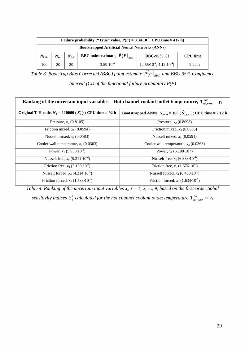