Quantitative Cost of Quality Model in Manufacturing Supply ... · Quantitative Cost of Quality...
113
Quantitative Cost of Quality Model in Manufacturing Supply Chain Ehsan Ayati Concordia Institue for Information Systems Engineering Presented in partial fulfillment of the requirement For degree of Master of Applied Science (Quality Systems Engineering) at Concordia University, Montreal, Quebec, Canada © Ehsan Ayati 2013
Transcript of Quantitative Cost of Quality Model in Manufacturing Supply ... · Quantitative Cost of Quality...

Quantitative Cost of Quality Model in
Manufacturing Supply Chain
Ehsan Ayati
Concordia Institue for Information Systems Engineering
Presented in partial fulfillment of the requirement
For degree of Master of Applied Science (Quality Systems Engineering) at
Concordia University,
Montreal, Quebec, Canada
© Ehsan Ayati 2013
CONCORDIA UNIVERSITYSchool of Graduate Studies
This is to certify that the thesis prepared
By:
Entitled:
and submitted in partial fulfillment of the requirements for the degree of
complies with the regulations of the University and meets the accepted standards withrespect to originality and quality.
Signed by the final examining committee:
______________________________________ Chair
______________________________________ Examiner
______________________________________ Examiner
______________________________________ Supervisor
Approved by ________________________________________________Chair of Department or Graduate Program Director
________________________________________________Dean of Faculty
Date ________________________________________________
Ehsan Ayati
Quantitative Cost of Quality Model in Manufacturing Supply Chain
M.A.Sc.( Quality Systems Engineering)
Dr. S. Li
Dr. K. Demirli
Dr. C. Wang
Dr. A. Schiffauerova
July 30, 2013
iii
Abstract
Quantitative Cost of Quality Model in Manufacturing Supply Chain
Ehsan Ayati
In the present business environment where quality is a key factor and customer
expectation of quality is ever-changing, measuring Cost of Quality (COQ) seems to be a
critical factor for organizations in order to keep or grow their market share. However,
until now the COQ has been measured almost exclusively only internally, i.e. within a
company, while the role of a supply chain in delivering quality product to end users has
been ignored. In this thesis we argue that all the entities within supply chain affect the
quality of a product or a service and their quality related activities should thus be
inevitably considered. Incorporating all the quality related costs of the supply chain
entities into the COQ measurement will create a powerful measure of improvement in an
organization. The objective of this research is to develop a mathematical model to
estimate COQ as key performance measurement within manufacturing supply chain
while considering quality Excellency status. Using classic PAF (Prevention-Appraisal-
Failure) model classification to develop mathematical model and its integration with
significant variables in supply chain entities are the key methodology in this work.
Perceived quality is assumed as an appropriate definition of quality in manufacturing
supply chain. Moreover, proposed model is examined against real time quality cost data
of manufacturing supply chain in two intervals, first at quality immaturity period and then
at quality maturity period. Statistical tools are used to validate the model and compare its
behavior in the two intervals. The results are then analyzed and discussed, and possible
future works are presented.

iv
Acknowledgements
Sincere appreciation is hereby extended to the following who with their help and support
this thesis has accomplished.
My supervisor Dr. Andrea Schiffauerova for her brilliant guidance and assistance in last
two years
My dear wife, Mehrnaz, for her endless love and kindness and support
My parents and sisters for their unconditional love and support
Mr. Babak Aminzadeh for his professional contribution in data collection process
Mr. Hosein Maleki (Finance PhD student at John Molson School of Business) for his
valuable contribution to data analysis chapter
v
Table of Contents List of Figures .................................................................................................................. viii
List of Tables ...................................................................................................................... x
1. Introduction ................................................................................................................. 1
2. Literature Review........................................................................................................ 3
2.1 Literature on Cost of quality ................................................................................ 3
2.1.1 Background on COQ..................................................................................... 3
2.1.2 COQ Models ................................................................................................. 5
2.1.3 Conclusion on COQ Models ....................................................................... 22
2.1.4 COQ Metrics ............................................................................................... 22
2.1.5 COQ Studies, Analysis Implementations ................................................... 23
2.2 Evaluation of COQ in Supply Chain .................................................................. 27
3. Research Methodology ............................................................................................. 29
3.1 Problem Definition ............................................................................................. 29
3.2 Research Design ................................................................................................. 30
3.3 Hypotheses ......................................................................................................... 30
4. Model Development.................................................................................................. 35
4.1 Input Variables ................................................................................................... 38
4.2 Decision Variables ............................................................................................. 38
4.3 Model parameters ............................................................................................... 38
4.3.1 Tier 1: Supplier ........................................................................................... 39
4.3.2 Tier 2: Manufacturer ................................................................................... 40
vi
4.3.3 Tier 3: Distribution ..................................................................................... 41
4.3.4 Tier 4: Retailer ............................................................................................ 41
4.3.5 Tier 5: Customer ......................................................................................... 42
4.4 Mathematical Functions ..................................................................................... 42
4.4.1 Quality level ................................................................................................ 43
4.4.2 Quality Cost Function ................................................................................. 44
4.5 Data Collection ................................................................................................... 49
4.5.1 Sample Size ................................................................................................. 51
4.5.2 Data Characteristics .................................................................................... 53
5. Data Analysis ............................................................................................................ 58
5.1 Subsamples Trend Verification .......................................................................... 58
5.2 Major Hypotheses Testing ................................................................................. 60
5.3 Model Modification............................................................................................ 81
6. Summary and Conclusions ....................................................................................... 82
6.1 Future works ....................................................................................................... 83
Bibliography ..................................................................................................................... 84
Appendices ........................................................................................................................ 90
1- Residual analysis results for Quality level and total COQ in immaturity period90
2- Residual Analysis Results for Quality level and total COQ in maturity period 91
3- Residual analysis results for prevention costs at quality immaturity period ...... 92
4- Residual analysis results for prevention costs at quality maturity period .......... 93
5- Residual analysis results for appraisal costs at quality immaturity period ........ 94
7- Residual analysis results for internal failure cost ............................................... 96
vii
8- Residual analysis results for external failure costs at immaturity period ........... 97
9- Residual analysis results for external failure costs at maturity period ............... 98
10- SAS program code ............................................................................................. 99
viii
List of Figures
Figure 2.1 Economics of quality of Conformance Juran (1951) ........................................ 8
Figure 2.2 Harrington PQC model (Harrington 1987)...................................................... 12
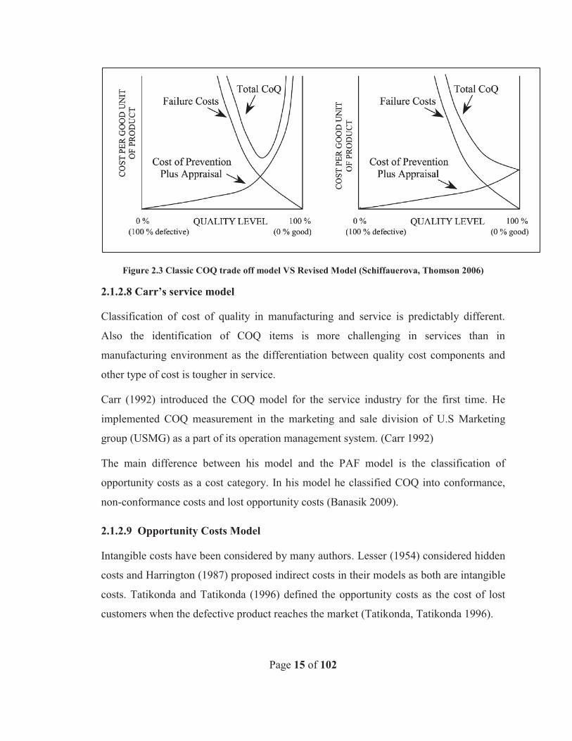
Figure 2.3 Classic COQ trade off model VS Revised Model (Schiffauerova, Thomson
2006) ................................................................................................................................. 15
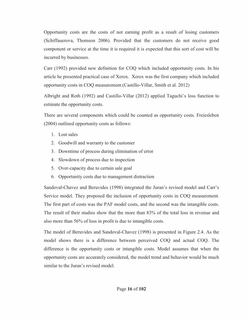
Figure 2.4 COQ considering opportunity costs (SANDOVAL-CHÁVEZ, Beruvides
1998) ................................................................................................................................. 17
Figure 2.5 COQ model integrating profit ......................................................................... 18
Figure 2.6 Ittner’s Continuous improvement COQ model (Ittner 1996) .......................... 20
Figure 2.7 Freiesleben Continuous improvement COQ model (Freiesleben 2004) ......... 21
Figure 4.1Supply Chain Network process flow chart considering COQ .......................... 37
Figure 4.2 Total COQ for whole samples ......................................................................... 55
Figure 5.1 COQ trend in the first subsample .................................................................... 59
Figure 5.2 COQ trend in second subsample Major Hypotheses Testing .......................... 60
Figure 5.3 Quality Level and COQ trend in whole samples ............................................. 61
Figure 5.4 Residual plot and fit plot for quality level and COQ regression in immaturity
period ................................................................................................................................ 62
Figure 5.5 Residual plot and fit plot for quality level and COQ regression in maturity
period ................................................................................................................................ 64
Figure 5.6 Residuals plot for independent variables in quality immaturity period .......... 66
Figure 5.7 Residual plot and fit plot of residual for prevention cost at maturity period .. 69
Figure 5.8 Residual plot of appraisal costs at immaturity period ..................................... 71
ix
Figure 5.9 Residual plot and fit plot of regression analysis for appraisal costs in maturity
period ................................................................................................................................ 73
Figure 5.10 Residual and fit plot for internal failure costs regression .............................. 75
Figure 5.11 Residual plot and fit plot in immaturity period ............................................. 78
Figure 5.12 Residual plot and fit plot in maturity period ................................................. 80
x
List of Tables
Table 2.1Global Metrics in COQ studies (Schiffauerova, Thomson 2006) ..................... 23
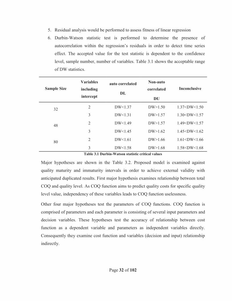
Table 3.1 Durbin-Watson statistic critical values ............................................................. 32
Table 3.2 Major Hypotheses ............................................................................................. 34
Table 4.1 Input parameters definition ............................................................................... 38
Table 4.2 Decision variables definition ............................................................................ 39
Table 4.3 Quality cost components definitions and abbreviations ................................... 45
Table 4.4 Costs components classification based on PAF model ..................................... 50
Table 4.5 Whole Sample Descriptive Statistics ................................................................ 54
Table 4.6 First Sample Descriptive Statistics ................................................................... 54
Table 4.7 Second Sample Descriptive Statistics ............................................................... 54
Table 4.8 Descriptive statistics of decision variables for whole sample .......................... 56
Table 4.9 Descriptive statistics of decision variables for first sample .............................. 56
Table 4.10 Descriptive statistics of decision variables for second sample ....................... 56
Table 5.1 Regression analysis for total quality costs and quality level in immaturity
period ................................................................................................................................ 62
Table 5.2 Regressions analysis for total quality costs and quality level in maturity period
........................................................................................................................................... 63
Table 5.3 Correlation matrix of actual good product, lead-time and prevention costs in
immaturity period.............................................................................................................. 65
Table 5.4 Multiple regressions analysis for prevention costs in immaturity period ........ 66
xi
Table 5.5 Correlation matrix of actual good product, lead-time and prevention costs in
maturity period .................................................................................................................. 67
Table 5.6 Regression analysis results for prevention costs and lead-time deviation in
maturity period .................................................................................................................. 67
Table 5.7 Regression analysis results for prevention costs and actual good product in
maturity period .................................................................................................................. 68
Table 5.8 Corroleation martix of appraisal costs .............................................................. 70
Table 5.9 Regression analysis results for appraisal costs at immaturity period ............... 70
Table 5.10 Correlation matrix of variables for appraisal costs at qualitymaturity ........... 72
Table 5.11 Regression analysis results for appraisal costs and inspection error rate at
supplier in maturity period ................................................................................................ 72
Table 5.12 Regression analysis results for appraisal costs and inspection error rate at
manufacturer in maturity period ....................................................................................... 72
Table 5.13 Regression analysis results for internal failure costs ...................................... 75
Table 5.14 Correlation matrix of variables in external failure costs in immaturity period
........................................................................................................................................... 76
Table 5.15 Multiple regression analysis of external failure costs in immaturity period ... 77
Table 5.16 Regression analysis of external failure costs with LTD in immaturity period 77
Table 5.17 Regression analysis of external failure costs with actual bad product in
immaturity period.............................................................................................................. 77
Table 5.18 Correlation matrix of variables in external failure costs in maturity period ... 79
Table 5.19 Regression analysis of external failure costs with LTD in maturity period ... 79
Table 5.20 Regression analysis of external failure costs with Actual bad product in
maturity period .................................................................................................................. 80
Page 1 of 102
1. Introduction Recent trends in global market show that today it is supply chain which competes and not
anymore a single firm. Despite all of the challenges within supply chain, like
development chain contradictions and misalignment of objectives, the emergence of
alliance and cooperation between supply chain entities play a critical role in today's
market. All tiers of supply chain from suppliers to retailers could drastically affect the
supply chain output. Thus there should be close cooperation between all entities to fortify
the chain value.
In spite of different definitions of quality from manufacturer perspective and end-user
perspective, delivering quality product is an ultimate objective of all supply chains. Cost
of quality (COQ) could be used as one of the key measures to evaluate any system
performance measurement. In the supply chain context COQ could be utilized as a key
performance measurement tool. It gives an equal opportunity to supply chain
stakeholders to examine supply chain performance in monetary terms.
There are numerous studies conducted in COQ measurement and analysis and supply
chain performance measurement, but the integration of the two is a rare case among
scholars. Some studies which study COQ in manufacturing supply chain recently
appeared. However, no comprehensive COQ model for the supply chain has been
proposed so far.
This research aims to develop a mathematical model which formulates COQ across
manufacturing supply chain. The proposed model could be utilized as a performance
measurement tool to evaluate supply chain effectiveness from quality cost point of view.
Moreover, the model is able to estimate various COQ components (prevention costs,
appraisal cost and failure costs) at different quality excellence level and their contribution
to overall COQ. Also, this research aims to study and compare proposed model at two
major COQ behaviors, first at Juran’s trade-off trend and the continuous improvement
Page 2 of 102
trend. The proposed model is modified based on the characteristics of COQ at these
behaviors.
In the second chapter of this work the comprehensive study of literature regarding COQ
has been conducted. The most popular COQ models are studied in this chapter and their
advantages and drawbacks are discussed.
In the third chapter, which is the research methodology, the problem definition, research
hypotheses and data collection procedures are described in detail.
Fourth chapter described step by step procedures to develop mathematical model and in
the fifth chapter statistical tools are used to externally validate proposed model.
Finally, the thesis is concluded in the sixth chapter, where the future works are discussed.
Page 3 of 102
2. Literature Review
2.1 Literature on Cost of quality
2.1.1 Background on COQ
Juran (1951) and Feignebaum were the first scholars who urged the necessity of
measurement of “Cost of Quality” (COQ) in quality related studies (Banasik 2009).
Feigenbaum (1956) pointed out the excessiveness of quality cost for many companies and
inevitability to measure it for the sake of business’s market position improvement.
Based on the literature in 1950s, there were several factors which lead the quality
authorities to measure quality costs. First of all, changes in the customer demands and
request for more precise and reliable product have augmented the need of cost of quality
measurement. On the other hand, the emergence of long life products, which imposed
vast amount of repair, labor, maintenance and inventory costs on the manufacturer, made
the provision of quality product more expensive than before. Furthermore, quality
authorities needed a monetary language to express and motivate senior managers to
participate in quality programs (Juran, Gryna 1993) .
Even though the formation of COQ committee in American Society of Quality (ASQ) in
1967 was the first step to the systematic and global definition and classification of COQ,
the definition of COQ has still not been agreed upon globally by the researchers and
quality involved organizations. It means that there is not a single definition which has
been accepted widely (Machowski, Dale 1998) .
Bank and Solórzano (1978) have defined the COQ as a cost incurred to keep the whole
system at the predefined quality level. Clark and Mclaughlin (1986) have divided COQ
into two types of cost. First category refers to those costs which are related to the
specifications in design and development phase and occur before delivery of product or
service. The second category involves the costs which happen after the product delivery
and are caused by the lack of conformance to the specified criteria.
Page 4 of 102
The definition of Dale and Plunkett (1995) is the definition of COQ which is generally
accepted by scholars. (Schiffauerova, Thomson 2006) have classified COQ into four
categories. First includes the cost of planning, implementation and controlling any quality
system in the organization, while the second category comprises the cost of resources
which cross-functionally are committed to maintain or reach to specified quality level.
The third category refers to the cost of quality failure, and, finally, the fourth one to the
other quality related costs.
In general COQ is assumed as a sum of amount of cost which and organization is paying
in order to achieve a good quality and amount of cost which has been incurred due to the
bad quality. The first COQ component is known as quality conformance cost and the
latter as quality nonconformance cost. (Schiffauerova, Thomson 2006).
British Standard Institution publication BS6143, (1981) developed its own definition of
COQ. In 1990 they revised their definition and published “Guide to the Economics of
Quality”. The definition is comprised of two subdivisions. First is based on the process
cost model and second is based on PAF model which will be defined later in this
literature review. It defines COQ as “cost in assuring quality as well as loss incurred
when quality is not achieved”.
Loss of consensus over cost items in COQ is the fundamental reason why ambiguity
exists in definition of COQ (Castillo-Villar, Smith et al. 2012). Dale and Plunkett (1991)
stated that there is not an agreement between accountants in what to include as a COQ.
Moreover it depends on the industry and also on the chief executive officer eagerness
towards implementation of quality programs, because quality experts are adding more
cost components or even dropping some cost components so as to signify their financial
impact (Dale, Plunkett 1999) .
Implication in definition of quality also made the definition of COQ more complicated.
Castillo- Villar, smith et al. (2012) indicated that new trends in definition of quality like
Juran definition “fitness to use” or Garvin’s new dimension of quality, not only
complicated definition of COQ but even added more intangible cost component to the
COQ.
Page 5 of 102
As a result of these inconsistencies, quality authorities, as for example ASQ, define COQ
simply based on nothing but cost components. They define COQ as a cost to prevent poor
quality in product and service and not the cost incurred to achieve high quality. Literally
they define COQ base on the COQ classification. Despite the inconsistency in the COQ
definition, Feigenbaum’s PAF classification of COQ to prevention (P), appraisal (A) and
failure (F) costs is the worldwide accepted taxonomy used to classify COQ (Castillo-
Villar, Smith et al. 2012). PAF model has gained universal acceptance amongst
researchers and organizations like ASQ. There are some other classifications of COQ
which will be discussed in the following sections.
2.1.2 COQ Models
COQ components are acquired through the COQ classification. Subsequently, the COQ
classification is implied in the COQ models. Plunkett and Dale (1988) conducted
extensive research on the COQ models. They studied several conceptual COQ models
and also generated some COQ models based on the real data from industries. They have
analyzed the relationship of COQ components and COQ behavior and concluded that,
there is no consistency in the relationship of quality cost categories and they challenged
the existence of unique COQ behavior. According to their findings, the COQ models
could be divided into 3 distinct categories. In the first group there are the models which
highlight a difference between their quality optimum point and COQ curve slope. The
second group includes models which describe quality advancement over time and pointed
out to quality milestones. Third group plotted actual quality costs obtained via industries
and over time (Plunkett, Dale 1988, Castillo-Villar, Smith et al. 2012).
Banasik (2009) outlined the findings of Plunkett and Dale (1988) findings as follow:
1. The differences between authors' quality cost items leads to the generation of
different COQ behavior and optimum COQ points.
2. Diverse COQ categories combinations proposed by different scholars and
industries prevent appropriate analysis of each cost category impact and their
interrelationships.
Page 6 of 102
3. In some models the return on the investment seems unrealistic.
4. Top managers need to have a validated model which demonstrates their current
COQ status and predicts their future changes impact. This issue caused the
generation of several diverse COQ models.
5. The logic which implies that investment in prevention and effect would have
effect on failure cost in time lags is ignored in many of the models.
Plunkett and Dale (1988) finally concluded that many proposed COQ models are
inaccurate and misleading. Moreover, they claimed uncertainties over accuracy and
validity of optimum quality levels.
First proposed classification of COQ divided modeling theories to six groups. Juran’s
model, Lesser’s model, PAF model, the economics of quality, business management of
COQ and Juran’s revised model (SANDOVAL-CHÁVEZ, Beruvides 1998).
Schiffauerova and Thomson (2006) categorized COQ to four major categories of COQ:
PAF model, opportunity cost model, process cost model and ABC model. Later on
Castillo-Villar, smith et al. (2012) classified COQ with chronological order into ten
groups: Juran’s model, Lesser’s contribution, PAF or Crosby’s model, PQC model,
accounting COQ model, process cost model, ABC approach, Juran’s revised model,
Opportunity cost model and capital budgeting model.
There are number of models and analyses which are not included in any of above
classifications. Carr (1992) introduced the COQ model for service (the previous models
were all intended for manufacturing). Ittner (1996) proposed the continuous improvement
model as an alternative to Juran’s classic model. Miller and Morris (2000) proposed the
profit consideration COQ model. And Freiesleben (2004) proposed new continuous
improvement COQ model.
The following sections provide further explanation on all of major COQ models which
seem to have dominant impact on COQ evolution.
Page 7 of 102
2.1.2.1 Juran’s model
Juran (1951) presented a conceptual - graphical COQ model. The model is later used
quite frequently by many researchers as a foundation for their newly proposed COQ
models. In his model he classified COQ into avoidable quality costs and unavoidable
quality costs. He has used the term of “gold in mine” where the gold refers to the
avoidable quality costs which just need to be identified. He described the avoidable costs
as costs which would totally disappear when there is no defect in the system.
He classified COQ into basic manufacturing costs to meet the specification, inspection
costs, quality control costs and avoidable costs. Nevertheless, later Juran (1956) declared
that the inspection costs are in fact avoidable as well.
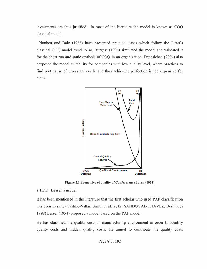
He plotted the economics of quality against quality level. His model is shown in Figure
2.1. He claimed that the total quality cost is parabolic, and concluded that losses due to
the defects will reduce exponentially as the total amount of cost spent on quality control
per product increases. And this is the point where the quality is most economical, i.e. this
is where the highest possible quality level can be reached for the lowest possible quality
costs.
He claimed that this economic optimum point for quality is not a perfection but near to it.
Based on this model, in order to achieve the complete perfection, i.e. zero defects, the
conformance cost would be infinite (Juran 1951).
Later Juran (1962) presented this model as a COQ trade-off model. The model was
designed based on the PAF, COQ classification. He emphasized on the opposite behavior
of prevention and appraisal costs on one hand, and the failure costs on the other hand.
The main objective of the model is to find the level of quality which minimizes the total
quality cost per product (Schiffauerova, Thomson 2006).
Juran (1951 and 1962) demonstrated that there is an economic point for quality where a
very high quality can be achieved for the minimum quality cost. From this point of view,
expected benefit gains from reduction of non-conformance costs would be less than the
investment in conformance activities in order to achieve higher quality level. No further
Page 8 of 102
investments are thus justified. In most of the literature the model is known as COQ
classical model.
Plunkett and Dale (1988) have presented practical cases which follow the Juran’s
classical COQ model trend. Also, Burgess (1996) simulated the model and validated it
for the short run and static analysis of COQ in an organization. Freiesleben (2004) also
proposed the model suitability for companies with low quality level, where practices to
find root cause of errors are costly and thus achieving perfection is too expensive for
them.
Figure 2.1 Economics of quality of Conformance Juran (1951)
2.1.2.2 Lesser’s model
It has been mentioned in the literature that the first scholar who used PAF classification
has been Lesser. (Castillo-Villar, Smith et al. 2012, SANDOVAL-CHÁVEZ, Beruvides
1998) Lesser (1954) proposed a model based on the PAF model.
He has classified the quality costs in manufacturing environment in order to identify
quality costs and hidden quality costs. He aimed to contribute the quality costs

Page 9 of 102
measurement as a tool to justify quality investments. In his proposal he classified quality
costs to identifiable quality costs and hidden quality costs. Scraps, reworks, customer
complaints due to defective products, inspections, testing and quality control costs were
classified as identifiable and extra costs due to poor quality, delays in production and
shipping due to defective components, business losses due to poor quality and inherited
weakness in design were classified as hidden quality costs. (Banasik 2009, Castillo-
Villar, Smith et al. 2012)
Banasik (2009) remarked his contribution to identify the impact of quality costs on
utilized resources e.g. labor, material and etc.
2.1.2.3 PAF and Crosby model
Feigenbaum (1956) presented well-known PAF model. He divided quality costs to
prevention, appraisal and failure costs. Banasik (2009) asserts that his work is the one
which shows the relationship between prevention and appraisal costs on one hand and
failure costs on the other hand. Feigenbaum (1956) described PAF components as
follows:
Prevention Costs: The costs associated with any activities to avoid poor quality
Appraisal Costs: The cost of measuring, evaluating and auditing product and service to
ensure their conformance to predefined specifications.
Internal Failure: Costs incurred due to the nonconformance of product and service to
the specification before product or service is delivered to the customer.
External Failure: Costs of nonconformance to the specification after the product or
service has been delivered to the customer
Feigenbaum (1956) illustrated the PAF model cost components interactions in the
following four steps:
1. Modern quality practice (prevention costs) leads to the decrease of failure costs
due to the reduction in number of defected components.
Page 10 of 102
2. Lower defect rate means less necessity for inspection activity and thus lower
appraisal cost.
3. Better inspection system and inspection equipment (prevention cost) also decrease
appraisal costs.
4. The new inspection and audit system will prevent defects, i.e. the reduction in
appraisal activity will lead to the reduction in defects.
Porter and Rayner (1992) concluded that the main concept of PAF model is that the
increment in prevention and appraisal costs would lead to the decrease in failure costs.
The advantage of PAF is not merely its universal acceptance among quality authorities
and researchers, but also the fact that it helps in more precise identification and
classification of quality costs (Castillo-Villar, Smith et al. 2012).
Moreover, PAF helps businesses to identify the contribution of each quality cost to total
COQ at different intervals. This enables the detection of the cost category which needs to
get more attention in order achieve higher quality level or to even reduce quality costs.
Banasik (2009) claims that the use of PAF can facilitate businesses the quality budgeting
which can be performed in accordance with their quality strategic objectives and not
simply based on historical inspection costs. Also it allows companies to determine the
return on their quality investment and to assess their investment impact on the quality.
Crosby’s (1979) classification is also in accordance with the PAF model. It categorizes
COQ to conformance and nonconformance costs. Conformance costs are defined as costs
incurred in order to obtain conformity to design specifications and to meet customer
requirements (e.g. prevention costs and appraisal costs). Nonconformance cost is the
money wasted if a defective product reaches to the customer (e.g. rework costs and
warranty costs) (Schiffauerova, Thomson 2006). Goulden and Rawlins (1995) claimed
that Crosby’s model is the same as PAF model but using different terminology.
2.1.2.4 Harrington’s Poor Quality Cost (PQC) model
Harrington (1987) introduced the PQC (Poor Quality cost) model based on the PAF
model. He asserted that PQC is aiming at the analysis of white-collar PQC and not the
Page 11 of 102
PQC in manufacturing environment. Besides, he claimed that based on the management
attitude towards quality, PQC would alerted them more than the COQ. To engage the
attention of managers and white-collars workers towards quality costs in PQC model, he
replaced the defect term with error and changed the quality target from optimum quality
cost to error free point target (Castillo-Villar, Smith et al. 2012).
He claims that his modification of the original quality costs model, will predictably lead
managers and employees towards the identification of improvement points. As a result
they will involve more in implementing and measuring continuous improvement
activities.
The concept of PQC is coming from the term “doing the things right at the first time”.
Harrington (1987) defined the PQC as “all the cost incurred to help the employee do the
job right every time and the cost of determining if the output is acceptable, plus any cost
incurred by the company and the customer because the output did not meet specification
and/or customer expectations”.
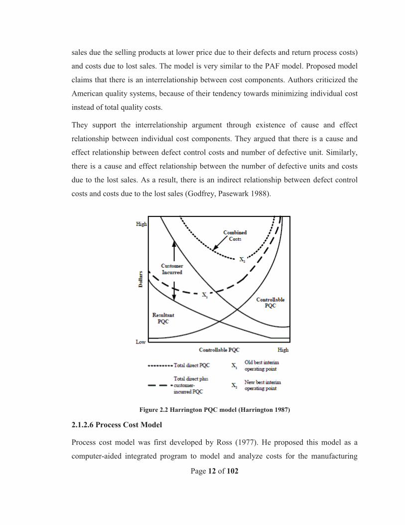
In Harington's (1987) definition the PQC are both direct and indirect PQC. The direct
PQC are controllable (prevention and appraisal), resultant (internal and external error)
and equipment related costs. Indirect costs are the costs incurred by the customer, cost of
customer dissatisfaction and loss of reputation. Although he claimed that indirect costs
are not measured in the company ledger they are part of the PQC life cycle.
Figure 2.2 demonstrates Harrington's PQC model. It shows that the increment in the
controllable costs will reduce the resultant costs and customer incurred costs.
Additionally, instead of defining an optimum quality cost point the model proposes
interim optimum operation point which dictates unavoidability of continuous
improvement.
2.1.2.5 Godfrey-Pasewark accounting COQ model
This model is proposed by (Godfrey, Pasewark 1988) and represents a COQ model from
accounting point of view. The model classified quality cost into three cost components
including defect control costs (prevention and appraisal), failure costs (rework costs, lost
Page 12 of 102
sales due the selling products at lower price due to their defects and return process costs)
and costs due to lost sales. The model is very similar to the PAF model. Proposed model
claims that there is an interrelationship between cost components. Authors criticized the
American quality systems, because of their tendency towards minimizing individual cost
instead of total quality costs.
They support the interrelationship argument through existence of cause and effect
relationship between individual cost components. They argued that there is a cause and
effect relationship between defect control costs and number of defective unit. Similarly,
there is a cause and effect relationship between the number of defective units and costs
due to the lost sales. As a result, there is an indirect relationship between defect control
costs and costs due to the lost sales (Godfrey, Pasewark 1988).
Figure 2.2 Harrington PQC model (Harrington 1987)
2.1.2.6 Process Cost Model
Process cost model was first developed by Ross (1977). He proposed this model as a
computer-aided integrated program to model and analyze costs for the manufacturing
Page 13 of 102
environment. The model seemed beneficial but not convenient to common users and
managers (Schiffauerova, Thomson 2006, Castillo-Villar, Smith et al. 2012).
Marsh (1989) used the process cost model in COQ. He used a complex method to
categorize COQ, define cost components based on the process flowchart and differentiate
quality costs components for different processes (Schiffauerova, Thomson 2006). Model
integrates conformance costs and non-conformance costs based on individual processes.
His model is very useful in businesses which implement total quality management
programs as the activities of these businesses are nothing other than interrelated
processes. Consequently, the quality costs of each process can be identified instead of
measuring a general or product based COQ. Moreover, the process cost model gives an
opportunity to evaluate current and required prevention investment action plan, i.e. to
increase or decrease the investment for each process as a prerequisite for new design
development (Marsh 1989, Porter, Rayner 1992).
Crossfield and Dale (1990) suggested a mapping method for quality assurance activities
and the related flow of information and activities in order to ease the classification of
quality costs for each process. Goulden and Rawlins (1995) utilized integrated or
functional flowchart to measure process’s quality costs.
Even though process cost model facilitates the classification and the analysis of direct
and indirect quality cost, and some scholars have highlighted its advantages over PAF, it
has not been used extensively in COQ evaluations (Goulden, Rawlins 1995).
2.1.2.7 Juran’s revised model
Juran’s (1956) trade-off model which was discussed previously suggests that there is a
quality economic point and that in order to achieve perfection the total quality cost tends
to infinity. However, this idea has been challenged by Deming (1986) afterwards. He
claimed that “Cost of selling bad quality product is too high that the best quality cost
point is where we have zero defects, thus it is not required to measure quality cost and we
have to produce zero defects”. (Deming 1986)
Page 14 of 102
Also, other researchers criticized the idea of the existence of quality cost economic point
and argued that spending on prevention activities is justifiable as long as there is a defect
in the system. (Schneiderman 1986, Plunkett, Dale 1988, Fox 1989, Porter, Rayner 1992,
Shank, Govindarajan 1994). Freiesleben (2004) also criticized classic trade-off model by
Juran. He claimed there is a problem with exponential increment of conformance costs.
He argued;
1. As quality level tends to increase, the total number of good products increases.
The conformance cost per product should thus not have incremental behavior.
2. As the sum of prevention costs increases, the sum for appraisal costs should
decrease. Similarly then, the conformance should not have incremental behavior.
Freiesleben (2004) also criticized the model because it was constructed based on the time
technological status when the quality has been poor comparing to recent progression.
Finally, he asserted that the acceptance of this model is due to “inspection mentality” of
managers.
Juran and Gryna (1993) revised the economic trade-off model. In the revised model they
claimed that perfection is achievable in finite conformance costs. They eliminated the
exponential behavior of prevention and appraisal costs. The comparison of classic and
revised Juran model is showed in Figure 2.3. However, they limited the application of
this model to the companies with high technological advancement and companies which
the clients who are very wealthy and thus businesses care much about their expenses. In
their revised model they stated that the 100% perfection is not reachable in short run and
it should be a long term goal of businesses. Freiesleben (2004) challenged the model for
not considering hidden costs. Also he claimed snap shot of perfection is not realistic as
prevention has diminishing return and return on prevention depends on already achieved
quality level, technological options and learning over time. Burgess (1996) used
simulation to validate Juran’s COQ classic and revised models. He stated that for the long
run the revised model is justifiable. Also, Ittner (1996) presented empirical study which
validated the Juran’s revised model.
Page 15 of 102
Figure 2.3 Classic COQ trade off model VS Revised Model (Schiffauerova, Thomson 2006)
2.1.2.8 Carr’s service model
Classification of cost of quality in manufacturing and service is predictably different.
Also the identification of COQ items is more challenging in services than in
manufacturing environment as the differentiation between quality cost components and
other type of cost is tougher in service.
Carr (1992) introduced the COQ model for the service industry for the first time. He
implemented COQ measurement in the marketing and sale division of U.S Marketing
group (USMG) as a part of its operation management system. (Carr 1992)
The main difference between his model and the PAF model is the classification of
opportunity costs as a cost category. In his model he classified COQ into conformance,
non-conformance costs and lost opportunity costs (Banasik 2009).
2.1.2.9 Opportunity Costs Model
Intangible costs have been considered by many authors. Lesser (1954) considered hidden
costs and Harrington (1987) proposed indirect costs in their models as both are intangible
costs. Tatikonda and Tatikonda (1996) defined the opportunity costs as the cost of lost
customers when the defective product reaches the market (Tatikonda, Tatikonda 1996).
Page 16 of 102
Opportunity costs are the costs of not earning profit as a result of losing customers
(Schiffauerova, Thomson 2006). Provided that the customers do not receive good
component or service at the time it is required it is expected that this sort of cost will be
incurred by businesses.
Carr (1992) provided new definition for COQ which included opportunity costs. In his
article he presented practical case of Xerox. Xerox was the first company which included
opportunity costs in COQ measurement.(Castillo-Villar, Smith et al. 2012)
Albright and Roth (1992) and Castillo-Villar (2012) applied Taguchi’s loss function to
estimate the opportunity costs.
There are several components which could be counted as opportunity costs. Freiesleben
(2004) outlined opportunity costs as follows:
1. Lost sales
2. Goodwill and warranty to the customer
3. Downtime of process during elimination of error
4. Slowdown of process due to inspection
5. Over-capacity due to certain sale goal
6. Opportunity costs due to management distraction
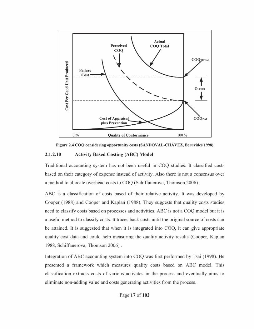
Sandoval-Chavez and Beruvides (1998) integrated the Juran’s revised model and Carr’s
Service model. They proposed the inclusion of opportunity costs in COQ measurement.
The first part of costs was the PAF model costs, and the second was the intangible costs.
The result of their studies show that the more than 83% of the total loss in revenue and
also more than 56% of loss in profit is due to intangible costs.
The model of Beruvides and Sandoval-Chavez (1998) is presented in Figure 2.4. As the
model shows there is a difference between perceived COQ and actual COQ. The
difference is the opportunity costs or intangible costs. Model assumes that when the
opportunity costs are accurately considered, the model trend and behavior would be much
similar to the Juran’s revised model.
Page 17 of 102
Figure 2.4 COQ considering opportunity costs (SANDOVAL-CHÁVEZ, Beruvides 1998)
2.1.2.10 Activity Based Costing (ABC) Model
Traditional accounting system has not been useful in COQ studies. It classified costs
based on their category of expense instead of activity. Also there is not a consensus over
a method to allocate overhead costs to COQ (Schiffauerova, Thomson 2006).
ABC is a classification of costs based of their relative activity. It was developed by
Cooper (1988) and Cooper and Kaplan (1988). They suggests that quality costs studies
need to classify costs based on processes and activities. ABC is not a COQ model but it is
a useful method to classify costs. It traces back costs until the original source of costs can
be attained. It is suggested that when it is integrated into COQ, it can give appropriate
quality cost data and could help measuring the quality activity results (Cooper, Kaplan
1988, Schiffauerova, Thomson 2006) .
Integration of ABC accounting system into COQ was first performed by Tsai (1998). He
presented a framework which measures quality costs based on ABC model. This
classification extracts costs of various activates in the process and eventually aims to
eliminate non-adding value and costs generating activities from the process.
Page 18 of 102
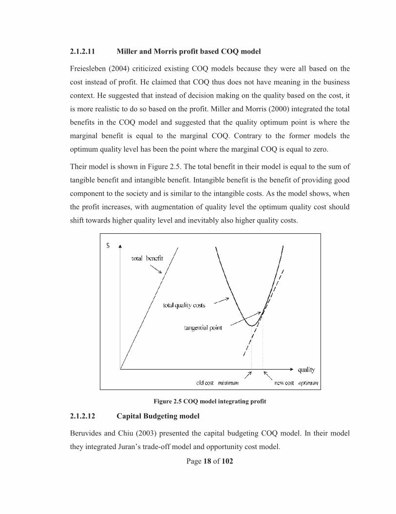
2.1.2.11 Miller and Morris profit based COQ model
Freiesleben (2004) criticized existing COQ models because they were all based on the
cost instead of profit. He claimed that COQ thus does not have meaning in the business
context. He suggested that instead of decision making on the quality based on the cost, it
is more realistic to do so based on the profit. Miller and Morris (2000) integrated the total
benefits in the COQ model and suggested that the quality optimum point is where the
marginal benefit is equal to the marginal COQ. Contrary to the former models the
optimum quality level has been the point where the marginal COQ is equal to zero.
Their model is shown in Figure 2.5. The total benefit in their model is equal to the sum of
tangible benefit and intangible benefit. Intangible benefit is the benefit of providing good
component to the society and is similar to the intangible costs. As the model shows, when
the profit increases, with augmentation of quality level the optimum quality cost should
shift towards higher quality level and inevitably also higher quality costs.
Figure 2.5 COQ model integrating profit
2.1.2.12 Capital Budgeting model
Beruvides and Chiu (2003) presented the capital budgeting COQ model. In their model
they integrated Juran’s trade-off model and opportunity cost model.
Page 19 of 102
The model suggests that the smartest decision for businesses is not to achieve 100%
conformance all the time. Their idea thus opposes the concept behind the Juran’s revised
model. They used the cost benefit analysis to study the return of investment in prevention
and appraisal activities against failure costs for specific period of the time or specific
quality program. In their model, there is a point which is named Economic Inflection
Point (EIP), which determines the point of the decision whether to cease or continue
quality programs or investment. This point varies between different industries and within
different level of quality. The model is based on the net present value objective function.
Function is comprised of three components:
1. Initial investment
2. Benefit gains through prevention and appraisal activities
3. Salvage value of investment at the end of study period
The analysis of the model of Beruvides and Chiu (2003) can be merely based on the
estimated net present value or it can be based on the comparison of internal rate of return
(IRR) against minimum attractive rate of return (MARR). Castillo-Villar, smith et al.
(2012) stated that the main objective of this model is to demonstrate balance between
return on the investment and quality level.
2.1.2.13 Continuous improvement model
Although Juran’s revised model claims that the perfection is achievable within finite
conformance costs, it does not suggest that the optimum economic quality level for all
businesses happens is at perfection. Intuitively, the cost of reaching to 100% quality level
would be inevitably too high for most of businesses. This may in fact push them out of
profit margin if they want to keep perfection (Banasik 2009).
The idea of “continuous reduction in nonconformance costs can only happen if business
invests continuously on conformance costs” has been challenged by some authors.
Schneiderman (1986) and Harrington (1987) stated that the fixed level of conformance
costs could cause continuous decrease in non-conformance costs in the continuous
improvement environment, while in the continuous improvement process, each time the
Page 20 of 102
root causes would be detected and removed without excessive investment in conformance
costs. Another model suggested the use of multi-periodic COQ model in accordance with
the organization’s stage in quality improvement process. (Noz, REDDING et al. 1989).
Fine (1986) proposed a dynamic model which emphasizes on lessons learnt. He claimed
that in his model, the lessons from former problem identification and correction would
help organization to achieve quality assurance in lower costs.
Marcellus and Dada (1991) also claimed that any investment in prevention activities
would provide learning opportunity to achieve less defective products in lower cost.
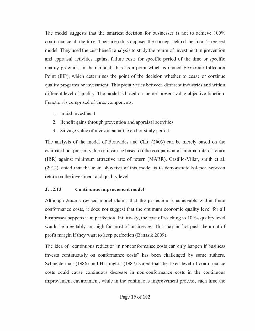
Ittner (1996) proposed the first continuous improvement COQ model against the classic
COQ model. His model suggested that due to continuous improvement policy in his COQ
model there would be point where with the same or a slightly higher spending on
conformance costs one could achieve diminishing trend in non-conformance costs. Figure
2.6 shows his proposed model.
Figure 2.6 Ittner’s Continuous improvement COQ model (Ittner 1996)
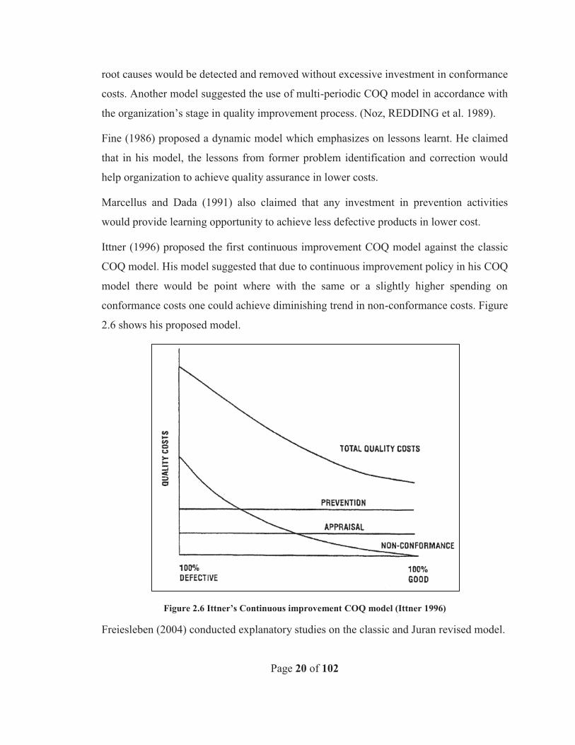
Freiesleben (2004) conducted explanatory studies on the classic and Juran revised model.
Page 21 of 102
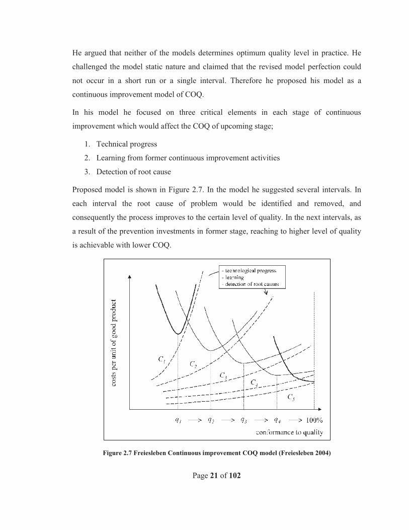
He argued that neither of the models determines optimum quality level in practice. He
challenged the model static nature and claimed that the revised model perfection could
not occur in a short run or a single interval. Therefore he proposed his model as a
continuous improvement model of COQ.
In his model he focused on three critical elements in each stage of continuous
improvement which would affect the COQ of upcoming stage;
1. Technical progress
2. Learning from former continuous improvement activities
3. Detection of root cause
Proposed model is shown in Figure 2.7. In the model he suggested several intervals. In
each interval the root cause of problem would be identified and removed, and
consequently the process improves to the certain level of quality. In the next intervals, as
a result of the prevention investments in former stage, reaching to higher level of quality
is achievable with lower COQ.
Figure 2.7 Freiesleben Continuous improvement COQ model (Freiesleben 2004)
Page 22 of 102
2.1.3 Conclusion on COQ Models
Most of the above mentioned models are conceptual and COQ model is highly dependent
on the type of COQ classification. They are not based on the accurate data, or they have
not been validated against real data. Moreover classification of quality costs will
dramatically affect the COQ behavior. Tsai and Hsu (2010) proposed a hybrid model
based on decision-making trial and evaluation (DEMATEL) method and the analytic
network process (ANP) which helps managers to choose the most relative COQ model in
accordance to their industry, quality maturity and outcome expectations.
This study of COQ models literature is a chronological illustration of COQ models
development. Some of them have been used in several studies afterwards and for some no
further studies could be found. Based on the reviewed literature it can be concluded that
despite the criticism Juran’s revised model is the most applied model due to its flexibility
and breadth.
2.1.4 COQ Metrics
Measurement of COQ does not necessarily result in quality improvement. It is a decision
support measure which helps managers to evaluate their quality investment impact and
prepare their strategic or operational quality plans. In order to be able to measure the
COQ it is required to identify COQ metrics.
There are two types of COQ metrics in the literature, detailed metrics and global metrics.
The first one measures each element of COQ and its performance individually. Cost of
resources, cost of control tools, cost of defect manufacturing per unit, cost of return items
and cost of lost customers due to poor quality are the examples of detailed metrics
(Schiffauerova, Thomson 2006).
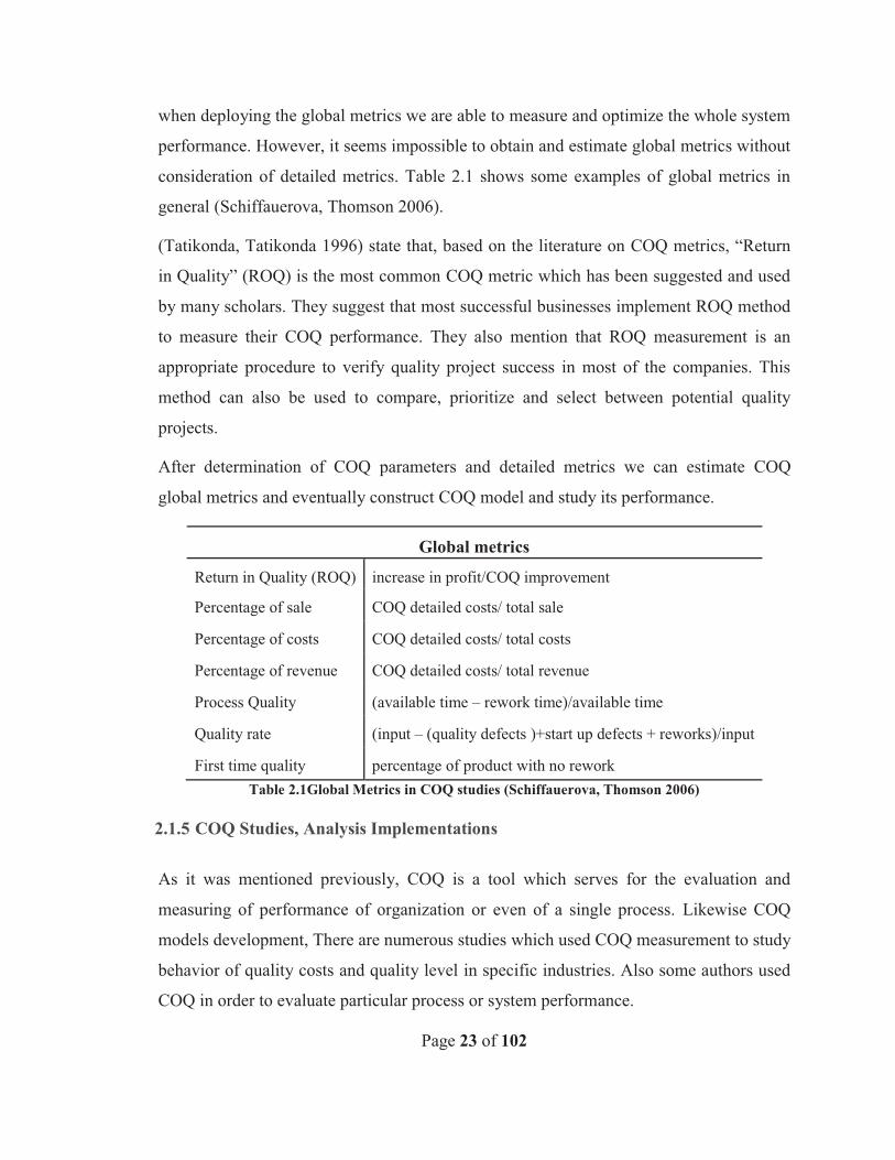
The global metrics measure global performance of system COQs. When we utilize global
metrics in COQ, we consider all of the elements of COQ and measure the contribution of
each element both individually and globally. This allows us to analyze the system
performance at various time intervals. Practically, as opposed to the detailed metrics,
Page 23 of 102
when deploying the global metrics we are able to measure and optimize the whole system
performance. However, it seems impossible to obtain and estimate global metrics without
consideration of detailed metrics. Table 2.1 shows some examples of global metrics in
general (Schiffauerova, Thomson 2006).
(Tatikonda, Tatikonda 1996) state that, based on the literature on COQ metrics, “Return
in Quality” (ROQ) is the most common COQ metric which has been suggested and used
by many scholars. They suggest that most successful businesses implement ROQ method
to measure their COQ performance. They also mention that ROQ measurement is an
appropriate procedure to verify quality project success in most of the companies. This
method can also be used to compare, prioritize and select between potential quality
projects.
After determination of COQ parameters and detailed metrics we can estimate COQ
global metrics and eventually construct COQ model and study its performance.
Global metrics
Return in Quality (ROQ) increase in profit/COQ improvement
Percentage of sale COQ detailed costs/ total sale
Percentage of costs COQ detailed costs/ total costs
Percentage of revenue COQ detailed costs/ total revenue
Process Quality (available time – rework time)/available time
Quality rate (input – (quality defects )+start up defects + reworks)/input
First time quality percentage of product with no rework Table 2.1Global Metrics in COQ studies (Schiffauerova, Thomson 2006)
2.1.5 COQ Studies, Analysis Implementations
As it was mentioned previously, COQ is a tool which serves for the evaluation and
measuring of performance of organization or even of a single process. Likewise COQ
models development, There are numerous studies which used COQ measurement to study
behavior of quality costs and quality level in specific industries. Also some authors used
COQ in order to evaluate particular process or system performance.
Page 24 of 102
(Blank, Solorzano 1978, Campanella, Corcoran 1983, Godfrey, Pasewark 1988, Ittner
1996, Sower, Quarles et al. 2007) studied the relationship of COQ as a tool for
management improvement process. They asserted that the contribution of each quality
cost category to total quality costs determines organization’s quality maturity. Al-
Tmeemy and Rahman et al (2012) conducted a qualitative research survey on the benefits
of implementation of COQ on one hand and barriers which affect implementation of
COQ between contractors on the other hand. They divided the barriers to three categories
of cultural, system and company and declared “getting management attention and
increase quality awareness” is the biggest advantage of measuring quality costs.(Al-
Tmeemy, Rahman et al. 2012)
(Gardner, Grant et al. 1995, Burgess 1996, Clark, Tannock 1999, Kiani, Shirouyehzad et
al. 2009, De Ruyter, Cardew-Hall et al. 2002, Omar, Sim et al. 2009, Omar, Murugan et
al. 2010) have used Simulation techniques to assess impact of decision variables on total
quality costs and its impact on quality improvement process.
Gardner and Grant et al. (1995) used simulation to analyze COQ model behavior in
manufacturing process. They studied the impact of defective rate, inspection and defect
removal strategy on total quality costs and eventually on quality improvement process.
They used COQ as a performance measurement tool to evaluate quality improvement
programs in two intervals. Burgess (1996) simulated system dynamic model of COQ and
proposed justification for both Juran’s traditional and revised COQ model. Clark and
Tannock (1999) used simulation to estimate the impact of different cell-manufacturing
systems and quality strategies on quality costs. De Ryter and Cardew-Hall et al. (2002)
simulated COQ in the automotive stamping plant to analyze the impact of inspection and
control error on the total quality costs. Their findings show significant effect of
inspection error on the total quality costs. Kiani and Shirouyehzad et al. (2009) utilized
system dynamics approach to model COQ. They used empirical study to validate their
model. They studied the effect of cost factor on total COQ and concluded:
Page 25 of 102
1. Prevention activity has more impact than appraisal activity on the decrease in total
COQ.
2. Prevention and appraisal activities together would have higher effect on total
COQ reduction than when they are implemented individually.
(Kiani, Shirouyehzad et al. 2009)) suggested COQ measurement to be conducted as a
long-term process within any organization regardless of its size and industry.
Omar and Sim et al. (2009) utilized simulation to assess the impact of implementation of
acceptance sampling on the incoming raw material on total COQ. Later, Omar and
Murugan et al. (2010) extended the model to assess effect of inspection error rate and
tolerance design on total COQ.
Schiffauerova and Thomson (2006) conducted a case study on measurement of COQ
within companies. They studied four companies with different types of industry and
concluded that despite the importance of COQ measurement it is not considered by many
organizations. Sower and Quarles (2007) studied the role of COQ measurement and
quality maturity on organization’s performance. In their survey above 30% of companies
measure COQ which is in accordance with former research findings. They concluded
that “the total COQ will decrease as quality improvement processes implemented but the
trend of decrease is diminishing”.
They also studied the reasons of reluctance in most organizations towards COQ
measurement. The claimed management unwillingness and lack of information system
are the major reasons of not tracking COQ in most companies.(Sower, Quarles et al.
2007)
Desai (2008) utilized COQ as a performance measurement in small and medium sizes
enterprises (SME). He emphasized on the role resource and knowledge shortage as main
reason that lead SMEs to not commit to continuous improvement. Ability to construct a
COQ budget gives an opportunity to SMEs to emphasis on failure costs in future
improvement plan and thus increasing productivity and business performance. (Desai
2008)
Page 26 of 102
Banasik (2009) conducted an extensive research on the application of COQ. He made an
elaborate comparison between COQ in manufacturing environment and water utility
plants. His finding showed that there is a big difference in all components of COQ
between manufacturing plants and water utilities. Also the percentage of total COQ in
water utilities is twice of manufacturing plants. He justified his findings with health risk
issues and regulatory reason although declaring needs for further study on the causes.
Sim and Omar et al. (2009) and Tye and Halim et al. (2011) conducted a survey
regarding implementation of COQ in Malaysian manufacturing industries. They studied
both measurement of COQ and its impact on the quality achievement in the relative
industry sector. Their findings showed high contribution of COQ measurement to non-
conformance cost reduction and organization level improvement. (Sim, Omar et al. 2009,
Tye, Halim et al. 2011)
Su Su and Shi et al (2009) studied the relationship of quality costs PAF model categories
based on the case study of automobile industry. They studied trade-off between
conformance costs and non-conformance costs by statistical analysis. Results challenged
existence of trade-off between prevention activities costs and failure costs on one hand
and appraisal activities costs and failure costs on the other hand. they estimated relative
COQ (RCOQ). Based on the results the trade-off is significant when the time lag between
conformance and non-conformance costs is considered. Outcomes underline on gradual
influence of conformance investment in failure costs reduction.
Abdul-Kader and Ganjavi et al (2010) proposed statistical quality cost model which
integrates tolerance model and investment model. The model aims to obtain optimum
cost of rework and scrap for the off-specification products. They emphasized on process
adjustment which leads to the reduction in scrap and rework, while improving the
manufacturing process and reducing quality costs. The model optimizes the cost of
process adjustment in order to avoid rejected products. They claimed that their model not
only gives managers an opportunity to estimate the optimal quality investment but even
prospect to compare the quality level and relative costs before and after the process
adjustment.
Page 27 of 102
Dror (2010) used “House of Quality” methodology to obtain and prioritize essential
prevention and appraisal activities. He used two manufacturing case studies to validate
his proposed methodology. The methodology is named the “The House of Cost of
Quality” (HCOQ). The HCOQ translates desired improvement in the language of non-
conformance costs to required effort in the language of conformance costs.
Cheah and Shahbudin et al (2011) proposed implementation of COQ as a quality
improvement program. In their study they focus on methods in identifying hidden cost of
quality and based on their case study they reveal that cutting the hidden costs would be
more useful for businesses’ profitability comparing to other routine cost cutting policies.
Liu and Li (2011) studied the relationship of reliability and COQ in coal industry in
China. They developed COQ optimization model based on the neural fuzzy network and
genetic algorithm.
2.2 Evaluation of COQ in Supply Chain
COQ reveal the implications of poor quality, quality improvement efforts and hidden
quality costs and translates them to a comprehensible language in monetary terms to all
of the system stakeholders (Castillo-Villar, Smith et al. 2012). However, COQ
measurement is mostly implemented for a specific organization or business as Srivastava
(2008) mentioned it as an in house measurement. There are numerous cases of
measurement of COQ and its implementation in organizations individually. However,
there are few studies which attempt to measure COQ in the whole supply chain networks.
Srivastava (2008) was the first author who integrated COQ in supply chain performance
measurement. The definition of COQ in supply chain based on Srivastava is:
“the sum of the costs incurred across a supply chain in preventing poor quality of product
and/or service to the final consumer, the costs incurred to ensure and evaluate that the
quality requirements are being met, and any other costs incurred as a result of poor
quality” (Srivastava 2008) P.194.
He measured COQ at selected third party manufacturing sites for a pharmaceutical
company. Ramudhin and Alzaman et al (2008) focused on integration of COQ in supply
Page 28 of 102
chain. They claimed that when COQ is incorporated in supply chain the overall operation
costs will decrease. Also they claimed that selection of supply chain network without
considering COQ is accompanied by high risk of low quality suppliers’ selection. They
studied single product three echelon supply chain and aimed to minimize total operational
costs and quality costs at the same time. They found that adding supplier quality costs to
cost objective function will lead to 16% in cost function and change the solution
considerably. Justification is because when the cost is estimated just based on the
operational costs, the supplier selection would be merely on the operational costs
regardless of their quality and COQ (Ramudhin, Alzaman et al. 2008).
Afterwards Alzaman and Bulgak et al (2009) proposed a heuristic approach to solve a
mathematical model which combines quadratic COQ function, based on the defect ratio
in all of the supply chain components. They validated their model by aerospace industry
case study.
Castillo-Villar and smith et al. (2012) developed a mathematical comprehensive model
which incorporates COQ in supply chain network. They assumed a single product three
echelon supply chain and studied the impact of defect ratio and inspection error at the
manufacturer, on total COQ and quality level. They found both Juran’s trade-off and
revised model behavior in their model in specific range of decision parameters. Later on,
Castillo-Villar and Smith et al. (2012) studied the impact of cost of quality on the supply
chain network design and solved their nonlinear model using Genetic Algorithm (GA)
and Simulated Annealing (SA).
Page 29 of 102
3. Research Methodology
3.1 Problem Definition
Based on my literature review, there are already some scholars who evaluated supply
chain network performance measurement using COQ as a key concept (Srivastava 2008,
Ramudin and Alzaman et al 2009, Castillo-Villar and smith et al 2012)
However, the former studies on performance measurement of supply chain using COQ
have concentrated on a single entity in supply chain. Srivastava (2008), Ramudin and
Alzaman et al (2009) and Castillo-Villar and smith et al (2012) focused on supply chain
performance solely form manufacturer's point of view. In other words, their studies have
considered just manufacturer performance parameters, while other supply chain entities
influential factors in measurement are ignored. As the supply chain performance
measurement aims to evaluate whole entities performance, focusing on single entity
would not have any significant advantage over in-house performance measurement. Also,
they have evaluated three echelon supply chain performance and neglected the critical
role of distribution tier in supply chain. Distributers have significant role in today’s
supply chain performance and quality as they can both affect products defect rate and
product delivery time. Thus elimination of their impact on performance does not seem
logical.
Moreover, in the previous studies the definition of quality level is limited. They confined
quality level to receiving “non-defective” measure. Voice of customer definition of
quality is totally ignored in their definition. From customer point of view, there are some
other critical factors like delivery time and availability of product which affect system
wide quality.
Finally, none of the above mentioned studies validated their models against actual costs
data. Thus their proposed models are merely conceptual and are validated internally
based on the casual relationship between their model components.
Page 30 of 102
3.2 Research Design
This research is classified as quantitative applied research. It develops a mathematical
model and validates against actual manufacturing supply chain quality costs data, and
provides COQ estimator for similar supply chains to achieve certain level of quality.
Research goal is to develop a comprehensive mathematical model in order to forecast
quality costs in four echelon manufacturing supply chain. Model utilizes COQ as a
performance measure of all of the entities within supply chain.
Consideration of customer perceived quality to define quality level is a key issue in the
model and the time series effect of quality costs and quality level is examined against
their functions parameters.
This research is basically inspired by Ramudin and Alzaman et al (2009) and Castillo-
Villar and Smith et al (2012) works. The model has been developed and then evaluated
against actual manufacturing supply chain data and is validated externally. Major
hypotheses are defined to examine model validity.
Validation is carried on by utilizing statistical linear regression analysis for all of the
quality costs components and subsequently Durbin-Watson test is used to examine the
time series effect of independent variables. Based on the statistical analysis results the
model modification and justifications would be presented.
3.3 Hypotheses
In this study, the proposed model is examined and validated against two sets of data
points, quality immaturity data and quality maturity data. Classification of data to periods
as quality maturity and immaturity periods is based on the observed COQ behavior over
time.
Before the hypotheses testing, we have to verify whether if attributed quality costs
behavior to each time interval is correct or not. It deems to examine if the first interval
COQ data follows classic trade off behavior and the second interval COQ trend is in
accordance with continuous improvement quality cost behaviors. In the first interval
conformance expenditure should be increased over time to achieve ongoing decrease in
Page 31 of 102
nonconformance costs and also existence of local economic COQ points is necessary to
be classified as trade-off model. In the second interval ongoing decrease in
nonconformance costs can be achieved by maintaining or even reducing existing
conformance costs and also non-existence of economic COQ point is crucial to categorize
the COQ behavior at this interval similar to continuous improvement model.
Evaluation of whether if the dataset follows classic trade off or continuous improvement
COQ behavior is conducted through drawing trend-line on COQ data points in both
intervals.
After the verification of distinction between COQ behaviors in two intervals the COQ
function is examined against decision parameters. In this model five major hypotheses
need to be examined in order to statistically validate proposed model. As the behavior of
COQ and quality level is studied for two datasets to verify validation results, each of
major hypotheses would have its own sub-hypotheses. Major hypotheses firstly aim to
study possible relationship between COQ function and quality level then to acknowledge
relationship between relative decision variables and parameters and cost function.
To validate proposed model set of major hypotheses is defined. Each hypothesis tests
statistical significance of the model in the following order:
1. The correlation between independent variables is tested using Pearson-coefficient
test. As the coefficient value for full dependency of variable is zero and in the real
data analysis it seems unrealistic, model’s desired value for coefficient is between
-0.5 and 0.5 for pair variables to be considered uncorrelated
2. Linear regression analysis would be conducted on all of the costs sub-functions
for each datasets
3. Values are examined against criteria. Due to the domain of study context, >
0.4 is acceptable for regression model if the homogeneity of duplicated tests is
met. This value is used to obtain the sample size and is not used to accept or reject
the hypotheses.
4. - values are examined against criteria. 95% confidence interval is predefined
criteria based on the former studies and type of industry
Page 32 of 102
5. Residual analysis would be performed to assess fitness of linear regression
6. Durbin-Watson statistic test is performed to determine the presence of
autocorrelation within the regression’s residuals in order to detect time series
effect. The accepted value for the test statistic is dependent to the confidence
level, sample number, number of variables. Table 3.1 shows the acceptable range
of DW statistics.
Sample Size Variables
including
intercept
auto correlated
DL
Non-auto
correlated
DU
Inconclusive
32 2 DW<1.37 DW>1.50 1.37<DW<1.50
3 DW<1.31 DW>1.57 1.30<DW<1.57
48 2 DW<1.49 DW>1.57 1.49<DW<1.57
3 DW<1.45 DW>1.62 1.45<DW<1.62
80 2 DW<1.61 DW>1.66 1.61<DW<1.66
3 DW<1.58 DW>1.68 1.58<DW<1.68 Table 3.1 Durbin-Watson statistic critical values
Major hypotheses are shown in the Table 3.2. Proposed model is examined against
quality maturity and immaturity intervals in order to achieve external validity with
anticipated duplicated results. First major hypothesis examines relationship between total
COQ and quality level. As COQ function aims to predict quality costs for specific quality
level value, independency of these variables leads to COQ function uselessness.
Other four major hypotheses test the parameters of COQ functions. COQ function is
comprised of parameters and each parameter is consisting of several input parameters and
decision variables. These hypotheses test the accuracy of relationship between cost
function as a dependent variable and parameters as independent variables directly.
Consequently they examine cost function and variables (decision and input) relationship
indirectly.
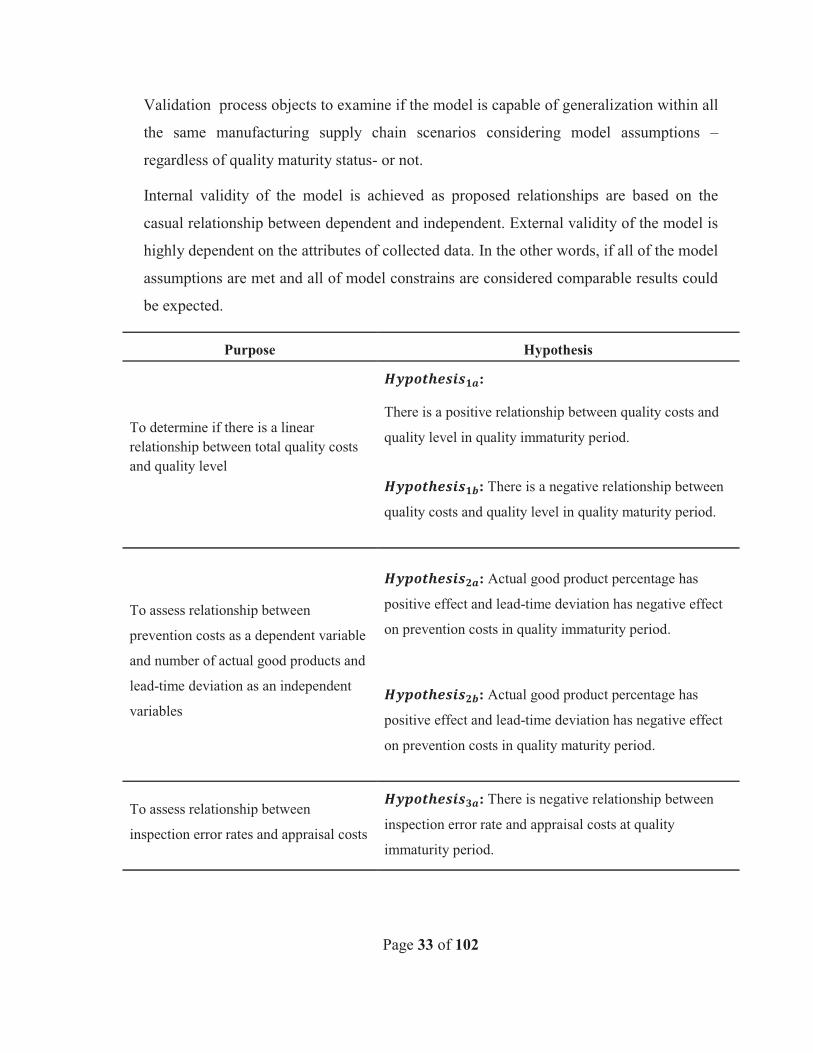
Page 33 of 102
Validation process objects to examine if the model is capable of generalization within all
the same manufacturing supply chain scenarios considering model assumptions –
regardless of quality maturity status- or not.
Internal validity of the model is achieved as proposed relationships are based on the
casual relationship between dependent and independent. External validity of the model is
highly dependent on the attributes of collected data. In the other words, if all of the model
assumptions are met and all of model constrains are considered comparable results could
be expected.
Purpose Hypothesis
To determine if there is a linear relationship between total quality costs and quality level
:
There is a positive relationship between quality costs and
quality level in quality immaturity period.
: There is a negative relationship between
quality costs and quality level in quality maturity period.
To assess relationship between
prevention costs as a dependent variable
and number of actual good products and
lead-time deviation as an independent
variables
: Actual good product percentage has
positive effect and lead-time deviation has negative effect
on prevention costs in quality immaturity period.
: Actual good product percentage has
positive effect and lead-time deviation has negative effect
on prevention costs in quality maturity period.
To assess relationship between
inspection error rates and appraisal costs
: There is negative relationship between
inspection error rate and appraisal costs at quality
immaturity period.
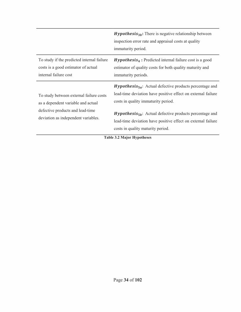
Page 34 of 102
: There is negative relationship between
inspection error rate and appraisal costs at quality
immaturity period.
To study if the predicted internal failure
costs is a good estimator of actual
internal failure cost
: Predicted internal failure cost is a good
estimator of quality costs for both quality maturity and
immaturity periods.
To study between external failure costs
as a dependent variable and actual
defective products and lead-time
deviation as independent variables.
Actual defective products percentage and
lead-time deviation have positive effect on external failure
costs in quality immaturity period.
Actual defective products percentage and
lead-time deviation have positive effect on external failure
costs in quality maturity period.
Table 3.2 Major Hypotheses

Page 35 of 102
4. Model Development As it was mentioned in literature review, former studies examined manufacturer decision
parameters impact on supply chain performance. Performance measurement system for a
supply chain should satisfy all of the supply chain entities even if their objectives are
conflicting. Measurement results has to be beneficial to all of the stakeholders within
supply chain, though this will not happen except performance measurement focuses on
individual product or process.
This Model represents a product based supply chain. It analyses quality costs as a
performance measurement for an individual product. In order to obtain more accurate
results we have constrained our model. These constraints will decrease the external
applicability of the model, but due to the inherent challenges in supply chain, e.g. conflict
of interests, development chain and large network seems inevitable. Model assumptions
are as follow:
1. Product demand is constant throughout the whole supply chain from supplier to
end-user
2. The model is suitable for the existing manufacturing firms and does not suit to
establish new supply chain.
3. There are two 100% Inspections during the whole product delivery process. First
one is when the component is delivered to the manufacturer and the other one is
when the final products are about to be shipped. Both of the inspection processes
belong to the manufacturing authorities. Sample inspections and testing during the
manufacturing process and product delivery to retailers is not considered as an
inspection process.
4. Inspection errors are error type I and error type II. Error type I is the manufacturer
risk or risk of rejecting true null hypothesis. Error type II is the customer risk and
is defined as a risk of accepting false null hypothesis. Error type I in this context
is the classification of good component as a defective one and error type II is the
classification of defective component as a good component. In this model error
Page 36 of 102
type I and II exist in supplier stage inspection, but since error type II is complex
to measure it is assumed to be equal to error type I. Error type II is the only
inspection error assumption in the manufacturing stage as the rework would be
accomplished at the same place and error type II could be highly negligible.
5. Time value of the money should be ignored to prevent the model to generate
biased results and compare the results based on quality costs only.
6. All of the scraped parts at the manufacturing stage could be sold at lower price.
7. Defective products during distribution and retailing process are recoverable, but
the cost of products return is not considered.
PAF classification of quality costs is used in this model due to its universal acceptance.
The model includes four entities in the supply chain; supplier, manufacturer, distributer
and retailer. Thus the model is four echelon supply chain. Model is based on single entity
supply chain and it is assumed that for each level of supply chain only one entity is
considered.
The model aims to estimate the total quality cost in supply chain of a specific product
while calculating each of the prevention, appraisal, internal failure and external failure
costs separately as a key performance measurement. The total COQ is nothing other than
the sum of all the cost categories.
Also, as opposed to an existing supply chain the model is not a static snapshot of supply
chain which incorporates COQ. This model dynamically represents COQ evolution in
time series. The model aims to predict total quality cost at different time intervals
considering quality level of processes. Thus appropriate definition of quality level and
quality maturity status is required in order to achieve this goal.
Model’s conceptual process flowchart map is shown in Figure 4.1. Model shows the flow
of products in the whole supply chain network form supplier to the end users. To develop
a mathematical model two types of variables and a set of parameters are defined as Input
parameters, Decision variables and Model parameters.
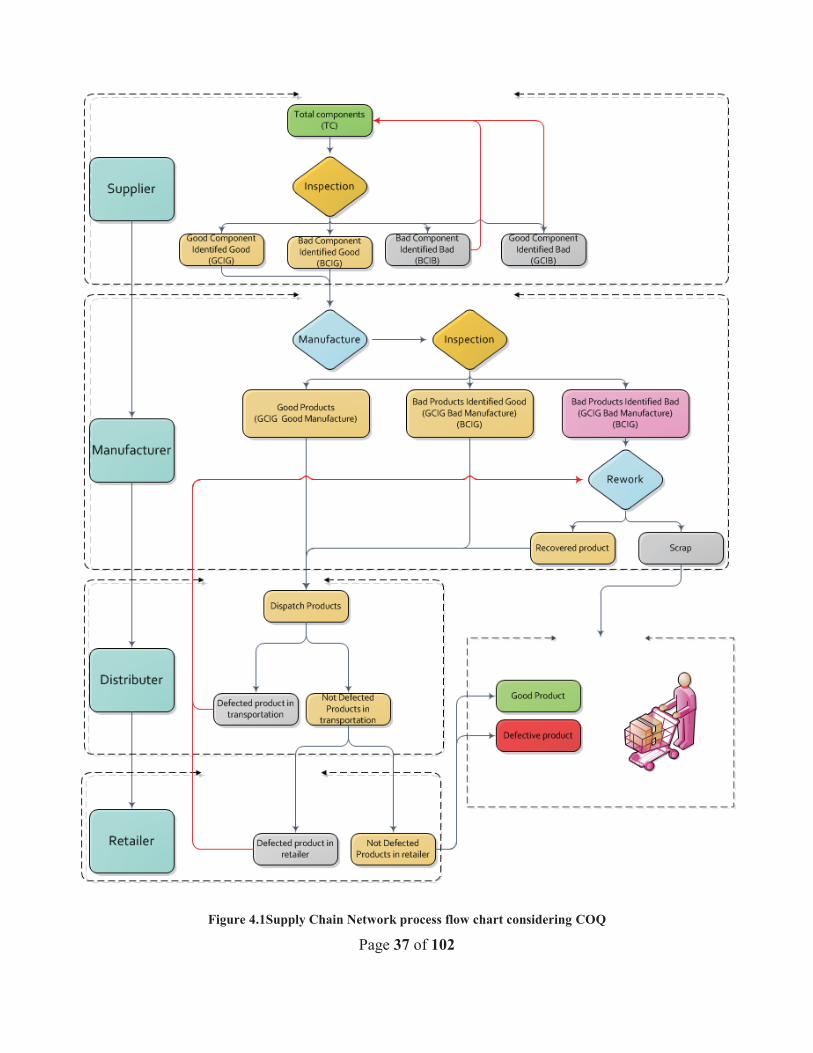
Page 37 of 102
Figure 4.1Supply Chain Network process flow chart considering COQ
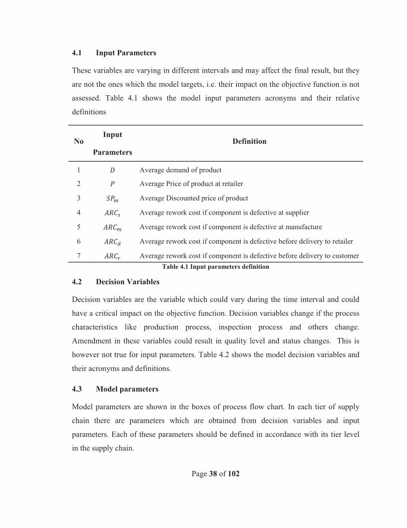
Page 38 of 102
4.1 Input Parameters
These variables are varying in different intervals and may affect the final result, but they
are not the ones which the model targets, i.e. their impact on the objective function is not
assessed. Table 4.1 shows the model input parameters acronyms and their relative
definitions
No Input
Parameters Definition
1 Average demand of product
2 Average Price of product at retailer
3 Average Discounted price of product
4 Average rework cost if component is defective at supplier
5 Average rework cost if component is defective at manufacture
6 Average rework cost if component is defective before delivery to retailer
7 Average rework cost if component is defective before delivery to customer Table 4.1 Input parameters definition
4.2 Decision Variables
Decision variables are the variable which could vary during the time interval and could
have a critical impact on the objective function. Decision variables change if the process
characteristics like production process, inspection process and others change.
Amendment in these variables could result in quality level and status changes. This is
however not true for input parameters. Table 4.2 shows the model decision variables and
their acronyms and definitions.
4.3 Model parameters
Model parameters are shown in the boxes of process flow chart. In each tier of supply
chain there are parameters which are obtained from decision variables and input
parameters. Each of these parameters should be defined in accordance with its tier level
in the supply chain.
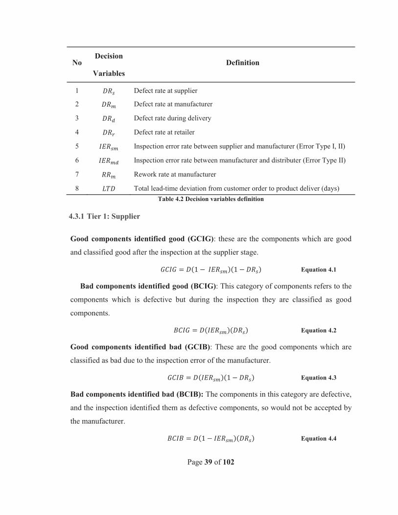
Page 39 of 102
No Decision
Variables Definition
1 Defect rate at supplier
2 Defect rate at manufacturer
3 Defect rate during delivery
4 Defect rate at retailer
5 Inspection error rate between supplier and manufacturer (Error Type I, II)
6 Inspection error rate between manufacturer and distributer (Error Type II)
7 Rework rate at manufacturer
8 Total lead-time deviation from customer order to product deliver (days) Table 4.2 Decision variables definition
4.3.1 Tier 1: Supplier
Good components identified good (GCIG): these are the components which are good
and classified good after the inspection at the supplier stage.
Equation 4.1
Bad components identified good (BCIG): This category of components refers to the
components which is defective but during the inspection they are classified as good
components.
Equation 4.2
Good components identified bad (GCIB): These are the good components which are
classified as bad due to the inspection error of the manufacturer.
Equation 4.3
Bad components identified bad (BCIB): The components in this category are defective,
and the inspection identified them as defective components, so would not be accepted by
the manufacturer.
Equation 4.4
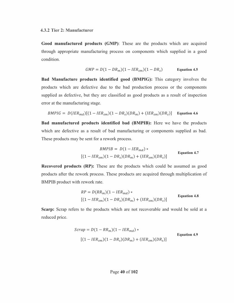
Page 40 of 102
4.3.2 Tier 2: Manufacturer
Good manufactured products (GMP): These are the products which are acquired
through appropriate manufacturing process on components which supplied in a good
condition.
Equation 4.5
Bad Manufacture products identified good (BMPIG): This category involves the
products which are defective due to the bad production process or the components
supplied as defective, but they are classified as good products as a result of inspection
error at the manufacturing stage.
Equation 4.6
Bad manufactured products identified bad (BMPIB): Here we have the products
which are defective as a result of bad manufacturing or components supplied as bad.
These products may be sent for a rework process.
Equation 4.7
Recovered products (RP): These are the products which could be assumed as good
products after the rework process. These products are acquired through multiplication of
BMPIB product with rework rate.
Equation 4.8
Scarp: Scrap refers to the products which are not recoverable and would be sold at a
reduced price.
Equation 4.9
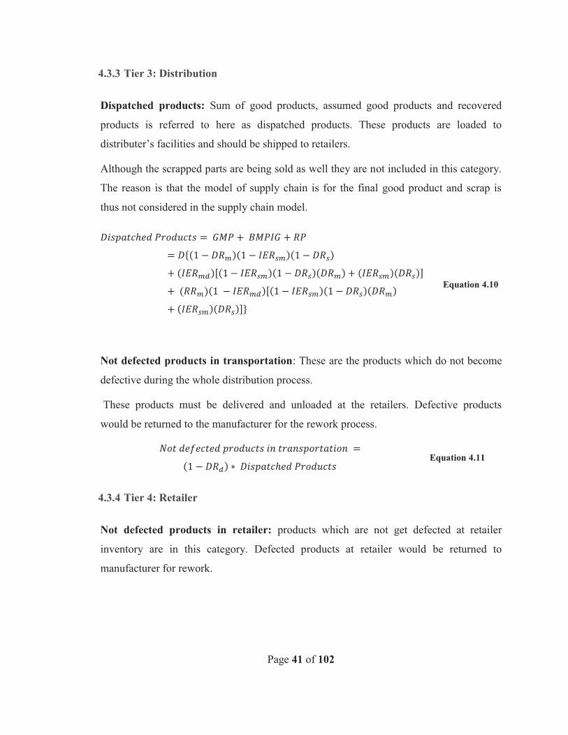
Page 41 of 102
4.3.3 Tier 3: Distribution
Dispatched products: Sum of good products, assumed good products and recovered
products is referred to here as dispatched products. These products are loaded to
distributer’s facilities and should be shipped to retailers.
Although the scrapped parts are being sold as well they are not included in this category.
The reason is that the model of supply chain is for the final good product and scrap is
thus not considered in the supply chain model.
Equation 4.10
Not defected products in transportation: These are the products which do not become
defective during the whole distribution process.
These products must be delivered and unloaded at the retailers. Defective products
would be returned to the manufacturer for the rework process.
Equation 4.11
4.3.4 Tier 4: Retailer
Not defected products in retailer: products which are not get defected at retailer
inventory are in this category. Defected products at retailer would be returned to
manufacturer for rework.
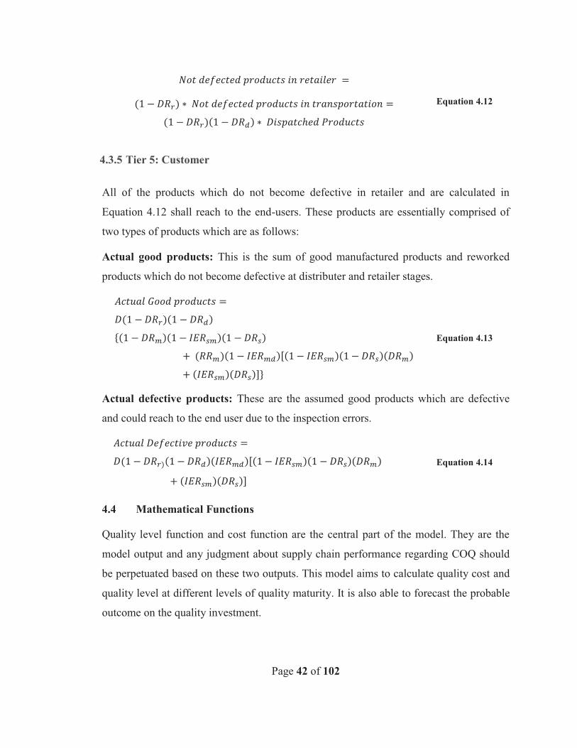
Page 42 of 102
Equation 4.12
4.3.5 Tier 5: Customer
All of the products which do not become defective in retailer and are calculated in
Equation 4.12 shall reach to the end-users. These products are essentially comprised of
two types of products which are as follows:
Actual good products: This is the sum of good manufactured products and reworked
products which do not become defective at distributer and retailer stages.
Equation 4.13
Actual defective products: These are the assumed good products which are defective
and could reach to the end user due to the inspection errors.
Equation 4.14
4.4 Mathematical Functions
Quality level function and cost function are the central part of the model. They are the
model output and any judgment about supply chain performance regarding COQ should
be perpetuated based on these two outputs. This model aims to calculate quality cost and
quality level at different levels of quality maturity. It is also able to forecast the probable
outcome on the quality investment.
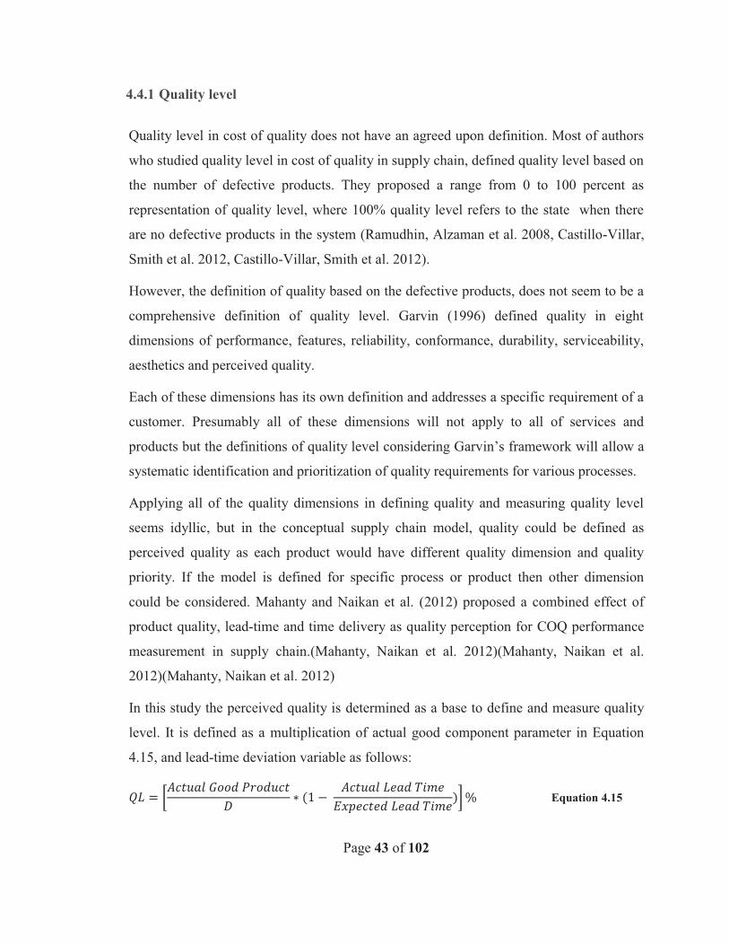
Page 43 of 102
4.4.1 Quality level
Quality level in cost of quality does not have an agreed upon definition. Most of authors
who studied quality level in cost of quality in supply chain, defined quality level based on
the number of defective products. They proposed a range from 0 to 100 percent as
representation of quality level, where 100% quality level refers to the state when there
are no defective products in the system (Ramudhin, Alzaman et al. 2008, Castillo-Villar,
Smith et al. 2012, Castillo-Villar, Smith et al. 2012).
However, the definition of quality based on the defective products, does not seem to be a
comprehensive definition of quality level. Garvin (1996) defined quality in eight
dimensions of performance, features, reliability, conformance, durability, serviceability,
aesthetics and perceived quality.
Each of these dimensions has its own definition and addresses a specific requirement of a
customer. Presumably all of these dimensions will not apply to all of services and
products but the definitions of quality level considering Garvin’s framework will allow a
systematic identification and prioritization of quality requirements for various processes.
Applying all of the quality dimensions in defining quality and measuring quality level
seems idyllic, but in the conceptual supply chain model, quality could be defined as
perceived quality as each product would have different quality dimension and quality
priority. If the model is defined for specific process or product then other dimension
could be considered. Mahanty and Naikan et al. (2012) proposed a combined effect of
product quality, lead-time and time delivery as quality perception for COQ performance
measurement in supply chain.(Mahanty, Naikan et al. 2012)(Mahanty, Naikan et al.
2012)(Mahanty, Naikan et al. 2012)
In this study the perceived quality is determined as a base to define and measure quality
level. It is defined as a multiplication of actual good component parameter in Equation
4.15, and lead-time deviation variable as follows:
Equation 4.15
Page 44 of 102
Where actual good product defined in Equation 4.13 and average expected lead-time
could be calculated from historical data.
4.4.2 Quality Cost Function
Feigenbaum’s PAF model is utilized to classify quality cost components in this model.
The quality cost is divided to four major groups: prevention costs, appraisal costs,
internal failure costs and external failure costs. In each tier of supply chain, i.e. supplier,
manufacturer, distributer and retailer, these costs will be calculated. Proposed model is
validated statistically in the upcoming chapter. Table 4.3 shows the cost components of
the model.
4.4.2.1 Prevention Costs
Prevention cost in supply chain must consider all of the prevention activities investment
in each tier of supply chain. None of the variables and parameters can define prevention
cost directly. Castillo-Villar and Smith et al (2012) claimed that the prevention cost is the
function of number of good product. They divided the prevention cost in relationship to
good product to three scenarios; supplier prevention activities, manufacturer prevention
activities and mutual prevention activities between supplier and manufacturer. They
argued that the number of good product is related to prevention activities, since as the
number of good products increases the overall quality level will increase as well and
these products do not need to be reworked.
Evidently, prevention cost is hence dependent on the number of good products which
come out of manufacturing process. Nevertheless, in our model we proposed this
relationship in terms of the good products which reach to the customer instead. The
reason is that we are considering the whole supply chain as a system beneficiary and not
just the manufacturing entity. Moreover, the definition of quality of Castillo-Villar and
Smith et al. (2012) is based on the number of good products in the whole system, which
is the reason why their analogy seems to be correct. But in our model the definition of
quality is based on the consideration of whether the product is defective and whether it
was delivered on time.
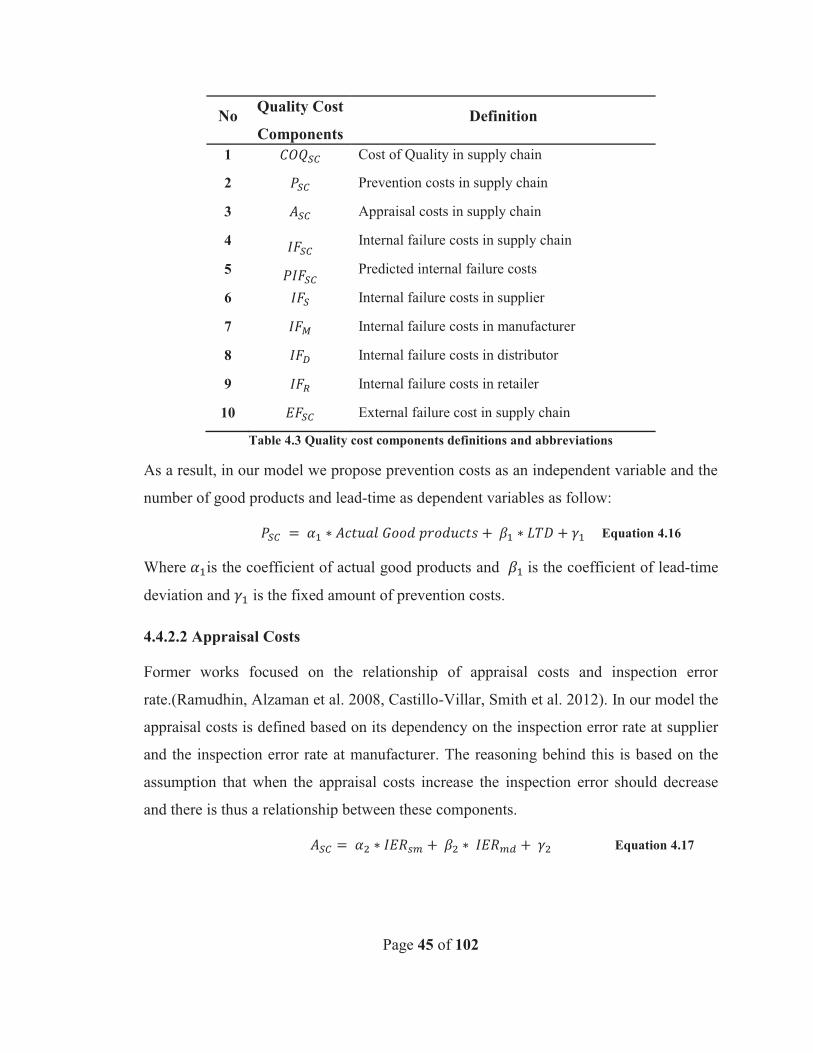
Page 45 of 102
No Quality Cost
Components Definition
1 Cost of Quality in supply chain
2 Prevention costs in supply chain
3 Appraisal costs in supply chain
4 Internal failure costs in supply chain
5 Predicted internal failure costs
6 Internal failure costs in supplier
7 Internal failure costs in manufacturer
8 Internal failure costs in distributor
9 Internal failure costs in retailer
10 External failure cost in supply chain
Table 4.3 Quality cost components definitions and abbreviations
As a result, in our model we propose prevention costs as an independent variable and the
number of good products and lead-time as dependent variables as follow:
Equation 4.16
Where is the coefficient of actual good products and is the coefficient of lead-time
deviation and is the fixed amount of prevention costs.
4.4.2.2 Appraisal Costs
Former works focused on the relationship of appraisal costs and inspection error
rate.(Ramudhin, Alzaman et al. 2008, Castillo-Villar, Smith et al. 2012). In our model the
appraisal costs is defined based on its dependency on the inspection error rate at supplier
and the inspection error rate at manufacturer. The reasoning behind this is based on the
assumption that when the appraisal costs increase the inspection error should decrease
and there is thus a relationship between these components.
Equation 4.17
Page 46 of 102
Where is the coefficient of the inspection error at the supplier stage, is the
coefficient of the inspection error at the manufacturing stage and is the fixed value
interpreted as appraisal fixed costs.
4.4.2.3 Internal Failure Costs
These are the costs incurred in the supply chain as a result of manufacturing defective
products. However, defective products are identified at inspection and test stations within
the supply chain and would not be delivered to the end-users. Internal failure costs for the
supply chain in this model are calculated based on the predicted internal failure costs.
Predicted internal failure costs are equal to the sum of the internal failure costs at each
tier of supply chain. Contrary to prevention cost and appraisal costs in the manufacturing
supply chain, the internal failure costs are calculable at each stage of supply chain
separately. They are therefore calculated based on the probable amount of defective
products at each tier of supply chain and their relative rework costs. The number of
defective products could be estimated from the defect rate at each stage, but due to the
significant variance in the rework cost of defective components the average rework costs
at each stage is used.
After estimation of predicted internal failure costs value, the actual internal failure cost is
calculable from predicted internal failure costs:
Equation 4.18
Where is the coefficient for predicted internal failure costs and is the constant value
which could be interpreted as internal failure fixed costs.
The predicted value for internal failure costs has four components which are internal
failure costs at supplier, manufacturer, distributer and retailer. The predicted internal
failure cost is comprised of 4 components shown in Equation 4.19.
Equation 4.19
: The first component of the predicted internal failure cost refers to all of the internal
failure costs incurred due to the bad component manufacturing. The defective products
are identified and classified as defective by manufacturer. Due the model inspection
Page 47 of 102
condition at supplier level, where both of the inspection error types (I and II) exist, the
good components identified bad (GCIB) in Equation 4.3 and bad components identified
bad (BCIB) in Equation 4.4 would be sent for rework. Nonetheless, as a result of supplier
self-inspection - which is considered out of the supply chain model – it is assumed that
the GCIB shall not go through rework process.
Thus the value of internal failure at supplier is equal to the multiplication of BCIB value
and average rework cost at supplier level.
Equation 4.20
: Internal failure costs at the manufacturer are in this model are comprised of two
components. The first component is similar to the internal failure costs at supplier level
and is equal to multiplication of total number of defective products to average rework
cost at manufacturing level. Total number of defective products at manufacturing stage is
equal to Bad manufactured products identified bad (BMPIB) which is shown in Equation
4.6. The second component of internal failure costs at manufacturer level is the cost of
selling irrecoverable products or scrap at discounted price, which essentially is the lost
profit instead of cost. The amount of scrap parts is shown in Equation 4.9. Also due to
large variance of product’s discounted price the average discounted price is considered in
the model. The final equation of internal failure is as follow:
Equation 4.21
: Internal failure costs at the distributer are equal to the multiplication of total number
of defective products at the delivery stage by relative average rework cost. Total number
of dispatched products to the distribution stage is shown in Equation 4.10. Multiplication
of defect rate at distributer to this value would give the total number of defective products
at this stage. The value of internal failure at distributor is shown in the following
equation:
Equation 4.22
Page 48 of 102
: Using the Equations 4.11 and 4.12 with analogy used to generate internal failure
costs at distributer tier in Equation 4.22, the internal failure costs at retailer would be as
follow:
Equation 4.23
4.4.2.4 External Failure Costs
External failure costs are the most challenging quality costs to be measured. Like
prevention costs it seems impossible to generate a function which could directly calculate
external failure costs from input parameters and decision variables. Apparently there is a
relationship between the numbers of defected products that reach to the end users and the
external failure costs. Also, based on the definition of quality in this model there could be
a relationship between external failure costs and lead-time deviation. In this model
external failure costs are assumed to be dependent variable and actual defective product
in Equation 4.14 and lead-time deviation as independent variables. The following
equation shows the external failure function:
Equation 4.24
Where is the coefficient of actual defective products, is the coefficient of lead-time
deviation and is the fixed external failure costs.
4.4.2.5 Total COQ Function
The total COQ function for supply chain is nothing but the sum of PAF components of
quality costs in the whole supply chain demonstrated in former equations. Equation 4.25
shows the COQ function.
Equation 4.25
Relative cost component functions are shown in Equations 4.16, 4.17, 4.18 and 4.24
respectively.
Page 49 of 102
4.5 Data Collection
In order to conduct external validation of the proposed model an updated manufacturing
supply chain COQ data is required. Due to the existence of overlap between COQ data
and businesses’ financial data and also because of financial data confidentiality for most
of businesses, the accurate data collection was the toughest challenge of this research.
Furthermore, the demanded data is not just confined to a single entity within supply
chain, because data should be collected from all the tiers of supply chain from suppliers
to retailers. As a consequence, the data collection process needed an extensive interaction
with supply chain entities.
Moreover, another challenge is due to the fact that the COQ data is not limited to finance
or quality departments – if they exist - but it comprises of broad spectrum of the data
from ranging from the defect rate at shop floor to quality plans investments. The
collection of such data required highly interactive cross-functional collaboration with
organizations' authorities.
Collected data for current research is from a manufacturing supply chain and by virtue of
confidential nature; name of the company must not be disclosed. Studied supply chain
product is automobile flywheel. Flywheel is used in the engine of automobile motor and
is considered as a critical engine part.
Flywheel could be manufactured via different casting processes like sand casting and die
casting or CNC machining. Focused part is manufactured through die casting and
machining processes, and the final product is delivered to a spare part retailer for sale. In
the studied manufacturing supply chain, supplier provides casted components and the
machining process is performed at the manufacturer. Both the suppliers and the
manufacturer are involved in other production processes other than flywheel, but as it
was mentioned in the literature review, supply chain performance measurement should
focus on specific product or service, and other processes are thus disregarded.
As a result this study merely focuses on the flywheel supply chain. Supply chain
considerations are centered on the manufacture entity although all of the entities are
reflected. Considerations are as follow:
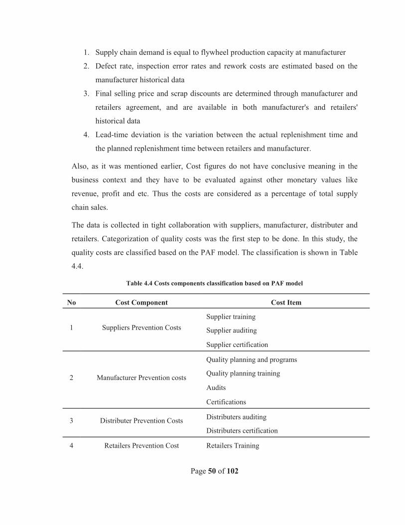
Page 50 of 102
1. Supply chain demand is equal to flywheel production capacity at manufacturer
2. Defect rate, inspection error rates and rework costs are estimated based on the
manufacturer historical data
3. Final selling price and scrap discounts are determined through manufacturer and
retailers agreement, and are available in both manufacturer's and retailers'
historical data
4. Lead-time deviation is the variation between the actual replenishment time and
the planned replenishment time between retailers and manufacturer.
Also, as it was mentioned earlier, Cost figures do not have conclusive meaning in the
business context and they have to be evaluated against other monetary values like
revenue, profit and etc. Thus the costs are considered as a percentage of total supply
chain sales.
The data is collected in tight collaboration with suppliers, manufacturer, distributer and
retailers. Categorization of quality costs was the first step to be done. In this study, the
quality costs are classified based on the PAF model. The classification is shown in Table
4.4.
Table 4.4 Costs components classification based on PAF model
No Cost Component Cost Item
1 Suppliers Prevention Costs Supplier training
Supplier auditing
Supplier certification
2 Manufacturer Prevention costs
Quality planning and programs
Quality planning training
Audits
Certifications
3 Distributer Prevention Costs Distributers auditing
Distributers certification
4 Retailers Prevention Cost Retailers Training
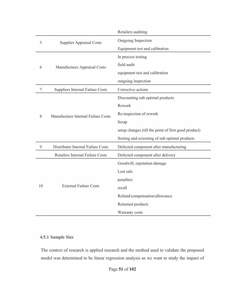
Page 51 of 102
Retailers auditing
5 Supplier Appraisal Costs Outgoing Inspection
Equipment test and calibration
6 Manufacturer Appraisal Costs
In process testing
field audit
equipment test and calibration
outgoing inspection
7 Suppliers Internal Failure Costs Corrective actions
8 Manufacturer Internal Failure Costs
Discounting sub optimal products
Rework
Re-inspection of rework
Scrap
setup changes (till the point of first good product)
Sorting and screening of sub optimal products
9 Distributer Internal Failure Costs Defected component after manufacturing
Retailers Internal Failure Costs Defected component after delivery
10 External Failure Costs
Goodwill, reputation damage
Lost sale
penalties
recall
Refund/compensation/allowance
Returned products
Warranty costs
4.5.1 Sample Size
The context of research is applied research and the method used to validate the proposed
model was determined to be linear regression analysis as we want to study the impact of
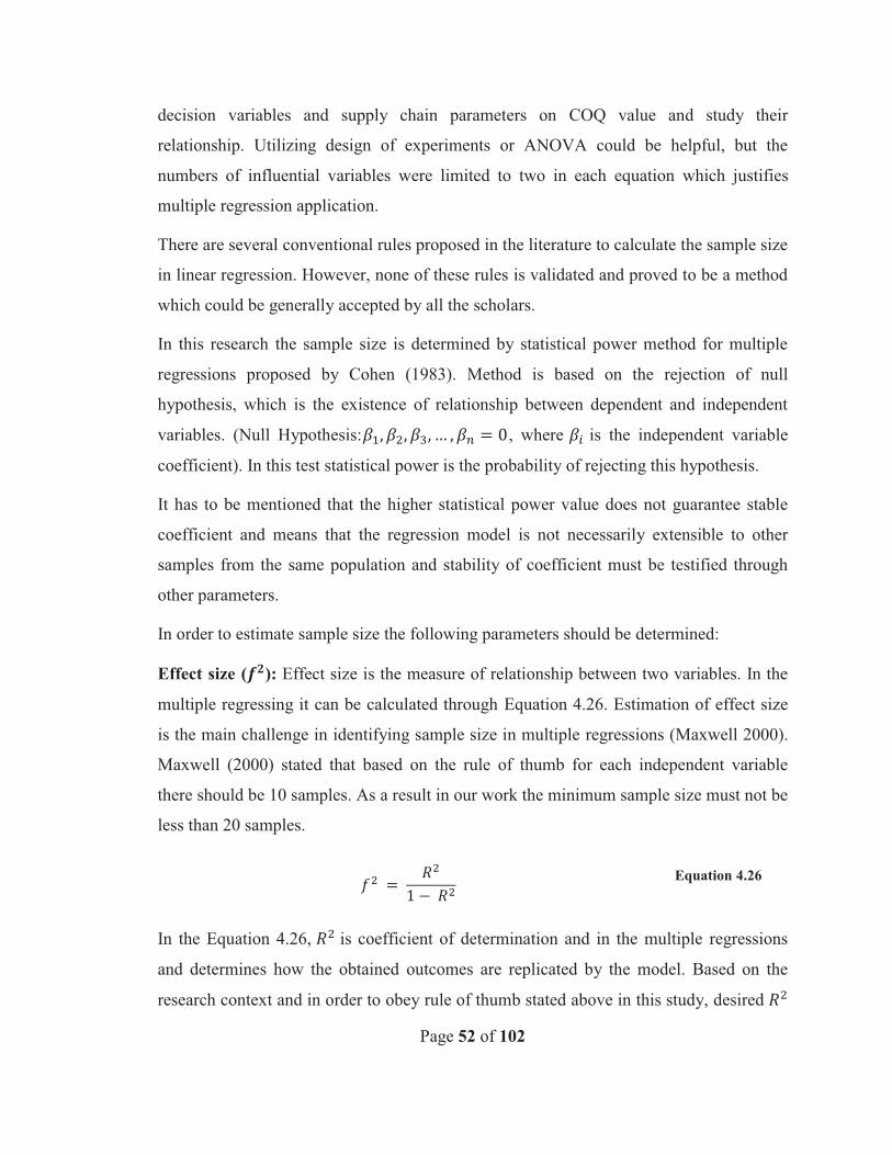
Page 52 of 102
decision variables and supply chain parameters on COQ value and study their
relationship. Utilizing design of experiments or ANOVA could be helpful, but the
numbers of influential variables were limited to two in each equation which justifies
multiple regression application.
There are several conventional rules proposed in the literature to calculate the sample size
in linear regression. However, none of these rules is validated and proved to be a method
which could be generally accepted by all the scholars.
In this research the sample size is determined by statistical power method for multiple
regressions proposed by Cohen (1983). Method is based on the rejection of null
hypothesis, which is the existence of relationship between dependent and independent
variables. (Null Hypothesis: , where is the independent variable
coefficient). In this test statistical power is the probability of rejecting this hypothesis.
It has to be mentioned that the higher statistical power value does not guarantee stable
coefficient and means that the regression model is not necessarily extensible to other
samples from the same population and stability of coefficient must be testified through
other parameters.
In order to estimate sample size the following parameters should be determined:
Effect size ( ): Effect size is the measure of relationship between two variables. In the
multiple regressing it can be calculated through Equation 4.26. Estimation of effect size
is the main challenge in identifying sample size in multiple regressions (Maxwell 2000).
Maxwell (2000) stated that based on the rule of thumb for each independent variable
there should be 10 samples. As a result in our work the minimum sample size must not be
less than 20 samples.
Equation 4.26
In the Equation 4.26, is coefficient of determination and in the multiple regressions
and determines how the obtained outcomes are replicated by the model. Based on the
research context and in order to obey rule of thumb stated above in this study, desired
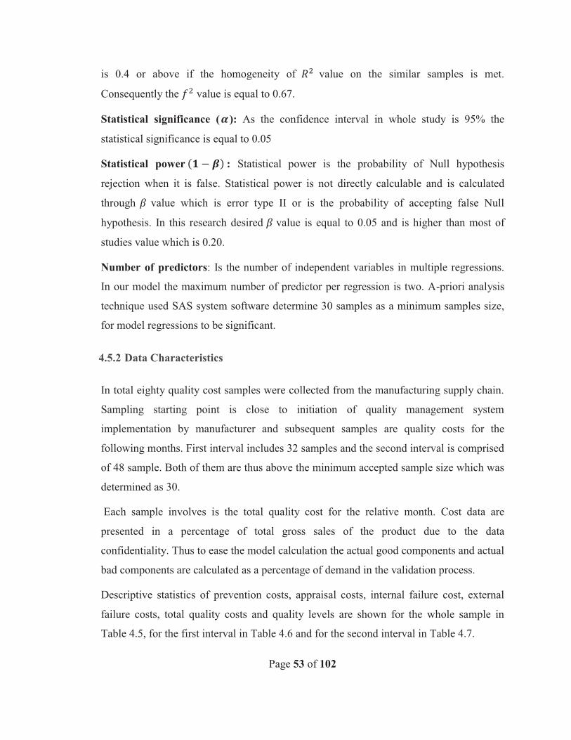
Page 53 of 102
is 0.4 or above if the homogeneity of value on the similar samples is met.
Consequently the value is equal to 0.67.
Statistical significance ( ): As the confidence interval in whole study is 95% the
statistical significance is equal to 0.05
Statistical power : Statistical power is the probability of Null hypothesis
rejection when it is false. Statistical power is not directly calculable and is calculated
through value which is error type II or is the probability of accepting false Null
hypothesis. In this research desired value is equal to 0.05 and is higher than most of
studies value which is 0.20.
Number of predictors: Is the number of independent variables in multiple regressions.
In our model the maximum number of predictor per regression is two. A-priori analysis
technique used SAS system software determine 30 samples as a minimum samples size,
for model regressions to be significant.
4.5.2 Data Characteristics
In total eighty quality cost samples were collected from the manufacturing supply chain.
Sampling starting point is close to initiation of quality management system
implementation by manufacturer and subsequent samples are quality costs for the
following months. First interval includes 32 samples and the second interval is comprised
of 48 sample. Both of them are thus above the minimum accepted sample size which was
determined as 30.
Each sample involves is the total quality cost for the relative month. Cost data are
presented in a percentage of total gross sales of the product due to the data
confidentiality. Thus to ease the model calculation the actual good components and actual
bad components are calculated as a percentage of demand in the validation process.
Descriptive statistics of prevention costs, appraisal costs, internal failure cost, external
failure costs, total quality costs and quality levels are shown for the whole sample in
Table 4.5, for the first interval in Table 4.6 and for the second interval in Table 4.7.
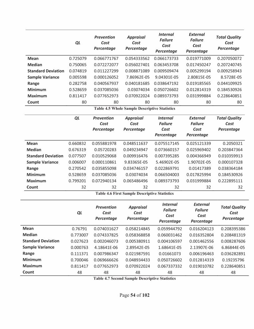
Page 54 of 102
QL Prevention
Cost Percentage
Appraisal Cost
Percentage
Internal Failure
Cost Percentage
External Failure
Cost Percentage
Total Quality Cost
Percentage
Mean 0.725079 0.066771767 0.054333562 0.066173733 0.019771009 0.207050072 Median 0.750065 0.072272077 0.056027401 0.063453708 0.017450247 0.207240745 Standard Deviation 0.074819 0.011227299 0.008871089 0.009509474 0.005299194 0.009258943 Sample Variance 0.005598 0.000126052 7.86962E-05 9.04301E-05 2.80815E-05 8.5728E-05 Range 0.282758 0.040567937 0.040181685 0.038647192 0.019185565 0.044109925 Minimum 0.528659 0.037085036 0.03074034 0.050726602 0.012814319 0.184530926 Maximum 0.811417 0.077652973 0.070922024 0.089373793 0.031999884 0.228640851 Count 80 80 80 80 80 80
Table 4.5 Whole Sample Descriptive Statistics
QL Prevention Cost
Percentage
Appraisal Cost
Percentage
Internal Failure
Cost Percentage
External Failure
Cost Percentage
Total Quality Cost
Percentage
Mean 0.660832 0.055881978 0.048511637 0.075517145 0.025121339 0.2050321 Median 0.676319 0.05720283 0.049234947 0.073660157 0.025969402 0.203847364 Standard Deviation 0.077507 0.010529068 0.009916476 0.007395285 0.004366949 0.010359913 Sample Variance 0.006007 0.000110861 9.83365E-05 5.46902E-05 1.90702E-05 0.000107328 Range 0.270542 0.035855098 0.034746157 0.022869791 0.01417389 0.038364184 Minimum 0.528659 0.037085036 0.03074034 0.066504003 0.017825994 0.184530926 Maximum 0.799201 0.072940134 0.065486496 0.089373793 0.031999884 0.222895111 Count 32 32 32 32 32 32
Table 4.6 First Sample Descriptive Statistics
QL Prevention
Cost Percentage
Appraisal Cost
Percentage
Internal Failure
Cost Percentage
External Failure
Cost Percentage
Total Quality Cost
Percentage
Mean 0.76791 0.074031627 0.058214845 0.059944792 0.016204123 0.208395386 Median 0.773007 0.074337825 0.058368858 0.060031462 0.016352804 0.208481319 Standard Deviation 0.027623 0.002046073 0.005380911 0.004106597 0.001462556 0.008287606 Sample Variance 0.000763 4.18641E-06 2.89542E-05 1.68641E-05 2.13907E-06 6.86844E-05 Range 0.111371 0.007986347 0.021987591 0.01661073 0.006196463 0.036282891 Minimum 0.700046 0.069666626 0.048934433 0.050726602 0.012814319 0.19235796 Maximum 0.811417 0.077652973 0.070922024 0.067337332 0.019010782 0.228640851 Count 48 48 48 48 48 48
Table 4.7 Second Sample Descriptive Statistics
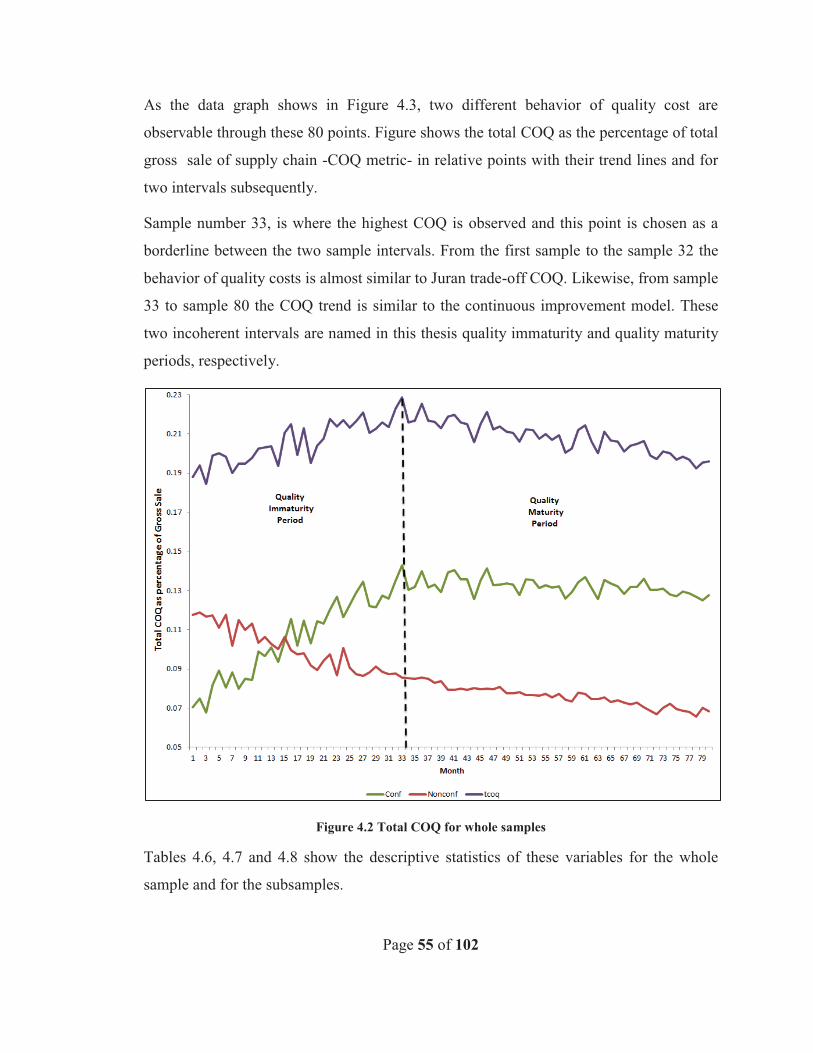
Page 55 of 102
As the data graph shows in Figure 4.3, two different behavior of quality cost are
observable through these 80 points. Figure shows the total COQ as the percentage of total
gross sale of supply chain -COQ metric- in relative points with their trend lines and for
two intervals subsequently.
Sample number 33, is where the highest COQ is observed and this point is chosen as a
borderline between the two sample intervals. From the first sample to the sample 32 the
behavior of quality costs is almost similar to Juran trade-off COQ. Likewise, from sample
33 to sample 80 the COQ trend is similar to the continuous improvement model. These
two incoherent intervals are named in this thesis quality immaturity and quality maturity
periods, respectively.
Figure 4.2 Total COQ for whole samples
Tables 4.6, 4.7 and 4.8 show the descriptive statistics of these variables for the whole
sample and for the subsamples.
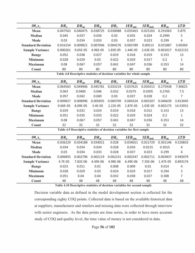
Page 56 of 102
DR_s_ Mean 0.047563 0.040475 0.038725 0.030088 0.035463 0.025163 0.291063 5.875
Median 0.045 0.037 0.036 0.03 0.035 0.024 0.2995 5 Mode 0.03 0.034 0.033 0.03 0.037 0.023 0.299 4
Standard Deviation 0.016154 0.009821 0.007046 0.004276 0.003789 0.00513 0.031887 3.00369 Sample Variance 0.000261 9.65E-05 4.96E-05 1.83E-05 1.44E-05 2.63E-05 0.001017 9.022152
Range 0.052 0.038 0.027 0.019 0.018 0.019 0.153 13 Minimum 0.028 0.029 0.03 0.022 0.029 0.017 0.2 1 Maximum 0.08 0.067 0.057 0.041 0.047 0.036 0.353 14
Count 80 80 80 80 80 80 80 80 Table 4.8 Descriptive statistics of decision variables for whole sample
DR_s_ Mean 0.064563 0.049906 0.045781 0.033219 0.037625 0.030313 0.275938 7.90625
Median 0.063 0.0485 0.046 0.032 0.0375 0.0305 0.2765 7.5 Mode 0.057 0.042 0.049 0.03 0.037 0.028 0.2 7
Standard Deviation 0.009827 0.008996 0.005835 0.004709 0.004324 0.003207 0.046639 3.813045 Sample Variance 9.66E-05 8.09E-05 3.4E-05 2.22E-05 1.87E-05 1.03E-05 0.002175 14.53931
Range 0.029 0.032 0.024 0.019 0.018 0.012 0.153 13 Minimum 0.051 0.035 0.033 0.022 0.029 0.024 0.2 1 Maximum 0.08 0.067 0.057 0.041 0.047 0.036 0.353 14
Count 32 32 32 32 32 32 32 32 Table 4.9 Descriptive statistics of decision variables for first sample
DR_s_ Mean 0.036229 0.034188 0.034021 0.028 0.034021 0.021729 0.301146 4.520833
Median 0.034 0.034 0.034 0.028 0.034 0.0215 0.3015 4 Mode 0.03 0.034 0.033 0.028 0.037 0.023 0.299 4
Standard Deviation 0.006855 0.002796 0.002119 0.002231 0.002547 0.002711 0.003837 0.945079 Sample Variance 4.7E-05 7.82E-06 4.49E-06 4.98E-06 6.49E-06 7.35E-06 1.47E-05 0.893174
Range 0.023 0.011 0.01 0.008 0.009 0.01 0.014 4 Minimum 0.028 0.029 0.03 0.024 0.029 0.017 0.294 3 Maximum 0.051 0.04 0.04 0.032 0.038 0.027 0.308 7
Count 48 48 48 48 48 48 48 48 Table 4.10 Descriptive statistics of decision variables for second sample
Decision variable data as defined in the model development section is collected for the
corresponding eighty COQ points. Collected data is based on the available historical data
at suppliers, manufacturer and retailers and missing data were collected through interview
with senior engineers. As the data points are time series, in order to have more accurate
study of COQ and quality level, the time value of money is not considered in data.
Page 57 of 102
Furthermore, input parameters are cost values which vary drastically and are dependent
on several internal and external factors which identified at tactical and strategic levels
like market demand, production practices and etc. In this study, their evaluation is based
on the average estimation of field managers as there were not sufficient historical
accurate recorded data for them for the whole study period. Several interviews have been
conducted with field engineers, production supervisors and senior managers at
manufacturer and supplier and they played an interactive role in whole data collection
and data analysis. Also in some cases field tests have been conducted to examine the
conformity of obtained data. These values are assumed to be constant throughout the
sampling period. Tables 4.6, 4.7 and 4.8 show the descriptive statistics of these variables
for the whole sample and for the subsamples.
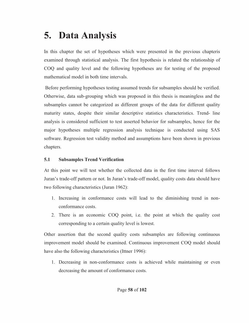
Page 58 of 102
5. Data Analysis In this chapter the set of hypotheses which were presented in the previous chapteris
examined through statistical analysis. The first hypothesis is related the relationship of
COQ and quality level and the following hypotheses are for testing of the proposed
mathematical model in both time intervals.
Before performing hypotheses testing assumed trends for subsamples should be verified.
Otherwise, data sub-grouping which was proposed in this thesis is meaningless and the
subsamples cannot be categorized as different groups of the data for different quality
maturity states, despite their similar descriptive statistics characteristics. Trend- line
analysis is considered sufficient to test asserted behavior for subsamples, hence for the
major hypotheses multiple regression analysis technique is conducted using SAS
software. Regression test validity method and assumptions have been shown in previous
chapters.
5.1 Subsamples Trend Verification
At this point we will test whether the collected data in the first time interval follows
Juran’s trade-off pattern or not. In Juran’s trade-off model, quality costs data should have
two following characteristics (Juran 1962):
1. Increasing in conformance costs will lead to the diminishing trend in non-
conformance costs.
2. There is an economic COQ point, i.e. the point at which the quality cost
corresponding to a certain quality level is lowest.
Other assertion that the second quality costs subsamples are following continuous
improvement model should be examined. Continuous improvement COQ model should
have also the following characteristics (Ittner 1996):
1. Decreasing in non-conformance costs is achieved while maintaining or even
decreasing the amount of conformance costs.
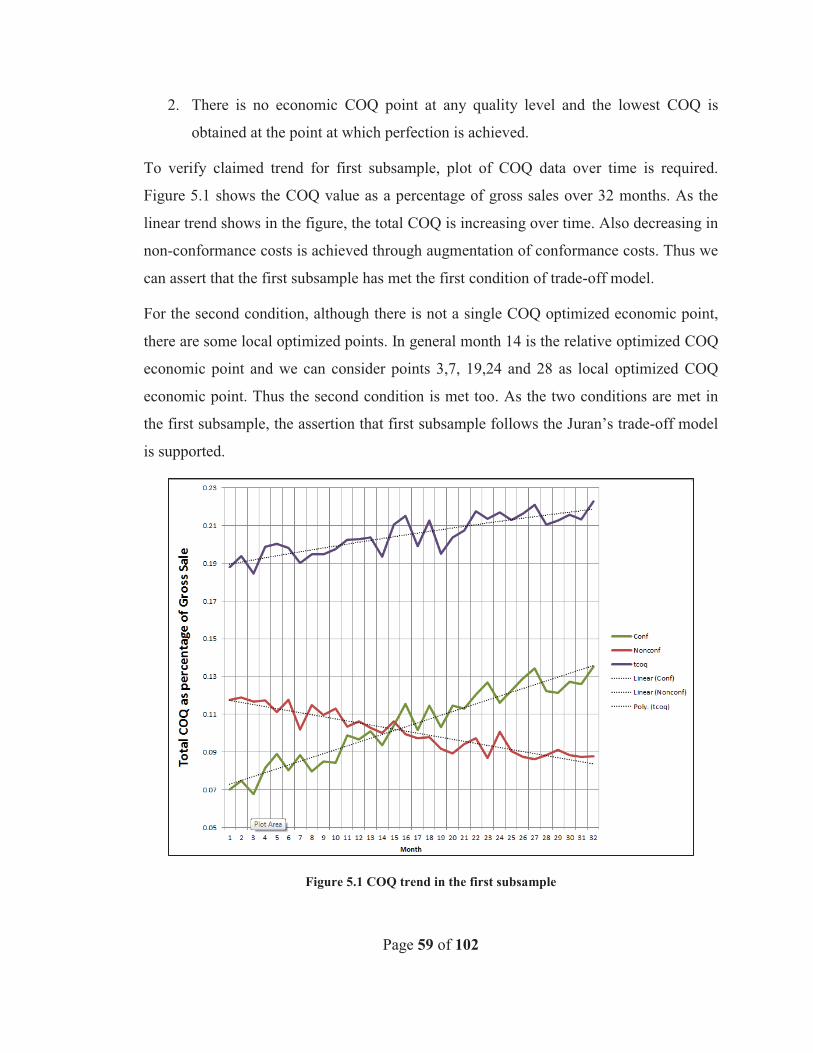
Page 59 of 102
2. There is no economic COQ point at any quality level and the lowest COQ is
obtained at the point at which perfection is achieved.
To verify claimed trend for first subsample, plot of COQ data over time is required.
Figure 5.1 shows the COQ value as a percentage of gross sales over 32 months. As the
linear trend shows in the figure, the total COQ is increasing over time. Also decreasing in
non-conformance costs is achieved through augmentation of conformance costs. Thus we
can assert that the first subsample has met the first condition of trade-off model.
For the second condition, although there is not a single COQ optimized economic point,
there are some local optimized points. In general month 14 is the relative optimized COQ
economic point and we can consider points 3,7, 19,24 and 28 as local optimized COQ
economic point. Thus the second condition is met too. As the two conditions are met in
the first subsample, the assertion that first subsample follows the Juran’s trade-off model
is supported.
Figure 5.1 COQ trend in the first subsample

Page 60 of 102
For the second subsample also the two conditions of continuous improvement trend
should be satisfied. As the trend shows in Figure 5.2, the total quality costs are constantly
decreasing hence the non-conformance costs are decreasing too. This could be justified as
a result of continuous improvement nature where the effect of root problem solving effect
in former stages and advancement in knowledge and processes leads to achieve lower
non-conformance costs while maintaining same or lower investment in conformance
costs. As a result we can say that the first condition is met.
Also based on the CoQ graph trend in Figure 5.2, there is no optimized or even local
optimized COQ economic point in collected data in second subsample, subsequently the
second condition is met too. Finally, based on our trend lines in second subsample, the
corresponding COQ trend could be considered as continuous improvement COQ model.
Figure 5.2 COQ trend in second subsample Major Hypotheses Testing
5.2 Major Hypotheses Testing
As it was mentioned previously, linear regression analysis is utilized to examine the
proposed hypotheses. Within the major hypotheses, the fifth hypothesis, similarly as the

Page 61 of 102
four explanatory hypotheses, is a prerequisite for data subgrouping. It examines the effect
of COQ on quality level and their significant relationship in two subsamples. This
hypothesis is constructed based on explanatory hypotheses results which acknowledged
presence of different COQ behaviors. Test is required to be conducted in order to signify
the subgrouping through examination of relationship between COQ and quality level in
different quality maturity status.
Hypotheses 1 to 5 statistically test model components. Using simple or multiple
regression analysis, residual analysis and Durbin-Watson test are the steps in these
hypotheses testing.
:
There is a positive relationship between quality costs and quality level in quality
immaturity period.
There is not a positive relationship between quality costs and quality level in quality
immaturity period.
Figure 5.3 Quality Level and COQ trend in whole samples
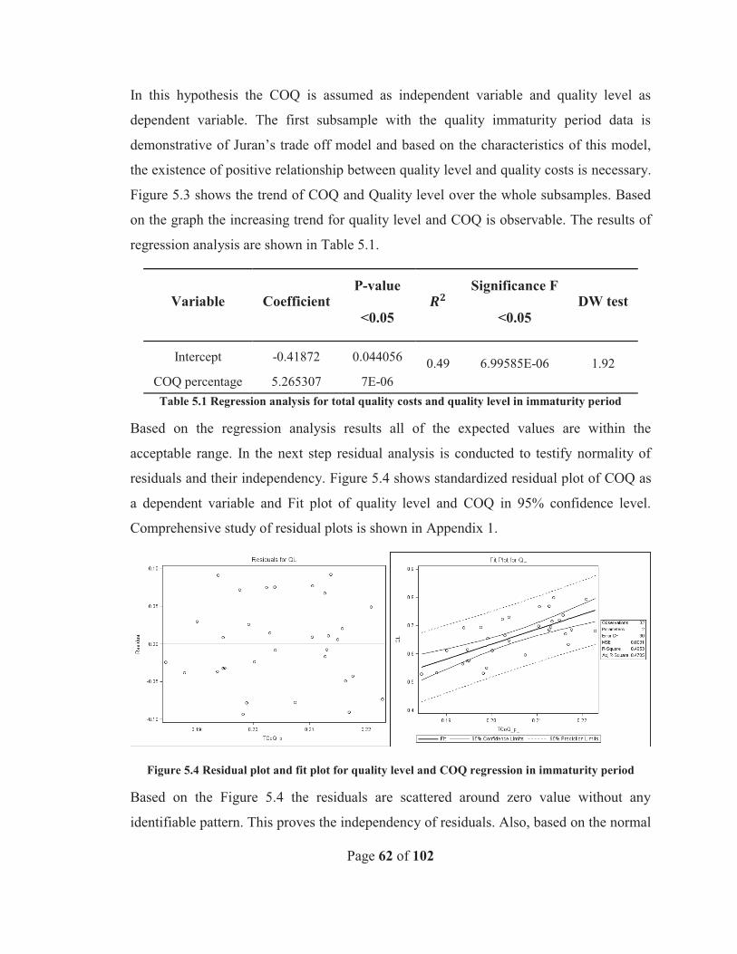
Page 62 of 102
In this hypothesis the COQ is assumed as independent variable and quality level as
dependent variable. The first subsample with the quality immaturity period data is
demonstrative of Juran’s trade off model and based on the characteristics of this model,
the existence of positive relationship between quality level and quality costs is necessary.
Figure 5.3 shows the trend of COQ and Quality level over the whole subsamples. Based
on the graph the increasing trend for quality level and COQ is observable. The results of
regression analysis are shown in Table 5.1.
Variable Coefficient P-value
<0.05
Significance F
<0.05 DW test
Intercept -0.41872 0.044056 0.49 6.99585E-06 1.92 COQ percentage 5.265307 7E-06 Table 5.1 Regression analysis for total quality costs and quality level in immaturity period
Based on the regression analysis results all of the expected values are within the
acceptable range. In the next step residual analysis is conducted to testify normality of
residuals and their independency. Figure 5.4 shows standardized residual plot of COQ as
a dependent variable and Fit plot of quality level and COQ in 95% confidence level.
Comprehensive study of residual plots is shown in Appendix 1.
Figure 5.4 Residual plot and fit plot for quality level and COQ regression in immaturity period
Based on the Figure 5.4 the residuals are scattered around zero value without any
identifiable pattern. This proves the independency of residuals. Also, based on the normal
Page 63 of 102
probability plot of residuals in Appendix 1, residuals are quite normal. As result of the
regression and the positive value of the independent variable, and also the residual
analysis, it could be concluded that we cannot reject null hypothesis and there is not
sufficient evidence to support the alternative hypothesis.
:
: There is a negative relationship between quality costs and quality level in quality
maturity period.
There is not a negative relationship between quality costs and quality level in quality
maturity period.
Similarly as in the previous hypothesis the independent variable is COQ and the
dependent variable is quality level. As the COQ data in maturity period asserted to follow
continuous improvement COQ model, there should be a negative correlation between
COQ and quality level. As it is shown in Figure 5.3, the trend of COQ in the maturity
period is decreasing while quality level is diminishing. Statistical analysis of data using
regressions is conducted and the results are shown in table 5.2.
Variable Coefficient P-value
<0.05
Significance F
<0.05 DW test
Intercept 1.303763 2.55E-24 0.59 1.39E-10 1.38 COQ percentage -2.57133 1.39E-10
Table 5.2 Regressions analysis for total quality costs and quality level in maturity period
Obtained statistics are within the acceptable range except the Durbin-Watson test
statistic. The value of DW is 1.38 which based on the DW statistic critical value table
presented in methodology chapter is within inconclusive range. It means that we cannot
claim existence or absence of autocorrelation in samples. Although test statistic is still
acceptable as there is not proven autocorrelation within sample, but existence of
autocorrelation in this hypothesis is not necessarily unpredictable, as the time is a key
factor which affects COQ and quality level. It means that the time series effect is
inevitable in this regression model and would not affect results conclusion.
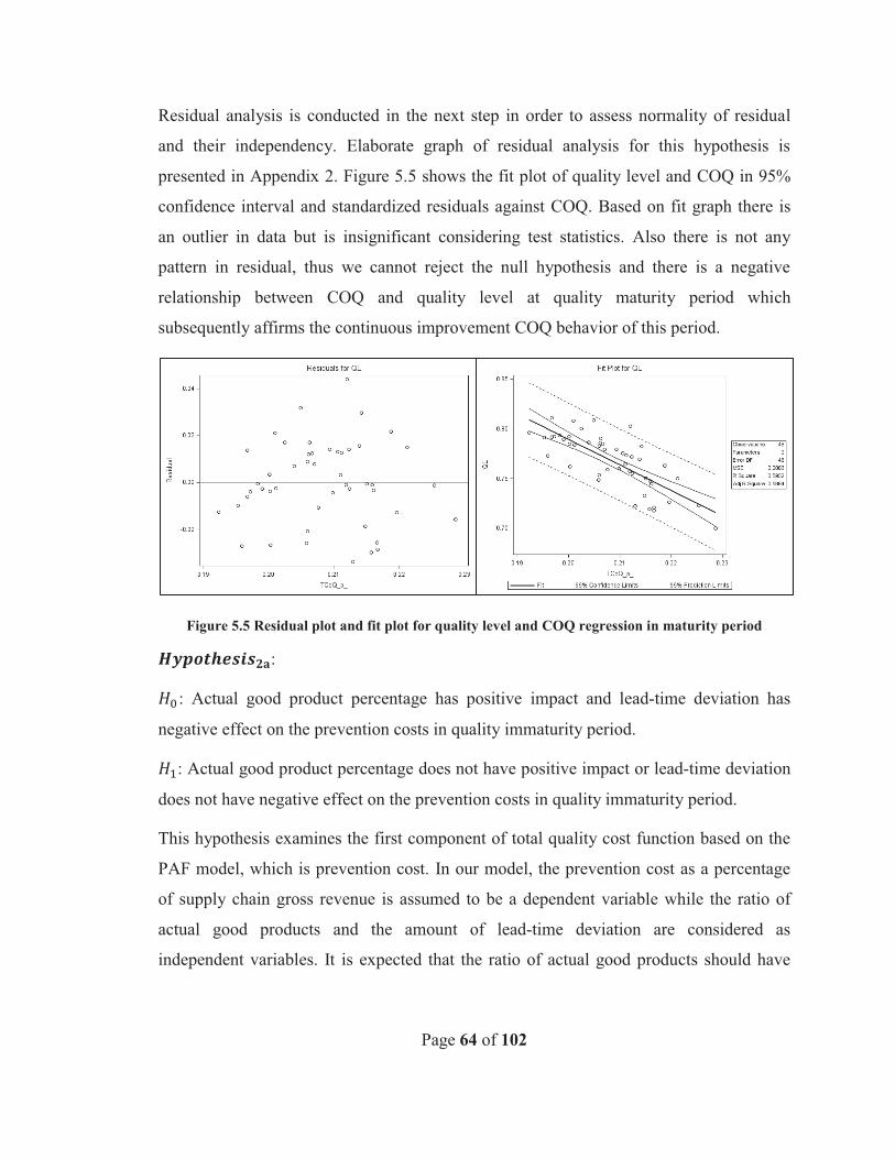
Page 64 of 102
Residual analysis is conducted in the next step in order to assess normality of residual
and their independency. Elaborate graph of residual analysis for this hypothesis is
presented in Appendix 2. Figure 5.5 shows the fit plot of quality level and COQ in 95%
confidence interval and standardized residuals against COQ. Based on fit graph there is
an outlier in data but is insignificant considering test statistics. Also there is not any
pattern in residual, thus we cannot reject the null hypothesis and there is a negative
relationship between COQ and quality level at quality maturity period which
subsequently affirms the continuous improvement COQ behavior of this period.
Figure 5.5 Residual plot and fit plot for quality level and COQ regression in maturity period
:
: Actual good product percentage has positive impact and lead-time deviation has
negative effect on the prevention costs in quality immaturity period.
: Actual good product percentage does not have positive impact or lead-time deviation
does not have negative effect on the prevention costs in quality immaturity period.
This hypothesis examines the first component of total quality cost function based on the
PAF model, which is prevention cost. In our model, the prevention cost as a percentage
of supply chain gross revenue is assumed to be a dependent variable while the ratio of
actual good products and the amount of lead-time deviation are considered as
independent variables. It is expected that the ratio of actual good products should have
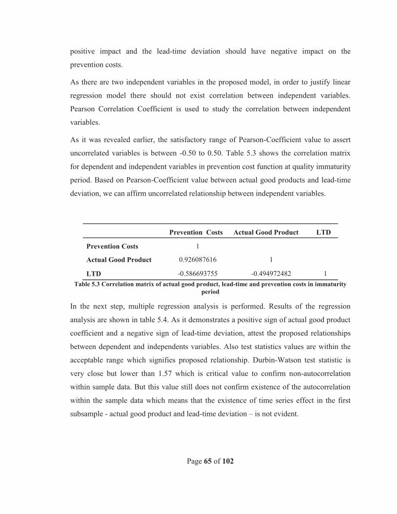
Page 65 of 102
positive impact and the lead-time deviation should have negative impact on the
prevention costs.
As there are two independent variables in the proposed model, in order to justify linear
regression model there should not exist correlation between independent variables.
Pearson Correlation Coefficient is used to study the correlation between independent
variables.
As it was revealed earlier, the satisfactory range of Pearson-Coefficient value to assert
uncorrelated variables is between -0.50 to 0.50. Table 5.3 shows the correlation matrix
for dependent and independent variables in prevention cost function at quality immaturity
period. Based on Pearson-Coefficient value between actual good products and lead-time
deviation, we can affirm uncorrelated relationship between independent variables.
Prevention Costs Actual Good Product LTD
Prevention Costs 1
Actual Good Product 0.926087616 1
LTD -0.586693755 -0.494972482 1 Table 5.3 Correlation matrix of actual good product, lead-time and prevention costs in immaturity
period
In the next step, multiple regression analysis is performed. Results of the regression
analysis are shown in table 5.4. As it demonstrates a positive sign of actual good product
coefficient and a negative sign of lead-time deviation, attest the proposed relationships
between dependent and independents variables. Also test statistics values are within the
acceptable range which signifies proposed relationship. Durbin-Watson test statistic is
very close but lower than 1.57 which is critical value to confirm non-autocorrelation
within sample data. But this value still does not confirm existence of the autocorrelation
within the sample data which means that the existence of time series effect in the first
subsample - actual good product and lead-time deviation – is not evident.
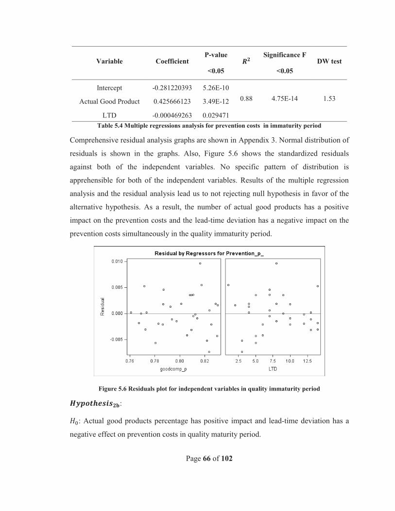
Page 66 of 102
Variable Coefficient P-value
<0.05
Significance F
<0.05 DW test
Intercept -0.281220393 5.26E-10 0.88 4.75E-14 1.53 Actual Good Product 0.425666123 3.49E-12
LTD -0.000469263 0.029471 Table 5.4 Multiple regressions analysis for prevention costs in immaturity period
Comprehensive residual analysis graphs are shown in Appendix 3. Normal distribution of
residuals is shown in the graphs. Also, Figure 5.6 shows the standardized residuals
against both of the independent variables. No specific pattern of distribution is
apprehensible for both of the independent variables. Results of the multiple regression
analysis and the residual analysis lead us to not rejecting null hypothesis in favor of the
alternative hypothesis. As a result, the number of actual good products has a positive
impact on the prevention costs and the lead-time deviation has a negative impact on the
prevention costs simultaneously in the quality immaturity period.
Figure 5.6 Residuals plot for independent variables in quality immaturity period
:
: Actual good products percentage has positive impact and lead-time deviation has a
negative effect on prevention costs in quality maturity period.
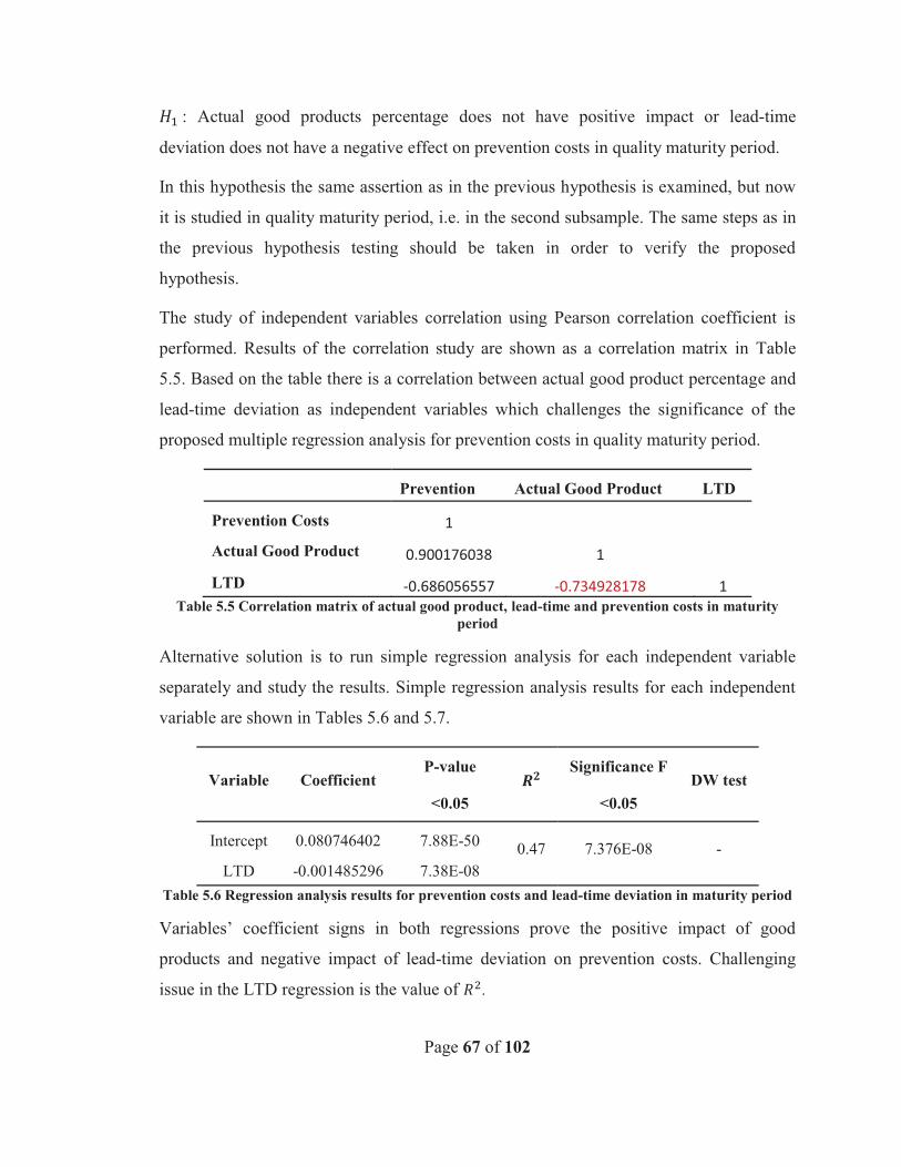
Page 67 of 102
: Actual good products percentage does not have positive impact or lead-time
deviation does not have a negative effect on prevention costs in quality maturity period.
In this hypothesis the same assertion as in the previous hypothesis is examined, but now
it is studied in quality maturity period, i.e. in the second subsample. The same steps as in
the previous hypothesis testing should be taken in order to verify the proposed
hypothesis.
The study of independent variables correlation using Pearson correlation coefficient is
performed. Results of the correlation study are shown as a correlation matrix in Table
5.5. Based on the table there is a correlation between actual good product percentage and
lead-time deviation as independent variables which challenges the significance of the
proposed multiple regression analysis for prevention costs in quality maturity period.
Prevention Actual Good Product LTD
Prevention Costs 1 Actual Good Product 0.900176038 1 LTD -0.686056557 -0.734928178 1
Table 5.5 Correlation matrix of actual good product, lead-time and prevention costs in maturity period
Alternative solution is to run simple regression analysis for each independent variable
separately and study the results. Simple regression analysis results for each independent
variable are shown in Tables 5.6 and 5.7.
Variable Coefficient P-value
<0.05
Significance F
<0.05 DW test
Intercept 0.080746402 7.88E-50 0.47 7.376E-08 - LTD -0.001485296 7.38E-08
Table 5.6 Regression analysis results for prevention costs and lead-time deviation in maturity period
Variables’ coefficient signs in both regressions prove the positive impact of good
products and negative impact of lead-time deviation on prevention costs. Challenging
issue in the LTD regression is the value of .
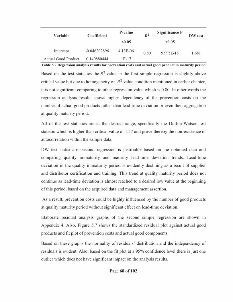
Page 68 of 102
Variable Coefficient P-value
<0.05
Significance F
<0.05 DW test
Intercept -0.046202896 4.13E-06 0.80 9.995E-18 1.681 Actual Good Product 0.140880444 1E-17
Table 5.7 Regression analysis results for prevention costs and actual good product in maturity period
Based on the test statistics the value in the first simple regression is slightly above
critical value but due to homogeneity of value condition mentioned in earlier chapter,
it is not significant comparing to other regression value which is 0.80. In other words the
regression analysis results shows higher dependency of the prevention costs on the
number of actual good products rather than lead-time deviation or even their aggregation
at quality maturity period.
All of the test statistics are at the desired range, specifically the Durbin-Watson test
statistic which is higher than critical value of 1.57 and prove thereby the non-existence of
autocorrelation within the sample data.
DW test statistic in second regression is justifiable based on the obtained data and
comparing quality immaturity and maturity lead-time deviation trends. Lead-time
deviation in the quality immaturity period is evidently declining as a result of supplier
and distributor certification and training. This trend at quality maturity period does not
continue as lead-time deviation is almost reached to a desired low value at the beginning
of this period, based on the acquired data and management assertion.
As a result, prevention costs could be highly influenced by the number of good products
at quality maturity period without significant effect on lead-time deviation.
Elaborate residual analysis graphs of the second simple regression are shown in
Appendix 4. Also, Figure 5.7 shows the standardized residual plot against actual good
products and fit plot of prevention costs and actual good components.
Based on these graphs the normality of residuals’ distribution and the independency of
residuals is evident. Also, based on the fit plot at a 95% confidence level there is just one
outlier which does not have significant impact on the analysis results.
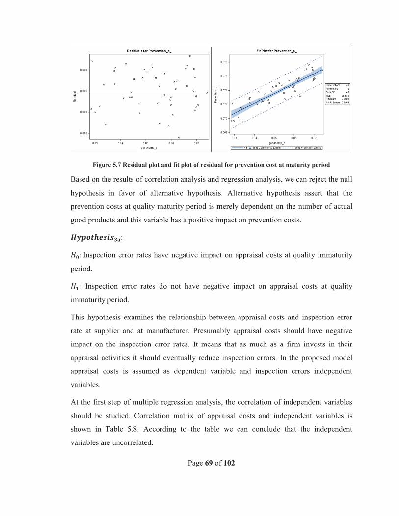
Page 69 of 102
Figure 5.7 Residual plot and fit plot of residual for prevention cost at maturity period
Based on the results of correlation analysis and regression analysis, we can reject the null
hypothesis in favor of alternative hypothesis. Alternative hypothesis assert that the
prevention costs at quality maturity period is merely dependent on the number of actual
good products and this variable has a positive impact on prevention costs.
:
Inspection error rates have negative impact on appraisal costs at quality immaturity
period.
Inspection error rates do not have negative impact on appraisal costs at quality
immaturity period.
This hypothesis examines the relationship between appraisal costs and inspection error
rate at supplier and at manufacturer. Presumably appraisal costs should have negative
impact on the inspection error rates. It means that as much as a firm invests in their
appraisal activities it should eventually reduce inspection errors. In the proposed model
appraisal costs is assumed as dependent variable and inspection errors independent
variables.
At the first step of multiple regression analysis, the correlation of independent variables
should be studied. Correlation matrix of appraisal costs and independent variables is
shown in Table 5.8. According to the table we can conclude that the independent
variables are uncorrelated.
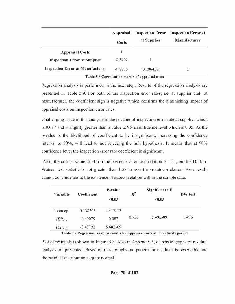
Page 70 of 102
Appraisal
Costs
Inspection Error
at Supplier
Inspection Error at
Manufacturer
Appraisal Costs 1 Inspection Error at Supplier -0.3402 1
Inspection Error at Manufacturer -0.8375 0.206458 1 Table 5.8 Corroleation martix of appraisal costs
Regression analysis is performed in the next step. Results of the regression analysis are
presented in Table 5.9. For both of the inspection error rates, i.e. at supplier and at
manufacturer, the coefficient sign is negative which confirms the diminishing impact of
appraisal costs on inspection error rates.
Challenging issue in this analysis is the p-value of inspection error rate at supplier which
is 0.087 and is slightly greater than p-value at 95% confidence level which is 0.05. As the
p-value is the likelihood of coefficient to be insignificant, increasing the confidence
interval to 90%, will lead to not rejecting the null hypothesis. It means that at 90%
confidence level the inspection error rate coefficient is significant.
Also, the critical value to affirm the presence of autocorrelation is 1.31, but the Durbin-
Watson test statistic is not greater than 1.57 to assert non-autocorrelation. As a result,
cannot conclude about the existence of autocorrelation within the sample data.
Variable Coefficient P-value
<0.05
Significance F
<0.05 DW test
Intercept 0.138703 4.41E-13 0.730 5.49E-09 1.496 -0.40079 0.087
-2.47792 5.68E-09 Table 5.9 Regression analysis results for appraisal costs at immaturity period
Plot of residuals is shown in Figure 5.8. Also in Appendix 5, elaborate graphs of residual
analysis are presented. Based on these graphs, no pattern for residuals is observable and
the residual distribution is quite normal.
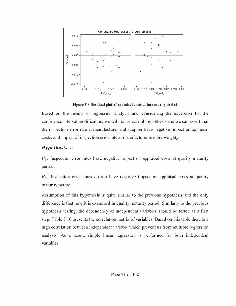
Page 71 of 102
Figure 5.8 Residual plot of appraisal costs at immaturity period
Based on the results of regression analysis and considering the exception for the
confidence interval modification, we will not reject null hypothesis and we can assert that
the inspection error rate at manufacturer and supplier have negative impact on appraisal
costs, and impact of inspection error rate at manufacturer is more weighty.
:
: Inspection error rates have negative impact on appraisal costs at quality maturity
period.
: Inspection error rates do not have negative impact on appraisal costs at quality
maturity period.
Assumption of this hypothesis is quite similar to the previous hypothesis and the only
difference is that now it is examined in quality maturity period. Similarly to the previous
hypothesis testing, the dependency of independent variables should be tested as a first
step. Table 5.10 presents the correlation matrix of variables. Based on this table there is a
high correlation between independent variable which prevent us from multiple regression
analysis. As a result, simple linear regression is performed for both independent
variables.
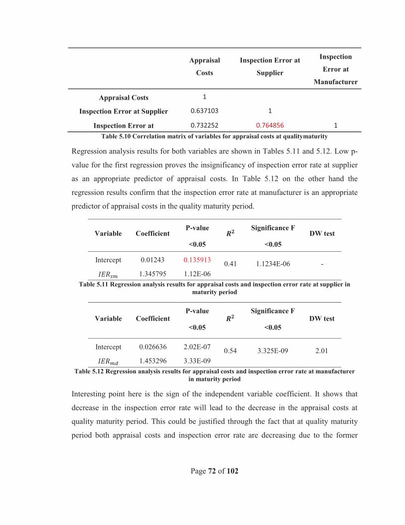
Page 72 of 102
Appraisal
Costs
Inspection Error at
Supplier
Inspection
Error at
Manufacturer
Appraisal Costs 1 Inspection Error at Supplier 0.637103 1
Inspection Error at 0.732252 0.764856 1 Table 5.10 Correlation matrix of variables for appraisal costs at qualitymaturity
Regression analysis results for both variables are shown in Tables 5.11 and 5.12. Low p-
value for the first regression proves the insignificancy of inspection error rate at supplier
as an appropriate predictor of appraisal costs. In Table 5.12 on the other hand the
regression results confirm that the inspection error rate at manufacturer is an appropriate
predictor of appraisal costs in the quality maturity period.
Variable Coefficient P-value
<0.05
Significance F
<0.05 DW test
Intercept 0.01243 0.135913 0.41 1.1234E-06 - 1.345795 1.12E-06
Table 5.11 Regression analysis results for appraisal costs and inspection error rate at supplier in maturity period
Variable Coefficient P-value
<0.05
Significance F
<0.05 DW test
Intercept 0.026636 2.02E-07 0.54 3.325E-09 2.01 1.453296 3.33E-09
Table 5.12 Regression analysis results for appraisal costs and inspection error rate at manufacturer in maturity period
Interesting point here is the sign of the independent variable coefficient. It shows that
decrease in the inspection error rate will lead to the decrease in the appraisal costs at
quality maturity period. This could be justified through the fact that at quality maturity
period both appraisal costs and inspection error rate are decreasing due to the former
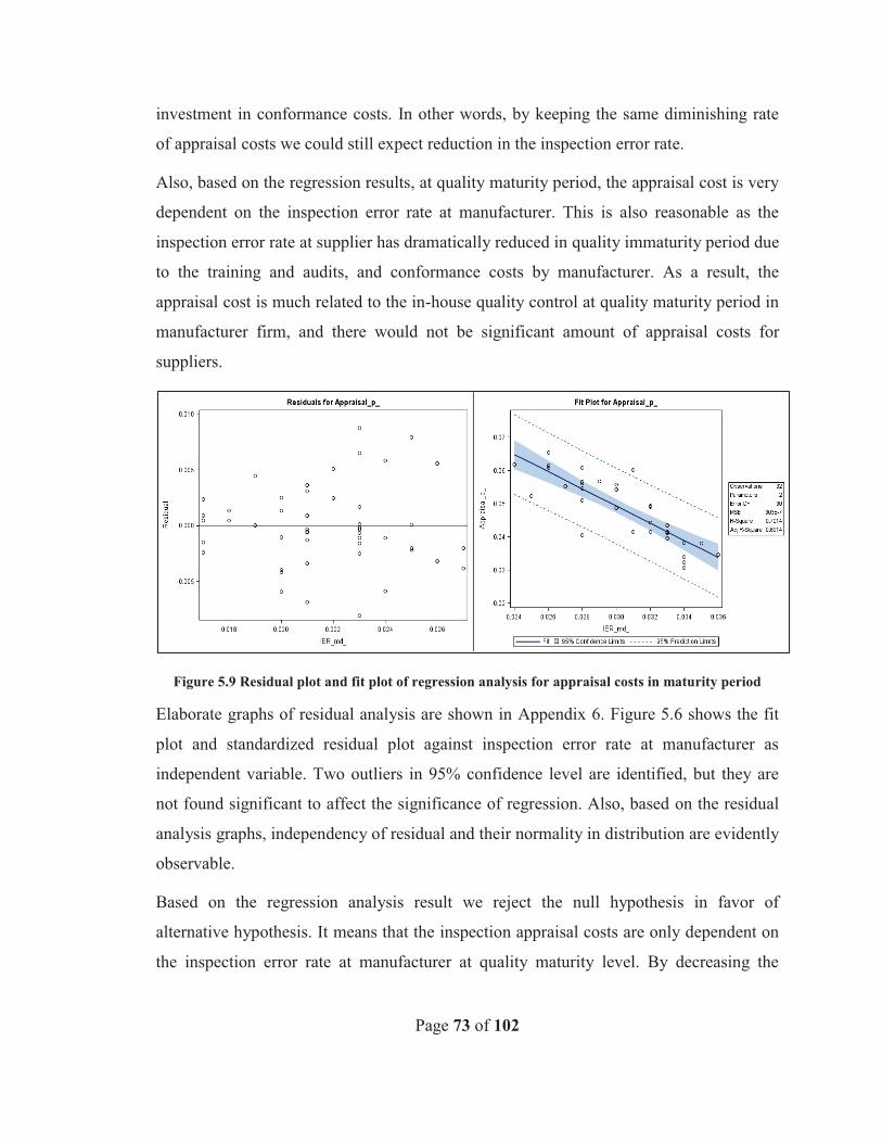
Page 73 of 102
investment in conformance costs. In other words, by keeping the same diminishing rate
of appraisal costs we could still expect reduction in the inspection error rate.
Also, based on the regression results, at quality maturity period, the appraisal cost is very
dependent on the inspection error rate at manufacturer. This is also reasonable as the
inspection error rate at supplier has dramatically reduced in quality immaturity period due
to the training and audits, and conformance costs by manufacturer. As a result, the
appraisal cost is much related to the in-house quality control at quality maturity period in
manufacturer firm, and there would not be significant amount of appraisal costs for
suppliers.
Figure 5.9 Residual plot and fit plot of regression analysis for appraisal costs in maturity period
Elaborate graphs of residual analysis are shown in Appendix 6. Figure 5.6 shows the fit
plot and standardized residual plot against inspection error rate at manufacturer as
independent variable. Two outliers in 95% confidence level are identified, but they are
not found significant to affect the significance of regression. Also, based on the residual
analysis graphs, independency of residual and their normality in distribution are evidently
observable.
Based on the regression analysis result we reject the null hypothesis in favor of
alternative hypothesis. It means that the inspection appraisal costs are only dependent on
the inspection error rate at manufacturer at quality maturity level. By decreasing the
Page 74 of 102
appraisal costs we can achieve the reduction in inspection error rate at manufacturer as a
result of former and continuous conformance activities.
:
Predicted internal failure cost is a good estimator of quality costs for both quality
maturity and immaturity periods.
Predicted internal failure cost is not a good estimator of quality costs for both quality
maturity and immaturity periods.
Predicted internal failure costs value could be calculated based on the Equation 4.19
presented in the model development chapter. It uses input parameters and decision
variables to estimate internal failure costs.
The model asserts that the predicted internal failure costs are a good estimator of actual
internal failure costs. Moreover, it is proposed that this is valid for any quality maturity
level. As a result the hypothesis testing is performed for whole sample once as the
predicted internal failure costs is nothing other than a function of decision and input
parameters.
In the model there are two components which comprise internal failure costs. The first
component is internal failure variable costs which are dependent to internal failure
predicted value, and the other component is internal failure fixed costs. In order to prove
that the proposed model is a good estimator, two conditions should be fulfilled in the
regression model. First, the independent variable should be a highly accurate predictor of
the dependent variable (i.e. the value of should be high), and, second, the value of the
intercept should be close to the internal failure fixed costs.
Table 5.13 shows the linear regression analysis results. As it shows predicted internal
failure costs have a positive correlation with internal failure costs. However, due to the
lack of historical data regarding internal failure fixed costs, we cannot have a conclusion
about the intercept value. From the statistics point of view, P-value and F value are
extremely above acceptable range and the value is very high, thus we can conclude
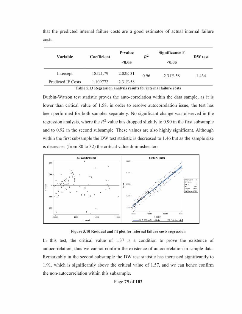
Page 75 of 102
that the predicted internal failure costs are a good estimator of actual internal failure
costs.
Variable Coefficient P-value
<0.05
Significance F
<0.05 DW test
Intercept 18521.79 2.02E-31 0.96 2.31E-58 1.434 Predicted IF Costs 1.109772 2.31E-58
Table 5.13 Regression analysis results for internal failure costs
Durbin-Watson test statistic proves the auto-correlation within the data sample, as it is
lower than critical value of 1.58. in order to resolve autocorrelation issue, the test has
been performed for both samples separately. No significant change was observed in the
regression analysis, where the value has dropped slightly to 0.90 in the first subsample
and to 0.92 in the second subsample. These values are also highly significant. Although
within the first subsample the DW test statistic is decreased to 1.46 but as the sample size
is decreases (from 80 to 32) the critical value diminishes too.
Figure 5.10 Residual and fit plot for internal failure costs regression
In this test, the critical value of 1.37 is a condition to prove the existence of
autocorrelation, thus we cannot confirm the existence of autocorrelation in sample data.
Remarkably in the second subsample the DW test statistic has increased significantly to
1.91, which is significantly above the critical value of 1.57, and we can hence confirm
the non-autocorrelation within this subsample.
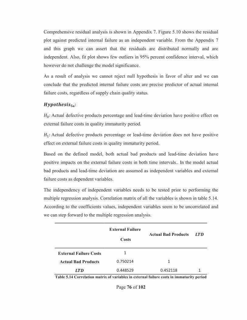
Page 76 of 102
Comprehensive residual analysis is shown in Appendix 7. Figure 5.10 shows the residual
plot against predicted internal failure as an independent variable. From the Appendix 7
and this graph we can assert that the residuals are distributed normally and are
independent. Also, fit plot shows few outliers in 95% percent confidence interval, which
however do not challenge the model significance.
As a result of analysis we cannot reject null hypothesis in favor of alter and we can
conclude that the predicted internal failure costs are precise predictor of actual internal
failure costs, regardless of supply chain quality status.
Actual defective products percentage and lead-time deviation have positive effect on
external failure costs in quality immaturity period.
Actual defective products percentage or lead-time deviation does not have positive
effect on external failure costs in quality immaturity period.
Based on the defined model, both actual bad products and lead-time deviation have
positive impacts on the external failure costs in both time intervals.. In the model actual
bad products and lead-time deviation are assumed as independent variables and external
failure costs as dependent variables.
The independency of independent variables needs to be tested prior to performing the
multiple regression analysis. Correlation matrix of all the variables is shown in table 5.14.
According to the coefficients values, independent variables seem to be uncorrelated and
we can step forward to the multiple regression analysis.
External Failure
Costs Actual Bad Products
External Failure Costs 1 Actual Bad Products 0.750214 1
0.448529 0.452118 1 Table 5.14 Correlation matrix of variables in external failure costs in immaturity period
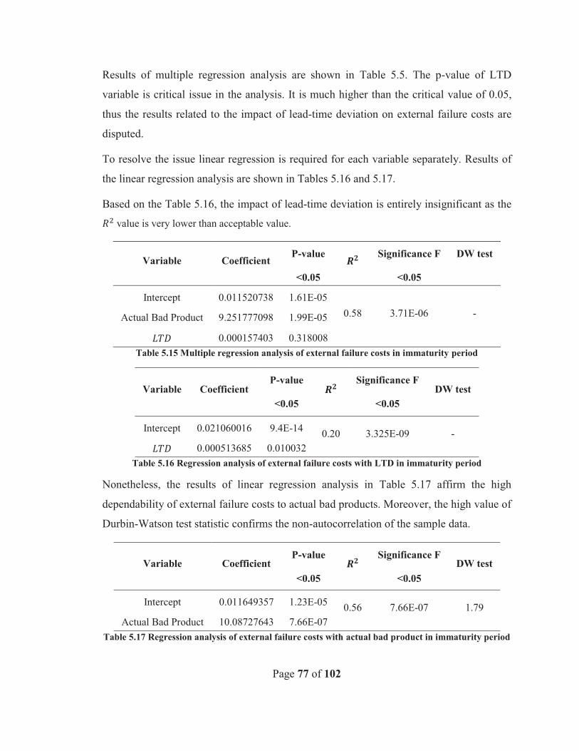
Page 77 of 102
Results of multiple regression analysis are shown in Table 5.5. The p-value of LTD
variable is critical issue in the analysis. It is much higher than the critical value of 0.05,
thus the results related to the impact of lead-time deviation on external failure costs are
disputed.
To resolve the issue linear regression is required for each variable separately. Results of
the linear regression analysis are shown in Tables 5.16 and 5.17.
Based on the Table 5.16, the impact of lead-time deviation is entirely insignificant as the
value is very lower than acceptable value.
Variable Coefficient P-value
<0.05
Significance F
<0.05
DW test
Intercept 0.011520738 1.61E-05 0.58 3.71E-06 - Actual Bad Product 9.251777098 1.99E-05
0.000157403 0.318008 Table 5.15 Multiple regression analysis of external failure costs in immaturity period
Variable Coefficient P-value
<0.05
Significance F
<0.05 DW test
Intercept 0.021060016 9.4E-14 0.20 3.325E-09 - 0.000513685 0.010032
Table 5.16 Regression analysis of external failure costs with LTD in immaturity period
Nonetheless, the results of linear regression analysis in Table 5.17 affirm the high
dependability of external failure costs to actual bad products. Moreover, the high value of
Durbin-Watson test statistic confirms the non-autocorrelation of the sample data.
Variable Coefficient P-value
<0.05
Significance F
<0.05 DW test
Intercept 0.011649357 1.23E-05 0.56 7.66E-07 1.79 Actual Bad Product 10.08727643 7.66E-07
Table 5.17 Regression analysis of external failure costs with actual bad product in immaturity period
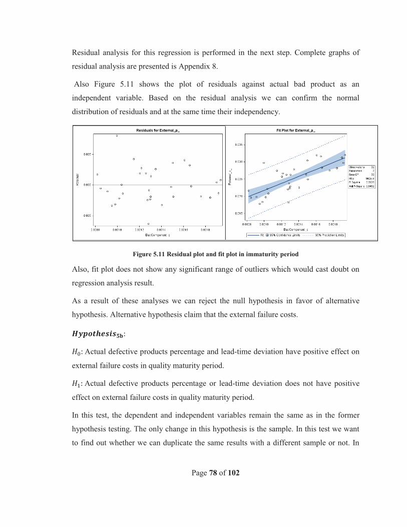
Page 78 of 102
Residual analysis for this regression is performed in the next step. Complete graphs of
residual analysis are presented is Appendix 8.
Also Figure 5.11 shows the plot of residuals against actual bad product as an
independent variable. Based on the residual analysis we can confirm the normal
distribution of residuals and at the same time their independency.
Figure 5.11 Residual plot and fit plot in immaturity period
Also, fit plot does not show any significant range of outliers which would cast doubt on
regression analysis result.
As a result of these analyses we can reject the null hypothesis in favor of alternative
hypothesis. Alternative hypothesis claim that the external failure costs.
Actual defective products percentage and lead-time deviation have positive effect on
external failure costs in quality maturity period.
Actual defective products percentage or lead-time deviation does not have positive
effect on external failure costs in quality maturity period.
In this test, the dependent and independent variables remain the same as in the former
hypothesis testing. The only change in this hypothesis is the sample. In this test we want
to find out whether we can duplicate the same results with a different sample or not. In
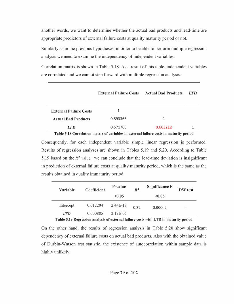
Page 79 of 102
another words, we want to determine whether the actual bad products and lead-time are
appropriate predictors of external failure costs at quality maturity period or not.
Similarly as in the previous hypotheses, in order to be able to perform multiple regression
analysis we need to examine the independency of independent variables.
Correlation matrix is shown in Table 5.18. As a result of this table, independent variables
are correlated and we cannot step forward with multiple regression analysis.
External Failure Costs Actual Bad Products
External Failure Costs 1 Actual Bad Products 0.893366 1
0.571766 0.663212 1 Table 5.18 Correlation matrix of variables in external failure costs in maturity period
Consequently, for each independent variable simple linear regression is performed.
Results of regression analyses are shown in Tables 5.19 and 5.20. According to Table
5.19 based on the value, we can conclude that the lead-time deviation is insignificant
in prediction of external failure costs at quality maturity period, which is the same as the
results obtained in quality immaturity period.
Variable Coefficient P-value
<0.05
Significance F
<0.05 DW test
Intercept 0.012204 2.44E-18 0.32 0.00002 - 0.000885 2.19E-05
Table 5.19 Regression analysis of external failure costs with LTD in maturity period
On the other hand, the results of regression analysis in Table 5.20 show significant
dependency of external failure costs on actual bad products. Also with the obtained value
of Durbin-Watson test statistic, the existence of autocorrelation within sample data is
highly unlikely.
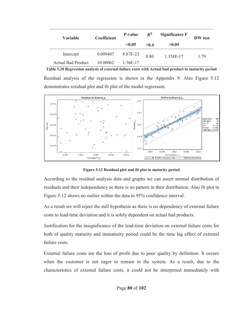
Page 80 of 102
Variable Coefficient P-value
>0.05
>0.4
Significance F
>0.05 DW test
Intercept 0.009407 8.87E-23 0.80 1.358E-17 1.79 Actual Bad Product 10.00062 1.36E-17
Table 5.20 Regression analysis of external failure costs with Actual bad product in maturity period
Residual analysis of the regression is shown in the Appendix 9. Also Figure 5.12
demonstrates residual plot and fit plot of the model regression.
Figure 5.12 Residual plot and fit plot in maturity period
According to the residual analysis data and graphs we can assert normal distribution of
residuals and their independency as there is no pattern in their distribution. Also fit plot in
Figure 5.12 shows no outlier within the data in 95% confidence interval.
As a result we will reject the null hypothesis as there is no dependency of external failure
costs to lead-time deviation and it is solely dependent on actual bad products.
Justification for the insignificance of the lead-time deviation on external failure costs for
both of quality maturity and immaturity period could be the time lag effect of external
failure costs.
External failure costs are the loss of profit due to poor quality by definition. It occurs
when the customer is not eager to remain in the system. As a result, due to the
characteristics of external failure costs, it could not be interpreted immediately with
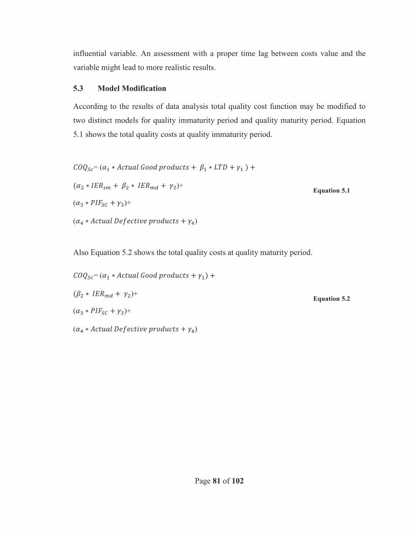
Page 81 of 102
influential variable. An assessment with a proper time lag between costs value and the
variable might lead to more realistic results.
5.3 Model Modification
According to the results of data analysis total quality cost function may be modified to
two distinct models for quality immaturity period and quality maturity period. Equation
5.1 shows the total quality costs at quality immaturity period.
= (
)+
( )+
( )
Equation 5.1
Also Equation 5.2 shows the total quality costs at quality maturity period.
= (
)+
( )+
( )
Equation 5.2
Page 82 of 102
6. Summary and Conclusions In this research we have developed a mathematical model which could predict the total
quality costs at different quality levels in manufacturing supply chain. Proposed model is
examined and validated against manufacturing supply chain data in two intervals, which
we call quality immaturity and quality maturity periods, respectively. The PAF
classification of quality costs has been used to develop mathematical model for total
quality costs. The definition of quality level is based on the definition of quality level in
the product supply chain. Based on the results the quality level is increasing when the
COQ increases in quality maturity period and, also, increments in quality level are not
necessarily accompanied by higher quality costs in quality maturity period.
Prevention cost group is different in quality immaturity and quality maturity periods. The
investment in prevention activities in quality immaturity period has a drastic role in lead-
time reduction, but due to the quality excellence in maturity period lead-time variation
would be insignificant and prevention costs at this period is solely dependent on the
number of actual good products.
In the appraisal costs category, the inspection error rates at manufacturer and supplier
have impact on appraisal costs in quality immaturity period, but inspection error rate at
supplier is not significant at quality maturity period as supplier evaluation and
certification occur in immaturity period. As a result, appraisal costs would be merely
dependent on inspection errors at manufacturer at maturity period, and surprisingly they
decrease simultaneously as a result of continuous improvement efforts.
Furthermore, according to the data analysis results, predicted internal failure costs are a
precise estimator of total internal failure costs regardless of quality excellence status. In
another words, the predicted amount of internal failure costs could be assumed as internal
failure variable costs.
Finally, contrary to our hypothesis, external failure costs are merely dependent on the
actual number of bad products which reach to the hand of customers, and they are not
dependent on the lead-time deviation in any quality maturity status. As it was proposed in
Page 83 of 102
the data analysis chapter to observe the impact of lead-time deviation on external failure
costs it is recommended to study their relationships in time lags.
6.1 Future works
Considering the model assumptions and limitations, future works could be lied in
different ways. Consideration of model for variant demand condition and integrating
demand forecasting techniques in COQ could be one of the alternatives. Also,
modification of quality level definition to include more quality dimensions is another
possible key point remaining for future investigation. Furthermore, the proposed model
is suitable for currently established supply chain, thus the cost of switching between
suppliers and distributers or retailers is not considered in the model development.
.Subsequently the consideration of cost of switching between supply chain entities is
another work that can be done in future. Moreover, inventory costs as a quality issue
could be deliberated in future works, because due to the the available data they were
completely omitted in this work. Finally, in the context of data analysis, utilizing
robustness test and techniques will enhance analysis results validity. This could be done
through random continuous event simulation or any other statistical tool.

Page 84 of 102
Bibliography
ABDUL-KADER, W., GANJAVI, O. and SOLAIMAN, A., 2010. An integrated model
for optimisation of production and quality costs. International Journal of Production
Research, 48(24), pp. 7357-7370.
AL-TMEEMY, S.M.H., RAHMAN, H.A. and HARUN, Z., 2012. Contractors' perception
of the use of costs of quality system in Malaysian building construction projects.
International Journal of Project Management, 30(7), pp. 827-838.
ALZAMAN, C., RAMUDHIN, A. and BULGAK, A.A., 2009. Heuristic procedures to
solve a binary nonlinear supply chain model: A casestudy from the aerospace industry,
2009 International Conference on Computers and Industrial Engineering, CIE 2009
2009, pp. 985-990.
BANASIK, M., 2009. A study of the costs of quality in a renewable resource
environment.
BERUVIDES, M.G. and CHIU, Y.D., 2003. The economic inflection point – A new tool
for decision making of quality improvement programs, Proceedings of the 24th Annual
National Conference of the American Society for Engineering Management 2003, pp.
346-353.
BLANK, L. and SOLORZANO, J., 1978. USING QUALITY COST ANALYSIS FOR
MANAGEMENT IMPROVEMENT. Ind Eng, 10(2), pp. 46-51.
BURGESS, T., 1996. Modelling quality-cost dynamics. International Journal of Quality
& Reliability Management, 13(3), pp. 8-26.
CAMPANELLA, J. and CORCORAN, F., 1983. Principles of Quality Costs. Ideas and
Applications, 1, pp. 563.
Page 85 of 102
CARR, L.P., 1992. Applying cost of quality to a service business, Sloan Management
Review 1992.
CASTILLO-VILLAR, K.K., SMITH, N.R. and SIMONTON, J.L., 2012. A model for
supply chain design considering the cost of quality. Applied Mathematical Modelling,
36(12), pp. 5920-5935.
CASTILLO-VILLAR, K.K., SMITH, N.R. and SIMONTONCY, J.L., 2012. The impact
of the cost of quality on serial supply-chain network design. International Journal of
Production Research, 50(19), pp. 5544-5566.
CHEAH, S.-., MD. SHAHBUDIN, A.S. and MD. TAIB, F., 2011. Tracking hidden
quality costs in a manufacturing company: An action research. International Journal of
Quality and Reliability Management, 28(4), pp. 405-425.
CLARK, H.J. and TANNOCK, J.D.T., 1999. The development and implementation of a
simulation tool for the assessment of quality economics within a cell-based
manufacturing company. International Journal of Production Research, 37(5), pp. 979-
995.
COOPER, R. and KAPLAN, R.S., 1988. Measure costs right: make the right decisions.
Harvard business review, 66(5), pp. 96-103.
DALE, B.G. and PLUNKETT, J.J., 1999. Quality costing. Gower Publishing, Ltd.
DE RUYTER, A.S., CARDEW-HALL, M.J. and HODGSON, P.D., 2002. Estimating
quality costs in an automotive stamping plant through the use of simulation. International
Journal of Production Research, 40(15 SPEC.), pp. 3835-3848.
DEMING, W.E., 1986. Out of the crisis. Cambridge, MA: Massachusetts Institute of
Technology. Center for Advanced Engineering Study, , pp. 6.
Page 86 of 102
DESAI, D.A., 2008. Cost of quality in small- and medium-sized enterprises: Case of an
Indian engineering company. Production Planning and Control, 19(1), pp. 25-34.
DROR, S., 2010. A methodology for realignment of quality cost elements. Journal of
Modelling in Management, 5(2), pp. 142-157.
FEIGENBAUM, A.V., 1956. Total quality Control. Harvard business review, 34(6), pp.
93-101.
FINE, C.H., 1986. Quality improvement and learning in productive systems.
Management Science, 32(10), pp. 1301-1315.
FOX, M., 1989. The great economic quality hoax. Quality Assurance, 15(2), pp. 72.
FREIESLEBEN, J., 2004. On the limited value of Cost of Quality Models. Total Quality
Management and Business Excellence, 15(7), pp. 959-969.
GARDNER, L.L., GRANT, M.E. and ROLSTON, L.J., 1995. Using simulation to assess
costs of quality, Winter Simulation Conference Proceedings 1995, pp. 945-951.
GARVIN, D.A., 1996. Competing on the eight dimensions of quality. IEEE Engineering
Management Review, 24(1), pp. 15-23.
GODFREY, J.T. and PASEWARK, W., 1988. Controlling quality costs. Management
Accounting, 77, pp. 48-51.
GOULDEN, C. and RAWLINS, L., 1995. A hybrid model for process quality costing.
International Journal of Quality & Reliability Management, 12(8), pp. 32-47.
HARRINGTON, H.J., 1987. Poor-quality cost. M. Dekker.
ITTNER, C.D., 1996. Exploratory evidence on the behavior of quality costs. Operations
research, 44(1), pp. 114-130.
Page 87 of 102
JURAN, J.M., ed, 1962. Quality Control Handbook. 1st edn. New york, NY: McGraw-
Hill.
JURAN, J.M., 1951. Quality Control Handbook. New York, NY: McGraw-Hill.
JURAN, J.M. and GRYNA, F.M., 1993. Quality planning and analysis: from product
development through use. New York: McGraw-Hill.
KIANI, B., SHIROUYEHZAD, H., BAFTI, F.K. and FOULADGAR, H., 2009. System
dynamics approach to analysing the cost factors effects on cost of quality. International
Journal of Quality and Reliability Management, 26(7), pp. 685-698.
MACHOWSKI, F. and DALE, B.G., 1998. Quality costing: An examination of
knowledge, attitudes, and perceptions. Quality Management Journal, 5(3),.
MAHANTY, B., NAIKAN, V. and NATH, T., 2012. System Dynamics Approach for
Modeling Cost of Quality. International Journal of performability Engineering, 8(6), pp.
625.
MARCELLUS, R.L. and DADA, M., 1991. Interactive process quality improvement.
Management Science, 37(11), pp. 1365-1376.
MARSH, J., 1989. Process modeling for quality improvement, Proceedings of the Second
International Conference on Total Quality Management 1989, McGraw-Hill, pp. 16.
MAXWELL, S.E., 2000. Sample size and multiple regression analysis. Psychological
methods, 5(4), pp. 434.
MILLER, J.R. and MORRIS, J.S., 2000. Is quality free or profitable? Quality Progress,
33(1), pp. 50-53.
NOZ, W., REDDING, B. and WARE, P., 1989. The Quality Manager's Job: Optimize
Costs. Quality Costs: Ideas and Applications, 1, pp. 53-60.
Page 88 of 102
OMAR, M.K., MURUGAN, S., AKRAMIN, N. and MUHAMAD, M.R., 2010. Cost of
quality modeling: Extension and improvement, IEEM2010 - IEEE International
Conference on Industrial Engineering and Engineering Management 2010, pp. 1849-
1853.
OMAR, M.K., SIM, H.K., MURUGAN, S. and MUHAMAD, M.R., 2009. The impact of
costs of quality: A simulation approach, Industrial Engineering and Engineering
Management, 2009. IEEM 2009. IEEE International Conference on 2009, pp. 1327-1331.
PLUNKETT, J.J. and DALE, B.G., 1988. Quality costs: a critique of some 'economic
cost of quality' models. International Journal of Production Research, 26(11), pp. 1713-
1726.
PORTER, L.J. and RAYNER, P., 1992. Quality costing for total quality management.
International Journal of Production Economics, 27(1), pp. 69-81.
RAMUDHIN, A., ALZAMAN, C. and BULGAK, A.A., 2008. Incorporating the cost of
quality in supply chain design. Journal of Quality in Maintenance Engineering, 14(1), pp.
71-86.
SANDOVAL-CHÁVEZ, D.A. and BERUVIDES, M.G., 1998. Using opportunity costs
to determine the cost of quality: a case study in a continuous-process industry. The
Engineering Economist, 43(2), pp. 107-124.
SCHIFFAUEROVA, A. and THOMSON, V., 2006. A review of research on cost of
quality models and best practices. International Journal of Quality and Reliability
Management, 23(6), pp. 647-669.
SCHNEIDERMAN, A.M., 1986. Optimum quality costs and zero defects: are they
contradictory concepts? Quality Progress, 19(11), pp. 28-31.
SHANK, J.K. and GOVINDARAJAN, V., 1994. Measuring the cost of quality: A
strategic cost management perspective. Journal of Cost Management, 8(2), pp. 5-17.
Page 89 of 102
SIM, H.K., OMAR, M.K., JACKIE, Y.J.K. and BONG, C.S., 2009. Cost of quality for an
automotive industry: A survey and findings. International Journal of Manufacturing
Technology and Management, 17(4), pp. 437-452.
SOWER, V.E., QUARLES, R. and BROUSSARD, E., 2007. Cost of quality usage and
its relationship to quality system maturity. International Journal of Quality and
Reliability Management, 24(2), pp. 121-140.
SRIVASTAVA, S.K., 2008. Towards estimating Cost of Quality in supply chains. Total
Quality Management and Business Excellence, 19(3), pp. 193-208.
SU, Q., SHI, J.-. and LAI, S.-., 2009. Research on the trade-off relationship within
quality costs: A case study. Total Quality Management and Business Excellence, 20(12),
pp. 1395-1405.
TATIKONDA, L.U. and TATIKONDA, R.J., 1996. Measuring and reporting the cost of
quality. Production and Inventory Management Journal, 37, pp. 1-7.
TSAI, W., 1998. Quality cost measurement under activity-based costing. International
Journal of Quality & Reliability Management, 15(7), pp. 719-752.
TSAI, W.-. and HSU, W., 2010. A novel hybrid model based on DEMATEL and ANP
for selecting cost of quality model development. Total Quality Management and Business
Excellence, 21(4), pp. 439-456.
TYE, L.H., HALIM, H.A. and RAMAYAH, T., 2011. An exploratory study on cost of
quality implementation in Malaysia: The case of penang manufacturing firms. Total
Quality Management and Business Excellence, 22(12), pp. 1299-1315.
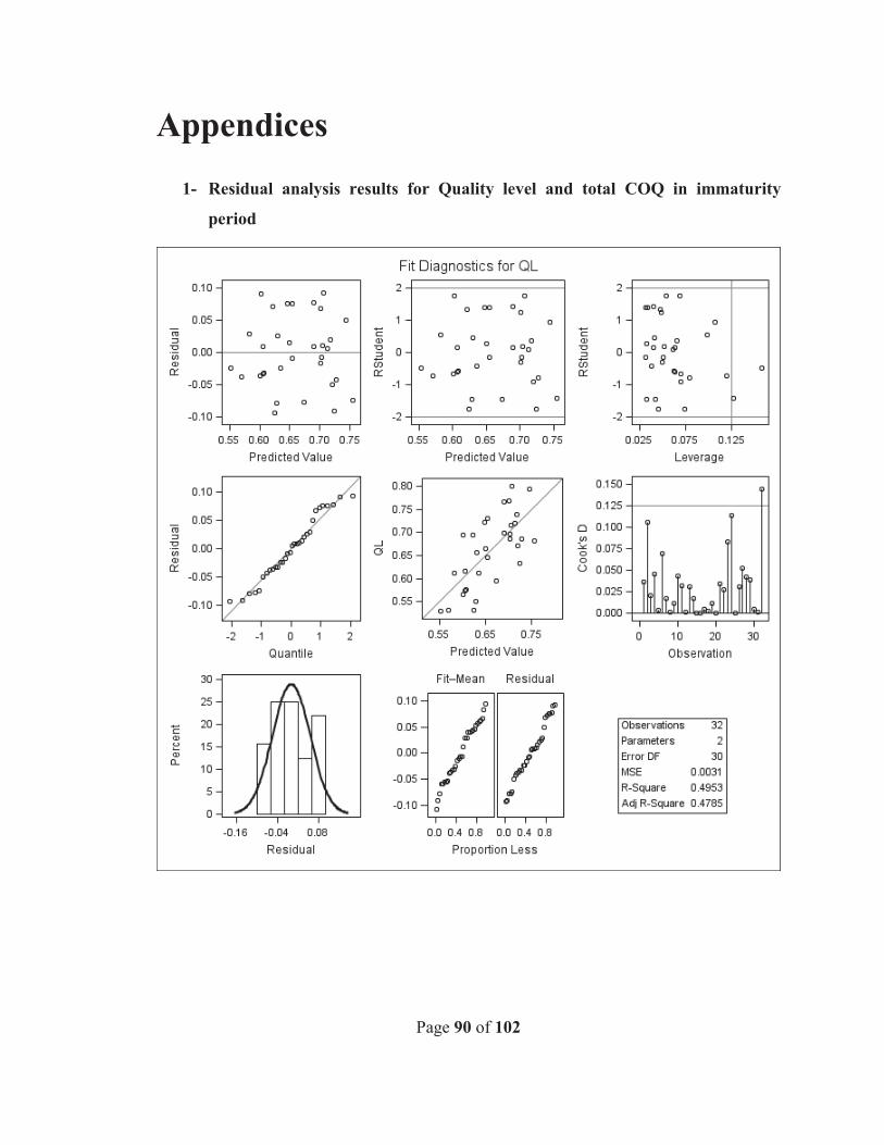
Page 90 of 102
Appendices
1- Residual analysis results for Quality level and total COQ in immaturity
period
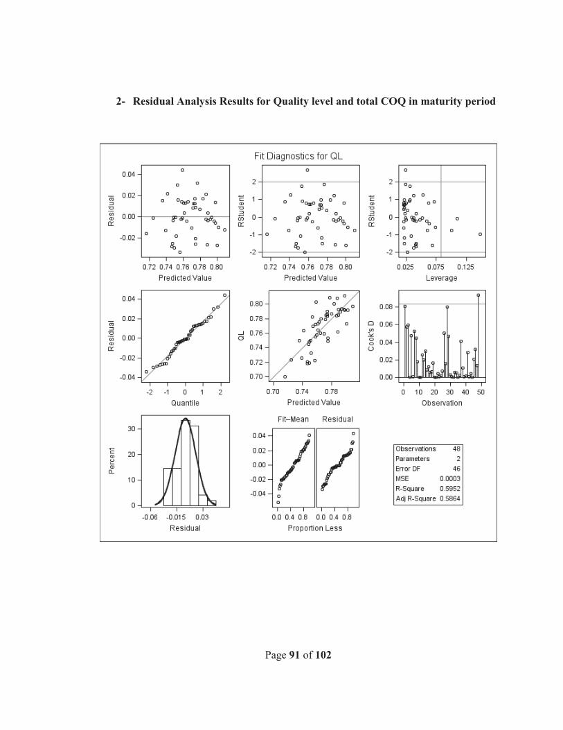
Page 91 of 102
2- Residual Analysis Results for Quality level and total COQ in maturity period
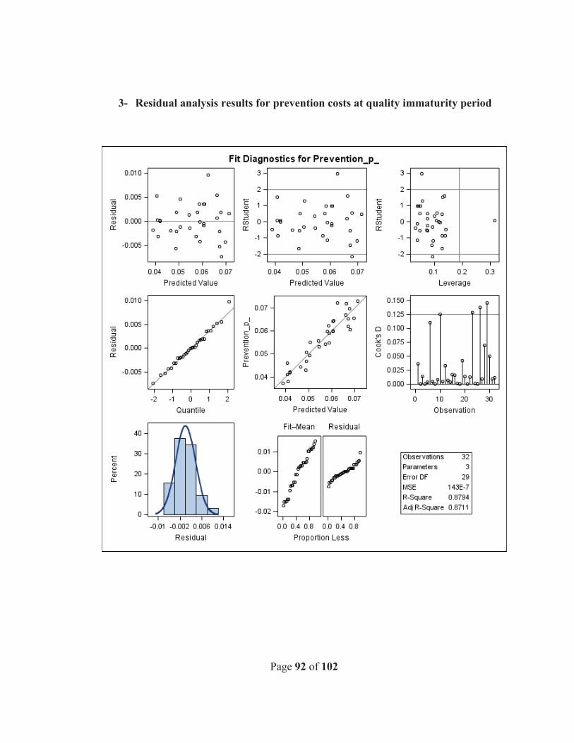
Page 92 of 102
3- Residual analysis results for prevention costs at quality immaturity period
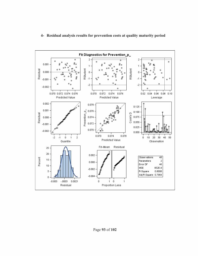
Page 93 of 102
4- Residual analysis results for prevention costs at quality maturity period
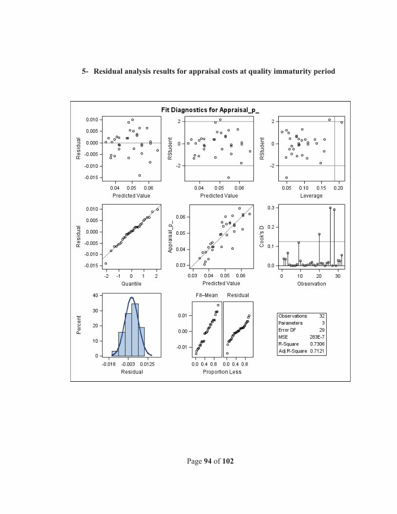
Page 94 of 102
5- Residual analysis results for appraisal costs at quality immaturity period
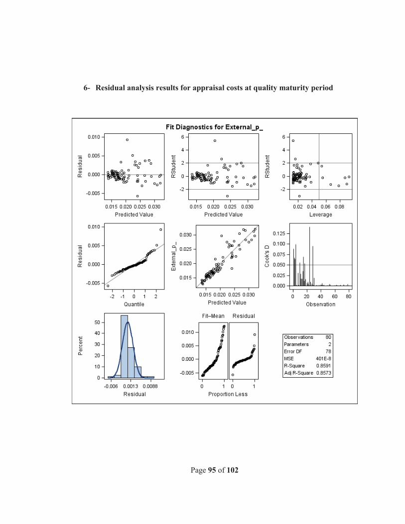
Page 95 of 102
6- Residual analysis results for appraisal costs at quality maturity period
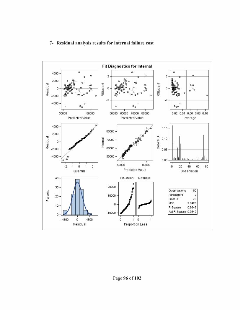
Page 96 of 102
7- Residual analysis results for internal failure cost
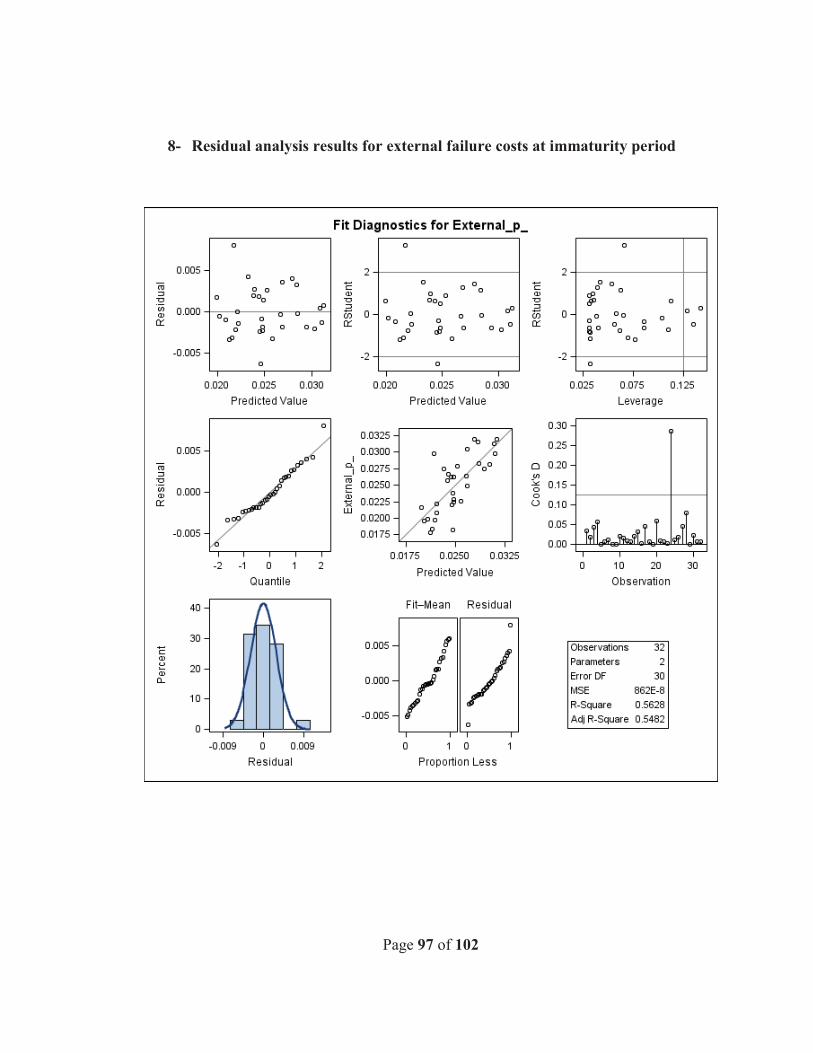
Page 97 of 102
8- Residual analysis results for external failure costs at immaturity period
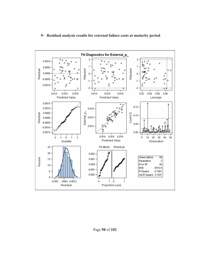
Page 98 of 102
9- Residual analysis results for external failure costs at maturity period
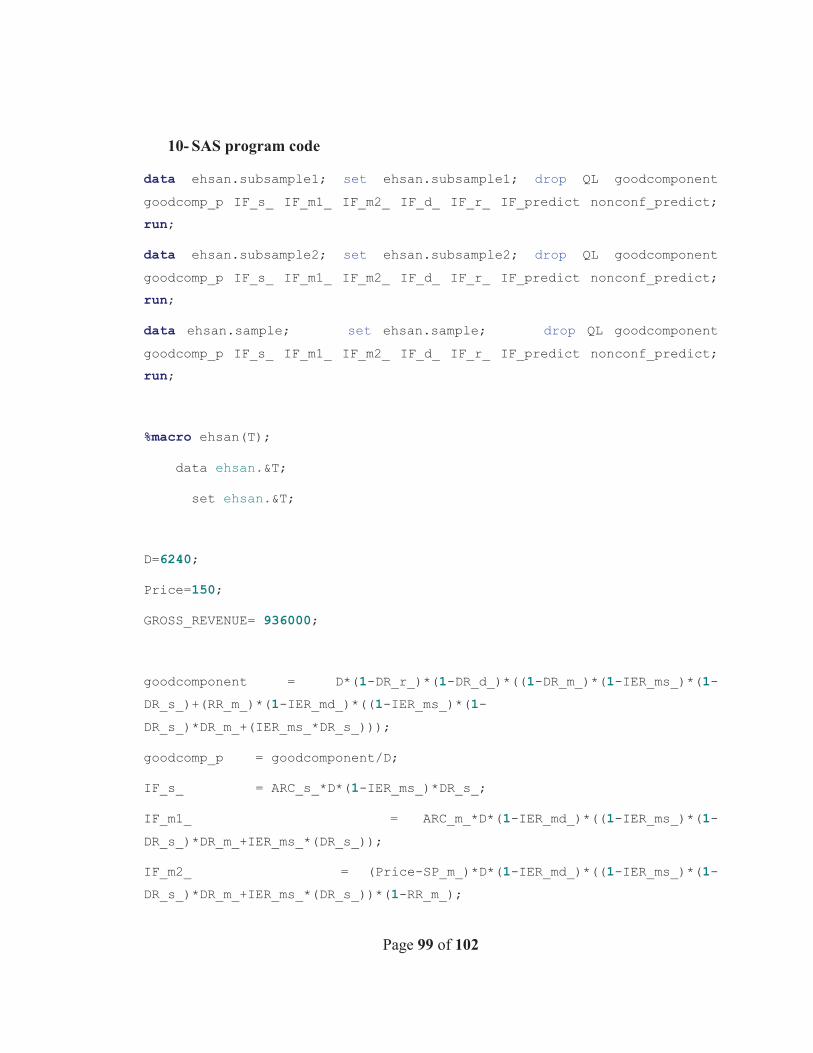
Page 99 of 102
10- SAS program code
data ehsan.subsample1; set ehsan.subsample1; drop QL goodcomponent
goodcomp_p IF_s_ IF_m1_ IF_m2_ IF_d_ IF_r_ IF_predict nonconf_predict;
run; data ehsan.subsample2; set ehsan.subsample2; drop QL goodcomponent
goodcomp_p IF_s_ IF_m1_ IF_m2_ IF_d_ IF_r_ IF_predict nonconf_predict;
run; data ehsan.sample; set ehsan.sample; drop QL goodcomponent goodcomp_p IF_s_ IF_m1_ IF_m2_ IF_d_ IF_r_ IF_predict nonconf_predict;
run;
%macro ehsan(T); data ehsan.&T;
set ehsan.&T;
D=6240; Price=150; GROSS_REVENUE= 936000;
goodcomponent = D*(1-DR_r_)*(1-DR_d_)*((1-DR_m_)*(1-IER_ms_)*(1-DR_s_)+(RR_m_)*(1-IER_md_)*((1-IER_ms_)*(1-DR_s_)*DR_m_+(IER_ms_*DR_s_)));
goodcomp_p = goodcomponent/D;
IF_s_ = ARC_s_*D*(1-IER_ms_)*DR_s_; IF_m1_ = ARC_m_*D*(1-IER_md_)*((1-IER_ms_)*(1-DR_s_)*DR_m_+IER_ms_*(DR_s_));
IF_m2_ = (Price-SP_m_)*D*(1-IER_md_)*((1-IER_ms_)*(1-DR_s_)*DR_m_+IER_ms_*(DR_s_))*(1-RR_m_);
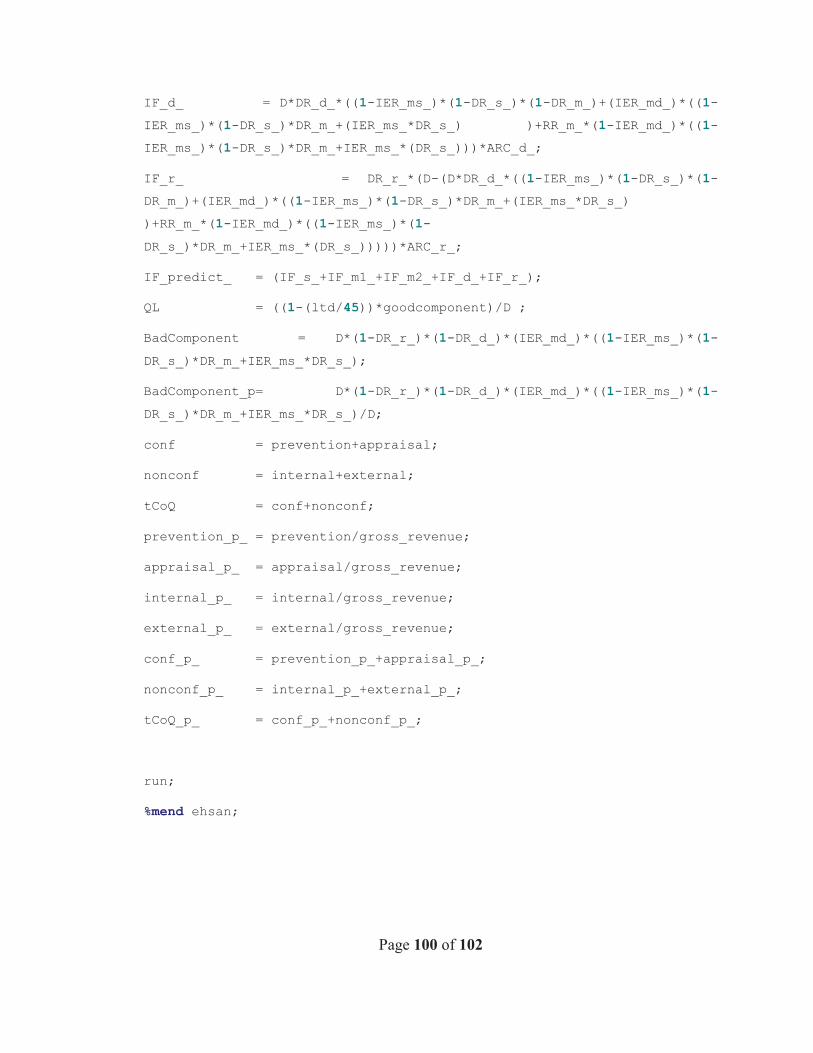
Page 100 of 102
IF_d_ = D*DR_d_*((1-IER_ms_)*(1-DR_s_)*(1-DR_m_)+(IER_md_)*((1-IER_ms_)*(1-DR_s_)*DR_m_+(IER_ms_*DR_s_) )+RR_m_*(1-IER_md_)*((1-IER_ms_)*(1-DR_s_)*DR_m_+IER_ms_*(DR_s_)))*ARC_d_; IF_r_ = DR_r_*(D-(D*DR_d_*((1-IER_ms_)*(1-DR_s_)*(1-DR_m_)+(IER_md_)*((1-IER_ms_)*(1-DR_s_)*DR_m_+(IER_ms_*DR_s_) )+RR_m_*(1-IER_md_)*((1-IER_ms_)*(1-DR_s_)*DR_m_+IER_ms_*(DR_s_)))))*ARC_r_;
IF_predict_ = (IF_s_+IF_m1_+IF_m2_+IF_d_+IF_r_);
QL = ((1-(ltd/45))*goodcomponent)/D ; BadComponent = D*(1-DR_r_)*(1-DR_d_)*(IER_md_)*((1-IER_ms_)*(1-DR_s_)*DR_m_+IER_ms_*DR_s_);
BadComponent_p= D*(1-DR_r_)*(1-DR_d_)*(IER_md_)*((1-IER_ms_)*(1-DR_s_)*DR_m_+IER_ms_*DR_s_)/D;
conf = prevention+appraisal;
nonconf = internal+external;
tCoQ = conf+nonconf;
prevention_p_ = prevention/gross_revenue;
appraisal_p_ = appraisal/gross_revenue;
internal_p_ = internal/gross_revenue;
external_p_ = external/gross_revenue;
conf_p_ = prevention_p_+appraisal_p_;
nonconf_p_ = internal_p_+external_p_;
tCoQ_p_ = conf_p_+nonconf_p_;
run;
%mend ehsan;
Page 101 of 102
*************************
*** REGRESSIONS *********
************************;
%macro REG_all(T); proc reg data=ehsan.&T; model internal = IF_predict_
/dw; run;
proc reg data=ehsan.&T; model Prevention_p_ = goodcomp_p LTD
/dw; run;
proc reg data=ehsan.&T; model Prevention_p_ = goodcomp_p
/dw; run; *only for subsample2;
proc reg data=ehsan.&T; model appraisal_p_ = IER_ms_ IER_md_
/dw; run;
proc reg data=ehsan.&T; model appraisal_p_ = IER_md_
/dw; run; *only for subsample2;
proc reg data=ehsan.&T; model appraisal_p_ = IER_ms_
/dw; run; *only for subsample2;
proc reg data=ehsan.&T; model external_p_ = BadComponent_p LTD
/dw; run;
proc reg data=ehsan.&T; model external_p_ = BadComponent_p
/dw; run;
%mend REG_all;
%macro REG_1(T); proc reg data=ehsan.&T; model internal = IF_predict_
/dw; run;
proc reg data=ehsan.&T; model Prevention_p_ = goodcomp_p LTD
/dw; run;
proc reg data=ehsan.&T; model Prevention_p_ = goodcomp_p
/dw; run; *only for subsample2;
Page 102 of 102
proc reg data=ehsan.&T; model appraisal_p_ = IER_ms_ IER_md_
/dw; run;
proc reg data=ehsan.&T; model appraisal_p_ = IER_md_
/dw; run; *only for subsample2;
proc reg data=ehsan.&T; model appraisal_p_ = IER_ms_
/dw; run; *only for subsample2;
proc reg data=ehsan.&T; model external_p_ = BadComponent_p LTD
/dw; run;
proc reg data=ehsan.&T; model external_p_ = BadComponent_p
/dw; run;
%mend REG_1;
%macro REG_2(T); proc reg data=ehsan.&T; model internal = IF_predict_
/dw; run;
proc reg data=ehsan.&T; model Prevention_p_ = goodcomp_p LTD
/dw; run;
proc reg data=ehsan.&T; model Prevention_p_ = goodcomp_p
/dw; run; *only for subsample2;
proc reg data=ehsan.&T; model appraisal_p_ = IER_ms_ IER_md_
/dw; run;
proc reg data=ehsan.&T; model appraisal_p_ = IER_md_
/dw; run; *only for subsample2;
proc reg data=ehsan.&T; model appraisal_p_ = IER_ms_
/dw; run; *only for subsample2;
proc reg data=ehsan.&T; model external_p_ = BadComponent_p LTD
/dw; run;
proc reg data=ehsan.&T; model external_p_ = BadComponent_p
/dw; run;
%mend REG_2;