Quantitative compositional mapping of mineral phases by electron probe micro-analyser

Pierre Lanari1*, AliceVho1, Thomas Bovay1, Laura Airaghi2 & Stephen Centrella3

1Institute of Geological Sciences, University of Bern, Baltzestrasse 1+3, 3012 Bern, Switzerland

2Univ. Grenoble Alpes, CNRS, ISTerre, F-38000 Grenoble, France 3Institut für Mineralogie, University of Münster, D-48149 Münster, Germany

* corresponding author (pierre.lanari@geo.unibe.ch)

Accepted for publication in

Geological Society of London Special Publication: “Metamorphic Geology: Microscale to Mountain Belts”

Editors: Ferrero, S., Lanari, P., Goncalves, P., Grosch, E.G. Abstract: Compositional mapping has greatly impacted the mineralogical and petrological studies over the past half-century while the electron probe micro-analyser became increasingly used. Many technical and analytical developments have benefited from the synergies of physicists and geologists and they have greatly contributed to the success of this analytical technique. Large-area compositional mapping has become routine practice in many laboratories worldwide improving our ability to measure the compositional variability of minerals in natural geological samples and reducing the operator bias as to where to locate single spot analyses. This chapter aims to provide an overview of the existing quantitative techniques for the evaluation of the rock and mineral compositions and to present various examples of applications. A new advanced method for compositional map standardization that relies on internal standards and accurately corrects the X-ray intensities for continuum background is also presented. This technique has been implemented into the computer software XMAPTOOLS. The improved workflow defines the appropriate practice of accurate standardization and provides data-reporting standards to help improving the petrological interpretations. Supplementary material: is available at https://doi.org/xxxx’. Introduction

Quantitative compositional mapping by electron probe micro-analyser (EPMA) is increasingly being applied in Earth’s sciences, as the burgeoning literature reported in this chapter attests. This technique has proved to be very useful and powerful to image small scale compositional heterogeneities in geological materials, especially in mineral phases. The characterization of the compositional variability in minerals of a given sample significantly benefits mineralogical and petrological studies and allows the processes controlling the formation and transformation of magmatic and metamorphic rocks to be investigated.

EPMA instrumental and software solutions have significantly evolved over the past half century (de Chambost 2011), breaking down the barriers to routine effective

measurements of reliable X-ray maps for minerals at a resolution of a micrometre. Any X-ray map of elemental distribution is semi-quantitative in essence because it is built by collecting characteristic X-rays emitted by the elements of the specimen excited under a finely focused electron beam. X-ray maps are raw data and they are corrected neither for background nor for matrix effects such as the mean atomic number, absorption and fluorescence (ZAF) effects. Similar to single spot analyses, a calibration stage called ‘analytical standardization’ is thus also required for X-ray maps to derive fully quantitative data of element concentrations.

Modern EPMA instruments are equipped with beam current stabilization systems and mapping is classically done over a time period ranging from few hours to few days. In this chapter, we will mostly deal with cases involving quantitative compositional maps measured by EPMA most of them using wavelength-dispersive spectrometers (WDS). Applications with other instruments such as scanning electron microscope (SEM) equipped with energy-dispersive spectrometers (EDS) are very popular in the mining industry (Gottlieb et al. 2000) and can also been used in a quantitative way (Seddio 2015; Ortolano et al. submitted). However, despite technical improvements, the EDS still suffers from a much lower analytical precision than WDS. Phase composition maps (PCMs) can also be generated from high-resolution backscatter electron images (Willis et al. 2017).

This chapter has a two-fold goal. The first is to present a summary of the technical and computational advances made over the past half-century that provided the foundation of the more recent developments. This review is partly based on case studies where quantitative compositional mapping has provided considerable benefits in investigation of specific rock-forming processes. Secondly, we introduce an advanced standardization function that implement a correction for the X-ray continuum (background) attributable to the X-ray bremsstrahlung (literally “braking radiations”) effect. This standardization procedure is implemented into an improved workflow for the computer software XMAPTOOLS (Lanari et al. 2014c available via http://www.xmaptools.com ).

Quantitative compositional mapping: an historical perspective

The point-by-point investigation of a surface by analysis of the characteristic X-ray emission was initiated by Castaing (1952) who built the first practical micro-beam instrument called electron probe micro-analyser. Only a few years later, this technique was expanded to acquire two-dimensional qualitative images of element distribution using the ‘flying spot X-ray’ method (Cosslett & Duncumb 1956). This analogue operational mode became rapidly popular in the community because it enabled the detection of element distributions at a microscopic scale by analysing the areal density of flashes generated by X-rays of a specified energy range on a cathode X-ray tube. Nevertheless, this method suffered from several limitations (e.g. Newbury et al. 1990b) and has remained in most of the cases purely qualitative. To our knowledge, only a few studies managed to derive fully quantitative contour maps using the flying spot X-ray method (Heinrich 1962; Jansen & Slaughter 1982). In the most recent study by Jansen & Slaughter (1982), this achievement was possible only after several correction steps and a standardization based on the ZAF correction. This correction included simplifications such as composite calibration factors and smoothing of the X-ray intensities to eliminate the variations due to statistical errors, small-scale sample tomography and defocusing (Mayr & Angeli 1985; Marinenko et al. 1989).

An alternative strategy applied by Tracy et al. (1976) consisted of measuring several high-resolution spot analyses within individually zoned grains and then extracting contour maps of chemical composition. For the first time, garnet compositional zoning – already recognized along one-dimensional transects (Atherton & Edmunds 1966; Hollister 1966) – appeared as two-dimensional quantitative images. More important than the quantification of element distribution patterns in two dimensions was the resulting interpretation that the equilibrium conditions (here pressure and temperature) changed during garnet growth. The first quantitative maps of trace element concentrations by EPMA (Spear & Kohn 1996; Cossio et al. 2002) and LA-ICP-MS (Raimondo et al. 2017) were also acquired using garnet and then used to quantify (Kohn & Spear 2000) and model (Lanari et al. 2017) the amount of garnet resorption during cooling and exhumation. Clearly, the contouring technique of Tracy et al. (1976) was a major step forward in our understanding of garnet zoning systematics by EPMA. However it has remained time consuming and limited to very low spatial resolution.

Instrumental and computational improvements in the early 90’s have paved the way to the direct acquisition of digital intensity maps in which a semi-quantitative microanalysis is carried out at every beam location in a digitally controlled scan producing numerical X-ray matrices (Marinenko et al. 1989; Newbury et al. 1990a, b; Launeau et al. 1994). Traditionally the maps were acquired in electric beam-tracking mode with a moving beam on a stationary sample. Focusing issues were successfully solved during the analysis or by applying post-processing corrections (Newbury et al. 1990b and references therein). The development of a high-precision computer-controlled x-y-z stage with an absolute accuracy <1 µm over the sample position was a precondition for the acquisition of maps in a mechanical beam tracking mode. The stage was set for the next major steps forward in the quantitative compositional mapping of mineral phases and assemblages. However, the petrologic community did not immediately grasp the fundamental advantages of this technique due to the initial lack of adapted computer tools. A new generation of instruments combined with the development of new software solutions on personal computers clearly favoured the emergence of robust quantitative mapping techniques at the dawn of the 21st century (Kohn & Spear 2000; Clarke et al. 2001; De Andrade et al. 2006).

The fundamental contribution of computer hardware and software developments in this endeavour deserves to be pointed out. Any X-ray map measured at a specific X-ray emission line typically contains > 100,000 pixels (up to several millions). For each element, the X-ray map is a matrix made of X and Y points forming a grid of pixels. The matrices, between eight and twenty depending on the number of elements, are organized along a third dimension. A project file thus contains several millions of measurements and this extensive geochemical dataset need to be carefully evaluated and investigated along several successive steps of data processing (see below). In the past, the multi-channel compositional classification could take a few hours for instance in the 90’s (Launeau et al. 1994) whereas it is now generally performed within a few seconds or minutes, using the automated clustering approach implemented in the software XMAPTOOLS (Lanari et al. 2014c). The appearance of such user-friendly software solutions for classification and standardization has increased the popularity of this technique (Cossio & Borghi 1998; Goncalves et al. 2005; Tinkham & Ghent 2005; Lanari et al. 2014c; Ortolano et al. 2014; Yasumoto et al. submitted) and fostered the development of thermodynamic models based on local bulk compositions (see Lanari & Engi 2017 for a review).

Precision and accuracy of quantitative compositional mapping by EPMA

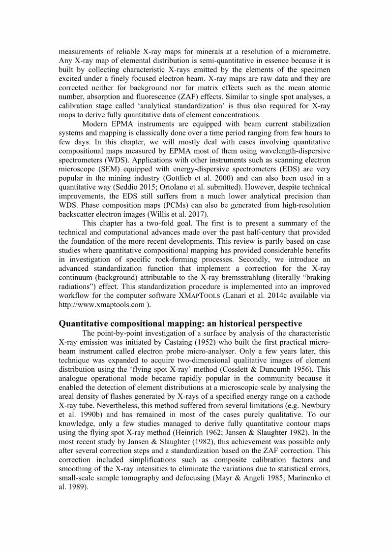
An example of quantitative mapping by EPMA with a typical analytical setup is presented in the following to show some advantages of this approach compared to single-spot analyses. A map of 600 × 520 pixels was generated at the Institute of Geological Sciences of the University of Bern using a JEOL 8200 superprobe instrument, based on two passes (i.e. two map acquisitions). Accelerating voltage was fixed at 15 keV, specimen current at 100 nA, the beam and step sizes at 1µm and the dwell time at 160 ms. This setup enabled to measure nine elements by WDS and seven elements by EDS. The total measurement time for mapping was approximately 30 h corresponding to 15 h per scan (Fig. 1). Note that shorter dwell time may be used to save measurement time but it affects the analytical precision proportionally (see below). In this example, the total measurement time can be reduced to 15 h using dwell time of 80 ms and 7.5 h using dwell time of 40 ms.

The investigated sample is a garnet-bearing metasediment from Val Malone (Southern Sesia Zone, Italian Western Alps) recording blueschist to eclogite facies conditions during the Alpine orogeny (Pognante 1989). To track possible drift in the X-ray production during the time window of the map acquisition, the average and standard deviation (2σ) of the aluminium Kα X-ray counts of every single line scan (corresponding to a single column in the image and an acquisition time of 90 seconds) in the map were plotted against the measurement time (Fig. 1d). Aluminium is expected to be constant in the alpine garnet in the absence of ferric iron (labelled Grt2 in Fig. 1a). It is interesting to note that no significant time-dependent intensity drift was observed during this first pass and thus, the corresponding X-ray maps can be directly transformed into maps of element concentrations using one of the standardization procedures available in the literature (e.g. Cossio & Borghi 1998; Clarke et al. 2001; De Andrade et al. 2006). Acquisition times longer than 30 h may involve a time-dependent drift in the X-ray production caused by small variations of the beam energy in the specimen. In this case, the resulting drift needs to be corrected prior to standardization by flattening the intensity of a phase having a homogeneous composition. Software tools for intensity drift corrections are presented below.

For the current example, the X-ray maps were standardized using spot analyses as internal standards (Fig. 1c) and the software XMAPTOOLS 2.4.1 (Lanari et al. 2014c). The calibrated map contains 312,000 pixels. After the exclusion of the ‘mixed’ pixels occurring at the grain boundaries, ~290,000 spatially resolved fully quantitative analyses were obtained. The average analytical precision for a single garnet pixel composition ranges between 2.8 % for Si and 20 % for Mn (2σ, see Tab. 1). One of the main advantages of the quantitative mapping approach compared to traditional single-spot analyses is that the composition of several pixels of homogenous material can be averaged, significantly increasing the analytical precision and the possibility to detect slight compositional zoning. An averaging over a 10 × 10 µm2 square window as the one plotted in Figure 1a reduces for example the mean analytical uncertainty of garnet composition to 0.28 % for Si and 2 % for Mn. Statistic tools are therefore needed to integrate pixel information along several spatial and compositional dimensions to identify and quantify small amounts of compositional zonation in the analysed sample (Cossio & Borghi 1998; Tinkham & Ghent 2005; Lanari et al. 2014c). The example presented above shows that quantitative X-ray mapping represents an extremely precise analytical technique, opening new prospects for accurate studies of various geological materials.

Fig. 1. Mapping example of a HP mylonite from the Southern Sesia Zone (Western Alps, Italy) and stability test of the mapping conditions in homogeneous material during analysis. (a) Semi-quantitative Al Kα X-ray map. White square (bottom left part of the garnet): example of integration 10 × 10 pixels window (see Tab. 1 and text for details). The Al content in garnet core (Grt1) is lower due to the presence of Fe3+ substituting with Al. (b) Mask image of the mapped sample. White: pixels used for the stability test. The phase boundaries were removed using the BRC correction of XMAPTOOLS to avoid mixed pixels and secondary fluorescence effects. Ion probe spot analyses (SIMS spots in panel a) were manually removed as the topography of the crater affected the measured X-ray intensity because of variable absorption thickness. (c) Calibration curve (dashed line) for garnet Grt2 using the advanced standardization procedure described in this study. The error bars represent the uncertainty on individual pixel composition determined from the counting statistics (at 2σ) using a Poisson law. (d) Test for time-dependent drift in Al Kα X-ray intensity of Grt2 with time. Al is assumed to be constant in Grt2 in the absence of significant variations of XFe3+ (< 0.01 %). The red spots represent the mean value of each pixel column (measured in a time range of ~ 90 seconds) and the vertical bars represent the relative standard deviation (at 2σ). No time-related drift in the measured intensity is observed over 15 hours of acquisition for this map.

Quantitative compositional mapping as a tool to track compositional changes and investigate rock-forming processes

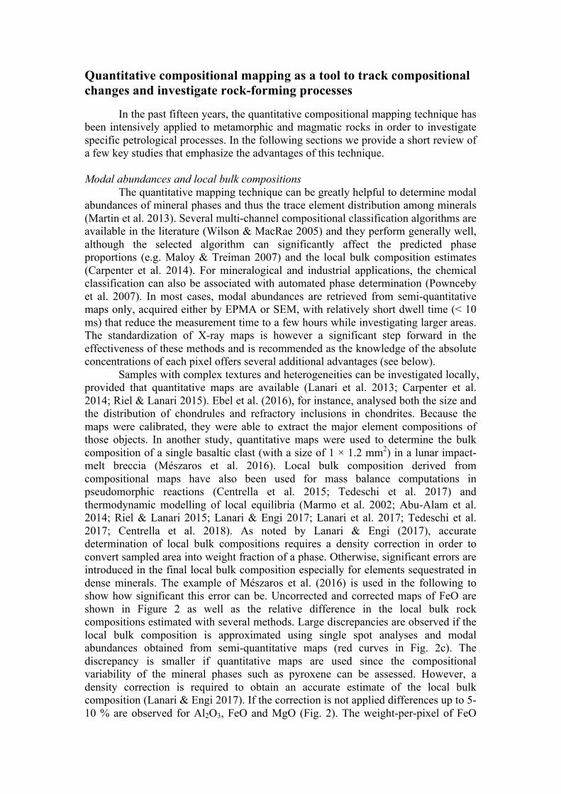
In the past fifteen years, the quantitative compositional mapping technique has been intensively applied to metamorphic and magmatic rocks in order to investigate specific petrological processes. In the following sections we provide a short review of a few key studies that emphasize the advantages of this technique. Modal abundances and local bulk compositions The quantitative mapping technique can be greatly helpful to determine modal abundances of mineral phases and thus the trace element distribution among minerals (Martin et al. 2013). Several multi-channel compositional classification algorithms are available in the literature (Wilson & MacRae 2005) and they perform generally well, although the selected algorithm can significantly affect the predicted phase proportions (e.g. Maloy & Treiman 2007) and the local bulk composition estimates (Carpenter et al. 2014). For mineralogical and industrial applications, the chemical classification can also be associated with automated phase determination (Pownceby et al. 2007). In most cases, modal abundances are retrieved from semi-quantitative maps only, acquired either by EPMA or SEM, with relatively short dwell time (< 10 ms) that reduce the measurement time to a few hours while investigating larger areas. The standardization of X-ray maps is however a significant step forward in the effectiveness of these methods and is recommended as the knowledge of the absolute concentrations of each pixel offers several additional advantages (see below).

Samples with complex textures and heterogeneities can be investigated locally, provided that quantitative maps are available (Lanari et al. 2013; Carpenter et al. 2014; Riel & Lanari 2015). Ebel et al. (2016), for instance, analysed both the size and the distribution of chondrules and refractory inclusions in chondrites. Because the maps were calibrated, they were able to extract the major element compositions of those objects. In another study, quantitative maps were used to determine the bulk composition of a single basaltic clast (with a size of 1 × 1.2 mm2) in a lunar impact-melt breccia (Mészaros et al. 2016). Local bulk composition derived from compositional maps have also been used for mass balance computations in pseudomorphic reactions (Centrella et al. 2015; Tedeschi et al. 2017) and thermodynamic modelling of local equilibria (Marmo et al. 2002; Abu-Alam et al. 2014; Riel & Lanari 2015; Lanari & Engi 2017; Lanari et al. 2017; Tedeschi et al. 2017; Centrella et al. 2018). As noted by Lanari & Engi (2017), accurate determination of local bulk compositions requires a density correction in order to convert sampled area into weight fraction of a phase. Otherwise, significant errors are introduced in the final local bulk composition especially for elements sequestrated in dense minerals. The example of Mészaros et al. (2016) is used in the following to show how significant this error can be. Uncorrected and corrected maps of FeO are shown in Figure 2 as well as the relative difference in the local bulk rock compositions estimated with several methods. Large discrepancies are observed if the local bulk composition is approximated using single spot analyses and modal abundances obtained from semi-quantitative maps (red curves in Fig. 2c). The discrepancy is smaller if quantitative maps are used since the compositional variability of the mineral phases such as pyroxene can be assessed. However, a density correction is required to obtain an accurate estimate of the local bulk composition (Lanari & Engi 2017). If the correction is not applied differences up to 5-10 % are observed for Al2O3, FeO and MgO (Fig. 2). The weight-per-pixel of FeO

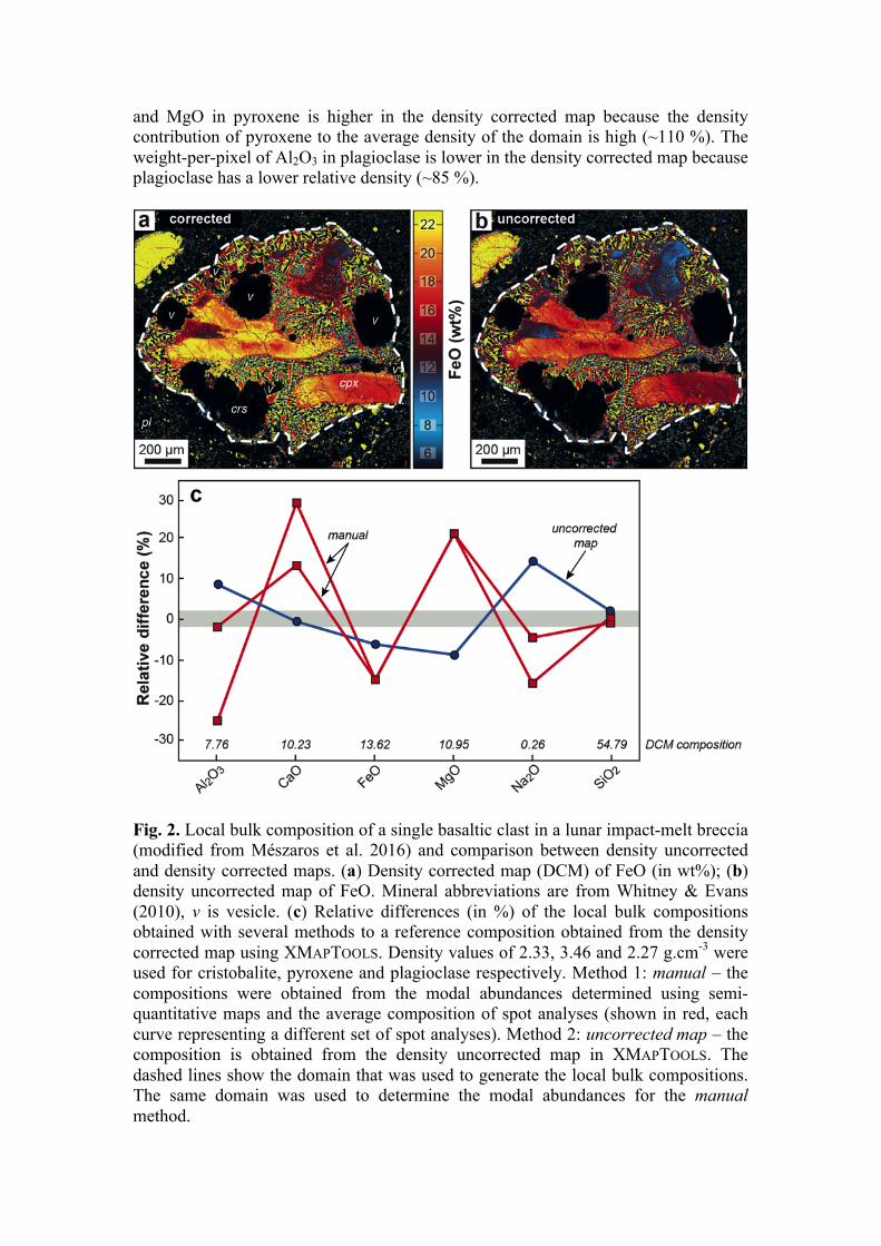
and MgO in pyroxene is higher in the density corrected map because the density contribution of pyroxene to the average density of the domain is high (~110 %). The weight-per-pixel of Al2O3 in plagioclase is lower in the density corrected map because plagioclase has a lower relative density (~85 %).

Fig. 2. Local bulk composition of a single basaltic clast in a lunar impact-melt breccia (modified from Mészaros et al. 2016) and comparison between density uncorrected and density corrected maps. (a) Density corrected map (DCM) of FeO (in wt%); (b) density uncorrected map of FeO. Mineral abbreviations are from Whitney & Evans (2010), v is vesicle. (c) Relative differences (in %) of the local bulk compositions obtained with several methods to a reference composition obtained from the density corrected map using XMAPTOOLS. Density values of 2.33, 3.46 and 2.27 g.cm-3 were used for cristobalite, pyroxene and plagioclase respectively. Method 1: manual – the compositions were obtained from the modal abundances determined using semi-quantitative maps and the average composition of spot analyses (shown in red, each curve representing a different set of spot analyses). Method 2: uncorrected map – the composition is obtained from the density uncorrected map in XMAPTOOLS. The dashed lines show the domain that was used to generate the local bulk compositions. The same domain was used to determine the modal abundances for the manual method.

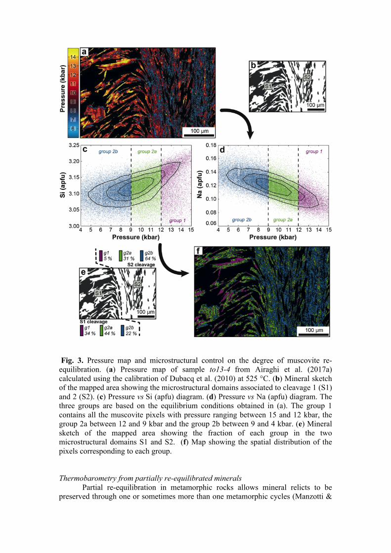
Fig. 3. Pressure map and microstructural control on the degree of muscovite re-equilibration. (a) Pressure map of sample to13-4 from Airaghi et al. (2017a) calculated using the calibration of Dubacq et al. (2010) at 525 °C. (b) Mineral sketch of the mapped area showing the microstructural domains associated to cleavage 1 (S1) and 2 (S2). (c) Pressure vs Si (apfu) diagram. (d) Pressure vs Na (apfu) diagram. The three groups are based on the equilibrium conditions obtained in (a). The group 1 contains all the muscovite pixels with pressure ranging between 15 and 12 kbar, the group 2a between 12 and 9 kbar and the group 2b between 9 and 4 kbar. (e) Mineral sketch of the mapped area showing the fraction of each group in the two microstructural domains S1 and S2. (f) Map showing the spatial distribution of the pixels corresponding to each group. Thermobarometry from partially re-equilibrated minerals

Partial re-equilibration in metamorphic rocks allows mineral relicts to be preserved through one or sometimes more than one metamorphic cycles (Manzotti &

Ballèvre 2013). These relics are important archives for petrologists as they reflect changes in equilibrium conditions and can be used to retrieve individual P-T stages or segments of the P-T paths. Single spot analyses by EPMA are traditionally used to calculate activities of end-members in solid solution and thus to model mineral reactions and mineral stability (see Spear et al. 2016 for a review). Garnet is one of the most famous thermobarometers and numerous calibrations have been derived by the community to evaluate the P-T conditions from garnet compositions either through the equilibrium with another Fe-Mg phase or by using isochemical phase diagrams (Baxter et al. 2017). However, one of the key aspects of garnet thermobarometry is an understanding of the processes that control the local mineral composition during growth (Kohn 2014). Compositional maps may help to clarify whether the observed compositional zoning derives from continuous or discontinuous reactions involving equilibrium or transport controlled growth (Spear & Daniel 2001; Yang & Rivers 2001; Hirsch et al. 2003; Angiboust et al. 2014; Ague & Axler 2016; Lanari & Engi 2017). Empirical and semi-empirical thermometers and barometers are also available for a large spectrum of magmatic and metamorphic mineral phases (for variable bulk rock compositions) and can be easily applied to derive temperature or pressure maps (De Andrade et al. 2006; Lanari et al. 2014c; Lanari et al. 2014a; Trincal et al. 2015). The identification of the compositional variability, not only through the mineral assemblage, but also within a single grain has proven to be a great assistance for thermobarometric studies (Marmo et al. 2002; Lanari et al. 2013; Abu-Alam et al. 2014; Loury et al. 2016). More challenging are the high-variance assemblages involving phyllosilicates forming at lower metamorphic conditions. Originally, their investigation has required a multi-equilibrium approach that relies on complex solid solution models (Vidal & Parra 2000; Vidal et al. 2001; Parra et al. 2002; Parra et al. 2005; Vidal et al. 2006; Dubacq et al. 2010). These techniques had significant successes when applied to compositional maps as the pressure and temperature conditions of formation can be put into a micro textural context (Vidal et al. 2006; Ganne et al. 2012; Lanari et al. 2014b; Trincal et al. 2015; Scheffer et al. 2016). It becomes therefore possible to apply multi-equilibrium thermobarometry to specific mineral phases that are observed in textural equilibrium. The assimilation of the textural equilibrium to the thermodynamic equilibrium can lead to misinterpretation of the textural and compositional relationship (see below).

The investigation of the re-equilibration processes in local mineral assemblage require a forward thermodynamic model (Lanari & Engi 2017). Yet compositional maps have shown that the phyllosilicates in the mineral matrix of metapelite preferentially re-equilibrate in zones of high strain, while they are preserved in zones of low strain such as microfold hinges (Abd Elmola et al. 2017; Airaghi et al. 2017b; Airaghi et al. 2017a). The compositional variability observed within the different microstructural positions and the quantification of the modal abundance of each compositional group have been used to demonstrate that the phyllosilicates partially re-equilibrated during prograde metamorphism through pseudomorphic replacement. This process is mostly controlled by the presence of a metamorphic fluid in the intergranular medium. In a detailed study of muscovite composition in amphibolite facies metapelite, Airaghi et al. (2017a) retrieved the P-T conditions of different muscovite compositional groups observed in different microstructural domains. The example of Airaghi et al. (2017a) is used in the following to show how detailed investigation can be carried out using the quantitative mapping approach. A pressure map (Fig. 3a) has been calculated from the compositional maps of muscovite at a fixed temperature of 525°C using the method of Dubacq et al. (2010) and the program

CHLPHGEQUI 1.5 (Lanari 2012). The pressure condition of each pixel is plotted against P- and T-dependent element such as Si (Fig. 3b) and Na (Fig. 3c) in atom per formulae unit (apfu). Muscovite was classified into three groups: the relics of the HP stage (group 1 in Fig. 3), the phengite re-equilibrated between the pressure peak and the temperature peak (group 2a in Fig. 3), and the muscovite re-equilibrated at the temperature peak (group 2b in Fig. 3). The groups 2a and 2b correspond to the compositional group msB of Airaghi et al. (2017a). Here the distinction is based on the equilibrium conditions rather than on compositional criteria. The main advantage of using compositional maps and chemical diagrams is the ability to depict the spatial distribution of any group of pixels within a given range of composition or equilibrium conditions (Lanari et al. 2014c). The spatial distribution of the three groups of muscovite is shown in Figure 3f. Their relative distribution in both S1 and S2 cleavages can be quantified (Fig. 3e). These results are in line with those of Airaghi et al. (2017a) showing that the metamorphic conditions retrieved for the muscovite groups in different micro-structural positions do not reflect the P-T conditions of the microstructure-forming stages. Rather they document successive fluid-assisted re-equilibration events. Matrix minerals can continue to partially re-equilibrate during prograde metamorphism once the deformation ceased. Similar replacement textures have been also documented in other phases such as chlorite (Lanari et al. 2012), biotite (Airaghi et al. 2017a) and garnet (Martin et al. 2011; Lanari et al. 2017) using quantitative compositional mapping. Petrochronology

The technique of quantitative compositional mapping is extremely helpful in petrochronological studies (see Engi et al. 2017) to link metamorphic stages and reactions to ages retrieved from major and accessory minerals (Williams et al. 2017). In favourable cases, an age map can be constructed and reveals the continuous spatial distribution of ages (Goncalves et al. 2005). Otherwise, quantitative compositional mapping allows the most appropriate spots for dating to be identified. For example, quantitative compositional mapping of allanite may reveal the existence of cores and rims of different composition that, if large enough, could be dated separately (Burn 2016; Engi 2017). The mapping of the compositional heterogeneities in white mica can highlight the most homogeneous grains for the 40Ar/39Ar dating. In addition, it provides a strong petrological basis for interpreting the variability of in-situ Ar 40Ar/39Ar dates (Airaghi et al. 2017b). The spatial resolution is often lower than the characteristic size of the compositional variations in mica (Cossette et al. 2015; Berger et al. 2017; Laurent 2017).

To conclude this short overview we can state that quantitative mapping is therefore becoming an essential tool to provide a comprehensive image of the petrological, thermobarometric and geochronological evolution of metamorphic rocks. Standardization techniques: advantages and pitfalls

The extraction of elemental concentration values from X-ray intensities requires matrix and other corrections. The X-ray data need to be standardized post-collection either relative to similar data collected on natural and synthetic standards using an empirical correction scheme (Jansen & Slaughter 1982; Newbury et al. 1990a, b; Cossio & Borghi 1998; Clarke et al. 2001; Chouinard & Donovan 2015) or against internal standards assuming no matrix effects (De Andrade et al. 2006). Those techniques are separately described in the following.

Castaing’s first approximation to quantitative analysis and matrix effects As first noted by Castaing (1952), the primary generated X-ray intensities are

proportional to the respective weight concentration of the corresponding elements in the specimen. In absence of significant matrix differences between unknown and standard materials, this assumption can be expressed as:

𝐶!!"#

𝐶!!"#≈𝐼!!"#

𝐼!!"# (1)

where the terms 𝐶!!"# and 𝐶!!"# are the composition expressed in weight concentration of the element i in the unknown and the standard and the terms 𝐼!!"# and 𝐼!!"# represent the net corresponding X-ray intensities corrected for continuum background (see below) and any possible other issues such as peak overlap or drift. In the case of significant physical and/or chemical differences between the unknown and the standard (i.e. matrix effects), the Equation (1) becomes:

𝐶!!"#

𝐶!!"#= 𝑘!

𝐼!!"#

𝐼!!"# (2)

where k represents a correction coefficient expressing the non-linear matrix effects. In the specialized literature these effects are divided into atomic number (Zi), X-ray absorption (Ai) and X-ray fluorescence (Fi) effects. The correction must be applied separately for each element present in both the analysed specimen and in a given standard reference material. Bence-Albee empirical correction The empirical procedure of Bence & Albee (1968) is based upon known binary experimental data and it involves less computation time than the ZAF correction described in the following. It assumes a simple hyperbolic calibration curve between the weight concentrations and the net intensities of a given oxide in binary system (Ziebold & Ogilvie 1964). The calibration curve is described in terms of a single conversion parameter known as the α-factor

1− 𝐼!𝐼!

= 𝛼!"1− 𝐶!𝐶!

(3)

with 𝛼!" the α-factor for a binary between elements A and B; IA and Ca the net intensity and mass concentration, respectively. This approach has been generalized by Bence & Albee (1968) to more complicated oxide systems of n components using a linear combination of α-factors such that:

𝐶!𝐼!=𝑘!𝛼!! + 𝑘!𝛼!! +⋯+ 𝑘!𝛼!!

𝑘! + 𝑘! +⋯+ 𝑘! (4)

where 𝛼!! is the α-factor for the n1 binary used to determine the concentration of element n in a binary between n and 1. Clarke et al. (2001) applied this procedure to standardize X-ray maps into map of oxide mass concentrations. Several tests have indeed shown that the Bence & Albee (1968) procedure yields results comparable to those obtained with the ZAF method (Goldstein et al. 2003) while reducing significantly the computation time for corrections (Clarke et al. 2001). The accuracy of this method mostly depends on the quality of the α-factor estimates, as well as the choice of homogeneous and well-characterized standard materials. Most of the correction factors for oxides and silicates are well constrained and updates including small improvements are regularly published (Albee & Ray 1970; Love & Scott 1978; Armstrong 1984; Kato 2005). The

software XRMAPANAL (Tinkham & Ghent 2005) uses the Bence-Albee algorithm to standardize X-ray maps and provides several tools to display maps, compositional graphs and to perform advanced statistical analyses. ZAF and ϕ(ρz) corrections The ZAF matrix correction was the first generalized algebraic procedure. This standardization method is based on a more rigorous physical model taking into account the atomic number effects, the absorption and fluorescence in the specimen. The ratio of concentration in unknown and standard of an element i is given by

𝐶!!"#

𝐶!!"#= 𝑍𝐴𝐹 !

𝐼!!"#

𝐼!!"# (5)

where 𝑍𝐴𝐹 ! is the ZAF correction coefficient. Typical values of the ZAF coefficient for metals are reported in several text books (e.g. Goldstein et al. 2003; Reed 2005).

The direct calculation of absorption in the original ZAF correction scheme was lately improved by introducing an empirical expression of ϕ(ρz) to correct for absorption (Packwood & Brown 1981). In the mid-80’s several ϕ(ρz) algorithms (e.g. Riveros et al. 1992) including more accurate sets of mass absorption coefficients were successively developed: PROZA (Bastin et al. 1986), citiZAF (Armstrong 1988), PAP (Pouchou & Pichoir 1991), XPhi (Merlet 1994). Some of them are still used in modern EPMA instruments. It is crucial for the ZAF or ϕ(ρz) corrections to measure all the major and minor elements present in the specimen to ensure that all the possible matrix effects are taken into account. Both ZAF and ϕ(ρz) correction algorithms have been applied to X-ray maps in order to generate maps of oxide mass concentrations (Jansen & Slaughter 1982; Cossio & Borghi 1998; Prêt et al. 2010) and this option is currently available in the software PETROMAP (Cossio & Borghi 1998) and in CAMECA’s commercial software provided with the SX100. There are two main limits of this technique. First, it is necessary to perform an accurate background correction to the X-ray maps prior to standardization. This correction requires either the acquisition of upper and lower peak background maps or the use of models to predict the theoretical background values (e.g. Tinkham & Ghent 2005). The MAN algorithm for instance allows the background value to be predicted from the mean atomic number of the specimen (Donovan & Tingle 2003; Chouinard & Donovan 2015; Wark & Donovan 2017), significantly reducing the total acquisition time. The second limitation is the large relative uncertainty in the intensity of each pixel (see Tab. 1). This uncertainty is propagated through the ZAF factors. To overcome this issue, Jansen & Slaughter (1982) applied a preliminary ZAF correction to a group of pixels of the same mineral phase in order to derive an estimate of the ZAF correction factors yielding for this phase. These factors are then used to correct compositionally similar pixels. This option is not available to our knowledge in any commercial software or freeware solution. Internal standardization using high-precision spot analyses

Of primary importance in routine EPMA analyses, are the analytical precision and accuracy of spot analyses. The quality of standardization in spot analysis can be quickly evaluated using either a reference material with known concentration, or stoichiometric constraints on unknown mineral phases. These tests are routinely applied before each analytical session and ensure the high quality of the data produced. The internal standardization procedure of X-ray maps takes advantage of

the excellent quality of spot analyses. The goal is to calibrate the X-ray maps of every mineral phase using high precision spot analyses of the same mineral phase (Mayr & Angeli 1985; De Andrade et al. 2006). In this case, there are no matrix effects between the unknowns (X-ray maps) and the standards (spot analyses):

𝐶!!"# =!!!"#

!!!"# 𝐼!!"#

∗ + 𝐼!!"#$ (6)

with 𝐼!!"#∗ the X-ray intensity of the unknown uncorrected for background and 𝐼!!"#$

the intensity of background. This approach results in a strong dependence of the accuracy of the compositional maps upon the accuracy of the spot analyses selected for the standardization. The internal standardization procedure has been implemented in a MATLAB©-based computer program (De Andrade et al. 2006), in the software solutions XMAPTOOLS (Lanari et al. 2014c) and QNTMAP (Yasumoto et al. submitted). Spatial and chemical resolution and possible issues Spatial resolution

In compositional mapping, the spatial resolution is determined by the spacing of spot measurements and the X-ray excitation volume of the electron beam. It is recommended to use a beam size smaller than the pixel size to reduce overlapping (see XMAPTOOLS’ user guide for examples). For a given spacing between two pixels, an increasing beam size will increase the fraction of ‘mixed’ pixels (i.e. mixed phases see below).

Chemical resolution

The chemical resolution of an individual pixel depends on the dwell time, the accelerating voltage and the beam current. The relative precision of any measurement can be estimated using counting statistics (the generation of characteristic X-rays is a Poisson process) from the total number of X-rays collected by the detector. Examples of analytical precisions for different elements are given in Table 1.

As shown in the introduction, as soon as several pixels are taken into account, the relative uncertainty and detection limits decrease relative to the values obtained by single pixel counting statistics. Averaging of pixels of unzoned material or of a single growth zone virtually increases the counting time thus reducing the relative uncertainty (Tab. 1). This effect applies to any map, as the human eye is an outstanding integrator of visual information as the human brain is able to detect gradients even in noisy signals. If a mineral phase extends over a substantial lateral range of pixels, it might be possible to discern compositional zoning below the detection limit despite the noise that results from statistical fluctuations in the count at a single pixel (Newbury et al. 1990a; Friel & Lyman 2006). Issues

Radiation damage. Some elements, and particularly light elements, are affected by degradation induced by local heating effects from electron beam exposure over time. Either an increase or decrease in intensity could be observed because of radiation damage. A decrease in intensity may reflect a loss of mass by volatilization. The low-energy X-rays of volatile elements undergo a strong self-absorption in the specimen that increases if the beam energy is increased (Goldstein et al. 2003). Therefore, light elements (Na. K, Ca) have to be measured with the lowest beam energy possible, during the first pass of the beam over the mapped area

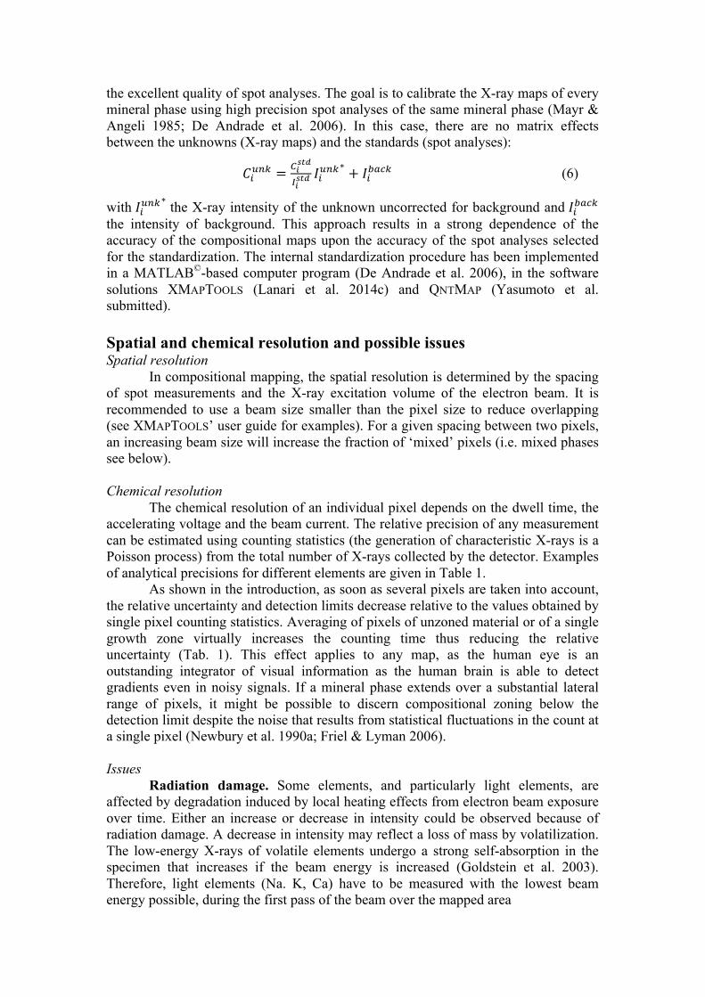
Fig. 4. Examples of apparent compositional zoning in quartz caused by secondary fluorescence effects. The scale bars show number of recorded X-ray counts. Mineral abbreviations are from Whitney & Evans (2010). Mixed pixels have been removed using the BRC correction (see text). The phases shown in white do not play any role for secondary fluorescence effects. (a) Map of a micaschist sample from The Briançonnais Zone (Chaberton Area) in the Western Alps (Verly 2014) showing the secondary fluorescence of Fe in quartz at the contact with chlorite (light grey) but not with phengite (dark grey). White: plagioclase and rutile. (b) Map of a mafic eclogite from the Stak massif in NW Himalaya (Lanari et al. 2013; Lanari et al. 2014c). An apparent zoning in Ti is observed in clinopyroxene (area 1) at the contact with rutile, caused by secondary fluorescence of Ti, while a ‘real’ compositional zoning of Ti is present in clinopyroxene and correlated with the variations in other major element concentrations (area 2). White: garnet, amphibole, plagioclase and Fe-oxide. (c) Map of a schist belonging to the TGU (Theodul Gletscher Unit) in the Zermatt area. Secondary fluorescence of Ca observed in quartz at the contact with garnet (dark grey) and plagioclase (light grey). White: rutile, titanite, apatite, phengite, paragonite, pyrite, zoisite and epidote. (d) Secondary fluorescence of Fe in quartz at the contact with garnet (light grey) and chlorite (dark grey) in another schist from the TGU. White: paragonite, phengite, albite, pyrite, chlorite, zoisite, rutile, titanite and apatite.

Secondary fluorescence effects. A secondary fluoresce effect occurs when

the characteristic X-rays of a given element generate a secondary generation of characteristic X-ray of another element. Because X-rays penetrate into matter farther than electrons, the interacting volume of X-ray-induced fluorescence is generally greater (up to 99% larger as proposed by Goldstein et al. 2003). This volume may

include more than one phase, and the induced X-rays originate from different contributions. In X-ray images, secondary fluorescence effects can occur near phase boundaries (e.g. Fig. 4) or melt inclusions (Chouinard et al. 2014). Compositional mapping is a powerful tool to detect potential effects of secondary fluorescence that would not be seen otherwise. Figure 4 shows a few examples involving an apparent compositional zoning that is caused by secondary fluorescence effects. Secondary fluorescence can affect several elements and is commonly associated with the presence of anorthite (Ca), chlorite (Fe), epidote (Fe), garnet (Ca) or rutile (Ti). One of the best candidates in which to observe secondary fluorescence effects is quartz (Fig. 4a,c-d). The X-ray intensity caused by secondary fluorescence in a surrounding mineral decreases from the source toward the inner part with a distance up to 100 µm at 15 keV, 100 nA and for counting time < 300 ms (Fig. 4). Particular attention must be paid when comparing differences of minor to trace elements concentrations in phases occurring both as inclusions in a porphyroblasts and within the mineral matrix. In the example shown in Figure 4d, quartz exhibits higher count rates of Ca in the grains trapped as inclusions in garnet compared to those in the matrix. Note that a slight secondary effect is also observed in the pressure shadows of garnet where chlorite is present (light grey in Fig. 4d). If a mineral with low Ca, Fe and Ti concentrations displays higher concentrations in a porphyroblast showing high Ca, Fe and Ti contents, one might suspect a secondary fluorescence effect. In quartz inclusions FeO can be overestimated by 0.25 to 0.65 wt% (Fig. 4d).

Thermal instability of the instrument. Several parts of the EPMA instrument are sensitive to temperature changes. The gas commonly used as ionization medium to produce a secondary cascade of electrons amplifying the signal in the proportional counter, must have a constant pressure over time in order to ensure the reproducibility in counting rates between the standards and the unknown. The spectrometer crystals are also affected by thermal expansion, yielding to a change in the Bragg angle and a consequent shift in the peak position (Jenkins & De Vries 1982; Delgado-Aparicio et al. 2013).

Beam current stability. For any kind of quantitative analyses, the quality of the data depends also strongly on beam current stability. The adjustment of the balance between beam accelerating voltage and beam current allows the analytical setup between spatial resolution and sensitivity to be optimized. Higher beam energies results in higher count rates, but with a significant loss of spatial resolution due to the greater interaction volume (e.g. Hombourger & Outrequin 2013 for field emission EPMA). A variation in the beam energy during mapping causes an apparent variation of the number of characteristic X-rays produced in the specimen. This issue is visible if the element intensity shows a linear evolution with time of in a homogeneous mineral phase.

Spectrometer focus. In a fully focused WD spectrometer, the electron beam, the specimen, the analysing crystal and the detector are all located on constrained geometry to satisfy the Bragg condition for the desired wavelength. This geometry brings all the X-rays originating from the source to be focused at the same point on the detector, and maximizes the collected radiation (Goldstein et al. 2003). During WDS mapping with fixed stage and scanning beam, the beam may be scanned off the point of optimum focus and the X-ray intensity decreases as a function of the deflection (Newbury et al. 1990b). An example showing how spectrometer defocusing during mapping can affect the X-ray counting rate is presented below in the section

Corrections Surface irregularities. The presence of topography at the specimen surface

affects the measurements during X-ray mapping. The beam converges on the plan of optimum focus, but it broadens above and below it. When the specimen surface is not flat, different beam volumes may analyse different specimen portions. These features will not appear in focus and will cause a decrease of intensity as discussed above. The local topography affects the angle of incidence between the beam and the specimen surface, and hence the number and trajectories of measured BSE and SE of the backscattered electrons depends on the local orientation. The deviation from the ideal angle results in a backscattered electron distribution distorted with the peak and so a decrease in intensity. A complex surface also affects the local thickness of sample along the X-ray path toward the detector. This effect is known as the geometric absorption effect (Goldstein et al. 2003).

Quantitative mapping procedure

The procedure for obtaining compositional maps of elemental concentrations of a micrometre- to millimetre-sized domain involves several steps:

1. Define the problem: what do we want to learn from this map? As for traditional spot analyses, this decision will define the analysis procedures (see Goldstein et al. 2003 for a complete description). For compositional mapping, the analytical procedure used to investigate the compositional zoning of a millimetre-sized porphyroblast (high chemical resolution but low ability to identify small phases) is for example different from the one that will be used to estimate a local bulk composition (higher ability to identify small phases but lower chemical resolution).

2. Sample characterization using the optical microscope or SEM – including BSE and EDS qualitative analyses – to determine the mineral phases to be investigated. It is critical to know prior each mapping session the size of the smallest object to be analysed. The spatial resolution of the map, corresponding to the step size, must be at least five to ten times smaller to identify possible compositional zoning within single grains. It is important to distinguish between ‘pure’ pixels recorded away from grain boundaries and ‘mixed’ pixels recording mixing information (Launeau et al. 1994). Only pure pixels can be used directly to measure the compositional variability of a given mineral phase. It is important to minimize as much as possible the presence of mixed pixels in the maps by using small beam size (< 1µm for the map acquisition), as mixed pixels are the main source of misclassification (Maloy & Treiman 2007). Small spot sizes also reduce the need of density correction if several phases are measured in a single pixel (Ebel et al. 2016).

3. Select the sample and the appropriate area to be investigated. The surface of the mapped area together with the step-size and the number of elements measured by WDS determines the total measurement time to be added to the time for the acquisition of point analyses necessary for the map standardization.

4. Measure the spot analyses that will be used as internal standards for X-ray map standardization. This step requires the calibration of the spot analyses using either the ZAF or ϕ(ρz) corrections and appropriate standard materials. We recommend measurement of at least one horizontal and one vertical transect starting and ending at grain boundaries that can be easily recognized

on the final X-ray maps. This will permit to detect and correct potential shifts in the position of the spot analyses relative to the map (see below). The distance between two spot analyses along a given transect must be a factor of the pixel size (step-size) to avoid additional uncertainties introduced during the projection. Additional spot analyses can be defined using BSE images. We recommend measuring between 10 and 20 spot analyses per phases to be standardized. This is particularly critical for mineral phases exhibiting compositional zoning. Phases with known composition can be standardized using a fixed composition (e.g. 100 wt% of SiO2 for quartz).

5. Check the quality of the spot analyses. As discussed above, the accuracy of the standardized maps depends mostly on the accuracy of the spot analyses to be used as internal standards. It is thus critical to evaluate the quality of the spot analyses using the concentrations expressed in oxide weight percentage and the structural formulas.

6. Collect the X-ray maps using WDS or/and EDS and the TOPO, SEI and/or BSE images.

7. Export the X-ray maps as matrixes containing raw X-ray counts. It is not recommended to use pseudo-coloured images exported by the instrument software.

An advanced standardization procedure implemented in XMAPTOOLS’ workflow

A description of the different steps of data processing is given in the following sections. Multi-channel compositional classification

The multi-channel compositional classification process allows the pixels of X-ray maps to be categorized according to chemical information contained in the element X-ray intensities. Several algorithms are available in the literature (Wilson & MacRae 2005) and implemented in the available software solutions (Cossio & Borghi 1998; Clarke et al. 2001; Tinkham & Ghent 2005; Ortolano et al. 2014; Yasumoto et al. submitted). In XMAPTOOLS the automated classification procedure is based upon the k-means algorithm and requires the manual sampling of a representing pixel for each previously identified phase (Lanari et al. 2014c). The function generates a mask file containing the distribution of each mineral phase defined by the user. A mask file can also be generated manually by selecting different groups of pixels out of binary or a ternary chemical plots or by combining mask files from different classifications. Once a mask file is generated, it may be merged with another mask file, or the group may be further split by manual selection on chemical plots. Corrections

If needed, corrections to the raw X-ray maps can be applied right after the multi-channel compositional classification. Corrections include dead time correction for WDS, intensity drift or topography corrections as well as the adjustment of the map and/or standard positions.

Dead time correction (WDS). During EMPA analyses performed with WDS, each pulse arriving from the detector is being processed by the electronics. In the meanwhile, the detector remains completely blind to any incoming X-ray photon for a

time interval defined as ‘dead time’. A dead time correction has therefore to be applied to the effective analytical counting time. In XMAPTOOLS, the dead time correction is applied to X-ray maps measured by WDS using the following relationships:

𝐼!∗ = !!!!! × !"!! × !!

(7)

where 𝐼! and 𝐼!∗ are the measured and dead time corrected count rates of element i (in counts per second) and 𝜏 the characteristic dead time of the detector in seconds.

Sample surface topography. Sample topography such as holes or irregular surfaces may have a significant effect on the produced X-ray intensities. The local topography introduces variable absorption path-length in different directions, so that the intensity emitted varies according to the spectrometer position (Newbury et al. 1990a). A TOPO map can be measured in JEOL EPMA instruments using the Solid State BSE detector. This detector consists of two opposite segments: one located at the top of the image field and one located at the bottom. The topographic image is constructed from the difference between the BSE signals returned by the two detectors. The topography image corresponds to a light illumination at oblique incidence and suppresses the atomic number contrast component of the BSE signal (Kässens & Reimer 1996). In the XMAPTOOLS software, the topography correction can be applied using the TRC module (TRC is for TOPO-related correction) when a correlation is observed between the X-ray intensities of an element in a given phase and the intensity of the TOPO map. The magnitude of the correction depends on the spectrometer used, the element and the mineral phase analysed as the absorption changes with the position of the spectrometer and the density of the target material.

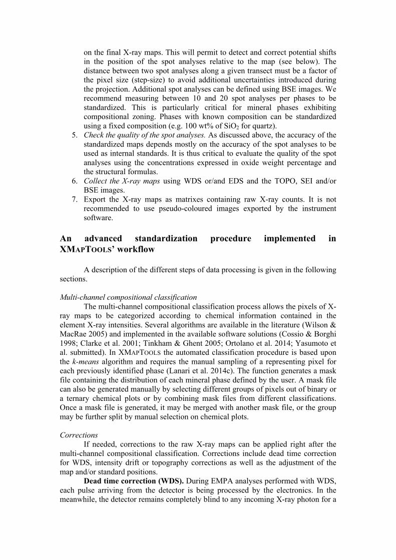
Time-dependent drift. A time-dependent drift in the X-ray production related to small variations of the beam current at the specimen surface may be observed for acquisition periods exceeding 24 h (Fig. 5). There are three major causes for time-dependent drift of the X-ray intensities to occur. First, the probe current can drift during the analysis (e.g. Cossio & Borghi 1998). Second, the vacuum conditions in the gun or the specimen chamber can change with time, causing more (or less) interactions between the electron beam and the gas particles thus decreasing (or increasing) the specimen energy and the production rate of characteristic X-rays. For instance an abrupt increase of the pressure in the gun chamber may cause a sharp decrease in the measured X-ray intensities. The third cause of time-dependent drift may be related to beam-defocusing issues during scanning on a non-flat surface. Defocusing indeed affects the geometry and size of the interaction volume thus affecting the specimen energy density where the characteristic X-rays are produced. The resulting drift might be corrected prior to standardization regardless of the cause of the variation as soon as the time-dependency can be retrieved. For the correction to be performed, a phase equally distributed within the mapped area and showing a homogeneous composition in a given element must be identified. The Intensity Drift Correction (IDC) tool has been implemented in XMAPTOOLS 2.4.1 for this purpose. It enables detection of time-dependent drifts and applies any correction function defined by the user. An example of time-dependent drift observed in a map acquired over ~90 h is presented in Figure 5. The investigated sample is the same as the one described in the introduction (garnet-bearing metasediment from the Southern Sesia Zone in the Western Alps). The Si Kα X-ray map (measured during the first pass) and Al Kα X-ray map (measured during the second pass) of alpine garnet Grt2 were used to track possible time-dependent drift and to define a correction function (Fig. 5). In this

example, the observed time-dependent drift exhibits a constant slope over the whole acquisition time corresponding to an average drift in the X-ray intensities of ~0.02 % per hour (~1 % for each scan of ~45 h). The similarity of the drift in the two scans suggests that it reflects a progressive defocusing of the beam caused by a slight inclination of the sample. This example shows that the beam stabilization system of the JEOL 8200 superprobe used in this study performs well compared to the probe current drift of 0.36 % per hour reported in Cossio & Borghi (1998). However, other maps have shown significant time-dependent drift caused by either vacuum failure in the gun chamber or electron beam current drift. In this case it is vitally important to detect such a drift and to apply the appropriate correction to the X-ray maps prior standardization.

Fig. 5. Example of time-dependent drift for a total measurement time of 90 hours on the sample described in Figure 1. (a, b) Evolution of Si Kα X-ray intensity and Al Kα X-ray intensities in Grt2 with time. Red spots: mean values of each pixel column (corresponding to time interval of ~ 160 seconds). Vertical bars: standard deviation (at 2σ). The observed time-dependent drift is fitted using linear function (blue dashed line). It is interesting to note that the slope of this function remains constant during the whole acquisition time (two passes). (c) Mask image of the mapped area showing in white the pixels used for the stability test. The phase boundaries were removed using the BRC correction. (d, e) Matrixes of correction factors (in %) used to correct the X-ray maps of Si Kα and Al Kα respectively. In both cases, the drift correction is lower than 1%.

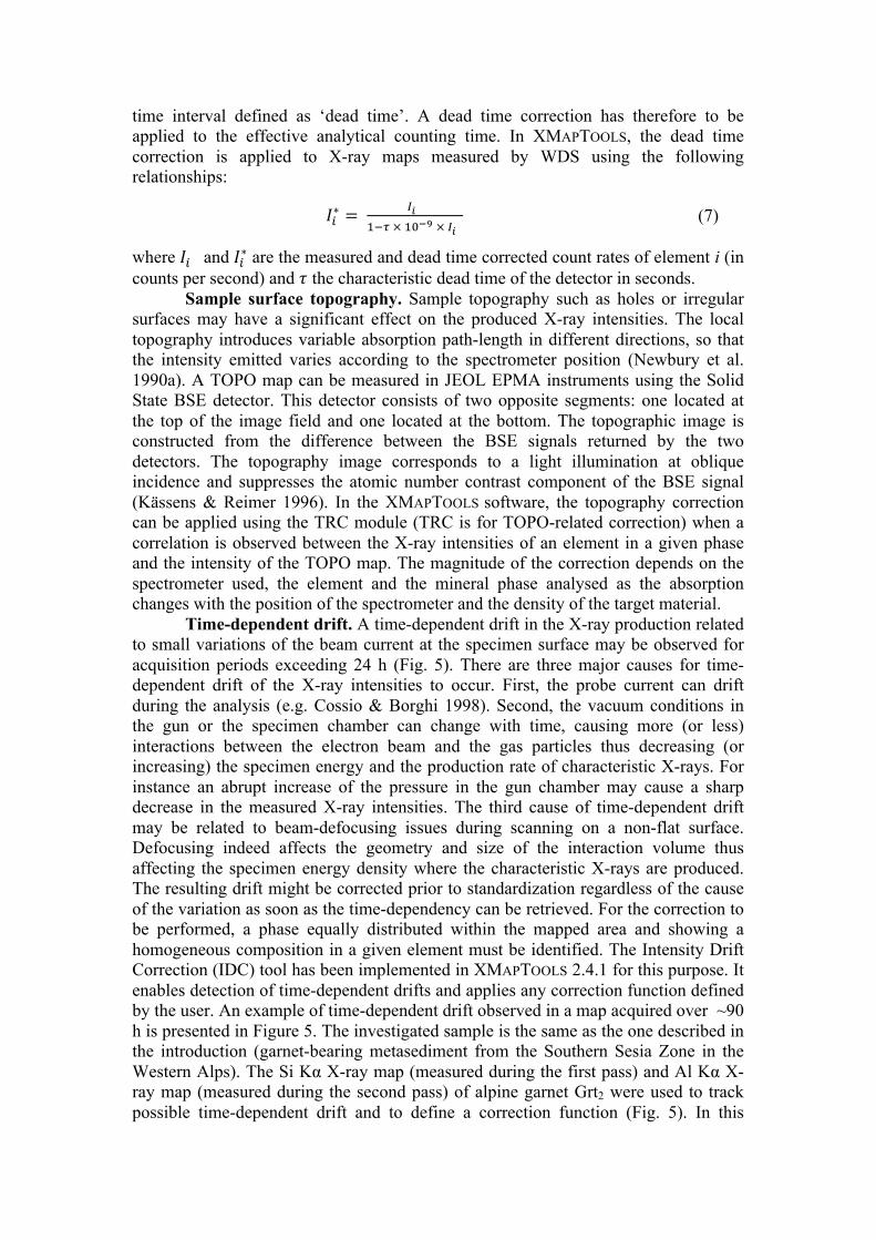
Fig. 6. Positions of spot analyses (internal standard) for the map shown in Figure 5 are tested and corrected using the SPC module of XMAPTOOLS. (a) Case 1: X-ray intensity signal of the Al Kα map pixels corresponding to the original position of the spot analyses obtained from the EPMA coordinates. (b) Al2O3 mass concentration of the spot analyses (internal standards). This trend is used as a reference to evaluate the quality of the projection. The red arrows mark the pixels showing a poor match with (a). (c) X-ray intensity signal of the Al Kα map pixels corresponding to the corrected position of the spot analyses. (d) Synthetic map of the quality of the projection for Case 1. The best position of the spot analyses (internal standard) on the map is calculated as described in the text. In this example, the correlation coefficients were calculated for a 21 × 21 pixels window centred on the original position (white star). The original position is shifted from the optimal position and may be corrected by moving the internal standard position on the map. (e) Synthetic map of the quality of the projection for Case 2. After the correction, the position (black star) corresponds with the best match. It is interesting to notice that even a shift of 2 µm can significantly affect the quality of the match and thus of the standardization.

Mixed pixels and BRC correction. Mixed pixels are commonly observed at the boundary between two phases, depending on the map resolution and beam size (see XMAPTOOLS’ user guide for examples). Resulting localized features do not represent authentic mineral zoning. Mixed pixels can be filtered using the BRC correction (for border-removing correction) available in XMAPTOOLS. This correction removes the pixels located between the different masks of the selected mask file. The correction may be applied for different sizes of the mixing zone depending on the map resolution. An alternative strategy is to evaluate the proportion of phases in each mixed pixel using a distribution-based cluster analysis (Yasumoto et al. submitted).

Fig. 7. Advanced standardization technique based on internal standards. (a) The calibration curve for a given element in a mineral phase is defined using the ranges in oxide mass concentration (ΔC) and in the X-ray intensity (ΔI). The intercept values define the background correction to be applied to the phase of interest. (b) Internal standardization of homogeneous phase (case 1) or of an element below the detection limit in mapping conditions (case 2). (c) Evolution of the difference between standardizations with and without background correction with the oxide mass concentration. (d) Matrix effects in a single mineral (here garnet) causing changes in the slope of the calibration curve.

Maps and standards position. Before performing the analytical standardization, the position of the maps and the spot analyses must be tested and, if necessary, modified based on statistical criteria. It is critical to guaranty that the positions of the spot analyses used as internal standard are not shifted, i.e. that the analysed volume is the same in both analyses. In order to detect such a shift, the standard data (spot analyses, in wt%) can be compared with the intensity data (in counts) of the corresponding pixels on the map, as shown in Figure 6. An algorithm

that detects the optimal position of the maps and the spot analyses is available in XMAPTOOLS. A map of the correlation coefficients between the standard and the intensity data for different X and Y positions is calculated for each element. All maps are then combined to produce a synthetic map evaluating the overall quality of the projection. Examples of good and bad position of standards are shown in Figure 6. In the first case (Case 1 in Fig. 6a,b), the comparison reveals a shift in the position of the spot analyses, corrected using the Standard Position Correction (SPC) tool by shifting vertically the positions of the spot analyses by of 2 µm. In the second case, the quality of the projection was recalculated after correction (Fig. 6d,e). The match between standard values (in wt%, Fig. 6c) and the pixel intensity (in counts, Fig. 4D) is greatly improved. The projection in Case 2 plots in the optimal quality field of the resulting synthetic map. Considering that a shift of few pixels can affect the quality of the match (i.e. in the example in Fig. 4, a shift of 2 µm decreases the quality of the projection by ~ 20%), the standard position correction is crucial to obtain a reliable standardization

Fig. 8. Example of standardization of garnet for Al, Mn and Mg. (a-c) Compositional diagrams showing the compositional ranges observed in the garnet pixels of the X-ray maps (histograms), the internal standards (white dots) with 2σ uncertainty and the calibration curves. The continuous lines are the calibration curves assuming no background, the dashed lines are the calibration curves of the advanced standardization method involving a pseudo-background correction. (d-g) Calibrated maps of MnO and MgO without background correction (d, f) and with background correction (e, g). The colour scales is identical for both images of the same element. (h-i) Difference maps in weight percentage.

Advanced procedure for internal standardization In the XMAPTOOLS software, the analytical standardization is performed using

high-precision spot analyses as internal standards (Lanari et al. 2014c) to obtain numerical concentrations. To be accurate, the X-ray maps need to be corrected for background (see Equation 6) prior to standardization. The background correction is usually applied by using background values of the spot analyses (De Andrade et al. 2006). However it is not applicable if the map and spot analyses are acquired with different spectrometer configurations. For high intensity-to-background ratios, where !!

!!∗!!!

> 20, the background correction is not applied. The spot analyses are indeed

already corrected for background and the map background effects on the calibration curve are negligible. On the contrary, for elements with low intensity-to-background ratios, the background significantly affects the slope of the calibration curve and a background correction is required (see below). The acquisition of lower and upper background maps would triple the measurement time. Hence, an advanced standardization and correction strategy has been implemented to overcome this problem and is described in the following. This calibration does not require any background measurements and is thus extremely powerful at low count rates where the background correction is critical and not always accurately predicted by MAN models (see Fig. 1 in Wark & Donovan 2017).

The advanced standardization technique implemented in XMAPTOOLS 2.4.1 uses the variability commonly observed in the mass concentrations of the standards (ΔC in Fig. 7a) to fit the slope of the calibration curve and to approximate the corresponding background (Equation 6, see the star in Fig. 7a). For this approximation to be accurate, the spot analyses need to capture the majority of the compositional variability of the (zoned) minerals. This pseudo-background correction is not applied to homogeneous phases where ΔC is small (case 1 in Fig. 7b). For trace elements, the compositional variability can be only captured by the spot analyses (case 2 in Fig. 7d), showing that the measured element is below the detection limit for the mapping conditions (Lanari et al. 2014c). As previously mentioned, the difference between a calibration using a background correction and a calibration assuming a fixed background value of zero decreases with increasing intensity-to-background ratios (Fig 7c). It is also important to notice that this advanced technique can only be applied in absence of significant matrix effects in the mineral phase. Matrix effects generally occur if a strong compositional zoning is observed between the core and the rim of a dense mineral such as garnet. In this case, it may be necessary to apply several distinct standardizations one for each garnet composition (Fig. 7d). The matrix differences affect the slopes of the calibration curves (e.g. Lanari et al. 2014c) by underestimating the background value (see the continuous line in Fig. 7d).

An example of garnet standardization is given in Figure 8. The investigated sample is a garnet, kyanite and staurolite bearing metasediment from the Central Alps (Todd & Engi 1997). A millimetre size garnet crystal has been compositionally mapped at the Institute of Geological Sciences of the University of Bern using a JEOL 8200 superprobe instrument. Accelerating voltage was fixed at 15 keV, specimen current at 100 nA, the beam and step sizes at 6 µm and the dwell time at 100 ms. The compositions of garnet core (MnO > 1 wt%) and rims (MnO < 0.7 wt%) are reported in Table 2. The standardization of aluminium does not require any background correction (Fig. 8a), as the intensity-to-background ratio is typically higher than 60 for almandine-rich garnet. The intensity-to-background ratios are much smaller for Mn and Mg (~3 for both cases) and thus a background correction is required. For both

elements the background values have been approximated using the technique presented above (see results in Figs. 8b,c). In this example the spot analyses captured a large range of the observed compositional variability in Mn and Mg. The absence of background correction (continuous lines in Figs. 8b,c) significantly affect the standardize maps with relative differences up to 17 % in MnO and 27 % in MgO (Figs. 8d-g).

Fig. 9. Examples of standardization of garnet and phengite for elements where background corrections are required. The blue rectangles show the reference background values extracted from the background map (see text). The red spots show outliers automatically rejected during the advanced standardization. (a) Mg in garnet. (b) Mn in garnet. (c) Mg in phengite. (d) Na in phengite. (e) Ti in phengite. The symbols are defined in the figure caption of Figure 6.

To evaluate the reliability of this advanced standardization technique and especially the validity of the background predictions, a phengite, chlorite garnet-bearing metasediment from the Zermatt-Saas Zone has been compositionally mapped at the Institute of Geological Sciences of the University of Bern using a JEOL 8200 superprobe instrument with six separate acquisitions of the same map area, two for the peak measurements and four for the off-peak background measurements. Background maps have been calculated assuming a linear background distribution between the lower and upper background values. The measured background values have been compared with the predicted ones for garnet (Mg, Mn, see Fig. 9a,b) and phengite (Mg, Na, Ti see Fig. 9c-e). The predicted and measured background values are in line within 2σ uncertainty for all the elements above detection limits for the mapping conditions and with low intensity-to-background ratios (see Fig. 10). The measured

background values for Mn, Mg, Ca and Ti were also compared with the X-ray intensities measured in quartz. This test shows that the background maps were correctly measured off-peak and that the background values reflect only the contribution of the X-ray bremsstrahlung. To conclude, the advanced standardization technique provided in XMAPTOOLS can successful correct the X-ray maps for background during the standardization. Local bulk compositions, structural formulas and P-T maps The standardized maps can be either merged to generate mass concentration images and extract local bulk compositions (Lanari & Engi 2017) or treated separately to compute map of elemental distributions in number of atoms per formula units or maps of P-T conditions (De Andrade et al. 2006; Vidal et al. 2006; Lanari et al. 2014c).

Fig. 10. Comparison of the measured and predicted backgrounds for various elements and mineral phases. The predicted background values for quartz were obtained from the mean intensities in large quartz grain avoiding secondary fluorescence effects.

Standards for data reporting A sufficient amount of information must be included in publications (1) to

enable the independent replication of the analytical measurements and (2) to demonstrate the validity of the proposed interpretations, including the uncertainty estimates (Potts 2012). As already proposed by Horstwood et al. (2016) for LA-ICP-MS U-(Th-)Pb data, comprehensive details about both data acquisition and data processing of EPMA quantitative maps must be provided. They include:

• a description of the applied corrections (dead time, topography, drift) and the used calibration method along with the analytical details for the acquisition of both map and spot analyses. In supplementary material S1, we provide a table template illustrating the recommended minimum analytical information types to be submitted for publication.

• the calibrated oxide maps (in .txt file format) included in the electronic appendix. An example is provided in supplementary material S2.

• a file listing the calibration parameters (calibration method, standards and pixel compositions, background, slope of the calibration curve) for each phase along with the calibrated oxide maps. This file can contain for example the standardization reports generated by XMAPTOOLS during the calibration of each map. An example is provided in supplementary material S3.

• a table with the average compositions of each compositional group including a relative uncertainty on the structural formula and end-member proportions Lanari et al. (2017). A typical example of garnet core and rim compositions including the analytical uncertainties estimated from a Monte-Carlo simulation is shown in Table 2. Such values can be obtained by using the export function available in the ‘Quanti’ workspace of XMAPTOOLS.

Conclusions and future directions

This chapter shows a few examples demonstrating that quantitative

compositional mapping by EPMA is a powerful tool for many mineralogical and petrological studies, but it requires the application of a rigorous data reduction scheme to obtain accurate mineral compositions.

The advanced standardization function implemented in the software XMAPTOOLS allows a pseudo-background correction for minor and trace elements without the acquisition of background maps or estimation of background values using MAN models. A background correction is required for an accurate calibration of minor and trace elements; similar pseudo-background corrections are applied in other programs using the internal standardization technique (Ortolano et al. submitted; Yasumoto et al. submitted).

In the future, quantitative mapping may experience a significant jump in both spatial and analytical resolutions, though the development of spectrometers with higher resolution and lower detection limits, the acquisition of high-spatial-resolution maps using field emission electron guns or with quantitative X-ray tomography to characterize the elemental distribution in three dimensions. Beyond the technical improvements, EPMA quantitative mapping has a great potential to be combined with other mapping techniques such as maps of crystallographic orientation (Centrella et al. 2018) or trace elements distribution in minerals obtained by LA-ICP-MS mapping (Paul et al. 2012; Paul et al. 2014; Raimondo et al. 2017).

Acknowledgments The authors would like to sincerely thank the hidden contributions of several colleagues that provided stimulating ideas and criticism leading to the recent improvements of XMAPTOOLS: Amaury Pourteau, Tom Raimondo, Chloé Loury, Marco Burn, Céline Martin, Nicolas Riel, Christophe Scheffer, Aude Verly, Joerg Hermann, Martin Engi and Daniela Rubatto. Positive and constructive reviews by Mike Williams and Gaetano Ortolano are also acknowledged, as is Philippe Goncalves for efficient editorial handling. References

Abd Elmola, A., Charpentier, D., Buatier, M., Lanari, P. & Monié, P. 2017. Textural-chemical changes and deformation conditions registered by phyllosilicates in a fault zone (Pic de Port Vieux thrust, Pyrenees). Applied Clay Science, 144, 88-103, http://doi.org/10.1016/j.clay.2017.05.008. Abu-Alam, T.S., Hassan, M., Stüwe, K., Meyer, S.E. & Passchier, C.W. 2014. Multistage Tectonism and Metamorphism During Gondwana Collision: Baladiyah Complex, Saudi Arabia. Journal of Petrology, 55, 1941-1964, http://doi.org/10.1093/petrology/egu046. Ague, J.J. & Axler, J.A. 2016. Interface coupled dissolution-reprecipitation in garnet from subducted granulites and ultrahigh-pressure rocks revealed by phosphorous, sodium, and titanium zonation. American Mineralogist, 101, 1696-1699, http://doi.org/10.2138/am-2016-5707. Airaghi, L., Lanari, P., de Sigoyer, J. & Guillot, S. 2017a. Microstructural vs compositional preservation and pseudomorphic replacement of muscovite in deformed metapelites from the Longmen Shan (Sichuan, China). Lithos, 282-283, 262-280. Airaghi, L., de Sigoyer, J., Lanari, P., Vidal, O., Sautter, B., Guillot, S., Xu, X. & Tan, X. 2017b. Total vertical offset of the Beichuan fault (Longmen Shan, Sichuan, China) deduced from metamorphic minerals. Journal of Asian Earth Sciences, in press. Albee, A.L. & Ray, L. 1970. Correction factors for electron probe microanalysis of silicates, oxides, carbonates, phosphates, and sulfates. Analytical Chemistry, 42, 1408-1414, http://doi.org/10.1021/ac60294a030. Angiboust, S., Pettke, T., De Hoog, J.C.M., Caron, B. & Oncken, O. 2014. Channelized Fluid Flow and Eclogite-facies Metasomatism along the Subduction Shear Zone. Journal of Petrology, 55, 883-916, http://doi.org/10.1093/petrology/egu010. Armstrong, J.T. 1984. Quantitative analysis of silicate and oxide minerals: a reevaluation of ZAF corrections and proposal for new Bence-Albee coeficients. In: Romig, A.D. & Goldstein, J.I. (eds) Microbeam Analysis. San Francisco Press, San Francisco, 208-212. Armstrong, J.T. 1988. Quantitative analysis of silicate and oxide minerals: comparison of Monte Carlo, ZAF and Phi-Rho-Z procedures. In: Newbury, D.E. (ed) Microbeam analysis. San Francisco Press, San Francisco, 239-246. Atherton, M.P. & Edmunds, W.M. 1966. An electron microprobe study of some zoned garnets from metamorphic rocks. Earth and Planetary Science Letters, 1, 185-193, http://doi.org/10.1016/0012-821X(66)90066-5.

Bastin, G.F., Heijligers, H.J.M. & van Loo, F.J.J. 1986. A Further Improvement in the Gaussian ϕ(ϱ) Approach for Matrix Correction in Quantitative Electron Probe Microanalysis. Scanning, 8, 45-67, http://doi.org/10.1002/sca.4950080204. Baxter, E.F., Caddick, M.J. & Dragovic, B. 2017. Garnet: A Rock-Forming Mineral Petrochronometer. Reviews in Mineralogy and Geochemistry, 83, 469-533, http://doi.org/10.2138/rmg.2017.83.15. Bence, A.E. & Albee, A.L. 1968. Empirical Correction Factors for the Electron Microanalysis of Silicates and Oxides. The Journal of Geology, 76, 382-403. Berger, A., Wehrens, P., Lanari, P., Zwingmann, H. & Herweg, M. 2017. Microstructures, mineral chemistry and geochronology of white micas along a retrograde evolution: An example from the Aar massif (Central Alps, Switzerland). Tectonophysics, 721, 179-195. Burn, M. 2016. LA-ICP-QMS Th-U/Pb allanite dating: methods and applications. PhD thesis, University of Bern. Carpenter, P.K., Jolliff, B.L. & Donovan, J.J. 2014. Compositional Mapping by EPMA and µXRF. Microscopy and Microanalysis, 20, 710-711, http://doi.org/10.1017/S1431927614005273. Castaing, R. 1952. Application des sondes électroniques à une méthode d'analyse ponctuelle chimique et cristallographique. University of Paris. Centrella, S., Austrheim, H. & Putnis, A. 2015. Coupled mass transfer through a fluid phase and volume preservation during the hydration of granulite: An example from the Bergen Arcs, Norway. Lithos, 236–237, 245-255, http://doi.org/10.1016/j.lithos.2015.09.010. Centrella, S., Putnis, A., Lanari, P. & Austrheim, H. 2018. Textural and chemical evolution of pyroxene during hydration and deformation: a consequence of retrograde metamorphism. Lithos, http://doi.org/10.1016/j.lithos.2017.11.002. Chouinard, J. & Donovan, J. 2015. Quantitative Elemental Mapping with Electron Microprobe and Automated Data Analysis. Microscopy and Microanalysis, 21, 2193-2194, http://doi.org/10.1017/S1431927615011745. Chouinard, J., Donovan, J., Aster, E. & Wallace, P. 2014. Quantitative Mapping of and Secondary Fluorescence Effects in Olivine Hosted Melt Inclusions. Microscopy and Microanalysis, 20, 750-751, http://doi.org/10.1017/S1431927614005479. Clarke, G.L., Daczko, N.R. & Nockolds, C. 2001. A method for applying matrix corrections to X-ray intensity maps using the Bence–Albee algorithm and Matlab. Journal of Metamorphic Geology, 19, 635-644, http://doi.org/10.1046/j.0263-4929.2001.00336.x. Cossette, É., Schneider, D.A., Warren, C.J. & Grasemann, B. 2015. Lithological, rheological, and fluid infiltration control on 40Ar/39Ar ages in polydeformed rocks from the West Cycladic detachment system, Greece. Lithosphere, 7, 189-205, http://doi.org/10.1130/L416.1. Cossio, R. & Borghi, A. 1998. PETROMAP: MS-DOS software package for quantitative processing of X-ray maps of zoned minerals. Computers & Geosciences, 24, 805-814, http://doi.org/10.1016/S0098-3004(98)00057-0. Cossio, R., Borghi, A. & Ruffini, R. 2002. Quantitative Modal Determination of Geological Samples Based on X-ray Multielemental Map Acquisition. Microscopy and Microanalysis, 8, 139-149, http://doi.org/10.1017/S1431927601020062. Cosslett, V.E. & Duncumb, P. 1956. Micro-analysis by a Flying-Spot X-Ray Method. Nature, 177, 1172-1173.

De Andrade, V., Vidal, O., Lewin, E., O'Brien, P. & Agard, P. 2006. Quantification of electron microprobe compositional maps of rock thin sections: an optimized method and examples. Journal of Metamorphic Geology, 24, 655-668, http://doi.org/10.1111/j.1525-1314.2006.00660.x. de Chambost, E. 2011. A History of Cameca (1954–2009). Advances in Imaging and Electron Physics, 167, 1-119, http://doi.org/http://dx.doi.org/10.1016/B978-0-12-385985-3.00001-8. Delgado-Aparicio, L., Bitter, M., Podpaly, Y., Rice, J., Burke, W., Rio, M.S.d., Beiersdorfer, P., Bell, R., et al. 2013. Effects of thermal expansion of the crystal lattice on x-ray crystal spectrometers used for fusion research. Plasma Physics and Controlled Fusion, 55, 125011. Donovan, J.J. & Tingle, T.N. 2003. An Improved Mean Atomic Number Background Correction for Quantitative Microanalysis. Microscopy and Microanalysis, 2, 1-7, http://doi.org/10.1017/S1431927696210013. Dubacq, B., Vidal, O. & De Andrade, V. 2010. Dehydration of dioctahedral aluminous phyllosilicates: thermodynamic modelling and implications for thermobarometric estimates. Contributions to Mineralogy and Petrology, 159, 159, http://doi.org/10.1007/s00410-009-0421-6. Ebel, D.S., Brunner, C., Konrad, K., Leftwich, K., Erb, I., Lu, M., Rodriguez, H., Crapster-Pregont, E.J., et al. 2016. Abundance, major element composition and size of components and matrix in CV, CO and Acfer 094 chondrites. Geochimica et Cosmochimica Acta, 172, 322-356, http://doi.org/10.1016/j.gca.2015.10.007. Engi, M. 2017. Petrochronology Based on REE-Minerals: Monazite, Allanite, Xenotime, Apatite. Reviews in Mineralogy and Geochemistry, 83, 365-418, http://doi.org/10.2138/rmg.2017.83.12. Engi, M., Lanari, P. & Kohn, M.J. 2017. Significant Ages—An Introduction to Petrochronology. Reviews in Mineralogy and Geochemistry, 83, 1-12. Friel, J.J. & Lyman, C.E. 2006. Tutorial Review: X-ray Mapping in Electron-Beam Instruments. Microscopy and Microanalysis, 12, 2-25, http://doi.org/10.1017/S1431927606060211. Ganne, J., De Andrade, V., Weinberg, R.F., Vidal, O., Dubacq, B., Kagambega, N., Naba, S., Baratoux, L., et al. 2012. Modern-style plate subduction preserved in the Palaeoproterozoic West African craton. Nature Geosci, 5, 60-65, http://doi.org/http://www.nature.com/ngeo/journal/v5/n1/abs/ngeo1321.html - supplementary-information. Goldstein, J.I., Newbury, D.E., Echlin, P., Joy, D.C., Lyman, C.E., Lifshin, E., Sawyer, L. & Michael, J.R. 2003. Scanning Electron Microscopy and X-ray Microanalysis. third edition ed. Springer, New York. Goncalves, P., Williams, M.L. & Jercinovic, M.J. 2005. Electron-microprobe age mapping of monazite. American Mineralogist, 90, 578-585. Gottlieb, P., Wilkie, G., Sutherland, D., Ho-Tun, E., Suthers, S., Perera, K., Jenkins, B., Spencer, S., et al. 2000. Using quantitative electron microscopy for process mineralogy applications. JOM, 52, 24-25, http://doi.org/10.1007/s11837-000-0126-9. Heinrich, K.F.J. 1962. Concentration Mapping Device for the Scanning Electron Probe Microanalyzer. Review of Scientific Instruments, 33, 884-884, http://doi.org/10.1063/1.1718013. Hirsch, D.M., Prior, D.J. & Carlson, W.D. 2003. An overgrowth model to explain multiple, dispersed high-Mn regions in the cores of garnet porphyroblasts. American Mineralogist, 88, 131-141, http://doi.org/10.2138/am-2003-0116. Hollister, L.S. 1966. Garnet zoning: an interpretation based on the Rayleigh fractionation model. Science, 154, 1647-1651.

Hombourger, C. & Outrequin, M. 2013. Quantitative Analysis and High-Resolution X-ray Mapping with a Field Emission Electron Microprobe. Microscopy Today, 21, 10-15, http://doi.org/10.1017/S1551929513000515. Horstwood, M.S.A., Košler, J., Gehrels, G., Jackson, S.E., McLean, N.M., Paton, C., Pearson, N.J., Sircombe, K., et al. 2016. Community-Derived Standards for LA-ICP-MS U-(Th-)Pb Geochronology – Uncertainty Propagation, Age Interpretation and Data Reporting. Geostandards and Geoanalytical Research, 40, 311-332, http://doi.org/10.1111/j.1751-908X.2016.00379.x. Jansen, W. & Slaughter, M. 1982. Elemental mapping of minerals by electron microprobe. American Mineralogist, 67, 521-533. Jenkins, B. & De Vries, J.L. 1982. Practical X-Ray Spectrometry. Springer US. Kässens, M. & Reimer, L. 1996. Contrast effects using a two-detector system in low-voltage scanning electron microscopy. Journal of Microscopy, 181, 277-285, http://doi.org/10.1046/j.1365-2818.1996.116396.x. Kato, T. 2005. New Accurate Bence-Albee α-Factors for Oxides and Silicates Calculated from the PAP Correction Procedure. Geostandards and Geoanalytical Research, 29, 83-94, http://doi.org/10.1111/j.1751-908X.2005.tb00657.x. Kohn, M.J. 2014. 4.7 - Geochemical Zoning in Metamorphic Minerals A2 - Holland, Heinrich D. In: Turekian, K.K. (ed) Treatise on Geochemistry (Second Edition). Elsevier, Oxford, 249-280. Kohn, M.J. & Spear, F.S. 2000. Retrograde net transfer reaction insurance for pressure-temperature estimates. Geology, 28, 1127-1130. Lanari, P. 2012. Micro-cartographie P-T-e dans les roches métamorphiques. Applications aux Alpes et à l’Himalaya. Doctorate PhD, Grenoble. Lanari, P. & Engi, M. 2017. Local bulk composition effects on mineral assemblages. Reviews in Mineralogy and Geochemistry, 83, 55-102. Lanari, P., Wagner, T. & Vidal, O. 2014a. A thermodynamic model for di-trioctahedral chlorite from experimental and natural data in the system MgO–FeO–Al2O3–SiO2–H2O: applications to P–T sections and geothermometry. Contr. Mineral. Petrol., 167-968, http://doi.org/10.1007/s00410-014-0968-8. Lanari, P., Giuntoli, F., Loury, C., Burn, M. & Engi, M. 2017. An inverse modeling approach to obtain P-T conditions of metamorphic stages involving garnet growth and resorption. European Journal of Mineralogy, 29, 181-199. Lanari, P., Guillot, S., Schwartz, S., Vidal, O., Tricart, P., Riel, N. & Beyssac, O. 2012. Diachronous evolution of the alpine continental subduction wedge: evidence from P-T estimates in the Briançonnais Zone houillere (France – Western Alps). Journal of Geodynamics, 56-57, 39-54. Lanari, P., Riel, N., Guillot, S., Vidal, O., Schwartz, S., Pêcher, A. & Hattori, K.H. 2013. Deciphering high-pressure metamorphism in collisional context using microprobe mapping methods: Application to the Stak eclogitic massif (northwest Himalaya). Geology, 41, 111-114, http://doi.org/10.1130/g33523.1. Lanari, P., Rolland, Y., Schwartz, S., Vidal, O., Guillot, S., Tricart, P. & Dumont, T. 2014b. P–T–t estimation of deformation in low-grade quartz-feldspar-bearing rocks using thermodynamic modelling and 40Ar/39Ar dating techniques: example of the Plan-de-Phasy shear zone unit (Briançonnais Zone, Western Alps). Terra Nova, 26, 130-138, http://doi.org/10.1111/ter.12079. Lanari, P., Vidal, O., De Andrade, V., Dubacq, B., Lewin, E., Grosch, E.G. & Schwartz, S. 2014c. XMapTools: A MATLAB©-based program for electron microprobe X-ray image processing and geothermobarometry. Comp. Geosci., 62, 227-240, http://doi.org/10.1016/j.cageo.2013.08.010.

Launeau, P., Cruden, A.R. & Bouchez, J.-L. 1994. Mineral recognition in digital images of rocks; a new approach using multichannel classification. The Canadian Mineralogist, 32, 919-933. Laurent, B. 2017. Localisation de la déformation au sein de zones de cisaillement haute-pression basse-température et enregistrement isotopique 40Ar/39Ar. PhD PhD thesis, Université d'Orléans. Loury, C., Rolland, Y., Cenki-Tok, B., Lanari, P. & Guillot, S. 2016. Late Paleozoic evolution of the South Tien Shan: Insights from P–T estimates and allanite geochronology on retrogressed eclogites (Chatkal range, Kyrgyzstan). Journal of Geodynamics, 96, 62-80, http://doi.org/10.1016/j.jog.2015.06.005. Love, G. & Scott, V.D. 1978. Evaluation of a new correction procedure for quantitative electron probe microanalysis. Journal of Physics D: Applied Physics, 11, 1369. Maloy, A.K. & Treiman, A.H. 2007. Evaluation of image classification routines for determining modal mineralogy of rocks from X-ray maps. American Mineralogist, 92, 1781-1788, http://doi.org/10.2138/am.2007.2477. Manzotti, P. & Ballèvre, M. 2013. Multistage garnet in high-pressure metasediments: Alpine overgrowths on Variscan detrital grains. Geology, 41, 1151-1154, http://doi.org/10.1130/g34741.1. Marinenko, R.B., Myklebust, R.L., Bright, D.S. & Newbury, D.E. 1989. Defocus modelling correction for wavelength dispersive digital compositional mapping with the electron microprobe. Journal of Microscopy, 155, 183-198, http://doi.org/10.1111/j.1365-2818.1989.tb02881.x. Marmo, B.A., Clarke, G.L. & Powell, R. 2002. Fractionation of bulk rock composition due to porphyroblast growth: effects on eclogite facies mineral equilibria, Pam Peninsula, New Caledonia. Journal of Metamorphic Geology, 20, 151-165, http://doi.org/10.1046/j.0263-4929.2001.00346.x. Martin, C., Debaille, V., Lanari, P., Goderis, S., Vandendael, I., Vanhaecke, F., Vidal, O. & Claeys, P. 2013. REE and Hf distribution among mineral phases in the CV–CK clan: A way to explain present-day Hf isotopic variations in chondrites. Geochimica et Cosmochimica Acta, 120, 496-513, http://doi.org/10.1016/j.gca.2013.07.006. Martin, L.A.J., Ballèvre, M., Boulvais, P., Halfpenny, A., Vanderhaeghe, O., Duchêne, S. & Deloule, E. 2011. Garnet re-equilibration by coupled dissolution–reprecipitation: evidence from textural, major element and oxygen isotope zoning of 'cloudy' garnet. Jour Metam Geol, 29, 213-231, http://doi.org/10.1111/j.1525-1314.2010.00912.x. Mayr, M. & Angeli, J. 1985. Concentration mapping—a software package for the quantitative determination of two-dimensional elemental distribution by an electron probe microanalyser. X-Ray Spectrometry, 14, 89-98, http://doi.org/10.1002/xrs.1300140210. Merlet, C. 1994. An accurate computer correction program for quantitative electron probe microanalysis. Microchimica Acta, 114, 363-376, http://doi.org/10.1007/bf01244563. Mészaros, M., Hofmann, B.A., Lanari, P., Korotev, R.L., Gnos, E., Greber, N.D., Greenwood, R.C., Jull, A.J.T., et al. 2016. Petrology and geochemistry of feldspathic impact-melt breccia Abar al’ Uj 012, the first lunar meteorite from Saudi Arabia. Meteoritics & Planetary Science, 51, 1830-1848. Newbury, D.E., Fiori, C.E., Marinenko, R.B., Myklebust, R.L., Swyt, C.R. & Bright, D.S. 1990a. Compositional mapping with the electron probe microanalyzer: Part II. Analytical Chemistry, 62, 1245A-1254A, http://doi.org/10.1021/ac00223a001. Newbury, D.E., Fiori, C.E., Marinenko, R.B., Myklebust, R.L., Swyt, C.R. & Bright, D.S. 1990b. Compositional mapping with the electron probe microanalyzer: part I. Analytical Chemistry, 62, 1159A-1166A, http://doi.org/10.1021/ac00221a002.

Ortolano, G., Zappalà, L. & Mazzoleni, P. 2014. X-Ray Map Analyser: A new ArcGIS® based tool for the quantitative statistical data handling of X-ray maps (Geo- and material-science applications). Computers & Geosciences, 72, 49-64, http://doi.org/10.1016/j.cageo.2014.07.006. Ortolano, G., Visalli, R., Godard, G. & Cirrincione, R. submitted. Quantitative X-Ray Map Analyser (Q-XRMA): A new GIS-based statistical approach for Mineral Image Analysis. Computers & Geosciences. Packwood, R.H. & Brown, J.D. 1981. A Gaussian expression to describe ϕ(ρz) curves for quantitative electron probe microanalysis. X-Ray Spectrometry, 10, 138-146, http://doi.org/10.1002/xrs.1300100311. Parra, T., Vidal, O. & Agard, P. 2002. A thermodynamic model for Fe-Mg dioctahedral K white micas using data from phase equilibrium experiments and natural pelitic assemblages. Contrib. Mineral. Petrol., 143, 706-732. Parra, T., Vidal, O. & Theye, T. 2005. Experimental data on the Tschermak substitution in Fe-chlorite. American Mineralogist, 90, 359-370, http://doi.org/10.2138/am.2005.1556. Paul, B., Woodhead, J.D., Paton, C., Hergt, J.M., Hellstrom, J. & Norris, C.A. 2014. Towards a Method for Quantitative LA-ICP-MS Imaging of Multi-Phase Assemblages: Mineral Identification and Analysis Correction Procedures. Geostandards and Geoanalytical Research, 38, 253-263, http://doi.org/10.1111/j.1751-908X.2014.00270.x. Paul, B., Paton, C., Norris, A., Woodhead, J., Hellstrom, J., Hergt, J. & Greig, A. 2012. CellSpace: A module for creating spatially registered laser ablation images within the Iolite freeware environment. Journal of Analytical Atomic Spectrometry, 27, 700-706, http://doi.org/10.1039/C2JA10383D. Pognante, U. 1989. Lawsonite, blueschist and eclogite formation in the southern Sesia zone (Western Alps, Italy). Eur. J. Mineral., 1, 89–104. Potts, P.J. 2012. A Proposal for the Publication of Geochemical Data in the Scientific Literature. Geostandards and Geoanalytical Research, 36, 225-230, http://doi.org/10.1111/j.1751-908X.2011.00121.x. Pouchou, J.-L. & Pichoir, F. 1991. Quantitative Analysis of Homogeneous or Stratified Microvolumes Applying the Model “PAP”. In: Heinrich, K.F.J. & Newbury, D.E. (eds) Electron Probe Quantitation. Springer US, Boston, MA, 31-75. Pownceby, M.I., MacRae, C.M. & Wilson, N.C. 2007. Mineral characterisation by EPMA mapping. Minerals Engineering, 20, 444-451, http://doi.org/10.1016/j.mineng.2006.10.014. Prêt, D., Sammartino, S., Beaufort, D., Meunier, A., Fialin, M. & Michot, L.J. 2010. A new method for quantitative petrography based on image processing of chemical element maps: Part I. Mineral mapping applied to compacted bentonites. American Mineralogist, 95, 1379-1388, http://doi.org/10.2138/am.2010.3431. Raimondo, T., Payne, J., Wade, B., Lanari, P., Clark, C. & Hand, M. 2017. Trace element mapping by LA-ICP-MS: assessing geochemical mobility in garnet. Contributions to Mineralogy and Petrology, 172, 17, http://doi.org/10.1007/s00410-017-1339-z. Reed, S.J.B. 2005. Electron Microprobe Analysis and Scanning Electron Microscopy in Geology. 2nd edition ed. Cambridge University Press, Cambridge. Riel, N. & Lanari, P. 2015. Techniques, méthodes et outils pour la quantification du métamorphisme. Géochroniques, 136, 53-60. Riveros, J.A., Castellano, G.E. & Trincavelli, J.C. 1992. Comparison of Φ (ρz) Curve Models in EPMA. In: Boekestein, A. & Pavićević, M.K. (eds) Electron Microbeam Analysis. Springer Vienna, Vienna, 99-105.

Scheffer, C., Vanderhaeghe, O., Lanari, P., Tarantola, A., Ponthus, L., Photiades, A. & France, L. 2016. Syn- to post-orogenic exhumation of metamorphic nappes: Structure and thermobarometry of the western Attic-Cycladic metamorphic complex (Lavrion, Greece). Journal of Geodynamics, 96, 174-193, http://doi.org/10.1016/j.jog.2015.08.005. Seddio, S.M. 2015. Standards-Based Quantitative EDS Mapping. Microscopy and Microanalysis, 21, 2093-2094, http://doi.org/10.1017/S1431927615011241. Spear, F.S. & Kohn, M.J. 1996. Trace element zoning in garnet as a monitor of crustal melting. Geology, 24, 1099-1102. Spear, F.S. & Daniel, C.G. 2001. Diffusion control of garnet growth, Harpswell Neck, Maine, USA. Journal of Metamorphic Geology, 19, 179-195. Spear, F.S., Pattison, D.R.M. & Cheney, J.T. 2016. The metamorphosis of metamorphic petrology. Geological Society of America Special Papers, 523, http://doi.org/10.1130/2016.2523(02). Tedeschi, M., Lanari, P., Rubatto, D., Pedrosa-Soares, A., Hermann, J., Dussin, I., Pinheiro, M.A., Bouvier, A.S., et al. 2017. Reconstruction of multiple P-T-t stages from retrogressed mafic rocks: Subduction versus collision in the Southern Brasília orogen (SE Brazil). Lithos, 294-295, 283-303, http://doi.org/10.1016/j.lithos.2017.09.025. Tinkham, D.K. & Ghent, E.D. 2005. XRMapAnal: A program for analysis of quantitative X-ray maps. American Mineralogist, 90, 737-744, http://doi.org/10.2138/am.2005.1483. Todd, C.S. & Engi, M. 1997. Metamorphic field gradients in the Central Alps. Journal of Metamorphic Geology, 15, 513-530. Tracy, R.J., Robinson, P. & Thompson, A.B. 1976. Garnet composition and zoning in the determination of temperature and pressure of metamorphism, central Massachusetts. American Mineralogist, 61, 762-775. Trincal, V., Lanari, P., Buatier, M., Lacroix, B., Charpentier, D., Labaume, P. & Muñoz, M. 2015. Temperature micro-mapping in oscillatory-zoned chlorite: Application to study of a green-schist facies fault zone in the Pyrenean Axial Zone (Spain). American Mineralogist, 100, 2468-2483, http://doi.org/10.2138/am-2015-5217. Verly, A. 2014. Évolution tectonique-métamorphique de la zone Briançonnaise à la latitude de Briançon. Master 1 Master 1 thesis, University of Grenoble. Vidal, O. & Parra, T. 2000. Exhumation paths of high-pressure metapelites obtained from local equilibria for chlorite–phengite assemblages. Geological Journal, 35, 139-161, http://doi.org/10.1002/gj.856. Vidal, O., Parra, T. & Trotet, F. 2001. A Thermodynamic Model for Fe-Mg Aluminous Chlorite Using Data from Phase Equilibrium Experiments and Natural Pelitic Assemblages in the 100° to 600°c, 1 to 25 kb Range. American Journal of Science, 301, 557-592, http://doi.org/10.2475/ajs.301.6.557. Vidal, O., De Andrade, V., Lewin, E., Munoz, M., Parra, T. & Pascarelli, S. 2006. P–T-deformation-Fe3+/Fe2+ mapping at the thin section scale and comparison with XANES mapping: application to a garnet-bearing metapelite from the Sambagawa metamorphic belt (Japan). Journal of Metamorphic Geology, 24, 669-683, http://doi.org/10.1111/j.1525-1314.2006.00661.x. Wark, D. & Donovan, J. 2017. Improving EPMA Analyses Using Mean Atomic Number Backgrounds. Microscopy and Microanalysis, 17, 580-581, http://doi.org/10.1017/S1431927611003771. Whitney, D.L. & Evans, B.W. 2010. Abbreviations for names of rock-forming minerals. American Mineralogist, 95, 185-187, http://doi.org/10.2138/am.2010.3371.

Williams, M.L., Jercinovic, M.J., Mahan, K.H. & Dumond, G. 2017. Electron Microprobe Petrochronology. Reviews in Mineralogy and Geochemistry, 83, 153-182, http://doi.org/10.2138/rmg.2017.83.5. Willis, K.V., Srogi, L., Lutz, T., Monson, F.C. & Pollock, M. 2017. Phase Composition Maps integrate mineral compositions with rock textures from the micro-meter to the thin section scale. Computers & Geosciences, 109, 162-177, http://doi.org/10.1016/j.cageo.2017.08.009. Wilson, N.C. & MacRae, C.M. 2005. An Automated Hybrid Clustering Technique Applied to Spectral Data Sets. Microscopy and Microanalysis, 11, 434-435, http://doi.org/10.1017/S1431927605501168. Yang, P. & Rivers, T. 2001. Chromium and manganese zoning in pelitic garnet and kyanite: Spiral, overprint, and oscillatory (?) zoning patterns and the role of growth rate. Journal of Metamorphic Geology, 19, 455-474, http://doi.org/10.1046/j.0263-4929.2001.00323.x. Yasumoto, A., Yoshida, K., Kuwatani, T., Nakamura, D., Svojtka, M. & Hirajima, T. submitted. Fast and precise quantitative electron probe chemical mapping technique and its application to ultrahigh- pressure eclogite from the Moldanubian Zone of the Bohemian Massif (Nové Dvory, Czech Republic). American Mineralogist. Ziebold, T.O. & Ogilvie, R.E. 1964. An Empirical Method for Electron Microanalysis. Analytical Chemistry, 36, 322-327, http://doi.org/10.1021/ac60208a024.

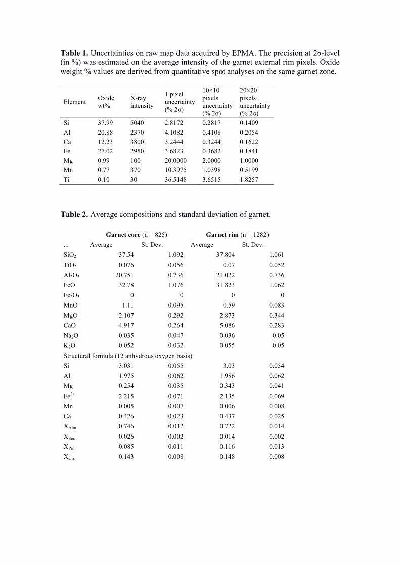
Table 1. Uncertainties on raw map data acquired by EPMA. The precision at 2σ-level (in %) was estimated on the average intensity of the garnet external rim pixels. Oxide weight % values are derived from quantitative spot analyses on the same garnet zone.

Element Oxide wt%

X-ray intensity

1 pixel uncertainty (% 2σ)

10×10 pixels uncertainty (% 2σ)

20×20 pixels uncertainty (% 2σ)

Si 37.99 5040 2.8172 0.2817 0.1409 Al 20.88 2370 4.1082 0.4108 0.2054 Ca 12.23 3800 3.2444 0.3244 0.1622 Fe 27.02 2950 3.6823 0.3682 0.1841 Mg 0.99 100 20.0000 2.0000 1.0000 Mn 0.77 370 10.3975 1.0398 0.5199 Ti 0.10 30 36.5148 3.6515 1.8257

Table 2. Average compositions and standard deviation of garnet.

Garnet core (n = 825) Garnet rim (n = 1282)

... Average St. Dev. Average St. Dev. SiO2 37.54 1.092 37.804 1.061 TiO2 0.076 0.056 0.07 0.052 Al2O3 20.751 0.736 21.022 0.736 FeO 32.78 1.076 31.823 1.062 Fe2O3 0 0 0 0 MnO 1.11 0.095 0.59 0.083 MgO 2.107 0.292 2.873 0.344 CaO 4.917 0.264 5.086 0.283 Na2O 0.035 0.047 0.036 0.05 K2O 0.052 0.032 0.055 0.05 Structural formula (12 anhydrous oxygen basis) Si 3.031 0.055 3.03 0.054 Al 1.975 0.062 1.986 0.062 Mg 0.254 0.035 0.343 0.041 Fe2+ 2.215 0.071 2.135 0.069 Mn 0.005 0.007 0.006 0.008 Ca 0.426 0.023 0.437 0.025 XAlm 0.746 0.012 0.722 0.014 XSps 0.026 0.002 0.014 0.002 XPrp 0.085 0.011 0.116 0.013 XGrs 0.143 0.008 0.148 0.008